Optimization
Chapter 6 of the second volume collects the optimisation methods that machine learning needs beyond textbook gradient descent. Automatic differentiation computes derivatives of programs; stochastic optimisation estimates gradients of expectations, with the score-function and reparameterisation estimators for distributions that depend on the parameters; natural gradient descent measures steps by the Kullback–Leibler divergence they induce; bound optimisation (MM and EM) climbs a sequence of surrogates; Bayesian optimisation and derivative-free search handle expensive or non-differentiable objectives; optimal transport and submodular optimisation treat distributions and subsets as the objects being optimised. The supplement adds proximal methods, dynamic programming, conjugate duality and the Bayesian learning rule, which unifies several optimisers as natural-gradient steps on a variational objective. The notes prove what the book states without proof, correct a handful of slips, and check the claims on small computed examples.
Ch. 1 Introduction Ch. 2 Probability Ch. 3 Statistics Ch. 4 Graphical models Ch. 5 Information theory Ch. 6 Optimisation Ch. 7 Inference algorithms Ch. 8 Gaussian filtering Ch. 9 Message passing Ch. 10 Variational inference Ch. 11 Monte Carlo Ch. 12 MCMC Ch. 13 Sequential Monte Carlo Ch. 14 Predictive models Ch. 15 GLMs Ch. 16 Deep networks Ch. 17 Bayesian neural networks Ch. 18 Gaussian processes Ch. 19 Beyond iid Ch. 20 Generative models Ch. 21 VAEs Ch. 22 Autoregressive models Ch. 23 Normalizing flows Ch. 24 Energy-based models Ch. 25 Diffusion models Ch. 26 GANs Ch. 27 Discovery methods Ch. 28 Latent factor models Ch. 29 State-space models Ch. 30 Graph learning Ch. 31 Nonparametric Bayes Ch. 32 Representation learning Ch. 33 Interpretability Ch. 34 Decision making Ch. 35 Reinforcement learning Ch. 36 Causality
How to read these notes
They follow the book. Sections carry the book's numbers (6.4.5, 6.8.3, ...) and equations the book numbers keep their numbers, e.g. \((6.99)\). The four sections of the online supplement (Supplement Chapter 7) are inserted where the main text needs them and labelled (supplement); their equations keep the supplement's numbers (7.x). The chapter has no end-of-chapter exercises, so three short practice problems with solutions close the notes.
Filling the gaps. Wherever the book writes "one can show", quotes a theorem from the literature or sketches a step, an orange Filling the gap box gives the full argument. Proofs start hidden: open one with its bar, or use the buttons below.
Figures and demonstrations. Every computed figure is reproduced by the Python code; the figures that are hand-drawn diagrams (6.1, 6.4, 6.13–6.16 and the supplement's flat-minimum sketch) are not. Supplement Figures 7.2 and 7.3 (a ResNet on CIFAR-10 and surveillance video) are replaced by small computed stand-ins, and the point sets and data of the other figures are simulated or taken from scikit-learn; every caption says so. The ▶ Demo boxes open an interactive demonstration set to the case being discussed.
Main reference
K. P. Murphy, Probabilistic Machine Learning: Advanced Topics, MIT Press (2023; December 2025 draft), Chapter 6, pages 261–344, and the online supplement, Chapter 7 (book page: probml.github.io/pml-book/book2.html). Section, equation and figure numbers refer to this book. The explanations, derivations, figures and code are my own.
Companion courses
- Probabilistic Machine Learning: An Introduction: Chapter 8 (optimisation) proves the convexity facts, gradient descent, SGD (8.4), the \(\ell_1\) proximal operator (8.6) and the general bound-optimisation and EM results (8.7); Section 6.2.4 proves \(\KL\ge0\); gap 10.10 proves the Böhning bound; Section 17.2 is Gaussian processes.
- Bayesian and Probabilistic Machine Learning (Bishop): 9.4 the EM algorithm in general and 10.1 variational inference.
- Foundations of Deep Learning: Chapter 7 (gradient descent) and 8.2 automatic differentiation.
What this chapter adds: the JVP/VJP view of differentiation, gradient estimators for expectations and their variance, the Fisher geometry behind the natural gradient, MM and EM as monotone surrogate methods with new examples, Gaussian-process Bayesian optimisation, population-based search, Kantorovich duality and Sinkhorn, submodularity and the greedy guarantee, and in the supplement proximal methods, conjugate bounds and the Bayesian learning rule.
6.1 Introduction
p. 261 Every method in this chapter solves a problem of the form \(\bm\theta^\ast\in\argmin_{\bm\theta\in\Theta}L(\bm\theta)\) (6.1), but each relaxes a different assumption of the textbook picture of a smooth, convex, deterministic loss that is cheap to differentiate. Automatic differentiation (6.2) removes hand-derived gradients; stochastic optimisation (6.3) lets the loss be an expectation, even over a distribution that depends on \(\bm\theta\); natural gradient descent (6.4) changes the geometry in which steps are measured; bound optimisation (6.5) replaces the loss by simpler surrogates; Bayesian optimisation (6.6) and derivative-free search (6.7) handle objectives without gradients or with expensive evaluations; optimal transport (6.8) is an optimisation problem that compares distributions; submodular optimisation (6.9) handles set functions. The four supplement sections are placed where the main text uses them.
See also: Chapter 8 of the introductory course proves the facts about convexity, gradient descent, Newton and quasi-Newton methods, SGD, Adam and KKT conditions that this chapter takes for granted.
6.2 Automatic differentiation
p. 261 This section (written by R. Frostig) treats differentiation as an operation on functions: the derivative of \(f:\R^n\to\R^m\) is the function \(\partial f\) sending a point \(\bm x\) to the Jacobian, a linear map \(\R^n\to\R^m\), and an automatic differentiation (AD) system only ever has to compute Jacobian-vector and vector-Jacobian products.
6.2.1 Differentiation in functional form
pp. 261–265 Write \(\partial f(\bm x)[\bm v]\) for the Jacobian at the linearisation point \(\bm x\) applied to a perturbation \(\bm v\). The map \((\bm x,\bm v)\mapsto\partial f(\bm x)[\bm v]\) is the Jacobian-vector product (JVP) (6.7), and \((\bm x,\bm u)\mapsto\partial f(\bm x)^\T[\bm u]\) the vector-Jacobian product (VJP) (6.8). Higher derivatives are repeated application, \(\partial^2=\partial\circ\partial\), so the Taylor series reads \[ f(\bm x+\bm v)\approx f(\bm x)+\partial f(\bm x)[\bm v]+\tfrac1{2!}\partial^2f(\bm x)[\bm v,\bm v]+\cdots+\tfrac1{k!}\partial^kf(\bm x)[\bm v,\dots,\bm v]. \tag{6.12} \] For several arguments, \(\partial g(\bm x,\bm y)[\dot{\bm x},\dot{\bm y}]=\partial_1g(\bm x,\bm y)[\dot{\bm x}]+\partial_2g(\bm x,\bm y)[\dot{\bm y}]\) (6.17), and the chain rule \(\partial(g\circ h)(\bm x)=\partial g(h(\bm x))\circ\partial h(\bm x)\) (6.21) handles fan-out: if \(f(\bm x)=g(a(\bm x),b(\bm x))\) then \[ \partial f(\bm x)=\partial_1g(a(\bm x),b(\bm x))\circ\partial a(\bm x)+\partial_2g(a(\bm x),b(\bm x))\circ\partial b(\bm x), \tag{6.24} \] a sum over the paths by which \(\bm x\) reaches the output.
6.2.2 Differentiating chains, circuits, and programs
pp. 266–271 Chains. For \(f=f_T\circ\cdots\circ f_1\), \(\partial f(\bm x)=J_T\cdots J_1\) with \(J_t=\partial f_t(\bm x_{t-1})\), \(\bm x_t=f_t(\bm x_{t-1})\) (6.29). Multiplying from the right gives the JVP in the order of computation: forward mode (Algorithm 6.1), which carries \((\bm x_t,\bm v_t)\) and stores nothing. Transposing gives \(J_1^\T[\cdots J_T^\T[\bm u]]\), which runs backwards and needs the saved points \(\bm x_0,\dots,\bm x_{T-1}\): reverse mode (Algorithm 6.2), the backpropagation algorithm. It is cheaper when the output is a scalar loss and costs memory proportional to the chain length.
Circuits and programs. When primitives take several arguments the computation is a directed acyclic graph (Figure 6.1) with fan-in and fan-out. Forward mode (Algorithm 6.3) sums the partial JVPs over the parents of a node; reverse mode (Algorithm 6.4) goes in reverse topological order and sums the cotangents on the outgoing edges of each node, \(\bm u'_t=\sum_{c\in\mathrm{Ch}(t)}\bm u_{t\to c}\). Loops, branches and recursion are handled by treating a pure functional program as the circuit description, as JAX does.
Filling the gap 6.1: the adjoint identity, the cost of a Jacobian, the fan-out sum, and why a gradient costs a constant multiple of the function pp. 266–270, (6.29)–(6.40), Algorithms 6.1–6.4
Derivation
Adjoint identity. By definition of the transpose of a linear map, \(\langle\bm u,\partial f(\bm x)[\bm v]\rangle=\langle\partial f(\bm x)^\T[\bm u],\bm v\rangle\). Taking \(\bm v=\bm e_i\) gives the \(i\)-th column of the Jacobian \(J\), taking \(\bm u=\bm e_j\) its \(j\)-th row. So the full Jacobian costs \(n\) JVPs or \(m\) VJPs; for a scalar loss (\(m=1\)) the whole gradient is \(\partial f(\bm x)^\T[1]\), one reverse pass whatever \(n\) is. Forward mode wins when \(n<m\).
Chains. Associativity of the matrix product shows that the two bracketings (6.30) and (6.33) give the same answer and differ only in the order of evaluation. Forward mode needs \((\bm x_{t-1},\bm v_{t-1})\) only to produce \((\bm x_t,\bm v_t)\), so its extra memory is a constant multiple of one layer. Reverse mode needs \(J_t^\T\), hence \(\bm x_{t-1}\), in the order \(t=T,\dots,1\), the reverse of the order of creation, so all of \(\bm x_0,\dots,\bm x_{T-1}\) must be stored or recomputed.
Fan-out. Let \(f=f_{bc}\circ\mathrm{dup}\circ a\) with \(\mathrm{dup}(\bm x)=(\bm x,\bm x)\), as in (6.37). Then \(\partial\mathrm{dup}=\binom{I}{I}\) and its transpose \((I\ \ I)\) maps a pair of cotangents \((\bm u_1,\bm u_2)\) to \(\bm u_1+\bm u_2\). Hence \(\partial f(\bm x)^\T=\partial a(\bm x)^\T\circ(I\ \ I)\circ\partial f_{bc}(\cdot)^\T\): the cotangents returning along the two outgoing edges of \(a\) are added. In a general circuit, induct along the reverse topological order: if each child \(c\) of node \(t\) has received the correct cotangent \(\bm u_{t\to c}\) (the transposed derivative of the sink with respect to the input of \(c\) that comes from \(t\)), then by the multivariable chain rule (6.24) the derivative of the sink with respect to \(\bm x_t\) is the sum of the contributions through the children, which is Algorithm 6.4, line 10.
Cost. Suppose evaluating primitive \(f_t\) costs \(c_t\) and its VJP at most \(\kappa c_t\). The forward sweep costs \(\sum_tc_t\), the backward sweep at most \(\kappa\sum_tc_t\), and summing cotangents at fan-out nodes adds a bounded multiple of the same. So a gradient costs a constant multiple of the function, independent of \(n\). The constant is small: for an elementwise map \(\partial f_t^\T\bm u=f_t'(\bm x)\odot\bm u\), so \(\kappa=1\); for \(Y=AB\) with \(A\in\R^{p\times q}\), \(B\in\R^{q\times r}\) (cost \(pqr\)), \(\langle\bar Y,\mathrm dA\,B+A\,\mathrm dB\rangle=\langle\bar YB^\T,\mathrm dA\rangle+\langle A^\T\bar Y,\mathrm dB\rangle\), so the VJP is the pair \((\bar YB^\T,A^\T\bar Y)\), two products of cost \(pqr\): \(\kappa=2\).
Numerical confirmation. For the circuit of Figure 6.1(a) with \(a=\sin\), \(b=\exp\), \(c\) the product, summed to a scalar, the reverse-mode gradient agrees with central finite differences and with PyTorch's autograd to \(10^{-12}\); the Jacobian from \(n\) JVPs equals the one from \(m\) VJPs; and the adjoint identity holds to rounding (circuit_jvp, circuit_vjp in the companion code).
See also: forward-mode and reverse-mode automatic differentiation (Foundations of Deep Learning, Section 8.2).
6.3 Stochastic optimization
p. 271 The objective is now an expectation, \(L(\bm\theta)=\E_{q_{\bm\theta}(\bm z)}[\tilde L(\bm\theta,\bm z)]\) (6.41), where \(\bm z\) is noise, a latent variable or an action.
6.3.1 Stochastic gradient descent
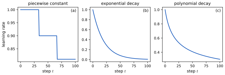
pp. 271–273 If \(\bm g_t\) is an unbiased estimate of \(\nabla L(\bm\theta_t)\) (6.42), SGD is \(\bm\theta_{t+1}=\bm\theta_t-\eta_t\bm g_t\) (6.43). The step size follows a schedule: piecewise constant \(\eta_i\) (6.45), exponential decay \(\eta_0e^{-\lambda t}\) (6.46), or polynomial decay \(\eta_0(\beta t+1)^{-\alpha}\) (6.47), commonly \(\alpha=\tfrac12\). Variance reduction (6.3.1.2) and preconditioning \(\bm\theta_{t+1}=\bm\theta_t-\eta_tC_t\bm g_t\) (6.48, 6.3.1.3) are proved in 8.4.5 and 8.4.6 of the first volume.
Filling the gap 6.2: what the step-size conditions buy: the SGD recursion, a constant-step floor, Robbins–Monro and the \(1/t\) rate pp. 271–272, (6.42)–(6.47)
Derivation
Setting. Let \(L\) be \(\mu\)-strongly convex with \(\ell\)-Lipschitz gradient, minimiser \(\bm\theta^\ast\), and \(\E[\bm g_t\mid\bm\theta_t]=\nabla L(\bm\theta_t)\), \(\E[\|\bm g_t-\nabla L(\bm\theta_t)\|^2\mid\bm\theta_t]\le\sigma^2\). Write \(a_t=\E\|\bm\theta_t-\bm\theta^\ast\|^2\). Strong convexity gives \(\langle\nabla L(\bm\theta),\bm\theta-\bm\theta^\ast\rangle\ge\mu\|\bm\theta-\bm\theta^\ast\|^2\), and since \(\nabla L(\bm\theta^\ast)=0\), \(\|\nabla L(\bm\theta)\|\le\ell\|\bm\theta-\bm\theta^\ast\|\).
The recursion. Expanding the square and conditioning, \(\E\|\bm\theta_{t+1}-\bm\theta^\ast\|^2=\|\bm e_t\|^2-2\eta_t\langle\nabla L,\bm e_t\rangle+\eta_t^2(\|\nabla L\|^2+\E\|\text{noise}\|^2)\le(1-2\eta_t\mu+\eta_t^2\ell^2)\|\bm e_t\|^2+\eta_t^2\sigma^2\), with \(\bm e_t=\bm\theta_t-\bm\theta^\ast\). For \(\eta_t\le\mu/\ell^2\) this gives \[ a_{t+1}\le(1-\mu\eta_t)\,a_t+\eta_t^2\sigma^2. \tag{$\ast$} \]
(a) Constant step. Unrolling \((\ast)\) with \(\eta_t=\eta\): \(a_t\le(1-\mu\eta)^ta_0+\eta^2\sigma^2\sum_{k<t}(1-\mu\eta)^k\le(1-\mu\eta)^ta_0+\eta\sigma^2/\mu\). The first term decays geometrically but the iterates keep fluctuating in a ball of squared radius \(\eta\sigma^2/\mu\): a constant step never converges under gradient noise. (For \(L=\mu\theta^2/2\) and Gaussian noise the exact stationary value is \(\eta\sigma^2/(\mu(2-\eta\mu))\), confirmed by simulation.)
(b) Decreasing step. Suppose \(\eta_t\to0\) and \(\sum\eta_t=\infty\). Given \(\varepsilon>0\) pick \(T\) with \(\eta_t\sigma^2\le\mu\varepsilon/2\) for \(t\ge T\). Then \(\eta_t^2\sigma^2\le\mu\eta_t\varepsilon/2\) and \((\ast)\) gives \(a_{t+1}-\varepsilon/2\le(1-\mu\eta_t)(a_t-\varepsilon/2)\), so \((a_t-\varepsilon/2)_+\le\prod_{s=T}^{t-1}(1-\mu\eta_s)(a_T-\varepsilon/2)_+\le e^{-\mu\sum_{s=T}^{t-1}\eta_s}(a_T)\to0\). Hence \(\limsup a_t\le\varepsilon/2\) for every \(\varepsilon\), i.e. \(a_t\to0\). The conditions \(\sum\eta_t=\infty\) (reach the optimum from anywhere) and \(\eta_t\to0\) (damp the noise) are the Robbins–Monro conditions; for merely convex losses one also needs \(\sum\eta_t^2<\infty\). The printed (6.44), "\(\sum\eta_t^2/\sum\eta_t\to0\)", is a garbled form of these (see the notes on the book).
(c) The \(1/t\) rate. Take \(\eta_t=2/(\mu(t+t_0))\) with \(t_0\ge2\ell^2/\mu^2\) (so \(\eta_t\le\mu/\ell^2\)) and \(C=\max(t_0a_0,\,4\sigma^2/\mu^2)\). Claim \(a_t\le C/(t+t_0)\). True at \(t=0\). If true at \(t\), with \(s=t+t_0\), \((\ast)\) gives \(a_{t+1}\le(1-2/s)C/s+4\sigma^2/(\mu^2s^2)\le C/s-2C/s^2+C/s^2=C/s-C/s^2\le C/(s+1)\), because \(\tfrac1s-\tfrac1{s+1}=\tfrac1{s(s+1)}\le\tfrac1{s^2}\). So SGD with this schedule has \(\E\|\bm\theta_t-\bm\theta^\ast\|^2=O(1/t)\).
6.3.2 SGD for optimizing a finite-sum objective
p. 273 If \(q\) does not depend on \(\bm\theta\), the gradient passes inside the expectation, \(\nabla L=\E[\nabla\tilde L]\approx\frac1S\sum_s\nabla\tilde L(\bm\theta,\bm z_s)\) (6.49). With the empirical distribution this is empirical risk minimisation (6.50) and a minibatch of \(B\) examples gives (6.52); the unbiasedness and variance are proved in gap 8.8 of the first volume.
6.3.3 SGD for optimizing the parameters of a distribution
pp. 273–274 When \(q_{\bm\theta}\) depends on \(\bm\theta\), the product rule splits the gradient into \(\int\nabla_\theta\tilde L\,q\,\mathrm d\bm z\) (Monte Carlo as before) and the problematic \(I=\int\tilde L\,\nabla_\theta q\,\mathrm d\bm z\) (6.56). Two estimators approximate \(I\).
6.3.4 Score function estimator (REINFORCE)
pp. 274–275 The log-derivative trick \(\nabla q=q\nabla\log q\) (6.57) turns (6.56) into \(I=\E_q[\tilde L\nabla_\theta\log q]\) (6.58), estimated by (6.59). It needs only that one can sample from and differentiate \(q\); \(\tilde L\) may be a black box. The variance is reduced by a control variate (6.60) or by Rao–Blackwellisation (6.61).
Filling the gap 6.3: the score-function estimator is unbiased, its variance, control variates and Rao–Blackwellisation pp. 274–275, (6.57)–(6.61)
Derivation
Unbiasedness. Assume \(|\partial_\theta(\tilde L q_\theta)|\) is dominated by an integrable function so that differentiation and integration commute (dominated convergence). Then \(\nabla\int\tilde Lq_\theta=\int\tilde L\nabla q_\theta=\int\tilde L\,q_\theta\nabla\log q_\theta=\E[\tilde L\nabla\log q_\theta]\). Taking \(\tilde L\equiv1\) shows that the score has mean zero: \(\E[\nabla\log q_\theta]=\nabla\int q_\theta=\nabla1=0\).
Why the variance is large. For a constant \(\tilde L\equiv c\) the true gradient is 0 yet each sample gives \(c\nabla\log q_\theta(\bm z)\) with covariance \(c^2F(\bm\theta)\) (the Fisher matrix): the estimator is as noisy as the magnitude of \(\tilde L\), not of its variation. Subtracting a constant baseline \(b\) leaves the mean unchanged, since \(\E[b\nabla\log q]=0\), and the optimal scalar-parameter baseline is \(b^\ast=\E[\tilde Ls^2]/\E[s^2]\) with \(s=\partial_\theta\log q\).
Control variates. Let \(Y\) be an unbiased estimate and \(B\) a variable with known mean. For \(\hat Y=Y-c(B-\E B)\): \(\E\hat Y=\E Y\) and \(\var\hat Y=\var Y-2c\cov(Y,B)+c^2\var B\), minimised at \(c^\ast=\cov(Y,B)/\var B\) with value \((1-\rho^2)\var Y\), \(\rho=\operatorname{corr}(Y,B)\). Never worse than \(c=0\); a correlated \(B\) always helps (the book's (6.60) is this with \(B\) a baseline function of \(\bm z\)). In the example of Section 6.3.5.1 below with \(B=(z-\mu)^2\) (mean \(v\)) the optimal \(c^\ast\) reduces the variance, as checked numerically.
Rao–Blackwellisation. For discrete \(\bm z\), split the support into a small set \(S_1\) and the rest \(S_2\): \(\nabla L=\sum_{S_1}\tilde L\nabla q+\sum_{S_2}\tilde L\,q\nabla\log q=\sum_{S_1}\tilde L\nabla q+q(S_2)\,\E[\tilde L\nabla\log q\mid\bm z\in S_2]\). The weight \(q_\theta(S_2)=\Pr(\bm z\in S_2)\) multiplies the conditional expectation, and it is missing from the printed (6.61). Estimating only the second term by sampling gives an estimator that is conditionally unbiased given the enumerated part; by the law of total variance, \(\var(Y)=\E\var(Y\mid\mathcal G)+\var\E(Y\mid\mathcal G)\ge\var\E(Y\mid\mathcal G)\), replacing a quantity by its conditional expectation never increases variance.
6.3.5 Reparameterization trick
pp. 275–277 If \(\bm z=g(\bm\theta,\bm\epsilon)\) with \(\bm\epsilon\sim q_0\) independent of \(\bm\theta\) (for example \(z=\mu+\sigma\epsilon\), (6.62)), then \(L=\E_{q_0}[\tilde L(\bm\theta,g(\bm\theta,\bm\epsilon))]\) and the gradient moves inside, \(\nabla L=\E_{q_0}[\nabla_\theta\tilde L(\bm\theta,g(\bm\theta,\bm\epsilon))]\) (6.64), the pathwise derivative. It requires \(\tilde L\) to be differentiable in \(\bm z\) but typically has much lower variance than the score function. The gradient inside is the total derivative \(\nabla_{\bm z}\tilde L\,J+\nabla_\theta\tilde L\) with \(J=\partial\bm z/\partial\bm\theta\) (6.68–6.70).
Example 6.3.5.1. For \(\tilde L(z)=z^2-3z\) and \(z\sim\N(\mu,v)\), \(L(\mu,v)=\mu^2+v-3\mu\), so the exact gradient is \((2\mu-3,\,1)\). Bonnet's and Price's theorems (6.66)–(6.67) give the same numbers without sampling: \(\E[\tilde L'(z)]=2\mu-3\) and \(\tfrac12\E[\tilde L''(z)]=1\).
Filling the gap 6.4: Bonnet's and Price's theorems, and the variance of the two estimators in the example pp. 276, 285, (6.66)–(6.67), (6.106)–(6.107)
Derivation
Bonnet (Stein's lemma). Let \(f\) be absolutely continuous with \(f,f'\) of polynomial growth and \(z\sim\N(\mu,v)\), density \(N(z)\). Since \(\partial_\mu N=-\partial_zN\), \(\partial_\mu\E f(z)=\int f\,\partial_\mu N\,\mathrm dz=-\int f\,\partial_zN\,\mathrm dz=\int f'N\,\mathrm dz=\E f'(z)\), integrating by parts (the boundary term vanishes because \(N\) decays faster than \(f\) grows). Equivalent form: \(\E[(z-\mu)f(z)]=v\,\E f'(z)\).
Price. The Gaussian density solves the heat equation \(\partial_vN=\tfrac12\partial_z^2N\): with \(N=(2\pi v)^{-1/2}e^{-(z-\mu)^2/2v}\), \(\partial_vN=N\big(-\tfrac1{2v}+\tfrac{(z-\mu)^2}{2v^2}\big)\) and \(\partial_z^2N=N\big(\tfrac{(z-\mu)^2}{v^2}-\tfrac1v\big)\). Hence \(\partial_v\E f=\tfrac12\int f\,\partial_z^2N=\tfrac12\E f''(z)\) after two integrations by parts. In several dimensions \(\nabla_V\E f=\tfrac12\E\nabla^2f\) when the entries of the symmetric matrix \(V\) are treated as independent (the factor \(c_{ij}\) in (6.107) only reflects how the off-diagonal entries are counted). Check: for \(f=\sin\), \(\E\sin z=e^{-v/2}\sin\mu\), so \(\partial_\mu=e^{-v/2}\cos\mu=\E\cos z\) and \(\partial_v=-\tfrac12e^{-v/2}\sin\mu=\tfrac12\E(-\sin z)\), as the theorems say.
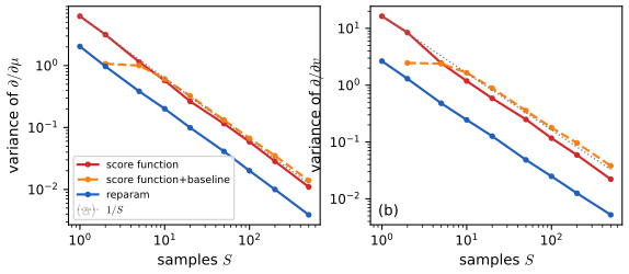
Variances in the example. The reparameterisation estimator of \(\partial_\mu\) from one sample is \(2z-3\), of variance \(4v\). For the score function, \(z=\mu+\sqrt v\epsilon\) and \(g=\tilde L(z)(z-\mu)/v=\frac{\mu^2-3\mu}{\sqrt v}\epsilon+(2\mu-3)\epsilon^2+\sqrt v\epsilon^3\); using \(\var\epsilon^2=2\), \(\var\epsilon^3=15\), \(\cov(\epsilon,\epsilon^3)=3\), \[ \var g=\frac{(\mu^2-3\mu)^2}{v}+2(2\mu-3)^2+15v+6(\mu^2-3\mu). \] At \(\mu=1\), \(v=\tfrac12\) this is \(5.5\) against \(2\) for the pathwise estimator; both are unbiased, and simulation agrees (Figure x6.c: the variance falls like \(1/S\) for both, with the pathwise curve lower).
6.3.5.3 "Sticking the landing" estimator
p. 277 For the ELBO \(\tilde L=\log p(\bm z,\bm x)-\log q(\bm z\given\bm\theta)\) (6.71) the gradient splits into a path derivative and a score term, \(\nabla_{\bm z}[\log p-\log q]J-\nabla_\theta\log q(\bm z\given\bm\theta)\) (6.73). The score term has mean zero but is not zero for finite \(S\); the STL estimator drops it by differentiating \(\log q(\bm z\given\bm\theta')\) at a stop-gradient copy \(\bm\theta'\) (6.74–6.77).
Filling the gap 6.5: why dropping the score term is unbiased, and why the estimator has zero variance at the optimum p. 277, (6.71)–(6.77)
Derivation
Unbiased. The dropped term is \(\E_{q_0}[\nabla_\theta\log q(\bm z\given\bm\theta')\mid_{\bm\theta'=\bm\theta}]\) with \(\bm z\sim q_\theta\), the expected score, which is 0 (Gap 6.3). Thus STL has the same mean as the standard pathwise estimator.
Zero variance at the optimum. If \(q(\cdot\given\bm\theta)=p(\cdot\given\bm x)\) then \(\log p(\bm z,\bm x)-\log q(\bm z)=\log p(\bm x)\) is constant in \(\bm z\), so its \(\bm z\)-gradient is exactly 0 for every sample: the STL estimator returns 0 with no Monte Carlo noise. The standard estimator still adds the sampled score \(\nabla_\theta\log q(\bm z)\), nonzero for each draw. Check: with \(p(z)=\N(0,1)\), \(p(x\given z)=\N(z,1)\), \(x=0.7\), the posterior is \(\N(x/2,1/2)\) and \(\partial_z[\log p(z,x)-\log q(z)]=-z+(x-z)+(z-\mu_q)/s_q^2\) vanishes identically at \(q=\)posterior. (STL is not always better away from the optimum; a weighted combination can be optimised, as the book notes.)
6.3.6 Gumbel softmax trick
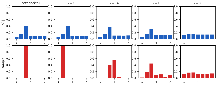
pp. 277–278 A one-hot categorical sample \(\bm d\sim\mathrm{Cat}(\bm\alpha)\) is not reparameterisable, but \(\bm d=\mathrm{onehot}(\argmax_k[\epsilon_k+\log\alpha_k])\) with \(\epsilon_k\sim\mathrm{Gumbel}(0,1)\), \(\epsilon_k=-\log(-\log u_k)\) (the Gumbel-max trick, (6.78)), moves the randomness into parameter-free noise. Replacing the argmax by a softmax with temperature \(\tau\), \(x_k=\exp((\log\alpha_k+\epsilon_k)/\tau)/\sum_{k'}\exp((\log\alpha_{k'}+\epsilon_{k'})/\tau)\) (6.79), gives a differentiable relaxation on the simplex, the concrete distribution.
Filling the gap 6.6: the Gumbel-max trick and the two limits of the Gumbel softmax pp. 277–278, (6.78)–(6.79)
Derivation
Gumbel-max. Let \(\epsilon_k\) be i.i.d. standard Gumbel with cdf \(F(t)=e^{-e^{-t}}\) and put \(a_k=\log\alpha_k\). Then \(\Pr(\argmax_k(a_k+\epsilon_k)=j)=\int f(t-a_j)\prod_{k\ne j}F(t-a_k)\,\mathrm dt\) with \(f=F'\), \(f(t)=e^{-t}e^{-e^{-t}}\). Now \(\prod_{k\ne j}F(t-a_k)=\exp(-e^{-t}\sum_{k\ne j}\alpha_k)\) and \(f(t-a_j)=\alpha_je^{-t}\exp(-\alpha_je^{-t})\), so the integrand is \(\alpha_je^{-t}\exp(-A e^{-t})\) with \(A=\sum_k\alpha_k\). With \(w=e^{-t}\), \(\int_0^\infty\alpha_je^{-Aw}\mathrm dw=\alpha_j/A=\pi_j\). That is exactly \(\mathrm{Cat}(\bm\pi)\) with \(\pi_j=\alpha_j/\sum\alpha_k\). The inverse-cdf recipe \(\epsilon=-\log(-\log u)\), \(u\sim U(0,1)\), is correct since \(\Pr(\epsilon\le t)=\Pr(u\le e^{-e^{-t}})=F(t)\).
Limits. The softmax of \(\bm s/\tau\) tends, as \(\tau\to0\), to the one-hot vector of \(\argmax_k s_k\) whenever the maximum is unique (an event of probability one), because \(\exp((s_k-s_j)/\tau)\to0\) for \(s_k<s_j\); so the relaxed sample converges almost surely to the Gumbel-max sample. As \(\tau\to\infty\), \(\exp(s_k/\tau)\to1\) and \(x_k\to1/K\). The relaxation is differentiable in \(\log\alpha\) for \(\tau>0\), at the price of a bias (the relaxed variable is not one-hot) that grows with \(\tau\), while small \(\tau\) gives large-variance gradients.
6.3.7 Stochastic computation graphs
p. 278 Functions with both deterministic and stochastic nodes can be differentiated by combining Section 6.2 with the score-function and reparameterisation estimators: each stochastic node contributes a score term or a pathwise term (Schulman et al., 2015).
6.3.8 Straight-through estimator
p. 279 For a hard threshold \(f(x)=\ind(x>0)\) the derivative is 0 almost everywhere; the straight-through estimator (Bengio et al., 2013) backpropagates the identity (or hard tanh (6.81)) in its place.
Filling the gap 6.7: what the straight-through estimator estimates p. 279, (6.80)–(6.81)
Derivation
Make the unit stochastic: \(b=\ind(a+\epsilon>0)\) with \(\epsilon\) logistic, so \(\Pr(b=1)=\sigma(a)\). For any downstream loss \(h(b)\), \(\E h(b)=\sigma(a)h(1)+(1-\sigma(a))h(0)\) and the exact derivative is \(\frac{\mathrm d}{\mathrm da}\E h(b)=\sigma(a)(1-\sigma(a))\,[h(1)-h(0)]\). The straight-through rule backpropagates \(h'(b)\) times the identity, giving \(\E[h'(b)]\). For \(h\) linear, \(h'=h(1)-h(0)\) and ST returns that slope while the truth is \(\sigma'(a)\le\tfrac14\) times it: same sign, wrong scale. So ST is a biased but positively correlated surrogate; it is exact only where the derivative of \(\E[b]\) is 1 (a linear gate). The hard-tanh clipping keeps the backpropagated gradients from growing.
6.4 Natural gradient descent
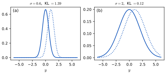
pp. 279–286 Natural gradient descent (NGD; Amari, 1998) optimises the parameters of a distribution \(p_{\bm\theta}(y\given\bm x)\) by measuring distances between the induced distributions rather than between parameter vectors. Figure 6.5: shifting a Gaussian mean by \(\delta\) changes the distribution far more when the variance is small, which the Euclidean distance \((\mu-\mu')^2+(\sigma-\sigma')^2\) ignores.
6.4.1 Defining the natural gradient
pp. 280–281 For one input, \(\KL(p_{\bm\theta}(y\given\bm x)\,\|\,p_{\bm\theta+\bm\delta}(y\given\bm x))\approx\tfrac12\bm\delta^\T F_x\bm\delta\) (6.82), with Fisher information matrix \(F_x(\bm\theta)=-\E_{p_\theta(y\given x)}[\nabla^2\log p_\theta]=\E[\nabla\log p_\theta\,\nabla\log p_\theta^\T]\) (6.83), averaged over inputs as \(F=\E_{p_D(\bm x)}[F_x]\) (6.84). NGD preconditions by the inverse FIM, \(\bm\theta_{t+1}=\bm\theta_t-\eta_tF(\bm\theta_t)^{-1}\bm g_t\) (6.85); \(\tilde\nabla L=F^{-1}\nabla L\) is the natural gradient (6.86).
Filling the gap 6.8: the two forms of the Fisher matrix, the quadratic approximation of the KL, and why \(F^{-1}g\) is steepest descent for the KL pp. 280–281, (6.82)–(6.86)
Derivation
Two forms of \(F\). Assume \(p_\theta\) is twice differentiable in \(\theta\) with differentiation under the integral allowed. From \(\int p_\theta=1\): \(0=\nabla\int p_\theta=\int p_\theta\nabla\log p_\theta=\E[\nabla\log p_\theta]\); differentiating again, \(0=\int(\nabla^2\log p_\theta+\nabla\log p_\theta\nabla\log p_\theta^\T)p_\theta\), i.e. \(-\E[\nabla^2\log p_\theta]=\E[\nabla\log p_\theta\nabla\log p_\theta^\T]=F\) (6.83).
Quadratic KL. Put \(D(\bm\delta)=\KL(p_\theta\|p_{\theta+\delta})=\E_{p_\theta}[\log p_\theta-\log p_{\theta+\delta}]\). Then \(D(0)=0\), \(\nabla D(0)=-\E[\nabla\log p_\theta]=0\) and \(\nabla^2D(0)=-\E[\nabla^2\log p_\theta]=F\). Taylor's theorem gives \(D(\bm\delta)=\tfrac12\bm\delta^\T F\bm\delta+O(\|\bm\delta\|^3)\) (6.82). (Numerically, for \(\N(\mu,\sigma^2)\) with \(F=\diag(1/\sigma^2,2/\sigma^2)\) in \((\mu,\sigma)\), the ratio of the exact KL to the quadratic form is \(1+O(\|\delta\|)\).)
Steepest descent in KL. Among steps with \(\tfrac12\bm\delta^\T F\bm\delta\le\varepsilon\), minimise the linearised loss change \(\bm g^\T\bm\delta\). With \(\bm a=F^{-1/2}\bm g\) and \(\bm b=F^{1/2}\bm\delta\), \(\bm g^\T\bm\delta=\bm a^\T\bm b\ge-\|\bm a\|\|\bm b\|\ge-\sqrt{2\varepsilon}\sqrt{\bm g^\T F^{-1}\bm g}\), with equality iff \(\bm b=-\sqrt{2\varepsilon}\,\bm a/\|\bm a\|\), i.e. \[ \bm\delta^\ast=-\sqrt{\frac{2\varepsilon}{\bm g^\T F^{-1}\bm g}}\;F^{-1}\bm g. \] So the natural gradient is the direction of steepest descent when length is measured by the KL, as the gradient is for the Euclidean norm.
6.4.2 Interpretations of NGD
p. 281 Trust region. Gradient descent minimises the model \(L+\bm g^\T\bm\delta+\eta\|\bm\delta\|^2\) (6.87); replacing \(\|\bm\delta\|^2\) by \(\|\bm\delta\|_F^2=\bm\delta^\T F\bm\delta\), the squared Euclidean distance in the whitened coordinates \(\bm\phi=F^{1/2}\bm\theta\) (6.88), gives (6.89) and the natural gradient direction (6.90). Gauss–Newton. For an exponential-family likelihood with natural parameter \(\bm\eta=f(\bm x,\bm\theta)\), NGD equals the generalised Gauss–Newton method.
Filling the gap 6.9: invariance to the parameterisation, the trust-region constant, and NGD = generalised Gauss–Newton pp. 281–282, (6.87)–(6.90)
Derivation
Invariance. Let \(\bm\theta=\bm\theta(\bm\phi)\) be a smooth reparameterisation with \(J=\partial\bm\theta/\partial\bm\phi\) invertible. The score transforms as \(\nabla_\phi\log p=J^\T\nabla_\theta\log p\), hence \(F_\phi=J^\T F_\theta J\) and \(\bm g_\phi=J^\T\bm g_\theta\). The natural-gradient step in \(\phi\) is \(\delta\phi=-\eta F_\phi^{-1}\bm g_\phi=-\eta J^{-1}F_\theta^{-1}J^{-\T}J^\T\bm g_\theta=-\eta J^{-1}F_\theta^{-1}\bm g_\theta\), and mapping back, \(\delta\bm\theta\approx J\delta\bm\phi=-\eta F_\theta^{-1}\bm g_\theta\): the same step to first order (the gradient-flow limit is exactly invariant). Steepest descent has no such property, since \(\bm g_\phi=J^\T\bm g_\theta\) maps back to \(JJ^\T\bm g_\theta\ne\bm g_\theta\). The check in the demo: steepest descent fitting a Gaussian in \((\mu,\sigma)\) and in \((\mu,\log\sigma)\) follows different paths while natural gradient follows almost the same one.
Trust-region constant. The model \(M(\bm\delta)=L+\bm g^\T\bm\delta+\eta\bm\delta^\T F\bm\delta\) is minimised at \(\bm\delta=-F^{-1}\bm g/(2\eta)\); the printed (6.90) \(\bm\delta=-\eta F^{-1}\bm g\) is the minimiser of \(L+\bm g^\T\bm\delta+\tfrac1{2\eta}\bm\delta^\T F\bm\delta\). The conclusion (the natural-gradient direction, step set by the penalty weight) is unaffected.
NGD = GGN. Let \(p(y\given\bm x,\bm\theta)=h(y)\exp(\bm\eta^\T T(y)-A(\bm\eta))\) with \(\bm\eta=f(\bm x,\bm\theta)\). The NLL is \(\ell=A(\bm\eta)-\bm\eta^\T T(y)\) and \(\nabla_\theta\ell=J^\T(\nabla A-T)\) with \(J=\partial f/\partial\theta\). Differentiating again, \(\nabla^2_\theta\ell=J^\T\nabla^2A\,J+\sum_k(\partial_kA-T_k)\nabla^2f_k\). The generalised Gauss–Newton matrix keeps the first term, \(G=J^\T\nabla^2A\,J\). Meanwhile \(\E_y[T(y)]=\nabla A(\bm\eta)\), so the expectation of the second term vanishes and \(F=\E_y[\nabla^2\ell]=J^\T\nabla^2A\,J=G\). For logistic regression (\(\bm\eta=\bm\theta^\T\bm x\), linear) \(\nabla^2f=0\), so Newton, Fisher scoring, GGN and NGD coincide. Numerically, for a Bernoulli model with \(\eta=\tanh(\theta_1x)+\theta_2\), the exact Fisher matrix (sum over \(y\in\{0,1\}\)) equals \(J^\T\operatorname{diag}(\sigma(1-\sigma))J\) to rounding.
6.4.3 Benefits of NGD
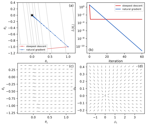
p. 282 \(F\) is positive semidefinite (an expected outer product) while the Hessian can have negative eigenvalues at saddles; \(F\) is easy to estimate from minibatches; and NGD takes large steps where the output barely depends on the parameters. The book's example is the coupled Gaussian \(p(\bm x;\bm\theta)=\N(\bm x\given(3\theta_1+\theta_2/3,\ \theta_1/3),\bm I)\) (6.91) with cross entropy \(L(\bm\theta)=-\E_{p^\ast}[\log p(\bm x;\bm\theta)]\) (6.92). The mean is linear, \(\bm\mu=J\bm\theta\) with \(J=\begin{pmatrix}3&1/3\\1/3&0\end{pmatrix}\); with \(p^\ast=p(\cdot;\bm0)\) we get \(L=\tfrac12\bm\theta^\T F\bm\theta+\const\) and \(F=J^\T J=\begin{pmatrix}3^2+3^{-2}&1\\1&3^{-2}\end{pmatrix}\) (6.94), with eigenvalues 9.21 and 0.0013 (condition number about 6900). Steepest descent with the best fixed step \(1/\lambda_{\max}\) crosses the narrow valley in one step and then crawls; the natural-gradient step \(\bm\theta-\eta F^{-1}F\bm\theta=(1-\eta)\bm\theta\) contracts every direction by the same factor, and with \(\eta=1\) lands on the optimum in one step.
6.4.4 Approximating the natural gradient
pp. 282–284 Forming and inverting \(F\) is costly. Approximations: diagonal (LeCun et al., 1998), low-rank plus block-diagonal, Kronecker-factored blocks (KFAC), truncated conjugate gradients with Hessian-vector products (Hessian-free), and the empirical Fisher \(F\approx\frac1{|D|}\sum_{(x,y)\in D}\nabla\log p(y\given x,\theta)\nabla\log p(y\given x,\theta)^\T\) (6.95–6.97), obtained by replacing the model's \(y\) by the observed one.
Filling the gap 6.10: the empirical Fisher is not the Fisher: when they agree and when it becomes singular pp. 283–284, (6.95)–(6.97)
Derivation
They agree for a correct model, at the data's parameter. If \((\bm x,y)\sim p_D\) and \(p_D(y\given\bm x)=p(y\given\bm x,\bm\theta_0)\) then at \(\bm\theta_0\), \(\E_{p_D}[\nabla\log p\nabla\log p^\T]=\E_{p_D(x)}\E_{p_{\theta_0}(y\mid x)}[\cdots]=F(\bm\theta_0)\). Away from \(\bm\theta_0\), or for a misspecified model, the expectation is over the wrong \(y\) and the two differ.
Example: linear regression. With \(p(y\given\bm x,\bm\theta)=\N(y\given\bm\theta^\T\bm x,1)\) the score is \((y-\bm\theta^\T\bm x)\bm x\), so \(F=\frac1N\sum_n\bm x_n\bm x_n^\T\) (independent of \(\bm\theta\) and of the labels) while the empirical Fisher is \(\frac1N\sum_nr_n^2\bm x_n\bm x_n^\T\) with residuals \(r_n=y_n-\bm\theta^\T\bm x_n\). It is rescaled by the squared residuals and vanishes when the model interpolates, \(r_n=0\), although the true \(F\) is unchanged. A preconditioner \((\mathrm{EF})^{-1}\) then blows up (the plateau problem the book mentions: where the gradient is small the empirical Fisher is nearly singular and the update is unstable), whereas \(F\) marginalises over \(y\) and still sees the sensitivity of the outputs. At a stationary point \(\bar{\bm g}=\frac1N\sum\bm g_n=0\), so the empirical Fisher equals the covariance of the per-example gradients; the sandwich (Godambe) form \(H^{-1}(\mathrm{EF})H^{-1}\), which estimates the covariance of a misspecified maximum-likelihood estimate, is the right use of it. Confirmed numerically: for \(5\) points in \(\R^8\) the least-squares interpolant has \(\|\mathrm{EF}\|\approx10^{-16}\) and \(\|F\|\gg1\).
6.4.5 Natural gradients for the exponential family
pp. 284–286 Take \(L(\bm\mu)=\E_{q_\mu(\bm z)}[\tilde L(\bm z)]\) with \(q\) in an exponential family with moment parameters \(\bm\mu\) (6.98). Then the gradient in the moment parameters equals the natural gradient in the natural parameters \(\bm\lambda\): \(\tilde\nabla_\lambda L=F(\bm\lambda)^{-1}\nabla_\lambda L=\nabla_\mu L\) (6.99–6.101). For \(q=\N(\bm m,V)\) the natural parameters are \((V^{-1}\bm m,-\tfrac12V^{-1})\) and the moment parameters \((\bm m,V+\bm m\bm m^\T)\) (6.102–6.103); (6.108)–(6.111) express \(\nabla_\mu L\) through the gradient and Hessian of \(\tilde L\). For the entropy, \(\tilde\nabla_\lambda H=-\bm\lambda\) when the base measure is constant (6.122).
Filling the gap 6.11: natural gradient in natural parameters = ordinary gradient in moment parameters; the Gaussian formulas; the entropy gradient pp. 284–286, (6.99)–(6.122)
Derivation
(6.99)–(6.101). For \(q_\lambda(z)=h(z)\exp(\bm\lambda^\T T(z)-A(\bm\lambda))\), \(\nabla_\lambda\log q=T-\nabla A\), and \(\bm\mu=\E T=\nabla A(\bm\lambda)\) (Section 3.4.3 of the first volume). Moreover \(F(\bm\lambda)=\E[(T-\bm\mu)(T-\bm\mu)^\T]=\nabla^2A=\partial\bm\mu/\partial\bm\lambda\) (6.100). The chain rule for \(L(\bm\lambda)=L(\bm\mu(\bm\lambda))\) gives \(\nabla_\lambda L=(\partial\bm\mu/\partial\bm\lambda)^\T\nabla_\mu L=F\nabla_\mu L\), hence \(F^{-1}\nabla_\lambda L=\nabla_\mu L\) (6.101). Check, \(L(\bm\mu)=\E z^4=m^4+6m^2v+3v^2\) for the Gaussian: finite differences confirm \(F^{-1}\nabla_\lambda L=\nabla_\mu L\) to \(10^{-4}\).
(6.104)–(6.111). With \(m=\mu^{(1)}\) and \(v=\mu^{(2)}-(\mu^{(1)})^2\): \(\partial v/\partial\mu^{(1)}=-2m\), \(\partial v/\partial\mu^{(2)}=1\), \(\partial m/\partial\mu^{(1)}=1\), \(\partial m/\partial\mu^{(2)}=0\), so \(\partial L/\partial\mu^{(1)}=L_m-2mL_v\) and \(\partial L/\partial\mu^{(2)}=L_v\). By Bonnet and Price (Gap 6.4), \(L_m=\E\tilde L'\) and \(L_v=\tfrac12\E\tilde L''\), giving \(\E\tilde L'-\E\tilde L''\,m\) and \(\tfrac12\E\tilde L''\); in several dimensions (6.108)–(6.111). So natural gradients of Gaussian expectations need the gradient and Hessian of \(\tilde L\). For \(\tilde L=z^4\): \(\E\tilde L'=4(m^3+3mv)\), \(\E\tilde L''=12(m^2+v)\), matching finite differences of \(m^4+6m^2v+3v^2\).
(6.116)–(6.122). With constant \(h\), \(\log q=\bm\lambda^\T T-A\) and \(H(q)=A(\bm\lambda)-\bm\lambda^\T\bm\mu\). Using \(\partial\bm\lambda/\partial\bm\mu=F^{-1}\) (the inverse of (6.100), symmetric): \(\nabla_\mu A(\lambda(\mu))=F^{-1}\nabla_\lambda A=F^{-1}\bm\mu\) and \(\nabla_\mu(\bm\lambda^\T\bm\mu)=\bm\lambda+F^{-1}\bm\mu\). Subtracting, \(\nabla_\mu H=-\bm\lambda\), so \(\tilde\nabla_\lambda H=-\bm\lambda\) (6.122). For the Gaussian, \(H=\tfrac12\log(2\pi e(\mu_2-\mu_1^2))\) gives \(\partial_{\mu_1}H=-m/v=-\lambda_1\) and \(\partial_{\mu_2}H=\tfrac1{2v}=-\lambda_2\).
Stochastic approximation (6.4.5.2). For reparameterisable \(q\), both \(F(\bm\lambda)=\nabla_\lambda\E_q[T]\) and \(\nabla_\lambda\E_q[\tilde L]\) can be written as expectations by pushing the gradient inside (Section 6.3.5), so \(F^{-1}\nabla_\lambda L\) can be estimated by Monte Carlo.
S7.4 The Bayesian learning rule (supplement)
Supp. pp. 76–83 Instead of the point estimate \(\bm\theta^\ast=\argmin\ell(\bm\theta)\), \(\ell(\bm\theta)=\sum_n\ell(y_n,f_\theta(\bm x_n))+R(\bm\theta)\) (7.111), fit a distribution \(q\) by minimising \(\mathcal L(q)=\E_q[\sum_n\ell(y_n,f_\theta(\bm x_n))]+\KL(q\|\pi_0)=\E_q[\ell(\bm\theta)]-H(q)\) (7.112–7.114), with \(\pi_0\propto e^{-R}\). Minimising a perturbation-robust expected loss prefers flat minima away from walls. With \(q\) in an exponential family and natural-gradient descent (Section 6.4) this single rule (the BLR) yields exact Bayes, variational inference, gradient descent, Newton's method, VOGN and RMSprop-type optimisers.
Filling the gap 6.12: BLR: the posterior is the minimiser, the natural-gradient update, and gradient descent, Newton and RMSprop as special cases Supp. pp. 76–82, (7.119)–(7.162)
Derivation
Exact Bayes (7.115)–(7.119). With \(\ell=-\log p(y\given f_\theta(x))\) and \(\pi_0\propto e^{-R}\) the posterior is \(p(\bm\theta\given\mathcal D)=\pi_0\prod_np(y_n\given\cdot)/Z\). Then \(\mathcal L(q)=\E_q[-\log\prod p]+\E_q\log(q/\pi_0)=\E_q\log\frac{q}{\pi_0\prod p}=\KL(q\|p(\cdot\given\mathcal D))-\log Z\), minimised exactly at \(q=p(\cdot\given\mathcal D)\) with value \(-\log Z\). (Verified for Bayesian linear regression: at the Gaussian posterior \(\mathcal L=-\log Z\) and perturbing the mean raises it.)
Update (7.122)–(7.127). For \(q=h\exp(\lambda^\T T-A)\), \(\mathcal L(\lambda)=\E_q\ell-H(q)\), so \(\tilde\nabla_\lambda\mathcal L=\nabla_\mu\E_q\ell-\nabla_\mu H=\nabla_\mu\E_q\ell+\bm\lambda+\nabla_\mu\E_q[\log h]\) (Gap 6.11). NGD gives \(\bm\lambda_{t+1}=\bm\lambda_t-\eta_t\tilde\nabla\mathcal L=(1-\eta_t)\bm\lambda_t-\eta_t\nabla_\mu\E_q[\ell+\log h]\) (7.126), and for constant base measure \(\bm\lambda_{t+1}=(1-\eta_t)\bm\lambda_t-\eta_t\nabla_\mu\E_q\ell\) (7.127). Fixed point: \(\bm\lambda^\ast=\nabla_\mu\E_{q^\ast}[-\ell]\) (7.129); for a conjugate exponential-family model this is \(\bm\lambda_0+\sum_n\tilde{\bm\lambda}_n(y_n)\), the conjugate update (7.130).
Gradient descent (7.133)–(7.137). Take \(q=\N(\bm m,I)\), so \(\bm\lambda=\bm\mu=\bm m\) and \(\log h=-\tfrac12\bm\theta^\T\bm\theta+\const\); then \(\E[\log h]=-\tfrac12(\|\bm m\|^2+D)\), \(\nabla_\mu\E\log h=-\bm m\), and (7.126) gives \(\bm m_{t+1}=(1-\eta)\bm m_t-\eta(\nabla_m\E\ell-\bm m_t)=\bm m_t-\eta\nabla_m\E_q\ell\). By Bonnet, \(\nabla_m\E_q\ell=\E_q\nabla\ell\), and the delta method \(\E_q\nabla\ell\approx\nabla\ell(\bm m)\) gives \(\bm m_{t+1}=\bm m_t-\eta\nabla\ell(\bm m_t)\), gradient descent (exact for quadratic \(\ell\)).
Newton (7.138)–(7.150). Take \(q=\N(\bm m,S^{-1})\) with \(\bm\lambda=(S\bm m,-\tfrac12S)\) and \(\bm\mu=(\bm m,S^{-1}+\bm m\bm m^\T)\). Using (6.109) and (6.111), \(\nabla_{\mu^{(1)}}\E\ell=\E\nabla\ell-\E\nabla^2\ell\,\bm m\) and \(\nabla_{\mu^{(2)}}\E\ell=\tfrac12\E\nabla^2\ell\). The second component of (7.127) is \(-\tfrac12S_{t+1}=-\tfrac12(1-\eta)S_t-\tfrac\eta2\E\nabla^2\ell\), i.e. \(S_{t+1}=(1-\eta)S_t+\eta\E_q\nabla^2\ell\) (7.144); the first is \(S_{t+1}\bm m_{t+1}=(1-\eta)S_t\bm m_t-\eta(\E\nabla\ell-\E\nabla^2\ell\,\bm m_t)=S_{t+1}\bm m_t-\eta\E\nabla\ell\), so \(\bm m_{t+1}=\bm m_t-\eta S_{t+1}^{-1}\E_q\nabla\ell\) (7.147). With \(\eta=1\) and the delta approximation \(\E\nabla^2\ell\approx\nabla^2\ell(\bm m_t)\) this is Newton's method \(\bm m_{t+1}=\bm m_t-[\nabla^2\ell]^{-1}\nabla\ell\) (7.150). Numerically, for a quadratic loss one step with \(\eta=1\) reaches the minimiser and the exact posterior precision; with \(\eta=0.1\), 400 steps converge to the same Gaussian.
VOGN and RMSprop (7.151)–(7.163). A diagonal \(S=\diag(s)\) gives elementwise updates \(\bm\theta_{t+1}=\bm\theta_t-\eta\,\E\nabla\ell/s_{t+1}\), \(s_{t+1}=(1-\eta)s_t+\eta\,\E\,\diag\nabla^2\ell\) (7.151–7.152). Replacing the diagonal Hessian by squared per-example gradients (a Gauss–Newton surrogate, as in Gap 6.9) and the expectations by sampling \(\bm\theta_t+\bm\epsilon\), \(\bm\epsilon\sim\N(0,\diag(s)^{-1})\), gives VOGN (7.156); using the delta method instead gives (7.157)–(7.158), which with separate learning rates and a square root is the RMSprop update (7.162–7.163) (the exponent and constants are heuristic changes the book makes explicit).
Variational optimisation (7.164). For a non-differentiable objective, optimise the parameters of a distribution: \(L(\lambda)=\E_{q_\lambda}[\ell(\bm\theta)]\) is smooth in \(\lambda\) and its gradient is available by the estimators of Section 6.3 (for discrete \(\bm\theta\) with Bernoulli \(q\), \(\lambda_d=\log\frac{p_d}{1-p_d}\), the score-function estimator). Dropping the entropy gives evolution strategies (Section 6.7.6); keeping it lets the variance adapt.
6.5 Bound optimization (MM) algorithms
pp. 287–297 A bound-optimisation or MM (majorise-minimise, minorise-maximise) algorithm builds a surrogate \(Q(\bm\theta,\bm\theta_t)\) that touches the objective at the current point and lies below it everywhere (for maximisation), then maximises the surrogate. Examples: EM, proximal gradient, the mean-shift algorithm.
6.5.1 The general algorithm
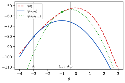
p. 287 If \(Q(\bm\theta,\bm\theta_t)\le\ell(\bm\theta)\) and \(Q(\bm\theta_t,\bm\theta_t)=\ell(\bm\theta_t)\), then \(\bm\theta_{t+1}=\argmax Q(\bm\theta,\bm\theta_t)\) (6.123) increases the objective: \(\ell(\bm\theta_{t+1})\ge Q(\bm\theta_{t+1},\bm\theta_t)\ge Q(\bm\theta_t,\bm\theta_t)=\ell(\bm\theta_t)\) (6.124). Hence a non-monotone log-likelihood is a certain sign of a bug.
6.5.2 Example: logistic regression
pp. 288–289 If a concave \(\ell\) has Hessian \(H(\bm\theta)\succeq B\) for a fixed negative definite \(B\), then \(\ell(\bm\theta)\ge\ell(\bm\theta_t)+(\bm\theta-\bm\theta_t)^\T\bm g_t+\tfrac12(\bm\theta-\bm\theta_t)^\T B(\bm\theta-\bm\theta_t)\) (6.125), and maximising this surrogate gives \(\bm\theta_{t+1}=\bm\theta_t-B^{-1}\bm g_t\) (6.127): a Newton step with a fixed matrix. For softmax regression with \(C-1\) free classes the gradient is \(\sum_n(\bm y_n-\bm p_n)\otimes\bm x_n\) (6.130), the Hessian \(-\sum_n(\diag\bm p_n-\bm p_n\bm p_n^\T)\otimes\bm x_n\bm x_n^\T\) (6.131), and Böhning's bound \(H\succeq-\tfrac12[I-\bm1\bm1^\T/C]\otimes\sum_n\bm x_n\bm x_n^\T\) (6.132); in the binary case \(B=-\tfrac14X^\T X\) (6.133), since \(p_n(1-p_n)\le\tfrac14\).
Filling the gap 6.13: why a Hessian bound gives a minorizer, the contraction rate of the fixed-matrix iteration, and a sign slip in (6.135) pp. 288–289, (6.125)–(6.136)
Derivation
Minorizer. Let \(\bm\delta=\bm\theta-\bm\theta_t\). Taylor's formula with integral remainder: \(\ell(\bm\theta)=\ell(\bm\theta_t)+\bm g_t^\T\bm\delta+\int_0^1(1-s)\,\bm\delta^\T H(\bm\theta_t+s\bm\delta)\bm\delta\,\mathrm ds\). Since \(H\succeq B\) everywhere and \(\int_0^1(1-s)\mathrm ds=\tfrac12\), \(\ell(\bm\theta)\ge\ell(\bm\theta_t)+\bm g_t^\T\bm\delta+\tfrac12\bm\delta^\T B\bm\delta=:Q(\bm\theta,\bm\theta_t)\), with equality at \(\bm\delta=0\): (6.125). The gradient of \(Q\) is \(\bm g_t+B\bm\delta\), zero at \(\bm\delta=-B^{-1}\bm g_t\), the maximiser because \(B\prec0\) (6.127). Monotonicity is (6.124).
Rate. Near the maximiser \(\bm\theta^\ast\), \(\bm e_{t+1}\approx(I-B^{-1}H(\bm\theta^\ast))\bm e_t\). Since \(B\preceq H\preceq0\) we have \(0\preceq-H\preceq-B\), so \((-B)^{-1}(-H)=B^{-1}H\) has eigenvalues in \((0,1]\) and \(I-B^{-1}H\) has eigenvalues in \([0,1)\): the iteration converges linearly, with factor \(1-\lambda_{\min}(B^{-1}H(\bm\theta^\ast))\). The looser the bound (saturated sigmoids, \(p(1-p)\ll\tfrac14\)), the slower; Newton, which uses \(B=H(\bm\theta_t)\), has factor 0 near the optimum (quadratic convergence). The Böhning inequality for \(C>2\) is proved in gap 10.10 of the first volume (and checked numerically here for \(C=3,4,6\)).
Sign. In (6.134) \(B\prec0\), so \(\bm w_{t+1}=\bm w_t-B^{-1}\bm g_t=\bm w_t+4(X^\T X)^{-1}\bm g_t\) when \(\bm g_t=X^\T(\bm y-\bm\mu_t)\) is the gradient of the log-likelihood. The printed (6.135), \(\bm w_t-4(X^\T X)^{-1}\bm g_t\), is the update for the NLL gradient; with the log-likelihood gradient it decreases \(\ell\) (checked numerically on simulated data). Each step costs a solve with the precomputed matrix \(X^\T X\), against \(X^\T S_tX\) rebuilt every step for IRLS (6.136).
6.5.3 The EM algorithm
pp. 289–291 EM computes the MLE or MAP when there are hidden variables \(\bm z_n\) or missing data. Writing \(\ell(\bm\theta)=\sum_n\log\sum_{z_n}p(\bm y_n,\bm z_n\given\bm\theta)\) (6.137) and introducing any distributions \(q_n\), Jensen's inequality gives \(\ell(\bm\theta)\ge\sum_n\{\E_{q_n}[\log p(\bm y_n,\bm z_n\given\bm\theta)]+H(q_n)\}=\mathcal L(\bm\theta,\{q_n\})\) (6.139–6.141), the ELBO. The decomposition \(\mathcal L(\bm\theta,q_n\given\bm y_n)=\log p(\bm y_n\given\bm\theta)-\KL(q_n\|p(\bm z_n\given\bm y_n,\bm\theta))\) (6.145) shows the E step \(q_n^\ast=p(\bm z_n\given\bm y_n,\bm\theta_t)\) makes the bound tight (6.146–6.147); the M step maximises the expected complete-data log-likelihood \(\sum_n\E_{q_n^t}[\log p(\bm y_n,\bm z_n\given\bm\theta)]\) (6.148), which for exponential families depends only on the expected sufficient statistics (6.149) and is solved by moment matching.
Filling the gap 6.14: EM increases the likelihood strictly, its fixed points are stationary points (Fisher's identity), and variational, hard and generalised EM pp. 289–297, (6.137)–(6.150), Section 6.5.6
Derivation
Strict increase. From (6.145) with \(q_n=p(\bm z_n\given\bm y_n,\bm\theta_t)\), for any \(\bm\theta\): \(\ell(\bm\theta)-Q(\bm\theta,\bm\theta_t)=\sum_n\KL(q_n^t\|p(\bm z_n\given\bm y_n,\bm\theta))\ge0\) (KL is nonnegative, Section 6.2.4 of the first volume), with equality at \(\bm\theta=\bm\theta_t\). Hence \(\ell(\bm\theta_{t+1})-\ell(\bm\theta_t)=[Q(\bm\theta_{t+1},\bm\theta_t)-Q(\bm\theta_t,\bm\theta_t)]+\sum_n\KL(q_n^t\|p(\cdot\given\bm y_n,\bm\theta_{t+1}))\), a sum of two nonnegative terms, zero iff \(Q\) did not increase and the posterior did not change. This also proves that any generalised EM step (6.5.6.4), which merely increases \(Q\), increases \(\ell\).
Fisher's identity and stationary points. The function \(\bm\theta\mapsto\ell(\bm\theta)-Q(\bm\theta,\bm\theta_t)\) is differentiable and \(\ge0\) with value 0 at \(\bm\theta_t\), so \(\bm\theta_t\) is its minimiser and its gradient vanishes there: \(\nabla\ell(\bm\theta_t)=\nabla_\theta Q(\bm\theta,\bm\theta_t)\mid_{\bm\theta_t}\). Therefore a fixed point of EM (where the maximiser of \(Q\) is \(\bm\theta_t\) itself, so \(\nabla_\theta Q=0\)) satisfies \(\nabla\ell(\bm\theta_t)=0\): EM stops only at stationary points of the likelihood (saddle points are possible). Numerically on the mixture of Figure 6.7 the two gradients agree to \(10^{-5}\) at \(\bm\theta_t=-3\).
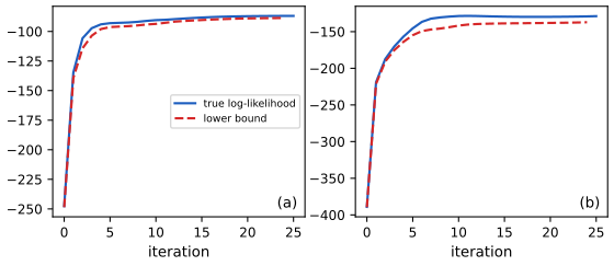
Variational EM (6.5.6.1). With the restricted \(q_n\in\mathcal Q\), the identity (6.145) still holds: \(\mathcal L=\ell-\sum_n\KL(q_n\|p(\cdot\given\bm y_n,\bm\theta))\). Both the E step (maximising \(\mathcal L\) over \(q\)) and the M step (over \(\bm\theta\)) increase \(\mathcal L\), but \(\ell=\mathcal L+\mathrm{KL}\) may fall when the KL term grows (Figure 6.9).
Hard EM (6.5.6.2). Taking \(q_n=\delta_{\hat z_n}\) with \(\hat z_n=\argmax p(z\given\bm y_n,\bm\theta)\) maximises the joint \(\log p(\bm y,\hat{\bm z}\given\bm\theta)\) over \(\bm\theta\) and \(\hat{\bm z}\); there is one latent variable per data point, so the number of nuisance parameters grows with \(N\) and the estimates are in general inconsistent and prone to overfit (for example, a mixture component can collapse on one point). Monte Carlo and stochastic-approximation EM replace the expected statistics by averages over posterior draws; ECM maximises the parameter blocks in turn; online EM updates expected statistics incrementally (incremental EM) or with a step size (stepwise EM).
6.5.4 Example: EM for an MVN with missing data
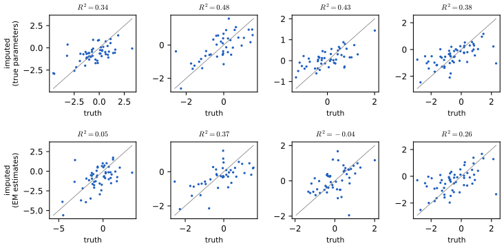
pp. 291–293 Under missing at random, \(\log p(X\given\bm\theta)=\sum_n\log\int p(\bm x_n,\bm z_n\given\bm\theta)\mathrm d\bm z_n\) with \(\bm x_n\) the observed and \(\bm z_n\) the hidden entries (6.151). The E step needs, per row, \(p(\bm z_n\given\bm x_n,\bm\theta)=\N(\bm m_n,V_n)\) with \(\bm m_n=\bm\mu_h+\Sigma_{hv}\Sigma_{vv}^{-1}(\bm x_n-\bm\mu_v)\) and \(V_n=\Sigma_{hh}-\Sigma_{hv}\Sigma_{vv}^{-1}\Sigma_{vh}\) (6.157–6.159) (Gaussian conditioning, Section 3.2.3 of the first volume), giving \(\E[\bm y_n]=(\bm m_n;\bm x_n)\) and \(\E[\bm y_n\bm y_n^\T]=\E[\bm y_n]\E[\bm y_n]^\T+\mathrm{blockdiag}(V_n,0)\) (6.160–6.162). The M step is \(\bm\mu=\frac1N\sum\E\bm y_n\), \(\Sigma=\frac1N\sum\E[\bm y_n\bm y_n^\T]-\bm\mu\bm\mu^\T\) (6.163–6.164).
Filling the gap 6.15: the M step for the MVN, why imputing the conditional mean is not EM, and when the likelihood is ill-posed pp. 291–293, (6.152)–(6.164)
Derivation
M step. Up to constants \(Q(\bm\theta)=-\tfrac N2\log|\Sigma|-\tfrac12\Tr(\Sigma^{-1}\E[S(\bm\mu)])\) with \(\E[S(\bm\mu)]=\sum_n\{\E[\bm y_n\bm y_n^\T]+\bm\mu\bm\mu^\T-2\bm\mu\E[\bm y_n]^\T\}\) (6.155–6.156). For fixed \(\Sigma\) this is a concave quadratic in \(\bm\mu\) with gradient \(\Sigma^{-1}\sum_n(\E\bm y_n-\bm\mu)\), zero at \(\bm\mu=\frac1N\sum\E\bm y_n\). Substituting, \(\E S(\bm\mu)=\sum_n\E[\bm y_n\bm y_n^\T]-N\bm\mu\bm\mu^\T=:NM\) and \(Q=-\tfrac N2(\log|\Sigma|+\Tr\Sigma^{-1}M)\), the complete-data Gaussian likelihood in \(\Sigma\), maximised at \(\Sigma=M\) (the standard MLE for the covariance, Section 4.2.6), which is (6.164).
Why \(V_n\) matters. Replacing each missing entry by its conditional mean and applying the complete-data formulas would use \(\E[\bm y_n]\E[\bm y_n]^\T\) in place of \(\E[\bm y_n\bm y_n^\T]\): the covariance is then short by \(\frac1N\sum_n\mathrm{blockdiag}(V_n,0)\succeq0\), so it is systematically too small. In the simulation of Figure 6.8 the trace of the covariance of the imputed matrix is below the EM trace.
Ill-posedness. With few complete rows the observed-data likelihood can be unbounded (some covariance can fit the observed blocks of the few rows that see a given pair of variables arbitrarily well as \(\Sigma\) becomes singular). EM then drifts towards a singular \(\Sigma\); with the book's size (\(N=100\), \(D=10\), 50% missing) the code's covariance becomes numerically singular if EM is run for thousands of iterations, which is why Figure 6.8 uses a fixed budget of 200. The numerical confirmations use a well-posed size (\(N=300\), \(D=5\), 30% missing) where EM increases the likelihood monotonically and ends at a stationary point of the observed log-likelihood.
6.5.5 Example: robust linear regression using Student likelihood
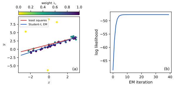
pp. 293–295 The likelihood \(\mathcal T(y\given\bm w^\T\bm x,\sigma^2,\nu)\) (6.165) has no missing data, but writing the Student distribution as a Gaussian scale mixture with a latent scale \(z_n\) per example makes EM applicable. The M step is weighted least squares with weights \(\lambda_n=\E[1/z_n]=(\nu+1)/(\nu+\delta_n)\), \(\delta_n=(y_n-\bm w^\T\bm x_n)^2/\sigma^2\) (6.168–6.170): large residuals get small weights.
Filling the gap 6.16: the Gaussian scale mixture, the posterior of the scale, and the weighted-least-squares M step pp. 293–295, (6.165)–(6.170)
Derivation
Scale mixture. Claim: \(\mathcal T(y\given\mu,\sigma^2,\nu)=\int_0^\infty\N(y\given\mu,\sigma^2z)\,\mathrm{IG}(z\given\tfrac\nu2,\tfrac\nu2)\mathrm dz\) (inverse-gamma with shape \(\nu/2\) and scale \(\nu/2\)). With \(\delta=(y-\mu)^2/\sigma^2\), the integrand is \((2\pi\sigma^2)^{-1/2}\frac{(\nu/2)^{\nu/2}}{\Gamma(\nu/2)}z^{-\frac{\nu+1}2-1}e^{-(\nu+\delta)/(2z)}\), and \(\int_0^\infty z^{-a-1}e^{-b/z}\mathrm dz=\Gamma(a)b^{-a}\) with \(a=\frac{\nu+1}2\), \(b=\frac{\nu+\delta}2\). Collecting, \(\frac{\Gamma(\frac{\nu+1}2)}{\Gamma(\frac\nu2)\sqrt{\pi\nu\sigma^2}}(1+\delta/\nu)^{-\frac{\nu+1}2}\), the Student density. (Numerical quadrature agrees to \(10^{-8}\).)
Posterior of the scale. The same integrand, as a function of \(z\), is proportional to \(z^{-\frac{\nu+1}2-1}e^{-(\nu+\delta)/(2z)}\), so \(z\given y\sim\mathrm{IG}(\frac{\nu+1}2,\frac{\nu+\delta}2)\) (6.169). If \(z\sim\mathrm{IG}(a,b)\) then \(1/z\sim\mathrm{Gamma}(a,\text{rate }b)\) with mean \(a/b\), hence \(\lambda_n=\E[1/z_n]=(\nu+1)/(\nu+\delta_n)\) (6.170).
M step. The complete-data log-likelihood is \(\sum_n\{-\tfrac12\log(2\pi z_n\sigma^2)-\frac{(y_n-\bm w^\T\bm x_n)^2}{2z_n\sigma^2}+\log\mathrm{IG}(z_n)\}\) (6.166–6.167). Taking the expectation, \(Q=-\frac1{2\sigma^2}\sum_n\lambda_n(y_n-\bm w^\T\bm x_n)^2-\tfrac N2\log\sigma^2+\const\) (the \(-\tfrac N2\log\sigma^2\) term is dropped in (6.168) when only \(\bm w\) is updated), a weighted least-squares problem: \(\bm w=(X^\T\Lambda X)^{-1}X^\T\Lambda\bm y\), \(\sigma^2=\frac1N\sum_n\lambda_n r_n^2\), \(\Lambda=\diag(\lambda_n)\). For \(\nu\) there is no closed form: ECME (6.5.6.5) maximises the observed likelihood over \(\nu\) with the other parameters fixed. Numerically, the EM iterates increase the Student log-likelihood monotonically and converge to the same optimum as a general-purpose optimiser run directly on the likelihood (fixed \(\nu\)); outliers receive weights below one fifth of the median weight.
6.5.6 Extensions to EM
pp. 295–297 Variational EM (6.5.6.1), hard EM (6.5.6.2), Monte Carlo EM and stochastic-approximation EM (6.5.6.3), generalised EM including gradient and quasi-Newton EM (6.5.6.4), ECM and ECME (6.5.6.5) and online EM (6.5.6.6) are all analysed through the identity of gap 6.14: every one preserves (or deliberately gives up) one of "the bound is tight" and "the bound increases".
S7.3 Conjugate duality (supplement)
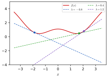
Supp. pp. 71–75 Conjugate duality builds linear lower bounds on a function, which is how variational bounds on awkward terms (such as the sigmoid in Bayesian logistic regression) are made. For any function \(f\) and slope \(\lambda\), \(L(x,\lambda)=\lambda^\T x-f^\ast(\lambda)\le f(x)\) (7.80), where the intercept \(f^\ast(\lambda)=\max_x\{\lambda^\T x-f(x)\}\) (7.83) is the conjugate (Fenchel transform; Legendre transform if \(f\) is differentiable): sliding the line of slope \(\lambda\) up until it touches \(f\) at \(x_\lambda\) (Figure S7.4).
S7.3.2–S7.3.3 Example: the exponential function; conjugate of a conjugate
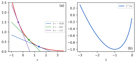
Supp. pp. 72–74 For \(f(x)=e^{-x}\), \(f^\dagger(\lambda)=-\lambda\log(-\lambda)+\lambda\) for \(\lambda<0\) (7.85), tight at \(x_\lambda=-\log(-\lambda)\) (7.88), and the conjugate of the conjugate returns \(e^{-x}\) (7.97).
S7.3.4 Bounds for the logistic (sigmoid) function
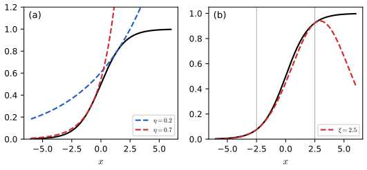
Supp. pp. 74–75 Exponential upper bound \(\sigma(x)\le\exp(\eta x-f^\dagger(\eta))\) with \(f^\dagger(\eta)\) the binary entropy (7.100–7.102), and the Jaakkola–Jordan quadratic lower bound \(\sigma(x)\ge\sigma(\xi)\exp\{(x-\xi)/2-\lambda(\xi)(x^2-\xi^2)\}\) (7.110) with \(\lambda(\xi)=\frac{\tanh(\xi/2)}{4\xi}=\frac{\sigma(\xi)-1/2}{2\xi}\) (7.107).
Filling the gap 6.17: conjugates, \(f^{\ast\ast}=f\), the exponential and quadratic bounds on the sigmoid, and a sign slip in (7.108) Supp. pp. 71–75, (7.80)–(7.110)
Derivation
Basic facts. \(f^\ast\) is a supremum of affine functions of \(\lambda\), hence convex. Directly from the definition, \(f(x)+f^\ast(\lambda)\ge\lambda^\T x\) (Fenchel–Young), i.e. (7.80). Maximising the left side's slack over \(\lambda\) gives \(f^{\ast\ast}(x)=\sup_\lambda\{\lambda^\T x-f^\ast(\lambda)\}\le f(x)\) (7.91). \(f^{\ast\ast}=f\) for convex \(f\). Assume \(f\) is convex, finite and differentiable (the general closed proper convex case follows from supporting hyperplanes; Rockafellar, 1970). Fix \(x_0\), \(\lambda_0=\nabla f(x_0)\). Convexity gives \(f(x)\ge f(x_0)+\lambda_0^\T(x-x_0)\) for all \(x\), i.e. \(\lambda_0^\T x-f(x)\le\lambda_0^\T x_0-f(x_0)\), so the maximum is attained at \(x_0\): \(f^\ast(\lambda_0)=\lambda_0^\T x_0-f(x_0)\). Hence \(f^{\ast\ast}(x_0)\ge\lambda_0^\T x_0-f^\ast(\lambda_0)=f(x_0)\), and with (7.91) equality. This is why a convex function is the upper envelope of its tangent lines (the epigraph is an intersection of half-spaces, Figure 7.5b of the book).
Exponential. \(J(x,\lambda)=\lambda x-e^{-x}\) has \(\partial_xJ=\lambda+e^{-x}\) (the printed (7.87) writes \(\lambda x\) in place of \(\lambda\)), zero at \(x_\lambda=-\log(-\lambda)\) (\(\lambda<0\)), where \(e^{-x_\lambda}=-\lambda\) and \(f^\dagger(\lambda)=-\lambda\log(-\lambda)+\lambda\) (7.89). Conversely \(f^{\ast\ast}(x)=\max_\lambda\{\lambda x+\lambda\log(-\lambda)-\lambda\}\): the derivative \(x+\log(-\lambda)=0\) gives \(\lambda=-e^{-x}\) and the value \(-xe^{-x}+xe^{-x}+e^{-x}=e^{-x}\) (7.97).
Sigmoid, upper bound. \(g=\log\sigma\) is concave (\(g''=-\sigma(1-\sigma)<0\)), so \(g(x)=\min_\eta\{\eta x-g^\dagger(\eta)\}\) with \(g^\dagger(\eta)=\min_x\{\eta x-g(x)\}\) (7.98–7.99). Stationarity \(\eta=g'(x)=1-\sigma(x)\) gives \(x=\log\frac{1-\eta}\eta\) and \(g^\dagger(\eta)=\eta\log\frac{1-\eta}\eta-\log(1-\eta)=-\eta\log\eta-(1-\eta)\log(1-\eta)\) (7.100), the binary entropy. Hence \(\log\sigma(x)\le\eta x-g^\dagger(\eta)\) for every \(\eta\in(0,1)\), with equality at \(\eta=1-\sigma(x)\), which is (7.101)–(7.102).
Sigmoid, quadratic lower bound. \(\log\sigma(x)=\tfrac x2-\log(e^{x/2}+e^{-x/2})=\tfrac x2+\phi(x^2)\) with \(\phi(y)=-\log(e^{\sqrt y/2}+e^{-\sqrt y/2})=-\log(2\cosh\tfrac{\sqrt y}2)\). This \(\phi\) has \(\phi'(y)=-\frac{\tanh(\sqrt y/2)}{4\sqrt y}\), which is increasing in \(y\) (because \(\tanh(u)/u\) decreases for \(u>0\)), so \(\phi\) is convex in \(y\) (7.103–7.105). A convex function lies above its tangent line at \(y=\xi^2\): \(\phi(y)\ge\phi(\xi^2)-\lambda(\xi)(y-\xi^2)\) with \(\lambda(\xi)=\frac{\tanh(\xi/2)}{4\xi}=\frac{\sigma(\xi)-1/2}{2\xi}\) (7.106–7.107). Therefore \(\log\sigma(x)\ge\tfrac x2-\lambda(\xi)x^2+\lambda(\xi)\xi^2-\log(2\cosh\tfrac\xi2)\) (7.109), and since \(\sigma(\xi)=e^{\xi/2}/(2\cosh\frac\xi2)\), exponentiating gives \(\sigma(x)\ge\sigma(\xi)\exp\{(x-\xi)/2-\lambda(\xi)(x^2-\xi^2)\}\) (7.110), tight at \(x=\pm\xi\) (the bound depends on \(x\) only through \(x^2\)).
Sign slip. With \(\eta=-\lambda(\xi)\) the conjugate in the variable \(y\) is \(f^\dagger(\lambda(\xi))=-\lambda(\xi)\xi^2-\phi(\xi^2)\); the printed (7.108) has \(+\lambda(\xi)\xi^2\), which is inconsistent with its own (7.109). All bounds were checked numerically on a fine grid: the upper bound holds for \(\eta\in\{0.05,\dots,0.95\}\) and the lower bound for several \(\xi\), and both are tight where claimed.
S7.1 Proximal methods (supplement)
Supp. pp. 55–70 Proximal methods use the proximal operator of a function instead of its gradient or Hessian. They apply directly to nonsmooth terms such as \(\ell_1\) penalties and constraints, and they decompose large problems. The first volume gives the \(\ell_1\) case in Section 8.6.
S7.1.1 Proximal operators
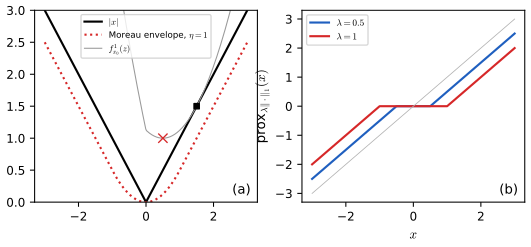
Supp. pp. 55–58 For convex \(f:\R^n\to\R\cup\{+\infty\}\), \(\prox_f(\bm x)=\argmin_{\bm z}\{f(\bm z)+\tfrac12\|\bm z-\bm x\|^2\}\) (7.2), unique because the objective is strongly convex; for the scaled function \(\prox_{\eta f}(\bm x)=\argmin_z\{f(z)+\frac1{2\eta}\|z-x\|^2\}\) (7.5). If \(f\) is the indicator of a convex set \(\mathcal C\), \(\prox_f\) is the Euclidean projection (7.3–7.4). The Moreau envelope is \(f^\eta(\bm x)=\min_z\{f(z)+\frac1{2\eta}\|z-x\|^2\}\) (7.9), a smooth lower bound of \(f\) with the same minimisers; the envelope of \(|x|\) is the Huber function. A prox step on a linearised \(f\) is the gradient step (7.12), on a quadratic model the regularised Newton step (7.14), and in general \(\prox_{\eta f}(\bm x)=\bm x-\eta\nabla f^\eta(\bm x)\) (7.16–7.17): a gradient step on the smoothed objective.
S7.1.2 Computing proximal operators
Supp. pp. 58–61 The Moreau decomposition \(\bm x=\prox_f(\bm x)+\prox_{f^\ast}(\bm x)\) (7.18) turns the prox of a norm into a projection onto the dual-norm ball, \(\prox_{\lambda\|\cdot\|}(\bm x)=\bm x-\lambda\,\mathrm{proj}_B(\bm x/\lambda)\) (7.21). Results: projection onto a box (7.22) and onto the nonnegative orthant \(x_+\) (7.23); soft thresholding for \(\ell_1\) (7.26); block soft thresholding \((1-\lambda/\|\bm x\|_2)_+\bm x\) for \(\ell_2\) (7.28); shrinkage \(\bm x/(1+\lambda)\) for \(\frac12\|\cdot\|^2\) (7.29) and \((I+\lambda A)^{-1}(\bm x-\lambda\bm b)\) for a quadratic (7.30); singular value thresholding for the nuclear norm (7.31); eigenvalue clipping for the PSD cone (7.32); the simplex projection \((\bm x-\nu\bm1)_+\) (7.33).
Filling the gap 6.18: the prox is firmly nonexpansive, the gradient of the Moreau envelope, the Moreau decomposition, and each closed form Supp. pp. 55–61, (7.2)–(7.33)
Derivation
Characterisation and nonexpansiveness. \(\bm z=\prox_f(\bm x)\) iff \(\bm 0\in\partial f(\bm z)+\bm z-\bm x\), i.e. \(\bm x-\bm z\in\partial f(\bm z)\) (optimality of a strongly convex problem). For \(\bm z=\prox_f(\bm x)\), \(\bm z'=\prox_f(\bm x')\), monotonicity of the subdifferential gives \(\langle(\bm x-\bm z)-(\bm x'-\bm z'),\bm z-\bm z'\rangle\ge0\), so \(\|\bm z-\bm z'\|^2\le\langle\bm x-\bm x',\bm z-\bm z'\rangle\le\|\bm x-\bm x'\|\|\bm z-\bm z'\|\): \(\prox_f\) is nonexpansive (indeed firmly), hence continuous.
Gradient of the envelope (7.16). Let \(\bm z_x=\prox_{\eta f}(\bm x)\). By definition \(f^\eta(\bm y)\le f(\bm z_x)+\frac1{2\eta}\|\bm z_x-\bm y\|^2\) with equality at \(\bm y=\bm x\); subtracting, \(f^\eta(\bm y)-f^\eta(\bm x)\le\frac1{2\eta}(\|\bm z_x-\bm y\|^2-\|\bm z_x-\bm x\|^2)=\frac1\eta\langle\bm x-\bm z_x,\bm y-\bm x\rangle+\frac1{2\eta}\|\bm y-\bm x\|^2\). Exchanging roles, \(f^\eta(\bm y)-f^\eta(\bm x)\ge\frac1\eta\langle\bm x-\bm z_y,\bm y-\bm x\rangle-\frac1{2\eta}\|\bm y-\bm x\|^2\). Since \(\bm z_y\to\bm z_x\) as \(\bm y\to\bm x\) (nonexpansiveness), \(f^\eta\) is differentiable with \(\nabla f^\eta(\bm x)=(\bm x-\bm z_x)/\eta\), even when \(f\) is not (7.16), so \(\prox_{\eta f}(\bm x)=\bm x-\eta\nabla f^\eta(\bm x)\) (7.17). For \(f=|x|\): \(f^1(x_0)=|0.5|+\frac12(1)^2=1.0\) at \(x_0=1.5\), the worked example in the text, and \(f^\eta\) is Huber, \(x^2/2\eta\) for \(|x|\le\eta\) and \(|x|-\eta/2\) beyond.
Moreau decomposition (7.18). \(\bm z=\prox_f(\bm x)\iff\bm x-\bm z\in\partial f(\bm z)\iff\bm z\in\partial f^\ast(\bm x-\bm z)\) (the conjugate subgradient relation, \(\bm u\in\partial f(\bm z)\iff\bm z\in\partial f^\ast(\bm u)\) for closed convex \(f\)) \(\iff\bm x-(\bm x-\bm z)\in\partial f^\ast(\bm x-\bm z)\iff\bm x-\bm z=\prox_{f^\ast}(\bm x)\). For a norm \(f=\|\cdot\|\), \(f^\ast=\ind_B\), \(B\) the dual unit ball (7.19–7.20), and \((\lambda f)^\ast=\ind_{\lambda B}\), so \(\prox_{\lambda f}(\bm x)=\bm x-\mathrm{proj}_{\lambda B}(\bm x)=\bm x-\lambda\mathrm{proj}_B(\bm x/\lambda)\) (7.21).
Closed forms. \(\ell_1\): the dual ball is the \(\ell_\infty\) ball, whose projection is clipping to \([-\lambda,\lambda]\), so \(\prox_{\lambda\|\cdot\|_1}(x)_i=x_i-\mathrm{clip}(x_i,-\lambda,\lambda)=\sign(x_i)(|x_i|-\lambda)_+\). The case conditions are, correctly, \(x-\lambda\) if \(x\ge\lambda\), \(0\) if \(|x|\le\lambda\), \(x+\lambda\) if \(x\le-\lambda\) (the printed (7.25) has the second condition as \(|x|\ge\lambda\) and the third as \(x\le\lambda\)); directly, the scalar optimality condition \(x-z\in\lambda\partial|z|\) gives these three cases. \(\ell_2\): the dual ball is the Euclidean ball, \(\mathrm{proj}_B(\bm u)=\bm u/\max(1,\|\bm u\|)\), giving \((1-\lambda/\|\bm x\|)_+\bm x\) (7.28). Squared norm and quadratics: setting the gradient of \(\lambda(\frac12\bm z^\T A\bm z+\bm b^\T\bm z)+\frac12\|\bm z-\bm x\|^2\) to zero gives (7.30). Nuclear norm: the dual norm is the spectral norm, so the prox is \(A-\mathrm{proj}_{\{\sigma_{\max}\le\lambda\}}(A)\); the projection clips the singular values at \(\lambda\) (by von Neumann's trace inequality \(\langle A,X\rangle\le\sum\sigma_i(A)\sigma_i(X)\), the minimiser shares the singular vectors of \(A\); von Neumann, 1937), leaving \(\sum_i(\sigma_i-\lambda)_+\bm u_i\bm v_i^\T\) (7.31). PSD cone: for symmetric \(A\) and PSD \(P\), the Hoffman–Wielandt inequality \(\|A-P\|_F^2\ge\sum_i(\lambda_i(A)-\lambda_i(P))^2\ge\sum_i(\lambda_i(A)-(\lambda_i(A))_+)^2\), attained by eigenvalue clipping (7.32). Simplex: the KKT conditions of \(\min\frac12\|\bm z-\bm x\|^2\) s.t. \(\bm z\ge0\), \(\bm1^\T\bm z=1\) give \(z_i=(x_i-\nu)_+\) for the multiplier \(\nu\) of the equality; \(\nu\mapsto\sum_i(x_i-\nu)_+\) is continuous and strictly decreasing where positive, so the root is unique and found by bisection or exactly by sorting: with \(u_1\ge\dots\ge u_n\), \(\nu=(\sum_{i\le\rho}u_i-1)/\rho\) where \(\rho=\max\{k:u_k-(\sum_{i\le k}u_i-1)/k>0\}\) (7.33). All closed forms were compared with brute-force minimisation (a grid for scalars, Nelder–Mead for vectors, SLSQP for the simplex).
S7.1.3 Proximal point methods (PPM)
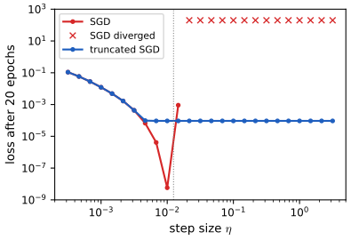
Supp. pp. 61–63 \(\bm\theta_{t+1}=\prox_{\eta_tL}(\bm\theta_t)=\argmin_\theta\{L(\bm\theta)+\frac1{2\eta_t}\|\bm\theta-\bm\theta_t\|^2\}\) (7.34). Applied to the linearisation \(\hat L_t(\bm\theta)=L_t(\bm\theta_t)+\bm g_t^\T(\bm\theta-\bm\theta_t)\) it is exactly SGD (7.35–7.37). Keeping a known lower bound of the loss, \(\hat L_t=\max\{L_t(\bm\theta_t)+\bm g_t^\T(\bm\theta-\bm\theta_t),L_{\min}\}\) (7.38), gives truncated steps \(\bm\theta_{t+1}=\bm\theta_t-\min\{\eta_t,L_t/\bm g_t^\T A_t^{-1}\bm g_t\}\bm g_t\) (7.40; scaled by AdaGrad's \(A_t\) in the book), which are stable for any learning rate (Figure 7.2). The stochastic and incremental versions (7.41) are more stable than SGD; for least squares the incremental PPM is the Kalman filter.
S7.1.4 Mirror descent
Supp. pp. 63–66 Replace the Euclidean proximity term by a Bregman divergence \(D_\psi(\bm\theta,\bm\theta')=\psi(\bm\theta)-\psi(\bm\theta')-\nabla\psi(\bm\theta')^\T(\bm\theta-\bm\theta')\) (7.42) of a strongly convex mirror map \(\psi\): \(\bm\theta_{t+1}=\argmin_\theta\{\eta_t\bm g_t^\T\bm\theta+D_\psi(\bm\theta,\bm\theta_t)\}\) (7.43–7.45).
Filling the gap 6.19: PPM descent and rate, the truncated step and its stability for every learning rate, and mirror descent in primal and dual form Supp. pp. 61–66, (7.34)–(7.50)
Derivation
PPM. Let \(\bm\theta^+=\prox_{\eta L}(\bm\theta)\) for convex \(L\). The prox objective is \(\frac1\eta\)-strongly convex and minimised at \(\bm\theta^+\), so for every \(\bm u\): \(L(\bm\theta^+)+\frac1{2\eta}\|\bm\theta^+-\bm\theta\|^2\le L(\bm u)+\frac1{2\eta}\|\bm u-\bm\theta\|^2-\frac1{2\eta}\|\bm u-\bm\theta^+\|^2\). With \(\bm u=\bm\theta\) this shows \(L(\bm\theta^+)\le L(\bm\theta)-\frac1{2\eta}\|\bm\theta^+-\bm\theta\|^2\) (descent for any \(\eta>0\), no smoothness needed); with \(\bm u=\bm\theta^\ast\), summing over \(t\) and telescoping, \(\sum_t\eta_t(L(\bm\theta_{t+1})-L^\ast)\le\frac12\|\bm\theta_0-\bm\theta^\ast\|^2\), so by monotonicity \(L(\bm\theta_k)-L^\ast\le\|\bm\theta_0-\bm\theta^\ast\|^2/(2\sum_{t<k}\eta_t)\): the rate improves with larger steps, and arbitrarily large steps are admissible (at the price of an expensive subproblem).
GD is PPM on the linearisation. The gradient of \(L_t(\bm\theta_t)+\bm g_t^\T(\bm\theta-\bm\theta_t)+\frac1{2\eta}\|\bm\theta-\bm\theta_t\|^2\) is \(\bm g_t+(\bm\theta-\bm\theta_t)/\eta\), zero at \(\bm\theta_t-\eta\bm g_t\) (7.37).
Truncated step (7.40, \(A_t=I\), \(L_{\min}=0\)). Minimise \(m(\bm\theta)=\max\{L_t+\bm g^\T(\bm\theta-\bm\theta_t),0\}+\frac1{2\eta}\|\bm\theta-\bm\theta_t\|^2\), a convex function minimised along \(-\bm g\) by symmetry of the proximity term, \(\bm\theta=\bm\theta_t-s\bm g\), \(s\ge0\). On the linear branch the minimiser is \(s=\eta\), valid iff the model value \(L_t-\eta\|\bm g\|^2\ge0\), i.e. \(\eta\le L_t/\|\bm g\|^2\). Otherwise the minimiser sits at the kink, \(L_t-s\|\bm g\|^2=0\), \(s=L_t/\|\bm g\|^2\). So \(s=\min\{\eta,L_t/\|\bm g\|^2\}\), which is the footnote's case analysis.
Stability for any \(\eta\). Let the loss \(L_t\ge0\) be convex with an interpolating point \(\bm\theta^\ast\), \(L_t(\bm\theta^\ast)=0\), and \(\bm e=\bm\theta_t-\bm\theta^\ast\). Convexity gives \(\bm g^\T\bm e\ge L_t(\bm\theta_t)-L_t(\bm\theta^\ast)=L_t\). Then \(\|\bm e-s\bm g\|^2=\|\bm e\|^2-2s\bm g^\T\bm e+s^2\|\bm g\|^2\le\|\bm e\|^2-2sL_t+s\cdot s\|\bm g\|^2\le\|\bm e\|^2-sL_t\), using \(s\|\bm g\|^2\le L_t\). So the distance to the interpolant never increases, whatever \(\eta\) is, whereas plain SGD (\(s=\eta\)) has \(\|\bm e-\eta\bm g\|^2\) potentially much larger than \(\|\bm e\|^2\) for large \(\eta\) and diverges (Figure 7.2 below). For a convex nonnegative loss that is not interpolated the truncated model is still a lower bound, which is the book's "stable for any learning rate (under technical conditions)".
Mirror descent. Dropping terms that do not involve \(\bm\theta\), (7.45) is \(\min\{\bm\theta^\T(\eta\bm g_t-\nabla\psi(\bm\theta_t))+\psi(\bm\theta)\}\); at an interior minimiser \(\nabla\psi(\bm\theta_{t+1})=\nabla\psi(\bm\theta_t)-\eta\bm g_t\), i.e. gradient descent in the dual variable \(\bm z=\nabla\psi(\bm\theta)\), mapped back by \(\bm\theta=\nabla\psi^\ast(\bm z)\) because \(\nabla\psi^\ast=(\nabla\psi)^{-1}\) for a strictly convex differentiable \(\psi\) (7.50–7.54). With \(\psi=\frac12\|\cdot\|^2\) (\(D_\psi=\frac12\|\bm\theta-\bm\theta'\|^2\)) this is ordinary gradient descent (7.46–7.49). On the simplex with \(\psi(\bm\theta)=\sum_i\theta_i\log\theta_i\): for \(\bm\theta,\bm\theta'\) with \(\sum\theta_i=\sum\theta'_i=1\), \(D_\psi=\sum\theta_i\log\frac{\theta_i}{\theta_i'}-\sum(\theta_i-\theta_i')=\KL(\bm\theta\|\bm\theta')\). The Lagrangian of \(\min\{\eta\bm g^\T\bm\theta+\KL(\bm\theta\|\bm\theta_t)\}\) s.t. \(\bm1^\T\bm\theta=1\) gives \(\log(\theta_i/\theta_{t,i})=-\eta g_i-\lambda-1\), so \(\theta_{t+1,i}\propto\theta_{t,i}e^{-\eta g_i}\), the exponential weights algorithm (checked against a constrained solver). Finally, on an exponential-family \(q\), mirror descent in the mean parameters with \(\psi=-H\) is natural-gradient descent in the natural parameters (7.1.4.4; Raskutti and Mukherjee, 2015), consistent with Gap 6.11.
S7.1.5 Proximal gradient method
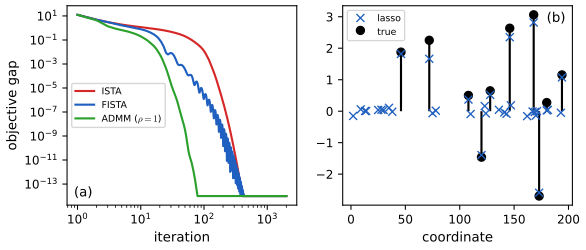
Supp. pp. 66–67 For \(L=L_s+L_r\) with \(L_s\) smooth convex and \(L_r\) convex, possibly nonsmooth: \(\bm\theta_{t+1}=\prox_{\eta_tL_r}(\bm\theta_t-\eta_t\nabla L_s(\bm\theta_t))\) (7.51), projected gradient descent if \(L_r=\ind_{\mathcal C}\); with Nesterov extrapolation (7.52–7.53). For the lasso \(L_s=\frac12\|X\bm\theta-\bm y\|^2\), \(L_r=\lambda\|\bm\theta\|_1\) this is ISTA (7.56), and FISTA is the accelerated version.
S7.1.6 Alternating direction method of multipliers (ADMM)
Supp. pp. 67–70 For \(L_s(\bm x)+L_r(\bm z)\) with both terms possibly nonsmooth, split the variable, \(\min L_s(\bm x)+L_r(\bm z)\) s.t. \(\bm x-\bm z=0\) (7.57), and alternate minimisation of the augmented Lagrangian \(L_\rho=L_s(\bm x)+L_r(\bm z)+\bm y^\T(\bm x-\bm z)+\frac\rho2\|\bm x-\bm z\|^2\) (7.58) with a dual ascent step (7.59–7.61). In scaled form (\(\bm u=\bm y/\rho\), \(\lambda=1/\rho\)): \(\bm x_{t+1}=\prox_{\lambda L_s}(\bm z_t-\bm u_t)\), \(\bm z_{t+1}=\prox_{\lambda L_r}(\bm x_{t+1}+\bm u_t)\), \(\bm u_{t+1}=\bm u_t+\bm x_{t+1}-\bm z_{t+1}\) (7.66–7.68).
Filling the gap 6.20: the ISTA rate, ADMM in scaled form, and robust PCA by ADMM Supp. pp. 66–70, (7.51)–(7.74)
Derivation
One-step inequality for proximal gradient. Let \(L_s\) have \(\ell\)-Lipschitz gradient, step \(1/\ell\), \(\bm\theta^+=\prox_{L_r/\ell}(\bm\theta-\nabla L_s(\bm\theta)/\ell)\), \(F=L_s+L_r\). The descent lemma gives \(L_s(\bm\theta^+)\le L_s(\bm\theta)+\langle\nabla L_s,\bm\theta^+-\bm\theta\rangle+\frac\ell2\|\bm\theta^+-\bm\theta\|^2\). Since \(\bm\theta^+\) minimises the \(\ell\)-strongly convex \(L_r(\bm z)+\langle\nabla L_s,\bm z-\bm\theta\rangle+\frac\ell2\|\bm z-\bm\theta\|^2\), for every \(\bm u\): \(L_r(\bm\theta^+)+\langle\nabla L_s,\bm\theta^+-\bm\theta\rangle+\frac\ell2\|\bm\theta^+-\bm\theta\|^2\le L_r(\bm u)+\langle\nabla L_s,\bm u-\bm\theta\rangle+\frac\ell2\|\bm u-\bm\theta\|^2-\frac\ell2\|\bm u-\bm\theta^+\|^2\). Adding, and using convexity \(L_s(\bm\theta)+\langle\nabla L_s,\bm u-\bm\theta\rangle\le L_s(\bm u)\), \[ F(\bm\theta^+)\le F(\bm u)+\tfrac\ell2\big(\|\bm u-\bm\theta\|^2-\|\bm u-\bm\theta^+\|^2\big). \] With \(\bm u=\bm\theta\): \(F(\bm\theta^+)\le F(\bm\theta)\) (ISTA descends monotonically). With \(\bm u=\bm\theta^\ast\) and telescoping over \(t=0,\dots,k-1\), \(\sum_t(F(\bm\theta_{t+1})-F^\ast)\le\frac\ell2\|\bm\theta_0-\bm\theta^\ast\|^2\), so \(F(\bm\theta_k)-F^\ast\le\frac{\ell\|\bm\theta_0-\bm\theta^\ast\|^2}{2k}\): an \(O(1/k)\) rate. FISTA's extrapolation improves this to \(F(\bm\theta_k)-F^\ast\le2\ell\|\bm\theta_0-\bm\theta^\ast\|^2/(k+1)^2\) (Beck and Teboulle, 2009; proof omitted). Both bounds were verified on a lasso problem (Figure x6.b), together with agreement of ISTA, FISTA and ADMM with coordinate descent to \(10^{-4}\).
ADMM, scaled form. Completing the square, \(\bm y^\T(\bm x-\bm z)+\frac\rho2\|\bm x-\bm z\|^2=\frac\rho2\|\bm x-\bm z+\bm u\|^2-\frac\rho2\|\bm u\|^2\) with \(\bm u=\bm y/\rho\). Minimising over \(\bm x\) with \(\bm z,\bm u\) fixed gives \(\argmin_x\{L_s(\bm x)+\frac\rho2\|\bm x-(\bm z-\bm u)\|^2\}=\prox_{L_s/\rho}(\bm z-\bm u)\), over \(\bm z\) similarly \(\prox_{L_r/\rho}(\bm x+\bm u)\), and the dual step \(\bm y_{t+1}=\bm y_t+\rho(\bm x_{t+1}-\bm z_{t+1})\) is \(\bm u_{t+1}=\bm u_t+\bm x_{t+1}-\bm z_{t+1}\): (7.66)–(7.68). Under convexity the objective converges at rate \(O(1/k)\) and the residual \(\bm x-\bm z\to0\) (Boyd et al., 2011). For the lasso, \(\bm x\) solves \((A^\T A+\rho I)\bm x=A^\T\bm b+\rho(\bm z-\bm u)\) and \(\bm z\) is a soft-thresholding at \(\lambda/\rho\).
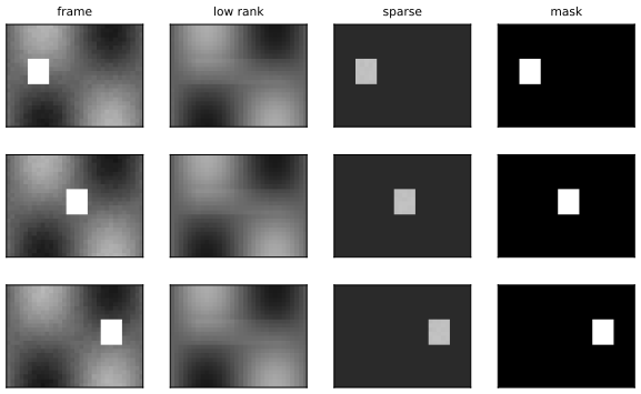
Robust PCA. The problem \(\min\|A-L-S\|_F^2+\gamma_L\|L\|_\ast+\gamma_S\|S\|_1\) (7.70) is cast as \(\min\sum_j\gamma_j\phi_j(X_j)\) s.t. \(\sum_jX_j=A\) with \(X_1=L\), \(X_2=S\), \(X_3=A-L-S\) (7.69, 7.71). ADMM with the split \(L_s=\sum_j\gamma_j\phi_j\), \(L_r=\ind_{\{\sum X_j=A\}}\) uses the projection onto the constraint set, \((X_j)\mapsto(X_j)-\bar X+A/J\) (7.74), where \(\bar X\) is the average of the \(J\) blocks, giving \(X_{j,t+1}=\prox_{\eta\gamma_j\phi_j}(X_{j,t}-\bar X_t+A/J-U_t)\), \(U_{t+1}=U_t+\bar X_{t+1}-A/J\) (7.72–7.73; the book writes \(A/N\) in (7.72), which should be \(A/J\) as in (7.73)). The prox's are singular value thresholding (nuclear norm), soft thresholding (\(\ell_1\)) and shrinkage \(X/(1+2\eta)\) (squared Frobenius norm). The blocks are updated in parallel.
6.6 Bayesian optimization
pp. 297–304 Bayesian optimisation (BayesOpt) maximises an expensive black-box \(f:\mathcal X\to\R\) using a probabilistic surrogate built from the evaluations so far. Unlike a bandit, which pays for every action (cumulative regret), BayesOpt cares only about the final solution (simple regret); unlike active learning, it wants the maximum rather than the whole function.
6.6.1 Sequential model-based optimization
pp. 298 Algorithm 6.5: start from \(\mathcal D_0\) (random or space-filling queries), then repeat: choose \(\bm x_{n+1}=\argmax_{\bm x}\alpha(\bm x;\mathcal D_n)\), observe \(y_{n+1}=f(\bm x_{n+1})+\epsilon\), augment \(\mathcal D_n\), update \(p(f\given\mathcal D_n)\). Two ingredients are needed: a surrogate and an acquisition function.
6.6.2 Surrogate functions
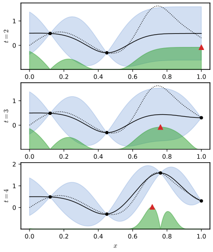
pp. 298–300 Gaussian processes give \(p(f(\bm x)\given\mathcal D_n)=\N(\mu_n(\bm x),\sigma_n^2(\bm x))\) in closed form (Section 17.2.2 of the first volume): with kernel matrix \(K\), \(\bm k(\bm x)=(k(\bm x,\bm x_i))_i\) and noise \(\sigma_y^2\), \(\mu_n(\bm x)=\bm k^\T(K+\sigma_y^2I)^{-1}\bm y\), \(\sigma_n^2(\bm x)=k(\bm x,\bm x)-\bm k^\T(K+\sigma_y^2I)^{-1}\bm k\). Cost \(O(n^3)\); the kernel matters. Alternatives: Bayesian neural networks, ensembles of random forests (which handle conditional hyperparameters).
6.6.3 Acquisition functions
pp. 300–303 The acquisition \(\alpha(\bm x\given\mathcal D_n)=\E_{p(y\given x,\mathcal D_n)}[U(\bm x,y;\mathcal D_n)]\) is an expected utility. With \(M_n=\max_iy_i\) the incumbent and \(\gamma_n(\bm x,\tau)=(\mu_n(\bm x)-\tau)/\sigma_n(\bm x)\): probability of improvement \(\alpha_{PI}=\Phi(\gamma_n(\bm x,M_n))\) (6.174–6.175); expected improvement \(\alpha_{EI}=(\mu_n-M_n)\Phi(\gamma)+\sigma_n\varphi(\gamma)\) (6.176–6.177), or by Monte Carlo \(\frac1S\sum_s\max(\mu_n^s(\bm x)-M_n,0)\) (6.178); upper confidence bound \(\mu_n+\beta_n\sigma_n\); Thompson sampling \(\bm x_{n+1}=\argmax_{\bm x}f_{\tilde\theta}(\bm x)\) for a posterior sample \(\tilde\theta\) (6.179–6.180); entropy search \(\alpha_{ES}=H(\bm x^\ast\given\mathcal D_n)-\E_y H(\bm x^\ast\given\mathcal D_n\cup\{(\bm x,y)\})\) (6.181–6.182), rewritten as predictive entropy search (6.183); and the knowledge gradient (6.184–6.186), which looks one step ahead at the posterior maximum.
Filling the gap 6.21: the closed forms of PI and EI, why EI balances exploration and exploitation, Thompson sampling, and the entropy-search identity pp. 300–302, (6.174)–(6.183)
Derivation
PI and EI. Under the GP, \(f(\bm x)=\mu+\sigma\epsilon\), \(\epsilon\sim\N(0,1)\), \(\gamma=(\mu-M)/\sigma\). \(\Pr(f>M)=\Pr(\epsilon>-\gamma)=\Phi(\gamma)\) (6.174). For EI, \((f-M)_+=\sigma(\epsilon+\gamma)_+\) and \[ \E(f-M)_+=\sigma\int_{-\gamma}^\infty(\epsilon+\gamma)\varphi(\epsilon)\mathrm d\epsilon=\sigma\big[\varphi(\gamma)+\gamma(1-\Phi(-\gamma))\big]=\sigma[\gamma\Phi(\gamma)+\varphi(\gamma)], \] using \(\int_{-\gamma}^\infty\epsilon\varphi(\epsilon)\mathrm d\epsilon=\varphi(\gamma)\) (since \(\varphi'=-\epsilon\varphi\)): (6.177). Both closed forms agree with Monte Carlo to \(2\times10^{-3}\) with \(3\times10^6\) draws.
Exploration against exploitation. \(\partial\alpha_{EI}/\partial\mu=\Phi(\gamma)>0\) and \(\partial\alpha_{EI}/\partial\sigma=\varphi(\gamma)>0\): EI increases both with a higher predicted mean (the first term of (6.177), exploitation) and with more uncertainty (the second, exploration). In a noise-free problem at a queried point \(\sigma=0\) and \(\mu=y\le M\), so \(\alpha_{EI}=0\) (and \(\alpha_{PI}=0\)): queried points are never repeated. PI uses only the sign of the improvement and so exploits near the incumbent, as the demonstration shows (PI queries a run of neighbouring grid points). The UCB \(\mu+\beta\sigma\) makes the trade-off explicit through \(\beta\).
Thompson sampling. If \(\tilde f\) is a draw from \(p(f\given\mathcal D_n)\), then \(\bm x=\argmax\tilde f\) has exactly the posterior law of the maximiser \(\bm x^\ast\), i.e. density \(\alpha(\bm x)=\Pr(\bm x=\argmax f)\) (6.179); a single draw therefore selects a query with probability equal to the posterior probability that it is the optimum. (Checked on three independent Gaussian arms: the empirical frequency of each arm being the maximum matches the exact integral \(\int\varphi_i\prod_{j\ne i}\Phi_j\) to \(4\times10^{-3}\).)
Entropy search. The expected gain \(\alpha_{ES}=H(\bm x^\ast\given\mathcal D)-\E_yH(\bm x^\ast\given\mathcal D,y)=I(\bm x^\ast;y\given\mathcal D,\bm x)\) is a mutual information, which is symmetric: \(I(\bm x^\ast;y)=H(y)-\E_{\bm x^\ast}H(y\given\bm x^\ast)\), i.e. (6.183). The right-hand side needs entropies of the one-dimensional predictive distribution only, and the expectation over \(\bm x^\ast\) can be approximated by Thompson samples. (Checked on a random discrete joint distribution: both sides agree to rounding.)
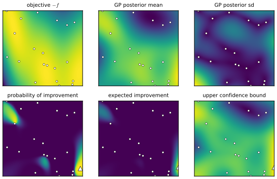
6.6.4 Other issues
pp. 303–304 Optimising the (multimodal) acquisition function is itself a hard subproblem (multi-start BFGS, the cross-entropy method, evolutionary search); parallel (batch) queries, conditional hyperparameters (tree-structured search spaces), multi-fidelity surrogates and early stopping, and unknown constraints (weighted EI, \(\alpha_{wEI}=\alpha_{EI}\,h(\bm x;\mathcal D_n)\) with \(h\) the feasibility probability) are described but not derived in the book.
6.7 Derivative-free optimization
pp. 304–314 Derivative-free optimisation (DFO) uses only function values. Bayesian optimisation is for expensive functions; cheap functions allow stochastic local search and population-based methods.
6.7.1 Local search
pp. 304–307 In a discrete space, hill climbing moves to the best neighbour \(\bm x_{t+1}=\argmax_{\bm x\in\mathrm{nbr}(\bm x_t)}L(\bm x)\) (6.187). On 8-queens (neighbours: move one queen within its column, \(8\times7=56\) neighbours) it gets stuck at a local maximum 86% of the time, taking about 4 steps when it succeeds and 3 when it fails. Stochastic local search samples uphill neighbours; random restarts repeat from random starts; tabu search (Algorithm 6.6) takes the best non-tabu neighbour, even if worse, and keeps a list of the \(\tau\) most recent states; random search draws points uniformly and beats grid search for hyperparameters because few of them matter (Figure 6.12).
Filling the gap 6.22: expected cost of random restarts, the search statistics on 8-queens, and why random search beats grid search pp. 305–307
Derivation
Random restarts. Each restart is an independent run that succeeds with probability \(p\) after on average \(N_1\) steps, or fails after on average \(N_0\) steps. The number of failures before the first success is geometric with mean \((1-p)/p=R-1\) where \(R=1/p\) is the expected number of runs. By Wald's identity the expected total number of steps is \(\E[\#\text{failures}]N_0+N_1=N_1+(R-1)N_0\). With the book's \(p\approx0.14\), \(N_1=4\), \(N_0=3\) this is \(4+6.1\times3\approx22\) (the book rounds \(R\) to 7 and gets 22). In the code, 2500 random starts give a success rate 0.134, 4.1 steps on success and 3.1 on failure, and the average total over 600 restart campaigns is 22.0 against the formula's 22.4 (Figure x6.a). The expected number of steps depends on the neighbourhood and the tie breaking; with random tie breaking this is the figure.
Tabu search. My implementation (best non-tabu neighbour; \(\tau=40\) most recent states tabu; stop after 60 steps without improvement) solves every one of 250 random 8-queens instances, against the 94% the book quotes for the variant in the literature; the parameters \(\tau\) and \(c_{\max}\) set the exploration, so the success rate is a property of the variant.
Random against grid search. A random search evaluating \(n\) uniform points hits the best \(q\)-fraction of the space with probability \(1-(1-q)^n\) (independent draws), so 59 draws reach the best 5% with probability \(1-0.95^{59}=0.951\), whatever the dimension (confirmed by simulation: 0.9513). A grid with \(k\) values per axis in \(d\) dimensions uses \(n=k^d\) evaluations but only \(k=n^{1/d}\) distinct values of each coordinate. If the objective depends on only \(d_{\rm eff}<d\) of the coordinates, the grid effectively tries \(n^{d_{\rm eff}/d}\) distinct settings of the ones that matter against \(n\) for random search (Figure 6.12: 3 distinct values of the important parameter against 9, and the best value found improves faster for random search at every budget).
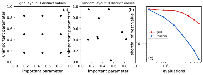
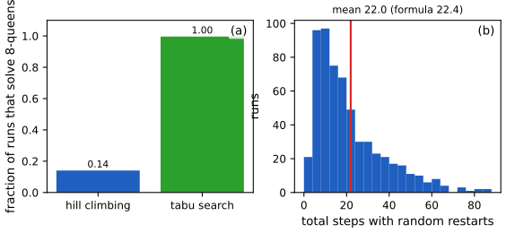
6.7.2–6.7.3 Simulated annealing and evolutionary algorithms
pp. 307–310 Simulated annealing converts the energy to \(p(\bm x)\propto e^{-E(\bm x)}\) and uses Metropolis–Hastings with decreasing temperature (Section 12.9.1 of the book). An evolutionary algorithm keeps a population of \(K\) candidates, with selection (truncation, tournament, fitness-proportionate or "regularised" age-based), recombination (crossover) and mutation; genetic algorithms use bit-string crossover (Figures 6.13, 6.14), genetic programming uses trees (6.15), surrogate-assisted EAs replace the objective by a model, memetic algorithms add local search. The figures 6.13–6.15 are hand-drawn schematics.
6.7.4 Estimation of distribution (EDA) algorithms
pp. 310–312 An EDA replaces the implicit density model of a population by an explicit one: sample \(K'\) candidates from \(p(\bm x\given\bm\theta_t)\), keep the best \(K\) (truncation selection), fit \(p(\bm x\given\bm\theta_{t+1})\) to them by maximum likelihood. For bit strings with fitness \(\sum_dx_d\) (one-max) and a factorised Bernoulli model this is UMDA; the incremental version \(\hat\theta_{d,t+1}=(1-\eta_t)\hat\theta_{d,t}+\eta_t\theta_{d,t}\) is PBIL (6.188); a multivariate Gaussian gives EMNA; Bayes nets give BOA (Figure 6.16).
6.7.5–6.7.6 Cross-entropy method and evolutionary strategies
pp. 312–314 The cross-entropy method (CEM) is the EDA with a Gaussian: \(\bm\mu_{t+1},\Sigma_{t+1}\) are the empirical mean and covariance of the elite samples; the differentiable CEM replaces top-\(K\) by a soft projection (6.189). Evolution strategies maximise the smoothed objective \(L(\bm\theta)=\E_{p(\bm x\given\bm\theta)}f(\bm x)\) by gradient ascent with the score-function estimator \(\nabla_\theta L=\E[f(\bm x)\nabla_\theta\log p(\bm x\given\bm\theta)]\) (6.190); for a Gaussian, \(\nabla_\mu\log p=\Sigma^{-1}(\bm x-\bm\mu)\) and \(\nabla_\Sigma\log p=\tfrac12\Sigma^{-1}(\bm x-\bm\mu)(\bm x-\bm\mu)^\T\Sigma^{-1}-\tfrac12\Sigma^{-1}\); with the isotropic \(\N(\bm\mu,\sigma^2I)\), \(\nabla_\mu L=\frac1\sigma\E_{\bm\epsilon}[f(\bm\mu+\sigma\bm\epsilon)\bm\epsilon]\), reducing the variance with mirrored samples \(\pm\bm\epsilon\). Natural evolution strategies use the natural gradient (Section 6.4); CMA-ES weights the elite by rank and updates the covariance through evolution paths, approximating the natural gradient of \(L\).
Filling the gap 6.23: EDA = maximum likelihood on the elite set (UMDA, CEM), the isotropic ES gradient and why mirrored sampling helps, and natural evolution strategies pp. 310–314, (6.188)–(6.190)
Derivation
EDA is cross-entropy minimisation. For the elite set \(S^\ast\), the empirical distribution is \(\hat p=\frac1{|S^\ast|}\sum_{x\in S^\ast}\delta_x\). Then \(\argmax_\theta\sum_{x\in S^\ast}\log p(x\given\theta)=\argmin_\theta\{-\E_{\hat p}\log p(x\given\theta)\}=\argmin_\theta\KL(\hat p\|p_\theta)\) (the entropy of \(\hat p\) does not depend on \(\theta\)), the cross entropy of the text. For a product of Bernoullis the maximiser of \(\sum_x\sum_d[x_d\log\theta_d+(1-x_d)\log(1-\theta_d)]\) is \(\theta_d\) = the fraction of elite samples with bit \(d\) on (UMDA); for a Gaussian it is the elite sample mean and the (biased) elite sample covariance (Section 4.2.6), which is CEM. PBIL (6.188) is the convex combination of the old and the MLE parameters. The truncation selection makes the fitness threshold rise with \(t\), so the model concentrates: on one-max with \(D=30\), the model parameters tend to 1 within 40 generations.
Isotropic ES gradient. For \(\bm x=\bm\mu+\sigma\bm\epsilon\), \(\nabla_\mu\log\N(\bm x\given\bm\mu,\sigma^2I)=(\bm x-\bm\mu)/\sigma^2=\bm\epsilon/\sigma\), so (6.190) is \(\nabla_\mu L=\frac1\sigma\E[f(\bm\mu+\sigma\bm\epsilon)\bm\epsilon]\). By Bonnet's theorem (Gap 6.4) this also equals \(\E[\nabla f(\bm\mu+\sigma\bm\epsilon)]\), the gradient of the Gaussian-smoothed function; for \(f(x)=x^4\), \(L=\mu^4+6\mu^2\sigma^2+3\sigma^4\) and \(\nabla_\mu L=4\mu^3+12\mu\sigma^2\), confirmed by Monte Carlo.
Mirrored sampling. Using the pair \(\pm\bm\epsilon\) gives the estimator \(\frac1{2\sigma}[f(\bm\mu+\sigma\bm\epsilon)-f(\bm\mu-\sigma\bm\epsilon)]\bm\epsilon\), unbiased because \(\bm\epsilon\) and \(-\bm\epsilon\) have the same law, and free of the term \(f(\bm\mu)\bm\epsilon/\sigma\), which has mean zero but variance \(f(\bm\mu)^2/\sigma^2\) per coordinate (for a constant \(f\equiv c\) the plain estimator has variance \(c^2/\sigma^2\), the mirrored one exactly 0): the same baseline effect as in Gap 6.3.
Natural evolution strategies. With \(p\) Gaussian in the exponential family, the natural gradient in the natural parameters is the ordinary gradient in the moment parameters, \(\nabla_\mu\E f\) (Gap 6.11); using Bonnet and Price this is \(\E\nabla f-\E\nabla^2f\,\bm m\) and \(\tfrac12\E\nabla^2f\), and the resulting updates are exactly those of the Bayesian learning rule (Gap 6.12), so NES is the BLR for the objective \(f\) without the entropy term. For fixed \(\sigma\) the mean's Fisher matrix is \(I/\sigma^2\), so the natural gradient is \(\sigma^2\nabla_\mu L=\sigma\E[f\bm\epsilon]\).
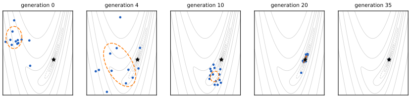
6.7.7 LLMs for DFO
p. 314 Large language models can propose candidate functions or programs from past evaluations (zero-shot or in context), or act as the mutation operator inside an evolutionary search (FunSearch). This is described qualitatively; it needs a language model and is not reproduced here.
S7.2 Dynamic programming (supplement)
Supp. pp. 70–71 Dynamic programming finds a global optimum when the optimal solution is built from optimal solutions of overlapping subproblems. The example is the Fibonacci recursion \(F_i=F_{i-1}+F_{i-2}\), \(F_0=F_1=1\) (7.75); the machine-learning uses are the forward–backward and Viterbi algorithms for HMMs, inference in graphical models and reinforcement learning.
Filling the gap 6.24: the naive recursion makes \(2F_n-1\) calls; memoisation and the bottom-up scheme are linear Supp. pp. 70–71, Algorithms 7.1–7.2
Derivation
Let \(T(n)\) be the number of calls made by the top-down recursion of Algorithm 7.1: \(T(0)=T(1)=1\) and \(T(n)=T(n-1)+T(n-2)+1\). Then \(U(n)=T(n)+1\) satisfies \(U(n)=U(n-1)+U(n-2)\) with \(U(0)=U(1)=2=2F_0=2F_1\), so \(U(n)=2F_n\) and \(T(n)=2F_n-1\) by induction. Since \(F_n\sim\varphi^{n+1}/\sqrt5\) (\(\varphi=(1+\sqrt5)/2\)), the cost is exponential. For \(n=5\): \(T=2\cdot8-1=15\) calls, with fib(2) evaluated three times, as in (7.76)–(7.79). Memoisation stores each value after its first computation (each \(F_i\), \(i\le n\), is computed once: \(O(n)\) additions) and the bottom-up loop of Algorithm 7.2 does the same without recursion overhead. The initialisation printed in Algorithm 7.2 ("\(F_1:=2\)") should be \(F_1:=1\) to match (7.75). The numbers \(T(n)=2F_n-1\) were confirmed by direct counting for \(n\le17\).
6.8 Optimal transport
pp. 314–322 This section (written by M. Cuturi) introduces optimal transport (OT) as the problem of moving one distribution onto another at least cost, starting from matchings and ending at the entropic regularisation that makes it computable at scale.
6.8.1 Warm-up: matching optimally two families of points
pp. 314–315 Given points \((\bm x_i)_{i\le n}\), \((\bm y_j)_{j\le n}\) and a cost \(C_{ij}=c(\bm x_i,\bm y_j)\), an optimal matching is a permutation \(\sigma\) minimising \(E(\sigma)=\sum_ic(\bm x_i,\bm y_{\sigma_i})\) (6.191). Enumeration costs \(n!\) but the Hungarian algorithm solves it in \(O(n^3)\).
6.8.2 From optimal matchings to Kantorovich and Monge formulations
pp. 316–317 To allow different numbers of points and split masses, give each point a weight, \(\sum_ia_i\delta_{\bm x_i}\) and \(\sum_jb_j\delta_{\bm y_j}\) with \(\sum a_i=\sum b_j\), and minimise over transport plans \(P\in U(a,b)=\{P\in\R_+^{n\times m}:P\bm1=a,P^\T\bm1=b\}\): \(\OT_C(a,b)=\min_{P\in U(a,b)}\langle P,C\rangle\) (6.192). For densities, the Monge problem seeks a map \(T\) with \(T_\sharp\mu=\nu\) (in smooth form \(q(T(\bm x))=p(\bm x)|J_T(\bm x)|\), (6.193)) minimising \(\int c(\bm x,T(\bm x))\mu(\mathrm d\bm x)\) (6.194); it is non-convex (a convex combination of two push-forward maps need not push \(\mu\) to \(\nu\)). The Kantorovich problem relaxes it to couplings \(\pi\in\Pi(\mu,\nu)\): \(\OT_c(\mu,\nu)=\inf_\pi\int c\,\mathrm d\pi\) (6.196), a linear program that always has the product coupling \(\mu\otimes\nu\) as a feasible point. With \(c=d^p\), \(W_p(\mu,\nu)=(\inf_\pi\int d^p\mathrm d\pi)^{1/p}\) is the Wasserstein distance (6.197).
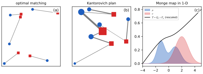
6.8.3 Solving optimal transport
pp. 318–322 Duality and cost concavity: the dual of (6.192) is \(\max\{\bm f^\T\bm a+\bm g^\T\bm b:\ f_i+g_j\le C_{ij}\}\) (6.198), and for measures \(\sup_{f\oplus g\le c}\int f\mathrm d\mu+\int g\,\mathrm d\nu\) (6.199). For a given \(f\) the best \(g\) is the \(c\)-transform \(\bar f(y)=\inf_x\{c(x,y)-f(x)\}\) (6.200), leading to the semi-dual \(\sup_{f\in\mathcal F_c}\int f\mathrm d\mu+\int\bar f\mathrm d\nu\) (6.203) over \(c\)-concave functions. Kantorovich–Rubinstein: for \(c=d\), \(W_1(\mu,\nu)=\sup_{f\ 1\text{-Lipschitz}}\int f\,\mathrm d(\mu-\nu)\) (6.204). Brenier: for \(c=\frac12\|x-y\|^2\) and \(\mu\) with a density the optimal Monge map exists and is the gradient of a convex function (6.205–6.208). Closed forms: in one dimension \(\OT_c(\mu,\nu)=\int_0^1c(Q_\mu(u),Q_\nu(u))\mathrm du\) (6.209) with Monge map \(Q_\nu\circ F_\mu\); for Gaussians \(W_2^2=\|\bm m_1-\bm m_2\|^2+\mathcal B^2(\Sigma_1,\Sigma_2)\) with the Bures term \(\mathcal B^2=\Tr(\Sigma_1+\Sigma_2-2(\Sigma_1^{1/2}\Sigma_2\Sigma_1^{1/2})^{1/2})\) (6.210–6.211) and the map \(T(\bm x)=A(\bm x-\bm m_1)+\bm m_2\) (6.212). Entropic regularisation (Cuturi, 2013): \(W_{c,\gamma}=\inf_\pi\int c\,\mathrm d\pi+\gamma\KL(\pi\|\mu\otimes\nu)\) (6.213), solved by the Sinkhorn iterations (6.217).
Filling the gap 6.25: weak duality, the \(c\)-transform identities (the correct form of (6.202)), and Kantorovich–Rubinstein duality pp. 318–319, (6.198)–(6.204)
Derivation
Weak duality. If \(f_i+g_j\le C_{ij}\) for all \(i,j\) and \(P\in U(a,b)\) then \(\langle P,C\rangle\ge\sum_{ij}P_{ij}(f_i+g_j)=\bm f^\T\bm a+\bm g^\T\bm b\). Both problems are linear programs, so strong duality (equality of the optima) holds when they are feasible and bounded, which they are (\(ab^\T\in U(a,b)\) and \(C\) is finite). The transport polytope is compact, so a minimiser exists. For \(n=m\) and \(a=b=\bm1/n\), the vertices of \(U\) are the permutation matrices divided by \(n\) (Birkhoff–von Neumann), so the optimal value is attained at a matching: the Kantorovich problem generalises (6.191) (checked: LP optimum = Hungarian optimum). The numerical dual solution also equals the primal optimum to \(10^{-9}\).
\(c\)-transforms. For \(f:\mathcal X\to\R\) let \(\bar f(y)=\inf_x\{c(x,y)-f(x)\}\) and, for \(g:\mathcal Y\to\R\), \(\tilde g(x)=\inf_y\{c(x,y)-g(y)\}\) (6.201). (i) \(f\le\tilde{\bar f}\): by definition of \(\bar f\), \(\bar f(y)\le c(x,y)-f(x)\) for all \(x,y\), i.e. \(f(x)\le c(x,y)-\bar f(y)\) for all \(y\), so \(f(x)\le\inf_y\{c(x,y)-\bar f(y)\}\). (ii) The transform reverses order: \(f\le h\Rightarrow\bar f\ge\bar h\). Apply (ii) to (i): \(\bar f\ge\bar{\tilde{\bar f}}\). Apply (i) (with roles swapped) to \(g=\bar f\): \(\bar f\le\bar{\tilde{\bar f}}\). Hence \(\bar f=\bar{\tilde{\bar f}}\): applying the transforms three times is the same as once. The printed (6.202), "\(\tilde{\bar f}=f\)", is therefore true only for \(c\)-concave \(f\), the functions of the form \(\tilde g\) (for them (i) is an equality, which is how \(\mathcal F_c\) is defined). Restricting the dual to such pairs \((f,\bar f)\) removes the free variable \(g\) without loss: this is the semi-dual (6.203). (Checked on random potentials on a grid.)
Kantorovich–Rubinstein. Take \(c=d\), a metric, and \(f=\tilde g\), i.e. \(f(x)=\inf_y\{d(x,y)-g(y)\}\). As an infimum of 1-Lipschitz functions of \(x\), \(f\) is 1-Lipschitz. For \(1\)-Lipschitz \(f\): \(f(x)\le f(y)+d(x,y)\) so \(d(x,y)-f(x)\ge-f(y)\) and \(\bar f(y)\ge-f(y)\); taking \(x=y\) gives \(\bar f(y)\le-f(y)\); hence \(\bar f=-f\). Conversely every 1-Lipschitz function is \(d\)-concave (the same inequality shows \(f=\tilde{\bar f}\) with \(\bar f=-f\)). Therefore the semi-dual (6.203) reads \(\sup_{f\ 1\text{-Lip}}\int f\mathrm d\mu-\int f\mathrm d\nu\), which is (6.204). (Checked by solving this Lipschitz-constrained LP on a 24-point support: equals the primal \(W_1\) to \(10^{-8}\).)
Filling the gap 6.26: the one-dimensional and Gaussian closed forms, and why a gradient of a convex function is an optimal map (Brenier) pp. 319–321, (6.205)–(6.212)
Derivation
One dimension. Let \(h\) be convex, \(x<x'\) and \(y<y'\). Put \(a=x-y'\), \(b=x-y\), \(c=x'-y'\), \(d=x'-y\); then \(a\le b,c\le d\) and \(a+d=b+c\), so by convexity \(h(b)+h(c)\le h(a)+h(d)\), i.e. \(h(x-y)+h(x'-y')\le h(x-y')+h(x'-y)\): matching in the same order is never worse than crossing. Any non-monotone matching can be uncrossed repeatedly without raising the cost, so the sorted matching is optimal; for weighted points the same exchange argument applies to portions of mass, and the optimal plan is the monotone (north-west corner) coupling; in the limit, the quantile coupling (6.209), \(T=Q_\nu\circ F_\mu\). For \(c=|x-y|\), \(\int_0^1|Q_\mu-Q_\nu|\mathrm du=\int|F_\mu-F_\nu|\mathrm dx\) (the same area, integrated along the other axis): \(W_1\) is the area between the cdfs, not the Kolmogorov–Smirnov statistic \(\sup|F_\mu-F_\nu|\) as the book states. (Checked: LP = sorted matching to \(10^{-9}\); LP = north-west corner for unequal weights; \(W_1\) = cdf area.)
Optimality of \(\nabla u\) for convex \(u\). Let \(u\) be convex with \(T=\nabla u\) and \(T_\sharp\mu=\nu\). Fenchel–Young (Gap 6.17) gives \(u(\bm x)+u^\ast(\bm y)\ge\langle\bm x,\bm y\rangle\), with equality iff \(\bm y=\nabla u(\bm x)\). For any coupling \(\pi\in\Pi(\mu,\nu)\), \(\int\langle\bm x,\bm y\rangle\mathrm d\pi\le\int u\,\mathrm d\mu+\int u^\ast\mathrm d\nu\), with equality for \(\pi=(\mathrm{Id},T)_\sharp\mu\). Since the marginals are fixed, \(\int\frac12\|\bm x-\bm y\|^2\mathrm d\pi=\frac12\int\|\bm x\|^2\mathrm d\mu+\frac12\int\|\bm y\|^2\mathrm d\nu-\int\langle\bm x,\bm y\rangle\mathrm d\pi\), so the coupling induced by \(T\) is optimal. The converse and uniqueness (the optimal map exists and is a gradient of a convex function when \(\mu\) has a density) is Brenier's theorem (1991): the book's sketch uses complementary slackness, \(f^\ast(\bm x_0)+\bar f^\ast(\bm y_0)=c(\bm x_0,\bm y_0)\) on the support, which for the quadratic cost forces \(\bm y_0=\bm x_0-\nabla f^\ast(\bm x_0)=\nabla(\frac12\|\cdot\|^2-f^\ast)(\bm x_0)\), and \(\frac12\|\cdot\|^2-f^\ast\) is convex because \(f^\ast\) is \(c\)-concave.
Gaussians. Let \(M=\Sigma_1^{1/2}\Sigma_2\Sigma_1^{1/2}\) and \(A=\Sigma_1^{-1/2}M^{1/2}\Sigma_1^{-1/2}\), symmetric positive definite. Then \(A\Sigma_1A=\Sigma_1^{-1/2}M^{1/2}M^{1/2}\Sigma_1^{-1/2}=\Sigma_2\), so \(T(\bm x)=A(\bm x-\bm m_1)+\bm m_2\) pushes \(\N(\bm m_1,\Sigma_1)\) to \(\N(\bm m_2,\Sigma_2)\) (an affine image of a Gaussian), and \(T=\nabla u\) with \(u(\bm x)=\frac12(\bm x-\bm m_1)^\T A(\bm x-\bm m_1)+\bm m_2^\T\bm x\) convex, hence optimal by the previous paragraph. Its cost is \(\E\|\bm X-T(\bm X)\|^2=\|\bm m_1-\bm m_2\|^2+\Tr((I-A)\Sigma_1(I-A))=\|\bm m_1-\bm m_2\|^2+\Tr\Sigma_1+\Tr\Sigma_2-2\Tr(A\Sigma_1)\) and \(A\Sigma_1=\Sigma_1^{-1/2}M^{1/2}\Sigma_1^{1/2}\) has trace \(\Tr M^{1/2}\) (cyclicity): (6.210)–(6.211). In one dimension this is \((m_1-m_2)^2+(s_1-s_2)^2\) (checked). Monte Carlo with \(6\times10^4\) draws reproduces the Bures value to \(0.05\), and a random re-pairing of the same samples costs more.
6.8.3.6 Obtaining smoothness using entropic regularization
pp. 321–322 The exact LP costs \(O(n^3\log n)\) and its sample complexity in dimension \(q\) is \(n^{-1/q}\) (so solving it exactly on samples overfits in high dimension). Regularising with the KL divergence to the product measure makes the problem strongly convex and solvable by alternating rescalings.
Filling the gap 6.27: the Sinkhorn form of the plan, the KL identity, the dual, and why the iteration is block-coordinate ascent pp. 321–322, (6.213)–(6.217)
Derivation
The identity. For \(P\in U(a,b)\), \(\sum_{ij}P_{ij}\log(a_ib_j)=\sum_ia_i\log a_i+\sum_jb_j\log b_j=-H(a)-H(b)\) with the Shannon entropy \(H(p)=-\sum p\log p\), hence \(\KL(P\|ab^\T)=\sum P_{ij}\log P_{ij}+H(a)+H(b)=-H(P)+H(a)+H(b)\). So (6.214) is \(\langle P,C\rangle+\gamma\KL(P\|ab^\T)\).
Form of the solution. The objective is \(\gamma\)-strongly convex on the compact polytope \(U(a,b)\), so there is a unique minimiser; as \(x\log x\) has infinite slope at 0, it has all entries positive. With multipliers \(\bm f,\bm g\) for the marginal constraints, stationarity of \(\langle P,C\rangle+\gamma\sum P_{ij}\log P_{ij}-\sum_if_i(\sum_jP_{ij}-a_i)-\sum_jg_j(\sum_iP_{ij}-b_j)\) in \(P_{ij}\) gives \(C_{ij}+\gamma(\log P_{ij}+1)-f_i-g_j=0\), i.e. \(P_{ij}=e^{(f_i+g_j-C_{ij})/\gamma-1}=u_iK_{ij}v_j\) with \(K=e^{-C/\gamma}\), \(u=e^{f/\gamma}\), \(v=e^{g/\gamma}\) (the \(-1\) absorbed into the potentials): (6.216).
Dual. Substituting this \(P\) (which has \(\sum P=1\) at the optimum) into the Lagrangian gives the dual \(\bm f^\T\bm a+\bm g^\T\bm b-\gamma\sum_{ij}e^{(f_i+g_j-C_{ij})/\gamma}+\mathrm{const}\), i.e. (6.215) \(\bm f^\T\bm a+\bm g^\T\bm b-\gamma(e^{\bm f/\gamma})^\T Ke^{\bm g/\gamma}+\gamma(1+H(a)+H(b))\). At the optimum \(\sum P=1\), so the middle term is \(-\gamma\), and the primal value (6.214) \(=\langle P,C\rangle-\gamma H(P)+\gamma(H(a)+H(b))\); since \(\log P_{ij}=(f_i+g_j-C_{ij})/\gamma\), \(-\gamma H(P)=\gamma\sum P\log P=\bm f^\T\bm a+\bm g^\T\bm b-\langle P,C\rangle\) and the two values coincide: \(\bm f^\T\bm a+\bm g^\T\bm b+\gamma(H(a)+H(b))\), equal to (6.215) (checked numerically to \(10^{-9}\)).
Sinkhorn as coordinate ascent. The dual is concave. Setting the derivative in \(f_i\) to zero, \(a_i-e^{f_i/\gamma}\sum_jK_{ij}e^{g_j/\gamma}=0\), gives \(f_i=\gamma\log a_i-\gamma\log\sum_jK_{ij}e^{g_j/\gamma}\), the first line of (6.217); the same in \(g_j\) gives the second. Each update therefore exactly maximises the dual over one block, so the dual increases monotonically, and after the \(g\)-update the column marginals are exact (the row marginals after the \(f\)-update). A fixed point has both marginals correct and the form (6.216), hence satisfies the KKT conditions and is the solution. Convergence of the iterates follows from strict concavity modulo the shift \((f+t,g-t)\) and boundedness by the primal value; the linear rate, with a factor below 1 depending on \(\max_{ij}C_{ij}/\gamma\) through the Hilbert projective metric (Franklin and Lorenz, 1989), degrades as \(\gamma\to0\). In the demonstration on the iris petal lengths, the marginal error falls below \(10^{-10}\) after 24, 113 and 821 iterations for \(\gamma=0.5,0.1,0.02\).
Limits. As \(\gamma\to\infty\) the KL term dominates and \(P\to ab^\T\) (checked); as \(\gamma\to0\), \(P_\gamma\) converges to the optimal plan of maximal entropy and \(\langle P_\gamma,C\rangle\downarrow\OT_C(a,b)\) (the cost decreases monotonically to the exact value in the numerical runs). The bias \(\langle P_\gamma,C\rangle-\OT\) shrinks with \(\gamma\) while the cost of the algorithm grows (Figure x6.d).
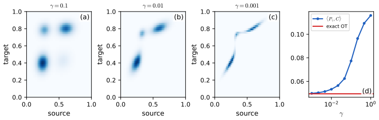
6.9 Submodular optimization
pp. 322–342 This section (written by J. Bilmes) introduces set functions \(f:2^V\to\R\) with a diminishing-returns property. Like convexity, submodularity makes optimisation tractable, but a submodular function can both be minimised exactly in polynomial time and be maximised approximately; the two problems model different needs (homogeneity against diversity).
6.9.1 Intuition, examples, and background
pp. 322–325 Notation: \(f(v\given X)=f(X+v)-f(X)\) (the gain of \(v\) in context \(X\)), \(f(X\given Y)=f(X\cup Y)-f(Y)\). In the coffee, lemon, milk and tea example, \(f(\emptyset)=0\) and the valuations (Figure 6.19) show substitutes (coffee and tea: \(f(c,t)<f(c)+f(t)\), subadditive), complements (milk and coffee: superadditive), independent items (lemon and milk: modular), and context-dependent relations: given tea, lemon and milk are substitutes (\(f(l\given m,t)<f(l\given t)\)) but given milk, tea and lemon are complements (\(f(t\given l,m)>f(t\given m)\)). The function is therefore neither submodular nor supermodular. Typical machine-learning objectives are one or the other everywhere.
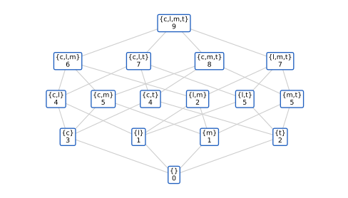
6.9.2 Submodular basic definitions
pp. 325–326 Definition 6.9.1: \(f\) is submodular if \(f(X)+f(Y)\ge f(X\cup Y)+f(X\cap Y)\) for all \(X,Y\subseteq V\) (6.218). Definition 6.9.2 (diminishing returns): \(f(X+v)-f(X)\ge f(Y+v)-f(Y)\) whenever \(X\subseteq Y\), \(v\notin Y\) (6.219). \(f\) is supermodular if \(-f\) is submodular and modular if both, i.e. \(m(A)=c+\sum_{v\in A}m_v\); monotone if \(f(A)\le f(B)\) for \(A\subseteq B\); a normalised monotone submodular function is a polymatroid function. Shannon entropy as a function of subsets of random variables is a polymatroid function (not every polymatroid function is entropic). Nonnegative combinations of submodular functions are submodular.
Filling the gap 6.28: (6.218) is equivalent to (6.219), the standard examples are submodular, and curvature zero means modular pp. 325–329, (6.218)–(6.222)
Derivation
(6.218) \(\Rightarrow\) (6.219). Given \(X\subseteq Y\), \(v\notin Y\), apply (6.218) to \(A=X+v\) and \(B=Y\): \(A\cup B=Y+v\), \(A\cap B=X\), so \(f(X+v)+f(Y)\ge f(Y+v)+f(X)\), which rearranges to (6.219).
(6.219) \(\Rightarrow\) (6.218). Let \(Y\setminus X=\{y_1,\dots,y_k\}\) and \(Y_i=\{y_1,..,y_{i-1}\}\). Telescoping, \(f(X\cup Y)-f(X)=\sum_if(y_i\given X\cup Y_i)\le\sum_if(y_i\given(X\cap Y)\cup Y_i)=f(Y)-f(X\cap Y)\), using (6.219) with \(X\cap Y\cup Y_i\subseteq X\cup Y_i\). This is (6.218).
Closure and examples. Nonnegative combinations: (6.218) is linear in \(f\). Concave of modular: \(f(A)=\varphi(m(A))\), \(m\ge0\), \(\varphi\) concave: the gain \(\varphi(m(A)+m_v)-\varphi(m(A))\) decreases in \(m(A)\), hence along inclusions. Facility location \(f(A)=\sum_{v\in V}\max_{a\in A}s(a,v)\), \(s\ge0\): for each \(v\) the term \(\max_{a\in A}s_{a}\) has gain \((s_{a'}-\max_{a\in A}s_a)_+\), decreasing in \(A\); it is monotone. It is feature-based: if \(0=x_0\le x_1\le\dots\le x_n\) and \(y_i=x_i-x_{i-1}\), then \(\max_{a\in A}x_a=\sum_iy_i\min(|A\cap\{i,\dots,n\}|,1)\), because if the largest index in \(A\) is \(k\), the terms \(i\le k\) equal \(y_i\) and the others vanish, summing to \(x_k\) (checked on all subsets). Set cover \(|\bigcup_{v\in A}U_v|=\sum_u\min(1,m_u(A))\) and probabilistic coverage \(\sum_u\omega_u(1-\prod_{v\in A}(1-p_{uv}))=\sum_u\omega_u(1-e^{-m_u(A)})\) with \(m_u(v)=-\log(1-p_{uv})\) are concave-of-modular sums. Graph cut \(f(X)=\sum_{i\in X,j\notin X}w_{ij}\): split nodes into \(A=X\cap Y\), \(B=X\setminus Y\), \(C=Y\setminus X\), \(D=V\setminus(X\cup Y)\); then \(f(X)+f(Y)-f(X\cup Y)-f(X\cap Y)=2w(B,C)\ge0\), so cut is submodular (not monotone; it is the sum (6.222) of non-normalised feature-based functions). Log-determinant \(f(X)=\log\det M_X\), \(M\succ0\): the gain \(f(v\given X)=\log(M_{vv}-M_{vX}M_X^{-1}M_{Xv})\) is the log of the conditional variance of \(Y_v\) given \(Y_X\) for \(Y\sim\N(0,M)\); the conditional variance is the minimum of \(\E(Y_v-\bm\beta^\T Y_X)^2\) over \(\bm\beta\), which cannot increase when \(X\) grows. So the gains decrease and \(f\) is submodular but not monotone (a gain can be negative). Shannon entropy: \(H(X_v\given X_A)\) decreases as the conditioning set grows (conditioning reduces entropy). All of these were checked by brute force over all pairs of subsets (violation \(\le10^{-9}\)), as were the equivalence of (6.218) and (6.219) on 300 random set functions and the example function of Figure 6.19 (neither submodular nor supermodular).
Curvature. With \(\kappa=1-\min_vf(v\given V-v)/f(v)\), \(\kappa=0\) iff \(f(v\given V-v)=f(v)\) for every \(v\); by diminishing returns \(f(v)\ge f(v\given X)\ge f(v\given V-v)\) for all \(X\not\ni v\), so then every gain equals \(f(v)\) and \(f(A)=\sum_{v\in A}f(v)\) is modular. Conversely a modular function has all gains equal to \(f(v)\).
6.9.3 Example submodular functions
pp. 327–329 \(\sqrt{|A|}\) and more generally \(\varphi(m(A))\) with \(\varphi\) concave; feature-based functions \(\sum_u\varphi_u(m_u(A))+m_\pm(A)\) (a sum over features of concave functions of non-negative modular scores, plus an arbitrary modular term); facility location, called the \(k\)-means of submodular functions because it needs only an affinity matrix; set cover, vertex cover, edge cover and probabilistic coverage; graph cut and the cooperative cut; and deep submodular functions, nested compositions of concave functions that strictly generalise feature-based ones. Proofs for the main examples are in Gap 6.28.
6.9.4 Submodular optimization
pp. 329–333 Maximisation (diversity, coverage): \(\max_{A\in\mathcal C}f(A)\) for a constraint set \(\mathcal C\). Cardinality-constrained maximisation is NP-complete but the greedy algorithm \(X_{i+1}=X_i\cup\{\argmax_{v\notin X_i}f(X_i\cup v)\}\) (6.223) is within \(1-1/e\approx0.63\) of the optimum for monotone submodular \(f\) (Nemhauser, Wolsey and Fisher, 1978), and no polynomial algorithm does better unless P = NP (Feige, 1998). With total curvature \(\kappa\) the guarantee improves to \(\frac1\kappa(1-e^{-\kappa})\) (Conforti and Cornuéjols, 1984), equal to 1 for modular \(f\). Knapsack constraints need a cost-scaled greedy, a matroid constraint (for example at most \(\ell_i\) from each block of a partition, (6.224)) gives a \(\frac12\) guarantee for greedy. Minimisation (homogeneity, coherence): unconstrained minimisation of a submodular function is solvable in polynomial time (Grötschel, Lovász and Schrijver, 1981; combinatorial algorithms by Iwata, Fleischer, Fujishige and by Schrijver around 2000; practical methods minimise the 2-norm over the base polytope), by way of the convex Lovász extension, which is why submodular functions are called a discrete form of convexity.
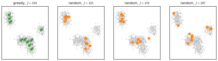
Filling the gap 6.29: the greedy algorithm achieves \(1-(1-1/k)^k\ge1-1/e\) for monotone submodular maximisation pp. 330–331, (6.223)
Derivation
Theorem (Nemhauser, Wolsey and Fisher, 1978). Let \(f\ge0\) be monotone submodular with \(f(\emptyset)=0\), let \(O\) maximise \(f\) among sets of size \(\le k\), and let \(X_i\) be the greedy set after \(i\) steps. Then \(f(X_k)\ge(1-(1-\tfrac1k)^k)f(O)\ge(1-e^{-1})f(O)\).
Proof. Fix \(i<k\). Monotonicity gives \(f(O)\le f(O\cup X_i)\). List \(O\setminus X_i=\{o_1,\dots,o_r\}\), \(r\le k\); telescoping and diminishing returns (6.219) give \(f(O\cup X_i)-f(X_i)=\sum_jf(o_j\given X_i\cup\{o_1..o_{j-1}\})\le\sum_jf(o_j\given X_i)\le k\max_{v}f(v\given X_i)\). The greedy step picks the maximiser, \(f(X_{i+1})-f(X_i)=\max_vf(v\given X_i)\). Hence \(f(O)-f(X_i)\le k\,(f(X_{i+1})-f(X_i))\). With \(\delta_i=f(O)-f(X_i)\) this says \(\delta_{i+1}\le(1-\tfrac1k)\delta_i\), so \(\delta_k\le(1-\tfrac1k)^k\delta_0\le e^{-1}f(O)\) (as \(1-x\le e^{-x}\)), i.e. \(f(X_k)\ge(1-e^{-1})f(O)\). \(\square\)
The proof uses monotonicity and (6.219) only, whatever \(f\) is. Numerically, on 300 random coverage instances with ground set 9 and \(k\in\{2,3,4\}\), the worst ratio of greedy to the brute-force optimum was above \(1-1/e=0.632\) (typical ratios are far higher), and greedy is exactly optimal for a modular function.
For non-monotone submodular functions (graph cut, log-determinant) the first step \(f(O)\le f(O\cup X_i)\) fails, so this proof gives no guarantee; maximising such functions needs other algorithms (the book points to randomised double greedy and constrained variants), and the constraint set \(\mathcal C\) of Section 6.9.4.2, for example the partition matroid (6.224), changes the guarantee to \(\tfrac12\) for greedy.
6.9.5–6.9.12 Applications and conclusions
pp. 333–342 The remaining subsections survey uses of submodularity and are summarised here without derivations; all of them reduce to maximising or minimising a submodular function with the algorithms above. Summarisation, coresets, distillation and subset selection (6.9.6): choose \(X\) maximising an information function \(f(X)\) so that the residual information \(f(V\setminus X\given X)=f(V)-f(X)\) is small; the submodular function can be handcrafted (facility location from a similarity matrix), learned as a mixture \(\sum_i\alpha_if_i\) (a regression for the coefficients), or chosen so that the objective is provably a coreset bound. Combinatorial information functions (6.9.7): for any polymatroid \(f\), the combinatorial conditional mutual information \(I_f(A;B\given C)=f(A+C)+f(B+C)-f(C)-f(A+B+C)\), equal to the usual mutual information when \(f\) is entropy. Clustering and partitioning (6.9.8): recursive minimisation of the symmetric submodular function \(I_f(A;V\setminus A)\) (Queyranne's algorithm), or facility location as \(k\)-medoids. Active and semi-supervised learning (6.9.9): a batch \(A_t\in\argmax\{m_t(A)+f_t(A)\}\) combining a modular uncertainty score \(m_t\) with a submodular diversity term \(f_t\). Probabilistic modelling (6.9.10): the MAP assignment of a model with energy \(E(\bm x)=f(V(\bm x))\), \(f\) submodular, is a submodular minimisation (graph cuts for MRFs); \(\log\det\) gives determinantal point processes, log-submodular models that favour diverse sets. Structured norms and losses (6.9.11): penalising \(f(\mathrm{supp}(\bm x))\) for submodular \(f\), whose convex envelope is the Lovász-extension norm, generalises the \(\ell_0\), \(\ell_1\) and group-lasso penalties.
6.10 Exercises
The chapter has no end-of-chapter exercises in the book. Three short practice problems follow, with complete solutions (hidden).
Exercise 6.1 (bound optimisation against Newton). A one-feature logistic regression without bias has data \(x=(-2,-1,1,2)\), labels \(y=(0,1,0,1)\). (a) Show that \(H(w)\succeq-\tfrac14\sum_nx_n^2\) for all \(w\). (b) Starting from \(w_0=0\), compute the first two iterates of the bound-optimisation iteration (6.134) and of Newton's method, and the limit. (c) Explain why the first iterates coincide.
Solution
(a) \(H(w)=-\sum_n\mu_n(1-\mu_n)x_n^2\) and \(\mu_n(1-\mu_n)\le\tfrac14\), so \(H(w)\ge-\tfrac14\sum x_n^2=-\tfrac{10}4=-2.5\). (b) \(g(w)=\sum_n(y_n-\mu_n)x_n\). At \(w_0=0\), \(\mu_n=\tfrac12\): \(g=(-\tfrac12)(-2)+\tfrac12(-1)+(-\tfrac12)(1)+\tfrac12(2)=1\). The MM step is \(w_1=w_0+4g/\sum x^2=0.4\). At \(w=0\) the Newton Hessian is \(-\tfrac14\sum x^2=-2.5\), the same, so Newton also gives \(w_1=0.4\). Second iterates (computed with the companion code): MM \(0.41709\), Newton \(0.41949\); the iterates continue MM \(0.41928,0.41957,0.41961,0.419617\) and Newton \(0.419618\) (converged after 3 steps); the MLE is \(\hat w=0.419618\) and \(\ell(\hat w)=-2.56781\). (c) The bound \(B=-\tfrac14X^\T X\) is exact where \(\mu_n=\tfrac12\) for all \(n\), i.e. at \(w=0\); afterwards the true curvature \(\sum\mu_n(1-\mu_n)x_n^2\) falls below \(2.5\), the surrogate is looser, and MM converges linearly (rate \(\approx1-H(\hat w)/B\), about \(0.13\) here, so each step cuts the error roughly 7-fold) against Newton's quadratic convergence. Both increase the log-likelihood monotonically. (Using the printed sign \(w-4(X^\T X)^{-1}g\) would send \(w_1\) to \(-0.4\), a decrease of \(\ell\).)
Exercise 6.2 (natural gradient for a Gaussian fit). Fit \(\N(\mu,\sigma^2)\) to data with mean \(\bar x\) and variance \(s^2\) by minimising the mean NLL \(L(\mu,\sigma)=\log\sigma+\tfrac12\log2\pi+\frac{s^2+(\bar x-\mu)^2}{2\sigma^2}\). (a) Find the gradient and the Fisher matrix in \((\mu,\sigma)\). (b) Write the natural-gradient update. (c) With \(\eta=1\), show that \(\mu\) reaches \(\bar x\) in one step and that \(\sigma\) then follows the Babylonian square-root iteration to \(s\).
Solution
(a) \(\partial_\mu L=(\mu-\bar x)/\sigma^2\), \(\partial_\sigma L=1/\sigma-(s^2+(\bar x-\mu)^2)/\sigma^3\). The score of \(\N(\mu,\sigma^2)\) is \(((y-\mu)/\sigma^2,\,-1/\sigma+(y-\mu)^2/\sigma^3)\) with covariance \(F=\diag(1/\sigma^2,2/\sigma^2)\) (using \(\E(y-\mu)^2=\sigma^2\), \(\E(y-\mu)^4=3\sigma^4\)). (b) \(F^{-1}\bm g=(\mu-\bar x,\ \tfrac12(\sigma-(s^2+(\bar x-\mu)^2)/\sigma))\), so \(\mu_{t+1}=\mu_t-\eta(\mu_t-\bar x)\) and \(\sigma_{t+1}=\sigma_t-\frac\eta2\big(\sigma_t-\frac{s^2+(\mu_t-\bar x)^2}{\sigma_t}\big)\). (c) With \(\eta=1\), \(\mu_1=\bar x\) and \(\sigma_{t+1}=\tfrac12\big(\sigma_t+\frac{s^2+(\mu_t-\bar x)^2}{\sigma_t}\big)\); from \(t=1\) on, \(\sigma_{t+1}=\tfrac12(\sigma_t+s^2/\sigma_t)\), Heron's iteration for \(\sqrt{s^2}\), which converges quadratically to \(s\) from any \(\sigma_1>0\). On the iris versicolor sepal lengths (\(\bar x=5.936\), \(s^2=0.2611\)) started at \((4.5,0.3)\), the loss gap after 30 steps is \(1.2\times10^{-15}\) with \(\eta=0.5\) in \((\mu,\sigma)\) (and \(4.5\times10^{-5}\) in \((\mu,\log\sigma)\)), against \(2.28\) for steepest descent with \(\eta=0.1\) in \((\mu,\sigma)\), as in the demonstration.
Exercise 6.3 (entropic transport in closed form). Let \(a=b=(\tfrac12,\tfrac12)\) and \(C=\begin{pmatrix}0&1\\1&0\end{pmatrix}\). Find the entropic plan \(P_\gamma\) and its cost, and the exact optimal plan.
Solution
Every plan in \(U(a,b)\) is \(P=\begin{pmatrix}p&\frac12-p\\\frac12-p&p\end{pmatrix}\), \(0\le p\le\frac12\), with cost \(\langle P,C\rangle=1-2p\). The regularised objective is \(1-2p+\gamma[2p\log p+2(\tfrac12-p)\log(\tfrac12-p)]+\const\) (the KL to \(ab^\T\) differs by a constant). Setting the derivative to zero: \(-2+2\gamma\log\frac p{1/2-p}=0\), so \(\frac p{1/2-p}=e^{1/\gamma}\) and \(p=\tfrac12\sigma(1/\gamma)\) with \(\sigma\) the sigmoid. Hence \(P_\gamma=\tfrac12\begin{pmatrix}\sigma(1/\gamma)&\sigma(-1/\gamma)\\\sigma(-1/\gamma)&\sigma(1/\gamma)\end{pmatrix}\) and \(\langle P_\gamma,C\rangle=\sigma(-1/\gamma)=1/(1+e^{1/\gamma})\). This has the form \(\mathrm{diag}(u)K\mathrm{diag}(v)\), \(K=\begin{pmatrix}1&e^{-1/\gamma}\\e^{-1/\gamma}&1\end{pmatrix}\), as (6.216) requires. As \(\gamma\to0\), \(P_\gamma\to\tfrac12I\) (the exact optimal plan, cost 0) with bias \(\approx e^{-1/\gamma}\); as \(\gamma\to\infty\), \(P_\gamma\to\tfrac14\bm1\bm1^\T=ab^\T\) with cost \(\tfrac12\). (Sinkhorn's iteration reproduces these entries to rounding.)
Demonstrations
Notes on the book
Slips and sharpenings found while proving the claims
- (6.44), Robbins–Monro conditions. The printed condition (\(\sum\eta_t^2/\sum\eta_t\to0\)) is garbled; the conditions are \(\sum_t\eta_t=\infty\) and \(\sum_t\eta_t^2<\infty\) (and \(\eta_t\to0\) is enough for strongly convex problems) (gap 6.2).
- (6.61), Rao–Blackwellisation. The second term should carry the weight \(q_\theta(S_2)=\Pr(\bm z\in S_2)\) in front of the conditional expectation (gap 6.3).
- (6.87)–(6.90), trust region. With the penalty written as \(\eta\bm\delta^\T F\bm\delta\), the minimiser is \(-F^{-1}\bm g/(2\eta)\); the printed \(\bm\delta=-\eta F^{-1}\bm g\) corresponds to the penalty \(\bm\delta^\T F\bm\delta/(2\eta)\) (gap 6.9).
- (6.132), (6.125). The Hessian bound should be \(\succeq\) (not \(\succ\)): equality \(p=\frac12\) is attained (gap 6.13).
- (6.135), sign. For \(\bm g=X^\T(\bm y-\bm\mu)\) (the log-likelihood gradient) the update is \(\bm w+4(X^\T X)^{-1}\bm g\); the printed minus sign decreases the likelihood (gap 6.13, Exercise 6.1).
- (6.168). The expected complete-data log-likelihood also contains \(-\frac N2\log\sigma^2\); it matters as soon as \(\sigma^2\) is updated (gap 6.16). In (6.169), \(\delta_n\) should read \((y_n-\bm w^\T\bm x_n)^2/\sigma^2\).
- (6.192) and (6.214), indices. In (6.192) the constraints are written \(P\bm1_n=a\), \(P^\T\bm1_m=b\) for \(P\in\R^{n\times m}\); they should read \(P\bm1_m=a\), \(P^\T\bm1_n=b\), as in (6.214). (6.213) integrates \(d(x,y)^p\) where the cost \(c\) is meant.
- (6.202), \(c\)-transforms. The identity holds for \(c\)-concave \(f\) only; for general \(f\) the true statement is that three successive transforms equal one (gap 6.25).
- Section 6.8.3.4, \(W_1\) in one dimension. The text calls \(\OT_c\) for \(c=|x-y|\) "the Kolmogorov–Smirnov statistic"; it is the area between the two cdfs, whereas the KS statistic is their maximum distance (gap 6.26).
- (6.214)–(6.215), entropy convention. The constants \(\gamma(H(a)+H(b))\) and \(\gamma(1+\cdots)\) make the primal equal to \(\langle P,C\rangle+\gamma\KL(P\|ab^\T)\) and match the dual exactly when \(H\) is the Shannon entropy \(-\sum p\log p\) (gap 6.27).
- (7.24) and (7.25). The quadratic term in (7.24) is \(\frac1{2}(z-x)^2\) (printed "\(1\) over \(z\)"), and the cases of (7.25) are \(x-\lambda\) for \(x\ge\lambda\), \(0\) for \(|x|\le\lambda\), \(x+\lambda\) for \(x\le-\lambda\) (gap 6.18).
- (7.72), robust PCA. \(A/N\) should be \(A/J\), with \(J\) the number of blocks, as in (7.73) (gap 6.20).
- (7.87) and (7.108). In (7.87) the derivative of \(\lambda x-f(x)\) is \(\lambda-f'(x)=\lambda+e^{-x}\); in (7.108) the conjugate is \(-\lambda(\xi)\xi^2-f(\xi)\), consistent with (7.109) (gap 6.17).
- Algorithm 7.2, initialisation. \(F_1:=2\) should be \(F_1:=1\) to match (7.75) (gap 6.24).
References
- Murphy, K. P. (2023). Probabilistic Machine Learning: Advanced Topics. MIT Press, Cambridge, MA. Chapter 6 and online supplement Chapter 7. probml.github.io/pml-book/book2.html.
- Amari, S. (1998). Natural gradient works efficiently in learning. Neural Computation, 10(2), 251–276.
- Beck, A. and Teboulle, M. (2009). A fast iterative shrinkage-thresholding algorithm for linear inverse problems. SIAM Journal on Imaging Sciences, 2(1), 183–202.
- Bergstra, J. and Bengio, Y. (2012). Random search for hyper-parameter optimization. Journal of Machine Learning Research, 13, 281–305.
- Böhning, D. (1992). Multinomial logistic regression algorithm. Annals of the Institute of Statistical Mathematics, 44(1), 197–200.
- Boyd, S., Parikh, N., Chu, E., Peleato, B. and Eckstein, J. (2011). Distributed optimization and statistical learning via the alternating direction method of multipliers. Foundations and Trends in Machine Learning, 3(1), 1–122.
- Brenier, Y. (1991). Polar factorization and monotone rearrangement of vector-valued functions. Communications on Pure and Applied Mathematics, 44(4), 375–417.
- Conforti, M. and Cornuéjols, G. (1984). Submodular set functions, matroids and the greedy algorithm. Discrete Applied Mathematics, 7(3), 251–274.
- Cuturi, M. (2013). Sinkhorn distances: lightspeed computation of optimal transport. Advances in Neural Information Processing Systems, 26.
- Dempster, A. P., Laird, N. M. and Rubin, D. B. (1977). Maximum likelihood from incomplete data via the EM algorithm. Journal of the Royal Statistical Society B, 39(1), 1–38.
- Franklin, J. and Lorenz, J. (1989). On the scaling of multidimensional matrices. Linear Algebra and its Applications, 114/115, 717–735.
- Grötschel, M., Lovász, L. and Schrijver, A. (1981). The ellipsoid method and its consequences in combinatorial optimization. Combinatorica, 1(2), 169–197.
- Hansen, N. (2016). The CMA evolution strategy: a tutorial. arXiv:1604.00772.
- Jaakkola, T. S. and Jordan, M. I. (2000). Bayesian parameter estimation via variational methods. Statistics and Computing, 10(1), 25–37.
- Jang, E., Gu, S. and Poole, B. (2017). Categorical reparameterization with Gumbel-softmax. International Conference on Learning Representations.
- Khan, M. E. and Rue, H. (2023). The Bayesian learning rule. Journal of Machine Learning Research, 24(281), 1–46.
- Nemhauser, G. L., Wolsey, L. A. and Fisher, M. L. (1978). An analysis of approximations for maximizing submodular set functions I. Mathematical Programming, 14(1), 265–294.
- Parikh, N. and Boyd, S. (2014). Proximal algorithms. Foundations and Trends in Optimization, 1(3), 127–239.
- Peyré, G. and Cuturi, M. (2019). Computational optimal transport. Foundations and Trends in Machine Learning, 11(5–6), 355–607.
- Robbins, H. and Monro, S. (1951). A stochastic approximation method. Annals of Mathematical Statistics, 22(3), 400–407.
- Rockafellar, R. T. (1970). Convex Analysis. Princeton University Press.
- Roeder, G., Wu, Y. and Duvenaud, D. (2017). Sticking the landing: simple, lower-variance gradient estimators for variational inference. Advances in Neural Information Processing Systems, 30.
- Shahriari, B., Swersky, K., Wang, Z., Adams, R. P. and de Freitas, N. (2016). Taking the human out of the loop: a review of Bayesian optimization. Proceedings of the IEEE, 104(1), 148–175.
- Sinkhorn, R. (1967). Diagonal equivalence to matrices with prescribed row and column sums. American Mathematical Monthly, 74(4), 402–405.
- Villani, C. (2008). Optimal Transport: Old and New. Springer, Berlin.
The numerical statements in the text (the gradient estimators and their variances, Bonnet's and Price's theorems, the Gumbel-max frequencies, the Fisher matrix and its quadratic KL approximation, the invariance of the natural-gradient step, the equality of NGD and Gauss–Newton, the monotone bound-optimisation and EM iterations, the EM updates for missing data and for Student-\(t\) regression, the expected-improvement closed form, the 8-queens search statistics, the optimal-transport closed forms and duality, the Sinkhorn dual, the submodularity of the examples and the greedy guarantee, the proximal operators and their rates, the truncated-step stability, the conjugate bounds and the Bayesian-learning-rule updates) were confirmed numerically.