Mixture Models and EM
A mixture model explains each observation by a hidden label saying which simple component produced it. This chapter turns that idea into two algorithms, K-means and expectation-maximisation (EM), proves why EM can only climb the likelihood, and applies it to Gaussian and Bernoulli mixtures and to Bayesian regression. Every derivation the book leaves to the reader is written out below.
Ch. 1 Introduction Ch. 2 Probability distributions Ch. 3 Linear regression Ch. 4 Linear classification Ch. 5 Neural networks Ch. 6 Kernel methods Ch. 7 Sparse kernel machines Ch. 8 Graphical models Ch. 9 Mixture models and EM Ch. 10 Approximate inference Ch. 11 Sampling methods Ch. 12 Continuous latent variables Ch. 13 Sequential data Ch. 14 Combining models
How to read these notes
They follow the book. Sections carry Bishop's numbers (9.1, 9.2.1, ...) and every displayed equation that appears in the book carries the book's own equation number, e.g. (9.12), so you can read these notes next to the book. Equations without a number are steps that the book skips.
Filling the gaps. Wherever the book says that a result "can be shown", "is easily verified" or is left as an exercise, an orange Filling the gap box gives the full argument. Proofs and derivations start hidden: open one with its bar, or use the button below.
Figures and demonstrations. Every numerical figure of the chapter is reproduced from scratch by the Python code, and the ▶ Demo boxes open an interactive demonstration already set to the case being discussed. Identities used repeatedly (matrix derivatives, Gaussian identities, KL divergence, Dirichlet and Wishart expectations) are proved once in the mathematical toolkit.
Main reference
C. M. Bishop, Pattern Recognition and Machine Learning, Springer (2006), Chapter 9, pages 423–459. Section, equation, figure and exercise numbers below refer to this book. Further reading is listed in the references.
The explanations, derivations and code are my own; equations are cited by their numbers in the book.
The chapter at a glance
- 9.1 K-means minimises a within-cluster sum of squares \(J\) by alternating two exact minimisations: assign each point to its nearest centre, then move each centre to the mean of its points. \(J\) can only go down, so the algorithm stops, but possibly at a poor local minimum (Result 9.1).
- 9.2 A Gaussian mixture is a latent-variable model: each point carries a hidden 1-of-K label, and the responsibilities are the posterior probabilities of the labels. Maximum likelihood is delicate (the likelihood is unbounded, Result 9.3, and has \(K!\) symmetric copies of every solution, Result 9.4); setting its gradient to zero gives fixed-point equations that EM iterates.
- 9.3 The same algorithm from the complete-data point of view: maximise the expected complete-data log likelihood \(Q\). K-means is its small-variance limit; further examples are Bernoulli mixtures, Bayesian linear regression and the relevance vector machine.
- 9.4 Why EM works: \(\ln p(\mathbf{X}\given\bm\theta)\)
\({}=\LB(q,\bm\theta)+\KL(q\|p)\). The E step closes the gap, the M step raises the bound, so the likelihood never decreases (Result 9.15). Variants: MAP, generalised EM, ECM and incremental EM.
Notation. Data \(\mathbf{x}_1,\dots,\mathbf{x}_N\in\R^D\) are the rows of \(\mathbf{X}\) (\(N\times D\)); there are \(K\) components or clusters; \(\mathbf{z}_n\in\{0,1\}^K\) has exactly one entry equal to 1 and is the \(n\)th row of \(\mathbf{Z}\); \(\bm\theta\) collects all parameters. In long derivations we abbreviate the responsibility \(\gamma(z_{nk})\) to \(\gamma_{nk}\) and write \(\N_{nk}\)
Prerequisites. The Gaussian distribution and its maximum likelihood estimates (Sections 2.3 and 2.3.4), Lagrange multipliers (Appendix E; toolkit), matrix derivatives (Appendix C; toolkit), and, for Section 9.3.4, Bayesian linear regression (Sections 3.3 and 3.5) and the relevance vector machine (Section 7.2.1).
9.1 K-means clustering
pp. 424–428 We have \(N\) points \(\mathbf{x}_1,\dots,\mathbf{x}_N\in\R^D\) and want to split them into \(K\) groups, with \(K\) fixed in advance. Each cluster gets a prototype \(\bm\mu_k\in\R^D\) (it will turn out to be the cluster's centre), and each point gets a 1-of-K indicator vector \((r_{n1},\dots,r_{nK})\): \(r_{nk}\in\{0,1\}\) and \(\sum_k r_{nk}=1\), with \(r_{nk}=1\) meaning "point \(n\) is in cluster \(k\)".
Definition 9.1 (distortion measure)
The distortion, or within-cluster sum of squares, of the assignments \(\{r_{nk}\}\) and prototypes \(\{\bm\mu_k\}\) is
\[ J=\sum_{n=1}^{N}\sum_{k=1}^{K} r_{nk}\,\lVert \mathbf{x}_n-\bm{\mu}_k\rVert^2 . \tag{9.1} \]Since each row \((r_{n1},\dots,r_{nK})\) contains a single 1, \(J\) adds up, over all points, the squared distance from the point to the prototype of its own cluster. K-means looks for small values of \(J\) over the assignments (a finite set with \(K^N\) elements) and the prototypes (all of \(\R^{KD}\)) together.
Minimising \(J\) jointly is a hard combinatorial problem: finding the global minimum is NP-hard even for \(K=2\) (Aloise et al., 2009). K-means (Lloyd, 1982) settles for block coordinate descent: starting from some prototypes, it alternately minimises \(J\) over the assignments with the prototypes held fixed, and over the prototypes with the assignments held fixed. Both minimisations have closed forms (9.2)–(9.4). Bishop calls them the E step and the M step, because Section 9.3.2 shows that they are a limiting case of the E and M steps of EM.
\[ r_{nk}=\begin{cases}1 & \text{if } k=\argmin_j \lVert\mathbf{x}_n-\bm\mu_j\rVert^2,\\ 0 & \text{otherwise,}\end{cases} \tag{9.2} \] \[ 2\sum_{n=1}^{N} r_{nk}\,(\mathbf{x}_n-\bm\mu_k)=\mathbf{0}, \tag{9.3} \] \[ \bm\mu_k=\frac{\sum_n r_{nk}\,\mathbf{x}_n}{\sum_n r_{nk}} . \tag{9.4} \]Filling the gap 9.1: why the two steps are exact minimisations p. 425, (9.2)–(9.4)
The book notes that \(J\) is linear in the \(r_{nk}\) and quadratic in the \(\bm\mu_k\). Here is the complete argument, including the case of ties and of empty clusters, and the exact amount by which each M step lowers \(J\).
Derivation
E step (assignments, prototypes fixed). Write \(J=\sum_n J_n\) with \(J_n\)
Soft assignments would not help at this step. If each row were allowed to be any probability vector (\(r_{nk}\ge0\), \(\sum_kr_{nk}=1\)), then \(J_n\) would be a weighted average of the \(K\) squared distances, which is never smaller than the smallest of them; the relaxed minimum is still at a vertex \(\mathbf{e}_j\). The soft assignments of EM come from a different objective, which contains an entropy term (Section 9.4, (9.74)).
M step (prototypes, assignments fixed). Now \(J=\sum_k J_k(\bm\mu_k)\) with \(J_k(\bm\mu_k)\)
The same conclusion without calculus, with a bonus: let \(\bar{\mathbf{x}}_k\)
The first term does not depend on \(\bm\mu\), and the second is zero only at \(\bm\mu=\bar{\mathbf{x}}_k\). Hence moving every prototype from \(\bm\mu_k^{\rm old}\) to \(\bm\mu_k^{\rm new}\)
Empty clusters. If \(N_k=0\), then \(J\) does not depend on \(\bm\mu_k\) and (9.4) reads \(0/0\): every \(\bm\mu_k\) is optimal. Two common conventions: keep the old \(\bm\mu_k\), or move it onto the data point that is currently worst represented (largest distance to its prototype), which lowers \(J\) at the next E step. ∎
Algorithm 9.1 (K-means, batch version)
- Choose initial prototypes \(\bm\mu_1,\dots,\bm\mu_K\), for example \(K\) distinct data points chosen at random (Figure 9.1 deliberately starts from a poor choice).
- E step. Assign each point to its nearest prototype, (9.2), keeping the current cluster in case of a tie.
- M step. Move each prototype to the mean of its points, (9.4); an empty cluster keeps its prototype.
- Repeat steps 2 and 3 until no assignment changes (or until a maximum number of iterations).
Each E step computes \(NK\) distances, \(O(NKD)\) operations; each M step costs \(O(ND)\).
Result 9.1 (K-means never increases \(J\) and stops after finitely many steps; Exercise 9.1)
(a) Neither an E step nor an M step can increase \(J\).
(b) With the tie rule of Algorithm 9.1, the value of \(J\) after each M step strictly decreases for as long as the assignments keep changing; no assignment can occur twice, so after at most \(K^N\) iterations an E step changes nothing, and from then on the algorithm stays at the same assignments and prototypes.
(c) At the final configuration each point is assigned to a nearest prototype and each prototype is the mean of its points. If, in addition, no point is equidistant from two prototypes and no cluster is empty, the final prototypes are a strict local minimum of \(J^\star(\bm\mu_1,\dots,\bm\mu_K)\)
Proof
(a) Each step minimises \(J\) exactly over its own block of variables (gap box above); the current values of that block are feasible, so the minimum cannot exceed the current value of \(J\).
(b) For an assignment \(r\) let \(F(r)=\min_{\bm\mu}J(r,\bm\mu)\), the within-cluster scatter of the partition (empty clusters contribute 0). Number the iterations so that iteration \(t\) produces \(r^{(t)}\) (E step) and then \(\bm\mu^{(t)}\) (M step). After the M step, \(J(r^{(t)},\bm\mu^{(t)})=F(r^{(t)})\) whatever convention is used for empty clusters. Suppose \(r^{(t+1)}\ne r^{(t)}\). By the tie rule a point changes cluster only if its new prototype is strictly nearer, so the E step strictly lowers \(J\):
\[ F(r^{(t+1)})=J(r^{(t+1)},\bm\mu^{(t+1)})\le J(r^{(t+1)},\bm\mu^{(t)})\lt J(r^{(t)},\bm\mu^{(t)})=F(r^{(t)}). \]So \(F\) strictly decreases along the sequence of assignments for as long as it changes, and an assignment cannot reappear (it would have to have a smaller \(F\) than itself). There are at most \(K^N\) assignments, so after at most \(K^N\) changes the E step reproduces the previous assignment. The M step then reproduces the same means (and empty clusters keep their prototypes), so nothing changes in later iterations either. (The bound \(K^N\) is very crude; in practice a few dozen iterations suffice.)
(c) The first statement says that each block is optimal given the other, which is what the stopping rule checks. For the local minimum, let \(\bm\mu^\star\) be the final prototypes and \(r^\star\) the final assignment. If every point has a unique nearest prototype, the strict inequalities \(\lVert\mathbf{x}_n-\bm\mu^\star_{k(n)}\rVert\)
Not global. Take the four points \((\pm1,\pm a)\) with \(0\lt a\lt1\) and \(K=2\). Splitting them into top and bottom, with prototypes \((0,\pm a)\), is a fixed point: each point is at distance 1 from its own prototype and \(\sqrt{1+4a^2}\gt1\) from the other, and each prototype is the mean of its two points. Its distortion is \(J=4\). The left/right split, with prototypes \((\pm1,0)\), has \(J=4a^2\lt4\). Started near the first configuration, K-means stays there. ∎
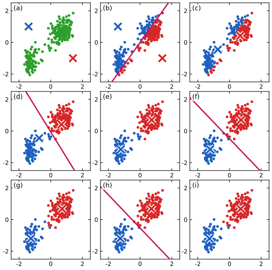
fig9_1. Download: PDF · SVG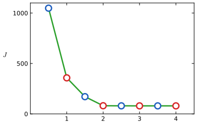
fig9_2. Download: PDF · SVGPractical remarks p. 427. Because of Result 9.1(c), K-means is usually run from several starts and the run with the smallest \(J\) is kept. Starting from \(K\) data points chosen at random is the simplest choice; spreading the initial points out (as in the "k-means++" seeding of Arthur and Vassilvitskii, 2007) is usually better. Since \(J\) uses Euclidean distance, the result depends on the units of the variables, which is why the Old Faithful data are standardised first. K-means is also the standard way to initialise EM for Gaussian mixtures (Section 9.2.2). Each E step compares every point with every prototype; tree data structures and the triangle inequality can skip most of these distance computations (the book cites Moore, 2000, and Elkan, 2003).
Sequential (on-line) K-means
When data arrive one at a time, MacQueen's (1967) version updates only the prototype nearest to the new point \(\mathbf{x}_n\):
\[ \bm\mu_k^{\rm new}=\bm\mu_k^{\rm old}+\eta_n\,(\mathbf{x}_n-\bm\mu_k^{\rm old}), \tag{9.5} \]where \(\eta_n\) is a learning rate that decreases as more data are seen.
Filling the gap 9.2: (9.5) is a Robbins–Monro step p. 427, (9.5); Exercise 9.2
The book says that (9.5) follows from the Robbins–Monro procedure of Section 2.3.5 "applied to the derivatives of \(J\)". We identify the regression function, the noisy observation and the step size, and show that the choice \(\eta=1/(\text{count})\) turns \(\bm\mu_k\) into a running mean.
Derivation
Robbins–Monro. To find a root \(\bm\theta^\star\) of a regression function \(\mathbf{f}(\bm\theta)\)
The regression function. Think of the data as an endless stream from a distribution \(p(\mathbf{x})\) with \(\E\lVert\mathbf{x}\rVert^2\)
For a fixed \(\mathbf{x}\) that is not equidistant from two prototypes (a set of probability one when \(p\) has a density and the prototypes are distinct), the minimum is attained by a single \(k\), so near \(\bm\mu\) the integrand equals \(\lVert\mathbf{x}-\bm\mu_k\rVert^2\) for that \(k\) and is differentiable, with \(\nabla_{\bm\mu_k}\)
This is the population form of (9.3): its root says that each prototype is the mean of its own Voronoi cell, \(\bm\mu_k\)
The update. The quantity \(\mathbf{z}\)
For every prototype other than the nearest one, \(r_k=0\) and nothing moves; the nearest one moves by (9.5) with \(\eta_n=2a_{n-1}\).
Running means. Give each prototype its own counter \(m_k\) of the points assigned to it so far and use \(\eta=1/m_k\) after incrementing the counter. If \(\bm\mu_k^{\rm old}\) is the mean of \(m-1\) points, then \(\bm\mu_k^{\rm old}+\frac1m(\mathbf{x}_n-\bm\mu_k^{\rm old})\)
K-medoids
Squared Euclidean distance is unsuitable for categorical variables and makes the means sensitive to outliers (one far-away point can drag a mean anywhere). Replacing it by a general dissimilarity \(\mathcal{V}(\mathbf{x},\mathbf{x}')\) gives the distortion
\[ \widetilde J=\sum_{n=1}^{N}\sum_{k=1}^{K} r_{nk}\,\mathcal{V}(\mathbf{x}_n,\bm\mu_k), \tag{9.6} \]minimised by the K-medoids algorithm. Its E step is again "assign each point to the prototype with the smallest dissimilarity". In the M step the prototype of each cluster is usually restricted to be one of the cluster's own points (its medoid), so that only evaluations of \(\mathcal{V}\) are needed (Kaufman and Rousseeuw, 1990).
Filling the gap 9.3: the cost and the convergence of K-medoids p. 428, (9.6)
The book states the costs \(O(KN)\) and \(O(N_k^2)\). We count them and check that the restricted M step still never increases \(\widetilde J\), so Result 9.1 carries over.
Derivation
Costs. E step: for each of the \(N\) points evaluate \(\mathcal{V}\) against the \(K\) prototypes, \(NK\) evaluations. M step for cluster \(k\) with \(N_k\) members: for each candidate medoid \(\mathbf{x}_m\) in the cluster, compute \(\sum_{n\in\mathcal{C}_k}\mathcal{V}(\mathbf{x}_n,\mathbf{x}_m)\), which takes \(N_k\) evaluations, and keep the candidate with the smallest sum; that is \(N_k^2\) evaluations, and \(\sum_kN_k^2\) in total (about \(N^2/K\) for balanced clusters, \(N^2\) in the worst case).
Monotonicity. Assume \(\mathcal{V}\ge0\) and \(\mathcal{V}(\mathbf{x},\mathbf{x})\)
A special case. If \(\mathcal{V}(\mathbf{x},\mathbf{x}')\)
Hard versus soft assignments p. 428. K-means assigns every point to exactly one cluster, even a point that lies almost halfway between two centres. The probabilistic treatment of Section 9.2 replaces the 0/1 indicators by posterior probabilities, which express how uncertain each assignment is.
9.1.1 Image segmentation and compression
pp. 428–430 Treat every pixel of a colour image as a point \((R,G,B)\in[0,1]^3\) and run K-means on these \(N\) points, ignoring where the pixels are in the image. Redrawing each pixel in the colour of its cluster centre represents the image with a palette of \(K\) colours (Figure 9.3). As a segmentation method this is crude, because neighbouring pixels are not encouraged to share a cluster; it simply shows what K-means does. (The colour cube is bounded rather than all of \(\R^3\), but nothing in the algorithm requires an unbounded space: means of colours are colours.)
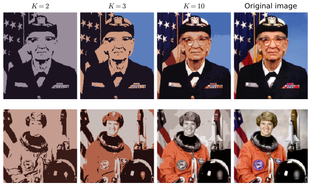
fig9_3. Download: PDF · SVGVector quantisation. The same output is a lossy compression scheme. Store, for every point, only the label \(k\) of its cluster, plus the \(K\) code-book vectors \(\bm\mu_k\); decode each point as its code-book vector. A new point is compressed by finding its nearest code-book vector. The mean squared reconstruction error is \(J/N\), so K-means is precisely the algorithm that designs a code book of size \(K\) to minimise this error for the given data; in quantisation theory it is Lloyd's algorithm (Lloyd, 1982; Gersho and Gray, 1992).
Filling the gap 9.4: the compression arithmetic p. 430
The book quotes 43,248, 86,472 and 173,040 bits for \(K=2,3,10\). We derive the general count and show where the rounding goes.
Derivation
Raw image. Each of the \(N\) pixels has three channels stored with 8 bits each: \(24N\) bits.
Compressed image. A fixed-length binary code for \(K\) labels needs \(b\) bits with \(2^b\ge K\), i.e. \(b=\lceil\log_2K\rceil\) bits per pixel. The code book holds \(K\) colours of 24 bits each. Total:
\[ B(K)=24K+N\lceil\log_2K\rceil \ \text{bits},\qquad \frac{B(K)}{24N}=\frac{K}{N}+\frac{\lceil\log_2K\rceil}{24}\ \longrightarrow\ \frac{\lceil\log_2K\rceil}{24}\quad(N\to\infty). \]The book writes \(24K+N\log_2K\) "rounding up to the nearest integer"; its numbers show that the rounding is applied per pixel. For the book's \(240\times180\) image, \(N=43{,}200\) and the raw image takes \(24\times43{,}200=1{,}036{,}800\) bits. Then \(B(2)=48+43{,}200=43{,}248\) (4.17%), \(B(3)=72+2\times43{,}200=86{,}472\) (8.34%) and \(B(10)\)
Doing better than \(\lceil\log_2K\rceil\). Coding labels in blocks removes the rounding loss: for \(K=3\), five labels have \(3^5=243\le2^8\) values, so 8 bits per block, 1.6 bits per label, close to \(\log_23\approx1.585\). If the clusters are used with frequencies \(N_k/N\), an entropy code needs only about \(N\,H\) bits for the labels, with \(H\)
9.2 Mixtures of Gaussians
pp. 430–432 Section 2.3.9 introduced the Gaussian mixture (2.188) as a weighted sum of Gaussian densities,
\[ p(\mathbf{x})=\sum_{k=1}^{K}\pi_k\,\N(\mathbf{x}\given\bm\mu_k,\bm\Sigma_k). \tag{9.7} \]The same distribution arises from a two-stage story: first pick a component at random, then draw \(\mathbf{x}\) from that component. Making the hidden choice an explicit random variable is what leads to EM.
Definition 9.2 (the Gaussian mixture as a latent-variable model)
Let \(\mathbf{z}=(z_1,\dots,z_K)^\T\) be a 1-of-K vector: \(z_k\in\{0,1\}\) and \(\sum_kz_k=1\), so \(\mathbf{z}\) takes the \(K\) values \(\mathbf{e}_1,\dots,\mathbf{e}_K\). Put \(p(z_k=1)=\pi_k\), where the mixing coefficients satisfy
\[ 0\le\pi_k\le1 \tag{9.8} \] \[ \sum_{k=1}^{K}\pi_k=1, \tag{9.9} \]and let \(\mathbf{x}\) given \(z_k=1\) be \(\N(\mathbf{x}\given\bm\mu_k,\bm\Sigma_k)\). Using the 1-of-K coding, both distributions can be written as products:
\[ p(\mathbf{z})=\prod_{k=1}^{K}\pi_k^{z_k} \tag{9.10} \] \[ p(\mathbf{x}\given\mathbf{z})=\prod_{k=1}^{K}\N(\mathbf{x}\given\bm\mu_k,\bm\Sigma_k)^{z_k}. \tag{9.11} \]This is the directed graph \(\mathbf{z}\to\mathbf{x}\) of Figure 9.4: the joint distribution is \(p(\mathbf{x},\mathbf{z})\)
Result 9.2 (marginal and posterior of the latent-variable model; Exercise 9.3)
Under Definition 9.2, (a) \(p(\mathbf{x},\mathbf{z})\)
(c) the posterior probability that \(\mathbf{x}\) came from component \(k\), the responsibility of component \(k\) for \(\mathbf{x}\), is
\[ \gamma(z_k)\equiv p(z_k=1\given\mathbf{x})=\frac{p(z_k=1)\,p(\mathbf{x}\given z_k=1)}{\sum_{j=1}^{K}p(z_j=1)\,p(\mathbf{x}\given z_j=1)}=\frac{\pi_k\,\N(\mathbf{x}\given\bm\mu_k,\bm\Sigma_k)}{\sum_{j=1}^{K}\pi_j\,\N(\mathbf{x}\given\bm\mu_j,\bm\Sigma_j)}. \tag{9.13} \]Proof
Everything rests on one observation: if \(\mathbf{z}=\mathbf{e}_j\) then \(z_k=1\) for \(k=j\) and \(z_k=0\) otherwise, so for any numbers \(a_1,\dots,a_K\), \(\prod_ka_k^{z_k}=a_j\) (every factor with \(z_k=0\) equals \(a_k^0=1\)).
(a) Multiply (9.10) and (9.11) and combine the two products over \(k\): \(\prod_k\pi_k^{z_k}\prod_k\N_k^{z_k}\)
(b) By the sum rule, \(p(\mathbf{x})\) is the sum of (a) over the \(K\) possible values \(\mathbf{z}=\mathbf{e}_j\), and by the observation above the term for \(\mathbf{e}_j\) is \(\pi_j\N_j\). Summing over \(j\) gives (9.12).
(c) Bayes' theorem: \(p(z_k=1\given\mathbf{x})\)
Reading the responsibilities. \(\pi_k\) is the prior probability of component \(k\) and \(\gamma(z_k)\) its posterior probability after seeing \(\mathbf{x}\). If all \(\pi_k\gt0\) then \(0\lt\gamma(z_k)\lt1\) (Gaussian densities are positive) and \(\sum_k\gamma(z_k)=1\). Writing \(a_k\)
Sampling. p. 432 The two-stage story gives a direct way to simulate from the mixture, an instance of ancestral sampling (Section 8.1.2): sample the parent \(\mathbf{z}\), then the child \(\mathbf{x}\).
Algorithm 9.2 (ancestral sampling from a Gaussian mixture)
- Draw \(u\sim\mathrm{Uniform}(0,1)\) and let \(k\) be the smallest index with \(\pi_1+\dots+\pi_k\ge u\); set \(\hat{\mathbf{z}}=\mathbf{e}_k\). Then \(P(\hat{\mathbf{z}}=\mathbf{e}_k)\)
\({}=\pi_k\): this happens exactly when \(u\) falls in the interval \((\pi_1+\dots+\pi_{k-1},\ \pi_1+\dots+\pi_k]\), whose length is \(\pi_k\). - Draw \(\bm\epsilon\sim\N(\mathbf{0},\mathbf{I}_D)\) and set \(\mathbf{x}\)
\({}=\bm\mu_k+\mathbf{L}_k\bm\epsilon\), where \(\mathbf{L}_k\mathbf{L}_k^\T\) \({}=\bm\Sigma_k\) (Cholesky factor). An affine image of a standard Gaussian vector is Gaussian with mean \(\bm\mu_k\) and covariance \(\mathbf{L}_k\mathbf{L}_k^\T\) \({}=\bm\Sigma_k\) (Gaussian facts). - The pair \((\mathbf{x},\hat{\mathbf{z}})\) is a draw from the joint \(p(\mathbf{z})p(\mathbf{x}\given\mathbf{z})\); keeping \(\mathbf{x}\) and discarding \(\hat{\mathbf{z}}\) gives a draw from the marginal (9.12).
In the language of Section 9.3, the pairs \(\{(\mathbf{x}_n,\mathbf{z}_n)\}\) form a complete data set and the \(\mathbf{x}_n\) alone an incomplete one. Figure 9.5 shows both, and also the responsibilities, which are the best we can say about the labels once they have been thrown away.
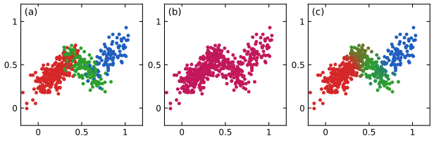
fig9_5. Download: PDF · SVG9.2.1 Maximum likelihood
pp. 432–435 Collect the observations in the \(N\times D\) matrix \(\mathbf{X}\) with rows \(\mathbf{x}_n^\T\), and the latent vectors in the \(N\times K\) matrix \(\mathbf{Z}\) with rows \(\mathbf{z}_n^\T\). If the pairs \((\mathbf{x}_n,\mathbf{z}_n)\) are independent and identically distributed (the plate diagram of Figure 9.6), the log likelihood of the observed data is, from (9.7),
\[ \ln p(\mathbf{X}\given\bm\pi,\bm\mu,\bm\Sigma)=\sum_{n=1}^{N}\ln\Big\{\sum_{k=1}^{K}\pi_k\,\N(\mathbf{x}_n\given\bm\mu_k,\bm\Sigma_k)\Big\}. \tag{9.14} \]Before maximising (9.14) we must face two features that a single Gaussian does not have: the likelihood can be made arbitrarily large, and every solution comes in \(K!\) copies.
Result 9.3 (the mixture likelihood is unbounded; a single Gaussian's is not) pp. 433–434, (9.15)
(a) Let \(K\ge2\). For any data set, (9.14) is unbounded above on \(\{\pi_k\)
(b) For a single Gaussian with covariance \(\sigma^2\mathbf{I}\), \(\ln p(\mathbf{X}\given\bm\mu,\sigma^2)\)
Proof
The singular term. A component centred on a data point contributes, at that point, the density
\[ \N(\mathbf{x}_n\given\mathbf{x}_n,\sigma_j^2\mathbf{I})=\frac{1}{(2\pi)^{D/2}}\,\frac{1}{\sigma_j^{D}}. \tag{9.15} \]Erratum. The book prints \(\frac{1}{(2\pi)^{1/2}}\frac{1}{\sigma_j}\), which is the case \(D=1\); the official errata replace \(\sigma_j\) by \(\sigma_j^D\), and for \(D\gt1\) the constant is also \((2\pi)^{D/2}\). The conclusion is the same: the term grows without bound as \(\sigma_j\to0\).
(a) Every term of (9.14) is the log of a sum of nonnegative numbers, so it is at least the log of any one of them. For \(n\ne n_0\) keep the term of component \(i\): \(\ln\sum_k\pi_k\N_{nk}\)
(b) For fixed \(\sigma^2\), \(\ln p\)
Why the collapse fails here: with \(\bm\mu=\mathbf{x}_{n_0}\), \(\ln p\)
Full covariance: \(\ln p\)
So maximum likelihood for Gaussian mixtures is, strictly speaking, ill-posed: the "best" fit puts a spike on a data point. Collapse onto lower-dimensional sets is also possible: with full covariance matrices a component can flatten onto any \(D\) or fewer data points, which always lie in a hyperplane (in two dimensions, onto the line through two points). In practice we look for a well-behaved local maximum instead, and guard against collapse: by detecting a shrinking component and resetting it (the book's suggestion), by a floor on the variances, by a prior (a MAP estimate, Section 9.3), or by the Bayesian treatment of Chapter 10, where the problem disappears. The phenomenon goes back at least to Kiefer and Wolfowitz (1956); bounding the ratio of the component variances makes the constrained likelihood bounded (Hathaway, 1985).
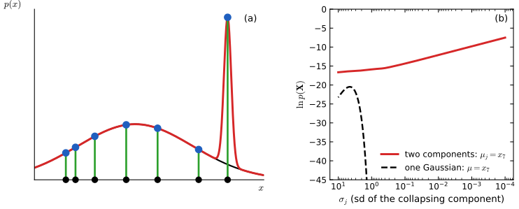
fig9_7. Download: PDF · SVGResult 9.4 (\(K!\) equivalent solutions) pp. 434–435
For a permutation \(\tau\) of \(\{1,\dots,K\}\) let \(\bm\theta_\tau\) give component \(k\) the parameters \((\pi_{\tau(k)},\bm\mu_{\tau(k)},\bm\Sigma_{\tau(k)})\). Then \(p(\mathbf{x}\given\bm\theta_\tau)\)
Proof
\(p(\mathbf{x}\given\bm\theta_\tau)\)
Consequences. The likelihood surface of a mixture with \(K\ge2\) is multimodal by symmetry alone. The parameters are at best identifiable up to relabelling: for finite Gaussian mixtures with distinct components and positive weights, equality of the densities does imply equality of the parameter sets up to a permutation (Teicher, 1963; Yakowitz and Spragins, 1968). At degenerate points (two equal components, or some \(\pi_k=0\)) whole continua of parameters give the same density. For density estimation none of this matters; for interpreting fitted components one reports label-free summaries or fixes an ordering. In a Bayesian treatment the posterior has \(K!\) symmetric modes, which is why the variational lower bound used for comparing values of \(K\) in Chapter 10 gets a \(\ln K!\) correction (Section 10.2.4).
Why there is no closed form p. 435. For a single Gaussian the logarithm acts directly on an exponential and the likelihood equations are linear in the mean. In (9.14) the logarithm acts on a sum, and the stationarity conditions derived in the next section involve the responsibilities, which depend on all the parameters through the ratio (9.13). The result is a coupled system of transcendental equations. No general closed-form solution is known, and none could be a single formula, because the system typically has many solutions (at least \(K!\) maxima by Result 9.4, plus saddle points such as the one where all components coincide). One option is a general-purpose gradient method (as for the mixture density networks of Chapter 5); EM is the other.
9.2.2 EM for Gaussian mixtures
pp. 435–439 At an interior maximum of (9.14) (all \(\pi_k\gt0\), all \(\bm\Sigma_k\) positive definite) the derivatives with respect to every parameter vanish. Working them out gives three conditions in which the responsibilities appear by themselves. For the means:
\[ 0=\sum_{n=1}^{N}\underbrace{\frac{\pi_k\,\N(\mathbf{x}_n\given\bm\mu_k,\bm\Sigma_k)}{\sum_j\pi_j\,\N(\mathbf{x}_n\given\bm\mu_j,\bm\Sigma_j)}}_{\gamma(z_{nk})}\,\bm\Sigma_k^{-1}(\mathbf{x}_n-\bm\mu_k), \tag{9.16} \] \[ \bm\mu_k=\frac{1}{N_k}\sum_{n=1}^{N}\gamma(z_{nk})\,\mathbf{x}_n, \tag{9.17} \] \[ N_k=\sum_{n=1}^{N}\gamma(z_{nk}). \tag{9.18} \]\(N_k\) is the effective number of points assigned to component \(k\), and (9.17) is a weighted mean in which point \(n\) has weight \(\gamma(z_{nk})\).
Filling the gap 9.5: the derivative with respect to a mean p. 435, (9.16)–(9.17)
The book quotes (9.16) using "the form (2.43) for the Gaussian". Here is the chain rule in full, and the correction of an erratum in early printings.
Derivation
From (2.43),
\[ \ln\N(\mathbf{x}\given\bm\mu,\bm\Sigma)=-\frac D2\ln(2\pi)-\frac12\ln|\bm\Sigma|-\frac12(\mathbf{x}-\bm\mu)^\T\bm\Sigma^{-1}(\mathbf{x}-\bm\mu). \]Since \(\nabla_{\mathbf{u}}(\mathbf{u}^\T\mathbf{A}\mathbf{u})\)
Only one term of the inner sum of (9.14) contains \(\bm\mu_k\), so by the chain rule
\[ \nabla_{\bm\mu_k}\ln\Big\{\sum_j\pi_j\N_{nj}\Big\}=\frac{\pi_k\nabla_{\bm\mu_k}\N_{nk}}{\sum_j\pi_j\N_{nj}}=\frac{\pi_k\N_{nk}}{\sum_j\pi_j\N_{nj}}\,\bm\Sigma_k^{-1}(\mathbf{x}_n-\bm\mu_k)=\gamma_{nk}\,\bm\Sigma_k^{-1}(\mathbf{x}_n-\bm\mu_k). \]Summing over \(n\) and setting the result to zero is (9.16). Multiply on the left by \(\bm\Sigma_k\) (invertible): \(\sum_n\gamma_{nk}(\mathbf{x}_n-\bm\mu_k)\)
Erratum. Early printings of (9.16) carry an extra minus sign and \(\bm\Sigma_k\) in place of \(\bm\Sigma_k^{-1}\), and the next sentence then multiplies by \(\bm\Sigma_k^{-1}\); the form above, with "multiplying by \(\bm\Sigma_k\)", is the corrected one. Note that (9.17) is not an explicit formula: \(\bm\mu_k\) also appears inside every \(\gamma_{nk}\). ∎
For the covariances the same reasoning, together with the maximum likelihood covariance of a single Gaussian (Section 2.3.4), gives
\[ \bm\Sigma_k=\frac{1}{N_k}\sum_{n=1}^{N}\gamma(z_{nk})\,(\mathbf{x}_n-\bm\mu_k)(\mathbf{x}_n-\bm\mu_k)^\T, \tag{9.19} \]a weighted sample covariance with the effective count \(N_k\) in the denominator.
Filling the gap 9.6: the derivative with respect to a covariance matrix p. 436, (9.19)
The book gives (9.19) after "following a similar line of reasoning". We derive it with differentials, the trace trick and the derivative of a log-determinant, working with the precision matrix and taking care of the symmetry constraint.
Derivation
Parametrise by the precision. Let \(\bm\Lambda_k=\bm\Sigma_k^{-1}\). The map \(\bm\Sigma\mapsto\bm\Sigma^{-1}\) is a smooth bijection of the positive definite matrices onto themselves, with smooth inverse, so the stationary points in \(\bm\Sigma_k\) are exactly the images of the stationary points in \(\bm\Lambda_k\). With the trace trick \(\mathbf{u}^\T\bm\Lambda\mathbf{u}\)
Differential. Perturb \(\bm\Lambda\) by a small symmetric matrix \(\d\bm\Lambda\) (the precision must stay symmetric). Jacobi's formula gives \(\d\ln|\bm\Lambda|\)
Chain rule through the mixture. As in the previous box, \(\d\ln\sum_j\pi_j\N_{nj}\)
Stationarity. At a stationary point this differential is zero for every symmetric \(\d\bm\Lambda_k\). The matrix \(\mathbf{G}_k\) is itself symmetric, so we may take \(\d\bm\Lambda_k=\mathbf{G}_k\): then \(\Tr(\mathbf{G}_k^2)\)
Which mean? At a stationary point (9.17) and (9.19) hold simultaneously, so the \(\bm\mu_k\) in (9.19) is the one from (9.17). In the algorithm below one therefore computes the new means first and uses them in the covariances. ∎
For the mixing coefficients the constraint (9.9) must be respected. Following Appendix E, maximise the Lagrangian
\[ \ln p(\mathbf{X}\given\bm\pi,\bm\mu,\bm\Sigma)+\lambda\Big(\sum_{k=1}^{K}\pi_k-1\Big), \tag{9.20} \]whose derivative with respect to \(\pi_k\) gives
\[ 0=\sum_{n=1}^{N}\frac{\N(\mathbf{x}_n\given\bm\mu_k,\bm\Sigma_k)}{\sum_j\pi_j\,\N(\mathbf{x}_n\given\bm\mu_j,\bm\Sigma_j)}+\lambda, \tag{9.21} \]and then, with \(\lambda=-N\),
\[ \pi_k=\frac{N_k}{N}: \tag{9.22} \]the mixing coefficient of a component is its average responsibility.
Filling the gap 9.7: the Lagrange multiplier is \(\lambda=-N\) p. 436, (9.20)–(9.22)
The book says "multiply both sides by \(\pi_k\) and sum over \(k\)". We do so, check the inequality constraints, and confirm the answer with an unconstrained parametrisation.
Derivation
Lagrange. Only the \(k\)th term of each inner sum contains \(\pi_k\), so \(\partial/\partial\pi_k\) of (9.20) is \(\sum_n\N_{nk}/\sum_j\pi_j\N_{nj}+\lambda\), which is (9.21). At an interior point \(\pi_k\gt0\), so multiplying (9.21) by \(\pi_k\) loses nothing:
\[ 0=\sum_n\frac{\pi_k\N_{nk}}{\sum_j\pi_j\N_{nj}}+\lambda\pi_k=N_k+\lambda\pi_k\qquad(k=1,\dots,K). \]Sum over \(k\). For every \(n\) the responsibilities add up to one, \(\sum_k\gamma_{nk}=1\), so \(\sum_kN_k\)
Check without a multiplier. Write \(\pi_k=e^{\eta_k}/\sum_je^{\eta_j}\), which satisfies (9.8) and (9.9) for every real \(\bm\eta\). Then \(\partial\pi_j/\partial\eta_k\)
which vanishes exactly when \(\pi_k=N_k/N\). ∎
Result 9.5 (the likelihood equations are fixed-point equations) p. 436
Let \(\bm\theta\) have all \(\pi_k\gt0\) and all \(\bm\Sigma_k\) positive definite. Then \(\bm\theta\) is a stationary point of (9.14) (subject to (9.9)) if and only if (9.17), (9.19) and (9.22) hold when the responsibilities on their right-hand sides are computed from \(\bm\theta\) itself by (9.13). Equivalently: the interior stationary points of the likelihood are exactly the fixed points of the map "compute the responsibilities from \(\bm\theta\), then apply (9.17), (9.19), (9.22)", which is one cycle of the EM algorithm below.
Proof
Each step of the three gap boxes is an equivalence. The gradient with respect to \(\bm\mu_k\) vanishes if and only if (9.17) holds (multiplication by the invertible \(\bm\Sigma_k\) is reversible). Given that, the derivative with respect to \(\bm\Lambda_k\) vanishes if and only if \(\mathbf{G}_k=\mathbf{0}\), i.e. (9.19). The constrained stationarity condition for \(\bm\pi\) (gradient of the Lagrangian zero for some \(\lambda\)) holds if and only if (9.22). In all three, \(\gamma_{nk}\) is evaluated at the same \(\bm\theta\), which is exactly the statement that \(\bm\theta\) is mapped to itself. ∎
Two warnings. First, (9.17), (9.19) and (9.22) are not a closed-form solution: the responsibilities on the right depend on the unknowns. Second, fixed points need not be maxima: if all components are identical (\(\bm\mu_k=\bar{\mathbf{x}}\), \(\bm\Sigma_k=\mathbf{S}\), any \(\bm\pi\)), then every \(\gamma_{nk}=\pi_k\) and one EM cycle returns the same parameters; this symmetric point is usually a saddle (compare Exercise 9.13). What the equations do suggest is to iterate them, and Section 9.4 proves that the iteration never decreases the likelihood.
Algorithm 9.3 (EM for Gaussian mixtures) pp. 438–439
- Initialise \(\bm\mu_k\), \(\bm\Sigma_k\), \(\pi_k\) and evaluate the log likelihood (9.28).
- E step. Evaluate the responsibilities with the current parameters: \[ \gamma(z_{nk})=\frac{\pi_k\,\N(\mathbf{x}_n\given\bm\mu_k,\bm\Sigma_k)}{\sum_{j=1}^{K}\pi_j\,\N(\mathbf{x}_n\given\bm\mu_j,\bm\Sigma_j)}. \tag{9.23} \]
- M step. Re-estimate the parameters with these responsibilities, the means first: \[ \bm\mu_k^{\rm new}=\frac{1}{N_k}\sum_{n=1}^{N}\gamma(z_{nk})\,\mathbf{x}_n \tag{9.24} \] \[ \bm\Sigma_k^{\rm new}=\frac{1}{N_k}\sum_{n=1}^{N}\gamma(z_{nk})\,(\mathbf{x}_n-\bm\mu_k^{\rm new})(\mathbf{x}_n-\bm\mu_k^{\rm new})^\T \tag{9.25} \] \[ \pi_k^{\rm new}=\frac{N_k}{N} \tag{9.26} \] where \[ N_k=\sum_{n=1}^{N}\gamma(z_{nk}). \tag{9.27} \]
- Evaluate the log likelihood \[ \ln p(\mathbf{X}\given\bm\mu,\bm\Sigma,\bm\pi)=\sum_{n=1}^{N}\ln\Big\{\sum_{k=1}^{K}\pi_k\,\N(\mathbf{x}_n\given\bm\mu_k,\bm\Sigma_k)\Big\} \tag{9.28} \] and stop if it (or the parameters) changed by less than a tolerance; otherwise return to step 2.
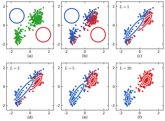
fig9_8. Download: PDF · SVGPractical points p. 438
- Initialisation. EM needs many more iterations than K-means, each of them more expensive. A common recipe: run K-means first, then set \(\bm\mu_k\) to the cluster means, \(\bm\Sigma_k\) to the within-cluster sample covariances and \(\pi_k\) to the cluster fractions. Several starts are advisable; keep the best non-degenerate solution, since EM finds a local maximum that depends on the start.
- Computing in log space. Evaluate \(\ln\N\) through a Cholesky factor (\(\ln|\bm\Sigma|=2\sum_i\ln L_{ii}\), the quadratic form by a triangular solve), and the responsibilities as a softmax of \(a_{nk}=\ln\pi_k+\ln\N_{nk}\) with the log-sum-exp trick. The same normaliser gives (9.28) for free: \(\ln p(\mathbf{X}\given\bm\theta)\)
\({}=\sum_n\ln\sum_ke^{a_{nk}}\). - Guarding against singularities. Add a small multiple of the identity to each \(\bm\Sigma_k\) after the M step (a variance floor), reset a component whose \(N_k\) or \(|\bm\Sigma_k|\) becomes tiny, or use a prior (the Wishart example in Section 9.3 is the principled version of the floor).
- Monitoring. The log likelihood must not decrease from one cycle to the next (Result 9.15); a decrease signals a bug (or a variance floor, which changes the objective). Convergence can be very slow when components overlap (Result 9.17).
- Cost. One cycle costs \(O(NKD^2)\) for the quadratic forms and the covariance updates plus \(O(KD^3)\) for the factorisations.
9.3 An alternative view of EM
pp. 439–441 Now let \(\mathbf{X}\) be all the observed data, \(\mathbf{Z}\) all the latent variables (row \(\mathbf{z}_n^\T\) for observation \(n\)) and \(\bm\theta\) all the parameters. The log likelihood is
\[ \ln p(\mathbf{X}\given\bm\theta)=\ln\Big\{\sum_{\mathbf{Z}}p(\mathbf{X},\mathbf{Z}\given\bm\theta)\Big\}, \tag{9.29} \]with the sum replaced by an integral for continuous latent variables. The sum inside the logarithm is the whole difficulty: even when the joint distribution \(p(\mathbf{X},\mathbf{Z}\given\bm\theta)\) is a simple exponential-family distribution, its marginal usually is not, and the logarithm can no longer undo the exponential.
Definition 9.3 (complete data and the \(Q\) function)
\(\{\mathbf{X},\mathbf{Z}\}\) is the complete data and \(\mathbf{X}\) the incomplete (actually observed) data; \(\ln p(\mathbf{X},\mathbf{Z}\given\bm\theta)\) is the complete-data log likelihood, which we assume easy to maximise. What we know about \(\mathbf{Z}\) is its posterior \(p(\mathbf{Z}\given\mathbf{X},\bm\theta)\). Given a current value \(\bm\theta^{\rm old}\), the expected complete-data log likelihood is
\[ Q(\bm\theta,\bm\theta^{\rm old})=\sum_{\mathbf{Z}}p(\mathbf{Z}\given\mathbf{X},\bm\theta^{\rm old})\,\ln p(\mathbf{X},\mathbf{Z}\given\bm\theta), \tag{9.30} \]a function of the free argument \(\bm\theta\); the posterior weights are frozen at \(\bm\theta^{\rm old}\). The M step chooses
\[ \bm\theta^{\rm new}=\argmax_{\bm\theta}\ Q(\bm\theta,\bm\theta^{\rm old}). \tag{9.31} \]Algorithm 9.4 (the general EM algorithm) pp. 440–441
- Choose an initial \(\bm\theta^{\rm old}\).
- E step. Evaluate \(p(\mathbf{Z}\given\mathbf{X},\bm\theta^{\rm old})\).
- M step. Evaluate \[ \bm\theta^{\rm new}=\argmax_{\bm\theta}\ Q(\bm\theta,\bm\theta^{\rm old}) \tag{9.32} \] where \[ Q(\bm\theta,\bm\theta^{\rm old})=\sum_{\mathbf{Z}}p(\mathbf{Z}\given\mathbf{X},\bm\theta^{\rm old})\,\ln p(\mathbf{X},\mathbf{Z}\given\bm\theta). \tag{9.33} \]
- If the log likelihood or the parameters have not converged, set \[ \bm\theta^{\rm old}\leftarrow\bm\theta^{\rm new} \tag{9.34} \] and return to step 2.
Filling the gap 9.8: why the expected complete-data log likelihood? p. 440
The book admits that "the use of the expectation may seem somewhat arbitrary" and defers the reason to Section 9.4. Here is the reason in four lines; Section 9.4 develops it further.
Derivation
Let \(q(\mathbf{Z})\)
where \(\mathrm{H}[q]=-\sum'q\ln q\) does not depend on \(\bm\theta\). At \(\bm\theta=\bm\theta^{\rm old}\) both inequalities are equalities: \(p(\mathbf{X},\mathbf{Z}\given\bm\theta^{\rm old})/q(\mathbf{Z})\)
Any \(\bm\theta\) that raises \(Q\) raises the log likelihood by at least as much; the M step raises \(Q\) as far as it can. ∎
The M step is tractable because, in (9.30), the logarithm acts on the joint distribution. When the complete-data model is an exponential family this has a simple and general form.
Result 9.6 (EM for exponential-family complete data) pp. 439, 452
Suppose \(p(\mathbf{X},\mathbf{Z}\given\bm\eta)\)
so the E step needs only the expected complete-data sufficient statistics \(\bar{\mathbf{u}}\), and the M step is the complete-data maximum likelihood problem with \(\mathbf{u}\) replaced by \(\bar{\mathbf{u}}\): it solves the moment-matching equation \(\E_{\bm\eta}[\mathbf{u}(\mathbf{X},\mathbf{Z})]\)
Proof
Take the logarithm: \(\ln p(\mathbf{X},\mathbf{Z}\given\bm\eta)\)
For the Gaussian mixture, the complete-data log likelihood (9.36) below is, for each \(k\), linear in \(\sum_nz_{nk}\), \(\sum_nz_{nk}\mathbf{x}_n\) and \(\sum_nz_{nk}\mathbf{x}_n\mathbf{x}_n^\T\) (expand the quadratic form). Their expectations are \(N_k\), \(\sum_n\gamma_{nk}\mathbf{x}_n\) and \(\sum_n\gamma_{nk}\mathbf{x}_n\mathbf{x}_n^\T\), which are exactly the quantities from which (9.24)–(9.27) are computed. (The mixing weights satisfy the constraint (9.9), so this is a constrained version of the result, handled by the Lagrange argument.)
MAP estimation. p. 441 With a prior \(p(\bm\theta)\) the same algorithm finds a mode of the posterior \(p(\bm\theta\given\mathbf{X})\): the E step is unchanged and the M step maximises \(Q(\bm\theta,\bm\theta^{\rm old})+\ln p(\bm\theta)\). A suitable prior removes the singularities of Section 9.2.1.
Filling the gap 9.9: the MAP version, and a prior that prevents collapse p. 441; Exercise 9.4
We show why only the M step changes, and work out the M step for a Wishart prior on each precision matrix, which keeps every covariance bounded away from singular.
Derivation
Only the M step changes. By Bayes' theorem \(\ln p(\bm\theta\given\mathbf{X})\)
with equality at \(\bm\theta^{\rm old}\). So maximising \(Q+\ln p(\bm\theta)\) increases the log posterior, by the argument of that box (and of (9.77) in Section 9.4).
Wishart prior on the precisions. Take independent Wishart priors (B.78) on the precisions, and no prior on the means:
\[ p(\bm\Lambda_k)=\Wish(\bm\Lambda_k\given\mathbf{W}_0,\nu_0)\propto|\bm\Lambda_k|^{(\nu_0-D-1)/2}\exp\Big\{-\frac12\Tr(\mathbf{W}_0^{-1}\bm\Lambda_k)\Big\}. \] The \(\bm\mu_k\)-part of the M step is unchanged, (9.24), and does not depend on \(\bm\Lambda_k\). With \(\widetilde{\mathbf{S}}_k\)
When \(c=N_k+\nu_0-D-1\gt0\), this is strictly concave in \(\bm\Lambda_k\) (see the proof of Result 9.8), and the differential calculation of the covariance gap box gives its unique maximiser
\[ \bm\Sigma_k^{\rm new}=(\bm\Lambda_k^{\rm new})^{-1}=\frac{\widetilde{\mathbf{S}}_k+\mathbf{W}_0^{-1}}{N_k+\nu_0-D-1}. \]If \(\nu_0\gt D+1\), the denominator is positive for every \(N_k\ge0\), and since \(\widetilde{\mathbf{S}}_k\) is positive semidefinite and \(N_k\le N\), \(\bm\Sigma_k^{\rm new}-\mathbf{W}_0^{-1}/(N+\nu_0-D-1)\) is positive semidefinite: no component can collapse, however few points it explains. A Dirichlet prior \(\Dir(\bm\pi\given\bm\alpha)\) on the weights similarly gives \(\pi_k^{\rm new}\)
Missing data. p. 441 The unobserved variables need not be labels: EM also handles data sets in which some values are missing, by treating the missing values as \(\mathbf{Z}\). This maximises the likelihood of the observed values, which is the right thing to do when the data are missing at random: whether a value is missing may depend on the observed values, but not on the missing value itself. A sensor that fails to report whenever the true value exceeds a threshold violates this, and ignoring the mechanism then biases the estimates (here downwards).
Filling the gap 9.10: why "missing at random" makes it legitimate to ignore the missingness p. 441
The book states the condition; here is the factorisation of the likelihood that justifies it (Rubin, 1976; Little and Rubin, 2019).
Derivation
Split the full data matrix as \(\mathbf{Y}\)
Missing at random means \(p(\mathbf{R}\given\mathbf{Y}_{\rm obs},\mathbf{Y}_{\rm mis},\bm\phi)\)
If, in addition, \(\bm\theta\) and \(\bm\phi\) vary independently (no constraint links them), maximising the full likelihood over \(\bm\theta\) is the same as maximising \(p(\mathbf{Y}_{\rm obs}\given\bm\theta)\): the mechanism is ignorable, and EM with \(\mathbf{Z}=\mathbf{Y}_{\rm mis}\) maximises the right function. In the threshold example the indicator depends on the value that is missing, the factorisation fails, and \(p(\mathbf{Y}_{\rm obs}\given\bm\theta)\) treats the surviving (small) values as representative, so the mean is underestimated. ∎
Example: EM for a Gaussian with missing entries
Let \(\mathbf{x}_n\sim\N(\bm\mu,\bm\Sigma)\) independently, with some entries missing at random. For row \(n\) let \(o\) and \(m\) index its observed and missing coordinates. E step (conditional Gaussian): fill in \(\hat{\mathbf{x}}_{n,m}\)
Derivation
The complete-data log likelihood is
\[ -\frac N2\ln|\bm\Sigma|-\frac12\sum_n(\mathbf{x}_n-\bm\mu)^\T\bm\Sigma^{-1}(\mathbf{x}_n-\bm\mu)+\const . \]Under the posterior of the missing entries (rows are independent, so row \(n\) only involves its own conditional distribution), \(\mathbf{x}_n\) has mean \(\hat{\mathbf{x}}_n\) and covariance \(\mathbf{C}_n\), so by the expected quadratic form (toolkit, trace identities (c))
\[ \E\big[(\mathbf{x}_n-\bm\mu)^\T\bm\Sigma^{-1}(\mathbf{x}_n-\bm\mu)\big]=(\hat{\mathbf{x}}_n-\bm\mu)^\T\bm\Sigma^{-1}(\hat{\mathbf{x}}_n-\bm\mu)+\Tr(\bm\Sigma^{-1}\mathbf{C}_n). \]Hence
\[ Q=-\frac N2\ln|\bm\Sigma|-\frac12\Tr\Big(\bm\Sigma^{-1}\sum_n\big\{(\hat{\mathbf{x}}_n-\bm\mu)(\hat{\mathbf{x}}_n-\bm\mu)^\T+\mathbf{C}_n\big\}\Big)+\const , \]the single-Gaussian likelihood of the filled-in data, with the scatter matrix enlarged by \(\sum_n\mathbf{C}_n\). Maximising over \(\bm\mu\) gives the mean of the \(\hat{\mathbf{x}}_n\) (the \(\mathbf{C}_n\) do not involve \(\bm\mu\)); maximising over \(\bm\Sigma\) as in the covariance gap box gives the stated \(\bm\Sigma^{\rm new}\). ∎
9.3.1 Gaussian mixtures revisited
pp. 441–443 Suppose that, besides \(\mathbf{X}\), we were told which component generated each point (the complete data of Figure 9.5(a), graph in Figure 9.9). From (9.10) and (9.11) the complete-data likelihood is
\[ p(\mathbf{X},\mathbf{Z}\given\bm\mu,\bm\Sigma,\bm\pi)=\prod_{n=1}^{N}\prod_{k=1}^{K}\pi_k^{z_{nk}}\,\N(\mathbf{x}_n\given\bm\mu_k,\bm\Sigma_k)^{z_{nk}}, \tag{9.35} \] \[ \ln p(\mathbf{X},\mathbf{Z}\given\bm\mu,\bm\Sigma,\bm\pi)=\sum_{n=1}^{N}\sum_{k=1}^{K}z_{nk}\big\{\ln\pi_k+\ln\N(\mathbf{x}_n\given\bm\mu_k,\bm\Sigma_k)\big\}. \tag{9.36} \]Compared with (9.14), the sum over \(k\) and the logarithm have changed places, and the logarithm now acts directly on each Gaussian. The maximisation splits into \(K\) single-Gaussian fits and
\[ \pi_k=\frac1N\sum_{n=1}^{N}z_{nk}. \tag{9.37} \]Filling the gap 9.11: the complete-data likelihood and its maximisation p. 442, (9.35)–(9.37); Exercise 9.7
We derive (9.35) from the i.i.d. assumption and show that its maximiser is "fit each component to its own points", with a proof that the mixing coefficients are a global maximum.
Derivation
(9.35)–(9.36). The pairs \((\mathbf{x}_n,\mathbf{z}_n)\) are independent, so \(p(\mathbf{X},\mathbf{Z}\given\bm\theta)\)
Splitting. Let \(\mathcal{C}_k=\{n:z_{nk}=1\}\) and \(N_k=|\mathcal{C}_k|\). Each point belongs to exactly one group, so (9.36) equals
\[ \sum_{k=1}^{K}N_k\ln\pi_k+\sum_{k=1}^{K}\ \sum_{n\in\mathcal{C}_k}\ln\N(\mathbf{x}_n\given\bm\mu_k,\bm\Sigma_k). \]The pair \((\bm\mu_k,\bm\Sigma_k)\) appears only in the \(k\)th inner sum, the log likelihood of a single Gaussian for the points of group \(k\); its maximiser is the group mean and the group covariance with divisor \(N_k\) (2.121)–(2.122), provided that covariance is nonsingular.
Mixing coefficients, globally. With \(p_k=N_k/N\), Gibbs' inequality (KL divergence) gives, for every \(\bm\pi\) satisfying (9.8) and (9.9),
\[ \sum_kN_k\ln\pi_k=N\sum_kp_k\ln p_k-N\,\KL(\mathbf{p}\|\bm\pi)\ \le\ N\sum_kp_k\ln p_k, \]with equality if and only if \(\bm\pi=\mathbf{p}\), which is (9.37). The Lagrange calculation of the mixing-coefficient box, with \(\gamma_{nk}\) replaced by \(z_{nk}\), finds the same point but only as a stationary point; the inequality shows it is the global maximum. ∎
We do not observe \(\mathbf{Z}\), so we average (9.36) over its posterior. From (9.35) and Bayes' theorem,
\[ p(\mathbf{Z}\given\mathbf{X},\bm\mu,\bm\Sigma,\bm\pi)\propto\prod_{n=1}^{N}\prod_{k=1}^{K}\big[\pi_k\,\N(\mathbf{x}_n\given\bm\mu_k,\bm\Sigma_k)\big]^{z_{nk}}. \tag{9.38} \]Result 9.7 (the posterior over \(\mathbf{Z}\) factorises; Exercise 9.5) p. 443, (9.38)–(9.39)
Under (9.38) the \(\mathbf{z}_n\) are independent given \(\mathbf{X}\), \(p(\mathbf{Z}\given\mathbf{X},\bm\theta)\)
Proof
Factorisation. \(p(\mathbf{Z}\given\mathbf{X},\bm\theta)\)
The same by d-separation. In Figure 9.6, treat \(\bm\pi\), \(\bm\mu\), \(\bm\Sigma\) as fixed (conditioned on). Every path from \(\mathbf{z}_n\) to \(\mathbf{z}_m\), \(m\ne n\), passes through one of these parameter nodes with both edges pointing away from it (tail to tail: \(\mathbf{z}_n\leftarrow\bm\pi\)
The expectation. By the factorisation, \(\E[z_{nk}]\) involves only the distribution of \(\mathbf{z}_n\): the factors for \(m\ne n\) sum to the same constant in the numerator and the denominator and cancel, which leaves the first expression in (9.39). The sums run over the \(K\) values \(\mathbf{z}_n=\mathbf{e}_j\); in the numerator only \(\mathbf{z}_n=\mathbf{e}_k\) has \(z_{nk}\ne0\), and its product equals \(\pi_k\N_{nk}\) (the 1-of-K observation in the proof of Result 9.2); the denominator is \(\sum_j\pi_j\N_{nj}\). (Early printings write the first line of (9.39) differently; the form above is the corrected one.) ∎
Since (9.36) is linear in the \(z_{nk}\), its expectation is obtained by replacing each \(z_{nk}\) by \(\E[z_{nk}]=\gamma(z_{nk})\):
\[ \E_{\mathbf{Z}}\big[\ln p(\mathbf{X},\mathbf{Z}\given\bm\mu,\bm\Sigma,\bm\pi)\big]=\sum_{n=1}^{N}\sum_{k=1}^{K}\gamma(z_{nk})\big\{\ln\pi_k+\ln\N(\mathbf{x}_n\given\bm\mu_k,\bm\Sigma_k)\big\}. \tag{9.40} \]Here the responsibilities are computed from the old parameters (E step), while the parameters inside the braces are free. Maximising over them (M step) gives back the updates (9.17), (9.19), (9.22), but now in a stronger sense.
Result 9.8 (the M step maximises (9.40) exactly; Exercises 9.8 and 9.9)
Hold the responsibilities fixed, and suppose that \(N_k\gt0\) and that \(\widetilde{\mathbf{S}}_k\)
Proof
Write (9.40) as \(\sum_kN_k\ln\pi_k+\sum_kQ_k(\bm\mu_k,\bm\Lambda_k)\), where, with \(\bm\Lambda_k=\bm\Sigma_k^{-1}\) and up to constants,
\[ Q_k(\bm\mu,\bm\Lambda)=\frac{N_k}{2}\ln|\bm\Lambda|-\frac12\sum_n\gamma_{nk}(\mathbf{x}_n-\bm\mu)^\T\bm\Lambda(\mathbf{x}_n-\bm\mu). \]The three groups of parameters can be maximised separately.
(i) Mixing coefficients. By the Gibbs-inequality argument of the previous gap box, with \(p_k=N_k/N\), the unique maximiser is \(\pi_k=N_k/N\).
(ii) Means (Exercise 9.8). Fix \(\bm\Lambda\) positive definite. The gradient of \(Q_k\) in \(\bm\mu\) is \(\bm\Lambda\sum_n\gamma_{nk}(\mathbf{x}_n-\bm\mu)\) and the Hessian is \(-N_k\bm\Lambda\), negative definite. So \(Q_k(\cdot,\bm\Lambda)\) is strictly concave with unique maximiser \(\bm\mu_k^{\rm new}\)
(iii) Precisions (Exercise 9.9). By the trace trick, \(f(\bm\Lambda)\)
Unboundedness. If \(\widetilde{\mathbf{S}}_k\mathbf{v}\)
Combining (i)–(iii): for every admissible parameter value, (9.40) is at most its value at the EM update, with equality only there. Contrast with Section 9.2.2, where the same formulas were only necessary conditions, because there the responsibilities moved with the parameters. ∎
9.3.2 Relation to K-means
pp. 443–444 K-means makes hard assignments, EM soft ones. To connect them, give every component the same covariance \(\epsilon\mathbf{I}\), with \(\epsilon\) a fixed constant (not re-estimated):
\[ p(\mathbf{x}\given\bm\mu_k,\bm\Sigma_k)=\frac{1}{(2\pi\epsilon)^{D/2}}\exp\Big\{-\frac{1}{2\epsilon}\lVert\mathbf{x}-\bm\mu_k\rVert^2\Big\}. \tag{9.41} \]Erratum. The book prints \((2\pi\epsilon)^{M/2}\); the dimension of \(\mathbf{x}\) is \(D\). The responsibilities (9.13) become
\[ \gamma(z_{nk})=\frac{\pi_k\exp\{-\lVert\mathbf{x}_n-\bm\mu_k\rVert^2/2\epsilon\}}{\sum_j\pi_j\exp\{-\lVert\mathbf{x}_n-\bm\mu_j\rVert^2/2\epsilon\}}, \tag{9.42} \]a softmax of the negative squared distances at "temperature" \(2\epsilon\). As \(\epsilon\to0\) they harden into the K-means assignments (9.2), and the expected complete-data log likelihood becomes, up to a scale factor and constants,
\[ \E_{\mathbf{Z}}\big[\ln p(\mathbf{X},\mathbf{Z}\given\bm\mu,\bm\Sigma,\bm\pi)\big]\ \to\ -\frac12\sum_{n=1}^{N}\sum_{k=1}^{K}r_{nk}\,\lVert\mathbf{x}_n-\bm\mu_k\rVert^2+\const. \tag{9.43} \]The next result says precisely in what sense (9.43) holds.
Result 9.9 (K-means is the small-variance limit of EM; Exercise 9.11) p. 444, (9.42)–(9.43)
Fix \(\pi_1,\dots,\pi_K\gt0\) and centres \(\bm\mu_1,\dots,\bm\mu_K\), and let \(\epsilon\to0\).
(a) If \(\mathbf{x}_n\) has a unique nearest centre \(j\), then \(\gamma(z_{nk})\to r_{nk}\) of (9.2) for every \(k\); more precisely, \(1-\gamma(z_{nj})\)
(b) If no point is equidistant from two nearest centres, the EM mean update (9.17) converges to the K-means update (9.4) (for clusters with \(N_k\gt0\)), and (9.22) converges to the fraction of points in each cluster.
(c) With the responsibilities computed at the current centres and \(\bm\mu'\) the free means of the M step, \(\epsilon\cdot\E_{\mathbf{Z}}[\ln p(\mathbf{X},\mathbf{Z}\given\bm\mu',\epsilon\mathbf{I},\bm\pi)]\)
Proof
(a) Write \(d_k\)
For \(k\ne j\), \(d_k-d_j\ge\Delta_n\gt0\), so the numerator is at most \((\pi_k/\pi_j)e^{-\Delta_n/2\epsilon}\)
(b) \(N_k\)
(c) From (9.40) and (9.41),
\[ \E_{\mathbf{Z}}[\ln p]=\sum_{n,k}\gamma(z_{nk})\ln\pi_k-\frac{ND}{2}\ln(2\pi\epsilon)-\frac{1}{2\epsilon}\sum_{n,k}\gamma(z_{nk})\lVert\mathbf{x}_n-\bm\mu'_k\rVert^2 , \]using \(\sum_k\gamma(z_{nk})=1\). Multiply by \(\epsilon\). The first term is bounded (by \(N\max_k|\ln\pi_k|\)), so times \(\epsilon\) it tends to 0; the second tends to 0 because \(\epsilon\ln\epsilon\to0\); the third is \(-\frac12\sum\gamma(z_{nk})\lVert\mathbf{x}_n-\bm\mu'_k\rVert^2\)
In the limit the mixing coefficients are still re-estimated as cluster fractions, but they no longer influence the assignments (except to split ties). K-means estimates no covariances at all. A hard-assignment algorithm with general covariances, which maximises the likelihood of the complete data jointly over the labels and the parameters, is known as the classification EM algorithm (Celeux and Govaert, 1992); with Mahalanobis distances it is the "elliptical K-means" that the book attributes to Sung and Poggio (1994).
9.3.3 Mixtures of Bernoulli distributions
pp. 444–448 Mixtures also model discrete data. Let \(\mathbf{x}=(x_1,\dots,x_D)^\T\) be a vector of \(D\) binary variables, independent Bernoulli given \(\bm\mu=(\mu_1,\dots,\mu_D)^\T\):
\[ p(\mathbf{x}\given\bm\mu)=\prod_{i=1}^{D}\mu_i^{x_i}(1-\mu_i)^{(1-x_i)}, \tag{9.44} \] \[ \E[\mathbf{x}]=\bm\mu, \tag{9.45} \] \[ \cov[\mathbf{x}]=\diag\{\mu_i(1-\mu_i)\}. \tag{9.46} \](Each \(x_i\) is Bernoulli: \(\E[x_i]=\mu_i\), and \(x_i^2=x_i\) gives \(\var[x_i]=\mu_i-\mu_i^2\); independence makes the off-diagonal covariances zero.) A single such distribution cannot represent any correlation between the variables. A mixture of them, also called latent class analysis (Lazarsfeld and Henry, 1968), can:
\[ p(\mathbf{x}\given\bm\mu,\bm\pi)=\sum_{k=1}^{K}\pi_k\,p(\mathbf{x}\given\bm\mu_k), \tag{9.47} \] \[ p(\mathbf{x}\given\bm\mu_k)=\prod_{i=1}^{D}\mu_{ki}^{x_i}(1-\mu_{ki})^{(1-x_i)}, \tag{9.48} \]with \(\bm\mu=\{\bm\mu_1,\dots,\bm\mu_K\}\) and \(\bm\pi=\{\pi_1,\dots,\pi_K\}\). Its moments are
\[ \E[\mathbf{x}]=\sum_{k=1}^{K}\pi_k\bm\mu_k, \tag{9.49} \] \[ \cov[\mathbf{x}]=\sum_{k=1}^{K}\pi_k\big\{\bm\Sigma_k+\bm\mu_k\bm\mu_k^\T\big\}-\E[\mathbf{x}]\E[\mathbf{x}]^\T, \tag{9.50} \]with \(\bm\Sigma_k\)
Result 9.10 (moments of any mixture; Exercise 9.12) p. 445, (9.49)–(9.50)
Let \(p(\mathbf{x})\)
For a Bernoulli mixture the off-diagonal entries are \(\cov[x_i,x_j]\)
Proof
Expectations under the mixture are \(\pi\)-weighted averages of expectations under the components: \(\E[f(\mathbf{x})]\)
Given data \(\mathbf{X}\)
so we introduce a 1-of-K latent \(\mathbf{z}\) exactly as before:
\[ p(\mathbf{x}\given\mathbf{z},\bm\mu)=\prod_{k=1}^{K}p(\mathbf{x}\given\bm\mu_k)^{z_k}, \tag{9.52} \] \[ p(\mathbf{z}\given\bm\pi)=\prod_{k=1}^{K}\pi_k^{z_k}. \tag{9.53} \]Summing their product over \(\mathbf{z}\) gives back (9.47) (Exercise 9.14: the argument of Result 9.2(b) word for word). The complete-data log likelihood, its expectation and the E step are
\[ \ln p(\mathbf{X},\mathbf{Z}\given\bm\mu,\bm\pi)=\sum_{n=1}^{N}\sum_{k=1}^{K}z_{nk}\Big\{\ln\pi_k+\sum_{i=1}^{D}\big[x_{ni}\ln\mu_{ki}+(1-x_{ni})\ln(1-\mu_{ki})\big]\Big\}, \tag{9.54} \] \[ \E_{\mathbf{Z}}\big[\ln p(\mathbf{X},\mathbf{Z}\given\bm\mu,\bm\pi)\big]=\sum_{n=1}^{N}\sum_{k=1}^{K}\gamma(z_{nk})\Big\{\ln\pi_k+\sum_{i=1}^{D}\big[x_{ni}\ln\mu_{ki}+(1-x_{ni})\ln(1-\mu_{ki})\big]\Big\}, \tag{9.55} \] \[ \gamma(z_{nk})=\E[z_{nk}]=\frac{\sum_{\mathbf{z}_n}z_{nk}\prod_{k'}[\pi_{k'}p(\mathbf{x}_n\given\bm\mu_{k'})]^{z_{nk'}}}{\sum_{\mathbf{z}_n}\prod_j[\pi_jp(\mathbf{x}_n\given\bm\mu_j)]^{z_{nj}}}=\frac{\pi_k\,p(\mathbf{x}_n\given\bm\mu_k)}{\sum_{j=1}^{K}\pi_j\,p(\mathbf{x}_n\given\bm\mu_j)}. \tag{9.56} \]The responsibilities enter (9.55) only through
\[ N_k=\sum_{n=1}^{N}\gamma(z_{nk}) \tag{9.57} \] \[ \bar{\mathbf{x}}_k=\frac{1}{N_k}\sum_{n=1}^{N}\gamma(z_{nk})\,\mathbf{x}_n, \tag{9.58} \]and the M step is
\[ \bm\mu_k=\bar{\mathbf{x}}_k, \tag{9.59} \] \[ \pi_k=\frac{N_k}{N}. \tag{9.60} \]Filling the gap 9.12: EM for Bernoulli mixtures pp. 446–447, (9.54)–(9.60); Exercises 9.14–9.16
The book derives (9.59) and (9.60) by "setting the derivative to zero" and "following analogous steps". Here are the steps, with a check that they give maxima.
Derivation
(9.54)–(9.56). As in (9.35), \(p(\mathbf{X},\mathbf{Z})\)
Means (Exercise 9.15). Only the terms with this \(k\) and this \(i\) contain \(\mu_{ki}\):
\[ \frac{\partial}{\partial\mu_{ki}}(9.55)=\sum_n\gamma_{nk}\Big[\frac{x_{ni}}{\mu_{ki}}-\frac{1-x_{ni}}{1-\mu_{ki}}\Big]=\frac{\sum_n\gamma_{nk}x_{ni}-\mu_{ki}N_k}{\mu_{ki}(1-\mu_{ki})}, \]after putting both fractions over the common denominator (the \(\mu_{ki}\) terms combine to \(-\mu_{ki}\sum_n\gamma_{nk}\)). It vanishes at \(\mu_{ki}\)
Mixing coefficients (Exercise 9.16). The \(\bm\pi\)-dependent part of (9.55) is \(\sum_kN_k\ln\pi_k\), as for the Gaussian mixture; the Lagrange argument (with \(\lambda=-N\)) or the Gibbs inequality of the complete-data box gives (9.60). ∎
Algorithm 9.5 (EM for a mixture of Bernoulli distributions)
- Initialise \(\pi_k\) (e.g. \(1/K\)) and \(\mu_{ki}\in(0,1)\) (e.g. uniform on \((0.25,0.75)\), as in the book).
- E step. Compute
\[ a_{nk}=\ln\pi_k+\sum_i\big[x_{ni}\ln\mu_{ki}+(1-x_{ni})\ln(1-\mu_{ki})\big] \]
and \(\gamma(z_{nk})\)
\({}=\exp\{a_{nk}-\ln\sum_je^{a_{nj}}\}\), which is (9.56) computed in log space (with \(D=784\) pixels the products in (9.56) underflow otherwise). - M step. \(N_k\) by (9.57), \(\bm\mu_k=\bar{\mathbf{x}}_k\) by (9.58)–(9.59), \(\pi_k=N_k/N\) by (9.60). To avoid \(\ln0\), clip the \(\mu_{ki}\) to \([\delta,1-\delta]\) for a tiny \(\delta\), or use the MAP update below.
- Evaluate (9.51) (it is \(\sum_n\ln\sum_ke^{a_{nk}}\)) and repeat until it stops increasing.
Result 9.11 (no singularities for Bernoulli mixtures; Exercise 9.17) p. 447
For every data set, \(\ln p(\mathbf{X}\given\bm\mu,\bm\pi)\)
Proof
Each factor \(\mu_{ki}^{x_{ni}}(1-\mu_{ki})^{1-x_{ni}}\) equals \(\mu_{ki}\) or \(1-\mu_{ki}\), a number in \([0,1]\), so \(0\)
The Gaussian case differs on both counts: there the densities are not bounded by 1, and the parameter set is not compact (a covariance can approach a singular matrix). Bernoulli mixtures do have points where the likelihood is zero (for instance \(\mu_{ki}=0\) for all \(k\) while some \(x_{ni}=1\)), but EM, which only moves uphill (Section 9.4), never reaches them from a start with positive likelihood. Maximum likelihood estimates on the boundary (\(\mu_{ki}=0\) or 1, a pixel that is always off in a cluster) are common, and they give probability zero to any new image with that pixel on; the Beta prior below fixes this.
Handwritten digits p. 447. Figure 9.10 fits \(K=3\) components to 600 binarised images of the digits 2, 3 and 4 by 10 EM iterations, without using the labels; each component's mean \(\bm\mu_k\), drawn as an image, looks like one of the three digits. The book initialises \(\pi_k=1/K\) and draws the \(\mu_{ki}\) uniformly in \((0.25,0.75)\), and adds that they were "normalized to satisfy the constraint that \(\sum_j\mu_{kj}=1\)". Bernoulli parameters satisfy no such constraint: each \(\mu_{ki}\) is a separate probability, and a constraint \(\sum_i\mu_{ki}=1\) belongs to the multinomial model of Exercise 9.19. The normalisation is harmless, though: it only changes the starting point (every \(\mu_{ki}\) becomes about \(1/784\), with random variation), and the first M step replaces each \(\bm\mu_k\) by the weighted mean \(\bar{\mathbf{x}}_k\). The reproduction below follows the book's recipe literally.
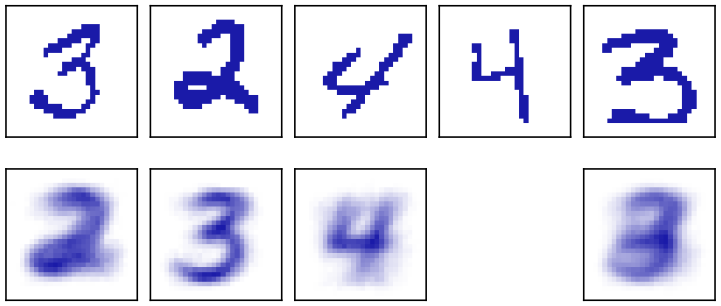
fig9_10. Download: PDF · SVGPriors and more than two states p. 448. Conjugate Beta priors on the \(\mu_{ki}\) act like extra pseudo-observations (Section 2.1.1), and EM then maximises the posterior (Exercise 9.18). Variables with \(M\gt2\) states are handled with the discrete distribution (2.26) in place of the Bernoulli, optionally with Dirichlet priors (Exercise 9.19).
Filling the gap 9.13: MAP with Beta and Dirichlet priors, and the multinomial mixture p. 448; Exercises 9.18 and 9.19
The book only says these extensions are "straightforward". Here are both M steps, with the conditions under which they are maxima.
Derivation
Beta and Dirichlet priors (Exercise 9.18). Let \(\mu_{ki}\sim\mathrm{Beta}(a_k,b_k)\) independently (2.13) and \(\bm\pi\sim\Dir(\bm\alpha)\) (2.38). By the MAP gap box the E step is (9.56) and the M step maximises (9.55) plus
\[ \ln p(\bm\mu,\bm\pi)=\sum_k(\alpha_k-1)\ln\pi_k+\sum_k\sum_i\big[(a_k-1)\ln\mu_{ki}+(b_k-1)\ln(1-\mu_{ki})\big]+\const . \]For \(\mu_{ki}\) the objective is \(A\ln\mu_{ki}+B\ln(1-\mu_{ki})\) with \(A=\sum_n\gamma_{nk}x_{ni}+a_k-1\) and \(B\)
With \(a_k,b_k\gt1\) this lies strictly inside \((0,1)\), so the zero-probability problem disappears; \(a_k=b_k=2\) is "add one to each count" (Laplace smoothing). For \(\bm\pi\), the objective \(\sum_k(N_k+\alpha_k-1)\ln\pi_k\) with Lagrange multiplier \(\lambda\): multiplying \((N_k+\alpha_k-1)/\pi_k+\lambda=0\) by \(\pi_k\) and summing over \(k\) gives \(\lambda=-(N+\hat\alpha-K)\) with \(\hat\alpha=\sum_k\alpha_k\), so
\[ \pi_k=\frac{N_k+\alpha_k-1}{N+\hat\alpha-K}, \]which is a global maximum by the Gibbs-inequality argument whenever all \(\alpha_k\ge1\) (the coefficients \(N_k+\alpha_k-1\) are then nonnegative). If some \(\alpha_k\lt1\) and \(N_k+\alpha_k-1\lt0\), the objective tends to \(+\infty\) as \(\pi_k\to0\) and there is no MAP estimate. With \(a_k=b_k=1\) and \(\bm\alpha=\mathbf{1}\) (flat priors) both updates reduce to (9.59)–(9.60).
Multinomial variables (Exercise 9.19). Now \(\mathbf{x}\) has \(D\) groups of \(M\) binary entries \(x_{ij}\) with \(\sum_jx_{ij}=1\) for each \(i\), and \(p(\mathbf{x}\given\bm\mu_k)\)
global maxima again by Gibbs' inequality. With Dirichlet priors \(\Dir(\bm\mu_{ki}\given\bm\beta_{ki})\) the same steps give
\[ \mu_{kij}=\frac{\sum_n\gamma_{nk}x_{nij}+\beta_{kij}-1}{N_k+\sum_j\beta_{kij}-M}. \]For \(M=2\) (with \(x_{i1}=x_i\), \(x_{i2}=1-x_i\)) everything reduces to the Bernoulli case. ∎
9.3.4 EM for Bayesian linear regression
pp. 448–450 The latent variable can also be continuous. In the evidence framework of Section 3.5, the hyperparameters \(\alpha\) (prior precision of the weights) and \(\beta\) (noise precision) are chosen to maximise the marginal likelihood \(p(\mathbf{t}\given\alpha,\beta)\)
and its posterior expectation is
\[ \E\big[\ln p(\mathbf{t},\mathbf{w}\given\alpha,\beta)\big]=\frac M2\ln\Big(\frac{\alpha}{2\pi}\Big)-\frac\alpha2\E\big[\mathbf{w}^\T\mathbf{w}\big]+\frac N2\ln\Big(\frac{\beta}{2\pi}\Big)-\frac\beta2\sum_{n=1}^{N}\E\big[(t_n-\mathbf{w}^\T\bm\phi_n)^2\big]. \tag{9.62} \]Filling the gap 9.14: the E step and the expectations in (9.62) pp. 448–449, (9.61)–(9.62)
We re-derive the posterior of Chapter 3 by completing the square and evaluate the two expectations that (9.62) leaves implicit.
Derivation
Posterior. As a function of \(\mathbf{w}\),
\[ \ln p(\mathbf{w}\given\mathbf{t})=-\frac\beta2\lVert\mathbf{t}-\bm\Phi\mathbf{w}\rVert^2-\frac\alpha2\mathbf{w}^\T\mathbf{w}+\const=-\frac12\mathbf{w}^\T(\alpha\mathbf{I}+\beta\bm\Phi^\T\bm\Phi)\mathbf{w}+\beta\mathbf{w}^\T\bm\Phi^\T\mathbf{t}+\const . \]By completing the square, this is \(\N(\mathbf{w}\given\mathbf{m}_N,\mathbf{S}_N)\) with \(\mathbf{S}_N^{-1}\)
(9.61)–(9.62). The two log densities are \(\ln p(\mathbf{t}\given\mathbf{w},\beta)\)
The expectations. Under \(\N(\mathbf{m}_N,\mathbf{S}_N)\), \(\E[\mathbf{w}\mathbf{w}^\T]\)
The scalar \(\mathbf{w}^\T\bm\phi_n\) has mean \(\mathbf{m}_N^\T\bm\phi_n\) and variance \(\bm\phi_n^\T\mathbf{S}_N\bm\phi_n\), so \(\E[(t_n-\mathbf{w}^\T\bm\phi_n)^2]\)
∎
Maximising (9.62) over \(\alpha\) gives (Exercise 9.20)
\[ \alpha=\frac{M}{\E[\mathbf{w}^\T\mathbf{w}]}=\frac{M}{\mathbf{m}_N^\T\mathbf{m}_N+\Tr(\mathbf{S}_N)}, \tag{9.63} \]and an analogous update holds for \(\beta\) (Exercise 9.21). This differs in form from the update \(\alpha\)
and at a stationary point of the evidence, where (3.92) holds,
\[ \alpha\,\mathbf{m}_N^\T\mathbf{m}_N=\gamma=M-\alpha\Tr(\mathbf{S}_N), \tag{9.65} \]which, solved for \(\alpha\), is (9.63).
Result 9.12 (EM for the evidence; Exercises 9.20 and 9.21) p. 449, (9.63)–(9.65)
With \(\mathbf{m}_N\), \(\mathbf{S}_N\) computed at the old \((\alpha,\beta)\), the M step is (9.63) together with
\[ \frac{1}{\beta^{\rm new}}=\frac1N\Big\{\lVert\mathbf{t}-\bm\Phi\mathbf{m}_N\rVert^2+\Tr(\bm\Phi^\T\bm\Phi\mathbf{S}_N)\Big\}. \]A pair \((\alpha,\beta)\) is a fixed point of these updates if and only if it satisfies the evidence re-estimation equations \(\alpha\)
Proof
M step. \(\partial(9.62)/\partial\alpha\)
Two trace identities. Let \(\beta\bm\Phi^\T\bm\Phi\mathbf{u}_i\)
The first is (9.64) (with (3.91)); the second holds because \(\beta\bm\Phi^\T\bm\Phi\mathbf{S}_N\) has eigenvalues \(\lambda_i/(\alpha+\lambda_i)\).
Fixed points. \(\alpha\)
Stationarity of the evidence. Equations (3.92) and (3.95) are rearrangements of \(\partial\ln p(\mathbf{t}\given\alpha,\beta)/\partial\alpha\)
The relevance vector machine pp. 449–450. In the RVM of Section 7.2.1 each weight has its own prior precision, \(p(\mathbf{w}\given\bm\alpha)\)
(the expectation under the posterior at the old hyperparameters; early printings lack the braces), giving
\[ \alpha_i^{\rm new}=\frac{1}{m_i^2+\Sigma_{ii}}, \tag{9.67} \] \[ (\beta^{\rm new})^{-1}=\frac{\lVert\mathbf{t}-\bm\Phi\mathbf{m}\rVert^2+\beta^{-1}\sum_i\gamma_i}{N}, \tag{9.68} \]with \(\gamma_i=1-\alpha_i\Sigma_{ii}\) (7.89). Erratum. Early printings have \(\mathbf{m}_N\) in (9.68); it is the RVM posterior mean \(\mathbf{m}\) of (7.82).
Result 9.13 (EM for the RVM; Exercises 9.22 and 9.23) p. 450, (9.66)–(9.68)
(a) Maximising (9.66) gives (9.67) and (9.68), where \(\beta^{-1}\) and the \(\gamma_i=1-\alpha_i\Sigma_{ii}\) on the right of (9.68) use the old hyperparameters. (b) At any fixed point, (9.67)–(9.68) are equivalent to the direct re-estimation equations \(\alpha_i=\gamma_i/m_i^2\) (7.87) and \((\beta)^{-1}\)
Proof
(a) As in the previous gap box, (9.66) equals, up to constants,
\[ \sum_i\Big[\frac12\ln\alpha_i-\frac{\alpha_i}{2}(m_i^2+\Sigma_{ii})\Big]+\frac N2\ln\beta-\frac\beta2\Big\{\lVert\mathbf{t}-\bm\Phi\mathbf{m}\rVert^2+\Tr(\bm\Phi^\T\bm\Phi\bm\Sigma)\Big\}, \]using \(\E[w_i^2]=m_i^2+\Sigma_{ii}\). Each \(\alpha_i\) appears in one concave term, \(\frac{1}{2\alpha_i}-\frac12(m_i^2+\Sigma_{ii})\)
(b) At a fixed point old and new values coincide. Then \(\alpha_i(m_i^2+\Sigma_{ii})\)
9.4 The EM algorithm in general
pp. 450–455 We now prove that EM works, for any model with observed variables \(\mathbf{X}\), hidden variables \(\mathbf{Z}\) and a joint distribution \(p(\mathbf{X},\mathbf{Z}\given\bm\theta)\) (Dempster et al., 1977; the view below is that of Csiszár and Tusnády, 1984, Hathaway, 1986, and Neal and Hinton, 1998). The goal is to maximise
\[ p(\mathbf{X}\given\bm\theta)=\sum_{\mathbf{Z}}p(\mathbf{X},\mathbf{Z}\given\bm\theta), \tag{9.69} \]assuming that \(p(\mathbf{X},\mathbf{Z}\given\bm\theta)\) is much easier to work with. For discrete \(\mathbf{Z}\) we write sums; for continuous or mixed \(\mathbf{Z}\) replace them by integrals. For any distribution \(q(\mathbf{Z})\) over the latent variables,
\[ \ln p(\mathbf{X}\given\bm\theta)=\LB(q,\bm\theta)+\KL(q\|p), \tag{9.70} \] \[ \LB(q,\bm\theta)=\sum_{\mathbf{Z}}q(\mathbf{Z})\ln\Big\{\frac{p(\mathbf{X},\mathbf{Z}\given\bm\theta)}{q(\mathbf{Z})}\Big\}, \tag{9.71} \] \[ \KL(q\|p)=-\sum_{\mathbf{Z}}q(\mathbf{Z})\ln\Big\{\frac{p(\mathbf{Z}\given\mathbf{X},\bm\theta)}{q(\mathbf{Z})}\Big\}. \tag{9.72} \]\(\LB(q,\bm\theta)\) is a functional of the distribution \(q\) (Appendix D) and a function of \(\bm\theta\). Note the differences between (9.71) and (9.72): opposite signs, and the joint distribution in \(\LB\) against the posterior in \(\KL\).
Result 9.14 (the decomposition; Exercise 9.24) pp. 450–451, (9.70)–(9.73)
Let \(p(\mathbf{X}\given\bm\theta)\gt0\) and let \(q\) be a distribution with \(q(\mathbf{Z})=0\) wherever \(p(\mathbf{Z}\given\mathbf{X},\bm\theta)\)
Proof
Line 1 (product rule). For every \(\mathbf{Z}\) with \(p(\mathbf{X},\mathbf{Z}\given\bm\theta)\)
Line 2 (divide by \(q\)). Let \(\mathbf{Z}\) have \(q(\mathbf{Z})\gt0\); by assumption its posterior, hence its joint probability, is positive. Subtracting \(\ln q(\mathbf{Z})\) from both sides of (9.73):
\[ \ln\frac{p(\mathbf{X},\mathbf{Z}\given\bm\theta)}{q(\mathbf{Z})}=\ln\frac{p(\mathbf{Z}\given\mathbf{X},\bm\theta)}{q(\mathbf{Z})}+\ln p(\mathbf{X}\given\bm\theta). \]Line 3 (average over \(q\)). Multiply by \(q(\mathbf{Z})\) and sum over the \(\mathbf{Z}\) with \(q(\mathbf{Z})\gt0\) (the others contribute nothing to (9.71) or (9.72), with \(0\ln0=0\)). The left side becomes \(\LB(q,\bm\theta)\), the first term on the right becomes \(-\KL(q\|p)\), and the last becomes \(\ln p(\mathbf{X}\given\bm\theta)\sum_{\mathbf{Z}}q(\mathbf{Z})\)
Line 4 (sign of KL). By Gibbs' inequality (KL divergence, Section 1.6.1), using \(\ln t\le t-1\) with equality only at \(t=1\): \(-\KL(q\|p)\)
(If \(q\) puts mass where the posterior is zero, then \(\KL=+\infty\) and \(\LB=-\infty\), and (9.70) still holds in the extended sense. For mixtures with all \(\pi_k\gt0\) the posterior is positive everywhere and the condition is empty.) ∎
The two steps as coordinate ascent on \(\LB\). pp. 451–452 In the E step, \(\LB(q,\bm\theta^{\rm old})\) is maximised over \(q\) with \(\bm\theta^{\rm old}\) fixed. Since \(\ln p(\mathbf{X}\given\bm\theta^{\rm old})\) does not depend on \(q\), (9.70) says that maximising \(\LB\) is minimising the KL term, so the unique maximiser is the posterior \(q(\mathbf{Z})\)
so the M step of Section 9.3 is exactly the maximisation of the bound.
Filling the gap 9.15: the bound is \(Q\) plus an entropy p. 452, (9.74)
One line of algebra, plus a word on the constant, which the book calls the entropy of \(q\) (early printings say "negative entropy"; the errata delete "negative").
Derivation
Split the logarithm in (9.71): \(\ln\{p(\mathbf{X},\mathbf{Z}\given\bm\theta)/q(\mathbf{Z})\}\)
\(\mathrm{H}[q]\) is the entropy of \(q\) (nonnegative for a discrete \(\mathbf{Z}\)) and does not involve \(\bm\theta\). The parameter appears only inside \(\ln p(\mathbf{X},\mathbf{Z}\given\bm\theta)\), so when the joint distribution is an exponential family the logarithm cancels the exponential and the M step is a complete-data maximum likelihood problem with expected sufficient statistics (Result 9.6). ∎
Result 9.15 (EM never decreases the log likelihood) pp. 451–454
Let \(q\)
The log likelihood stays the same only if \(\bm\theta^{\rm old}\) also maximises \(Q(\cdot,\bm\theta^{\rm old})\) and the posterior over \(\mathbf{Z}\) is unchanged.
Proof
Apply (9.70) at \(\bm\theta^{\rm new}\) with this \(q\), then (9.74):
\[ \ln p(\mathbf{X}\given\bm\theta^{\rm new})=\LB(q,\bm\theta^{\rm new})+\KL\big(q\|p(\cdot\given\mathbf{X},\bm\theta^{\rm new})\big)=Q(\bm\theta^{\rm new},\bm\theta^{\rm old})+\mathrm{H}[q]+\KL\big(q\|p(\cdot\given\mathbf{X},\bm\theta^{\rm new})\big). \]At \(\bm\theta^{\rm old}\) the KL term is zero (E step), so \(\ln p(\mathbf{X}\given\bm\theta^{\rm old})\)
What monotonicity does and does not give. The sequence \(\ln p(\mathbf{X}\given\bm\theta^{(t)})\) is nondecreasing, so it converges whenever the likelihood is bounded above (Bernoulli mixtures; Gaussian mixtures with a variance floor or a Wishart prior), and otherwise it may run off to \(+\infty\) along a singularity (Figure 9.7): monotonicity drives EM into a collapse rather than protecting against it. It does not by itself imply that the parameters converge, or that their limit is a maximum. Under mild regularity conditions (for example, \(Q\) continuous in both arguments and the set \(\{\bm\theta:\ln p(\mathbf{X}\given\bm\theta)\)
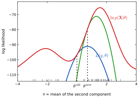
fig9_14. Download: PDF · SVGShape of the bound. p. 453 The book says the bound is "a convex function having a unique maximum"; erratum: it should read concave. For exponential-family components, \(Q(\bm\eta,\bm\eta^{\rm old})\) is concave in the natural parameters by Result 9.6 (for instance \(N_1\ln\pi+N_2\ln(1-\pi)\) for a mixing weight, or a downward parabola for a mean), which is what the figure shows. The bound also touches the log likelihood tangentially:
Result 9.16 (the bound is tangent to the log likelihood; Exercise 9.25) p. 453
Let \(q^{\rm old}\)
Consequently, every fixed point \(\bm\theta^\star\) of EM in the interior of the parameter space (a point that maximises \(Q(\cdot,\bm\theta^\star)\)) is a stationary point of \(\ln p(\mathbf{X}\given\bm\theta)\); conversely, a stationary point of the log likelihood is a stationary point of \(Q(\cdot,\bm\theta^\star)\), hence a fixed point of EM whenever \(Q(\cdot,\bm\theta^\star)\) has a unique stationary point (e.g. is strictly concave).
Proof
First proof (the KL term is minimal). By (9.70), \(\LB(q^{\rm old},\bm\theta)\)
Second proof (Fisher's identity). \(\nabla_{\bm\theta}\LB(q^{\rm old},\bm\theta)\)
i.e. the observed-data score is the posterior mean of the complete-data score.
Fixed points. If \(\bm\theta^\star\) maximises \(Q(\cdot,\bm\theta^\star)\) at an interior point, then \(\nabla_{\bm\theta}Q(\bm\theta,\bm\theta^\star)\)
Going further: how fast does EM converge?
The book notes that EM needs many more iterations than K-means. Near a maximum, EM converges linearly, at a rate set by the proportion of information that the latent variables hide (Dempster et al., 1977).
Result 9.17 (going further: the rate of convergence of EM)
Suppose EM converges to an interior strict local maximiser \(\bm\theta^\star\) of \(\ln p(\mathbf{X}\given\bm\theta)\), that the EM map \(M(\bm\theta')\)
the last expectation under \(p(\mathbf{Z}\given\mathbf{X},\bm\theta^\star)\), with \(\mathbf{I}_{\rm obs}\) and \(\mathbf{I}_{\rm c}\) positive definite. Then \(\mathbf{I}_{\rm c}\)
The eigenvalues of \(\mathbf{J}\) lie in \([0,1)\); the largest, the largest fraction of missing information, is the linear rate. It approaches 1, and EM crawls, when the latent variables carry most of the information, as when components overlap.
Proof
Jacobian of the EM map. Let \(\mathbf{g}(\bm\theta,\bm\theta')\)
The cross derivative. \(g_i(\bm\theta,\bm\theta')\)
using \(\ln p(\mathbf{X},\mathbf{Z})\)
Missing information principle. For every \(\mathbf{Z}\), \(\ln p(\mathbf{X}\given\bm\theta)\)
Eigenvalues. \(\mathbf{J}\) is similar to \(\mathbf{I}_{\rm c}^{-1/2}\mathbf{I}_{\rm mis}\mathbf{I}_{\rm c}^{-1/2}\), which is symmetric positive semidefinite, so its eigenvalues are real and \(\ge0\); and \(\mathbf{I}-\mathbf{J}\) is similar to \(\mathbf{I}_{\rm c}^{-1/2}\mathbf{I}_{\rm obs}\mathbf{I}_{\rm c}^{-1/2}\), positive definite, so they are \(\lt1\). Finally \(\bm\theta^{(t+1)}-\bm\theta^\star\)
A numerical illustration (seeded, our own run): 300 points, half from \(\N(0,1)\) and half from \(\N(s,1)\), fitted by a two-component mixture with unit variances and free \((\pi,\mu_1,\mu_2)\). The largest eigenvalue of \(\mathbf{J}\) is 0.25 for \(s=4\) (19 iterations to reach a tolerance of \(10^{-13}\)), 0.89 for \(s=2\) (224 iterations) and 0.97 for \(s=1.2\) (863 iterations); a finite-difference Jacobian of the actual EM map agrees with \(\mathbf{I}-\mathbf{I}_{\rm c}^{-1}\mathbf{I}_{\rm obs}\) to about \(3\times10^{-6}\). Newton-type methods converge faster near a maximum but give up EM's monotonicity and simplicity.
Independent observations. p. 453 For an i.i.d. data set, \(\mathbf{X}=\{\mathbf{x}_n\}\), \(\mathbf{Z}=\{\mathbf{z}_n\}\) and \(p(\mathbf{X},\mathbf{Z})\)
so the responsibility of a component for \(\mathbf{x}_n\) depends only on \(\mathbf{x}_n\) and \(\bm\theta\), not on the other data points.
Filling the gap 9.16: the last equality in (9.75) p. 453, (9.75)
The book says "using the sum and product rules". The key step is that a sum over all \(\mathbf{Z}\) of a product of factors, each depending on one \(\mathbf{z}_n\), is the product of the separate sums.
Derivation
A sum over \(\mathbf{Z}\) is a sum over \(\mathbf{z}_1,\dots,\mathbf{z}_N\) independently, so by the distributive law
\[ \sum_{\mathbf{Z}}\prod_{n=1}^{N}p(\mathbf{x}_n,\mathbf{z}_n\given\bm\theta)=\sum_{\mathbf{z}_1}\cdots\sum_{\mathbf{z}_N}\prod_{n}p(\mathbf{x}_n,\mathbf{z}_n\given\bm\theta)=\prod_{n=1}^{N}\sum_{\mathbf{z}_n}p(\mathbf{x}_n,\mathbf{z}_n\given\bm\theta)=\prod_{n=1}^{N}p(\mathbf{x}_n\given\bm\theta). \](For \(N=2\): \(\sum_{a}\sum_{b}f(a)g(b)\)
MAP estimation. p. 454 For a prior \(p(\bm\theta)\), \(p(\bm\theta\given\mathbf{X})\)
and with the decomposition (9.70),
\[ \begin{aligned}\ln p(\bm\theta\given\mathbf{X})&=\LB(q,\bm\theta)+\KL(q\|p)+\ln p(\bm\theta)-\ln p(\mathbf{X})\\&\ge\LB(q,\bm\theta)+\ln p(\bm\theta)-\ln p(\mathbf{X}),\end{aligned} \tag{9.77} \]where \(\ln p(\mathbf{X})\) is a constant.
Filling the gap 9.17: MAP-EM increases the posterior p. 454, (9.76)–(9.77)
The book says that the right-hand side of (9.77) can be optimised alternately over \(q\) and \(\bm\theta\). Here is why the E step is unchanged and why the posterior cannot decrease.
Derivation
(9.76) is the logarithm of the product rule \(p(\bm\theta,\mathbf{X})\)
E step. In the right-hand side of (9.77), only \(\LB(q,\bm\theta)\) depends on \(q\), so the maximising \(q\) is again \(p(\mathbf{Z}\given\mathbf{X},\bm\theta^{\rm old})\), and then (9.77) holds with equality at \(\bm\theta^{\rm old}\).
M step and monotonicity. With that \(q\) fixed, maximise \(\LB(q,\bm\theta)+\ln p(\bm\theta)\)
For conjugate priors the change to the M step is small: the prior adds pseudo-counts to the expected sufficient statistics (see the Wishart and Dirichlet examples in Section 9.3 and the Beta example in Section 9.3.3). ∎
Generalised EM and ECM
p. 454 If the M step cannot be carried out exactly, Result 9.15 still applies to any \(\bm\theta^{\rm new}\) with \(Q(\bm\theta^{\rm new},\bm\theta^{\rm old})\)
Partial E steps
pp. 454–455 The E step can be generalised in the same way: any change of \(q\) that increases \(\LB(q,\bm\theta)\) is allowed (Neal and Hinton, 1998). EM is then plain coordinate ascent on the single function \(\LB(q,\bm\theta)\), and maxima of \(\LB\) correspond to maxima of the likelihood.
Result 9.18 (maxima of the bound are maxima of the likelihood) pp. 454–455
(a) For every \(\bm\theta\), \(\max_q\LB(q,\bm\theta)\)
(b) If \(\bm\theta^\star\) is a local maximiser of \(\ln p(\mathbf{X}\given\bm\theta)\), then \((q_{\bm\theta^\star},\bm\theta^\star)\) is a local maximiser of \(\LB\). Conversely, if \((q^\star,\bm\theta^\star)\) is a local maximiser of \(\LB\) and the posterior \(q_{\bm\theta}\) depends continuously on \(\bm\theta\), then \(q^\star=q_{\bm\theta^\star}\) and \(\bm\theta^\star\) is a local maximiser of \(\ln p(\mathbf{X}\given\bm\theta)\).
Proof
(a) Result 9.14: \(\LB(q,\bm\theta)\)
(b) First part: for \((q,\bm\theta)\) near \((q_{\bm\theta^\star},\bm\theta^\star)\), \(\LB(q,\bm\theta)\)
So any algorithm that keeps increasing \(\LB\), by full or partial steps in \(q\) or \(\bm\theta\), is hunting for maxima of the likelihood. Chapter 10 keeps this objective but restricts \(q\) to a tractable family, which is variational inference.
Incremental EM
p. 455 For i.i.d. data, take \(q=\prod_nq_n(\mathbf{z}_n)\), so that \(\LB\) is a sum over points (see the gap box on (9.75)). Updating a single \(q_m\) to the posterior of point \(m\) is a partial E step, and it increases \(\LB\). For exponential-family components the following M step only needs sufficient statistics, which change by the contribution of one point. For a Gaussian mixture, writing \(\gamma^{\rm old}(z_{mk})\) and \(\gamma^{\rm new}(z_{mk})\) for the responsibilities of point \(m\) before and after its partial E step,
\[ \bm\mu_k^{\rm new}=\bm\mu_k^{\rm old}+\Big(\frac{\gamma^{\rm new}(z_{mk})-\gamma^{\rm old}(z_{mk})}{N_k^{\rm new}}\Big)\big(\mathbf{x}_m-\bm\mu_k^{\rm old}\big), \tag{9.78} \] \[ N_k^{\rm new}=N_k^{\rm old}+\gamma^{\rm new}(z_{mk})-\gamma^{\rm old}(z_{mk}). \tag{9.79} \]Result 9.19 (incremental updates of all the sufficient statistics; Exercises 9.26 and 9.27) p. 455, (9.78)–(9.79)
Let \(\Delta_k\)
provided \(N_k^{\rm new}\gt0\). (The matrix \((\mathbf{x}_m-\bm\mu_k^{\rm new})(\mathbf{x}_m-\bm\mu_k^{\rm old})^\T\) is symmetric, being \(\frac{N_k^{\rm old}}{N_k^{\rm new}}(\mathbf{x}_m-\bm\mu_k^{\rm old})(\mathbf{x}_m-\bm\mu_k^{\rm old})^\T\).) Each update costs \(O(KD^2)\), independently of \(N\).
Proof
Write \(N=N_k^{\rm old}\), \(N'=N_k^{\rm new}\), \(\bm\mu=\bm\mu_k^{\rm old}\), \(\bm\mu'=\bm\mu_k^{\rm new}\), \(\mathbf{x}=\mathbf{x}_m\), \(\Delta=\Delta_k\) (for this proof only, \(N\) is the effective count of component \(k\)).
Counts (9.79). \(N_k=\sum_n\gamma(z_{nk})\) and only the term \(n=m\) changes, by \(\Delta\).
Means (9.78), Exercise 9.26. \(N'\bm\mu'\)
Covariances, Exercise 9.27. Expanding (9.25) with \(\mathbf{W}_k\)
Divide by \(N'\) and write \(N/N'=1-\Delta/N'\): \(\bm\Sigma'\)
Mixing coefficients. \(\pi_k=N_k/N_{\rm tot}\) with the total \(N_{\rm tot}=\sum_kN_k=N\) unchanged, because both the old and the new responsibilities of point \(m\) sum to one over \(k\), i.e. \(\sum_k\Delta_k=0\). So \(\pi_k\) changes by \(\Delta_k/N\) and still sums to one.
Cost. Each update is a few vector and outer-product operations per component, \(O(KD^2)\); \(\bm\Sigma_k\) changes by a scaling plus a rank-one term, so its Cholesky factor can be updated in \(O(D^2)\) rather than recomputed. ∎
Algorithm 9.6 (incremental EM for a Gaussian mixture; Neal and Hinton, 1998)
- Initialise the parameters, do one full E step and store all responsibilities; compute \(N_k\), \(\bm\mu_k\), \(\bm\Sigma_k\), \(\pi_k\) by (9.24)–(9.27).
- For \(m=1,2,\dots\) (cycling through the data, possibly in random order):
- Partial E step: recompute the responsibilities of point \(m\) only, (9.23).
- M step: update \(N_k\), \(\bm\mu_k\), \(\bm\Sigma_k\), \(\pi_k\) by Result 9.19, and store the new responsibilities of point \(m\).
- Stop when a full sweep through the data changes the parameters (or \(\LB\)) by less than a tolerance.
Each step increases \(\LB(q,\bm\theta)\) with \(q=\prod_nq_n\) the stored responsibilities, so by Result 9.18 the algorithm is looking for local maxima of the likelihood. Note that it is \(\LB\), not \(\ln p(\mathbf{X}\given\bm\theta)\), that increases at every step: between full sweeps \(q\) is not the exact posterior, so \(\ln p(\mathbf{X}\given\bm\theta^{(t)})\)
Exercises
All 27 exercises of Chapter 9 (Bishop, 2006, pp. 455–459), restated in my own words, with complete solutions (hidden). Stars give the book's difficulty and "www" marks the exercises with official solutions. Several solutions are compact versions of the gap boxes and results above, which are linked for more detail.
Exercise 9.1 (★, www). Using that there are finitely many possible assignments \(\{r_{nk}\}\), and that each assignment has a unique optimal set of prototypes, show that K-means converges after a finite number of iterations.
Solution
Let \(F(r)=\min_{\bm\mu}J(r,\bm\mu)\); for nonempty clusters the minimiser is unique, the cluster means (gap box 9.1), and empty clusters contribute nothing to \(J\). After every M step, \(J=F(r^{(t)})\). Break ties in the E step in favour of the current cluster. If the E step changes the assignment, some point moves to a strictly nearer prototype, so \(J(r^{(t+1)},\bm\mu^{(t)})\)
\({}\lt J(r^{(t)},\bm\mu^{(t)})\) \({}=F(r^{(t)})\), and the M step cannot increase \(J\): \(F(r^{(t+1)})\lt F(r^{(t)})\). A strictly decreasing sequence of values of \(F\) cannot revisit an assignment, and there are at most \(K^N\) assignments, so after finitely many iterations the E step leaves the assignment unchanged; the M step then reproduces the same means, and the algorithm has converged. The limit is a configuration in which neither step can improve \(J\), not necessarily the global minimum (Result 9.1). ▶ See it in a demo: a K-means run that stops at a poor local minimum
Exercise 9.2 (★). Apply the Robbins–Monro procedure of Section 2.3.5 to find the roots of the derivatives of \(J\) with respect to the \(\bm\mu_k\), and show that it gives the sequential update (9.5) of the nearest prototype.
Solution
For data arriving from \(p(\mathbf{x})\), the per-point expected distortion \(\bar J(\bm\mu)\)
\({}=\E[\min_k\lVert\mathbf{x}-\bm\mu_k\rVert^2]\) has \(\nabla_{\bm\mu_k}\bar J\) \({}=\E[-2r_k(\mathbf{x};\bm\mu)(\mathbf{x}-\bm\mu_k)]\), where \(r_k(\mathbf{x};\bm\mu)=1\) if \(\bm\mu_k\) is the prototype nearest to \(\mathbf{x}\) (the integrand is differentiable except on cell boundaries, a null set when \(p\) has a density and the prototypes are distinct). This is a regression function whose root we want, and \(\mathbf{z}\) \({}=-2r_k(\mathbf{x}_n;\bm\mu)(\mathbf{x}_n-\bm\mu_k)\) is an unbiased noisy observation of it. The Robbins–Monro step (2.129), \(\bm\mu_k\leftarrow\bm\mu_k-a_{n-1}\mathbf{z}\), is \(\bm\mu_k\leftarrow\bm\mu_k+2a_{n-1}r_k(\mathbf{x}_n;\bm\mu)(\mathbf{x}_n-\bm\mu_k)\): nothing moves except the nearest prototype, which moves by (9.5) with \(\eta_n=2a_{n-1}\). The step sizes must satisfy (2.130)–(2.132); the choice \(\eta=1/m_k\), with \(m_k\) the number of points assigned to prototype \(k\) so far, does, and makes \(\bm\mu_k\) the running mean of those points (MacQueen, 1967). Details in gap box 9.2. Exercise 9.3 (★, www). With \(p(\mathbf{z})\) given by (9.10) and \(p(\mathbf{x}\given\mathbf{z})\) by (9.11), show that summing \(p(\mathbf{z})p(\mathbf{x}\given\mathbf{z})\) over the values of \(\mathbf{z}\) gives the Gaussian mixture (9.7).
Solution
\(p(\mathbf{z})p(\mathbf{x}\given\mathbf{z})\)
\({}=\prod_k\{\pi_k\N(\mathbf{x}\given\bm\mu_k,\bm\Sigma_k)\}^{z_k}\). The variable \(\mathbf{z}\) takes the \(K\) values \(\mathbf{e}_j\), and for \(\mathbf{z}=\mathbf{e}_j\) every factor with \(k\ne j\) is raised to the power 0, so the product equals \(\pi_j\N(\mathbf{x}\given\bm\mu_j,\bm\Sigma_j)\). Summing over \(j\) gives \(\sum_j\pi_j\N(\mathbf{x}\given\bm\mu_j,\bm\Sigma_j)\), which is (9.7). Exercise 9.4 (★). To maximise the posterior \(p(\bm\theta\given\mathbf{X})\) of a latent-variable model by EM, show that the E step is as for maximum likelihood and that the M step maximises \(Q(\bm\theta,\bm\theta^{\rm old})+\ln p(\bm\theta)\).
Solution
\(\ln p(\bm\theta\given\mathbf{X})\)
\({}=\ln p(\mathbf{X}\given\bm\theta)+\ln p(\bm\theta)-\ln p(\mathbf{X})\), and the last term is constant. With \(q(\mathbf{Z})\) \({}=p(\mathbf{Z}\given\mathbf{X},\bm\theta^{\rm old})\), Jensen's inequality gives \(\ln p(\mathbf{X}\given\bm\theta)\) \({}\ge Q(\bm\theta,\bm\theta^{\rm old})+\mathrm{H}[q]\) with equality at \(\bm\theta^{\rm old}\) (gap box 9.8). Adding \(\ln p(\bm\theta)\): the function \(Q(\bm\theta,\bm\theta^{\rm old})+\ln p(\bm\theta)+\mathrm{H}[q]\) is a lower bound on \(\ln p(\mathbf{X}\given\bm\theta)+\ln p(\bm\theta)\) that touches it at \(\bm\theta^{\rm old}\), so any \(\bm\theta\) that increases \(Q+\ln p(\bm\theta)\) increases the log posterior. The E step, the computation of \(q\), involves only the posterior of \(\mathbf{Z}\) at \(\bm\theta^{\rm old}\), in which the prior plays no role, so it is unchanged; the M step maximises \(Q(\bm\theta,\bm\theta^{\rm old})+\ln p(\bm\theta)\). (Equivalently, in the language of Section 9.4: maximise the right-hand side of (9.77) alternately over \(q\) and \(\bm\theta\); see gap box 9.17.) Exercise 9.5 (★). Using d-separation in the graph of Figure 9.6, show that the posterior of the latent variables factorises over data points, \(p(\mathbf{Z}\given\mathbf{X},\bm\mu,\bm\Sigma,\bm\pi)\)
\({}=\prod_{n=1}^{N}p(\mathbf{z}_n\given\mathbf{x}_n,\bm\mu,\bm\Sigma,\bm\pi)\) (9.80). Solution
Condition on the observed \(\mathbf{x}_1,\dots,\mathbf{x}_N\) and on the parameters \(\bm\pi,\bm\mu,\bm\Sigma\). Any path from \(\mathbf{z}_n\) to \(\mathbf{z}_m\) (\(m\ne n\)) must leave the plate copy \(n\) through a parameter node: either \(\mathbf{z}_n\leftarrow\bm\pi\)
\({}\to\mathbf{z}_m\), or \(\mathbf{z}_n\) \({}\to\mathbf{x}_n\leftarrow\bm\mu\) \({}\to\mathbf{x}_m\leftarrow\mathbf{z}_m\) (or the same with \(\bm\Sigma\)). In each case the parameter node is tail to tail and conditioned on, which blocks the path (the head-to-head nodes \(\mathbf{x}_n\), \(\mathbf{x}_m\) are observed and would let the path through, but one blocked node suffices). So all \(\mathbf{z}_n\) are mutually independent given \(\mathbf{X}\) and the parameters, and since \(\mathbf{z}_n\) is independent of \(\mathbf{x}_m\) (\(m\ne n\)) given \(\mathbf{x}_n\) and the parameters by the same argument, each factor is \(p(\mathbf{z}_n\given\mathbf{x}_n,\bm\theta)\). Algebraically: \(p(\mathbf{Z}\given\mathbf{X})\) \({}=\prod_np(\mathbf{x}_n,\mathbf{z}_n)/\prod_np(\mathbf{x}_n)\) (Result 9.7). Exercise 9.6 (★★). Derive the EM algorithm for a Gaussian mixture in which all components share one covariance matrix \(\bm\Sigma\).
Solution
E step: (9.23) with every \(\bm\Sigma_k=\bm\Sigma\). M step: with \(\bm\Lambda=\bm\Sigma^{-1}\) the expected complete-data log likelihood is
\[ \sum_{n,k}\gamma_{nk}\Big\{\ln\pi_k+\frac12\ln|\bm\Lambda|-\frac12(\mathbf{x}_n-\bm\mu_k)^\T\bm\Lambda(\mathbf{x}_n-\bm\mu_k)\Big\}+\const . \]For fixed \(\bm\Lambda\) it is strictly concave in each \(\bm\mu_k\) with maximiser \(\bm\mu_k\)
\[ \bm\Sigma=\frac1N\sum_{k=1}^{K}\sum_{n=1}^{N}\gamma_{nk}(\mathbf{x}_n-\bm\mu_k)(\mathbf{x}_n-\bm\mu_k)^\T=\sum_{k=1}^{K}\pi_k\,\bm\Sigma_k^{\rm sep}, \]\({}=N_k^{-1}\sum_n\gamma_{nk}\mathbf{x}_n\), independent of \(\bm\Lambda\) (as in Result 9.8); \(\pi_k=N_k/N\) as before. With these means, and \(\sum_kN_k=N\), the \(\bm\Lambda\)-terms are \(\frac N2\ln|\bm\Lambda|-\frac12\Tr\big(\bm\Lambda\sum_k\widetilde{\mathbf{S}}_k\big)\), with \(\widetilde{\mathbf{S}}_k\) \({}=\sum_n\gamma_{nk}(\mathbf{x}_n-\bm\mu_k)(\mathbf{x}_n-\bm\mu_k)^\T\). The differential calculation of gap box 9.6 gives where \(\bm\Sigma_k^{\rm sep}\)
\({}=\widetilde{\mathbf{S}}_k/N_k\) is what (9.25) would give for component \(k\) alone: the shared covariance is the \(\pi\)-weighted average of the separate ones (the pooled within-component covariance). Because \(\bm\Sigma\) is estimated from all \(N\) points, it is nonsingular as soon as the data span \(\R^D\) around the means, so a single component can no longer collapse onto one point. Exercise 9.7 (★, www). Show that maximising the complete-data log likelihood (9.36) fits each component's mean and covariance to its own group of points, and sets the mixing coefficients to the fractions of points in the groups.
Solution
With \(\mathcal{C}_k=\{n:z_{nk}=1\}\) and \(N_k=|\mathcal{C}_k|\), (9.36) equals \(\sum_kN_k\ln\pi_k+\sum_k\sum_{n\in\mathcal{C}_k}\ln\N(\mathbf{x}_n\given\bm\mu_k,\bm\Sigma_k)\). Each \((\bm\mu_k,\bm\Sigma_k)\) appears only in the \(k\)th inner sum, the single-Gaussian log likelihood of group \(k\), maximised by the group mean and the group covariance with divisor \(N_k\) (2.121)–(2.122). For \(\bm\pi\), the Lagrangian \(\sum_kN_k\ln\pi_k+\lambda(\sum_k\pi_k-1)\) gives \(N_k/\pi_k+\lambda=0\); multiplying by \(\pi_k\) and summing over \(k\) gives \(\lambda=-N\) and \(\pi_k=N_k/N\), which is (9.37) and a global maximum by Gibbs' inequality (gap box 9.11).
Exercise 9.8 (★, www). Show that maximising (9.40) over \(\bm\mu_k\) with the responsibilities fixed gives (9.17).
Solution
By (2.43), the \(\bm\mu_k\)-dependent part of (9.40) is \(-\frac12\sum_n\gamma_{nk}(\mathbf{x}_n-\bm\mu_k)^\T\bm\Sigma_k^{-1}(\mathbf{x}_n-\bm\mu_k)\). Its gradient is \(\bm\Sigma_k^{-1}\sum_n\gamma_{nk}(\mathbf{x}_n-\bm\mu_k)\), which vanishes if and only if \(\bm\mu_k\)
\({}=N_k^{-1}\sum_n\gamma_{nk}\mathbf{x}_n\), i.e. (9.17). The Hessian \(-N_k\bm\Sigma_k^{-1}\) is negative definite (for \(N_k\gt0\)), so this is the unique maximum. Exercise 9.9 (★). Show that maximising (9.40) over \(\bm\Sigma_k\) and \(\pi_k\) with the responsibilities fixed gives (9.19) and (9.22).
Solution
With \(\bm\Lambda_k=\bm\Sigma_k^{-1}\) and the trace trick, the \(\bm\Lambda_k\)-terms of (9.40) are \(\frac{N_k}{2}\ln|\bm\Lambda_k|-\frac12\Tr(\bm\Lambda_k\widetilde{\mathbf{S}}_k)\) with \(\widetilde{\mathbf{S}}_k\)
\({}=\sum_n\gamma_{nk}(\mathbf{x}_n-\bm\mu_k)(\mathbf{x}_n-\bm\mu_k)^\T\). For a symmetric perturbation, its differential is \(\frac12\Tr\{(N_k\bm\Lambda_k^{-1}-\widetilde{\mathbf{S}}_k)\d\bm\Lambda_k\}\); the matrix in braces is symmetric, so the differential vanishes for all symmetric \(\d\bm\Lambda_k\) if and only if \(\bm\Sigma_k\) \({}=\widetilde{\mathbf{S}}_k/N_k\), which is (9.19). The function is strictly concave in \(\bm\Lambda_k\), so this is the maximum (Result 9.8). For \(\pi_k\), the \(\bm\pi\)-terms are \(\sum_kN_k\ln\pi_k\); the Lagrange argument with \(\sum_k\pi_k=1\) gives \(\lambda=-N\) and \(\pi_k=N_k/N\), which is (9.22) (gap box 9.7). Exercise 9.10 (★★). For a mixture \(p(\mathbf{x})\)
\({}=\sum_k\pi_kp(\mathbf{x}\given k)\) (9.81) and a partition \(\mathbf{x}\) \({}=(\mathbf{x}_a,\mathbf{x}_b)\), show that \(p(\mathbf{x}_b\given\mathbf{x}_a)\) is again a mixture, and find its mixing coefficients and components. Solution
The marginal is \(p(\mathbf{x}_a)\)
\[ p(\mathbf{x}_b\given\mathbf{x}_a)=\frac{\sum_k\pi_kp(\mathbf{x}_a,\mathbf{x}_b\given k)}{p(\mathbf{x}_a)}=\sum_{k=1}^{K}\underbrace{\frac{\pi_k\,p(\mathbf{x}_a\given k)}{\sum_j\pi_j\,p(\mathbf{x}_a\given j)}}_{w_k(\mathbf{x}_a)}\ p(\mathbf{x}_b\given\mathbf{x}_a,k), \]\({}=\sum_j\pi_jp(\mathbf{x}_a\given j)\), with \(p(\mathbf{x}_a\given j)\) the marginal of component \(j\). Then writing \(p(\mathbf{x}_a,\mathbf{x}_b\given k)\)
\[ p(\mathbf{x}_b\given\mathbf{x}_a,k)=\N\big(\mathbf{x}_b\given\bm\mu_{k,b}+\bm\Sigma_{k,ba}\bm\Sigma_{k,aa}^{-1}(\mathbf{x}_a-\bm\mu_{k,a}),\ \bm\Sigma_{k,bb}-\bm\Sigma_{k,ba}\bm\Sigma_{k,aa}^{-1}\bm\Sigma_{k,ab}\big): \]\({}=p(\mathbf{x}_a\given k)\,p(\mathbf{x}_b\given\mathbf{x}_a,k)\). The new mixing coefficients \(w_k(\mathbf{x}_a)\) are the responsibilities of the components for the observed part \(\mathbf{x}_a\); they are nonnegative and sum to one, and they depend on \(\mathbf{x}_a\). The components are the conditionals of the original components. For Gaussian components (partitioned Gaussians), \(p(\mathbf{x}_a\given k)\) \({}=\N(\mathbf{x}_a\given\bm\mu_{k,a},\bm\Sigma_{k,aa})\) and a mixture of linear-Gaussian regressions with input-dependent weights, as in the mixtures of experts of Section 14.5.
Exercise 9.11 (★). For the mixture with covariances \(\epsilon\mathbf{I}\) of Section 9.3.2, show that as \(\epsilon\to0\) maximising the expected complete-data log likelihood (9.40) is equivalent to minimising the distortion \(J\) of (9.1).
Solution
By (9.40)–(9.41),
\[ \E_{\mathbf{Z}}[\ln p]=\sum_{n,k}\gamma_{nk}\ln\pi_k-\frac{ND}{2}\ln(2\pi\epsilon)-\frac{1}{2\epsilon}\sum_{n,k}\gamma_{nk}\lVert\mathbf{x}_n-\bm\mu_k\rVert^2 . \]The middle term does not involve the parameters. As \(\epsilon\to0\), each \(\gamma_{nk}\to r_{nk}\) of (9.2) (for points with a unique nearest centre, at rate \(e^{-\Delta_n/2\epsilon}\), and assuming all \(\pi_k\gt0\)). Multiplying by \(\epsilon\gt0\) does not change the maximiser, and \(\epsilon\,\E_{\mathbf{Z}}[\ln p]\)
\({}\to-\frac12\sum_{n,k}r_{nk}\lVert\mathbf{x}_n-\bm\mu_k\rVert^2\) \({}=-\frac12J\), uniformly over bounded sets of means (the \(\ln\pi_k\) term is bounded and \(\epsilon\ln\epsilon\to0\)). Hence maximising over the means becomes minimising \(J\), and the maximiser itself, the weighted mean (9.17), converges to the K-means update (9.4). Full details in Result 9.9. ▶ See it in a demo: EM with shared covariance \(\epsilon\mathbf{I}\) turning into K-means
Exercise 9.12 (★, www). For a mixture (9.82) whose components (discrete, continuous or mixed) have means \(\bm\mu_k\) and covariances \(\bm\Sigma_k\), show that the mixture's mean and covariance are (9.49) and (9.50).
Solution
For any function \(f\), \(\E[f(\mathbf{x})]\)
\({}=\sum_k\pi_k\E_k[f(\mathbf{x})]\) by linearity of the sum or integral. With \(f(\mathbf{x})=\mathbf{x}\): \(\E[\mathbf{x}]=\sum_k\pi_k\bm\mu_k\), (9.49). With \(f(\mathbf{x})\) \({}=\mathbf{x}\mathbf{x}^\T\) and \(\E_k[\mathbf{x}\mathbf{x}^\T]\) \({}=\bm\Sigma_k+\bm\mu_k\bm\mu_k^\T\): \(\E[\mathbf{x}\mathbf{x}^\T]\) \({}=\sum_k\pi_k(\bm\Sigma_k+\bm\mu_k\bm\mu_k^\T)\), and \(\cov[\mathbf{x}]\) \({}=\E[\mathbf{x}\mathbf{x}^\T]-\E[\mathbf{x}]\E[\mathbf{x}]^\T\) gives (9.50). Equivalently \(\cov[\mathbf{x}]\) \({}=\sum_k\pi_k\bm\Sigma_k+\sum_k\pi_k(\bm\mu_k-\bar{\bm\mu})(\bm\mu_k-\bar{\bm\mu})^\T\) (Result 9.10). Exercise 9.13 (★★). Show that a Bernoulli mixture whose parameters are at a maximum of the likelihood satisfies \(\E[\mathbf{x}]\)
\({}=\frac1N\sum_n\mathbf{x}_n\equiv\bar{\mathbf{x}}\) (9.83). Show also that if all components start with the same mean \(\bm\mu_k=\widehat{\bm\mu}\), EM converges after one iteration, for any initial mixing coefficients, to \(\bm\mu_k=\bar{\mathbf{x}}\). Solution
First part. At an interior maximum the likelihood is stationary, so by the argument of Result 9.5 (with the Bernoulli derivatives of gap box 9.12) the parameters satisfy \(\bm\mu_k=\bar{\mathbf{x}}_k\) and \(\pi_k=N_k/N\) with the responsibilities evaluated at the maximum. Then
\[ \E[\mathbf{x}]=\sum_k\pi_k\bm\mu_k=\sum_k\frac{N_k}{N}\cdot\frac{1}{N_k}\sum_n\gamma_{nk}\mathbf{x}_n=\frac1N\sum_n\Big(\sum_k\gamma_{nk}\Big)\mathbf{x}_n=\bar{\mathbf{x}}, \]since \(\sum_k\gamma_{nk}=1\). (The same identity holds after every M step, maximum or not.)
Second part. If \(\bm\mu_k=\widehat{\bm\mu}\) for all \(k\), then \(p(\mathbf{x}_n\given\bm\mu_k)\) is the same for every \(k\), and (9.56) gives \(\gamma_{nk}=\pi_k\) for all \(n\): the data carry no information about the labels. The M step gives \(N_k=N\pi_k\), \(\bm\mu_k^{\rm new}\)
\({}=\frac{1}{N\pi_k}\sum_n\pi_k\mathbf{x}_n\) \({}=\bar{\mathbf{x}}\) and \(\pi_k^{\rm new}=\pi_k\). The components are again all equal (now to \(\bar{\mathbf{x}}\)), so the next E step again gives \(\gamma_{nk}=\pi_k\), and the next M step returns the same parameters: EM has converged after one iteration, for any \(\pi_k\gt0\), to a degenerate fixed point (a stationary point, generally not a maximum) in which all components equal the single-Bernoulli fit. Random, distinct initial means avoid it. Exercise 9.14 (★). Show that marginalising \(p(\mathbf{x}\given\mathbf{z},\bm\mu)p(\mathbf{z}\given\bm\pi)\), (9.52)–(9.53), over \(\mathbf{z}\) gives (9.47).
Solution
\(p(\mathbf{x}\given\mathbf{z},\bm\mu)p(\mathbf{z}\given\bm\pi)\)
\({}=\prod_k\{\pi_kp(\mathbf{x}\given\bm\mu_k)\}^{z_k}\). For \(\mathbf{z}=\mathbf{e}_j\) this is \(\pi_jp(\mathbf{x}\given\bm\mu_j)\), and summing over the \(K\) values of \(\mathbf{z}\) gives \(\sum_j\pi_jp(\mathbf{x}\given\bm\mu_j)\), which is (9.47). This is Exercise 9.3 with Bernoulli components; nothing about Gaussians was used there. Exercise 9.15 (★, www). Show that maximising (9.55) over \(\bm\mu_k\) gives (9.59).
Solution
\(\partial(9.55)/\partial\mu_{ki}\)
\({}=\sum_n\gamma_{nk}\{x_{ni}/\mu_{ki}-(1-x_{ni})/(1-\mu_{ki})\}\) \({}=\{\sum_n\gamma_{nk}x_{ni}-\mu_{ki}N_k\}/\{\mu_{ki}(1-\mu_{ki})\}\), which is zero at \(\mu_{ki}\) \({}=N_k^{-1}\sum_n\gamma_{nk}x_{ni}\); in vector form \(\bm\mu_k=\bar{\mathbf{x}}_k\), (9.59). The objective in \(\mu_{ki}\) is \(A\ln\mu_{ki}+B\ln(1-\mu_{ki})\) with \(A,B\ge0\), concave, so this stationary point is the maximum (gap box 9.12). Exercise 9.16 (★). Show that maximising (9.55) over the mixing coefficients, with a Lagrange multiplier for \(\sum_k\pi_k=1\), gives (9.60).
Solution
The \(\bm\pi\)-terms of (9.55) are \(\sum_kN_k\ln\pi_k\). Setting the derivative of \(\sum_kN_k\ln\pi_k+\lambda(\sum_k\pi_k-1)\) to zero gives \(N_k/\pi_k+\lambda=0\), i.e. \(N_k=-\lambda\pi_k\). Summing over \(k\), with \(\sum_kN_k=N\) (responsibilities sum to one over \(k\)) and \(\sum_k\pi_k=1\), gives \(\lambda=-N\), hence \(\pi_k=N_k/N\), which is (9.60). The value \(\sum_kN_k\ln\pi_k\)
\({}=N\sum_kp_k\ln p_k-N\KL(\mathbf{p}\|\bm\pi)\) with \(p_k=N_k/N\) shows it is the global maximum. Exercise 9.17 (★, www). Using \(0\)
\({}\le p(\mathbf{x}_n\given\bm\mu_k)\) \({}\le1\), show that the log likelihood of a Bernoulli mixture is bounded above, so it has no singularities at which it tends to infinity. Solution
Each \(p(\mathbf{x}_n\given\bm\mu_k)\) is a product of numbers \(\mu_{ki}\) or \(1-\mu_{ki}\) in \([0,1]\), so it lies in \([0,1]\). Hence \(\sum_k\pi_kp(\mathbf{x}_n\given\bm\mu_k)\)
\({}\le\sum_k\pi_k\) \({}=1\), each term of (9.51) is at most 0, and \(\ln p(\mathbf{X}\given\bm\mu,\bm\pi)\) \({}\le0\). The parameter set is compact and the likelihood continuous, so the maximum is even attained (Result 9.11). Exercise 9.18 (★★). For a Bernoulli mixture with a Beta prior \(\mathrm{Beta}(\mu_{ki}\given a_k,b_k)\) on each parameter (2.13) and a Dirichlet prior \(\Dir(\bm\pi\given\bm\alpha)\) (2.38), derive the EM algorithm that maximises the posterior \(p(\bm\mu,\bm\pi\given\mathbf{X})\).
Solution
By Exercise 9.4, the E step is (9.56) and the M step maximises (9.55) plus the log prior
\[ \sum_k(\alpha_k-1)\ln\pi_k+\sum_{k,i}\big\{(a_k-1)\ln\mu_{ki}+(b_k-1)\ln(1-\mu_{ki})\big\}. \]The \(\mu_{ki}\)-terms are \(A\ln\mu_{ki}+B\ln(1-\mu_{ki})\) with \(A=\sum_n\gamma_{nk}x_{ni}+a_k-1\), \(B\)
\[ \mu_{ki}=\frac{\sum_n\gamma_{nk}x_{ni}+a_k-1}{N_k+a_k+b_k-2}. \]\({}=\sum_n\gamma_{nk}(1-x_{ni})+b_k-1\); for \(a_k,b_k\ge1\) the maximiser is The \(\bm\pi\)-terms are \(\sum_k(N_k+\alpha_k-1)\ln\pi_k\); with a Lagrange multiplier, \(\lambda=-(N+\hat\alpha-K)\) and
\[ \pi_k=\frac{N_k+\alpha_k-1}{N+\hat\alpha-K},\qquad\hat\alpha=\sum_k\alpha_k, \]valid (a global maximum) when all \(\alpha_k\ge1\). With \(a_k,b_k\gt1\) every \(\mu_{ki}\) stays strictly inside \((0,1)\). Flat priors (\(a_k=b_k=\alpha_k=1\)) give back (9.59)–(9.60). Details and the case \(\alpha_k\lt1\) in gap box 9.13.
Exercise 9.19 (★★). Let \(\mathbf{x}\) consist of \(D\) multinomial variables, each a 1-of-M binary vector \((x_{i1},\dots,x_{iM})\), with mixture distribution (9.84)–(9.85): \(p(\mathbf{x}\given\bm\mu_k)\)
\({}=\prod_i\prod_j\mu_{kij}^{x_{ij}}\), \(\sum_j\mu_{kij}=1\). Derive the E and M steps of maximum likelihood EM. Solution
E step: \(\gamma_{nk}\)
\[ \mu_{kij}=\frac{1}{N_k}\sum_{n=1}^{N}\gamma_{nk}\,x_{nij},\qquad\pi_k=\frac{N_k}{N}, \]\({}=\pi_k\prod_{i,j}\mu_{kij}^{x_{nij}}\big/\sum_l\pi_l\prod_{i,j}\mu_{lij}^{x_{nij}}\) (in log space). M step: the expected complete-data log likelihood is \(\sum_{n,k}\gamma_{nk}\{\ln\pi_k+\sum_{i,j}x_{nij}\ln\mu_{kij}\}\). For each \((k,i)\), maximise \(\sum_j c_{kij}\ln\mu_{kij}\) with \(c_{kij}=\sum_n\gamma_{nk}x_{nij}\) subject to \(\sum_j\mu_{kij}=1\): the Lagrange condition \(c_{kij}/\mu_{kij}+\lambda_{ki}=0\), summed over \(j\) after multiplying by \(\mu_{kij}\), gives \(\lambda_{ki}=-\sum_jc_{kij}=-N_k\) (because \(\sum_jx_{nij}=1\)). Hence global maxima by Gibbs' inequality. For \(M=2\) this is the Bernoulli mixture. With Dirichlet priors \(\Dir(\bm\mu_{ki}\given\bm\beta_{ki})\), \(\mu_{kij}\)
\({}=(c_{kij}+\beta_{kij}-1)/(N_k+\sum_j\beta_{kij}-M)\) (gap box 9.13). Exercise 9.20 (★, www). Show that maximising (9.62) over \(\alpha\) gives (9.63).
Solution
The \(\alpha\)-terms of (9.62) are \(\frac M2\ln\alpha-\frac\alpha2\E[\mathbf{w}^\T\mathbf{w}]\). The derivative \(\frac{M}{2\alpha}-\frac12\E[\mathbf{w}^\T\mathbf{w}]\) vanishes at \(\alpha\)
\({}=M/\E[\mathbf{w}^\T\mathbf{w}]\), and the second derivative \(-M/(2\alpha^2)\) is negative. Under the posterior \(\N(\mathbf{m}_N,\mathbf{S}_N)\), \(\E[\mathbf{w}^\T\mathbf{w}]\) \({}=\Tr(\mathbf{S}_N+\mathbf{m}_N\mathbf{m}_N^\T)\) \({}=\mathbf{m}_N^\T\mathbf{m}_N+\Tr(\mathbf{S}_N)\), which gives (9.63). Exercise 9.21 (★★). In the same setting (Section 3.5), derive the M-step update for the noise precision \(\beta\), analogous to (9.63).
Solution
The \(\beta\)-terms of (9.62) are \(\frac N2\ln\beta-\frac\beta2\sum_n\E[(t_n-\mathbf{w}^\T\bm\phi_n)^2]\). Setting the derivative to zero (the second derivative \(-N/(2\beta^2)\) is negative) and using \(\E[(t_n-\mathbf{w}^\T\bm\phi_n)^2]\)
\[ \frac{1}{\beta^{\rm new}}=\frac1N\Big\{\lVert\mathbf{t}-\bm\Phi\mathbf{m}_N\rVert^2+\Tr(\bm\Phi^\T\bm\Phi\mathbf{S}_N)\Big\}=\frac1N\Big\{\lVert\mathbf{t}-\bm\Phi\mathbf{m}_N\rVert^2+\frac{\gamma}{\beta}\Big\}, \]\({}=(t_n-\mathbf{m}_N^\T\bm\phi_n)^2+\bm\phi_n^\T\mathbf{S}_N\bm\phi_n\): the last form because \(\Tr(\bm\Phi^\T\bm\Phi\mathbf{S}_N)\)
\({}=\gamma/\beta\) with \(\gamma\) of (3.91) evaluated at the old values. At a fixed point this is \((N-\gamma)/\beta\) \({}=\lVert\mathbf{t}-\bm\Phi\mathbf{m}_N\rVert^2\), the evidence update (3.95) (Result 9.12). Exercise 9.22 (★★). By maximising the expected complete-data log likelihood (9.66), derive the RVM updates (9.67) and (9.68).
Solution
Under the posterior \(\N(\mathbf{m},\bm\Sigma)\) at the old hyperparameters, (9.66) equals, up to constants,
\[ \sum_i\Big[\frac12\ln\alpha_i-\frac{\alpha_i}{2}(m_i^2+\Sigma_{ii})\Big]+\frac N2\ln\beta-\frac\beta2\Big\{\lVert\mathbf{t}-\bm\Phi\mathbf{m}\rVert^2+\Tr(\bm\Phi^\T\bm\Phi\bm\Sigma)\Big\}, \]using \(\E[w_i^2]=m_i^2+\Sigma_{ii}\) and the bias-plus-variance decomposition of the expected squared residuals. The derivative in \(\alpha_i\), \(\frac{1}{2\alpha_i}-\frac12(m_i^2+\Sigma_{ii})\), gives (9.67); the one in \(\beta\) gives \(N/\beta\)
\({}=\lVert\mathbf{t}-\bm\Phi\mathbf{m}\rVert^2+\Tr(\bm\Phi^\T\bm\Phi\bm\Sigma)\). Since \(\beta\bm\Phi^\T\bm\Phi\) \({}=\bm\Sigma^{-1}-\mathbf{A}\) at the old values, \(\Tr(\bm\Phi^\T\bm\Phi\bm\Sigma)\) \({}=\beta^{-1}\Tr(\mathbf{I}-\mathbf{A}\bm\Sigma)\) \({}=\beta^{-1}\sum_i\gamma_i\), which gives (9.68) (Result 9.13). Exercise 9.23 (★★, www). Show that, at any stationary point, the RVM re-estimation equations obtained by direct maximisation of the evidence, (7.87)–(7.88), and those obtained by EM, (9.67)–(9.68), are equivalent. (Wording as corrected in the errata: the equivalence holds at stationary points only.)
Solution
At a stationary point the old and new hyperparameters coincide. Then (9.67) says \(\alpha_i(m_i^2+\Sigma_{ii})=1\), i.e. \(\alpha_im_i^2\)
\({}=1-\alpha_i\Sigma_{ii}\) \({}=\gamma_i\) by (7.89), i.e. \(\alpha_i=\gamma_i/m_i^2\), which is (7.87). And (9.68) says \(N\beta^{-1}\) \({}=\lVert\mathbf{t}-\bm\Phi\mathbf{m}\rVert^2+\beta^{-1}\sum_i\gamma_i\), i.e. \(\beta^{-1}(N-\sum_i\gamma_i)\) \({}=\lVert\mathbf{t}-\bm\Phi\mathbf{m}\rVert^2\), which is (7.88). Each step is reversible, so the two sets of equations have the same solutions. Away from stationary points the updates differ, which is why the original wording ("formally equivalent", without qualification) needed the correction. Exercise 9.24 (★). Verify (9.70) with \(\LB(q,\bm\theta)\) and \(\KL(q\|p)\) defined by (9.71) and (9.72).
Solution
For \(\mathbf{Z}\) with \(q(\mathbf{Z})\gt0\), the product rule gives \(\ln\frac{p(\mathbf{X},\mathbf{Z}\given\bm\theta)}{q(\mathbf{Z})}\)
\({}=\ln\frac{p(\mathbf{Z}\given\mathbf{X},\bm\theta)}{q(\mathbf{Z})}+\ln p(\mathbf{X}\given\bm\theta)\). Multiply by \(q(\mathbf{Z})\) and sum: \(\LB(q,\bm\theta)\) \({}=-\KL(q\|p)+\ln p(\mathbf{X}\given\bm\theta)\sum_{\mathbf{Z}}q(\mathbf{Z})\) \({}=-\KL(q\|p)+\ln p(\mathbf{X}\given\bm\theta)\), which rearranges to (9.70) (Result 9.14, which also treats \(q\) with zeros). Exercise 9.25 (★, www). Show that the lower bound \(\LB(q,\bm\theta)\) with \(q(\mathbf{Z})\)
\({}=p(\mathbf{Z}\given\mathbf{X},\bm\theta^{\rm old})\) has the same gradient with respect to \(\bm\theta\) as \(\ln p(\mathbf{X}\given\bm\theta)\) at \(\bm\theta=\bm\theta^{\rm old}\). Solution
By (9.70), \(\LB(q,\bm\theta)\)
\({}=\ln p(\mathbf{X}\given\bm\theta)-\KL(q\|p(\cdot\given\mathbf{X},\bm\theta))\). With \(q\) fixed at the posterior for \(\bm\theta^{\rm old}\), the function \(\bm\theta\mapsto\KL(q\|p(\cdot\given\mathbf{X},\bm\theta))\) is nonnegative and equals zero at \(\bm\theta^{\rm old}\), so \(\bm\theta^{\rm old}\) minimises it and (if it is differentiable there) its gradient vanishes. Hence \(\nabla\LB=\nabla\ln p\) at \(\bm\theta^{\rm old}\). Directly: \(\nabla\LB|_{\bm\theta^{\rm old}}\) \({}=\sum_{\mathbf{Z}}\frac{p(\mathbf{X},\mathbf{Z}\given\bm\theta^{\rm old})}{p(\mathbf{X}\given\bm\theta^{\rm old})}\frac{\nabla p(\mathbf{X},\mathbf{Z}\given\bm\theta^{\rm old})}{p(\mathbf{X},\mathbf{Z}\given\bm\theta^{\rm old})}\) \({}=\frac{\nabla p(\mathbf{X}\given\bm\theta^{\rm old})}{p(\mathbf{X}\given\bm\theta^{\rm old})}\) (Result 9.16). ▶ See it in a demo: the bound touching the log likelihood with a common tangent
Exercise 9.26 (★, www). In incremental EM for a Gaussian mixture, only the responsibilities of one point \(\mathbf{x}_m\) are recomputed. Starting from (9.17) and (9.18), derive (9.78) and (9.79).
Solution
Let \(\Delta_k\)
\({}=\gamma^{\rm new}(z_{mk})-\gamma^{\rm old}(z_{mk})\). In \(N_k=\sum_n\gamma(z_{nk})\) only the \(m\)th term changes, so \(N_k^{\rm new}\) \({}=N_k^{\rm old}+\Delta_k\), (9.79). From (9.17), \(N_k^{\rm new}\bm\mu_k^{\rm new}\) \({}=\sum_{n\ne m}\gamma^{\rm old}(z_{nk})\mathbf{x}_n+\gamma^{\rm new}(z_{mk})\mathbf{x}_m\) \({}=N_k^{\rm old}\bm\mu_k^{\rm old}+\Delta_k\mathbf{x}_m\). Substituting \(N_k^{\rm old}\) \({}=N_k^{\rm new}-\Delta_k\) and dividing by \(N_k^{\rm new}\): \(\bm\mu_k^{\rm new}\) \({}=\bm\mu_k^{\rm old}+\frac{\Delta_k}{N_k^{\rm new}}(\mathbf{x}_m-\bm\mu_k^{\rm old})\), (9.78). Exercise 9.27 (★★). Derive the incremental updates of the covariance matrices and mixing coefficients, analogous to (9.78).
Solution
With \(\mathbf{W}_k\)
\[ N_k^{\rm new}\bm\Sigma_k^{\rm new}=N_k^{\rm old}\bm\Sigma_k^{\rm old}+\frac{\Delta_kN_k^{\rm old}}{N_k^{\rm new}}(\mathbf{x}_m-\bm\mu_k^{\rm old})(\mathbf{x}_m-\bm\mu_k^{\rm old})^\T, \]\({}=\sum_n\gamma(z_{nk})\mathbf{x}_n\mathbf{x}_n^\T\), (9.25) gives \(N_k\bm\Sigma_k\) \({}=\mathbf{W}_k-N_k\bm\mu_k\bm\mu_k^\T\), and \(\mathbf{W}_k^{\rm new}\) \({}=\mathbf{W}_k^{\rm old}+\Delta_k\mathbf{x}_m\mathbf{x}_m^\T\). Using the mean update, the algebra of Result 9.19 gives i.e.
\[ \bm\Sigma_k^{\rm new}=\bm\Sigma_k^{\rm old}+\frac{\Delta_k}{N_k^{\rm new}}\Big[(\mathbf{x}_m-\bm\mu_k^{\rm new})(\mathbf{x}_m-\bm\mu_k^{\rm old})^\T-\bm\Sigma_k^{\rm old}\Big]. \]For the mixing coefficients, \(\pi_k=N_k/N\) with \(N\) fixed, so \(\pi_k^{\rm new}\)
\({}=\pi_k^{\rm old}+\Delta_k/N\); they still sum to one because \(\sum_k\Delta_k=0\).
Demonstrations for this chapter
Each demonstration runs in the browser, with seeded random numbers so that a class sees the same pictures, and links back to these notes. The ▶ Demo boxes above open them already set to the case under discussion.
| Demonstration | What you can see | Sections and results |
|---|---|---|
| K-means and EM for Gaussian mixtures on Old Faithful | E and M steps one at a time, with \(J\) or the log likelihood after every half step. Presets: 1 K-means, \(K=2\), the book's start; 2 EM from the same start; 3 a poor local minimum and a restart; 4 a component collapsing onto a point; 5 shared covariance \(\epsilon\mathbf{I}\) turning into K-means; 6 a monotone log likelihood from a random start. | 9.1 (Alg. 9.1, Result 9.1, Figs 9.1, 9.2), 9.2.1 (Result 9.3, Fig. 9.7), 9.2.2 (Alg. 9.3, Fig. 9.8), 9.3.2 (Result 9.9), Result 9.15 |
| Why EM climbs: the lower bound \(\LB(q,\theta)\) and the KL gap | A one-parameter mixture: \(\ln p(\mathbf{X}\given\theta)\), the bound built at \(\theta^{\rm old}\), and the bar \(\ln p=\LB+\KL\). Presets: 1 one EM step (Fig. 9.14); 2 iterating to a maximum; 3 a \(q\) that is not the posterior (Figs 9.11–9.13); 4 overlapping components, slow convergence; 5 two local maxima. | 9.3 (why the expectation), 9.4 (Results 9.14, 9.15, 9.16, 9.17, Figs 9.11–9.13, 9.14), 9.2.2 |
The Python code that produces every figure of this page, and checks the chapter's identities numerically, is code/ch09_mixture_em.py (see the code index).
References
- Bishop, C. M. (2006). Pattern Recognition and Machine Learning. Springer, New York. Chapter 9, pp. 423–459 (and the official errata).
- Aloise, D., Deshpande, A., Hansen, P. and Popat, P. (2009). NP-hardness of Euclidean sum-of-squares clustering. Machine Learning, 75(2), 245–248. doi:10.1007/s10994-009-5103-0.
- Arthur, D. and Vassilvitskii, S. (2007). k-means++: the advantages of careful seeding. In Proceedings of the 18th Annual ACM-SIAM Symposium on Discrete Algorithms, 1027–1035.
- Boyles, R. A. (1983). On the convergence of the EM algorithm. Journal of the Royal Statistical Society: Series B, 45(1), 47–50. doi:10.1111/j.2517-6161.1983.tb01229.x.
- Celeux, G. and Govaert, G. (1992). A classification EM algorithm for clustering and two stochastic versions. Computational Statistics & Data Analysis, 14(3), 315–332. doi:10.1016/0167-9473(92)90042-E.
- Csiszár, I. and Tusnády, G. (1984). Information geometry and alternating minimization procedures. Statistics and Decisions, Supplement Issue 1, 205–237.
- Dempster, A. P., Laird, N. M. and Rubin, D. B. (1977). Maximum likelihood from incomplete data via the EM algorithm. Journal of the Royal Statistical Society: Series B, 39(1), 1–38. doi:10.1111/j.2517-6161.1977.tb01600.x.
- Gersho, A. and Gray, R. M. (1992). Vector Quantization and Signal Compression. Kluwer, Boston. doi:10.1007/978-1-4615-3626-0.
- Hathaway, R. J. (1985). A constrained formulation of maximum-likelihood estimation for normal mixture distributions. The Annals of Statistics, 13(2), 795–800. doi:10.1214/aos/1176349557.
- Hathaway, R. J. (1986). Another interpretation of the EM algorithm for mixture distributions. Statistics & Probability Letters, 4(2), 53–56. doi:10.1016/0167-7152(86)90016-7.
- Kaufman, L. and Rousseeuw, P. J. (1990). Finding Groups in Data: An Introduction to Cluster Analysis. Wiley, New York. doi:10.1002/9780470316801.
- Kiefer, J. and Wolfowitz, J. (1956). Consistency of the maximum likelihood estimator in the presence of infinitely many incidental parameters. The Annals of Mathematical Statistics, 27(4), 887–906. doi:10.1214/aoms/1177728066.
- Lazarsfeld, P. F. and Henry, N. W. (1968). Latent Structure Analysis. Houghton Mifflin, Boston.
- Little, R. J. A. and Rubin, D. B. (2019). Statistical Analysis with Missing Data, 3rd edition. Wiley, Hoboken, NJ. doi:10.1002/9781119482260.
- Lloyd, S. P. (1982). Least squares quantization in PCM. IEEE Transactions on Information Theory, 28(2), 129–137. doi:10.1109/TIT.1982.1056489.
- MacQueen, J. (1967). Some methods for classification and analysis of multivariate observations. In L. M. Le Cam and J. Neyman (eds), Proceedings of the Fifth Berkeley Symposium on Mathematical Statistics and Probability, Vol. 1, 281–297. University of California Press, Berkeley.
- McLachlan, G. J. and Krishnan, T. (2008). The EM Algorithm and Extensions, 2nd edition. Wiley, Hoboken, NJ. doi:10.1002/9780470191613.
- McLachlan, G. J. and Peel, D. (2000). Finite Mixture Models. Wiley, New York. doi:10.1002/0471721182.
- Meng, X.-L. and Rubin, D. B. (1993). Maximum likelihood estimation via the ECM algorithm: a general framework. Biometrika, 80(2), 267–278. doi:10.1093/biomet/80.2.267.
- Neal, R. M. and Hinton, G. E. (1998). A view of the EM algorithm that justifies incremental, sparse, and other variants. In M. I. Jordan (ed.), Learning in Graphical Models, 355–368. Kluwer, Dordrecht. doi:10.1007/978-94-011-5014-9_12. (Bishop cites the 1999 MIT Press printing of the same volume.)
- Robbins, H. and Monro, S. (1951). A stochastic approximation method. The Annals of Mathematical Statistics, 22(3), 400–407. doi:10.1214/aoms/1177729586.
- Rubin, D. B. (1976). Inference and missing data. Biometrika, 63(3), 581–592. doi:10.1093/biomet/63.3.581.
- Sung, K.-K. and Poggio, T. (1994). Example-based learning for view-based human face detection. A.I. Memo 1521, Massachusetts Institute of Technology.
- Teicher, H. (1963). Identifiability of finite mixtures. The Annals of Mathematical Statistics, 34(4), 1265–1269. doi:10.1214/aoms/1177703862.
- Tipping, M. E. (2001). Sparse Bayesian learning and the relevance vector machine. Journal of Machine Learning Research, 1, 211–244.
- Wu, C. F. J. (1983). On the convergence properties of the EM algorithm. The Annals of Statistics, 11(1), 95–103. doi:10.1214/aos/1176346060.
- Yakowitz, S. J. and Spragins, J. D. (1968). On the identifiability of finite mixtures. The Annals of Mathematical Statistics, 39(1), 209–214. doi:10.1214/aoms/1177698520.
DOIs were checked against Crossref. The numerical statements made in the text (the rates of convergence in Result 9.17, the checks of Results 9.12, 9.16 and 9.19) come from short Python computations written for these notes; the figures come from the course code.