Latent factor models
A latent factor model generates data from one layer of hidden variables \(\bm z\) through a linear decoder, \(\bm x\given\bm z\sim\mathrm{ExpFam}(\bm W\bm z)\), and different priors on \(\bm z\) give most of the classical unsupervised methods: a discrete \(\bm z\) gives mixture models, a Gaussian \(\bm z\) gives factor analysis and probabilistic PCA, a gamma or Dirichlet \(\bm z\) gives non-negative matrix factorisation and topic models, and independent heavy-tailed components give ICA and sparse coding. These notes follow the book through all of these models, fill in every derivation it omits (the scale-mixture shrinkage rule, the GMM image prior and its half-quadratic splitting, the lemmas behind fast likelihoods, factor analysis with missing data, imputation with a mixture, the maximum likelihood fit of the paired-data model as a reduced-rank regression, exponential-family PCA, the GP-LVM as dual PPCA, NMF as Poisson EM, collapsed Gibbs sampling and variational Bayes for LDA, online variational Bayes as a natural-gradient step, and the identities that make ICA, negentropy, total correlation and InfoMax one objective), and reproduce nineteen figures, with the supplement on inference in topic models.
Ch. 1 Introduction Ch. 2 Probability Ch. 3 Statistics Ch. 4 Graphical models Ch. 5 Information theory Ch. 6 Optimisation Ch. 7 Inference algorithms Ch. 8 Gaussian filtering Ch. 9 Message passing Ch. 10 Variational inference Ch. 11 Monte Carlo Ch. 12 MCMC Ch. 13 Sequential Monte Carlo Ch. 14 Predictive models Ch. 15 GLMs Ch. 16 Deep networks Ch. 17 Bayesian neural networks Ch. 18 Gaussian processes Ch. 19 Beyond iid Ch. 20 Generative models Ch. 21 VAEs Ch. 22 Autoregressive models Ch. 23 Normalizing flows Ch. 24 Energy-based models Ch. 25 Diffusion models Ch. 26 GANs Ch. 27 Discovery methods Ch. 28 Latent factor models Ch. 29 State-space models Ch. 30 Graph learning Ch. 31 Nonparametric Bayes Ch. 32 Representation learning Ch. 33 Interpretability Ch. 34 Decision making Ch. 35 Reinforcement learning Ch. 36 Causality
How to read these notes
They follow the book. Sections carry the book's numbers, and equations the book numbers keep their numbers, e.g. \((28.131)\); equations without a number are steps the book skips. Sections from the online supplement are labelled supplement and placed where the book refers to them (supplement equations are written S(28.n)).
Filling the gaps. Wherever the book writes "one can show", quotes a result from the literature, or leaves a step to the reader, an orange Filling the gap box gives the full argument. Proofs start hidden: open one with its bar, or use the buttons below. Results already proved on this site are stated and linked rather than repeated: factor analysis, probabilistic PCA, EM for both, identifiability, mixtures of factor analysers, binary PCA and CCA in Volume 1, Chapter 20; EM for mixtures, label switching and BIC in Chapter 21; the Student, Laplace, horseshoe and spike-and-slab priors in Chapters 2 and 15 of this course.
Figures, scale and demonstrations. Every computed figure is reproduced by the Python code, written from scratch (the models are implemented by hand and only confirmed against library routines). Figures 28.7, 28.15 to 28.17, 28.20, 28.23, 28.28, 28.30 and S28.1 are diagrams; Figures 28.9 and 28.10 are pictures and a table from a published variational-Bayes run that the book does not contain code for; Figures 28.22, 28.24 to 28.27, 28.29 and 28.31 and Table 28.2 show results on the US Senate roll calls and on the TASA, Science and NIPS corpora, which are not available; Figures 28.11 to 28.14 use 12,288-dimensional faces and a GPU, and Figure 28.19 motion-capture data. Where I could not use the book's data, the figure is a stand-in (scikit-learn's two sample photographs, the 8×8 digits, MNIST, the 20 newsgroups corpus) and the caption says so. Three extra figures (28.x1 to 28.x3) illustrate results proved here. The ▶ Demo boxes open an interactive demonstration set to the case being discussed.
Main reference
K. P. Murphy, Probabilistic Machine Learning: Advanced Topics, MIT Press (2023; online draft of December 2025), Chapter 28, pages 929–978 (book page: probml.github.io/pml-book/book2.html), and the supplementary material, Chapter 28, pages 213–218. Section, equation, figure and algorithm numbers below refer to this book. The explanations, derivations, figures and code are my own. The book has no end-of-chapter exercises for this chapter; three practice problems are given instead.
Companion courses
Volume 1 covers the linear-Gaussian core of this chapter: Chapter 20, Section 20.2 (factor analysis, probabilistic PCA, mixtures of factor analysers, binary PCA, CCA) and Section 21.4 (Gaussian and Bernoulli mixtures by EM), so those parts are only summarised here; the Bayesian and probabilistic machine learning course treats continuous latent variables. Earlier chapters of this course supply the tools: variational inference and VBEM (gap 10.1, 10.11), the Gibbs sampler (gap 12.6), natural gradients (gap 6.11), the Dirichlet distribution (gap 2.6), total correlation (gap 5.16), the sparse priors (gaps 15.8–15.11), Gaussian processes (Chapter 18) and the VAE as the nonlinear factor model (Chapter 21). The Dirichlet process alternative for the number of topics is in the nonparametric course.
What this chapter adds: the Bayesian shrinkage rule of every Gaussian scale mixture, the half-quadratic splitting algorithm behind the GMM image prior and what its fitted components look like, the lemmas that make low-rank-plus-diagonal Gaussians cheap, factor analysis with missing coordinates, imputation with a mixture, the paired-data model as reduced-rank regression, the exact solution of the GP-LVM with a linear kernel, NMF as EM for a Poisson model, the derivations of collapsed Gibbs sampling, batch and online variational Bayes for LDA, and the ICA equivalences with FastICA derived.
The chapter at a glance
- 28.2 Scale mixtures and their shrinkage rules (gap 28.1); the GMM image prior, half-quadratic splitting and the eigenvector templates (28.2, 28.3); the lemmas and the hybrid objective (28.4).
- 28.3 Factor analysis with missing data (gap 28.5); the mixture of factor analysers: imputation, outliers, parameter counts (28.6); paired data and CCA (28.7); exponential-family PCA (28.8); the GP-LVM (28.9).
- 28.4 NMF as Poisson EM (gap 28.10).
- 28.5 LDA: the counts, the word marginal and the Dirichlet (gap 28.11); collapsed Gibbs sampling (28.12); variational Bayes (28.13); online VB as a natural gradient (28.14); the correlated topic model (28.15).
- 28.6 ICA identifiability (gap 28.16); the four equivalent objectives (28.17); FastICA (28.18); sparse coding, scale ambiguity and Fourier PCA (28.19).
Notation. \(\bm x\in\R^D\) is an observation, \(\bm z\) the latent code (\(L\) dimensions), \(\bm W\) the loading or decoder matrix; \(\bm S\) is a sample covariance. A mixture has \(K\) components with weights \(\pi_k\); topic models have \(V\) words, \(K\) topics, topic-word matrix \(\bm W\) with rows \(\bm w_k\) and document proportions \(\bm z_n\). Densities are with respect to a reference measure.
Prerequisites. Chapters 2, 5, 6 and 10 of the book, and Chapters 20 and 21 of Volume 1.
28.1 Introduction
p. 929, Table 28.1 A latent variable model has variables that are never observed. The models of this chapter have a single layer of them, \[ \bm z\sim p(\bm z),\qquad \bm x\given\bm z\sim\mathrm{ExpFam}\big(\bm x\given f(\bm z)\big),\quad f(\bm z)\ \text{linear}, \tag{28.1--28.2} \] so the model is a GLM whose input \(\bm z\) is hidden. Changing the prior and the likelihood produces the "classical" models of Table 28.1. The emphasis is on posterior inference of meaningful latents (discovery) rather than on generating realistic data.
| Model | prior \(p(\bm z)\) | likelihood \(p(\bm x\given\bm z)\) | Section |
|---|---|---|---|
| FA / PCA | \(\N(\bm 0,\bm I)\) | \(\N(\bm W\bm z,\bm\Psi)\) | 28.3.1 |
| GMM | one-hot \(\mathrm{Cat}(\bm\pi)\) | \(\N(\bm\mu_c,\bm\Sigma_c)\) | 28.2.1 |
| MixFA | \(\mathrm{Cat}(c)\), \(\N(\bm z\given\bm 0,\bm I)\) | \(\N(\bm W_c\bm z+\bm\mu_c,\bm\Psi_c)\) | 28.3.3 |
| NMF | \(\prod_k\mathrm{Ga}(z_k\given\alpha_k,\beta_k)\) | \(\prod_d\mathrm{Poi}(x_d\given\bm w_d^{\mathrm T}\bm z)\) | 28.4.1 |
| mPCA (simplex FA) | \(\mathrm{Dir}(\bm z\given\bm\alpha)\) | \(\prod_d\mathrm{Cat}(x_d\given\bm W_d\bm z)\) | 28.4.2 |
| LDA | \(\mathrm{Dir}(\bm z\given\bm\alpha)\) | \(\prod_l\mathrm{Cat}(x_l\given\bm W^{\mathrm T}\bm z)\) | 28.5 |
| ICA | \(\prod_d\mathrm{Laplace}(z_d\given\lambda)\) | \(\delta(\bm x-\bm A\bm z)\) | 28.6 |
| sparse coding | \(\prod_k\mathrm{Laplace}(z_k\given\lambda)\) | \(\N(\bm W\bm z,\sigma^2\bm I)\) | 28.6.5 |
See also. Volume 1, Chapter 20; the nonlinear version of this recipe is Chapter 21 of this course.
28.2 Mixture models
pp. 929–930 A mixture model is a convex combination \(p(\bm x\given\bm\theta)=\sum_{k=1}^K\pi_kp_k(\bm x)\) (28.3), \(\pi_k\ge0\), \(\sum_k\pi_k=1\). Introducing a discrete latent variable \(z\in\{1,\dots,K\}\) with \(p(z=k)=\pi_k\) and \(p(\bm x\given z=k)=p_k(\bm x)\) (28.4)–(28.5) gives the same marginal (28.6): first choose the component, then generate from it. Varying the base distribution gives different mixtures.
28.2.1 Gaussian mixture models (GMMs)
pp. 930–931 With \(p_k=\N(\bm\mu_k,\bm\Sigma_k)\), \(p(\bm x)=\sum_k\pi_k\N(\bm x\given\bm\mu_k,\bm\Sigma_k)\) (28.7). A GMM with enough components approximates any smooth density, and is mostly used for clustering: fit \(\hat{\bm\theta}\) (by EM or SGD), then compute the responsibility \(r_{nk}=p(z_n=k\given\bm x_n,\bm\theta)=\pi_kp_k(\bm x_n)/\sum_{k'}\pi_{k'}p_{k'}(\bm x_n)\) (28.8) and, for hard clustering, \(\hat z_n=\arg\max_kr_{nk}\) (28.9). With equal weights and \(\bm\Sigma_k=\bm I\) this is \(\arg\min_k\|\bm x_n-\hat{\bm\mu}_k\|^2\) (28.10), the K-means assignment (the small-variance limit of EM is proved in Volume 1, gap 21.5; EM itself in gap 21.4, and why the likelihood of a GMM is unbounded in gap 21.12).
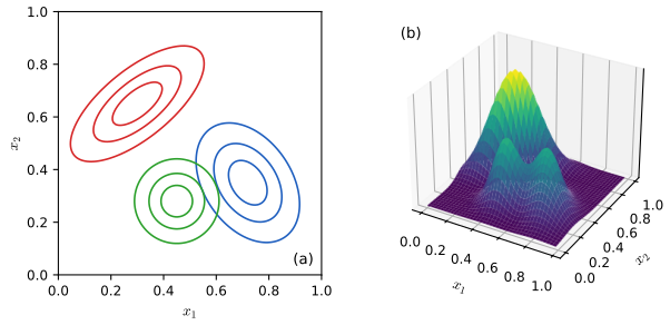
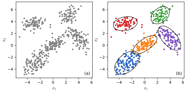
See also. Volume 1, Section 21.4 (mixtures by EM, choosing \(K\)), All of Statistics for the EM algorithm.
28.2.2 Bernoulli mixture models
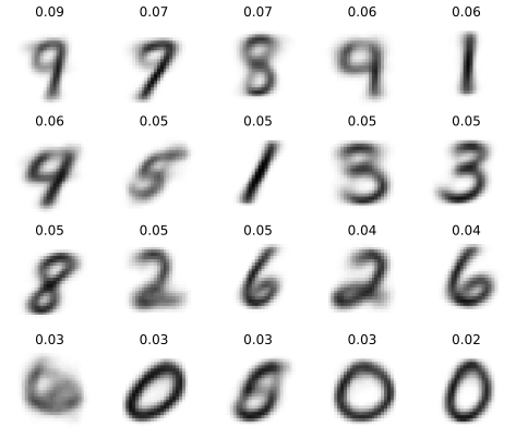
p. 932 For binary vectors, \(p(\bm x\given z=k)=\prod_d\mu_{dk}^{x_d}(1-\mu_{dk})^{1-x_d}\) (28.11), where \(\mu_{dk}\) is the probability that bit \(d\) is on in cluster \(k\). The EM updates are in Volume 1, gap 21.15: \(r_{nk}\propto\pi_k\prod_d\mu_{dk}^{x_{nd}}(1-\mu_{dk})^{1-x_{nd}}\), \(\pi_k=\frac1N\sum_nr_{nk}\), \(\mu_{dk}=\sum_nr_{nk}x_{nd}/\sum_nr_{nk}\). Figure 28.3 fits 20 components to binarised MNIST digits without using the labels; some digits are represented several times because the model does not know the true number of classes, and one component can end up (almost) empty.
28.2.3 Gaussian scale mixtures (GSMs)
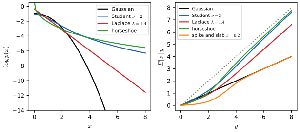
pp. 932–934 A Gaussian scale mixture is an "infinite" mixture of Gaussians with different scales: \(x=\epsilon z\) with \(z\sim\N(0,\sigma_0^2)\) and \(\epsilon\sim p(\epsilon)\), so that \(x\given\epsilon\sim\N(0,\epsilon^2\sigma_0^2)\) and \(p(x)=\int\N(x\given 0,\sigma_0^2\epsilon^2)p(\epsilon)\,\d\epsilon\) (28.12). The expanded parameterisation is computationally convenient (given \(\epsilon\) everything is Gaussian), and the choice of \(p(\epsilon)\) produces the sparsity-promoting priors used throughout the book:
- Student (28.13): \(\epsilon^2\sim\mathrm{IG}(\nu/2,\nu/2)\) gives \(\mathcal T(x\given 0,\sigma^2,\nu)\), heavier tails than a Gaussian of the same variance, and a Gaussian when \(\nu\to\infty\) (the inverse gamma collapses to a point mass). Proved, with the moments and tails, in gap 2.3.
- Laplace (28.14): \(\epsilon^2\sim\mathrm{Exp}(\lambda^2/2)\) (a gamma with shape 1) gives the density \(\frac\lambda2e^{-\lambda|x|}\) (here "Laplace\((x\given0,\lambda)\)" means rate \(\lambda\), i.e. scale \(1/\lambda\), the convention of (28.158)); proved in gap 15.9.
- Spike and slab (28.15): \(\epsilon\sim\mathrm{Ber}(\pi)\) gives \(\pi\N(x\given0,\sigma_0^2)+(1-\pi)\delta_0(x)\) (gap 15.8).
- Horseshoe: \(\epsilon\sim\mathrm{C}^+(1)\), a pole at 0 like the Student and Laplace but with polynomial tails that do not die away (gap 15.10).
What none of these references states is the rule the prior induces when it is used to clean up a noisy observation, which is the reason sparsity priors are used. That is the next gap box and the first demonstration.
Filling the gap 28.1: every scale mixture shrinks, and how much it shrinks (own result) pp. 932–934, Section 28.2.3
Proof
Let \(x\) have a scale-mixture prior and observe \(y=x+n\) with \(n\sim\N(0,s^2)\) independent. Write \(p_Y=p_X*\N(0,s^2)\) for the marginal of \(y\).
(i) The shrinkage factor. Given the scale \(\epsilon\), \(x\given\epsilon\sim\N(0,\epsilon^2\sigma_0^2)\), so by the Gaussian product rule \(\E[x\given y,\epsilon]=y\,\kappa(\epsilon)\) with \(\kappa(\epsilon)=\epsilon^2\sigma_0^2/(\epsilon^2\sigma_0^2+s^2)\in(0,1)\). The posterior of the scale is \(p(\epsilon\given y)\propto p(\epsilon)\,\N(y\given0,\epsilon^2\sigma_0^2+s^2)\). Hence \[ \E[x\given y]=y\;\E[\kappa(\epsilon)\given y],\qquad 0<\E[\kappa(\epsilon)\given y]<1, \] so the posterior mean has the sign of \(y\) and is smaller in magnitude: scale mixtures can only shrink. A large \(|y|\) is more probable under a large scale, which raises \(\E[\kappa\given y]\): the shrinkage factor increases with \(|y|\) and the heavier the tail of \(p(\epsilon)\), the faster.
(ii) Tweedie's formula. For any prior \(p_X\), differentiate under the integral: \(\partial_yp_Y(y)=\int p_X(x)\,\partial_y\N(y-x\given0,s^2)\,\d x=-\frac1{s^2}\int(y-x)p_X(x)\N(y-x\given0,s^2)\,\d x=-\frac{1}{s^2}\,p_Y(y)\,\big(y-\E[x\given y]\big)\), because \(p_X(x)\N(y-x)/p_Y(y)\) is the posterior density of \(x\). Therefore \[ \E[x\given y]=y+s^2\,\frac{\d}{\d y}\log p_Y(y). \] The shrinkage rule is fixed by the log-density of the noisy variable.
(iii) Tails. For the Laplace prior \(p_X=\frac\lambda2e^{-\lambda|x|}\), completing the square gives \(p_Y(y)=\frac\lambda2e^{\lambda^2s^2/2}\big[e^{-\lambda y}\Phi\big(\tfrac{y-\lambda s^2}{s}\big)+e^{\lambda y}\Phi\big(\tfrac{-y-\lambda s^2}s\big)\big]\), so for \(y\gg\lambda s^2\) the first term dominates, \((\log p_Y)'\to-\lambda\) and \(\E[x\given y]\to y-\lambda s^2\): a constant bias, exactly the lasso soft threshold shift. For a Student prior with \(\nu\) degrees of freedom \(p_Y(y)\propto|y|^{-(\nu+1)}\) for large \(|y|\) (a convolution with a Gaussian leaves a polynomial tail unchanged to leading order), so \(\E[x\given y]\approx y-(\nu+1)s^2/y\); the horseshoe has density \(\sim c/x^2\) in the tails, which gives \(\E[x\given y]\approx y-2s^2/y\). Heavy tails therefore leave large observations almost untouched, while the pole at 0 pulls small observations strongly towards 0: the point of the horseshoe, "kills small parameters but does not over-regularise large ones".
(iv) Spike and slab, closed form. With the spike \(\delta_0\) at probability \(1-\pi\) and slab \(\N(0,\sigma_0^2)\), \(y\) has density \(\pi\N(y\given0,\sigma_0^2+s^2)+(1-\pi)\N(y\given0,s^2)\), the posterior probability of the slab is \(w(y)=\pi\N(y\given0,\sigma_0^2+s^2)/p_Y(y)\), and \(\E[x\given y]=w(y)\,y\,\sigma_0^2/(\sigma_0^2+s^2)\). The posterior probability that \(x=0\) exactly is \(1-w(y)\). Note that the posterior mean is never exactly 0 for any of these priors when \(y\ne0\); exact zeros appear only in the posterior mode (the lasso) or in the posterior probability of the spike.
With \(s=1\), \(\sigma_0=1\) and \(y=3\), the four rules give 1.670 (Laplace, \(\lambda=1.4\)), 2.113 (Student, \(\nu=2\)), 2.210 (horseshoe) and 0.940 (spike and slab, \(\pi=0.2\)), against 1.5 for a Gaussian prior; at \(y=12\) the Laplace rule returns 10.60, as (iii) predicts (confirmed numerically by quadrature; Figure 28.x1).
28.2.4 Using GMMs as a prior for inverse imaging problems
pp. 934–937 Suppose we want a clean image \(\bm x\) from a corrupted \(\bm y\) with the linear-Gaussian forward model \(p(\bm y\given\bm x)=\N(\bm y\given\bm W\bm x,\sigma^2\bm I)\) (28.16), where \(\bm W=\bm I\) (additive noise, denoising), a convolution (deblurring), a diagonal 0/1 matrix (occlusion, inpainting) or a downsampling operator (super-resolution). The problem is ill-posed, so a prior is needed. Zoran and Weiss (2011) split the image into patches \(\bm x_i=\bm P_i\bm x\) and give each a GMM prior \(p(\bm x_i)=\sum_kp(c_i=k)\N(\bm x_i\given\bm\mu_k,\bm\Sigma_k)\) (200 components, trained on 2 million clean patches). The marginal likelihood of a corrupted patch under component \(c\) is \(\N(\bm y_i\given\bm W\bm\mu_c,\sigma^2\bm I+\bm W\bm\Sigma_c\bm W^{\mathrm T})\), so the MAP component is \[ c_i^*=\arg\max_cp(c)\,\N(\bm y_i\given\bm W\bm\mu_c,\sigma^2\bm I+\bm W\bm\Sigma_c\bm W^{\mathrm T}), \tag{28.17} \] and the patch is estimated with that component, \(p(\bm x_i\given\bm y_i)\approx p(\bm x_i\given\bm y_i,c_i^*)\propto\N(\bm x_i\given\bm\mu_{c^*_i},\bm\Sigma_{c^*_i})\N(\bm y_i\given\bm W\bm x_i,\sigma^2\bm I)\) (28.18). For whole images they minimise \[ E(\bm x\given\bm y)=\frac1{2\sigma^2}\|\bm W\bm x-\bm y\|^2-\mathrm{EPLL}(\bm x),\qquad\mathrm{EPLL}(\bm x)=\sum_i\log p(\bm P_i\bm x), \tag{28.19--28.20} \] the "expected patch log likelihood", by half-quadratic splitting. Because the patches overlap this is not a valid likelihood (it counts each pixel several times) but it works well. The method is explained next, and Figure 28.4 reproduces it on a smaller scale.
Filling the gap 28.2: the component marginal, the patch posterior and half-quadratic splitting pp. 934–935, (28.17)–(28.20)
Proof
The marginal (28.17). Given component \(c\), \(\bm y=\bm W\bm x+\bm n\) with \(\bm x\sim\N(\bm\mu_c,\bm\Sigma_c)\) and independent \(\bm n\sim\N(\bm0,\sigma^2\bm I)\) is a linear function of Gaussians, hence Gaussian with mean \(\bm W\bm\mu_c\) and covariance \(\bm W\bm\Sigma_c\bm W^{\mathrm T}+\sigma^2\bm I\) (the Gaussian marginal rule, gap 2.10). Bayes' rule gives the exact component posterior \(p(c\given\bm y)\propto p(c)\N(\bm y\given\bm W\bm\mu_c,\sigma^2\bm I+\bm W\bm\Sigma_c\bm W^{\mathrm T})\). The exact posterior of the patch is the mixture \(p(\bm x\given\bm y)=\sum_cp(c\given\bm y)p(\bm x\given\bm y,c)\), and the minimum mean-squared-error estimate is \(\sum_cp(c\given\bm y)\hat{\bm x}_c\); (28.17)–(28.18) replace it by the component with the largest weight, the hard version.
The patch posterior (28.18). Multiplying the two Gaussians in \(\bm x\): the posterior is \(\N(\bm m_c,\bm V_c)\) with \(\bm V_c^{-1}=\bm\Sigma_c^{-1}+\sigma^{-2}\bm W^{\mathrm T}\bm W\) and \(\bm m_c=\bm V_c(\bm\Sigma_c^{-1}\bm\mu_c+\sigma^{-2}\bm W^{\mathrm T}\bm y)\). For denoising (\(\bm W=\bm I\)) and a zero-mean component this equals the Wiener filter \[ \hat{\bm x}=\bm\Sigma_c(\bm\Sigma_c+\sigma^2\bm I)^{-1}\bm y, \] which in the eigenbasis \(\bm\Sigma_c=\bm V\bm\Lambda\bm V^{\mathrm T}\) multiplies the coordinate along \(\bm v_d\) by \(\lambda_d/(\lambda_d+\sigma^2)\): directions in which the component has variance far above the noise are kept, directions far below it are removed.
Half-quadratic splitting. The energy (28.19) is awkward because \(\log p(\bm P_i\bm x)\) is the log of a sum. Introduce an auxiliary patch \(\bm z_i\) for each patch and penalise \(\bm P_i\bm x\ne\bm z_i\): \[ E_\beta(\bm x,\{\bm z_i\})=\frac\lambda2\|\bm W\bm x-\bm y\|^2+\frac\beta2\sum_i\|\bm P_i\bm x-\bm z_i\|^2-\sum_i\log p(\bm z_i),\qquad\lambda=\frac1{\sigma^2}, \] which tends to \(E\) when \(\beta\to\infty\). Minimising alternately: (a) for fixed \(\bm x\), each patch separately minimises \(\frac\beta2\|\bm u_i-\bm z\|^2-\log p(\bm z)\) with \(\bm u_i=\bm P_i\bm x\); this is the MAP problem for a patch \(\bm z\) observed as \(\bm u_i=\bm z+\) noise of variance \(1/\beta\), so with the component chosen as in (28.17) (identity \(\bm W\), noise variance \(1/\beta\): \(c^*=\arg\max_c\pi_c\N(\bm u_i\given\bm0,\bm\Sigma_c+\bm I/\beta)\)) the minimiser is the Wiener estimate \(\bm z_i=\bm\Sigma_c(\bm\Sigma_c+\bm I/\beta)^{-1}\bm u_i\). (b) For fixed patches, the energy is quadratic in \(\bm x\), and setting the gradient to zero gives \((\lambda\bm W^{\mathrm T}\bm W+\beta\sum_i\bm P_i^{\mathrm T}\bm P_i)\bm x=\lambda\bm W^{\mathrm T}\bm y+\beta\sum_i\bm P_i^{\mathrm T}\bm z_i\). Since \(\sum_i\bm P_i^{\mathrm T}\bm P_i\) is diagonal (it counts how many patches contain each pixel) and \(\bm W\) is the identity or a 0/1 diagonal matrix for denoising and inpainting, the update is a pixelwise division. The schedule \(\beta\in\frac1{\sigma^2}\{1,4,8,16,32,64,128\}\) is increased gradually. My code subtracts each patch's mean before applying the zero-mean components, as the original method does, and adds it back.
On sample photographs (a 20-component, zero-mean prior fitted by my EM code to 40 000 \(8\times8\) patches of one photograph, tested on a crop of the other), noise of standard deviation 0.1 and the above schedule raise the PSNR from 20.0 dB to 25.9 dB; with half of the pixels removed (\(\bm W\) a 0/1 diagonal, \(\sigma=0.01\), \(\beta\) from 20 to 2560) the PSNR rises from 16.4 dB (missing pixels set to the mean) to 23.7 dB. The Wiener formula and the Gaussian marginal were confirmed numerically.
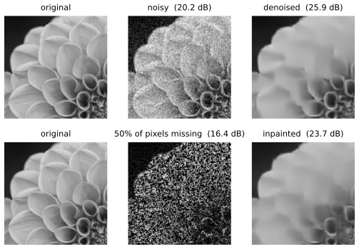
pp. 935–937 Two further remarks of the book. A principled treatment of overlapping patches uses a multiscale model or Gibbs sampling over patches, which also produces posterior samples (so a grey-scale input gets a colour output, which the posterior mode cannot). Section 28.2.4.2 trains an amortised inference network on the pairs \((\bm y,f(\bm y))\) from this procedure, or a discriminative network directly on \((\bm y,\bm x)\) pairs; the latter is limited by the corruptions it was trained on. Section 28.2.4.3 treats blind inverse problems (\(\bm W\) unknown) by EM-like alternation of \(\hat{\bm x}=\arg\max p(\bm x\given\bm y,\hat{\bm W})\) and \(\hat{\bm W}=\arg\max p(\bm y\given\hat{\bm x},\bm W)\), and cycle consistency when two noisy copies of the same image are available.
28.2.4.1 Why does the method work?
p. 936, (28.21)–(28.22) For a zero-mean component, the log prior of a patch is \(\log\N(\bm x\given\bm0,\bm\Sigma_k)=-\frac12\bm x^{\mathrm T}\bm\Sigma_k^{-1}\bm x+a_k\) (the book omits the factor \(\frac12\)), and with \(\bm\Sigma_k=\bm V_k\bm\Lambda_k\bm V_k^{\mathrm T}\) \[ \log p(\bm x\given c=k)=-\frac12\sum_{d=1}^D\frac1{\lambda_{k,d}}\big(\bm v_{k,d}^{\mathrm T}\bm x\big)^2+a_k. \tag{28.22} \] The eigenvectors act as templates: the cost of a patch is the sum of its squared projections on the templates, each weighted by the inverse eigenvalue, so a template with a small eigenvalue is expensive to use (a patch containing much of it is implausible under this component), while one with a large eigenvalue is cheap.
Filling the gap 28.3: what the fitted components look like, and why denoising over-smooths flat areas pp. 936–937, Figure 28.5
Proof
(28.22) is the Gaussian log-density rewritten in the eigenbasis: \(\bm x^{\mathrm T}\bm\Sigma^{-1}\bm x=\bm x^{\mathrm T}\bm V\bm\Lambda^{-1}\bm V^{\mathrm T}\bm x=\sum_d(\bm v_d^{\mathrm T}\bm x)^2/\lambda_d\). Combined with the Wiener gain \(\lambda_d/(\lambda_d+\sigma^2)\) of gap 28.2, a component acts as a bank of templates, each kept in proportion to how far its eigenvalue exceeds the noise.
Figure 28.5 shows what the fitted components contain. In my prior the largest component (weight 0.39) is the flat component: its largest eigenvalue is \(8\times10^{-4}\), far below \(\sigma^2=0.01\), so at \(\sigma=0.1\) its Wiener gain is at most \(0.07\) in every direction and any patch assigned to it is replaced by its mean. Other components keep 19 to 54 of the 64 templates above the noise level (edges at different orientations, textures). The patch step assigns a patch to a component by the marginal likelihood \(\N(\bm u\given\bm0,\bm\Sigma_c+\bm I/\beta)\), which prefers the flat component whenever \(\|\bm u\|^2\) is small compared with \(1/\beta\) per pixel; this is what produces the over-smooth flat areas in Figure 28.4 when the prior has seen only one photograph (the original method has 200 components and 2 million patches).
Footnote 7 and Section 28.6.5 say that PCA on natural patches gives sinusoids; the reason is proved in gap 28.19.

28.2.5 Using mixture models for classification problems
pp. 937–939 A mixture can be the class-conditional density of a generative classifier: \(p(y=c\given\bm x)=p(y=c)p(\bm x\given y=c)/Z\) (28.23), with \(p(\bm x\given y=c)=\sum_{k=1}^{K_c}\alpha_{c,k}\N(\bm x\given\bm\mu_{c,k},\bm\Sigma_{c,k})\) (28.24) for real features. Generative classifiers handle missing features (marginalise \(\bm x_m\): \(p(\bm x_v\given y=c)\)) and semi-supervised data (fit \(\sum\log p(\bm x^l,y^l)\) on labelled and \(\sum\log p(\bm x^u)\) on unlabelled data), but classify worse than discriminative models, which spend no capacity on irrelevant details of \(\bm x\) (Volume 1, Chapter 9). The hybrid objective of Bouchard and Triggs (2004), \[ \mathcal L(\bm\theta)=-\lambda\sum_n\log p(\bm x_n,y_n\given\bm\theta)-(1-\lambda)\sum_n\log p(y_n\given\bm x_n,\bm\theta),\quad0\le\lambda\le1, \tag{28.25} \] interpolates (with \(\kappa\) weighting labelled against unlabelled data in the generative term, (28.26)). To optimise it unconstrainedly the book uses softmax logits for \(\bm\pi\) and \(\alpha_{c,k}\), softplus for diagonal variances, and the diagonal-plus-low-rank covariance \(\bm\Sigma_{c,k}=\mathrm{diag}(\bm d_{c,k})+\bm S_{c,k}\bm S_{c,k}^{\mathrm T}\) (28.27) with \(\bm S\in\R^{D\times R}\), \(R\ll D\) (plus \(\epsilon\bm I\) for stability), and evaluates every log density with the log-sum-exp trick (28.28)–(28.30) and the two lemmas (28.31)–(28.32).
Filling the gap 28.4: log-sum-exp, the determinant and inversion lemmas, and what (28.25) really weights pp. 938–939, (28.25), (28.28)–(28.32)
Proof
Log-sum-exp (28.29). For any real \(M\), \(\log\sum_ke^{\beta_k}=\log\big(e^M\sum_ke^{\beta_k-M}\big)=M+\log\sum_ke^{\beta_k-M}\). With \(M=\max_k\beta_k\) every exponent \(\beta_k-M\le0\) and at least one equals 0, so the sum lies in \([1,K]\) and neither underflows to 0 nor overflows; the naive sum underflows when all \(\beta_k\lesssim-745\) in double precision (for example \(\beta_k\approx-10^5\), where the stable formula returns \(-10^5+\log(1+e^{-3}+e^{-10})\)). The class posterior (28.30) is the same trick applied over classes, and \(\log p(\bm x)=\log\tilde Z+L\).
Determinant lemma (28.31). For invertible \(\bm A\) (\(D\times D\)) and \(\bm S\in\R^{D\times R}\), consider \(\bm M=\begin{pmatrix}\bm A&-\bm S\\\bm S^{\mathrm T}&\bm I\end{pmatrix}\). Eliminating the lower-left block gives \(\det\bm M=\det\bm A\,\det(\bm I+\bm S^{\mathrm T}\bm A^{-1}\bm S)\) (Schur complement of \(\bm A\)); eliminating the upper-right block gives \(\det\bm M=\det\bm I\,\det(\bm A+\bm S\bm S^{\mathrm T})\) (Schur complement of \(\bm I\)). Equating the two proves \(\det(\bm A+\bm S\bm S^{\mathrm T})=\det(\bm I+\bm S^{\mathrm T}\bm A^{-1}\bm S)\det\bm A\).
Inversion lemma (28.32). Let \(\bm B=\bm A^{-1}-\bm A^{-1}\bm S\bm G^{-1}\bm S^{\mathrm T}\bm A^{-1}\) with \(\bm G=\bm I+\bm S^{\mathrm T}\bm A^{-1}\bm S\). Then \((\bm A+\bm S\bm S^{\mathrm T})\bm B=\bm I-\bm S\bm G^{-1}\bm S^{\mathrm T}\bm A^{-1}+\bm S\bm S^{\mathrm T}\bm A^{-1}-\bm S\bm S^{\mathrm T}\bm A^{-1}\bm S\bm G^{-1}\bm S^{\mathrm T}\bm A^{-1}\), and using \(\bm S^{\mathrm T}\bm A^{-1}\bm S=\bm G-\bm I\) in the last term, \(\bm S\bm S^{\mathrm T}\bm A^{-1}\bm S\bm G^{-1}=\bm S(\bm G-\bm I)\bm G^{-1}=\bm S-\bm S\bm G^{-1}\), so the sum collapses to \(\bm I\). For diagonal \(\bm A\) (as here and in factor analysis) the cost drops from \(O(D^3)\) to \(O(R^3+R^2D)\); see also gap 18.15, where the same lemmas are used for sparse GPs. Both lemmas and log-sum-exp were confirmed numerically (\(D=30\), \(R=4\)).
What the hybrid objective weights. Since \(\log p(\bm x,y)=\log p(y\given\bm x)+\log p(\bm x)\), (28.25) with all data labelled equals \(-\sum_n\log p(y_n\given\bm x_n)-\lambda\sum_n\log p(\bm x_n)\): the discriminative likelihood plus a regulariser \(-\lambda\sum_n\log p(\bm x_n)\), the marginal likelihood of the inputs. \(\lambda=0\) is a discriminative classifier, \(\lambda=1\) the generative one, and \(\lambda\) is the weight the model is made to give to explaining \(\bm x\) as well as \(y\).
28.2.6 Unidentifiability
p. 939 The parameters of a mixture are not identifiable because of label switching: relabelling the components leaves \(p(\bm x\given\bm\theta)\) unchanged, so the likelihood has (at least) \(K!\) equal modes, and the posterior mean of a component parameter such as \(\bm\mu_k\) averages over them and is meaningless. Stephens (2000) proposes a decision-theoretic fix: choose the action (a clustering or a parameter set) after a suitable permutation of the labels. The symmetry and the legitimacy of an ordering constraint are proved in Volume 1, gap 21.13; permuting the components of a fitted GMM was confirmed to leave the log-likelihood unchanged to \(10^{-8}\). The same symmetry makes the topic-label ambiguity of Figure S28.2 below.
28.3 Factor analysis
p. 940 Factor analysis (FA) has a Gaussian prior and a Gaussian likelihood with a linear mean. Most of this section is proved in Volume 1, so the notes below state the model, give the book's equation numbers, point to the proofs and spend their effort on what the book adds.
28.3.1 Factor analysis: the basics
pp. 940–944 The model is \(p(\bm z)=\N(\bm\mu_0,\bm\Sigma_0)\), \(p(\bm x\given\bm z)=\N(\bm W\bm z+\bm\mu,\bm\Psi)\) (28.33)–(28.34), with a \(D\times L\) factor loading matrix \(\bm W\) and diagonal \(\bm\Psi\). The marginal is \(\N(\bm W\bm\mu_0+\bm\mu,\bm\Psi+\bm W\bm\Sigma_0\bm W^{\mathrm T})\) (28.36), so one may take \(\bm\mu_0=\bm0\) and \(\bm\Sigma_0=\bm I\) (absorb \(\bm\Sigma_0^{1/2}\) into \(\bm W\), (28.38)), giving \[ p(\bm z)=\N(\bm 0,\bm I),\quad p(\bm x\given\bm z)=\N(\bm W\bm z+\bm\mu,\bm\Psi),\quad p(\bm x)=\N(\bm\mu,\bm W\bm W^{\mathrm T}+\bm\Psi). \tag{28.39--28.41} \] Thus FA is a low-rank-plus-diagonal Gaussian with \(O(LD)\) parameters between a diagonal (\(O(D)\)) and a full covariance (\(O(D^2)\)); \(\bm\Psi\) must be diagonal, otherwise \(\bm W=\bm0\) would already fit any covariance. The reduction to this normal form and the two forms of the posterior \(\N(\bm\mu_{z|x},\bm\Sigma_{z|x})\), \(\bm\Sigma_{z|x}=(\bm I+\bm W^{\mathrm T}\bm\Psi^{-1}\bm W)^{-1}=\bm I-\bm W^{\mathrm T}(\bm W\bm W^{\mathrm T}+\bm\Psi)^{-1}\bm W\), \(\bm\mu_{z|x}=\bm\Sigma_{z|x}\bm W^{\mathrm T}\bm\Psi^{-1}(\bm x-\bm\mu)\) (28.43)–(28.45), are proved in Volume 1, gap 20.6.
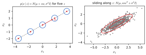
Fast likelihood (28.46)–(28.50). With \(\bm C=\bm W\bm W^{\mathrm T}+\bm\Psi\) and \(\bm L=\bm I+\bm W^{\mathrm T}\bm\Psi^{-1}\bm W\) (an \(L\times L\) matrix), the inversion lemma gives \(\bm C^{-1}=\bm\Psi^{-1}-\bm\Psi^{-1}\bm W\bm L^{-1}\bm W^{\mathrm T}\bm\Psi^{-1}\) and the determinant lemma \(\log\det\bm C=\log\det\bm L+\log\det\bm\Psi\) (both proved in gap 28.4), so \(\log p(\bm x\given\bm\mu,\bm C)=-\frac12[D\log2\pi+\log\det\bm C+\tilde{\bm x}^{\mathrm T}\bm C^{-1}\tilde{\bm x}]\) (28.48) costs \(O(L^3+LD)\) per observation, not \(O(D^3)\). My fa_loglik uses exactly this and agrees with the full-covariance Gaussian density to \(10^{-8}\).
EM (28.51)–(28.58). The E step computes \(\E[\bm z\given\bm x]=\bm B\bm x\) and \(\E[\bm z\bm z^{\mathrm T}\given\bm x]=\bm I-\bm B\bm W+\bm B\bm x\bm x^{\mathrm T}\bm B^{\mathrm T}\) with \(\bm B=\bm W^{\mathrm T}\bm C^{-1}\) (28.54)–(28.56); the M step is \(\bm W^{\rm new}=\bm E_{x,z}\bm E_{z,z}^{-1}\), \(\bm\Psi^{\rm new}=\frac1N\mathrm{diag}(\bm E_{x,x}-\bm W^{\rm new}\bm E_{x,z}^{\mathrm T})\) (28.57)–(28.58), derived in Volume 1, gap 20.8. The M step is the regression of \(\bm x\) on the expected latent variables (the maximum likelihood fit of a multi-output linear regression with the unknown inputs replaced by expected sufficient statistics), and the positivity of \(\bm\Psi\) is automatic. My EM (the \(K=1\) case of MFA) increases the log-likelihood at every iteration and reaches the same value as the library routine (\(-10.1355\) per observation on a simulated set).
28.3.1.5 Handling missing data
p. 943, (28.59)–(28.61) Under missingness at random (Section 3.11 of the book) the posterior of \(\bm z\) given the observed coordinates \(\bm x_1\) uses only the rows \(\bm W_1\) of \(\bm W\) that belong to them: \(\bm\Sigma_{z|1}^{-1}=\bm I+\bm W_1^{\mathrm T}\bm\Sigma_{11}^{-1}\bm W_1\) and \(\bm\mu_{z|1}=\bm\Sigma_{z|1}\bm W_1^{\mathrm T}\bm\Sigma_{11}^{-1}(\bm x_1-\bm\mu_1)\), where \(\bm\Sigma_{11}\) is the corresponding block of the diagonal \(\bm\Psi\). The book says EM is modified "in the obvious way". Here it is.
Filling the gap 28.5: EM for factor analysis when coordinates are missing p. 943, (28.59)–(28.61)
Proof
Let \(O_n\) be the set of observed coordinates of case \(n\) and write \(\tilde{\bm z}=(\bm z;1)\), \(\tilde{\bm w}_d=(\bm w_d;\mu_d)\), so that \(x_{nd}\given\bm z_n\sim\N(\tilde{\bm w}_d^{\mathrm T}\tilde{\bm z}_n,\psi_d)\), independently over \(d\) (\(\bm\Psi\) is diagonal).
Observed-data likelihood. Because the coordinates are conditionally independent given \(\bm z\), integrating \(\bm z\) out of the observed ones gives \(\N(\bm x_{O},\bm\mu_O,\bm W_O\bm W_O^{\mathrm T}+\bm\Psi_O)\) (a sub-block of the Gaussian (28.41)), and the missing coordinates marginalise to 1 (MAR: the missingness mechanism factors out).
E step. The posterior of \(\bm z_n\) given \(\bm x_{O_n}\) is Gaussian with covariance \(\bm\Sigma_n=(\bm I+\bm W_{O_n}^{\mathrm T}\bm\Psi_{O_n}^{-1}\bm W_{O_n})^{-1}\) and mean \(\bm m_n=\bm\Sigma_n\bm W_{O_n}^{\mathrm T}\bm\Psi_{O_n}^{-1}(\bm x_{O_n}-\bm\mu_{O_n})\), giving \(\E[\tilde{\bm z}_n]=(\bm m_n;1)\) and \(\E[\tilde{\bm z}_n\tilde{\bm z}_n^{\mathrm T}]=\begin{pmatrix}\bm\Sigma_n+\bm m_n\bm m_n^{\mathrm T}&\bm m_n\\\bm m_n^{\mathrm T}&1\end{pmatrix}\).
M step. Take as complete data \((\bm x_{O_n},\bm z_n)\) and integrate the missing coordinates out analytically: given \(\bm z_n\) they are independent of the observed ones, so they marginalise to 1 and contribute nothing to the complete-data likelihood \(\prod_n\big[p(\bm z_n)\prod_{d\in O_n}\N(x_{nd}\given\tilde{\bm w}_d^{\mathrm T}\tilde{\bm z}_n,\psi_d)\big]\). (Treating them as additional latent variables is also a valid EM but converges more slowly.) The expected complete-data log-likelihood is \(\sum_n\sum_{d\in O_n}[-\frac12\log\psi_d-\frac1{2\psi_d}\E(x_{nd}-\tilde{\bm w}_d^{\mathrm T}\tilde{\bm z}_n)^2]\), which separates over \(d\) and involves only the cases in which coordinate \(d\) was observed, \(\mathcal N_d=\{n:d\in O_n\}\). Maximising each term (a weighted least-squares problem in \(\tilde{\bm w}_d\)): \[ \tilde{\bm w}_d^{\rm new}=\Big(\sum_{n\in\mathcal N_d}x_{nd}\,\E[\tilde{\bm z}_n]^{\mathrm T}\Big)\Big(\sum_{n\in\mathcal N_d}\E[\tilde{\bm z}_n\tilde{\bm z}_n^{\mathrm T}]\Big)^{-1},\quad\psi_d^{\rm new}=\frac1{|\mathcal N_d|}\sum_{n\in\mathcal N_d}\Big[x_{nd}^2-2x_{nd}\tilde{\bm w}_d^{{\rm new}\mathrm T}\E\tilde{\bm z}_n+\tilde{\bm w}_d^{{\rm new}\mathrm T}\E[\tilde{\bm z}_n\tilde{\bm z}_n^{\mathrm T}]\tilde{\bm w}_d^{\rm new}\Big], \] which for complete data is (28.57)–(28.58) row by row (a separate regression for each output coordinate; the mean is updated jointly with the loadings by appending the 1 to \(\bm z\)). Monotonicity is the general EM argument (gap 6.14) with latent variable \(\bm z_n\) and observed \(\bm x_{O_n}\).
(The conditional-mean imputation of missing entries followed by a complete-data fit is not EM: it forgets the posterior variance \(\bm\Sigma_n\) of the latent code, which enters \(\E[\tilde{\bm z}\tilde{\bm z}^{\mathrm T}]\); see gap 6.15.)
28.3.1.6 Unidentifiability of the parameters
pp. 943–944, (28.62)–(28.64) If \(\tilde{\bm W}=\bm W\bm R\) with \(\bm R\bm R^{\mathrm T}=\bm I\) then \(\tilde{\bm W}\tilde{\bm W}^{\mathrm T}=\bm W\bm W^{\mathrm T}\), so the loadings and the latent factors are identifiable only up to a rotation (the "factor rotations problem"); the same \(\bm R\) rotates \(\bm z\), which has an isotropic prior. Ways to break the symmetry, in the book's order: orthogonal columns in decreasing order of eigenvalue (PPCA, still ambiguous in sign); a lower-triangular \(\bm W\) with positive diagonal (28.64), which has \(D+DL-L(L-1)/2\) free parameters, exactly the number of identifiable parameters; sparsity-promoting priors on \(\bm W\) (\(\ell_1\), ARD, spike and slab: sparse FA); heuristic rotations that increase interpretability, such as varimax (the rotation that maximises the sum over columns of the variance of the squared loadings, which pushes each loading towards 0 or large); and non-Gaussian priors on \(\bm z\), which make \(\bm W\) identifiable (Section 28.6.2). The count is proved in Volume 1, gap 20.10; I confirmed it numerically as the rank of the Jacobian of \((\bm W,\bm\Psi)\mapsto\bm W\bm W^{\mathrm T}+\bm\Psi\) (rank 25 for \(D=7\), \(L=3\), equal to \(7\cdot4-3\)), and that \(\bm W\bm R\) leaves the likelihood unchanged.
28.3.2 Probabilistic PCA
pp. 944–946 Probabilistic PCA (PPCA, Tipping and Bishop 1999; "sensible PCA", Roweis 1997) is FA with orthogonal columns and \(\bm\Psi=\sigma^2\bm I\), so \(p(\bm x)=\N(\bm\mu,\bm C)\), \(\bm C=\bm W\bm W^{\mathrm T}+\sigma^2\bm I\). Its advantage over FA is a closed-form maximum, and over PCA a proper likelihood. The log-likelihood is \(-\frac N2[D\log2\pi+\log|\bm C|+\mathrm{tr}(\bm C^{-1}\bm S)]\) (28.66) with \(\hat{\bm\mu}=\bar{\bm x}\) and \(\bm S\) the empirical covariance; its maximum satisfies \[ \hat{\bm W}=\bm U_L(\bm\Lambda_L-\sigma^2\bm I)^{1/2}\bm R,\qquad\hat\sigma^2=\frac1{D-L}\sum_{i=L+1}^D\lambda_i \tag{28.67, 28.69} \] (\(\bm U_L,\bm\Lambda_L\): the top \(L\) eigenvectors and eigenvalues of \(\bm S\); \(\bm R\) an arbitrary orthogonal matrix), so \(\bm C=\bm U_L(\bm\Lambda_L-\sigma^2\bm I)\bm U_L^{\mathrm T}+\sigma^2\bm I\) (28.68) and \(\hat\sigma^2\) is the average discarded variance. In the noise-free limit \(\sigma^2\to0\), \(\hat{\bm W}=\bm U_L\bm\Lambda_L^{1/2}\) and \(\hat{\bm C}=\bm S_L\) is the rank-\(L\) approximation: ordinary PCA (28.70)–(28.71). That these are the global maximum (not just stationary points) is proved in Volume 1, gap 20.7.
Posterior (28.72)–(28.75). From the FA formulas with \(\bm\Psi=\sigma^2\bm I\), \(\bm\Sigma^{-1}=\bm I+\sigma^{-2}\bm W^{\mathrm T}\bm W=\sigma^{-2}\bm M\) with \(\bm M=\sigma^2\bm I+\bm W^{\mathrm T}\bm W\), so \(p(\bm z\given\bm x)=\N(\bm M^{-1}\bm W^{\mathrm T}(\bm x-\bm\mu),\sigma^2\bm M^{-1})\) (28.74); as \(\sigma^2\to0\) with \(\bm W\) of full column rank, \(\E[\bm z\given\bm x]\to(\bm W^{\mathrm T}\bm W)^{-1}\bm W^{\mathrm T}(\bm x-\bar{\bm x})\), the orthogonal projection of PCA (28.75), with zero posterior covariance. EM (28.76)–(28.79). In this limit EM is \(\tilde{\bm Z}=(\bm W^{\mathrm T}\bm W)^{-1}\bm W^{\mathrm T}\tilde{\bm X}\) (project) then \(\bm W=\tilde{\bm X}\tilde{\bm Z}^{\mathrm T}(\tilde{\bm Z}\tilde{\bm Z}^{\mathrm T})^{-1}\) (regress), which is the multi-output regression MLE with the expected latent variables as inputs. The claim "the only stable fixed point is the global optimum" is proved in Volume 1, gap 20.9 by showing that the column space of \(\bm W\) follows subspace iteration on \(\bm S\), with rate \(\lambda_{L+1}/\lambda_L\); the result of EM spans the principal subspace but is not orthonormal and must be orthogonalised (or modified to return the principal basis, Ahn and Oh 2003).
28.3.3 Mixture of factor analyzers
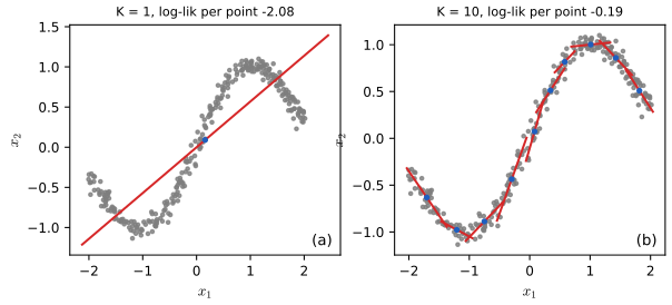
pp. 946–952 FA assumes a single linear map; a mixture of factor analysers (MFA, Ghahramani and Hinton 1996) lets the model be locally linear, a mixture of linear manifolds approximating a curved one, or equivalently a mixture of Gaussians in which every component has a diagonal-plus-low-rank covariance. Sample a component \(m_n\sim\mathrm{Cat}(\bm\pi)\), then \(\bm z_n\sim\N(\bm0,\bm I)\) and \(\bm x_n\given\bm z_n,m_n=k\sim\N(\bm\mu_k+\bm W_k\bm z_n,\bm\Psi)\) (28.80)–(28.82). Integrating out \(\bm z\),
\[ p(\bm x)=\sum_k\pi_k\N(\bm x\given\bm\mu_k,\bm\Psi+\bm W_k\bm W_k^{\mathrm T}), \tag{28.85} \]
and with \(\bm\Psi=\sigma^2\bm I\) a mixture of PPCA models (Figure 28.8). It needs \(O(KLD)\) parameters instead of \(O(KD^2)\). The E step is \(r_{ij}\propto\pi_j\N(\bm x_i\given\bm\mu_j,\bm W_j\bm W_j^{\mathrm T}+\bm\Psi)\) (28.86) with the component moments (28.87)–(28.88), and the M step updates the augmented loadings \([\bm W_j\ \bm\mu_j]\) by a responsibility-weighted regression (28.89)–(28.91), the shared noise by (28.92) and the weights by (28.93); the derivation (with the ECM variant) is in Volume 1, gap 20.11. My MFA class implements this, uses the lemma-based likelihood, and increases the log-likelihood at every iteration for both the diagonal and the isotropic \(\bm\Psi\) (with the isotropic update \(\sigma^2=\frac1D\mathrm{tr}\,\bm\Psi^{\rm new}\), the exact maximiser of the common-variance objective).
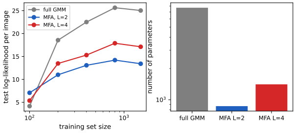
The parameter saving is a trade, not a free lunch. Figure 28.x3 compares a full-covariance GMM with MFAs on the 8×8 digits (\(K=5\)): the MFA uses \(5\times\)–\(9\times\) fewer parameters, and it generalises better only for very small training sets (\(N=100\)); with 800 or more training images the full-covariance mixture wins on held-out likelihood, so "less overfitting" is a statement about the small-sample regime.
28.3.3.3–28.3.3.4 Fitting by SGD, and model selection
p. 949 MFA can also be fitted by SGD on the log-likelihood (Richardson and Weiss 2018), which scales to huge \(D\) because of the lemma-based likelihood, or inside a deep autoencoder (Zong et al. 2018). To choose \(K\) and \(L\) one can search with the marginal or validation likelihood, or start from the maximal \(L\) and let automatic relevance determination (ARD) prune loading columns by variational Bayes EM (Bishop 1999; Ghahramani and Beal 2000; the ARD objective and its updates are in gap 15.11); Figures 28.9 and 28.10 (Beal 2003) show that the method recovers six clusters with intrinsic dimensions 7, 4, 3, 2, 2, 1 once there are at least 64 points per cluster, and fewer, simpler components with less data (the Bayesian Occam's razor). The number of components still needs a discrete search with birth and death moves (Ghahramani and Beal 2000), reversible-jump MCMC (Lopes and West 2004) or nonparametric priors with Gibbs sampling (Paisley and Carin 2009).
28.3.3.5 MixFA for image generation
pp. 949–953, (28.94)–(28.96) Richardson and Weiss (2018) fit an MFA to CelebA faces (\(K=300\), \(L=10\), \(D=64\times64\times3=12{,}288\)) by SGD, initialising \(\bm\mu_k\) by K-means and \(\bm W_k\) by factor analysis within each cluster, and find samples competitive with VAEs and GANs, better coverage of the modes of the data, an exact likelihood (so unusual images can be flagged, Figure 28.13) and imputation from any pattern of observed pixels (Figure 28.14): the most probable component is \(k^*=\arg\max_kp(c=k)p(\bm x_1\given c=k)\) with \(\log p(\bm x_1\given\bm\mu_k,\bm C_k)=-\frac12[D_1\log2\pi+\log\det\bm C_{k,11}+\tilde{\bm x}_1^{\mathrm T}\bm C_{k,11}^{-1}\tilde{\bm x}_1]\) (28.94)–(28.95), then \(\hat{\bm z}=\E[\bm z\given\bm x_1,k^*]\) by (28.59)–(28.61) and the completion \(\hat{\bm x}=\bm W_{k^*}\hat{\bm z}+\bm\mu_{k^*}\) (28.96), keeping the observed pixels. The next gap box derives these steps and the cost.
Filling the gap 28.6: the observed-data marginal, imputation by a mixture, the exact MMSE version, and the parameter counts pp. 946–953, (28.85), (28.94)–(28.96)
Proof
Marginal of a sub-vector. Within component \(k\), \(\bm x\sim\N(\bm\mu_k,\bm C_k)\), \(\bm C_k=\bm W_k\bm W_k^{\mathrm T}+\bm\Psi\), and the sub-vector of observed coordinates is \(\N(\bm\mu_{k,1},\bm C_{k,11})\) with \(\bm C_{k,11}=\bm W_{k,1}\bm W_{k,1}^{\mathrm T}+\bm\Psi_{11}\) (a Gaussian marginal, again low rank plus diagonal, so the lemmas of gap 28.4 apply with \(D_1\) in place of \(D\)). Hence \(p(\bm x_1)=\sum_k\pi_k\N(\bm x_1\given\bm\mu_{k,1},\bm C_{k,11})\) and \(p(k\given\bm x_1)\propto\pi_k\N(\bm x_1\given\bm\mu_{k,1},\bm C_{k,11})\), which gives \(k^*\) in (28.94).
The conditional mean within a component. Given \(k\) and \(\bm z\), the unobserved coordinates satisfy \(\bm x_2=\bm W_{k,2}\bm z+\bm\mu_{k,2}+\bm\epsilon_2\) with \(\bm\epsilon_2\) independent of \(\bm x_1\) (because \(\bm\Psi\) is diagonal), so \(\E[\bm x_2\given\bm x_1,k]=\bm W_{k,2}\E[\bm z\given\bm x_1,k]+\bm\mu_{k,2}\), which is (28.96) restricted to the missing block. This coincides with the Gaussian conditional mean \(\bm\mu_{k,2}+\bm C_{k,21}\bm C_{k,11}^{-1}(\bm x_1-\bm\mu_{k,1})\): for \(K=1\) I confirmed equality to \(10^{-8}\).
The exact estimate. The minimum mean-squared-error imputation is the average over components, \(\E[\bm x_2\given\bm x_1]=\sum_kp(k\given\bm x_1)\E[\bm x_2\given\bm x_1,k]\); the book's \(k^*\) rule is its hard version, which is accurate when one responsibility is close to 1 and discontinuous where two components tie.
Counts and costs. A full-covariance GMM has \(K\big(\tfrac{D(D+1)}2+D\big)+K-1\) parameters. An MFA with shared diagonal noise has \(K(DL+D)+D+K-1\) (means, loadings, shared \(\bm\Psi\), weights), reduced by \(KL(L-1)/2\) because each \(\bm W_k\) is identifiable only up to a rotation (gap 20.10 of Volume 1); with component-specific noise, \(K(DL+2D)+K-1\). With \(D=54\), \(K=5\): \(7699\) for the GMM against \(868\) (\(L=2\)) and \(1408\) (\(L=4\)) before the rotation correction. Per observation and component the likelihood costs \(O(L^3+LD)\) instead of \(O(D^3)\) after a one-off \(O(KD^3)\) for the GMM's Cholesky factors.
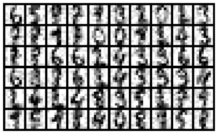
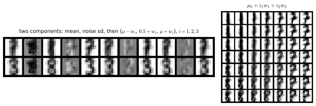
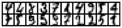
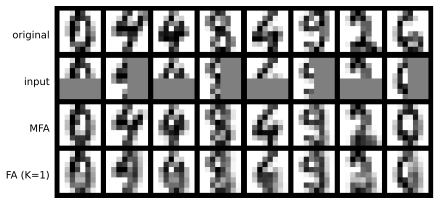
Stand-in for Figures 28.11 to 28.14: the same model with \(K=10\) components and \(L=4\) factors fitted to 1500 of the 1797 8×8 digit images (64 pixels, intensities in \([0,1]\), noise floor \(\psi_d\ge0.01\)). Its held-out log-likelihood is 35.5 per image (37.7 on training images), so it generalises well, and the four figures show the same four uses.
28.3.4 Factor analysis models for paired data
pp. 953–956 Now there are two views \(\bm x\in\R^{D_x}\) and \(\bm y\in\R^{D_y}\) (two sensors or modalities). Supervised PCA (Yu et al. 2006) shares one latent code, \(\bm z_n\sim\N(\bm0,\bm I_L)\), \(\bm x_n\given\bm z_n\sim\N(\bm W_x\bm z_n,\sigma_x^2\bm I)\), \(\bm y_n\given\bm z_n\sim\N(\bm W_y\bm z_n,\sigma_y^2\bm I)\) (28.97)–(28.99); with a prior on \((\bm W_x,\bm W_y,\sigma_x,\sigma_y)\) it is Bayesian factor regression (West 2003). For scalar \(y\), integrating out \(\bm z\) gives \(p(y\given\bm x)=\N(\bm x^{\mathrm T}\bm v,\bm w_y^{\mathrm T}\bm C\bm w_y+\sigma_y^2)\) (28.100) with \(\bm C=(\bm I+\sigma_x^{-2}\bm W_x^{\mathrm T}\bm W_x)^{-1}\), \(\bm v=\sigma_x^{-2}\bm W_x\bm C\bm w_y\) (28.101)–(28.102) (the book writes \(\bm C\bm W_x\bm w_y\), whose dimensions do not match). A logistic \(p(y\given\bm z)=\mathrm{Ber}(\sigma(\bm w_y^{\mathrm T}\bm z))\) (28.103) has no closed-form predictive, and the tilted likelihood \(p(\bm Y\given\bm Z)p(\bm X\given\bm Z)^\alpha p(\bm Z)\) (28.104), \(\alpha\le1\) (chosen by cross-validation), puts more weight on the target \(y\) when the aim is prediction through the bottleneck.
Partial least squares (PLS) is the asymmetric version: some variance of \(\bm x\) is explained by its own private subspace \(\bm z^x\), the rest by the shared \(\bm z^s\): \(p(\bm z)=\N(\bm z^s\given\bm0,\bm I)\N(\bm z^x\given\bm0,\bm I)\), \(\bm y\given\bm z\sim\N(\bm W_y\bm z^s+\bm\mu_y,\sigma^2\bm I)\), \(\bm x\given\bm z\sim\N(\bm W_x\bm z^s+\bm B_x\bm z^x+\bm\mu_x,\sigma^2\bm I)\) (28.105)–(28.107). Canonical correlation analysis (CCA) is the symmetric version with a private subspace for each view (28.111)–(28.113); the joint of \(\bm v=(\bm y;\bm x)\) (or \((\bm x;\bm y)\)) is \(\N(\bm\mu,\bm W\bm W^{\mathrm T}+\sigma^2\bm I)\) (28.108), (28.114) with the block structure (28.109)–(28.110), (28.115)–(28.116). Bach and Jordan (2005) showed that maximum likelihood in the CCA model is classical CCA (Hotelling 1936); generalisations are generalised CCA (several views), deep CCA and exponential-family CCA (Section 32.2.2.2).
Filling the gap 28.7: the predictive of supervised PCA, the joint covariance, and the likelihood of the CCA model as a reduced-rank regression pp. 953–956, (28.100)–(28.116)
Proof
(28.100)–(28.102). Given \(\bm x\), the posterior of \(\bm z\) is \(\N(\sigma_x^{-2}\bm C\bm W_x^{\mathrm T}\bm x,\bm C)\) with \(\bm C=(\bm I+\sigma_x^{-2}\bm W_x^{\mathrm T}\bm W_x)^{-1}\) (the FA posterior with \(\bm\Psi=\sigma_x^2\bm I\)). Since \(y=\bm w_y^{\mathrm T}\bm z+\epsilon_y\) with independent noise, \(p(y\given\bm x)\) is Gaussian with mean \(\sigma_x^{-2}\bm w_y^{\mathrm T}\bm C\bm W_x^{\mathrm T}\bm x=\bm x^{\mathrm T}\bm v\) and variance \(\bm w_y^{\mathrm T}\bm C\bm w_y+\sigma_y^2\), where \(\bm v=\sigma_x^{-2}\bm W_x\bm C\bm w_y\) (a \(D_x\)-vector); I confirmed it against the conditional of the joint Gaussian.
The joint (28.108)–(28.110). With \(\bm W=\begin{pmatrix}\bm W_y&\bm0\\\bm W_x&\bm B_x\end{pmatrix}\) acting on \((\bm z^s,\bm z^x)\) one gets \(\bm W\bm W^{\mathrm T}=\begin{pmatrix}\bm W_y\bm W_y^{\mathrm T}&\bm W_y\bm W_x^{\mathrm T}\\\bm W_x\bm W_y^{\mathrm T}&\bm W_x\bm W_x^{\mathrm T}+\bm B_x\bm B_x^{\mathrm T}\end{pmatrix}\); the cross-covariance has rank at most \(L_s\) and is carried entirely by the shared factor. The CCA case is analogous with a second private block.
Maximum likelihood is CCA (Bach and Jordan 2005), when the private covariances are unrestricted. Suppose \(L_x\ge D_x\), \(L_y\ge D_y\) (the "large enough" private subspaces) so that \(\bm\Sigma_{xx}\) and \(\bm\Sigma_{yy}\) are arbitrary positive definite matrices, with \(\bm\Sigma_{xy}\) of rank at most \(L_s\) (the isotropic \(\sigma^2\) in (28.112)–(28.113) is then absorbed by the private blocks). The model is exactly the set of Gaussians with these covariance blocks: given any positive definite \(\bm\Sigma\) with \(\mathrm{rank}\,\bm\Sigma_{xy}\le L_s\), write \(\bm R=\bm\Sigma_{xx}^{-1/2}\bm\Sigma_{xy}\bm\Sigma_{yy}^{-1/2}=\bm U_r\bm P\bm V_r^{\mathrm T}\) (thin SVD, \(\|\bm R\|<1\)) and set \(\bm W_x=\bm\Sigma_{xx}^{1/2}\bm U_r\bm P^{1/2}\), \(\bm W_y=\bm\Sigma_{yy}^{1/2}\bm V_r\bm P^{1/2}\); then \(\bm\Sigma_{xx}-\bm W_x\bm W_x^{\mathrm T}=\bm\Sigma_{xx}^{1/2}(\bm I-\bm U_r\bm P\bm U_r^{\mathrm T})\bm\Sigma_{xx}^{1/2}\succeq0\), so the remainder is a valid private covariance.
Factor the Gaussian as \(p(\bm x)p(\bm y\given\bm x)\): the parameters \(\bm\Sigma_{xx}\), the regression matrix \(\bm B=\bm\Sigma_{yx}\bm\Sigma_{xx}^{-1}\) (of rank \(\le L_s\)) and the conditional covariance \(\bm\Sigma_{y|x}\) vary independently. The likelihood therefore splits: \(\hat{\bm\Sigma}_{xx}=\bm S_{xx}\) (the usual Gaussian MLE), and \((\bm B,\bm\Sigma_{y|x})\) maximise a Gaussian reduced-rank regression likelihood. For fixed \(\bm B\) the MLE of \(\bm\Sigma_{y|x}\) is the residual covariance \(\bm E(\bm B)=\frac1N\sum_n(\bm y_n-\bm B\bm x_n)(\bm y_n-\bm B\bm x_n)^{\mathrm T}\), and the profile log-likelihood is \(-\frac N2\log\det\bm E(\bm B)+\mathrm{const}\), so we minimise \(\det\bm E(\bm B)\) over rank-\(r\) matrices \(\bm B\) (\(r=L_s\)). Whiten both views (\(\bm x'=\bm S_{xx}^{-1/2}\bm x\), \(\bm y'=\bm S_{yy}^{-1/2}\bm y\), which multiplies \(\det\bm E\) by the constant \(\det\bm S_{yy}^{-1}\)); then \(\frac1N\bm X'^{\mathrm T}\bm X'=\bm I\), the cross-covariance is \(\bm C=\bm S_{yy}^{-1/2}\bm S_{yx}\bm S_{xx}^{-1/2}\) with singular values \(\rho_1\ge\rho_2\ge\dots\) (the canonical correlations), and \[ \bm E=\bm I-\bm C\bm C^{\mathrm T}+(\bm B'-\bm C)(\bm B'-\bm C)^{\mathrm T}. \] Geometrically, the columns of \(\bm X'\bm B'^{\mathrm T}\) span at most an \(r\)-dimensional subspace \(\mathcal Q\) of the column space of \(\bm X'\), and the best fit to \(\bm Y'\) from \(\mathcal Q\) leaves residual \(\det\bm E\ge\prod_{i=1}^{r}(1-c_i^2)\), where \(c_1\ge c_2\ge\dots\ge c_r\) are the cosines of the principal angles between \(\mathrm{col}(\bm Y')\) and \(\mathcal Q\) (the residual of projecting the whitened \(\bm Y'\) on \(\mathcal Q\) has determinant \(\prod_i(1-c_i^2)\)). Write \(\mathcal Q\) with an orthonormal basis \(\bm Q=\bm X'\bm G/\sqrt N\) (\(\bm G\in\R^{D_x\times r}\), \(\bm G^{\mathrm T}\bm G=\bm I\), because \(\frac1N\bm X'^{\mathrm T}\bm X'=\bm I\)); the cosines are the singular values of \(\bm Y'^{\mathrm T}\bm Q/\sqrt N=\bm C\bm G\), and \(\sigma_i(\bm C\bm G)\le\sigma_i(\bm C)\|\bm G\|=\rho_i\). Hence \(\det\bm E\ge\prod_{i\le r}(1-\rho_i^2)\), with equality when \(\bm G\) holds the top \(r\) right singular vectors of \(\bm C\), i.e. when \(\mathcal Q\) is spanned by the top \(r\) canonical variates of \(\bm X\). With \(\bm C=\bm U\bm P\bm V^{\mathrm T}\) the minimiser is \(\bm B=\bm S_{yy}^{1/2}\bm U_r\bm P_r\bm V_r^{\mathrm T}\bm S_{xx}^{-1/2}\): its rank-\(r\) structure is the CCA solution, and the maximised likelihood depends on the data only through \(\prod_{i\le r}(1-\rho_i^2)\). I confirmed numerically that \(\det\bm E\) at this \(\bm B\) equals \(\det\bm S_{yy}\prod_{i\le r}(1-\rho_i^2)\), that no random rank-2 coefficient matrix does better (2000 trials), and that the canonical correlations from the library CCA equal the singular values of \(\bm C\) (\(0.891, 0.819, 0.316, 0.093\) on a simulated set).
If the private subspaces are restricted (\(L_x<D_x\)), the model class is smaller and its maximum likelihood is no longer CCA; the equivalence needs the "large enough" condition, which the book states only loosely.
28.3.5 Factor analysis with exponential family likelihoods
pp. 956–957 For other data types replace the Gaussian output by an exponential family member whose natural parameters are linear in \(\bm z\): \(p(\bm x_n\given\bm z_n)=\exp(\mathcal T(\bm x)^{\mathrm T}\bm\theta+h(\bm x)-g(\bm\theta))\) (28.117), \(\bm\Theta=\bm Z\bm W\) (\(N\times L\) times \(L\times D\)): exponential family factor analysis. With a Gaussian prior the model is no longer conjugate, so neither the posterior nor the marginal likelihood is available, and the MLE cannot be computed exactly. Collins et al. (2002) used coordinate ascent for the deterministic variant, exponential family PCA (alternate point estimates of \(\bm Z\) and \(\bm W\); a degenerate variational EM with delta posterior); Guo and Schuurmans (2008) improved it to reach the global optimum, and generalised low-rank models (Udell et al. 2016) cover many losses. Since the number of latent variables grows with \(N\), a non-degenerate posterior is better (Welling et al. 2008), and one can use a Gaussian \(q\) and the variational bound (Section 28.3.5.1).
Filling the gap 28.8: the exponential-family PCA objective, its gradient, and the Gaussian and Bernoulli cases p. 956, (28.117)
Proof
With natural parameter \(\theta_{nd}=\bm z_n^{\mathrm T}\bm w_d\) and log-partition \(A\) (the book's \(g\)), the log-likelihood of \(x_{nd}\) is \(x_{nd}\theta_{nd}-A(\theta_{nd})+h(x_{nd})\) for a one-parameter family with \(\mathcal T(x)=x\). The point-estimate (EPCA) objective is the negative log-likelihood \(\sum_{n,d}[A(\bm z_n^{\mathrm T}\bm w_d)-x_{nd}\bm z_n^{\mathrm T}\bm w_d]\), a sum of Bregman divergences \(\mathrm{B}_{A^*}\) between \(x_{nd}\) and the mean parameter \(\mu_{nd}=A'(\theta_{nd})\) up to terms independent of the parameters. Its gradients are \[ \frac{\partial}{\partial\bm z_n}=\sum_d(\mu_{nd}-x_{nd})\bm w_d,\qquad\frac{\partial}{\partial\bm w_d}=\sum_n(\mu_{nd}-x_{nd})\bm z_n, \] so a stationary point matches moments: \(\bm W(\bm\mu_n-\bm x_n)=\bm0\) for every \(n\), \(\bm Z^{\mathrm T}(\bm\mu_{:d}-\bm x_{:d})=\bm0\) for every \(d\) (the exponential-family analogue of orthogonal residuals). Because \(A\) is convex, the objective is convex in \(\bm Z\) for fixed \(\bm W\) and in \(\bm W\) for fixed \(\bm Z\) (each is a GLM log-likelihood, Chapter 15), so alternating minimisation decreases it monotonically, but it is jointly non-convex. For the Gaussian, \(A(\theta)=\theta^2/2\), \(\mu=\theta\): the objective is \(\frac12\|\bm X-\bm Z\bm W\|_F^2\) up to a constant, minimised by the truncated SVD (PCA). For the Bernoulli, \(A(\theta)=\log(1+e^\theta)\), \(\mu=\sigma(\theta)\): logistic PCA, which is binary PCA with a point-estimated \(\bm Z\) (and the model of Section 28.3.5.1 when \(\bm Z\) is given a Gaussian variational posterior, whose bound is derived in Volume 1, gap 20.12). The joint optimum over \((\bm Z,\bm W)\) is degenerate for separable binary data (the logistic loss can be driven to 0 by scaling), another reason to keep a posterior over \(\bm Z\).
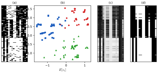
28.3.5.1 Example: binary PCA
p. 957, (28.118)–(28.119) With \(p(\bm x\given\bm z)=\prod_d\mathrm{Ber}(x_d\given\sigma(\bm w_d^{\mathrm T}\bm z))\) (28.118), \(N=150\) bit vectors of length \(D=16\) are generated by choosing one of three binary prototypes and flipping bits at random (Figure 28.18a). Variational EM (Tipping 1998; the Jaakkola–Jordan bound, gap 20.12) with \(L=2\) gives a 2-d embedding \(\E[\bm z_n\given\bm x_n]\) in which the three groups separate, and the reconstruction probabilities \(p(\hat x_{nd}=1\given\bm x_n)=\int p(\bm z_n\given\bm x_n)\sigma(\bm w_d^{\mathrm T}\bm z_n)\,\d\bm z_n\) (28.119), thresholded at 0.5 (the MAP estimate), denoise the data. In my run 11.0% of the bits of the raw data differ from the generating prototype, and 1.0% of the thresholded reconstruction does; the variational lower bound rose from \(-1338\) to \(-1082\) (monotonically). The bound was confirmed to lie below the exact marginal log-likelihood in a one-dimensional latent case (quadrature).
28.3.5.2 Example: categorical PCA
p. 957, (28.120) The categorical generalisation \(p(\bm x\given\bm z)=\prod_d\mathrm{Cat}(x_d\given\mathrm{softmax}(\bm W_d\bm z))\) (28.120) is CatPCA, fitted by variational EM (Khan et al. 2010; the softmax has no conjugate bound as simple as the sigmoid's, so bounds are used). Its natural parameters are Gaussian, so \(\bm z\) is dense and can be negative, whereas in the Dirichlet model of Section 28.4.2 the mean parameters are linear in \(\bm z\).
28.3.6 Factor analysis with DNN likelihoods (VAEs)
pp. 957–958 Replace the linear decoder by a neural network, \(p(\bm x\given\bm z)=\N(\bm x\given f(\bm z;\bm\theta),\sigma^2\bm I)\) (28.121): "nonlinear FA" (or nonlinear exponential family FA for other likelihoods). Posterior and MLE are then intractable; the variational autoencoder fits it with amortised variational inference (Chapter 21; the linear VAE is PPCA, gap 21.5), though MCMC also works (Hoffman 2017).
28.3.7 Factor analysis with GP likelihoods (GP-LVM)
pp. 958–959, (28.122)–(28.127) In the GP-LVM (Lawrence 2005) the linear decoder is replaced by a Gaussian process, one per output dimension, with the observed variable written \(\bm y\) to match the GP notation. Starting from PPCA, \(\bm z_i\sim\N(\bm0,\bm I)\), \(\bm y_i\given\bm z_i\sim\N(\bm W\bm z_i,\sigma^2\bm I)\), one can integrate out \(\bm z\) and maximise over \(\bm W\) (the primal, solved by the eigenvectors of \(\bm Y^{\mathrm T}\bm Y\)), or put a prior \(p(\bm W)=\prod_j\N(\bm w_j\given\bm 0,\bm I)\), integrate out \(\bm W\) and maximise over \(\bm Z\) (the dual): \(p(\bm Y\given\bm Z,\sigma^2)=\prod_{d=1}^D\N(\bm Y_{:,d}\given\bm0,\bm Z\bm Z^{\mathrm T}+\sigma^2\bm I)\) (28.125). With a kernel \(K\) in place of the linear kernel \(\bm Z\bm Z^{\mathrm T}\), the MLE of \(\bm Z\) needs gradient-based optimisation; the book's Figure 28.19 embeds motion-capture poses.
Filling the gap 28.9: the dual of PPCA, and the closed-form optimum of the GP-LVM with a linear kernel pp. 958–959, (28.124)–(28.127)
Proof
Marginalising \(\bm W\) (28.125)–(28.126). For output dimension \(d\) write \(\bm y_{:,d}=\bm Z\bm w_d+\bm\epsilon_d\), with \(\bm w_d\sim\N(\bm0,\bm I_L)\) and \(\bm\epsilon_d\sim\N(\bm0,\sigma^2\bm I_N)\) independent, so \(\bm y_{:,d}\sim\N(\bm0,\bm Z\bm Z^{\mathrm T}+\sigma^2\bm I)\); different \(d\) are independent. Hence \(\log p(\bm Y\given\bm Z,\sigma^2)=-\frac{ND}2\log2\pi-\frac D2\log|\bm K_\sigma|-\frac12\mathrm{tr}(\bm K_\sigma^{-1}\bm Y\bm Y^{\mathrm T})\) with \(\bm K_\sigma=\bm Z\bm Z^{\mathrm T}+\sigma^2\bm I\) (the determinant in (28.126) is \(|\bm K_\sigma|\), not \(|\bm K_z|\)). With a general Mercer kernel \(\bm K_\sigma=\bm K(\bm Z,\bm Z)+\sigma^2\bm I\) this is a product of independent GP marginal likelihoods sharing the inputs \(\bm Z\), and its gradient with respect to \(\bm K_\sigma\) is \(\frac12(\bm K_\sigma^{-1}\bm Y\bm Y^{\mathrm T}\bm K_\sigma^{-1}-D\bm K_\sigma^{-1})\), the same formula as in gap 18.22, followed by the chain rule through the kernel to \(\bm Z\) and the hyper-parameters.
The linear kernel is PPCA with the roles of \(N\) and \(D\) exchanged. Divide by \(D\) and put \(\bm S'=\frac1D\bm Y\bm Y^{\mathrm T}\) (an \(N\times N\) matrix): \(\frac2D\log p=-\big[\log|\bm K_\sigma|+\mathrm{tr}(\bm K_\sigma^{-1}\bm S')\big]+\mathrm{const}\). This has exactly the form of the PPCA objective (28.66), \(-[\log|\bm C|+\mathrm{tr}(\bm C^{-1}\bm S)]\), with \(\bm C=\bm W\bm W^{\mathrm T}+\sigma^2\bm I\) and \(\bm S\) a covariance, with \(\bm W\) replaced by \(\bm Z\) and \(\bm S\) by \(\bm S'\). The PPCA theorem (gap 20.7) therefore applies: for fixed \(\sigma^2\) the maximiser over \(\bm Z\) is \[ \hat{\bm Z}=\bm U_Q(\bm\Lambda_Q-\sigma^2\bm I)^{1/2}\bm R,\qquad\bm S'=\bm U\bm\Lambda\bm U^{\mathrm T}, \] with \(\bm U_Q\) the leading \(Q\) eigenvectors of \(\bm S'=\frac1D\bm Y\bm Y^{\mathrm T}\) and \(\bm R\) orthogonal. Because \(\bm Y\bm Y^{\mathrm T}\) and \(\bm Y^{\mathrm T}\bm Y\) share their non-zero eigenvalues and their eigenvectors are related by \(\bm Y\), \(\hat{\bm Z}\) spans the same principal subspace as the PPCA scores: the dual solves the same problem. I confirmed numerically for a random data set (\(N=40\), \(D=12\), \(Q=2\), \(\sigma=0.3\)) that the gradient of \(\log p(\bm Y\given\bm Z,\sigma^2)\) at \(\hat{\bm Z}\) vanishes to \(6\times10^{-12}\) and that 300 random perturbations of \(\hat{\bm Z}\) all lower the likelihood.
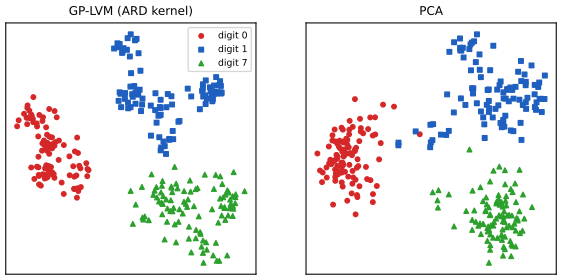
The advantage of the dual is the kernel: "factor analysis is linear regression with unknown inputs, the GP-LVM is GP regression with unknown inputs". The likelihood is multimodal in \(\bm Z\) for a nonlinear kernel; the usual start is the PCA solution.
28.4 LFMs with non-Gaussian priors
pp. 959–963 Table 28.1 lists the linear latent factor models with non-Gaussian priors that this section and the next two treat: NMF, multinomial PCA, LDA, ICA and sparse coding.
28.4.1 Non-negative matrix factorization (NMF)
pp. 960–961, (28.128) A gamma prior on the latents, \(p(\bm z)=\prod_k\mathrm{Ga}(z_k\given\alpha_k,\beta_k)\), gives a sparse, non-negative code, useful for sparse non-negative data such as word counts, where a Poisson likelihood \(p(\bm x\given\bm z)=\prod_d\mathrm{Poi}(x_d\given\bm w_d^{\mathrm T}\bm z)\) is natural: the gamma-Poisson (GaP) model (Canny 2004), \(p(\bm z,\bm x)=\prod_k\mathrm{Ga}(z_k\given\alpha_k,\beta_k)\prod_d\mathrm{Poi}(x_d\given\bm w_d^{\mathrm T}\bm z)\) (28.128). The parameters \(\alpha_k,\beta_k\) control the sparsity of \(\bm z\), and the book states that setting \(\alpha_k=\beta_k=0\) and computing the MLE of \(\bm W\) recovers non-negative matrix factorisation (Paatero and Tapper 1994; Lee and Seung 1999, 2001) as shown by Buntine and Jakulin (2006).
Filling the gap 28.10: NMF is maximum likelihood (EM) for a Poisson factor model, the multiplicative updates, and what the gamma prior adds p. 960, (28.128)
Proof
Superposition. If \(s_{ndk}\sim\mathrm{Poi}(z_{nk}w_{kd})\) are independent and \(x_{nd}=\sum_ks_{ndk}\), then \(x_{nd}\sim\mathrm{Poi}(\sum_kz_{nk}w_{kd})\), the sum of independent Poissons being Poisson with the summed rate, and given \(x_{nd}\) the vector \((s_{ndk})_k\) is multinomial with total \(x_{nd}\) and probabilities \(z_{nk}w_{kd}/\sum_jz_{nj}w_{jd}\) (the conditional of independent Poissons given their sum). This is the latent-variable form of the GaP likelihood with \(\bm W\) now \(K\times D\) and \(\bm Z\) the \(N\times K\) matrix of codes.
Equivalence with the KL divergence. The log-likelihood of the data matrix under rates \(m_{nd}=(\bm Z\bm W)_{nd}\) is \(\sum_{nd}[x_{nd}\log m_{nd}-m_{nd}-\log x_{nd}!]=-\sum_{nd}\big[x_{nd}\log\frac{x_{nd}}{m_{nd}}-x_{nd}+m_{nd}\big]+\sum_{nd}[x_{nd}\log x_{nd}-x_{nd}-\log x_{nd}!]\): the negative generalised KL divergence between \(\bm X\) and \(\bm Z\bm W\), plus a constant that does not involve the parameters. Maximum likelihood for \((\bm Z,\bm W)\) is therefore NMF with the KL (Lee–Seung) objective, over non-negative \(\bm Z,\bm W\).
EM and the multiplicative updates. E step: \(\E[s_{ndk}\given x_{nd}]=x_{nd}\,z_{nk}w_{kd}/m_{nd}\). The expected complete-data log-likelihood is \(\sum_{ndk}[\E s_{ndk}\log(z_{nk}w_{kd})-z_{nk}w_{kd}]+\mathrm{const}\). M step: setting the derivative in \(z_{nk}\) to zero gives \(z_{nk}=\sum_d\E s_{ndk}/\sum_dw_{kd}\), and in \(w_{kd}\), \(w_{kd}=\sum_n\E s_{ndk}/\sum_nz_{nk}\). Substituting the E step, \[ z_{nk}\leftarrow z_{nk}\,\frac{\sum_dw_{kd}\,x_{nd}/m_{nd}}{\sum_dw_{kd}},\qquad w_{kd}\leftarrow w_{kd}\,\frac{\sum_nz_{nk}\,x_{nd}/m_{nd}}{\sum_nz_{nk}}, \] the multiplicative updates of Lee and Seung (2001), which keep non-negativity automatically. EM never decreases the likelihood, so the divergence never increases (a fact that Lee and Seung proved by an auxiliary-function argument). My implementation (the updates applied alternately to \(\bm Z\) and \(\bm W\), each an EM step for a block) lowered the divergence monotonically (from 809.6 to 421.3 on a simulated Poisson matrix) and reached the same value as the library routine with the KL loss (419.9).
The gamma prior. With \(p(z_{nk})=\mathrm{Ga}(\alpha,\beta)\propto z^{\alpha-1}e^{-\beta z}\), the MAP-EM M step becomes \(z_{nk}=(\alpha-1+\sum_d\E s_{ndk})/(\beta+\sum_dw_{kd})\): the prior adds the pseudo-counts \(\alpha-1\) to the expected counts and the rate \(\beta\) to the exposure. With \(\alpha=1,\beta=0\) (a flat prior) MAP is NMF exactly. The improper prior \(\alpha=\beta=0\), \(p(z)\propto1/z\), has a MAP objective that is unbounded below as \(z\to0\), so I could not make the book's statement exact in that form; what holds is that the likelihood alone (no prior on \(\bm Z\)) is NMF, and the gamma prior shrinks the codes towards small, sparse values when \(\alpha<1\).
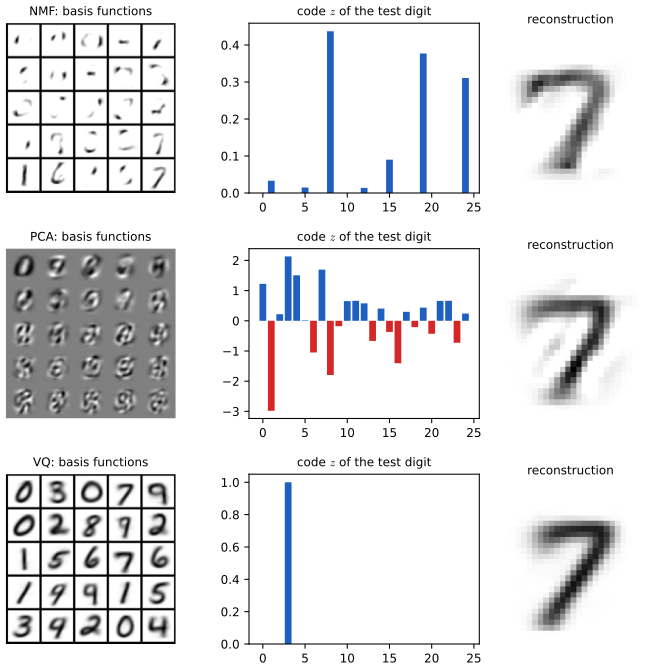
p. 961, Figure 28.21 Figure 28.21 compares NMF, vector quantisation (VQ, the GMM or K-means with one-hot code) and PCA as latent factor models for images: NMF learns small localised parts with a sparse, positive code; PCA learns global basis functions with a dense code of both signs; VQ learns whole prototypes with a one-hot code. The reconstruction quality is similar, the representations are very different.
28.4.2 Multinomial PCA
pp. 961–963, (28.129)–(28.130) With a Dirichlet prior \(\bm z\sim\mathrm{Dir}(\bm\alpha)\), \(\bm z\in\mathcal S_K\) (the probability simplex), \(\bm z\) is again sparse and non-negative but now sums to 1, and with categorical data \(x_d\in\{1,\dots,V\}\) and \(p(\bm x\given\bm z)=\prod_d\mathrm{Cat}(x_d\given\bm W_d\bm z)\) the model is \(p(\bm z,\bm x)=\mathrm{Dir}(\bm z\given\bm\alpha)\prod_d\mathrm{Cat}(x_d\given\bm W_d\bm z)\) (28.129). It goes by many names: the user rating profile model (Marlin 2003), the admixture model (Pritchard et al. 2000), the mixed membership model (Erosheva et al. 2004), multinomial PCA (Buntine and Jakulin 2006) and simplex factor analysis (Bhattacharya and Dunson 2011).
Roll-call example (28.4.2.1). Buntine and Jakulin fitted the model with five latent factors to the 2003 US Senate roll calls (\(x_{nd}\in\{+1,-1,0\}\) for 100 senators and 459 bills, with the outcome of each bill as a 101st "senator"); \(\E[z_{nk}\given\bm x_n]\) is the degree to which senator \(n\) belongs to "bloc" \(k\), and the blocs found include the Democratic and the Republican majorities (Figure 28.22). I cannot reproduce it: the data are not available.
Why a Dirichlet and not a Gaussian (28.4.2.2). The mean parameters \(p(x_{nd}=v\given\bm z_n)=\sum_kz_{nk}w^d_{vk}\) (28.130) are a convex combination of the columns of \(\bm W_d\): the latent variables combine additively in probability space, which aids interpretability. In CatPCA (Section 28.3.5.2) the linear predictor \(\bm W_d\bm z_n\) can be negative and must be passed through a softmax, so \(\bm z_n\) acts on log-odds and is harder to read. Connection to mixtures (28.4.2.3). If \(\bm z_n\) were one-hot, selecting a single column of \(\bm W_d\), the model would be a finite mixture of categoricals (Section 28.2.2), "all of \(\bm x\) comes from one cluster"; mPCA lets \(\bm z\) be any point of the simplex, so \(\bm x_n\) partially belongs to several clusters.
28.5 Topic models
p. 963 A topic model modifies mPCA for sequences of discrete tokens (words in documents, genes in DNA): the tokens are conditionally independent given a document-level topic vector \(\bm z\), which is a distribution over clusters, and each token is drawn from its own "local" cluster.
28.5.1 Latent Dirichlet allocation (LDA)
pp. 963–967 Latent Dirichlet allocation (Blei et al. 2003; in genetics the same model is the admixture model) is the most common topic model (not to be confused with linear discriminant analysis).
28.5.1.1 Model definition
Let \(x_{nl}\in\{1,\dots,V\}\) be the \(l\)-th word of document \(n\) (\(l=1,\dots,L_n\)), \(\bm z_n\sim\mathrm{Dir}(\bm\alpha)\) the topic proportions and \(w_{kv}\) the probability of word \(v\) in topic \(k\) (row \(\bm w_k=\bm W[k,:]\)): \(p(x_{nl}=v\given\bm z_n)=\sum_kz_{nk}w_{kv}\) (28.131). Introducing a topic indicator \(m_{nl}\in\{1,\dots,K\}\) per word, \(p(m_{nl}\given\bm z_n)=\mathrm{Cat}(\bm z_n)\), the joint is \[ p(\bm x_n,\bm z_n,\bm m_n)=\mathrm{Dir}(\bm z_n\given\bm\alpha)\prod_{l=1}^{L_n}\mathrm{Cat}(m_{nl}\given\bm z_n)\,\mathrm{Cat}(x_{nl}\given\bm W[m_{nl},:]) \tag{28.132} \] (Figure 28.23), with a prior \(\bm w_k\sim\mathrm{Dir}(\beta\bm 1_V)\) on topics. A small \(\beta\) makes each topic predict only a subset of the words; a small \(\alpha\) makes each document use only a few topics (Figure 28.24). Probabilistic LSA (Hofmann 1999) has the same likelihood but no prior on \(\bm z\), so it analyses a fixed corpus rather than being a generative model. The word-level view and the count-based view of the same model are reconciled in the next gap box.
Filling the gap 28.11: the word marginal, the count likelihood, and the Dirichlet facts used by LDA pp. 963–964, (28.131)–(28.132)
Proof
(28.131). Summing out the topic indicator, \(p(x_{nl}=v\given\bm z_n)=\sum_kp(m_{nl}=k\given\bm z_n)p(x_{nl}=v\given m_{nl}=k)=\sum_kz_{nk}w_{kv}\): the word distribution of the document is the convex combination \(\bm p_n=\bm W^{\mathrm T}\bm z_n\) of the topics. (Checked by simulation: the empirical word frequencies for \(\bm z=(0.5,0.3,0.2)\) match \(\bm z^{\mathrm T}\bm W\) to 0.01.)
Counts are enough. Given \(\bm z_n\), the words of a document are i.i.d. from \(\bm p_n\), so the probability of a particular word sequence depends only on the count vector \(\bm c_n=(c_{n1},\dots,c_{nV})\), \(c_{nv}=\sum_l\mathbb 1(x_{nl}=v)\), through \(\prod_vp_{nv}^{c_{nv}}\), and the counts are multinomial: \(\bm c_n\given\bm z_n\sim\mathrm{Mult}(L_n,\bm W^{\mathrm T}\bm z_n)\). Hence LDA is multinomial PCA (28.129) applied to word counts, with \(\bm z_n\) and the topics unchanged; the bag-of-words assumption (exchangeability within a document) is what makes the sequence information irrelevant. The word-level indicators \(m_{nl}\) are auxiliary variables, which is why the supplement can work with counts (the "count version" of variational inference), saving the \(O(\sum_nL_nVK)\) memory for the per-token responsibilities.
The Dirichlet. \(\mathrm{Dir}(\bm\alpha)\) has mean \(\bm\alpha/\alpha_0\) and, with \(\alpha_0=\sum_k\alpha_k\), covariance \(\mathrm{cov}(z_i,z_j)=\big(\alpha_i\alpha_0\delta_{ij}-\alpha_i\alpha_j\big)/\big(\alpha_0^2(\alpha_0+1)\big)\) (gap 2.6; confirmed by simulation). The marginal of one component is \(\mathrm{Beta}(\alpha_k,\alpha_0-\alpha_k)\); for the symmetric \(\alpha\bm1\) with \(\alpha<1\), the density piles up near the corners and edges of the simplex (U-shaped marginals), which is the sense in which small \(\alpha\) (or \(\beta\)) gives sparse topic proportions (or sparse topics).
pLSA and NMF. The pLSA likelihood \(\prod_{nv}(\bm z_n^{\mathrm T}\bm w_{:v})^{c_{nv}}\) is, up to the normalisation constraints on \(\bm z_n\) and \(\bm w_k\), the multinomial analogue of the Poisson likelihood of gap 28.10, and its EM algorithm is the corresponding normalised multiplicative update (Gaussier and Goutte 2005).
28.5.1.2 Polysemy
pp. 965–966, Figures 28.25–28.26 Each topic is a distribution over words that co-occur, so related words share topics; Figure 28.25 shows three topics learned from the TASA educational corpus (37,651 documents; 12 million tokens) that correspond to three senses of "play" (music, theatre, sports). Using the posterior \(\arg\max_kp(m_{nl}=k\given\bm x_n)\) the model assigns each occurrence of "play" to the sense indicated by the other words in the document (Figure 28.26: "music", "piano" push "play" to the musical topic): polysemy is resolved by the document-level topic distribution. Neither figure can be reproduced here (corpus unavailable); the 20 newsgroups topics of Figure S28.3 below show topics of the same kind (for example "space, launch, satellite, nasa, orbit, shuttle, earth"; "image, graphics, jpeg, software, file, gif"; "year, game, good, team, hit, players, runs"; "medical, health, patients, disease, doctor, cancer"), together with a topic of generic chatty words).
28.5.1.3 Posterior inference
pp. 966–967 Approximate posterior inference algorithms for LDA include mean-field variational inference (Blei et al. 2003), stochastic variational inference (Hoffman et al. 2010), collapsed Gibbs sampling (Griffiths and Steyvers 2004) and amortised inference networks (Miao et al. 2016; Srivastava and Sutton 2017); the supplement derives the first three, in the next subsection. There are also spectral methods with provable guarantees under an "anchor word" assumption (Arora et al. 2013). Number of topics (28.5.1.4): annealed importance sampling for the evidence (Wallach et al. 2009), held-out likelihood by cross-validation, the variational lower bound, or nonparametric Bayes (Teh et al. 2006; the Dirichlet process is in the nonparametric course).
S28.1 Inference in topic models supplement
Supplement, pp. 213–218 The supplement gives the two inference algorithms in detail. Write \(w_{k,v}\) for the topic-word probabilities, \(\pi_i\) for the topic proportions of document \(i\) (the main text's \(\bm z_n\)), and \(m_{il}\) for the topic of token \(l\) of document \(i\); \(\alpha\) and \(\gamma\) or \(\beta\) are the symmetric Dirichlet parameters.
S28.1.1 Collapsed Gibbs sampling for LDA
The uncollapsed Gibbs sampler draws \(m_{il}\) with \(p(m_{il}=k\given\cdot)\propto\exp[\log\pi_{ik}+\log w_{k,x_{il}}]\) S(28.1), \(\bm\pi_i\sim\mathrm{Dir}(\{\alpha_k+\sum_l\mathbb I(m_{il}=k)\})\) S(28.2) and \(\bm w_k\sim\mathrm{Dir}(\{\gamma_v+\sum_i\sum_l\mathbb I(x_{il}=v,m_{il}=k)\})\) S(28.3). Better mixing is obtained by integrating out all \(\bm\pi_i\) and \(\bm w_k\) (Griffiths and Steyvers 2004) and sampling only the discrete \(m_{il}\). Define \(N_{ivk}=\sum_l\mathbb I(m_{il}=k,x_{il}=v)\), \(N_{ik}=\sum_vN_{ivk}\), \(N_{vk}=\sum_iN_{ivk}\), \(N_k=\sum_vN_{vk}\) and \(L_i=\sum_kN_{ik}\). The marginal priors are \[ p(\bm m\given\alpha)=\Big(\frac{\Gamma(K\alpha)}{\Gamma(\alpha)^K}\Big)^N\prod_{i=1}^N\frac{\prod_{k=1}^K\Gamma(N_{ik}+\alpha)}{\Gamma(L_i+K\alpha)},\qquad p(\bm x\given\bm m,\beta)=\Big(\frac{\Gamma(V\beta)}{\Gamma(\beta)^V}\Big)^K\prod_{k=1}^K\frac{\prod_{v=1}^V\Gamma(N_{vk}+\beta)}{\Gamma(N_k+V\beta)} \tag{S28.5, S28.7} \] and the full conditional is \[ p(m_{il}=k\given\bm m_{-i,l},\bm x,\alpha,\beta)\propto\frac{N^-_{vk}+\beta}{N^-_k+V\beta}\cdot\frac{N^-_{ik}+\alpha}{L_i+K\alpha}\qquad(x_{il}=v), \tag{S28.8} \] where the superscript \(-\) means the counts computed without token \((i,l)\). A token is assigned to a topic according to how often the topic generates that word (first factor) and how much the topic is used in that document (second).
Filling the gap 28.12: the collapsed marginals and the full conditional of collapsed Gibbs sampling Supplement pp. 213–214, S(28.4)–S(28.8)
Proof
The marginal over \(\bm m\). For one document, with \(\bm\pi\sim\mathrm{Dir}(\alpha\bm1_K)\), the topic indicators are conditionally i.i.d. \(\mathrm{Cat}(\bm\pi)\), so \[ \int\prod_{l=1}^{L}\pi_{m_l}\,\frac{\Gamma(K\alpha)}{\Gamma(\alpha)^K}\prod_k\pi_k^{\alpha-1}\,\d\bm\pi=\frac{\Gamma(K\alpha)}{\Gamma(\alpha)^K}\int\prod_k\pi_k^{N_k+\alpha-1}\d\bm\pi=\frac{\Gamma(K\alpha)}{\Gamma(\alpha)^K}\frac{\prod_k\Gamma(N_k+\alpha)}{\Gamma(L+K\alpha)}, \] by the Dirichlet normaliser \(\int\prod_k\pi_k^{a_k-1}=\prod_k\Gamma(a_k)/\Gamma(\sum_ka_k)\) with \(a_k=N_k+\alpha\) and \(\sum_ka_k=L+K\alpha\). Independent documents multiply: S(28.5). (For \(K=2\), \(L=8\), counts \((3,5)\), \(\alpha=0.5\) the value \(-6.5905\) agrees with a direct numerical integral to \(10^{-3}\).) The same computation for each topic, with the \(V\)-dimensional \(\bm w_k\sim\mathrm{Dir}(\beta\bm1_V)\) and the words assigned to topic \(k\), gives S(28.7).
The conditional. \(p(m_{il}=k\given\bm m_{-i,l},\bm x)\propto p(\bm x,\bm m)\) as a function of \(k\) with the other assignments fixed. Compare the counts with token \((i,l)\) assigned to \(k\) against the counts without it: in S(28.5) only the document-\(i\) factor changes, \(\Gamma(N_{ik}^-+\alpha+1)/\Gamma(N_{ik}^-+\alpha)=N_{ik}^-+\alpha\) (using \(\Gamma(x+1)=x\Gamma(x)\)), while the denominator \(\Gamma(L_i+K\alpha)\) does not depend on \(k\); in S(28.7) only topic \(k\) changes, \(\Gamma(N^-_{vk}+\beta+1)/\Gamma(N^-_{vk}+\beta)=N^-_{vk}+\beta\) and \(\Gamma(N^-_k+V\beta+1)/\Gamma(N_k^-+V\beta)=N_k^-+V\beta\) in the denominator. Multiplying the ratios gives S(28.8). (The denominator \(L_i+K\alpha\) in the book is the same for every \(k\), and could be \(L_i-1+K\alpha\) if the token is removed first; it cancels on normalisation.) I confirmed numerically that (S28.8) equals the ratio of the collapsed joints \(p(\bm x,\bm m)\) with the token assigned to each topic, to \(10^{-10}\).
The sampler and its estimates. Initialise the \(m_{il}\) at random, then repeatedly: remove the token's counts, draw a new topic from S(28.8), add the counts back. The posterior mean of the topic-word probabilities from one sample is \(\hat w_{kv}=(N_{vk}+\beta)/(N_k+V\beta)\) (the mean of the Dirichlet posterior given the assignments), and similarly \(\hat\pi_{ik}=(N_{ik}+\alpha)/(L_i+K\alpha)\). The log of the collapsed joint rises during sampling (from \(-374.8\) to \(-283.7\) in the example of Figure S28.2), and the topic labels are only identified up to permutation: label switching (Section 28.2.6).
Figure S28.2 uses the supplement's example: 16 short documents over five words, with topic 1 uniform on {money, loan, bank} and topic 2 uniform on {river, stream, bank}. After 64 sweeps the sampler has assigned most tokens to their generating topic, in particular the ambiguous word "bank" is assigned according to the other words of its document. My run (\(\alpha=\beta=0.5\), documents of 8 to 15 tokens drawn with \(\bm\pi_i\sim\mathrm{Dir}(0.4,0.4)\)) gives the estimates \(\hat p(\text{money},\text{loan},\text{bank}\given k{=}1)=(0.35,0.40,0.23)\) and \(\hat p(\text{river},\text{stream},\text{bank}\given k{=}2)=(0.23,0.30,0.42)\), against \(1/3\) each; the other two entries are \(0.01\) to \(0.03\).
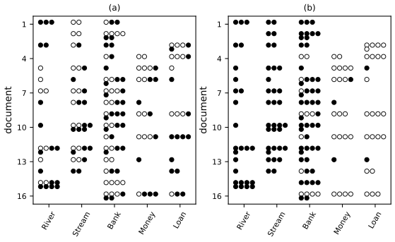
S28.1.2 Variational inference for LDA
A faster alternative is variational EM (the general scheme is in gap 10.11). Sequence version (S28.1.2.1). Use a fully factorised \(q(\bm z_n,\bm s_n)=\mathrm{Dir}(\bm z_n\given\tilde{\bm z}_n)\prod_l\mathrm{Cat}(\bm s_{nl}\given\tilde{\bm N}_{nl})\) (S28.9) (the supplement writes \(\bm s_{nl}\) for the topic indicator, \(m_{nl}\) in the main text): \(\tilde N_{nlk}\propto w_{d,k}\exp(\E[\log z_{nk}])\) for \(d=x_{nl}\), with \(\E[\log z_{nk}]=\psi(\tilde z_{nk})-\psi(\sum_{k'}\tilde z_{nk'})\) (S28.10)–(S28.11), \(\tilde z_{nk}=\alpha_k+\sum_l\tilde N_{nlk}\) (S28.12) and the M step \(\hat w_{dk}\propto\beta_d+\sum_n\sum_l\tilde N_{nlk}\mathbb I(x_{nl}=d)\) (S28.13). Count version (S28.1.2.2). Work with counts \(x_{nd}=\sum_l\mathbb I(x_{nl}=d)\) and \(q(\bm z_n,\bm N_n)=\mathrm{Dir}(\bm z_n\given\tilde{\bm z}_n)\prod_d\mathcal M(\bm N_{nd}\given x_{nd},\tilde{\bm N}_{nd})\) (S28.14): \(\tilde z_{nk}=\alpha_k+\sum_dx_{nd}\tilde N_{ndk}\), \(\tilde N_{ndk}\propto w_{dk}\exp(\E\log z_{nk})\), \(\hat w_{dk}\propto\beta_d+\sum_nx_{nd}\tilde N_{ndk}\) (S28.15)–(S28.17), with memory \(O(NV K)\) instead of \(O(\sum_nL_nVK)\). Bayesian version (S28.1.2.3). Giving \(\bm W\) a variational Dirichlet \(q(\bm w_k)=\mathrm{Dir}(\tilde{\bm w}_k)\) too (variational Bayes) changes only \(\tilde N_{ndk}\propto\exp(\E[\log w_{dk}]+\E[\log z_{nk}])\) (S28.19); the M step becomes a pseudo-count update \(\tilde w_{dk}=\beta_d+\sum_nx_{nd}\tilde N_{ndk}\) (S28.20), and \(\beta\ll1\) encourages sparse topics (Section 10.3.6.6 of the book). Algorithm S28.1 (batch VB for LDA) initialises \(\tilde{\bm W}\) by EM for a multinomial mixture and iterates the E step over all documents and the M step; Algorithm S28.2 is the online version.
Filling the gap 28.13: the mean-field updates of LDA and why they are coordinate ascent on the ELBO Supplement pp. 215–217, S(28.9)–S(28.20), Algorithm S28.1
Proof
Use the document-level model \(p(\bm z,\bm m,\bm x\given\bm W)=\mathrm{Dir}(\bm z\given\bm\alpha)\prod_l z_{m_l}w_{m_l,x_l}\), and \(q=q(\bm z)\prod_lq(m_l)\). The mean-field coordinate update is \(\log q(\cdot)=\E_{q(\mathrm{rest})}[\log p]+\mathrm{const}\) (gap 10.11).
The update of \(q(m_l)\). The terms of \(\log p\) involving \(m_l\) are \(\log z_{m_l}+\log w_{m_l,x_l}\); the expectation over \(q(\bm z)\) replaces \(\log z_k\) by \(\E_q[\log z_k]\), so \(q(m_l=k)\propto w_{k,x_l}\exp(\E[\log z_k])\). For a Dirichlet \(\mathrm{Dir}(\bm\gamma)\), \(\E[\log z_k]=\psi(\gamma_k)-\psi(\sum_{k'}\gamma_{k'})\): differentiate \(\log\int\prod_kz_k^{\gamma_k-1}\d\bm z=\sum_k\log\Gamma(\gamma_k)-\log\Gamma(\sum\gamma)\) with respect to \(\gamma_k\) (the derivative of the log-normaliser of an exponential family is the expectation of the sufficient statistic \(\log z_k\)). S(28.10)–S(28.11) follow.
The update of \(q(\bm z)\). The terms involving \(\bm z\) are \((\alpha_k-1)\log z_k+\sum_l\mathbb I(m_l=k)\log z_k\); taking the expectation under \(q(m_l)=\tilde N_{lk}\) gives \(\log q(\bm z)=\sum_k(\alpha_k+\sum_l\tilde N_{lk}-1)\log z_k\), a Dirichlet with \(\tilde z_k=\alpha_k+\sum_l\tilde N_{lk}\): S(28.12), "adding up the expected counts".
The count version. All tokens with the same word \(d\) have the same update (the right-hand side of the \(q(m_l)\) update depends on \(l\) only through \(x_l=d\)), so \(\tilde N_{lk}=\tilde N_{dk}\) for these tokens, and the sum \(\sum_l\tilde N_{lk}\) equals \(\sum_dx_d\tilde N_{dk}\): S(28.15)–S(28.16) are S(28.10)–S(28.12) with the tokens grouped by word, and the \(O(\sum_nL_n\cdot K)\) per-token memory is reduced to \(O(V_nK)\) per document.
The M step (EM and VB). With a point estimate of \(\bm W\), maximising \(\sum_n\sum_dx_{nd}\sum_k\tilde N_{ndk}\log w_{dk}\) under \(\sum_dw_{dk}=1\) gives \(w_{dk}\propto\sum_nx_{nd}\tilde N_{ndk}\) (adding a Dirichlet\((\beta+1)\) prior adds \(\beta\); the supplement's \(\beta_d+\) is that MAP form). With a variational \(q(\bm w_k)\) the same coordinate argument as for \(\bm z\) gives \(q(\bm w_k)=\mathrm{Dir}(\beta+\sum_nx_{nd}\tilde N_{ndk})\), S(28.20), and the \(\bm W\) factor of S(28.19) uses \(\E[\log w_{dk}]\) by the digamma identity above.
Monotonicity and the evidence. Each update maximises the ELBO in one factor, so the bound never decreases. At the document level, with \(\bm W\) fixed, I confirmed numerically (\(K=2\), \(V=6\), four distinct words) that the ELBO increased at every iteration and stayed below the exact log evidence (\(-20.884\) against \(-19.988\), quadrature over \(z\in[0,1]\)), that the fixed point satisfies \(\gamma_k=\alpha+\sum_dx_d\phi_{dk}\) to \(10^{-5}\), and that batch VB (Algorithm S28.1, 25 iterations) and the library's batch variational LDA recover the topics of a synthetic corpus (300 documents) to a mean absolute error of \(0.0014\) and \(0.0013\).
S28.1.2.4 Online (SVI) version
In the batch version each mean-field pass costs \(O(NN_zN_w)\). Stochastic variational inference (Hoffman et al. 2010; gap 10.3) treats a single document \(n\) as if the whole data set consisted of \(N\) copies of it: it computes \(\tilde{\bm w}^{\rm new}_{dk}=\beta_d+Nx_{nd}\tilde N_{ndk}\) and moves \(\tilde{\bm W}\) a step of size \(\eta_t\) towards it, \(\tilde w_{dk}\leftarrow(1-\eta_t)\tilde w_{dk}+\eta_t\tilde w_{dk}^{\rm new}\) (Algorithm S28.2), with a decaying step size; in practice minibatches of 256 to 4096 documents are used. Supplement Figure S28.3 shows, on English Wikipedia, that the online algorithm reaches the same test perplexity in far fewer document visits.
Filling the gap 28.14: online variational Bayes is a natural-gradient step on the ELBO, and when it converges Supplement p. 217–218, Algorithm S28.2, Figure S28.3
Proof
The global variational parameters are the Dirichlet parameters \(\tilde{\bm W}=(\tilde w_{dk})\), and the ELBO with the document-level variables optimised out is \(\mathcal L(\tilde{\bm W})=\sum_n\ell_n(\tilde{\bm W})+\E_q[\log p(\bm W)/q(\bm W)]\). The \(\bm W\) factor of the model is a Dirichlet, a conjugate exponential-family prior for the (multinomial) complete-data likelihood, so for the exponential family \(q(\bm w_k)=\mathrm{Dir}(\tilde{\bm w}_k)\) the Euclidean gradient of \(\mathcal L\) in the natural parameters \(\tilde{\bm w}_k-1\) is \(\bm F(\tilde{\bm w}_k)(\hat{\bm w}_k-\tilde{\bm w}_k)\) with \(\bm F\) the Fisher information of \(q\) and \(\hat w_{dk}=\beta_d+\sum_nx_{nd}\tilde N_{ndk}\) the full-batch update, so the natural gradient is \(\hat{\bm w}_k-\tilde{\bm w}_k\) (the general result is gap 6.11 and Hoffman et al. 2013). A natural-gradient step of size \(\eta\) is \(\tilde{\bm w}\leftarrow\tilde{\bm w}+\eta(\hat{\bm w}-\tilde{\bm w})=(1-\eta)\tilde{\bm w}+\eta\hat{\bm w}\); with \(\eta=1\) it is the batch VB update (Algorithm S28.1). For a random document (or minibatch \(B\)) the estimate \(\hat w^{(B)}_{dk}=\beta_d+\frac N{|B|}\sum_{n\in B}x_{nd}\tilde N_{ndk}\) is unbiased for \(\hat w_{dk}\), which gives Algorithm S28.2 and shows that "treating the single document as if the data set had \(N\) copies of it" is exactly the \(N/|B|\) rescaling.
Convergence. The iteration is a Robbins–Monro stochastic approximation with step \(\eta_t\), which converges to a stationary point of the ELBO if \(\sum_t\eta_t=\infty\) and \(\sum_t\eta_t^2<\infty\); the schedule \(\eta_t=(\tau_0+t)^{-\kappa}\) satisfies both for \(\kappa\in(\frac12,1]\), the delay \(\tau_0\) down-weights the early, noisy iterations, and larger minibatches reduce the variance. In my experiment (20 newsgroups, six groups, 1500 training documents, 3000 words, \(K=20\), \(\alpha=0.1\), \(\beta=0.01\); held-out perplexity by document completion on 300 test documents) the batch algorithm reaches a perplexity of 2029, 1884 and 1788 after 1, 2 and 8 passes (12 000 document visits), while the online algorithm (minibatch 64, \(\kappa=0.7\), \(\tau_0=64\)) reaches 1803 after 1024 document visits and 1622 after 32 768; \(\kappa=0.6\) and \(\tau_0=16\) were clearly worse (1771, 1733). The online algorithm, which updates after every minibatch, ends at a lower perplexity than the batch one here; the book reports similar final perplexity at much lower cost on a corpus so large that the batch algorithm cannot afford many passes (Figure S28.3).
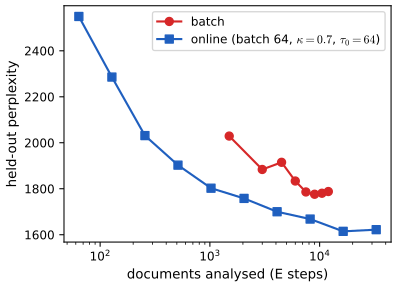
28.5.2 Correlated topic model
pp. 967–968, (28.133) LDA cannot represent correlations between topics ("business" co-occurring with "finance"), because the Dirichlet has a fixed covariance structure. The correlated topic model (Blei and Lafferty 2007) replaces it by the logistic normal distribution, \(p(\bm z)=\int\mathrm{Cat}(\bm z\given\mathrm{softmax}(\bm\epsilon))\N(\bm\epsilon\given\bm\mu,\bm\Sigma)\,\d\bm\epsilon\) (28.133) (here \(\bm z\) is a draw of the topic-proportion vector, \(\mathrm{softmax}(\bm\epsilon)\) itself). It differs from CatPCA (28.3.5.2) in where the Gaussian acts: the CTM models the mean parameters of the word distribution through \(x_{nl}\sim\mathrm{Cat}(\bm W^{\mathrm T}\mathrm{softmax}(\bm\epsilon_n))\) (so \(\bm z\) is sparse and non-negative), while CatPCA models the natural parameters, \(x_{nd}\sim\mathrm{Cat}(\mathrm{softmax}(\bm W_d\bm z_n))\) (dense, possibly negative). The prior is no longer conjugate to the multinomial, but a variational mean-field approximation exists (Blei and Lafferty 2007). After fitting one may prune weak entries of the precision \(\hat{\bm\Sigma}^{-1}\) to get a sparse Gaussian graphical model of topic dependencies (Figure 28.27, from Science articles 1990–1999, which is not reproducible here).
Filling the gap 28.15: why a Dirichlet cannot have positively correlated components p. 967
Proof
For \(\bm z\sim\mathrm{Dir}(\bm\alpha)\) with \(\alpha_0=\sum\alpha_k\): \(\mathrm{cov}(z_i,z_j)=-\alpha_i\alpha_j/\big(\alpha_0^2(\alpha_0+1)\big)\) for \(i\ne j\) (the book's "\(\Sigma_{ij}=-\alpha_i\alpha_j\)" omits the positive normalising factor), which is strictly negative for every \(\bm\alpha\). The reason is the constraint \(\sum_kz_k=1\): the covariance matrix of a Dirichlet is \(\frac1{\alpha_0+1}(\mathrm{diag}(\bar{\bm z})-\bar{\bm z}\bar{\bm z}^{\mathrm T})\) with \(\bar{\bm z}=\bm\alpha/\alpha_0\), so the only freedom is the mean \(\bar{\bm z}\) and the concentration \(\alpha_0\); the correlation between components \(i,j\) is \(-\sqrt{\bar z_i\bar z_j/((1-\bar z_i)(1-\bar z_j))}\), fixed by the means. A logistic normal \(\bm z=\mathrm{softmax}(\bm\epsilon)\), \(\bm\epsilon\sim\N(\bm\mu,\bm\Sigma)\), has a free \(K\times K\) covariance \(\bm\Sigma\) and so can place two topics together: for example for \(\epsilon_1,\epsilon_2\) strongly positively correlated, both proportions rise and fall together relative to a third topic. I confirmed the Dirichlet covariance formula by simulation (400 000 draws, error below \(2\times10^{-3}\)).
28.5.3 Dynamic topic model
pp. 967–969, (28.134)–(28.137) LDA assumes static topics. In the dynamic topic model (Blei and Lafferty 2006) the topic parameters follow a Gaussian random walk, \(\bm w^t_k\given\bm w^{t-1}_k\sim\N(\bm w^{t-1}_k,\sigma^2\bm I)\), mapped to probabilities by a softmax: \(\bm z^t_n\sim\mathrm{Dir}(\alpha\bm1)\), \(m^t_{nl}\given\bm z^t_n\sim\mathrm{Cat}(\bm z^t_n)\), \(x^t_{nl}\given m^t_{nl}=k\sim\mathrm{Cat}(\mathrm{softmax}(\bm w^t_k))\) (Figure 28.28). Inference uses structured mean field with the Kalman smoother on the Gaussian chain of each topic (Chapter 8); Figure 28.29 shows the "neuroscience" topic of the journal Science over 120 years drifting from "nerve" and "movement" towards "neuron", "cell", "channel" and "calcium receptor". The dynamic embedded topic model (Dieng et al. 2019) uses word embeddings and amortised inference to handle rare words. The corpus is not available, so I do not reproduce Figure 28.29.
28.5.4 LDA-HMM
pp. 969–971, (28.138)–(28.141) LDA treats words as exchangeable; an HMM models short-range word order but not the gist of a document. The LDA-HMM (Griffiths et al. 2004) combines them: for each document an HMM with states \(h_{nl}\in\{0,\dots,H\}\) chooses, at every position, whether the word comes from the semantic LDA model (state 0, with topic \(m_{nl}\)) or from a syntactic HMM state \(j>0\): \[ p(\bm z_n)=\mathrm{Dir}(\alpha\bm1),\ p(m_{nl}=k\given\bm z_n)=z_{nk},\ p(h_{nl}=j\given h_{n,l-1}=i)=A_{ij},\ p(x_{nl}=d\given m_{nl}=k,h_{nl}=j)=\begin{cases}W_{kd}&j=0\\B_{jd}&j>0\end{cases} \] (28.138)–(28.141), fitted by collapsed Gibbs sampling. With \(N_z=200\) topics and \(H=20\) states on the combined Brown and TASA corpora the HMM captures function words ("the", "of", "and", "to") and the LDA the content words; without it, the LDA topics are polluted by function words, which is why they are usually removed (Table 28.2). The model also disambiguates a word used syntactically or semantically, e.g. "return" as a verb or as a noun, or "graph" as an adjective-noun modifier or an object (Figure 28.31, NIPS corpus). Topic-RNN (Dieng et al. 2017) replaces the HMM by an RNN. These results need the corpora and are not reproduced.
28.6 Independent components analysis (ICA)
pp. 971–978 In a crowded room many people speak; your two ears act as two microphones that hear linear mixtures of the speech signals, and the goal is to unmix them. This is the cocktail party problem or blind source separation (BSS; "blind" means nothing is known about the sources), which also arises in EEG and MEG analysis, financial data, and any data in which latent sources are mixed linearly.
28.6.1 Noiseless ICA model
pp. 972–973, (28.142)–(28.144) Let \(\bm x_n\in\R^D\) be the observed sensor vector and \(\bm z_n\in\R^D\) the source vector (the same dimension), with \[ \bm x_n=\bm A\bm z_n,\qquad p(\bm z_n)=\prod_{j=1}^Dp_j(z_{nj}), \tag{28.142} \] where \(\bm A\) is an invertible \(D\times D\) mixing (generative) matrix, i.e. \(x_{nj}=\sum_iA_{ji}z_{ni}\) (the book's (28.143) has the indices of \(\bm A\) and \(\bm z\) interchanged: \(\sum_iA_{ij}z_{nj}\)). The prior is typically sparse so that only a few signals are active at a time. The model is noiseless, so the posterior of the sources is a point mass: \(p(\bm z_n\given\bm x_n,\bm A)=\delta(\bm z_n-\bm B\bm x_n)\) with the recognition matrix \(\bm B=\bm A^{-1}\) (28.144).
28.6.2 The need for non-Gaussian priors
pp. 973–975, (28.145)–(28.147) Centring \(\bm z\) (\(\E\bm z=\bm0\)) and absorbing a scale into \(\bm A\) (\(\mathrm{cov}\,\bm z=\bm I\)) gives \(\mathrm{cov}\,\bm x=\bm A\bm A^{\mathrm T}\), so the sources are uncorrelated unit-variance variables, as in factor analysis; uncorrelatedness cannot identify \(\bm A\) (the rotation problem of Section 28.3.1.6), so ICA needs an independent and non-Gaussian prior. For two independent uniform sources (Figure 28.33a) mixed by \(\bm A=0.3\begin{pmatrix}2&3\\2&1\end{pmatrix}\) (28.145) one observes Figure 28.33b. Full-rank PCA is the same model with a factored Gaussian prior; it whitens the data (Figure 28.33c, \(\mathrm{cov}\,\bm z=\bm I\)), which solves "half" of the problem (the linear subspace); what remains is a rotation, and there is no information in the symmetric Gaussian to choose the angle. A non-Gaussian prior supplies the angle (Figure 28.33d), up to a permutation of the indices and a sign. A super-Gaussian prior (heavy tails) is typical, such as the Laplace with unit variance, \(\log p(z)=-\sqrt2|z|-\log\sqrt2\) (28.146) (not differentiable at 0), or the logistic distribution with mean 0 and variance 1 (\(s=\sqrt3/\pi\)), \(\log p(z)=-2\log\cosh\big(\frac\pi{2\sqrt3}z\big)-\log\frac{4\sqrt3}\pi\) (28.147) (checked numerically: both integrate to 1 and have variance 1).
Filling the gap 28.16: when ICA is identifiable, and a caveat about the sign of the kurtosis pp. 973–975
Proof
Gaussian sources are not identifiable. If \(\bm z\sim\N(\bm0,\bm I)\) and \(\bm R\) is orthogonal then \(\bm R\bm z\sim\N(\bm0,\bm I)\) has the same independent-component structure, and \(\bm x=\bm A\bm z=(\bm A\bm R^{\mathrm T})(\bm R\bm z)\): the pairs \((\bm A,\bm z)\) and \((\bm A\bm R^{\mathrm T},\bm R\bm z)\) generate the same distribution of \(\bm x\). On whitened data the ICA objective with a Gaussian prior, \(\E\sum_j\frac12(\bm v_j^{\mathrm T}\bm x)^2=\frac D2\), is constant in the orthogonal \(\bm V\): nothing selects a rotation. A whitened Gaussian sample has an almost flat ICA objective in the rotation angle (Figure x28.2, panel "gauss": range 0.006 over all angles, against 0.057 for uniform sources; the residual wiggle is sampling noise in the fourth moments).
Non-Gaussian sources are identifiable up to scale and permutation (Comon 1994). Suppose the whitened data are \(\tilde{\bm x}=\bm Q\bm s\) with \(\bm Q\) orthogonal and independent unit-variance sources \(\bm s\), at most one of which is Gaussian, and that another representation exists: \(\bm z=\bm V\tilde{\bm x}=\bm G\bm s\), \(\bm G=\bm V\bm Q\) orthogonal, with independent components \(z_1,\dots,z_D\). By the Darmois–Skitovich theorem (1953; cited without proof), if two linear forms \(\sum_ig_{1i}s_i\) and \(\sum_ig_{2i}s_i\) of independent variables are independent, then every \(s_i\) with \(g_{1i}g_{2i}\ne0\) is Gaussian. Applying it to every pair of rows of \(\bm G\): each non-Gaussian source appears in at most one row; since the columns of an orthogonal matrix have unit norm, it appears in exactly one. If there are \(D-1\) or \(D\) non-Gaussian sources, \(D-1\) columns have a single non-zero entry in distinct rows, and the orthogonality of \(\bm G\) forces the last column to have one as well. So \(\bm G\) is a signed permutation matrix: the sources are recovered up to order and sign, and the recovered \(\bm A\) up to column permutation and sign, the claim of Section 28.6.2. Two Gaussian sources could be rotated into each other, so "at most one Gaussian" is necessary as well as sufficient.
The role of the prior, and a caveat. The model used for estimation need not be the true one. With the logistic prior (28.147) the expected negative log-likelihood of a rotation \(\bm R(\theta)\) of independent unit-variance sources behaves differently according to the kurtosis of the true sources. For Laplace (super-Gaussian) sources it is smallest at the true rotation (population values 2.746 at \(0^\circ\) and \(90^\circ\), 2.800 at \(45^\circ\)); for uniform (sub-Gaussian) sources the same objective is largest at the true rotation (2.944 at \(0^\circ\), 2.892 at \(45^\circ\)) and smallest at the mixtures. So maximum likelihood with a super-Gaussian prior is correct only for super-Gaussian sources; for sub-Gaussian sources one needs a sub-Gaussian prior, or a flexible one that adapts the sign (extended InfoMax), or a method that uses the absolute value of a contrast. The true rotation is a stationary point in both cases, which is why the fixed-point FastICA algorithm of gap 28.18 finds the sources of Figure 28.33 even though the objective is at a maximum (Amari error 0.045). Figure x28.2 shows both cases (the dashed red lines are the true angles).
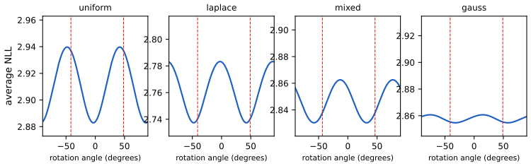
28.6.3 Maximum likelihood estimation
p. 975, (28.148)–(28.151) By the change of variables formula \(p_x(\bm x)=p_z(\bm z)|\det\bm A^{-1}|=p_z(\bm B\bm x)|\det\bm B|\) (28.148). Whiten the data first, \(\tilde{\bm x}=\bm S^{-1/2}\bm U^{\mathrm T}(\bm x-\bar{\bm x})\) with \(\bm\Sigma=\bm U\bm S\bm U^{\mathrm T}\), so that the unmixing matrix can be replaced by an orthogonal \(\bm V\) and \(|\det\bm V|=1\) is a constant (28.149). The average negative log-likelihood is then \[ \mathrm{NLL}(\bm V)=-\frac1N\sum_{j=1}^D\sum_{n=1}^N\log p_j(\bm v_j^{\mathrm T}\tilde{\bm x}_n)=\sum_j\E[G_j(z_j)],\qquad G_j=-\log p_j,\ z_j=\bm v_j^{\mathrm T}\tilde{\bm x}, \tag{28.150, 28.151} \] a non-convex objective to be minimised over orthogonal \(\bm V\). It can be minimised by projected gradient descent, or faster by the natural gradient (MacKay 2003, Ch. 34), but the most popular method is the approximate Newton method FastICA (Hyvärinen and Oja 2000), derived in gap 28.18 and used for Figure 28.32.
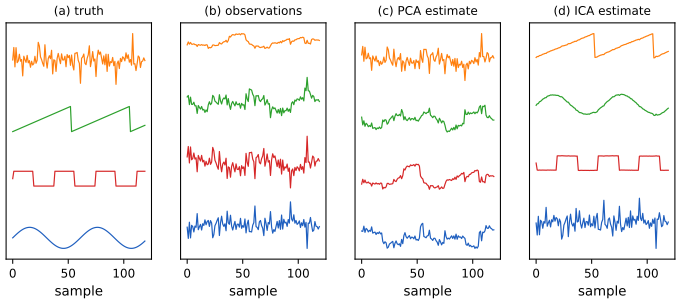
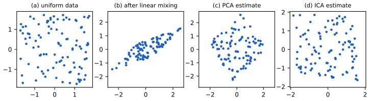
28.6.4 Alternatives to MLE
pp. 975–977 Three other classical estimators are, with a suitable choice of contrast, the same as maximum likelihood, and they give the problem its main interpretations. Maximising non-Gaussianity (28.6.4.1) (projection pursuit, Friedman and Tukey 1974) seeks \(\bm V\) so that \(\bm z=\bm V\tilde{\bm x}\) is as non-Gaussian as possible, measured by kurtosis (sensitive to outliers) or by negentropy \(\mathrm{negentropy}(z)=\mathbb H(\N(\mu,\sigma^2))-\mathbb H(z)\) (28.152) with \(\mu=\E z\), \(\sigma^2=\mathrm{var}\,z\), which is \(\ge0\) because the Gaussian maximises entropy at a fixed variance; the objective is \(J(\bm V)=\sum_j\mathrm{negentropy}(z_j)\) (28.153)=\(\sum_j-\mathbb H(z_j)+\mathrm{const}\) (28.154). Minimising total correlation (28.6.4.2): \(\mathrm{TC}(\bm z)=\sum_j\mathbb H(z_j)-\mathbb H(\bm z)=\Dkl(p(\bm z)\|\prod_jp(z_j))\) (28.155), zero iff the components are independent. Maximising mutual information, InfoMax (28.6.4.3) (Linsker 1988; Bell and Sejnowski 1995): maximise the information flow through the noisy encoder \(z_j=\phi(\bm v_j^{\mathrm T}\bm x)+\epsilon\), \(\epsilon\sim\N(0,1)\), whose \(I(\bm x;\bm z)=\mathbb H(\bm z)-\mathbb H(\bm z\given\bm x)\) has a constant second term, with \(\mathbb H(\bm z)\approx\sum_j\E\log\phi'(\bm v_j^{\mathrm T}\bm x)+\log|\det\bm V|\) (28.157); for \(\phi=\sigma\), \(\log\phi'(z)=-2\log\cosh(z/2)-\log4\), the logistic prior (28.147) up to constants. The book states that all of these are equivalent to the MLE; here is the exact statement.
Filling the gap 28.17: ML, negentropy, total correlation and InfoMax are one objective (exact identity) pp. 975–977, (28.150)–(28.157)
Proof
The identity. Let \(\tilde{\bm x}\) be the whitened data with density \(p_{\tilde x}\), \(\bm V\) orthogonal, \(\bm z=\bm V\tilde{\bm x}\) with density \(q\) and marginals \(q_j\), and let \(p_j\) be the model's source priors. Then \[ \mathrm{NLL}(\bm V)=\E\Big[-\sum_j\log p_j(z_j)\Big]=\sum_j\big[\mathbb H(q_j)+\Dkl(q_j\|p_j)\big]=\mathrm{TC}(\bm z)+\mathbb H(\bm z)+\sum_j\Dkl(q_j\|p_j), \] using \(\E[-\log p_j(z_j)]=\mathbb H(q_j)+\Dkl(q_j\|p_j)\) (cross-entropy decomposition) and \(\sum_j\mathbb H(q_j)=\mathrm{TC}(\bm z)+\mathbb H(\bm z)\) (28.155). Since \(\bm V\) is orthogonal, the map \(\tilde{\bm x}\mapsto\bm z\) has Jacobian determinant of absolute value 1, so \(\mathbb H(\bm z)=\mathbb H(\tilde{\bm x})\), which does not depend on \(\bm V\). Therefore \[ \mathrm{NLL}(\bm V)=\mathbb H(\tilde{\bm x})+\mathrm{TC}(\bm V\tilde{\bm x})+\sum_j\Dkl(q_j\|p_j). \] (I verified this on a two-dimensional two-component Gaussian-mixture density by two-dimensional quadrature: both sides equal 2.87282 at \(60^\circ\) to five digits.) The data entropy is a constant, so minimising the NLL is minimising total correlation (the dependence among the outputs) plus the mismatch between the marginals of the outputs and the model priors. If the prior family contains the true marginals, the second term is zero at the truth, and the minimum is \(\mathbb H(\tilde{\bm x})\) iff \(\mathrm{TC}=0\), i.e. \(\bm V\) separates the sources: population consistency of ICA by maximum likelihood.
Negentropy (28.152)–(28.154). With \(\E\bm z=\bm0\), \(\mathrm{cov}\,\bm z=\bm I\) (preserved by orthogonal \(\bm V\)) every \(\mathbb H(\N(0,1))\) is the constant \(\frac12\log(2\pi e)\), so \(J(\bm V)=\sum_j[\frac12\log2\pi e-\mathbb H(q_j)]=\mathrm{const}-\sum_j\mathbb H(q_j)\), and maximising \(J\) minimises \(\sum_j\mathbb H(q_j)=\mathrm{TC}+\mathbb H(\tilde{\bm x})\): negentropy maximisation is total-correlation minimisation exactly (28.6.4.2). It equals the NLL up to the mismatch term \(\sum_j\Dkl(q_j\|p_j)\), i.e. when the priors are (close to) the true marginals (the book writes \(\E\log p(z_j)\) in (28.154), which is \(-\mathbb H(q_j)\) only if \(p_j=q_j\)).
InfoMax (28.157). For the noiseless version \(z_j=\phi(\bm v_j^{\mathrm T}\tilde{\bm x})\) with monotone \(\phi\), \(\mathbb H(\bm z)=\mathbb H(\tilde{\bm x})+\E\log|\det\partial\bm z/\partial\tilde{\bm x}|=\mathbb H(\tilde{\bm x})+\sum_j\E\log\phi'(\bm v_j^{\mathrm T}\tilde{\bm x})+\log|\det\bm V|\), which is (28.157) (with the noisy encoder of the book it holds as an approximation when the noise is small relative to the signal). If \(\phi\) is the cdf of \(p_j\) then \(\phi'=p_j\) and maximising \(\mathbb H(\bm z)\) is maximising \(\sum_j\E\log p_j(\bm v_j^{\mathrm T}\tilde{\bm x})\), the log-likelihood. For \(\phi=\sigma\): \(\log\sigma'(z)=-z-2\log(1+e^{-z})=-2\log\cosh(z/2)-\log4\) (checked numerically), the logistic log-density up to the scale of \(z\), which is (28.147) up to constants.
Negentropy is non-negative for the standard cases: \(\frac12\log2\pi e=1.419\) exceeds the entropy of the unit-variance uniform, \(\log2\sqrt3=1.243\), Laplace, \(1+\log\sqrt2=1.347\), and logistic, \(2+\log(\sqrt3/\pi)=1.405\) (numerically verified).
Filling the gap 28.18: FastICA is an approximate Newton method on the contrast p. 975, Hyvärinen and Oja (2000)
Proof
One unit: maximise or minimise \(f(\bm w)=\E[G(\bm w^{\mathrm T}\tilde{\bm x})]\) subject to \(\|\bm w\|^2=1\), with \(g=G'\) and \(g'\) its derivative, over whitened data (\(\E\tilde{\bm x}=\bm0\), \(\E\tilde{\bm x}\tilde{\bm x}^{\mathrm T}=\bm I\)). The Lagrangian condition is \(F(\bm w)=\E[\tilde{\bm x}g(\bm w^{\mathrm T}\tilde{\bm x})]-\beta\bm w=\bm0\), with \(\beta=\E[\bm w^{\mathrm T}\tilde{\bm x}g(\bm w^{\mathrm T}\tilde{\bm x})]\) at the optimum (multiply by \(\bm w^{\mathrm T}\)). Newton's method for \(F(\bm w)=\bm0\) uses its Jacobian \(\E[\tilde{\bm x}\tilde{\bm x}^{\mathrm T}g'(\bm w^{\mathrm T}\tilde{\bm x})]-\beta\bm I\). The approximation of Hyvärinen: for whitened data \(\E[\tilde{\bm x}\tilde{\bm x}^{\mathrm T}g'(\bm w^{\mathrm T}\tilde{\bm x})]\approx\E[\tilde{\bm x}\tilde{\bm x}^{\mathrm T}]\E[g'(\bm w^{\mathrm T}\tilde{\bm x})]=\E[g']\bm I\) (the projection \(\bm w^{\mathrm T}\tilde{\bm x}\) is treated as approximately independent of \(\tilde{\bm x}\tilde{\bm x}^{\mathrm T}\)), so the Jacobian is the scalar matrix \((\E g'-\beta)\bm I\) and the Newton step is \(\bm w^+=\bm w-\frac{\E[\tilde{\bm x}g(\bm w^{\mathrm T}\tilde{\bm x})]-\beta\bm w}{\E g'-\beta}\). Multiplying by the scalar \((\beta-\E g')\) (which changes nothing after the normalisation of \(\bm w\) to unit length) \[ \bm w^+=\E[\tilde{\bm x}\,g(\bm w^{\mathrm T}\tilde{\bm x})]-\E[g'(\bm w^{\mathrm T}\tilde{\bm x})]\,\bm w,\qquad\bm w\leftarrow\bm w^+/\|\bm w^+\|, \] the FastICA step: no step size, and cubic convergence for the kurtosis nonlinearity when the sources have symmetric densities. For \(D\) components the rows \(\bm w_j\) are updated in parallel and then decorrelated by the symmetric orthogonalisation \(\bm W\leftarrow(\bm W\bm W^{\mathrm T})^{-1/2}\bm W\), the orthogonal matrix nearest to \(\bm W\) (this keeps all components on an equal footing); alternatively deflation orthogonalises each against the earlier ones. The choices \(g(u)=\tanh u\) (from \(G=\log\cosh\)) or \(g(u)=u^3\) (kurtosis) correspond to the logistic prior and to the kurtosis contrast. Since the iteration is a root-finding method for the stationarity condition it converges to any stationary point, a minimum or a maximum of \(f\) (see the caveat of gap 28.16). In my code FastICA unmixes four non-Gaussian sources with an Amari error of 0.012 (800 samples), agrees with the library implementation (both reach Amari errors between 0.01 and 0.03 on four-source mixtures of the kind in Figure 28.32), and identifies the uniform mixture of Figure 28.33 (Amari error 0.045 for \(N=300\), against 0.862 for whitening alone).
28.6.5 Sparse coding
pp. 977–978, (28.158)–(28.160) Allow observation noise and a non-square matrix \(\bm W\in\R^{D\times K}\) with a Laplace prior on the code: \[ p(\bm z,\bm x)=\prod_k\mathrm{Laplace}(z_k\given0,1/\lambda)\ \N(\bm x\given\bm W\bm z,\sigma^2\bm I). \tag{28.158} \] Each observation is a sparse combination of the columns of \(\bm W\) (basis functions); since few are active at a time, \(K\) may exceed \(D\), an overcomplete representation. For a batch \(\bm X\) (rows \(\bm x_n\)) the negative log joint is \(\frac1{2\sigma^2}\sum_n\|\bm x_n-\bm W\bm z_n\|^2+\lambda\|\bm z_n\|_1+\mathrm{const}\) (28.159)–(28.160). Inferring \(\bm Z\) for a fixed \(\bm W\) is sparse coding (an \(\ell_1\)-regularised least squares problem for each \(\bm x_n\), Section 15.2.6); learning \(\bm W\) is dictionary learning, difficult because \(\bm Z\) must be marginalised, so one usually optimises both jointly, alternating a sparse regression for \(\bm Z\) with a least-squares update of \(\bm W\) (Mairal et al. 2010 for faster algorithms). A neural network can be trained to approximate the \(\ell_1\) solution (predictive sparse decomposition, Kavukcuoglu et al. 2008). On natural image patches (centred, unit norm) the learned basis functions are bar and edge detectors resembling the simple cells of the primary visual cortex (Olshausen and Field 1996), whereas PCA yields sinusoidal gratings (Figure 28.34).
Filling the gap 28.19: MAP is the lasso, the scale ambiguity of (28.160), the alternating algorithm, and why PCA finds sinusoids pp. 977–978 and footnote 7
Proof
MAP. For fixed \(\bm W\), \(-\log p(\bm z\given\bm x)=\frac1{2\sigma^2}\|\bm x-\bm W\bm z\|^2+\lambda\|\bm z\|_1+\mathrm{const}\): the lasso (gap 15.9 derives it from the Laplace scale mixture), convex in \(\bm z\), with the optimality conditions \(\bm w_k^{\mathrm T}(\bm W\bm z-\bm x)/\sigma^2=-\lambda\,\mathrm{sign}(z_k)\) if \(z_k\ne0\) and \(|\bm w_k^{\mathrm T}(\bm W\bm z-\bm x)|/\sigma^2\le\lambda\) if \(z_k=0\). My FISTA solver (proximal gradient with momentum; soft-thresholding as the proximal map of \(\ell_1\)) satisfies them and agrees with the library coordinate-descent lasso to \(10^{-12}\) on a test problem.
The scale ambiguity. The objective (28.160) is not bounded in the useful way if both \(\bm W\) and \(\bm Z\) are free: replacing \((\bm W,\bm Z)\) by \((c\bm W,\bm Z/c)\) leaves the fit \(\bm W\bm Z\) unchanged and multiplies the penalty \(\lambda\|\bm Z\|_{1,1}\) by \(1/c\), so the infimum over \(c\to\infty\) is the unpenalised least-squares fit with no sparsity at all. (The joint optimisation therefore needs a constraint such as \(\|\bm w_k\|_2\le1\), as in dictionary learning, or a prior on \(\bm W\).) I confirmed the effect numerically: with \(c=100\) the penalty falls by a factor 100 at a constant fit. In my implementation the dictionary step is a least-squares solve followed by rescaling the columns to unit norm (and dead atoms are re-initialised), the code step is FISTA with warm starts; the objective decreased overall (0.2727 to 0.2630 on 600 patches, 12 outer iterations), and the final dictionaries have unit-norm columns.
Why PCA gives sinusoids (footnote 7). The covariance of patches from a stationary image is translation invariant: \(\mathrm{cov}[I(\bm r),I(\bm r')]=f(\|\bm r-\bm r'\|)\). On a periodic grid this is a (block) circulant matrix \(\bm C\) with first row \(\bm c\), and for \(\bm f_k=(1,\omega^k,\omega^{2k},\dots)/\sqrt n\), \(\omega=e^{2\pi i/n}\), \((\bm C\bm f_k)_j=\sum_lc_{l-j}\omega^{kl}/\sqrt n=\hat c_k\,(\bm f_k)_j\), so the Fourier modes are the eigenvectors, with eigenvalues the discrete Fourier transform \(\hat c_k\) of the covariance function (confirmed numerically for \(n=16\)); real combinations are sinusoids of different phases, and PCA ranks them by power at each frequency. For patches that are not periodic the covariance is Toeplitz, and its eigenvectors are only asymptotically (in the patch size) sinusoids (the Szegő theorem), so the book's "always" is true for the periodic model and approximately true for real patches. Sparse coding is different because it asks for independent sparse components rather than uncorrelated ones, and the localised, oriented edge detectors it finds are not eigenvectors of any translation-invariant covariance.
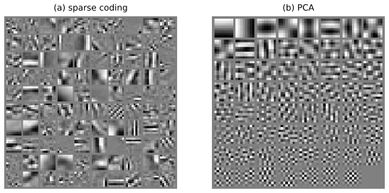
28.6.6 Nonlinear ICA
p. 978 The nonlinear extensions of ICA are similar to variational autoencoders (Chapter 21); without further assumptions the nonlinear problem is not identifiable (any measure-preserving transformation of the sources is again independent), and the identifiable versions use auxiliary variables or temporal structure (Khemakhem et al. 2020).
Practice problems
The book has no end-of-chapter exercises for Chapter 28, so here are three short problems of my own, with complete solutions (hidden).
Practice problem 28.1 (shrinkage by a spike-and-slab prior). A coefficient has the spike-and-slab prior \(0.8\,\delta_0+0.2\,\N(0,1)\) and is observed with noise as \(y=x+\N(0,1)\). (a) Find the posterior probability that \(x\) is non-zero and the posterior mean when \(y=3\). (b) Compare with a Gaussian prior \(\N(0,1)\), and say what a Laplace prior with \(\lambda=1.4\) gives for \(y=12\). (c) Explain why none of the posterior means is exactly zero for \(y\ne0\).
Solution
(a) By gap 28.1(iv) with \(\pi=0.2\), \(\sigma_0=s=1\): \(p_Y(3)=0.2\,\N(3\given0,2)+0.8\,\N(3\given0,1)\). \(\N(3\given0,2)=e^{-9/4}/\sqrt{4\pi}=0.1054/3.545=0.02973\) and \(\N(3\given0,1)=0.004432\), so the slab weight is \(w=\frac{0.2\times0.02973}{0.2\times0.02973+0.8\times0.004432}=\frac{0.005946}{0.009492}=0.626\). The posterior mean is \(w\,y\,\sigma_0^2/(\sigma_0^2+s^2)=0.626\times3\times\frac12=0.940\) (the value computed by the code). (b) The Gaussian prior gives the linear rule \(y\sigma_0^2/(\sigma_0^2+s^2)=1.5\) (no sparsity); the Laplace rule at \(y=12\) is \(12-\lambda s^2=10.6\) to four digits, by gap 28.1(iii), a constant shift of 1.4. (c) By gap 28.1(i), \(\E[x\given y]=y\,\E[\kappa\given y]\) with \(\kappa>0\) for the scale mixtures with continuous scale; for the spike and slab \(\E[x\given y]=w(y)\,y/2\) and \(w(y)>0\) always, because the slab has full support; exact zeros occur in the posterior probability \(1-w(y)\) of the spike or in the posterior mode (the lasso), not in the mean.
Practice problem 28.2 (how many parameters, how much work). For \(D=64\) pixels and \(K=5\) clusters, count the parameters of (a) one factor analyser with \(L=4\) factors, (b) a five-component GMM with full covariances, (c) a five-component MFA with \(L=4\) and a shared diagonal noise. (d) How many arithmetic operations (to leading order) does one log-density evaluation of a component cost in each case?
Solution
(a) \[ D(L+1)-\frac{L(L-1)}2=64\cdot5-6=314 \] identifiable parameters (the mean, \(\bm W\) up to rotation, and \(\bm\Psi\)); a full covariance would have \(D(D+1)/2=2080\) and a diagonal one 64 (confirmed for a small case by the Jacobian rank). (b) \[ K\Big(D+\frac{D(D+1)}2\Big)+K-1=5\,(64+2080)+4=10\,724. \] (c) \[ K\,D(L+1)+D+K-1=5\cdot64\cdot5+64+4=1668, \] or \(1638\) after removing the rotation redundancy \(K\,L(L-1)/2=30\) of the \(\bm W_k\): about \(6.5\) times fewer than the GMM. (d) The full-covariance Gaussian needs a Cholesky solve, \(O(D^2)=4096\) operations per point after an \(O(D^3)\) factorisation shared by all points; the MFA component needs \(\bm W^{\mathrm T}\bm\Psi^{-1}(\bm x-\bm\mu)\) (\(DL=256\)) and a solve with the \(L\times L\) matrix (\(L^2\)), i.e. \(O(LD+L^2)\) per point after \(O(DL^2+L^3)\) once (lemmas of gap 28.4), roughly \(16\) times cheaper.
Practice problem 28.3 (why a non-Gaussian source fixes the angle). Two independent sources have zero mean, unit variance and excess kurtosis \(\kappa\) (uniform: \(-1.2\); Laplace: \(3\); Gaussian: \(0\)). Let \(z_1=\cos\theta\,s_1+\sin\theta\,s_2\). (a) Show that the excess kurtosis of \(z_1\) is \(\kappa(1-\frac12\sin^22\theta)\). (b) For which \(\theta\) is \(|\mathrm{kurt}(z_1)|\) largest, and what does this say about ICA? (c) What happens for Gaussian sources?
Solution
(a) The fourth cumulant \(\kappa_4\) of a sum of independent variables is the sum of the fourth cumulants, and it is homogeneous of degree 4: \(\kappa_4(a s_1+b s_2)=a^4\kappa_4(s_1)+b^4\kappa_4(s_2)\) (the cumulant generating function of a sum of independent variables is additive). With unit variance, \(\kappa_4\) is the excess kurtosis \(\kappa\), so \(\mathrm{kurt}(z_1)=(\cos^4\theta+\sin^4\theta)\kappa\), and \[ \cos^4\theta+\sin^4\theta=1-2\sin^2\theta\cos^2\theta=1-\tfrac12\sin^22\theta. \] (b) The factor equals 1 at \(\theta=0,90^\circ,\dots\) (the true sources) and its minimum \(\frac12\) at \(45^\circ\) (a half-and-half mixture): \(|\mathrm{kurt}|\) is largest at the true angles, \(-1.2\) against \(-0.6\) for uniform sources and \(3\) against \(1.5\) for Laplace sources (simulated with \(2\times10^6\) draws: \(-1.200\), \(-0.900\), \(-0.600\) at \(0,22.5^\circ,45^\circ\); \(3.04\), \(2.27\), \(1.51\)). Mixing makes the sum more Gaussian (the central limit effect), so unmixing means maximising \(|\)non-Gaussianity\(|\), the idea behind projection pursuit and negentropy, and the sign of \(\kappa\) tells whether the true angle is a maximum (super-Gaussian) or minimum of the kurtosis itself, the caveat of gap 28.16. (c) \(\kappa=0\) for every \(\theta\): the contrast is identically zero (and the whole distribution is rotation invariant), so no angle is preferred: the sources are not identifiable.
Demonstrations
- Scale mixtures and their shrinkage rules (Section 28.2.3): Gaussian, Student, Laplace, horseshoe and spike-and-slab priors; the density, the tails, and the rule \(\E[x\given y]\) at any noise level.
- ICA and the rotation angle (Sections 28.6.2–28.6.3): rotate whitened mixtures of uniform, Laplace, mixed or Gaussian sources; the ICA objective, the kurtosis and the scatter plot.
- Collapsed Gibbs sampling for LDA (Supplement S28.1.1): sweeps on the bank, river, money corpus; the assignments, the topic-word estimates and the collapsed log-joint.
Python code for every figure: code index. Data used by the demos: data/ch28-ica.json, data/ch28-lda.json. Companion demos: Volume 1 (PPCA by EM, PCA, SVD, whitening).
Notes on the book
Points where the book is imprecise or wrong
- (28.14). "Laplace\((x\given0,\lambda)\)" must mean the rate \(\lambda\) (scale \(1/\lambda\), as in (28.158)) for the mixing law \(\mathrm{Ga}(\tau^2\given1,\lambda^2/2)\) to give the Laplace density \(\frac\lambda2e^{-\lambda|x|}\); with the scale convention the exponent would be \(1/\lambda\).
- (28.21)–(28.22). The log of a zero-mean Gaussian is \(-\frac12\bm x^{\mathrm T}\bm\Sigma^{-1}\bm x+a_k\); the factor \(\frac12\) is missing in both equations (Section 28.2.4.1).
- (28.102). \(\bm v=\sigma_x^{-2}\bm C\bm W_x\bm w_y\) has non-conforming dimensions (\(\bm C\) is \(L\times L\), \(\bm W_x\) is \(D_x\times L\)); the correct vector is \(\sigma_x^{-2}\bm W_x\bm C\bm w_y\) (gap 28.7).
- Section 28.3.4.3. The equivalence "MLE of the CCA model is CCA" holds when the private subspaces are large enough to carry arbitrary private covariances; with isotropic noise and small private subspaces it does not (gap 28.7).
- Section 28.4.1. "\(\alpha_k=\beta_k=0\) and the MLE of \(\bm W\) recover NMF": the improper prior \(p(z)\propto1/z\) has an unbounded MAP objective; plain maximum likelihood (no prior on the codes), or the flat prior \(\alpha=1,\beta=0\), is NMF with the KL divergence (gap 28.10).
- (28.126). The determinant in the GP-LVM likelihood is \(|\bm K_\sigma|=|\bm K+\sigma^2\bm I|\), not \(|\bm K_z|\) (gap 28.9).
- Section 28.5.2. The Dirichlet covariance is \(\Sigma_{ij}=-\alpha_i\alpha_j/(\alpha_0^2(\alpha_0+1))\), not \(-\alpha_i\alpha_j\); and in (28.133) \(z\) is the draw \(\mathrm{softmax}(\bm\epsilon)\) itself, not a categorical sample of it (gap 28.15).
- (28.143). \(x_{nj}=\sum_iA_{ij}z_{nj}\) has the wrong indices; it is \(x_{nj}=\sum_iA_{ji}z_{ni}\).
- (28.154), (28.157). Negentropy equals the log-likelihood only when the model marginals are the true ones; the exact identity is \(\mathrm{NLL}=\mathbb H(\tilde{\bm x})+\mathrm{TC}+\sum_j\Dkl(q_j\|p_j)\). The entropy formula (28.157) is for the noiseless nonlinear encoder (gap 28.17).
- Section 28.6.2. A super-Gaussian prior "helps identifiability", but maximum likelihood with a super-Gaussian prior puts the true unmixing at a maximum of the objective when the sources are sub-Gaussian (uniform), so the prior must match the sign of the kurtosis (gap 28.16).
- (28.160). Without a norm constraint on the columns of \(\bm W\) the joint problem is degenerate (\(\bm W\to c\bm W\), \(\bm Z\to\bm Z/c\) drives the penalty to 0) (gap 28.19).
- Supplement S(28.8). The second factor's denominator \(L_i+K\alpha\) is the same for every \(k\) and cancels (it is \(L_i-1+K\alpha\) if the token is removed first); and S(28.13), (S28.20) differ by whether the Dirichlet pseudo-count is \(\beta\) or \(\beta-1\) in the EM (MAP) and VB versions (gaps 28.12, 28.13).
References
- Murphy, K. P. (2023). Probabilistic Machine Learning: Advanced Topics. MIT Press, Cambridge, MA. Chapter 28, pp. 929–978, and supplementary material, Chapter 28. probml.github.io/pml-book/book2.html.
- Arora, S., Ge, R., Halpern, Y., Mimno, D., Moitra, A., Sontag, D., Wu, Y. and Zhu, M. (2013). A practical algorithm for topic modeling with provable guarantees. International Conference on Machine Learning.
- Bach, F. R. and Jordan, M. I. (2005). A probabilistic interpretation of canonical correlation analysis. Technical Report 688, Department of Statistics, University of California, Berkeley.
- Beal, M. J. (2003). Variational Algorithms for Approximate Bayesian Inference. PhD thesis, University College London.
- Bell, A. J. and Sejnowski, T. J. (1995). An information-maximization approach to blind separation and blind deconvolution. Neural Computation, 7(6), 1129–1159.
- Bhattacharya, A. and Dunson, D. B. (2011). Simplex factor models for multivariate unordered categorical data. Journal of the American Statistical Association, 107(497), 362–377.
- Bishop, C. M. (1999). Bayesian PCA. Advances in Neural Information Processing Systems, 11.
- Blei, D. M. and Lafferty, J. D. (2006). Dynamic topic models. International Conference on Machine Learning. Blei, D. M. and Lafferty, J. D. (2007). A correlated topic model of Science. Annals of Applied Statistics, 1(1), 17–35.
- Blei, D. M., Ng, A. Y. and Jordan, M. I. (2003). Latent Dirichlet allocation. Journal of Machine Learning Research, 3, 993–1022.
- Bouchard, G. and Triggs, B. (2004). The trade-off between generative and discriminative classifiers. COMPSTAT.
- Buntine, W. and Jakulin, A. (2006). Discrete component analysis. Subspace, Latent Structure and Feature Selection, Lecture Notes in Computer Science 3940, 1–33.
- Canny, J. (2004). GaP: a factor model for discrete data. ACM SIGIR.
- Carvalho, C. M., Polson, N. G. and Scott, J. G. (2010). The horseshoe estimator for sparse signals. Biometrika, 97(2), 465–480.
- Collins, M., Dasgupta, S. and Schapire, R. E. (2002). A generalization of principal components analysis to the exponential family. Advances in Neural Information Processing Systems, 14.
- Comon, P. (1994). Independent component analysis, a new concept? Signal Processing, 36(3), 287–314.
- Darmois, G. (1953). Analyse générale des liaisons stochastiques. Revue de l'Institut International de Statistique, 21, 2–8. Skitovich, V. P. (1953). On a property of the normal distribution. Doklady Akademii Nauk SSSR, 89, 217–219.
- Dieng, A. B., Ruiz, F. J. R. and Blei, D. M. (2019). The dynamic embedded topic model. arXiv:1907.05545.
- Gaussier, E. and Goutte, C. (2005). Relation between PLSA and NMF and implications. ACM SIGIR.
- Ghahramani, Z. and Beal, M. J. (2000). Variational inference for Bayesian mixtures of factor analysers. Advances in Neural Information Processing Systems, 12. Ghahramani, Z. and Hinton, G. E. (1996). The EM algorithm for mixtures of factor analyzers. Technical Report CRG-TR-96-1, University of Toronto.
- Griffiths, T. L. and Steyvers, M. (2004). Finding scientific topics. Proceedings of the National Academy of Sciences, 101, 5228–5235.
- Guo, Y. and Schuurmans, D. (2008). Efficient global optimization for exponential family PCA and low-rank matrix factorization. Allerton Conference on Communication, Control, and Computing.
- Griffiths, T. L., Steyvers, M., Blei, D. M. and Tenenbaum, J. B. (2004). Integrating topics and syntax. Advances in Neural Information Processing Systems, 17.
- Hoffman, M. D., Blei, D. M. and Bach, F. (2010). Online learning for latent Dirichlet allocation. Advances in Neural Information Processing Systems, 23. Hoffman, M. D., Blei, D. M., Wang, C. and Paisley, J. (2013). Stochastic variational inference. Journal of Machine Learning Research, 14, 1303–1347.
- Hofmann, T. (1999). Probabilistic latent semantic analysis. Uncertainty in Artificial Intelligence.
- Hyvärinen, A. and Oja, E. (2000). Independent component analysis: algorithms and applications. Neural Networks, 13(4–5), 411–430.
- Jaakkola, T. S. and Jordan, M. I. (2000). Bayesian parameter estimation via variational methods. Statistics and Computing, 10, 25–37.
- Khemakhem, I., Kingma, D. P., Monti, R. P. and Hyvärinen, A. (2020). Variational autoencoders and nonlinear ICA: a unifying framework. AISTATS.
- Lawrence, N. D. (2005). Probabilistic non-linear principal component analysis with Gaussian process latent variable models. Journal of Machine Learning Research, 6, 1783–1816.
- Lee, D. D. and Seung, H. S. (1999). Learning the parts of objects by non-negative matrix factorization. Nature, 401, 788–791. Lee, D. D. and Seung, H. S. (2001). Algorithms for non-negative matrix factorization. Advances in Neural Information Processing Systems, 13.
- Lopes, H. F. and West, M. (2004). Bayesian model assessment in factor analysis. Statistica Sinica, 14, 41–67.
- MacKay, D. J. C. (2003). Information Theory, Inference, and Learning Algorithms. Cambridge University Press.
- Mairal, J., Bach, F., Ponce, J. and Sapiro, G. (2010). Online learning for matrix factorization and sparse coding. Journal of Machine Learning Research, 11, 19–60.
- Olshausen, B. A. and Field, D. J. (1996). Emergence of simple-cell receptive field properties by learning a sparse code for natural images. Nature, 381, 607–609.
- Paatero, P. and Tapper, U. (1994). Positive matrix factorization. Environmetrics, 5(2), 111–126.
- Pritchard, J. K., Stephens, M. and Donnelly, P. (2000). Inference of population structure using multilocus genotype data. Genetics, 155, 945–959.
- Richardson, E. and Weiss, Y. (2018). On GANs and GMMs. Advances in Neural Information Processing Systems, 31.
- Roweis, S. (1997). EM algorithms for PCA and SPCA. Advances in Neural Information Processing Systems, 10.
- Stephens, M. (2000). Dealing with label switching in mixture models. Journal of the Royal Statistical Society B, 62(4), 795–809.
- Tipping, M. E. (1998). Probabilistic visualisation of high-dimensional binary data. Advances in Neural Information Processing Systems, 11. Tipping, M. E. and Bishop, C. M. (1999). Probabilistic principal component analysis. Journal of the Royal Statistical Society B, 61(3), 611–622.
- Udell, M., Horn, C., Zadeh, R. and Boyd, S. (2016). Generalized low rank models. Foundations and Trends in Machine Learning, 9(1), 1–118.
- Welling, M., Chemudugunta, C. and Sutherland, N. (2008). Deterministic latent variable models and their pitfalls. SIAM International Conference on Data Mining.
- Yu, S., Yu, K., Tresp, V., Kriegel, H.-P. and Wu, M. (2006). Supervised probabilistic principal component analysis. ACM SIGKDD.
- Zoran, D. and Weiss, Y. (2011). From learning models of natural image patches to whole image restoration. International Conference on Computer Vision.
- Ahn, J.-H. and Oh, J.-H. (2003). A constrained EM algorithm for principal component analysis. Neural Computation, 15(1), 57–65.
- Dieng, A. B., Wang, C., Gao, J. and Paisley, J. (2017). TopicRNN: a recurrent neural network with long-range semantic dependency. International Conference on Learning Representations.
- Erosheva, E., Fienberg, S. and Lafferty, J. (2004). Mixed-membership models of scientific publications. Proceedings of the National Academy of Sciences, 101, 5220–5227.
- Friedman, J. H. and Tukey, J. W. (1974). A projection pursuit algorithm for exploratory data analysis. IEEE Transactions on Computers, C-23(9), 881–890.
- Hoffman, M. D. (2017). Learning deep latent Gaussian models with Markov chain Monte Carlo. International Conference on Machine Learning.
- Hotelling, H. (1936). Relations between two sets of variates. Biometrika, 28, 321–377.
- Kaiser, H. F. (1958). The varimax criterion for analytic rotation in factor analysis. Psychometrika, 23, 187–200.
- Kavukcuoglu, K., Ranzato, M. and LeCun, Y. (2008). Fast inference in sparse coding algorithms with applications to object recognition. arXiv:1010.3467.
- Khan, M. E., Bouchard, G., Murphy, K. P. and Marlin, B. M. (2010). Variational bounds for mixed-data factor analysis. Advances in Neural Information Processing Systems, 23.
- Linsker, R. (1988). Self-organization in a perceptual network. Computer, 21(3), 105–117.
- Marlin, B. (2003). Modeling user rating profiles for collaborative filtering. Advances in Neural Information Processing Systems, 16.
- Miao, Y., Yu, L. and Blunsom, P. (2016). Neural variational inference for text processing. International Conference on Machine Learning. Srivastava, A. and Sutton, C. (2017). Autoencoding variational inference for topic models. International Conference on Learning Representations.
- Paisley, J. and Carin, L. (2009). Nonparametric factor analysis with beta process priors. International Conference on Machine Learning.
- Teh, Y. W., Jordan, M. I., Beal, M. J. and Blei, D. M. (2006). Hierarchical Dirichlet processes. Journal of the American Statistical Association, 101(476), 1566–1581.
- Wallach, H. M., Murray, I., Salakhutdinov, R. and Mimno, D. (2009). Evaluation methods for topic models. International Conference on Machine Learning.
- West, M. (2003). Bayesian factor regression models in the "large p, small n" paradigm. Bayesian Statistics, 7, 733–742.
- Zong, B., Song, Q., Min, M. R., Cheng, W., Lumezanu, C., Cho, D. and Chen, H. (2018). Deep autoencoding Gaussian mixture model for unsupervised anomaly detection. International Conference on Learning Representations.
The numerical statements in the text (the scale-mixture identities and shrinkage rules; the mixture, determinant and inversion lemmas, log-sum-exp and label-switching facts; the factor-analysis likelihood, posterior, rotation invariance and parameter count; the mixture of factor analysers, its imputation and its monotone EM; the supervised-PCA predictive, the reduced-rank regression and the canonical correlations; the binary-PCA bound; the GP-LVM optimum and its gradient; the NMF updates and their Poisson interpretation; the Dirichlet moments, the collapsed marginal and Gibbs conditional, the mean-field ELBO and the batch and online variational algorithms; the ICA identity, the FastICA fixed point and the unmixing errors; the lasso solution and the scale degeneracy; the Fourier eigenvectors of a circulant covariance; and the denoising gain) were confirmed numerically.