Statistics
Statistics is the inverse of probability: given data, infer the parameters that produced them. This chapter sets the Bayesian and the frequentist answers side by side, then builds the Bayesian toolbox that the rest of the book uses: conjugate families (up to the normal inverse Wishart), default and invariant priors, hierarchical models and empirical Bayes, model selection by the marginal likelihood and its cross-validation and information-criterion relatives, checks of a fitted model, and the dictionary that turns classical tests into linear models. The supplement adds the number game, informative priors for everyday prediction, and Tweedie's formula.
Ch. 1 Introduction Ch. 2 Probability Ch. 3 Statistics Ch. 4 Graphical models Ch. 5 Information theory Ch. 6 Optimisation Ch. 7 Inference algorithms Ch. 8 Gaussian filtering Ch. 9 Message passing Ch. 10 Variational inference Ch. 11 Monte Carlo Ch. 12 MCMC Ch. 13 Sequential Monte Carlo Ch. 14 Predictive models Ch. 15 GLMs Ch. 16 Deep networks Ch. 17 Bayesian neural networks Ch. 18 Gaussian processes Ch. 19 Beyond iid Ch. 20 Generative models Ch. 21 VAEs Ch. 22 Autoregressive models Ch. 23 Normalizing flows Ch. 24 Energy-based models Ch. 25 Diffusion models Ch. 26 GANs Ch. 27 Discovery methods Ch. 28 Latent factor models Ch. 29 State-space models Ch. 30 Graph learning Ch. 31 Nonparametric Bayes Ch. 32 Representation learning Ch. 33 Interpretability Ch. 34 Decision making Ch. 35 Reinforcement learning Ch. 36 Causality
How to read these notes
They follow the book. Sections carry the book's numbers (3.2, 3.4.3, ...) and displayed equations that appear in the book carry its equation numbers, e.g. \((3.38)\). Sections of the online supplement are labelled (supplement) and numbered S3.1, S3.2, S3.3, placed where they belong in the chapter. Equations without a number are steps the book skips.
Filling the gaps. Wherever the book says "one can show", leaves a proof out or quotes a result, an orange Filling the gap box gives a complete argument. Proofs start hidden: open one with its bar, or use the button below. Results already proved in the first volume of the course or in All of Statistics are stated and linked, not repeated.
Figures and demonstrations. Every figure that is computed is reproduced from scratch by the Python code; five diagrams are not (listed in the code). Where the book's data are not freely available a seeded simulation with the stated parameters replaces them, and the caption says so.
Main reference
K. P. Murphy, Probabilistic Machine Learning: Advanced Topics, MIT Press (2023; the December 2025 draft and its online supplement are used), Chapter 3, pages 63–142, and Supplement Chapter 3, pages 23–37 (book website: probml.github.io/pml-book/book2.html). Section, equation, figure and exercise numbers refer to this book. The chapter has no end-of-chapter exercises; three practice problems are given instead.
The explanations, derivations, figures and code are my own; equations are cited by their numbers in the book.
Companion courses
Chapter 3 is the second pass over material met in the first volume. Overlapping material, with proofs, is here:
- Probabilistic Machine Learning: An Introduction, Chapter 4: the beta-binomial model (gap 4.7, 4.8, 4.9), mixtures of conjugate priors (4.10), Dirichlet-multinomial (4.11), the Gaussian posterior (4.12), HPD (4.14), the bootstrap (4.16), Berger's two-integer example (4.18), empirical Bayes (4.13), and Fisher information with asymptotic normality (Result 4.4).
- All of Statistics: 9.7 asymptotic normality, 8.3 bootstrap intervals, 11.6 flat and noninformative priors, 10.2 p-values.
- Bayesian and Probabilistic Machine Learning (Bishop): 2.3.6 Bayesian inference for the Gaussian, 2.4.3 noninformative priors.
What this chapter adds: the normal inverse chi-squared and normal inverse Wishart families with their marginals and predictives, Jeffreys, invariant and reference priors, hierarchical models with exact computation, the marginal likelihood against LOO, BIC, AIC and WAIC, posterior predictive checks, tests as linear models, ignorability of missing data, and Tweedie's formula.
The chapter at a glance
- 3.2 The Bayesian recipe on the coin: posterior, MAP, mean, credible and HPD intervals, plug-in against posterior predictive, exchangeability (gap 3.4).
- 3.3 The frequentist recipe: sampling distributions, the bootstrap against the posterior (gap 3.5), Fisher information (gap 3.6, 3.7), and why p-values and confidence intervals mislead (gap 3.8).
- 3.4 Conjugate families: Dirichlet, normal inverse chi-squared (gap 3.9), normal inverse Wishart (gap 3.10), the exponential family (gap 3.11), robust and variance priors.
- 3.5 Default priors: maximum entropy, Jeffreys (gap 3.16), invariant and reference priors.
- 3.6–3.7 Hierarchical models and empirical Bayes: rat tumours (gap 3.18) and eight schools (gap 3.19), the funnel (gap 3.20), n-gram smoothing (gap 3.22).
- 3.8–3.9 Model selection and checking: evidence, BMA, LOO, BIC, AIC, WAIC (gaps 3.27–3.29), posterior predictive checks.
- 3.10–3.11 Tests as linear models, and missing data.
- S3.1–S3.3 The number game, informative priors, Tweedie's formula.
Notation. Data \(\mathcal D\), parameters \(\theta\), likelihood \(p(\mathcal D\given\theta)\), prior \(p(\theta)\). A breve (written \(\breve a\)) marks the prior hyperparameter and a hat (\(\hat a\)) the posterior one, as in the book: the posterior of \(\theta\) in the beta model is \(\Beta(\hat a,\hat b)\) with \(\hat a=\breve a+N_1\). I write \(\breve{}\) quantities as \(a_0\) when a single subscript is clearer.
3.1 Introduction
p. 63 Probability computes \(p(\mathcal D\given\theta)\) for known parameters; statistics inverts the problem and wants \(p(\theta\given\mathcal D)\) (Bayesian) or the behaviour of estimators over repeated datasets (frequentist). The two views are compared as decision procedures in Chapter 34 of the book.
3.2 Bayesian statistics
p. 63 Treat \(\theta\) as unknown and \(\mathcal D\) as fixed, and update by Bayes' rule \[ p(\theta\given\mathcal D)=\frac{p(\theta)\,p(\mathcal D\given\theta)}{p(\mathcal D)},\qquad p(\mathcal D)=\int p(\theta')\,p(\mathcal D\given\theta')\,\d\theta'. \tag{3.1} \] The factors are the prior, the likelihood, the posterior and the marginal likelihood (evidence).
3.2.1 Tossing coins
3.2.1.1–3.2.1.3 Likelihood, prior and posterior
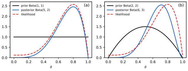
pp. 64–65 For iid tosses \(y_n\in\{0,1\}\) with heads probability \(\theta\), the likelihood is \[p(\mathcal D\given\theta)=\theta^{N_1}(1-\theta)^{N_0}\] (3.2); the counts \((N_1,N_0)\) are sufficient. A binomial observation of \(y\) heads in \(N\) tosses has likelihood \(\binom Ny\theta^y(1-\theta)^{N-y}\) (3.3), proportional to the Bernoulli one in \(\theta\), so inference about \(\theta\) is identical. With prior \[\Beta(\theta\given\breve\alpha,\breve\beta)\propto\theta^{\breve\alpha-1}(1-\theta)^{\breve\beta-1}\] (3.5) the posterior is \[ p(\theta\given\mathcal D)\propto\theta^{N_1+\breve\alpha-1}(1-\theta)^{N_0+\breve\beta-1}=\Beta(\theta\given\hat\alpha,\hat\beta),\quad\hat\alpha=\breve\alpha+N_1,\ \hat\beta=\breve\beta+N_0. \tag{3.6} \] The hyperparameters act as pseudocounts, and \(\breve N=\breve\alpha+\breve\beta\) is the equivalent sample size of the prior.
3.2.1.4–3.2.1.6 MAP, mean and variance
pp. 65–67 The posterior mode is \[\hat\theta_{\rm map}=(\breve\alpha+N_1-1)/(\breve\alpha+\breve\beta+N-2)\] (3.8), the MLE \(N_1/N\) under a uniform prior (3.9), and the add-one estimate \((N_1+1)/(N+2)\) under Beta(2,2) (3.10). The posterior mean \(\hat\alpha/\hat N\) (3.11) is a convex combination of the prior mean \(m=\breve\alpha/\breve N\) and the MLE with weight \(\lambda=\breve N/\hat N\) on the prior (3.12)–(3.13). The posterior variance is \[ \var[\theta\given\mathcal D]=\frac{\hat\alpha\hat\beta}{(\hat\alpha+\hat\beta)^2(\hat\alpha+\hat\beta+1)}\;\approx\;\frac{\hat\theta(1-\hat\theta)}{N}\quad(N\gg\breve N), \tag{3.15--3.17} \] so the standard error falls as \(1/\sqrt N\) and is largest at \(\hat\theta=\tfrac12\). The proofs (beta moments, mode, convex combination) are in Filling the gap 4.7 of the first volume.
Filling the gap 3.1: why Bernoulli and binomial data give the same posterior, and the origin of the \(\hat\theta(1-\hat\theta)/N\) variance pp. 64, 67
Derivation
Same posterior. Bayes' rule multiplies the prior by the likelihood and normalises over \(\theta\). Any factor of the likelihood that does not depend on \(\theta\), such as \(\binom Ny\), cancels in the normalisation. The Bernoulli sequence with \(N_1\) ones has probability \(\theta^{N_1}(1-\theta)^{N_0}\); the binomial count has probability \(\binom N{N_1}\) times this. The posteriors therefore coincide.
Large-sample variance. Put \(\hat\alpha=\breve\alpha+N_1\), \(\hat\beta=\breve\beta+N_0\), \(\hat N=\hat\alpha+\hat\beta=N+\breve N\). Then \(\var=m_p(1-m_p)/(\hat N+1)\) with \(m_p=\hat\alpha/\hat N\) the posterior mean. When \(N\gg\breve N\): \[m_p=\frac{N_1+\breve\alpha}{N+\breve N}\to N_1/N=\hat\theta\] and \(\hat N+1\sim N\), giving (3.16). The ratio of the exact variance to \(\hat\theta(1-\hat\theta)/N\) is \(1+O(1/N)\), so the credible interval \[\hat\theta\pm2\sqrt{\hat\theta(1-\hat\theta)/N}\] is the same as the Wald interval of frequentist statistics to first order.
Maximal at \(\hat\theta=\frac12\). \(\hat\theta(1-\hat\theta)\) is a concave parabola with maximum \(1/4\) at \(\frac12\) and tends to 0 at 0 and 1: a coin that always shows heads is easier to identify than a fair one. \(\square\)
3.2.1.7 Credible intervals
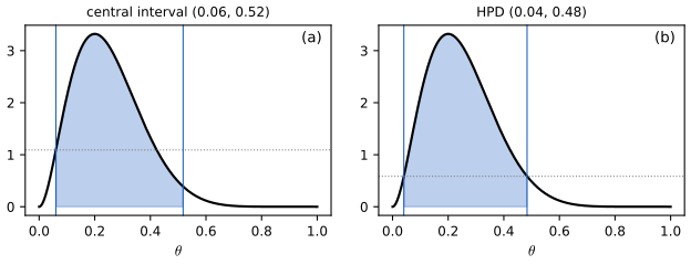
pp. 67–68 A \(100(1-\alpha)\%\) credible interval \((\ell,u)\) satisfies \[P(\ell\le\theta\le u\given\mathcal D)=1-\alpha\] (3.18). The central interval puts \(\alpha/2\) in each tail, \(\ell=F^{-1}(\alpha/2)\), \(u=F^{-1}(1-\alpha/2)\); the highest posterior density (HPD) region is \(\{\theta:p(\theta\given\mathcal D)\ge p^*\}\) with \(p^*\) chosen so that the mass is \(1-\alpha\) (3.19)–(3.20). For Beta(3,9) the central interval is \((0.06,0.52)\) and the HPD interval \((0.04,0.48)\). The HPD interval is the shortest interval of the given mass and has equal density at its two ends: see Filling the gap 4.14.
3.2.1.8–3.2.1.9 Posterior predictive and marginal likelihood
pp. 68–70 The posterior predictive \[p(y\given\mathcal D)=\int p(y\given\theta)p(\theta\given\mathcal D)\,\d\theta\] (3.21) averages the model over the posterior; the plug-in approximation \(p(y\given\hat\theta)\) (3.22) replaces the posterior by a point mass (3.23)–(3.24) and overfits: after three heads in a row the MLE says tails are impossible. For the beta model the predictive is the posterior mean, \[p(y=1\given\mathcal D)=\hat\alpha/(\hat\alpha+\hat\beta)\] (3.26), which under a uniform prior is Laplace's rule of succession \((N_1+1)/(N+2)\) (3.27). The marginal likelihood is the ratio of normalisers \[p(\mathcal D)=B(\hat\alpha,\hat\beta)/B(\breve\alpha,\breve\beta)\] (3.30); under the Jeffreys prior \(\Beta(\frac12,\frac12)\) this is the Krichevski–Trofimov estimator \(\frac1\pi B(N_1+\frac12,N_0+\frac12)\) (3.31) since \(B(\frac12,\frac12)=\pi\). See gaps 4.8 and 4.9 of the first volume.
See also (demonstration in the first volume): the beta-binomial model.
S3.1 Bayesian concept learning (supplement)
Supplement pp. 23–32 The book points here (Section 3.2.1) for a gentler introduction to Bayes. A child learns "dog" from positive examples only; the learner has a hypothesis space \(\mathcal H\) of concepts \(h\), and computes \(p(h\given\mathcal D)\). Version spaces (keep every hypothesis consistent with the data) cannot explain why after \(\{16,8,2,64\}\) people infer "powers of two" rather than "even numbers" or "powers of two except 32": all are consistent. Bayes' rule with a size-sensitive likelihood and a prior over concepts does.
S3.1.1 Learning a discrete concept: the number game
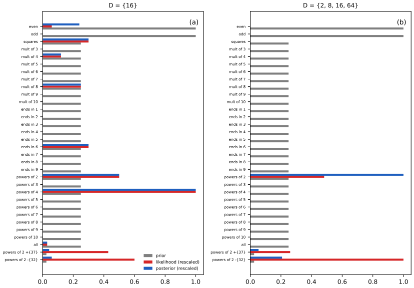
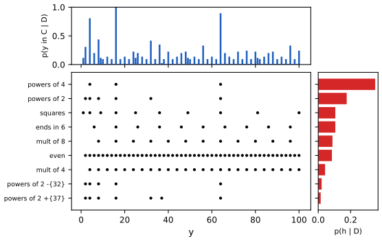
Supplement pp. 23–29 Numbers lie in \(1..100\); a concept is a subset (even numbers, powers of two, "numbers ending in 9", intervals). Likelihood. Under strong sampling the examples are drawn uniformly with replacement from the extension of \(h\): \[ p(\mathcal D\given h)=\prod_{n=1}^N\frac{\mathbb 1[y_n\in h]}{\mathrm{size}(h)}=\Big(\frac1{\mathrm{size}(h)}\Big)^N\mathbb 1[\mathcal D\subseteq h] \tag{S3.1} \] the size principle, which favours the smallest consistent hypothesis (Occam's razor). For \(D=\{16\}\), \(p(D\given h_{\rm two})=\frac16\) (six powers of two below 100) and \(p(D\given h_{\rm even})=\frac1{50}\); after \(\{16,8,2,64\}\) the likelihood ratio is \((50/6)^4=4823\) ("almost 5000:1"). Prior. 30 simple rules (even, odd, squares, multiples of 3 to 10, endings 1 to 9, powers of 2 to 10, all numbers), with even and odd more likely a priori, and two "unnatural" concepts (powers of two plus 37, powers of two except 32) with low prior weight; plus all intervals \([n,m]\). The mixture is \[ p(h)=\pi\,\mathrm{Unif}(h\given\text{rules})+(1-\pi)\,\mathrm{Unif}(h\given\text{intervals}) \tag{S3.2} \] The notes use prior weights 4 (even, odd), 0.1 (unnatural) and 1 (the other rules), normalised (so even and odd get 0.11, unnatural concepts 0.0028 each) and \(\pi=\frac12\) for the full space; the book does not give its numbers. Posterior and predictive. \[p(h\given\mathcal D)\propto p(\mathcal D\given h)p(h)\], and the predictive is the Bayes model average \[p(y\in C\given\mathcal D)=\sum_h\mathbb 1[y\in h]\,p(h\given\mathcal D)\] (S3.3).
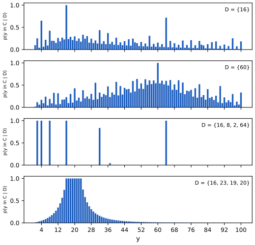
Filling the gap 3.36: the size principle, its exponential strength, and MAP, MLE and plug-in in the number game Supplement pp. 25–29, (S3.1)–(S3.8)
Derivation
Strong against weak sampling. Suppose the teacher picks examples independently and uniformly from the extension of the concept. Then \(p(y\given h)=1/|h|\) for \(y\in h\) and 0 otherwise, and the likelihood of a set of independent examples is (S3.1). If the examples were instead generated independently of \(h\) and merely checked for membership (weak sampling, \(p(y\given h)\propto\mathbb 1[y\in h]\) with a constant independent of \(h\)), all consistent hypotheses would have equal likelihood and size would not matter.
Strength. Let \(h_1\subset h_2\) both contain \(\mathcal D\). The posterior odds are \[\frac{p(h_1\given\mathcal D)}{p(h_2\given\mathcal D)}=\big(\frac{|h_2|}{|h_1|}\big)^N\frac{p(h_1)}{p(h_2)}\]: the data multiply the prior odds by the size ratio to the power \(N\), i.e. exponentially in the number of examples, which is the "suspicious coincidence" argument made exact. With \(N=4\), \(|h_2|/|h_1|=50/6\) gives a factor 4823, which is why even numbers lose to powers of two despite even's larger prior (4 against 1). The same mechanism with \(|h_2|/|h_1|=6/5\) (the unnatural concept against powers of 2) gives only 2.07, far below the prior ratio 10, so the unnatural concept stays at 0.16 against 0.79: a low prior prevents overfitting to the missing 32.
MAP, MLE, plug-in. With \[\hat h_{\rm map}=\argmax_h\{\log p(\mathcal D\given h)+\log p(h)\}\] (S3.5), the log likelihood \(-N\log|h|\) grows linearly with \(N\) while \(\log p(h)\) is fixed, so the prior is eventually overwhelmed and MAP tends to the MLE (S3.6), the smallest consistent hypothesis. The plug-in predictive \[p(y\given\hat h)=\mathbb 1[y\in\hat h]/|\hat h|\] (S3.8) is a point mass on the posterior. For \(D=\{16\}\) the smallest consistent rule is "powers of 4" (size 3), so the plug-in predicts only \(\{4,16,64\}\): overconfident, whereas the posterior average is diffuse (Figure S3.4). Correction to the book: it says that after \(\{16,8,2,64\}\) "the MLE broadens to powers of two". In the space that contains the unnatural concept "powers of 2 except 32" the maximum likelihood hypothesis is that concept (size 5 against 6), and only the MAP, which includes the prior, selects "powers of 2"; the statement holds if the unnatural concepts are removed. All of these were confirmed numerically. \(\square\)
S3.1.2 Learning a continuous concept: the healthy levels game
Supplement pp. 29–32 Two measurements (cholesterol, insulin) of healthy people; the concept is an axis-parallel rectangle \(h=(\ell_1,\ell_2,s_1,s_2)\) (corner and side lengths) and points are sampled uniformly from it. In one dimension the likelihood is \(s^{-N}\) if \(\ell\le\min\mathcal D\) and \(\max\mathcal D\le\ell+s\), else 0 (S3.9); in 2-d it factorises over the two coordinates (S3.10). With the scale-invariant prior \(p(h)\propto\frac1{s_1}\frac1{s_2}\) (Section 3.5.3) the posterior is \[\propto p(\mathcal D_1\given\ell_1,s_1)p(\mathcal D_2\given\ell_2,s_2)/(s_1s_2)\] (S3.11). With \(y_j^{\min},y_j^{\max}\) the extremes and \(r_j=y_j^{\max}-y_j^{\min}\), the posterior predictive probability that a new point \(\bm y\) lies in the concept is \[ p(\bm y\given\mathcal D)=\Big(\frac1{(1+d(y_1)/r_1)(1+d(y_2)/r_2)}\Big)^{N-1},\qquad d(y_j)=\text{distance of }y_j\text{ to }[y_j^{\min},y_j^{\max}] \tag{S3.12} \] equal to 1 inside the data range and decaying outside; for \(N=1\) the rectangle cannot be inferred. The MLE (smallest enclosing rectangle) predicts a sharp indicator: Bayesian predictions go from broad to narrow as \(N\) grows, plug-in predictions from narrow to broad, and they agree in the limit.
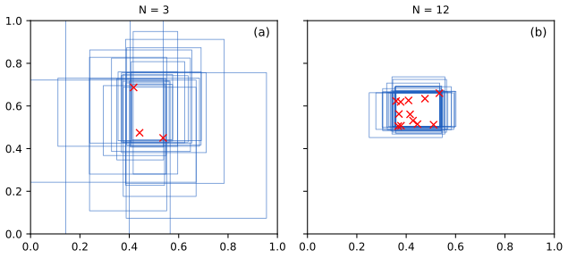
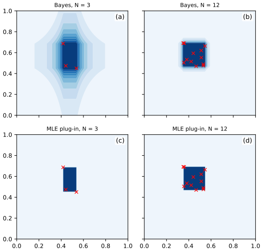
Filling the gap 3.37: the healthy-levels posterior, its exact sampler and the predictive (S3.12) Supplement pp. 30–32, "one can show"
Derivation
One dimension. Posterior \[p(\ell,s\given\mathcal D)\propto s^{-N}\cdot s^{-1}=s^{-N-1}\] on \(\{\ell\le y^{\min},\ \ell+s\ge y^{\max}\}\). Put \(a=y^{\min}-\ell\ge0\), \(b=\ell+s-y^{\max}\ge0\); then \(s=r+a+b\), the map \((\ell,s)\mapsto(a,b)\) has unit Jacobian, and \(p(a,b\given\mathcal D)\propto(r+a+b)^{-(N+1)}\). Its normaliser is \[\int_0^\infty\!\!\int_0^\infty(r+a+b)^{-N-1}\d a\,\d b=\frac{r^{-(N-1)}}{N(N-1)}\] (\(N\ge2\); two successive integrals of a power), so the posterior is proper iff \(N\ge2\).
Predictive. A new point \(y\) lies in the concept iff \(\ell\le y\le\ell+s\). If \(y\in[y^{\min},y^{\max}]\) this holds on the whole support: probability 1. If \(y>y^{\max}\) at distance \(d=y-y^{\max}\), the condition is \(b\ge d\); the integral over \(b\ge d\) is the normaliser with \(r\) replaced by \(r+d\), so the probability is \[\big(\frac{r}{r+d}\big)^{N-1}=(1+d/r)^{-(N-1)}\]; \(y<y^{\min}\) is symmetric. In two dimensions the factors for the two coordinates are independent, giving (S3.12). The predictive is a membership probability, not a density (it equals 1 on the data range).
Exact sampling. With \(t=a+b\), the density of \(t\) is \(\propto t(r+t)^{-N-1}\), with survival function \[S(t)=N(N-1)r^{N-1}\big[\frac{(r+t)^{-(N-1)}}{N-1}-\frac{r(r+t)^{-N}}{N}\big]\] (integrate \((u-r)u^{-N-1}\) with \(u=r+t\)); invert it numerically for \(t\) and draw \(a\sim\mathrm{Unif}(0,t)\) (given \(t\), \((a,b)\) is uniform on the segment \(a+b=t\)); then \(\ell=y^{\min}-a\), \(s=r+t\). The samples of Figure S3.5 and a brute-force grid posterior agree with (S3.12) (grid 0.540 against 0.563 formula at a point just outside the range, the grid being truncated at \(s\le8\) in the heavy tail; Monte Carlo from the exact sampler agrees with the formula to 0.004). The tail of \(s\) is heavy (\(P(t>T)\sim T^{-(N-1)}\)), so for \(N=3\) the sampled rectangles are sometimes very large (Figure S3.5a). \(\square\)
3.2.2 Modeling more complex data
pp. 70–71 For conditional models \(p(y\given\bm x,\theta)\) the quantity of interest is \[p(y\given\bm x,\mathcal D)=\int p(y\given\bm x,\theta)p(\theta\given\mathcal D)\,\d\theta\] (3.32). Integrating out \(\theta\) hedges over infinitely many models and widens the predictive away from the data; the plug-in version (3.33) gives a constant error bar \(\hat\sigma\) (aleatoric uncertainty only) while the Bayesian predictive adds epistemic uncertainty.
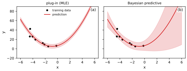
Filling the gap 3.2: the Bayesian predictive of linear regression is a Student t pp. 70–71, Section 15.2
Derivation
Model \(y_n=\bm\phi_n^\T\bm w+\varepsilon_n\), \(\varepsilon_n\sim\mathcal N(0,\sigma^2)\), design matrix \(\bm\Phi\in\R^{N\times D}\) of full column rank, reference prior \(p(\bm w,\sigma^2)\propto\sigma^{-2}\). With \[\hat{\bm w}=(\bm\Phi^\T\bm\Phi)^{-1}\bm\Phi^\T\bm y\] and \(\mathrm{RSS}=\|\bm y-\bm\Phi\hat{\bm w}\|^2\), Pythagoras gives \[\|\bm y-\bm\Phi\bm w\|^2=\mathrm{RSS}+(\bm w-\hat{\bm w})^\T\bm\Phi^\T\bm\Phi(\bm w-\hat{\bm w})\]. The joint posterior is \[ p(\bm w,\sigma^2\given\mathcal D)\propto(\sigma^2)^{-N/2-1}\exp\Big(-\frac{\mathrm{RSS}+(\bm w-\hat{\bm w})^\T\bm\Phi^\T\bm\Phi(\bm w-\hat{\bm w})}{2\sigma^2}\Big). \] So \[\bm w\given\sigma^2\sim\mathcal N(\hat{\bm w},\sigma^2G)\], \(G=(\bm\Phi^\T\bm\Phi)^{-1}\), and, integrating \(\bm w\) (a Gaussian integral giving \((\sigma^2)^{D/2}\)), \[\sigma^2\given\mathcal D\sim\mathrm{IG}\big(\tfrac{N-D}2,\tfrac{\mathrm{RSS}}2\big)\]. For a new input \(\bm\phi_*\), conditionally on \(\sigma^2\), \(y_*=\bm\phi_*^\T\bm w+\varepsilon_*\) is Gaussian with mean \(\bm\phi_*^\T\hat{\bm w}\) and variance \(\sigma^2(1+\bm\phi_*^\T G\bm\phi_*)\). A Gaussian whose variance is \(\sigma^2c\) with \(\sigma^2\sim\mathrm{IG}(\nu/2,\nu s^2/2)\) is a Student t with \(\nu=N-D\) degrees of freedom, location \(\bm\phi_*^\T\hat{\bm w}\) and squared scale \(s^2(1+\bm\phi_*^\T G\bm\phi_*)\), \(s^2=\mathrm{RSS}/(N-D)\) (the scale mixture identity proved in gap 3.9). The standard deviation of the predictive is the scale times \(\sqrt{\nu/(\nu-2)}\), which exists for \(\nu>2\); the second term \(\bm\phi_*^\T G\bm\phi_*\) grows quadratically away from the data, which is the widening in Figure 3.3b. The plug-in predictive keeps only \(\hat\sigma^2_{\rm mle}=\mathrm{RSS}/N\) and so has a constant standard deviation. \(\square\)
Filling the gap 3.3: epistemic uncertainty is a mutual information (footnote 2) p. 71
Derivation
For fixed inputs, define epistemic uncertainty as \(I(\theta;y)=H(y)-H(y\given\theta)\), total minus aleatoric uncertainty, where entropies are taken under the posterior predictive and \[H(y\given\theta)=\E_{p(\theta\given\mathcal D)}H(y\given\theta)\]. It is nonnegative because mutual information is a KL divergence, \[I(\theta;y)=\KL(p(\theta,y)\,\|\,p(\theta)p(y))\ge0\], and it vanishes iff \(y\) is independent of \(\theta\). Gaussian example (known \(\sigma^2\), \(\theta=\bm w\), posterior \(\mathcal N(\bm m,\Sigma)\)): with \(v=\bm\phi^\T\Sigma\bm\phi\), the predictive is \(\mathcal N(\bm\phi^\T\bm m,\sigma^2+v)\) and \(y\given\bm w\) is \(\mathcal N(\bm\phi^\T\bm w,\sigma^2)\) with entropy \(\frac12\log(2\pi e\sigma^2)\), so \[ I(\bm w;y)=\tfrac12\log\frac{2\pi e(\sigma^2+v)}{2\pi e\,\sigma^2}=\tfrac12\log\Big(1+\frac v{\sigma^2}\Big). \] Epistemic uncertainty grows with the posterior variance \(v\) of the prediction (away from the data) and is zero when \(\bm w\) is known; the aleatoric part \(\frac12\log(2\pi e\sigma^2)\) never shrinks. \(\square\)
3.2.3–3.2.4 Selecting the prior; computational issues
pp. 71–72 The prior is the user's burden; the chapter surveys conjugate (3.4), noninformative (3.5), hierarchical (3.6) and empirical (3.7) priors. Computing the posterior and predictive is the other burden: approximate inference is the subject of Part II of the book.
S3.2 Informative priors (supplement)
Supplement pp. 32–36 With little data the prior dominates. The taxicab problem (Jaynes, 2003): you see a taxi numbered \(t=27\) and want the number \(T\) of taxis. With the uniform likelihood \(p(t\given T)=\frac1T\mathbb 1[T\ge t]\) the MLE is \(\hat T=t\), unreasonable; people guess about \(2t\), reasoning that a uniformly sampled taxi is near the middle. The posterior is \(p(T\given t)=\frac{p(t\given T)p(T)}{p(t)}\) (S3.13) with \(p(t)=\int_t^\infty\frac{p(T)}T\,\d T\) (S3.14), summarised by its median \(\hat T\), \(p(T\ge\hat T\given t)=\frac12\) (S3.15) (a better summary than the mode, Section 7.4.1). Griffiths and Tenenbaum (2006) showed that human predictions of quantities such as lifespans, movie runtimes and grosses, poem lengths and terms in office match the posterior median under a prior of the right shape for each domain: Gaussian (lifespans, runtimes), power law \(p(T)\propto T^{-\gamma}\) (grosses, poems), Erlang \(p(T)\propto Te^{-T/\beta}\) (terms of office). The empirical histograms and the human responses (Supplement Figure 3.7) are not reproduced.
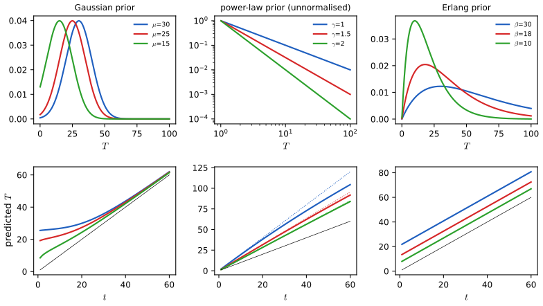
Filling the gap 3.38: posterior medians for the power-law, Erlang and Gaussian priors Supplement pp. 33–36, (S3.13)–(S3.22)
Derivation
Power law \(p(T)\propto T^{-\gamma}\), \(\gamma>0\). \[p(t)\propto\int_t^\infty T^{-(\gamma+1)}\d T=\frac1\gamma t^{-\gamma}\] (S3.16), so for \(T\ge t\) the posterior is \(p(T\given t)=\gamma t^\gamma T^{-(\gamma+1)}\), a Pareto density with minimum \(t\) (this is proper even for the improper prior with \(\gamma\le1\), as the likelihood supplies the factor \(1/T\)). Its tail is \[\Pr(T>T_M\given t)=\int_{T_M}^\infty\gamma t^\gamma T^{-\gamma-1}\d T=(t/T_M)^\gamma\] (S3.18); setting it to \(\frac12\) gives \(T_M=2^{1/\gamma}t\) (S3.18). With \(\gamma=1\) (scale-invariant prior) the rule is "double the observation": 54 for \(t=27\). A multiplier of 1.5, as the book quotes for movie grosses ("about 50% larger"), corresponds to \(\gamma=\log2/\log1.5\approx1.7\); \(\gamma=1.5\) gives 1.59. Such a multiplicative rule is wrong for quantities with a Gaussian prior: with a multiplier of 1.5 a 10-year-old and a 75-year-old would be predicted to live to 15 and 112 (the book's quotation from Griffiths and Tenenbaum).
Erlang \(p(T)\propto Te^{-T/\beta}\). The factor \(T\) cancels the likelihood's \(1/T\): \[p(t)\propto\int_t^\infty e^{-T/\beta}\d T=\beta e^{-t/\beta}\] (S3.20), the posterior is the shifted exponential \(p(T\given t)=\frac1\beta e^{-(T-t)/\beta}\), \(T\ge t\) (S3.21), and \[\Pr(T>T_M\given t)=e^{-(T_M-t)/\beta}=\frac12\] gives \(T_M=t+\beta\log2\) (S3.22): the observation plus a constant (for \(\beta=18\), \(t=27\): 39.5).
Gaussian \(p(T)=\mathcal N(T\given\mu,\sigma^2)\). \[p(T\given t)\propto\frac1T\mathcal N(T\given\mu,\sigma^2)\] on \(T\ge t\) has no closed-form median; solve \(\int_{T_M}^\infty p=\frac12\) numerically (1-d quadrature). For \(t\ll\mu\) the truncation barely matters and \(\hat T\) stays near \(\mu\) (26.8 at \(t=10\) for \(\mu=30,\sigma=10\); the factor \(1/T\) pulls it slightly below \(\mu\)); for \(t\gg\mu\) the posterior is concentrated just above \(t\) with scale \(\sigma^2/(t-\mu)\) and \(\hat T\approx t+\epsilon\), \(\epsilon\approx\frac{\sigma^2\log2}{t-\mu}\) (91.1 at \(t=90\)). All three rules were confirmed by numerical integration (53.7, 42.9, 39.5 for \(t=27\) under \(\gamma=1\), \(\gamma=1.5\), Erlang \(\beta=18\)). \(\square\)
3.2.5 Exchangeability and de Finetti's theorem
p. 72 A sequence is infinitely exchangeable if every finite subsequence has a joint law invariant under permutation, \(p(x_1,\dots,x_n)=p(x_{\pi_1},\dots,x_{\pi_n})\) (3.34). Iid sequences are exchangeable, but not conversely: \(x_i=x_0+z_i\) with a shared background \(x_0\) and iid \(z_i\) is exchangeable with \(\cov(x_i,x_j)=\var x_0\ne0\). De Finetti's theorem says exchangeability is equivalent to a mixture of iid sequences: \[p(x_1,\dots,x_n)=\int\prod_ip(x_i\given\theta)\,p(\theta)\,\d\theta\] (3.35). So a belief in exchangeability implies a parameter, a likelihood and a prior.
Filling the gap 3.4: de Finetti's theorem for binary sequences, with proof p. 72, Theorem 3.2.1
Proof
The book states the theorem without proof. I prove the case \(x_i\in\{0,1\}\) (Diaconis and Freedman, 1980); the general case is an extension. Claim: if \((x_1,x_2,\dots)\) is exchangeable then there is a probability measure \(\mu\) on \([0,1]\) with \[P(x_1=e_1,\dots,x_n=e_n)=\int\theta^{s}(1-\theta)^{n-s}\mu(\d\theta)\], \(s=\sum e_i\). (The converse, that every such mixture is exchangeable, is immediate because the integrand depends on \((e_i)\) only through \(s\).)
Step 1: finite exchangeability is a hypergeometric mixture. Fix \(N\ge n\) and let \(S_N=\sum_{i\le N}x_i\). Conditional on \(S_N=k\), by exchangeability all \(\binom Nk\) arrangements of the \(k\) ones among positions \(1..N\) are equally likely. So the first \(n\) coordinates are the draws, without replacement, of \(n\) balls from an urn with \(k\) ones and \(N-k\) zeros: \(P(e_{1:n}\given S_N=k)=H_N(e_{1:n};k)\) (hypergeometric). Hence \(P(e_{1:n})=\sum_kP(S_N=k)\,H_N(e_{1:n};k)\).
Step 2: sampling without and with replacement are close. Let \(B_N(e_{1:n};k)=\theta^s(1-\theta)^{n-s}\) with \(\theta=k/N\) (draws with replacement). Couple the two: draw \(n\) indices uniformly from \(\{1..N\}\) with replacement; the draws are all distinct with probability at least \(1-\binom n2/N\) (union bound over pairs), and conditionally on being distinct the vector of draws has exactly the law of draws without replacement. Hence \[\sum_{e}|H_N-B_N|\le 2\cdot\binom n2/N=n(n-1)/N\] (total variation bound), uniformly in \(k\).
Step 3: pass to the limit. Let \(F_N\) be the law of \(S_N/N\) on \([0,1]\). Then \[P(e_{1:n})=\int B(e_{1:n};\theta)\,F_N(\d\theta)+r_N\] with \(|r_N|\le n(n-1)/N\), where \(B(e;\theta)=\theta^s(1-\theta)^{n-s}\) is a continuous function of \(\theta\) (here \(k/N\) is replaced by its value in the integrand, an exact identity). By Helly's selection theorem some subsequence of \((F_N)\) converges weakly to a probability measure \(\mu\). Since \(B(e;\cdot)\) is bounded and continuous, along that subsequence \(\int B\,\d F_N\to\int B\,\d\mu\) while \(r_N\to0\), which gives the claim, and \(\mu\) does not depend on \(n\) because the left side does not depend on \(N\). \(\square\)
Example. The beta-Bernoulli sequence of Section 3.2.1 is exchangeable with mixing measure \(\Beta(\breve\alpha,\breve\beta)\): the probability of a sequence with \(s\) ones is \[B(\breve\alpha+s,\breve\beta+n-s)/B(\breve\alpha,\breve\beta)\], invariant under permutations, yet \(P(x_1=x_2=1)\ne P(x_1=1)^2\) because the observations are dependent through \(\theta\) (confirmed numerically).
3.3 Frequentist statistics
pp. 72–73 Frequentist inference represents uncertainty by how a quantity computed from data would vary if the data were redrawn, never by a distribution over parameters. It supplies tools a Bayesian also needs: cross validation, model checking and (Chapter 14) conformal prediction.
3.3.1 Sampling distributions
p. 73 An estimator \(\hat\theta=\hat\Theta(\mathcal D)\) is a function of the data (a decision procedure, Section 34.1.2). Its sampling distribution is the law of \(\hat\Theta(\tilde{\mathcal D})\) for \(\tilde{\mathcal D}\sim\theta^*\) (3.36); with \(S\) simulated datasets it is approximated by \[\frac1S\sum_s\delta(\theta-\hat\Theta(\tilde{\mathcal D}^{(s)}))\] (3.37).
3.3.2 Bootstrap approximation of the sampling distribution
pp. 73–75 If the true \(\theta^*\) were known one would simulate datasets from \(p(x\given\theta^*)\). The parametric bootstrap uses \(\hat\theta=\hat\Theta(\mathcal D)\) instead; the nonparametric bootstrap resamples \(N\) points with replacement, and a resample contains on average a fraction \(1-(1-1/N)^N\to1-e^{-1}\approx0.632\) of the distinct points (gap 4.16; All of Statistics, 8.3). For the Bernoulli MLE both bootstraps are \(\hat\theta^*=\mathrm{Bin}(N,\hat\theta)/N\) in law.
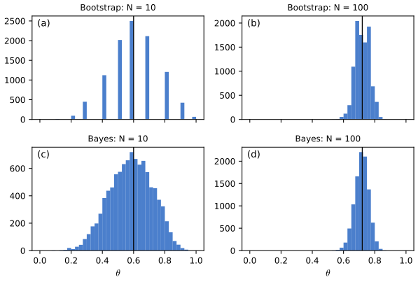
Filling the gap 3.5: why the bootstrap distribution is a "poor man's posterior" (Bernoulli case) p. 75
Derivation
Write \(\hat\theta=N_1/N\in(0,1)\). Bootstrap side. \(N\hat\theta^*\sim\mathrm{Bin}(N,\hat\theta)\), so by the de Moivre–Laplace central limit theorem \[\sqrt N(\hat\theta^*-\hat\theta)/\sqrt{\hat\theta(1-\hat\theta)}\Rightarrow\mathcal N(0,1)\].
Posterior side. The posterior is \(\Beta(\breve\alpha+N_1,\breve\beta+N_0)\). Its log density is \[\ell(\theta)=(N_1+\breve\alpha-1)\log\theta+(N_0+\breve\beta-1)\log(1-\theta)+\mathrm{const}\], maximised at \[\theta_N=\frac{N_1+\breve\alpha-1}{N+\breve\alpha+\breve\beta-2}=\hat\theta+O(1/N)\], with \[-\ell''(\theta_N)=\frac{N}{\hat\theta(1-\hat\theta)}(1+O(1/N))\]. Taylor-expanding to second order with the substitution \(\theta=\theta_N+t/\sqrt N\) gives \[\ell=\ell(\theta_N)-\frac{t^2}{2\hat\theta(1-\hat\theta)}+O(N^{-1/2}|t|^3)\], uniformly on \(|t|\le N^{\epsilon}\), and the tails beyond contribute exponentially little. By Scheffé's lemma the standardised posterior converges in total variation to the same \(\mathcal N(0,1)\). Both distributions are therefore \[\mathcal N(\hat\theta,\hat\theta(1-\hat\theta)/N)\] to first order and differ by terms of relative size \(O(N^{-1/2})\), the skewness visible for \(N=10\).
The two are conceptually different, as the book stresses: the bootstrap varies the data at fixed \(\hat\theta\), the posterior varies \(\theta\) at fixed data. The general statement, for regular parametric models and smooth priors, is the Bernstein–von Mises theorem. \(\square\)
3.3.3 Asymptotic normality of the sampling distribution of the MLE
p. 75 Under regularity conditions \[\sqrt N(\hat\theta-\theta^*)\to\mathcal N(0,F(\theta^*)^{-1})\] (3.38), where \(F\) is the Fisher information matrix (3.40). The proof, by Taylor expansion of the score, is in Result 4.4 of the first volume and in All of Statistics, 9.7; it needs the two facts proved next: the score has mean zero and covariance \(F\), and \(F\) is minus the expected Hessian.
3.3.4 Fisher information matrix
3.3.4.1–3.3.4.2 Definition and the Hessian identity
pp. 76–77 The score is \[\bm s(\theta)=\nabla_\theta\log p(x\given\theta)\] (3.39) and the Fisher information matrix is its second moment \[ F(\theta)=\E_{x\sim p(\cdot\given\theta)}\big[\nabla\log p\,\nabla\log p^\T\big]=-\E\big[\nabla^2\log p(x\given\theta)\big], \tag{3.40, 3.43} \] with \(\E[\bm s]=\bm 0\) (3.44) (Lemma 3.3.1), hence \(F=\cov[\bm s]\). For \(N\) iid observations the expected Hessian of the NLL is \(NF(\theta)\) (3.53).
Filling the gap 3.6: the score lemma and Theorem 3.3.2 in the multi-parameter case, additivity, and reparameterisation pp. 76–77, (3.44)–(3.53), (3.75)
Derivation
Regularity conditions. \(\Theta\) open; the support of \(p(x\given\theta)\) does not depend on \(\theta\); \(\log p\) twice continuously differentiable; derivatives can be passed under the integral sign (for example, \[\sup_{\theta'\text{ near }\theta}\|\partial_\theta^kp(x\given\theta')\|\] integrable for \(k=1,2\)). The book's proof is for one parameter; here is the vector case.
Lemma. From \(\int p(x\given\theta)\,\d x=1\), differentiate in \(\theta_i\): \[0=\int\partial_ip\,\d x=\int(\partial_i\log p)\,p\,\d x=\E[s_i]\], using \(\partial_ip=p\,\partial_i\log p\) (3.46).
Theorem. Differentiate \(0=\int(\partial_i\log p)\,p\,\d x\) in \(\theta_j\): \[0=\int(\partial_{ij}\log p)\,p\,\d x+\int(\partial_i\log p)(\partial_jp)\,\d x=\E[\partial_{ij}\log p]+\E[s_is_j]\], again by \(\partial_jp=p\,s_j\). Hence \(F_{ij}=\E[s_is_j]=-\E[\partial_{ij}\log p]\). Because \(\E[\bm s]=0\), \(F=\cov[\bm s]\) and is positive semidefinite.
Additivity. For independent observations the log likelihood is a sum, so the score of the dataset is the sum of \(N\) iid zero-mean scores and its covariance is \(NF\); likewise the expected Hessian of the NLL is \(NF\) (3.53).
Reparameterisation (used by (3.75) and by Jeffreys' prior). If \(\theta=\theta(\phi)\) is a differentiable invertible map with Jacobian \(J=\partial\theta/\partial\phi\), the chain rule gives \(\nabla_\phi\log p=J^\T\nabla_\theta\log p\), so \(F_\phi=J^\T F_\theta J\) (3.75). (No second-derivative term appears because we use the covariance form; for the Hessian form the extra term has expectation \(\E[\bm s]^\T\partial^2\theta=0\).) \(\square\)
3.3.4.3–3.3.4.5 Examples
pp. 77–78 Binomial. With \(\ell=x\log\theta+(n-x)\log(1-\theta)\): \(s=\frac x\theta-\frac{n-x}{1-\theta}\), \[s'=-\frac x{\theta^2}-\frac{n-x}{(1-\theta)^2}\], and using \(\E x=n\theta\), \[F(\theta)=\frac n\theta+\frac n{1-\theta}=\frac n{\theta(1-\theta)}\] (3.57). Gaussian with parameters \((\mu,v)\), \(v=\sigma^2\): the partials are \(\partial_\mu\ell=(x-\mu)/v\), \[\partial_v\ell=-\frac1{2v}+\frac{(x-\mu)^2}{2v^2}\], \(\partial_\mu^2\ell=-1/v\), \[\partial_v^2\ell=\frac1{2v^2}-\frac{(x-\mu)^2}{v^3}\], \(\partial_\mu\partial_v\ell=-(x-\mu)/v^2\). Taking minus the expectation, \(F(\mu,v)=\diag\big(\frac1v,\frac1{2v^2}\big)\) (3.62); the book's displayed entries omit the minus signs of \(-\E[\partial^2\ell]\) but the matrix is right. Logistic regression with an \(\ell_2\) penalty: \[\mathcal L(\bm w)=-\bm w^\T\bm X^\T\bm y+\sum_n\log(1+e^{\bm w^\T\bm x_n})+\frac\lambda2\bm w^\T\bm w\] (3.63), gradient \(\bm X^\T(\bm s-\bm y)+\lambda\bm w\) (3.64) with \(s_n=\sigma(\bm w^\T\bm x_n)\), and Hessian \(\bm X^\T\Lambda\bm X+\lambda\bm I\) with \(\Lambda_{nn}=s_n(1-s_n)\) (3.65)–(3.66). The Hessian does not depend on \(\bm y\), so it equals its expectation; strictly it is the Fisher information of the penalised objective (the penalty adds \(\lambda\bm I\)). Each statement was confirmed numerically.
3.3.4.6 FIM for the exponential family
p. 79 For \[p(x\given\bm\eta)=h(x)\exp(\bm\eta^\T\bm T(x)-A(\bm\eta))\]: \(\nabla A=\E[\bm T]=\bm m\) (3.67), \(\nabla_\eta\log p=\bm T-\bm m\) (3.68), \(F_\eta=\cov[\bm T]\) (3.72), and in the moment parameters \(F_m=F_\eta^{-1}\) (3.80).
Filling the gap 3.7: the exponential-family Fisher information in natural and moment parameters p. 79, (3.67)–(3.80)
Derivation
Moments from the log partition. Normalisation \[\int h\,e^{\bm\eta^\T\bm T-A(\bm\eta)}\,\d x=1\] means \[A(\bm\eta)=\log\int h\,e^{\bm\eta^\T\bm T}\,\d x\]. Differentiating under the integral, \[\nabla A=\frac{\int\bm Th\,e^{\bm\eta^\T\bm T}}{\int h\,e^{\bm\eta^\T\bm T}}=\E[\bm T]\], and differentiating again, \[\nabla^2A=\E[\bm T\bm T^\T]-\E[\bm T]\E[\bm T]^\T=\cov[\bm T]\] (derivatives under the integral are legitimate in the interior of the natural parameter space, where the moment generating function is analytic).
Fisher information. The score is \(\bm T-\E\bm T\) (3.68), so \[F_\eta=\E[(\bm T-\bm m)(\bm T-\bm m)^\T]=\cov[\bm T]=\nabla^2A\] (3.69)–(3.72); equivalently \(-\E[\nabla^2\log p]=\nabla^2A\), consistent with the Hessian identity of gap 3.6.
Moment parameters. The map \(\bm\eta\mapsto\bm m=\nabla A(\bm\eta)\) has Jacobian \[\partial\bm m/\partial\bm\eta=\nabla^2A=F_\eta\] (the book derives the same thing by the log-derivative trick (3.76)–(3.78)). It is invertible because \(F_\eta\succ0\) for a minimal family. So \(\partial\bm\eta/\partial\bm m=F_\eta^{-1}\) (3.79) and, by the reparameterisation rule of gap 3.6, \[F_m=(\partial\bm\eta/\partial\bm m)^\T F_\eta(\partial\bm\eta/\partial\bm m)=F_\eta^{-1}F_\eta F_\eta^{-1}=F_\eta^{-1}=\cov[\bm T]^{-1}\] (3.80).
Checks. Bernoulli: \(\eta=\log\frac\theta{1-\theta}\), \(T=x\), \(F_\eta=\theta(1-\theta)\), \(m=\theta\), \(F_m=\frac1{\theta(1-\theta)}\), which is (3.57) with \(n=1\). Poisson: \(\eta=\log\lambda\), \(T=x\), \(F_\eta=\lambda\), \(m=\lambda\), \(F_m=1/\lambda\). \(\square\)
3.3.5 Counterintuitive properties of frequentist statistics
3.3.5.1 Confidence intervals
pp. 80–81 A \(100(1-\alpha)\%\) confidence interval is a random interval \(I(\tilde{\mathcal D})\) with \[\Pr(\theta\in I(\tilde{\mathcal D})\given\tilde{\mathcal D}\sim\theta)=1-\alpha\] (3.81): a statement about repeated datasets, not about the interval at hand. In Berger's example, two draws \(y_1,y_2\) from \(p(y)=\frac12\) on \(\{\theta,\theta+1\}\) and the interval \([m,m]\), \(m=\min(y_1,y_2)\), covers \(\theta=39\) with probability \(3/4\) over the four equally likely outcomes (3.83)–(3.85); yet on observing \((39,40)\) the parameter is certainly 39. The full worked example, and the failures of the Wald interval, are in Filling the gap 4.18.
3.3.5.2 p-values
pp. 81–82 The p-value is \[\mathrm{pval}(t(\mathcal D))=\Pr(t(\tilde{\mathcal D})\ge t(\mathcal D)\given\tilde{\mathcal D}\sim H_0)\] (3.86). "If \(H_0\) is true the statistic would probably not occur; it did occur; so \(H_0\) is probably false" is invalid reasoning (the Congress example), because \(p(H_0\given\mathcal D)\) needs \(p(\mathcal D\given H_1)\) and the prior: \[p(H_0\given\mathcal D)=\frac{p(\mathcal D\given H_0)p(H_0)}{p(\mathcal D\given H_0)p(H_0)+p(\mathcal D\given H_1)p(H_1)}\] (3.87), which for equal priors is \(\mathrm{LR}/(\mathrm{LR}+1)\) with \[\mathrm{LR}=p(\mathcal D\given H_0)/p(\mathcal D\given H_1)\] (3.88). In the Congress example \(p(\mathcal D\given H_1)=0\) so \(\mathrm{LR}=\infty\) and \(p(H_0\given\mathcal D)=1\). See All of Statistics, 10.2.
Filling the gap 3.8: how small can \(p(H_0\given\mathcal D)\) be when \(p=0.05\)? pp. 81–82, (3.86)–(3.88)
Derivation
A calibration due to Sellke, Bayarri and Berger (2001) makes the book's warning quantitative. Under \(H_0\) the p-value is uniform on \((0,1)\), with density \(f_0(p)=1\). Take as alternatives the family \(f_\xi(p)=\xi p^{\xi-1}\), \(0<\xi\le1\) (densities of Beta\((\xi,1)\) that put more mass near \(p=0\); \(\xi=1\) is \(H_0\)). The Bayes factor in favour of \(H_0\) against any mixture of this family is at least the minimum over \(\xi\) of \(f_0/f_\xi\), i.e. at least \(1/\sup_\xi f_\xi(p)\). Maximise \(g(\xi)=\xi p^{\xi-1}\): \(\log g=\log\xi+(\xi-1)\log p\), derivative \(\frac1\xi+\log p=0\), so \(\xi^*=-1/\log p\) (in \((0,1)\) iff \(p<1/e\)). Then \(p^{\xi^*}=e^{\xi^*\log p}=e^{-1}\) and \(g(\xi^*)=\xi^*e^{-1}p^{-1}=-1/(e\,p\log p)\). Hence \[ \mathrm{LR}=\frac{p(\mathcal D\given H_0)}{p(\mathcal D\given H_1)}\ \ge\ -e\,p\log p\qquad(p<1/e),\] and with equal prior odds \[p(H_0\given\mathcal D)\ge\big(1+(-e\,p\log p)^{-1}\big)^{-1}\] by (3.88) (the right side is increasing in the Bayes factor). For \(p=0.05\): \(-e\cdot0.05\cdot\log0.05=0.407\) and \(p(H_0\given\mathcal D)\ge0.289\). So a result at the 5% "significance" level leaves \(H_0\) at least 29% probable under the most favourable alternative family: the p-value overstates the evidence against the null. For \(p=0.01\) the bound is \(0.111\). \(\square\)
3.3.5.3–3.3.6 Discussion; why isn't everyone a Bayesian?
pp. 82–83 The difficulties share one cause: frequentist inference is not conditional on the data actually observed. The book quotes Berger (1985) and Efron (1986) on this, and Rubin (1984): be Bayesian in principle and calibrated in practice, using model checking (Section 3.9) to test the assumptions that Bayesian inference takes on trust. The remaining obstacles, computation and the reliance on modelling assumptions, are what the rest of the chapter and Part II address. Bayesian alternatives to "cookie-cutter" tests are in Section 3.10.
3.4 Conjugate priors
pp. 83–99 A family \(\mathcal F\) of priors is conjugate to a likelihood if the posterior is again in \(\mathcal F\). If \(\mathcal F\) is exponential, the update is closed form and can serve as a subroutine inside larger algorithms.
3.4.1–3.4.2 The binomial and multinomial models
pp. 84–85 The binomial case is Section 3.2.1. For a categorical variable with counts \(N_c\) the likelihood is \(\prod_c\theta_c^{N_c}\) (3.89) (the multinomial differs by a constant factor (3.90)), the conjugate prior is \(\Dir(\bm\theta\given\breve{\bm\alpha})\) and the posterior is \(\Dir(\bm\theta\given\breve{\bm\alpha}+\bm N)\) (3.91)–(3.92), with mode \[(N_k+\breve\alpha_k-1)/\sum_{k'}(N_{k'}+\breve\alpha_{k'}-1)\] (3.93) and marginal likelihood \[p(\mathcal D)=B(\bm N+\bm\alpha)/B(\bm\alpha)=\frac{\Gamma(\sum_k\alpha_k)}{\Gamma(N+\sum_k\alpha_k)}\prod_k\frac{\Gamma(N_k+\alpha_k)}{\Gamma(\alpha_k)}\] (3.94)–(3.96). A symmetric prior \(\alpha_k=\breve\alpha/K\) has \(\E\theta_k=1/K\) and \(\var\theta_k=\frac{K-1}{K^2(\breve\alpha+1)}\). All proved in Filling the gap 4.11.
3.4.3 The univariate Gaussian model
3.4.3.1 Posterior of \(\mu\) given \(\sigma^2\)
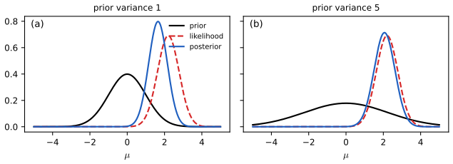
pp. 85–86 With likelihood \[\propto\exp(-\frac1{2\sigma^2}\sum_n(y_n-\mu)^2)\] (3.97) and prior \(\mathcal N(\mu\given\breve m,\breve\tau^2)\), the posterior is \(\mathcal N(\hat m,\hat\tau^2)\) with \[ \hat\tau^2=\Big(\frac N{\sigma^2}+\frac1{\breve\tau^2}\Big)^{-1},\qquad\hat m=\hat\tau^2\Big(\frac{\breve m}{\breve\tau^2}+\frac{N\bar y}{\sigma^2}\Big) \tag{3.99, 3.100} \] or, in precisions \(\lambda=1/\sigma^2\), \(\breve\lambda=1/\breve\tau^2\): \(\hat\lambda=\breve\lambda+N\lambda\), \[\hat m=\frac{N\lambda\bar y+\breve\lambda\breve m}{\hat\lambda}\] (3.102)–(3.103). For one observation \[\hat m=\breve m+\frac\lambda{\hat\lambda}(y-\breve m)=y-w(y-\breve m)\] with \(w=\breve\lambda/\hat\lambda\): a shrinkage estimate (3.104)–(3.107). Proof: Filling the gap 4.12.
3.4.3.2 Posterior of \(\sigma^2\) given \(\mu\)
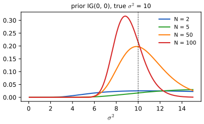
pp. 86–88 The likelihood is \[(\sigma^2)^{-N/2}\exp(-\frac1{2\sigma^2}\sum_n(y_n-\mu)^2)\] (3.108); the conjugate prior is inverse gamma \(\mathrm{IG}(\sigma^2\given\breve a,\breve b)\) (3.109), giving \[\mathrm{IG}(\breve a+N/2,\ \breve b+\frac12\sum_n(y_n-\mu)^2)\] (3.110)–(3.112). The scaled inverse chi-squared \[\chi^{-2}(\sigma^2\given\nu,\tau^2)=\mathrm{IG}(\nu/2,\nu\tau^2/2)\] (3.113) separates strength (\(\nu\), degrees of freedom) from location (\(\tau^2\)): the posterior is \(\chi^{-2}(\hat\nu,\hat\tau^2)\), \(\hat\nu=\breve\nu+N\), \[\hat\nu\hat\tau^2=\breve\nu\breve\tau^2+\sum_n(y_n-\mu)^2\] (3.114)–(3.116): prior and data sums of squares add.
3.4.3.3 Posterior of \(\mu\) and \(\sigma^2\): conjugate prior
pp. 88–89 The joint conjugate prior is the normal inverse chi-squared \[ \NIX(\mu,\sigma^2\given\breve m,\breve\kappa,\breve\nu,\breve\tau^2)=\mathcal N(\mu\given\breve m,\sigma^2/\breve\kappa)\,\chi^{-2}(\sigma^2\given\breve\nu,\breve\tau^2)\propto(\sigma^2)^{-(\breve\nu+3)/2}\exp\Big(-\frac{\breve\nu\breve\tau^2+\breve\kappa(\mu-\breve m)^2}{2\sigma^2}\Big), \tag{3.118--3.119} \] and the posterior is \(\NIX(\hat m,\hat\kappa,\hat\nu,\hat\tau^2)\) with \[ \hat m=\frac{\breve\kappa\breve m+N\bar y}{\hat\kappa},\quad\hat\kappa=\breve\kappa+N,\quad\hat\nu=\breve\nu+N,\quad\hat\nu\hat\tau^2=\breve\nu\breve\tau^2+\sum_n(y_n-\bar y)^2+\frac{N\breve\kappa}{\breve\kappa+N}(\breve m-\bar y)^2. \tag{3.121--3.124} \] Marginally \[\sigma^2\given\mathcal D\sim\chi^{-2}(\hat\nu,\hat\tau^2)\] with mean \(\frac{\hat\nu}{\hat\nu-2}\hat\tau^2\) (3.125) and \[\mu\given\mathcal D\sim T(\hat m,\hat\tau^2/\hat\kappa,\hat\nu)\] (3.126).
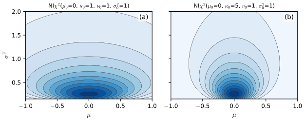
Filling the gap 3.9: the NIX posterior, its marginals, the scale-mixture identity and the Jeffreys limit pp. 86–90, (3.110)–(3.134)
Derivation
Completing the square. Let \(S=\sum_n(y_n-\bar y)^2\), so \(\sum_n(y_n-\mu)^2=S+N(\bar y-\mu)^2\). For any \(\breve m,\bar y\) with weights \(\breve\kappa,N\) and \(\hat\kappa=\breve\kappa+N\), \[ \breve\kappa(\mu-\breve m)^2+N(\mu-\bar y)^2=\hat\kappa(\mu-\hat m)^2+\frac{\breve\kappa N}{\hat\kappa}(\breve m-\bar y)^2,\qquad\hat m=\frac{\breve\kappa\breve m+N\bar y}{\hat\kappa}. \] (Expand both sides: the coefficient of \(\mu^2\) is \(\hat\kappa\), of \(\mu\) is \(-2(\breve\kappa\breve m+N\bar y)\), and the constants agree because \[\breve\kappa\breve m^2+N\bar y^2-\hat\kappa\hat m^2=\frac{\breve\kappa N}{\hat\kappa}(\breve m-\bar y)^2\].)
Posterior. Multiply the likelihood \[(\sigma^2)^{-N/2}\exp(-\frac{S+N(\bar y-\mu)^2}{2\sigma^2})\] by the prior kernel (3.119): the power of \(\sigma^2\) is \(-\frac{N+\breve\nu+3}2=-\frac{\hat\nu+3}2\) and the exponent is \[-\frac1{2\sigma^2}\big[\breve\nu\breve\tau^2+S+\breve\kappa(\mu-\breve m)^2+N(\mu-\bar y)^2\big]=-\frac1{2\sigma^2}\big[\hat\nu\hat\tau^2+\hat\kappa(\mu-\hat m)^2\big]\] with \(\hat\nu\hat\tau^2\) as in (3.124). This is the kernel of \(\NIX(\hat m,\hat\kappa,\hat\nu,\hat\tau^2)\).
Marginal of \(\sigma^2\). \[\int\mathcal N(\mu\given\hat m,\sigma^2/\hat\kappa)\,\d\mu=1\], so integrating the \(\mu\)-factor leaves \[\chi^{-2}(\sigma^2\given\hat\nu,\hat\tau^2)=\mathrm{IG}(\hat\nu/2,\hat\nu\hat\tau^2/2)\], whose mean is \[\frac{\hat\nu\hat\tau^2/2}{\hat\nu/2-1}=\frac{\hat\nu}{\hat\nu-2}\hat\tau^2\] for \(\hat\nu>2\) (3.125).
Marginal of \(\mu\) (scale-mixture identity). Integrating the kernel over \(\sigma^2\) with \(u=1/\sigma^2\) (so \(\d\sigma^2=u^{-2}\d u\)): \[\int_0^\infty u^{(\hat\nu+3)/2-2}e^{-uQ/2}\,\d u=\Gamma\big(\tfrac{\hat\nu+1}2\big)(Q/2)^{-(\hat\nu+1)/2}\] with \(Q=\hat\nu\hat\tau^2+\hat\kappa(\mu-\hat m)^2\). Hence \[p(\mu\given\mathcal D)\propto\big(1+\frac{\hat\kappa(\mu-\hat m)^2}{\hat\nu\hat\tau^2}\big)^{-(\hat\nu+1)/2}\], the Student density \(T(\hat m,\hat\tau^2/\hat\kappa,\hat\nu)\) (3.126). The same integral shows: if \(y\given\sigma^2\sim\mathcal N(m,c\sigma^2)\) and \(\sigma^2\sim\chi^{-2}(\nu,s^2)\) then \(y\sim T(m,cs^2,\nu)\), which was used in gap 3.2. The Student law is a Gaussian scale mixture, hence heavier tailed.
Jeffreys limit. The prior kernel with \(\breve\kappa=0\), \(\breve\nu=-1\), \(\breve\nu\breve\tau^2=0\) is \((\sigma^2)^{-(-1+3)/2}=\sigma^{-2}\), flat in \(\mu\): the improper prior (3.127), obtained formally as a limit (3.128). The update then gives \(\hat m=\bar y\), \(\hat\kappa=N\), \(\hat\nu=N-1\), \(\hat\nu\hat\tau^2=S\) i.e. \(\hat\tau^2=s^2=S/(N-1)\) (3.129)–(3.130), with \(s^2=\frac N{N-1}\hat\sigma^2_{\rm mle}\). So \(\mu\given\mathcal D\sim T(\bar y,s^2/N,N-1)\) (3.131); the variance of a Student with \(\nu\) degrees of freedom and scale \(\tau^2\) is \(\frac\nu{\nu-2}\tau^2\) (for \(\nu>2\), i.e. \(N>3\)), giving \[\var[\mu\given\mathcal D]=\frac{N-1}{N-3}\frac{s^2}N\to s^2/N\] (3.132) and the standard error \(s/\sqrt N\) (3.133). The 95% credible interval is \[\bar y\pm t_{N-1,0.975}\,s/\sqrt N\approx\bar y\pm2s/\sqrt N\] (3.134), identical to the classical t confidence interval, because the pivot \(\sqrt N(\mu-\bar y)/s\) has the t distribution both over repeated samples (given \(\mu\)) and over the posterior (given the data). This is the sense in which the Bayesian and frequentist answers coincide for the Gaussian mean under the Jeffreys prior. (All formulas confirmed against two-dimensional quadrature.) \(\square\)
3.4.3.4 Posterior of \(\mu\) and \(\sigma^2\): uninformative prior
pp. 89–90 Covered in gap 3.9: the Jeffreys prior \(p(\mu,\sigma^2)\propto\sigma^{-2}\) (see Section 3.5.2.3 for the sense in which it is Jeffreys) is the \(\NIX\) limit with \(\breve\nu=-1\), and the posterior of the mean is the t law above.
3.4.4 The multivariate Gaussian model
3.4.4.1 Posterior of \(\bm\mu\) given \(\Sigma\)
pp. 90–91 With \(\bm\mu\sim\mathcal N(\breve{\bm m},\breve V)\): \(\hat V^{-1}=\breve V^{-1}+N\Sigma^{-1}\), \[\hat{\bm m}=\hat V(\Sigma^{-1}N\bar{\bm y}+\breve V^{-1}\breve{\bm m})\] (3.136)–(3.138): gap 4.12.
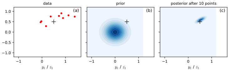
3.4.4.2–3.4.4.3 Posterior of \(\Sigma\), and of \((\bm\mu,\Sigma)\)
pp. 91–96 With scatter matrix \[S_\mu=\sum_n(\bm y_n-\bm\mu)(\bm y_n-\bm\mu)^\T\] the likelihood is \[\propto|\Sigma|^{-N/2}\exp(-\frac12\Tr(S_\mu\Sigma^{-1}))\] (3.139)–(3.140); the conjugate prior is inverse Wishart \[\IW(\Sigma\given\breve\Psi^{-1},\breve\nu)\propto|\Sigma|^{-(\breve\nu+D+1)/2}\exp(-\frac12\Tr(\breve\Psi\Sigma^{-1}))\] (3.141) (the book's argument reads \(\breve\Psi^{-1}\); the scatter matrix is \(\breve\Psi\)), and the posterior is \(\IW(\hat\Psi,\hat\nu)\) with \(\hat\nu=\breve\nu+N\), \(\hat\Psi=\breve\Psi+S_\mu\) (3.144)–(3.146). When both mean and covariance are unknown the likelihood couples them (3.148)–(3.151), so the factorised prior (3.152) is only conditionally conjugate (Figure 3.9a); the fully conjugate prior is the normal inverse Wishart \[\NIW(\bm\mu,\Sigma\given\breve{\bm m},\breve\kappa,\breve\nu,\breve\Psi)=\mathcal N(\bm\mu\given\breve{\bm m},\Sigma/\breve\kappa)\,\IW(\Sigma\given\breve\Psi^{-1},\breve\nu)\] (3.153)–(3.155), with posterior \[ \hat{\bm m}=\frac{\breve\kappa\breve{\bm m}+N\bar{\bm y}}{\hat\kappa},\quad\hat\kappa=\breve\kappa+N,\quad\hat\nu=\breve\nu+N,\quad\hat\Psi=\breve\Psi+S+\frac{\breve\kappa N}{\hat\kappa}(\bar{\bm y}-\breve{\bm m})(\bar{\bm y}-\breve{\bm m})^\T \tag{3.168--3.171} \] (equivalently \[\breve\Psi+\bm Y^\T\bm Y+\breve\kappa\breve{\bm m}\breve{\bm m}^\T-\hat\kappa\hat{\bm m}\hat{\bm m}^\T\], (3.172)). Marginally \[\Sigma\given\mathcal D\sim\IW(\hat\Psi,\hat\nu)\] (3.174) and \[\bm\mu\given\mathcal D\sim T(\hat{\bm m},\hat\Psi/(\hat\kappa\hat\nu'),\hat\nu')\], \(\hat\nu'=\hat\nu-D+1\) (3.175). The mode is \(\hat{\bm\mu}=\hat{\bm m}\), \(\hat\Sigma=\hat\Psi/(\hat\nu+D+2)\) (3.179)–(3.180), and the predictive is \[T\big(\hat{\bm m},\hat\Psi(\hat\kappa+1)/(\hat\kappa\hat\nu'),\hat\nu'\big)\] (3.182). A prior sample size for the covariance is \(\breve N_0=\breve\nu+D+1\).
Filling the gap 3.10: IW and NIW posteriors, marginals, mode and predictive pp. 91–96, (3.142)–(3.182)
Derivation
Inverse Wishart update. Multiplying (3.139) by (3.141) the power of \(|\Sigma|\) is \(-\frac{N+\breve\nu+D+1}2=-\frac{\hat\nu+D+1}2\) and the exponent is \(-\frac12\Tr[(\breve\Psi+S_\mu)\Sigma^{-1}]\), the kernel of \(\IW(\breve\Psi+S_\mu,\breve\nu+N)\).
Two matrix identities. (i) For every \(\bm\mu\): \[\sum_n(\bm y_n-\bm\mu)^\T\Sigma^{-1}(\bm y_n-\bm\mu)=\Tr(\Sigma^{-1}S)+N(\bar{\bm y}-\bm\mu)^\T\Sigma^{-1}(\bar{\bm y}-\bm\mu)\], with \[S=\sum_n(\bm y_n-\bar{\bm y})(\bm y_n-\bar{\bm y})^\T\]: split \[\bm y_n-\bm\mu=(\bm y_n-\bar{\bm y})+(\bar{\bm y}-\bm\mu)\]; the cross term is \[2(\sum_n(\bm y_n-\bar{\bm y}))^\T\Sigma^{-1}(\bar{\bm y}-\bm\mu)=0\] (3.148). (ii) For weights \(\breve\kappa,N\): \[ \breve\kappa(\bm\mu-\breve{\bm m})(\bm\mu-\breve{\bm m})^\T+N(\bm\mu-\bar{\bm y})(\bm\mu-\bar{\bm y})^\T=\hat\kappa(\bm\mu-\hat{\bm m})(\bm\mu-\hat{\bm m})^\T+\frac{\breve\kappa N}{\hat\kappa}(\bar{\bm y}-\breve{\bm m})(\bar{\bm y}-\breve{\bm m})^\T, \] the matrix version of the one-dimensional identity of gap 3.9 (only the trace against \(\Sigma^{-1}\) is used, so the scalar identity applied to \(\bm u^\T\Sigma^{-1}\bm u\) suffices). The two-sided identity (3.172) follows from \(S=\bm Y^\T\bm Y-N\bar{\bm y}\bar{\bm y}^\T\) (3.156).
NIW update. The powers of \(|\Sigma|\): likelihood \(-N/2\), the Gaussian factor of the prior \(-1/2\), the IW factor \(-(\breve\nu+D+1)/2\), total \(-(\hat\nu+D+2)/2\) (the book's (3.166) drops the minus sign). The exponent is \[-\frac12\Tr\{\Sigma^{-1}[\breve\Psi+S+\breve\kappa(\bm\mu-\breve{\bm m})(\ldots)^\T+N(\bm\mu-\bar{\bm y})(\ldots)^\T]\}\], which by (ii) equals \[-\frac12\Tr\{\Sigma^{-1}[\hat\Psi+\hat\kappa(\bm\mu-\hat{\bm m})(\bm\mu-\hat{\bm m})^\T]\}\] with \(\hat\Psi\) as in (3.171). Since \[\mathcal N(\bm\mu\given\hat{\bm m},\Sigma/\hat\kappa)\IW(\Sigma\given\hat\Psi^{-1},\hat\nu)\] has exactly this kernel (powers \(-\frac12-\frac{\hat\nu+D+1}2\)), the posterior is NIW. The \(\Sigma\)-marginal (3.174) follows because the Gaussian factor integrates to one.
Marginal of \(\bm\mu\). With \(\bm v=\bm\mu-\hat{\bm m}\): \[p(\bm\mu\given\mathcal D)\propto\int|\Sigma|^{-(\hat\nu+D+2)/2}\exp\{-\frac12\Tr[\Sigma^{-1}(\hat\Psi+\hat\kappa\bm v\bm v^\T)]\}\,\d\Sigma\]. The integrand is the kernel of \[\IW(\hat\Psi+\hat\kappa\bm v\bm v^\T,\hat\nu+1)\] (power \(-\frac{(\hat\nu+1)+D+1}2\)), whose normaliser is proportional to \[|\hat\Psi+\hat\kappa\bm v\bm v^\T|^{(\hat\nu+1)/2}\] (the \(\IW(\Psi,\nu)\) density integrates to a constant times \(|\Psi|^{\nu/2}\)). By the matrix determinant lemma \[|\hat\Psi+\hat\kappa\bm v\bm v^\T|=|\hat\Psi|(1+\hat\kappa\bm v^\T\hat\Psi^{-1}\bm v)\]. Hence \[p(\bm\mu\given\mathcal D)\propto(1+\hat\kappa\bm v^\T\hat\Psi^{-1}\bm v)^{-(\hat\nu+1)/2}\], the multivariate Student \[T(\hat{\bm m},\hat\Psi/(\hat\kappa\hat\nu'),\hat\nu')\] with \(\hat\nu'+D=\hat\nu+1\), i.e. \(\hat\nu'=\hat\nu-D+1\) (3.175).
Predictive. Given \(\Sigma\), \(\bm y=\bm\mu+\bm\varepsilon\) with \[\bm\mu\sim\mathcal N(\hat{\bm m},\Sigma/\hat\kappa)\] and \(\bm\varepsilon\sim\mathcal N(0,\Sigma)\) independent, so \[\bm y\given\Sigma\sim\mathcal N(\hat{\bm m},\frac{\hat\kappa+1}{\hat\kappa}\Sigma)\]. This is the previous marginal calculation with \(\hat\kappa\) replaced by \(\hat\kappa/(\hat\kappa+1)\), giving \[T\big(\hat{\bm m},\hat\Psi\frac{\hat\kappa+1}{\hat\kappa\hat\nu'},\hat\nu'\big)\] (3.182).
Mode. The density in \((\bm\mu,\Sigma)\) is maximised at \(\bm\mu=\hat{\bm m}\) for every \(\Sigma\) (the Gaussian factor peaks at its mean). Then \[-2\log p=(\hat\nu+D+2)\log|\Sigma|+\Tr(\hat\Psi\Sigma^{-1})+\mathrm{const}\]; its derivative in \(\Sigma\) is \[(\hat\nu+D+2)\Sigma^{-1}-\Sigma^{-1}\hat\Psi\Sigma^{-1}\] (the book's (3.178) writes it for \(\partial\log p\) but has the factor of \(-2\) of the objective). Setting it to zero: \(\Sigma=\hat\Psi/(\hat\nu+D+2)\) (3.180); the book's sentence says \(\hat\Psi\) itself is the maximiser, which is a slip, since the correct statement is the scaled matrix of (3.180). Uniqueness: in the precision \(\Lambda=\Sigma^{-1}\) the objective \[-(\hat\nu+D+2)\log|\Lambda|+\Tr(\hat\Psi\Lambda)\] is strictly convex on the positive definite cone. The mode of a density depends on the parameterisation: this is the mode of the density with respect to \(\d\Sigma\) (the MAP of \(\Sigma\) alone differs, with \(\hat\nu+D+1\) in the denominator, as in gap 4.5 of the first volume). \(\square\)
3.4.5 The exponential family model
pp. 96–98 Because a conjugate posterior has the same number of parameters as the prior, the likelihood needs fixed-size sufficient statistics; the Pitman–Koopman–Darmois theorem (Diaconis and Ylvisaker, 1979, cited by the book) says this forces an exponential family (with exceptions such as the uniform, below). With likelihood \[p(\mathcal D\given\bm\eta)=h(\mathcal D)\exp(\bm\eta^\T\bm s(\mathcal D)-NA(\bm\eta))\] (3.183) the prior \[p(\bm\eta)=Z(\breve{\bm\tau},\breve\nu)^{-1}\exp(\breve{\bm\tau}^\T\bm\eta-\breve\nu A(\bm\eta))\] (3.184) has posterior parameters \[\hat{\bm\tau}=\breve{\bm\tau}+\bm s(\mathcal D)\], \(\hat\nu=\breve\nu+N\) (3.188)–(3.189); the marginal likelihood is \[p(\mathcal D)=Z(\hat{\bm\tau},\hat\nu)h(\mathcal D)/Z(\breve{\bm\tau},\breve\nu)\] (3.193) and the predictive \[p(\mathcal D'\given\mathcal D)=h(\mathcal D')Z(\breve{\bm\tau}+\bm s(\mathcal D)+\bm s(\mathcal D'),\breve\nu+N+N')/Z(\breve{\bm\tau}+\bm s(\mathcal D),\breve\nu+N)\] (3.196). The Bernoulli example (3.197)–(3.206) recovers the beta model with \(\alpha=\tau_0+1\), \(\beta=\nu_0-\tau_0+1\).
Filling the gap 3.11: exponential-family conjugacy, the predictive as a ratio of normalisers, and the uniform–Pareto exception pp. 96–98, footnote 6
Derivation
Update. Multiplying (3.183) by the prior, \[p(\bm\eta\given\mathcal D)\propto\exp((\breve{\bm\tau}+\bm s)^\T\bm\eta-(\breve\nu+N)A(\bm\eta))\], which is (3.187) with the normaliser \[Z(\hat{\bm\tau},\hat\nu)=\int\exp(\hat{\bm\tau}^\T\bm\eta-\hat\nu A)\,\d\bm\eta\], finite when the prior is proper and the data statistics lie in the interior of the support. Equating normalisers gives \[Z(\hat{\bm\tau},\hat\nu)=Z(\breve{\bm\tau},\breve\nu)h(\mathcal D)/p(\mathcal D)\] (3.190), hence (3.193).
Posterior mean. Since \(\nabla A(\bm\eta)=\bm m\), the prior mean of the moment parameter is \(\breve{\bm\tau}/\breve\nu\) (this is the sense of "\(\E[\eta]\)" in (3.191); the identity \[\E[\nabla A(\bm\eta)]=\breve{\bm\tau}/\breve\nu\] follows by integrating \(\nabla_\eta\) of the prior density, which vanishes on the boundary: \[0=\int(\breve{\bm\tau}-\breve\nu\nabla A)p(\bm\eta)\,\d\bm\eta\]). Then \[\E[\bm m\given\mathcal D]=\frac{\breve{\bm\tau}+\bm s}{\breve\nu+N}=\lambda\frac{\breve{\bm\tau}}{\breve\nu}+(1-\lambda)\frac{\bm s}N\], \(\lambda=\frac{\breve\nu}{\breve\nu+N}\): a convex combination of the prior mean and the MLE \(\bm s/N\) (3.191)–(3.192).
Predictive. \[p(\mathcal D'\given\mathcal D)=\int h(\mathcal D')e^{\bm\eta^\T\bm s'-N'A}\frac{e^{\hat{\bm\tau}^\T\bm\eta-\hat\nu A}}{Z(\hat{\bm\tau},\hat\nu)}\,\d\bm\eta=\frac{h(\mathcal D')Z(\hat{\bm\tau}+\bm s',\hat\nu+N')}{Z(\hat{\bm\tau},\hat\nu)}\] (3.194)–(3.196).
Example (verified numerically). Poisson: \(A=e^\eta\), \(Z(\tau,\nu)=\Gamma(\tau)/\nu^\tau\) (a gamma prior), and the predictive for one new count \(x\) is \[\frac1{x!}\frac{\Gamma(\hat\tau+x)}{\Gamma(\hat\tau)}\frac{\hat\nu^{\hat\tau}}{(\hat\nu+1)^{\hat\tau+x}}\], the negative binomial.
Footnote 6: uniform and Pareto. For \(x_n\sim\mathrm{Unif}(0,\theta)\) the likelihood is \(\theta^{-N}\mathbb 1[\theta\ge m]\), \(m=\max_nx_n\): fixed-size sufficient statistics \((N,m)\) without being an exponential family (its support depends on \(\theta\), so Pitman–Koopman–Darmois does not apply). With the Pareto prior \[\propto\theta^{-(\kappa+1)}\mathbb 1[\theta\ge\theta_0]\] the posterior is \[\propto\theta^{-(\kappa+N+1)}\mathbb 1[\theta\ge\max(\theta_0,m)]\], i.e. \(\mathrm{Pareto}(\max(\theta_0,m),\kappa+N)\). \(\square\)
3.4.6 Beyond conjugate priors
3.4.6.1 Mixtures of conjugate priors
pp. 99–100 A mixture \(p(\theta)=\sum_kp(h=k)p(\theta\given h=k)\) (3.208) of conjugate priors is conjugate: the posterior is \[\sum_kp(h=k\given\mathcal D)p(\theta\given\mathcal D,h=k)\] with weights \(\propto p(h=k)p(\mathcal D\given h=k)\) (3.209)–(3.210) (gap 4.10). For the casino prior \(0.5\,\Beta(20,20)+0.5\,\Beta(30,10)\) and 20 heads, 10 tails the posterior is \(0.346\,\Beta(40,30)+0.654\,\Beta(50,20)\) (3.211), with \(\Pr(\theta>0.5\given\mathcal D)=0.9604\) (3.212), against 0.8858 under a single Beta(20,20) prior (confirmed numerically).
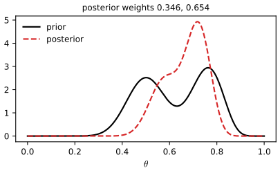
3.4.6.2 Robust (heavy-tailed) priors
p. 100 Sensitivity (robustness) analysis asks how much the prior drives the posterior. In Berger's example, \(x\sim\mathcal N(\theta,1)\), \(x=5\) observed, prior median 0 and probability \(\frac14\) in each of \((-\infty,-1),(-1,0),(0,1),(1,\infty)\): a Gaussian prior with those quartiles gives posterior mean 3.43, a Cauchy prior with the same quartiles about 4.6. Heavy-tailed priors let strong data override the prior.
Filling the gap 3.12: the Gaussian and Cauchy priors of Berger's example p. 100
Derivation
Gaussian. Quartiles at \(\pm1\) require \(\Phi(1/s)=\frac34\), so \(s=1/\Phi^{-1}(0.75)=1/0.6745=1.4826\) and the prior variance is \(s^2=2.198\approx2.19\). (The book writes \(\mathcal N(\theta\given0,2.19^2)\); the number 3.43 is obtained with variance 2.19, not with its square, which would give 4.14: see the notes on the book.) With \(x=5\) the Gaussian posterior mean is \[\frac{s^2}{s^2+1}x=\frac{2.19}{3.19}\cdot5=3.43\], pulled hard towards the prior because a Gaussian prior assigns negligible mass to \(\theta=5\).
Cauchy. \(T_1(0,1)\) has cdf \(\frac12+\frac1\pi\arctan\theta\), so \(F(1)=\frac34\): the same quartiles. The posterior mean \[\int\theta\,\mathcal N(5\given\theta,1)\mathrm{Cauchy}(\theta)\,\d\theta/\int\mathcal N(5\given\theta,1)\mathrm{Cauchy}(\theta)\,\d\theta\] has no closed form; numerical quadrature gives 4.56 (the book says "about 4.6"). The Cauchy tail decays like \(\theta^{-2}\), slower than the likelihood's \(e^{-(\theta-5)^2/2}\), so the likelihood dominates near \(\theta=5\) and the data are trusted; with the Gaussian prior the product has its centre of mass much closer to the prior. A Cauchy (indeed any Student) prior is a Gaussian scale mixture, so it can be fitted by the hierarchical machinery of Section 3.6. \(\square\)
3.4.6.3 Priors for scalar variances
p. 101 For a variance \(\sigma^2\) of observable data the improper prior \(\mathrm{IG}(0,0)\) is fine once \(N\ge2\); for the variance \(\tau^2\) of unobserved effects it is not, and \(\mathrm{IG}(\epsilon,\epsilon)\) behaves badly. Recommended instead: uniform, exponential, half-normal, half-Student-t or half-Cauchy priors (Gelman, 2006).
Filling the gap 3.13: the improper prior \(\mathrm{IG}(0,0)\) on a hierarchical variance gives an improper posterior p. 101
Derivation
Take \(y_j\sim\mathcal N(\theta_j,\sigma_j^2)\), \(\theta_j\sim\mathcal N(\mu,\tau^2)\), a flat prior on \(\mu\), and the prior \(p(\tau^2)\propto1/\tau^2\) (\(\mathrm{IG}(0,0)\)), i.e. \(p(\tau)\propto1/\tau\). Integrating out \(\theta\) and \(\mu\) the marginal likelihood of \(\tau\) is \[L(\tau)=\prod_j(\sigma_j^2+\tau^2)^{-1/2}\big(\sum_j(\sigma_j^2+\tau^2)^{-1}\big)^{-1/2}\exp(\ldots)\], a continuous, strictly positive function on \([0,\infty)\) with \(L(0)=L_0>0\) (complete pooling is a legitimate model). Then \[\int_0^\epsilon L(\tau)\frac{\d\tau}\tau\ge\frac{L_0}2\int_0^\epsilon\frac{\d\tau}\tau=\infty\] for small \(\epsilon\): the posterior of \(\tau\) is not normalisable whatever the amount of data, because the likelihood never vanishes at \(\tau=0\). By contrast, for an observation variance \(\sigma^2\) the likelihood contains \(\sigma^{-N}e^{-\mathrm{SS}/(2\sigma^2)}\), which is zero at \(\sigma\to0\) for \(N\ge1\) and \(\mathrm{SS}>0\), so the posterior is proper. With a half-Cauchy(5) prior, \(p(\tau)\) is bounded at 0 and the posterior is proper; Figure 3.17 uses it. \(\square\)
3.4.6.4 Priors for covariance matrices
pp. 101–102 Write \(\Sigma=\diag(\bm\sigma)R\diag(\bm\sigma)\) (3.213)–(3.214), put independent priors on the standard deviations (for example exponential (3.215)) and the LKJ prior \(\mathrm{LKJ}(R\given\eta)\propto|R|^{\eta-1}\) (3.216) on the correlation matrix (Lewandowski, Kurowicka and Joe, 2009): \(\eta=1\) is uniform, \(\eta=2\) weakly regularising towards small correlations.
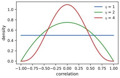
Filling the gap 3.14: the LKJ prior in two dimensions pp. 101–102, (3.216)–(3.217)
Derivation
For \(D=2\), \[R=\begin{pmatrix}1&\rho\\\rho&1\end{pmatrix}\], \(|R|=1-\rho^2\), and the free element is \(\rho\in(-1,1)\); so the LKJ density is \(p(\rho)\propto(1-\rho^2)^{\eta-1}\). Substituting \(\rho=2b-1\), \(1-\rho^2=4b(1-b)\), the density of \(b\) is \(\propto b^{\eta-1}(1-b)^{\eta-1}\): \(b\sim\Beta(\eta,\eta)\), and the normalised density of \(\rho\) is \((1-\rho^2)^{\eta-1}/(2^{2\eta-1}B(\eta,\eta))\). For \(\eta=1\) it is uniform with density \(\frac12\); for \(\eta=2\) it is \(\frac34(1-\rho^2)\), with \(\E\rho^2=\frac15\) (confirmed by rejection sampling). In general the prior is symmetric about 0, and for \(\eta>1\) pushes mass to \(\rho=0\), vanishing as \(|\rho|\to1\).
Cholesky form. With \(R=LL^\T\), \[L=\begin{pmatrix}1&0\\\rho&\sqrt{1-\rho^2}\end{pmatrix}\], the free entry is \(L_{21}=\rho\) with unit Jacobian, so the density in \(L\) is \((1-\rho^2)^{\eta-1}=L_{22}^{2\eta-2}\). In general the LKJ density on the Cholesky factor is \(\prod_{i=2}^DL_{ii}^{D-i+2\eta-2}\); the exponent \(-\eta-1\) printed in (3.217) does not reduce to this for \(D=2\) (it would give \(L_{22}^{-2}\) at \(\eta=1\), which is not uniform), so I treat (3.217) as a misprint. \(\square\)
3.5 Noninformative priors
pp. 102–107 With little domain knowledge one wants a prior that "lets the data speak". No prior is truly uninformative; the honest names are diffuse, minimally informative or default priors. Four constructions follow.
3.5.1 Maximum entropy priors
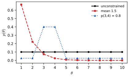
pp. 102–104 Pick the prior of largest entropy subject to constraints \(\E[f_k(\theta)]=F_k\) (Laplace's principle of insufficient reason when there are none). For a Bernoulli rate this is \(\Beta(1,1)\). For \(\theta\in\{1,\dots,10\}\) with mean 1.5 the solution is a decaying exponential; if \(\Pr(\theta\in\{3,4\})=0.8\) it is flat except for a plateau on 3 and 4 (3.218)–(3.220).
Filling the gap 3.15: maximum entropy distributions are exponential families, with a proof of global optimality pp. 102–104, Section 2.4.7
Derivation
Let \(\Theta\) be finite, \(H(p)=-\sum_cp_c\log p_c\), constraints \(\sum_cp_cf_k(c)=F_k\), \(k=1..K\). Claim: if there is \(\bm\lambda\) with \[p^*_c=Z(\bm\lambda)^{-1}\exp(\sum_k\lambda_kf_k(c))\] satisfying the constraints, \(Z=\sum_c\exp(\sum_k\lambda_kf_k(c))\), then \(p^*\) is the unique maximiser.
Proof. For any \(q\) satisfying the constraints, by Gibbs' inequality \[-\sum_cq_c\log q_c\le-\sum_cq_c\log p^*_c=-\sum_k\lambda_k\sum_cq_cf_k(c)+\log Z=-\bm\lambda^\T\bm F+\log Z\], with equality iff \(q=p^*\). The same computation for \(q=p^*\) shows \(H(p^*)=-\bm\lambda^\T\bm F+\log Z\), so \(H(q)\le H(p^*)\). (Lagrange multipliers would only give stationarity: the entropy is strictly concave, which the Gibbs argument uses implicitly.)
Mean constraint on \(\{1..10\}\). \(p_c\propto e^{\lambda c}\); the mean is strictly increasing in \(\lambda\) (its derivative is the variance), so \(\E c=1.5\) has a unique root, \(\lambda=-\log3\), i.e. \(p_c=\frac23\cdot3^{-(c-1)}\) up to the truncation at 10 (\(p_1=0.6666\), \(p_2=0.2223\)). Indicator constraint. \(f(c)=\mathbb 1[c\in\{3,4\}]\), \(p_c\propto e^{\lambda f(c)}\) is constant on \(\{3,4\}\) and on the other eight values; the constraint forces \(p_3=p_4=0.4\) and the rest \(0.2/8=0.025\), so \(e^\lambda=16\). Both were confirmed by constrained numerical optimisation. \(\square\)
3.5.2 Jeffreys priors
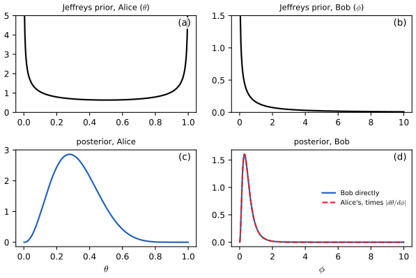
pp. 103–106 The posterior should not depend on how the model is parameterised. Alice parameterises a Bernoulli model by the rate \(\theta\), Bob by the odds \(\phi=\theta/(1-\theta)\); if Bob converts Alice's prior by the change-of-variables formula, he gets the same posterior as Alice. In 1-d the Jeffreys prior \(p(\theta)\propto\sqrt{F(\theta)}\), and in general \(p(\bm\theta)\propto\sqrt{\det F(\bm\theta)}\), has this property. For the binomial \(F=n/(\theta(1-\theta))\) gives \(\Beta(\frac12,\frac12)\) (3.225); in the odds, \(F(\phi)=\frac n{\phi(\phi+1)^2}\) and \(p(\phi)\propto\phi^{-1/2}(1+\phi)^{-1}\) (3.226)–(3.232); for a categorical variable \(\Dir(\frac12,\dots,\frac12)\) (3.233), not \(\Dir(\frac1K,\dots)\) or \(\Dir(1,\dots)\); for a Gaussian \((\mu,\sigma^2)\), see below.
Filling the gap 3.16: invariance of the Jeffreys prior in any dimension, and the binomial, multinomial and Gaussian cases pp. 103–106, (3.221)–(3.236)
Derivation
Invariance. Let \(\bm\theta=\bm\theta(\bm\phi)\) be a smooth invertible reparameterisation with Jacobian \(J=\partial\bm\theta/\partial\bm\phi\). Jeffreys' rule applied in the \(\bm\phi\)-parameterisation gives \[p_\phi(\bm\phi)\propto\sqrt{\det F_\phi(\bm\phi)}\], and by gap 3.6 \(F_\phi=J^\T F_\theta J\), so \[\sqrt{\det F_\phi}=|\det J|\sqrt{\det F_\theta}\]. On the other hand pushing the Jeffreys prior of \(\bm\theta\) through the change of variables gives the density \[p_\theta(\bm\theta(\bm\phi))\,|\det J|\propto\sqrt{\det F_\theta}\,|\det J|\]. The two coincide: applying the rule in either parameterisation yields the same measure on parameter space. (The book's one-dimensional chain (3.221)–(3.224) is this computation; the step "\[\E[(\d\log p/\d\theta\,\d\theta/\d\phi)^2]=\E[(\d\log p/\d\phi)^2]\]" is the chain rule for the score.) Consequently posteriors agree: \[p(\theta\given\mathcal D)\propto p(\mathcal D\given\theta)p_J(\theta)\] transforms like a density under any smooth reparameterisation. A flat prior has no such property, since uniform in \(\phi\) is \(|\d\phi/\d\theta|\) in \(\theta\); the demonstration Jeffreys priors and reparameterisation computes the Fisher information of the new parameterisation numerically from the likelihood to show this.
Binomial. \(F(\theta)=n/(\theta(1-\theta))\) gives \[p(\theta)\propto\theta^{-1/2}(1-\theta)^{-1/2}\], the \(\Beta(\frac12,\frac12)\) density (normaliser \(B(\frac12,\frac12)=\pi\)), and the posterior \(\Beta(x+\frac12,n-x+\frac12)\); for \(n=10,x=3\) its mean is \(3.5/11=0.318\), against \(0.333\) for the uniform prior. In the odds, with \(\theta=\phi/(1+\phi)\), \(\ell=x\log\phi-n\log(1+\phi)\), \(\ell''=-x/\phi^2+n/(1+\phi)^2\), and \(\E x=n\phi/(1+\phi)\) gives \[F(\phi)=\frac n{\phi(1+\phi)}-\frac n{(1+\phi)^2}=\frac n{\phi(1+\phi)^2}\] (3.230)–(3.231), hence \(p(\phi)\propto\phi^{-1/2}(1+\phi)^{-1}\) (3.232). Check: \(\phi^{-1/2}(1+\phi)^{-1}\) is the push-forward of \(\theta^{-1/2}(1-\theta)^{-1/2}\) times \(|\d\theta/\d\phi|=(1+\phi)^{-2}\): \[\big(\frac\phi{1+\phi}\big)^{-1/2}\big(\frac1{1+\phi}\big)^{-1/2}(1+\phi)^{-2}=\phi^{-1/2}(1+\phi)^{-1}\]. \(\checkmark\) In the arcsine parameterisation \(\varphi=2\arcsin\sqrt\theta\) the Fisher information is constant (\(F=n\)), so the Jeffreys prior is uniform in \(\varphi\): the variance-stabilising transform.
Multinomial. Use free coordinates \(\theta_1,\dots,\theta_{K-1}\), \(\theta_K=1-\sum_{i<K}\theta_i\). The log likelihood of one observation is \(\sum_{k\le K}\mathbb 1[x=k]\log\theta_k\), so \[F_{ij}=\E[\partial_i\ell\,\partial_j\ell]=\delta_{ij}/\theta_i+1/\theta_K\], i.e. \[F=\diag(1/\theta_i)+\theta_K^{-1}\bm 1\bm 1^\T\]. By the matrix determinant lemma \[\det F=\prod_{i<K}\theta_i^{-1}\,(1+\theta_K^{-1}\sum_{i<K}\theta_i)=\prod_{i<K}\theta_i^{-1}\cdot\theta_K^{-1}\]. So \[\sqrt{\det F}=\prod_{k=1}^K\theta_k^{-1/2}\propto\Dir(\frac12,\dots,\frac12)\] (3.233).
Gaussian. In the parameters \((\mu,v)\), \(v=\sigma^2\), \(F=\diag(1/v,1/(2v^2))\) (3.62), so \(\sqrt{\det F}=1/(\sqrt2\,v^{3/2})\); in the parameters \((\mu,\sigma)\) the same prior is \(\sqrt2/\sigma^2\) (multiply by \(|\d v/\d\sigma|=2\sigma\): \[\frac{1}{\sqrt2\sigma^3}2\sigma\propto\sigma^{-2}\]). The book's (3.234) is labelled with \(\theta=(\mu,\sigma)\) but is the information in \((\mu,v)\); the displayed \(\sqrt{\det}\) is correct for \((\mu,v)\). The joint Jeffreys prior is thus \(v^{-3/2}\), not the \(1/\sigma^2\) of (3.235); the latter is the Jeffreys recommendation of treating location and scale separately, \(p(\mu)p(\sigma^2)\propto1\cdot\sigma^{-2}\), each being the Jeffreys prior of its own parameter with the other fixed (\(F_{\mu\mu}\) constant, \(F_{\sigma\sigma}\propto\sigma^{-2}\), so \(p(\sigma)\propto1/\sigma\), i.e. \(p(\sigma^2)\propto1/\sigma^2\)). It is the \(\NIX(0,0,-1,0)\) prior of gap 3.9. \(\square\)
3.5.3 Invariant priors
pp. 106–107 Invariances can be built into the prior directly. A translation-invariant prior on a location satisfies \(\int_{A-c}^{B-c}p=\int_A^Bp\) for all \(c\), which holds for \(p(\mu)\propto1\) (3.237)–(3.239) (and only for it, up to a constant, since a measure invariant under all shifts of \(\mathbb R\) is Lebesgue measure); this equals the Jeffreys prior of the Gaussian mean because \(F(\mu)=1/\sigma^2\) is constant. A scale-invariant prior satisfies \(\int_{A/c}^{B/c}p=\int_A^Bp\) for all \(c>0\), which holds for \(p(\sigma)\propto1/\sigma\) (3.240)–(3.242), since \(\int_{A/c}^{B/c}\d\sigma/\sigma=\log B-\log A\) (equivalently, flat in \(\log\sigma\), which is translation invariant in \(\log\sigma\)); it equals the Jeffreys prior \(\sqrt{F(\sigma)}=\sqrt2/\sigma\). Both are improper. When an invariance has no closed form the prior can be learned by optimisation (Section 3.5.3.3, Nalisnick and Smyth, 2018).
3.5.4 Reference priors
p. 107 A reference prior maximises the expected KL divergence from posterior to prior, i.e. the mutual information between parameter and data, \[p^*=\argmax_p\int p(\mathcal D)\KL(p(\theta\given\mathcal D)\|p(\theta))\,\d\mathcal D=\argmax_pI(\theta;\mathcal D)\] (3.243), which equals \[\E_\theta[\KL(p(\mathcal D\given\theta)\|p(\mathcal D))]\] (3.244); in one dimension the maximiser is, for large \(N\), the Jeffreys prior.
Filling the gap 3.17: the identity (3.244) and why the reference prior is Jeffreys' prior asymptotically p. 107, (3.243)–(3.244)
Derivation
The identity. \[\int p(\mathcal D)\int p(\theta\given\mathcal D)\log\frac{p(\theta\given\mathcal D)}{p(\theta)}\,\d\theta\,\d\mathcal D=\iint p(\theta,\mathcal D)\log\frac{p(\theta,\mathcal D)}{p(\theta)p(\mathcal D)}\], the mutual information \(I(\theta;\mathcal D)\). Swapping the order of integration and using \[\frac{p(\theta\given\mathcal D)}{p(\theta)}=\frac{p(\mathcal D\given\theta)}{p(\mathcal D)}\] turns it into \[\int p(\theta)\int p(\mathcal D\given\theta)\log\frac{p(\mathcal D\given\theta)}{p(\mathcal D)}=\E_\theta\KL(p(\mathcal D\given\theta)\|p(\mathcal D))\] (3.244).
Asymptotics (heuristic under regularity, Clarke and Barron, 1994). For \(\mathcal D\) of size \(N\) and a smooth prior, the posterior is approximately \(\mathcal N(\hat\theta,(NF(\hat\theta))^{-1})\) (Bernstein–von Mises). Write \[I=\E\log p(\theta\given\mathcal D)-\E\log p(\theta)\] (the entropy form of mutual information). Under this normal approximation \[\E\log p(\theta\given\mathcal D)\approx\E_\theta[\frac12\log\det(NF(\theta)/2\pi)-\frac d2]\], so \[ I(\theta;\mathcal D_N)=\frac d2\log\frac N{2\pi e}+\int p(\theta)\log\frac{\sqrt{\det F(\theta)}}{p(\theta)}\,\d\theta+o(1). \] With \(Z_J=\int\sqrt{\det F}\) and \(p_J=\sqrt{\det F}/Z_J\) the last integral is \(\log Z_J-\KL(p\|p_J)\le\log Z_J\), with equality iff \(p=p_J\). Hence the mutual information is maximised, to leading order, by the Jeffreys prior, which is the one-parameter reference prior (3.243). For the binomial \(Z_J=\pi\), and the uniform prior loses \(\KL(\mathrm{Unif}\|p_J)=\log\pi-1=0.145\) nats; at \(N=150\) the exact mutual informations (computed by summation) are 2.274 for \(\Beta(\frac12,\frac12)\), 2.098 for \(\Beta(1,1)\) and 1.809 for \(\Beta(2,2)\), the same order. In higher dimensions the reference prior is built one parameter at a time and can differ from Jeffreys' (Bernardo, 1979). \(\square\)
3.6 Hierarchical priors
pp. 108–114 If the hyperparameters \(\xi\) of the prior are unknown, put a prior on them: \[p(\xi,\theta,\mathcal D)=p(\xi)p(\theta\given\xi)p(\mathcal D\given\theta)\] (3.245). With \(J\) related datasets with parameters \(\theta_j\), the model borrows statistical strength: groups with little data are pulled towards the population. Predictions for an existing group use \[\int p(y_j\given\theta_j)p(\theta_j\given\mathcal D)\,\d\theta_j\] (3.246), for a new group \[\int p(y_*\given\theta_*)p(\theta_*\given\xi)p(\xi\given\mathcal D)\,\d\theta_*\d\xi\] (3.247).
3.6.1 A hierarchical binomial model
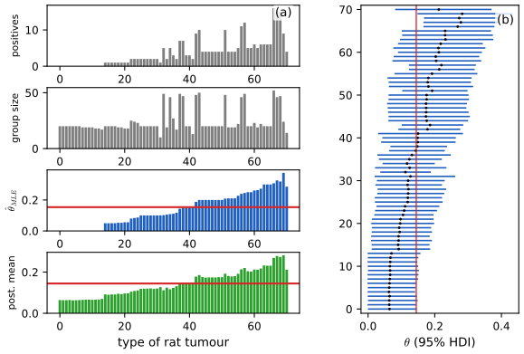
pp. 108–111 Group \(j\) has \(N_j\) animals and \(y_j\) positives, \(y_j\sim\Bin(N_j,\theta_j)\), \(\theta_j\sim\Beta(a,b)\); no pooling uses \(\hat\theta_j=y_j/N_j\), complete pooling \(\hat\theta=\sum y_j/\sum N_j\). The joint is (3.248) with the prior \(p(a,b)\propto(a+b)^{-5/2}\) (3.249). The book samples the unconstrained \(\omega=(\tilde\theta,\tilde\xi)\) by HMC with log Jacobians of the sigmoid and softplus transforms (3.250)–(3.251); I use an exact computation instead (gap 3.18). For the 71-group rat tumour data, groups with \(y_j=0\) are pulled up to about 0.06 and large groups barely move: shrinkage.
Filling the gap 3.18: the posterior of the hierarchical binomial model without MCMC pp. 108–111, (3.248)–(3.251)
Derivation
Integrating out the group rates. Given \((a,b)\) the groups are independent and each \(\theta_j\) is conjugate: \[\int\Bin(y_j\given N_j,\theta_j)\Beta(\theta_j\given a,b)\,\d\theta_j=\binom{N_j}{y_j}\frac{B(a+y_j,b+N_j-y_j)}{B(a,b)}\] (3.261)–(3.263). Therefore \[ p(a,b\given\mathcal D)\propto p(a,b)\prod_{j=1}^J\frac{B(a+y_j,b+N_j-y_j)}{B(a,b)}, \] a two-dimensional density that can be evaluated on a grid; and given \((a,b)\), \[\theta_j\given a,b,\mathcal D\sim\Beta(a+y_j,b+N_j-y_j)\] independently. So exact posterior samples are: draw \((a,b)\) from the grid, then draw each \(\theta_j\) from its beta. The grid is laid on \((u,v)=(\log\frac ab,\log(a+b))\) where the posterior is smooth; the Jacobian of \((a,b)\mapsto(u,v)\) is \(ab\) (with \(a=e^v\sigma(u)\), \(b=e^v(1-\sigma(u))\): \(\det=e^{2v}\sigma(u)(1-\sigma(u))=ab\)), so the density on the grid is \(p(a,b\given\mathcal D)\,ab\). This is the same change-of-variables bookkeeping as the Jacobian terms of (3.250)–(3.251): omitting it would sample a different distribution.
The prior is uniform in interpretable coordinates. Let \(m=a/(a+b)\) (prior mean) and \(s=(a+b)^{-1/2}\). Then \(a=ms^{-2}\), \(b=(1-m)s^{-2}\) and \(|\partial(a,b)/\partial(m,s)|=2s^{-5}\) (compute: \[\det\begin{pmatrix}s^{-2}&-2ms^{-3}\\-s^{-2}&-2(1-m)s^{-3}\end{pmatrix}=-2s^{-5}\]). Since \((a+b)^{-5/2}=s^5\), \(p(a,b)\,\d a\,\d b=2\,\d m\,\d s\): the book's prior (3.249) is flat in the prior mean and in \((a+b)^{-1/2}\), a weakly informative choice that is proper on bounded ranges.
Result. The posterior mean of \(a/(a+b)\) is 0.145 (the pooled MLE is 0.154), \(\E[a]=2.42\), \(\E[b]=14.4\). Each group's posterior mean is \(\E\big[\frac{a+y_j}{a+b+N_j}\big]\), a shrinkage estimate with data-dependent weight \(N_j/(N_j+a+b)\). A fine-grid run (\(400^2\) against \(260^2\) cells) gave the same means to within 0.005 in the population mean. \(\square\)
3.6.2 A hierarchical Gaussian model
pp. 111–114 With \(N_j\) observations \(y_{ij}\sim\mathcal N(\theta_j,\sigma^2)\), the group mean \(y_j=\frac1{N_j}\sum_iy_{ij}\) is a single observation of variance \(\sigma_j^2=\sigma^2/N_j\), so the model is \(y_j\sim\mathcal N(\theta_j,\sigma_j^2)\), \(\theta_j\sim\mathcal N(\mu,\tau^2)\) (3.252). In the eight schools problem (Gelman et al., 2014, Section 5.5; the effect of a coaching programme on SAT scores) school 0 has an unusually large improvement, 28 points; the pooled estimate is the precision-weighted mean \[y_{\cdot\cdot}=\sum_jy_j/\sigma_j^2\big/\sum_j1/\sigma_j^2\] (3.253), here 7.69. The posterior means of the \(\theta_j\) are shrunk towards \(\mu\): with hyperparameters fixed at their posterior means, \[\E[\theta_j\given\mathcal D,\mu,\tau^2]=w_j\mu+(1-w_j)y_j\], \(w_j=\sigma_j^2/(\sigma_j^2+\tau^2)\) (3.256)–(3.257): more shrinkage for noisier groups and for smaller \(\tau\).
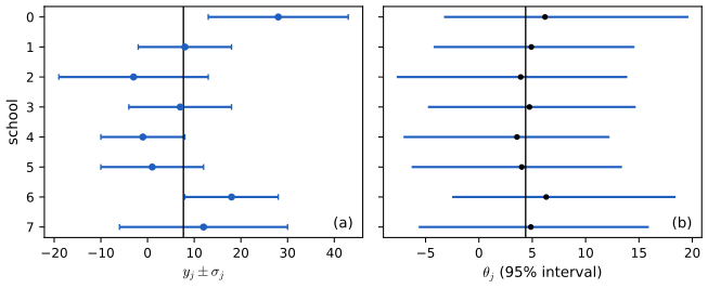
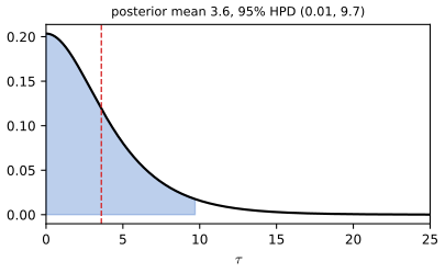
Filling the gap 3.19: the exact posterior of the eight-schools model, \(p(\tau\given\mathcal D)\) and the shrinkage weights pp. 111–112, (3.252)–(3.257)
Derivation
Marginal over \(\theta\). Given \((\mu,\tau)\) the school effects are independent, and \[\int\mathcal N(y_j\given\theta_j,\sigma_j^2)\mathcal N(\theta_j\given\mu,\tau^2)\,\d\theta_j=\mathcal N(y_j\given\mu,\sigma_j^2+\tau^2)\] (the same convolution as (3.264)).
Marginal over \(\mu\). Let \(d_j=\sigma_j^2+\tau^2\), \(w_j=1/d_j\). With \(\mu\sim\mathcal N(m_0,s_0^2)\), completing the square in \(\mu\) gives the posterior \[\mu\given\tau,\bm y\sim\mathcal N(\bar\mu_\tau,V_\tau)\] with \(V_\tau^{-1}=\sum_jw_j+s_0^{-2}\), \(\bar\mu_\tau=V_\tau(\sum_jw_jy_j+m_0s_0^{-2})\), and \[ p(\bm y\given\tau)=\prod_j(2\pi d_j)^{-1/2}\ (s_0^2V_\tau^{-1})^{-1/2}\ \exp\Big\{-\tfrac12\sum_jw_jy_j^2-\tfrac{m_0^2}{2s_0^2}+\tfrac{(\sum_jw_jy_j+m_0s_0^{-2})^2}{2V_\tau^{-1}}\Big\}. \] (For a flat prior on \(\mu\), drop \(s_0\): \[\prod_jd_j^{-1/2}(\sum w_j)^{-1/2}\exp(-\frac12\sum_jw_j(y_j-\hat\mu_\tau)^2)\], \(\hat\mu_\tau=\sum w_jy_j/\sum w_j\).) Then \[p(\tau\given\bm y)\propto p(\tau)p(\bm y\given\tau)\], a one-dimensional density evaluated on a grid; with \(\tau\sim\) half-Cauchy(5), \(\mu\sim\mathcal N(0,5^2)\) it has mean 3.60, in agreement with the book's 3.6. A flat prior on \(\tau\) would give a larger \(\E\tau\approx6.5\), showing the dependence on this prior.
School effects. Given \((\mu,\tau)\), \(\theta_j\) is a Gaussian conjugate update: precision \(\sigma_j^{-2}+\tau^{-2}\), mean \[\frac{y_j/\sigma_j^2+\mu/\tau^2}{\sigma_j^{-2}+\tau^{-2}}=(1-w_j)y_j+w_j\mu\] with \(w_j=\frac{\sigma_j^2}{\sigma_j^2+\tau^2}\) (multiply numerator and denominator by \(\sigma_j^2\tau^2\)), and variance \((1-w_j)\sigma_j^2\) (3.256)–(3.257). Since the mean is linear in \(\mu\), \[\E[\theta_j\given\tau,\bm y]=(1-w_j)y_j+w_j\bar\mu_\tau\] and, averaging over \(\tau\), \[\E[\theta_j\given\mathcal D]=\int\{(1-w_j(\tau))y_j+w_j(\tau)\bar\mu_\tau\}p(\tau\given\bm y)\,\d\tau\]: a quadrature that the demonstration performs. Exact sampling draws \(\tau\) from its grid, then \(\mu\), then each \(\theta_j\). Fixing \((\mu,\tau)\) at their means (3.254)–(3.255) gives only an approximation: it ignores the spread of \(p(\tau\given\mathcal D)\), which is wide (the HPD runs from near 0 to about 10). \(\square\)
3.6.2.2 Non-centered parameterization
pp. 112–114 Posterior inference by local-move algorithms is hard because \(\tau\) and the \(\theta_j\) are strongly dependent: the funnel of Figure 3.18a. The non-centred form \(\theta_j=\mu+\tau\eta_j\), \(\eta_j\sim\mathcal N(0,1)\) (3.258)–(3.259) makes \(\eta\) a priori independent of \((\mu,\tau)\) (Figure 3.19b).
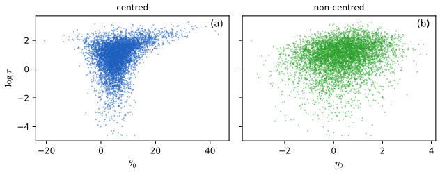
Filling the gap 3.20: why the centred funnel defeats local samplers and the non-centred form does not pp. 112–114
Argument and a numerical test
Geometry. In the centred form the prior of the effects is \(\prod_j\mathcal N(\theta_j\given\mu,\tau^2)\), so \(-\log p\) contains \[\frac1{2\tau^2}\sum_j(\theta_j-\mu)^2+J\log\tau\]. The curvature in each \(\theta_j\) is \(1/\tau^2\) (plus \(1/\sigma_j^2\) from the likelihood). Across the funnel \(\tau\) ranges over orders of magnitude, so the curvature, hence the scale on which a gradient-based or random-walk proposal must move, varies by factors \(\tau^{-2}\): a step size small enough for the neck (\(\tau\) small, all \(\theta_j\) within \(\tau\) of \(\mu\)) makes exploration of the mouth hopelessly slow, and a step size adequate for the mouth overshoots in the neck, where the integrator diverges. The neck can only be entered when all \(\theta_j\) move towards \(\mu\) together.
Non-centred form. With \(\theta_j=\mu+\tau\eta_j\) the prior part of the target is \(\prod_j\mathcal N(\eta_j\given0,1)\), independent of \((\mu,\tau)\); the dependence on \(\tau\) enters only through the likelihood \[\mathcal N(y_j\given\mu+\tau\eta_j,\sigma_j^2)\], whose curvature in \(\eta_j\) is \(\tau^2/\sigma_j^2\), bounded when \(\tau\lesssim\sigma_j\), which is the regime of weak data (as here). When the data are very informative (\(\sigma_j\ll\tau\)) the centred form is the better one (Betancourt and Girolami, 2015).
Numerical test. I implemented Hamiltonian Monte Carlo (step size 0.05, 30 leapfrog steps, 6000 iterations, analytic gradients, \(\log\tau\) as the unconstrained variable with its log-Jacobian) for both forms. Non-centred: 0 divergent transitions, effective sample size of \(\log\tau\) about 1470, posterior mean of \(\tau\) 3.56 against the exact 3.60. Centred: 30 divergent transitions and an effective sample size of about 70, the same posterior but far less efficiently. Both forms target the same distribution; only the coordinates differ. \(\square\)
3.7 Empirical Bayes
pp. 114–118 Full hierarchical inference can be costly. Empirical Bayes (EB) picks the hyperparameters by maximising the marginal likelihood, \[\hat\xi=\argmax_\xi\int p(\mathcal D\given\theta)p(\theta\given\xi)\,\d\theta\] (3.260) (type II maximum likelihood, the evidence procedure), then uses \(p(\theta\given\hat\xi,\mathcal D)\). It violates the rule that priors are chosen independently of the data, but is a cheap approximation to the full hierarchical posterior, and less prone to overfit than ML because there are few hyperparameters. The book's ladder: ML \(\hat\theta=\argmax p(\mathcal D\given\theta)\); MAP \[\argmax p(\mathcal D\given\theta)p(\theta\given\xi)\]; ML-II \[\hat\xi=\argmax_\xi\int p(\mathcal D\given\theta)p(\theta\given\xi)\d\theta\]; MAP-II adds \(p(\xi)\); full Bayes \(p(\theta,\xi\given\mathcal D)\): the more integrals, the more Bayesian.
3.7.1 EB for the hierarchical binomial model
p. 115 The \(\theta_j\) integrate out analytically, so \[p(\mathcal D\given a,b)\propto\prod_jB(a+y_j,b+N_j-y_j)/B(a,b)\] (3.261)–(3.263); maximising over \((a,b)\) (Minka, 2000, gives fixed-point iterations; here a derivative-free search on \((\log a,\log b)\)) yields \(\hat a=2.34\), \(\hat b=14.11\) with \(\log p=-730.34\) on the rat data, prior mean \(0.142\). The posterior means \((\hat a+y_j)/(\hat a+\hat b+N_j)\) differ from the full Bayesian ones by at most 0.004.
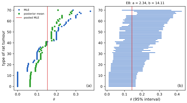
3.7.2 EB for the hierarchical Gaussian model
p. 116 With equal variances \(\sigma_j^2=\sigma^2\), marginally \(y_j\sim\mathcal N(\mu,\tau^2+\sigma^2)\) (3.264)–(3.265), so \(\hat\mu=\bar y\) (3.266), and \(\hat\tau^2=\max\{0,v-\sigma^2\}\) with \(v=\frac1J\sum_j(y_j-\bar y)^2\) (3.267)–(3.268); the estimate is \(\hat\theta_j=\lambda\hat\mu+(1-\lambda)y_j\), \(\lambda=\sigma^2/(\sigma^2+\hat\tau^2)\) (3.269). Unequal variances (eight schools) need EM or numerical optimisation.
Filling the gap 3.21: the EB estimate for the equal-variance Gaussian hierarchy, including the positive part p. 116, (3.264)–(3.269)
Derivation
The log marginal likelihood is \[\ell(\mu,s)=-\frac J2\log(2\pi s)-\frac1{2s}\sum_j(y_j-\mu)^2\] with \(s=\tau^2+\sigma^2\ge\sigma^2\). For fixed \(s\) it is maximised at \(\mu=\bar y\) (a concave quadratic), leaving \(\ell(s)=-\frac J2(\log s+v/s)+\mathrm{const}\), \(v=\frac1J\sum(y_j-\bar y)^2\). Its derivative \[-\frac J2(\frac1s-\frac v{s^2})=\frac J{2s^2}(v-s)\] is positive for \(s<v\) and negative for \(s>v\): \(\ell\) is unimodal with maximum at \(s=v\) (the book's "moment matching" is the same as ML for a Gaussian). On the constraint set \(s\ge\sigma^2\): if \(v\ge\sigma^2\) the maximiser is \(s=v\), \(\hat\tau^2=v-\sigma^2\); if \(v<\sigma^2\), \(\ell\) is decreasing on \([\sigma^2,\infty)\) and the constrained maximum is at the boundary, \(\hat\tau^2=0\): total pooling. Hence \(\hat\tau^2=(v-\sigma^2)_+\) (3.268). Both cases were confirmed by numerical optimisation. The posterior mean given \(\hat\mu,\hat\tau^2\) is \[\frac{y_j/\sigma^2+\hat\mu/\hat\tau^2}{\sigma^{-2}+\hat\tau^{-2}}=\lambda\hat\mu+(1-\lambda)y_j\], \(\lambda=\frac{\sigma^2}{\sigma^2+\hat\tau^2}\) (3.269), which is \(\hat\mu\) for \(\hat\tau^2=0\).
A caution. The plug-in posterior treats \((\hat\mu,\hat\tau^2)\) as known, so its intervals are too narrow compared with full Bayes (they ignore the width of \(p(\tau\given\mathcal D)\)): for the eight schools the marginal likelihood \(p(\bm y\given\tau)\) (flat prior on \(\mu\)) is largest at \(\tau=0\), so ML-II would pool completely, whereas the full posterior of \(\tau\) spreads over \((0,10)\) (checked on a grid). \(\square\)
3.7.3 EB for Markov models (n-gram smoothing)
pp. 116–118 Deleted interpolation estimates the transition matrix as \(A_{jk}=(1-\lambda)f_{jk}+\lambda f_k\) with bigram frequencies \(f_{jk}=N_{jk}/N_j\) and unigram frequencies \(f_k=N_k/N\) (3.270), \(\lambda\) set by cross validation. The Bayesian version puts \(A_j\sim\Dir(\alpha_0\bm m)\) on every row with shared hyperparameters (Figure 3.21), giving the predictive \[p(X_{t+1}=k\given X_t=j,\mathcal D)=(1-\lambda_j)f_{jk}+\lambda_jm_k\], \(\lambda_j=\alpha_0/(N_j+\alpha_0)\) (3.272)–(3.274): a context-dependent weight, backing off to \(m_k\) rather than \(f_k\). The hyperparameters follow from \[p(\mathcal D\given\bm\alpha)=\prod_jB(\bm N_j+\bm\alpha)/B(\bm\alpha)\] (3.275), approximately \(m_k\propto|\{j:N_{jk}>0\}|\) (3.276) (MacKay and Peto, 1995).
Filling the gap 3.22: the n-gram predictive as shrinkage towards the prior mean, and the number-of-contexts heuristic pp. 116–118, (3.270)–(3.276)
Derivation
Predictive. The posterior of row \(j\) is \(\Dir(\bm\alpha+\bm N_j)\) with \(\bm\alpha=\alpha_0\bm m\), \(\sum_km_k=1\). Its mean is \((N_{jk}+\alpha_0m_k)/(N_j+\alpha_0)\), and the predictive probability of the next state equals the posterior mean (gap 3.1). Writing \(N_{jk}=N_jf_{jk}\): \[\frac{N_j}{N_j+\alpha_0}f_{jk}+\frac{\alpha_0}{N_j+\alpha_0}m_k=(1-\lambda_j)f_{jk}+\lambda_jm_k\] (3.272)–(3.274). Compared with (3.270): the weight on the backoff shrinks as the context \(j\) is seen more often (\(\lambda_j\to0\) as \(N_j\to\infty\)), the prior being worth \(\alpha_0\) pseudo-observations, and the backoff target is the prior mean \(\bm m\) instead of the corpus frequency \(f_k\).
Why contexts, not counts. Put \(x_k=\alpha_0m_k\). The row-\(j\) factor of (3.275) contains \(\prod_k\Gamma(N_{jk}+x_k)/\Gamma(x_k)\). For \(N_{jk}=0\) this factor is 1. For \(N_{jk}\ge1\) and small \(x_k\), \[\Gamma(n+x)/\Gamma(x)=x\,\Gamma(n+x)/\Gamma(1+x)\to x\,\Gamma(n)\] as \(x\to0\) (use \(\Gamma(x)=\Gamma(1+x)/x\)). So for sparse data, where the optimal \(x_k\) are small, \[\log p(\mathcal D\given\bm\alpha)\approx\sum_kc_k\log x_k+(\text{terms not depending on }\bm m)\], where \(c_k=|\{j:N_{jk}>0\}|\) is the number of contexts in which word \(k\) occurs; the denominator terms \(\Gamma(\alpha_0)/\Gamma(N_j+\alpha_0)\) do not involve \(\bm m\). Maximising \(\sum_kc_k\log m_k\) subject to \(\sum_km_k=1\) (Gibbs' inequality, as in gap 3.15) gives \(m_k=c_k/\sum_{k'}c_{k'}\propto c_k\) (3.276). It is an approximation, exact only in the small-\(x\) limit (MacKay and Peto, 1995). In a numerical experiment with 30 contexts, a word following 29 different contexts once each (38 occurrences) received the maximum likelihood value \(m=0.30\) while a word appearing 47 times but after a single context received \(m=0.04\), in line with the "you see" example of the book. \(\square\)
p. 118 The Bayesian model does not beat interpolated Kneser–Ney, which a hierarchical Pitman–Yor construction recovers, nor recurrent networks that share strength through embeddings. For non-conjugate models EB uses variational EM (Section 10.1.3.2).
S3.3 Tweedie's formula: empirical Bayes without estimating the prior (supplement)
Supplement pp. 36–37 Tweedie's formula (Efron, 2011) estimates a latent quantity from noisy observations without modelling the prior: it replaces the prior by an estimate of the score of the marginal density of the observation. Let the natural parameter \(\eta\) have a prior \(g(\eta)\) and \[y\given\eta\sim f_\eta(y)=e^{\eta y-\psi(\eta)}f_0(y)\] (S3.23), with cumulant generating function \(\psi\) and base density \(f_0\) (for a Gaussian with variance \(\sigma^2\): \(\eta=\mu/\sigma^2\), \(\psi=\sigma^2\eta^2/2\), \(f_0=\mathcal N(0,\sigma^2)\)). With the marginal \(f(y)=\int f_\eta(y)g(\eta)\,\d\eta\) the posterior is itself an exponential family in \(y\), \[g(\eta\given y)=e^{y\eta-\lambda(y)}[g(\eta)e^{-\psi(\eta)}]\], \(\lambda(y)=\log\frac{f(y)}{f_0(y)}\) (S3.24)–(S3.27). The moments follow: \(\E[\eta\given y]=\ell'(y)-\ell_0'(y)\), \(\var[\eta\given y]=\ell''(y)-\ell_0''(y)\), \(\ell=\log f\), \(\ell_0=\log f_0\) (S3.29), and for the Gaussian \[ \E[\mu\given y]=y+\sigma^2\ell'(y),\qquad\var[\mu\given y]=\sigma^2\big(1+\sigma^2\ell''(y)\big) \tag{S3.30} \] and, for \(y\sim\mathcal N(\bm\mu,\Sigma)\) with vector \(\bm\mu\), \[\E[\bm\mu\given\bm y]=\bm y+\Sigma\nabla_{\bm y}\log p(\bm y)\] (S3.37). Plugging an estimate of the score \(\ell'\) (a kernel estimate, or for images a neural network, Section 24.3) gives an empirical Bayes estimate of the posterior mean without ever estimating the prior.
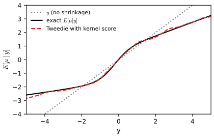
Filling the gap 3.39: Tweedie's formula in the exponential family and for the multivariate Gaussian Supplement pp. 36–37, (S3.23)–(S3.37)
Derivation
Posterior. By Bayes' rule \[g(\eta\given y)=\frac{f_\eta(y)g(\eta)}{f(y)}=\frac{e^{\eta y-\psi(\eta)}f_0(y)g(\eta)}{f(y)}=e^{y\eta-\lambda(y)}\,g(\eta)e^{-\psi(\eta)}\] with \(\lambda(y)=\log\frac{f(y)}{f_0(y)}\) (S3.26)–(S3.27). (The supplement writes the last factor as \(g(\eta)e^{-\psi(y)}\); it must be \(e^{-\psi(\eta)}\), as the line above it shows.) Since this is normalised for every \(y\), \[\lambda(y)=\log\int e^{y\eta}[g(\eta)e^{-\psi(\eta)}]\,\d\eta\] is the cumulant generating function of the measure \(g(\eta)e^{-\psi(\eta)}\,\d\eta\) in the variable \(y\) (up to normalisation).
Moments. Differentiating a cumulant generating function gives the mean and variance of the tilted distribution (as in gap 3.7): \[\E[\eta\given y]=\lambda'(y)=\ell'(y)-\ell_0'(y)\], \[\var[\eta\given y]=\lambda''(y)=\ell''(y)-\ell_0''(y)\] (S3.29). Gaussian: \(\ell_0(y)=-y^2/(2\sigma^2)+\mathrm{const}\), so \(\ell_0'=-y/\sigma^2\), \(\ell_0''=-1/\sigma^2\); with \(\eta=\mu/\sigma^2\): \[\E[\mu\given y]=\sigma^2\E[\eta\given y]=\sigma^2(\ell'+y/\sigma^2)=y+\sigma^2\ell'(y)\] and \[\var[\mu\given y]=\sigma^4(\ell''+1/\sigma^2)=\sigma^2(1+\sigma^2\ell'')\] (S3.30). Interpretation: the correction to \(y\) is the score of the marginal, pointing towards regions of high marginal density.
Multivariate. \[\nabla_yp(y\given\bm\mu)=p(y\given\bm\mu)\Sigma^{-1}(\bm\mu-\bm y)\] for \(\mathcal N(\bm y\given\bm\mu,\Sigma)\). Hence \[\frac{\nabla_yp(\bm y)}{p(\bm y)}=\frac{\int p(\bm\mu)\nabla_yp(\bm y\given\bm\mu)\,\d\bm\mu}{p(\bm y)}=\Sigma^{-1}\int p(\bm\mu\given\bm y)(\bm\mu-\bm y)\,\d\bm\mu=\Sigma^{-1}(\E[\bm\mu\given\bm y]-\bm y)\] (S3.33)–(S3.36), i.e. \[\E[\bm\mu\given\bm y]=\bm y+\Sigma\nabla_{\bm y}\log p(\bm y)\] (S3.37). Checks. For a Gaussian prior \(\mathcal N(\bm m_0,P_0)\) the marginal is \(\mathcal N(\bm m_0,P_0+\Sigma)\), the score is \(-(P_0+\Sigma)^{-1}(\bm y-\bm m_0)\), and \[\bm y+\Sigma\cdot\mathrm{score}=\bm m_0+P_0(P_0+\Sigma)^{-1}(\bm y-\bm m_0)\], the usual conjugate update; for a two-component Gaussian mixture prior both the mean and variance formulas (S3.30) agree with direct computation to \(10^{-6}\). \(\square\)
3.8 Model selection
pp. 118–128 Given a set \(\mathcal M\) of models, choose one or average over them. The M-complete assumption says the true model is in \(\mathcal M\); otherwise (M-open) no model is adequate and one must expand \(\mathcal M\), using the checks of Section 3.9.
3.8.1 Bayesian model selection
pp. 119–120 Pick \(\hat m=\argmax_mp(m\given\mathcal D)\), \[p(m\given\mathcal D)=\frac{p(\mathcal D\given m)p(m)}{\sum_{m'}p(\mathcal D\given m')p(m')}\] (3.277)–(3.278), which for a uniform prior is the model with the largest evidence \[p(\mathcal D\given m)=\int p(\mathcal D\given\theta,m)p(\theta\given m)\,\d\theta\] (3.279)–(3.280). A flexible model spreads prior mass over many parameter values that fit the data poorly, so it assigns lower density to any one dataset: the Bayesian Occam's razor.
Example: is the coin fair? \(M_0:\theta=\frac12\) has \(p(\mathcal D\given M_0)=2^{-N}\) (3.281); \(M_1\) (uniform or beta prior) has \[p(\mathcal D\given M_1)=B(\alpha_1+N_1,\alpha_0+N_0)/B(\alpha_1,\alpha_0)\] (3.282). For a sequence of \(N=5\) tosses and a uniform prior, \[\log_{10}p(\mathcal D\given M_1)=-0.78,-1.48,-1.78,-1.78,-1.48,-0.78\] for \(N_1=0,\dots,5\), against \(\log_{10}2^{-5}=-1.51\) for \(M_0\): the fair coin wins only for 2 or 3 heads (it would be a suspicious coincidence for a biased coin to give almost exactly half heads).
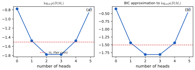
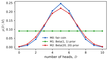
Filling the gap 3.23: probability conservation behind the Occam's razor, and the coin Bayes factor pp. 119–120, (3.280)–(3.282)
Derivation
Conservation. For every model \[\sum_{\mathcal D}p(\mathcal D\given m)=\sum_{\mathcal D}\int p(\mathcal D\given\theta,m)p(\theta\given m)\,\d\theta=\int p(\theta\given m)\cdot1\,\d\theta=1\] (sums over all possible datasets of the same size). A model can therefore only increase the evidence of some datasets by decreasing it for others. A simple model (few parameters, or a tight prior) concentrates its mass on a small set of datasets and gives them high evidence if they occur; a flexible model spreads it thin. The "waste" is quantified by the Laplace calculation of gap 3.27: \[\log p(\mathcal D\given m)\approx\log p(\mathcal D\given\hat\theta)-\log\frac{\text{prior volume}}{\text{posterior volume}}\], the log of the Occam factor.
Coin. For a specific sequence, \[p(\mathcal D\given M_1)=\int\theta^{N_1}(1-\theta)^{N_0}\,\d\theta=B(N_1+1,N_0+1)=\frac{N_1!N_0!}{(N+1)!}\], which for \(N=5\) is \[\frac16,\frac1{30},\frac1{60},\frac1{60},\frac1{30},\frac16\] for \(N_1=0..5\); the fair coin gives \(\frac1{32}\). The Bayes factor \(B_{1,0}=\frac{32}{6}=5.3\) for \(N_1=0\) (moderate to strong evidence for bias by Table 3.1) and \(\frac{32}{60}=0.53\) for \(N_1=2\) (weak evidence for the fair coin). For the binomial count instead of the sequence the factor \(\binom N{N_1}\) multiplies both models and cancels from \(B_{1,0}\). \(\square\)
3.8.2 Bayes model averaging
p. 121 For prediction, average over models: \[p(y\given\mathcal D)=\sum_mp(y\given m)p(m\given\mathcal D)\] (3.283) (Bayes model averaging, BMA). It resembles an ensemble but the weights sum to one, and if one model is best, \(p(m\given\mathcal D)\to1\) for it in the large-sample limit, unlike ensemble weights. A numerical example: with data from \(\mathcal N(0.3,1)\), \(M_0:\mu=0\) against \(M_1:\mu\sim\mathcal N(0,4)\), the average posterior weight of \(M_1\) is below 0.9 for \(N=10\) and above 0.9 for \(N=400\).
3.8.3 Estimating the marginal likelihood
pp. 121–122 (1) Analytic, for conjugate models (Section 3.4.5.4). (2) The harmonic mean estimator \[p(\mathcal D)\approx\big(\frac1S\sum_s1/p(\mathcal D\given\theta_s)\big)^{-1}\], \(\theta_s\sim p(\theta\given\mathcal D)\) (3.284) (the book's text writes \(\theta_s\sim p(\theta)\); the samples must come from the posterior). (3) Annealed importance sampling, sequential Monte Carlo, nested sampling. (4) Variational Bayes: the evidence lower bound \(\mathcal L(q)\le\log p(\mathcal D)\) (the book's "\(\log q(\mathcal D\given\theta)\)" is a garbled rendering of this bound).
Filling the gap 3.24: why the harmonic mean estimator is unbiased for \(1/p(\mathcal D)\) and yet unusable p. 121, (3.284)–(3.287)
Derivation
The identity. \[\E_{p(\theta\given\mathcal D)}\big[\frac1{p(\mathcal D\given\theta)}\big]=\int\frac1{p(\mathcal D\given\theta)}\frac{p(\mathcal D\given\theta)p(\theta)}{p(\mathcal D)}\,\d\theta=\frac1{p(\mathcal D)}\int p(\theta)\,\d\theta=\frac1{p(\mathcal D)}\] (3.285)–(3.287). So the sample average of \(1/L(\theta_s)\) is an unbiased estimate of \(1/p(\mathcal D)\) and the harmonic mean a consistent estimate of \(p(\mathcal D)\).
Infinite variance. The second moment is \[\E_{\rm post}[L^{-2}]=\frac1{p(\mathcal D)}\int\frac{p(\theta)}{L(\theta)}\,\d\theta\]. Take a Gaussian location model with likelihood \[L(\theta)\propto e^{-N(\theta-\bar y)^2/(2\sigma^2)}\] and prior \(\mathcal N(0,s_0^2)\): \[p(\theta)/L(\theta)\propto\exp\{(\frac N{2\sigma^2}-\frac1{2s_0^2})\theta^2+\dots\}\], whose integral diverges whenever \(s_0^2>\sigma^2/N\), i.e. for any prior that is vague compared with the likelihood. The estimator then has infinite variance and its distribution is dominated by rare samples in the tails of the posterior (where the likelihood is small). Neal's criticism quoted in the book is the same observation: the estimate depends on the prior only through the posterior, which is insensitive to a broad prior, while the true evidence is proportional to the prior's density at the data and changes with it. Numerical experiment (20 Gaussian observations, \(S=2\times10^5\) exact posterior draws): the true log evidence is \(-29.65\) for prior sd 1 and \(-36.30\) for prior sd 1000, a difference of 6.65 nats, while the harmonic-mean estimates are \(-29.22\) and \(-29.34\). \(\square\)
3.8.4 Connection between cross validation and marginal likelihood
pp. 122–123 \(K\)-fold cross validation (Figure 3.24, a schematic) trains on \(K-1\) folds and tests on the remaining one; \(K=N\) is leave-one-out, \[L_{\rm LOO}(m)=\sum_n\log p(\mathcal D_n\given\hat\theta(\mathcal D_{-n}),m)\] (3.288). The log marginal likelihood has a sequential form \[\log p(\mathcal D\given m)=\sum_n\log p(\mathcal D_n\given\mathcal D_{1:n-1},m)\] (3.289)–(3.290) (prequential analysis), and with a plug-in estimate for each predictive it becomes \[\sum_n\log p(\mathcal D_n\given\hat\theta(\mathcal D_{1:n-1}),m)\] (3.291)–(3.292), a sequential version of (3.288).
Filling the gap 3.25: the prequential decomposition of the evidence, exactly for the beta-Bernoulli model pp. 122–123, (3.289)–(3.292)
Derivation
The chain rule of probability gives \[p(\mathcal D_{1:N}\given m)=\prod_np(\mathcal D_n\given\mathcal D_{1:n-1},m)\] for any ordering, and each factor is the posterior predictive \[\int p(\mathcal D_n\given\theta)p(\theta\given\mathcal D_{1:n-1},m)\,\d\theta\] (3.290). Taking logs gives (3.289). Example. For beta-Bernoulli with prior \(\Beta(a,b)\), the predictive after \(s\) ones in \(n-1\) tosses is \((a+s)/(a+b+n-1)\) for a one; multiplying these over a sequence with \(N_1\) ones and \(N_0\) zeros gives \[\frac{a(a+1)\cdots(a+N_1-1)\,b(b+1)\cdots(b+N_0-1)}{(a+b)(a+b+1)\cdots(a+b+N-1)}=\frac{B(a+N_1,b+N_0)}{B(a,b)}\], the closed-form evidence (3.30); this was confirmed numerically for random sequences. Because the evidence does not depend on the order, the sum of log predictions is order-invariant for exact Bayesian predictives; the plug-in version (3.292) is not. A complex model predicts the early points badly (its predictive is broad or confidently wrong) and so is penalised in the early terms, which is why the evidence and cross validation both punish overfitting. Conversely, the first few terms can be large and negative for a model with a poor prior even if it adapts quickly afterwards; the conditional marginal likelihood \[\mathrm{CLML}(m)=\sum_{n=K}^N\log p(\mathcal D_n\given\mathcal D_{1:n-1},m)\] (3.293) keeps only the later terms, and averaging over orderings with \(K=N-1\) gives the Bayesian LOO score (Lotfi et al., 2022). \(\square\)
3.8.5 Conditional marginal likelihood
pp. 123–124 The marginal likelihood answers "how probable is the training data under the prior?", which can be negatively correlated with generalisation; the CLML above answers "how probable are held-out points under the posterior?". It is also computable by a straightforward Monte Carlo average over posterior samples, without the harmonic-mean pathology.
3.8.6 Bayesian leave-one-out (LOO) estimate
pp. 124–125 With \[\mathrm{LPPD}(m)=\sum_n\log\int p(y_n\given\bm x_n,\theta)p(\theta\given\mathcal D)\,\d\theta\] (3.294)–(3.295) one uses all the data to predict \(y_n\). The expected log predictive density on future data is estimated by \[\mathrm{ELPD}_{\rm LOO}=\sum_n\log\int p(y_n\given\bm x_n,\theta)p(\theta\given\mathcal D_{-n})\,\d\theta\] (3.296)–(3.298). Instead of \(N\) refits, use importance sampling from the full posterior with weights \(w_{s,-n}\propto1/p(y_n\given\bm x_n,\theta_s)\) (3.299)–(3.302), stabilised by Pareto smoothing (PSIS, Vehtari et al., 2017) whose fitted shape parameter \(k_n\) diagnoses reliability (3.303).
Filling the gap 3.26: the importance weights of LOO, and when they have infinite variance pp. 124–125, (3.299)–(3.303)
Derivation
Weights. Target \(f(\theta)=p(\theta\given\mathcal D_{-n})\), proposal \(g=p(\theta\given\mathcal D)\). Since \[p(\theta\given\mathcal D_{-n})\propto p(\mathcal D_{-n}\given\theta)p(\theta)\] and \[p(\theta\given\mathcal D)\propto p(\mathcal D_{-n}\given\theta)p(y_n\given\bm x_n,\theta)p(\theta)\], the ratio is \(f/g\propto1/p(y_n\given\bm x_n,\theta)\) up to a constant (3.299)–(3.300) (the data are conditionally independent given \(\theta\)). Self-normalising, \(\hat w_{s}=\frac{1/p_s}{\sum_{s'}1/p_{s'}}\) with \(p_s=p(y_n\given\bm x_n,\theta_s)\), the estimate of the term is \[\log\sum_s\hat w_sp_s=\log\frac{S}{\sum_s1/p_s}=\log\mathrm{HM}_s(p_s)\]: the harmonic mean of the pointwise likelihood over posterior draws. This is the same expression as in gap 3.24 but for a single data point, where it is far better behaved.
Variance. The weights have finite variance iff \[\E_g[w^2]=\E_g[1/p^2]\cdot\mathrm{const}<\infty\]; this fails for influential or outlying points, for which \(p(y_n\given\theta)\) is very small on part of the posterior. The right tail of the weights is then Pareto-like with shape \(k\): the \(m\)th moment exists iff \(m<1/k\), so variance is finite iff \(k<\frac12\) and the mean iff \(k<1\) (the book flags \(k_n>0.5\); Vehtari et al. recommend caution above 0.7 as PSIS still helps there). PSIS fits the generalised Pareto to the largest weights and replaces them by quantiles of the fit, trading a little bias for a large variance reduction.
Numerical experiment. For a conjugate Gaussian linear model (25 points, cubic, \(10^5\) exact posterior draws) the raw IS-LOO estimate is \(-12.705\), against \(-12.717\) from 25 exact refits. The LPPD (3.294) is optimistic because it reuses \(y_n\). \(\square\)
3.8.7 Information criteria
pp. 125–128 An information criterion is the negative log likelihood at a point estimate plus a complexity penalty \(C(m)\), \[\mathcal L(m)=-\log p(\mathcal D\given\hat\theta,m)+C(m)\] (3.304); the deviance is \(-2\log p(\mathcal D\given\hat\theta,m)\) (3.305).
3.8.7.1 Minimum description length
p. 126 Sending the data costs \(-\log_2p(\mathcal D\given\hat\theta)\) bits with the model, plus \(\frac12\log_2N\) bits per parameter (each can be resolved only to \(O(1/\sqrt N)\), Section 3.3.3), so \[L_{\rm MDL}=-\log p(\mathcal D\given\hat\theta,m)+\frac{D_m}2\log N\] (3.306)–(3.307), half the BIC loss (3.313).
3.8.7.2 The Bayesian information criterion
pp. 126–127 \[J_{\rm BIC}(m)=\log p(\mathcal D\given\hat\theta,m)-\frac{D_m}2\log N\] (3.312), or the loss \[L_{\rm BIC}=-2\log p(\mathcal D\given\hat\theta,m)+D_m\log N\] (3.313) (Schwarz, 1978).
Filling the gap 3.27: the Laplace derivation of BIC, with its \(O(1)\) error made explicit pp. 126–127, (3.309)–(3.313)
Derivation
Write \[\ell(\theta)=\log p(\mathcal D\given\theta)+\log p(\theta)\], maximised at \(\hat\theta_{\rm map}\) with \(H=-\nabla^2\ell(\hat\theta_{\rm map})\succ0\). Laplace's method (a second-order expansion of the exponent, valid when the posterior is concentrated, \(N\to\infty\)) gives, for \(d=D_m\) parameters, \[ \log p(\mathcal D)=\log\int e^{\ell(\theta)}\d\theta\approx\ell(\hat\theta_{\rm map})+\frac d2\log2\pi-\frac12\log|H| \tag{3.309} \] (the book's version omits the \(\frac d2\log2\pi\), which is independent of \(N\)). Now \[H=\sum_n(-\nabla^2\log p(y_n\given\theta))-\nabla^2\log p(\theta)\] is dominated by the sum, which is approximately \(N\hat F\) with \(\hat F\) the average observed information (by the law of large numbers, \(\to F(\theta^*)\)). So \(\log|H|=d\log N+\log|\hat F|+o(1)\) (3.311), and with \(\hat\theta_{\rm map}\to\hat\theta_{\rm mle}\), \[ \log p(\mathcal D)=\log p(\mathcal D\given\hat\theta)-\frac d2\log N+\underbrace{\log p(\hat\theta)+\frac d2\log2\pi-\frac12\log|\hat F|}_{O(1)}+o(1). \] BIC drops the \(O(1)\) bracket (3.312): the approximation error does not vanish as \(N\to\infty\) but does not grow either, and the bracket is what the prior contributes. For the coin with a uniform prior, \(d=1\), \(\hat F=1/(\hat\theta(1-\hat\theta))\): the error is \(\frac12\log(2\pi\hat\theta(1-\hat\theta))\); at \(N=10^4\), \(N_1=3300\) this is \(0.1645\), matching the exact difference \(0.1643\) between the log evidence and the BIC. For model comparison the error cancels to the extent that models share it, and BIC is consistent: if the smaller of two nested models is true, the log likelihood gain of the larger is \(O_p(1)\) (half a \(\chi^2\)) while the penalty difference grows like \(\frac{\Delta d}2\log N\), so the smaller model is chosen with probability tending to one. BIC approximates the evidence only when the posterior is regular (a full-rank \(H\)); for singular models see WAIC below. \(\square\)
3.8.7.3 Akaike information criterion
p. 127 \[L_{\rm AIC}(m)=-2\log p(\mathcal D\given\hat\theta,m)+2D_m\] (3.314) (Akaike, 1974); the penalty does not grow with \(N\), so it penalises complexity less than BIC. It has a frequentist derivation.
Filling the gap 3.28: why AIC penalises by \(2D_m\) p. 127, (3.314)
Derivation
Aim: estimate how much the maximised training log likelihood \[\ell_{\rm tr}(\hat\theta)=\sum_n\log p(y_n\given\hat\theta)\] overstates the log likelihood \(\ell_{\rm te}(\hat\theta)\) of an independent dataset of the same size generated by the same distribution. Assume the model is correct, with true \(\theta^*\) and regularity conditions as in Section 3.3.3, so \[\sqrt N(\hat\theta-\theta^*)\to\mathcal N(0,F^{-1})\]. Expand around \(\theta^*\): \[\ell_{\rm tr}(\hat\theta)-\ell_{\rm tr}(\theta^*)\approx\frac12(\hat\theta-\theta^*)^\T(NF)(\hat\theta-\theta^*)\] (the score term vanishes at \(\hat\theta\) to this order, and the observed information is \(NF\)), which is \(\frac12\chi^2_d\) with expectation \(d/2\). For the new data, whose own score is independent of \(\hat\theta\), \[\E[\ell_{\rm te}(\hat\theta)-\ell_{\rm te}(\theta^*)]\approx-\frac12\E[(\hat\theta-\theta^*)^\T NF(\hat\theta-\theta^*)]=-d/2\]. Since \[\E\ell_{\rm tr}(\theta^*)=\E\ell_{\rm te}(\theta^*)\], \[\E[\ell_{\rm tr}(\hat\theta)-\ell_{\rm te}(\hat\theta)]\approx d\]. Thus \(\ell_{\rm tr}(\hat\theta)-d\) is an approximately unbiased estimate of the test log likelihood, and multiplying by \(-2\), \(-2\ell_{\rm tr}+2d\) is AIC.
Exact in the Gaussian linear model. With known \(\sigma^2=1\), \(\hat{\bm w}\) the least squares fit and \(\bm P\) the projection onto the \(D\)-dimensional column space: \(\E\,\mathrm{RSS}_{\rm tr}=(N-D)\), \(\E\,\mathrm{RSS}_{\rm te}=N+D\) (the test residual has the extra variance of the fit, \(\E\|\bm X(\hat{\bm w}-\bm w)\|^2=D\)), so the deviance optimism is exactly \(2D\); a simulation (\(N=50\), \(D=3\)) gave 6.27 against the exact 6. \(\square\)
3.8.7.4 The widely applicable information criterion
pp. 127–128 When the likelihood is not one-to-one in the parameters (a singular model, as for neural networks or mixtures) \(F\) and \(H\) are singular and the number of parameters is not the right complexity. WAIC (Watanabe, 2010) replaces the maximised log likelihood by the LPPD (3.295) and the parameter count by the posterior variance of the pointwise log likelihood, \[C(m)=\sum_n\var_{\theta\given\mathcal D}[\log p(y_n\given\bm x_n,\theta)]\] (3.315), and \(L_{\rm WAIC}=-2\mathrm{LPPD}+2C\) (3.316). It is asymptotically equivalent to the PSIS LOO estimate (Vehtari et al., 2017).
Filling the gap 3.29: the WAIC penalty is about \(D\) for regular models, and has a closed form for Gaussian regression pp. 127–128, (3.315)–(3.316)
Derivation
Regular case. Expand the pointwise log likelihood around the posterior centre \(\hat\theta\): \[\log p(y_n\given\theta)\approx\log p(y_n\given\hat\theta)+\bm s_n^\T(\theta-\hat\theta)\], \(\bm s_n=\nabla\log p(y_n\given\hat\theta)\). The posterior is approximately \(\mathcal N(\hat\theta,(NF)^{-1})\), so \[\var[\log p(y_n\given\theta)]\approx\bm s_n^\T(NF)^{-1}\bm s_n\] and \[ C=\sum_n\bm s_n^\T(NF)^{-1}\bm s_n=\Tr\Big[F^{-1}\frac1N\sum_n\bm s_n\bm s_n^\T\Big]\to\Tr[F^{-1}F]=d \] when the model is correct (the empirical score covariance converges to \(F\)). So \(L_{\rm WAIC}\approx-2\mathrm{LPPD}+2d\): AIC with the LPPD in place of the plug-in log likelihood. If the model is misspecified, \(\Tr[F^{-1}J]\) with \(J\) the score covariance replaces \(d\): the sandwich form of Takeuchi's criterion.
Gaussian linear model with known noise. Posterior \(\bm w\sim\mathcal N(\bm m,\Sigma)\); with \(e_n=y_n-\bm\phi_n^\T\bm m\), \(v_n=\bm\phi_n^\T\Sigma\bm\phi_n\), and \[z=\bm\phi_n^\T(\bm w-\bm m)\sim\mathcal N(0,v_n)\]: \[\log p(y_n\given\bm w)=-\frac{(e_n-z)^2}{2\sigma^2}+\mathrm{const}\], and \(\var[(e_n-z)^2]=4e_n^2v_n+2v_n^2\) (using \(\E z^3=0\), \(\var z^2=2v_n^2\)). Hence \[\var_{\rm post}[\log p(y_n\given\bm w)]=\frac{e_n^2v_n}{\sigma^4}+\frac{v_n^2}{2\sigma^4}\], and \[\mathrm{LPPD}=\sum_n\log\mathcal N(y_n\given\bm\phi_n^\T\bm m,\sigma^2+v_n)\] exactly. For 25 points and a cubic, \(p_{\rm WAIC}=2.83\) (for \(D=4\)), \(\mathrm{WAIC}=-12.54\) against the exact LOO \(-12.72\), as the equivalence predicts. \(\square\)
3.9 Model checking
pp. 128–131 Bayesian inference is optimal only if the model is right. Without a specific alternative in mind (so not model selection) we ask whether the observed data are typical of what the model would generate.
3.9.1 Posterior predictive checks
pp. 128–130 Two coins models \(\theta=0.99\) and \(\theta=0.01\) with 30 heads in 40 tosses: \(M_1\) is overwhelmingly more probable than \(M_2\), yet a bad model. Check by drawing "hallucinations" \[\tilde{\mathcal D}_s\sim p(\tilde{\mathcal D}\given M,\mathcal D)\] (3.317) and comparing a scalar test statistic \(\mathrm{test}(\tilde{\mathcal D}_s)\) with \(\mathrm{test}(\mathcal D)\) (Rubin, 1984). Example (Newcomb's speed of light): \(N=66\) measurements, two clear outliers in the left tail; fit a Gaussian by plugging in the MLE, \(\hat\mu=\bar y\), \(\hat\sigma^2=\frac1N\sum_n(y_n-\hat\mu)^2\) (3.318), simulate \(S=1000\) replicated datasets. The minimum statistic \(-44\) (3.319) is far in the left tail of the replicated minima; the variance statistic is typical.
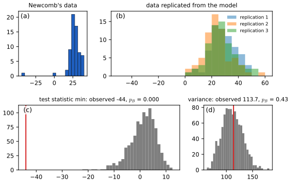
pp. 129–130 For conditional models compare \(p(y\given\bm x_n,\mathcal D)\) to \(y_n\) point by point. The "waffle divorce" example (50 US states, a linear regression of divorce rate on marriage rate and age at first marriage) shows large residuals for Idaho and Utah (many Mormons), with overconfident error bars because the linear model ignores that covariate. That data set is not bundled with any library available here and is not reproduced; the method is that of Figure 3.3, with the predictive plotted against the observed outcome.
3.9.2 Bayesian p-values
pp. 130–131 The posterior predictive (Bayesian) p-value is \[p_B=\Pr(\mathrm{test}(\tilde{\mathcal D})\ge\mathrm{test}(\mathcal D)\given M,\mathcal D)\] (3.320), approximated by \[\frac1S\sum_s\mathbb 1[\mathrm{test}(\tilde{\mathcal D}_s)>\mathrm{test}(\mathcal D)]\] (3.322), whereas the classical p-value \[p_C=\Pr(\mathrm{test}(\tilde{\mathcal D})\ge\mathrm{test}(\mathcal D)\given M)\] (3.321) uses the null model, independent of the data. Values near 0 or 1 signal misfit. A statistic that is sufficient for the model is well fitted, giving \(p_B\approx\frac12\): the Gaussian model cannot represent the support but does represent the variance. Do not ask whether the data come from the model (almost never) but whether it captures the features that matter.
Filling the gap 3.30: the Newcomb p-values in closed form, and the plug-in against the full posterior predictive pp. 128–131, (3.318)–(3.322)
Derivation
Variance (plug-in). Replications are iid \(\mathcal N(\hat\mu,\hat\sigma^2)\), \(N=66\). The sample variance (divisor \(N\)) of a replication is \(\frac{\hat\sigma^2}N\chi^2_{N-1}\). The observed statistic equals \(\hat\sigma^2\) (it is the MLE). Hence \(p_B=\Pr(\chi^2_{65}\ge66)=0.442\) exactly, with no simulation. The book reports 0.48; with \(S=10^3\) replications the Monte Carlo standard error is \(0.016\), so 0.48 is within 2.5 standard errors of the truth. I get 0.4425 with \(2\times10^4\) replications.
Minimum. The observed minimum is \(z=(-44-26.2)/10.66=-6.6\) standard deviations from \(\hat\mu\). A replicated minimum \(\le-44\) needs at least one of 66 draws below \(-6.6\sigma\): \(p_B\le66\,\Phi(-6.6)\approx1.5\times10^{-9}\). So \(p_B\approx0\): the Gaussian model cannot produce such an outlier.
Full Bayes. Replacing the plug-in by draws from the joint posterior under the Jeffreys prior (\(\sigma^2\sim\chi^{-2}(N-1,s^2)\), \[\mu\given\sigma^2\sim\mathcal N(\bar y,\sigma^2/N)\], gap 3.9), the variance \(p_B\) is 0.50 and the minimum \(p_B<0.01\): the same conclusion. The plug-in version slightly understates predictive spread (no parameter uncertainty). Caution: because the data are used twice (to fit and to test), \(p_B\) is not uniformly distributed under the model but concentrates near \(\frac12\) (it is conservative), which is why only extreme values are informative. \(\square\)
3.10 Hypothesis testing
3.10.1 Frequentist approach
p. 131 Null hypothesis significance testing uses a rule \[\delta(\mathcal D)=\mathbb 1[t(\mathcal D)\ge t^*]\] with a critical value \(t^*\) chosen so that \[p(t(\tilde{\mathcal D})\ge t^*\given H_0)=\alpha\] (3.324), controlling the type I error; for the t-statistic \[t(\mathcal D)=\frac{\bar x-\mu}{\hat\sigma/\sqrt N}\] (3.323) this uses the Student law. Equivalent: reject when the p-value (3.86) is below \(\alpha\) (All of Statistics, 10.2). The book avoids NHST because of the problems of Section 3.3.5.2.
3.10.2 Bayesian approach
3.10.2.1–3.10.2.2 Bayes factors; improper priors
pp. 132–133 The Bayes factor of two hypotheses (models) is \[B_{1,0}=\frac{p(\mathcal D\given M_1)}{p(\mathcal D\given M_0)}=\frac{p(M_1\given\mathcal D)/p(M_0\given\mathcal D)}{p(M_1)/p(M_0)}\] (3.325), a likelihood ratio with the parameters integrated out, read on Jeffreys' scale (Table 3.1: \(B_{1,0}>10\) strong, \(>100\) decisive evidence for \(M_1\); \(<\frac1{10}\), \(<\frac1{100}\) for \(M_0\); between \(\frac13\) and 3 weak).
Filling the gap 3.31: the marginalisation paradox for improper priors, and when it does not arise pp. 132–133, (3.326)–(3.327)
Derivation
Let \(p(\theta\given M_i)=c_ih_i(\theta)\) on \(\Theta_i\) where \(h_i\) is a fixed non-integrable function (for example \(h_i\equiv1\) on an unbounded set) and \(c_i>0\) an arbitrary constant: an improper prior is only defined up to a constant. The "marginal likelihood" is \(L_i=c_i\ell_i\), \[\ell_i=\int_{\Theta_i}p(\mathcal D\given\theta)h_i(\theta)\,\d\theta\]. With equal prior model probabilities, \[p(M_0\given\mathcal D)=\frac{c_0\ell_0}{c_0\ell_0+c_1\ell_1}=\frac{\ell_0}{\ell_0+(c_1/c_0)\ell_1}\] (3.327), and the Bayes factor \(B_{1,0}=(c_1/c_0)\ell_1/\ell_0\) is scaled by the arbitrary ratio \(c_1/c_0\): for instance with \(\ell_0=0.8,\ell_1=0.2\), \(p(M_0\given\mathcal D)\) is \(0.8\) for \(c_1=c_0\) but \(0.04\) for \(c_1=100c_0\). For proper priors the constants are fixed by normalisation, so the problem does not arise. It also does not arise for a parameter common to both models given the same improper prior: the constants \(c\) multiply both \(L_0\) and \(L_1\) and cancel from \(B_{1,0}\). This is why the Jeffreys prior \(p(\mu,\sigma)\) on shared nuisance parameters is acceptable in the Bayesian t-test. \(\square\)
3.10.2.3–3.10.2.4 Parameter estimation approach; the binomial test
pp. 133–134 Instead of a Bayes factor, estimate the parameters and ask how much posterior mass lies near the null value: the region of practical equivalence (ROPE), \[\Pr(0.5-\epsilon<\theta<0.5+\epsilon\given\mathcal D)\], and the effect size. For \(y\) successes in \(N\) trials with the flat prior, \(\theta\given\mathcal D\sim\Beta(y+1,N-y+1)\), a credible interval from the posterior quantiles, and \[\Pr(\theta>0.5\given\mathcal D)=\int_{0.5}^1p(\theta\given\mathcal D)\,\d\theta\] (3.328).
3.10.2.5 Two-sample test of proportions
p. 134 With independent \(y_j\sim\Bin(N_j,\theta_j)\), \(\theta_j\sim\Beta(1,1)\), the posteriors are independent betas (3.329) and the difference \(\delta=\theta_1-\theta_2\) has density \[p(\delta\given\mathcal D)=\int_0^1\Beta(\theta_1\given y_1+1,N_1-y_1+1)\Beta(\theta_1-\delta\given y_2+1,N_2-y_2+1)\,\d\theta_1\] (3.330)–(3.331), so \(p(\delta>0\given\mathcal D)\) answers the test.
3.10.2.6–3.10.2.9 Tests of means and a correlation
pp. 134–136 One-sample. Under a noninformative prior the posterior of the mean is the t law (gap 3.9), so the credible interval equals the confidence interval; for robustness the book prefers weakly informative priors, \(\mu\sim\mathcal N(0,2.5\,\mathrm{sd}(y))\), \(\sigma\sim\) half-Student-t, the "Bayesian t-test" (BTT); a Student likelihood with \(\nu-1\sim\mathrm{Expon}(1/29)\) gives the robust BEST test (Kruschke, 2013). Paired: apply BTT to \(y_{2n}-y_{1n}\). Two-sample: \(y_{jn}\sim\mathcal N(\mu_j,\sigma_j^2)\), posterior of \(\mu_2-\mu_1\) (Figure 3.27); allowing \(\sigma_1\ne\sigma_2\) is the Bayesian analogue of Welch's test. Correlation: \((x_n,y_n)\sim\mathcal N(\bm\mu,\Sigma)\) with \(\rho\sim\mathrm{Unif}(-1,1)\), then \(p(\rho>0\given\mathcal D)\).
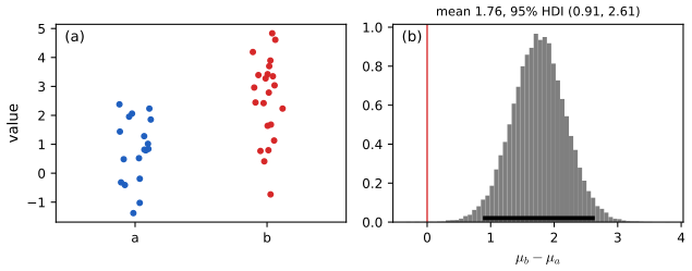
3.10.3 Common statistical tests correspond to inference in linear models
pp. 136–141 Many classical tests are exactly, or approximately, inference on the parameters of a linear model (Table 3.2): one-sample t is an intercept-only regression; paired t is that on the differences; Pearson is simple regression; the pooled two-sample t is a regression on a 0/1 indicator; one-way ANOVA is regression on dummy variables, two-way ANOVA adds interactions. The nonparametric versions are approximated by the same models on ranks (Conover and Iman, 1981): Wilcoxon signed rank \(\leftrightarrow\) signed-rank one-sample t (\(N>14\)), Spearman \(\leftrightarrow\) Pearson on ranks (\(N>10\)), Mann–Whitney \(U\leftrightarrow\) two-sample t on signed ranks (\(N>11\)), Kruskal–Wallis \(\leftrightarrow\) one-way ANOVA on ranks (\(N>11\)). The rank transform of \((3.6,3.4,-5.0,8.2)\) is \((3,2,1,4)\), the signed rank transform \((2,1,-3,4)\).
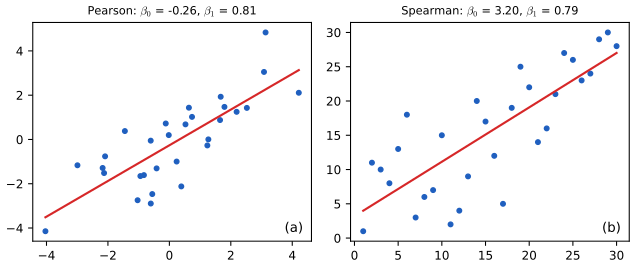
Filling the gap 3.32: the one- and two-sample t-tests and one-way ANOVA as regressions pp. 137–139, (3.334)–(3.338)
Derivation
One sample. The model \(y_n=\beta_0+\varepsilon_n\) has design matrix \(\bm 1\), so \(\hat\beta_0=\bar y\), \(\mathrm{RSS}=\sum(y_n-\bar y)^2\), \(\widehat{\mathrm{se}}(\hat\beta_0)=s/\sqrt N\) with \(s^2=\mathrm{RSS}/(N-1)\); the regression t-statistic \(\hat\beta_0/\widehat{\mathrm{se}}\) is \(t=\bar y/(s/\sqrt N)\) (3.323) with \(N-1\) degrees of freedom. Paired data: apply this to \(y_{2n}-y_{1n}\).
Two samples. With \(x_n\in\{0,1\}\) and \(y_n=\beta_0+\beta_1x_n+\varepsilon_n\), \(\hat\beta_0=\bar y_0\), \(\hat\beta_1=\bar y_1-\bar y_0\), and \[(\bm X^\T\bm X)^{-1}_{11}=\frac1{N_0}+\frac1{N_1}\], RSS is the pooled within-group sum of squares, so \[t=\frac{\bar y_1-\bar y_0}{s_p\sqrt{1/N_0+1/N_1}}\], the pooled two-sample t statistic with \(N-2\) degrees of freedom. Welch's test uses \(\var(y_n)=\sigma_x^2\) depending on the group (heteroscedastic regression).
ANOVA. Dummy coding \(x[j]=\mathbb 1[x=j]\), dropping level 1 (reduced rank, to avoid the collinearity \(\sum_jx[j]=1\)): \[f_{\rm aov}(x,\beta)=\beta_0+\sum_{j\ge2}\beta_jx[j]\] (3.335); \(\beta_0\) is the mean of level 1 and \(\beta_j=\mu_j-\mu_1\). The null \(\mu_1=\dots=\mu_J\) is \(\beta_2=\dots=\beta_J=0\), tested by the regression F-statistic \[F=\frac{(\mathrm{RSS}_0-\mathrm{RSS}_1)/(J-1)}{\mathrm{RSS}_1/(N-J)}\], where \(\mathrm{RSS}_0\) is the total sum of squares (the intercept-only fit), \[\mathrm{RSS}_0-\mathrm{RSS}_1=\sum_jN_j(\bar y_j-\bar y)^2\] the between-group and \[\mathrm{RSS}_1=\sum_j\sum_i(y_{ij}-\bar y_j)^2\] the within-group sum of squares: the classical ANOVA F. Numerical confirmation: the regression F test and f_oneway agree to machine precision. Symmetric form. The constrained form \(\beta_0+\sum_{j=1}^J\beta_jx[j]\) with \(\sum_j\beta_j=0\) (3.336) is obtained from unconstrained effects \(\tilde\beta_j\) by \(\beta_j=\tilde\beta_j-\bar{\tilde\beta}\), \(\beta_0=\tilde\beta_0+\bar{\tilde\beta}\) (3.337): then \[\sum_j\beta_j=J\bar{\tilde\beta}-J\bar{\tilde\beta}=0\] (3.338) and the mean function \[\beta_0+\sum_j\beta_jx[j]=\tilde\beta_0+\sum_j\tilde\beta_jx[j]\] is unchanged (since \(\sum_jx[j]=1\)). A Bayesian version puts a prior on \(\bm\beta\), allows group-specific variances and a Student likelihood (Section 3.6). \(\square\)
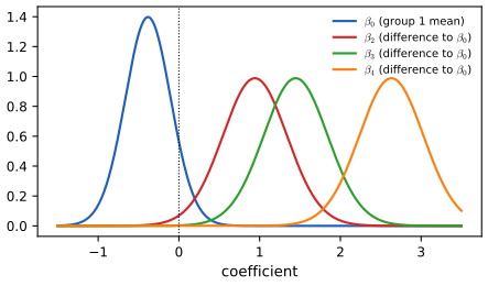
Filling the gap 3.33: correlation as a regression slope, and the correction needed for scaling pp. 137–138, Section 3.10.3.3
Derivation
For simple regression \(y_n=\beta_0+\beta_1x_n+\varepsilon_n\) the least squares slope is \(\hat\beta_1=S_{xy}/S_{xx}=r\,\frac{s_y}{s_x}\), where \(r\) is the sample correlation. The book says that scaling \(y\) to unit standard deviation gives \(\beta_1=\rho\). That requires \(s_x=1\) as well: scaling only \(y\) gives \(\hat\beta_1=r/s_x\). Scaling both gives \(\hat\beta_1=r\) exactly. Numerically (60 points, \(s_x\approx2\)) scaling only \(y\) gave a slope far from \(r\) and equal to \(r/s_x\). A test of \(\rho=0\) is a test of \(\beta_1=0\): \(\mathrm{RSS}=(1-r^2)S_{yy}\), \[\widehat{\mathrm{se}}^2(\hat\beta_1)=\frac{\mathrm{RSS}/(N-2)}{S_{xx}}\], so \[t=\frac{\hat\beta_1}{\widehat{\mathrm{se}}}=r\sqrt{\frac{N-2}{1-r^2}}\], the classical t-test of a correlation. The Spearman coefficient is by definition the Pearson correlation of the ranks, so regression on ranks (Figure 3.28) tests it; scipy's Spearman correlation and the Pearson correlation of the ranks agree to \(10^{-10}\). The rank-based approximations are good: over 300 simulated samples the median absolute difference between the Wilcoxon p-value (\(N=30\)) and the p-value of the t-test on signed ranks was 0.0018, and 0.0021 for Mann–Whitney against the t-test on ranks (\(N=20,22\)). With several predictors the posterior of a partial correlation follows from that of the regression weights. \(\square\)
3.10.3.5–3.10.3.7 Multi-way ANOVA, counts, non-metric outputs
pp. 139–141 Two nominal predictors have mean function \[\mu+\sum_j\alpha_jx_{1[j]}+\sum_k\beta_kx_{2[k]}+\sum_{jk}\gamma_{jk}x_{1[j]}x_{2[k]}\] with sum-to-zero constraints (3.339)–(3.340); "no interaction" is \(\gamma=0\). For counts in an \(R\times C\) contingency table (Table 3.3: handedness against sex, \[\begin{pmatrix}9&43\\4&44\end{pmatrix}\]) the \(\chi^2\) test of independence uses \[\chi^2=\sum_{r,c}\frac{(O_{rc}-E_{rc})^2}{E_{rc}}\], \(E_{rc}=Np_{r\cdot}p_{\cdot c}\) (3.341); the Bayesian/GLM version is a Poisson model \(y\sim\mathrm{Poi}(\lambda_{rc})\), \[\lambda_{rc}=\exp(\beta_0+\beta_r+\beta_c+\beta_{rc})\] (3.342)–(3.343), independence being \(\beta_{rc}=0\). For categorical or ordinal or count outputs use logistic, ordinal or Poisson regression (Chapter 15).
Filling the gap 3.34: the \(\chi^2\) test of independence as a Poisson log-linear model pp. 140–141, (3.341)–(3.343)
Derivation
Fit under independence. The Poisson log likelihood of the model \(\log\lambda_{rc}=\beta_0+\beta_r+\beta_c\) (no interaction) is \[\sum_{rc}(O_{rc}\log\lambda_{rc}-\lambda_{rc})\]. Setting the derivative with respect to \(\beta_r\) to zero gives \(\sum_cO_{rc}=\sum_c\lambda_{rc}\) (row totals matched), and likewise for columns. The unique solution is \[\hat\lambda_{rc}=O_{r\cdot}O_{\cdot c}/N=E_{rc}\] (check: row sums \(\sum_cO_{r\cdot}O_{\cdot c}/N=O_{r\cdot}\)). So the fitted counts are exactly the expected counts of (3.341); the full interaction model fits \(\hat\lambda_{rc}=O_{rc}\).
Likelihood ratio versus Pearson. The deviance of the independence model against the saturated one is \(G^2=2\sum O_{rc}\log(O_{rc}/E_{rc})\). With \(\delta=O-E\) and \(\sum\delta=0\), \[(E+\delta)\log(1+\delta/E)=\delta+\frac{\delta^2}{2E}+O(\delta^3/E^2)\], so \[G^2=\sum_{rc}\frac{\delta_{rc}^2}{E_{rc}}+\ldots=\chi^2+\ldots\]: the two statistics agree to second order, and both are asymptotically \(\chi^2\) with \((R-1)(C-1)\) degrees of freedom. For Table 3.3: \(\chi^2=1.777\) (\(p=0.18\), one degree of freedom) and the Poisson deviance \(G^2=1.825\); the fitted values of the Poisson model equal the expected counts. A Bayesian analysis would instead report the posterior of \(\beta_{rc}\). \(\square\)
3.11 Missing data
pp. 141–142 Let \(X_n=(X_{n,{\rm obs}},X_{n,{\rm mis}})\) and let \(R_n\) indicate which components are revealed (\(R_{n,{\rm obs}}=1\)). The mechanism is MCAR if \(p(R_n\given X_n)=p(R_n)\), MAR if \(p(R_n\given X_n)=p(R_n\given X_{n,{\rm obs}})\), and MNAR otherwise (Rubin, 1976). For a discriminative model \(p(y_n\given\bm x_n,\theta)\) with some labels missing (Figure 3.30), unlabelled points can be ignored under MCAR and MAR because \(\theta\) is unaffected by a hidden leaf \(y_n\); under MNAR \(\theta\) is coupled to \(y_n\) through \(r_n\), so the missing values must be imputed (Section 20.3.3). For a generative model \(p(\bm x,y)=p(y)p(\bm x\given y)\) the unlabelled points inform \(\theta\) even under MCAR and MAR, the basis of semi-supervised learning.
Filling the gap 3.35: when can the missingness mechanism be ignored? pp. 141–142, Figure 3.30
Derivation
Let the data model have parameters \(\theta\) and the mechanism have parameters \(\phi\), \(p(\bm r\given\bm x,\phi)\). The observed-data likelihood integrates out the hidden entries: \[p(\bm x_{\rm obs},\bm r\given\theta,\phi)=\int p(\bm x_{\rm obs},\bm x_{\rm mis}\given\theta)\,p(\bm r\given\bm x_{\rm obs},\bm x_{\rm mis},\phi)\,\d\bm x_{\rm mis}\]. Under MAR the second factor does not depend on \(\bm x_{\rm mis}\), so it comes out of the integral: \[ p(\bm x_{\rm obs},\bm r\given\theta,\phi)=p(\bm r\given\bm x_{\rm obs},\phi)\int p(\bm x_{\rm obs},\bm x_{\rm mis}\given\theta)\,\d\bm x_{\rm mis}=p(\bm r\given\bm x_{\rm obs},\phi)\,p(\bm x_{\rm obs}\given\theta). \] The likelihood factorises into a part for \(\theta\) and a part for \(\phi\); if \(\theta\) and \(\phi\) are distinct (a priori independent) the posterior of \(\theta\) is the same with or without modelling \(\bm r\): the mechanism is ignorable. MCAR is a special case. Under MNAR \[p(\bm r\given\bm x_{\rm obs},\bm x_{\rm mis},\phi)\] depends on \(\bm x_{\rm mis}\), the integral does not factorise, and ignoring \(\bm r\) biases inference. In the conditional model with labels \(y_n\) missing, a hidden \(y_n\) (MCAR or MAR given \(\bm x_n\)) contributes \(\int p(y_n\given\bm x_n,\theta)\,\d y_n=1\) to the likelihood, so only labelled pairs matter. Simulation (\(y=1+2x+\epsilon\), \(2\times10^5\) points, labels revealed with probability \(\frac12\) (MCAR), \(\sigma(2x)\) (MAR) or \(\sigma(2(y-1))\) (MNAR)): the complete-case least squares slope and intercept are \((2.00,1.00)\) under MCAR, \((2.00,1.00)\) under MAR and a biased \((1.61,1.59)\) under MNAR. \(\square\)
Practice problems
The book has no end-of-chapter exercises for this chapter. Three practice problems, with complete solutions (hidden); the numbers are computed with the code of this chapter. Labelled \(P\) to avoid confusion with the book's numbering.
Problem P1 (Jeffreys prior for a Poisson rate). Let \[y_1,\dots,y_N\overset{\rm iid}\sim\mathrm{Poi}(\lambda)\] with \(S=\sum_ny_n\). (a) Find the Fisher information \(F(\lambda)\), the Jeffreys prior and the posterior. (b) Compute the posterior means for \(N=4\), \(S=6\) under the flat prior on \(\lambda\), the flat prior on \(\log\lambda\) and the Jeffreys prior. (c) Show directly that the Jeffreys prior in the parameter \(\varphi=\sqrt\lambda\) is flat.
Solution
(a) \[\log p(y\given\lambda)=y\log\lambda-\lambda-\log y!\], score \(y/\lambda-1\), \(F_1(\lambda)=\var(y)/\lambda^2=1/\lambda\) (or \(-\E[-y/\lambda^2]\)), so \(F(\lambda)=N/\lambda\) for \(N\) observations and \(p_J(\lambda)\propto\lambda^{-1/2}\). The posterior \(\propto\lambda^{S}e^{-N\lambda}\lambda^{-1/2}\) is \(\mathrm{Gamma}(S+\frac12,N)\) (shape, rate).
(b) Likelihood \(\lambda^Se^{-N\lambda}\). Flat in \(\lambda\): \(\mathrm{Gamma}(S+1,N)\), mean \((S+1)/N=1.75\). Flat in \(\log\lambda\), i.e. \(p(\lambda)\propto1/\lambda\): \(\mathrm{Gamma}(S,N)\), mean \(S/N=1.5\). Jeffreys: \(\mathrm{Gamma}(S+\frac12,N)\), mean \((S+\frac12)/N=1.625\). The three differ, and only the Jeffreys answer is the same whichever parameterisation one starts from.
(c) With \(\varphi=\sqrt\lambda\), \(\lambda=\varphi^2\), \[F_\varphi=F_\lambda(\d\lambda/\d\varphi)^2=\frac N{\varphi^2}(2\varphi)^2=4N\], constant, so the Jeffreys prior \(\sqrt{F_\varphi}\) is flat in \(\varphi\); in \(\lambda\) it is \[|\d\varphi/\d\lambda|=\frac1{2\sqrt\lambda}\propto\lambda^{-1/2}\], as in (a). (The demonstration "Jeffreys priors and reparameterisation", preset 4, reproduces the three means.) \(\square\)
Problem P2 (shrinkage in the eight schools). For school 0 (\(y_0=28,\sigma_0=15\)) and school 7 (\(y_7=12,\sigma_7=18\)), take \(\tau=5\) and \(\mu=4.5\) as fixed. Compute \(w_j\), the posterior mean and the posterior standard deviation of \(\theta_j\). Which school is shrunk more, and why?
Solution
By gap 3.19, \(w_j=\frac{\sigma_j^2}{\sigma_j^2+\tau^2}\), posterior mean \(w_j\mu+(1-w_j)y_j\), variance \((1-w_j)\sigma_j^2\). School 0: \(w_0=\frac{225}{250}=0.9\), mean \(0.9\cdot4.5+0.1\cdot28=6.85\), variance \(0.1\cdot225=22.5\), sd \(4.74\). School 7: \(w_7=\frac{324}{349}=0.9284\), mean \(0.9284\cdot4.5+0.0716\cdot12=5.04\), variance \(0.0716\cdot324=23.2\), sd \(4.82\). School 7 is shrunk more (weight 0.928 on the population mean against 0.900) because its observation is noisier (\(\sigma_7>\sigma_0\)), so the data are given less weight relative to the population distribution; but school 0 moves further in absolute terms (from 28 to 6.85) because its observation was far from \(\mu\). \(\square\)
Problem P3 (a normal inverse chi-squared update). Observe \(y=(2.1,3.4,1.9,2.8,3.3)\) with the prior \[\NIX(\breve m=2,\breve\kappa=1,\breve\nu=2,\breve\tau^2=1)\]. Find the posterior parameters, \(\E[\sigma^2\given\mathcal D]\) and a 95% credible interval for \(\mu\).
Solution
\(N=5\), \(\bar y=2.7\), \[S=\sum(y_n-\bar y)^2=0.36+0.49+0.64+0.01+0.36=1.86\]. By (3.121)–(3.124): \(\hat\kappa=6\), \(\hat\nu=7\), \(\hat m=\frac{1\cdot2+5\cdot2.7}6=2.5833\), \[\hat\nu\hat\tau^2=2\cdot1+1.86+\frac{5\cdot1}6(2-2.7)^2=4.2683\], so \(\hat\tau^2=0.6098\). Then \[\E[\sigma^2\given\mathcal D]=\frac{\hat\nu}{\hat\nu-2}\hat\tau^2=\frac75\cdot0.6098=0.854\]. The marginal of \(\mu\) is \(T(2.5833,\hat\tau^2/\hat\kappa=0.1016,7)\): the interval is \[2.5833\pm t_{7,0.975}\sqrt{0.1016}=2.5833\pm2.3646\cdot0.3188=(1.83,3.34)\]. \(\square\)
Demonstrations
| Page | What it shows | In the notes |
|---|---|---|
| Partial pooling | The eight-schools posterior of τ, shrinkage weights and full-Bayes means, and empirical Bayes for the 71 rat tumour groups. Presets: 1 eight schools, full Bayes; 2 complete pooling; 3 no pooling; 4 rats, empirical Bayes; 5 rats, a very strong prior. | 3.6, 3.7, gap 3.19, 3.21 |
| Jeffreys priors and reparameterisation | Flat-in-θ, flat-in-φ and Jeffreys posteriors for a binomial rate, a Poisson rate and a Gaussian scale, with the Fisher information of the new parameterisation computed numerically. Presets: 1 binomial odds (Fig 3.13); 2 log-odds; 3 arcsine; 4 Poisson log rate; 5 Gaussian log scale. | 3.5.2, gap 3.16 |
| Evidence, BIC, AIC, LOO and WAIC | Degree selection for Bayesian polynomial regression with a known noise level and a prior precision you can change. Presets: 1 the fixed sample; 2 too much assumed noise; 3 a vague prior; 4 a large sample; 5 a small noisy sample. | 3.8, gaps 3.27–3.29 |
The Python code that produces every computed figure of this page is code/ch03_statistics.py (see the code index). Companion demos: the beta-binomial model, conjugate priors, bootstrap replicates.
Notes on the book
Points where the book is imprecise or wrong
- (3.62) and (3.234). The entries of the displayed Fisher information matrix for the Gaussian lack the minus signs of \(-\E[\partial^2\ell]\); and (3.234) is introduced for \(\theta=(\mu,\sigma)\) but is the information for \((\mu,\sigma^2)\) (the information for \((\mu,\sigma)\) is \(\diag(1/\sigma^2,2/\sigma^2)\)). The "standard Jeffreys prior" (3.235), \(1/\sigma^2\), is the product of one-dimensional Jeffreys priors; the joint Jeffreys prior for \((\mu,\sigma^2)\) is \(\sigma^{-3}\) (gap 3.16).
- Section 3.4.6.2. The Gaussian prior is written \(\mathcal N(\theta\given0,2.19^2)\); the quoted posterior mean 3.43 requires the variance to be 2.19 (the variance \(2.19^2\) would give 4.14), gap 3.12.
- (3.166). The exponent of \(|\Sigma|\) lost its minus sign: it is \(-(\hat\nu+D+2)/2\) (gap 3.10).
- (3.178)–(3.180). The text concludes that \(\hat\Psi\) is the maximiser; the correct maximiser, stated in (3.180), is \(\hat\Psi/(\hat\nu+D+2)\). The derivative written in (3.178) is that of \(-2\log p\) (gap 3.10).
- (3.217). The LKJ density on the Cholesky factor has factor \(\prod_iL_{ii}^{D-i+2\eta-2}\); the printed \(|L|^{-\eta-1}\) does not match (3.216) even for \(D=2\) (gap 3.14).
- (3.284). The harmonic mean estimator needs samples from the posterior \(p(\theta\given\mathcal D)\), as the sentence says, not from the prior as the formula's annotation \(\theta_s\sim p(\theta)\) states. Section 3.8.3.4 writes "\(\log q(\mathcal D\given\theta)\)" for the evidence lower bound.
- Section 3.9.2. The Bayesian p-value of the variance in Newcomb's data is quoted as 0.48; its exact value under the plug-in model is \(\Pr(\chi^2_{65}\ge66)=0.442\), and a simulation of size 1000 has standard error 0.016 (gap 3.30).
- Section 3.10.3.3. "If we scale \(Y\) to have standard deviation 1 then \(\beta_1=\rho\)" needs \(X\) scaled to unit standard deviation as well; scaling only \(Y\) gives \(\rho/\mathrm{sd}(X)\) (gap 3.33). In Section 3.8.6 the threshold \(k_n>0.5\) is the point where the variance of the weights becomes infinite; the usual practical warning level is 0.7.
- Supplement (S3.26). The factor \(g(\eta)e^{-\psi(y)}\) should read \(g(\eta)e^{-\psi(\eta)}\) (gap 3.39).
- Supplement Section 3.1.1.5. After \(\{16,8,2,64\}\) the maximum likelihood hypothesis is "powers of 2 except 32" when the space contains it, not "powers of two" (gap 3.36).
- Section 3.4.3.4 and (3.128). The "\(\NIX\) with \(\breve\nu=-1\)" is an improper limit, valid only formally (its posterior is proper for \(N\ge2\); the variance (3.132) exists for \(N>3\)). Not an error, but the formulas should be read with these conditions.
References
- Murphy, K. P. (2023). Probabilistic Machine Learning: Advanced Topics. MIT Press, Cambridge, MA. Chapter 3 and Supplement Chapter 3. probml.github.io/pml-book/book2.html.
- Akaike, H. (1974). A new look at the statistical model identification. IEEE Transactions on Automatic Control, 19(6), 716–723.
- Berger, J. O. (1985). Statistical Decision Theory and Bayesian Analysis, 2nd edition. Springer, New York.
- Bernardo, J. M. (1979). Reference posterior distributions for Bayesian inference. Journal of the Royal Statistical Society, Series B, 41(2), 113–147.
- Betancourt, M. and Girolami, M. (2015). Hamiltonian Monte Carlo for hierarchical models. In Current Trends in Bayesian Methodology with Applications, CRC Press, 79–101.
- Clarke, B. S. and Barron, A. R. (1994). Jeffreys' prior is asymptotically least favorable under entropy risk. Journal of Statistical Planning and Inference, 41(1), 37–60.
- Conover, W. J. and Iman, R. L. (1981). Rank transformations as a bridge between parametric and nonparametric statistics. The American Statistician, 35(3), 124–129.
- de Finetti, B. (1937). La prévision: ses lois logiques, ses sources subjectives. Annales de l'Institut Henri Poincaré, 7, 1–68.
- Diaconis, P. and Freedman, D. (1980). Finite exchangeable sequences. Annals of Probability, 8(4), 745–764.
- Diaconis, P. and Ylvisaker, D. (1979). Conjugate priors for exponential families. Annals of Statistics, 7(2), 269–281.
- Efron, B. (1979). Bootstrap methods: another look at the jackknife. Annals of Statistics, 7(1), 1–26.
- Efron, B. (2011). Tweedie's formula and selection bias. Journal of the American Statistical Association, 106(496), 1602–1614.
- Gelman, A. (2006). Prior distributions for variance parameters in hierarchical models. Bayesian Analysis, 1(3), 515–534.
- Gelman, A., Carlin, J. B., Stern, H. S., Dunson, D. B., Vehtari, A. and Rubin, D. B. (2014). Bayesian Data Analysis, 3rd edition. CRC Press, Boca Raton, FL.
- Griffiths, T. L. and Tenenbaum, J. B. (2006). Optimal predictions in everyday cognition. Psychological Science, 17(9), 767–773.
- Jaynes, E. T. (2003). Probability Theory: The Logic of Science. Cambridge University Press.
- Jeffreys, H. (1946). An invariant form for the prior probability in estimation problems. Proceedings of the Royal Society A, 186, 453–461.
- Kruschke, J. K. (2013). Bayesian estimation supersedes the t test. Journal of Experimental Psychology: General, 142(2), 573–603.
- Lewandowski, D., Kurowicka, D. and Joe, H. (2009). Generating random correlation matrices based on vines and extended onion method. Journal of Multivariate Analysis, 100(9), 1989–2001.
- Lotfi, S., Izmailov, P., Benton, G., Goldblum, M. and Wilson, A. G. (2022). Bayesian model selection, the marginal likelihood, and generalization. International Conference on Machine Learning.
- MacKay, D. J. C. and Peto, L. C. B. (1995). A hierarchical Dirichlet language model. Natural Language Engineering, 1(3), 289–308.
- Minka, T. P. (2000). Estimating a Dirichlet distribution. Technical report, MIT.
- Nalisnick, E. and Smyth, P. (2018). Learning priors for invariance. Artificial Intelligence and Statistics.
- Rubin, D. B. (1976). Inference and missing data. Biometrika, 63(3), 581–592.
- Rubin, D. B. (1984). Bayesianly justifiable and relevant frequency calculations for the applied statistician. Annals of Statistics, 12(4), 1151–1172.
- Schwarz, G. (1978). Estimating the dimension of a model. Annals of Statistics, 6(2), 461–464.
- Sellke, T., Bayarri, M. J. and Berger, J. O. (2001). Calibration of p values for testing precise null hypotheses. The American Statistician, 55(1), 62–71.
- Tenenbaum, J. B. (1999). A Bayesian framework for concept learning. PhD thesis, MIT.
- Vehtari, A., Gelman, A. and Gabry, J. (2017). Practical Bayesian model evaluation using leave-one-out cross-validation and WAIC. Statistics and Computing, 27(5), 1413–1432.
- Wasserman, L. (2004). All of Statistics. Springer, New York.
- Watanabe, S. (2010). Asymptotic equivalence of Bayes cross validation and widely applicable information criterion in singular learning theory. Journal of Machine Learning Research, 11, 3571–3594.
The numerical statements in the text (the conjugate updates, the HPD and central intervals, the mixture-of-betas probabilities, the Fisher information formulas, the Jeffreys posteriors, the eight-schools and rat-tumour posteriors and empirical Bayes fits, the evidence, BIC, AIC, LOO and WAIC computations, the Newcomb p-values, the equivalences between tests and linear models, the missing-data simulation and the number-game and taxicab results) were confirmed numerically against independent computations, and the three demonstration pages against the Python code.