Energy-based models
An energy-based model (EBM) defines a density by a free-form energy function, \(p_{\bm\theta}(\bm x)=e^{-E_{\bm\theta}(\bm x)}/Z_{\bm\theta}\), and pays for that freedom with an intractable normalising constant. These notes follow the chapter's three families of remedies: maximum likelihood with MCMC (Langevin sampling, contrastive divergence, persistent chains), the methods that never touch \(Z_{\bm\theta}\) (score matching in its basic, denoising and sliced forms, and noise contrastive estimation), and the divergence-based and adversarial alternatives. Beyond the book, the notes prove the exact bias of discretised Langevin dynamics, show that contrastive divergence is a KL between a reconstruction posterior and a reversed kernel, give closed-form solutions of score matching for energies that are linear in their parameters, derive the NCE gradient as a reweighted likelihood gradient, and correct several equations and one algorithm of the draft.
Ch. 1 Introduction Ch. 2 Probability Ch. 3 Statistics Ch. 4 Graphical models Ch. 5 Information theory Ch. 6 Optimisation Ch. 7 Inference algorithms Ch. 8 Gaussian filtering Ch. 9 Message passing Ch. 10 Variational inference Ch. 11 Monte Carlo Ch. 12 MCMC Ch. 13 Sequential Monte Carlo Ch. 14 Predictive models Ch. 15 GLMs Ch. 16 Deep networks Ch. 17 Bayesian neural networks Ch. 18 Gaussian processes Ch. 19 Beyond iid Ch. 20 Generative models Ch. 21 VAEs Ch. 22 Autoregressive models Ch. 23 Normalizing flows Ch. 24 Energy-based models Ch. 25 Diffusion models Ch. 26 GANs Ch. 27 Discovery methods Ch. 28 Latent factor models Ch. 29 State-space models Ch. 30 Graph learning Ch. 31 Nonparametric Bayes Ch. 32 Representation learning Ch. 33 Interpretability Ch. 34 Decision making Ch. 35 Reinforcement learning Ch. 36 Causality
How to read these notes
They follow the book. Sections carry the book's numbers, and equations the book numbers keep their numbers, e.g. \((24.15)\); equations without a number are steps the book skips. The supplement for Chapter 24 contains no sections in this draft (its chapter page is empty), so there are no supplement sections to place.
Filling the gaps. Wherever the book writes "one can show", quotes a result from the literature, or leaves a step to the reader, an orange Filling the gap box gives the full argument. Proofs start hidden: open one with its bar, or use the buttons below. Results already proved elsewhere on the site (the RBM conditionals, free energy and clamped-minus-unclamped gradient; the Langevin diffusion, MALA and the bias of ULA; Tweedie's formula; annealed importance sampling; the Bregman form of the KL divergence) are stated and linked rather than repeated.
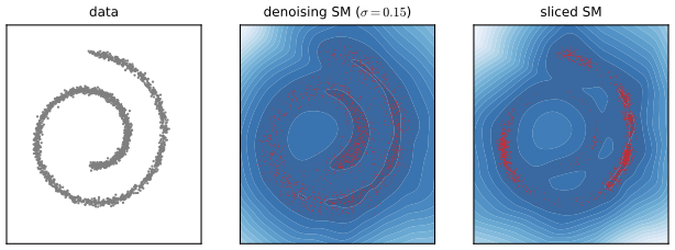
Figures, scale and demonstrations. Every computed figure is reproduced by the Python code. The book's Figure 24.1 draws two energies and their sum with sampled trajectories; the one here uses my own two energies in the same spirit. Figure 24.2 is a schematic of contrastive divergence in an RBM and is not reproduced. The book has no data set in this chapter; everything below is simulation or the 8 × 8 digits bundled with scikit-learn, and every network is small and trained on the CPU in seconds to a minute. Seven extra figures (24.x1 to 24.x7) illustrate results proved here; the text of Section 24.3 points to a swiss-roll example in Chapter 25, and Figure 24.x7 is my own version of that kind of example. The ▶ Demo boxes open an interactive demonstration set to the case being discussed.
Main reference
K. P. Murphy, Probabilistic Machine Learning: Advanced Topics, MIT Press (2023; online draft of December 2025), Chapter 24 (with Yang Song and Durk Kingma), pages 849–865 (book page: probml.github.io/pml-book/book2.html), and the supplementary material, Chapter 24. Section, equation, figure and algorithm numbers below refer to this book. The explanations, derivations, figures and code are my own. The book has no end-of-chapter exercises for this chapter; three practice problems are given instead.
Companion courses
Earlier chapters of this course supply most of the tools: undirected models and the RBM (Section 4.3.3.2, gap 4.11, gap 4.19), Tweedie's formula (gap 3.39), KL, Bregman divergences and mutual-information bounds (gap 5.10, gap 5.17), annealed importance sampling for the partition function (gap 11.10), and Langevin dynamics, MALA and the bias of ULA (Section 12.5.6, gap 12.14). The other deep generative models are in Chapter 20 (overview) and Chapter 21 (VAEs); in the deep-learning course see normalizing flows and diffusion models (the continuation of Section 24.3.5), and in the Bishop course the chapter on sampling methods.
What this chapter adds: the regularity conditions and Hessian behind the gradient of \(\log Z\), the exact stationary variance and stability limit of discretised Langevin dynamics, the identity \(\mathrm{CD}_1=\E_y\Dkl(p(x\given y)\|r(x\given y))\), a bound on the tracking error of persistent chains, the closed-form score-matching and denoising-score-matching solutions for energies linear in their parameters, the bias and variance of DSM, the corrected sliced objective and the variances of its trace estimators, the corrected one-step-Langevin and de Bruijn identities, the NCE gradient as a reweighted likelihood gradient, the identifiability gap in the NCE-to-SM argument, the Stein identity and kernelised Stein discrepancy, and the exact slack of the adversarial bound.
The chapter at a glance
- 24.1 Sums of energies are products of densities (gap 24.1).
- 24.2 The likelihood gradient needs a model expectation (gap 24.2); Langevin sampling and its step-size limits (gap 24.3); the RBM and CD-1 (gap 24.4); what CD optimises and where it is biased (gap 24.5); persistent chains (gap 24.6).
- 24.3 Score matching and its closed form (gap 24.7); DSM, Tweedie, bias and variance (gap 24.8); the sliced objective with its correct sign (gap 24.9); the link with CD and the de Bruijn identity (gap 24.10); conservative fields (gap 24.16).
- 24.4 NCE: consistency, gradient and the choice of noise (gap 24.11); NCE as sliced score matching (gap 24.12).
- 24.5 KL contraction (gap 24.13); the Stein discrepancy (gap 24.14); the adversarial bound (gap 24.15).
Notation. \(\bm x\) is the data, \(E_{\bm\theta}\) the energy, \(Z_{\bm\theta}=\int e^{-E_{\bm\theta}}\d\bm x\) the partition function, \(p_{\mathcal D}\) the data distribution, \(\sc_{\bm\theta}(\bm x)=\nabla_{\bm x}\log p_{\bm\theta}(\bm x)=-\nabla_{\bm x}E_{\bm\theta}(\bm x)\) the (Stein) score, and \(\DF(p\|q)=\E_p[\frac12\|\nabla\log p-\nabla\log q\|^2]\) the Fisher divergence (24.28), with the factor \(\frac12\) included.
Prerequisites. Chapters 4, 5, 11 and 12 of the book.
24.1 Introduction
p. 849 The generative models of the previous chapters are directed: the data are generated one step at a time with locally normalised conditionals. Sometimes it is easier to say which configurations are acceptable than how to generate them. An energy-based model is the Gibbs distribution \[ p_{\bm\theta}(\bm x)=\frac{e^{-E_{\bm\theta}(\bm x)}}{Z_{\bm\theta}} \tag{24.1} \] \[ Z_{\bm\theta}=\int e^{-E_{\bm\theta}(\bm x)}\,\d\bm x \tag{24.2} \] where \(Z_{\bm\theta}\) is constant in \(\bm x\) but depends on \(\bm\theta\) and is usually intractable (Section 11.5.4.1 treats annealed importance sampling, gap 11.10). The energy can be any network that returns a real number, with one requirement: \(Z_{\bm\theta}\) must be finite. The book says the energy "returns a non-negative scalar"; that is not needed (an energy can be negative, and adding a constant to \(E\) only rescales \(Z\)), see the notes on the book.
24.1.1 Example: products of experts (PoE)
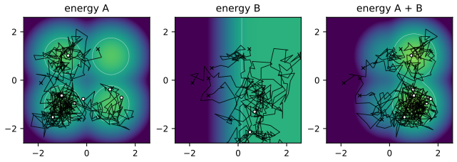
pp. 849–850 Suppose \(p_1\) generates thermally stable proteins and \(p_2\) proteins that bind a target. Neither alone is the model we want, but their product of experts (Hinton 2002) \[ p_{12}(\bm x)=\frac{1}{Z_{12}}p_1(\bm x)p_2(\bm x) \tag{24.3} \] gives high probability only to what both experts like, whereas a mixture would produce either kind of protein but never the conjunction. If the experts are EBMs the product is an EBM with \[ E_{12}(\bm x)=E_1(\bm x)+E_2(\bm x) \tag{24.4} \] so each energy acts as a soft constraint. The book illustrates this in 2-D with Figure 24.1; the figure below uses two energies of my own: expert A has four Gaussian wells at \((\pm1,\pm1)\), and expert B is the soft constraint "\(x_1>0\)", \(E_B=\log(1+e^{-5x_1})\).
Filling the gap 24.1: why summing energies multiplies densities, the Gaussian product, the difference from a mixture, and an improper expert pp. 849–850, (24.3)–(24.4)
Proof
Energies add. Write \(p_i\propto e^{-E_i}\) (the \(E_i\) need not be normalised). Then \(p_1p_2\propto e^{-(E_1+E_2)}\), and the product is a probability density exactly when \(Z_{12}=\int e^{-E_1-E_2}\d\bm x<\infty\). Neither expert has to be normalisable by itself: expert B above has \(\int e^{-E_B}=\int(1+e^{-5x_1})^{-1}\d\bm x=\infty\), yet the product with the proper expert A is perfectly proper because A supplies the decay.
The Gaussian case. For \(p_i\propto\N(x;m_i,v_i)\) in 1-D, complete the square: \[ -\frac{(x-m_1)^2}{2v_1}-\frac{(x-m_2)^2}{2v_2}=-\frac{(x-m)^2}{2v}+\mathrm{const},\qquad \frac1v=\frac1{v_1}+\frac1{v_2},\quad m=v\Big(\frac{m_1}{v_1}+\frac{m_2}{v_2}\Big), \] so precisions add and the product has smaller variance than either expert, \(v<\min(v_1,v_2)\). With \(v_1=2\), \(v_2=\frac12\) this gives \(v=0.4\), whereas the equal mixture of the same two Gaussians has variance \(\frac12(v_1+v_2)+\frac14(m_1-m_2)^2\ge\frac12(v_1+v_2)\), here 1.81 for \(m_1-m_2=1.5\) (both numbers were confirmed by quadrature). A product is a conjunction (it sharpens), a mixture a disjunction (it spreads). The normaliser of two normalised Gaussians is \(Z_{12}=\N(m_1;m_2,v_1+v_2)\), the density of the difference of the means: the experts must agree for the product to have much mass.
The example of Figure 24.1. Since \(e^{-E_B(\bm x)}=1/(1+e^{-5x_1})=\sigm(5x_1)\), the product is expert A reweighted by the logistic "probability that the constraint holds", \[ p_{AB}(\bm x)=\frac{p_A(\bm x)\,\sigm(5x_1)}{\E_{p_A}[\sigm(5x_1)]},\qquad \E_{p_A}[\sigm(5x_1)]=\tfrac12 \] by symmetry of \(p_A\) in \(x_1\) and \(\sigm(t)+\sigm(-t)=1\). Hence the mass of the right half-plane is \(\Pr_{AB}(x_1>0)=2\,\E_{p_A}[\sigm(5x_1)\ind(x_1>0)]=0.9628\) (quadrature, and importance sampling with 1.5 million draws from \(p_A\) gives 0.9630), against 0.5 under A alone: the two left wells are not removed but down-weighted, by the factor \(\sigm(5x_1)/\sigm(-5x_1)=e^{5x_1}\) relative to their mirror images. Langevin chains therefore leave the left wells (where \(E_B\approx5\) exceeds the barrier of A, about 1.8) and settle in the right ones; the demonstration lets you watch it.
24.1.2 Computational difficulties
p. 850 The flexibility has a price: both the likelihood (through \(Z_{\bm\theta}\)) and exact sampling are generally intractable. The rest of the chapter is a catalogue of approximations: sampling-based maximum likelihood (24.2), objectives that sidestep \(Z_{\bm\theta}\) altogether (24.3 and 24.4), and further ideas (24.5).
24.2 Maximum likelihood training
pp. 850–852 Fit \(p_{\bm\theta}\) to the data distribution by maximising the expected log-likelihood \[ \ell(\bm\theta)=\E_{\bm x\sim p_{\mathcal D}}[\log p_{\bm\theta}(\bm x)] \tag{24.5} \] which is the same as minimising \(\Dkl(p_{\mathcal D}\|p_{\bm\theta})\) because \[ \ell(\bm\theta)=-\Dkl(p_{\mathcal D}(\bm x)\|p_{\bm\theta}(\bm x))+\const \tag{24.6} \] with the constant \(\E_{p_{\mathcal D}}\log p_{\mathcal D}\) free of \(\bm\theta\) (for continuous data, a differential entropy; the identity is for a population density, gap 5.8). The gradient of the log-density splits into \[ \nabla_{\bm\theta}\log p_{\bm\theta}(\bm x)=-\nabla_{\bm\theta}E_{\bm\theta}(\bm x)-\nabla_{\bm\theta}\log Z_{\bm\theta} \tag{24.7} \] and the book derives, in steps (24.8) to (24.15) by differentiating under the integral sign, \[ \nabla_{\bm\theta}\log Z_{\bm\theta}=\E_{\bm x\sim p_{\bm\theta}}[-\nabla_{\bm\theta}E_{\bm\theta}(\bm x)] \tag{24.15} \] so that the log-likelihood gradient has the unbiased Monte Carlo estimate \[ \nabla_{\bm\theta}\log Z_{\bm\theta}\simeq-\frac1S\sum_{s=1}^S\nabla_{\bm\theta}E_{\bm\theta}(\tilde{\bm x}_s),\qquad\tilde{\bm x}_s\sim p_{\bm\theta}. \tag{24.16} \] All that is needed is the ability to sample from the model.
Filling the gap 24.2: when one may differentiate under the integral, the Hessian of \(\log Z\), and the exponential family pp. 851–852, (24.8)–(24.16)
Proof
The interchange. The steps (i) and (ii) of the book are the chain rule; the step that needs a justification is \(\nabla_{\bm\theta}\int e^{-E_{\bm\theta}}\d\bm x=\int\nabla_{\bm\theta}e^{-E_{\bm\theta}}\d\bm x\). It holds (Leibniz rule, dominated convergence) if \(E_{\bm\theta}(\bm x)\) is differentiable in \(\bm\theta\) and, in a neighbourhood \(U\) of the parameter value, \(\|\nabla_{\bm\theta}e^{-E_{\bm\theta}(\bm x)}\|\le g(\bm x)\) for an integrable \(g\): then the difference quotients are bounded by \(g\) (mean value theorem) and converge pointwise, so the integral of the limit is the limit of the integrals. For the exponential-family energy \(E_{\bm\theta}=\bm\theta^\T\bm\phi\) the condition is that \(\int\|\bm\phi\|e^{-\bm\theta^\T\bm\phi}\d\bm x<\infty\) on an open set, i.e. \(\bm\theta\) is in the interior of the natural parameter space. With this, (24.9) to (24.15) read: \(\nabla\log Z=\frac1Z\int(-\nabla E)e^{-E}\d\bm x=\E_{p_{\bm\theta}}[-\nabla_{\bm\theta}E_{\bm\theta}]\).
The stationarity condition. Averaging (24.7) over the data gives \(\nabla_{\bm\theta}\ell=-\E_{p_{\mathcal D}}[\nabla_{\bm\theta}E_{\bm\theta}]+\E_{p_{\bm\theta}}[\nabla_{\bm\theta}E_{\bm\theta}]\): the likelihood is stationary when the energy-gradient statistic has the same mean under the data and under the model. The first term is a data average computed by automatic differentiation, the second needs model samples; a sample average of \(S\) i.i.d. draws is unbiased with variance \(\mathrm{Cov}_{p_{\bm\theta}}(\nabla_{\bm\theta}E)/S\). (A numerical experiment with exact draws from a 1-D polynomial energy: the sample mean of \(-\nabla_{\bm\theta}E\) agrees with the quadrature value of \(\nabla\log Z\) within four standard errors.) The estimate is unbiased only if the draws are exact; the MCMC chains of the following sections give approximate draws, which is where the bias of contrastive divergence comes from.
The Hessian. Differentiate (24.15) once more, using \(\nabla_{\bm\theta}\log p_{\bm\theta}(\bm x)=-\nabla_{\bm\theta}E_{\bm\theta}(\bm x)+\E_{p_{\bm\theta}}[\nabla_{\bm\theta}E_{\bm\theta}]\) and \(\nabla_{\bm\theta}\E_{p_{\bm\theta}}[f]=\E[\nabla_{\bm\theta}f]+\E[f\,\nabla_{\bm\theta}\log p_{\bm\theta}^\T]\): \[ \nabla^2_{\bm\theta}\log Z_{\bm\theta}=\mathrm{Cov}_{p_{\bm\theta}}\big(\nabla_{\bm\theta}E_{\bm\theta}\big)-\E_{p_{\bm\theta}}\big[\nabla^2_{\bm\theta}E_{\bm\theta}\big]. \] For an exponential family \(E_{\bm\theta}=\bm\theta^\T\bm\phi\) the second term is zero, \(\nabla^2\log Z=\mathrm{Cov}_{p_{\bm\theta}}(\bm\phi)\succeq0\), so \(\log Z\) is convex and the log-likelihood \(-\bm\theta^\T\E_{p_{\mathcal D}}\bm\phi-\log Z_{\bm\theta}\) is concave with a unique maximiser characterised by moment matching, \(\E_{p_{\mathcal D}}\bm\phi=\E_{p_{\bm\theta}}\bm\phi\); Newton's method uses the covariance as its Hessian. This is how the quartic energy of the demonstration is fitted by maximum likelihood (\(\bm\phi=(x,x^2,x^3,x^4)\) on the window \([-6,6]\), expectations by quadrature); the gradient, Hessian and moment-matching conditions were all confirmed numerically (the Hessian by finite differences of the gradient, agreement \(4\times10^{-8}\)). For a general neural energy there is no such structure: \(\ell\) is non-concave and the term \(\E[\nabla^2E]\) is present.
24.2.1 Gradient-based MCMC methods
p. 852 Gradient-based samplers use the score with respect to the input, which is free of \(Z_{\bm\theta}\): \[ \nabla_{\bm x}\log p_{\bm\theta}(\bm x)=-\nabla_{\bm x}E_{\bm\theta}(\bm x)-\underbrace{\nabla_{\bm x}\log Z_{\bm\theta}}_{=0}=-\nabla_{\bm x}E_{\bm\theta}(\bm x). \tag{24.17} \] (The book calls this the Hyvärinen score to distinguish it from the Fisher score \(\nabla_{\bm\theta}\log p\).) Langevin MCMC starts from a simple \(\bm x_0\) and iterates \[ \bm x_{k+1}\leftarrow\bm x_k+\frac{\epsilon^2}{2}\nabla_{\bm x}\log p_{\bm\theta}(\bm x_k)+\epsilon\bm z_k=\bm x_k-\frac{\epsilon^2}{2}\nabla_{\bm x}E_{\bm\theta}(\bm x_k)+\epsilon\bm z_k,\quad\bm z_k\sim\N(\bm0,\bm I). \tag{24.18} \] The same chain is written with step \(\epsilon/2\) and noise \(\sqrt\epsilon\) in (24.43); the two forms differ by \(\epsilon\leftrightarrow\epsilon^2\). For \(\epsilon\to0\) and \(K\to\infty\) the chain targets \(p_{\bm\theta}\); with a small finite \(\epsilon\) the discretisation error can be corrected by a Metropolis–Hastings step (the Metropolis-adjusted Langevin algorithm, MALA, Section 12.5.6).
Filling the gap 24.3: the exact bias and stability limit of the unadjusted chain, and the step-size parametrisation pp. 852, 859–860, (24.18), (24.43)
Proof
That the Langevin diffusion has stationary density \(p\propto e^{-E}\), that MALA is a Metropolis–Hastings correction of the proposal (24.18) (one leapfrog step of HMC) and that the unadjusted chain is biased are proved in gap 12.14; (24.18) is the Euler–Maruyama step of \(\d\bm x=\nabla\log p\,\d t+\sqrt2\,\d\bm B\) with step \(h=\epsilon^2/2\). What this chapter needs in addition is the size of the bias and the largest usable step.
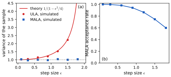
A Gaussian well. For \(E(x)=\frac a2x^2\) the update is the autoregression \(x'=\rho x+\epsilon z\) with \(\rho=1-\frac{\epsilon^2a}{2}\). It has a stationary law iff \(|\rho|<1\), i.e. iff \(\epsilon^2a<4\), and then the stationary variance \(v\) solves \(v=\rho^2v+\epsilon^2\): \[ v=\frac{\epsilon^2}{1-\rho^2}=\frac{\epsilon^2}{\frac{\epsilon^2a}{2}\big(2-\frac{\epsilon^2a}{2}\big)}=\frac{1}{a\,(1-\epsilon^2a/4)}. \] The target variance is \(1/a\), so the relative bias is \(\epsilon^2a/4+O(\epsilon^4)\) and it blows up as \(\epsilon^2a\to4\). With \(a=1\): \(v=1.0230,\,1.099,\,1.333,\,2.286,\,5.263\) for \(\epsilon=0.3,\,0.6,\,1,\,1.5,\,1.8\). Simulation with 4 000 chains and 300 steps gives 2.23 (theory 2.29) at \(\epsilon=1.5\) and 5.02 (theory 5.26) at \(\epsilon=1.8\), and the demonstration agrees within Monte Carlo error. For \(\epsilon^2a>4\) the chain diverges geometrically.
General energies. Near a minimum the energy is approximately quadratic with curvature matrix \(\nabla^2E\); the chain is stable for step sizes satisfying \(\epsilon^2\lambda_{\max}(\nabla^2E)<4\), the same condition as for gradient descent with step \(\epsilon^2/2\). Expert A of Figure 24.1 has wells of variance \(0.45^2\), curvature \(\approx4.9\), so the unadjusted chain is stable only for \(\epsilon<0.9\); at \(\epsilon=1\) it diverges (demonstration, preset 5). The Metropolis step rejects exactly the proposals that would have blown up, so MALA at \(\epsilon=1\) stays stable but accepts only about a quarter of its proposals (preset 6). For the standard Gaussian target MALA's acceptance rate is 0.75 at \(\epsilon=1.5\) and 0.60 at \(\epsilon=1.8\), and its sample variance stays at \(1.00\pm0.03\) while the unadjusted chain's reaches 5.
See also: Section 12.5.6 (Langevin and MALA) and the HMC demonstration with one leapfrog step.
24.2.2 Contrastive divergence
p. 852 Running MCMC to convergence at every gradient step is too expensive. Contrastive divergence (CD; Hinton 2002) starts the chain at a data point and runs it for a fixed small number \(T\) of steps. The book states that \(T\) steps of CD minimise \[ \mathrm{CD}_T=\Dkl(p_0\|p_\infty)-\Dkl(p_T\|p_\infty) \tag{24.19} \] where \(p_T\) is the distribution of the state after \(T\) MCMC updates, \(p_0=p_{\mathcal D}\) and \(p_\infty=p_{\bm\theta}\), and that \(T=1\) often suffices. Gap 24.5 proves what is true about (24.19), and what is only approximately true of the CD update.
24.2.2.1 Fitting RBMs with CD
pp. 853–854 CD was invented for the restricted Boltzmann machine (Section 4.3.3.2), a latent-variable EBM with binary visible units \(\bm x\) and hidden units \(\bm z\) joined by a bipartite graph. I write the energy as a log-linear model with one feature per edge, \[ E(\bm x,\bm z;\bm\theta)=-\sum_{d=1}^D\sum_{k=1}^Kx_dz_kW_{dk}-\sum_dx_db_d-\sum_kz_kc_k \tag{24.20} \] (the book prints the three sums with a plus sign; with \(p\propto e^{-E}\) that sign is inconsistent with (24.21) and the "log-linear" description, see the notes on the book). The unary terms \(b,c\) are weights on units clamped to 1 and are dropped from now on. Since \(p(\bm z\given\bm x)\) and \(p(\bm x\given\bm z)\) both factorise into sigmoids (gap 4.11), block Gibbs sampling is exact and fast, and the log-likelihood gradient is the difference of a clamped and an unclamped expectation (gap 4.19): \[ \frac{\partial\ell}{\partial w_{dk}}=\frac1N\sum_{n=1}^N\E[x_dz_k\given\bm x_n,\bm\theta]-\E[x_dz_k\given\bm\theta] \tag{24.21} \] \[ \nabla_{\bm W}\ell=\E_{p_{\mathcal D}(\bm x)p(\bm z\given\bm x,\bm\theta)}[\bm x\bm z^\T]-\E_{p(\bm z,\bm x\given\bm\theta)}[\bm x\bm z^\T]. \tag{24.22} \] When the two expectations match, the gradient vanishes and learning stops. The first term is a "Hebbian" and the second an "anti-Hebbian" term (cells that fire together wire together). CD-1 approximates the second expectation by one Gibbs sweep started at the data: \[ \bm z_n\sim p(\bm z\given\bm x_n,\bm\theta),\qquad\bm x_n'\sim p(\bm x\given\bm z_n,\bm\theta),\qquad\bm z_n'\sim p(\bm z\given\bm x_n',\bm\theta) \] these are Equations (24.23) to (24.25), and \[ \E_{p(\cdot\given\bm\theta)}[\bm x\bm z^\T]\approx\bm x_n(\bm z_n')^\T \tag{24.26} \] where \(\bm x_n'\) is the model's attempt to reconstruct \(\bm x_n\) after encoding and decoding ("fantasy data"). The variance of the estimate is reduced by using \(\E[\bm z\given\bm x_n']\) in place of the sampled \(\bm z_n'\), whereas replacing the sampled \(\bm z_n\) in (24.23) by its mean is not valid: each hidden unit could then pass more than one bit about \(\bm x_n\) to the reconstruction and would no longer act as a bottleneck.
Algorithm 24.1: CD-1 training for an RBM with binary hidden and visible units
- Initialise \(\bm W\in\R^{D\times K}\) randomly.
- For \(t=1,2,\dots\) and for each minibatch of size \(B\): set \(\bm g:=\bm0\).
- For each case \(\bm x_n\) in the minibatch: compute \(\bm\mu_n=\E[\bm z\given\bm x_n,\bm W]\); sample \(\bm z_n\sim p(\bm z\given\bm x_n,\bm W)\); sample \(\bm x_n'\sim p(\bm x\given\bm z_n,\bm W)\); compute \(\bm\mu_n'=\E[\bm z\given\bm x_n',\bm W]\); accumulate \(\bm g:=\bm g+\bm x_n\bm\mu_n^\T-\bm x_n'(\bm\mu_n')^\T\).
- Update \(\bm W:=\bm W+\eta_t\,\frac1B\bm g\).
Filling the gap 24.4: the expected CD-1 update, reversibility of the Gibbs sweep, and why the sign of (24.20) matters pp. 853–854, (24.20)–(24.26), Algorithm 24.1
Proof
The two expectations. The conditionals and the clamped-minus-unclamped form of the gradient are proved in gap 4.11 and gap 4.19; with the energy (24.20) the sign is such that \(\partial\ell/\partial W_{dk}=\E_{\mathcal D}\E_{z\given x}[x_dz_k]-\E_{p_{\bm\theta}}[x_dz_k]\). (With \(E=+\sum xzW\) the roles of the two terms would be exchanged.) The clamped expectation needs no sampling: since \(z_k\) is conditionally Bernoulli, \(\E[x_dz_k\given\bm x]=x_d\mu_k(\bm x)\) with \(\mu_k(\bm x)=\sigm(c_k+\sum_dW_{dk}x_d)\).
The Gibbs sweep is a reversible kernel with invariant law \(p(\bm x)\). The sweep \(\bm x\to\bm z\to\bm x'\) has transition probability \(K(\bm x,\bm x')=\sum_{\bm z}p(\bm z\given\bm x)p(\bm x'\given\bm z)\). Then \[ p(\bm x)K(\bm x,\bm x')=\sum_{\bm z}p(\bm x,\bm z)\frac{p(\bm x',\bm z)}{p(\bm z)}, \] which is symmetric in \((\bm x,\bm x')\): detailed balance holds, so \(p\) is invariant. (This is exactly the kernel of the enumerable RBM in Figure 24.x2, and invariance and reversibility were confirmed to \(10^{-13}\).)
The expected update. Let \(p_1=p_{\mathcal D}K\) be the law of \(\bm x_n'\) when \(\bm x_n\sim p_{\mathcal D}\). The one-sample update of Algorithm 24.1 has mean \[ \E[\Delta\bm W]=\E_{p_{\mathcal D}}\big[\bm x\bm\mu(\bm x)^\T\big]-\E_{p_1}\big[\bm x\bm\mu(\bm x)^\T\big], \] because \(\E[\bm z_n'\given\bm x_n']=\bm\mu(\bm x_n')\): replacing \(\bm z_n'\) by \(\bm\mu_n'\) is a Rao–Blackwellisation, which leaves the mean unchanged and cannot increase the variance (law of total variance). This expected update, with no sampling noise, is what the demonstration and Figure 24.x2 use; \(k\) sweeps replace \(p_1\) by \(p_{\mathcal D}K^k\). The exact gradient is the same expression with \(p_1\) replaced by \(p_{\bm\theta}\), so \[ \text{(exact gradient)}-\E[\Delta\bm W]=\E_{p_1}[\bm x\bm\mu^\T]-\E_{p_{\bm\theta}}[\bm x\bm\mu^\T], \] the difference of one statistic under \(p_1\) and under the model: the CD-1 bias is exactly the failure of one sweep to reach \(p_{\bm\theta}\).
Why \(\bm z_n\) must be sampled. The reconstruction \(\bm x_n'\sim p(\bm x\given\bm z_n)\) with \(\bm z_n\in\{0,1\}^K\) is one step of the reversible kernel above. If \(\bm z_n\) is replaced by \(\bm\mu_n\in[0,1]^K\) the reconstruction distribution is \(p(\bm x\given\bm z=\bm\mu_n)\), which is not a state of the chain: it lets the hidden layer carry \(K\) real numbers (not \(K\) bits) about \(\bm x_n\), the reconstruction looks too much like \(\bm x_n\), and \(\bm x_n'\) is no longer a sample from \(p_{\mathcal D}K\). The error is a bias of the negative phase toward the data.
Filling the gap 24.5: what CD optimises (24.19): it is non-negative and monotone, equals an expected KL, and is biased p. 852, (24.19), and the bias remarks on p. 855
Proof
Setting. Let \(K\) be a Markov kernel with invariant distribution \(p_\infty\) (for CD, a Gibbs or Langevin sweep for the current \(\bm\theta\)), and \(p_T=p_0K^T\). I write the proofs for a finite state space; the continuous case is identical with sums replaced by integrals.
Data processing for a kernel that fixes \(p_\infty\). Let \(r(x\given y)=p_\infty(x)K(x,y)/p_\infty(y)\) be the time-reversed kernel and \(\tilde p(x\given y)=p(x)K(x,y)/(pK)(y)\) the posterior of the previous state given that \(p\) moved to \(y\). The joint laws \(p\otimes K\) of \((x,y)\) and \(p_\infty\otimes K\) have KL divergence \(\Dkl(p\|p_\infty)\) (the kernel is common), and the chain rule in the other order gives \[ \Dkl(p\|p_\infty)=\Dkl(pK\|p_\infty)+\E_{y\sim pK}\big[\Dkl(\tilde p(\cdot\given y)\|r(\cdot\given y))\big]. \] Hence \(\Dkl(pK\|p_\infty)\le\Dkl(p\|p_\infty)\) with equality iff \(\tilde p=r\) for every \(y\) in the support, i.e. \(p(x)/p_\infty(x)=(pK)(y)/p_\infty(y)\) whenever \(K(x,y)>0\). If all entries of \(K\) are positive (as for the Gibbs sweep of an RBM), this forces \(p/p_\infty\) to be constant, i.e. \(p=p_\infty\).
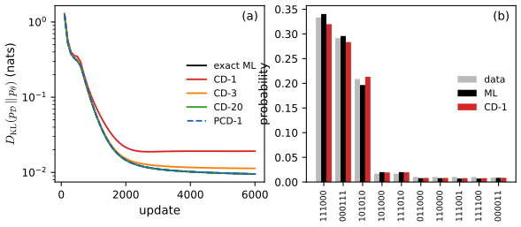
Consequences for (24.19). (a) \(\Dkl(p_T\|p_\infty)\) is non-increasing in \(T\), so \(\mathrm{CD}_T\) is non-negative and non-decreasing in \(T\) and bounded by \(\Dkl(p_0\|p_\infty)\). (b) \(\mathrm{CD}_1=\E_{y\sim p_1}\Dkl(\tilde p(\cdot\given y)\|r(\cdot\given y))\) is an expected KL between the posterior of the data point behind a reconstruction and the model's reversed chain: it is zero iff one sweep does not move the data distribution's KL at all, and (for a positive kernel) iff \(p_0=p_\infty\). (c) If \(K\) is ergodic, \(\Dkl(p_T\|p_\infty)\to0\), so \(\mathrm{CD}_T\to\Dkl(p_0\|p_\infty)\): CD tends to maximum likelihood as \(T\to\infty\). On the RBM of Figure 24.x2 (random weights, random data law) \(\mathrm{CD}_T\) rises from 3.503 nats at \(T=1\) to 4.273 at \(T=40\), is non-decreasing at every step, and \(\mathrm{CD}_1\) equals the expected KL in (b) to \(10^{-10}\).
What the CD update is, and is not. Write \(-\mathrm{CD}_T\) as \(-\Dkl(p_0\|p_{\bm\theta})+\Dkl(p_T\|p_{\bm\theta})\). The first part has gradient \(\nabla_{\bm\theta}\ell=-\E_{p_0}[\nabla_{\bm\theta}E]+\E_{p_{\bm\theta}}[\nabla_{\bm\theta}E]\) (gap 24.2). The CD update is obtained by dropping the dependence of \(p_T\) on \(\bm\theta\) inside the second part, which then contributes \(-\E_{p_T}[\nabla_{\bm\theta}\log p_{\bm\theta}]\), and the sum is \[ \Delta\bm\theta_{\mathrm{CD}_T}=-\E_{p_0}[\nabla_{\bm\theta}E_{\bm\theta}]+\E_{p_T}[\nabla_{\bm\theta}E_{\bm\theta}]. \] This is not the gradient of \(\mathrm{CD}_T\) (the dropped term does not vanish, and the update need not be the gradient of any function), which is why the book speaks of the update only approximately minimising (24.19).
The bias. The difference to the exact gradient is \((\E_{p_T}-\E_{p_{\bm\theta}})[\nabla_{\bm\theta}E]\), bounded by \(2\sup\|\nabla_{\bm\theta}E\|\cdot\mathrm{TV}(p_T,p_{\bm\theta})\), and for a finite ergodic reversible chain \(\mathrm{TV}(p_T,p_\infty)\le C|\lambda_2|^T\) with \(\lambda_2\) the second-largest eigenvalue modulus: the bias decays geometrically in \(T\). On the example RBM the norm of the difference falls as \(0.70,\,0.23,\,0.021,\,1.8\times10^{-4},\,1.2\times10^{-8}\) for \(T=1,2,4,8,16\) (and to rounding error afterwards). Because the bias is zero only if \(p_T\) matches the model statistic, the maximum-likelihood optimum is not a fixed point of CD-1: at the end of the exact-ML run of Figure 24.x2 the CD-1 update has size 0.0027, whereas at the end of the CD-1 run the exact likelihood gradient has size 0.018. CD-1 therefore converges to a different point (final KL 0.0192 against 0.0095), as in the figure. The extra Gibbs steps of CD-\(k\) shrink the bias as above: 0.0113 for \(k=3\) and 0.0095 for \(k=20\).
See also: Section 12.2 (Metropolis–Hastings) and gap 5.7 (the chain rule for KL).
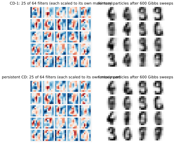
pp. 853–854 Figure 24.2 of the book is a schematic of the chain \(\bm x\to\bm z\to\bm x'\to\cdots\) (it is not reproduced). To see CD on real data, Figure 24.x3 trains the RBM of Algorithm 24.1 on the 8 × 8 digits that ship with scikit-learn (64 visible units, 64 hidden units, pixel intensity/16 used as the probability that a visible unit is on; 80 epochs, minibatch 50, learning rate 0.05), once with CD-1 and once with persistent chains (next subsection). The fantasy particles are what the model dreams after 600 sweeps of block Gibbs sampling from random starts.
24.2.2.2 Persistent CD
pp. 854–855 Persistent CD (PCD; Younes 1999, Tieleman 2008) does not restart the chain at the data: it keeps \(S\) chains and, after each parameter update, continues them from where they were for a few steps. Two dynamics run at different time scales, the states quickly and the parameters slowly. Younes's justification is that \(p(\bm x\given\bm\theta_t)\) is close to \(p(\bm x\given\bm\theta_{t-1})\) because the parameters moved only a little, so a few steps from the old state suffice.
Algorithm 24.2: persistent MCMC-SGD for fitting an EBM (corrected)
- Initialise \(\bm\theta\) randomly, chains \(\tilde{\bm x}_{1:S}\) randomly, and the learning rate \(\eta\).
- For \(t=1,2,\dots\) and each minibatch of size \(B\): \(\bm g_b=\nabla_{\bm\theta}E_{\bm\theta}(\bm x_b)\) for the data points \(\bm x_b\).
- For \(s=1,\dots,S\): advance the chain, \(\tilde{\bm x}_s\sim\mathrm{MCMC}(\text{target}=p(\cdot\given\bm\theta),\ \text{init}=\tilde{\bm x}_s,\ N\text{ steps})\); set \(\tilde{\bm g}_s=\nabla_{\bm\theta}E_{\bm\theta}(\tilde{\bm x}_s)\).
- \(\bm g_t=-\frac1B\sum_b\bm g_b+\frac1S\sum_s\tilde{\bm g}_s\); update \(\bm\theta:=\bm\theta+\eta\bm g_t\); decrease \(\eta\).
The book's line 10 is \(\bm g_t=-\frac1B\sum_b\bm g_b-\frac1S\sum_s\tilde{\bm g}_s\); the model term must enter with the opposite sign of the data term, as (24.7) and gap 24.2 show (gap 24.6). The book also refers to this pseudocode as "Algorithm 12"; it is Algorithm 24.2.
Filling the gap 24.6: persistent chains track the model, their fixed points are the likelihood optima, and the sign of Algorithm 24.2 pp. 854–855, Algorithm 24.2
Proof
Sign. Ascent on \(\ell\) uses \(\nabla_{\bm\theta}\ell=-\E_{p_{\mathcal D}}[\nabla_{\bm\theta}E]+\E_{p_{\bm\theta}}[\nabla_{\bm\theta}E]\) (24.7, 24.15): the sample average of the model energy gradient is added, the data average subtracted. With both terms negative, as printed, there is no stationary point at all. For \(E=\frac a2x^2\) and \(N(0,1)\) data the correct update is \(-\frac12+\frac1{2a}\), zero exactly at the right precision \(a=1\), while the printed one is \(-\frac12-\frac1{2a}<0\) for every \(a>0\), so the update never stops pushing \(a\) downwards, towards a non-normalisable energy (both facts checked numerically).
Tracking. Let \(K_{\bm\theta}\) be the chain's kernel with invariant law \(p_{\bm\theta}\), assume it contracts in total variation: \(\|\mu K_{\bm\theta}-\nu K_{\bm\theta}\|_{\mathrm{TV}}\le\lambda\|\mu-\nu\|_{\mathrm{TV}}\) with \(\lambda<1\) uniformly (a Doeblin condition), that \(\bm\theta\mapsto p_{\bm\theta}\) is \(L\)-Lipschitz in TV, and that each parameter step has size at most \(\eta G\) (learning rate times a gradient bound). The persistent distribution \(q_t=q_{t-1}K_{\bm\theta_t}\) obeys, since \(p_{\bm\theta_t}K_{\bm\theta_t}=p_{\bm\theta_t}\), \[ \|q_t-p_{\bm\theta_t}\|_{\mathrm{TV}}=\|(q_{t-1}-p_{\bm\theta_t})K_{\bm\theta_t}\|_{\mathrm{TV}}\le\lambda\big(\|q_{t-1}-p_{\bm\theta_{t-1}}\|_{\mathrm{TV}}+L\eta G\big), \] so the tracking error \(e_t\) satisfies \(\limsup e_t\le\lambda L\eta G/(1-\lambda)=O(\eta)\): the persistent chain stays within \(O(\eta)\) of the current model, and the error vanishes when the learning rate is decreased (line 12). CD has no such guarantee, because its chain is restarted from the data at every step.
Fixed points. If the joint dynamics of \((\bm\theta,q)\) rest, then \(q=qK_{\bm\theta}\), so \(q=p_{\bm\theta}\) for an ergodic kernel, and the update vanishes iff \(\E_{p_{\mathcal D}}[\nabla E]=\E_{q}[\nabla E]=\E_{p_{\bm\theta}}[\nabla E]\), i.e. iff \(\nabla_{\bm\theta}\ell=0\) (gap 24.2): the fixed points of persistent CD are exactly the stationary points of the likelihood, in contrast to CD-\(T\) (gap 24.5). On the enumerable RBM of Figure 24.x2 the final likelihood gradient of the PCD run is below \(5\times10^{-3}\) and its final KL equals that of exact maximum likelihood to four digits. Slow mixing remains the practical limit: if the chains cannot cross between modes at the speed the model changes, \(\lambda\) is close to 1 and the bound is useless (the replay buffers mentioned next address this).
24.2.2.3 Other methods
p. 855 PCD can be improved by keeping a replay buffer of historical chain states and starting new chains from random buffer entries (Du and Mordatch 2019). Other variants are mean-field CD and multigrid CD. Because truncated MCMC gives biased gradients (gap 24.5), several lines of work remove the bias: unbiased gradient estimators from coupled chains, and differentiating through the sampler with an entropy correction (Du et al. 2020).
24.3 Score matching (SM)
pp. 855–856 If two continuously differentiable functions have equal first derivatives everywhere, they differ by a constant; for two log-densities the normalisation then forces the constant to be zero. So one can fit an EBM by matching the first derivatives of its log-density to those of the data. The gradient of a log-density with respect to its input is the (Stein) score (not to be confused with the Fisher score \(\nabla_{\bm\theta}\log p\)); for an EBM it is free of \(Z_{\bm\theta}\): \[ \sc_{\bm\theta}(\bm x)\triangleq\nabla_{\bm x}\log p_{\bm\theta}(\bm x)=-\nabla_{\bm x}E_{\bm\theta}(\bm x). \tag{24.27} \] Score matching (Hyvärinen 2005) minimises the Fisher divergence \[ \DF(p_{\mathcal D}\|p_{\bm\theta})=\E_{p_{\mathcal D}(\bm x)}\Big[\tfrac12\|\nabla_{\bm x}\log p_{\mathcal D}(\bm x)-\nabla_{\bm x}\log p_{\bm\theta}(\bm x)\|^2\Big] \tag{24.28} \] whose expectation is estimated by a sample mean. The obstacle is the data score \(\nabla\log p_{\mathcal D}\), which is unknown.
24.3.1 Basic score matching
p. 856 Hyvärinen showed that under regularity conditions an integration by parts replaces the unknown data score by second derivatives of the energy: \[ \DF(p_{\mathcal D}\|p_{\bm\theta})=\E_{p_{\mathcal D}}\Big[\frac12\sum_{i=1}^d\Big(\frac{\partial E_{\bm\theta}}{\partial x_i}\Big)^2-\frac{\partial^2E_{\bm\theta}}{\partial x_i^2}\Big]+\const \tag{24.29} \] \[ =\E_{p_{\mathcal D}}\Big[\tfrac12\|\sc_{\bm\theta}(\bm x)\|^2+\tr\big(\bm J_{\bm x}\sc_{\bm\theta}(\bm x)\big)\Big]+\const \tag{24.30} \] with \(\bm J_{\bm x}\sc_{\bm\theta}\) the Jacobian of the score. The estimator is consistent under regularity conditions. Its cost is the trace of the Jacobian, \(O(d^2)\) for a network (one backward pass per coordinate), so the implicit form was used only for simple energies.
Filling the gap 24.7: equal scores imply equal densities (and when not), the integration by parts, consistency, and the closed form for energies linear in their parameters pp. 855–856, (24.27)–(24.30)
Proof
Equal scores. If \(\nabla\log p=\nabla\log q\) on a connected open set \(\Omega\) where both densities are positive, then \(\log p-\log q\) has zero gradient on \(\Omega\), hence is constant there, and if \(\Omega\) carries all the mass, \(\int p=\int q=1\) forces the constant to be 0. The qualifier is real: if the support is disconnected (or the density is nearly zero between modes), the score does not see the relative weights of the components. For \(p_w=w\,p_1+(1-w)\,p_2\) with essentially disjoint supports, \(\nabla\log p_w=\nabla\log p_1\) on the first and \(\nabla\log p_2\) on the second, whatever \(w\) is: score matching identifies the shapes of the modes but only weakly their mixing proportions. (The demonstration's mixtures have modes overlapping enough for this to be a mild effect.)
Integration by parts. Expand (24.28): \(\DF=\frac12\E\|\sc_{\mathcal D}\|^2-\E[\sc_{\mathcal D}^\T\sc_{\bm\theta}]+\frac12\E\|\sc_{\bm\theta}\|^2\), all expectations under \(p_{\mathcal D}\). The middle term is the only one involving the unknown score, and \(p_{\mathcal D}\sc_{\mathcal D}=\nabla p_{\mathcal D}\), so \[ \E_{p_{\mathcal D}}[\sc_{\mathcal D}^\T\sc_{\bm\theta}]=\int\nabla p_{\mathcal D}(\bm x)^\T\sc_{\bm\theta}(\bm x)\,\d\bm x=-\int p_{\mathcal D}(\bm x)\,\nabla\!\cdot\!\sc_{\bm\theta}(\bm x)\,\d\bm x=-\E_{p_{\mathcal D}}\big[\tr\bm J_{\bm x}\sc_{\bm\theta}\big]. \] The second equality is the divergence theorem on a ball \(B_R\) with the surface term \(\oint_{\partial B_R}p_{\mathcal D}\,\sc_{\bm\theta}\cdot\bm n\,\d S\), which tends to zero as \(R\to\infty\) provided \(p_{\mathcal D}\sc_{\bm\theta}\to0\) fast enough at infinity; the conditions are that \(p_{\mathcal D}\) is differentiable, \(\E\|\sc_{\mathcal D}\|^2\) and \(\E\|\sc_{\bm\theta}\|^2\) are finite, and the boundary term vanishes. Substituting gives (24.30), and with \(\sc_{\bm\theta}=-\nabla E_{\bm\theta}\), \(\tr\bm J_{\bm x}\sc_{\bm\theta}=-\sum_i\partial_i^2E_{\bm\theta}\), (24.29). The constant is \(\frac12\E\|\sc_{\mathcal D}\|^2\). On the bimodal sample of the demonstration, the explicit and implicit objectives differ by the same number, 1.2244, for four different parameter vectors (spread \(4\times10^{-11}\)), and that number equals \(\frac12\E\|\sc_{\mathcal D}\|^2\).
Consistency. If \(p_{\mathcal D}=p_{\bm\theta^*}\) then \(\DF=0\) at \(\bm\theta^*\), the population minimum, and \(\DF(\bm\theta)=0\) forces \(\sc_{\bm\theta}=\sc_{\bm\theta^*}\) a.e., hence (connected support) \(p_{\bm\theta}=p_{\bm\theta^*}\); with identifiability of \(\bm\theta\) in the model the population minimiser is unique. The sample objective converges uniformly to the population one under standard moment conditions, so its minimiser converges to \(\bm\theta^*\) (the argument for any M-estimator; Hyvärinen 2005). Numerically, 300 000 draws from a quartic exponential family return the parameters within 0.012.
Closed form. Let \(E_{\bm\theta}(\bm x)=\bm\theta^\T\bm\phi(\bm x)\), with \(\bm\phi:\R^d\to\R^m\) and Jacobian \(\bm J_\phi\in\R^{m\times d}\). Then \(\sc_{\bm\theta}=-\bm J_\phi^\T\bm\theta\) and \(\tr\bm J_{\bm x}\sc_{\bm\theta}=-\bm\theta^\T\Delta\bm\phi\) (\(\Delta\) the Laplacian applied coordinatewise), so (24.30) is the quadratic \[ \tfrac12\bm\theta^\T\bm A\bm\theta-\bm\theta^\T\bm b,\qquad\bm A=\E_{p_{\mathcal D}}[\bm J_\phi\bm J_\phi^\T],\quad\bm b=\E_{p_{\mathcal D}}[\Delta\bm\phi], \] minimised by \(\hat{\bm\theta}=\bm A^{-1}\bm b\) when \(\bm A\succ0\): score matching is a single linear solve, with no sampling, no \(Z_{\bm\theta}\) and no iteration. (Contrast maximum likelihood for the same family, a convex problem needing a model expectation at each Newton step, gap 24.2.) In 1-D with \(\bm\phi=(x,x^2,x^3,x^4)\) the matrix is \(4\times4\) and this is the fit used in the demonstration; a BFGS minimisation of the implicit objective returns the same \(\hat{\bm\theta}\) (difference \(2\times10^{-7}\)). For the Gaussian family \(E=\frac12(\bm x-\bm\mu)^\T\bm\Lambda(\bm x-\bm\mu)\) the empirical objective is \(\frac12\tr(\bm\Lambda\bm S\bm\Lambda)-\tr\bm\Lambda\) at \(\bm\mu=\bar{\bm x}\) (the minimum over \(\bm\mu\), as \(\E\|\bm\Lambda(\bm x-\bm\mu)\|^2\) is smallest at the mean), whose gradient \(\bm\Lambda\bm S-\bm I=\bm0\) gives \(\hat{\bm\Lambda}=\bm S^{-1}\): score matching reproduces the maximum-likelihood estimate for a Gaussian (confirmed: variance 2.9675 by both). For a non-Gaussian misspecified family the two differ: on the 400-point bimodal sample the quartic energy fitted by SM has \(\Dkl\) 0.066 to the truth against 0.053 for maximum likelihood.
24.3.2 Denoising score matching (DSM)
pp. 857–858 Score matching needs \(\log p_{\mathcal D}\) to be differentiable and finite everywhere. A distribution of images with pixel values in \(\{0,\dots,255\}\) is discrete and bounded: \(\log p_{\mathcal D}\) is discontinuous and \(-\infty\) outside the range. The remedy is to add smooth noise, \(\tilde{\bm x}=\bm x+\bm\epsilon\); the noisy law \(q(\tilde{\bm x})=\int q(\tilde{\bm x}\given\bm x)p_{\mathcal D}(\bm x)\d\bm x\) is smooth, and Vincent (2011) showed \[ \DF(q(\tilde{\bm x})\|p_{\bm\theta}(\tilde{\bm x}))=\E_{q(\tilde{\bm x})}\big[\tfrac12\|\nabla_{\tilde{\bm x}}\log p_{\bm\theta}(\tilde{\bm x})-\nabla_{\tilde{\bm x}}\log q(\tilde{\bm x})\|^2\big] \tag{24.31} \] \[ =\E_{q(\bm x,\tilde{\bm x})}\big[\tfrac12\|\nabla_{\tilde{\bm x}}\log p_{\bm\theta}(\tilde{\bm x})-\nabla_{\tilde{\bm x}}\log q(\tilde{\bm x}\given\bm x)\|^2\big] \tag{24.32} \] \[ =\tfrac12\E_{q(\bm x,\tilde{\bm x})}\Big[\Big\|\sc_{\bm\theta}(\tilde{\bm x})-\frac{\bm x-\tilde{\bm x}}{\sigma^2}\Big\|^2\Big]+\const \tag{24.33} \] the last line for \(q(\tilde{\bm x}\given\bm x)=\N(\tilde{\bm x};\bm x,\sigma^2\bm I)\), where \[ \nabla_{\tilde{\bm x}}\log q(\tilde{\bm x}\given\bm x)=-\frac{\tilde{\bm x}-\bm x}{\sigma^2}. \tag{24.34} \] The target \((\bm x-\tilde{\bm x})/\sigma^2\) points from the noisy sample to the clean one, so the score network is trained to denoise (this returns in Section 25.3 for diffusion models). The tie to Tweedie's formula and Stein's unbiased risk estimate is noted below.
Filling the gap 24.8: Vincent's identity, Tweedie's formula, the bias of DSM, and the variance as \(\sigma\to0\) pp. 857–858, (24.31)–(24.36)
Proof
The identity. Expand (24.31): \(\DF(q\|p_{\bm\theta})=\E_q[\frac12\|\sc_{\bm\theta}\|^2]-\E_q[\sc_q^\T\sc_{\bm\theta}]+\frac12\E_q\|\sc_q\|^2\). The cross term is where the unknown \(q\) appears, but \(q(\tilde{\bm x})\sc_q(\tilde{\bm x})=\nabla q(\tilde{\bm x})=\int p_{\mathcal D}(\bm x)\nabla_{\tilde{\bm x}}q(\tilde{\bm x}\given\bm x)\d\bm x=\int p_{\mathcal D}(\bm x)q(\tilde{\bm x}\given\bm x)\nabla_{\tilde{\bm x}}\log q(\tilde{\bm x}\given\bm x)\d\bm x\), hence \[ \E_q[\sc_q^\T\sc_{\bm\theta}]=\E_{q(\bm x,\tilde{\bm x})}\big[\nabla_{\tilde{\bm x}}\log q(\tilde{\bm x}\given\bm x)^\T\sc_{\bm\theta}(\tilde{\bm x})\big]. \] Completing the square in this joint expectation gives \[ \DF(q\|p_{\bm\theta})=\E_{q(\bm x,\tilde{\bm x})}\big[\tfrac12\|\sc_{\bm\theta}-\nabla\log q(\tilde{\bm x}\given\bm x)\|^2\big]-\underbrace{\tfrac12\E_{q(\bm x,\tilde{\bm x})}\|\nabla\log q(\tilde{\bm x}\given\bm x)\|^2+\tfrac12\E_q\|\sc_q\|^2}_{C,\ \text{free of }\bm\theta}, \] which is (24.32), and for the Gaussian kernel \(\nabla\log q(\tilde{\bm x}\given\bm x)=-\bm z/\sigma\) with \(\bm z=(\tilde{\bm x}-\bm x)/\sigma\), whence \(\tfrac12\E\|\cdot\|^2=d/(2\sigma^2)\) and (24.33). Nothing about \(p_{\mathcal D}\) is needed: not differentiability, not even a density (the empirical distribution of the sample works). Numerically (quadrature on a bimodal \(p_{\mathcal D}\) with \(\sigma=0.5\), three quartic energies) the difference between the left side and the DSM expectation is the same constant to \(3\times10^{-5}\).
Tweedie. The minimiser of (24.33) over all functions is the conditional mean \(\sc^*(\tilde{\bm x})=\E[(\bm x-\tilde{\bm x})/\sigma^2\given\tilde{\bm x}]\); but it is also \(\sc_q=\nabla\log q\) by the identity above. Equating, \[ \E[\bm x\given\tilde{\bm x}]=\tilde{\bm x}+\sigma^2\nabla_{\tilde{\bm x}}\log q(\tilde{\bm x}), \] Tweedie's formula for Gaussian noise (gap 3.39): a denoiser and a score are the same object up to the factor \(\sigma^2\) (checked on the bimodal mixture at three points to \(10^{-4}\)).
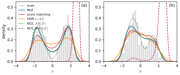
Bias. The DSM population minimiser is the score of the noisy law \(q\), so a well-specified EBM fitted by DSM recovers \(q=p_{\mathcal D}*\N(\bm0,\sigma^2\bm I)\), not \(p_{\mathcal D}\): \(\DF(q\|p_{\bm\theta})\ne\DF(p_{\mathcal D}\|p_{\bm\theta})\) in general. For \(p_{\mathcal D}=\N(0,s^2)\) and \(E=\frac a2x^2\), \(q=\N(0,s^2+\sigma^2)\) and the optimum is \[ a^*=\frac1{s^2+\sigma^2}\quad\text{(true value }1/s^2\text{)}: \] with \(s=1\), \(\sigma=0.3\) the fitted precision is 0.917 (simulation: 0.9168), a variance inflated by 9%; with \(\sigma=1\) it is 0.5, a variance twice the truth (simulation 0.4996). The bimodal quartic fit shows the same thing: \(\Dkl\) to the truth rises from 0.053 (MLE) to 0.070, 0.132 and 0.288 for \(\sigma=0.2,0.5,1\) (Figure 24.x4, demonstration preset 3).
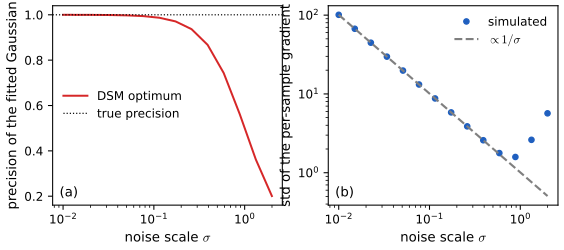
Variance. Take \(\sigma\to0\) with the Gaussian family above. The per-sample gradient of the DSM loss \(\frac12(-a\tilde x+z/\sigma)^2\) in \(a\) is \(a\tilde x^2-z\tilde x/\sigma=a\tilde x^2-zx/\sigma-z^2\), whose dominant random part \(zx/\sigma\) has standard deviation \(s/\sigma\): it grows like \(1/\sigma\) (simulated slope of \(\log\) std against \(\log\sigma\): \(-1.000\); std 100.9, 10.1, 1.74 for \(\sigma=0.01,0.1,1\)). In general, expanding \(\sc_{\bm\theta}(\bm x+\sigma\bm z)=\sc_{\bm\theta}(\bm x)+\sigma\bm J\bm z+O(\sigma^2)\) in (24.35) gives \(\frac{\|\bm z\|^2}{2\sigma^2}+\frac{\bm z^\T\sc_{\bm\theta}(\bm x)}{\sigma}+O(1)\): the first term does not depend on \(\bm\theta\) (it inflates the variance of the loss value but not of its gradient) and the second does (the printed (24.36) writes "+constant" for the \(O(1)\) rest, which is \(\bm\theta\)-dependent but bounded; the leftover mean square stays at 7.9 as \(\sigma\) goes from 0.01 to 0.001 in a numerical test). The gradient variance \(\E\|\nabla_{\bm\theta}\sc_{\bm\theta}^\T\bm z\|^2/\sigma^2\) therefore grows like \(\sigma^{-2}\), the trade-off the book describes: small \(\sigma\) reduces the bias \(O(\sigma^2)\) and inflates the variance. A simple remedy is antithetic noise: evaluate the loss at \(\tilde{\bm x}_\pm=\bm x\pm\sigma\bm z\) and average; the \(1/\sigma\) terms cancel exactly (\(\bm z^\T\sc(\bm x)/\sigma\) changes sign) and the pair's gradient standard deviation stays at 2.0 for both \(\sigma=0.01\) and \(\sigma=0.1\), against 100.9 without pairing.
24.3.3 Sliced score matching (SSM)
pp. 858–859 DSM avoids second derivatives but fits the noisy law, not \(p_{\mathcal D}\). Sliced score matching (Song et al. 2019) keeps consistency and cost \(O(d)\): it projects both scores on a random direction \(\bm v\sim p(\bm v)\) with \(\E[\bm v\bm v^\T]\succ0\) and compares the scalars, \[ \mathrm{D}_{\mathrm{SF}}(p_{\mathcal D}\|p_{\bm\theta})=\E_{p_{\mathcal D}}\E_{p(\bm v)}\big[\tfrac12(\bm v^\T\nabla\log p_{\mathcal D}-\bm v^\T\nabla\log p_{\bm\theta})^2\big]. \tag{24.37} \] By the same integration by parts, with \(\sc_{\bm\theta}=-\nabla E_{\bm\theta}\) (gap 24.9), \[ \mathrm{D}_{\mathrm{SF}}=\E_{p_{\mathcal D}}\E_{p(\bm v)}\Big[\tfrac12\Big(\sum_{i}\frac{\partial E_{\bm\theta}}{\partial x_i}v_i\Big)^2-\sum_{i,j}\frac{\partial^2E_{\bm\theta}}{\partial x_i\partial x_j}v_iv_j\Big]+C. \tag{24.38'} \] The book prints a plus sign before the Hessian term in (24.38) and (24.41); it must be a minus (see the notes on the book). The Hessian term is computed in \(O(d)\) as \[ \sum_{i,j}\frac{\partial^2E}{\partial x_i\partial x_j}v_iv_j=\sum_i\frac{\partial}{\partial x_i}\Big(\underbrace{\sum_j\frac{\partial E}{\partial x_j}v_j}_{f(\bm x)}\Big)v_i \tag{24.39} \] (one gradient to form \(f\), one more reverse-mode pass for \(\nabla f\)), against \(d\) passes for the full trace. For \(p(\bm v)=\N(\bm0,\bm I)\), \(\E_{\bm v}[\frac12(\bm v^\T\nabla E)^2]=\frac12\|\nabla E\|^2\) in closed form (24.40), giving \[ \mathrm{D}_{\mathrm{SF}}=\E\,\E_{\bm v\sim\N(\bm0,\bm I)}\big[\tfrac12(\bm v^\T\sc_{\bm\theta})^2+\bm v^\T\bm J\bm v\big]+C,\qquad\bm J=\bm J_{\bm x}\sc_{\bm\theta}, \tag{24.41, 24.42} \] the Hutchinson (Skilling–Hutchinson) trace estimator applied to (24.30), with \(\bm J\bm v\) a Jacobian–vector product.
Filling the gap 24.9: the sliced objective with its correct sign, the Hessian-vector trick, and the variance of the trace estimators pp. 858–859, (24.37)–(24.42)
Proof
Identifiability. If \(\E[\bm v\bm v^\T]\succ0\) and \(\mathrm D_{\mathrm{SF}}=0\), then \(\E_{p_{\mathcal D}}[\Delta^\T\E[\bm v\bm v^\T]\Delta]=0\) with \(\Delta=\sc_{\mathcal D}-\sc_{\bm\theta}\), so \(\Delta=\bm0\) a.e.; \(\mathrm D_{\mathrm{SF}}\) is a proper divergence, and consistency follows as for (24.28) (gap 24.7).
The implicit form and its sign. Fix \(\bm v\) and expand: \(\frac12(\bm v^\T\sc_{\mathcal D})^2-(\bm v^\T\sc_{\mathcal D})(\bm v^\T\sc_{\bm\theta})+\frac12(\bm v^\T\sc_{\bm\theta})^2\). The cross term: \(\E_{p_{\mathcal D}}[(\bm v^\T\sc_{\mathcal D})(\bm v^\T\sc_{\bm\theta})]=\int(\bm v^\T\nabla p_{\mathcal D})(\bm v^\T\sc_{\bm\theta})\d\bm x=-\int p_{\mathcal D}\,\bm v^\T\nabla(\bm v^\T\sc_{\bm\theta})\d\bm x=-\E_{p_{\mathcal D}}[\bm v^\T\bm J_{\bm x}\sc_{\bm\theta}\,\bm v]\) (the same integration by parts as in gap 24.7, now along \(\bm v\), under the same boundary conditions). So \[ \mathrm D_{\mathrm{SF}}=\E\E_{\bm v}\big[\tfrac12(\bm v^\T\sc_{\bm\theta})^2+\bm v^\T(\bm J_{\bm x}\sc_{\bm\theta})\bm v\big]+C,\qquad C=\tfrac12\E\E_{\bm v}(\bm v^\T\sc_{\mathcal D})^2. \] Now \(\sc_{\bm\theta}=-\nabla E_{\bm\theta}\) and \(\bm J_{\bm x}\sc_{\bm\theta}=-\nabla^2E_{\bm\theta}\), so the second term is \(-\bm v^\T\nabla^2E\,\bm v\), not \(+\), as (24.42) itself shows (it has \(+\bm v^\T\bm J\bm v\) with \(\bm J\) the Jacobian of the score). A closed-form test: for Gaussian data \(\N(\bm0,\bm\Sigma)\) and a Gaussian EBM \(E=\frac12\bm x^\T\bm\Lambda\bm x\) with \(\bm v\sim\N(\bm0,\bm I)\), the explicit divergence is \(\frac12\tr((\bm\Lambda-\bm\Sigma^{-1})\bm\Sigma(\bm\Lambda-\bm\Sigma^{-1}))\), the implicit objective with the minus sign is \(\frac12\tr(\bm\Lambda\bm\Sigma\bm\Lambda)-\tr\bm\Lambda\), and their difference is the constant \(\frac12\tr\bm\Sigma^{-1}\) for every \(\bm\Lambda\); with a plus sign (\(+\tr\bm\Lambda\)) the difference changes with \(\bm\Lambda\), and minimising that objective would not give \(\bm\Lambda=\bm\Sigma^{-1}\) (numerical test with three random \(\bm\Lambda\) in 3-D: spread 5.6 with the plus sign, \(10^{-9}\) with the minus sign).
The Hessian-vector trick (24.39). \(\sum_{i,j}\partial_i\partial_jE\,v_iv_j=\bm v^\T(\nabla^2E)\bm v=\bm v^\T\nabla_{\bm x}(\bm v^\T\nabla_{\bm x}E)\): form the scalar \(f(\bm x)=\bm v^\T\nabla E\) (one backward pass), then differentiate it (a second backward pass) and dot with \(\bm v\). The cost is a small constant multiple of one gradient, independent of \(d\), while \(\tr\nabla^2E\) needs \(d\) such passes. (Checked against the explicit Hessian of a random network: agreement to \(10^{-10}\).)
Gaussian projections recover SM. For \(\E[\bm v\bm v^\T]=\bm I\): \(\E_{\bm v}[(\bm v^\T\sc)^2]=\|\sc\|^2\) and \(\E_{\bm v}[\bm v^\T\bm J\bm v]=\tr\bm J\), so the expected SSM objective equals the SM integrand (24.30): SSM is a stochastic estimator of SM (numerically \(-8.13\) from \(4\times10^5\) Gaussian and \(-8.17\) from Rademacher projections, against \(-8.12\) exactly, for a random 4-D quadratic).
Variance of the trace estimator. For a fixed matrix \(\bm A\) with symmetric part \(\bm A_s\), \(\bm v^\T\bm A\bm v=\bm v^\T\bm A_s\bm v\) has mean \(\tr\bm A\) for \(\E[\bm v\bm v^\T]=\bm I\) and variance \[ \var(\bm v^\T\bm A\bm v)=2\|\bm A_s\|_F^2\ \ (\bm v\sim\N(\bm0,\bm I)),\qquad 2\Big(\|\bm A_s\|_F^2-\sum_iA_{ii}^2\Big)\ \ (\text{Rademacher }v_i=\pm1). \] (Write \(\bm A_s=\bm Q\bm\Lambda\bm Q^\T\); for Gaussian \(\bm v\), \(\bm v^\T\bm A_s\bm v=\sum\lambda_iu_i^2\) with \(u_i\) i.i.d. \(\N(0,1)\), variance \(2\sum\lambda_i^2\). For Rademacher the diagonal terms \(A_{ii}v_i^2=A_{ii}\) are not random, so only off-diagonal terms contribute.) The Rademacher estimator is thus never worse, which is why it "often (but not always)" has lower variance in practice; both formulas were confirmed by simulation to within 2%. Two caveats: \(\bm v^\T\bm J\bm v\) sees only the symmetric part of \(\bm J\), and the estimate of the objective is unbiased while the minimiser of the estimated objective is still consistent because the expectation over \(\bm v\) is exact.
24.3.4 Connection to contrastive divergence
pp. 859–860 Score matching is the limit of contrastive divergence with a particular sampler (Hyvärinen 2007). Contrastive divergence needs model samples, here from Langevin MCMC \[ \bm x_{k+1}\leftarrow\bm x_k-\frac\epsilon2\nabla_{\bm x}E_{\bm\theta}(\bm x_k)+\sqrt\epsilon\,\bm z_k \tag{24.43} \] (in the \(\epsilon\leftrightarrow\epsilon^2\) form of (24.18)). With one Langevin step started at the data, the likelihood gradient becomes \[ \E_{p_{\mathcal D}}[\nabla_{\bm\theta}\log p_{\bm\theta}]\simeq-\E_{p_{\mathcal D}}[\nabla_{\bm\theta}E_{\bm\theta}(\bm x)]+\E_{p,\bm z}\Big[\nabla_{\bm\theta}E_{\bm\theta}\Big(\bm x-\frac{\epsilon^2}{2}\nabla_{\bm x}E_{\bm\theta'}(\bm x)+\epsilon\bm z\Big)\Big|_{\bm\theta'=\bm\theta}\Big] \tag{24.44} \] and a Taylor expansion in \(\epsilon\) gives a multiple of \(\nabla_{\bm\theta}\DF(p_{\mathcal D}\|p_{\bm\theta})\) (24.45). The underlying reason is de Bruijn's identity for the Gaussian-smoothed laws \(q_t,p_{\bm\theta,t}\) (variance \(t\)), which ties the derivative of the KL to the Fisher divergence.
Filling the gap 24.10: one Langevin step of CD is score matching, and de Bruijn's identity with the right constant pp. 859–860, (24.44)–(24.45)
Proof
Expansion of (24.44). Let \(\bm x'=\bm x+\bm\delta\), \(\bm\delta=-\frac{\epsilon^2}{2}\nabla_{\bm x}E(\bm x)+\epsilon\bm z\), with \(\E\bm\delta=-\frac{\epsilon^2}2\nabla E\) and \(\E[\bm\delta\bm\delta^\T]=\epsilon^2\bm I+O(\epsilon^4)\); odd moments of \(\bm z\) vanish, so third moments are \(O(\epsilon^4)\). Taylor-expand \(\nabla_{\bm\theta}E_{\bm\theta}(\bm x')\) around \(\bm x\) and average over \(\bm z\): \[ \E_{\bm z}\nabla_{\bm\theta}E(\bm x')=\nabla_{\bm\theta}E-\frac{\epsilon^2}{2}(\nabla_{\bm x}\nabla_{\bm\theta}E)\nabla_{\bm x}E+\frac{\epsilon^2}{2}\nabla_{\bm\theta}\Delta_{\bm x}E+O(\epsilon^4). \] The first term cancels the data term of (24.44). Use \((\nabla_{\bm x}\nabla_{\bm\theta}E)\nabla_{\bm x}E=\nabla_{\bm\theta}\tfrac12\|\nabla_{\bm x}E\|^2\) and \(\Delta_{\bm x}E=\sum_i\partial_i^2E\) to get \[ \E[\nabla_{\bm\theta}\log p_{\bm\theta}]\simeq-\frac{\epsilon^2}{2}\nabla_{\bm\theta}\E_{p_{\mathcal D}}\Big[\tfrac12\|\nabla_{\bm x}E_{\bm\theta}\|^2-\Delta_{\bm x}E_{\bm\theta}\Big]+O(\epsilon^4)=-\frac{\epsilon^2}{2}\nabla_{\bm\theta}\DF(p_{\mathcal D}\|p_{\bm\theta})+O(\epsilon^4) \] by (24.29). So the one-step Langevin CD update ascends the likelihood by descending the Fisher divergence: the sign in (24.45) of the draft is a plus, which is the gradient of the loss \(-\ell\) rather than of \(\ell\) as (24.44) is defined. (Numerically, for a Gaussian energy \(\frac a2(x-m)^2\) and \(N(0,1)\) data, the ratio of the two sides in both parameters is 0.9969 and 1.000 at \(\epsilon=0.05\), approaching 1 as \(\epsilon\to0\).) In (24.44) the chain must also start from the data (\(x\sim p_{\mathcal D}\)), the defining feature of CD; the draft writes \(x\sim p_{\bm\theta}\) in the second expectation.
De Bruijn's identity. Let \(q_t=q*\N(\bm0,t\bm I)\) and \(p_t=p*\N(\bm0,t\bm I)\); both obey the heat equation \(\partial_tq_t=\frac12\Delta q_t\). With \(r=q_t/p_t\): \[ \frac{\d}{\d t}\Dkl(q_t\|p_t)=\int\partial_tq\,\log\frac qp+\int\partial_tq-\int\frac qp\,\partial_tp=\tfrac12\int\Delta q\,\log\frac qp+0-\tfrac12\int r\,\Delta p. \] Integrate the first term by parts, \(-\frac12\int\nabla q\cdot\nabla\log r\), and the third, \(+\frac12\int\nabla r\cdot\nabla p\). Substituting \(\nabla q=r\nabla p+p\nabla r\) and \(\nabla\log r=\nabla r/r\), the terms \(-\frac12\int\nabla p\cdot\nabla r\) and \(+\frac12\int\nabla r\cdot\nabla p\) cancel, leaving \(-\frac12\int p\|\nabla r\|^2/r=-\frac12\int q\|\nabla\log r\|^2\), that is \[ \frac{\d}{\d t}\Dkl(q_t\|p_t)=-\tfrac12\,\E_{q_t}\|\nabla\log q_t-\nabla\log p_t\|^2=-\DF(q_t\|p_t) \] with \(\DF\) as in (24.28), which already contains the factor \(\frac12\). The draft's "\(-\frac12\DF\)" is therefore correct only if \(\DF\) means the Fisher divergence without the \(\frac12\); with (24.28) it is off by a factor 2 (checked for Gaussians: \(q_t=\N(0,1+t)\), \(p_t=\N(0,2.5+t)\) at \(t=0.3\): the finite-difference derivative \(-0.110381\) equals \(-\DF=-0.110381\)). Hence the Fisher divergence is the rate at which the KL divergence decays when both laws are blurred: a model that matches the data's score has a KL that no longer changes under blurring at first order, which is the link between contrastive divergence (a KL objective) and score matching.
24.3.5 Score-based generative models
p. 860 One can instead learn the score \(\sc_{\bm\theta}(\bm x)=\nabla\log p_{\bm\theta}\) directly with a network that outputs a vector: a score-based generative model (Section 25.3). Such an unconstrained network is not guaranteed to output a conservative field, i.e. the gradient of some function; the book reports comparable results for the two approaches.
Filling the gap 24.16: when is a vector field a score? p. 860
Proof
A continuously differentiable field \(\bm s:\Omega\to\R^d\) on a simply connected open set is the gradient of a function iff its Jacobian is symmetric, \(\partial_js_i=\partial_is_j\) for all \(i,j\) (the Poincaré lemma: the line integral \(f(\bm x)=\int_{\bm x_0}^{\bm x}\bm s\cdot\d\bm r\) is then path independent; conversely \(\bm s=\nabla f\) gives symmetric Hessian). A network with a vector output has a generally asymmetric Jacobian, hence no energy, and then the diffusion \(\d\bm x=\bm s\,\d t+\sqrt2\,\d\bm B\) need not have a stationary density at all, let alone \(e^{-E}\) (a rotation \(\bm s=\bm R\bm x\) with antisymmetric \(\bm R\) adds a swirl with zero divergence to the drift). Constraining \(\bm s=-\nabla E_{\bm\theta}\), as an EBM does, guarantees symmetry and gives a Gibbs density and a likelihood (up to \(Z\)), at the price of a second derivative in training (24.30) (or in the sliced form, one extra backward pass). Denoising score matching of an unconstrained network needs only first derivatives.
24.4 Noise contrastive estimation
pp. 860–861 Noise contrastive estimation (NCE; Gutmann and Hyvärinen 2010) learns an EBM by contrasting it with a distribution of known density. Let \(p_n\) be a noise distribution that is easy to sample and whose density is known (e.g. \(\N(\bm0,\bm I)\)), and let \(y\in\{0,1\}\) be a Bernoulli label with \(\nu=p(y=1)/p(y=0)\) that decides whether a point comes from the noise (\(y=0\)) or the data (\(y=1\)). By Bayes' rule the posterior of \(y=0\) given a point \(\bm x\) from the mixture is \[ p_{n,\mathrm{data}}(y=0\given\bm x)=\frac{p_n(\bm x)}{p_n(\bm x)+\nu\,p_{\mathcal D}(\bm x)} \tag{24.46} \] The EBM \(p_{\bm\theta}=e^{-E_{\bm\theta}}/Z_{\bm\theta}\) is now written with \(Z_{\bm\theta}\) a learnable scalar parameter (this is what distinguishes NCE from other EBM training), \[ p_{\bm\theta}(\bm x)=e^{-E_{\bm\theta}(\bm x)}/Z_{\bm\theta},\qquad p_{n,\bm\theta}(y=0\given\bm x)=\frac{p_n(\bm x)}{p_n(\bm x)+\nu p_{\bm\theta}(\bm x)} \tag{24.47, 24.48} \] and fitted by conditional maximum likelihood of the label, \[ \bm\theta^*=\arg\min_{\bm\theta}\E_{p_{n,\mathrm{data}}(\bm x)}\big[\Dkl(p_{n,\mathrm{data}}(y\given\bm x)\|p_{n,\bm\theta}(y\given\bm x))\big]=\arg\max_{\bm\theta}\E_{p_{n,\mathrm{data}}(\bm x,y)}[\log p_{n,\bm\theta}(y\given\bm x)] \tag{24.49, 24.50} \] by stochastic gradient ascent: an ordinary binary classifier. For a flexible model the optimum matches the classifier, \[ p_{n,\bm\theta^*}(y=0\given\bm x)=p_{n,\mathrm{data}}(y=0\given\bm x)\iff p_{\bm\theta^*}(\bm x)=p_{\mathcal D}(\bm x) \tag{24.51}\text{--}(24.53) \] so \(E_{\bm\theta^*}\) is an unnormalised energy of the data and \(Z_{\bm\theta^*}\) its normaliser. NCE, unlike contrastive divergence and score matching, thus delivers the partition function as a by-product. With a very expressive energy one can absorb \(Z\) into the network (\(Z=1\) fixed): the result is a self-normalised EBM (Mnih and Teh 2012). The choice of \(p_n\) is critical: NCE works best when it is close to the data distribution but not identical (Gutmann and Hirayama 2012); methods that adapt the noise include adversarial, conditional and flow contrastive estimation, and NCE generalises to Bregman divergences (Section 5.1.10).
Filling the gap 24.11: consistency of NCE with a learned \(Z\), the gradient as a reweighted likelihood gradient, and why the noise must cover the data pp. 860–861, (24.46)–(24.53)
Proof
Consistency. Write \(h_{\bm\theta}(\bm x)=p_{n,\bm\theta}(y=1\given\bm x)=\nu p_{\bm\theta}/(p_n+\nu p_{\bm\theta})\) and \(h^*=p_{n,\mathrm{data}}(y=1\given\bm x)=\nu p_{\mathcal D}/(p_n+\nu p_{\mathcal D})\). The population objective (24.50) is \(J(\bm\theta)=\E_{\bm x}[h^*\log h_{\bm\theta}+(1-h^*)\log(1-h_{\bm\theta})]\), and \(J=-\E_{\bm x}\Dkl(\mathrm{Ber}(h^*)\|\mathrm{Ber}(h_{\bm\theta}))+\const\), so \(J\) is maximised exactly when \(h_{\bm\theta}=h^*\) at (almost) every \(\bm x\) in the support of the mixture. The map \(u\mapsto\nu u/(p_n+\nu u)\) is strictly increasing, hence \(h_{\bm\theta}=h^*\iff p_{\bm\theta}(\bm x)=p_{\mathcal D}(\bm x)\), which is (24.51) to (24.53). The model here need not be normalised: \(p_{\bm\theta}=e^{-E_{\bm\theta}}\!/Z\) with free \(Z\) can be anything, but the optimum satisfies \(\int p_{\bm\theta^*}=\int p_{\mathcal D}=1\), so \(Z_{\bm\theta^*}\) is identified. (For ordinary maximum likelihood an unnormalised model with free \(Z\) is useless: the likelihood increases without bound as \(Z\to0\). The noise samples are what supply the missing constraint.) In practice, with 40 000 draws from \(\N(0,1)\), noise \(\N(0,2^2)\) and the Gaussian EBM, the fit returns precision 1.018 and \(\log Z=0.905\) against the true 0.919.
The gradient. With \(\nabla_{\bm\theta}\log h_{\bm\theta}=(1-h_{\bm\theta})\nabla_{\bm\theta}\log p_{\bm\theta}\) and \(\nabla_{\bm\theta}\log(1-h_{\bm\theta})=-h_{\bm\theta}\nabla_{\bm\theta}\log p_{\bm\theta}\), and weights \(\frac\nu{1+\nu}\) for data and \(\frac1{1+\nu}\) for noise, \[ \nabla_{\bm\theta}J=\frac{\nu}{1+\nu}\int p_{\mathcal D}(1-h_{\bm\theta})\nabla\log p_{\bm\theta}\,\d\bm x-\frac1{1+\nu}\int p_nh_{\bm\theta}\nabla\log p_{\bm\theta}\,\d\bm x. \] Since \(p_nh_{\bm\theta}=\nu p_{\bm\theta}(1-h_{\bm\theta})\) (from the definition of \(h_{\bm\theta}\)), \[ \boxed{\ \nabla_{\bm\theta}J=\frac{\nu}{1+\nu}\int\big(p_{\mathcal D}(\bm x)-p_{\bm\theta}(\bm x)\big)\,\frac{p_n(\bm x)}{p_n(\bm x)+\nu p_{\bm\theta}(\bm x)}\,\nabla_{\bm\theta}\log p_{\bm\theta}(\bm x)\,\d\bm x\ } \] (checked against finite differences of \(J\) for the Gaussian family, \(2.7\times10^{-11}\)). For a normalised model, \(\E_{p_{\bm\theta}}\nabla\log p_{\bm\theta}=0\) so the maximum-likelihood gradient is \(\int(p_{\mathcal D}-p_{\bm\theta})\nabla\log p_{\bm\theta}\,\d\bm x\): the NCE gradient is the maximum-likelihood gradient with the weight \(w(\bm x)=\frac\nu{1+\nu}\frac{p_n}{p_n+\nu p_{\bm\theta}}\in(0,\frac\nu{1+\nu})\). Both vanish at \(p_{\bm\theta}=p_{\mathcal D}\), so they share the optimum, and NCE tends to maximum likelihood when \(p_n\gg\nu p_{\bm\theta}\) everywhere (weight \(\to\frac\nu{1+\nu}\)). But where the noise density is much smaller than the model density the weight is nearly zero: NCE learns nothing from regions the noise does not visit. Example: data and model \(\N(0,1)\)-like and noise \(\N(0,0.3^2)\); at \(x=2\) the weight is \(p_n/(p_n+p_{\bm\theta})=5.5\times10^{-9}\), for noise \(\N(0,3^2)\) it is 0.66. This explains the failure of NCE with narrow noise in the demonstration (KL 9.5, against 0.050 with \(\N(0,3^2)\) noise, Figure 24.x4) and the advice to choose noise "close to but not equal to" the data.
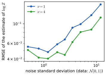
The finite-sample problem is a logistic regression. The classifier logit is \(\log\nu+\log p_{\bm\theta}-\log p_n=\log\nu-\bm\theta^\T\bm\phi(\bm x)+c-\log p_n(\bm x)\) with \(c=-\log Z\): linear in \((\bm\theta,c)\) for an exponential-family energy, so the NCE objective is convex and damped Newton finds the global optimum (the code does; a BFGS minimisation from a nearby point agrees to \(10^{-8}\), and the learned \(-c\) is within 0.005 of \(\log Z_{\bm\theta}\) of the fitted energy). In a Monte Carlo study (500 data points, 120 repetitions, \(N(0,1)\) data, Gaussian EBM) the root-mean-square error of the estimate of \(\log Z\) is smallest, 0.05, for noise standard deviation about 1 and grows to 0.17 for standard deviation 12 (\(\nu=1\); with four times more noise samples, 0.12): the benefit of extra noise samples is bounded, and noise much wider than the data wastes them (Figure 24.x7).
24.4.1 Connection to score matching
p. 862 Choosing the noise as a shifted copy of the data and a slightly different parametrisation of the classifier turns NCE into score matching (Gutmann and Hyvärinen 2012). For a small deterministic vector \(\bm v\) let \(p_n(\bm x)=p_{\mathcal D}(\bm x-\bm v)\): easy to sample (\(\bm x=\bm x'+\bm v\)) but with an unknown density. Replace \(p_n\) in (24.48) by the model's shifted density, \[ p_{n,\bm\theta}(y=0\given\bm x):=\frac{p_{\bm\theta}(\bm x-\bm v)}{p_{\bm\theta}(\bm x)+p_{\bm\theta}(\bm x-\bm v)} \tag{24.54} \] and the NCE objective (24.50) reduces to \[ \bm\theta^*=\arg\min_{\bm\theta}\E_{p_{\mathcal D}}\Big[\log\big(1+e^{E_{\bm\theta}(\bm x)-E_{\bm\theta}(\bm x-\bm v)}\big)+\log\big(1+e^{E_{\bm\theta}(\bm x)-E_{\bm\theta}(\bm x+\bm v)}\big)\Big]. \tag{24.55} \] At the optimum the posteriors match, \(\frac{p_{\bm\theta^*}(\bm x-\bm v)}{p_{\bm\theta^*}(\bm x)+p_{\bm\theta^*}(\bm x-\bm v)}=\frac{p_{\mathcal D}(\bm x-\bm v)}{p_{\mathcal D}(\bm x)+p_{\mathcal D}(\bm x-\bm v)}\) (24.56, 24.57), which the book takes to give \(p_{\bm\theta^*}=p_{\mathcal D}\). For \(\|\bm v\|\to0\) a Taylor expansion shows (24.55) is equivalent to the sliced score-matching objective (24.38) after averaging over a distribution of \(\bm v\), up to the terms hidden in \(o(\|\bm v\|^2)\) (24.58).
Filling the gap 24.12: the expansion of (24.55) with its correct constants, and why one direction \(\bm v\) does not identify the density pp. 862, (24.54)–(24.58)
Proof
The expansion. Let \(\bm g=\nabla E(\bm x)\), \(\bm H=\nabla^2E(\bm x)\), \(a_1=E(\bm x)-E(\bm x-\bm v)=\bm g^\T\bm v-\frac12\bm v^\T\bm H\bm v+O(\|\bm v\|^3)\) and \(a_2=E(\bm x)-E(\bm x+\bm v)=-\bm g^\T\bm v-\frac12\bm v^\T\bm H\bm v+O(\|\bm v\|^3)\), the cubic terms being equal and opposite in \(a_1,a_2\) so that they cancel in \(a_1+a_2\) and \(a_1^2+a_2^2\) to this order. Since \(\log(1+e^a)=\log2+\frac a2+\frac{a^2}8+O(a^4)\) (the cubic term vanishes because \(\log(1+e^a)-\frac a2\) is even), \[ \log(1+e^{a_1})+\log(1+e^{a_2})=2\log2+\frac{a_1+a_2}{2}+\frac{a_1^2+a_2^2}{8}+O(\|\bm v\|^4)=2\log2+\tfrac14(\bm v^\T\bm g)^2-\tfrac12\bm v^\T\bm H\bm v+O(\|\bm v\|^4). \] Therefore \[ \mathrm{(24.55)}=2\log2+\frac12\,\E_{p_{\mathcal D}}\Big[\tfrac12(\bm v^\T\nabla E)^2-\bm v^\T\nabla^2E\,\bm v\Big]+O(\|\bm v\|^4), \] that is, \(2\log2\) plus one half of the sliced score-matching integrand of gap 24.9 (with its correct minus sign), for the fixed direction \(\bm v\); averaging over a distribution of \(\bm v\) gives \(\frac12\mathrm D_{\mathrm{SF}}\) up to a constant. The printed (24.58) has prefactor \(\frac14\) on \(\frac12(\bm v^\T\nabla E)^2+\bm v^\T\bm H\bm v\), which has the wrong Hessian sign and half the weight on the first term. For a smooth 2-D energy and \(\|\bm v\|=0.1\) the relative error of the expansion above is 0.05%, and of the printed one 174%.
One direction is not enough. The matching of posteriors (24.56)–(24.57) says \(r(\bm x):=p_{\bm\theta^*}(\bm x)/p_{\mathcal D}(\bm x)\) satisfies \(r(\bm x-\bm v)=r(\bm x)\) for all \(\bm x\): \(r\) is periodic along \(\bm v\), which does not make it constant. Counterexample (1-D, \(v=1.3\)): \(p_{\mathcal D}=\N(0,1)\) and \(p_{\bm\theta}=p_{\mathcal D}\cdot(1+\frac12\sin(2\pi x/v))\); this integrates to one (the sine integrates to zero against the even density), has the same posteriors as \(p_{\mathcal D}\) at every \(x\) (to \(10^{-12}\)) and differs from it by up to 0.07 in density. The shifted-noise objective therefore identifies \(p_{\mathcal D}\) only if \(\bm v\) ranges over a set of directions and lengths that leaves no non-constant function periodic in all of them (for a continuous \(r\), all small \(\bm v\) in an open set suffice), which is exactly the setting of the sliced objective with \(p(\bm v)\) having a positive definite second moment.
24.5 Other methods
p. 862 Beyond MCMC maximum likelihood, score matching and NCE there are other ways to learn EBMs; the book surveys three.
24.5.1 Minimizing differences/derivatives of KL divergences
p. 863 The partition function often cancels in the difference of two related KL divergences, or in a derivative. In minimum velocity learning and minimum probability flow a Markov chain is designed with \(p_0=p_{\mathcal D}\) and \(p_\infty=p_{\bm\theta}\), and one minimises the speed of the evolution at \(t=0\), \[ \Big|\frac{\d}{\d t}\Dkl(p_t\|p_{\bm\theta})\Big|_{t=0}\quad\text{or}\quad\Big|\frac{\d}{\d t}\Dkl(p_{\mathcal D}\|p_t)\Big|_{t=0} \tag{24.59} \] which does not need \(Z_{\bm\theta}\). In minimum KL contraction a map \(\Phi\) with \(\Dkl(p\|q)\ge\Dkl(\Phi\{p\}\|\Phi\{q\})\), with equality iff \(p=q\), defines \[ \Dkl(p_{\mathcal D}\|p_{\bm\theta})-\Dkl(\Phi\{p_{\mathcal D}\}\|\Phi\{p_{\bm\theta}\}) \tag{24.60, 24.61} \] which is partition-function free when \(\Phi\) is linear. All three generalise score matching and NCE.
Filling the gap 24.13: the partition function cancels, the difference is a (generalised) CD objective, and a rate matrix built from energy differences p. 863, (24.59)–(24.61)
Proof
Cancellation and positivity. Let \(\Phi\) be a linear map that sends probability distributions to probability distributions (on a finite space, a column-stochastic matrix; in general a Markov kernel acting on laws), and \(u_{\bm\theta}=e^{-E_{\bm\theta}}\), \(p_{\bm\theta}=u_{\bm\theta}/Z\). Because \(\Phi\) is linear and conserves mass, \(\Phi\{p_{\bm\theta}\}=\Phi\{u_{\bm\theta}\}/Z\), so \[ \Dkl(p_{\mathcal D}\|p_{\bm\theta})=\E_{p_{\mathcal D}}\log p_{\mathcal D}+\E_{p_{\mathcal D}}E_{\bm\theta}+\log Z,\quad\Dkl(\Phi p_{\mathcal D}\|\Phi p_{\bm\theta})=\E_{\Phi p_{\mathcal D}}\log\Phi p_{\mathcal D}-\E_{\Phi p_{\mathcal D}}\log\Phi u_{\bm\theta}+\log Z, \] and the two \(\log Z\) terms cancel in (24.61): the objective is computable from \(E_{\bm\theta}\) alone. It is \(\ge0\) by the data-processing inequality (the Markov kernel contracts KL, as in gap 24.5), with equality iff \(p_{\mathcal D}=p_{\bm\theta}\) when \(\Phi\) strictly contracts. (Checked for a random energy and kernel on six states: the \(Z\)-free expression equals the definition to \(10^{-12}\), value 0.4977.) If \(\Phi\) is allowed to depend on \(\bm\theta\) through \(\Phi_{\bm\theta}p_{\bm\theta}=p_{\bm\theta}\) (a kernel with invariant law \(p_{\bm\theta}\)), the same formula is exactly \(\mathrm{CD}_T\) of (24.19) with \(\Phi=K_{\bm\theta}^T\): contrastive divergence is a minimum-KL-contraction objective whose map is the sampler.
A rate matrix without \(Z\). For a continuous-time chain with rates \(Q_{xy}=e^{(E(x)-E(y))/2}\) (\(x\ne y\)), \(p_{\bm\theta}(x)Q_{xy}=e^{-(E(x)+E(y))/2}/Z\) is symmetric in \((x,y)\): detailed balance, so \(p_{\bm\theta}\) is invariant, and \(Q\) uses only energy differences. If \(p_{\mathcal D}Q=0\) the data law is invariant, and for an ergodic chain it then equals \(p_{\bm\theta}\); the flow \(\|p_{\mathcal D}Q\|\) out of the data is the kind of quantity minimum probability flow drives to zero, again without \(Z\).
24.5.2 Minimizing the Stein discrepancy
pp. 863–864 The Stein discrepancy is \[ D_{\mathrm{Stein}}(p_{\mathcal D}\|p_{\bm\theta}):=\sup_{\bm f\in\mathcal F}\E_{p_{\mathcal D}}\big[\nabla_{\bm x}\log p_{\bm\theta}(\bm x)^\T\bm f(\bm x)+\tr(\nabla_{\bm x}\bm f(\bm x))\big] \tag{24.62} \] for a class \(\mathcal F\) of vector-valued functions; under regularity conditions it is \(\ge0\) with equality iff \(p_{\mathcal D}=p_{\bm\theta}\). Like score matching it needs only the model score. The trace term can be expensive; two ways around it are to take \(\mathcal F\) the unit ball of a reproducing kernel Hilbert space (the kernelised Stein discrepancy; Chwialkowski et al. 2016, Liu et al. 2016), or to estimate the trace by the Skilling–Hutchinson estimator.
Filling the gap 24.14: the Stein identity, why (24.62) is a discrepancy, and the closed form of the kernelised version pp. 863–864, (24.62)
Proof
The Stein identity. For a differentiable density \(p\) and a differentiable \(\bm f\) with \(p\bm f\to0\) at infinity, the divergence theorem gives \(\int\nabla\!\cdot(p\bm f)\,\d\bm x=0\), i.e. \[ \E_p\big[\nabla\log p^\T\bm f+\nabla\!\cdot\bm f\big]=0. \] So the Stein operator \(\mathcal A_p\bm f=\nabla\log p^\T\bm f+\nabla\!\cdot\bm f\) has mean zero under \(p\) (a 1-D numerical test with \(p=\N(0,1)\) and \(f=\cos x\,e^{-x^2/8}\): \(-5\times10^{-17}\); with the score of \(\N(1,1)\) instead: 0.60).
Why it is a discrepancy. Apply the identity to \(p_{\mathcal D}\) and subtract: for any \(\bm f\), \[ \E_{p_{\mathcal D}}[\mathcal A_{p_{\bm\theta}}\bm f]=\E_{p_{\mathcal D}}[\mathcal A_{p_{\bm\theta}}\bm f-\mathcal A_{p_{\mathcal D}}\bm f]=\E_{p_{\mathcal D}}\big[(\nabla\log p_{\bm\theta}-\nabla\log p_{\mathcal D})^\T\bm f\big]. \] It is \(0\) when the scores agree, so (24.62) vanishes if \(p_{\mathcal D}=p_{\bm\theta}\); since \(\bm f=\bm0\in\mathcal F\) (or \(\mathcal F\) is symmetric), the supremum is \(\ge0\). If \(\mathcal F\) is rich enough to contain a multiple of \(\nabla\log p_{\bm\theta}-\nabla\log p_{\mathcal D}\) (or is dense enough to approximate it), the supremum is strictly positive unless the scores agree, and (connected support) the densities then agree (gap 24.7). Only \(\nabla\log p_{\bm\theta}\) enters the left side, so the discrepancy can be computed without \(Z_{\bm\theta}\) and without \(\nabla\log p_{\mathcal D}\).
Closed form for the RKHS ball. Let \(\mathcal F=\{\bm f:\sum_i\|f_i\|_{\mathcal H}^2\le1\}\) with a continuously differentiable kernel \(k\), so that \(f_i(\bm x)=\langle f_i,k(\bm x,\cdot)\rangle\) and \(\partial_if_i(\bm x)=\langle f_i,\partial_ik(\bm x,\cdot)\rangle\). The functional \(\bm f\mapsto\E_{p_{\mathcal D}}[\mathcal A\bm f]\) is linear and bounded, equal to \(\sum_i\langle f_i,\xi_i\rangle\) with \(\xi_i=\E_{\bm x\sim p_{\mathcal D}}[s_i(\bm x)k(\bm x,\cdot)+\partial_ik(\bm x,\cdot)]\), \(\bm s=\nabla\log p_{\bm\theta}\). By Cauchy–Schwarz the supremum is \(\|\bm\xi\|\), and \[ \|\bm\xi\|^2=\E_{\bm x,\bm x'\sim p_{\mathcal D}}\Big[\bm s(\bm x)^\T\bm s(\bm x')k(\bm x,\bm x')+\bm s(\bm x)^\T\nabla_{\bm x'}k+\bm s(\bm x')^\T\nabla_{\bm x}k+\tr(\nabla_{\bm x}\nabla_{\bm x'}k)\Big] \] by the reproducing property again. This kernelised Stein discrepancy involves no Jacobian of a function \(\bm f\): the derivatives fall on the kernel, which is the sense in which "the trace term is a constant" in the book's account (it does not need to be optimised over \(\bm f\)). It is estimated by a U-statistic over pairs of sample points. For \(p_{\bm\theta}=\N(0,1)\) and 1 500 samples with a Gaussian kernel of width 1, the estimate of the squared discrepancy is 0.0014 when the samples come from the model and 0.11, 0.50, 1.18 when they are shifted by 0.5, 1, 1.5: zero for the model, increasing in the mismatch.
24.5.3 Adversarial training
pp. 864–865 Maximum likelihood needs model samples at every step; one can instead learn a fast auxiliary sampler \(q_{\bm\phi}\) adversarially. Introduce \(q_{\bm\phi}\) in the log-partition function and apply Jensen's inequality: \[ \E_{p_{\mathcal D}}[\log p_{\bm\theta}]=\E_{p_{\mathcal D}}[-E_{\bm\theta}]-\log\int q_{\bm\phi}\frac{e^{-E_{\bm\theta}}}{q_{\bm\phi}}\d\bm x\le\E_{p_{\mathcal D}}[-E_{\bm\theta}]-\E_{q_{\bm\phi}}[-E_{\bm\theta}]-\Hent(q_{\bm\phi}) \tag{24.63} \] an upper bound on the expected log-likelihood. Minimising it over \(\bm\phi\) tightens it, maximising it over \(\bm\theta\) is a surrogate for maximum likelihood, giving the minimax problem \[ \max_{\bm\theta}\min_{\bm\phi}\ \E_{q_{\bm\phi}}[E_{\bm\theta}]-\E_{p_{\mathcal D}}[E_{\bm\theta}]-\Hent(q_{\bm\phi}) \tag{24.64} \] similar to a GAN (Chapter 26). It needs a sampler \(q_{\bm\phi}\) that is both fast to sample and has a tractable entropy, which restricts it to invertible models such as inverse autoregressive flows (Dai et al. 2019b). Neural samplers \(\bm x=g_{\bm\phi}(\bm z)\) have an intractable entropy, approximated by heuristics, by the identity \(\Hent(q_{\bm\phi})=\MI(g_{\bm\phi}(\bm z),\bm z)\) with a variational lower bound on mutual information (Kumar et al. 2019), or, for a base density \(p_0\) with \(p_{\bm\theta}=p_0e^{-E_{\bm\theta}}/Z\), by replacing \(-\Hent(q_{\bm\phi})\) with \(\Dkl(q_{\bm\phi}\|p_0)\) (Dai et al. 2019a). A noisy neural sampler \(g_{\bm\phi}(\bm z)+\sigma\bm\epsilon\) has an easily estimated entropy gradient (Grathwohl et al. 2020); Xie et al. (2018) train the sampler with MCMC samples and use it to initialise chains (cooperative sampling, not optimising (24.63)); Yu et al. (2020) allow any \(f\)-divergence.
Filling the gap 24.15: the exact slack of the adversarial bound, and when the inner minimisation is tight p. 864, (24.63)–(24.64)
Proof
The slack. For any density \(q\) with \(\Dkl(q\|p_{\bm\theta})<\infty\), \[ \Dkl(q\|p_{\bm\theta})=\E_q\log q+\E_q[E_{\bm\theta}]+\log Z_{\bm\theta}\ \Longrightarrow\ \log Z_{\bm\theta}=\E_q[-E_{\bm\theta}]+\Hent(q)+\Dkl(q\|p_{\bm\theta}). \] Since \(\Dkl\ge0\), \(\log Z_{\bm\theta}\ge\E_q[-E_{\bm\theta}]+\Hent(q)\) (the Jensen step (i) of the book), and the expected log-likelihood is \(\E_{p_{\mathcal D}}[-E_{\bm\theta}]-\log Z_{\bm\theta}=\text{bound (24.63)}-\Dkl(q\|p_{\bm\theta})\). So (24.63) is an upper bound on \(\ell\) with slack exactly \(\Dkl(q_{\bm\phi}\|p_{\bm\theta})\), tight iff \(q_{\bm\phi}=p_{\bm\theta}\): minimising over \(\bm\phi\) is minimising the KL from the sampler to the model, and (24.64) at the inner optimum recovers \(\ell\) itself when the sampler family contains \(p_{\bm\theta}\). With \(E=\bm\theta^\T\bm\phi\) from the quartic family and a Gaussian \(q\) the identity holds to \(10^{-4}\) in a quadrature test (0.8311 on both sides), the slack being positive.
The game. The outer problem maximises over \(\bm\theta\) the minimum over \(\bm\phi\) of the bound, and \(\min_{\bm\phi}\) of the bound is an upper bound on \(\ell(\bm\theta)\) that is tight only if the sampler family contains \(p_{\bm\theta}\): with a restricted family the outer maximisation ascends an upper bound, not \(\ell\), and the quality of the surrogate is governed by the sampler's expressiveness. For \(p_{\bm\theta}=p_0e^{-E_{\bm\theta}}/Z_{\bm\theta}\) with a fixed base density \(p_0\) the same algebra gives \(\log Z_{\bm\theta}=\E_q[-E_{\bm\theta}]-\Dkl(q\|p_0)+\Dkl(q\|p_{\bm\theta})\), which is why the entropy term can be traded for a KL divergence to the base density (Dai et al. 2019a).
Practice problems
The book has no end-of-chapter exercises for Chapter 24, so here are three short problems of my own, with complete solutions (hidden).
Practice problem 24.1 (how much noise can denoising score matching take?). Data \(x\sim\N(0,1)\), energy \(E_a(x)=\frac a2x^2\). (a) Find the DSM optimum \(a^*(\sigma)\). (b) How large may \(\sigma\) be if the fitted variance \(1/a^*\) must exceed the true one by at most 5%? (c) For that \(\sigma\), what is the standard deviation of one per-sample DSM gradient at \(a=1/1.05\)?
Solution
(a) The noisy data are \(\tilde x\sim\N(0,1+\sigma^2)\) and DSM fits the score of \(q\), \(-\tilde x/(1+\sigma^2)\) (gap 24.8), so \(a^*=1/(1+\sigma^2)\). Directly: the loss \(\frac12\E(-a\tilde x+z/\sigma)^2\) has derivative \(a\E\tilde x^2-\E[z\tilde x]/\sigma=a(1+\sigma^2)-1\), zero at \(a^*\). (b) \(1/a^*=1+\sigma^2\le1.05\) gives \(\sigma\le\sqrt{0.05}=0.2236\). (c) The per-sample gradient is \(a\tilde x^2-z\tilde x/\sigma\) with \(\tilde x=x+\sigma z\); simulating \(2\times10^5\) draws at \(\sigma=0.2236\), \(a=1/1.05\) gives a standard deviation of 4.51, about \(1/\sigma=4.47\) as predicted. So a 5% variance bias already costs a gradient noise of about 4.5 times the signal scale; antithetic noise pairs reduce it to about 2.
Practice problem 24.2 (a step size for the unadjusted Langevin chain). Target \(\N(0,1/a)\). (a) What is the largest \(\epsilon\) for which the stationary variance of (24.18) is within 5% of \(1/a\)? (b) What is the largest stable \(\epsilon\)? (c) For the wells of expert A (\(a\approx4.94\)) give both numbers.
Solution
By gap 24.3 the stationary variance is \(\frac1a\cdot\frac1{1-\epsilon^2a/4}\). (a) \(\frac1{1-\epsilon^2a/4}\le1.05\iff\epsilon^2a/4\le1-\frac1{1.05}=0.04762\iff\epsilon\le\frac{0.4364}{\sqrt a}\) (simulating the variance recursion at \(\epsilon=0.4364/\sqrt a\) gives 1.0500). (b) Stability needs \(|1-\epsilon^2a/2|<1\iff\epsilon<2/\sqrt a\). (c) With \(a=4.94\): \(\epsilon\le0.196\) for 5% accuracy and \(\epsilon<0.900\) for stability. Hence a step of 0.3 (the demonstration's default for the product of experts) is stable but biased by about 12% in the well variance, and 1.0 diverges; a Metropolis correction removes the bias and the instability at the price of rejecting a share of the moves.
Practice problem 24.3 (the weight of NCE). Data and model are \(\N(0,1)\) and \(\nu=1\). Compute the weight \(w(x)=p_n(x)/(p_n(x)+p_{\bm\theta}(x))\) in the NCE gradient (gap 24.11) at \(x=2\) for noise \(\N(0,0.3^2)\), \(\N(0,1)\) and \(\N(0,3^2)\), and say what it means for learning.
Solution
\(p_{\bm\theta}(2)=\frac{e^{-2}}{\sqrt{2\pi}}=0.0540\). Noise \(\N(0,s^2)\): \(p_n(2)=\frac{e^{-2/s^2}}{s\sqrt{2\pi}}\). For \(s=0.3\): \(e^{-22.2}/0.752=2.9\times10^{-10}\), weight \(5.5\times10^{-9}\). For \(s=1\): \(p_n=p_{\bm\theta}\), weight \(\frac12\). For \(s=3\): \(e^{-0.222}/7.52=0.1065\), weight \(0.1065/(0.1065+0.0540)=0.66\). The NCE gradient at points like \(x=2\) is effectively switched off for the narrow noise: the classifier separates noise from data using the region \(|x|<1\) only and the tails of the data are never used, so the learned shape and \(Z\) are poor (the failing preset of the demonstration); for wide noise the data region is fully weighted.
Demonstrations
- Fitting an energy without its partition function (Sections 24.2, 24.3, 24.4): the quartic energy fitted by maximum likelihood, score matching, denoising score matching and NCE; the noise level \(\sigma\), the noise width and the KL to the truth.
- A product of experts, sampled by Langevin dynamics (Sections 24.1.1, 24.2.1): four wells, a half-plane constraint, their sum; unadjusted and Metropolis-adjusted chains, the step size, instability and the exact stationary variance.
- Contrastive divergence on a tiny RBM (Section 24.2.2): exact maximum likelihood against CD-\(k\) and persistent CD, with every expectation computed exactly.
Python code for every figure: code index. Data used by the demos: data/ch24-estimators.json, data/ch24-poe.json, data/ch24-rbm.json. Companion demos: HMC and MALA and the Ising and Potts models.
Notes on the book
Points where the book is imprecise or wrong
- Section 24.1. "The energy function can be any kind of function that returns a non-negative scalar": the only requirement is \(Z_{\bm\theta}=\int e^{-E_{\bm\theta}}<\infty\); energies may be negative (adding a constant to \(E\) only rescales \(Z\)), and for a product of experts one of the experts may even be non-normalisable (gap 24.1).
- (24.20) versus (24.21). With \(p\propto e^{-E}\) the gradient is "clamped minus unclamped" for the log-linear energy \(E=-\bm x^\T\bm W\bm z-\bm b^\T\bm x-\bm c^\T\bm z\); the printed plus signs reverse it (gap 24.4).
- Algorithm 24.2, line 10. \(\bm g_t=-\frac1B\sum_b\bm g_b-\frac1S\sum_s\tilde{\bm g}_s\) has the same sign on the data and model terms, so the update has no fixed point; the second term must be added (gap 24.6). The text also refers to the pseudocode as "Algorithm 12".
- (24.38) and (24.41). The Hessian term \(\sum_{i,j}\partial_i\partial_jE\,v_iv_j\) must carry a minus sign when \(\sc=-\nabla E\); (24.42), written with the Jacobian of the score, has the correct sign (gap 24.9).
- (24.36). "\(+\)constant" hides terms of order one that depend on \(\bm\theta\); only the two divergent terms are dropped, and only the cross term \(\bm z^\T\sc/\sigma\) affects the gradient (gap 24.8).
- (24.44)–(24.45). The second expectation in (24.44) must be over the data (the chain starts at the data), and the one-step Langevin CD gradient of the log-likelihood is \(-\frac{\epsilon^2}{2}\nabla_{\bm\theta}\DF(p_{\mathcal D}\|p_{\bm\theta})+o(\epsilon^2)\), with a minus sign (gap 24.10). (24.43) and (24.18) use different step-size conventions (\(\epsilon\) and \(\epsilon^2\)).
- De Bruijn's identity (Section 24.3.4). With \(\DF\) defined by (24.28), including the factor \(\frac12\), the identity is \(\frac{\d}{\d t}\Dkl(q_t\|p_{\bm\theta,t})=-\DF(q_t\|p_{\bm\theta,t})\), not \(-\frac12\DF\) (gap 24.10).
- (24.57)–(24.58). Matching the posteriors for a single shift \(\bm v\) only makes \(p_{\bm\theta}/p_{\mathcal D}\) periodic along \(\bm v\), not constant; and the small-\(\bm v\) expansion is \(2\log2+\frac12\E[\frac12(\bm v^\T\nabla E)^2-\bm v^\T\nabla^2E\,\bm v]+O(\|\bm v\|^4)\), not the printed \(\frac14\E[\frac12(\cdot)^2+\bm v^\T\bm H\bm v]\) (gap 24.12).
- Section 24.5.2. "The trace term is a constant and does not affect optimization" for the kernelised discrepancy: the Jacobian of \(\bm f\) is not constant, it is evaluated through derivatives of the kernel (gap 24.14).
- Figure references. The text of Sections 24.2.1 and 24.3.1 refers to "Figure 25.5" (Chapter 25) for the Langevin and score-matching examples; the pseudocode reference "Algorithm 12" in 24.2.2.2 should be Algorithm 24.2.
References
- Murphy, K. P. (2023). Probabilistic Machine Learning: Advanced Topics. MIT Press, Cambridge, MA. Chapter 24 (with Y. Song and D. P. Kingma), pp. 849–865, and supplementary material, Chapter 24. probml.github.io/pml-book/book2.html.
- Chwialkowski, K., Strathmann, H. and Gretton, A. (2016). A kernel test of goodness of fit. International Conference on Machine Learning. Liu, Q., Lee, J. D. and Jordan, M. (2016). A kernelized Stein discrepancy for goodness-of-fit tests. International Conference on Machine Learning.
- Dai, B., Liu, Z., Dai, H., He, N., Gretton, A., Song, L. and Schuurmans, D. (2019). Exponential family estimation via adversarial dynamics embedding. Advances in Neural Information Processing Systems, 32. Dai, Z., Almahairi, A., Bachman, P., Hovy, E. and Courville, A. (2019). Calibrating energy-based generative adversarial networks. International Conference on Learning Representations.
- Du, Y. and Mordatch, I. (2019). Implicit generation and modeling with energy-based models. Advances in Neural Information Processing Systems, 32. Du, Y., Li, S., Tenenbaum, J. and Mordatch, I. (2020). Improved contrastive divergence training of energy based models.
- Grathwohl, W., Wang, K.-C., Jacobsen, J.-H., Duvenaud, D. and Zemel, R. (2020). Learning the Stein discrepancy for training and evaluating energy-based models without sampling. International Conference on Machine Learning.
- Gutmann, M. and Hyvärinen, A. (2010). Noise-contrastive estimation: a new estimation principle for unnormalized statistical models. AISTATS. Gutmann, M. U. and Hirayama, J. (2012). Bregman divergence as general framework to estimate unnormalized statistical models. Uncertainty in Artificial Intelligence. Gutmann, M. U. and Hyvärinen, A. (2012). Noise-contrastive estimation of unnormalized statistical models, with applications to natural image statistics. Journal of Machine Learning Research, 13, 307–361.
- Hinton, G. E. (2002). Training products of experts by minimizing contrastive divergence. Neural Computation, 14(8), 1771–1800.
- Hyvärinen, A. (2005). Estimation of non-normalized statistical models by score matching. Journal of Machine Learning Research, 6, 695–709. Hyvärinen, A. (2007). Connections between score matching, contrastive divergence, and pseudolikelihood for continuous-valued variables. IEEE Transactions on Neural Networks, 18(5), 1529–1531.
- Kim, T. and Bengio, Y. (2016). Deep directed generative models with energy-based probability estimation. arXiv:1606.03439. Kumar, R., Ozair, S., Goyal, A., Courville, A. and Bengio, Y. (2019). Maximum entropy generators for energy-based models. arXiv:1901.08508.
- Lyu, S. (2011). Unifying non-maximum likelihood learning objectives with minimum KL contraction. Advances in Neural Information Processing Systems, 24. Sohl-Dickstein, J., Battaglino, P. and DeWeese, M. (2011). Minimum probability flow learning. International Conference on Machine Learning. Movellan, J. R. (2008). Contrastive divergence in Gaussian diffusions. Neural Computation, 20(9), 2238–2252.
- Mnih, A. and Teh, Y. W. (2012). A fast and simple algorithm for training neural probabilistic language models. International Conference on Machine Learning.
- Skilling, J. (1989). The eigenvalues of mega-dimensional matrices. In Maximum Entropy and Bayesian Methods. Hutchinson, M. F. (1989). A stochastic estimator of the trace of the influence matrix for Laplacian smoothing splines. Communications in Statistics: Simulation and Computation, 18(3), 1059–1076.
- Song, Y., Garg, S., Shi, J. and Ermon, S. (2019). Sliced score matching: a scalable approach to density and score estimation. Uncertainty in Artificial Intelligence.
- Tieleman, T. (2008). Training restricted Boltzmann machines using approximations to the likelihood gradient. International Conference on Machine Learning. Younes, L. (1999). On the convergence of Markovian stochastic algorithms with rapidly decreasing ergodicity rates. Stochastics and Stochastics Reports, 65, 177–228.
- Vincent, P. (2011). A connection between score matching and denoising autoencoders. Neural Computation, 23(7), 1661–1674.
- Xie, J., Lu, Y., Zhu, S.-C. and Wu, Y. N. (2016). A theory of generative ConvNet. International Conference on Machine Learning. Xie, J., Lu, Y., Gao, R. and Wu, Y. N. (2018). Cooperative learning of energy-based model and latent variable model via MCMC teaching. AAAI.
- Yu, L., Song, Y., Song, J. and Ermon, S. (2020). Training deep energy-based models with f-divergence minimization. International Conference on Machine Learning.
The numerical statements in the text (the gradient and Hessian of the log partition function, the moment-matching conditions and the unbiasedness of the Monte Carlo estimate; the stationary variance and stability limit of discretised Langevin dynamics and the correctness of the Metropolis-adjusted chain; the Gaussian product of experts and the half-plane mass of the example; the RBM conditionals, gradient, reversibility of the Gibbs sweep and the exact CD, PCD and maximum-likelihood learning curves; the closed-form score-matching and denoising solutions, Vincent's identity, Tweedie's formula, the bias and variance of DSM; the sliced objective with its sign, the Hessian-vector trick and the trace-estimator variances; the one-step Langevin expansion and de Bruijn's identity; the NCE gradient, optimum and expansion; KL contraction, the Stein identity and the kernelised Stein discrepancy; and the adversarial slack) were confirmed numerically.