Variational inference
Variational inference (VI) turns the computation of a posterior into an optimisation problem: choose a tractable family of distributions and find the member closest, in KL divergence, to the posterior. The quantity optimised, the evidence lower bound (ELBO), is also a lower bound on the log marginal likelihood, so the same machinery fits model parameters (variational EM), selects models and trains deep latent-variable models. The chapter covers the two ways of doing the optimisation: gradient-based VI for a chosen parametric family (reparameterisation, automatic-differentiation VI, score-function gradients with control variates) and coordinate ascent for factorised families (mean field for Ising models, Gaussians and mixtures, variational message passing). It then improves the family (structured, hierarchical, flow and implicit posteriors), the bound (importance weighting, thermodynamic integration, the evidence upper bound, wake-sleep) and the divergence (expectation propagation). The supplement adds more Gaussian VI, online VI, conjugate-computation VI and the variational view of belief propagation. The notes prove the steps the book leaves out and test the claims numerically and on data.
Ch. 1 Introduction Ch. 2 Probability Ch. 3 Statistics Ch. 4 Graphical models Ch. 5 Information theory Ch. 6 Optimisation Ch. 7 Inference algorithms Ch. 8 Gaussian filtering Ch. 9 Message passing Ch. 10 Variational inference Ch. 11 Monte Carlo Ch. 12 MCMC Ch. 13 Sequential Monte Carlo Ch. 14 Predictive models Ch. 15 GLMs Ch. 16 Deep networks Ch. 17 Bayesian neural networks Ch. 18 Gaussian processes Ch. 19 Beyond iid Ch. 20 Generative models Ch. 21 VAEs Ch. 22 Autoregressive models Ch. 23 Normalizing flows Ch. 24 Energy-based models Ch. 25 Diffusion models Ch. 26 GANs Ch. 27 Discovery methods Ch. 28 Latent factor models Ch. 29 State-space models Ch. 30 Graph learning Ch. 31 Nonparametric Bayes Ch. 32 Representation learning Ch. 33 Interpretability Ch. 34 Decision making Ch. 35 Reinforcement learning Ch. 36 Causality
How to read these notes
They follow the book. Sections carry the book's numbers and equations the book numbers keep their numbers, e.g. \((10.9)\); equations without a number are steps the book skips. Sections from the online supplement are labelled supplement and placed where the book refers to them (supplement equations are written S(10.n)).
Filling the gaps. Wherever the book writes "one can show", leaves a step to the reader, or quotes a result from the literature, an orange Filling the gap box gives the full argument. Proofs start hidden: open one with its bar, or use the buttons below. Results already proved in full elsewhere on the site (the score-function and reparameterisation estimators, Bonnet's and Price's theorems, the EM monotonicity, the VB updates for the univariate Gaussian and for the Gaussian mixture) are stated and linked rather than repeated.
Figures and demonstrations. Every computed figure is reproduced by the Python code; Figures 10.1, 10.3, 10.4, 10.5, 10.8, S10.5 and S10.6 are diagrams and are not reproduced. Data: Old Faithful for Figures 10.7 and 10.12 to 10.14; a synthetic letter image for Figure 10.9; simulated data elsewhere. The supplement's Africa ruggedness data are not available here, so Figures S10.1 to S10.3 use a stand-in with the same structure (scikit-learn's diabetes data); the captions say so. Three extra figures (10.x1 to 10.x3) illustrate results proved here. The ▶ Demo boxes open an interactive demonstration set to the case being discussed.
Main reference
K. P. Murphy, Probabilistic Machine Learning: Advanced Topics, MIT Press (2023; online draft of December 2025), Chapter 10, pages 439–482 (book page: probml.github.io/pml-book/book2.html), and the supplementary material, Chapter 10. Section, equation, figure and algorithm numbers below refer to this book. The explanations, derivations, figures and code are my own. The book has no end-of-chapter exercises for this chapter; three practice problems are given instead.
Companion courses
The classical material of the chapter is developed in full in Chapter 10 of the Bishop course, and those proofs are not repeated: the optimal mean-field factor (gap 10.2 there), variational Bayes for the univariate Gaussian (gaps 10.3–10.5), the variational Gaussian mixture (gaps 10.6–10.9) and expectation propagation for the clutter problem (Section 10.7 there). Earlier chapters of this course supply the tools: the score-function and reparameterisation gradients with control variates (gap 6.3, gap 6.5), Bonnet's and Price's theorems (gap 6.4), natural gradients for exponential families (gap 6.11), EM and variational EM (gap 6.14), and the two KL projections (gap 5.4, gap 5.5). Related demonstrations: VB for a Gaussian, the variational mixture of Gaussians, EP for the clutter problem, diagonal Gaussian approximations, posterior approximations for a coin.
What this chapter adds: the ELBO identities with their conditions, why the gradient can be pushed inside the expectation for \(\bm\theta\) but not for \(\bm\phi\), the reparameterised densities for the three Gaussian families and the \(O(d)\) algebra of the low-rank one, ADVI's Jacobian term, the optimal control-variate constant, the mean-field Ising and digamma-shrinkage dynamics, the closed-form VB lower bound, variational message passing, the IWAE monotonicity proof, thermodynamic integration, the EUBO and wake-sleep gradients, the EP fixed-point characterisation, and from the supplement the sparsity of the optimal Gaussian precision, the FOO-VB/BGD updates, conjugate-computation VI, and the Bethe, mean-field and tree-reweighted bounds on \(\log Z\).
The chapter at a glance
- 10.1 The ELBO and the free energy (gap 10.1); variational EM and empirical Bayes (10.2); minibatches and amortisation (10.3).
- 10.2 Which gradients pass inside the expectation (gap 10.4); reparameterised densities (10.5), low rank (10.6); sparse Gaussian VI (10.7); ADVI (10.8); REINFORCE and control variates (10.9); FOO-VB and BGD (10.10).
- 10.3 CAVI and its convergence (gap 10.11); mean-field Ising (10.12); the VB Gaussian bound (10.13); VEM from VBEM (10.14); digamma shrinkage (10.15); \(\log K!\) (10.16); VMP (10.17); CVI (10.18).
- 10.4 Factorial HMMs (gap 10.19); auxiliary-variable bounds (10.20); implicit posteriors (10.21); graphical models: exact, mean field, Bethe, tree-reweighted (10.22–10.24).
- 10.5–10.6 IWAE (gap 10.25); TVO (10.26); EUBO (10.27); wake-sleep (10.28).
- 10.7 EP fixed points and moment matching (gap 10.29); ADF, damping and power EP (10.30).
Notation. \(p_{\bm\theta}(\bm x,\bm z)\) is the joint, \(q_{\bm\psi}(\bm z)\) the variational distribution with variational parameters \(\bm\psi\) (\(\bm\phi\) for an inference network). \(\ELBO\) is the ELBO (maximised), \(\VFE=-\ELBO\) the variational free energy (minimised). \(\Hent(q)=-\E_q\log q\) is the (differential) entropy. \(\Ga(\lambda\given a,b)\propto\lambda^{a-1}e^{-b\lambda}\) uses the rate \(b\). \(\sigm(a)=1/(1+e^{-a})\), \(\dg\) is the digamma function. Logarithms are natural.
Prerequisites. Chapters 2 to 6 of the book (exponential families, KL divergence, the two Monte Carlo gradient estimators, EM), and Chapter 10 of the Bishop course.
10.1 Introduction
p. 439 Variational inference reduces posterior inference to optimisation. The book's treatment is an overview with pointers to the literature; these notes add the arguments behind each step.
See also: Section 7.4.4 of these notes (VI in the inference overview); Bishop course, Section 10.1.
10.1.1 The variational objective
pp. 439–441 Latent variables \(\bm z\), data \(\bm x\), fixed parameters \(\bm\theta\): the posterior \(p_{\bm\theta}(\bm z\given\bm x)=p_{\bm\theta}(\bm x,\bm z)/p_{\bm\theta}(\bm x)\) has an intractable normaliser \(p_{\bm\theta}(\bm x)=\int p_{\bm\theta}(\bm x,\bm z)\d\bm z\). VI looks for \[ \bm\psi^*=\argmin_{\bm\psi}\Dkl\big(q_{\bm\psi}(\bm z)\,\|\,p_{\bm\theta}(\bm z\given\bm x)\big), \tag{10.2} \] which is a minimisation over functions (a variational problem) restricted to a parametric family. Expanding the posterior, the intractable \(\log p_{\bm\theta}(\bm x)\) separates as an additive constant, leaving the loss \[ \VFE(\bm\theta,\bm\psi\given\bm x)=\E_{q_{\bm\psi}(\bm z)}\big[-\log p_{\bm\theta}(\bm x,\bm z)+\log q_{\bm\psi}(\bm z)\big]. \tag{10.5} \]
10.1.1.1 The view from physics: minimise the variational free energy
p. 440 With energy \(\mathcal E_{\bm\theta}(\bm z)=-\log p_{\bm\theta}(\bm x,\bm z)\), \(\VFE=\E_q[\mathcal E_{\bm\theta}]-\Hent(q)\) (10.6), expected energy minus entropy, and \[ \Dkl(q_{\bm\psi}\|p_{\bm\theta}(\cdot\given\bm x))=\VFE(\bm\theta,\bm\psi\given\bm x)+\log p_{\bm\theta}(\bm x)\ge0, \tag{10.7} \] so the VFE is an upper bound on the free energy \(-\log p_{\bm\theta}(\bm x)\) (10.8).
10.1.1.2 The view from statistics: maximise the evidence lower bound
pp. 440–441 The ELBO is \(\ELBO=-\VFE\): \[ \ELBO(\bm\theta,\bm\psi\given\bm x)=\E_{q_{\bm\psi}}[\log p_{\bm\theta}(\bm x,\bm z)-\log q_{\bm\psi}(\bm z)]\le\log p_{\bm\theta}(\bm x). \tag{10.9, 10.10} \] Two rewritings: "expected log joint plus entropy" (10.11)–(10.12), and \[ \ELBO=\E_{q_{\bm\psi}}[\log p_{\bm\theta}(\bm x\given\bm z)]-\Dkl\big(q_{\bm\psi}(\bm z)\|p_{\bm\theta}(\bm z)\big), \tag{10.14} \] "expected log likelihood minus KL from posterior to prior": the KL term is a regulariser keeping \(q\) near the prior.
Filling the gap 10.1: the ELBO identities, when they hold, and what maximising the ELBO does pp. 439–441, (10.1)–(10.15)
Proof
Setting. Fix \(\bm x\) with \(0<p_{\bm\theta}(\bm x)<\infty\). Let \(q\) be a density with \(\E_q|\log p_{\bm\theta}(\bm x,\bm z)|<\infty\) and finite entropy, so every expectation below is finite. If \(q\) puts mass where \(p_{\bm\theta}(\bm x,\bm z)=0\), the ELBO is \(-\infty\) and all statements hold trivially.
Identity (10.7). On \(\{q>0\}\), \(\log q-\log p(\bm z\given\bm x)=\log q-\log p(\bm x,\bm z)+\log p(\bm x)\). Taking \(\E_q\) of both sides (each term integrable) gives \(\Dkl(q\|p(\cdot\given\bm x))=\VFE+\log p(\bm x)\), i.e. \[ \log p_{\bm\theta}(\bm x)=\ELBO(q)+\Dkl\big(q\,\|\,p_{\bm\theta}(\cdot\given\bm x)\big). \] Since KL \(\ge0\) with equality iff \(q=p(\cdot\given\bm x)\) almost everywhere (Volume 1, Result 6.2), (10.8) and (10.10) follow, with equality exactly at the posterior. Because \(\log p_{\bm\theta}(\bm x)\) does not depend on \(\bm\psi\), the maximisers of \(\ELBO\) over \(\bm\psi\) and the minimisers of the KL coincide, and the gap at the optimum is the residual KL.
(10.11) and (10.14). Splitting \(\log p(\bm x,\bm z)-\log q\) as written gives (10.11). Writing \(\log p(\bm x,\bm z)=\log p(\bm x\given\bm z)+\log p(\bm z)\) and grouping \(\E_q[\log p(\bm z)-\log q(\bm z)]=-\Dkl(q\|p(\bm z))\) gives (10.14). Numerically, for the 2d Gaussian example of Figure 10.2 and an arbitrary Gaussian \(q\), \(\ELBO+\Dkl\) equals the exact log evidence to \(10^{-9}\).
Interpretation of (10.12). The "joint MAP" reading of the first term is exact in the limit: over all \(q\), \(\E_q[\log p(\bm x,\bm z)]\le\sup_{\bm z}\log p(\bm x,\bm z)\), with equality only for \(q\) concentrated on the maximisers; the entropy term pays for spreading out. \(\square\)
10.1.2 Form of the variational posterior
pp. 441–442 Two strategies: fixed-form VI picks a parametric family (say a Gaussian) and optimises the ELBO by gradients (Section 10.2); free-form VI assumes only the mean-field factorisation \(q(\bm z)=\prod_jq_j(\bm z_j)\) (10.16) and lets the optimal factors emerge from coordinate ascent (Section 10.3). The example: \(\bm z\in\R^2\) is the mean of a Gaussian with known covariance \(\bm\Sigma\), prior \(\N(\bm z\given\breve{\bm m},\breve{\bm V})\), likelihood \(\prod_n\N(\bm x_n\given\bm z,\bm\Sigma)\propto\N(\bar{\bm x}\given\bm z,\bm\Sigma/N)\) (10.17), with the Gaussian posterior of Section 3.4.4.
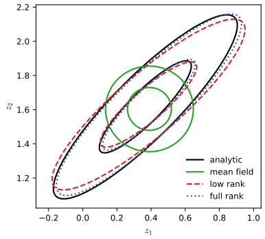
The mean-field fit underestimates the spread because minimising \(\Dkl(q\|p)\) is mode seeking (Section 5.1.4.3). The optimal diagonal Gaussian for a Gaussian target is derived in gap 5.5: same mean, variances \(1/\Lambda_{ii}\le\Sigma_{ii}\), with equality only for uncorrelated coordinates. Here \(1/\Lambda_{ii}=0.0156\) against the marginal variance \(0.0725\): the mean-field standard deviation (0.125) is less than half the true one (0.269).
See also: the diagonal Gaussian approximation demo (Chapter 5).
10.1.3 Parameter estimation using variational EM
pp. 442–444 To estimate \(\bm\theta\) by maximum likelihood when \(\log p(\mathcal D\given\bm\theta)=\sum_n\log p(\bm x_n\given\bm\theta)\) (10.18) is intractable, use the per-example bound \(\ELBO(\bm\theta,\bm\psi_n\given\bm x_n)\le\log p(\bm x_n\given\bm\theta)\) (10.21) and maximise their sum (10.22) alternately in \(\{\bm\psi_n\}\) (E step) and \(\bm\theta\) (M step): variational EM. For a fully observed model with hyper-parameters \(\bm\xi\) (10.23), the same bound \[ \log p(\mathcal D\given\bm\xi)\ge\E_{q_{\bm\psi}(\bm\theta)}\Big[\sum_n\log p(\bm x_n\given\bm\theta)\Big]-\Dkl\big(q_{\bm\psi}(\bm\theta)\|p(\bm\theta\given\bm\xi)\big) \tag{10.26} \] gives empirical Bayes (Section 3.7) when maximised over \((\bm\psi,\bm\xi)\), and variational Bayes when \(\bm\xi\) is fixed.
Filling the gap 10.2: variational EM never decreases the bound, and (10.26) is (10.14) for the parameter posterior pp. 443–444, (10.21)–(10.26)
Proof
(10.21)–(10.22). Apply gap 10.1 to each \(\bm x_n\) with its own \(q_{\bm\psi_n}(\bm z_n)\): \(\log p(\bm x_n\given\bm\theta)=\ELBO(\bm\theta,\bm\psi_n\given\bm x_n)+\Dkl(q_{\bm\psi_n}\|p(\bm z_n\given\bm x_n,\bm\theta))\). Summing over the independent examples gives (10.22), with gap \(\sum_n\Dkl(\cdot)\).
Monotonicity. Write \(F(\bm\theta,\bm\psi)=\sum_n\ELBO(\bm\theta,\bm\psi_n\given\bm x_n)\). An E step chooses \(\bm\psi^{t+1}\) with \(F(\bm\theta^t,\bm\psi^{t+1})\ge F(\bm\theta^t,\bm\psi^t)\); an M step chooses \(\bm\theta^{t+1}\) with \(F(\bm\theta^{t+1},\bm\psi^{t+1})\ge F(\bm\theta^t,\bm\psi^{t+1})\). Hence \(F\) never decreases and, being bounded above by \(\log p(\mathcal D\given\bm\theta)\le\sup_{\bm\theta}\log p(\mathcal D\given\bm\theta)\) when that is finite, converges. Unlike exact EM, the log likelihood itself need not increase: it is only sandwiched, \(F\le\log p(\mathcal D\given\bm\theta^t)\). If the family contains the exact posterior, the E step closes the gap and the method is exact EM, whose likelihood monotonicity and stationary points are proved in gap 6.14.
(10.26). The latent variable is now \(\bm\theta\) with prior \(p(\bm\theta\given\bm\xi)\) and likelihood \(\prod_np(\bm x_n\given\bm\theta)\); (10.14) with \(\bm z\to\bm\theta\) is exactly (10.26), and the gap is \(\Dkl(q_{\bm\psi}(\bm\theta)\|p(\bm\theta\given\mathcal D,\bm\xi))\). For fixed \(q\), maximising over \(\bm\xi\) only involves \(-\Dkl(q\|p(\cdot\given\bm\xi))\), i.e. it fits the prior to \(q\) by maximum likelihood (moment matching when the prior is an exponential family). \(\square\)
10.1.4 Stochastic VI
p. 444 With \(N\) large, replace the sum of per-example ELBOs by \(\frac NB\sum_{n\in\mathcal B}\) over a random minibatch of size \(B\) (10.27): stochastic variational inference (SVI; Hoffman et al., 2013).
10.1.5 Amortized VI
pp. 444–445 Instead of optimising a separate \(\bm\psi_n\) for each example, an inference network predicts it, \(\bm\psi_n=f^{\rm inf}_{\bm\phi}(\bm x_n)\), so \(q(\bm z_n\given\bm\psi_n)=q_{\bm\phi}(\bm z_n\given\bm x_n)\) (10.28) and the objective is (10.29); with one example per step it is (10.30).
Algorithm 10.1: amortised stochastic variational EM
- Initialise \(\bm\theta,\bm\phi\).
- Repeat: sample \(\bm x_n\sim p_{\mathcal D}\); E step: increase \(\ELBO(\bm\theta,\bm\phi\given\bm x_n)\) in \(\bm\phi\); M step: increase it in \(\bm\theta\); until converged.
10.1.6 Semi-amortized inference
p. 445 A shared network cannot in general produce the per-example optimum: the difference is the amortisation gap. Warm-starting a per-example optimiser from the network's output closes it (semi-amortised VI).
Filling the gap 10.3: the minibatch ELBO is unbiased, and the amortisation gap is non-negative pp. 444–445, (10.27)–(10.30)
Proof
Unbiasedness of (10.27). Let \(\mathcal B\) be drawn uniformly among subsets of size \(B\) (or with replacement). Each index belongs to \(\mathcal B\) with probability \(B/N\) (each draw is index \(n\) with probability \(1/N\) when sampling with replacement), so \(\E_{\mathcal B}\big[\frac NB\sum_{n\in\mathcal B}\ell_n\big]=\frac NB\sum_n\Pr(n\in\mathcal B)\ell_n=\sum_n\ell_n\) for any numbers \(\ell_n\), in particular for the per-example ELBOs and, by linearity of the gradient, for their gradients. If, in addition, each \(\ell_n\) is replaced by an unbiased single-sample estimate drawn independently of \(\mathcal B\), the tower property keeps the estimator unbiased ("doubly stochastic").
Amortisation gap. For every \(\bm\phi\), \(\sum_n\ELBO(\bm\theta,f_{\bm\phi}(\bm x_n)\given\bm x_n)\le\sum_n\sup_{\bm\psi_n}\ELBO(\bm\theta,\bm\psi_n\given\bm x_n)\), because the network output is one admissible choice of each \(\bm\psi_n\). The difference is the amortisation gap; it is zero iff the network outputs a per-example optimum for every \(n\). Total gap to \(\log p\) = approximation gap (best member of the family) + amortisation gap. \(\square\)
10.2 Gradient-based VI
pp. 445–446 Choose a convenient \(q\) (a Gaussian for continuous \(\bm z\), a product of categoricals for discrete \(\bm z\)) and follow stochastic gradients of the ELBO. The generative parameters are easy: \(\nabla_{\bm\theta}\ELBO=\E_{q_{\bm\phi}}[\nabla_{\bm\theta}\log p_{\bm\theta}(\bm x,\bm z)]\approx\nabla_{\bm\theta}\log p_{\bm\theta}(\bm x,\bm z_s)\) with \(\bm z_s\sim q_{\bm\phi}\) (10.31)–(10.33). For the variational parameters the expectation itself depends on \(\bm\phi\), so in general \(\nabla_{\bm\phi}\E_{q_{\bm\phi}}[f]\ne\E_{q_{\bm\phi}}[\nabla_{\bm\phi}f]\) (10.35).
See also: Section 6.3.4 (score function estimator) and 6.3.5 (reparameterisation trick).
Filling the gap 10.4: why the gradient passes inside for \(\bm\theta\) but not for \(\bm\phi\) p. 446, (10.31)–(10.35)
Proof
The \(\bm\theta\) gradient. \(\ELBO(\bm\theta,\bm\phi)=\int q_{\bm\phi}(\bm z\given\bm x)\,[\log p_{\bm\theta}(\bm x,\bm z)-\log q_{\bm\phi}(\bm z\given\bm x)]\d\bm z\): the measure \(q_{\bm\phi}\d\bm z\) does not involve \(\bm\theta\) and the second term does not involve \(\bm\theta\). If \(\bm\theta\mapsto\log p_{\bm\theta}(\bm x,\bm z)\) is differentiable for every \(\bm z\) and, on a neighbourhood \(U\) of \(\bm\theta_0\), \(\sup_{\bm\theta\in U}\|\nabla_{\bm\theta}\log p_{\bm\theta}(\bm x,\bm z)\|\le G(\bm z)\) with \(\E_qG<\infty\), then by the mean value theorem the difference quotients are dominated by \(G\), and dominated convergence gives (10.32). A single draw \(\bm z_s\sim q_{\bm\phi}\) gives an unbiased estimate (10.33).
The \(\bm\phi\) gradient. Now the measure moves. With densities, under the same kind of domination for \(\nabla_{\bm\phi}q_{\bm\phi}\), \[ \nabla_{\bm\phi}\int q_{\bm\phi}f_{\bm\phi}\d\bm z=\int q_{\bm\phi}\nabla_{\bm\phi}f_{\bm\phi}\d\bm z+\int f_{\bm\phi}\nabla_{\bm\phi}q_{\bm\phi}\d\bm z=\E_q[\nabla_{\bm\phi}f]+\E_q[f\,\nabla_{\bm\phi}\log q_{\bm\phi}]. \] The second term is generally non-zero, which is (10.35). Example: \(q_\phi=\N(\phi,1)\), \(f(z)=z^2\): \(\E_q[\partial_\phi f]=0\) but \(\partial_\phi\E_q[z^2]=\partial_\phi(\phi^2+1)=2\phi\). The two remedies are to remove the dependence of the measure on \(\bm\phi\) by a change of variables (reparameterisation, Section 10.2.1) or to estimate the extra term (score function, Section 10.2.3). \(\square\)
10.2.1 Reparameterized VI
pp. 446–447 Write \(\bm z=g(\bm\phi,\bm x,\bm\epsilon)\) with \(\bm\epsilon\sim p(\bm\epsilon)\) free of \(\bm\phi\) (10.36), e.g. \(\bm z=\bm\mu+\bm\epsilon\odot\bm\sigma\) (10.37). Then \(\E_{q_{\bm\phi}}[f(\bm z)]=\E_{p(\bm\epsilon)}[f(g(\bm\phi,\bm x,\bm\epsilon))]\) (10.38) and the gradient passes inside, \(\nabla_{\bm\phi}\E_{p(\bm\epsilon)}[f]=\E_{p(\bm\epsilon)}[\nabla_{\bm\phi}f]\) (10.40): reparameterised VI. The density needed inside \(f\) (10.39) comes from the change of variables \[ \log q_{\bm\phi}(\bm z\given\bm x)=\log p(\bm\epsilon)-\log\Big|\det\frac{\partial\bm z}{\partial\bm\epsilon}\Big|. \tag{10.41} \]
10.2.1.1 Gaussian with diagonal covariance (mean field)
pp. 447–448 With \((\bm\mu,\log\bm\sigma)=f^{\rm inf}_{\bm\phi}(\bm x)\) (10.45) and \(\bm z=\bm\mu+\bm\sigma\odot\bm\epsilon\): \(\log q=-\sum_k[\frac12\log(2\pi)+\frac12\epsilon_k^2+\log\sigma_k]\) (10.47), \(\log p(\bm z)=-\sum_k[\frac12z_k^2+\frac12\log(2\pi)]\) (10.48). The alternative objective computes the KL to the prior analytically; for a standard normal prior \[ \Dkl\big(\N(\bm\mu,\diag(\bm\sigma^2))\,\|\,\N(\bm0,\bm I)\big)=\sum_{k=1}^K\Big[-\log\sigma_k+\tfrac12\sigma_k^2+\tfrac12\mu_k^2-\tfrac12\Big], \] which is (10.50) with the constant \(-\frac12\) per coordinate that the book omits; and the objective (10.49) should read \(\log p_{\bm\theta}(\bm x\given\bm z)-\Dkl(q\|p)\) (minus, not plus). Neither slip changes the gradients of a correctly signed objective, but the printed (10.49) would be maximised by moving away from the prior.
10.2.1.2 Gaussian with full covariance
pp. 448–449 \(\bm z=\bm\mu+\bm L\bm\epsilon\) with \(\bm\Sigma=\bm L\bm L^\T\) (10.51)–(10.52); the Jacobian is \(\bm L\), so \(\log|\det\partial\bm z/\partial\bm\epsilon|=\sum_k\log|L_{kk}|\) (10.53). Parametrising \(\bm L=\bm M\odot\bm L'+\diag(\bm\sigma)\) with \(\bm M\) the strictly-lower-triangular mask (10.54) makes this \(\sum_k\log\sigma_k\) (10.55).
Filling the gap 10.5: the reparameterised densities, unbiasedness, and the two slips in (10.49)–(10.50) pp. 446–449, (10.36)–(10.55)
Proof
(10.41). Let \(g_{\bm\phi}:\R^K\to\R^K\) be a \(C^1\) bijection with non-singular Jacobian. For any Borel \(A\), \(\Pr(\bm z\in A)=\int_{g^{-1}(A)}p(\bm\epsilon)\d\bm\epsilon=\int_Ap(g^{-1}(\bm z))\,|\det\partial g^{-1}/\partial\bm z|\d\bm z\) by the change-of-variables theorem, so \(q(\bm z)=p(\bm\epsilon)|\det\partial\bm z/\partial\bm\epsilon|^{-1}\) at \(\bm\epsilon=g^{-1}(\bm z)\), using \(\partial g^{-1}/\partial\bm z=(\partial g/\partial\bm\epsilon)^{-1}\) (inverse function theorem). Taking logs gives (10.41).
Unbiasedness of (10.40). If \(\bm\phi\mapsto f(g(\bm\phi,\bm x,\bm\epsilon))\) is differentiable for each \(\bm\epsilon\) with a locally uniform integrable bound on its gradient, dominated convergence allows the exchange, exactly as in gap 10.4, because \(p(\bm\epsilon)\) does not depend on \(\bm\phi\). Note \(f\) itself contains \(-\log q_{\bm\phi}(\bm z)\); differentiating it along the path \(\bm z=g(\bm\phi,\bm\epsilon)\) gives a "path" term and a "score" term \(-\nabla_{\bm\phi}\log q_{\bm\phi}(\bm z)|_{\bm z\ \rm fixed}\); the latter has mean zero, and dropping it is the "sticking the landing" estimator of gap 6.5.
(10.47), (10.53)–(10.55). For \(\bm z=\bm\mu+\bm\sigma\odot\bm\epsilon\) the Jacobian is \(\diag(\bm\sigma)\), \(\log|\det|=\sum_k\log\sigma_k\) and \(\log p(\bm\epsilon)=-\sum_k(\frac12\log2\pi+\frac12\epsilon_k^2)\): (10.47) follows and equals \(\log\N(\bm z\given\bm\mu,\diag(\bm\sigma^2))\) (checked numerically to \(10^{-12}\)). For \(\bm z=\bm\mu+\bm L\bm\epsilon\) the Jacobian is \(\bm L\); a triangular determinant is the product of its diagonal (expand along the first row repeatedly), so (10.53); with (10.54) the diagonal of \(\bm L\) is \(\bm\sigma\) because the mask kills the diagonal of \(\bm L'\), giving (10.55). (The book writes \(\N(\bm\mu,\diag(\bm\sigma))\) in (10.37); the covariance of \(\bm\mu+\bm\epsilon\odot\bm\sigma\) is \(\diag(\bm\sigma^2)\).)
The KL (10.50). Per coordinate, \(\Dkl(\N(\mu,\sigma^2)\|\N(0,1))=\E_q[\log q-\log p]=-\frac12\log(2\pi\sigma^2)-\frac12+\frac12\log2\pi+\frac12\E_q[z^2]=-\log\sigma-\frac12+\frac12(\mu^2+\sigma^2)\). Summing gives the formula above; at \(\mu=0,\sigma=1\) it is 0 as it must be, while the printed (10.50) gives \(K/2\). Numerically, for \(K=4\) random \((\mu_k,\sigma_k)\) the printed value exceeds the true one by exactly 2.
The sign in (10.49). From (10.14), \(\ELBO=\E_q\log p(\bm x\given\bm z)-\Dkl(q\|p)\); a one-sample estimate is \(\log p(\bm x\given\bm z_s)-\Dkl(q\|p)\). The book's "+" would reward divergence from the prior. \(\square\)
10.2.1.3 Gaussian with low-rank plus diagonal covariance
p. 449 The factor form \(\bm\Sigma=\bm B\bm B^\T+\bm C^2\) (10.56), with \(\bm B\in\R^{d\times f}\), \(f\ll d\), \(\bm C=\diag(c_1,\dots,c_d)\), uses \((f+2)d\) parameters instead of \(d+d(d+1)/2\) (VAFC; Ong et al., 2018). With \(f=1\), \(\bm\Sigma=\bm b\bm b^\T+\diag(\bm c^2)\) (10.57), and the natural gradient can be computed in \(O(d)\) (NAGVAC-1; Tran et al., 2020).
Filling the gap 10.6: everything the factor covariance needs costs \(O(df^2+f^3)\) p. 449, (10.56)–(10.57)
Proof
Counting. Mean \(d\), loadings \(df\), diagonal \(d\): total \((f+2)d\); full: \(d\) plus the \(d(d+1)/2\) free entries of a symmetric matrix. For \(d=100,f=3\): 500 against 5150.
Sampling without a Cholesky factor. With independent \(\bm\epsilon_1\sim\N(\bm0,\bm I_f)\), \(\bm\epsilon_2\sim\N(\bm0,\bm I_d)\), \(\bm z=\bm\mu+\bm B\bm\epsilon_1+\bm c\odot\bm\epsilon_2\) is Gaussian with covariance \(\bm B\bm B^\T+\bm C^2\) (independent sums add covariances), and is a differentiable function of \((\bm\mu,\bm B,\bm c)\), so the reparameterisation gradient applies at \(O(df)\) cost per sample.
Entropy and density. The entropy \(\frac12\log\det(2\pi e\bm\Sigma)\) and \(\log q(\bm z)\) need \(\log\det\bm\Sigma\) and \(\bm\Sigma^{-1}\bm v\). By the matrix determinant lemma and the Woodbury identity, with \(\bm D=\bm C^{-2}\) diagonal and the \(f\times f\) matrix \(\bm K=\bm I_f+\bm B^\T\bm D\bm B\), \[ \log\det\bm\Sigma=\sum_i\log c_i^2+\log\det\bm K,\qquad \bm\Sigma^{-1}=\bm D-\bm D\bm B\bm K^{-1}\bm B^\T\bm D. \] Proof of both: \(\bm\Sigma=\bm C(\bm I_d+\bm C^{-1}\bm B\bm B^\T\bm C^{-1})\bm C\) and \(\det(\bm I_d+\bm U\bm U^\T)=\det(\bm I_f+\bm U^\T\bm U)\) (the non-zero eigenvalues of \(\bm U\bm U^\T\) and \(\bm U^\T\bm U\) coincide); for the inverse, multiply the claimed expression by \(\bm\Sigma\) and simplify using \(\bm B^\T\bm D\bm B=\bm K-\bm I\). Forming \(\bm K\) costs \(O(df^2)\), factorising it \(O(f^3)\); for \(f=1\) everything is \(O(d)\). Both identities were confirmed numerically to \(10^{-10}\) for \(d=5\). In two dimensions with \(f=1\) the family contains every positive definite \(2\times2\) covariance: take \(b_1^2=|\Sigma_{12}|\sqrt{\Sigma_{11}/\Sigma_{22}}\), \(b_2=\Sigma_{12}/b_1\) (or \(\bm b=\bm0\) if \(\Sigma_{12}=0\)); then \(b_1^2\le\Sigma_{11}\) and \(b_2^2\le\Sigma_{22}\) because \(\Sigma_{12}^2\le\Sigma_{11}\Sigma_{22}\), so \(c_i^2=\Sigma_{ii}-b_i^2\ge0\) (strictly positive when the correlation is not \(\pm1\)). That is why the red fit in Figure 10.2 is exact. \(\square\)
More Gaussian VI supplement 10.1
Supp. pp. 123–127 The book points here for further examples of Gaussian VI.
S10.1.1 Full-rank against diagonal Gaussian VI for linear regression supplement
The model is S(10.1)–S(10.5): \(y_i\sim\N(\alpha+\bm\beta^\T\bm x_i,\sigma^2)\), \(\alpha\sim\N(0,10^2)\), \(\beta_j\sim\N(0,1)\), \(\sigma\sim\mathrm{Unif}(0,10)\), with features (ruggedness \(R\), Africa indicator \(A\), \(A\times R\)). It is conjugate except for the uniform prior on \(\sigma\), which is handled by ADVI with \(\tau=\operatorname{logit}(\sigma/10)\). The Africa data are not bundled with any library available here, so I use a stand-in with the same structure: scikit-learn's diabetes data, \(y=\) log disease progression, \(R=\) standardised body-mass index, \(A=\) indicator of sex 2 (442 patients). The reference posterior comes from Hamiltonian Monte Carlo written for the course (4000 draws, 20 leapfrog steps of size 0.02, acceptance rate 0.88); the Gaussian fits are deterministic ADVI (256 fixed draws, L-BFGS).
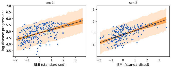
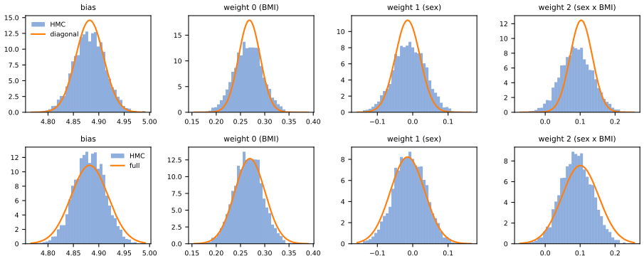
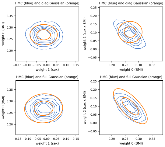
Why the diagonal fit is too narrow here is the result of gap 5.5: for a nearly Gaussian posterior the reverse-KL diagonal variances are the conditional variances \(1/\Lambda_{ii}=\Sigma_{ii}(1-R_i^2)\), where \(R_i^2\) is the squared multiple correlation of coordinate \(i\) with the others; with correlations near \(-0.65\), \(\sqrt{1-0.65^2}=0.76\), which matches the ratios above. The predictive distributions of the two fits are close (the predictive depends mostly on the mean), but statements about individual coefficients are not.
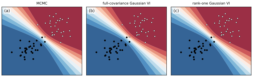
S10.1.2 Full-rank against rank-one Gaussian VI for logistic regression supplement
S10.1.3 Structured (sparse) Gaussian VI supplement
Supp. pp. 126–127 Suppose the energy decomposes over cliques, \(-\log p(\bm z,\mathcal D)=\phi(\bm z)=\sum_c\phi_c(\bm z_c)\) S(10.6). The negative ELBO of \(q=\N(\bm\mu,\bm\Lambda^{-1})\) is \(V=\E_q[\phi]+\frac12\log|\bm\Lambda|\) + const S(10.7). The claim: the optimal precision \(\bm\Lambda\) has the sparsity pattern of the graph, and the natural-gradient updates \[ \bm\Lambda^{i+1}=\E_{q^i}[\nabla^2\phi]=\sum_c\bm P_c^\T\E_{q^i_c}[\nabla^2\phi_c]\bm P_c,\qquad \bm\Lambda^{i+1}\bm\delta^{i+1}=-\E_{q^i}[\nabla\phi],\qquad\bm\mu^{i+1}=\bm\mu^i+\bm\delta^{i+1} \tag{S10.9–S10.11} \] keep it. For a nonlinear least-squares energy \(\phi=\frac12\bm e^\T\bm W^{-1}\bm e\) S(10.12), the Gauss–Newton version replaces the expected Hessian by \(\bar{\bm E}^\T\bm W^{-1}\bar{\bm E}\) S(10.16).
Filling the gap 10.7 supplement: the optimal Gaussian precision inherits the graph's sparsity, and the sign of S(10.17) Supp. pp. 126–127, S(10.6)–S(10.18)
Proof
The supplement's argument ("sparsity maximises entropy") is a heuristic; here is a proof from the stationarity conditions. Assume \(\phi\) is \(C^2\) and \(\nabla\phi,\nabla^2\phi\) have finite expectations under every Gaussian considered.
Gradients of \(V\). By Bonnet's and Price's theorems (gap 6.4), for \(q=\N(\bm\mu,\bm\Sigma)\): \(\nabla_{\bm\mu}\E_q[\phi]=\E_q[\nabla\phi]\) and \(\nabla_{\bm\Sigma}\E_q[\phi]=\frac12\E_q[\nabla^2\phi]\). Also \(\nabla_{\bm\Sigma}(-\frac12\log|\bm\Sigma|)=-\frac12\bm\Sigma^{-1}\). So a stationary point of \(V\) satisfies \[ \E_q[\nabla\phi]=\bm0,\qquad \bm\Lambda=\bm\Sigma^{-1}=\E_q[\nabla^2\phi]. \] Sparsity. \(\nabla^2\phi=\sum_c\bm P_c^\T\nabla^2\phi_c(\bm z_c)\bm P_c\), and the \(c\)-th term is zero outside the rows and columns of the variables in clique \(c\). Hence \((\E_q\nabla^2\phi)_{ij}=0\) unless \(i\) and \(j\) share a clique, i.e. unless \(i=j\) or \((i,j)\) is an edge of the graph. Every stationary point, in particular the optimum, therefore has \(\Lambda_{ij}=0\) for non-adjacent \(i,j\): \(q\) is a Gaussian MRF on the same graph, S(10.8). Numerical confirmation: for a 5-variable chain with non-Gaussian unary terms \(\frac12z^2+0.1z^4\) and pairwise terms \(\frac12(z_i-z_{i+1})^2+0.3\cos(z_i+2z_{i+1})\), optimising the ELBO over a full Cholesky factor (Gauss–Hermite expectations) gives a precision whose entries two or more steps off the diagonal are below \(10^{-4}\) of its largest entry.
The updates S(10.9)–S(10.11) are the fixed-point iteration of these two conditions: set \(\bm\Lambda\) to the current expected Hessian and take a Newton-type step for the mean, \(\bm\mu\leftarrow\bm\mu-\bm\Lambda^{-1}\E_q[\nabla\phi]\). This is the Bayesian learning rule with unit step (gap 6.12), i.e. natural-gradient VI in the Gaussian family; each update is a sum of clique terms, so it has the same sparsity. The marginal covariances \(\bm\Sigma_c\) needed for the clique expectations are blocks of \(\bm\Lambda^{-1}\), not inverses of blocks of \(\bm\Lambda\), which is why the supplement mentions Takahashi's recursions or Gaussian message passing.
Gauss–Newton and the sign of S(10.17). Linearising \(\bm e(\bm z)\approx\bar{\bm e}+\bar{\bm E}(\bm z-\bm\mu)\) and minimising \(\frac12\bm e^\T\bm W^{-1}\bm e\) over the step \(\bm\delta\) gives the normal equations \(\bar{\bm E}^\T\bm W^{-1}\bar{\bm E}\,\bm\delta=-\bar{\bm E}^\T\bm W^{-1}\bar{\bm e}\). The supplement prints S(10.17) without the minus sign; compare S(10.10), which has it. On a three-residual test problem the corrected step lowers the objective and the printed one raises it. \(\square\)
10.2.1.4 Other variational posteriors
p. 449 Many families are reparameterisable (gamma and Dirichlet through implicit reparameterisation gradients; flows, Section 10.4.3).
10.2.1.5 Example: Bayesian parameter inference
pp. 450–451 For a GMM with diagonal precisions, the discrete labels are summed out, \(p(\bm x\given\bm\theta)=\sum_k\pi_k\N(\bm x\given\bm\mu_k,\diag(\bm\lambda_k)^{-1})\) (10.58), and the global posterior is approximated by the mean-field family \(\prod_{k,d}\N(\mu_{kd}\given m_{kd},s_{kd})\Ga(\lambda_{kd}\given\alpha_{kd},\beta_{kd})\cdot\Dir(\bm\pi\given\bm c)\) (10.60), against the prior (10.59) \(\N(0,1)\Ga(5,5)\Dir(\bm1)\). Every factor is reparameterisable, so the ELBO (10.61) is optimised by Algorithm 10.2.
Algorithm 10.2: reparameterised SVI for Bayesian parameter inference
- Initialise \(\bm\psi,\bm\xi\). Repeat:
- sample a minibatch \(\mathcal B\) of size \(B\); sample \(\bm\epsilon\sim q_0\) and set \(\tilde{\bm\theta}=g(\bm\psi,\bm\epsilon)\);
- \(\VFE=-\frac NB\sum_{n\in\mathcal B}\log p(\bm x_n\given\tilde{\bm\theta})-\log p_{\bm\xi}(\tilde{\bm\theta})+\log q_{\bm\psi}(\tilde{\bm\theta})\);
- \(\bm\xi\leftarrow\bm\xi-\eta\nabla_{\bm\xi}\VFE\), \(\bm\psi\leftarrow\bm\psi-\eta\nabla_{\bm\psi}\VFE\); until converged.
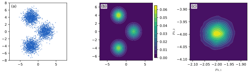
10.2.1.6 Example: MLE for LVMs
p. 452 When the local latents cannot be summed out (variational autoencoders, Section 21.2), an inference network supplies \(q_{\bm\phi}(\bm z_n\given\bm x_n)\):
Algorithm 10.3: reparameterised amortised SVI for the MLE of an LVM
- Initialise \(\bm\theta,\bm\phi\). Repeat: sample \(\bm x_n\sim p_{\mathcal D}\) and \(\bm\epsilon_n\sim q_0\); set \(\bm z_n=g(\bm\phi,\bm x_n,\bm\epsilon_n)\);
- \(\VFE=-\log p_{\bm\theta}(\bm x_n,\bm z_n)+\log q_{\bm\phi}(\bm z_n\given\bm x_n)\); take gradient steps in \(\bm\theta\) and in \(\bm\phi\); until converged.
See also: the deep learning course, Chapter 19 (variational autoencoders).
10.2.2 Automatic differentiation VI
10.2.2.1 Basic idea
pp. 452–453 ADVI (Kucukelbir et al., 2017) maps constrained parameters to \(\R^D\) by a bijection \(T\), \(\bm u=T(\bm\theta)\), puts a Gaussian on \(\bm u\), and uses \(p(\bm u)=p(T^{-1}(\bm u))\,|\det J_{T^{-1}}(\bm u)|\) (10.62), so \[ \ELBO(\bm\psi)=\E_{\bm u\sim q_{\bm\psi}}\big[\log p(\mathcal D\given T^{-1}(\bm u))+\log p(T^{-1}(\bm u))+\log|\det J_{T^{-1}}(\bm u)|\big]+\Hent(\bm\psi). \tag{10.63} \] Deterministic ADVI fixes the draws \(\bm\epsilon_s\) (common random numbers) so that the objective can be optimised with L-BFGS.
Filling the gap 10.8: the Jacobian term, the closed-form entropy, and what fixing the draws does pp. 452–453, (10.62)–(10.63)
Proof
(10.63). The posterior of \(\bm u\) is \(p(\bm u\given\mathcal D)\propto p(\mathcal D\given T^{-1}(\bm u))\,p_{\bm u}(\bm u)\) with the transformed prior (10.62) (change of variables as in gap 10.5). The ELBO for \(q_{\bm\psi}(\bm u)\) is \(\E_q[\log p(\mathcal D,\bm u)]+\Hent(q)\), which is (10.63). By the invariance of KL under bijections (gap 5.2), \(\Dkl(q(\bm u)\|p(\bm u\given\mathcal D))=\Dkl(q_{\bm\theta}\|p(\bm\theta\given\mathcal D))\) where \(q_{\bm\theta}\) is the push-forward of \(q\) by \(T^{-1}\): ADVI is VI with a non-Gaussian family on the original scale. Forgetting the Jacobian targets the wrong density (the posterior "density" in \(\bm\theta\) evaluated at \(T^{-1}(\bm u)\)). For \(q=\N(\bm\mu,\bm\Sigma)\), \(\Hent=\frac12\log\det(2\pi e\bm\Sigma)\), so only the first expectation needs Monte Carlo.
The examples' Jacobians. For \(\theta=\sigm(z)\): \(\d\theta/\d z=\sigm(z)\sigm(-z)\), \(\log|J|=\log\sigm(z)+\log\sigm(-z)\). For the supplement's \(\sigma=10\,\sigm(\tau)\): \(\log|J|=\log10+\log\sigm(\tau)+\log\sigm(-\tau)\), and the uniform prior contributes \(-\log10\). Beta-binomial (Section 10.2.2.2). With \(N_1=10\), \(N_0=1\), \(a=b=1\), the posterior is \(\mathrm{Beta}(11,2)\); maximising (10.63) by quadrature gives an ELBO of \(\log B(11,2)-0.022\), i.e. \(\Dkl(q\|p)=0.022\) nats: the logit Gaussian is a good fit despite the skew, as the book says (compare the posterior approximations demo of Chapter 7).
Fixed draws. With \(\bm\epsilon_1,\dots,\bm\epsilon_S\) fixed, \(\hat\ELBO_S(\bm\psi)=\frac1S\sum_sf(g(\bm\psi,\bm\epsilon_s))+\Hent(\bm\psi)\) is a deterministic smooth function (sample-average approximation). Its maximiser is not the ELBO maximiser for finite \(S\), but under a uniform law of large numbers on compact parameter sets (e.g. \(f\circ g\) continuous in \(\bm\psi\) and dominated by an integrable envelope) \(\hat\ELBO_S\to\ELBO\) uniformly almost surely, and the maximisers converge when the ELBO maximiser is unique (the standard argmax-consistency argument). For Figure 10.2 with 20 000 fixed draws the full and low-rank fits have KL below \(10^{-3}\) from the exact posterior. \(\square\)
10.2.2.2 Example: ADVI for beta-binomial model
p. 453 Computed in gap 10.8 above; the figure is Figure 7.4, reproduced in Section 7.4.4 of these notes.
10.2.2.3 Example: ADVI for GMMs
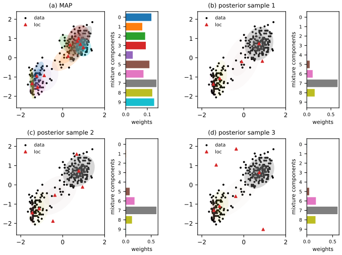
pp. 453–454 The labels are summed out (10.64) and a Gaussian is placed on all the unconstrained parameters of a \(K=10\) component mixture fitted to Old Faithful. Setting the covariance to zero gives a MAP fit, which has no Occam factor and uses every component.
10.2.2.4 More complex posteriors
p. 453 ADVI combines with mixtures or flows on \(\bm u\) (Section 10.4).
10.2.3 Blackbox variational inference
10.2.3.1 Estimating the gradient using REINFORCE
pp. 454–455 When \(\tilde L(\bm\psi,\bm z)=\log p(\bm x,\bm z)-\log q(\bm z\given\bm\psi)\) can be evaluated but not differentiated in \(\bm z\) (discrete \(\bm z\), say), use \[ \nabla_{\bm\psi}\ELBO(\bm\psi)=\E_{q(\bm z|\bm\psi)}\big[\tilde L(\bm\psi,\bm z)\,\nabla_{\bm\psi}\log q(\bm z\given\bm\psi)\big]\approx\frac1S\sum_{s=1}^S\tilde L(\bm\psi,\bm z_s)\nabla_{\bm\psi}\log q(\bm z_s\given\bm\psi): \tag{10.66, 10.67} \] blackbox VI (Ranganath et al., 2014).
10.2.3.2 Reducing the variance using control variates
p. 455 For component \(i\), with \(g_i=\partial_{\psi_i}\log q\) and \(\tilde g_i=g_i\tilde L\), replace \(\tilde g_i\) by \(\tilde g_i+c_i(\E[b_i]-b_i)\) (10.71). The score itself is a convenient baseline, \(b_i=g_i\), \(\E[g_i]=0\), giving \(g_i(\tilde L-c_i)\) (10.72)–(10.73), and the best constant is \[ c_i=\frac{\cov\big(g_i\tilde L,\ g_i\big)}{\var(g_i)}. \tag{10.74} \]
Filling the gap 10.9: (10.66) holds although \(\tilde L\) depends on \(\bm\psi\); the optimal constant (10.74) and the variance it removes pp. 454–455, (10.65)–(10.74)
Proof
(10.66). By gap 10.4 (same domination conditions), \(\nabla_{\bm\psi}\E_q[\tilde L]=\E_q[\tilde L\nabla\log q]+\E_q[\nabla_{\bm\psi}\tilde L]\). But \(\nabla_{\bm\psi}\tilde L(\bm\psi,\bm z)=-\nabla_{\bm\psi}\log q(\bm z\given\bm\psi)\), and the score has mean zero: \(\E_q[\nabla\log q]=\int\nabla q\,\d\bm z=\nabla\int q\,\d\bm z=\nabla1=\bm0\) (the score identity, Section 3.3; for discrete \(\bm z\) replace the integral by a sum). So the second term vanishes and (10.66) is exact. The general estimator and its variance are in gap 6.3.
Control variate. For any constant \(c\), \(\E[g_i(\tilde L-c)]=\E[g_i\tilde L]-c\,\E[g_i]=\E[g_i\tilde L]\): unbiased. Its variance is \(v(c)=\var(\tilde g_i)-2c\cov(\tilde g_i,g_i)+c^2\var(g_i)\), a convex quadratic in \(c\) minimised at \(c^*=\cov(\tilde g_i,g_i)/\var(g_i)\), which is (10.74), with minimum \(v(c^*)=\var(\tilde g_i)(1-\rho^2)\), \(\rho=\operatorname{corr}(\tilde g_i,g_i)\). Since \(\E[g_i]=0\), \(c^*=\E[g_i^2\tilde L]/\E[g_i^2]\): a score-weighted average of \(\tilde L\). Estimating \(c^*\) from the same \(S\) draws makes the estimator slightly biased (of order \(1/S\)); using \(c\) from the previous iteration or a separate pilot run keeps it unbiased.
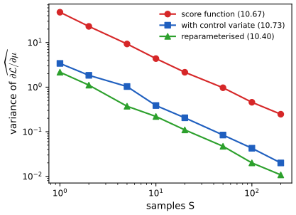
Why it matters. \(\tilde L\) contains constants (normalisers of \(p\) and \(q\)) that carry no information about the gradient but multiply the zero-mean score: with \(\tilde L=k+\ell(\bm z)\) the naive estimator has an extra variance \(k^2\var(g_i)\) that the control variate removes (practice problem 10.3 works this out exactly for a Gaussian). In Figure 10.x1, for a Poisson count model with a Gaussian prior on the log rate (\(q=\N(0.5,0.5^2)\)), the pilot estimate is \(c^*\approx-3.2\) and the variance of the \(\mu\) gradient falls from 47.8 to 3.4 with \(S=1\), close to the reparameterised estimator's 2.2. \(\square\)
Online variational inference supplement 10.2
Supp. pp. 128–130 Streaming variational Bayes (Broderick et al., 2013), also variational continual learning: at step \(t\) the previous posterior is the prior, \[ \bm\psi_t=\argmin_{\bm\psi}\ \E_{q(\bm\theta|\bm\psi)}[\ell_t(\bm\theta)]+\Dkl\big(q(\bm\theta\given\bm\psi)\,\|\,q(\bm\theta\given\bm\psi_{t-1})\big),\qquad\ell_t=-\log p(\mathcal D_t\given\bm\theta). \tag{S10.19} \] FOO-VB (Zeno et al., 2021) uses Gaussians, \(q(\cdot\given\bm\psi_t)=\N(\bm\mu,\bm\Sigma)\), \(q(\cdot\given\bm\psi_{t-1})=\N(\bm m,\bm V)\), \(\bm\Sigma=\bm L\bm L^\T\), and solves the stationarity conditions S(10.27)–S(10.30) with the expectations evaluated at the previous parameters, which gives a one-step update. In the diagonal case this is Bayesian gradient descent (supplement Algorithm 10.1): with \(E_{1i}=\E[g_i]\), \(E_{2i}=\E[g_i\epsilon_i]\) estimated from \(K\) draws \(\bm\theta_k=\bm\mu_{t-1}+\bm\sigma_{t-1}\odot\bm\epsilon_k\), \[ \mu_{t,i}=\mu_{t-1,i}-\sigma_{t-1,i}^2E_{1i},\qquad \sigma_{t,i}=\sigma_{t-1,i}\sqrt{1+\big(\tfrac12\sigma_{t-1,i}E_{2i}\big)^2}-\tfrac12\sigma_{t-1,i}^2E_{2i}. \tag{S10.35} \]
Filling the gap 10.10 supplement: the FOO-VB stationarity conditions, the root S(10.34)–S(10.35), and when the one-step iteration converges Supp. pp. 128–130, S(10.19)–S(10.35)
Proof
The objective. By the Gaussian KL formula (Volume 1, Result 6.3), the quantity minimised in S(10.19) is \[ J(\bm\mu,\bm L)=\tfrac12\Big[\log\tfrac{|\bm V|}{|\bm\Sigma|}-D+\Tr(\bm V^{-1}\bm\Sigma)+(\bm m-\bm\mu)^\T\bm V^{-1}(\bm m-\bm\mu)\Big]+\E_{q}[\ell_t(\bm\theta)], \] which is S(10.22). (The supplement names it \(\ELBO_t\), but it is the negative ELBO, \(-\ELBO_t\) in S(10.19).)
Derivatives. \(\partial\Tr(\bm V^{-1}\bm L\bm L^\T)/\partial\bm L=2\bm V^{-1}\bm L\) (S(10.23), using symmetry of \(\bm V^{-1}\)); \(-\frac12\log|\bm\Sigma|=-\log|\det\bm L|\) and \(\partial\log|\det\bm L|/\partial\bm L=\bm L^{-\T}\) (S(10.24), Jacobi's formula). With \(\bm\theta=\bm\mu+\bm L\bm\epsilon\), \(\partial\E_{\bm\epsilon}[\ell_t]/\partial L_{ij}=\E[\partial_i\ell_t\,\epsilon_j]\) (S(10.26), differentiating under the integral). Setting the gradients to zero: \(-\bm V^{-1}(\bm m-\bm\mu)+\E[\nabla\ell_t]=\bm0\) (S(10.27)), and \(-\bm L^{-\T}+\bm V^{-1}\bm L+\E[\nabla\ell_t\,\bm\epsilon^\T]=\bm0\) (S(10.30)).
Diagonal case. With \(\bm L=\diag(\sigma_i)\), \(\bm V=\diag(v_i^2)\), coordinate \(i\) of S(10.30) is \(-1/\sigma_i+\sigma_i/v_i^2+E_{2i}=0\); multiplying by \(\sigma_i>0\): \(\sigma_i^2/v_i^2+E_{2i}\sigma_i-1=0\) (S(10.33)). The product of the roots is \(-v_i^2<0\), so exactly one root is positive, \(\sigma_i=\frac{v_i^2}2\big(-E_{2i}+\sqrt{E_{2i}^2+4/v_i^2}\big)=-\frac12v_i^2E_{2i}+v_i\sqrt{1+(\frac12v_iE_{2i})^2}\) (S(10.34)–S(10.35)). By Stein's lemma \(E_{2i}=\E[\partial_i\ell(\bm\mu+\bm\sigma\odot\bm\epsilon)\epsilon_i]=\sigma_i\E[\partial^2_{ii}\ell]\), so the root solves \(1/\sigma_i^2=1/v_i^2+\E[\partial_{ii}^2\ell]\): new precision = old precision + expected curvature, the Gaussian analogue of Bayes' rule.
Convergence. For a quadratic loss \(\ell=\frac a2(\theta-b)^2\) in one dimension the conditions are solved exactly by the conjugate posterior (precision \(1/v^2+a\), mean \((m/v^2+ab)/(1/v^2+a)\)), confirmed numerically. Iterating the mean condition with the expectation at the previous mean, \(\mu\leftarrow m-v^2a(\mu-b)\), is a linear map with slope \(-v^2a\): it converges iff \(v^2a<1\) and diverges otherwise (confirmed with \(v^2a=2\)). This is why BGD adds a learning rate \(\eta\) to the mean step S(10.31). \(\square\)
10.3 Coordinate ascent VI
pp. 455–456 The mean-field family \(q(\bm z)=\prod_{j=1}^Jq_j(\bm z_j)\) (10.75) turns the ELBO into \[ \ELBO(\bm\psi)=\int q(\bm z)\log p_{\bm\theta}(\bm x,\bm z)\d\bm z+\sum_{j=1}^J\Hent(q_j), \tag{10.76} \] since the entropy of a product is the sum of the entropies (\(\log\prod_jq_j=\sum_j\log q_j\), and \(\E_q\log q_j=\E_{q_j}\log q_j\)). The first term often decomposes along the graph, which makes coordinate ascent (CAVI) natural.
10.3.1 Derivation of CAVI algorithm
pp. 456–457 Holding all factors but \(q_j\) fixed, the ELBO is \(\E_{q_j}[g_j(\bm z_j)-\log q_j(\bm z_j)]\)+const with \(g_j(\bm z_j)=\E_{\bm z_{-j}}[\log\tilde p(\bm z)]\) (10.80), which is \(-\Dkl(q_j\|f_j)\)+const for the normalised \(f_j\propto\exp(g_j)\) (10.81)–(10.83), so the optimum is \[ q_j(\bm z_j)\propto\exp\Big[\E_{\bm z_{{\rm mb}_j}}\log\tilde p(\bm z_j,\bm z_{{\rm mb}_j})\Big], \tag{10.87} \] where only the Markov blanket of \(\bm z_j\) matters. Compare the Gibbs sampling conditional: CAVI replaces sampling the blanket by averaging over it.
Algorithm 10.4: coordinate ascent variational inference (CAVI)
- Initialise \(q_j(\bm z_j)\), \(j=1{:}J\).
- For \(t=1{:}T\), for \(j=1{:}J\): compute \(g_j(\bm z_j)=\E_{\bm z_{{\rm mb}_j}}[\log\tilde p(\bm z_j,\bm z_{{\rm mb}_j})]\) and set \(q_j\propto\exp(g_j)\).
Filling the gap 10.11: the CAVI update for general variables, the Markov blanket, and what "convergence is guaranteed" means pp. 456–457, (10.77)–(10.87)
Proof
The book derives (10.83) for three discrete variables; the general argument (continuous or discrete, any \(J\)) is in the Bishop course, gap 10.2: if \(g_j\) is finite \(q_{-j}\)-almost surely and \(Z_j=\int e^{g_j}\d\bm z_j<\infty\), then \(\ELBO=-\Dkl(q_j\|f_j)+\log Z_j\)+terms not involving \(q_j\), so \(f_j\) is the unique maximiser over all densities \(q_j\). Three points the book leaves implicit:
Markov blanket (10.84)–(10.87). Write \(\log\tilde p(\bm z)=\sum_c\log\psi_c(\bm z_c)\) over the factors of the graph. Factors not containing \(\bm z_j\) contribute a constant to \(g_j\) (their expectation does not depend on \(\bm z_j\)); the factors containing \(\bm z_j\) involve only \(\bm z_j\) and its neighbours in the factor graph, which is its Markov blanket. So \(g_j\) needs only the marginals \(q_k\) of the blanket.
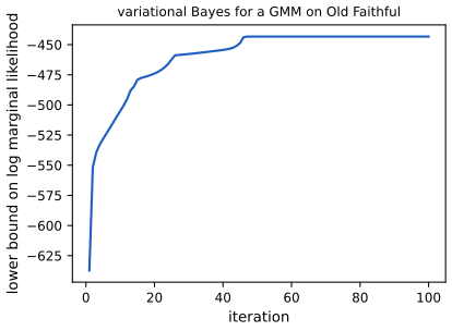
Monotonicity. Each update maximises \(\ELBO\) exactly over \(q_j\) with the others fixed, so the sequence of ELBO values is non-decreasing; it is bounded above by \(\log p(\bm x)\) and therefore converges. This is the precise content of "convergence is guaranteed": the objective converges. As a functional of \(q_j\) alone the ELBO is concave (linear term plus entropy), but it is not jointly concave in \((q_1,\dots,q_J)\), so the limit may be a local optimum that depends on the initialisation and the update order (Section 10.3.6 and Supplement 10.4.2 give examples).
Sequential, not parallel. The argument needs the factors to be updated one at a time with the newest values of the others. Updating all factors simultaneously from the old values is not coordinate ascent and can decrease the ELBO or oscillate; see gap 10.12. \(\square\)
10.3.2 Example: CAVI for the Ising model
pp. 458–459 Binary pixels \(z_i\in\{-1,+1\}\) on a grid with an Ising prior \(p(\bm z)\propto\exp(\sum_{i\sim j}W_{ij}z_iz_j)\) (10.89)–(10.90) and local evidence \(L_i(z_i)=\log p(x_i\given z_i)\) (10.88). With the fully factorised \(q(\bm z)=\prod_i\Ber(z_i\given\mu_i)\) (10.93), \(\mu_i=\E_{q_i}[z_i]\), the update is \[ q_i(z_i=1)=\sigm(2a_i),\qquad a_i=m_i+\tfrac12(L_i^+-L_i^-),\qquad m_i=\sum_{j\in{\rm nbr}_i}W_{ij}\mu_j,\qquad \mu_i=\tanh(a_i), \tag{10.96–10.99} \] used as a fixed-point iteration, optionally damped: \[ \mu_i^t=(1-\lambda)\mu_i^{t-1}+\lambda\tanh\Big(\sum_{j\in{\rm nbr}_i}W_{ij}\mu_j^{t-1}+\tfrac12(L_i^+-L_i^-)\Big). \tag{10.101} \]
Filling the gap 10.12: the Ising updates, the mean-field ELBO, and why parallel updates need damping pp. 458–459, (10.88)–(10.101)
Proof
The update. The terms of \(\log\tilde p(\bm z)=\sum_{i\sim j}W_{ij}z_iz_j+\sum_iL_i(z_i)\) containing \(z_i\) are \(z_i\sum_{j\in{\rm nbr}_i}W_{ij}z_j+L_i(z_i)\) (10.94). Averaging over the other factors (independent under \(q\)) replaces \(z_j\) by \(\mu_j\) (10.95), so \(q_i(z_i)\propto e^{z_im_i+L_i(z_i)}\). Hence \(q_i(+1)=e^{m_i+L_i^+}/(e^{m_i+L_i^+}+e^{-m_i+L_i^-})=1/(1+e^{-2a_i})=\sigm(2a_i)\), and \(\mu_i=\sigm(2a_i)-\sigm(-2a_i)=\frac{e^{a_i}-e^{-a_i}}{e^{a_i}+e^{-a_i}}=\tanh a_i\). For Gaussian evidence \(x_i\given z_i\sim\N(z_i,\sigma^2)\), \(\frac12(L_i^+-L_i^-)=\frac{(x_i+1)^2-(x_i-1)^2}{4\sigma^2}=x_i/\sigma^2\).
The objective. With \(p_i=(1+\mu_i)/2=q_i(+1)\), independence gives \(\E_q[z_iz_j]=\mu_i\mu_j\), so \[ \ELBO(\bm\mu)=\sum_{i\sim j}W_{ij}\mu_i\mu_j+\sum_i\big[p_iL_i^++(1-p_i)L_i^-\big]+\sum_i\Hent_b(p_i)-\log Z_0, \] with \(\Hent_b\) the binary entropy. Its partial derivative in \(\mu_i\) is \(m_i+\frac12(L_i^+-L_i^-)-\operatorname{artanh}\mu_i\) (using \(\partial_{\mu}\Hent_b((1+\mu)/2)=-\frac12\log\frac{1+\mu}{1-\mu}=-\operatorname{artanh}\mu\)), and the second derivative \(-1/(1-\mu_i^2)<0\): the ELBO is strictly concave in each \(\mu_i\) and maximised at \(\mu_i=\tanh(a_i)\). A grid search over \(\mu_i\) on the denoising problem lands on the tanh value to \(10^{-3}\).
Parallel updates. Sequential updates are coordinate ascent and never decrease the ELBO (gap 10.11). The parallel ("Jacobi") update sets every \(\mu_i\) from the old neighbours. On a bipartite graph such as a grid, the even and odd sublattices then drive each other: a pattern \(\mu\) on one sublattice produces the response on the other, which produces the response back, and when the coupling \(W\) is large enough the map has a stable 2-cycle, the checkerboard. In a linearisation around a fixed point, \(\bm\mu\mapsto\bm D\bm W\bm\mu\) with \(\bm D=\diag(1-\mu_i^2)\); the eigenvalues of a bipartite \(\bm W\) come in pairs \(\pm\kappa\), and an eigenvalue below \(-1\) makes the undamped iteration flip sign at every step. Damping (10.101) maps each eigenvalue \(e\) to \(1-\lambda+\lambda e\); with \(\lambda=\frac12\) an eigenvalue \(e\ge-3\) becomes \(\ge-1\), removing the oscillation in the regimes met in practice. In the denoising run of Figure 10.9 (64×64 image, \(W=1\), \(\sigma=2\)), between sweeps 14 and 15 the undamped parallel scheme still flips the sign of 4.2% of the pixels, the damped one 0.2%, the sequential one 0.07%; after 15 sweeps the ELBOs are \(-1564\) (undamped parallel), \(-1227\) (damped parallel) and \(-1172\) (sequential). \(\square\)
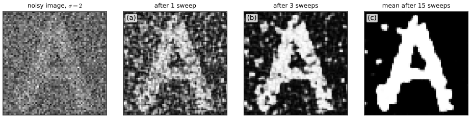
See also: Section 4.3.2 (Ising models) and the Ising and Potts demo.
10.3.3 Variational Bayes
pp. 459–460 Treating the parameters as the latent variables, \(p(\bm\theta,\mathcal D)=p(\bm\theta)\prod_np(\mathcal D_n\given\bm\theta)\) (10.102), and maximising \(\E_q[\log p(\bm\theta,\mathcal D)]+\Hent(q)\) (10.103) over a factorised \(q(\bm\theta)=\prod_jq(\bm\theta_j)\) (10.104) by CAVI is variational Bayes.
10.3.4 Example: VB for a univariate Gaussian
pp. 460–463 Likelihood \(\prod_n\N(x_n\given\mu,\lambda^{-1})\), conjugate prior \(\N(\mu\given\mu_0,(\kappa_0\lambda)^{-1})\Ga(\lambda\given a_0,b_0)\) (10.105), factorised \(q(\mu)q(\lambda)\) (10.106). The optimal factors are \(q(\mu)=\N(\mu\given\mu_N,\kappa_N^{-1})\) and \(q(\lambda)=\Ga(\lambda\given a_N,b_N)\) with \[ \mu_N=\frac{\kappa_0\mu_0+N\bar x}{\kappa_0+N},\quad \kappa_N=(\kappa_0+N)\frac{a_N}{b_N},\quad a_N=a_0+\frac{N+1}2,\quad b_N=b_0+\tfrac12\kappa_0\big(\E\mu^2+\mu_0^2-2\E\mu\,\mu_0\big)+\tfrac12\sum_n\big(x_n^2+\E\mu^2-2\E\mu\,x_n\big), \tag{10.119–10.122} \] derived in full in the Bishop course, gaps 10.3–10.5 (with Bishop's \(\tau\) for \(\lambda\)). Only \(\kappa_N\) and \(b_N\) change between iterations. The bound has the simple form \[ \ELBO=\const+\tfrac12\log\frac1{\kappa_N}+\log\Gamma(a_N)-a_N\log b_N. \tag{10.124} \]
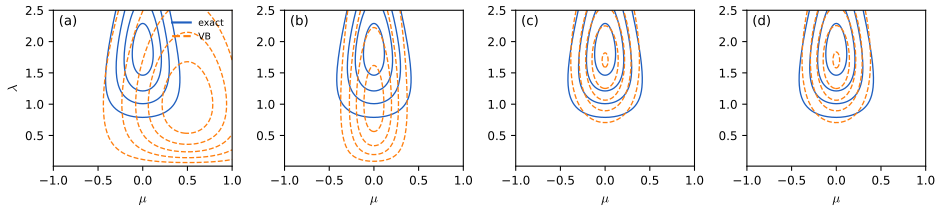
See also: the VB Gaussian demo of the Bishop course.
Filling the gap 10.13: the fixed point in closed form, what VB gets right and wrong, and the bound (10.124) pp. 461–463, (10.119)–(10.124)
Proof
Fixed point. Put \(c_0=b_0+\frac12\kappa_0(\mu_N-\mu_0)^2+\frac12\sum_n(x_n-\mu_N)^2\). Using \(\E\mu^2=\mu_N^2+1/\kappa_N\) in (10.122), \(b_N=c_0+\frac{\kappa_0+N}{2\kappa_N}\), and (10.120) gives \(\frac{\kappa_0+N}{\kappa_N}=\frac{b_N}{a_N}\). Hence \(b_N=c_0+\frac{b_N}{2a_N}\), i.e. \[ b_N=\frac{c_0}{1-1/(2a_N)},\qquad \E_q[\lambda]=\frac{a_N}{b_N}=\frac{a_N-\frac12}{c_0}=\frac{a_0+N/2}{c_0},\qquad \kappa_N=(\kappa_0+N)\frac{a_0+N/2}{c_0}. \] This is the analytic solution the book mentions (the iteration converges to it; for the data of Figure 10.10, \(b_N=3.228560\) both ways).
Comparison with the exact posterior. The exact posterior is \(\N(\mu\given\mu_N,(\kappa_{\rm ex}\lambda)^{-1})\Ga(\lambda\given a_{\rm ex},b_{\rm ex})\) with \(\kappa_{\rm ex}=\kappa_0+N\), \(a_{\rm ex}=a_0+N/2\), \(b_{\rm ex}=b_0+\frac12\sum(x_n-\bar x)^2+\frac{\kappa_0N(\bar x-\mu_0)^2}{2(\kappa_0+N)}\) (Section 3.4.3.3). Since \(\sum(x_n-\mu_N)^2=\sum(x_n-\bar x)^2+N(\bar x-\mu_N)^2\) and \(\kappa_0(\mu_N-\mu_0)^2+N(\bar x-\mu_N)^2=\frac{\kappa_0N}{\kappa_0+N}(\bar x-\mu_0)^2\), we get \(c_0=b_{\rm ex}\). Consequences: (i) VB's mean of \(\mu\) and its \(\E[\lambda]=a_{\rm ex}/b_{\rm ex}\) are exactly the posterior ones; (ii) VB's variance of \(\mu\) is \(1/\kappa_N=\frac{b_{\rm ex}}{\kappa_{\rm ex}a_{\rm ex}}\), while the exact marginal of \(\mu\) is a Student \(t\) with variance \(\frac{b_{\rm ex}}{\kappa_{\rm ex}(a_{\rm ex}-1)}\): VB is too small by the factor \((a_{\rm ex}-1)/a_{\rm ex}\) (5/6 in Figure 10.10: 0.0452 against 0.0542); (iii) VB's variance of \(\lambda\) is too small by \(a_{\rm ex}/(a_{\rm ex}+\frac12)\). Both errors vanish as \(N\to\infty\).
The bound (10.124). Write \(Q(\mu)=\kappa_0(\mu-\mu_0)^2+\sum_n(x_n-\mu)^2\). The log joint (10.108) is \((a_0-1+\frac{N+1}2)\log\lambda-\lambda(b_0+\frac12Q(\mu))\)+const, so \(\E_q[\log p]=(a_N-1)\E\log\lambda-\E\lambda\,(b_0+\frac12\E Q)\)+const. Right after a \(q(\lambda)\) update, \(b_N=b_0+\frac12\E Q\) by (10.122), so this is \((a_N-1)\E\log\lambda-b_N\E\lambda\)+const. Subtract \(\E\log q(\lambda)=(a_N-1)\E\log\lambda-b_N\E\lambda+a_N\log b_N-\log\Gamma(a_N)\) and \(\E\log q(\mu)=\frac12\log\kappa_N-\frac12\log2\pi-\frac12\): the \(\lambda\) terms cancel and \[ \ELBO=\Big[-\tfrac N2\log2\pi+\tfrac12\log\kappa_0+a_0\log b_0-\log\Gamma(a_0)+\tfrac12\Big]+\tfrac12\log\frac1{\kappa_N}+\log\Gamma(a_N)-a_N\log b_N. \] The bracket is the constant of (10.124). The formula equals the exact ELBO to \(10^{-10}\) after every \(q(\lambda)\) update of the run; the exact ELBO rises at every half step and stays below the exact log evidence (\(-12.194\) against \(-12.153\) here, a gap of 0.041 nats). (With the improper prior \(\kappa_0=a_0=b_0=0\) the constant is \(-\infty\), which is why a proper prior is used for the numbers.) \(\square\)
10.3.5 Variational Bayes EM
pp. 463–464 With local latents \(\bm z_n\) and global parameters \(\bm\theta\), \(p(\bm\theta,\bm z_{1:N},\mathcal D)=p(\bm\theta)\prod_np(\bm z_n\given\bm\theta)p(\bm x_n\given\bm z_n,\bm\theta)\) (10.125), the mean-field family \(q(\bm\theta)\prod_nq(\bm z_n)\) (10.126) and CAVI give VBEM: a variational E step averaging over \(\bm\theta\), a variational M step updating the parameter posterior from expected sufficient statistics. Restricting \(q(\bm\theta)\) to a point mass gives variational EM (VEM) with objective (10.128).
Filling the gap 10.14: the point-mass limit that turns VBEM into VEM p. 464, (10.127)–(10.128)
Proof
A point mass has no density, and the entropy of \(\N(\hat{\bm\theta},s^2\bm I)\) tends to \(-\infty\) as \(s\to0\), so (10.128) is not literally (10.127) at \(q(\bm\theta)=\delta\). The correct statement: for \(q_s(\bm\theta)=\N(\hat{\bm\theta},s^2\bm I)\) and \(\bm\theta\mapsto\log p(\bm\theta,\mathcal D,\bm z)\) continuous and suitably bounded near \(\hat{\bm\theta}\), \[ \ELBO(q_s\textstyle\prod_nq_n)-\Hent(q_s)\ \longrightarrow\ \E_{\prod q_n}\big[\log p(\hat{\bm\theta},\mathcal D,\bm z_{1:N})-\log\prod_nq_n(\bm z_n)\big]\quad(s\to0), \] by dominated convergence. The right side is (10.128): VEM maximises the VBEM objective without the parameter entropy, i.e. it maximises \(\log p(\hat{\bm\theta})+\)(a lower bound on \(\log p(\mathcal D\given\hat{\bm\theta})\)), a MAP version of variational EM. Dropping \(\Hent(q(\bm\theta))\) is exactly what removes the Occam factor that makes VBEM prune components (Section 10.3.6.4). \(\square\)
10.3.6 Example: VBEM for a GMM
pp. 464–467 For a GMM (10.129) with conjugate prior \(\Dir(\bm\pi\given\breve{\bm\alpha})\prod_k\N(\bm\mu_k\given\breve{\bm m},(\breve\kappa\bm\Lambda_k)^{-1})\Wi(\bm\Lambda_k\given\breve{\bm L},\breve\nu)\) (10.130), the exact posterior is a mixture over all \(K^N\) labellings. The mean-field optimum is \(q_n(\bm z_n)=\Cat(\bm z_n\given\bm r_n)\) (10.131) and \(q(\bm\theta)=\Dir(\bm\pi\given\hat{\bm\alpha})\prod_k\N(\bm\mu_k\given\hat{\bm m}_k,(\hat\kappa_k\bm\Lambda_k)^{-1})\Wi(\bm\Lambda_k\given\hat{\bm L}_k,\hat\nu_k)\) (10.132), with the M step (10.137)–(10.145) (counts \(N_k=\sum_nr_{nk}\), means \(\bar{\bm x}_k\), scatter \(\bm S_k\)) and an E step built from three expectations: \[ \E[\log\pi_k]=\dg(\hat\alpha_k)-\dg\Big(\sum_{k'}\hat\alpha_{k'}\Big),\quad \E\log|\bm\Lambda_k|=\sum_{j=1}^D\dg\Big(\frac{\hat\nu_k+1-j}2\Big)+D\log2+\log|\hat{\bm L}_k|,\quad \E\big[(\bm x_n-\bm\mu_k)^\T\bm\Lambda_k(\bm x_n-\bm\mu_k)\big]=\frac D{\hat\kappa_k}+\hat\nu_k(\bm x_n-\hat{\bm m}_k)^\T\hat{\bm L}_k(\bm x_n-\hat{\bm m}_k), \tag{10.147, 10.149, 10.150} \] so that \(r_{nk}\propto\tilde\pi_k\tilde\Lambda_k^{1/2}\exp\big(-\frac D{2\hat\kappa_k}-\frac{\hat\nu_k}2(\bm x_n-\hat{\bm m}_k)^\T\hat{\bm L}_k(\bm x_n-\hat{\bm m}_k)\big)\) (10.151) with \(\tilde\pi_k=e^{\E\log\pi_k}\), \(\tilde\Lambda_k=e^{\E\log|\bm\Lambda_k|}\). All of these are derived in the Bishop course, gaps 10.6–10.9, and confirmed here by Monte Carlo (Dirichlet and Wishart draws reproduce the three expectations to two decimals). Note that the book uses \(\tilde\Lambda_k\) in (10.150) for the expected quadratic form and in (10.151) for \(e^{\E\log|\bm\Lambda_k|}\); the formula above uses the second meaning.
10.3.6.4 Automatic sparsity inducing effects of VBEM
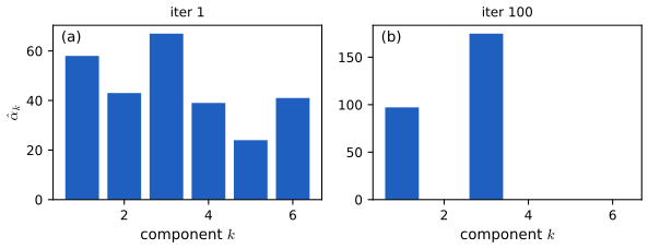
pp. 467–468 Ignoring the likelihood, VBEM sets \(r_{nk}\propto\tilde\pi_k=e^{\dg(\hat\alpha_k)}/e^{\dg(\sum\hat\alpha_{k'})}\) (10.153), where EM-MAP sets \(r_{nk}=\hat\pi_k=(\hat\alpha_k-1)/\sum_{k'}(\hat\alpha_{k'}-1)\) (10.154). With \(\alpha_0=0\) (10.155)–(10.156) an empty cluster gets a negative EM weight but a zero VB weight, and small clusters are shrunk more than large ones.
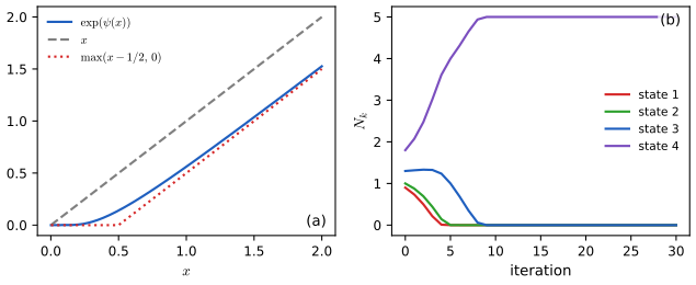
Filling the gap 10.15: \(e^{\dg(x)}<x\), the soft threshold, and a proof of "rich get richer" pp. 467–468, (10.153)–(10.156)
Proof
Digamma as an expected log. For \(x>0\), \(\Gamma(x)=\int_0^\infty t^{x-1}e^{-t}\d t\) can be differentiated under the integral (the integrand's \(x\)-derivative \(t^{x-1}e^{-t}\log t\) is dominated locally uniformly), so \(\Gamma'(x)=\int\log t\,t^{x-1}e^{-t}\d t\) and \(\dg(x)=\Gamma'(x)/\Gamma(x)=\E[\log G]\) for \(G\sim\Ga(x,1)\). By Jensen's inequality, strict because \(G\) is not constant, \(\dg(x)<\log\E G=\log x\): \(e^{\dg(x)}<x\) for every \(x>0\). (The Monte Carlo average of \(\log G\) for \(x=2.7\) matches \(\dg(2.7)\) to 0.005.)
The two ends. From \(\dg(x+1)=\dg(x)+1/x\) (differentiate \(\log\Gamma(x+1)=\log x+\log\Gamma(x)\)), \(\dg(x)=-1/x-\gamma+O(x)\) as \(x\to0\), so \(e^{\dg(x)}\approx e^{-\gamma}e^{-1/x}\) vanishes faster than any power: tiny counts are set essentially to zero (never exactly). For large \(x\), Stirling's series gives \(\dg(x)=\log x-\frac1{2x}-\frac1{12x^2}+O(x^{-4})\), hence \(e^{\dg(x)}=x-\frac12+\frac1{24x}+O(x^{-2})\): large counts lose about one half. The lower bound \(e^{\dg(x)}>x-\frac12\) for \(x\ge\frac12\) shown in Figure 10.11a was confirmed numerically on \([\frac12,50]\).
The book's remark that the digamma function "is always positive" is not right: \(\dg(1)=-\gamma=-0.577\) and \(\dg(x)<0\) for \(x<1.4616\). What is always positive is \(e^{\dg(x)}\), which is what keeps the VB weights non-negative.
Rich get richer. Let \(r(x)=e^{\dg(x)}/x\). Then \((\log r)'=\dg'(x)-\frac1x\), and \(\dg'(x)=\sum_{n\ge0}(x+n)^{-2}>\int_0^\infty(x+t)^{-2}\d t=\frac1x\) (the summand is decreasing in \(n\), so each term exceeds the integral over \([n,n+1]\)). So \(r\) is strictly increasing. With \(\alpha_0=0\) and no likelihood, one update maps \(N_k\mapsto c\,N_kr(N_k)\) with the same \(c\) for all \(k\), hence for \(N_k>N_j\): \[ \frac{N_k^{\rm new}}{N_j^{\rm new}}=\frac{N_k}{N_j}\cdot\frac{r(N_k)}{r(N_j)}>\frac{N_k}{N_j}. \] Every ratio of a larger to a smaller count grows at every step; the total \(N\) is preserved, so the largest count increases and the smallest decreases: the largest cluster eventually takes everything, as in Figure 10.11b (after 30 steps the three small counts are below \(10^{-40}\)). The likelihood counteracts this whenever the data really need several clusters, which is why only the redundant components are pruned. \(\square\)
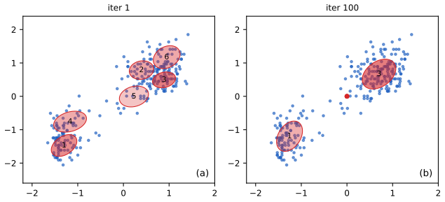
p. 468 On Old Faithful with \(K=6\), \(\alpha_0=0.001\) and a K-means start, four components are switched off:
10.3.6.5 Lower bound on the marginal likelihood
p. 468 VBEM maximises \(\sum_{\bm z}\int q\log\frac{p(\bm x,\bm z,\bm\theta)}{q}\d\bm\theta\le\log p(\bm x)\) (10.157), which never decreases (gap 10.11). I compute it with the seven-term formula of Bishop (2006, (10.70)–(10.77)), after each M step.
See also: the variational mixture of Gaussians demo (Bishop course).
10.3.6.6 Model selection using VBEM
p. 470 Fitting several \(K\) and using \(p(K\given\mathcal D)\approx e^{\ELBO(K)}/\sum_{K'}e^{\ELBO(K')}\) (10.158) needs a correction for label switching: \(\log p(\mathcal D\given K)\approx\ELBO(K)+\log K!\).
Filling the gap 10.16: where \(\log K!\) comes from, and when it over-corrects p. 470
Proof
The likelihood and a symmetric prior are invariant under the \(K!\) relabellings \(\sigma\) of the components, so the posterior is \(p(\bm\theta\given\mathcal D)=\frac1{K!}\sum_\sigma g(\sigma^{-1}\bm\theta)\) for some density \(g\) concentrated around one labelling. Idealise: the \(K!\) copies \(g\circ\sigma^{-1}\) have disjoint supports and \(q=g\) (VB fits one copy perfectly). On the support of \(q\) only one term is non-zero, so \(p(\bm\theta\given\mathcal D)=g(\bm\theta)/K!\) there and \[ \Dkl(q\|p(\cdot\given\mathcal D))=\E_g\log\frac{g}{g/K!}=\log K!,\qquad\text{so}\qquad \log p(\mathcal D\given K)=\ELBO(K)+\log K!. \] With overlap the KL is smaller, so \(\log K!\) is an upper estimate of the correction. It over-corrects when components are pruned: relabelling components that have all collapsed to the prior gives the same \(q\), not a new mode, so only \(K!/m!\) distinct copies exist when \(m\) components are empty (30 instead of 720 for the run of Figure 10.12, where \(m=4\)). \(\square\)
10.3.7 Variational message passing (VMP)
pp. 470–471 If every complete conditional is in the exponential family, \(p(\bm z_j\given\bm z_{-j},\bm x)=h(\bm z_j)\exp[\bm\eta_j(\bm z_{-j},\bm x)^\T\bm T(\bm z_j)-A_j(\bm\eta_j)]\) (10.159), the CAVI update is in the same family with natural parameter \[ \bm\psi_j=\E\big[\bm\eta_j(\bm z_{-j},\bm x)\big]. \tag{10.163} \] Messages are expected sufficient statistics (Winn and Bishop, 2005).
Filling the gap 10.17: the VMP update p. 470, (10.159)–(10.163)
Proof
\(\log p(\bm x,\bm z)=\log p(\bm z_j\given\bm z_{-j},\bm x)+\log p(\bm z_{-j},\bm x)\), and the second term does not involve \(\bm z_j\). So (10.87) can use the complete conditional: \(\log q_j(\bm z_j)=\E_{-j}[\log h(\bm z_j)+\bm\eta_j^\T\bm T(\bm z_j)-A_j(\bm\eta_j)]\)+const. The first term is not random; \(\E[A_j(\bm\eta_j(\bm z_{-j},\bm x))]\) does not depend on \(\bm z_j\) and joins the constant; and \(\E_{-j}[\bm\eta_j^\T\bm T(\bm z_j)]=\E[\bm\eta_j]^\T\bm T(\bm z_j)\) by linearity, since \(\bm T(\bm z_j)\) is fixed inside the expectation over \(\bm z_{-j}\). Hence \(q_j\propto h\exp[\E[\bm\eta_j]^\T\bm T]\), (10.161)–(10.163), normalisable whenever \(\E[\bm\eta_j]\) lies in the natural parameter space. When \(\bm\eta_j\) is multilinear in the sufficient statistics of the neighbours (the conditionally conjugate case), \(\E[\bm\eta_j]\) is the same function of their expected sufficient statistics: these are the messages. Example: in Section 10.3.4 the precision of \(q(\mu)\), a natural parameter, is \((\kappa_0+N)\E[\lambda]\), exactly (10.120). \(\square\)
Exploiting partial conjugacy supplement 10.3.1
Supp. pp. 130–134 Conjugate-computation VI (CVI; Khan and Lin, 2017) splits the joint into a non-conjugate and a conjugate part, \(p(\bm y,\bm z)\propto\tilde p_{\rm nc}(\bm y,\bm z)\tilde p_{\rm c}(\bm y,\bm z)\) S(10.36), with \(\tilde p_{\rm c}=h(\bm z)\exp[\bm T(\bm z)^\T\bm\eta-A_{\rm c}(\bm\eta)]\) and \(q(\bm z\given\bm\lambda)=h(\bm z)\exp[\bm T(\bm z)^\T\bm\lambda-A(\bm\lambda)]\) (the supplement's S(10.38) prints \(\bm\eta\) where \(\bm\lambda\) is meant), with mean parameters \(\bm\mu=\nabla A(\bm\lambda)\). A natural-gradient (equivalently, mirror-descent) step on the ELBO becomes "Gaussianise the non-conjugate part, then do exact conjugate inference": \[ \tilde{\bm\lambda}_t=(1-\eta_t)\tilde{\bm\lambda}_{t-1}+\eta_t\nabla_{\bm\mu}\E_{q(\bm z|\bm\mu_t)}[\log\tilde p_{\rm nc}(\bm y,\bm z)],\qquad \bm\lambda_{t+1}=\tilde{\bm\lambda}_t+\bm\eta. \tag{S10.48–S10.49} \] For a GP or logistic regression with Gaussian \(q\), each likelihood term becomes a Gaussian pseudo-observation \(\N(\tilde m_n\given z_n,\tilde v_n)\) S(10.61), S(10.63), so the inner loop is exact GP regression or Bayesian linear regression.
Filling the gap 10.18 supplement: the CVI update is a natural-gradient step; the Gaussian pseudo-observations; and two sign slips Supp. pp. 130–134, S(10.36)–S(10.63)
Proof
Gradient in mean parameters. With the same base measure \(h\) for \(q\) and \(\tilde p_{\rm c}\): \(\E_q\log\tilde p_{\rm c}=\bm\mu^\T\bm\eta+\E_q\log h-A_{\rm c}\) and \(\E_q\log q=\bm\mu^\T\bm\lambda-A(\bm\lambda)+\E_q\log h=A^*(\bm\mu)+\E_q\log h\), where \(A^*\) is the convex conjugate (gap 2.17). Hence \[ \ELBO(\bm\mu)=\E_q[\log\tilde p_{\rm nc}]+\bm\mu^\T\bm\eta-A^*(\bm\mu)+\const,\qquad \nabla_{\bm\mu}\ELBO=\nabla_{\bm\mu}\E_q[\log\tilde p_{\rm nc}]+\bm\eta-\bm\lambda, \] using \(\nabla A^*(\bm\mu)=\bm\lambda\). Natural gradient. The natural gradient in \(\bm\lambda\) equals the ordinary gradient in \(\bm\mu\) (gap 6.11), so a natural-gradient ascent step of size \(\eta_t\) is \(\bm\lambda_{t+1}=\bm\lambda_t+\eta_t(\nabla_{\bm\mu}\E[\log\tilde p_{\rm nc}]+\bm\eta-\bm\lambda_t)\). Writing \(\bm\lambda_t=\tilde{\bm\lambda}_{t-1}+\bm\eta\) turns this into S(10.48)–S(10.49), equivalently the multiplicative form S(10.50). A fixed point has \(\nabla_{\bm\mu}\ELBO=\bm0\): CVI converges to a stationary point of the ordinary Gaussian VI objective.
Mirror-descent forms. S(10.44) and S(10.46) are written with argmin, but the objective \((\nabla\ELBO)^\T\bm\lambda-\frac1{2\eta_t}\|\bm\lambda-\bm\lambda_t\|^2\) is concave and its stationary point, S(10.45), is the maximiser; both should read argmax (we are ascending the ELBO).
Gaussian case. For \(q(z_n)=\N(m_n,v_n)\) with mean parameters \((m_n,m_n^2+v_n)\) and \(f(z)=\log p(y_n\given z)\): by the chain rule \(\partial_{\mu_1}=\partial_m-2m\,\partial_v\), \(\partial_{\mu_2}=\partial_v\), and by Bonnet and Price \(\partial_m\E f=\E f'\), \(\partial_v\E f=\frac12\E f''\). So \[ g^{(1)}_n=\E[f']-m_n\E[f''],\qquad g^{(2)}_n=\tfrac12\E[f'']. \] The site \(\exp(\tilde\lambda^{(1)}_nz+\tilde\lambda^{(2)}_nz^2)\) is proportional to \(\N(\tilde m_n\given z,\tilde v_n)\) with \(\tilde v_n=-1/(2\tilde\lambda^{(2)}_n)\) (positive when the likelihood is log-concave, \(f''\le0\)) and \(\tilde m_n=\tilde v_n\tilde\lambda^{(1)}_n\), which gives S(10.58)–S(10.61) and, with \(z_n=\bm w^\T\bm x_n\), the Bayesian linear regression S(10.63). Numerical confirmation: on 40 logistic-regression points, CVI (step 0.5, 400 iterations, Gauss–Hermite expectations) and a direct L-BFGS maximisation of the full-covariance Gaussian ELBO agree in mean and covariance to \(10^{-4}\). \(\square\)
10.3.8 Autoconj
p. 471 Autoconj (Hoffman, Johnson and Tran, 2018) derives the complete conditionals of a conditionally conjugate model automatically, much as automatic differentiation derives gradients; the conditionals serve both CAVI and Gibbs sampling.
10.4 More accurate variational posteriors
p. 471 A richer family gives a tighter ELBO and a smaller KL (optimising over a larger set can only raise the maximum), at the price of harder optimisation and, with little data, more statistical error.
10.4.1 Structured mean field
p. 471 Keep tractable dependencies inside blocks and factorise only between them (Saul and Jordan, 1995). For HMMs, \(q(\bm z_{1:N,1:T},\bm\theta)=q(\bm\theta)\prod_nq(\bm z_{n,1:T})\) with each \(q(\bm z_{n,1:T})\) a Markov chain whose marginals come from the forwards-backwards algorithm. The factorial HMM is the worked example in the supplement.
Structured mean field for factorial HMMs supplement 10.3.2
Supp. pp. 134–136 A factorial HMM has \(M\) independent chains of length \(T\) with \(K\) states each, coupled only through the Gaussian observation \(\bm x_t\sim\N(\sum_m\bm W_m\bm z_{tm},\bm\Sigma)\). Its posterior energy is S(10.65). The product-of-chains approximation S(10.66)–S(10.68) keeps each chain's transitions and replaces the coupled evidence by a per-chain "virtual evidence" \(\psi_{tm}\), giving the energy S(10.69) and the coordinate-descent update (Ghahramani and Jordan, 1997) \[ \psi_{tm}=\exp\Big(\bm W_m^\T\bm\Sigma^{-1}\tilde{\bm x}_{tm}-\tfrac12\bm\delta_m\Big),\quad \bm\delta_m=\operatorname{diag}(\bm W_m^\T\bm\Sigma^{-1}\bm W_m),\quad \tilde{\bm x}_{tm}=\bm x_t-\sum_{\ell\ne m}\bm W_\ell\E[\bm z_{t\ell}]. \tag{S10.72–S10.74} \] A sweep runs forwards-backwards once per chain: \(O(TMK^2)\).
Filling the gap 10.19 supplement: the virtual-evidence update S(10.72)–S(10.74) Supp. pp. 135–136
Derivation
Apply (10.87) to the block \(\bm z_{\cdot m}=(\bm z_{1m},\dots,\bm z_{Tm})\) with the other chains averaged out. The terms of \(-E(\bm z,\bm x)\) involving chain \(m\) are its own prior and transition terms (unchanged) and, from the quadratic observation term with one-hot \(\bm z_{tm}\), \[ -\tfrac12\big(\bm x_t-\textstyle\sum_\ell\bm W_\ell\bm z_{t\ell}\big)^\T\bm\Sigma^{-1}\big(\cdots\big)=\bm z_{tm}^\T\bm W_m^\T\bm\Sigma^{-1}\big(\bm x_t-\textstyle\sum_{\ell\ne m}\bm W_\ell\bm z_{t\ell}\big)-\tfrac12\bm z_{tm}^\T\bm W_m^\T\bm\Sigma^{-1}\bm W_m\bm z_{tm}+\cdots, \] where the dots do not involve \(\bm z_{\cdot m}\). Two facts finish it. (i) Taking the expectation over the other chains replaces \(\bm z_{t\ell}\) by \(\E[\bm z_{t\ell}]\) (linearity and independence of the chains under \(q\)), which produces \(\tilde{\bm x}_{tm}\). (ii) Because \(\bm z_{tm}\) is one-hot, \(\bm z_{tm}^\T\bm A\bm z_{tm}=\bm z_{tm}^\T\operatorname{diag}(\bm A)\), which produces \(-\frac12\bm\delta_m\). So the optimal block factor is chain \(m\)'s own HMM with local evidence \(\exp(\bm z_{tm}^\T[\bm W_m^\T\bm\Sigma^{-1}\tilde{\bm x}_{tm}-\frac12\bm\delta_m])\), i.e. S(10.72); its marginals \(\E[\bm z_{tm}]\) come from forwards-backwards and feed the next chain's \(\tilde{\bm x}\). Each block update maximises the ELBO over that block, so the bound never decreases. \(\square\)
10.4.2 Hierarchical (auxiliary variable) posteriors
pp. 471–472 Mixing a conditionally factorised \(q_{\bm\phi}(\bm z\given\bm x,\bm a)\) over an auxiliary \(\bm a\sim q_{\bm\phi}(\bm a\given\bm x)\) induces dependence, \(q_{\bm\phi}(\bm z\given\bm x)=\int q_{\bm\phi}(\bm z\given\bm x,\bm a)q_{\bm\phi}(\bm a\given\bm x)\d\bm a\) (10.164) (hierarchical variational models; auxiliary deep generative models; the variational GP).
Filling the gap 10.20: a computable bound when \(q(\bm z\given\bm x)\) has no closed form p. 472, (10.164)
Proof
The ELBO needs \(\log q(\bm z\given\bm x)\), an intractable integral. Introduce any "reverse model" \(r(\bm a\given\bm z,\bm x)\). For each \(\bm z\), \(-\log q(\bm z)=-\E_{q(\bm a|\bm z)}[\log q(\bm z,\bm a)-\log q(\bm a\given\bm z)]\), and \(\E_{q(\bm a|\bm z)}[\log r(\bm a\given\bm z)-\log q(\bm a\given\bm z)]=-\Dkl(q(\bm a\given\bm z)\|r(\bm a\given\bm z))\le0\). Adding this non-positive term gives \[ \ELBO=\E_{q(\bm z)}[\log p(\bm x,\bm z)-\log q(\bm z)]\ \ge\ \E_{q(\bm z,\bm a)}\big[\log p(\bm x,\bm z)+\log r(\bm a\given\bm z,\bm x)-\log q(\bm z\given\bm a)-\log q(\bm a)\big], \] which needs only the tractable conditionals and is a valid lower bound on \(\log p(\bm x)\) for every \(r\); equality iff \(r=q(\bm a\given\bm z)\). It is the ELBO of the extended model \(p(\bm x,\bm z)r(\bm a\given\bm z,\bm x)\) with variational family \(q(\bm z,\bm a)\) (Ranganath et al., 2016). \(\square\)
10.4.3 Normalizing flow posteriors
p. 472 Push a simple base density through invertible maps; \(\log q\) follows from the change of variables (10.41) (Section 23.1.2.2).
10.4.4 Implicit posteriors
p. 472 If \(q\) can be sampled but not evaluated (\(\bm z=f(\bm z_0)\) with \(f\) not invertible), estimate the ratio \(T(\bm x,\bm z)=\log q_{\bm\psi}(\bm z\given\bm x)-\log p_{\bm\theta}(\bm z)\) with a classifier that separates posterior samples from prior samples, as in GANs.
Filling the gap 10.21: the optimal classifier's logit is the log density ratio p. 472
Proof
Draw label \(c=1\) with \(\bm z\sim q\) and \(c=0\) with \(\bm z\sim p\), each with probability \(\frac12\), and fit \(D(\bm z)=\sigm(T(\bm z))\) by minimising the logistic loss \(-\frac12\E_q\log\sigm(T)-\frac12\E_p\log\sigm(-T)\). Pointwise in \(\bm z\), the integrand \(-q\log\sigm(t)-p\log(1-\sigm(t))\) is convex in \(t\) with derivative \(-q(1-\sigm(t))+p\,\sigm(t)\), zero at \(\sigm(t)=q/(q+p)\), i.e. \(t=\log q(\bm z)-\log p(\bm z)\). So over all measurable \(T\) the minimiser is the log ratio, and the KL term of (10.14) is \(\E_q[T^*]\). With a restricted classifier the estimate is biased, and the bias enters the ELBO directly. \(\square\)
10.4.5 Combining VI with MCMC inference
pp. 472–473 Hamiltonian VI trains an inference network to initialise HMC and uses the score \(\nabla_{\bm z}\log p_{\bm\theta}(\bm z\given\bm x)=\nabla_{\bm z}\log p_{\bm\theta}(\bm x,\bm z)\), since \(\log p_{\bm\theta}(\bm x)\) does not depend on \(\bm z\) (the book's (10.165) misplaces a bracket: \(\nabla_{\bm z}[\log p(\bm x,\bm z)-\log p(\bm x)]\)). Hoffman (2017) uses the standard ELBO for \(\bm\phi\) but trains \(\bm\theta\) on \(\log p_{\bm\theta}(\bm x,\bm z)\) at HMC samples.
VI for graphical model inference supplement 10.4
Supp. pp. 136–144 For a pairwise MRF \(p(\bm z)\propto\exp\{\sum_s\theta_s(z_s)+\sum_{(s,t)}\theta_{st}(z_s,z_t)\}\) S(10.75) written as an exponential family with indicator statistics \(\bm T(\bm z)\) and canonical parameters \(\bm\theta\), so that \(\log\tilde p(\bm z)=\bm\theta^\T\bm T(\bm z)\) and \(Z=\sum_{\bm z}\tilde p(\bm z)\) (the supplement writes "\(Z=\log p(\bm x)\), \(\tilde p(\bm z)=\bm T(\bm z)^\T\bm\theta\)", dropping a log in each), the methods differ in the set of mean parameters they optimise over and the entropy they use (Wainwright and Jordan, 2008; supplement Table 10.1):
| Method | Problem | Relation to \(\log Z\) |
|---|---|---|
| Exact | \(\max_{\bm\mu\in\mathcal M(G)}\bm\theta^\T\bm\mu+\Hent(\bm\mu)\) S(10.78) | equal |
| Mean field | \(\max_{\bm\mu\in\mathcal M_F(G)}\bm\theta^\T\bm\mu+\Hent_{\rm MF}(\bm\mu)\) S(10.84) | lower bound |
| Loopy BP | \(\max_{\bm\tau\in\mathbb L(G)}\bm\theta^\T\bm\tau+\Hent_{\rm Bethe}(\bm\tau)\) S(10.92) | approximation |
| Tree-reweighted BP | \(\max_{\bm\tau\in\mathbb L(G)}\bm\theta^\T\bm\tau+\Hent_{\rm TRBP}(\bm\tau)\) S(10.109) | upper bound |
Filling the gap 10.22 supplement: the exact variational principle, and mean field as an inner approximation Supp. pp. 136–138, S(10.76)–S(10.84)
Proof
S(10.78). For any distribution \(q\) on the finite state space with mean parameters \(\bm\mu=\E_q\bm T\): \(\E_q\log\tilde p=\bm\theta^\T\bm\mu\), so \(\bm\theta^\T\bm\mu+\Hent(q)=\log Z-\Dkl(q\|p)\le\log Z\) with equality iff \(q=p\). Among all \(q\) with the same \(\bm\mu\), the left side is largest for the maximum-entropy one, which is the exponential-family member with those moments (Section 2.4.7); call its entropy \(\Hent(\bm\mu)\). So \(\log Z=\max_{\bm\mu\in\mathcal M(G)}\bm\theta^\T\bm\mu+\Hent(\bm\mu)\), the maximum attained at the true marginals. \(\mathcal M(G)\), the set of realisable mean vectors, is convex (a convex combination of distributions realises the combination of their means), and \(\Hent(\bm\mu)=-A^*(\bm\mu)\) is concave: a concave problem with a unique optimum, but with exponentially many facets and an intractable \(\Hent\).
Mean field. Restricting to fully factorised \(q\) gives a subset \(\mathcal M_F(G)\subseteq\mathcal M(G)\) (an inner approximation), on which \(\Hent(\bm\mu)=\sum_s\Hent(\bm\mu_s)\) exactly; maximising over a subset gives a lower bound on \(\log Z\). \(\mathcal M_F\) is not convex: on a single edge of \(\pm1\) spins, \(\E[z_sz_t]=\mu_s\mu_t\) is forced, and the average of \((\mu_s,\mu_t,\mu_s\mu_t)=(1,1,1)\) and \((-1,-1,1)\) is \((0,0,1)\), which no product distribution realises. Hence multiple local optima (Figure 10.x3, where the mean-field error is not monotone in the coupling). \(\square\)
Loopy belief propagation as VI: the Bethe free energy supplement 10.4.3
Supp. pp. 138–141 On a tree, \(p_{\bm\mu}=\prod_s\mu_s\prod_{(s,t)}\frac{\mu_{st}}{\mu_s\mu_t}\) S(10.85), so \(\Hent(\bm\mu)=\sum_s\Hent_s(\bm\mu_s)-\sum_{(s,t)}I_{st}(\bm\mu_{st})\) S(10.86), equivalently \(-\sum_s(d_s-1)\Hent_s+\sum_{(s,t)}\Hent_{st}\) S(10.89). The Bethe approximation uses this formula on any graph, over the local-consistency polytope \(\mathbb L(G)\) of pseudo-marginals. Its stationary points are the fixed points of loopy BP, with messages \(m_{t\to s}=e^{\lambda_{ts}}\) the exponentiated Lagrange multipliers of the marginalisation constraints S(10.93)–S(10.99). Kikuchi approximations do the same on larger regions S(10.100)–S(10.104).
Filling the gap 10.23 supplement: the tree entropy, LBP fixed points are Bethe stationary points, and the Bethe value is a lower bound for attractive models Supp. pp. 138–140, S(10.85)–S(10.99)
Proof
S(10.86) and S(10.89). On a tree, \(\log p=\sum_s\log\mu_s+\sum_{(s,t)}[\log\mu_{st}-\log\mu_s-\log\mu_t]\) (factorisation S(10.85), proved by induction on leaves: remove a leaf \(t\) with parent \(s\), \(p=p(\bm z_{-t})\mu_{st}/\mu_s\)). Taking \(-\E_p\) gives S(10.86); substituting \(I_{st}=\Hent_s+\Hent_t-\Hent_{st}\), node \(s\) appears in \(d_s\) mutual-information terms, which gives S(10.89). (Numerically on a 6-node tree both equal the exact entropy to \(10^{-10}\).)
Stationarity S(10.93)–S(10.99). Follow the supplement and write \(I_{st}\) in terms of \(\tau_{st}\) alone, with its own marginals \(\tilde\tau_s=\sum_{x_t}\tau_{st}\); the constraint \(C_{ts}=\tau_s-\tilde\tau_s=0\) carries multiplier \(\lambda_{ts}(x_s)\) and normalisation carries \(\lambda_{ss}\). Then \(\partial\Hent_s/\partial\tau_s(x_s)=-\log\tau_s(x_s)-1\) and \(\partial I_{st}/\partial\tau_{st}(x_s,x_t)=\log\frac{\tau_{st}}{\tilde\tau_s\tilde\tau_t}-1\) (the "+1" from \(\tau\log\tau\) and the two "\(-1\)"s from the marginal terms). Setting the derivatives of the Lagrangian to zero: \[ \log\tau_s=\theta_s+\lambda_{ss}+\sum_{t\in{\rm nbr}(s)}\lambda_{ts}-1,\qquad \log\frac{\tau_{st}}{\tilde\tau_s\tilde\tau_t}=\theta_{st}-\lambda_{ts}-\lambda_{st}+1, \] which are S(10.94)–S(10.95) up to constants. Using the constraint \(\tilde\tau_s=\tau_s\) and substituting the first equation into the second, the \(\lambda_{ts}\) of the edge itself cancels and \(\log\tau_{st}=\theta_{st}+\theta_s+\theta_t+\sum_{u\in{\rm nbr}(s)\setminus t}\lambda_{us}+\sum_{u\in{\rm nbr}(t)\setminus s}\lambda_{ut}\)+const, S(10.96). With \(m_{t\to s}=e^{\lambda_{ts}}\) these are S(10.97)–S(10.98). Summing the edge equation over \(x_t\) and equating with the node equation, the common factor \(e^{\theta_s}\prod_{u\ne t}m_{u\to s}(x_s)\) cancels and leaves \(m_{t\to s}(x_s)\propto\sum_{x_t}e^{\theta_{st}(x_s,x_t)+\theta_t(x_t)}\prod_{u\in{\rm nbr}(t)\setminus s}m_{u\to t}(x_t)\), the BP update S(10.99). Conversely a BP fixed point defines multipliers solving these equations, so it is a stationary point of the Bethe problem (Yedidia, Freeman and Weiss, 2005). Positivity of \(\bm\tau\) comes from the entropy terms, whose slope is infinite at \(\tau=0\) (not, as the remark after S(10.93) says, from the sign of \(\bm\theta\)).
Upper or lower? The supplement says that for attractive potentials the Bethe value is an upper bound on \(\log Z\), citing Sudderth, Wainwright and Willsky (2008). Their result, and the later proof for all attractive binary pairwise models (Ruozzi, 2012), is the opposite: \(Z_{\rm Bethe}\le Z\), a lower bound. Numerically, on a 3×3 Ising grid with random fields, the converged Bethe value is below the exact \(\log Z\) for every coupling \(J\in\{0.2,0.4,0.6,0.8,1.0\}\) (gaps \(-0.006\), \(-0.09\), \(-0.30\), \(-0.36\), \(-0.33\); Figure 10.x3). On a tree BP is exact: on a 6-node tree the Bethe value equals \(\log Z\) and the BP marginals equal the exact ones to \(10^{-9}\). \(\square\)
Convex and tree-reweighted belief propagation supplement 10.4.4–10.4.6
Supp. pp. 141–144 Averaging tree entropies with a distribution \(\rho\) over spanning trees gives \(\Hent(\bm\mu)\le\sum_s\Hent_s-\sum_{(s,t)}\rho_{st}I_{st}=\Hent_{\rm TRBP}\) S(10.108), with edge appearance probabilities \(\rho_{st}\); maximising \(\bm\theta^\T\bm\tau+\Hent_{\rm TRBP}\) over \(\mathbb L(G)\) S(10.109) is a concave problem whose value bounds \(\log Z\) from above. It is solved by the reweighted messages S(10.110)–S(10.113), which reduce to BP when all \(\rho_{st}=1\) (possible only on a tree). Max-product TRBP solves the LP relaxation of MAP; planar subgraphs give other convex bounds.
Filling the gap 10.24 supplement: why TRBP gives an upper bound, and how to get valid edge probabilities Supp. pp. 141–143, S(10.105)–S(10.109)
Proof
Entropy bound S(10.105). Let \(\bm\mu\in\mathcal M(G)\) be realised by \(p\), and \(F\) a spanning tree. Among all distributions with the node and edge marginals of \(p\) on the edges of \(F\), the tree-structured one \(p_F\) (built by S(10.85)) has maximal entropy: for any such \(r\), \(\Hent(p_F)-\Hent(r)=\Dkl(r\|p_F)\ge0\), because \(\log p_F\) is a sum of functions of the tree's node and edge marginals, so \(\E_r\log p_F=\E_{p_F}\log p_F\). Hence \(\Hent(\bm\mu)\le\Hent(\bm\mu(F))\) for each tree and, averaging with weights \(\rho(F)\), \(\Hent(\bm\mu)\le\sum_F\rho(F)\Hent(\bm\mu(F))\). Inserting S(10.86) for each tree, every node entropy appears with total weight 1 and edge \((s,t)\)'s mutual information with weight \(\rho_{st}=\Pr_\rho((s,t)\in F)\): S(10.108).
Upper bound. \(\log Z=\max_{\mathcal M(G)}\bm\theta^\T\bm\mu+\Hent(\bm\mu)\le\max_{\mathcal M(G)}\bm\theta^\T\bm\mu+\Hent_{\rm TRBP}(\bm\mu)\le\max_{\mathbb L(G)}\bm\theta^\T\bm\tau+\Hent_{\rm TRBP}(\bm\tau)\), since \(\mathcal M(G)\subseteq\mathbb L(G)\) and \(\Hent_{\rm TRBP}\) is defined from node and edge pseudo-marginals. Concavity of \(\Hent_{\rm TRBP}\) on \(\mathbb L(G)\) (a weighted sum of tree entropies, each concave in the tree's marginals) makes the optimum unique.
Valid \(\rho\). The edge probabilities must come from an actual distribution over spanning trees. A convenient choice is the uniform distribution over all spanning trees, for which \(\rho_{st}\) equals the effective resistance between \(s\) and \(t\) when every edge is a unit resistor (Kirchhoff): \(\rho_{st}=L^+_{ss}+L^+_{tt}-2L^+_{st}\) with \(L^+\) the pseudo-inverse of the graph Laplacian. They sum to \(|V|-1\) (every tree has \(|V|-1\) edges). For the 3×3 grid this gives 0.583 for the four edges at the centre node and 0.708 for the eight boundary edges. (The supplement's "simpler approach", weight \(1/|E|\) on each single edge, also gives a valid bound: the maximum-entropy argument above works for any forest, and a single edge with isolated nodes is a forest; but with \(\rho_{st}=1/|E|\) the bound is much looser than with spanning trees, whose edge probabilities sum to \(|V|-1\) instead of 1.) \(\square\)
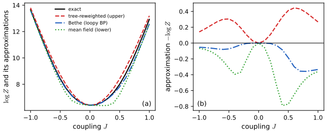
10.5 Tighter bounds
p. 473 Instead of enlarging the family, tighten the bound that \(q\) is fitted to.
10.5.1 Multi-sample ELBO (IWAE bound)
p. 473 With importance weights \(w_s=p_{\bm\theta}(\bm x,\bm z_s)/q_{\bm\phi}(\bm z_s\given\bm x)\), \(\bm z_s\sim q_{\bm\phi}\) independently, the average \(\hat p_S=\frac1S\sum_sw_s\) (10.166) is an unbiased estimate of \(p_{\bm\theta}(\bm x)\), and Jensen's inequality gives the IWAE bound (Burda, Grosse and Salakhutdinov, 2016) \[ \ELBO_S(\bm\phi,\bm\theta\given\bm x)=\E_{q(\bm z_{1:S})}\Big[\log\frac1S\sum_{s=1}^Sw_s\Big]\le\log p_{\bm\theta}(\bm x), \tag{10.167–10.168} \] with \(\ELBO_1\) the usual ELBO (10.169) and \(\ELBO_S\) non-decreasing in \(S\). (In (10.166)–(10.167) the book sums over \(k\) but indexes \(\bm z_s\), and writes \(w_s\) for what it has just defined as the normalised weights, whose average is always \(1/S\); the unnormalised weights \(w^*_s\) are meant.)
Filling the gap 10.25: unbiasedness, monotonicity in \(S\), and convergence of the IWAE bound p. 473, (10.166)–(10.169); [BGS16]
Proof
Unbiased. \(\E_q[w]=\int q\frac{p(\bm x,\bm z)}{q}\d\bm z=\int_{\{q>0\}}p(\bm x,\bm z)\d\bm z=p(\bm x)\) if \(q>0\) wherever \(p(\bm x,\cdot)>0\); then \(\E\hat p_S=p(\bm x)\), and Jensen (concavity of log) gives (10.168).
Monotone. Fix \(m<S\) and let \(I\) be a uniformly random \(m\)-subset of \(\{1,\dots,S\}\), independent of the draws. Each index lies in \(I\) with probability \(m/S\), so \(\E_I\big[\frac1m\sum_{i\in I}w_i\big]=\frac1S\sum_sw_s\). By Jensen, \(\log\frac1S\sum_sw_s\ge\E_I\log\frac1m\sum_{i\in I}w_i\). Take \(\E_q\): since the \(w_s\) are i.i.d., every subset average has the law of an \(m\)-sample average, so \(\ELBO_S\ge\ELBO_m\).
Convergence. Assume \(\E_q|\log w|<\infty\). By the strong law \(\hat p_S\to p(\bm x)\) almost surely, so \(\log\hat p_S\to\log p(\bm x)\). For uniform integrability: \(\log\hat p_S\le\hat p_S\), and averages of i.i.d. integrable variables are uniformly integrable; \(\log\hat p_S\ge\frac1S\sum_s\log w_s\) (Jensen), whose negative part is uniformly integrable for the same reason. By Vitali's theorem \(\ELBO_S\to\log p(\bm x)\). The gap behaves like \(\var(w)/(2Sp(\bm x)^2)\) when \(w\) has a finite variance (a second-order expansion of the log), so it can be very slow when \(q\) misses part of the posterior.
Example. For the toy model of Figure 10.x2, whose posterior has two symmetric modes, the ELBO-optimal Gaussian sits on one mode. Its draws practically never reach the other mode, so \(\hat p_S\) estimates the mass of one mode, \(\approx p(\bm x)/2\): the IWAE bound climbs quickly to \(\log p(\bm x)-\log2\) and stalls there (at \(S=500\), \(-2.735\) against \(\log p(\bm x)-\log2=-2.745\) and \(\log p(\bm x)=-2.052\)), even though it converges to \(\log p(\bm x)\) eventually. The broad moment-matched Gaussian has a terrible ELBO (\(-5.83\)) but reaches \(-2.053\) at \(S=500\). \(\square\)
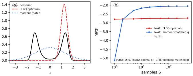
10.5.1.1 Pathologies of optimizing the IWAE bound
p. 474 As \(S\) grows the bound depends less on \(q\), and the signal-to-noise ratio of the \(\bm\phi\) gradient falls (like \(1/\sqrt S\); Rainforth et al., 2018). Remedies: the doubly reparameterised estimator, the TVO, reweighted wake-sleep.
10.5.2 The thermodynamic variational objective (TVO)
p. 474 The TVO (Masrani, Le and Wood, 2019) uses thermodynamic integration (path sampling) between \(q\) and the posterior.
Filling the gap 10.26: thermodynamic integration, and the ELBO and EUBO as its two crudest Riemann sums p. 474
Proof
For \(\beta\in[0,1]\) let \(\pi_\beta(\bm z)\propto q(\bm z)^{1-\beta}p(\bm x,\bm z)^\beta=q(\bm z)w(\bm z)^\beta\), with normaliser \(Z_\beta=\E_q[w^\beta]\); \(Z_0=1\), \(Z_1=p(\bm x)\). Differentiating under the integral (valid when \(\E_q[w^\beta|\log w|]<\infty\)): \(\frac{\d}{\d\beta}\log Z_\beta=\E_{\pi_\beta}[\log w]\), and once more \(\frac{\d^2}{\d\beta^2}\log Z_\beta=\var_{\pi_\beta}(\log w)\ge0\). Hence \[ \log p(\bm x)=\int_0^1\E_{\pi_\beta}[\log w]\,\d\beta, \] with a non-decreasing integrand. A left Riemann sum over \(0=\beta_0<\dots<\beta_K=1\) is therefore a lower bound, the TVO: \(\sum_k(\beta_k-\beta_{k-1})\E_{\pi_{\beta_{k-1}}}[\log w]\le\log p(\bm x)\). With one interval it is \(\E_q[\log w]=\) the ELBO; adding points can only raise it. A right Riemann sum is an upper bound, and with one interval it is \(\E_{p(\bm z|\bm x)}[\log w]=\log p(\bm x)+\Dkl(p(\cdot\given\bm x)\|q)\), the EUBO of Section 10.5.3. The expectations under \(\pi_\beta\) are estimated by self-normalised importance sampling from \(q\), which needs no reparameterisation, hence the method's appeal for discrete latents. \(\square\)
10.5.3 Minimizing the evidence upper bound
pp. 474–475 \(\mathrm{EUBO}(\bm\theta,\bm\phi\given\bm x)=\log p_{\bm\theta}(\bm x)+\Dkl\big(p_{\bm\theta}(\bm z\given\bm x)\|q_{\bm\phi}(\bm z\given\bm x)\big)\ge\log p_{\bm\theta}(\bm x)\) (10.171). Minimising it in \(\bm\phi\) is forward-KL (mass-covering) fitting; averaged over \(p_{\bm\theta}(\bm x)\) it is the sleep phase of Section 10.6.2, and over \(p_{\mathcal D}(\bm x)\) with self-normalised importance sampling it is the daydream phase. Its gradient is \[ \nabla_{\bm\phi}\mathrm{EUBO}=-\E_{p(\bm z|\bm x)}\big[\nabla_{\bm\phi}\log q_{\bm\phi}(\bm z\given\bm x)\big]\approx-\sum_{s=1}^S\bar w_s\nabla_{\bm\phi}\log q_{\bm\phi}(\bm z_s\given\bm x), \] the negative of the book's (10.172).
Filling the gap 10.27: the EUBO gradient and its sign pp. 474–475, (10.171)–(10.172)
Proof
\(\mathrm{EUBO}=\log p(\bm x)+\E_{p(\bm z|\bm x)}[\log p(\bm z\given\bm x)]-\E_{p(\bm z|\bm x)}[\log q_{\bm\phi}(\bm z\given\bm x)]\); only the last term depends on \(\bm\phi\), and the measure \(p(\bm z\given\bm x)\) does not, so \(\nabla_{\bm\phi}\mathrm{EUBO}=-\E_{p(\bm z|\bm x)}[\nabla_{\bm\phi}\log q_{\bm\phi}]\). Self-normalised importance sampling with proposal \(q_{\bm\phi}\) estimates \(\E_{p(\bm z|\bm x)}[h]\) by \(\sum_s\bar w_sh(\bm z_s)\), \(\bar w_s=w_s/\sum_{s'}w_{s'}\) (consistent as \(S\to\infty\), biased for finite \(S\)). Gradient descent on the EUBO therefore moves along \(+\sum_s\bar w_s\nabla\log q(\bm z_s)\), the daydream update; (10.172) as printed has the sign of the update, not of the gradient. Numerically, for \(q=\N(0.3,1)\) on the toy posterior, the finite-difference derivative of the EUBO in the mean of \(q\) equals \(-\E_p[\partial_m\log q]\) to \(10^{-6}\). \(\square\)
10.6 Wake-sleep algorithm
p. 475 Wake-sleep (Hinton et al., 1995; reweighted: Bornschein and Bengio, 2015; Le et al., 2019) trains the generative model and the inference network with two different objectives, avoiding REINFORCE for discrete latents.
10.6.1 Wake phase
pp. 475–476 Fit \(\bm\theta\) by maximum likelihood (10.173)–(10.174), with \(\log p_{\bm\theta}(\bm x)\) replaced by the IWAE estimate \(\log\frac1S\sum_sw_s\) (10.175). Its gradient is \(\sum_s\bar w_s\nabla\log w_s\) (10.176)–(10.179), and for \(\bm\theta\), \(\nabla_{\bm\theta}\log w_s=\nabla_{\bm\theta}\log p_{\bm\theta}(\bm x,\bm z_s)\) (10.180), so \[ \nabla_{\bm\theta}\ell(\bm\theta\given\bm\phi,\bm x)=\sum_{s=1}^S\bar w_s\nabla_{\bm\theta}\log p_{\bm\theta}(\bm x,\bm z_s). \tag{10.181} \]
10.6.2 Sleep phase
pp. 476–477 Fit \(\bm\phi\) by minimising \(\E_{p_{\bm\theta}(\bm x)}\Dkl(p_{\bm\theta}(\bm z\given\bm x)\|q_{\bm\phi}(\bm z\given\bm x))\) (10.182), i.e. maximum likelihood for \(q_{\bm\phi}\) on "dreamed" pairs \((\bm z'_s,\bm x'_s)\sim p_{\bm\theta}\) (10.183)–(10.185); the samples do not depend on \(\bm\phi\), so no reparameterisation is needed.
10.6.3 Daydream phase
p. 477 Use real data instead: minimise \(\E_{p_{\mathcal D}(\bm x)}\Dkl(p_{\bm\theta}(\bm z\given\bm x)\|q_{\bm\phi}(\bm z\given\bm x))\) (10.186), with gradient \(\approx\sum_s\bar w_s\nabla_{\bm\phi}\log q_{\bm\phi}(\bm z_s\given\bm x)\) for \(\bm z_s\sim q_{\bm\phi}\) (10.188).
10.6.4 Summary of algorithm
Algorithm 10.5: one SGD update of reweighted wake-sleep
- Sample \(\bm x_n\) from the data; draw \(\bm z_s\sim q(\bm z\given\bm x_n)\), \(s=1{:}S\); compute \(w_s=p(\bm x_n,\bm z_s)/q(\bm z_s\given\bm x_n)\) and \(\bar w_s=w_s/\sum_{s'}w_{s'}\); optionally \(\log p(\bm x_n)\approx\log\frac1S\sum_sw_s\).
- Wake: update \(\bm\theta\) along \(\sum_s\bar w_s\nabla_{\bm\theta}\log p_{\bm\theta}(\bm z_s,\bm x_n)\).
- Daydream: update \(\bm\phi\) along \(\sum_s\bar w_s\nabla_{\bm\phi}\log q_{\bm\phi}(\bm z_s\given\bm x_n)\).
- Optional sleep: draw \((\bm x'_s,\bm z'_s)\sim p_{\bm\theta}\) and update \(\bm\phi\) along \(\frac1S\sum_s\nabla_{\bm\phi}\log q_{\bm\phi}(\bm z'_s\given\bm x'_s)\).
pp. 477–478 RWS has no single objective, but its phases are two KL minimisations between \(p_{\bm\theta}(\bm x,\bm z)\) and \(q_{\mathcal D,\bm\phi}(\bm x,\bm z)=p_{\mathcal D}(\bm x)q_{\bm\phi}(\bm z\given\bm x)\) (10.189)–(10.190).
Filling the gap 10.28: the wake gradient, the sleep identity, and which KL each phase minimises pp. 475–478, (10.173)–(10.190)
Proof
(10.176)–(10.181). \(\nabla\log\frac1S\sum_sw_s=\frac{\sum_s\nabla w_s}{\sum_sw_s}=\frac{\sum_sw_s\nabla\log w_s}{\sum_{s'}w_{s'}}=\sum_s\bar w_s\nabla\log w_s\), using \(\nabla w=w\nabla\log w\) for \(w>0\). For fixed draws \(\bm z_s\), \(\log w_s=\log p_{\bm\theta}(\bm x,\bm z_s)-\log q_{\bm\phi}(\bm z_s\given\bm x)\) and the second term does not involve \(\bm\theta\): (10.180)–(10.181). (Confirmed by finite differences to \(10^{-6}\) on the toy model with \(\bm\theta=\sigma_x\).) For \(\bm\phi\) the draws themselves depend on \(\bm\phi\), so this is not the full \(\bm\phi\) gradient; RWS does not use it for \(\bm\phi\).
(10.182). \(\E_{p(\bm x)}\Dkl(p(\bm z\given\bm x)\|q(\bm z\given\bm x))=\E_{p(\bm x,\bm z)}[\log p(\bm z\given\bm x)]-\E_{p(\bm x,\bm z)}[\log q_{\bm\phi}(\bm z\given\bm x)]\); the first term does not depend on \(\bm\phi\).
(10.189), the wake phase. For a discrete empirical distribution, \(\Dkl(q_{\mathcal D,\bm\phi}\|p_{\bm\theta})=\E_{p_{\mathcal D}}\E_{q_{\bm\phi}}[\log p_{\mathcal D}(\bm x)+\log q_{\bm\phi}(\bm z\given\bm x)-\log p_{\bm\theta}(\bm x,\bm z)]=-\Hent(p_{\mathcal D})-\E_{p_{\mathcal D}}[\ELBO(\bm\theta,\bm\phi\given\bm x)]\): minimising it in \(\bm\theta\) is ELBO maximisation (the original wake phase; RWS uses the IWAE surrogate instead).
(10.190). As a function of \(\bm\phi\), \(\Dkl(p_{\bm\theta}\|q_{\mathcal D,\bm\phi})=-\E_{p_{\bm\theta}(\bm x,\bm z)}[\log q_{\bm\phi}(\bm z\given\bm x)]\)+const, which is the sleep objective (10.183), not the daydream objective (10.186) as labelled (and it is formally infinite unless \(p_{\bm\theta}(\bm x)\) lives on the data points). The daydream objective is \(\E_{p_{\mathcal D}}\Dkl(p_{\bm\theta}(\bm z\given\bm x)\|q_{\bm\phi}(\bm z\given\bm x))=\Dkl\big(p_{\mathcal D}(\bm x)p_{\bm\theta}(\bm z\given\bm x)\,\|\,p_{\mathcal D}(\bm x)q_{\bm\phi}(\bm z\given\bm x)\big)\), a KL between two joints that share the data marginal. \(\square\)
10.7 Expectation propagation (EP)
p. 478 Standard VI minimises \(\Dkl(q\|p)\), which is zero forcing and tends to be over-confident; EP (Minka, 2001) is a local approximation to the mass-covering \(\Dkl(p\|q)\).
See also: Bishop course, Section 10.7 (EP and the clutter problem), its EP demo.
10.7.1 Algorithm
pp. 478–480 Write the posterior as \(p(\bm\theta\given\mathcal D)\propto p_0(\bm\theta)\prod_{k=1}^Kf_k(\bm\theta)\) (10.191) and the approximation as \(q\propto p_0\prod_k\tilde f_k\) with \(\tilde f_k\) in an exponential family \(\mathcal Q\) (10.192). For each \(i\) in turn: form the cavity \(q_{-i}\propto q/\tilde f_i\) (10.193; subtract natural parameters), the tilted distribution \(q_i^{\rm tilted}=f_iq_{-i}/Z_i\) (10.194), its projection \(\argmin_{\tilde q\in\mathcal Q}\Dkl(q_i^{\rm tilted}\|\tilde q)\) (10.195; moment matching), and the new site \(\tilde f_i^{\rm new}=q_i^{\rm proj}/q_{-i}\) (10.198). Replacing moment matching by a Laplace approximation of the tilted distribution, (10.196)–(10.197), is Laplace propagation (the \(\alpha\) in (10.196) belongs to power EP, Section 10.7.5, and should be 1 here).
Filling the gap 10.29: the projection is moment matching, the site update in natural parameters, and what an EP fixed point is pp. 478–480, (10.191)–(10.198)
Proof
Projection. For \(\mathcal Q\) an exponential family with statistics \(\bm T\), \(\Dkl(r\|q_{\bm\eta})\) is convex in \(\bm\eta\) with gradient \(\E_{q_{\bm\eta}}\bm T-\E_r\bm T\), so the minimiser matches moments (gap 5.4). For Gaussians: the mean and covariance of the tilted distribution.
Natural parameters. If \(q\) and the sites are unnormalised exponential-family terms, \(q\propto\exp(\bm\lambda^\T\bm T)\) with \(\bm\lambda=\bm\lambda_0+\sum_k\tilde{\bm\lambda}_k\). Division is subtraction, \(\bm\lambda_{-i}=\bm\lambda-\tilde{\bm\lambda}_i\), and the new site is \(\tilde{\bm\lambda}_i^{\rm new}=\bm\lambda^{\rm proj}-\bm\lambda_{-i}\). Sites need not be normalisable (a site's "precision" can be negative); only the cavity must be (otherwise the tilted moments do not exist), which is the numerical fragility of Section 10.7.4.
Fixed points. At convergence \(\tilde f_i^{\rm new}=\tilde f_i\) for every \(i\), i.e. \(q_{-i}\tilde f_i=q\) equals the projection of \(f_iq_{-i}\): \(q\) has the same moments \(\E\bm T\) as every tilted distribution simultaneously. This characterisation does not mention the update order, which is why EP, unlike ADF, gives an order-independent answer at convergence. If every \(f_i\) is itself in \(\mathcal Q\), the tilted distributions are already in \(\mathcal Q\), the first sweep is exact and \(q\) is the posterior. Otherwise EP is not guaranteed to converge and its fixed point is not the global moment projection of \(p\): on the 12-point logistic example below, the EP fixed point (verified: all 12 tilted distributions have \(q\)'s mean and variance to \(10^{-8}\)) has variance 0.311, the exact posterior 0.389. \(\square\)
10.7.2 Example
p. 480 Multiplying a very non-Gaussian logistic factor into a Gaussian cavity gives a nearly Gaussian tilted distribution, so the projection loses little: EP Gaussianises each factor in the context of all the others, not in isolation.
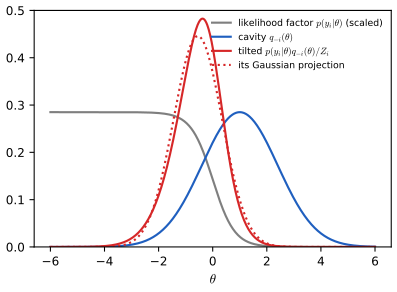
10.7.3 EP as generalized ADF
pp. 480–481 Assumed density filtering processes each factor once, projecting \(q_t\propto q_{t-1}f_t\) back to \(\mathcal Q\); the result depends on the order, and re-passing the data multiplies the same factor in again (over-confidence). EP keeps each factor's contribution as a site and replaces it rather than adding to it.
10.7.4 Optimization issues
p. 481 Damping replaces the site by \(\tilde f_i^{1-\delta}(q_i^{\rm proj}/q_{-i})^\delta\) (10.199), i.e. a convex combination of site natural parameters; \(\delta=1/K\) is safe but slow, starting at 0.5 and decreasing is a common schedule. EP need not converge, but usually does for log-concave factors.
10.7.5 Power EP and α-divergence
p. 481 Power EP (Minka, 2004) uses the cavity \(q/\tilde f_i^\alpha\), projects \(q_{-i}f_i^\alpha\) and sets \(\tilde f_i^{\rm new}\propto(q^{\rm proj}_i/q_{-i})^{1/\alpha}\); \(\alpha=1\) is EP and \(\alpha\to0\) approaches the reverse KL of VI.
Filling the gap 10.30: ADF's order dependence, damping keeps the fixed points, and power EP between EP and VI pp. 480–481, (10.199)
Proof
ADF. The projection does not commute with multiplying in further factors (the moments of \(\operatorname{proj}(q f_1)f_2\) differ from those of \(qf_1f_2\) unless the factors are in \(\mathcal Q\)), so the final \(q\) depends on the order. On the logistic example ADF gives \(\N(1.47,0.33)\) in the given order and \(\N(1.02,0.87)\) in reverse order; EP gives the same fixed point \(\N(1.111,0.311)\) for both orders.
Damping. In natural parameters (10.199) is \(\tilde{\bm\lambda}_i\leftarrow(1-\delta)\tilde{\bm\lambda}_i+\delta\tilde{\bm\lambda}_i^{\rm new}\); a fixed point of the damped map has \(\tilde{\bm\lambda}_i=\tilde{\bm\lambda}_i^{\rm new}\), the undamped fixed-point condition. Damping changes the path, not the answer (with \(\delta=0.3\) and 200 sweeps the example reaches the same fixed point to \(10^{-7}\)).
Power EP. The local step minimises an \(\alpha\)-divergence between \(q_{-i}f_i\) and \(q_{-i}\tilde f_i\) instead of the KL (Minka, 2004); the \(\alpha\)-divergences interpolate between \(\Dkl(p\|q)\) at \(\alpha=1\) and \(\Dkl(q\|p)\) as \(\alpha\to0\) (gap 2.26). The iteration's fixed points are the stationary points of the corresponding local objective; for small \(\alpha\) they approach the stationary points of the VI objective. On the example: EP variance 0.311, power EP with \(\alpha=0.05\) 0.2987, VI 0.2981, exact 0.389. Here even EP is well below the exact variance, because the posterior is skewed (skewness 0.85; the Gaussian family cannot carry the long right tail through the local projections). \(\square\)
10.7.6 Stochastic EP
pp. 481–482 EP stores one site per data point (\(O(ND^2)\) memory for full Gaussians). Stochastic EP (Li, Hernández-Lobato and Turner, 2015) keeps one shared site \(\tilde f\) with \(\prod_nf_n\approx\tilde f^N\) (10.200): cavity \(q/\tilde f\) (10.201), tilted \(f_nq_{-1}\) (10.202), local site by moment matching (10.203), and the damped update \(\tilde f\leftarrow\tilde f^{1-1/N}\tilde f_n^{1/N}\) (10.204), a running average of the local sites' natural parameters. ADF instead uses the previous posterior as the cavity, which in the batch setting counts data repeatedly.
Practice problems
The book has no end-of-chapter exercises for Chapter 10, so here are three short problems of my own, with complete solutions (hidden).
Practice problem 10.1 (CAVI on a correlated Gaussian). The target is \(p(\bm z)=\N(\bm\mu,\bm\Sigma)\) in two dimensions with unit variances and correlation \(r\); \(q=q_1(z_1)q_2(z_2)\). (a) Derive the CAVI updates. (b) Show that the error in the means shrinks by \(r^2\) per sweep and find the number of sweeps needed to reduce it by \(10^6\) when \(r=0.9\). (c) What are the final variances and the final KL?
Solution
(a) With \(\bm\Lambda=\bm\Sigma^{-1}\), \(\log p=-\frac12\Lambda_{11}(z_1-\mu_1)^2-\Lambda_{12}(z_1-\mu_1)(z_2-\mu_2)+\cdots\). By (10.87), \(\log q_1(z_1)=-\frac12\Lambda_{11}z_1^2+z_1[\Lambda_{11}\mu_1-\Lambda_{12}(m_2-\mu_2)]\)+const, so \(q_1=\N(m_1,1/\Lambda_{11})\) with \(m_1=\mu_1-\frac{\Lambda_{12}}{\Lambda_{11}}(m_2-\mu_2)\), and symmetrically for \(q_2\). (b) With errors \(e_j=m_j-\mu_j\): \(e_1\leftarrow-\frac{\Lambda_{12}}{\Lambda_{11}}e_2\), then \(e_2\leftarrow-\frac{\Lambda_{12}}{\Lambda_{22}}e_1\), so one sweep multiplies \(e_2\) by \(\frac{\Lambda_{12}^2}{\Lambda_{11}\Lambda_{22}}=r^2\) (for unit variances \(\bm\Lambda=\frac1{1-r^2}\left(\begin{smallmatrix}1&-r\\-r&1\end{smallmatrix}\right)\)). For \(r=0.9\): \(0.81^n\le10^{-6}\) needs \(n\ge\ln10^{-6}/\ln0.81=65.6\), so 66 sweeps: strongly correlated targets make CAVI slow. (c) Variances \(1/\Lambda_{jj}=1-r^2=0.19\), and \(\Dkl(q\|p)=-\frac12\log(1-r^2)=0.830\) nats (gap 5.5), the ELBO gap at convergence. \(\square\)
Practice problem 10.2 (two spins). \(p(z_1,z_2)\propto\exp(Jz_1z_2)\), \(z_i\in\{\pm1\}\), \(J=2\). (a) Compute \(\log Z\). (b) Find all mean-field fixed points \(\mu_1=\mu_2=\mu\) and their ELBOs. (c) What does the Bethe approximation give, and why?
Solution
(a) \(Z=2e^J+2e^{-J}=4\cosh J\), \(\log Z=\log(4\cosh2)=2.7113\). (b) The ELBO is \(J\mu_1\mu_2+\Hent_b(\frac{1+\mu_1}2)+\Hent_b(\frac{1+\mu_2}2)\) and the update \(\mu_1=\tanh(J\mu_2)\) (gap 10.12). Symmetric fixed points solve \(\mu=\tanh(2\mu)\): \(\mu=0\) (ELBO \(2\log2=1.3863\)) and \(\mu=\pm0.9575\) (ELBO 2.0393). Since \(\tanh\) has slope \(J\) at 0, non-zero solutions exist iff \(J>1\), and then \(\mu=0\) is a saddle: mean field "breaks the symmetry" and picks one of the two aligned states, losing about \(\log2\) (2.7113 \(-\) 2.0393 = 0.672). (c) A single edge is a tree, so the Bethe entropy is exact and BP returns \(\log Z=2.7113\) and the exact marginals \(\Pr(z_i=1)=\frac12\) (gap 10.23). \(\square\)
Practice problem 10.3 (why constants hurt the score-function gradient). Let \(q=\N(\mu,1)\) and \(\log\tilde p(z)=-\frac12(z-a)^2+C\) (an unnormalised Gaussian target). For the score-function estimate of \(\partial\ELBO/\partial\mu\) with one sample, (a) compute its mean and variance; (b) find the optimal control-variate constant and the resulting variance; (c) evaluate for \(a-\mu=1\), \(C=10\).
Solution
With \(\epsilon=z-\mu\sim\N(0,1)\) and \(d=a-\mu\): \(\tilde L=\log\tilde p(z)-\log q(z)=-\frac12(\epsilon-d)^2+\frac12\epsilon^2+C+\frac12\log2\pi=d\epsilon+k\), where \(k=C+\frac12\log2\pi-\frac12d^2\). The score is \(g=\epsilon\). (a) The estimate is \(g\tilde L=d\epsilon^2+k\epsilon\): mean \(d\) (the true gradient), variance \(d^2\var(\epsilon^2)+k^2\var(\epsilon)+2dk\cov(\epsilon^2,\epsilon)=2d^2+k^2\). (b) \(c^*=\E[g^2\tilde L]/\E[g^2]=\E[d\epsilon^3+k\epsilon^2]=k\) (gap 10.9), and \(g(\tilde L-k)=d\epsilon^2\) has variance \(2d^2\): the control variate removes exactly the constant, which carries no information, and at the optimum \(d=0\) the estimate has zero variance. (c) \(k=10+0.919-0.5=10.42\): variance \(2+108.6=110.6\) without, 2 with the control variate. \(\square\)
Demonstrations
- Mean-field Ising denoising (Section 10.3.2): coupling, noise, damping, parallel against sequential updates, the ELBO sweep by sweep.
- The ELBO, the IWAE bound and the EUBO (Sections 10.1, 10.5): a Gaussian \(q\) on a bimodal posterior, the three bounds against \(\log p(x)\).
- Expectation propagation for a logistic model (Section 10.7): cavity, tilted and projected distributions site by site; EP, ADF, damping, power EP, VI and the exact posterior.
Python code for every figure: code index. Data used by the demos: data/ch10-ising.json, data/ch10-bounds.json, data/ch10-ep.json. Companion demos: VB for a Gaussian, the variational mixture of Gaussians, EP for the clutter problem.
Notes on the book
Points where the book is imprecise or wrong
- (10.49). The alternative objective should be \(\log p(\bm x\given\bm z)-\Dkl(q\|p)\), not \(+\) (gap 10.5).
- (10.50). The Gaussian KL misses \(-\frac12\) per coordinate; as printed it equals \(K/2\) at \(q=p\) (gap 10.5).
- (10.37). The covariance of \(\bm\mu+\bm\epsilon\odot\bm\sigma\) is \(\diag(\bm\sigma^2)\), not \(\diag(\bm\sigma)\).
- Section 10.3.6.4. "The digamma function, which is always positive": \(\dg(x)<0\) for \(x<1.46\); it is \(e^{\dg}\) that is positive (gap 10.15).
- (10.150)–(10.151). \(\tilde\Lambda_k\) is defined as the expected quadratic form and then used as \(e^{\E\log|\bm\Lambda_k|}\); (10.151) writes \(\hat{\bm\Lambda}_k\) for \(\hat{\bm L}_k\).
- (10.165). The bracket should be \(\nabla_{\bm z}[\log p(\bm x,\bm z)-\log p(\bm x)]\).
- (10.166)–(10.167). The sums run over \(k\) but index \(\bm z_s\), and \(w_s\) (defined as normalised weights) is used where the unnormalised \(w^*_s\) is meant.
- (10.172). \(\nabla_{\bm\phi}\mathrm{EUBO}=-\sum_s\bar w_s\nabla\log q\); the printed sign is that of the descent direction (gap 10.27).
- (10.190). As a function of \(\bm\phi\), \(\Dkl(p_{\bm\theta}\|q_{\mathcal D,\bm\phi})\) is the sleep objective, not the daydream one (gap 10.28).
- (10.196). The factor \(\alpha\) belongs to power EP (Section 10.7.5); in plain EP it is 1. Algorithm 10.5 also has a stray "b" as line 9.
- Figure 10.10. The caption's colours (orange and blue) disagree with the text (green and red).
- Supplement S(10.17). The Gauss–Newton step needs a minus sign, as in S(10.10) (gap 10.7).
- Supplement S(10.22). The quantity called \(\ELBO_t\) is the negative ELBO \(-\ELBO_t\) of S(10.19) (gap 10.10).
- Supplement S(10.38), S(10.44), S(10.46). \(q\) has natural parameter \(\bm\lambda\), not \(\bm\eta\); the two mirror-descent problems are maximisations (argmax), not argmin (gap 10.18).
- Supplement 10.4. "\(Z=\log p(\bm x)\), \(\tilde p(\bm z)=\bm T(\bm z)^\T\bm\theta\)" should be \(Z=p(\bm x)\), \(\log\tilde p(\bm z)=\bm T(\bm z)^\T\bm\theta\).
- Supplement 10.4.3.1. For attractive models the Bethe value is a lower bound on \(\log Z\) (Sudderth, Wainwright and Willsky, 2008; Ruozzi, 2012), not an upper bound; confirmed on a 3×3 grid (gap 10.23, Figure 10.x3). After S(10.93), positivity of \(\bm\tau\) at the optimum comes from the entropy, not from \(\bm\theta>0\).
References
- Murphy, K. P. (2023). Probabilistic Machine Learning: Advanced Topics. MIT Press, Cambridge, MA. Chapter 10, pp. 439–482, and supplementary material, Chapter 10. probml.github.io/pml-book/book2.html.
- Bishop, C. M. (2006). Pattern Recognition and Machine Learning. Springer, New York. Chapter 10.
- Blei, D. M., Kucukelbir, A. and McAuliffe, J. D. (2017). Variational inference: a review for statisticians. Journal of the American Statistical Association, 112(518), 859–877.
- Bornschein, J. and Bengio, Y. (2015). Reweighted wake-sleep. International Conference on Learning Representations.
- Burda, Y., Grosse, R. and Salakhutdinov, R. (2016). Importance weighted autoencoders. International Conference on Learning Representations.
- Ghahramani, Z. and Jordan, M. I. (1997). Factorial hidden Markov models. Machine Learning, 29, 245–273.
- Hoffman, M. D., Blei, D. M., Wang, C. and Paisley, J. (2013). Stochastic variational inference. Journal of Machine Learning Research, 14, 1303–1347.
- Khan, M. E. and Lin, W. (2017). Conjugate-computation variational inference. Proceedings of AISTATS.
- Kucukelbir, A., Tran, D., Ranganath, R., Gelman, A. and Blei, D. M. (2017). Automatic differentiation variational inference. Journal of Machine Learning Research, 18(14), 1–45.
- Le, T. A., Kosiorek, A. R., Siddharth, N., Teh, Y. W. and Wood, F. (2019). Revisiting reweighted wake-sleep for models with stochastic control flow. Uncertainty in Artificial Intelligence.
- Li, Y., Hernández-Lobato, J. M. and Turner, R. E. (2015). Stochastic expectation propagation. Advances in Neural Information Processing Systems, 28.
- Masrani, V., Le, T. A. and Wood, F. (2019). The thermodynamic variational objective. Advances in Neural Information Processing Systems, 32.
- Minka, T. P. (2001). Expectation propagation for approximate Bayesian inference. Uncertainty in Artificial Intelligence. Minka, T. P. (2004). Power EP. Technical report, Microsoft Research.
- Rainforth, T., Kosiorek, A. R., Le, T. A., Maddison, C. J., Igl, M., Wood, F. and Teh, Y. W. (2018). Tighter variational bounds are not necessarily better. International Conference on Machine Learning.
- Ranganath, R., Gerrish, S. and Blei, D. M. (2014). Black box variational inference. Proceedings of AISTATS. Ranganath, R., Tran, D. and Blei, D. M. (2016). Hierarchical variational models. International Conference on Machine Learning.
- Ruozzi, N. (2012). The Bethe partition function of log-supermodular graphical models. Advances in Neural Information Processing Systems, 25.
- Sudderth, E. B., Wainwright, M. J. and Willsky, A. S. (2008). Loop series and Bethe variational bounds in attractive graphical models. Advances in Neural Information Processing Systems, 20.
- Wainwright, M. J. and Jordan, M. I. (2008). Graphical models, exponential families, and variational inference. Foundations and Trends in Machine Learning, 1(1–2), 1–305.
- Winn, J. and Bishop, C. M. (2005). Variational message passing. Journal of Machine Learning Research, 6, 661–694.
- Yedidia, J. S., Freeman, W. T. and Weiss, Y. (2005). Constructing free-energy approximations and generalized belief propagation algorithms. IEEE Transactions on Information Theory, 51(7), 2282–2312.
- Zeno, C., Golan, I., Hoffer, E. and Soudry, D. (2021). Task-agnostic continual learning using online variational Bayes with fixed-point updates. Neural Computation, 33(11), 3139–3177.
The numerical statements in the text (the ELBO identities, the reparameterised densities and the Gaussian KL, the low-rank algebra, the sparsity of the optimal Gaussian precision, the ADVI fits, the score-function variances, the Ising, univariate-Gaussian and mixture VB results, the digamma inequalities, the IWAE, EUBO and wake-sleep identities, the EP fixed points, the FOO-VB and CVI results, and the mean-field, Bethe and tree-reweighted bounds) were confirmed numerically.