State-space models
A state-space model has a hidden state that evolves in time and observations emitted from it. This chapter is a catalogue of the models and of how to learn them: hidden Markov models (discrete states) fitted by EM, gradient descent, spectral methods or Gibbs sampling, with explicit durations and run-length changepoint detection; linear dynamical systems for tracking, recursive least squares and forecasting, with EM and subspace identification; switching, nonlinear and non-Gaussian relatives; structural time series for trend, season, forecasting and causal impact; and deep state-space models with their variational bounds. These notes prove what the book states, correct the slips, and show on simulated and public data what each model does.
Ch. 1 Introduction Ch. 2 Probability Ch. 3 Statistics Ch. 4 Graphical models Ch. 5 Information theory Ch. 6 Optimisation Ch. 7 Inference algorithms Ch. 8 Gaussian filtering Ch. 9 Message passing Ch. 10 Variational inference Ch. 11 Monte Carlo Ch. 12 MCMC Ch. 13 Sequential Monte Carlo Ch. 14 Predictive models Ch. 15 GLMs Ch. 16 Deep networks Ch. 17 Bayesian neural networks Ch. 18 Gaussian processes Ch. 19 Beyond iid Ch. 20 Generative models Ch. 21 VAEs Ch. 22 Autoregressive models Ch. 23 Normalizing flows Ch. 24 Energy-based models Ch. 25 Diffusion models Ch. 26 GANs Ch. 27 Discovery methods Ch. 28 Latent factor models Ch. 29 State-space models Ch. 30 Graph learning Ch. 31 Nonparametric Bayes Ch. 32 Representation learning Ch. 33 Interpretability Ch. 34 Decision making Ch. 35 Reinforcement learning Ch. 36 Causality
How to read these notes
They follow the book. Sections carry the book's numbers (29.4.1, 29.12.6, ...) and displayed equations that appear in the book carry its equation numbers, e.g. \((29.51)\). Material from the online supplement is placed where it belongs and labelled (supplement); its equations are cited as (S29.k).
Filling the gaps. Wherever the book states a result without proof, leaves a calculation to the reader or quotes the literature, an orange Filling the gap box gives the argument. Derivations start hidden: open one with its bar, or use the button below. Results already proved in full elsewhere on this site are stated and linked rather than repeated.
Figures and demonstrations. Every figure of the chapter that is computed from a model or a simulation is reproduced from scratch by the Python code. Not redrawn: the diagrams and schematics (Figures 29.1, 29.9–29.12, 29.16–29.21, 29.25, 29.27–29.29, 29.32, 29.38–29.40, 29.42–29.45, S29.1, S29.2, S29.6), the figures taken from papers or photographs (29.10, 29.37), Figure 29.23 (a repeat of Figure 8.2, see Chapter 8) and Figures 29.34–29.36 (the 2014 Victoria electricity data are not available; anomaly detection is shown in the extra Figure x29.a). Figures named x29.a are extra ones made for the notes. The ▶ Demo boxes open an interactive demonstration set to the case being discussed.
Main reference
K. P. Murphy, Probabilistic Machine Learning: Advanced Topics, MIT Press (2023; the December 2025 draft is followed), Chapter 29, pages 979–1042 of the printed numbering (PDF pages 1013–1076), and Supplementary Chapter 29, pages 219–226 (book web page: probml.github.io/pml-book/book2.html). Section, equation and figure numbers refer to this book. Chapter 29 has no end-of-chapter exercises, so three short practice problems with solutions are added at the end.
The explanations, derivations, figures and code are my own; equations are cited by their numbers in the book. Data: simulation throughout, and the monthly Mauna Loa CO2 record 1958–2001 shipped with statsmodels as a stand-in for the book's 1966–2019 record.
Companion courses
- The inference algorithms used throughout: forwards, forwards–backwards, Viterbi and forwards-filter backwards-sample for HMMs in Section 9.2; the Kalman filter, RTS smoother and the extended and unscented filters in Chapter 8 (also the Gaussian-sum approximation for switching models, Section 8.6.2); particle filters in Chapter 13; the EM algorithm in Section 6.5.3; matrix-normal inverse-Wishart regression in Section 15.2.9; the GP model of the same CO2 series in Section 18.8.1.
- HMMs and linear dynamical systems in Bishop's notation, with the EM derivations: Bayesian and Probabilistic ML, Section 13.2 (maximum likelihood for the HMM) and Section 13.3 (learning in LDS). Time series in the first volume: Murphy's first volume, Chapter 15.
New here: the AR-HMM steady state, the scaled likelihood trick, the HMM likelihood gradient as expected counts, the fixed point of identical states, the spectral (observable-operator) proof, the conjugate updates of the Gibbs samplers, the negative binomial duration, the exactness of BOCPD, the white-noise-acceleration covariance, the EM updates for LDS as a single regression lemma and the lag-one covariance, subspace identification, the exponential growth of the SLDS filter, the Laplace EM for the Poisson LDS, the local level as exponential smoothing, cubic forecast variance, the joint forecast covariance behind causal impact, the deep-SSM bounds, and the discretisation and convolution facts of the supplement.
29.1 Introduction
pp. 1013–1014, (29.1)–(29.7) A state-space model (SSM) is a partially observed Markov chain: a hidden state \(\vz_t\) evolves by a Markov transition, and each state emits an observation \(\vy_t\). The book writes it as a noisy dynamical system and as a probabilistic model,
\[ \vz_t=f(\vz_{t-1},\vu_t,\mathbf q_t),\quad \vy_t=h(\vz_t,\vu_t,\vy_{1:t-1},\mathbf r_t), \tag{29.1–29.2} \] \[ p(\vy_{1:T},\vz_{1:T}\given\vu_{1:T})=\Big[p(\vz_1\given\vu_1)\prod_{t=2}^{T}p(\vz_t\given\vz_{t-1},\vu_t)\Big]\Big[\prod_{t=1}^{T}p(\vy_t\given\vz_t,\vu_t,\vy_{1:t-1})\Big], \tag{29.5} \]where \(\vu_t\) are optional observed inputs. If the observation also depends on the previous observation the model is an autoregressive SSM (Figure 29.1a); a sufficiently rich state can carry that memory itself, so the usual choice is conditional independence of the observations given the states, which simplifies the product to
\[ p(\vy_{1:T},\vz_{1:T}\given\vu_{1:T})=\Big[p(\vz_1\given\vu_1)\prod_{t=2}^{T}p(\vz_t\given\vz_{t-1},\vu_t)\Big]\Big[\prod_{t=1}^{T}p(\vy_t\given\vz_t,\vu_t)\Big], \tag{29.6} \]and without inputs to (29.7). Inference for these models (the Bayes filter and smoother, which both questions of this chapter rely on) is treated in Chapter 8 and, for discrete states, in Section 9.2. This chapter is about the models: the hidden Markov model (discrete states), the linear dynamical system and its switching, nonlinear and structural-time-series relatives, and deep state-space models.
Chapter at a glance
- 29.2–29.5 HMMs: observation models, applications, learning by EM, by gradient descent, by spectral methods and by Gibbs sampling, and the extensions to explicit durations, hierarchies, several chains and changepoint detection (Filling the gap 29.3, 29.4, 29.5, 29.7, 29.8).
- 29.6–29.8 Linear dynamical systems: tracking, recursive least squares, EM and subspace identification (29.9–29.11).
- 29.9–29.11 Switching, nonlinear and non-Gaussian models (29.12–29.14).
- 29.12 Structural time series: local level, trend, season, forecasting and causal impact (29.15–29.17).
- 29.13 Deep SSMs and their variational bounds (29.18, 29.19). Supplement: continuous-time models and S4 (29.20, 29.21).
Notation. \(K\) hidden states, \(\mathbf A\) (written \(A_{jk}=p(z_t=k\given z_{t-1}=j)\)) the transition matrix, \(\bm\pi\) the initial distribution, \(\mathbf B\) categorical emissions \(B_{kv}=p(y_t=v\given z_t=k)\); \(N_z,N_y\) state and observation dimensions for linear models.
29.2 Hidden Markov models (HMMs)
p. 1014 A hidden Markov model is an SSM with discrete states \(z_t\in\{1,\dots,K\}\); the observations may be discrete, continuous or mixed. The notes of Chapter 9 prove the forwards, forwards–backwards and Viterbi algorithms; here they are used as black boxes (code: hmm_forward, hmm_estep, hmm_viterbi). Companion proofs in Bishop's notation: Bayesian and Probabilistic ML, Section 13.2.
29.2.1 Conditional independence properties
p. 1014, Figure 29.1b The graphical model of an HMM says two things: the states form a first-order Markov chain, and given the states the observations are independent. Everything else is the choice of the three ingredients below.
29.2.2 State transition model
pp. 1014–1015, (29.8)–(29.9) The initial distribution is \(p(z_1=j)=\pi_j\) and the transition matrix is row stochastic, \(p(z_t=j\given z_{t-1}=i)=A_{ij}\) with \(\sum_jA_{ij}=1\); its non-zero pattern is drawn as a state transition diagram.
29.2.3 Discrete likelihoods
p. 1015, (29.10)–(29.12) For categorical observations \(p(y_t=k\given z_t=j)=B_{jk}\) (the book calls the matrix \(y\), a clash with the observation, which we avoid). With \(D\) discrete observations per step the factorial forms (29.11) (categorical) and (29.12) (binary) multiply one factor per coordinate. The casino HMM of Section 9.2.1.1 is the standard example; Figure 29.2 samples from a five-state HMM with ten Bernoulli observables, and one sees the observation pattern switch each time the state does.
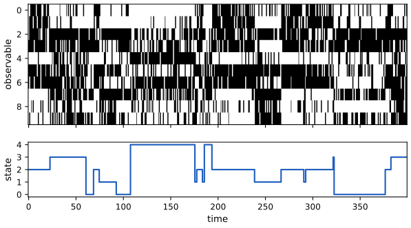
fig_29_2. Download: PDF · SVG29.2.4 Gaussian likelihoods
p. 1016, (29.13)–(29.14) For continuous data \(p(\vy_t\given z_t=j)=\N(\vy_t\given\bmu_j,\bSig_j)\) (29.13), or a Gaussian mixture per state (29.14), the GMM-HMM. A 2d example places the Gaussians as ellipses (the "lily pads"): the chain hops between pads, staying on one for a while. Compared with a plain Gaussian mixture the data are the same clusters but with temporal correlation.
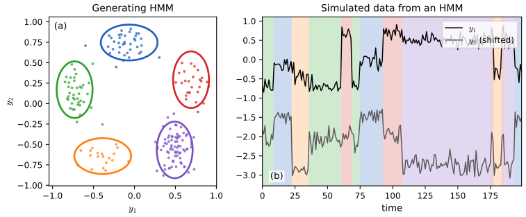
fig_29_3. Download: PDF · SVG29.2.5 Autoregressive likelihoods
pp. 1016–1018, (29.15)–(29.16) The conditional independence of observations is often false. Adding arcs \(\vy_{t-1}\to\vy_t\) gives the autoregressive HMM, with state-dependent regression
\[ p(\vy_t\given\vy_{t-1},z_t=j)=\N(\vy_t\given\mathbf E_j\vy_{t-1}+\bmu_j,\bSig_j), \tag{29.15} \](a regime-switching Markov model in econometrics) and, for lag \(L\), (29.16). Because every \(\vy\) is observed, the extra arcs change only the likelihood and not the difficulty of inference over \(z_{1:T}\).
Filling the gap 29.1: the steady state of an AR regime and when the dynamics converge to it p. 1017
The book says that if the chain stays in state \(j\) the observations converge to \(\vy^*_j=(\mI-\mathbf E_j)^{-1}\bmu_j\), and then sets \(\mathbf E_j\) to a rotation by 7 degrees. A pure rotation has eigenvalues of modulus 1, so there is no convergence; what is needed is spectral radius below 1.
Derivation
Fix the state and write \(\vy_t=\mathbf E\vy_{t-1}+\bmu+\bm\epsilon_t\) with \(\E\bm\epsilon_t=\mathbf0\). The mean \(\vm_t=\E\vy_t\) obeys \(\vm_t=\mathbf E\vm_{t-1}+\bmu\). A fixed point \(\vy^*\) satisfies \(\vy^*=\mathbf E\vy^*+\bmu\), i.e. \((\mI-\mathbf E)\vy^*=\bmu\), which has a unique solution exactly when 1 is not an eigenvalue of \(\mathbf E\). Subtracting, \(\vm_t-\vy^*=\mathbf E(\vm_{t-1}-\vy^*)\), hence \(\vm_t-\vy^*=\mathbf E^t(\vm_0-\vy^*)\). If the spectral radius \(\rho(\mathbf E)<1\) then \(\mathbf E^t\to\mathbf0\) geometrically at rate \(\rho(\mathbf E)^t\), so \(\vm_t\to\vy^*\). If the eigenvalues have modulus 1 (a rotation), \(\vm_t\) circles around \(\vy^*\) for ever, and the noisy process random-walks away. The covariance of a stable regime converges to the solution of the Lyapunov equation \(\bSig_\infty=\mathbf E\bSig_\infty\mathbf E^\T+\bSig_j\).
For \(\mathbf E=\rho\,\mathbf R(\theta)\) (a damped rotation), \((\mI-\mathbf E)^{-1}\) is a rotation scaled by \(1/|1-\rho e^{i\theta}|=(1-2\rho\cos\theta+\rho^2)^{-1/2}\); for \(\theta=7^\circ\), \(\rho=0.93\) this is 7.30. With \(\|\bmu_j\|=0.59\) the attractors are at distance 4.3 from the origin and, with the five \(\bmu_j\) spaced 72 degrees apart, the second and third are at \((-2.0,3.8)\) and \((-4.2,-0.8)\), the values quoted in the text. Figures 29.4 and 29.5 are drawn with this damped model. Confirmed numerically: the iteration reaches \(\vy^*\) to \(10^{-8}\). ∎
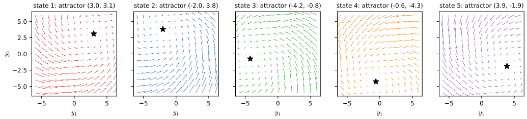
fig_29_4. Download: PDF · SVG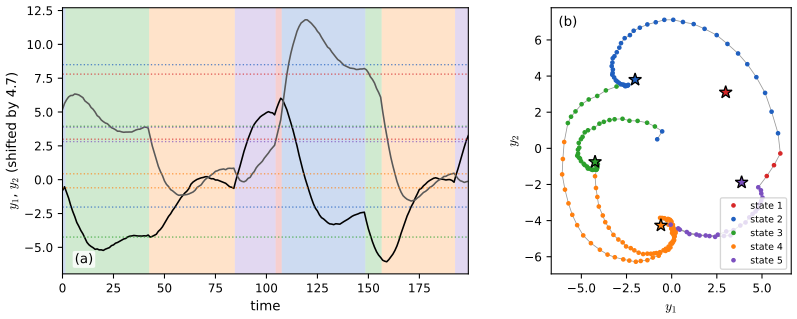
fig_29_5. Download: PDF · SVG29.2.6 Neural network likelihoods
pp. 1017–1018, (29.17) For images one can use a normalizing flow per state, or a classifier \(p(z_t=j\given\vy_t)\) turned into a likelihood by Bayes' rule, the scaled likelihood trick:
\[ p(\vy_t\given z_t=j)=\frac{p(z_t=j\given\vy_t)\,p(\vy_t)}{p(z_t=j)}\ \propto\ \frac{p(z_t=j\given\vy_t)}{p(z_t=j)}. \tag{29.17} \]Filling the gap 29.2: why dropping \(p(\vy_t)\) is harmless p. 1018, (29.17)
The factor \(p(\vy_t)\) depends on the data but not on the state, so it multiplies all \(K\) likelihoods at time \(t\) by the same number \(c_t\). Posteriors and the Viterbi path do not change, and the log-likelihood shifts by \(\sum_t\log c_t\), which does not depend on \(\mathbf A\), \(\bm\pi\) or the classifier parameters.
Derivation
The forwards recursion is \(\bm\alpha_t\propto\mathrm{lik}_t\odot(\mathbf A^\T\bm\alpha_{t-1})\), where \(\mathrm{lik}_t(j)=p(\vy_t\given z_t=j)\), normalised to sum to one, with normaliser \(Z_t=\sum_j\mathrm{lik}_t(j)[\mathbf A^\T\bm\alpha_{t-1}]_j\). Replace \(\mathrm{lik}_t\) by \(c_t\,\widetilde{\mathrm{lik}}_t\): the normalised \(\bm\alpha_t\) is unchanged (the \(c_t\) cancels) and \(Z_t=c_t\widetilde Z_t\), so \(\log p(\vy_{1:T})=\sum_t\log\widetilde Z_t+\sum_t\log c_t\) by (29.36). The backwards messages and \(\bm\gamma_t=\bm\alpha_t\odot\bm\beta_t\) are likewise unchanged, and the Viterbi recursion adds \(\log c_t\) to every candidate at time \(t\). What \(p(z_t=j)\) must be. It is the marginal of the chain at time \(t\); for a chain started in its stationary law this is the stationary distribution \(\bm\pi^*\) with \(\bm\pi^{*\T}\mathbf A=\bm\pi^{*\T}\), which for the casino HMM can be computed and used in (29.17); the classifier must have been trained on data whose state frequencies equal this prior, otherwise the division double-counts. Numerically, with the casino parameters, \(p(y\given z=j)=p(z=j\given y)p(y)/\pi^*_j\) holds to \(10^{-12}\). ∎
29.3 HMMs: applications
29.3.1 Time series segmentation
pp. 1018–1020, (29.18)–(29.21) To cut a count series into regimes, give each of \(K\) states a Poisson rate, \(p(y_t\given z_t=k)=\mathrm{Poi}(y_t\given\lambda_k)\) (29.18), start uniformly and let the chain stay with probability \(p=0.95\) and otherwise jump to one of the other states uniformly, (29.19)–(29.20). The rates are fitted by MAP, and the number of states by comparing the maximised score (29.21), an empirical-Bayes approximation to the evidence \(p(\vy_{1:T}\given K)\).
Our run. We simulate 70 counts with rates \((40,3,20,50)\) and changepoints at 10, 30, 35 as in the book, and fit each \(K\) by EM on the rates (E step by forwards–backwards, M step a Newton iteration for \(u_k=\log\lambda_k\) with the prior \(u_k\sim\N(5,5)\)) from 20 random starts. The transition matrix is held fixed as in the text. The 4-state fit finds rates \((41.7,3.5,51.8,25.4)\) and recovers the changepoints at 10, 30 and 35 closely.
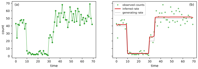
fig_29_6. Download: PDF · SVG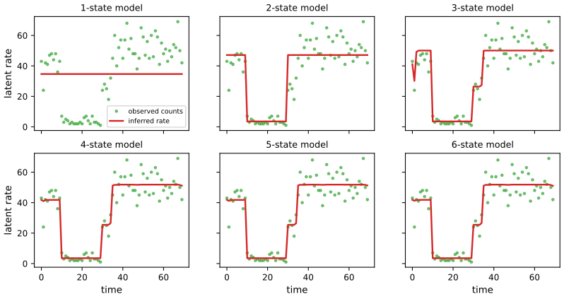
fig_29_7. Download: PDF · SVG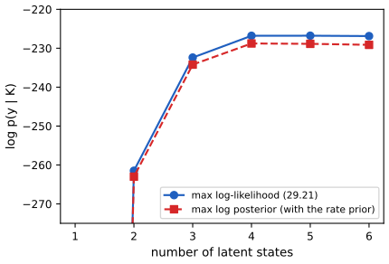
fig_29_8. Download: PDF · SVG29.3.2 Protein sequence alignment
pp. 1020–1022, Figures 29.9–29.10 A profile HMM turns a position-specific scoring matrix \(\theta_t(v)=p(y_t=v)\) into a three-state-per-position chain: match (emit from the PSSM), insert (emit uniformly, self-loop) and delete (emit a gap symbol), with matches and deletions advancing one position and insertions staying put. The forwards algorithm gives \(p(\vy_{1:T}\given\bm\theta)\) in \(O(T)\) (per consensus length), thresholding the log-odds \(\log p(\vy\given\bm\theta)/p(\vy\given M_0)\) decides family membership, and Viterbi gives the alignment; unaligned training sequences are handled with Baum–Welch (Section 29.4.1). The two figures are a diagram and a published alignment, and are not redrawn.
29.3.3 Spelling correction
pp. 1022–1024, (29.22) Let \(z_t\) be the intended word and \(y_t\) the typed word. The baseline treats words as independent, \(p(z_{1:T})=\prod_tp(z_t)\), with a noisy-channel likelihood that depends on the edit distance \(d\) between \(y\) and \(z\): \(p(y\given z)=p_1,p_2,p_3,p_4\) for \(d=0,1,2\) and larger, with \(p_1>p_2>p_3>p_4\) (29.22). Replacing the unigram prior by a bigram language model \(p(z_t\given z_{t-1})\) gives an HMM whose \(N\) best paths come from the \(N\)-best Viterbi algorithm in \(O(NTK^2)\); sparsity of \(p(y\given z)\) keeps the candidate lists short. Silent states let the extended model merge two words or split one. Because the likelihood is a function of the edit distance only, the baseline cannot learn that "reciet" is more often meant as "receipt" than "recite"; learning the channel from (correction, typo) pairs fixes this.
29.4 HMMs: parameter learning
p. 1024 Given partially observed sequences, we want a point estimate or the posterior of \(\bm\theta=(\bm\pi,\mathbf A,\mathbf B)\).
29.4.1 The Baum–Welch (EM) algorithm
pp. 1024–1027, (29.23)–(29.35), Algorithm 29.1 The complete-data likelihood of one sequence is
\[ p(\vy_{1:T},z_{1:T}\given\bm\theta)=p(z_1\given\bm\pi)\prod_{t=2}^{T}p(z_t\given z_{t-1},\mathbf A)\prod_{t=1}^{T}p(\vy_t\given z_t,\mathbf B), \tag{29.23} \]and EM maximises
\[ Q(\bm\theta,\bm\theta^{\mathrm{old}})=\E_{p(z_{1:T}\given\vy_{1:T},\bm\theta^{\mathrm{old}})}\big[\log p(\vy_{1:T},z_{1:T}\given\bm\theta)\big]. \tag{29.25} \]The E step runs forwards–backwards for each of the \(N\) sequences and collects the node and edge marginals \(\gamma_{n,t}(j)=p(z_t=j\given\vy_{n,1:T_n},\bm\theta^{\mathrm{old}})\) and \(\xi_{n,t}(j,k)=p(z_{t-1}=j,z_t=k\given\cdots)\) (29.26)–(29.27). The expected counts (29.28) are \(\E[N^1_k]=\sum_n\gamma_{n,1}(k)\), \(\E[N_k]=\sum_n\sum_t\gamma_{n,t}(k)\), \(\E[N_{jk}]=\sum_n\sum_{t\ge2}\xi_{n,t}(j,k)\). The M step normalises them:
\[ \hat A_{jk}=\frac{\E[N_{jk}]}{\sum_{k'}\E[N_{jk'}]},\quad \hat\pi_k=\frac{\E[N_k^1]}{N},\qquad \hat B_{kv}=\frac{\E[M_{kv}]}{\E[N_k]}, \tag{29.30, 29.32} \]with \(\E[M_{kv}]=\sum_{n,t}\gamma_{n,t}(k)\,\mathbb I(y_{n,t}=v)\) (29.31); for Gaussian emissions \(\hat{\bmu}_k=\E[\vy]_k/\E[N_k]\) and \(\hat{\bSig}_k=\E[\vy\vy^\T]_k/\E[N_k]-\hat{\bmu}_k\hat{\bmu}_k^\T\) (29.34)–(29.35). The sum defining \(\E[N_k]\) in (29.32) must run over all \(t\geq1\) (the book's (29.28) and Algorithm 29.1 start at \(t=2\), which makes the rows of \(\hat{\mathbf B}\) sum to more than one).
Filling the gap 29.3: EM for HMMs, the M step and the fixed point of identical states pp. 1024–1027, (29.25)–(29.35)
The book states that \(Q\) is a lower bound and gives the closed-form M step "intuitively". Here are the bound, the Lagrange-multiplier derivation, and two facts that explain the behaviour in the casino example (label switching and the symmetric fixed point).
Derivation
(i) EM never decreases the likelihood. For any \(\bm\theta\), with \(q=p(z\given\vy,\bm\theta^{\mathrm{old}})\), Jensen's inequality gives
\[ \log p(\vy\given\bm\theta)=\log\sum_zq(z)\frac{p(\vy,z\given\bm\theta)}{q(z)}\ \ge\ Q(\bm\theta,\bm\theta^{\mathrm{old}})+H(q), \]and equality holds at \(\bm\theta=\bm\theta^{\mathrm{old}}\) because \[ p(\vy,z\given\bm\theta^{\mathrm{old}})/q(z)=p(\vy\given\bm\theta^{\mathrm{old}}) \] is constant in \(z\). So \(\bm\theta^{\mathrm{new}}=\arg\max Q\) satisfies \[ \log p(\vy\given\bm\theta^{\mathrm{new}})\ge Q(\bm\theta^{\mathrm{new}},\cdot)+H\ge Q(\bm\theta^{\mathrm{old}},\cdot)+H=\log p(\vy\given\bm\theta^{\mathrm{old}}) \] (the general argument is in Section 6.5.3). (ii) The expected complete-data log-likelihood. Take the log of (29.24) and the expectation: \[ Q=\sum_k\E[N_k^1]\log\pi_k+\sum_{j,k}\E[N_{jk}]\log A_{jk}+\sum_{n,t,k}\gamma_{n,t}(k)\log p(\vy_{n,t}\given\bm\theta_k) \], which is (29.29): it separates into one term for \(\bm\pi\), one for each row of \(\mathbf A\), and one for each state's emission parameters. (iii) Normalised counts. Maximise \(\sum_kc_k\log x_k\) over the simplex \(\sum_kx_k=1\), \(c_k\ge0\): the Lagrangian \(\sum_kc_k\log x_k-\ell(\sum_kx_k-1)\) has stationarity \(c_k/x_k=\ell\); summing over \(k\), \(\ell=\sum_kc_k\), so \(x_k=c_k/\sum_{k'}c_{k'}\). Applied to \(\bm\pi\) (\(c_k=\E[N^1_k]\), total \(N\)), to row \(j\) of \(\mathbf A\) (\(c_k=\E[N_{jk}]\)) and to row \(k\) of \(\mathbf B\) (\(c_v=\E[M_{kv}]\), total \(\E[N_k]\) with the sum over all \(t\)) this gives (29.30) and (29.32). (iv) Gaussian emissions. With weights \(w_t=\gamma_t(k)\) and \(n_k=\sum_tw_t\), maximise \(\sum_tw_t\log\N(\vy_t\given\bmu,\bSig)\): the gradient in \(\bmu\) is \(\bSig^{-1}\sum_tw_t(\vy_t-\bmu)=0\), so \(\hat\bmu=\sum w_t\vy_t/n_k\); in \(\bSig^{-1}\) it is \(\tfrac12\sum_tw_t(\bSig-(\vy_t-\bmu)(\vy_t-\bmu)^\T)=0\), so \(\hat\bSig=\sum w_t(\vy_t-\hat\bmu)(\vy_t-\hat\bmu)^\T/n_k\), which expands to (29.35). With few effective points this is singular, hence the prior mentioned in the text.
(v) Label switching. Permuting the states, \(\bm\pi\to\bm\pi_\sigma\), \(\mathbf A\to\mathbf A_{\sigma\sigma}\), \(\mathbf B\to\mathbf B_\sigma\), leaves \(p(\vy\given\bm\theta)\) unchanged, so every maximum has \(K!\) copies; in Figure 29.13 EM and SGD recover the truth with the two states exchanged. (vi) A symmetric start is a fixed point. Suppose all rows of \(\mathbf B\) are equal and \(\bm\pi^\T\mathbf A=\bm\pi^\T\) (for example \(\mathbf A\) symmetric, \(\bm\pi\) uniform). Then \(\mathrm{lik}_t(k)\) does not depend on \(k\), so \(\bm\alpha_t=\bm\pi\), \(\bm\beta_t\propto\mathbf1\), \(\gamma_t(k)=\pi_k\) and \(\xi_t(j,k)=\pi_jA_{jk}\) for all \(t\). The M step returns the same \(\mathbf A\) and \(\bm\pi\) and sets every row of \(\mathbf B\) to the overall empirical distribution: again equal rows. The iteration never leaves this set, which is a saddle of the likelihood, not a maximum (preset 4 of the demonstration). ∎
29.4.1.4 Initialization
p. 1027 EM finds a local maximum, so the start matters: use labelled data if available, initialise the emissions by K-means or a mixture model that ignores the Markov structure, use random restarts, or use Viterbi training (replace the E step by the single most probable path), as a hard-assignment analogue of K-means. In our casino run a start with sticky random rows (\(0.7\mathbf I+0.3\) a random stochastic matrix) converges to the right optimum for all six seeds tried, while a start with fully random rows once settled in a poor optimum (average negative log-likelihood 1.7575 against 1.7419 at the best).
29.4.1.5 Example: casino HMM
p. 1027, Figure 29.13 We simulate 4 sequences of length 5000 (20,000 rolls) from the casino HMM, start from a random sticky model and run 200 EM iterations. The estimates are close to the truth with the states exchanged: stay probabilities 0.956 and 0.898 against 0.95 and 0.90, and \(P(\text{six})=0.518\) against 0.5 for the loaded die.
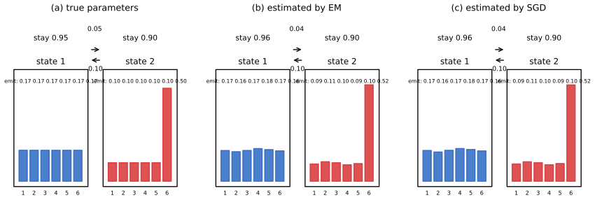
fig_29_13. Download: PDF · SVG29.4.2 Parameter estimation using SGD
pp. 1027–1028, (29.36)–(29.37), Figure 29.14 EM is a batch method. Alternatively minimise the negative log-likelihood \(-\log p(\vy_{1:T}\given\bm\theta)=-\sum_t\log Z_t\) with \(Z_t=\sum_jp(z_t=j\given\vy_{1:t-1})p(\vy_t\given z_t=j)\) (29.36)–(29.37) by (stochastic) gradient descent on an unconstrained parametrisation, for instance row-wise softmax for \(\mathbf A\) and \(\mathbf B\) and a Cholesky factor for \(\bSig\).
Filling the gap 29.4: the gradient of the HMM likelihood is the vector of expected counts p. 1028, (29.36)
The book differentiates the forwards recursion by automatic differentiation. One forwards–backwards pass gives the same gradient in closed form, which also explains why EM and gradient ascent are close relatives.
Derivation
Fisher's identity. For any model with latent \(z\), \[ \nabla_\theta\log p(\vy\given\theta)=\sum_z\frac{\nabla_\theta p(\vy,z\given\theta)}{p(\vy\given\theta)}=\sum_zp(z\given\vy,\theta)\,\nabla_\theta\log p(\vy,z\given\theta)=\nabla_\theta Q(\theta,\theta')\big|_{\theta'=\theta} \]. Softmax parametrisation. Let \(A_{jk}=e^{a_{jk}}/\sum_{k'}e^{a_{jk'}}\). Then \(\log p(\vy,z)\) contains \(N_{jk}(z)\log A_{jk}\) summed over \(j,k\), and \(\partial\log A_{jk}/\partial a_{jl}=\delta_{kl}-A_{jl}\), so \(\partial\log p(\vy,z)/\partial a_{jl}=N_{jl}(z)-A_{jl}N_{j\cdot}(z)\), where \(N_{j\cdot}=\sum_kN_{jk}\) counts the transitions out of \(j\). Averaging over \(p(z\given\vy)\):
\[ \frac{\partial\log p(\vy\given\bm\theta)}{\partial a_{jl}}=\E[N_{jl}]-A_{jl}\sum_k\E[N_{jk}],\qquad \frac{\partial\log p}{\partial b_{kv}}=\E[M_{kv}]-B_{kv}\E[N_k]. \]Similarly for \(\bm\pi\). The gradient vanishes exactly when the expected counts are proportional to the current parameters, i.e. at a fixed point of EM, so EM and gradient ascent share their stationary points. The code uses this formula (hmm_loglik_and_grad); it agrees with finite differences to \(10^{-6}\) and with PyTorch's reverse-mode gradient through the forwards algorithm to \(10^{-9}\). ∎
Example: casino HMM
On the same data as Figure 29.13 EM reaches within 0.001 of its final value of the average negative log-likelihood (1.7419, against 1.7424 at the true parameters, which the fit slightly beats) after 10 iterations, SGD with minibatch one needs about 100 passes to get there and does not decrease monotonically, and full-batch gradient descent with the same step size is still 0.0015 above the optimum after 200 steps. These are the qualitative findings of the text; the exact curves depend on step size and start.
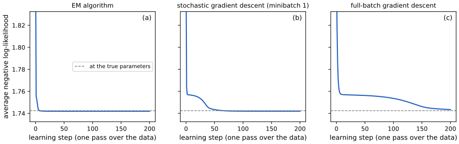
fig_29_14. Download: PDF · SVG29.4.3 Parameter estimation using spectral methods
pp. 1028–1029, (29.38)–(29.40) The likelihood of an HMM is not convex, so EM and SGD can land in poor local optima. The spectral alternative works with predictive distributions of the observations only. For a discrete HMM with \(m\) states and \(n\ge m\) symbols, the predictive state vectors \([\vy_t]_k=p(y_t=k\given\vy_{1:t-1})\) lie in an \(m\)-dimensional subspace of \(\R^n\); a basis for it comes from the SVD of the co-occurrence matrix \([\mathbf P_2]_{ij}=p(y_t=i,y_{t-1}=j)\) (29.39), and the update is completed with third-order statistics \(\mathbf P_3\) (29.40).
Filling the gap 29.5: why \(\mathbf P_2\) has rank \(m\) and how the observable operators reproduce the likelihood pp. 1028–1029, (29.38)–(29.40)
The book quotes Hsu, Kakade and Zhang (2012). Here is the argument, with the statistics written out for a stationary HMM. Let \(\mathbf O\in\R^{n\times m}\) with \(O_{vk}=p(y=v\given z=k)\), \(\mathbf T=\mathbf A^\T\) (so \(T_{kj}=p(z_{t+1}=k\given z_t=j)\), column stochastic), \(\bm\pi\) the stationary law (\(\mathbf T\bm\pi=\bm\pi\)), and \(\mathbf D_x=\operatorname{diag}(O_{x,\cdot})\). Assume \(\mathbf O\) and \(\mathbf T\) have rank \(m\) and \(\pi_k>0\).
Derivation
\[ \mathbf P_1=\mathbf O\bm\pi,\qquad \mathbf P_2=\mathbf O\mathbf T\operatorname{diag}(\bm\pi)\mathbf O^\T,\qquad \mathbf P_{3,x}=\mathbf O\mathbf T\mathbf D_x\mathbf T\operatorname{diag}(\bm\pi)\mathbf O^\T, \]where \([\mathbf P_2]_{ij}=p(y_2=i,y_1=j)\) and \([\mathbf P_{3,x}]_{ij}=p(y_3=i,y_2=x,y_1=j)\), by summing over the hidden states. Rank. \(\mathbf P_2\) is a product through \(\R^m\), so its rank is at most \(m\); with the full-rank assumptions it equals \(m\), and the range of \(\mathbf P_2\) is the range of \(\mathbf O\mathbf T\), which is why a basis \(\mathbf U\in\R^{n\times m}\) of the top-\(m\) left singular vectors identifies it. Put \(\mathbf S=\mathbf U^\T\mathbf O\) (invertible, as \(\mathbf U^\T\mathbf O\mathbf T\) is). Operators. With \(\mathbf N=\operatorname{diag}(\bm\pi)\mathbf O^\T\) (full row rank, so \(\mathbf N\mathbf N^+=\mathbf I\)), \(\mathbf U^\T\mathbf P_2=\mathbf S\mathbf T\mathbf N\) and \((\mathbf U^\T\mathbf P_2)^+=\mathbf N^+\mathbf T^{-1}\mathbf S^{-1}\), hence
\[ \mathbf B_x:=(\mathbf U^\T\mathbf P_{3,x})(\mathbf U^\T\mathbf P_2)^+=\mathbf S\mathbf T\mathbf D_x\mathbf T\mathbf N\mathbf N^+\mathbf T^{-1}\mathbf S^{-1}=\mathbf S\,\mathbf T\mathbf D_x\,\mathbf S^{-1}. \]Also \(\mathbf b_1:=\mathbf U^\T\mathbf P_1=\mathbf S\bm\pi\) and \[ \mathbf b_\infty:=(\mathbf P_2^\T\mathbf U)^+\mathbf P_1=\mathbf S^{-\T}\mathbf T^{-\T}\mathbf1=\mathbf S^{-\T}\mathbf1 \], using \(\mathbf1^\T\mathbf T=\mathbf1^\T\). Multiplying,
\[ \mathbf b_\infty^\T\mathbf B_{y_t}\cdots\mathbf B_{y_1}\mathbf b_1=\mathbf1^\T\mathbf T\mathbf D_{y_t}\mathbf T\mathbf D_{y_{t-1}}\cdots\mathbf T\mathbf D_{y_1}\bm\pi=\mathbf1^\T\mathbf D_{y_t}\mathbf T\mathbf D_{y_{t-1}}\cdots\mathbf T\mathbf D_{y_1}\bm\pi=p(y_1,\dots,y_t), \]the last form being the forwards algorithm unrolled. So the \(m\times m\) matrices \(\mathbf B_x\), estimable from observable statistics alone, update a predictive state exactly. The code compares \(p(y_{1:5})\) from these operators with the forwards algorithm on random HMMs (\(n=6,m=3\)) to \(10^{-10}\). With empirical \(\hat{\mathbf P}\) the same formulas give consistent estimators, and the result can start EM. ∎
29.4.4 Bayesian HMMs
p. 1029 MLE can overfit and be numerically fragile. Bayesian options: a hierarchical Dirichlet process prior for an unbounded number of states (HDP-HMM), variational Bayes EM, blocked Gibbs sampling, or the collapsed approach of marginalising the discrete states with the forwards algorithm and running HMC or SVI on \[ \log p(\bm\theta,\mathcal D)=\log p(\bm\theta)+\sum_n\log p(\vy_{1:T,n}\given\bm\theta) \] (29.41), which avoids the slow mixing caused by the strong correlation between \(\vz\) and \(\bm\theta\).
29.4.4.1 Blocked Gibbs sampling for HMMs
pp. 1030–1031, (29.42)–(29.49) For the AR-HMM with known offsets \(\bmu_j\), alternate between sampling \(z_{1:T}\) by forwards filtering, backwards sampling (Section 9.2.7) and sampling \(\bm\theta\) from its conjugate full conditional. The priors are \(\bm\pi\sim\mathrm{Dir}(\breve\alpha_\pi/K)\), \(\mathbf A_{j\cdot}\sim\mathrm{Dir}(\breve\alpha_A/K)\), \(\bSig_j\sim\mathrm{IW}(\breve\nu_j,\breve\bPsi_j)\), \[ \mathbf E_j\given\bSig_j\sim\mathrm{MN}(\breve{\mathbf M}_j,\bSig_j,\breve{\mathbf V}_j) \] (29.42)–(29.43), and the posteriors are
\[ \bm\pi\given z\sim\mathrm{Dir}(\breve\alpha_\pi/K+\mathbb I(z_1=k)),\quad \mathbf A_{j\cdot}\given z\sim\mathrm{Dir}(\breve\alpha_A/K+N_{jk}),\quad \bSig_j,\mathbf E_j\ \text{matrix-normal inverse Wishart}. \tag{29.47–29.49} \]Filling the gap 29.6: the conjugate updates of the Gibbs sampler pp. 1030–1031, (29.44)–(29.49)
The Dirichlet update is a one-line product of kernels; the matrix-normal inverse-Wishart update (which the book defers to its Section 15.2.9) is a completion of squares, written out here for the AR coefficients of one state.
Derivation
Transitions. Given \(z_{1:T}\), the likelihood of row \(j\) of \(\mathbf A\) is \(\prod_kA_{jk}^{N_{jk}}\) and the prior kernel is \(\prod_kA_{jk}^{\breve\alpha_A/K-1}\); the product is the kernel of \(\mathrm{Dir}(\breve\alpha_A/K+N_{jk})\). The same holds for \(\bm\pi\) with the single count \(\mathbb I(z_1=k)\). Directly: for \(K=2\) the posterior mean \((\alpha/2+N_{j1})/(\alpha+N_j)\) agrees with numerical integration (confirmed).
Regression coefficients. For the \(N_j\) steps in state \(j\) stack \(\hat{\mathbf Y}\in\R^{N_j\times N_y}\) with rows \((\vy_t-\bmu_j)^\T\) and \(\tilde{\mathbf Y}\) with rows \(\vy_{t-1}^\T\), so that \(\hat{\mathbf Y}^\T=\mathbf E\tilde{\mathbf Y}^\T+\)noise with columns \(\N(\mathbf0,\bSig)\). The likelihood is, up to a constant, \[ |\bSig|^{-N_j/2}\exp\{-\tfrac12\operatorname{tr}\bSig^{-1}(\hat{\mathbf Y}^\T-\mathbf E\tilde{\mathbf Y}^\T)(\hat{\mathbf Y}^\T-\mathbf E\tilde{\mathbf Y}^\T)^\T\} \]; the prior \(\mathbf E\given\bSig\sim\mathrm{MN}(\mathbf M,\bSig,\mathbf V)\) contributes \[ |\bSig|^{-N_y/2}\exp\{-\tfrac12\operatorname{tr}\bSig^{-1}(\mathbf E-\mathbf M)\mathbf V^{-1}(\mathbf E-\mathbf M)^\T\} \], and \(\bSig\sim\mathrm{IW}(\nu,\bPsi)\) contributes \(|\bSig|^{-(\nu+N_y+1)/2}e^{-\frac12\operatorname{tr}\bSig^{-1}\bPsi}\). Collect everything inside \(\operatorname{tr}\bSig^{-1}[\cdots]\):
\[ \mathbf E(\tilde{\mathbf Y}^\T\tilde{\mathbf Y}+\mathbf V^{-1})\mathbf E^\T-\mathbf E(\tilde{\mathbf Y}^\T\hat{\mathbf Y}+\mathbf V^{-1}\mathbf M^\T)-(\cdot)^\T\mathbf E^\T+\hat{\mathbf Y}^\T\hat{\mathbf Y}+\mathbf M\mathbf V^{-1}\mathbf M^\T+\bPsi. \]Define \(\mathbf V_n^{-1}=\mathbf V^{-1}+\tilde{\mathbf Y}^\T\tilde{\mathbf Y}\) and \[ \mathbf M_n=(\hat{\mathbf Y}^\T\tilde{\mathbf Y}+\mathbf M\mathbf V^{-1})\mathbf V_n \]. Completing the square in \(\mathbf E\) gives \[ (\mathbf E-\mathbf M_n)\mathbf V_n^{-1}(\mathbf E-\mathbf M_n)^\T+\bPsi_n \] with \[ \bPsi_n=\bPsi+\hat{\mathbf Y}^\T\hat{\mathbf Y}+\mathbf M\mathbf V^{-1}\mathbf M^\T-\mathbf M_n\mathbf V_n^{-1}\mathbf M_n^\T \] (the algebraic identity is confirmed numerically on random matrices). The power of \(|\bSig|\) is \(-(\nu+N_j+N_y+1)/2-N_y/2\), so \(\bSig\given\text{data}\sim\mathrm{IW}(\nu+N_j,\bPsi_n)\) and \[ \mathbf E\given\bSig,\text{data}\sim\mathrm{MN}(\mathbf M_n,\bSig,\mathbf V_n) \]. The LDS sampler of Section 29.8.4.1 is the same computation with \(\hat{\mathbf Y}=\) the sampled states (or observations) and \(\tilde{\mathbf Y}=\) the regressors \((\vz_{t-1},\vu_t)\). ∎
29.5 HMMs: generalizations
29.5.1 Hidden semi-Markov model (HSMM)
pp. 1031–1033, (29.50)–(29.57) In an HMM the time spent in state \(i\) is geometric. Counting \(d\ge1\) steps (the book's (29.50) has an exponent \(d\) instead of \(d-1\)), \(p(d_i=d)=(1-A_{ii})A_{ii}^{d-1}\), with mean \(1/(1-A_{ii})\) and mode at \(d=1\). Two ways to get other waiting times: replace each state by a chain of \(n\) copies, or make the duration an explicit variable \(d_t\) that counts down. Figure 29.15 shows the first approach, which gives the negative binomial law
\[ p(d)=\binom{d-1}{n-1}p^{\,d-n}(1-p)^n,\quad d\ge n. \tag{29.51} \]Filling the gap 29.7: the duration of \(n\) chained states is negative binomial p. 1031, (29.50)–(29.51)
The book derives (29.51) by counting paths; here is the sum-of-geometrics view, with its mean and variance.
Derivation
Each of the \(n\) states is occupied for a geometric number of steps \(G_i\) with \(P(G_i=g)=p^{g-1}(1-p)\), \(g\ge1\), independently, so the total duration is \(D=G_1+\dots+G_n\). A path of total length \(d\) takes \(n\) exits (probability \((1-p)^n\)) and \(d-n\) self-loops (\(p^{d-n}\)), regardless of how the \(d-n\) self-loops are distributed among the \(n\) states; the number of ways to split \(d\) steps into \(n\) positive parts is \(\binom{d-1}{n-1}\) (place \(n-1\) cut points among the \(d-1\) gaps). This is (29.51). Since \(\E G_i=1/(1-p)\) and \(\var G_i=p/(1-p)^2\), \(\E D=n/(1-p)\) and \(\var D=np/(1-p)^2\). For \(p=0.99\): means 100, 200, 500 for \(n=1,2,5\) (Figure 29.15) and standard deviations 99.5, 140.7, 222.5; the larger \(n\) the more the law concentrates around its mean relative to the geometric. The pmf sums to 1 and equals the negative binomial pmf with \(n\) successes and success probability \(1-p\) shifted by \(n\) (confirmed numerically, and by simulating the chain). ∎
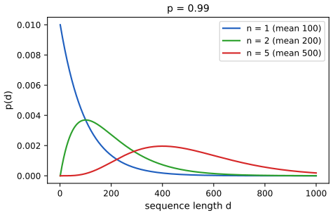
fig_29_15. Download: PDF · SVGThe explicit-duration model draws \(d_t\sim D_j(\cdot)\) when state \(j\) is entered and counts down: \(p(d_t=d'\given d_{t-1}=d,z_t=j)=D_j(d')\) if \(d=1\), \(=1\) if \(d'=d-1>0\) (29.52), and the state is frozen while \(d_t>1\) (29.53). With \(D_j\) a truncated geometric this is an ordinary HMM. A segmental HMM further lets a whole segment of \(l\) observations be emitted jointly, \(p(\vy_{t:t+l-1}\given z_t=k,d_t=l)\) (29.54)–(29.57), for example by an RNN per segment. Exact inference over \((z_t,d_t)\) costs \(O(TK^2+TKD)\) with maximum duration \(D\).
29.5.2 Hierarchical HMMs
pp. 1033–1035, Figures 29.17–29.18 A hierarchical HMM has states that are themselves HMMs (words made of phones made of subphones). It can always be flattened to an HMM, but the factored form is easier to interpret and to fit. A chain at level \(\ell\) may transition only when the chain below has finished (flag \(F^{\ell-1}_t=1\)), so higher levels change more slowly. Inference is \(O(T)\), against \(O(T^3)\) for stochastic context-free grammars via inside–outside, because the depth is bounded. A variable-duration HMM is the special case with a deterministic counter on top.
29.5.3 Factorial HMMs
pp. 1035–1036, (29.58)–(29.61), Figure 29.19a To represent 10 bits an HMM needs \(K=1024\) states; a factorial HMM uses \(M\) independent binary (or \(K\)-ary) chains, \[ p(\vz,\vy)=\prod_t\big[\prod_mp(z_{tm}\given z_{t-1,m})\big]p(\vy_t\given\vz_t) \] with \(p(\vy_t\given\vz_t)=\N(\vy_t\given\sum_m\mathbf W_m\vz_{tm},\bSig)\) (29.58)–(29.59). In energy disaggregation the observation is the total power \(\N(\sum_mw_mz_{tm},\sigma^2)\) of \(M\) devices (29.60). Given \(\vy_t\) all chains are coupled (explaining away), so exact inference costs \(O(TK^{2M})\) and one resorts to variational approximations.
29.5.4 Coupled HMMs
p. 1036, (29.62) Coupled HMMs let each chain's transition depend on its neighbours, \[ p(\vz_t,\vy_t\given\vz_{t-1})=\prod_mp(y_{tm}\given z_{tm})p(z_{tm}\given z_{t-1,m-1:m+1}) \]. Exact inference costs \(O(T K^{2M})\) as for the factorial HMM, and the table of a chain with two neighbours has \(O(K^4)\) entries (the book writes \(O(MK^4)\) in total); the influence model reduces parameters by a convex combination of pairwise tables.
29.5.5 Dynamic Bayes nets (DBN)
p. 1037, Figure 29.20 A DBN represents a stochastic process with a directed graph repeated in time: specify the first slice, the structure between two slices and the conditional distributions. It generalises the HMM, and the example network monitors a simulated autonomous car. (The structure is fixed; only the variables are indexed by time.)
29.5.6 Changepoint detection
pp. 1037–1040, (29.63)–(29.72) The task is to detect, online, abrupt changes in the distribution of a series. Instead of the duration counting down, track the run length \(r_t\in\{0,1,\dots\}\), the number of earlier observations in the current segment: \(r_t=0\) when a new segment starts and otherwise \(r_t=r_{t-1}+1\), with the transition
\[ p(r_t\given r_{t-1})=\begin{cases}H(r_{t-1}+1)&r_t=0\\ 1-H(r_{t-1}+1)&r_t=r_{t-1}+1\\0&\text{otherwise}\end{cases}\tag{29.63} \]where \(H\) is the hazard function \(H(\tau)=p_g(\tau)/\sum_{t\ge\tau}p_g(t)\) for the segment-length law \(p_g\) (29.64): a geometric \(p_g\) with mean \(\lambda\) gives the constant hazard \(1/\lambda\). In a segment with run length \(r\) the observation is predicted from the last \(r\) observations through the underlying predictive model (UPM),
\[ p(y_t\given y_{1:t-1},r_t=r)=p(y_t\given y_{t-r:t-1})=\int p(y_t\given\eta)\,p(\eta\given y_{t-r:t-1})\,\d\eta, \tag{29.65–29.67} \]closed form for conjugate exponential families. Setting \(K=1\) recovers the product partition model (29.68): independent segments with no information sharing. The exact online algorithm (Fearnhead and Liu 2007; Adams and MacKay 2007: Bayesian online changepoint detection, BOCPD) is the recursion
\[ p(r_t\given\vy_{1:t})\propto p(\vy_t\given\vy_{1:t-1},r_t)\,p(r_t\given\vy_{1:t-1}),\qquad p(r_t\given\vy_{1:t-1})=\sum_{r_{t-1}}p(r_t\given r_{t-1})p(r_{t-1}\given\vy_{1:t-1}), \tag{29.69–29.70} \]with \(p(r_0=0)=1\) (our code starts the first segment at \(r_1=0\)), and the predictive \[ p(\vy_{t+1}\given\vy_{1:t})=\sum_{r_t}p(\vy_{t+1}\given\vy_{1:t},r_t)p(r_t\given\vy_{1:t}) \] (29.71).
Filling the gap 29.8: why the BOCPD recursion is exact, the hazard, and the Gaussian predictive pp. 1038–1039, (29.63)–(29.71)
The book cites the papers. The two facts to prove are that the run-length process is Markov and independent of the data, and that, given \(r_t\), the new observation depends on the past only through the last \(r_t\) observations.
Derivation
Model. Draw the run lengths from the Markov chain (29.63). Given the run-length path, the observations in different segments are independent, and within a segment, with parameter \(\eta\) drawn fresh from its prior at the segment start, they are conditionally iid given \(\eta\). Equivalently, the joint density of \(\vy_{1:T}\) given a segmentation is the product over segments of the marginal likelihoods \(p(\vy_{s_i:e_i})=\int\prod_{t}p(y_t\given\eta)p(\eta)\,\d\eta\) (29.68). Recursion. Write \(p(r_t,\vy_{1:t})=\sum_{r_{t-1}}p(r_t,r_{t-1},\vy_{t},\vy_{1:t-1})\) and factor \[ p(r_t,r_{t-1},\vy_{1:t})=p(y_t\given r_t,r_{t-1},\vy_{1:t-1})\,p(r_t\given r_{t-1},\vy_{1:t-1})\,p(r_{t-1},\vy_{1:t-1}). \] (a) \(p(r_t\given r_{t-1},\vy_{1:t-1})=p(r_t\given r_{t-1})\): the run-length chain does not look at the data. (b) If \(r_t=r>0\) then \(r_{t-1}=r-1\) is determined, and \(y_t\) belongs to the segment that began at \(t-r\), so by conditional iid-ness \(p(y_t\given r_t=r,\vy_{1:t-1})=p(y_t\given\vy_{t-r:t-1})\), the UPM predictive; observations before \(t-r\) belong to other segments and are independent of \(\eta\). If \(r_t=0\), \(y_t\) is the first observation of a new segment and has the prior predictive whatever \(r_{t-1}\) was. So the likelihood factor depends on \(r_t\) only, and summing over \(r_{t-1}\) gives \[ p(r_t,\vy_{1:t})=p(y_t\given\vy_{t-r_t:t-1})\sum_{r_{t-1}}p(r_t\given r_{t-1})p(r_{t-1},\vy_{1:t-1}) \]; normalising by \(p(\vy_t\given\vy_{1:t-1})\) gives (29.69)–(29.70). Summing over \(r_t\) yields the one-step predictive (29.71) and \(\log p(\vy_{1:T})=\sum_t\log p(y_t\given\vy_{1:t-1})\). Hazard. If a segment has length law \(p_g\), the probability that it ends after exactly \(\tau\) steps given that it has reached \(\tau\) is \(p_g(\tau)/P(\text{length}\ge\tau)=H(\tau)\) (29.64); for \(p_g(\tau)=\lambda(1-\lambda)^{\tau-1}\) the numerator and tail are \(\lambda(1-\lambda)^{\tau-1}\) and \((1-\lambda)^{\tau-1}\), so \(H\equiv\lambda\). Gaussian UPM. With \(y\given\mu\sim\N(\mu,s^2)\) and \(\mu\sim\N(\mu_0,v_0)\), after \(n\) observations with sum \(S\) the posterior is \(\N(m_n,v_n)\), \(v_n=(1/v_0+n/s^2)^{-1}\), \(m_n=v_n(\mu_0/v_0+S/s^2)\), and the predictive is \(\N(m_n,v_n+s^2)\); the sufficient statistics \((n,S)\) update in \(O(1)\), so one step costs \(O(t)\) and the whole run \(O(T^2)\). Check. For \(T=7\) the evidence and the run-length posterior from the recursion agree with a brute-force sum over all \(2^{T-1}\) segmentations to \(10^{-9}\), and the predictive equals the ratio of Gaussian marginal likelihoods. A remark on reading the output. In this convention the posterior mass of a new segment appears first at \(r_t=0\) only if the new observation is clearly out of place under the old segment; a moderate shift is first seen as mass on \(r_t=1,2,3,\dots\) as evidence accumulates. That is why the changepoint probability \(p(r_t=0\given\vy_{1:t})\) peaks at only 0.32 and 0.20 at two of our four changepoints, while the run-length image shows each reset clearly and the most probable run length locates all four. ∎
Example (p. 1039, Figure 29.22). The book uses a Gaussian UPM with known variance on 200 observations from a 4-state Gaussian mixture with geometric hazard of rate \(N/T\). We simulate a series of length 200 with unit-variance noise and four changepoints at 45, 80, 130, 160 (means \(0,3.2,-1.5,2.5,-3\)), hazard \(H=4/200\), prior \(\N(0,4)\) and noise variance 1. Reading the changepoint locations off the most probable run length (a reset followed by the start of the settled segment 10 steps later) recovers exactly 45, 80, 130, 160, and the log evidence is \(-320.8\), against \(-282.4\) for pure noise of the same length (nothing to explain).
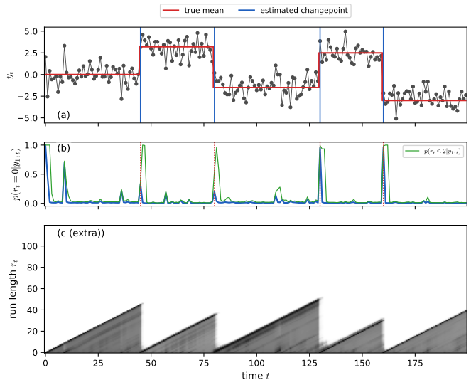
fig_29_22. Download: PDF · SVG29.6 Linear dynamical systems (LDSs)
pp. 1040–1041, (29.73)–(29.80) The linear dynamical system (LDS, or linear-Gaussian SSM) has linear transition and observation functions with Gaussian noise. The conditional independence structure is that of Figure 29.1: hidden Markov states, observations independent given the states.
29.6.1 Conditional independence properties
p. 1040 As for the HMM, the states are Markov and the observations are conditionally independent given the states; only the form of the conditional distributions remains to be given.
29.6.2 Parameterization
pp. 1040–1041
\[ p(\vz_t\given\vz_{t-1},\vu_t)=\N(\vz_t\given\mF_t\vz_{t-1}+\mathbf B_t\vu_t+\mathbf b_t,\mQ_t),\qquad p(\vy_t\given\vz_t,\vu_t)=\N(\vy_t\given\mH_t\vz_t+\mathbf D_t\vu_t+\mathbf d_t,\mR_t), \tag{29.73–29.74} \]and, dropping offsets and inputs, \(\vz_t=\mF_t\vz_{t-1}+\mathbf q_t\), \(\vy_t=\mH_t\vz_t+\mathbf r_t\) with \(\mathbf q_t\sim\N(\mathbf0,\mQ_t)\), \(\mathbf r_t\sim\N(\mathbf0,\mR_t)\) (29.79)–(29.80). Parameters are usually constant in time (a stationary model). Online inference is the Kalman filter and offline inference the Kalman smoother, proved in Result 8.1 and Result 8.2 of this course (and in Result 13.30 of the Bishop-notation course); the code kalman_filter, rts_smoother of this chapter is a short stand-alone implementation that matches brute-force conditioning of the joint Gaussian to \(10^{-9}\).
29.7 LDS: applications
29.7.1 Object tracking and state estimation
pp. 1041–1043, (29.81)–(29.82), Figure 29.23 Let the state be the position and velocity of an object in the plane, \(\vz_t=(u_t,v_t,\dot u_t,\dot v_t)\). Newton's law with a white-noise random acceleration, observed at times separated by \(\Delta\), gives
\[ \vz_t=\begin{pmatrix}1&0&\Delta&0\\0&1&0&\Delta\\0&0&1&0\\0&0&0&1\end{pmatrix}\vz_{t-1}+\mathbf q_t,\quad \mathbf q_t\sim\N(\mathbf0,\mQ),\ \ \mQ=\begin{pmatrix}q_1\Delta^3/3&0&q_1\Delta^2/2&0\\0&q_2\Delta^3/3&0&q_2\Delta^2/2\\q_1\Delta^2/2&0&q_1\Delta&0\\0&q_2\Delta^2/2&0&q_2\Delta\end{pmatrix}, \tag{29.81} \]and the sensor reports the position plus noise, \(\vy_t=\mH\vz_t+\mathbf r_t\), \(\mathbf r_t\sim\N(\mathbf0,\mathrm{diag}(\sigma_1^2,\sigma_2^2))\) (29.82). The book's \(\mH\) in (29.82) is printed as \(\begin{pmatrix}1&0&0&0\\0&0&1&0\end{pmatrix}\), which extracts \((u,\dot u)\) from the state ordered as \((u,\dot u,v,\dot v)\) and not from the ordering of (29.81); with (29.81)'s ordering it must be \(\begin{pmatrix}1&0&0&0\\0&1&0&0\end{pmatrix}\), as in our code. Filtering with a vague prior \(\N(\mathbf0,10^5\mI)\) gives estimates with large ellipses; smoothing uses later data and shrinks them. Figure 29.23 is Figure 8.2 repeated: it is reproduced in Chapter 8, Figure 8.2 and in the Kalman filter demonstration, not redrawn here.
Filling the gap 29.9: the discretised white-noise-acceleration covariance p. 1042, (29.81)
The book gives \(\mQ\) with a reference. It is the covariance of the stochastic integral of a continuous-time model, and the entries \(\Delta^3/3\), \(\Delta^2/2\), \(\Delta\) come from integrating \(s^2\), \(s\), \(1\).
Derivation
The continuous-time model is \(\d\vz=\mathbf F_c\vz\,\d t+\mathbf L\,\d\mathbf W\) with \[ \mathbf F_c=\begin{pmatrix}\mathbf0&\mI_2\\\mathbf0&\mathbf0\end{pmatrix} \] (position integrates velocity), \(\mathbf L=\begin{pmatrix}\mathbf0\\\mI_2\end{pmatrix}\) (the noise drives the velocity: acceleration is white noise) and \(\mathbf W\) a Brownian motion with diffusion matrix \(\mQ_c=\mathrm{diag}(q_1,q_2)\). The solution over one interval is \[ \vz_t=e^{\mathbf F_c\Delta}\vz_{t-1}+\int_0^\Delta e^{\mathbf F_c(\Delta-s)}\mathbf L\,\d\mathbf W_s \], and by the Ito isometry the noise has covariance \[ \mQ=\int_0^\Delta e^{\mathbf F_cs}\mathbf L\mQ_c\mathbf L^\T e^{\mathbf F_c^\T s}\,\d s \]. Because \(\mathbf F_c^2=\mathbf0\), \[ e^{\mathbf F_cs}=\mI+s\mathbf F_c=\begin{pmatrix}\mI&s\mI\\\mathbf0&\mI\end{pmatrix} \], and \(e^{\mathbf F_cs}\mathbf L=\begin{pmatrix}s\mI\\\mI\end{pmatrix}\). For coordinate \(i\) the integrand is \(q_i\begin{pmatrix}s^2&s\\s&1\end{pmatrix}\), whose integral over \([0,\Delta]\) is \[ q_i\begin{pmatrix}\Delta^3/3&\Delta^2/2\\\Delta^2/2&\Delta\end{pmatrix} \], which with the state ordering \((u,v,\dot u,\dot v)\) is the matrix in (29.81). The transition matrix is \(e^{\mathbf F_c\Delta}=\mI+\Delta\mathbf F_c\), the matrix (29.81). Confirmed numerically against the Van Loan matrix-exponential formula for the integral. ∎
29.7.2 Online Bayesian linear regression (recursive least squares)
pp. 1042–1044, (29.83)–(29.86), Figure 29.24 Sequential Bayesian updating \[ p(\vw\given\mathcal D_{1:t})\propto p(\mathcal D_t\given\vw)p(\vw\given\mathcal D_{1:t-1}) \] (29.83)–(29.84) is a Kalman filter in which the hidden state is the weight vector: \(p(\vy_t\given\vw_t)=\N(y_t\given\vx_t^\T\vw_t,\sigma^2)\) means \(\mH_t=\vx_t^\T\) (a time-varying observation matrix), and fixed weights mean \(\mF=\mI\), \(\mQ=\mathbf0\), i.e. \(p(\vw_t\given\vw_{t-1})=\delta(\vw_t-\vw_{t-1})\) (29.85)–(29.86). The derivation of the simplified gain, \(\mK_t=\bSig_{t-1}\vx_t/(\sigma^2+\vx_t^\T\bSig_{t-1}\vx_t)\), is Supplement 8.1.2 of this course. Letting \(\mQ\ne\mathbf0\) gives a dynamic linear model with drifting weights. Two remarks. First, after the last data point the filter equals the batch posterior (a one-pass algorithm; confirmed to \(10^{-9}\)). Second, the least-mean-squares (LMS) update \(\vw\leftarrow\vw+\eta_t(y_t-\vx_t^\T\vw)\vx_t\) is obtained by replacing \(\bSig_{t-1}/(\sigma^2+\vx_t^\T\bSig_{t-1}\vx_t)\) by a scalar \(\eta_t\), i.e. the gain is \(\eta_t\vx_t\) (the book writes \(\mK_t\approx\eta_t\mathbf1\), which does not give LMS); RLS adapts the step size per direction automatically. Footnote 3 of the book is right that the covariates cannot be passed as the input \(\vu_t\): the input term is \(\mathbf D\vu_t\) with \(\mathbf D\) a fixed parameter, whereas the weights have to be the state.
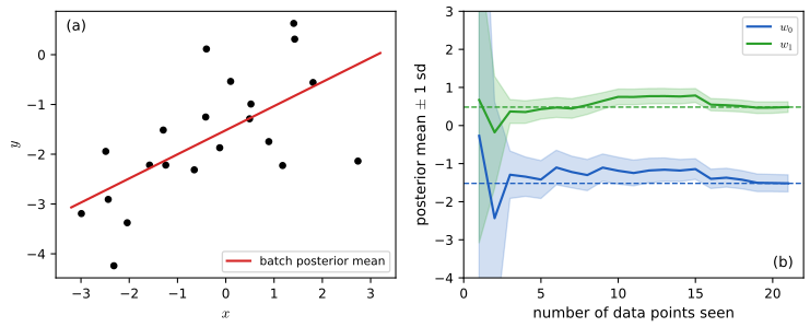
fig_29_24. Download: PDF · SVG29.7.3 Adaptive filtering
p. 1044, (29.87) For the AR(\(D\)) model \(y_t=w_1y_{t-1}+\dots+w_Dy_{t-D}+\epsilon_t\), put the coefficients in the state, \(\vz_t=\vw\), with \(\mH_t=(y_{t-1},\dots,y_{t-D})\); this is RLS with past observations as the regressors, and letting \(\vw\) drift adapts to a changing process.
29.7.4 Time series forecasting
p. 1044 See Section 29.12 below.
29.8 LDS: parameter learning
pp. 1045–1049 Estimating the parameters of an SSM is system identification in control. For LDSs the options mirror those for HMMs: EM, SGD (differentiate the Kalman-filter log-likelihood), spectral methods, and Bayesian inference.
29.8.1 EM for LDS
pp. 1045–1047, (29.88)–(29.108) As for HMMs, EM maximises \[ \E[\log p(\vz_{1:T},\vy_{1:T}\given\bm\theta)\given\vy_{1:T},\vu_{1:T},\bm\theta^{k-1}] \], with the Kalman smoother as E step: \(\hat{\vz}_t=\bmu_{t|T}\), \(\mathbf P_t=\bSig_{t|T}+\bmu_{t|T}\bmu_{t|T}^\T\) (29.92) and \(\mathbf P_{t,t-1}=\bSig_{t,t-1|T}+\bmu_{t|T}\bmu_{t-1|T}^\T\) (29.93). With the bias terms absorbed into \(\mathbf B,\mathbf D\) (a constant last entry of \(\vu_t\)) and the initial law \(\vz_1\sim\N(\mathbf m_1,\mathbf V_1)\), write \(\mathbf A_{\mathrm{out}}=[\mH,\mathbf D]\), \(\mathbf A_{\mathrm{dyn}}=[\mF,\mathbf B]\). The M step is
\[ \mathbf A^{\mathrm{new}}_{\mathrm{out}}=\Big(\sum_{t=1}^T\vy_t\hat{\vx}_{\mathrm{out},t}^\T\Big)\Big(\sum_{t=1}^T\mathbf P_{\mathrm{out},t}\Big)^{-1},\qquad \mR^{\mathrm{new}}=\frac1T\sum_{t=1}^T\big(\vy_t\vy_t^\T-\mathbf A^{\mathrm{new}}_{\mathrm{out}}\hat{\vx}_{\mathrm{out},t}\vy_t^\T\big), \tag{29.97, 29.99} \] \[ \mathbf A^{\mathrm{new}}_{\mathrm{dyn}}=\Big(\sum_{t=2}^T[\mathbf P_{t,t-1},\hat{\vz}_t\vu_t^\T]\Big)\Big(\sum_{t=2}^T\mathbf P_{\mathrm{dyn},t}\Big)^{-1},\quad \mQ^{\mathrm{new}}=\frac1{T-1}\sum_{t=2}^T\big(\mathbf P_t-\mathbf A^{\mathrm{new}}_{\mathrm{dyn}}[\mathbf P_{t-1,t},\vu_t\hat{\vz}_t^\T]\big), \tag{29.101, 29.104} \] \[ \mathbf m_1^{\mathrm{new}}=\hat{\vz}_1,\qquad \mathbf V_1^{\mathrm{new}}=\mathbf P_1-\hat{\vz}_1\hat{\vz}_1^\T. \tag{29.106, 29.108} \]Computing the statistics costs \(O(T)\) per iteration; the ASOS method precomputes second-order statistics to make later iterations independent of \(T\), and Kalman smoothing can be done in \(O(\log T)\) parallel time by associative scan (Section 8.2.3.4).
Filling the gap 29.10: the M step as a regression on expected statistics, and the lag-one covariance pp. 1045–1047, (29.89)–(29.108)
The book gets (29.97)–(29.108) by "standard matrix calculus". All four updates are one lemma, and the lag-one covariance (29.94) follows from Gaussian conditioning.
Derivation
Lemma (Gaussian regression from sufficient statistics). For targets \(\mathbf a_t\) and regressors \(\mathbf x_t\), the maximiser of \(\sum_{t=1}^n\E\log\N(\mathbf a_t\given\mathbf W\mathbf x_t,\mathbf C)\) over \(\mathbf W\) and positive definite \(\mathbf C\), with \(\mathbf S_{ax}=\sum\E[\mathbf a_t\mathbf x_t^\T]\), \(\mathbf S_{xx}=\sum\E[\mathbf x_t\mathbf x_t^\T]\), \(\mathbf S_{aa}=\sum\E[\mathbf a_t\mathbf a_t^\T]\), is \(\hat{\mathbf W}=\mathbf S_{ax}\mathbf S_{xx}^{-1}\), \[ \hat{\mathbf C}=\frac1n(\mathbf S_{aa}-\hat{\mathbf W}\mathbf S_{ax}^\T) \]. Proof. The objective is \[ -\frac n2\log|\mathbf C|-\frac12\operatorname{tr}\mathbf C^{-1}(\mathbf S_{aa}-\mathbf W\mathbf S_{ax}^\T-\mathbf S_{ax}\mathbf W^\T+\mathbf W\mathbf S_{xx}\mathbf W^\T) \]. Its gradient in \(\mathbf W\) is \(\mathbf C^{-1}(\mathbf S_{ax}-\mathbf W\mathbf S_{xx})\), zero at \(\hat{\mathbf W}\) for every \(\mathbf C\); at \(\hat{\mathbf W}\) the bracket equals \(\mathbf S_{aa}-\hat{\mathbf W}\mathbf S_{ax}^\T\) (using \[ \hat{\mathbf W}\mathbf S_{xx}\hat{\mathbf W}^\T=\mathbf S_{ax}\hat{\mathbf W}^\T \]), and the derivative in \(\mathbf C^{-1}\) is \(\frac n2\mathbf C-\frac12(\cdot)\), zero at \(\hat{\mathbf C}\). Joint concavity in \((\mathbf W,\mathbf C^{-1})\) for fixed other argument gives the maximum. \(\square\)
The four updates. The output term of \(Q\) is a regression of \(\mathbf a_t=\vy_t\) on \(\mathbf x_t=(\vz_t,\vu_t)\) with \(\mathbf W=\mathbf A_{\mathrm{out}}\), \(\mathbf C=\mR\), \(n=T\); here \(\E[\vy\vx^\T]=\vy_t\hat{\vx}_{\mathrm{out},t}^\T\), \(\E[\mathbf x\mathbf x^\T]=\mathbf P_{\mathrm{out},t}\) and \(\E[\vy\vy^\T]=\vy\vy^\T\), giving (29.97) and (29.99) (the book's (29.99) is the same as \(\frac1T(\mathbf S_{aa}-\hat{\mathbf W}\mathbf S_{ax}^\T)\)). The dynamics term is a regression of \(\vz_t\) on \((\vz_{t-1},\vu_t)\) over \(t=2,\dots,T\), with \(\E[\vz_t\vz_{t-1}^\T]=\mathbf P_{t,t-1}\), \(\E[\vz_t\vz_t^\T]=\mathbf P_t\), \(\E[\vz_{t-1}\vz_{t-1}^\T]=\mathbf P_{t-1}\), giving (29.101) and (29.104). The initial term \[ -\frac12\E[(\vz_1-\mathbf m)^\T\mathbf V^{-1}(\vz_1-\mathbf m)]-\frac12\log|\mathbf V| \] is the regression with \(\mathbf x=1\), \(n=1\): \(\hat{\mathbf m}=\hat{\vz}_1\), \(\hat{\mathbf V}=\mathbf P_1-\hat{\vz}_1\hat{\vz}_1^\T\) (29.106, 29.108). Every part of the code lds_em_step is these formulas; numerically the log-likelihood increases at every iteration (also with inputs), and the new parameters give a larger \(Q\) than 60 random perturbations of them.
The lag-one covariance. Conditional on \(\vy_{1:t}\), \((\vz_{t-1},\vz_t)\) is jointly Gaussian with \(\mathrm{Cov}(\vz_{t-1},\vz_t)=\bSig_{t-1|t-1}\mF^\T\); so \[ p(\vz_{t-1}\given\vz_t,\vy_{1:t})=\N(\bmu_{t-1|t-1}+\mathbf J_{t-1}(\vz_t-\bmu_{t|t-1}),\ \bSig_{t-1|t-1}-\mathbf J_{t-1}\bSig_{t|t-1}\mathbf J_{t-1}^\T) \] with \(\mathbf J_{t-1}=\bSig_{t-1|t-1}\mF^\T\bSig_{t|t-1}^{-1}\) (the backwards gain (8.67)), and by the smoothing property (Filling the gap 8.2) the same holds given \(\vy_{1:T}\). The conditional mean is linear in \(\vz_t\) and the conditional covariance does not depend on it, so \[ \mathrm{Cov}(\vz_{t-1},\vz_t\given\vy_{1:T})=\mathbf J_{t-1}\bSig_{t|T} \], that is
\[ \bSig_{t,t-1|T}=\bSig_{t|T}\mathbf J_{t-1}^\T. \]The book's recursion (29.94), \[ \bSig_{t-1,t-2|T}=\bSig_{t-1|t-1}\mathbf J_{t-2}^\T+\mathbf J_{t-1}(\bSig_{t,t-1|T}-\mF\bSig_{t-1|t-1})\mathbf J_{t-2}^\T \], is the same quantity: using \(\mathbf J_{t-1}\bSig_{t|t-1}=\bSig_{t-1|t-1}\mF^\T\) one finds \[ \mathbf J_{t-1}\mF\bSig_{t-1|t-1}=\mathbf J_{t-1}\bSig_{t|t-1}\mathbf J_{t-1}^\T \], and \(\bSig_{t,t-1|T}=\bSig_{t|T}\mathbf J_{t-1}^\T\) turns the bracket into \(\mathbf J_{t-1}(\bSig_{t|T}-\bSig_{t|t-1})\mathbf J_{t-1}^\T\), so the right side is \[ (\bSig_{t-1|t-1}+\mathbf J_{t-1}(\bSig_{t|T}-\bSig_{t|t-1})\mathbf J_{t-1}^\T)\mathbf J_{t-2}^\T=\bSig_{t-1|T}\mathbf J_{t-2}^\T \]. The initialisation \(\bSig_{T,T-1|T}=(\mI-\mK_T\mH)\mF\bSig_{T-1|T-1}\) is the filtered cross-covariance after the last update. All three forms agree with brute-force conditioning of the joint Gaussian to \(10^{-9}\). ∎
29.8.2 Subspace identification methods
p. 1047 EM depends on its start. Subspace identification (SSID) avoids this: without noise, \(\vy_t=\mH\mF^{t-1}\vz_1\), so all observations lie in an \(N_z\)-dimensional subspace found by PCA/SVD; given estimated states the model is fitted as if they were observed. Noise covariances are estimated from the prediction residuals, and the result is used alone or to start EM, which is much better than a random start.
Filling the gap 29.11: the Hankel matrix has rank \(N_z\), and its factors give \(\mF\) and \(\mH\); stability pp. 1047–1048, (29.109)
The book sketches the noise-free argument. The rank statement and the recovery of \(\mF\) and \(\mH\) up to a change of basis (Ho and Kalman) are short; the stability remark is the eigendecomposition (29.109).
Derivation
Noise-free, \(\vy_t=\mH\mF^{t}\vz_0\). Stack \(r\) block rows and \(c\) columns: \(\mathbf H_{rc}=[\vy_{i+j}]_{i<r,j<c}=\mathbf O_r\mathbf C_c\) with the observability matrix \(\mathbf O_r=[\mH;\mH\mF;\dots;\mH\mF^{r-1}]\in\R^{rN_y\times N_z}\) and \(\mathbf C_c=[\vz_0,\mF\vz_0,\dots,\mF^{c-1}\vz_0]\in\R^{N_z\times c}\), which has rank at most \(N_z\); the rank is exactly \(N_z\) if \((\mF,\mH)\) is observable (\(\mathbf O_r\) has full column rank for \(r\ge N_z\)) and \(\vz_0\) is cyclic for \(\mF\). The thin SVD \(\mathbf H_{rc}=\mathbf U\bm\Sigma\mathbf V^\T\) with \(N_z\) non-zero singular values gives \(\mathbf O_r=\mathbf U\bm\Sigma^{1/2}\mathbf G\) for some invertible \(\mathbf G\). The rows of \(\mathbf O_r\) after the first block equal the rows before the last block times \(\mF\): \(\mathbf O_r^{\downarrow}=\mathbf O_r^{\uparrow}\mF\). Hence \(\mF=(\mathbf O_r^{\uparrow})^+\mathbf O_r^{\downarrow}\) in the basis implied by \(\mathbf O_r\), with \[ \mathbf O_r^{\uparrow}\mathbf G^{-1}=\mathbf U^{\uparrow}\bm\Sigma^{1/2} \]; thus the estimate is \(\hat{\mF}=\mathbf G\mF\mathbf G^{-1}\) with the same eigenvalues, and \(\hat{\mH}\) is the first block of \(\mathbf U\bm\Sigma^{1/2}\). The noise-free Hankel matrix of a simulated 3-state, 2-output system has singular values beyond the third below \(10^{-10}\) of the first, and the recovered \(\hat{\mF}\) has the eigenvalues of \(\mF\) to \(10^{-8}\) (confirmed). With noise the SVD is truncated at \(N_z\), which is the practical algorithm.
Stability (29.109). If \(\mF=\mathbf U\bm\Lambda\mathbf U^{-1}\) then \(\vz_t=\mathbf U\bm\Lambda^{t}\mathbf U^{-1}\vz_1\) in the noise-free case, so any \(|\lambda_i|>1\) makes \(\vz_t\) grow like \(|\lambda_i|^t\) and forecasts diverge. Requiring all \(|\lambda_i|<1\) (for example by projecting the estimate, or by a parametrisation such as a damped rotation) prevents this; with noise the state does not collapse to the origin because the process noise keeps feeding it, and its covariance tends to the Lyapunov solution (Filling the gap 29.1). ∎
29.8.3 Ensuring stability of the dynamical system
pp. 1047–1048, (29.109) Covered in the previous box: constrain the spectral radius of \(\mF\) below 1 (Siddiqi, Boots and Gordon 2007 give a constraint-generation method).
29.8.4 Bayesian LDS
p. 1048 SSM forecasts can be sensitive to parameters, so uncertainty about them should be kept: variational Bayes EM, blocked Gibbs, or collapsed MCMC on \(p(\bm\theta\given\vy_{1:T})\) with the states integrated out by the Kalman filter and HMC. The mean-field factorisation of \(\vz\) and \(\bm\theta\) is poor because they are strongly correlated, and the Gibbs sampler can mix slowly.
29.8.4.1 Blocked Gibbs sampling for LDS
pp. 1048–1049, (29.110)–(29.117) Alternate forwards-filter backwards-sampling of \(\vz_{1:T}\) (Section 8.2.3.5) with draws of \(\bm\theta=\{\mF,\mathbf B,\mH,\mathbf D,\mQ,\mR\}\) from matrix-normal inverse-Wishart full conditionals, \(\mQ\given\vz,\vu\sim\mathrm{IW}(\nu_{q1},\bPsi_{q1})\), \[ [\mF,\mathbf B]\given\mQ,\vz,\vu\sim\mathrm{MN}(\mathbf M_{z1},\mQ,\mathbf V_{z1}) \] and likewise for \((\mR,[\mH,\mathbf D])\). The hyperparameter updates are the regression update of Filling the gap 29.6, with the sampled \(\vz_{2:T}\) as targets and \((\vz_{t-1},\vu_t)\) as regressors for the dynamics, and the observations as targets and \((\vz_t,\vu_t)\) as regressors for the emissions.
29.8.5 Online parameter learning for SSMs
p. 1049 For non-stationary environments the noise covariances \(\mQ,\mR\) must be tracked online (adaptive filtering): classical moment-matching methods, recursive MLE from the derivative of a particle filter, and recent online variational Bayes are cited in the book.
29.9 Switching linear dynamical systems (SLDSs)
29.9.1 Parameterization
p. 1049, (29.118)–(29.120), Figure 29.25a Add a discrete variable \(m_t\in\{1,\dots,K\}\) (a regime, a fault state, an outlier indicator) to the continuous state: \(p(m_t=k\given m_{t-1}=j)=A_{jk}\), \[ p(\vz_t\given\vz_{t-1},m_t=k,\vu_t)=\N(\mF_k\vz_{t-1}+\mathbf B_k\vu_t+\mathbf b_k,\mQ_k) \] and \[ p(\vy_t\given\vz_t,m_t=k,\vu_t)=\N(\mH_k\vz_t+\mathbf D_k\vu_t+\mathbf d_k,\mR_k) \]. This is a hybrid system, also a regime-switching model or jump Markov linear system.
29.9.2 Posterior inference
pp. 1049–1050, Figure 29.25b Exact filtering is intractable: with a binary switch the belief after one step is a mixture of 2 Gaussians, after two a mixture of 4, after three of 8. Approximations: prune unlikely branches (multiple hypothesis tracking), Rao–Blackwellised particle filters (sample the discrete path, run a Kalman filter on the rest; Section 13.4.1), ADF with a Gaussian-sum collapse (Section 8.6.2, the GPB approximation), and structured variational inference.
Filling the gap 29.12: the exact SLDS filter has \(K^t\) components pp. 1049–1050
The book argues by example. In general, the filtered density at time \(t\) is a mixture over all \(K^t\) discrete paths, and generically no two components coincide, so no exact merging is possible.
Derivation
Condition on a discrete path \(m_{1:t}\): the model is then a time-varying LG-SSM, so \(p(\vz_t\given\vy_{1:t},m_{1:t})=\N(\bmu_{m_{1:t}},\bSig_{m_{1:t}})\) from the Kalman filter, and \[ p(\vz_t\given\vy_{1:t})=\sum_{m_{1:t}}w_t(m_{1:t})\N(\bmu_{m_{1:t}},\bSig_{m_{1:t}}) \] with \(w_t\propto p(m_{1:t})\,p(\vy_{1:t}\given m_{1:t})\). The weights obey \[ w_t(m_{1:t})\propto w_{t-1}(m_{1:t-1})\,A_{m_{t-1}m_t}\,\N(\vy_t\given\hat\vy_{m_{1:t}},\mS_{m_{1:t}}) \], where \(\hat\vy,\mS\) are the predicted observation mean and covariance of the Kalman step for that path. Induction: if the time-\((t-1)\) filter has \(K^{t-1}\) components, each spawns \(K\) children by a choice of \(m_t\), giving \(K^t\) components. The evidence is \(\sum_{m_{1:t}}\) of the same recursion without normalisation. For \(K=2\), \(T=5\) we check that the component recursion has 32 components and that its evidence equals the evidence from enumerating all 32 paths separately (confirmed). The components are distinct whenever the \(\mF_k,\mQ_k,\mH_k,\mR_k\) differ, because different histories of dynamics lead to different means and covariances; a mixture can be reduced exactly only if components coincide. The ADF/GPB approach of Section 8.6.2 collapses components by moment matching, minimising \(\KL(p\|q)\) over mixtures with fewer components. ∎
29.9.3 Application: multitarget tracking
pp. 1050–1053, Figures 29.26–29.28 Tracking several objects is a standard use of switching models in aerospace and defence.
Warm-up. If each of \(N\) objects produces its own uniquely labelled observation and objects are independent, the \(N\) Kalman filters and smoothers run in parallel. Figure 29.26 shows four objects with different initial velocities; the smoothed ellipses are smaller than the filtered ones.
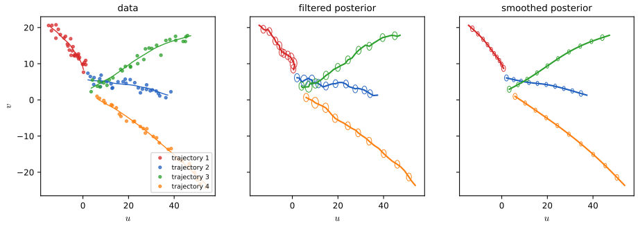
fig_29_26. Download: PDF · SVGData association. In general there are \(M\) detections per step, possibly \(M<N\) (missed detections) or \(M>N\) (clutter), and one must decide which detection came from which object (Figure 29.27 adds a discrete association variable \(m_t\) to the model, which makes exact inference exponential as in Section 29.9.2). The nearest-neighbour approximation builds an \(N\times M\) weight matrix \(W_{im}\) measuring compatibility of object \(i\) and detection \(m\) (typically a Gaussian log density of \(\vy^m\) under object \(i\)'s predicted observation), pads it to a square matrix with dummy objects (for false alarms) and dummy detections (for missed ones), and solves the maximum-weight bipartite matching with the Hungarian algorithm in \(O(\max(N,M)^3)\). Objects matched to a dummy detection get no measurement update, only their predicted state. Belief propagation on the assignment graph (SPADA, with cost \(O(NM)\) per iteration and convergence in a finite number of steps) sums over assignments instead of fixing one and outperforms joint probabilistic data association; SMC is another route. With an unknown number of targets the model is an open-world one, and a common heuristic starts a track for any detection that no current track explains and drops tracks that are undetected for a while (Figure 29.28); random finite sets give a principled treatment.
Filling the gap 29.13: nearest-neighbour data association is a linear assignment problem p. 1052
The book states that the maximum-weight bipartite matching can be found by the Hungarian algorithm. Here is why the MAP assignment is exactly such a matching, under independent measurements.
Derivation
Let each object \(i\) have predicted observation law \(\N(\hat\vy_i,\mS_i)\) and let each detection that is not assigned to an object be clutter with density \(\lambda_c(\vy)\). An assignment is an injective partial map \(\sigma\) from detections to objects; with independent measurements and each object producing at most one detection, \[ \log p(\vy_{1:M}\given\sigma)=\sum_{m:\sigma(m)=i}\log\N(\vy_m\given\hat\vy_i,\mS_i)+\sum_{m\text{ unassigned}}\log\lambda_c(\vy_m) \] plus a term depending only on the number of detections per object (missed-detection probabilities), which we fold into weights. Subtracting the constant \(\sum_m\log\lambda_c(\vy_m)\) leaves \(\sum_{(m,i)\in\sigma}w_{im}\) with \[ w_{im}=\log\N(\vy_m\given\hat\vy_i,\mS_i)-\log\lambda_c(\vy_m)+\log\frac{p_D}{1-p_D} \], where \(p_D\) is the detection probability. Maximising a sum of weights over injective partial maps is a maximum-weight bipartite matching; adding dummy rows and columns with weight 0 makes it a square linear assignment problem, which the Hungarian (Kuhn–Munkres) algorithm solves in cubic time. The code checks that scipy.optimize.linear_sum_assignment reaches the brute-force optimum over all 120 permutations of a random \(5\times5\) weight matrix. ∎
29.10 Nonlinear SSMs
pp. 1053–1054, (29.121)–(29.124) A nonlinear dynamical system has \(\vz_t=f(\vz_{t-1},\vu_t)+\mathbf q_t\), \(\mathbf q_t\sim\N(\mathbf0,\mQ_t)\), \(\vy_t=h(\vz_t,\vu_t)+\mathbf r_t\), \(\mathbf r_t\sim\N(\mathbf0,\mR_t)\) (29.121)–(29.124), the model of Section 8.1.4.
29.10.1 Example: object tracking and state estimation
p. 1054, (29.125), Figure 29.29 Here the motion is linear (Section 29.7.1) and the observation is the bearing to the target from a sensor at \((s_x,s_y)\), \(y_t=\tan^{-1}\!\big((v_t-s_y)/(u_t-s_x)\big)+r_t\) (29.125). The nonlinearity rules out the Kalman filter; the EKF, UKF and other Gaussian filters of Chapter 8 apply. (The figure is a diagram; the EKF with a nonlinear motion model is the subject of Section 8.3.2.)
29.10.2 Posterior inference
p. 1055 Use the extended Kalman filter (Section 8.3.2), the unscented Kalman filter (Section 8.4.2), or the other approximations of Chapter 8 or particle filters (Chapter 13).
29.11 Non-Gaussian SSMs
p. 1055, (29.126)–(29.127) Allow non-Gaussian noise with linear or nonlinear mean functions: \(p(\vz_t\given\vz_{t-1},\vu_t)=p(\vz_t\given f(\vz_{t-1},\vu_t))\), \(p(\vy_t\given\vz_t,\vu_t)=p(\vy_t\given h(\vz_t,\vu_t))\).
29.11.1 Example: spike train modeling
pp. 1055–1056, (29.128), Figures 29.30–29.31 An exponential-family SSM common in neuroscience has linear-Gaussian dynamics and a Poisson likelihood for \(D\) spike counts,
\[ p(\vy_t\given\vz_t)=\prod_{d=1}^D\mathrm{Poi}\big(y_{td}\given\exp(\vw_d^\T\vz_t)\big). \tag{29.128} \]The book fits the model by EM with a Laplace approximation in the E step and the Kalman smoother in the M step; Figure 29.30 gives samples and Figure 29.31 compares the true and the estimated dynamics matrix and latent trajectory. Our model: \(N_z=2\), \(\mathbf A=0.97\,\mathbf R(0.35)\) (a damped rotation), \(\mQ=0.05\mI\), \(D=5\) random loadings, \(T=400\), fitted from a poor start \(\mathbf A=0.9\mI\).
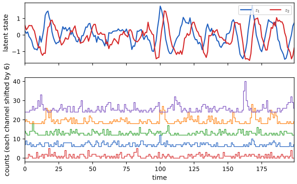
fig_29_30. Download: PDF · SVGFilling the gap 29.14: the Laplace E step for the Poisson LDS and the M step for the loadings p. 1056
"EM with a Laplace approximation" hides three claims: the posterior is log-concave (so the mode is unique and Newton converges), its Hessian is block tridiagonal, and the expected Poisson log-likelihood has a closed form through the Gaussian moment generating function.
Derivation
Log-concavity. The log joint over \(\vz_{1:T}\) is \[ -\tfrac12(\vz_1-\mathbf m_1)^\T\mathbf V_1^{-1}(\vz_1-\mathbf m_1)-\tfrac12\sum_{t\ge2}(\vz_t-\mathbf A\vz_{t-1})^\T\mQ^{-1}(\vz_t-\mathbf A\vz_{t-1})+\sum_{t,d}\big(y_{td}\vw_d^\T\vz_t-e^{\vw_d^\T\vz_t}\big) \]. The first two terms are concave quadratics; each Poisson term is linear minus a convex function, hence concave. So the posterior is log-concave and has a unique mode. Hessian. The negative Hessian is block tridiagonal: diagonal blocks \[ \mQ^{-1}+\mathbf A^\T\mQ^{-1}\mathbf A+\sum_d e^{\vw_d^\T\vz_t}\vw_d\vw_d^\T \] (with \(\mathbf V_1^{-1}\) instead of \(\mQ^{-1}\) at \(t=1\), and no \(\mathbf A^\T\mQ^{-1}\mathbf A\) at \(t=T\)) and off-diagonal blocks \(-\mQ^{-1}\mathbf A\) and its transpose. Newton's method \(\vz\leftarrow\vz+\bm\Lambda^{-1}\mathbf g\) (with backtracking) converges to the mode \(\vz^*\), and the Laplace approximation is \(\N(\vz^*,\bm\Lambda^{-1})\); the diagonal blocks of \(\bm\Lambda^{-1}\) are the marginal covariances and the sub-diagonal blocks the lag-one covariances (the same output as the Kalman smoother, which exploits the block structure to cost \(O(TN_z^3)\); our code inverts the dense matrix for clarity). M step. With the Gaussian approximation \(\vz_t\sim\N(\vm_t,\mathbf S_t)\), the update of \((\mathbf A,\mathbf Q,\mathbf m_1,\mathbf V_1)\) is the regression lemma of Filling the gap 29.10. For the loadings, \(\E[e^{\vw^\T\vz_t}]=\exp(\vw^\T\vm_t+\tfrac12\vw^\T\mathbf S_t\vw)\) (Gaussian MGF), so \(\vw_d\) maximises the concave function \[ \sum_t[y_{td}\vw^\T\vm_t-\exp(\vw^\T\vm_t+\tfrac12\vw^\T\mathbf S_t\vw)] \], solved by a few Newton steps. Caveat. Because the E step is approximate, the likelihood is not guaranteed to increase at every iteration. Identifiability. For any invertible \(\mathbf G\), replacing \(\vz\to\mathbf G\vz\), \(\mathbf A\to\mathbf G\mathbf A\mathbf G^{-1}\), \(\mQ\to\mathbf G\mQ\mathbf G^\T\), \(\vw_d\to\mathbf G^{-\T}\vw_d\) leaves the data law unchanged, so Figure 29.31 compares the two models after mapping the estimated latent space onto the true one by least squares. In our run the eigenvalues of the estimated \(\mathbf A\) are \(0.892\pm0.318i\) against \(0.911\pm0.333i\) for the true one, and the aligned latent trajectory explains 85% of the variance of the true one. ∎
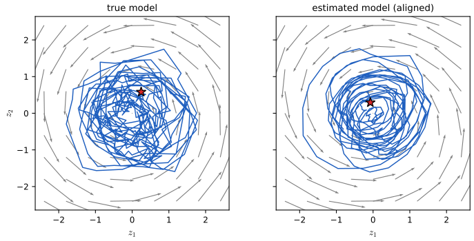
fig_29_31. Download: PDF · SVG29.11.2 Example: stochastic volatility models
pp. 1056–1057, (29.129)–(29.134) For log-returns \(y_t=\log(p_t/p_{t-1})\) the stochastic volatility model is
\[ y_t=\vu_t^\T\bm\beta+\exp(z_t/2)\,r_t,\qquad z_t=\mu+\rho(z_{t-1}-\mu)+\sigma q_t,\qquad r_t,q_t\sim\N(0,1), \tag{29.129–29.132} \]with \(|\rho|<1\) for stationarity; the log-variance \(z_t\) follows an AR(1), and a Student likelihood gives heavier tails. For an AR(2) volatility, stack the last two values: \[ (z_t-\mu,z_{t-1}-\mu)^\T=\begin{pmatrix}\rho_1&\rho_2\\1&0\end{pmatrix}(z_{t-1}-\mu,z_{t-2}-\mu)^\T+(q_t,0)^\T \] (29.133), i.e. \(z_t=\mu+\rho_1(z_{t-1}-\mu)+\rho_2(z_{t-2}-\mu)+q_t\) (29.134), the standard way to write any higher-order autoregression as a first-order state-space model.
29.11.3 Posterior inference
p. 1057 Use the Gaussian approximations of Chapter 8 or the sequential Monte Carlo methods of Chapter 13.
29.12 Structural time series models
pp. 1057–1069 Time series forecasting means computing \(p(\vy_{t+h}\given\vy_{1:t})\) (optionally given known future inputs). Structural time series (STS) models do this with linear-Gaussian SSMs. Many classical methods (ARMA, exponential smoothing) are special cases, and the STS framework extends to nonlinear, non-Gaussian and hierarchical models.
29.12.1 Introduction
pp. 1057–1058, (29.135)–(29.139) Represent the series as a sum of \(C\) components plus noise, \(f(t)=f_1(t)+\dots+f_C(t)+\epsilon_t\), \(\epsilon_t\sim\N(0,\sigma^2)\) (29.135), each \(f_c\) a linear-Gaussian SSM (a dynamic linear model, DLM). Linear systems add, so the whole is one LG-SSM with block-structured \(\mF,\mQ\):
\[ p(\vz_t\given\vz_{t-1},\bm\theta)=\N(\vz_t\given\mF\vz_{t-1},\mQ),\qquad p(y_t\given\vz_t,\bm\theta)=\N(y_t\given\mH\vz_t+\bm\beta^\T\vu_t,\sigma_y^2). \tag{29.136–29.137} \]\(\mF\) and \(\mH\) are fixed sparse matrices set by the components; the only parameters are the variances in \(\mQ\), \(\sigma_y^2\) and the regression coefficients \(\bm\beta\). (Vector-valued observations: (29.138)–(29.139).)
29.12.2 Structural building blocks
29.12.2.1 Local level model
p. 1058, (29.140)–(29.141) Observations scatter around a latent mean that follows a random walk, \(y_t=\mu_t+\epsilon_{y,t}\), \(\mu_t=\mu_{t-1}+\epsilon_{\mu,t}\) with variances \(\sigma_y^2\), \(\sigma_\mu^2\). With \(\mu_1\sim\N(0,\sigma_\mu^2)\) we get \(\mu_t\sim\N(0,t\sigma_\mu^2)\), whose variance grows without bound; an AR(1) version \(\mu_t=\rho\mu_{t-1}+\epsilon_{\mu,t}\), \(|\rho|<1\), has the stationary variance \(\sigma_\mu^2/(1-\rho^2)\) and the uncertainty levels off.
Filling the gap 29.15: the local level filter is exponential smoothing, with a closed-form gain p. 1058, (29.140)–(29.141)
The steady state of the local-level Kalman filter is solved in Problem 8.1 of Chapter 8; here are the consequences that matter for forecasting.
Derivation
Growth of variance. By independence of the increments, \(\var\mu_t=\var\mu_1+(t-1)\sigma_\mu^2=t\sigma_\mu^2\). For the AR(1) version \(v_t=\rho^2v_{t-1}+\sigma_\mu^2\), whose fixed point is \(\sigma_\mu^2/(1-\rho^2)\). Steady state. Let \(P\) be the predicted variance. The filtered variance is \(P\sigma_y^2/(P+\sigma_y^2)\) and the next predicted variance adds \(\sigma_\mu^2\): at a fixed point \(P^2-\sigma_\mu^2P-\sigma_\mu^2\sigma_y^2=0\), so \(P=\tfrac12(\sigma_\mu^2+\sqrt{\sigma_\mu^4+4\sigma_\mu^2\sigma_y^2})\). With the signal-to-noise ratio \(q=\sigma_\mu^2/\sigma_y^2\), \(P/\sigma_y^2=\tfrac12(q+\sqrt{q^2+4q})\) and the gain is \(k=P/(P+\sigma_y^2)\) (for \(q=1\): \(k=0.618\)). Exponential smoothing. The filtered mean obeys \(\hat\mu_t=\hat\mu_{t-1}+k(y_t-\hat\mu_{t-1})=(1-k)\hat\mu_{t-1}+ky_t\), the weight on \(y_{t-j}\) being \(k(1-k)^j\): simple exponential smoothing with smoothing constant \(\alpha=k\) (equivalently an ARIMA(0,1,1) model), and the effective window is \(1/k\) observations. Forecast. The \(h\)-step forecast mean is the last filtered mean (the level is a martingale) and the variance is \(\Sigma_{t|t}+h\sigma_\mu^2+\sigma_y^2\). The code confirms the closed-form steady state, the equality of the filter with exponential smoothing at gain \(k\), and the forecast variance formula to \(10^{-8}\). The value of \(\sigma_\mu\) thus sets how fast old data are forgotten; this is the trade-off visible in the first two presets of the forecasting demonstration. ∎
29.12.2.2 Local linear trend model
pp. 1058–1059, (29.142)–(29.146) To allow a local trend, let the level move by the slope, \(\mu_t=\mu_{t-1}+\delta_{t-1}+\epsilon_{\mu,t}\), and let the slope follow a random walk, \(\delta_t=\delta_{t-1}+\epsilon_{\delta,t}\) (29.142)–(29.143), which in state form (state \((\mu_t,\delta_t)\)) is
\[ \begin{pmatrix}\mu_t\\\delta_t\end{pmatrix}=\begin{pmatrix}1&1\\0&1\end{pmatrix}\begin{pmatrix}\mu_{t-1}\\\delta_{t-1}\end{pmatrix}+\begin{pmatrix}\epsilon_{\mu,t}\\\epsilon_{\delta,t}\end{pmatrix},\qquad y_t=(1\ \ 0)\begin{pmatrix}\mu_t\\\delta_t\end{pmatrix}+\epsilon_{y,t}. \tag{29.144–29.145} \]An AR(1) slope \(\delta_t=D+\rho(\delta_{t-1}-D)+\epsilon_{\delta,t}\) (29.146) reverts to a long-run slope \(D\): the semi-local linear trend, better for long horizons.
29.12.2.3 Adding covariates
p. 1059, (29.147), Figure 29.32a A linear regression on inputs, \(y_t=\mu_t+\bm\beta^\T\vu_t+\epsilon_{y,t}\) (29.147). To forecast one needs the future inputs; a simple choice is \(\vu_{t+h}=\vu_t\).
29.12.2.4 Modelling seasonality
p. 1060, (29.148), Figure 29.32b Offsets \(s_t\) that sum to zero (on average) over a cycle of \(S\) steps, \(s_t=-\sum_{k=1}^{S-1}s_{t-k}+\epsilon_{s,t}\) (29.148); stacking the last \(S-1\) values makes it first order.
29.12.2.5 Adding it all up
p. 1060, (29.149) The components combine in one state, for instance for \(S=4\) with state \((s_t,s_{t-1},s_{t-2},\mu_t,\delta_t)\), a block-diagonal \(\mF\) (the seasonal block has first row \((-1,-1,-1)\) and a shifted identity below) and noise covariance \(\mathrm{diag}(\sigma_s^2,0,0,\sigma_\mu^2,\sigma_\delta^2)\). The observation matrix adds \(s_t\) and \(\mu_t\). The code builds this for any period (sts_matrices).
Filling the gap 29.16: how forecast uncertainty grows, and the seasonal block pp. 1058–1060, (29.142)–(29.150)
The book says forecasts are obtained by rolling the state forward and predicting; here is what that gives for the local linear trend (variance growing cubically) and why the dummy-variable seasonal block works.
Derivation
Local linear trend. Unrolling (29.142)–(29.143) from time \(t\): \(\delta_{t+k}=\delta_t+\sum_{j=1}^k\epsilon_{\delta,t+j}\) and \[ \mu_{t+h}=\mu_t+h\delta_t+\sum_{k=1}^h\epsilon_{\mu,t+k}+\sum_{k=1}^{h-1}(h-k)\epsilon_{\delta,t+k} \]. With the filtered covariance \(\bSig_{t|t}\) of \((\mu_t,\delta_t)\),
\[ \var(y_{t+h}\given\vy_{1:t})=\Sigma_{\mu\mu}+2h\Sigma_{\mu\delta}+h^2\Sigma_{\delta\delta}+h\,\sigma_\mu^2+\sigma_\delta^2\sum_{k=1}^{h-1}(h-k)^2+\sigma_y^2,\qquad \sum_{k=1}^{h-1}(h-k)^2=\frac{(h-1)h(2h-1)}{6}. \]The slope noise contributes a cubic term, so the forecast band opens like \(h^{3/2}\) in standard deviation; this is why a slope noise of 0.05 (preset 3 of the forecasting demonstration) (with level noise 0.6) produces a band of sd 44 ppm after ten years. The formula equals the Kalman prediction recursion to \(10^{-10}\) (confirmed). Seasonal block. The state \((s_t,\dots,s_{t-S+2})\) evolves by \(s_t=-\sum_{k=1}^{S-1}s_{t-k}\) without noise, which is equivalent to \(\sum_{k=0}^{S-1}s_{t-k}=0\) for all \(t\); subtracting this relation at \(t\) and \(t-1\) gives \(s_t=s_{t-S}\), so the pattern repeats exactly with period \(S\) and sums to zero over a cycle (confirmed). With \(\sigma_s>0\) the pattern can drift while the sum constraint is only kept on average. The \(S-1\) dimensional state is the minimum for a zero-sum period-\(S\) pattern. ∎
29.12.3 Model fitting
p. 1060, (29.151) With \(\mF,\mH\) fixed by the components, the parameters are the variances and \(\bm\beta\): fit by maximum likelihood (Section 29.8) or Bayesian inference; the Bayesian version is Bayesian structural time series (BSTS), usually with the conjugate prior (29.151) \(p(\bm\theta)=\mathrm{MNIW}(\mR,\mathbf D)\,\mathrm{IW}(\mQ)\) and spike-and-slab priors on \(\bm\beta\) when there are many covariates.
29.12.4 Forecasting
p. 1061, (29.150) Run the Kalman filter on the data, then roll forward in latent space: \[ p(y_{t+1}\given\vy_{1:t})=\int p(y_{t+1}\given\vz_{t+1})p(\vz_{t+1}\given\vz_t)p(\vz_t\given\vy_{1:t})\,\d\vz_t \], a Gaussian given by the prediction step of Section 8.2.2; repeating \(h\) times gives \(p(y_{t+h}\given\vy_{1:t})\). With uncertain parameters, average forecasts over posterior samples.
29.12.5 Examples
29.12.5.1 Example: forecasting CO2 levels from Mauna Loa
p. 1061, Figure 29.33 Local linear trend plus seasonal with \(S=12\), fitted to all but the last 10 years. The book uses the 1966–2019 record and fits by variational Bayes (\(\sigma_y=0.169\), \(\sigma_\mu=0.159\), \(\sigma_\delta=0.009\), \(\sigma_s=0.038\)). That record is not bundled with the tools used here, so we use the weekly 1958–2001 record shipped with statsmodels, averaged by month (526 months with five gaps, treated as missing), and fit by maximum likelihood with a vague prior on the initial state: \(\hat\sigma_y=0.168\), \(\hat\sigma_\mu=0.214\), \(\hat\sigma_\delta=0.002\) and \(\hat\sigma_s\approx0\) (a nearly fixed annual pattern). The first two agree with the book's to within 35%. The ten-year forecast has an RMSE of 1.04 ppm. The same series is modelled by a Gaussian process in Section 18.8.1.
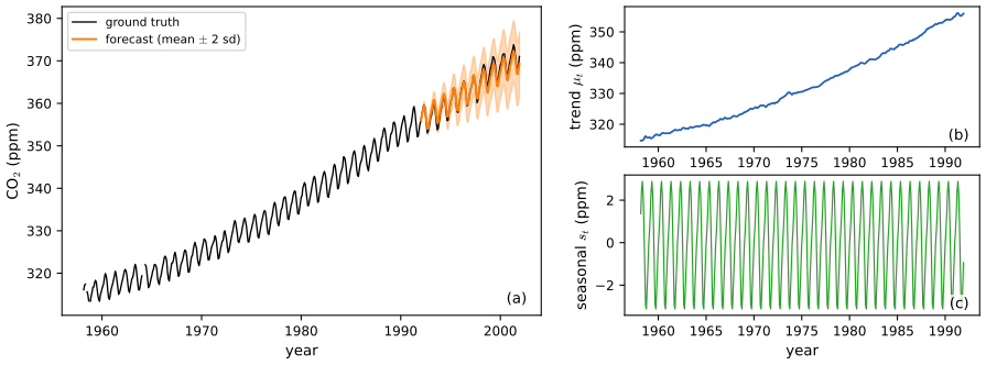
fig_29_33. Download: PDF · SVG29.12.5.2 Example: forecasting (real-valued) electricity usage
pp. 1062–1063, Figures 29.34–29.36 Hourly demand in Victoria, Australia (January and February 2014) is forecast from temperature using four components (an hourly effect of period 24, a daily effect of period 7 with 24 steps per season, a regression on temperature and an autoregressive term on the observations), fitted by variational inference; the regression on temperature is the most important effect, and the autoregressive component is the most uncertain because it absorbs all residual structure. Figures 29.34 and 29.35 need the 2014 demand and temperature series, which are not available here, and are not reproduced.
Anomaly detection (Figure 29.36) needs only the one-step-ahead predictive distribution \(p(y_t\given\vy_{1:t-1},\vu_{1:t})=\N(\hat y_t,S_t)\) that the Kalman filter computes anyway: flag \(t\) when the z-score \((y_t-\hat y_t)/\sqrt{S_t}\) is large (the book uses \(>3\)). Under the true model the z-scores are exactly iid \(\N(0,1)\) (they are the standardised innovations), so the false-alarm rate is about 0.27% per step for \(|z|>3\); in a long simulation from the model their mean was 0.013 and their variance 1.009. Figure x29.a demonstrates the idea on a simulated hourly-like series (local level plus a period-24 pattern) with five injected anomalies.
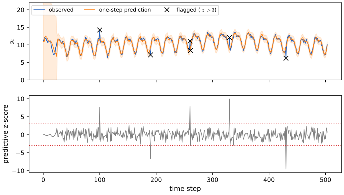
fig_x29_a. Download: PDF · SVG29.12.5.3 Example: forecasting (integer valued) sales
pp. 1062–1064, Figure 29.37 For counts \(y_t\in\{0,1,\dots\}\) use a Poisson likelihood \(y_t\sim\mathrm{Poi}(g(d_t))\) with instantaneous latent demand \(d_t=z_t+\vu_t^\T\vw\), transfer function \(g(d)=e^d\) or \(\log(1+e^d)\), covariates \(\vu_t\) for seasonal indicators, and a random-walk \(z_t=z_{t-1}+\alpha\N(0,1)\) for serial correlation. Zero counts may reflect stock-outs rather than zero demand; a zero-inflated Poisson \(p_0\mathbb I(y_t=0)+(1-p_0)\mathrm{Poi}(y_t\given e^{d_t})\) or a negative binomial helps, but is not log-concave at \(d_t=0\) (so a Laplace approximation can land on a saddle); a multi-stage log-concave likelihood fixes that. The figure is taken from a paper and is not redrawn.
29.12.5.4 Example: hierarchical SSM for electoral panel data
pp. 1064–1065, (29.152)–(29.155), Figure 29.38 For state \(j\) let \(N^j_t\) voters of whom \(y^j_t\) vote Democrat: \(y^j_t\sim\mathrm{Bin}(\pi^j_t,N^j_t)\), \(\pi^j_t=\sigma[(\vz^0_t)^\T\vu^0_t+(\vz^j_t)^\T\vu^j_t]\), with a national random walk \(\vz^0_t=\vz^0_{t-1}+\N(\mathbf0,\sigma^2\mI)\) and state-level random effects \(\vz^j_t=\vz^j_{t-1}+\N(\mathbf0,\tau^2\mI)\) (29.152)–(29.155). The hierarchy shares information across states and time.
29.12.6 Causal impact of a time series intervention
pp. 1065–1068, (29.156)–(29.161), Figures 29.39–29.41 Suppose an intervention (an ad campaign) occurs after time \(n\) and outcomes \(y_{1:n}\) (before) and \(y_{n+1:m}\) (after) are observed. The causal effect is the difference between the observed outcome and what would have happened without intervention, a counterfactual. An STS is a structural causal model (arrows follow time), so the counterfactual can be computed by the twin-network recipe: infer the exogenous noise and state before the intervention, then roll a copy of the model forward without it. The target is
\[ p(\tilde\vy_{n+1:m}\given\vy_{1:n},\vx_{1:m})=\int p(\tilde\vy_{n+1:m}\given\tilde\vz_{n+1:m},\vx_{n+1:m},\bm\theta)\,p(\tilde\vz_{n+1:m}\given\vz_n,\bm\theta)\,p(\vz_n,\bm\theta\given\vx_{1:n},\vy_{1:n})\,\d\bm\theta\,\d\vz_n\,\d\tilde\vz_{n+1:m} \tag{29.156–29.158} \](with covariates \(\vx_t\) assumed unaffected). The Kalman filter gives \(p(\vz_n\given\cdot,\bm\theta)\) and MCMC or VI gives \(p(\bm\theta\given\cdot)\). Posterior samples give the effect per step \(\tau_t=y_t-\tilde y_t\) and the cumulative effect \(\sum_{s>n}\tau_s\). Three assumptions: predictability (the model can predict the outcome; test by backcasting), unaffectedness (covariates are not changed by the intervention) and stability (the pre-period model would have continued; test by shifting the intervention date earlier). A linear combination of covariates plays the role of a synthetic control, without the convexity restriction, and spike-and-slab or horseshoe priors choose among many donors.
Filling the gap 29.17: the counterfactual forecast is a joint Gaussian, so the cumulative impact needs its full covariance pp. 1066–1067, (29.156)–(29.158)
For fixed parameters the integral (29.156) is Gaussian and available in closed form. What the book does not say is that the forecasts of different days are strongly correlated through the shared state, so the uncertainty of the cumulative effect cannot be read off the pointwise uncertainties.
Derivation
Fix \(\bm\theta\). The state follows \(\vz_{s+1}=\mF\vz_s+\mathbf q_s\) with filtered law \(\N(\vm_n,\mathbf P_n)\) at time \(n\); put \(\mathbf P_{n+k|n}=\mF\mathbf P_{n+k-1|n}\mF^\T+\mQ\), \(\vm_{n+k|n}=\mF^k\vm_n\). For \(i\ge j\), \(\vz_{n+i}=\mF^{i-j}\vz_{n+j}+\)(noise independent of \(\vz_{n+j}\)), so \(\mathrm{Cov}(\vz_{n+i},\vz_{n+j})=\mF^{i-j}\mathbf P_{n+j|n}\). With the observation \(\tilde y_{n+i}=\mH_{n+i}\vz_{n+i}+\epsilon_i\) (time-varying \(\mH\) because the covariates enter through it),
\[ \mathrm{Cov}(\tilde y_{n+i},\tilde y_{n+j})=\mH_{n+i}\mF^{i-j}\mathbf P_{n+j|n}\mH_{n+j}^\T+\delta_{ij}\sigma_y^2\quad(i\ge j). \]The vector \(\tilde\vy_{n+1:m}\) is Gaussian with this covariance \(\mathbf C\) and mean \(\mH_{n+i}\vm_{n+i|n}\). Given the observed \(\vy\), \(\tau_t=y_t-\tilde y_t\) has the same covariance, and the cumulative effect \(\sum_{s=n+1}^t\tau_s\) has mean \(\sum(y_s-\E\tilde y_s)\) and variance \(\mathbf1^\T\mathbf C_{(t)}\mathbf1\), the sum of all entries of the leading block, not just the diagonal. Positive off-diagonal entries (a common level error persists) make this far larger than \(\sum_s\mathrm{Var}(\tilde y_s)\). For variances \(\sigma_y=0.5,\sigma_\mu=0.15,\sigma_\delta=0.02\) in our simulated example the closed-form sd of the 30-day cumulative forecast is 44.5, which agrees with a Monte Carlo simulation of 20,000 paths (44.6), while the independent-sum value is only 9.9 (all at a fixed parameter vector). The parameters themselves are fitted (here by maximum likelihood on the pre-period), not integrated out as in (29.156), so our intervals understate the parameter uncertainty that a full BSTS would add. ∎
Example (pp. 1068, Figure 29.41). Following the book, \(x_t\) is an AR(1) series (\(\rho=0.9\)), \(y_t=1.2x_t+\epsilon_t\) with \(\sigma_\epsilon=0.5\), and at \(t=70\) (of 100) we add 10 to every later \(y_t\). The model is a local level with slope (29.159)–(29.161) and a regression coefficient \(\beta\) carried as a static state. Fitting the three variances on the first 70 points by maximum likelihood, the counterfactual forecast follows the AR trend of \(x\); the pointwise impact has mean \(10.08\) over the post-period and the cumulative effect after 30 days is \(302.3\pm1.96\times5.9\), containing the true 300.
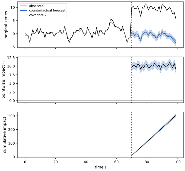
fig_29_41. Download: PDF · SVG29.12.7 Prophet
p. 1069, (29.162)–(29.163) Prophet is a generalised additive regression \(y(t)=g(t)+s(t)+h(t)+\vw^\T\vx(t)+\epsilon_t\) (29.162) with a piecewise-linear trend \(g(t)=(k+\mathbf a(t)^\T\bm\delta)t+(m+\mathbf a(t)^\T\bm\gamma)\), \(a_j(t)=\mathbb I(t\ge s_j)\), changepoints \(s_j\) on a regular grid, Laplace prior \(\delta_j\sim\mathrm{Laplace}(\tau)\) (so most slope changes vanish at the MAP) and \(\gamma_j=-s_j\delta_j\) to keep \(g\) continuous (29.163), a Fourier-basis seasonal term and sparse holiday effects. It regresses on time, not on past values, so it is not autoregressive.
29.12.8 Neural forecasting methods
pp. 1069–1070 With much data (a very long series, or many related ones) flexible networks become competitive. Examples: ES-RNN (exponential smoothing for the local series plus an RNN trained across series, winner of the M4 competition), DeepSSM (an RNN predicts the time-varying parameters of a linear SSM, trained through the Kalman-filter likelihood \(\sum_nL_n\)), Deep Factors, DeepGLO, N-BEATS (residual network predicting basis-function weights), DeepAR (an RNN fitted to many series with a count likelihood, or mixtures), quantile regression with the pinball loss, SQF-RNN trained on the CRPS \(\int_0^12\ell_\alpha(y,F^{-1}(\alpha))\,\d\alpha\), copulas for several outputs and MQ-CNN. For deterministic forecasts the CRPS reduces to the absolute error.
29.13 Deep SSMs
pp. 1070–1075 Dropping linearity and Gaussianity, let the dynamics and observation models be deep networks (a dynamical variational autoencoder). The observations are written \(\vx_t\) as in the VAE literature (Chapter 21).
29.13.1 Deep Markov models
pp. 1071–1072, (29.164)–(29.171), Figure 29.42 A deep Markov model (DMM, stochastic RNN) uses neural networks for \(p(\vz_t\given\vz_{t-1})\) and/or \(p(\vx_t\given\vz_t)\) and is fitted by SVI. The exact posterior factorises with first-order structure,
\[ p(\vz_{1:T}\given\vx_{1:T})=\prod_{t=1}^Tp(\vz_t\given\vz_{t-1},\vx_{1:T})=\prod_{t=1}^Tp(\vz_t\given\vz_{t-1},\vx_{t:T}), \tag{29.164} \]so an inference network may take the form \(q(\vz_{1:T}\given\vx_{1:T})=\prod_tq(\vz_t\given\vz_{t-1},\vx_{t:T})\) (29.165) with the future summarised by a backwards RNN (29.166), or the simpler causal \(\prod_tq(\vz_t\given\vx_{1:t})\) which can run online. For a fully factorised \(q\), the ELBO is
\[ \log p(\vx_{1:T})\ \ge\ \sum_{t=1}^T\E_{q(\vz_t)}[\log p(\vx_t\given\vz_t)]-\E_{q(\vz_{t-1})}\big[\KL\big(q(\vz_t)\,\|\,p(\vz_t\given\vz_{t-1})\big)\big]. \tag{29.171} \]Filling the gap 29.18: the first-order posterior factorisation and the ELBO (29.171) pp. 1071–1072, (29.164)–(29.171)
(29.164) is quoted from the DMM paper. It rests on one conditional independence, and the ELBO is the chain-rule decomposition with a factorised \(q\).
Derivation
(29.164). The model factorises as \[ p(\vz_{1:T},\vx_{1:T})=g(\vz_{1:t-1},\vx_{1:t-1})\,p(\vz_t\given\vz_{t-1})\,h(\vz_{t:T},\vx_{t:T}) \], where \(g\) collects \(p(\vz_1)\), the transitions up to \(t-1\) and the emissions up to \(t-1\), and \(h\) the emission at \(t\), and everything after \(t\) (transitions from \(t+1\), emissions from \(t\)). Fix \(\vz_{t-1}\) and the whole data \(\vx_{1:T}\) and integrate out \(\vz_{1:t-2}\) and \(\vz_{t+1:T}\): \[ p(\vz_t,\vz_{t-1},\vx_{1:T})=\tilde g(\vz_{t-1},\vx_{1:t-1})\,p(\vz_t\given\vz_{t-1})\,\tilde h(\vz_t,\vx_{t:T}) \]. As a function of \(\vz_t\) this is proportional to \(p(\vz_t\given\vz_{t-1})\tilde h(\vz_t,\vx_{t:T})\); the factor \(\tilde g\), the only place \(\vx_{1:t-1}\) appears, does not involve \(\vz_t\) and cancels on normalising. So \(p(\vz_t\given\vz_{t-1},\vx_{1:T})\) does not depend on \(\vx_{1:t-1}\), i.e. \(\vz_t\perp\vx_{1:t-1}\given\vz_{t-1},\vx_{t:T}\). The same argument with \(\vz_{1:t-2}\) shows that \(\vz_t\) is conditionally independent of \(\vz_{1:t-2}\) given \(\vz_{t-1},\vx_{1:T}\), so the chain rule \(p(\vz_{1:T}\given\vx)=\prod_tp(\vz_t\given\vz_{1:t-1},\vx_{1:T})\) reduces to (29.164). We confirm it by enumeration on a small discrete HMM. ELBO. For any \(q\), \[ \log p(\vx_{1:T})\ge\E_q[\log p(\vx_{1:T},\vz_{1:T})-\log q(\vz_{1:T})] \] (Jensen, as in (29.167)–(29.170)). With \(q=\prod_tq(\vz_t)\) the expectation splits into \[ \sum_t\E_{q(\vz_t)}\log p(\vx_t\given\vz_t)+\sum_t\E_{q(\vz_t)q(\vz_{t-1})}\log p(\vz_t\given\vz_{t-1})-\sum_t\E_{q(\vz_t)}\log q(\vz_t) \], and \[ \E_{q(\vz_t)q(\vz_{t-1})}[\log p(\vz_t\given\vz_{t-1})-\log q(\vz_t)]=-\E_{q(\vz_{t-1})}\KL(q(\vz_t)\|p(\vz_t\given\vz_{t-1})) \] exactly, giving (29.171) (for \(t=1\) the KL is to \(p(\vz_1)\)). In a Gaussian linear model with an arbitrary factorised Gaussian \(q\) the closed form (KL of Gaussians averaged over \(q(\vz_{t-1})\)) matches a 400,000-sample Monte Carlo estimate to 0.004 and lies below the Kalman log-evidence, as it must. With Gaussians and the reparametrisation trick the bound has low-variance gradients, and the KL terms are analytic. ∎
29.13.2 Recurrent SSM
p. 1072, Figure 29.43 To capture long-range dependence, add deterministic hidden states \(\vh_t=f(\vh_{t-1},\vz_t)\) summarising \(\vz_{1:t}\): the observation model becomes \(p(\vx_t\given\vh_t)\) (Figure 29.43a) and, in the recurrent SSM (RSSM), the prior too, \(p(\vz_t\given\vh_{t-1})\) (Figure 29.43b). The inference network uses a forwards RNN to compute \(q(\vz_t\given\vx_{1:t})\).
29.13.3 Improving multistep predictions
pp. 1073–1074, (29.172)–(29.175), Figure 29.44 In the standard bound the dynamics \(p(\vz_t\given\vz_{t-1})\) is only ever compared with the one-step posterior \(q(\vz_t)\), which can hurt long-horizon prediction. Observation overshooting adds reconstruction losses for observations predicted \(d\) steps ahead from the latent rollout. Latent overshooting (Hafner et al.) does this in latent space: with the \(d\)-step prior \(p(\vz_t\given\vz_{t-d})\) (obtained by composing the transition and integrating out the intermediate states),
\[ \log p_d(\vx_{1:T})\triangleq\log\int\prod_{t=1}^Tp(\vz_t\given\vz_{t-d})p(\vx_t\given\vz_t)\,\d\vz_{1:T}\ \ge\ \sum_{t=1}^T\E_{q(\vz_t)}\log p(\vx_t\given\vz_t)-\E_{p(\vz_{t-1}\given\vz_{t-d})q(\vz_{t-d})}\KL\big(q(\vz_t)\|p(\vz_t\given\vz_{t-1})\big), \tag{29.172–29.173} \]and one averages over \(d=1,\dots,D\), in practice only the KL terms with weights \(\beta_d\) (29.174)–(29.175).
Filling the gap 29.19: the overshooting KL is an upper bound on the exact \(d\)-step KL, so (29.173) is a looser bound p. 1074, (29.172)–(29.173)
The book states the inequality (29.173). It is true, but the penalty it uses is not the one the exact derivation gives.
Derivation
Repeat the ELBO argument of Filling the gap 29.18 with the \(d\)-step prior: for factorised \(q\), \[ \log p_d(\vx_{1:T})\ge\sum_t\E_{q}\log p(\vx_t\given\vz_t)-\sum_t\E_{q(\vz_{t-d})}\KL(q(\vz_t)\|p(\vz_t\given\vz_{t-d})) \]. In (29.173) the second term is instead \[ \E_{p(\vz_{t-1}\given\vz_{t-d})q(\vz_{t-d})}\KL(q(\vz_t)\|p(\vz_t\given\vz_{t-1})) \], the KL to the one-step prior from a sampled intermediate state. Since \[ p(\vz_t\given\vz_{t-d})=\E_{p(\vz_{t-1}\given\vz_{t-d})}[p(\vz_t\given\vz_{t-1})] \] is a mixture and \(\KL(q\|\cdot)\) is convex in its second argument, Jensen gives \[ \KL(q\|p(\cdot\given\vz_{t-d}))\le\E_{p(\vz_{t-1}\given\vz_{t-d})}\KL(q\|p(\cdot\given\vz_{t-1})) \]. Hence the penalty in (29.173) is at least the exact one, and (29.173) is a valid but looser lower bound (\(\le\) the exact \(d\)-step bound \(\le\log p_d\)). Its advantage is that every term involves only the one-step transition model, which is a neural network that can be sampled and evaluated, whereas the \(d\)-step prior is not available in closed form. For a scalar linear-Gaussian model with \(a=0.9\), \(q=0.3\), \(d=2\), the book's penalty is 1.118 against 0.421 for the exact two-step KL (the numbers depend on \(q(\vz)\); the inequality holds for all of them). ∎
29.13.4 Variational RNNs
pp. 1074–1075, (29.176)–(29.177), Figure 29.45 A variational RNN conditions the latent on all past latents and observations through a deterministic \(\vh_t=f(\vh_{t-1},\vx_{t-1},\vz_t)\): \[ p(\vx_{1:T},\vz_{1:T},\vh_{1:T})=\prod_tp(\vz_t\given\vh_{t-1},\vx_{t-1})\,\mathbb I(\vh_t=f(\vh_{t-1},\vx_{t-1},\vz_t))\,p(\vx_t\given\vh_t) \] (29.176). Marginalising \(\vh\), the prior is \(p(\vz_t\given\vz_{1:t-1},\vx_{1:t-1})\) (a DMM has \(p(\vz_t\given\vz_{t-1})\), an RSSM \(p(\vz_t\given\vz_{1:t-1})\)), and the inference network is \(q(\vz_t\given\vz_{1:t-1},\vx_{1:t})\) (29.177), or with a bidirectional RNN \(q(\vz_t\given\vz_{1:t-1},\vx_{1:T})\) for the smoothed posterior. It is more expressive but slower to forecast with, since rolling out needs generated observations as inputs, so it is less used for model-based RL. Applications include stochastic video generation.
Continuous time SSMs (supplement 29.1)
supplement pp. 219–224, (S29.1)–(S29.32) Many physical systems are continuous in time; observations arrive at discrete times.
Ordinary differential equations (supplement 29.1.1)
For a scalar state with \(\dot z=f(t,z)\), advance from one observation time to the next by integration, \(z_{i+1}=z_i+\int_{t_i}^{t_{i+1}}f(t,z)\,\d t\) (the book's (S29.2) writes the limits as \(t_{i-1}\) to \(t_i\) and the left side as \(z_{i+1}\), which does not match; the interval must be \([t_i,t_{i+1}]\)). The second-order Runge–Kutta (Heun) rule with step \(\Delta\) is
\[ k_1=f(t_i,z_i),\quad k_2=f(t_i+\Delta,z_i+k_1\Delta),\quad z_{i+1}=z_i+\tfrac\Delta2(k_1+k_2), \tag{S29.3–S29.5} \]the step size times the average of the slopes at the two ends (Figure S29.1, a schematic). For vector states with conditionally independent components the integral reduces to scalar ones.
Example: noiseless 1d spring-mass system (supplement 29.1.2)
An object of mass \(m\) on a spring with constant \(c\) and viscous friction \(b\), driven by a force \(u(t)\), obeys \(m\ddot x=u-b\dot x-cx\) (S29.6). With state \(\vz=(x,\dot x)\) and only the position observed, \(\dot{\vz}=\mF\vz+\mathbf Bu\), \(y=\mH\vz\) with \(\mF=\begin{pmatrix}0&1\\-c/m&-b/m\end{pmatrix}\), \(\mathbf B=(0,1/m)^\T\), \(\mH=(1,0)\) (S29.7)–(S29.10). To simulate at times \(t_k=k\Delta\) one discretises with the generalised bilinear transform
\[ \mF_d=(\mI-\alpha\Delta\mF)^{-1}(\mI+(1-\alpha)\Delta\mF),\qquad \mathbf B_d=\Delta(\mI-\alpha\Delta\mF)^{-1}\mathbf B, \tag{S29.11} \]with \(\alpha=0\) Euler's method (S29.12), \(\alpha=1\) backward Euler and \(\alpha=\tfrac12\) the bilinear rule, which preserves stability.
Filling the gap 29.20: Runge–Kutta order 2, and why the bilinear transform keeps systems stable supplement pp. 219–221, (S29.3)–(S29.12)
The supplement states both facts. Each is a two-line computation.
Derivation
RK2 is second order. Taylor-expand the exact flow of \(\dot z=f(z)\) (autonomous for simplicity): \(z(t+\Delta)=z+\Delta f+\tfrac12\Delta^2f'f+O(\Delta^3)\). The Heun step is \[ z+\tfrac\Delta2(f(z)+f(z+\Delta f))=z+\tfrac\Delta2(2f+\Delta f'f+O(\Delta^2))=z+\Delta f+\tfrac12\Delta^2f'f+O(\Delta^3) \], so the local error is \(O(\Delta^3)\) and the global error over a fixed horizon is \(O(\Delta^2)\): halving the step divides the error by 4 (we find ratio 4.10 for \(\dot z=-3z\) on \([0,2]\)). Stability. If \(\lambda\) is an eigenvalue of \(\mF\) then the eigenvalue of \(\mF_d\) is \(\phi(\lambda)=(1+(1-\alpha)\Delta\lambda)/(1-\alpha\Delta\lambda)\). For the bilinear rule \(\alpha=\tfrac12\), \[ |1+\Delta\lambda/2|^2-|1-\Delta\lambda/2|^2=2\Delta\,\mathrm{Re}\,\lambda \], so \(|\phi(\lambda)|<1\) exactly when \(\mathrm{Re}\,\lambda<0\): the left half-plane (stable continuous systems) is mapped into the unit disc (stable discrete systems) for every step size \(\Delta\) (the Cayley transform). For Euler, \[ |1+\Delta\lambda|^2=1+2\Delta\mathrm{Re}\,\lambda+\Delta^2|\lambda|^2<1 \] requires \(\Delta<-2\mathrm{Re}\,\lambda/|\lambda|^2\); for the spring-mass system with \(m=1\), \(b=0.2\), \(c=1\) (\(\lambda\approx-0.1\pm0.995i\)) this means \(\Delta<0.2\), so Euler at \(\Delta=0.5\) blows up (Figure S29.3) while the bilinear rule is stable for all step sizes (confirmed for \(\Delta=0.1,0.5,2,5\)). Remark on the circle. RK2 on the rotation \(\dot z=\mathbf J z\), \(\mathbf J=\begin{pmatrix}0&1\\-1&0\end{pmatrix}\), multiplies by \(\mI+\Delta\mathbf J+\tfrac12\Delta^2\mathbf J^2\), whose eigenvalues \(1\pm i\Delta-\tfrac12\Delta^2\) have squared modulus \(1+\Delta^4/4\): a slow outward drift, negligible for the step \(h=0.01\) used between observations. ∎
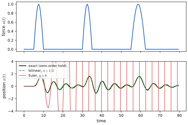
fig_S29_3. Download: PDF · SVGExample: tracking a moving object in continuous time (supplement 29.1.3)
Modify the tracking model so that energy is conserved: a particle moves on a circle, \(\dot x=y\), \(\dot y=-x\) (S29.18). In polar coordinates \(r^2=x^2+y^2\) gives \(\dot r=(x\dot x+y\dot y)/r=0\) and \(\dot\theta=(x\dot y-\dot xy)/r^2=-1\) (S29.19)–(S29.29): constant radius and constant angular speed. With observations \(\vy_t=\mH\vz_t+\bm\delta_t\), \(\bm\delta_t\sim\N(\mathbf0,0.01\mI)\), the Kalman filter with the exact discrete transition \(e^{\mathbf F\Delta}\) tracks the particle (Figure S29.4). We simulate the circle with RK2 at step 0.01 and observe at 70 times over \([0,7.5]\); the observation matrix (not legible in the supplement) is taken to be the identity, and the noise standard deviation is 0.1.
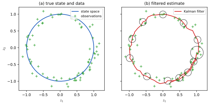
fig_S29_4. Download: PDF · SVGExample: tracking a particle in 2d (supplement 29.1.4)
A mildly nonlinear version has \(\vz'=f_z(\vz)=(z_2,\ z_1-z_1^3)^\T\) (S29.32), a particle in a double-well potential, integrated by RK2 with step \(h=0.01\) up to \(T=7.5\) and sampled at \(K=70\) times with \(\vy_t=\vz_t+\N(\mathbf0,\mR)\). The EKF predicts by integrating the mean with RK2 and the covariance by the state-transition matrix accumulated along the path, then updates linearly. The orbit we use starts at \((-1.2,0.8)\), with energy above the saddle, so it crosses both wells. The observation noise standard deviation is 0.2.
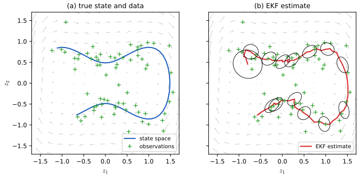
fig_S29_5. Download: PDF · SVGStructured State Space Sequence model, S4 (supplement 29.2)
supplement pp. 224–226, (S29.33)–(S29.44), Figure S29.6 The S4 model is a deep stack of (noiseless) linear SSMs. The basic layer maps an input sequence \(u(t)\in\R\) to \(y(t)\in\R\) through hidden states \(\vz(t)\in\R^N\):
\[ \dot{\vz}(t)=\mathbf A\vz(t)+\mathbf Bu(t),\qquad y(t)=\mathbf C\vz(t)+Du(t). \tag{S29.33–S29.34} \]With the bilinear rule (\(\alpha=\tfrac12\)) at step \(\Delta\), \(\vz_t=\bar{\mathbf A}\vz_{t-1}+\bar{\mathbf B}u_t\), \(y_t=\bar{\mathbf C}\vz_t\), \[ \bar{\mathbf A}=(\mI-\tfrac\Delta2\mathbf A)^{-1}(\mI+\tfrac\Delta2\mathbf A) \], \(\bar{\mathbf B}=(\mI-\tfrac\Delta2\mathbf A)^{-1}\Delta\mathbf B\), \(\bar{\mathbf C}=\mathbf C\) (S29.35)–(S29.39); the skip term \(D\) is omitted. Several such channels are processed in parallel, then a pointwise nonlinearity and a linear mixing across channels with a skip connection form one block (Figure S29.6), and blocks are stacked. Because a recurrent model samples in \(O(L)\) steps for length \(L\) (a transformer needs \(O(L^2)\)) and because it comes from a continuous-time system it can be applied at different sampling rates. The matrix \(\mathbf A\) has a special structure (HiPPO) so that \(\vz_t\) compresses the history compactly and the update costs \(O(N)\) per step.
Filling the gap 29.21: a linear SSM layer is a causal convolution supplement p. 226, (S29.40)–(S29.44)
This is why training is parallel: the recurrence is replaced by a convolution that an FFT computes.
Derivation
Start from \(\vz_{-1}=\mathbf0\) and unroll: \(\vz_t=\sum_{j=0}^t\bar{\mathbf A}^{t-j}\bar{\mathbf B}u_j\) by induction (\(\vz_0=\bar{\mathbf B}u_0\), and \(\vz_t=\bar{\mathbf A}\vz_{t-1}+\bar{\mathbf B}u_t\)), so
\[ y_k=\bar{\mathbf C}\vz_k=\sum_{j=0}^k\bar{\mathbf C}\bar{\mathbf A}^{k-j}\bar{\mathbf B}\,u_j=(\mathbf K*\mathbf u)_k,\qquad \mathbf K=(\bar{\mathbf C}\bar{\mathbf B},\ \bar{\mathbf C}\bar{\mathbf A}\bar{\mathbf B},\dots,\bar{\mathbf C}\bar{\mathbf A}^{L-1}\bar{\mathbf B}). \](the book writes \(y=K\odot u\); the operation is convolution, not an elementwise product). Once \(\mathbf K\) is known, the whole output is computed in \(O(L\log L)\) by the FFT (zero-padding to length \(2L\) to avoid wrap-around); the difficulty the supplement mentions is computing \(\mathbf K\) quickly for a huge state, which S4 solves with the structure of \(\mathbf A\) in \(O(N+L)\) time and space. The recurrence and the convolution give the same sequence (confirmed for a random stable \(\bar{\mathbf A}\) to \(10^{-12}\)). ∎
Practice problems
Chapter 29 of the book has no end-of-chapter exercises. Here are three short problems with worked solutions (numbers computed with the code).
Problem 29.1. A state of an HMM is replaced by a chain of \(n\) states with self-loop probability \(p=0.9\), as in Section 29.5.1. (a) Find the mean and variance of the duration for \(n=3\). (b) Find the probability that the duration exceeds 30, and compare it with a plain geometric duration of the same mean. (c) How many chained states are needed to bring the coefficient of variation of the duration down to 0.2?
Solution
(a) \(\E D=n/(1-p)=30\), \(\var D=np/(1-p)^2=270\) (Filling the gap 29.7), standard deviation 16.4. (b) \(P(D>30)=1-\sum_{d=3}^{30}\binom{d-1}{2}0.9^{d-3}0.1^3=0.411\). A geometric duration with the same mean 30 has \(P(D>30)=(1-1/30)^{30}=0.362\), and standard deviation \(\sqrt{p'}/(1-p')=29.5\) with \(p'=29/30\): the chain concentrates the law (sd 16 instead of 29). (c) The coefficient of variation is \(\sqrt{\var D}/\E D=\sqrt{np}/(1-p)\cdot(1-p)/n=\sqrt{p/n}\), independent of the common factor; \(\sqrt{0.9/n}\le0.2\) needs \(n\ge22.5\), so \(n=23\) (CV 0.198, mean 230 steps). Larger \(n\) buys a sharper duration at the price of \(n\) states per regime, which is why the explicit-duration model is preferred for long, regular durations.
Problem 29.2. A local level model has \(\sigma_y=1\) and \(\sigma_\mu^2=0.1\). Find the steady-state gain, the effective memory of the filter, and the standard deviation of the 12-step-ahead forecast.
Solution
With \(q=\sigma_\mu^2/\sigma_y^2=0.1\) (Filling the gap 29.15): \(P/\sigma_y^2=\tfrac12(q+\sqrt{q^2+4q})=0.3702\), gain \(k=P/(P+\sigma_y^2)=0.2702\), so the filter is exponential smoothing with \(\alpha=0.27\) and effective memory \(1/k=3.7\) observations. The steady-state filtered variance is \(P\sigma_y^2/(P+\sigma_y^2)=0.2702\), so the 12-step forecast variance is \(0.2702+12\times0.1+1=2.470\) and its sd is 1.57 (a random-walk level makes the variance grow by \(\sigma_\mu^2\) per step, linearly, in contrast with an observation-noise floor of 1). Increasing \(\sigma_\mu^2\) to 1 raises the gain to 0.618 and shortens the memory to 1.6 observations.
Problem 29.3. In recursive least squares with prior \(\vw\sim\N(\mathbf0,100\mI_2)\) and noise variance \(\sigma^2=1\), the first example is \(\vx_1=(1,2)^\T\). Compute the Kalman gain and the posterior covariance. Along which directions does the posterior shrink?
Solution
The gain is \[ \mK_1=\bSig_0\vx_1/(\sigma^2+\vx_1^\T\bSig_0\vx_1)=100(1,2)^\T/501=(0.1996,0.3992)^\T \], since \(\vx_1^\T\bSig_0\vx_1=100\cdot5=500\). The posterior covariance is
\[ \bSig_1=\bSig_0-\frac{\bSig_0\vx_1\vx_1^\T\bSig_0}{501}=\begin{pmatrix}80.04&-39.92\\-39.92&20.16\end{pmatrix}. \]Along \(\vx_1\) the variance of \(\vx_1^\T\vw\) drops from 500 to \(500/501=0.998\) (the data pin the prediction at \(\vx_1\) down to roughly the noise level), while along the orthogonal direction \((2,-1)^\T\) the variance of \((2,-1)\vw\) is still 500 (the quadratic form \(4\cdot80.04+4\cdot39.92+20.16\) equals 500.0): one example says nothing about the other direction. LMS would instead use the gain \(\eta\vx_1\) along \(\vx_1\) only and no memory of the remaining uncertainty.
Demonstrations for this chapter
Each demonstration runs in the browser, with seeded or exported data, and links back to these notes. Their numbers (log-likelihoods, run-length posteriors, forecasts) are those of the Python code.
| Demonstration | What you can see | Sections |
|---|---|---|
| Baum–Welch (EM) for a hidden Markov model | EM on the casino rolls: log-likelihood, estimated emissions against the true ones, smoothed state probabilities. Presets: 1 a poor start; 2 1000 rolls; 3 only 50 rolls; 4 identical states (a fixed point); 5 three states for a two-state casino. | 29.4.1, 29.4.2 |
| Bayesian online changepoint detection | The run-length posterior of BOCPD with hazard, prior variance and noise variance sliders. Presets: 1 Figure 29.22 series; 2 no change; 3 large hazard; 4 tiny hazard; 5 outliers read as changes. | 29.5.6 |
| Structural time series: trend, season and forecast | Local linear trend plus seasonal model of CO2 with the four noise standard deviations as sliders: log-likelihood, ten-year forecast, smoothed components, predictive z-scores. Presets: 1 maximum likelihood; 2 rigid trend; 3 flexible trend; 4 evolving season; 5 components. | 29.12.2, 29.12.4, 29.12.5.1 |
The Python code that produces every figure of this page is code/ch29_state_space_models.py (see the code index). The Kalman filtering of Figure 29.23 is in the demonstration of Chapter 8.
Errors and slips found in the book
Everything below was confirmed by recomputation. Items marked (minor) are notational.
- (29.28), (29.32), Algorithm 29.1: \(\E[N_k]\) is summed over \(t=2,\dots,T\), but the emission update (29.32) divides sums over \(t=1,\dots,T\) by it; the denominator must run over all \(t\), otherwise the rows of \(\hat{\mathbf B}\) do not sum to one (Filling the gap 29.3).
- (29.50): the geometric duration on \(d\ge1\) is \((1-A_{ii})A_{ii}^{d-1}\), not \((1-A_{ii})A_{ii}^d\) (Filling the gap 29.7).
- (29.82): \(\mH=\begin{pmatrix}1&0&0&0\\0&0&1&0\end{pmatrix}\) extracts \((u,\dot u)\); with the state ordering \((u,v,\dot u,\dot v)\) of (29.81) it must be \(\begin{pmatrix}1&0&0&0\\0&1&0&0\end{pmatrix}\).
- Section 29.7.2: the LMS update corresponds to a gain \(\mK_t\approx\eta_t\vx_t\), not \(\eta_t\mathbf1\).
- Section 29.2.5: a pure 7-degree rotation \(\mathbf E_j\) has eigenvalues of modulus 1, so the observations do not converge to \((\mI-\mathbf E_j)^{-1}\bmu_j\) as claimed; the damped rotation \(0.93\,\mathbf R(7^\circ)\) with \(\|\bmu_j\|=0.59\) reproduces the quoted attractors (Filling the gap 29.1).
- (29.173): the KL penalty is the one-step KL averaged over a sampled \(\vz_{t-1}\), which is at least the exact \(d\)-step KL by Jensen, so the stated bound is valid but looser than the \(d\)-step bound (Filling the gap 29.19).
- Section 29.3.1 and Figure 29.8: the quantity plotted and called the marginal likelihood is the maximised log-likelihood (29.21), which cannot decrease with the number of states except through local optima; the decline attributed to a Bayesian Occam's razor appears only once the rate prior is included (log posterior \(-228.8,-228.9,-229.1\) for \(K=4,5,6\) against a flat log-likelihood), and comes from the prior and the fixed switching probabilities rather than from integrating over the rates.
- Section 29.5.4: exact inference in a coupled HMM costs \(O(T(K^M)^2)\), not \(O(T(KM)^2)\).
- (S29.2) and the text above it: the integral must run over \([t_i,t_{i+1}]\) and give \(z_{i+1}\) (the text has \(\int_{t_{i-1}}^{t_i}\) and "to compute \(z_i\) from \(z_{i-1}\)"). (S29.43): the layer output is a convolution \(\mathbf K*\mathbf u\), not an elementwise product (Filling the gap 29.21).
- (minor) (29.10) uses \(y_{jk}\) for the emission matrix, which clashes with the observation \(\vy\); (29.89)–(29.91) are printed with the signs and the range of the sums partly lost; (29.103) writes \(\mathbf P_{t-1,t}\) where \(\mathbf P_{t,t-1}^\T\) is meant; the book's (29.99), (29.104) are correct once the new \(\mathbf A^{\mathrm{new}}\) is used as stated.
References
- Murphy, K. P. (2023). Probabilistic Machine Learning: Advanced Topics. MIT Press. Chapter 29 (pp. 1013–1076) and Supplementary Chapter 29 (pp. 219–226). probml.github.io/pml-book/book2.html.
- Adams, R. P. and MacKay, D. J. C. (2007). Bayesian online changepoint detection. arXiv:0710.3742.
- Baum, L. E., Petrie, T., Soules, G. and Weiss, N. (1970). A maximization technique occurring in the statistical analysis of probabilistic functions of Markov chains. Annals of Mathematical Statistics, 41(1), 164–171.
- Brodersen, K. H., Gallusser, F., Koehler, J., Remy, N. and Scott, S. L. (2015). Inferring causal impact using Bayesian structural time-series models. Annals of Applied Statistics, 9(1), 247–274.
- Durbin, J. and Koopman, S. J. (2012). Time Series Analysis by State Space Methods, 2nd edition. Oxford University Press.
- Durbin, R., Eddy, S., Krogh, A. and Mitchison, G. (1998). Biological Sequence Analysis. Cambridge University Press.
- Fearnhead, P. and Liu, Z. (2007). On-line inference for multiple changepoint problems. Journal of the Royal Statistical Society B, 69(4), 589–605.
- Gu, A., Goel, K. and Ré, C. (2022). Efficiently modeling long sequences with structured state spaces. ICLR.
- Hafner, D., Lillicrap, T., Fischer, I., Villegas, R., Ha, D., Lee, H. and Davidson, J. (2019). Learning latent dynamics for planning from pixels. ICML.
- Hsu, D., Kakade, S. M. and Zhang, T. (2012). A spectral algorithm for learning hidden Markov models. Journal of Computer and System Sciences, 78(5), 1460–1480.
- Ho, B. L. and Kalman, R. E. (1966). Effective construction of linear state-variable models from input/output functions. Regelungstechnik, 14, 545–548.
- Krishnan, R. G., Shalit, U. and Sontag, D. (2017). Structured inference networks for nonlinear state space models. AAAI.
- Shumway, R. H. and Stoffer, D. S. (1982). An approach to time series smoothing and forecasting using the EM algorithm. Journal of Time Series Analysis, 3(4), 253–264.
- Särkkä, S. (2013). Bayesian Filtering and Smoothing. Cambridge University Press.
- Siddiqi, S., Boots, B. and Gordon, G. (2007). A constraint generation approach to learning stable linear dynamical systems. NIPS.
- Van Overschee, P. and De Moor, B. (1996). Subspace Identification for Linear Systems. Kluwer.
- Chung, J., Kastner, K., Dinh, L., Goel, K., Courville, A. and Bengio, Y. (2015). A recurrent latent variable model for sequential data. NIPS.
The numerical statements in the text (HMM forwards–backwards and Viterbi against enumeration of all paths, the gradient as expected counts, the EM monotonicity and M step, the negative binomial duration law, the spectral operators, the BOCPD recursion against all segmentations, the Kalman filter, smoother and lag-one covariances against the joint Gaussian, the EM updates for the LDS, recursive least squares, the white-noise-acceleration covariance, subspace identification, the local level and local linear trend forecasts, the causal-impact covariance, the Laplace EM for the Poisson LDS, the deep-SSM bounds, the exact SLDS filter, and the discretisation and convolution facts of the supplement) were confirmed numerically.