Approximate Inference
When the posterior cannot be computed, we replace it by the closest member of a tractable family. This chapter builds the two deterministic ways of doing so, variational inference (minimise \(\KL(q\|p)\) and obtain a lower bound on the evidence) and expectation propagation (match moments factor by factor, a local \(\KL(p\|q)\)), and works every example of the book through to the last line.
Ch. 1 Introduction Ch. 2 Probability distributions Ch. 3 Linear regression Ch. 4 Linear classification Ch. 5 Neural networks Ch. 6 Kernel methods Ch. 7 Sparse kernel machines Ch. 8 Graphical models Ch. 9 Mixture models and EM Ch. 10 Approximate inference Ch. 11 Sampling methods Ch. 12 Continuous latent variables Ch. 13 Sequential data Ch. 14 Combining models
How to read these notes
They follow the book. Sections carry Bishop's numbers (10.1, 10.2.1, ...) and every displayed equation that appears in the book carries the book's own equation number, e.g. (10.9), so you can read these notes next to the book. Equations without a number are steps that the book skips.
Filling the gaps. Wherever the book says that a result "can be shown", "is easily verified", is obtained "after some manipulation" or is left as an exercise, an orange Filling the gap box gives the full argument. Proofs and derivations start hidden: open one with its bar, or use the button below. Every exercise of the chapter is solved in the Exercises section.
Figures and demonstrations. Every numerical figure of the chapter is reproduced from scratch by the Python code, and the ▶ Demo boxes open an interactive demonstration already set to the case being discussed. Standard identities (KL divergence, completing the square, Gaussian, Gamma, Dirichlet and Wishart facts, convex conjugates) are proved once in the mathematical toolkit.
Main reference
C. M. Bishop, Pattern Recognition and Machine Learning, Springer (2006), Chapter 10, pages 461–522. Section, equation, figure and exercise numbers below refer to this book. Further reading is listed in the references.
Printings. Chapter 10 had many corrections after the first printing (Bishop's errata list). The notes always state the corrected equation and add a short Erratum note naming the original. Four further points are not in the errata list and are flagged where they occur: (10.63) should read \(\nu_k=\nu_0+N_k\) (some printings, including the one used here, add a 1); the normaliser in (10.116); the conventions behind (10.222) and (10.223) for the clutter problem; and the word "convex" on p. 466, which should be "concave".
The explanations, derivations and code are my own; equations are cited by their numbers in the book.
The chapter at a glance
| Method | What is approximated | Criterion | Sections |
|---|---|---|---|
| Global variational inference (mean field, variational Bayes) | the whole posterior, by a factorised \(q(\mathbf{Z})\) | maximise the lower bound \(\LB(q)\), equivalently minimise \(\KL(q\|p)\) | 10.1–10.4 |
| Local variational bounds | one awkward factor at a time (e.g. the logistic sigmoid), by a bound with its own parameter \(\xi\) | maximise the resulting bound on the evidence over \(\xi\) | 10.5, 10.6 |
| Expectation propagation | each factor \(f_i\) of the joint, by an exponential-family factor \(\tilde f_i\) | match the moments of \(q^{\setminus i}f_i\) (a local \(\KL(p\|q)\)) | 10.7 |
All three are deterministic and give a closed-form, fast approximation, in contrast to the sampling methods of Chapter 11, which are exact in the limit of infinite computation. The Laplace approximation of Section 4.4 is the simplest member of the family: it is local, built from the curvature at one mode, whereas the methods here use the whole distribution.
Throughout, \(\mathbf{X}\) denotes all observed variables and \(\mathbf{Z}\) all unobserved ones: latent variables and, in a fully Bayesian model, the parameters too. The model is the joint density \(p(\mathbf{X},\mathbf{Z})\), which we can evaluate. What we want, the posterior \(p(\mathbf{Z}\given\mathbf{X})\) and the evidence \(p(\mathbf{X})\)
10.1 Variational inference
A functional maps a function to a number. The example of the book is the entropy
\[ \mathrm{H}[p]=-\int p(x)\ln p(x)\,\d x . \tag{10.1} \]Erratum. The first printing omits the minus sign in (10.1).
The functional derivative \(\delta F/\delta q(x)\) says how \(F[q]\) changes when \(q\) is perturbed near \(x\): \(F[q+\epsilon\eta]\)
Result 10.1 (the evidence decomposition) p. 463, (10.2)–(10.4)
For any density \(q(\mathbf{Z})\) (sums replace integrals for discrete variables),
\[ \ln p(\mathbf{X})=\LB(q)+\KL(q\|p) \tag{10.2} \] \[ \LB(q)=\int q(\mathbf{Z})\ln\left\{\frac{p(\mathbf{X},\mathbf{Z})}{q(\mathbf{Z})}\right\}\d\mathbf{Z} \tag{10.3} \] \[ \KL(q\|p)=-\int q(\mathbf{Z})\ln\left\{\frac{p(\mathbf{Z}\given\mathbf{X})}{q(\mathbf{Z})}\right\}\d\mathbf{Z}. \tag{10.4} \]Hence \(\LB(q)\le\ln p(\mathbf{X})\) for every \(q\), with equality if and only if \(q(\mathbf{Z})\)
Proof
By the product rule \(p(\mathbf{X},\mathbf{Z})\)
Multiply by \(q(\mathbf{Z})\) and integrate over \(\mathbf{Z}\). The last term does not depend on \(\mathbf{Z}\) and \(\int q\,\d\mathbf{Z}=1\), so it contributes \(\ln p(\mathbf{X})\); the other two terms are \(\LB(q)\) and \(-\KL(q\|p)\). This is (10.2).
By Gibbs' inequality (toolkit: KL divergence), \(\KL(q\|p)\ge0\) with equality if and only if \(q=p(\cdot\given\mathbf{X})\) almost everywhere. In one line, by Jensen's inequality for the concave logarithm, \(-\KL(q\|p)\)
The point of (10.2) is that \(\LB(q)\) involves only the joint \(p(\mathbf{X},\mathbf{Z})\), which we can evaluate, while the KL term involves the unknown posterior. So we can make the KL small by making \(\LB\) large without ever computing \(p(\mathbf{Z}\given\mathbf{X})\). The identity is the same as (9.70) in the EM chapter, except that the parameters are now random and live inside \(\mathbf{Z}\). Two further remarks. First, \(\LB\) is a concave functional of \(q\) (the entropy \(-\int q\ln q\) is strictly concave and \(\int q\ln p\) is linear), so over any convex family of densities it has a unique maximiser. Second, the family is restricted purely for tractability: a richer family can only get closer to the posterior, so there is no over-fitting in choosing a flexible \(q\).
The simplest restriction is a parametric family \(q(\mathbf{Z}\given\bm\omega)\), for instance a Gaussian, with \(\LB\) maximised over \(\bm\omega\) by ordinary optimisation. Figure 10.1 does this for the skewed density of Figure 4.14, \(p(z)\propto e^{-z^2/2}\sigma(20z+4)\). The next result explains what the optimal Gaussian is.
Result 10.2 (the best Gaussian in the sense of \(\KL(q\|p)\))
Let \(p(z)=\tilde p(z)/Z\) on \(\R\) with \(\ln\tilde p\) twice differentiable (derivatives of at most polynomial growth), and let \(q(z)=\N(z\given m,s^2)\). Then
\[ \LB(m,s^2)=\E_q[\ln\tilde p(z)]+\tfrac12\ln(2\pi e s^2)=\ln Z-\KL(q\|p), \]and at any stationary point
\[ \E_q\big[(\ln\tilde p)'(z)\big]=0,\qquad \E_q\big[(\ln\tilde p)''(z)\big]=-\frac{1}{s^2}. \]Compare the Laplace approximation (Section 4.4), which imposes the same two equations at the mode: \((\ln\tilde p)'(z_0)=0\) and \(s^2=-1/(\ln\tilde p)''(z_0)\). The variational Gaussian replaces point evaluations by averages over \(q\) itself.
Proof
The entropy of \(\N(m,s^2)\) is \(\frac12\ln(2\pi e s^2)\) (toolkit: Gaussian facts), and \(\int q\ln(\tilde p/q)\)
and setting both to zero gives the two conditions. ∎
For the density of Figure 10.1 I computed the three Gaussians by numerical integration (the numbers below were computed for these notes and are not from the book):
| Gaussian | mean | variance | \(\KL(q\|p)\) | \(\KL(p\|q)\) |
|---|---|---|---|---|
| exact moments of \(p\) (= expectation propagation, Section 10.7) | 0.673 | 0.414 | 0.367 | 0.117 |
| Laplace (mode and curvature) | 0.078 | 0.393 | 2.377 | 0.569 |
| variational (maximise \(\LB\)) | 0.707 | 0.244 | 0.172 | 0.204 |
Each criterion wins on its own divergence. The variational Gaussian sits in the bulk of the mass but is narrower than \(p\); the Laplace Gaussian is centred at the mode, near the steep left edge, and so leaks mass into the region where \(p\) is almost zero, which \(\KL(q\|p)\) punishes heavily.
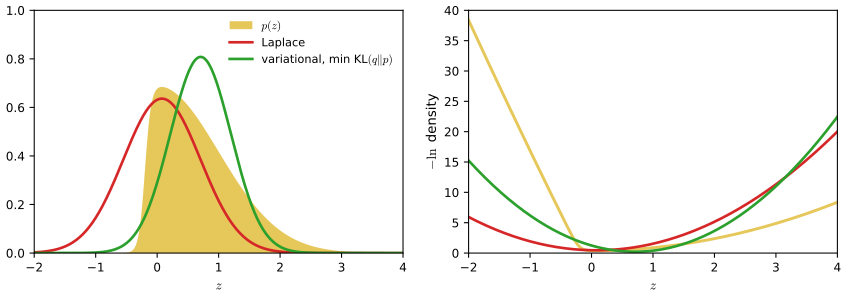
fig10_1. Download: PDF · SVG10.1.1 Factorised distributions
The second way to restrict \(q\) leaves the functional form free but imposes independence between groups. Partition \(\mathbf{Z}\) into disjoint groups \(\mathbf{Z}_1,\dots,\mathbf{Z}_M\) and take
\[ q(\mathbf{Z})=\prod_{i=1}^{M}q_i(\mathbf{Z}_i). \tag{10.5} \]This is the mean-field family of statistical physics. Nothing is assumed about the individual factors \(q_i\); their forms will come out of the optimisation. Write \(q_j\) for \(q_j(\mathbf{Z}_j)\), and \(\E_{i\ne j}[\cdot]\) for the expectation over all factors except the \(j\)th:
\[ \E_{i\ne j}[\ln p(\mathbf{X},\mathbf{Z})]=\int\ln p(\mathbf{X},\mathbf{Z})\prod_{i\ne j}q_i\,\d\mathbf{Z}_i . \tag{10.8} \]Result 10.3 (the mean-field update) pp. 464–466, (10.6)–(10.9)
Fix all factors except \(q_j\). Define the normalised density
\[ \tilde p(\mathbf{X},\mathbf{Z}_j)=\frac{\exp\big(\E_{i\ne j}[\ln p(\mathbf{X},\mathbf{Z})]\big)}{\mathcal{Z}_j},\qquad \mathcal{Z}_j=\int\exp\big(\E_{i\ne j}[\ln p(\mathbf{X},\mathbf{Z})]\big)\,\d\mathbf{Z}_j , \]so that \(\ln\tilde p(\mathbf{X},\mathbf{Z}_j)\)
so the unique maximiser over \(q_j\) (all densities on the space of \(\mathbf{Z}_j\)) is
\[ \ln q_j^\star(\mathbf{Z}_j)=\E_{i\ne j}[\ln p(\mathbf{X},\mathbf{Z})]+\const,\qquad q_j^\star(\mathbf{Z}_j)=\frac{\exp\big(\E_{i\ne j}[\ln p(\mathbf{X},\mathbf{Z})]\big)}{\int\exp\big(\E_{i\ne j}[\ln p(\mathbf{X},\mathbf{Z})]\big)\,\d\mathbf{Z}_j}. \tag{10.9} \]The update is a global maximum in its own factor (not merely a stationary point), and after the update \(\LB\)
Filling the gap: from (10.3) to (10.9) pp. 464–466
The book "dissects out" \(q_j\) in two lines and then "recognises" a KL divergence. Here are all the steps, including what the constants are.
Derivation
Step 1 (substitute). With \(q=\prod_iq_i\), \(\ln q=\sum_i\ln q_i\), and (10.3) becomes
\[ \LB(q)=\int\prod_iq_i\Big\{\ln p(\mathbf{X},\mathbf{Z})-\sum_i\ln q_i\Big\}\d\mathbf{Z}. \]Step 2 (the energy term). By Fubini's theorem, integrate first over all groups except \(\mathbf{Z}_j\):
\[ \int\prod_iq_i\ln p(\mathbf{X},\mathbf{Z})\,\d\mathbf{Z}=\int q_j\Big\{\int\ln p(\mathbf{X},\mathbf{Z})\prod_{i\ne j}q_i\,\d\mathbf{Z}_i\Big\}\d\mathbf{Z}_j=\int q_j\,\E_{i\ne j}[\ln p(\mathbf{X},\mathbf{Z})]\,\d\mathbf{Z}_j . \]Step 3 (the entropy term). For each \(i\), \(\int\prod_kq_k\ln q_i\,\d\mathbf{Z}\)
The last sum does not involve \(q_j\): it is the "const" of (10.6).
Step 4 (recognise a KL divergence). Since \(\E_{i\ne j}[\ln p]\)
Step 5 (maximise). Only the KL term depends on \(q_j\), and by Gibbs' inequality it is \(\ge0\) with equality exactly when \(q_j=\tilde p\). Hence \(q_j^\star=\tilde p\), which is (10.9) together with its normalised form. The maximum is attained, unique and global over all densities for \(\mathbf{Z}_j\). (We need \(\mathcal{Z}_j\lt\infty\), which holds in all the models of this chapter.) ∎
The same result by calculus of variations. Add a Lagrange multiplier for \(\int q_j=1\) and take the functional derivative (toolkit: optimising over distributions):
\[ \frac{\delta}{\delta q_j}\Big\{\int q_j\E_{i\ne j}[\ln p]\,\d\mathbf{Z}_j-\int q_j\ln q_j\,\d\mathbf{Z}_j+\lambda\Big(\int q_j\,\d\mathbf{Z}_j-1\Big)\Big\}=\E_{i\ne j}[\ln p]-\ln q_j-1+\lambda=0, \]so \(q_j\)
In practice we never compute \(\mathcal{Z}_j\) first. We write \(\ln p(\mathbf{X},\mathbf{Z})\), keep only the terms that involve \(\mathbf{Z}_j\) (everything else is absorbed into "const"), take expectations over the other factors, and recognise the result as the logarithm of a standard density; the normaliser is then read off. Every example below follows this recipe.
Result 10.4 (coordinate ascent never decreases the bound) p. 466
Cycle through \(j=1,\dots,M\), replacing \(q_j\) by \(q_j^\star\) of (10.9) computed from the current values of the other factors. Then the sequence of values of \(\LB\) is non-decreasing and bounded above by \(\ln p(\mathbf{X})\), so it converges.
Proof
Each update maximises \(\LB\) over \(q_j\) with the others held fixed (Result 10.3), so it cannot decrease \(\LB\). By Result 10.1, \(\LB\le\ln p(\mathbf{X})\). A non-decreasing sequence bounded above converges. ∎
Note on p. 466. The book says convergence holds "because bound is convex with respect to each of the factors". The property used is that \(\LB\) is concave in each factor (Result 10.3), so that each update is a global maximum in that factor. Convergence is of the values of \(\LB\); the limit is in general only a local maximum of \(\LB\) over the product family, because \(\LB\) is not jointly concave in \((q_1,\dots,q_M)\), and different starts can end at different solutions (Figure 10.3).
Algorithm 10.1 (coordinate ascent variational inference)
- Choose the factorisation (10.5) and initialise the factors (in practice only the expectations that the updates need).
- For \(j=1,\dots,M\): compute \(\E_{i\ne j}[\ln p(\mathbf{X},\mathbf{Z})]\) as a function of \(\mathbf{Z}_j\), recognise it as \(\ln\) of a known density up to a constant, and set \(q_j\) to that density (10.9).
- Evaluate \(\LB(q)\). It must not decrease: a decrease signals an error in the derivation or the code.
- Repeat steps 2–3 until the increase in \(\LB\) is below a tolerance.
10.1.2 Properties of factorised approximations
To see what the factorisation costs, approximate a correlated Gaussian \(p(\mathbf{z})\)
Filling the gap: the optimal factors (10.11)–(10.15) p. 467
The book completes the square in one line. All the steps:
Derivation
Up to a constant, \(\ln p(\mathbf{z})\)
By (10.9), \(\ln q_1^\star(z_1)\)
This is a quadratic in \(z_1\) of the form \(-\frac12 Az_1^2+bz_1\) with \(A=\Lambda_{11}\gt0\) (a diagonal element of a positive definite matrix) and \(b\)
Exchanging the roles of the two coordinates,
\[ q_2^\star(z_2)=\N(z_2\given m_2,\Lambda_{22}^{-1}) \tag{10.14} \] \[ m_2=\mu_2-\Lambda_{22}^{-1}\Lambda_{21}\big(\E[z_1]-\mu_1\big). \tag{10.15} \]Gaussianity was not assumed: it is forced by the quadratic form of \(\ln p\). Note also that (10.13) is exactly the conditional mean \(\E_p[z_1\given z_2]\) evaluated at \(z_2=\E[z_2]\), and \(\Lambda_{11}^{-1}\) is the conditional variance \(\var_p[z_1\given z_2]\) (toolkit: partitioned Gaussians). ∎
Erratum. In the first printing the left side of (10.12) reads \(q^\star(z_1)\) instead of \(q_1^\star(z_1)\).
Result 10.5 (mean field on a Gaussian: right means, too little variance) p. 467, Exercise 10.2
Let \(\rho\) be the correlation of \(z_1,z_2\) under \(p\). Then (a) if \(\bm\Lambda\) is non-singular, the only solution of (10.13) and (10.15) is \(\E[z_1]=\mu_1\), \(\E[z_2]=\mu_2\); (b) the variance of \(q_i^\star\) is
\[ \Lambda_{ii}^{-1}=(1-\rho^2)\,\Sigma_{ii}\ \le\ \Sigma_{ii}, \]the conditional variance of \(z_i\), not the marginal variance \(\Sigma_{ii}\) (\(\bm\Sigma=\bm\Lambda^{-1}\)), with equality only if \(\rho=0\); (c) cycling through (10.13) and (10.15) multiplies the error in the means by \(\rho^2\)
Proof
(a) Put \(e_i=\E[z_i]-\mu_i\). Using \(\E[z_i]=m_i\), (10.13) and (10.15) read \(e_1\)
(b) For a \(2\times2\) matrix, \(\bm\Sigma\)
(c) One sweep updates \(e_1'\)
The same holds in \(D\) dimensions: each mean-field factor of a Gaussian has variance \(1/\Lambda_{ii}\)
The reverse divergence. Expectation propagation (Section 10.7) minimises \(\KL(p\|q)\) instead. For a factorised \(q\),
\[ \KL(p\|q)=-\int p(\mathbf{Z})\Big[\sum_{i=1}^{M}\ln q_i(\mathbf{Z}_i)\Big]\d\mathbf{Z}+\const \tag{10.16} \]where the constant is \(\int p\ln p=-\mathrm{H}[p]\) (the book calls it the entropy; it is minus the entropy).
Result 10.6 (\(\KL(p\|q)\) over factorised \(q\) gives the marginals) p. 468, (10.17), Exercise 10.3
Let \(p_i(\mathbf{Z}_i)\)
so the minimiser is unique and closed-form, with no iteration:
\[ q_j^\star(\mathbf{Z}_j)=\int p(\mathbf{Z})\prod_{i\ne j}\d\mathbf{Z}_i=p_j(\mathbf{Z}_j). \tag{10.17} \]Proof
In (10.16), \(\int p(\mathbf{Z})\ln q_i(\mathbf{Z}_i)\,\d\mathbf{Z}\)
The bracket equals \(\int p\ln\big(p/\prod_ip_i\big)\)
For the Gaussian, the marginals are \(\N(z_i\given\mu_i,\Sigma_{ii})\) (2.98): again the right means, but now the full marginal variances, so \(q\) puts substantial mass where \(p\) is small, outside the narrow correlated ellipse (Figure 10.2b). The first term \(\KL(p\|\prod_ip_i)\) is the multi-information of \(p\): the irreducible error of any factorised approximation under this divergence.
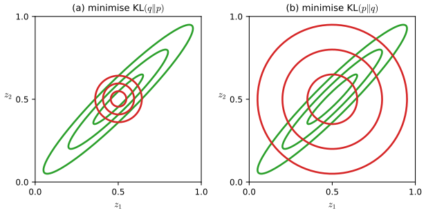
fig10_2. Download: PDF · SVGZero-forcing and zero-avoiding. In
\[ \KL(q\|p)=-\int q(\mathbf{Z})\ln\left\{\frac{p(\mathbf{Z})}{q(\mathbf{Z})}\right\}\d\mathbf{Z} \tag{10.18} \]the integrand \(q\ln(q/p)\) is huge wherever \(p\approx0\) but \(q\) is not, so the minimiser keeps \(q\approx0\) wherever \(p\approx0\): it is zero-forcing, it under-estimates the support of \(p\), and on a multimodal \(p\) it settles on one mode. In \(\KL(p\|q)=\int p\ln(p/q)\) the penalty is large wherever \(p\gt0\) but \(q\approx0\), so \(q\) must cover all of the mass of \(p\): it is zero-avoiding. For a single Gaussian \(q\) the minimiser of \(\KL(p\|q)\) matches the overall mean and covariance of \(p\) (Result 10.27 below), which for a bimodal \(p\) puts the peak of \(q\) between the modes (Figure 10.3a), while \(\KL(q\|p)\) has one local minimum per mode (Figures 10.3b, c). In a mixture model the modes are the \(K!\) relabellings (Section 10.2.4) and averaging over them would be useless, which is why variational Bayes, not expectation propagation, is used for mixtures.
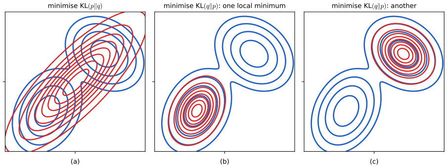
fig10_3. Download: PDF · SVGDefinition 10.1 (the alpha family of divergences) p. 470, (10.19)
For densities \(p,q\) and \(-\infty\lt\alpha\lt\infty\), \(\alpha\ne\pm1\),
\[ \mathrm{D}_\alpha(p\|q)=\frac{4}{1-\alpha^2}\left(1-\int p(x)^{(1+\alpha)/2}\,q(x)^{(1-\alpha)/2}\,\d x\right). \tag{10.19} \](Ali and Silvey 1966; Amari 1985; Minka 2005.) At \(\alpha=0\) it is linked to the Hellinger distance
\[ \mathrm{D}_{\mathrm H}(p\|q)=\int\big(p(x)^{1/2}-q(x)^{1/2}\big)^2\,\d x. \tag{10.20} \]Erratum. In the first printing the integrand of (10.20) is not squared.
Result 10.7 (properties of the alpha family) p. 470, Exercise 10.6
(a) \(\mathrm{D}_\alpha(p\|q)\ge0\) for every \(\alpha\), with equality iff \(p=q\). (b) \(\mathrm{D}_\alpha(p\|q)\)
Proof
Put \(a=(1+\alpha)/2\), so \((1-\alpha)/2=1-a\), \(1-\alpha^2=4a(1-a)\) and \(\mathrm{D}_\alpha\)
(a) If \(0\lt a\lt1\) (\(|\alpha|\lt1\)), \(t\mapsto t^a\) is concave, so by Jensen \(I(a)\)
(b) (The route suggested in Exercise 10.6.) As \(\alpha\to1\), \(\epsilon=1-a\to0\) and \(I\)
(c) At \(\alpha=0\), \(\mathrm{D}_0=4(1-\int\sqrt{pq})\), while \(\mathrm{D}_{\mathrm H}\)
(d) For \(a\lt0\) the integrand \(p^aq^{1-a}\) is infinite where \(p=0\lt q\), so any \(q\) with \(\mathrm{D}_\alpha\lt\infty\) vanishes where \(p\) does (and \(a=0\) is the limit \(\KL(q\|p)\), which behaves the same way). For \(a\gt1\) the factor \(q^{1-a}\) is infinite where \(q=0\lt p\), so \(q\) must be positive wherever \(p\) is (and \(a=1\) is \(\KL(p\|q)\)). ∎
Minka (2005) shows that variational message passing (\(\alpha=-1\)), loopy belief propagation and expectation propagation (\(\alpha=1\)), and fractional and power EP (other \(\alpha\)) are all local minimisations of members of this family (Bishop, p. 517).
10.1.3 Example: the univariate Gaussian
Data \(\mathcal{D}=\{x_1,\dots,x_N\}\) are iid \(\N(\mu,\tau^{-1})\) with unknown mean \(\mu\) and precision \(\tau\) (MacKay 2003):
\[ p(\mathcal{D}\given\mu,\tau)=\Big(\frac{\tau}{2\pi}\Big)^{N/2}\exp\Big\{-\frac\tau2\sum_{n=1}^{N}(x_n-\mu)^2\Big\} \tag{10.21} \] \[ p(\mu\given\tau)=\N\big(\mu\given\mu_0,(\lambda_0\tau)^{-1}\big) \tag{10.22} \] \[ p(\tau)=\Gam(\tau\given a_0,b_0). \tag{10.23} \]This Gaussian–Gamma prior is conjugate, so the exact posterior is again Gaussian–Gamma (Exercise 2.44) and we can compare. The mean-field approximation is
\[ q(\mu,\tau)=q_\mu(\mu)\,q_\tau(\tau). \tag{10.24} \]The true posterior does not factorise, because the precision of \(\mu\) given \(\tau\) is proportional to \(\tau\).
Filling the gap: the factor \(q_\mu\) p. 471 (10.25)–(10.27) Exercise 10.7
Derivation
By (10.9),
\[ \ln q_\mu^\star(\mu)=\E_\tau[\ln p(\mathcal{D}\given\mu,\tau)+\ln p(\mu\given\tau)+\ln p(\tau)]+\const, \]and \(\ln p(\tau)\) does not involve \(\mu\). The two remaining logarithms are
\[ \ln p(\mathcal{D}\given\mu,\tau)=\tfrac N2\ln\tau-\tfrac N2\ln2\pi-\tfrac\tau2\sum_n(x_n-\mu)^2, \] \[ \ln p(\mu\given\tau)=\tfrac12\ln(\lambda_0\tau)-\tfrac12\ln2\pi-\tfrac{\lambda_0\tau}2(\mu-\mu_0)^2 . \]The terms without \(\mu\) go into the constant; the others are linear in \(\tau\), so \(\E_\tau\) replaces \(\tau\) by \(\E[\tau]\):
\[ \ln q_\mu^\star(\mu)=-\frac{\E[\tau]}{2}\Big\{\lambda_0(\mu-\mu_0)^2+\sum_{n=1}^{N}(x_n-\mu)^2\Big\}+\const. \tag{10.25} \]Expand in \(\mu\), with \(\bar x=\frac1N\sum_nx_n\): the braces equal \((\lambda_0+N)\mu^2\)
Note that \(\mu_N\) does not depend on \(\E[\tau]\): only the precision of \(q_\mu\) is coupled to \(q_\tau\). As \(N\to\infty\), \(\mu_N\to\bar x\) and \(\lambda_N\to\infty\): \(q_\mu\) concentrates on the maximum likelihood estimate. ∎
Filling the gap: the factor \(q_\tau\) and its moments p. 471 (10.28)–(10.30) Exercise 10.7
Derivation
Now all three factors of the joint involve \(\tau\). Using the logarithms above and \(\ln\Gam(\tau\given a_0,b_0)\)
The \(\frac12\ln\tau\) comes from the normaliser \((\lambda_0\tau/2\pi)^{1/2}\) of the conditional prior (10.22). Collecting, \(\ln q_\tau^\star\)
The moments needed. Under \(q_\mu=\N(\mu_N,\lambda_N^{-1})\), \(\E[\mu]=\mu_N\) and \(\E[\mu^2]=\mu_N^2+\lambda_N^{-1}\), so
\[ \E_\mu\Big[\sum_n(x_n-\mu)^2\Big]=\sum_nx_n^2-2N\bar x\mu_N+N(\mu_N^2+\lambda_N^{-1})=\sum_n(x_n-\mu_N)^2+\frac{N}{\lambda_N}, \] \[ \E_\mu\big[(\mu-\mu_0)^2\big]=(\mu_N-\mu_0)^2+\frac1{\lambda_N}. \]With \(C\)
(the Gamma mean; toolkit: Gamma facts).
Large \(N\) (Exercise 10.8): \(a_N\sim N/2\) and \(b_N\sim\frac12\sum_n(x_n-\bar x)^2\)
Erratum. The first printing omits the \(\frac12\ln\tau\) term in (10.28) and consequently has \(a_N=a_0+N/2\) in (10.29). This changes (10.31)–(10.33) below.
Algorithm 10.2 (mean-field inference for \(\mu\) and \(\tau\))
- Compute \(\mu_N\) (10.26) and \(a_N\) (10.29) once; they never change. Initialise \(\E[\tau]\) (e.g. \(1/s^2\)).
- Update \(q_\mu\): \(\lambda_N=(\lambda_0+N)\E[\tau]\) (10.27); then \(\E[\mu]=\mu_N\), \(\E[\mu^2]=\mu_N^2+\lambda_N^{-1}\).
- Update \(q_\tau\): \(b_N\) from (10.30) using these moments; then \(\E[\tau]=a_N/b_N\).
- Repeat 2–3 until \(\E[\tau]\) (or \(\LB\)) stops changing.
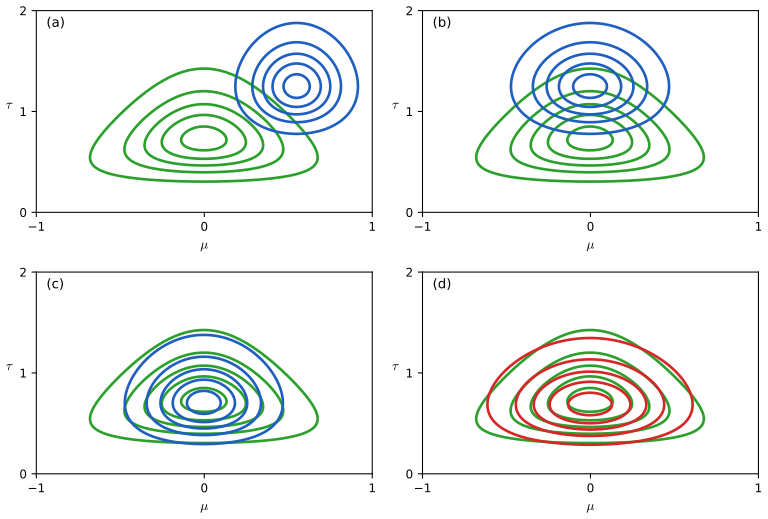
fig10_4. Download: PDF · SVGFor this model the fixed point can be found in closed form, and the comparison with the exact posterior is instructive.
Result 10.8 (the mean-field solution in closed form, and what it gets wrong)
Let \(C\)
The exact posterior is \(\N(\mu\given\mu_N,((\lambda_0+N)\tau)^{-1})\Gam(\tau\given a^\ast,b^\ast)\) with \(a^\ast=a_0+N/2\) and \(b^\ast=b_0+C/2\). Consequently:
- the means are exact: \(\E_q[\mu]\)
\({}=\E[\mu\given\mathcal{D}]\) \({}=\mu_N\) and \(\E_q[\tau]\) \({}=\E[\tau\given\mathcal{D}]\) \({}=a^\ast/b^\ast\); - \(\var_q[\tau]\)
\({}=\dfrac{a^\ast}{a^\ast+\frac12}\,\var[\tau\given\mathcal{D}]\); - \(\var_q[\mu]\)
\({}=\dfrac{a^\ast-1}{a^\ast}\,\var[\mu\given\mathcal{D}]\) (for \(a^\ast\gt1\)).
Both variances are too small, that of \(\mu\) the more so: the "too compact" effect of Result 10.5 again. The ratios tend to one as \(N\to\infty\).
Proof
Fixed point. Substitute \(\E[\tau]=a_N/b_N\) into \(b_N=b_0+\frac12(C+1/\E[\tau])\): \(b_N=b_0+\frac C2+\frac{b_N}{2a_N}\), so \(b_N(1-\frac1{2a_N})=b_0+\frac C2\) and \(b_N=\frac{(2b_0+C)\,a_N}{2a_N-1}\). With \(2a_N-1=2a_0+N\) this gives \(b_N\) and \(\E_q[\tau]\)
Exact posterior. Multiplying (10.21)–(10.23) and completing the square in \(\mu\) gives the Gaussian–Gamma posterior with \(a^\ast=a_0+N/2\) and \(b^\ast\)
(i) Hence \(\E_q[\tau]\)
(ii) \(\var_q[\tau]\)
(iii) \(\var_q[\mu]\)
I checked these formulas numerically against the iteration and against direct numerical integration of the exact posterior. With the non-informative choice below (\(a^\ast=N/2\)) and \(N=5\), \(q_\mu\) has only \(60\%\) of the posterior variance of \(\mu\); with \(N=100\), \(98\%\).
Non-informative priors. Take \(\mu_0=a_0=b_0=\lambda_0=0\). The priors are improper but the posterior is proper (for \(N\ge2\)). Then \(\mu_N=\bar x\), \(\lambda_N=N\E[\tau]\), \(a_N=\frac{N+1}{2}\), \(b_N\)
Filling the gap: solving for \(1/\E[\tau]\) p. 473, (10.33), Exercise 10.9
Derivation
Substitute (10.32) into (10.31): \(\overline{x^2}-2\bar x^2\)
Since \(1-\frac1{N+1}=\frac N{N+1}\),
\[ \frac{1}{\E[\tau]}=\overline{x^2}-\bar x^2=\frac1N\sum_{n=1}^{N}(x_n-\bar x)^2. \tag{10.33} \]This is also the special case \(a_0=b_0=\lambda_0=0\), \(C=Ns^2\) of Result 10.8. ∎
Erratum. Because of the missing \(\frac12\ln\tau\) (see (10.28)), the first printing has \(a_N=N/2\), the factor \(1/N\) instead of \(1/(N+1)\) in (10.31), and obtains \(1/\E[\tau]\)
1/N or 1/(N−1)?
The divisor is decided by the prior on \(\tau\), not by the factorisation, and in both cases mean field reproduces the exact posterior mean of \(\tau\) (Result 10.8(i)).
- With \(\lambda_0\to0\), the conditional prior (10.22) still contributes the factor \(\tau^{1/2}\) from its normaliser, so \(a_0=b_0=0\) means \(p(\mu,\tau)\propto\tau^{1/2}\cdot\tau^{-1}\)
\({}=\tau^{-1/2}\), the joint Jeffreys prior. Integrating \(\mu\) out of the exact posterior (\(\int e^{-N\tau(\mu-\bar x)^2/2}\d\mu\propto\tau^{-1/2}\)) gives \(p(\tau\given\mathcal{D})\) \({}=\Gam(\tau\given\frac N2,\frac{Ns^2}{2})\), so \(1/\E[\tau\given\mathcal{D}]=s^2\): divisor \(N\), as in the corrected (10.33). - With the reference prior \(p(\mu,\tau)\propto\tau^{-1}\) (flat in \(\mu\), \(1/\tau\) in \(\tau\)), \(p(\tau\given\mathcal{D})\)
\({}=\Gam(\tau\given\frac{N-1}2,\frac{Ns^2}2)\), so \(1/\E[\tau\given\mathcal{D}]\) \({}=\frac{N}{N-1}s^2\): divisor \(N-1\). Mean field with this prior has \(a_N=N/2\) and returns the same number. Dropping the \(\frac12\ln\tau\), as the first printing did, silently switches to this prior.
Neither quantity is "the" Bayesian estimate of the variance: under the first prior, for example, \(\E[\tau^{-1}\given\mathcal{D}]\)
10.1.4 Model comparison
Let \(m\) index candidate models with prior probabilities \(p(m)\). Different models can have different latent spaces, so \(q(\mathbf{Z})q(m)\) makes no sense; instead take \(q(\mathbf{Z},m)\)
Result 10.9 (variational posterior over models) p. 473 (10.36) Exercises 10.10 10.11
For fixed \(q(\mathbf{Z}\given m)\), define \(\LB_m\)
and the maximum is \(\LB\)
Proof
(10.34) is Result 10.1 applied to the pair \((\mathbf{Z},m)\) as the unobserved variables: \(p(\mathbf{Z},\mathbf{X},m)\)
with \(q^\star(m)\)
So the posterior over models is approximated by replacing each log evidence \(\ln p(\mathbf{X}\given m)\) with its lower bound \(\LB_m\). This is how the bounds of Figures 10.7 and 10.9 are used to choose the number of components and the polynomial degree.
Erratum. The first printing writes \(\LB_m\) for \(\LB\) in (10.34), (10.35) and the line between them, and does not define \(\LB_m\) after (10.36). The statements above follow the corrected text.
10.2 Illustration: variational mixture of Gaussians
The Gaussian mixture of Chapter 9 is the model on which variational Bayes is best understood (Attias 1999), and the book asks the reader to work through it in detail. Each \(\mathbf{x}_n\in\R^D\) has a one-of-\(K\) latent vector \(\mathbf{z}_n\); \(\mathbf{X}=\{\mathbf{x}_n\}\), \(\mathbf{Z}=\{\mathbf{z}_n\}\). Precision matrices \(\bm\Lambda_k\) are used instead of covariances because they simplify the algebra.
Definition 10.2 (the Bayesian Gaussian mixture) pp. 474–475, (10.37)–(10.40)
\[ p(\mathbf{Z}\given\bm\pi)=\prod_{n=1}^{N}\prod_{k=1}^{K}\pi_k^{z_{nk}} \tag{10.37} \] \[ p(\mathbf{X}\given\mathbf{Z},\bm\mu,\bm\Lambda)=\prod_{n=1}^{N}\prod_{k=1}^{K}\N\big(\mathbf{x}_n\given\bm\mu_k,\bm\Lambda_k^{-1}\big)^{z_{nk}} \tag{10.38} \] \[ p(\bm\pi)=\Dir(\bm\pi\given\bm\alpha_0)=C(\bm\alpha_0)\prod_{k=1}^{K}\pi_k^{\alpha_0-1} \tag{10.39} \] \[ p(\bm\mu,\bm\Lambda)=p(\bm\mu\given\bm\Lambda)p(\bm\Lambda)=\prod_{k=1}^{K}\N\big(\bm\mu_k\given\mathbf{m}_0,(\beta_0\bm\Lambda_k)^{-1}\big)\,\Wish(\bm\Lambda_k\given\mathbf{W}_0,\nu_0) \tag{10.40} \]Here \(C(\bm\alpha)\)
with the normaliser \(B(\mathbf{W},\nu)\) of (B.79) (toolkit: Dirichlet, Wishart). The hyperparameters are \(\alpha_0\) (a prior count per component), \(\mathbf{m}_0\) (usually \(\mathbf{0}\)), \(\beta_0\) (a prior count for the mean), \(\mathbf{W}_0\) and \(\nu_0\gt D-1\) (the prior guess of each precision is \(\E[\bm\Lambda_k]=\nu_0\mathbf{W}_0\)).
Both priors are conjugate, which is what will make every factor of the variational posterior a standard distribution. For \(\alpha_0\lt1\) the Dirichlet density is largest near the faces of the simplex (Figure 2.5), so the prior favours solutions with some \(\pi_k\) close to zero; this is the source of the pruning seen in Figure 10.6.
10.2.1 Variational distribution
The joint distribution of all the variables is
\[ p(\mathbf{X},\mathbf{Z},\bm\pi,\bm\mu,\bm\Lambda)=p(\mathbf{X}\given\mathbf{Z},\bm\mu,\bm\Lambda)\,p(\mathbf{Z}\given\bm\pi)\,p(\bm\pi)\,p(\bm\mu\given\bm\Lambda)\,p(\bm\Lambda), \tag{10.41} \]one factor per node of Figure 10.5, each conditioned on its parents. The only assumption we make is a split between latent variables and parameters:
\[ q(\mathbf{Z},\bm\pi,\bm\mu,\bm\Lambda)=q(\mathbf{Z})\,q(\bm\pi,\bm\mu,\bm\Lambda). \tag{10.42} \]All further structure (a factor per data point, a separate Dirichlet, a Gaussian–Wishart per component) will be derived. We drop the subscripts on \(q\) and let the arguments say which factor is meant.
Result 10.10 (the optimal factors of the variational mixture) pp. 476–479, (10.43)–(10.67)
Latent variables. With the soft counts, means and covariances
\[ N_k=\sum_{n=1}^{N}r_{nk} \tag{10.51} \] \[ \bar{\mathbf{x}}_k=\frac1{N_k}\sum_{n=1}^{N}r_{nk}\mathbf{x}_n \tag{10.52} \] \[ \mathbf{S}_k=\frac1{N_k}\sum_{n=1}^{N}r_{nk}(\mathbf{x}_n-\bar{\mathbf{x}}_k)(\mathbf{x}_n-\bar{\mathbf{x}}_k)^\T \tag{10.53} \]the update of \(q(\mathbf{Z})\) is \(q^\star(\mathbf{Z})\)
where \(\ln\tilde\pi_k\)
Parameters. The update of \(q(\bm\pi,\bm\mu,\bm\Lambda)\) factorises as \(q(\bm\pi)\prod_kq(\bm\mu_k,\bm\Lambda_k)\) (10.55), with \(q^\star(\bm\pi)\)
Note on (10.63)
Some printings, including the PDF used for these notes, print \(\nu_k=\nu_0+N_k+1\). The extra 1 is a misprint. The derivation below (count the powers of \(|\bm\Lambda_k|\)) gives \(\nu_0+N_k\), as does the official solution to Exercise 10.13 (Svensén and Bishop 2009), and the lower bound of Section 10.2.2 is stationary at \(\nu_0+N_k\) but not at \(\nu_0+N_k+1\) (Result 10.13; a finite-difference check on the Old Faithful data confirms both statements). The difference matters most for components with small \(N_k\).
Filling the gap: the factor \(q^\star(\mathbf{Z})\) pp. 476–477 (10.43)–(10.50) Exercise 10.12
Derivation
Step 1. By (10.9) with the factorisation (10.42),
\[ \ln q^\star(\mathbf{Z})=\E_{\bm\pi,\bm\mu,\bm\Lambda}[\ln p(\mathbf{X},\mathbf{Z},\bm\pi,\bm\mu,\bm\Lambda)]+\const. \tag{10.43} \]Step 2. Take logarithms in (10.41). The terms \(\ln p(\bm\pi)\), \(\ln p(\bm\mu\given\bm\Lambda)\), \(\ln p(\bm\Lambda)\) do not involve \(\mathbf{Z}\), so their expectations are constants:
\[ \ln q^\star(\mathbf{Z})=\E_{\bm\pi}[\ln p(\mathbf{Z}\given\bm\pi)]+\E_{\bm\mu,\bm\Lambda}[\ln p(\mathbf{X}\given\mathbf{Z},\bm\mu,\bm\Lambda)]+\const. \tag{10.44} \]Step 3. From (10.37) and (10.38), both logarithms are linear in the \(z_{nk}\), which are constants for the expectation over the parameters:
\[ \ln p(\mathbf{Z}\given\bm\pi)=\sum_{n,k}z_{nk}\ln\pi_k, \] \[ \ln p(\mathbf{X}\given\mathbf{Z},\bm\mu,\bm\Lambda)=\sum_{n,k}z_{nk}\Big\{\tfrac12\ln|\bm\Lambda_k|-\tfrac D2\ln2\pi-\tfrac12(\mathbf{x}_n-\bm\mu_k)^\T\bm\Lambda_k(\mathbf{x}_n-\bm\mu_k)\Big\}. \]Taking expectations term by term,
\[ \ln q^\star(\mathbf{Z})=\sum_{n=1}^{N}\sum_{k=1}^{K}z_{nk}\ln\rho_{nk}+\const \tag{10.45} \] \[ \begin{aligned}\ln\rho_{nk}&=\E[\ln\pi_k]+\frac12\E\big[\ln|\bm\Lambda_k|\big]-\frac D2\ln(2\pi)\\ &\quad-\frac12\E_{\bm\mu_k,\bm\Lambda_k}\big[(\mathbf{x}_n-\bm\mu_k)^\T\bm\Lambda_k(\mathbf{x}_n-\bm\mu_k)\big].\end{aligned} \tag{10.46} \]Step 4 (normalise). Exponentiating, \(q^\star(\mathbf{Z})\propto\prod_n\prod_k\rho_{nk}^{z_{nk}}\) (10.47). The normaliser is a sum over all \(K^N\) configurations, but the summand is a product of terms each depending on one \(\mathbf{z}_n\), so the sum factorises: \(\sum_{\mathbf{Z}}\prod_nf_n(\mathbf{z}_n)\)
Each \(\rho_{nk}\) is the exponential of a real number, so \(r_{nk}\gt0\) and \(\sum_kr_{nk}=1\). The posterior over \(\mathbf{Z}\) factorises over \(n\) even though we never assumed it (an induced factorisation, Section 10.2.5), and has the same form as the prior (10.37).
Step 5. Under (10.48), \(z_{nk}\) is a Bernoulli variable with \(q(z_{nk}=1)=r_{nk}\), so
\[ \E[z_{nk}]=r_{nk}. \tag{10.50} \]In code, compute \(\ln\rho_{nk}\) and then \(r_{nk}\)
Filling the gap: the factorisation (10.55) and \(q^\star(\bm\pi)\) pp. 477–478, (10.54)–(10.58)
Derivation
By (10.9), \(\ln q^\star(\bm\pi,\bm\mu,\bm\Lambda)\)
The right side has the form \(F(\bm\pi)+\sum_kG_k(\bm\mu_k,\bm\Lambda_k)\), with \(F\)
For \(\bm\pi\), use (10.39), (10.37) and (10.50):
\[ \begin{aligned}\ln q^\star(\bm\pi)&=(\alpha_0-1)\sum_{k=1}^{K}\ln\pi_k+\sum_{k=1}^{K}\sum_{n=1}^{N}r_{nk}\ln\pi_k+\const\\ &=\sum_{k=1}^{K}(\alpha_0+N_k-1)\ln\pi_k+\const.\end{aligned} \tag{10.56} \]On the simplex this is the logarithm of a Dirichlet kernel \(\prod_k\pi_k^{\alpha_k-1}\), so
\[ q^\star(\bm\pi)=\Dir(\bm\pi\given\bm\alpha) \tag{10.57} \] \[ \alpha_k=\alpha_0+N_k: \tag{10.58} \]the prior counts plus the soft counts, exactly the conjugate update with \(N_k\) in place of observed counts (toolkit: Dirichlet). ∎
Filling the gap: the Gaussian–Wishart factor (10.59)–(10.63) p. 478, Exercise 10.13
The book says the result is found "by inspecting (10.54)". Here is the inspection: first the conditional of \(\bm\mu_k\) given \(\bm\Lambda_k\) by completing the square, then the Wishart terms by subtraction.
Derivation
Drop the index \(k\) on \(\bm\mu,\bm\Lambda\) and write \(r_n=r_{nk}\). From \(G_k\) in Gap 10.7, using \(\ln\N(\bm\mu\given\mathbf{m}_0,(\beta_0\bm\Lambda)^{-1})\)
where \(\frac{N_k}2\ln|\bm\Lambda|\) came from \(\sum_nr_n\cdot\frac12\ln|\bm\Lambda|\).
Step 1: \(\bm\mu\) given \(\bm\Lambda\). The terms involving \(\bm\mu\) are
\[ -\tfrac12\bm\mu^\T(\beta_0+N_k)\bm\Lambda\bm\mu+\bm\mu^\T\bm\Lambda\Big(\beta_0\mathbf{m}_0+\sum_nr_n\mathbf{x}_n\Big)=-\tfrac12\bm\mu^\T(\beta_k\bm\Lambda)\bm\mu+\bm\mu^\T(\beta_k\bm\Lambda)\mathbf{m}_k, \]using \(\sum_nr_n\mathbf{x}_n\)
Step 2: the marginal of \(\bm\Lambda\). By the product rule \(\ln q^\star(\bm\Lambda)\)
\(\mathbf{M}\) does not depend on \(\bm\mu\): the terms \(\bm\mu\bm\mu^\T\) have total coefficient \(\beta_0+N_k-\beta_k=0\), and the terms linear in \(\bm\mu\) are \(-\bm\mu(\beta_0\mathbf{m}_0+N_k\bar{\mathbf{x}}_k)^\T\)
Splitting \(\mathbf{x}_n-\mathbf{m}_k\)
a Wishart density \(\Wish(\bm\Lambda\given\mathbf{W}_k,\nu_k)\): (10.62), (10.63), and with Step 1, (10.59). ∎
Filling the gap: the expectations (10.64)–(10.66) and the responsibilities (10.67) pp. 478–479, Exercise 10.14
Derivation
(10.64). Condition on \(\bm\Lambda_k\) first. Under \(\bm\mu_k\given\bm\Lambda_k\sim\N(\mathbf{m}_k,(\beta_k\bm\Lambda_k)^{-1})\), the expected quadratic form \(\E[\mathbf{y}^\T\mathbf{A}\mathbf{y}]\)
(10.65), (10.66). These are the standard log-moments of the Wishart and the Dirichlet (B.81), (B.21), proved in the toolkit (Wishart) and (Dirichlet):
\[ \ln\tilde\Lambda_k\equiv\E\big[\ln|\bm\Lambda_k|\big]=\sum_{i=1}^{D}\psi\Big(\frac{\nu_k+1-i}{2}\Big)+D\ln2+\ln|\mathbf{W}_k| \tag{10.65} \] \[ \ln\tilde\pi_k\equiv\E[\ln\pi_k]=\psi(\alpha_k)-\psi(\hat\alpha),\qquad \hat\alpha=\sum_k\alpha_k, \tag{10.66} \]with \(\psi\) the digamma function (B.25).
(10.67). Substitute into (10.46): \(\ln\rho_{nk}\)
Compare the maximum likelihood responsibilities (9.13), written with precisions,
\[ r_{nk}\propto\pi_k|\bm\Lambda_k|^{1/2}\exp\Big\{-\frac12(\mathbf{x}_n-\bm\mu_k)^\T\bm\Lambda_k(\mathbf{x}_n-\bm\mu_k)\Big\}. \tag{10.68} \]Point values are replaced by geometric means (\(\tilde\pi_k=e^{\E[\ln\pi_k]}\), \(\tilde\Lambda_k\)
Algorithm 10.3 (variational Bayes for the Gaussian mixture)
- Choose \(K\) and \(\alpha_0,\beta_0,\mathbf{m}_0,\mathbf{W}_0,\nu_0\). Initialise the responsibilities \(r_{nk}\) (from K-means or at random).
- Variational M step. Compute \(N_k,\bar{\mathbf{x}}_k,\mathbf{S}_k\) (10.51)–(10.53), then \(\alpha_k\) (10.58) and \(\beta_k,\mathbf{m}_k,\mathbf{W}_k,\nu_k\) (10.60)–(10.63), with \(\nu_k=\nu_0+N_k\).
- Variational E step. Compute \(\ln\tilde\pi_k\) (10.66), \(\ln\tilde\Lambda_k\) (10.65) and the expected quadratic forms (10.64); form \(\ln\rho_{nk}\) and normalise over \(k\) to get \(r_{nk}\) (10.67).
- Evaluate the bound \(\LB\) of Result 10.12. It never decreases; stop when its increase is below a tolerance.
The posterior mean of the mixing proportions is (Exercise 10.15; the Dirichlet mean \(\alpha_k/\hat\alpha\) with \(\hat\alpha\)
Erratum. The first printing has \(\alpha_k\) instead of \(\alpha_0\) in the numerator of (10.69).
Result 10.11 (why unneeded components switch off) pp. 479–480
Suppose component \(k\) has \(N_k\approx0\). Then \(\alpha_k\approx\alpha_0\), and by (10.60)–(10.63) \(\beta_k,\mathbf{m}_k,\mathbf{W}_k,\nu_k\) return to their prior values: the component reverts to the prior. In the next E step its responsibilities carry the factor
\[ \tilde\pi_k=e^{\psi(\alpha_0)-\psi(\hat\alpha)},\qquad \psi(\alpha_0)=-\frac{1}{\alpha_0}-\gamma+O(\alpha_0)\quad(\gamma=0.5772\ldots), \]whereas a component with \(N_j\) points has \(\tilde\pi_j\)
- \(\alpha_0=10^{-3}\): the ratio is about \(e^{-1000}\). The empty component can never win back a data point, \(N_k\) stays at zero, and \(\E[\pi_k]\)
\({}=\alpha_0/(K\alpha_0+N)\) \({}\approx0\) by (10.69): it has been switched off, permanently. - \(\alpha_0=1\): \(e^{\psi(1)}=e^{-\gamma}\approx0.56\), so the penalty is only a factor of order \(1/N_j\); an empty component can still collect points that the others fit badly (the book reports three surviving components on Old Faithful).
- \(\alpha_0\to\infty\): \(\E[\pi_k]\to1/K\) for every \(k\), and the prior keeps all components (all six survive for \(\alpha_0=10\)).
Proof
From \(\Gamma(x+1)=x\Gamma(x)\), \(\psi(x+1)=\psi(x)+1/x\), so \(\psi(\alpha_0)\)
This is the mechanical side of the "automatic trade-off between fitting the data and the complexity of the model" (Section 3.4). The statistical side is visible in the bound of Section 10.2.2, which can be rearranged as an expected log-likelihood minus \(\KL(q(\bm\pi)\|p(\bm\pi))\) and minus \(\sum_k\KL(q(\bm\mu_k,\bm\Lambda_k)\|p(\bm\mu_k,\bm\Lambda_k))\): a component pays a KL price for moving away from its prior, and a component that merely duplicates another improves the fit too little to pay it. Maximum likelihood has no such price, so EM with \(K=6\) keeps all six components.
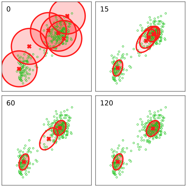
fig10_6. Download: PDF · SVGFilling the gap: for large \(N\) variational Bayes becomes EM p. 480, Exercise 10.20
The book states that as \(N\to\infty\) the Bayesian treatment "converges to the maximum likelihood EM algorithm". Here is why, for components with \(N_k\to\infty\) (\(N_k/N\) fixed).
Derivation
Parameters concentrate. \(\beta_k\sim N_k\), \(\nu_k\sim N_k\), \(\mathbf{m}_k\to\bar{\mathbf{x}}_k\) and \(\mathbf{W}_k^{-1}\sim N_k\mathbf{S}_k\) (the other terms of (10.62) are \(O(1)\)). So \(\E[\bm\Lambda_k]\)
Responsibilities. With \(\psi(x)=\ln x+O(1/x)\) (10.241), \(\ln\tilde\pi_k\)
Predictive density. In (10.81) below, \(\alpha_k/\hat\alpha\to N_k/N\) and the Student densities, with degrees of freedom \(\nu_k+1-D\to\infty\), become Gaussians \(\N(\hat{\mathbf{x}}\given\bar{\mathbf{x}}_k,\mathbf{S}_k)\): a mixture of Gaussians with the maximum likelihood parameters. ∎
Three practical advantages over maximum likelihood come at almost no extra cost (the dominant work, the responsibilities and the weighted covariances, is the same as in EM). The singularities of Section 9.2.1, where a component collapses onto one data point, are absent: \(\mathbf{W}_k^{-1}\succeq\mathbf{W}_0^{-1}\) keeps every precision bounded (they are absent from MAP estimation too, Exercise 10.24). Large \(K\) does not over-fit (Figure 10.6). And the bound can be used to choose \(K\) (Section 10.2.4).
10.2.2 Variational lower bound
Monitoring \(\LB\) is the best test of both the algebra and the code: it must not decrease at any step, and finite differences can check that each update maximises it (Svensén and Bishop 2005). For the mixture,
\[ \begin{aligned}\LB&=\sum_{\mathbf{Z}}\iiint q(\mathbf{Z},\bm\pi,\bm\mu,\bm\Lambda)\ln\left\{\frac{p(\mathbf{X},\mathbf{Z},\bm\pi,\bm\mu,\bm\Lambda)}{q(\mathbf{Z},\bm\pi,\bm\mu,\bm\Lambda)}\right\}\d\bm\pi\,\d\bm\mu\,\d\bm\Lambda\\ &=\E[\ln p(\mathbf{X}\given\mathbf{Z},\bm\mu,\bm\Lambda)]+\E[\ln p(\mathbf{Z}\given\bm\pi)]+\E[\ln p(\bm\pi)]+\E[\ln p(\bm\mu,\bm\Lambda)]\\ &\quad-\E[\ln q(\mathbf{Z})]-\E[\ln q(\bm\pi)]-\E[\ln q(\bm\mu,\bm\Lambda)]\end{aligned} \tag{10.70} \]where each expectation is over all the variables in its argument, under the current \(q\).
Result 10.12 (the terms of the bound) pp. 481–482 (10.71)–(10.77) Exercises 10.16 10.17
\[ \begin{aligned}\E[\ln p(\mathbf{X}\given\mathbf{Z},\bm\mu,\bm\Lambda)]=\frac12\sum_{k=1}^{K}N_k\Big\{&\ln\tilde\Lambda_k-D\beta_k^{-1}-\nu_k\Tr(\mathbf{S}_k\mathbf{W}_k)\\ &-\nu_k(\bar{\mathbf{x}}_k-\mathbf{m}_k)^\T\mathbf{W}_k(\bar{\mathbf{x}}_k-\mathbf{m}_k)-D\ln(2\pi)\Big\}\end{aligned} \tag{10.71} \] \[ \E[\ln p(\mathbf{Z}\given\bm\pi)]=\sum_{n=1}^{N}\sum_{k=1}^{K}r_{nk}\ln\tilde\pi_k \tag{10.72} \] \[ \E[\ln p(\bm\pi)]=\ln C(\bm\alpha_0)+(\alpha_0-1)\sum_{k=1}^{K}\ln\tilde\pi_k \tag{10.73} \] \[ \begin{aligned}\E[\ln p(\bm\mu,\bm\Lambda)]&=\frac12\sum_{k=1}^{K}\Big\{D\ln(\beta_0/2\pi)+\ln\tilde\Lambda_k-\frac{D\beta_0}{\beta_k}\\ &\qquad\qquad-\beta_0\nu_k(\mathbf{m}_k-\mathbf{m}_0)^\T\mathbf{W}_k(\mathbf{m}_k-\mathbf{m}_0)\Big\}\\ &\quad+K\ln B(\mathbf{W}_0,\nu_0)+\frac{\nu_0-D-1}{2}\sum_{k=1}^{K}\ln\tilde\Lambda_k-\frac12\sum_{k=1}^{K}\nu_k\Tr(\mathbf{W}_0^{-1}\mathbf{W}_k)\end{aligned} \tag{10.74} \] \[ \E[\ln q(\mathbf{Z})]=\sum_{n=1}^{N}\sum_{k=1}^{K}r_{nk}\ln r_{nk} \tag{10.75} \] \[ \E[\ln q(\bm\pi)]=\sum_{k=1}^{K}(\alpha_k-1)\ln\tilde\pi_k+\ln C(\bm\alpha) \tag{10.76} \] \[ \E[\ln q(\bm\mu,\bm\Lambda)]=\sum_{k=1}^{K}\Big\{\frac12\ln\tilde\Lambda_k+\frac D2\ln\Big(\frac{\beta_k}{2\pi}\Big)-\frac D2-\mathrm{H}[q(\bm\Lambda_k)]\Big\} \tag{10.77} \]with the Wishart entropy \(\mathrm{H}[q(\bm\Lambda_k)]\)
Filling the gap: deriving every term p. 481, "easily evaluated"
Two facts are used throughout: \(q(\mathbf{Z})\) and \(q(\bm\mu,\bm\Lambda)\) are independent, so \(\E[z_{nk}f(\bm\mu_k,\bm\Lambda_k)]\)
proved by writing \(\mathbf{x}_n-\mathbf{m}\)
Derivation
(10.71). By (10.64), (10.65),
\[ \begin{aligned}\E[\ln p(\mathbf{X}\given\mathbf{Z},\bm\mu,\bm\Lambda)]&=\sum_{n,k}r_{nk}\E[\ln\N(\mathbf{x}_n\given\bm\mu_k,\bm\Lambda_k^{-1})]\\ &=\frac12\sum_{n,k}r_{nk}\big\{\ln\tilde\Lambda_k-D\ln2\pi-D\beta_k^{-1}-\nu_k(\mathbf{x}_n-\mathbf{m}_k)^\T\mathbf{W}_k(\mathbf{x}_n-\mathbf{m}_k)\big\}.\end{aligned} \]Sum over \(n\) with the identity above (\(\mathbf{A}=\mathbf{W}_k\), \(\mathbf{m}=\mathbf{m}_k\)) and \(\sum_nr_{nk}=N_k\).
(10.72). \(\ln p(\mathbf{Z}\given\bm\pi)\)
(10.73). \(\ln\Dir(\bm\pi\given\bm\alpha_0)\)
(10.74). For each \(k\), \(\E[\ln\N(\bm\mu_k\given\mathbf{m}_0,(\beta_0\bm\Lambda_k)^{-1})]\)
(10.75). \(\ln q(\mathbf{Z})\)
(10.76). \(\ln\Dir(\bm\pi\given\bm\alpha)\)
(10.77). \(\ln q(\bm\mu_k,\bm\Lambda_k)\)
Checks. I verified each term against Monte Carlo averages under \(q\) (3000 draws, Old Faithful, \(K=6\)): agreement to Monte Carlo error. Summing the terms, the total coefficient of \(\ln\tilde\Lambda_k\) is \(\frac{N_k}2+\frac12\)
Result 10.13 (the updates maximise the bound) p. 482, Exercise 10.18
(a) General principle. Let \(q_j(\mathbf{z})\)
so \(\bm\eta=\tilde{\bm\eta}\) is the only stationary point. (b) For the mixture, the bound (10.70)–(10.77) written as a function of \(r_{nk},\alpha_k,\beta_k,\mathbf{m}_k,\mathbf{W}_k,\nu_k\) is stationary exactly at (10.49), (10.58), (10.60)–(10.62) and \(\nu_k=\nu_0+N_k\).
Proof
(a) By (10.6), \(\LB\)
(b) The explicit derivatives, from Result 10.12:
Responsibilities. (10.71) and (10.72) together equal \(\sum_{n,k}r_{nk}\ln\rho_{nk}\) with \(\ln\rho_{nk}\) of (10.46) (expand \(N_k,\bar{\mathbf{x}}_k,\mathbf{S}_k\) back into sums over \(n\)), and (10.75) contributes \(-\sum_{n,k}r_{nk}\ln r_{nk}\). With a multiplier \(\lambda_n\) for \(\sum_kr_{nk}=1\): \(\ln\rho_{nk}-\ln r_{nk}-1+\lambda_n\)
Dirichlet. The terms with \(\bm\alpha\) are \(\sum_k(\alpha_0+N_k-\alpha_k)\ln\tilde\pi_k\)
Means. The terms with \(\mathbf{m}_k\) are \(-\frac{\nu_k}2\{N_k(\bar{\mathbf{x}}_k-\mathbf{m}_k)^\T\mathbf{W}_k(\bar{\mathbf{x}}_k-\mathbf{m}_k)\)
\(\beta_k\). The terms are \(-\frac{D(N_k+\beta_0)}{2\beta_k}\)
Wishart parameters. Collecting the terms with \(\mathbf{W}=\mathbf{W}_k\), \(\nu=\nu_k\) (the coefficient of \(\ln\tilde\Lambda_k\) was found in Gap 10.11):
\[ f(\mathbf{W},\nu)=\frac{\nu_0+N_k-\nu}{2}\ln\tilde\Lambda(\mathbf{W},\nu)-\frac\nu2\Tr(\mathbf{W}\mathbf{M}_k)-\ln B(\mathbf{W},\nu)+\frac{\nu D}{2}, \]with \(\mathbf{M}_k\)
The first vanishes iff \(\mathbf{W}\)
So the bound offers a second route to the update equations: fix the functional forms that conjugacy guarantees (discrete, Dirichlet, Gaussian–Wishart), write \(\LB\) as a function of their parameters and maximise. In code, the finite-difference version of this check catches most errors.
10.2.3 Predictive density
For a new point \(\hat{\mathbf{x}}\) with latent \(\hat{\mathbf{z}}\),
\[ p(\hat{\mathbf{x}}\given\mathbf{X})=\sum_{\hat{\mathbf{z}}}\iiint p(\hat{\mathbf{x}}\given\hat{\mathbf{z}},\bm\mu,\bm\Lambda)\,p(\hat{\mathbf{z}}\given\bm\pi)\,p(\bm\pi,\bm\mu,\bm\Lambda\given\mathbf{X})\,\d\bm\pi\,\d\bm\mu\,\d\bm\Lambda. \tag{10.78} \]Summing over the \(K\) values of \(\hat{\mathbf{z}}\) (the summand is \(\prod_k[\pi_k\N(\hat{\mathbf{x}}\given\bm\mu_k,\bm\Lambda_k^{-1})]^{\hat z_k}\)),
\[ p(\hat{\mathbf{x}}\given\mathbf{X})=\sum_{k=1}^{K}\iiint\pi_k\,\N\big(\hat{\mathbf{x}}\given\bm\mu_k,\bm\Lambda_k^{-1}\big)\,p(\bm\pi,\bm\mu,\bm\Lambda\given\mathbf{X})\,\d\bm\pi\,\d\bm\mu\,\d\bm\Lambda \tag{10.79} \]and replacing the unknown posterior by \(q(\bm\pi)\prod_jq(\bm\mu_j,\bm\Lambda_j)\), in each term the factors \(j\ne k\) integrate to one:
\[ p(\hat{\mathbf{x}}\given\mathbf{X})\simeq\sum_{k=1}^{K}\iiint\pi_k\,\N\big(\hat{\mathbf{x}}\given\bm\mu_k,\bm\Lambda_k^{-1}\big)\,q(\bm\pi)\,q(\bm\mu_k,\bm\Lambda_k)\,\d\bm\pi\,\d\bm\mu_k\,\d\bm\Lambda_k. \tag{10.80} \]Erratum. The first printing has "=" instead of "\(\simeq\)" in (10.80) and (10.81).
Result 10.14 (a mixture of Student t densities) p. 483 (10.81)–(10.82) Exercise 10.19
\[ p(\hat{\mathbf{x}}\given\mathbf{X})\simeq\frac1{\hat\alpha}\sum_{k=1}^{K}\alpha_k\,\St\big(\hat{\mathbf{x}}\given\mathbf{m}_k,\mathbf{L}_k,\nu_k+1-D\big) \tag{10.81} \] \[ \mathbf{L}_k=\frac{(\nu_k+1-D)\beta_k}{1+\beta_k}\mathbf{W}_k. \tag{10.82} \]The \(k\)th component has mean \(\mathbf{m}_k\) and precision matrix \(\mathbf{L}_k\). As \(N\to\infty\) it becomes the mixture of Gaussians with the maximum likelihood parameters (Gap 10.10).
Filling the gap: the three integrals in (10.80) p. 483
Derivation
Over \(\bm\pi\). \(\int\pi_kq(\bm\pi)\,\d\bm\pi\)
Over \(\bm\mu_k\). Given \(\bm\Lambda_k=\bm\Lambda\), \(\hat{\mathbf{x}}\)
Over \(\bm\Lambda_k\). Drop \(k\) and put \(\bm\delta\)
with \(\mathbf{W}'^{-1}\)
By the matrix determinant lemma \(|\mathbf{W}^{-1}+c\bm\delta\bm\delta^\T|\)
Compare the Student density \(\St(\hat{\mathbf{x}}\given\mathbf{m},\mathbf{L},\nu')\)
10.2.4 Determining the number of components
For generic parameter values, relabelling the components (a permutation \(\sigma\) of \(\{1,\dots,K\}\) applied to \((\pi_k,\bm\mu_k,\bm\Lambda_k)\) and to the coordinates of every \(\mathbf{z}_n\)) leaves \(p(\mathbf{X})\) and the prior unchanged; there are \(K!\) such permutations, all giving different parameter vectors (Exercise 10.21). So every mode of the posterior comes with \(K!-1\) equivalent copies. Maximum likelihood does not care, since EM finds one of them. A variational \(q\) minimising \(\KL(q\|p)\) also sits on one copy (Figure 10.3, not Figure 10.2 as in the first printing), which is harmless for prediction with a fixed \(K\), but the bound then misses most of the posterior mass, and the amount it misses depends on \(K\).
Result 10.15 (the \(\ln K!\) correction) p. 484, Exercise 10.22
Let \(q\) be concentrated near one mode and let \(q_{\rm mix}\)
So when comparing different \(K\), add \(\ln K!\) to the bound of a single-mode solution.
Proof
Write \(\bm\theta\) for all unobserved variables (\(\mathbf{Z}\) and the parameters). \(\LB(q_{\rm mix})\)
Figure 10.7 shows the corrected bound against \(K\) for the Old Faithful data: a clear peak at \(K=2\), whereas the maximised likelihood keeps increasing with \(K\) and cannot choose the model (Section 3.4). Two cautions. First (Exercise 10.25), the factorised \(q\) under-estimates the posterior spread (Section 10.1.2), so \(\LB\) under-estimates \(\ln p(\mathbf{X}\given K)\), and the shortfall tends to grow with the number of parameters: this biases the comparison towards fewer components. Second, the \(\ln K!\) correction assumes that the \(K!\) copies do not overlap; when some components coincide (for example several switched-off components all sitting at the prior) there are fewer distinct copies, and adding \(\ln K!\) over-states the bound for large \(K\).
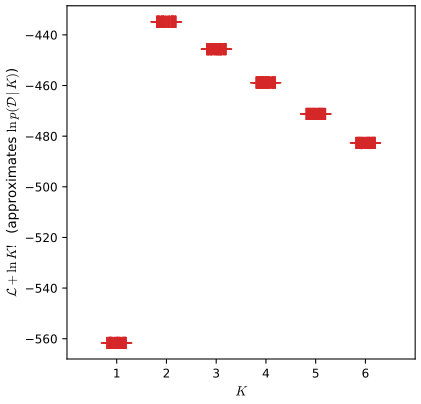
fig10_7. Download: PDF · SVGPoint estimates of \(\bm\pi\). Instead of comparing several \(K\), one can drop the prior on \(\bm\pi\), treat \(\bm\pi\) as a parameter and maximise \(\LB\) over it (Corduneanu and Bishop 2001). Only (10.72), now \(\sum_{n,k}r_{nk}\ln\pi_k\), depends on \(\bm\pi\); maximising with a multiplier for \(\sum_k\pi_k=1\), exactly as for (9.22), gives (Exercise 10.23)
\[ \pi_k=\frac1N\sum_{n=1}^{N}r_{nk}, \tag{10.83} \]interleaved with the variational updates of the other factors. Components that explain too little have \(\pi_k\) driven to zero and drop out: a single run from a generous \(K\) prunes itself, by the same automatic relevance determination mechanism as in the relevance vector machine (Section 7.2.2).
10.2.5 Induced factorisations
We assumed only (10.42), yet \(q^\star\) factorised further: over \(n\) in \(q(\mathbf{Z})\) and into \(q(\bm\pi)\prod_kq(\bm\mu_k,\bm\Lambda_k)\). (Not over \(k\) within \(\mathbf{z}_n\): its components are tied by \(\sum_kz_{nk}=1\).) These induced factorisations come from the conditional independences of the true model, and an implementation should exploit them, for example by never storing a full precision matrix for a Gaussian that is known to factorise. Partition the latent variables into \(\mathbf{A},\mathbf{B},\mathbf{C}\) and assume
\[ q(\mathbf{A},\mathbf{B},\mathbf{C})=q(\mathbf{A},\mathbf{B})\,q(\mathbf{C}). \tag{10.84} \]Result 10.16 (a test for induced factorisations) pp. 485–486, (10.85)–(10.86)
\[ \ln q^\star(\mathbf{A},\mathbf{B})=\E_{\mathbf{C}}[\ln p(\mathbf{X},\mathbf{A},\mathbf{B},\mathbf{C})]+\const=\E_{\mathbf{C}}[\ln p(\mathbf{A},\mathbf{B}\given\mathbf{X},\mathbf{C})]+\const. \tag{10.85} \]If
\[ \mathbf{A}\perp\!\!\!\perp\mathbf{B}\given\mathbf{X},\mathbf{C} \tag{10.86} \]then \(q^\star(\mathbf{A},\mathbf{B})\)
Proof
(10.85) is (10.9) followed by the product rule \(\ln p(\mathbf{X},\mathbf{A},\mathbf{B},\mathbf{C})\)
The mixture. With \(\mathbf{C}=\mathbf{Z}\), every path from \(\bm\pi\) to \(\bm\mu\) or \(\bm\Lambda\) in Figure 10.5 passes through some \(\mathbf{z}_n\) as \(\bm\pi\)
but the graph cannot show it, since \(\mathbf{x}_n\) has every \(\bm\mu_k\) as a parent and conditioning on it couples them. The independence holds for each value of \(\mathbf{Z}\) separately ("context-specific" independence). d-separation is a sufficient test, not a necessary one.
10.3 Variational linear regression
In the evidence framework of Section 3.5 the hyperparameters of Bayesian linear regression were fixed at the values maximising the marginal likelihood. A fully Bayesian treatment integrates over them; exact integration is intractable, but a variational approximation is easy. Keep the noise precision \(\beta\) fixed at its true value (Exercise 10.26 adds a Gamma prior on \(\beta\)) and put a Gamma prior on the weight precision \(\alpha\). With \(\bm\phi_n\)
The graph (Figure 10.8) is the chain \(\alpha\to\mathbf{w}\to t_n\), with the inputs \(\bm\phi_n\) and \(\beta\) as fixed quantities. This example is simple, but it sets up the variational logistic regression of Section 10.6.
10.3.1 Variational distribution
Take \(q(\mathbf{w},\alpha)\)
Result 10.17 (the two factors) pp. 487–488, (10.92)–(10.103)
\[ q^\star(\alpha)=\Gam(\alpha\given a_N,b_N) \tag{10.93} \] \[ a_N=a_0+\frac M2 \tag{10.94} \] \[ b_N=b_0+\frac12\E[\mathbf{w}^\T\mathbf{w}] \tag{10.95} \] \[ q^\star(\mathbf{w})=\N(\mathbf{w}\given\mathbf{m}_N,\mathbf{S}_N) \tag{10.99} \] \[ \mathbf{m}_N=\beta\mathbf{S}_N\bm\Phi^\T\mathbf{t} \tag{10.100} \] \[ \mathbf{S}_N=\big(\E[\alpha]\mathbf{I}+\beta\bm\Phi^\T\bm\Phi\big)^{-1} \tag{10.101} \]with the moments
\[ \E[\alpha]=a_N/b_N \tag{10.102} \] \[ \E[\mathbf{w}\mathbf{w}^\T]=\mathbf{m}_N\mathbf{m}_N^\T+\mathbf{S}_N, \tag{10.103} \]so that \(\E[\mathbf{w}^\T\mathbf{w}]\)
\(q(\mathbf{w})\) is the fixed-\(\alpha\) posterior (3.52) with \(\alpha\) replaced by \(\E[\alpha]\).
Filling the gap: the factors (10.92)–(10.101) pp. 487–488
Derivation
The factor \(q(\alpha)\). By (10.9), only the factors of (10.90) that involve \(\alpha\) matter: \(\ln q^\star(\alpha)\)
This is \((a_N-1)\ln\alpha-b_N\alpha\): the logarithm of \(\Gam(\alpha\given a_N,b_N)\) with (10.94) and (10.95).
The factor \(q(\mathbf{w})\). Now \(\ln p(\alpha)\) is constant:
\[ \ln q^\star(\mathbf{w})=\ln p(\mathbf{t}\given\mathbf{w})+\E_\alpha[\ln p(\mathbf{w}\given\alpha)]+\const \tag{10.96} \] \[ =-\frac\beta2\sum_{n=1}^{N}\{\mathbf{w}^\T\bm\phi_n-t_n\}^2-\frac12\E[\alpha]\,\mathbf{w}^\T\mathbf{w}+\const \tag{10.97} \] \[ =-\frac12\mathbf{w}^\T\big(\E[\alpha]\mathbf{I}+\beta\bm\Phi^\T\bm\Phi\big)\mathbf{w}+\beta\mathbf{w}^\T\bm\Phi^\T\mathbf{t}+\const, \tag{10.98} \]expanding the square and using \(\sum_n\bm\phi_n\bm\phi_n^\T\)
Moments. (10.102) is the Gamma mean (B.27) and (10.103) the Gaussian second moment (toolkit: Gaussian facts); \(\E[\mathbf{w}^\T\mathbf{w}]\)
Algorithm 10.4 (variational linear regression)
- Set \(a_N=a_0+M/2\) once. Initialise \(\E[\alpha]\).
- Update \(q(\mathbf{w})\): \(\mathbf{S}_N\)
\({}=(\E[\alpha]\mathbf{I}+\beta\bm\Phi^\T\bm\Phi)^{-1}\), \(\mathbf{m}_N\) \({}=\beta\mathbf{S}_N\bm\Phi^\T\mathbf{t}\). - Update \(q(\alpha)\): \(b_N\)
\({}=b_0+\frac12(\mathbf{m}_N^\T\mathbf{m}_N+\Tr\mathbf{S}_N)\), \(\E[\alpha]=a_N/b_N\). - Evaluate \(\LB\) (Result 10.18) and repeat 2–4 until it stops increasing.
Relation to the evidence framework. With \(a_0=b_0=0\) (an infinitely broad prior),
\[ \E[\alpha]=\frac{a_N}{b_N}=\frac{M/2}{\E[\mathbf{w}^\T\mathbf{w}]/2}=\frac{M}{\mathbf{m}_N^\T\mathbf{m}_N+\Tr(\mathbf{S}_N)}. \tag{10.104} \]This is the EM re-estimate (9.63) of \(\alpha\) for the evidence (Section 9.3.4), with the point estimate replaced by \(\E[\alpha]\). Because \(q(\mathbf{w})\) depends on \(q(\alpha)\) only through \(\E[\alpha]\), the variational iteration and the EM iteration are the same map, so they converge to the same \(\mathbf{m}_N,\mathbf{S}_N\), with \(\E[\alpha]\) equal to the evidence maximiser. The variational approach adds a whole distribution for \(\alpha\), \(\Gam(M/2,b_N)\), whose coefficient of variation \(\sqrt{2/M}\) shows how poorly \(\alpha\) is determined when there are few weights.
10.3.2 Predictive distribution
\[ \begin{aligned}p(t\given\mathbf{x},\mathbf{t})&=\int p(t\given\mathbf{x},\mathbf{w})p(\mathbf{w}\given\mathbf{t})\,\d\mathbf{w}\\ &\simeq\int\N(t\given\mathbf{w}^\T\bm\phi(\mathbf{x}),\beta^{-1})\N(\mathbf{w}\given\mathbf{m}_N,\mathbf{S}_N)\,\d\mathbf{w}\\ &=\N\big(t\given\mathbf{m}_N^\T\bm\phi(\mathbf{x}),\sigma^2(\mathbf{x})\big)\end{aligned} \tag{10.105} \] \[ \sigma^2(\mathbf{x})=\frac1\beta+\bm\phi(\mathbf{x})^\T\mathbf{S}_N\bm\phi(\mathbf{x}). \tag{10.106} \]Filling the gap: the predictive integral p. 488, (10.105)–(10.106)
Derivation
Under \(q\), \(t=\bm\phi^\T\mathbf{w}+\epsilon\) with \(\mathbf{w}\sim\N(\mathbf{m}_N,\mathbf{S}_N)\) and independent \(\epsilon\sim\N(0,\beta^{-1})\): a linear-Gaussian model (2.115) with \(\mathbf{A}=\bm\phi^\T\) (toolkit). A linear function of a Gaussian plus independent Gaussian noise is Gaussian with mean \(\bm\phi^\T\mathbf{m}_N\) and variance \(\bm\phi^\T\mathbf{S}_N\bm\phi+\beta^{-1}\). The second term is the uncertainty about \(\mathbf{w}\); it is the same as (3.59) with \(\E[\alpha]\) inside \(\mathbf{S}_N\). ∎
10.3.3 Lower bound
\[ \begin{aligned}\LB(q)&=\E[\ln p(\mathbf{w},\alpha,\mathbf{t})]-\E[\ln q(\mathbf{w},\alpha)]\\ &=\E_{\mathbf{w}}[\ln p(\mathbf{t}\given\mathbf{w})]+\E_{\mathbf{w},\alpha}[\ln p(\mathbf{w}\given\alpha)]+\E_\alpha[\ln p(\alpha)]-\E_{\mathbf{w}}[\ln q(\mathbf{w})]-\E_\alpha[\ln q(\alpha)].\end{aligned} \tag{10.107} \]Result 10.18 (the bound for variational linear regression) p. 489 (10.108)–(10.112) Exercise 10.27
\[ \E[\ln p(\mathbf{t}\given\mathbf{w})]_{\mathbf{w}}=\frac N2\ln\Big(\frac{\beta}{2\pi}\Big)-\frac\beta2\mathbf{t}^\T\mathbf{t}+\beta\mathbf{m}_N^\T\bm\Phi^\T\mathbf{t}-\frac\beta2\Tr\big[\bm\Phi^\T\bm\Phi(\mathbf{m}_N\mathbf{m}_N^\T+\mathbf{S}_N)\big] \tag{10.108} \] \[ \begin{aligned}\E[\ln p(\mathbf{w}\given\alpha)]_{\mathbf{w},\alpha}&=-\frac M2\ln(2\pi)+\frac M2\big(\psi(a_N)-\ln b_N\big)\\ &\quad-\frac{a_N}{2b_N}\big[\mathbf{m}_N^\T\mathbf{m}_N+\Tr(\mathbf{S}_N)\big]\end{aligned} \tag{10.109} \] \[ \E[\ln p(\alpha)]_\alpha=a_0\ln b_0+(a_0-1)\big[\psi(a_N)-\ln b_N\big]-b_0\frac{a_N}{b_N}-\ln\Gamma(a_0) \tag{10.110} \] \[ -\E[\ln q(\mathbf{w})]_{\mathbf{w}}=\frac12\ln|\mathbf{S}_N|+\frac M2\big[1+\ln(2\pi)\big] \tag{10.111} \] \[ -\E[\ln q(\alpha)]_\alpha=\ln\Gamma(a_N)-(a_N-1)\psi(a_N)-\ln b_N+a_N. \tag{10.112} \]Erratum. The first printing has \(\ln\Gamma(a_N)\) as the last term of (10.110); it should be \(\ln\Gamma(a_0)\) (the normaliser of the prior). The last term of (10.107) is written "\(-\E_\alpha[\ln q(\mathbf{w})]_{\mathbf{w}}\)" in the book; it is \(-\E_{\mathbf{w}}[\ln q(\mathbf{w})]\).
Filling the gap: the five terms p. 489, "straightforward"
Derivation
(10.108). \(\ln p(\mathbf{t}\given\mathbf{w})\)
(10.109). \(\ln p(\mathbf{w}\given\alpha)\)
(10.110). \(\ln\Gam(\alpha\given a_0,b_0)\)
(10.111). The entropy of \(\N(\mathbf{m}_N,\mathbf{S}_N)\) in \(M\) dimensions is \(\frac12\ln|\mathbf{S}_N|\)
(10.112). The entropy of \(\Gam(a_N,b_N)\) (B.31): \(-\E[\ln\Gam]\)
A Monte Carlo check of all five terms on a small polynomial problem agrees to sampling error.
Figure 10.9 plots \(\LB\) against the polynomial order for ten points from a cubic. By Section 10.1.4, with equal prior probabilities for the models, \(q(M)\propto e^{\LB_M}\): the bound acts as an approximate log evidence \(\ln p(\mathbf{t}\given M)\), and it peaks at the true order, whereas the training error keeps decreasing with the order. The figure uses \(a_0=b_0=0\), the prior \(p(\alpha)\propto1/\alpha\) (uniform in \(\ln\alpha\)). Then the term \(-\ln\Gamma(a_0)\) of (10.110) is infinite, but it is the same for every model, so differences of \(\LB\) between models, which are all that model comparison uses, are finite; in practice it is dropped (or \(a_0=b_0\) is set to a tiny positive number).
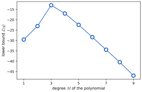
fig10_9. Download: PDF · SVGErratum. On p. 489, line −7, "\(p(\mathbf{t}\given M)\)" should be "\(\ln p(\mathbf{t}\given M)\)".
10.4 Exponential family distributions
In many models the complete-data likelihood \(p(\mathbf{X},\mathbf{Z}\given\bm\eta)\) is in the exponential family even though the marginal likelihood is not (a Gaussian mixture is not an exponential family, but the joint of \(\mathbf{x}_n\) and its label \(\mathbf{z}_n\) is). Distinguish latent variables \(\mathbf{Z}\), which are extensive (one per data point), from parameters \(\bm\eta\), which are intensive (fixed in number). For iid data,
\[ p(\mathbf{X},\mathbf{Z}\given\bm\eta)=\prod_{n=1}^{N}h(\mathbf{x}_n,\mathbf{z}_n)\,g(\bm\eta)\exp\big\{\bm\eta^\T\mathbf{u}(\mathbf{x}_n,\mathbf{z}_n)\big\} \tag{10.113} \]with the conjugate prior, interpretable as \(\nu_0\) pseudo-observations whose sufficient statistic has average \(\bm\chi_0\),
\[ p(\bm\eta\given\nu_0,\bm\chi_0)=f(\nu_0,\bm\chi_0)\,g(\bm\eta)^{\nu_0}\exp\big\{\nu_0\bm\eta^\T\bm\chi_0\big\}. \tag{10.114} \]Erratum. The first printing has \(p(\bm\eta\given\nu_0,\mathbf{v}_0)\) on the left of (10.114), and omits the factors \(\nu_0\) and \(\nu_N\) in front of \(\bm\eta^\T\bm\chi_0\) in (10.118) and \(\bm\eta^\T\bm\chi_N\) in (10.119), and on the left of (10.121). The corrected forms are used below.
Result 10.19 (variational Bayes for conjugate exponential families) pp. 490–491, (10.115)–(10.121)
With \(q(\mathbf{Z},\bm\eta)\)
and
\[ q^\star(\bm\eta)=f(\nu_N,\bm\chi_N)\,g(\bm\eta)^{\nu_N}\exp\big\{\nu_N\bm\eta^\T\bm\chi_N\big\} \tag{10.119} \] \[ \nu_N=\nu_0+N \tag{10.120} \] \[ \nu_N\bm\chi_N=\nu_0\bm\chi_0+\sum_{n=1}^{N}\E_{\mathbf{z}_n}[\mathbf{u}(\mathbf{x}_n,\mathbf{z}_n)]. \tag{10.121} \]The parameter update is the exact conjugate update with the unobserved sufficient statistics replaced by their expectations.
Filling the gap: the two factors, and the normaliser in (10.116) p. 491
Derivation
Latent variables. By (10.9), and since \(\ln g(\bm\eta)\) does not involve \(\mathbf{Z}\),
\[ \begin{aligned}\ln q^\star(\mathbf{Z})&=\E_{\bm\eta}[\ln p(\mathbf{X},\mathbf{Z}\given\bm\eta)]+\const\\ &=\sum_{n=1}^{N}\big\{\ln h(\mathbf{x}_n,\mathbf{z}_n)+\E[\bm\eta^\T]\mathbf{u}(\mathbf{x}_n,\mathbf{z}_n)\big\}+\const.\end{aligned} \tag{10.115} \](The prior \(\ln p(\bm\eta)\) is also constant in \(\mathbf{Z}\).) A sum over \(n\) of functions of \(\mathbf{z}_n\) exponentiates to a product, so \(q^\star(\mathbf{Z})\)
Parameters. By (10.9),
\[ \ln q^\star(\bm\eta)=\ln p(\bm\eta\given\nu_0,\bm\chi_0)+\E_{\mathbf{Z}}[\ln p(\mathbf{X},\mathbf{Z}\given\bm\eta)]+\const \tag{10.117} \] \[ =\nu_0\ln g(\bm\eta)+\nu_0\bm\eta^\T\bm\chi_0+\sum_{n=1}^{N}\big\{\ln g(\bm\eta)+\bm\eta^\T\E_{\mathbf{z}_n}[\mathbf{u}(\mathbf{x}_n,\mathbf{z}_n)]\big\}+\const, \tag{10.118} \]where \(\E[\ln h(\mathbf{x}_n,\mathbf{z}_n)]\) and \(\ln f(\nu_0,\bm\chi_0)\) went into the constant. Collecting, \(\ln q^\star(\bm\eta)\)
The two updates are coupled and are iterated: one stage computes the expected sufficient statistics \(\E[\mathbf{u}(\mathbf{x}_n,\mathbf{z}_n)]\) under \(q(\mathbf{z}_n)\) and with them \(q(\bm\eta)\); the other computes the expected natural parameters \(\E[\bm\eta]\) under \(q(\bm\eta)\) and with them \(q(\mathbf{z}_n)\). The book calls the first the variational E step and the second the variational M step. Exercise 10.28 recovers the Gaussian-mixture results of Section 10.2 from this general form.
10.4.1 Variational message passing
For a directed graph with nodes \(\mathbf{x}_i\) (latent or observed) and parent sets \(\mathrm{pa}_i\),
\[ p(\mathbf{x})=\prod_ip(\mathbf{x}_i\given\mathrm{pa}_i) \tag{10.122} \]and a variational distribution that factorises over the unobserved nodes (observed nodes get no factor),
\[ q(\mathbf{x})=\prod_iq_i(\mathbf{x}_i), \tag{10.123} \]the general result (10.9) reads
\[ \ln q_j^\star(\mathbf{x}_j)=\E_{i\ne j}\Big[\sum_i\ln p(\mathbf{x}_i\given\mathrm{pa}_i)\Big]+\const. \tag{10.124} \]Erratum. On p. 492, line 7 after (10.124), \(q^\star(\mathbf{x}_j)\) should be \(q_j^\star(\mathbf{x}_j)\).
Result 10.20 (updates are local; in conjugate-exponential models they are messages) p. 492
(a) \(q_j^\star\) depends only on the factors of the Markov blanket of \(\mathbf{x}_j\): its parents, its children and its children's other parents (co-parents).
(b) Suppose each conditional is exponential family in its own variable, \(\ln p(\mathbf{x}_j\given\mathrm{pa}_j)\)
Each expectation is a function of the expected sufficient statistics \(\langle\mathbf{u}_k\rangle\)
Proof
(a) In (10.124), every term \(\ln p(\mathbf{x}_i\given\mathrm{pa}_i)\) that does not contain \(\mathbf{x}_j\) is a constant after averaging over the other factors. The terms containing \(\mathbf{x}_j\) are \(i=j\) and the children \(i=c\) (for which \(\mathbf{x}_j\in\mathrm{pa}_c\)). Their expectations involve the parents of \(j\), the children and the co-parents, which together form the Markov blanket (Figure 8.26).
(b) Substitute the two forms: \(\ln q_j^\star(\mathbf{x}_j)\)
Example. In Section 10.1.3, \(\mathbf{u}_\mu(\mu)=(\mu,\mu^2)\). Each data node sends \(\E[\tau](x_n,-\frac12)\) (from \(\ln\N(x_n\given\mu,\tau^{-1})\)
10.5 Local variational methods
Sections 10.1–10.4 approximate the whole posterior at once (a "global" method). A local method instead bounds one awkward factor of the model, for example a sigmoid likelihood term, by a simpler function with its own adjustable parameter, and repeats this until the model becomes tractable. Convexity is the tool: a convex function lies above each of its tangent lines (and a concave one below), so tangents give bounds. (Everything below holds for concave functions with "max" and "min", and lower and upper bounds, interchanged.)
Erratum. In the first printing the variational parameter of this section is called \(\lambda\) from Figure 10.10 up to the line before (10.141); it should be \(\eta\), which is the notation used here. The symbol \(\lambda\) is then reserved for \(\lambda(\xi)\) of (10.141), consistent with Jaakkola and Jordan (2000).
A first example. \(f(x)=e^{-x}\) is convex. Its tangent at \(x=\xi\) (first-order Taylor expansion)
\[ y(x)=f(\xi)+f'(\xi)(x-\xi) \tag{10.125} \]satisfies \(y(x)\le f(x)\), with equality at \(x=\xi\). For this \(f\),
\[ y(x)=e^{-\xi}-e^{-\xi}(x-\xi). \tag{10.126} \]Re-parameterise by the slope \(\eta=-e^{-\xi}\lt0\):
\[ y(x,\eta)=\eta x-\eta+\eta\ln(-\eta) \tag{10.127} \] \[ f(x)=\max_\eta\{\eta x-\eta+\eta\ln(-\eta)\}. \tag{10.128} \]Filling the gap: (10.127), (10.128) and the conjugate (10.131) pp. 493–495
Derivation
(10.127). From \(\eta=-e^{-\xi}\), \(\xi=-\ln(-\eta)\) and \(e^{-\xi}=-\eta\). Then (10.126) is \(e^{-\xi}(1+\xi-x)\)
(10.128). Every tangent lies below the convex \(f\), so \(f(x)\ge y(x,\eta)\) for all \(\eta\lt0\); the tangent at \(\xi=x\) touches. Directly: \(\partial_\eta y\)
(10.131). By definition (10.129), \(g(\eta)=\max_x\{\eta x-e^{-x}\}\). For \(\eta\lt0\) the derivative \(\eta+e^{-x}\) vanishes at \(x=-\ln(-\eta)\) (the contact point \(\xi\)), where the second derivative \(-e^{-x}\lt0\), giving \(g(\eta)=-\eta\ln(-\eta)+\eta\). For \(\eta\gt0\), \(\eta x-e^{-x}\to\infty\) as \(x\to\infty\), so \(g=+\infty\) and those slopes give no bound; \(g(0)=0\) as a limit. Substituting \(g\) back into (10.130) is the check carried out for (10.128). ∎
Definition 10.3 (conjugate function; convex duality) pp. 494–495, (10.129)–(10.133)
(Rockafellar 1970; Jordan et al. 1999.) For convex \(f\), the tangent line with slope \(\eta\) is \(\eta x-g(\eta)\), where the negative intercept is the largest vertical gap between the line \(\eta x\) and \(f\):
\[ g(\eta)=-\min_x\{f(x)-\eta x\}=\max_x\{\eta x-f(x)\}. \tag{10.129} \]Conversely, fixing \(x\) and choosing the slope whose tangent touches at \(x\),
\[ f(x)=\max_\eta\{\eta x-g(\eta)\}. \tag{10.130} \]For the example, \(g(\eta)=\eta-\eta\ln(-\eta)\) (10.131). For concave \(f\) the roles of max and min swap and the bounds are upper bounds:
\[ f(x)=\min_\eta\{\eta x-g(\eta)\} \tag{10.132} \] \[ g(\eta)=\min_x\{\eta x-f(x)\}. \tag{10.133} \]The proof that (10.130) holds (with equality attained at \(\eta=f'(x)\) for differentiable \(f\)) is in the toolkit (convex duality). The price of the simpler (here linear) bound is the extra variational parameter \(\eta\), over which we must optimise to make the bound tight.
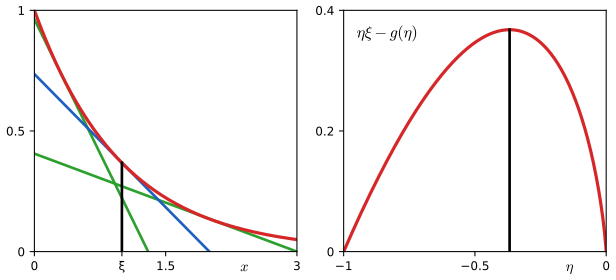
fig10_10. Download: PDF · SVG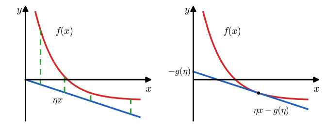
fig10_11. Download: PDF · SVGIf \(f\) is neither convex nor concave, look for an invertible transformation of the function or of its argument that makes it so, bound there, and transform back. The key example is the logistic sigmoid
\[ \sigma(x)=\frac1{1+e^{-x}}, \tag{10.134} \]which is neither: \(\sigma''\)
Result 10.21 (an exponential upper bound on the sigmoid) pp. 495–496 (10.135)–(10.137) Exercise 10.30
\(\ln\sigma(x)\) is concave, with conjugate (10.133) the binary entropy
\[ g(\eta)=\min_x\{\eta x-\ln\sigma(x)\}=-\eta\ln\eta-(1-\eta)\ln(1-\eta),\qquad0\lt\eta\lt1. \tag{10.135} \]Hence, for every \(\eta\in(0,1)\) and every \(x\),
\[ \ln\sigma(x)\le\eta x-g(\eta) \tag{10.136} \] \[ \sigma(x)\le\exp\big(\eta x-g(\eta)\big), \tag{10.137} \]with equality at \(x=\ln\{(1-\eta)/\eta\}\).
Proof
\(\frac{\d}{\d x}\ln\sigma(x)\)
(10.136) is (10.132) and (10.137) follows because \(\exp\) is increasing. Taylor route (Exercise 10.30): a concave function lies below its tangent, so \(\ln\sigma(x)\)
A lower bound of Gaussian form is more useful, because it combines with Gaussian priors. Following Jaakkola and Jordan (2000), transform both the function and its argument:
\[ \ln\sigma(x)=-\ln(1+e^{-x})=-\ln\big\{e^{-x/2}(e^{x/2}+e^{-x/2})\big\}=\frac x2-\ln\big(e^{x/2}+e^{-x/2}\big). \tag{10.138} \]Result 10.22 (the Jaakkola–Jordan bound) pp. 496–497 (10.139)–(10.144) Exercise 10.31
\(f(x)=-\ln(e^{x/2}+e^{-x/2})\) is concave in \(x\) but convex in \(x^2\). Its tangent in the variable \(x^2\) at \(x^2=\xi^2\) gives, for every \(\xi\) and every \(x\),
\[ \sigma(x)\ge\sigma(\xi)\exp\big\{(x-\xi)/2-\lambda(\xi)(x^2-\xi^2)\big\}, \tag{10.144} \] \[ \lambda(\xi)=\frac{1}{4\xi}\tanh\Big(\frac\xi2\Big)=\frac1{2\xi}\Big[\sigma(\xi)-\frac12\Big], \]with equality at \(x=\pm\xi\). The function \(\lambda\) is even and positive, \(\lambda(0)=\frac18\) (as a limit), it decreases strictly in \(|\xi|\), with \(\lambda'(\xi)\lt0\) for \(\xi\gt0\), and \(\lambda(\xi)\approx1/(4|\xi|)\) for large \(|\xi|\). The right side of (10.144) is the exponential of a quadratic in \(x\).
Proof
Concavity in \(x\). \(f(x)=-\ln(2\cosh\frac x2)\), \(f'(x)=-\frac12\tanh\frac x2\), \(f''(x)\)
Convexity in \(t=x^2\). \(f\) is even, so it is a function of \(t\ge0\): with \(u=\sqrt t\), \(f=-\ln(2\cosh\frac u2)\). By the chain rule (\(\d u/\d t=1/(2u)\)),
\[ \frac{\d f}{\d t}=-\frac{\tanh(u/2)}{4u},\qquad \frac{\d^2f}{\d t^2}=\frac{\tanh(u/2)-\frac u2\operatorname{sech}^2(u/2)}{8u^3}. \]Let \(h(v)\)
The tangent in \(t\). A convex function of \(t\) lies above its tangent at \(t_0=\xi^2\): \(f(x)\)
Back to the sigmoid. By (10.138) at \(x=\xi\), \(f(\xi)=\ln\sigma(\xi)-\xi/2\). So \(\ln\sigma(x)\)
Properties of \(\lambda\). \(\tanh(\xi/2)/\xi\) is even; \(\tanh(\xi/2)\approx\xi/2\) near 0 gives \(\lambda(0)=\frac18\); and \(\lambda'(\xi)\)
The book's conjugate-function route. With \(\eta\) the slope in \(x^2\), (10.129) reads
\[ g(\eta)=\max_{x^2}\big\{\eta x^2-f(\sqrt{x^2})\big\}, \tag{10.139} \]with stationarity condition
\[ 0=\eta-\frac{\d x}{\d x^2}\frac{\d}{\d x}f(x)=\eta+\frac1{4x}\tanh\Big(\frac x2\Big). \tag{10.140} \]Writing \(\xi\) for the contact point,
\[ \eta=-\frac1{4\xi}\tanh\Big(\frac\xi2\Big)=-\frac1{2\xi}\Big[\sigma(\xi)-\frac12\Big]=-\lambda(\xi), \tag{10.141} \] \[ g(\lambda(\xi))=-\lambda(\xi)\xi^2-f(\xi)=-\lambda(\xi)\xi^2+\ln\big(e^{\xi/2}+e^{-\xi/2}\big) \tag{10.142} \] \[ f(x)\ge-\lambda(\xi)x^2-g(\lambda(\xi))=-\lambda(\xi)x^2+\lambda(\xi)\xi^2-\ln\big(e^{\xi/2}+e^{-\xi/2}\big), \tag{10.143} \]which is the tangent inequality above.
Erratum. In the first printing (10.141) defines the variational parameter as \(\lambda\) (with sign conventions that clash with Jaakkola and Jordan), and (10.142)–(10.143) are correspondingly different. The corrected forms, used above, write \(\eta=-\lambda(\xi)\) and \(g(\lambda(\xi))\).
I checked (10.144) numerically on a fine grid of \(x\in[-30,30]\) for several \(\xi\): the gap \(\sigma(x)-\text{bound}\) is never negative and vanishes at \(\pm\xi\). The bound is only for two classes; for the softmax, Gibbs (1997) proposed a Gaussian-form construction that is conjectured, but not proved, to be a bound.
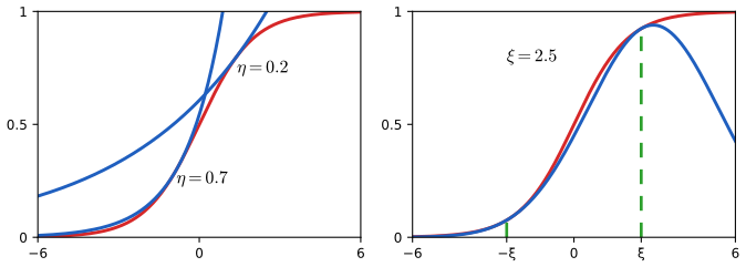
fig10_12. Download: PDF · SVGBounds inside integrals. The typical use is an integral such as
\[ I=\int\sigma(a)\,p(a)\,\d a \tag{10.145} \]with \(p(a)\) Gaussian (a predictive probability, say). Writing (10.144) as \(\sigma(a)\ge f(a,\xi)\), the integrand of
\[ I\ge\int f(a,\xi)\,p(a)\,\d a=F(\xi) \tag{10.146} \]is a product of two exponential-quadratic functions, so \(F\) is available in closed form, and we choose \(\xi^\star\) to maximise it. The bound is exact for one value of \(a\) only, so \(\xi^\star\) is a compromise weighted by \(p(a)\), and \(F(\xi^\star)\lt I\) in general.
Result 10.23 (the Gaussian integral of the bound)
For \(p(a)=\N(a\given\mu,s^2)\), put \(P=s^{-2}+2\lambda(\xi)\) and \(h=\mu/s^2+\frac12\). Then
\[ F(\xi)=\sigma(\xi)\exp\Big\{-\frac\xi2+\lambda(\xi)\xi^2\Big\}\big(1+2\lambda(\xi)s^2\big)^{-1/2}\exp\Big\{\frac{h^2}{2P}-\frac{\mu^2}{2s^2}\Big\}, \]and the stationary points of \(F\) are the solutions of \(\xi^2=P^{-1}+(h/P)^2\), the second moment of the normalised integrand \(f(a,\xi)p(a)\propto\N(a\given h/P,P^{-1})\). Iterating this equation increases \(F\) monotonically.
Proof
\(F(\xi)\)
For the maximiser, treat \(a\) as a latent variable and use the EM argument of Section 9.4: for \(\tilde q(a)\propto f(a,\xi^{\rm old})p(a)\), \(\ln F(\xi)\)
For example, with \(\mu=0.7\) and \(s^2=2.3\) I computed \(I=0.6210\) by quadrature, while the optimised bound is \(F(\xi^\star)=0.5974\) at \(\xi^\star=1.784\), found both by the fixed-point iteration and by direct maximisation. The bound is useful mostly inside larger computations, as in the next section.
10.6 Variational logistic regression
Return to Bayesian logistic regression (Section 4.5), where the Laplace approximation gave a Gaussian posterior. The variational treatment of Jaakkola and Jordan (2000) also gives a Gaussian, but it is fitted by maximising a rigorous lower bound on the evidence, with extra flexibility (one parameter per data point), and is more accurate than Laplace.
10.6.1 Variational posterior distribution
Take the Gaussian prior \(p(\mathbf{w})\)
and with \(a=\mathbf{w}^\T\bm\phi\) each likelihood term can be written as
\[ \begin{aligned}p(t\given\mathbf{w})&=\sigma(a)^t\{1-\sigma(a)\}^{1-t}=\Big(\frac1{1+e^{-a}}\Big)^t\Big(1-\frac1{1+e^{-a}}\Big)^{1-t}\\ &=e^{at}\frac{e^{-a}}{1+e^{-a}}=e^{at}\sigma(-a).\end{aligned} \tag{10.148} \](The third equality: \(1-\sigma(a)=e^{-a}/(1+e^{-a})\), so the product is \(e^{-a(1-t)}/(1+e^{-a})\)
Apply (10.149) with \(z=-a\) (and \((-a)^2=a^2\)):
\[ p(t\given\mathbf{w})=e^{at}\sigma(-a)\ge e^{at}\sigma(\xi)\exp\big\{-(a+\xi)/2-\lambda(\xi)(a^2-\xi^2)\big\}. \tag{10.151} \]The best \(\xi\) depends on \(a=\mathbf{w}^\T\bm\phi_n\), so each data point gets its own \(\xi_n\). Multiplying by the prior,
\[ p(\mathbf{t},\mathbf{w})=p(\mathbf{t}\given\mathbf{w})p(\mathbf{w})\ge h(\mathbf{w},\bm\xi)p(\mathbf{w}) \tag{10.152} \] \[ h(\mathbf{w},\bm\xi)=\prod_{n=1}^{N}\sigma(\xi_n)\exp\big\{\mathbf{w}^\T\bm\phi_nt_n-(\mathbf{w}^\T\bm\phi_n+\xi_n)/2-\lambda(\xi_n)([\mathbf{w}^\T\bm\phi_n]^2-\xi_n^2)\big\}. \tag{10.153} \]Normalising the left side of (10.152) would give the exact posterior, which is intractable; we normalise the right side instead. The resulting \(q(\mathbf{w})\) is a density, but no longer a bound. Taking logarithms (an increasing function preserves the inequality),
\[ \begin{aligned}\ln\{p(\mathbf{t}\given\mathbf{w})p(\mathbf{w})\}\ge\ln p(\mathbf{w})+\sum_{n=1}^{N}\big\{&\ln\sigma(\xi_n)+\mathbf{w}^\T\bm\phi_nt_n\\ &-(\mathbf{w}^\T\bm\phi_n+\xi_n)/2-\lambda(\xi_n)([\mathbf{w}^\T\bm\phi_n]^2-\xi_n^2)\big\},\end{aligned} \tag{10.154} \]and as a function of \(\mathbf{w}\) the right side is
\[ -\frac12(\mathbf{w}-\mathbf{m}_0)^\T\mathbf{S}_0^{-1}(\mathbf{w}-\mathbf{m}_0)+\sum_{n=1}^{N}\big\{\mathbf{w}^\T\bm\phi_n(t_n-1/2)-\lambda(\xi_n)\mathbf{w}^\T(\bm\phi_n\bm\phi_n^\T)\mathbf{w}\big\}+\const. \tag{10.155} \]Result 10.24 (the Gaussian variational posterior) p. 500, (10.156)–(10.158)
\[ q(\mathbf{w})=\N(\mathbf{w}\given\mathbf{m}_N,\mathbf{S}_N) \tag{10.156} \] \[ \mathbf{m}_N=\mathbf{S}_N\Big(\mathbf{S}_0^{-1}\mathbf{m}_0+\sum_{n=1}^{N}(t_n-1/2)\bm\phi_n\Big) \tag{10.157} \] \[ \mathbf{S}_N^{-1}=\mathbf{S}_0^{-1}+2\sum_{n=1}^{N}\lambda(\xi_n)\bm\phi_n\bm\phi_n^\T. \tag{10.158} \]Proof
Expand (10.155): the quadratic terms are \(-\frac12\mathbf{w}^\T\{\mathbf{S}_0^{-1}\)
Each data point acts as a Gaussian pseudo-observation of \(a_n=\mathbf{w}^\T\bm\phi_n\) with precision \(2\lambda(\xi_n)\) and pseudo-target \((t_n-\frac12)/(2\lambda(\xi_n))\). The Laplace approximation also adds a rank-one precision per point, \(\sigma_n(1-\sigma_n)\bm\phi_n\bm\phi_n^\T\) at the mode; here the curvature \(2\lambda(\xi_n)\) is chosen by optimising the evidence bound instead. Because the bound (10.154) is a sum of per-point terms, the posterior can also be updated one point at a time, \(\mathbf{S}_n^{-1}\)
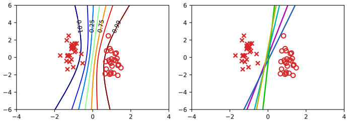
fig10_13. Download: PDF · SVG10.6.2 Optimising the variational parameters
The parameters \(\xi_n\) are chosen to maximise the bound on the log evidence obtained by substituting (10.152) into (10.147):
\[ \ln p(\mathbf{t})=\ln\int p(\mathbf{t}\given\mathbf{w})p(\mathbf{w})\,\d\mathbf{w}\ge\ln\int h(\mathbf{w},\bm\xi)p(\mathbf{w})\,\d\mathbf{w}=\LB(\bm\xi). \tag{10.159} \]As with the hyperparameters of linear regression (Section 3.5) there are two routes: treat \(\mathbf{w}\) as a latent variable and use EM, or do the Gaussian integral in closed form and maximise directly. They give the same fixed point.
EM. The E step computes \(q(\mathbf{w})\) of (10.156) at \(\bm\xi^{\rm old}\). The M step maximises the expected complete-data log likelihood
\[ Q(\bm\xi,\bm\xi^{\rm old})=\E\big[\ln\{h(\mathbf{w},\bm\xi)p(\mathbf{w})\}\big] \tag{10.160} \] \[ Q(\bm\xi,\bm\xi^{\rm old})=\sum_{n=1}^{N}\big\{\ln\sigma(\xi_n)-\xi_n/2-\lambda(\xi_n)(\bm\phi_n^\T\E[\mathbf{w}\mathbf{w}^\T]\bm\phi_n-\xi_n^2)\big\}+\const \tag{10.161} \](the expectation is under \(q(\mathbf{w})\) at \(\bm\xi^{\rm old}\); \(p(\mathbf{w})\) and the terms linear in \(\mathbf{w}\) do not involve \(\bm\xi\)). Setting \(\partial Q/\partial\xi_n=0\):
\[ 0=\lambda'(\xi_n)\big(\bm\phi_n^\T\E[\mathbf{w}\mathbf{w}^\T]\bm\phi_n-\xi_n^2\big) \tag{10.162} \] \[ (\xi_n^{\rm new})^2=\bm\phi_n^\T\E[\mathbf{w}\mathbf{w}^\T]\bm\phi_n=\bm\phi_n^\T\big(\mathbf{S}_N+\mathbf{m}_N\mathbf{m}_N^\T\big)\bm\phi_n. \tag{10.163} \]Erratum. The first printing writes \(\ln h(\mathbf{w},\bm\xi)p(\mathbf{w})\) in (10.160), without the braces.
Direct maximisation. The integral in (10.159) can be done in closed form:
\[ \begin{aligned}\LB(\bm\xi)&=\frac12\ln\frac{|\mathbf{S}_N|}{|\mathbf{S}_0|}+\frac12\mathbf{m}_N^\T\mathbf{S}_N^{-1}\mathbf{m}_N-\frac12\mathbf{m}_0^\T\mathbf{S}_0^{-1}\mathbf{m}_0\\ &\quad+\sum_{n=1}^{N}\Big\{\ln\sigma(\xi_n)-\frac12\xi_n+\lambda(\xi_n)\xi_n^2\Big\}.\end{aligned} \tag{10.164} \]Erratum. The first printing has several sign errors in (10.164); the form above is the corrected one.
Result 10.25 (the two routes agree) pp. 500–502 Exercises 10.33–10.35
(a) For each \(n\), \(Q\) is maximised over \(\xi_n\ge0\) exactly at (10.163), and the EM iteration never decreases \(\LB(\bm\xi)\). (b) \(\LB(\bm\xi)\) is given by (10.164), where \(\mathbf{m}_N,\mathbf{S}_N\) are (10.157)–(10.158) evaluated at \(\bm\xi\), and
\[ \frac{\partial\LB}{\partial\xi_n}=\lambda'(\xi_n)\Big\{\xi_n^2-\bm\phi_n^\T\big(\mathbf{S}_N+\mathbf{m}_N\mathbf{m}_N^\T\big)\bm\phi_n\Big\}, \]so the stationary points of \(\LB\) are exactly the fixed points of (10.163).
Filling the gap: "a few lines of algebra" for (10.162), and (10.164) pp. 501–502
Derivation
(10.161)–(10.163) (Exercise 10.33). In \(\ln h\), the \(n\)th term is \(\ln\sigma(\xi_n)+\mathbf{w}^\T\bm\phi_n(t_n-\frac12)\)
Since \(\lambda'(\xi)\lt0\) for \(\xi\gt0\) (Result 10.22), the derivative is positive for \(\xi_n^2\lt A_n\) and negative for \(\xi_n^2\gt A_n\): the unique maximiser on \(\xi_n\ge0\) is \(\xi_n=\sqrt{A_n}\), (10.163); \(\E[\mathbf{w}\mathbf{w}^\T]\)
(10.164) (Exercise 10.35). Write \(h(\mathbf{w},\bm\xi)p(\mathbf{w})\)
The Gaussian integral \(\int e^{-\frac12\mathbf{w}^\T\mathbf{A}\mathbf{w}+\mathbf{b}^\T\mathbf{w}}\d\mathbf{w}\)
The derivative (Exercise 10.34). Only \(\mathbf{S}_N\) depends on \(\bm\xi\) (\(\mathbf{b}\) does not), with \(\partial\mathbf{S}_N^{-1}/\partial\xi_n\)
and \(\frac{\d}{\d\xi}\{\ln\sigma(\xi)\)
Numerical checks. On a small two-dimensional problem, (10.164) agrees with direct numerical integration of \(h(\mathbf{w},\bm\xi)p(\mathbf{w})\) to eight digits, the EM iterates increase \(\LB\) monotonically to a value just below the exact \(\ln p(\mathbf{t})\), and the derivative formula agrees with finite differences.
Algorithm 10.5 (variational logistic regression)
- Initialise \(\xi_n\) (e.g. all equal to 1).
- E step. \(\mathbf{S}_N^{-1}\)
\({}=\mathbf{S}_0^{-1}\) \({}+2\sum_n\lambda(\xi_n)\bm\phi_n\bm\phi_n^\T\), \(\mathbf{m}_N\) \({}=\mathbf{S}_N(\mathbf{S}_0^{-1}\mathbf{m}_0+\sum_n(t_n-\frac12)\bm\phi_n)\). - M step. \(\xi_n\)
\({}=\big\{\bm\phi_n^\T(\mathbf{S}_N+\mathbf{m}_N\mathbf{m}_N^\T)\bm\phi_n\big\}^{1/2}\) for all \(n\). - Evaluate (10.164); repeat 2–4 until it stops increasing (typically a few iterations).
10.6.3 Inference of hyperparameters
Now let the prior precision be unknown, combining the global and local methods in one bound (as Bishop and Svensén 2003 did for hierarchical mixtures of experts):
\[ p(\mathbf{w}\given\alpha)=\N(\mathbf{w}\given\mathbf{0},\alpha^{-1}\mathbf{I}) \tag{10.165} \] \[ p(\alpha)=\Gam(\alpha\given a_0,b_0) \tag{10.166} \] \[ p(\mathbf{t})=\iint p(\mathbf{w},\alpha,\mathbf{t})\,\d\mathbf{w}\,\d\alpha \tag{10.167} \] \[ p(\mathbf{w},\alpha,\mathbf{t})=p(\mathbf{t}\given\mathbf{w})\,p(\mathbf{w}\given\alpha)\,p(\alpha). \tag{10.168} \]For any \(q(\mathbf{w},\alpha)\), Result 10.1 gives
\[ \ln p(\mathbf{t})=\LB(q)+\KL(q\|p) \tag{10.169} \] \[ \LB(q)=\iint q(\mathbf{w},\alpha)\ln\left\{\frac{p(\mathbf{w},\alpha,\mathbf{t})}{q(\mathbf{w},\alpha)}\right\}\d\mathbf{w}\,\d\alpha \tag{10.170} \] \[ \KL(q\|p)=-\iint q(\mathbf{w},\alpha)\ln\left\{\frac{p(\mathbf{w},\alpha\given\mathbf{t})}{q(\mathbf{w},\alpha)}\right\}\d\mathbf{w}\,\d\alpha. \tag{10.171} \]\(\LB(q)\) is still intractable because of \(p(\mathbf{t}\given\mathbf{w})\), so replace it by its lower bound \(h(\mathbf{w},\bm\xi)\) of (10.152)–(10.153); inside the logarithm this can only lower \(\LB\):
\[ \ln p(\mathbf{t})\ge\LB(q)\ge\tilde\LB(q,\bm\xi)=\iint q(\mathbf{w},\alpha)\ln\left\{\frac{h(\mathbf{w},\bm\xi)p(\mathbf{w}\given\alpha)p(\alpha)}{q(\mathbf{w},\alpha)}\right\}\d\mathbf{w}\,\d\alpha \tag{10.172} \]and assume \(q(\mathbf{w},\alpha)\)
Result 10.26 (the three updates) pp. 503–505, (10.174)–(10.183)
\[ q(\mathbf{w})=\N(\mathbf{w}\given\bm\mu_N,\bm\Sigma_N) \tag{10.174} \] \[ \bm\Sigma_N^{-1}\bm\mu_N=\sum_{n=1}^{N}(t_n-1/2)\bm\phi_n \tag{10.175} \] \[ \bm\Sigma_N^{-1}=\E[\alpha]\mathbf{I}+2\sum_{n=1}^{N}\lambda(\xi_n)\bm\phi_n\bm\phi_n^\T \tag{10.176} \] \[ q(\alpha)=\Gam(\alpha\given a_N,b_N)=\frac1{\Gamma(a_N)}b_N^{a_N}\alpha^{a_N-1}e^{-b_N\alpha} \tag{10.177} \] \[ a_N=a_0+\frac M2 \tag{10.178} \] \[ b_N=b_0+\frac12\E_{\mathbf{w}}[\mathbf{w}^\T\mathbf{w}] \tag{10.179} \] \[ (\xi_n^{\rm new})^2=\bm\phi_n^\T\big(\bm\Sigma_N+\bm\mu_N\bm\mu_N^\T\big)\bm\phi_n \tag{10.181} \]with the moments
\[ \E[\alpha]=\frac{a_N}{b_N} \tag{10.182} \] \[ \E[\mathbf{w}\mathbf{w}^\T]=\bm\Sigma_N+\bm\mu_N\bm\mu_N^\T. \tag{10.183} \]Each update maximises \(\tilde\LB\) over its own argument, so cycling through them never decreases \(\tilde\LB\).
Erratum. The first printing has \(a_0,b_0\) instead of \(a_N,b_N\) on the right of (10.177), the transposes misplaced in (10.183), and refers to (10.159) instead of (10.160) when introducing (10.181).
Filling the gap: the updates, and a bound to monitor pp. 504–505
Derivation
\(q(\mathbf{w})\). By (10.9) applied to the integrand of (10.172), \(\ln q(\mathbf{w})\)
which is (10.155) with \(\mathbf{m}_0=\mathbf{0}\) and \(\mathbf{S}_0^{-1}\) replaced by \(\E[\alpha]\mathbf{I}\); completing the square gives (10.174)–(10.176).
\(q(\alpha)\). \(\ln q(\alpha)\)
\(\bm\xi\). Dropping the terms of \(\tilde\LB\) that do not involve \(\bm\xi\) and integrating over \(\alpha\),
\[ \tilde\LB(q,\bm\xi)=\int q(\mathbf{w})\ln h(\mathbf{w},\bm\xi)\,\d\mathbf{w}+\const, \tag{10.180} \]which has the same \(\bm\xi\)-dependence as \(Q\) in (10.160)–(10.161). The maximiser is (10.163) with the current \(q(\mathbf{w})\), i.e. (10.181).
The bound, for monitoring. All five pieces are explicit:
\[ \begin{aligned}\tilde\LB&=\sum_n\Big\{\ln\sigma(\xi_n)+(t_n-\tfrac12)\bm\mu_N^\T\bm\phi_n-\tfrac{\xi_n}2-\lambda(\xi_n)\big(\bm\phi_n^\T\E[\mathbf{w}\mathbf{w}^\T]\bm\phi_n-\xi_n^2\big)\Big\}\\ &\quad+\E[\ln p(\mathbf{w}\given\alpha)]+\E[\ln p(\alpha)]+\mathrm{H}[q(\mathbf{w})]+\mathrm{H}[q(\alpha)],\end{aligned} \]where the last four terms are (10.109)–(10.112) with \(\mathbf{m}_N,\mathbf{S}_N\) replaced by \(\bm\mu_N,\bm\Sigma_N\). In a numerical check this quantity increased at each of the three updates. ∎
10.7 Expectation propagation
Expectation propagation (EP; Minka 2001a, 2001b) is also based on a KL divergence, but the reverse one, \(\KL(p\|q)\), and only locally. Its basic step is the following fact about exponential families. Let
\[ q(\mathbf{z})=h(\mathbf{z})\,g(\bm\eta)\exp\big\{\bm\eta^\T\mathbf{u}(\mathbf{z})\big\} \tag{10.184} \](the form (2.194)). As a function of \(\bm\eta\), for a fixed \(p\),
\[ \KL(p\|q)=-\ln g(\bm\eta)-\bm\eta^\T\E_{p(\mathbf{z})}[\mathbf{u}(\mathbf{z})]+\const. \tag{10.185} \]Result 10.27 (moment matching) pp. 505–506 (10.186)–(10.187) Exercise 10.4
\(\KL(p\|q_{\bm\eta})\) is a convex function of \(\bm\eta\), and \(\bm\eta\) minimises it if and only if
\[ -\nabla\ln g(\bm\eta)=\E_{p(\mathbf{z})}[\mathbf{u}(\mathbf{z})] \tag{10.186} \] \[ \text{equivalently}\qquad \E_{q(\mathbf{z})}[\mathbf{u}(\mathbf{z})]=\E_{p(\mathbf{z})}[\mathbf{u}(\mathbf{z})]: \tag{10.187} \]the best member of the family matches the expected sufficient statistics of \(p\). For a Gaussian \(q\) (\(\mathbf{u}\)
Proof
\(\KL(p\|q)\)
This is the "moment matching" seen in Figure 10.3(a) and in the first row of the table after Result 10.2.
The EP approximation. Many joint densities are products of factors,
\[ p(\mathcal{D},\bm\theta)=\prod_if_i(\bm\theta), \tag{10.188} \]for example \(f_0(\bm\theta)=p(\bm\theta)\) and \(f_n(\bm\theta)\)
EP approximates the posterior by a product of the same shape, with each factor replaced by a member of an exponential family (so that \(q\) itself is in that family, e.g. Gaussian):
\[ q(\bm\theta)=\frac1Z\prod_i\tilde f_i(\bm\theta). \tag{10.191} \]Ideally we would minimise
\[ \KL(p\|q)=\KL\Big(\frac1{p(\mathcal{D})}\prod_if_i(\bm\theta)\,\Big\|\,\frac1Z\prod_i\tilde f_i(\bm\theta)\Big), \tag{10.192} \]but that needs expectations under the true posterior. Fitting each \(\tilde f_i\) to \(f_i\) in isolation is easy and non-iterative but can be poor, because a factor need only be accurate where the posterior has mass. EP fits each factor in the context of the others: to refine \(\tilde f_j\), make
\[ q^{\rm new}(\bm\theta)\propto\tilde f_j(\bm\theta)\prod_{i\ne j}\tilde f_i(\bm\theta) \tag{10.193} \]as close as possible to
\[ f_j(\bm\theta)\prod_{i\ne j}\tilde f_i(\bm\theta) \tag{10.194} \]with the other factors fixed. Concretely, remove \(\tilde f_j\) to get the cavity distribution
\[ q^{\setminus j}(\bm\theta)=\frac{q(\bm\theta)}{\tilde f_j(\bm\theta)}, \tag{10.195} \]multiply by the true factor to get the tilted distribution
\[ \frac1{Z_j}f_j(\bm\theta)\,q^{\setminus j}(\bm\theta) \tag{10.196} \] \[ Z_j=\int f_j(\bm\theta)\,q^{\setminus j}(\bm\theta)\,\d\bm\theta, \tag{10.197} \]and choose \(q^{\rm new}\) in the family to minimise
\[ \KL\Big(\frac{f_j(\bm\theta)q^{\setminus j}(\bm\theta)}{Z_j}\,\Big\|\,q^{\rm new}(\bm\theta)\Big), \tag{10.198} \]which by Result 10.27 means matching the moments of the tilted distribution (for any exponential family whose moments can be related to the derivatives of its normaliser, (2.226)). The new factor is then obtained by division,
\[ \tilde f_j(\bm\theta)=K\frac{q^{\rm new}(\bm\theta)}{q^{\setminus j}(\bm\theta)}. \tag{10.199} \]Filling the gap: why \(K=Z_j\) pp. 508–509, (10.199)–(10.201)
Derivation
Multiply (10.199) by \(q^{\setminus j}\) and integrate; since \(q^{\rm new}\) is normalised,
\[ K=\int\tilde f_j(\bm\theta)\,q^{\setminus j}(\bm\theta)\,\d\bm\theta. \tag{10.200} \]The moment matching fixes the normalised shape of \(\tilde f_jq^{\setminus j}\)
gives \(K=Z_j\) by (10.197). The constant has no effect on \(q\), which is normalised anyway; it matters only for the evidence approximation (10.208). ∎
Erratum. On p. 509, line 1, \(q^{\setminus i}(\bm\theta)\) should be \(q^{\setminus j}(\bm\theta)\).
Algorithm 10.6 (expectation propagation) pp. 509–510, (10.202)–(10.208)
Given \(p(\mathcal{D},\bm\theta)\)
- Initialise the factors \(\tilde f_i(\bm\theta)\).
- Set \(q(\bm\theta)\propto\prod_i\tilde f_i(\bm\theta)\) (10.204).
- Until convergence: (a) choose a factor \(\tilde f_j\); (b) form the cavity \(q^{\setminus j}(\bm\theta)\)
\({}=q(\bm\theta)/\tilde f_j(\bm\theta)\) (10.205); (c) set the sufficient statistics (moments) of \(q^{\rm new}\) equal to those of \(q^{\setminus j}(\bm\theta)f_j(\bm\theta)\), and compute \(Z_j\) \({}=\int q^{\setminus j}(\bm\theta)f_j(\bm\theta)\d\bm\theta\) (10.206); (d) store \(\tilde f_j(\bm\theta)\) \({}=Z_jq^{\rm new}(\bm\theta)/q^{\setminus j}(\bm\theta)\) (10.207) and set \(q=q^{\rm new}\). - Approximate the evidence by
In an exponential family, the divisions (10.205) and (10.207) are subtractions of natural parameters (for Gaussians, of precisions and precision-times-means; toolkit: Gaussian facts). A factor \(\tilde f_j\) need not be a normalisable density, but the cavity must be for step (c); if it is not, skip that update.
At a fixed point, \(q\) has exactly the moments of every tilted distribution \(q^{\setminus j}f_j\): this "moment consistency" is what EP achieves instead of the intractable global minimisation of (10.192).
Assumed density filtering (ADF, also called moment matching; see the references on p. 510 of the book) is the special case in which all factors except the first are initialised to 1 and each is updated once, in a single pass: suitable for on-line learning, but in batch use its answer depends on the arbitrary order of the data. Its evidence estimate is \(\prod_jZ_j\) (Exercise 10.36). EP revisits the factors until they agree, which removes the order dependence and improves accuracy.
Properties. EP is not guaranteed to converge. When \(q\) is in an exponential family and it does converge, the fixed point is a stationary point of a certain energy function (Minka 2001a), though the iterations need not decrease it; algorithms that minimise that energy directly converge, but are slower and more complex. Variational Bayes, by contrast, increases its bound at every step. Because EP minimises \(\KL(p\|q)\) locally, it averages over modes, which makes it a poor choice for mixture posteriors; for logistic-type models it is often more accurate than both local variational bounds and Laplace (Kuss and Rasmussen 2005).
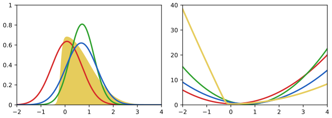
fig10_14. Download: PDF · SVGErratum. In the caption of Figure 10.14, "obtained by" should be inserted between "that" and "variational".
10.7.1 Example: the clutter problem
Following Minka (2001b): infer the mean \(\bm\theta\) of a \(D\)-dimensional Gaussian from observations embedded in background clutter,
\[ p(\mathbf{x}\given\bm\theta)=(1-w)\N(\mathbf{x}\given\bm\theta,\mathbf{I})+w\N(\mathbf{x}\given\mathbf{0},a\mathbf{I}) \tag{10.209} \] \[ p(\bm\theta)=\N(\bm\theta\given\mathbf{0},b\mathbf{I}) \tag{10.210} \] \[ p(\mathcal{D},\bm\theta)=p(\bm\theta)\prod_{n=1}^{N}p(\mathbf{x}_n\given\bm\theta) \tag{10.211} \]with the clutter fraction \(w\) known; Minka uses \(a=10\), \(b=100\), \(w=0.5\). Expanding the product, the posterior is a mixture of \(2^N\) Gaussians (each data point is either signal or clutter), so exact inference costs \(O(2^N)\). For EP take \(f_0=p(\bm\theta)\), \(f_n=p(\mathbf{x}_n\given\bm\theta)\), and a spherical Gaussian
\[ q(\bm\theta)=\N(\bm\theta\given\mathbf{m},v\mathbf{I}), \tag{10.212} \]so the factor approximations are exponential-quadratic,
\[ \tilde f_n(\bm\theta)=s_n\N(\bm\theta\given\mathbf{m}_n,v_n\mathbf{I}), \tag{10.213} \]for \(n=1,\dots,N\), with \(\tilde f_0=p(\bm\theta)\). Here \(\N\) is only notation: \(v_n\) may be negative or infinite. Initialising \(\tilde f_n=1\) (\(s_n=(2\pi v_n)^{D/2}\), \(v_n\to\infty\), \(\mathbf{m}_n=\mathbf{0}\)) makes the initial \(q\) equal to the prior; the prior factor is already in the family and is never changed by an EP update (Exercise 10.37).
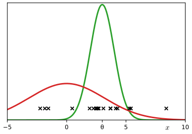
fig10_15. Download: PDF · SVGResult 10.28 (EP updates for the clutter problem) pp. 512–513 (10.214)–(10.224) Exercises 10.38 10.39
To refine \(\tilde f_n\): the cavity has mean and inverse variance
\[ \mathbf{m}^{\setminus n}=\mathbf{m}+v^{\setminus n}v_n^{-1}(\mathbf{m}-\mathbf{m}_n) \tag{10.214} \] \[ (v^{\setminus n})^{-1}=v^{-1}-v_n^{-1}; \tag{10.215} \]the normaliser of the tilted distribution is
\[ Z_n=(1-w)\N\big(\mathbf{x}_n\given\mathbf{m}^{\setminus n},(v^{\setminus n}+1)\mathbf{I}\big)+w\N(\mathbf{x}_n\given\mathbf{0},a\mathbf{I}); \tag{10.216} \]the matched moments are
\[ \mathbf{m}^{\rm new}=\mathbf{m}^{\setminus n}+\rho_n\frac{v^{\setminus n}}{v^{\setminus n}+1}(\mathbf{x}_n-\mathbf{m}^{\setminus n}) \tag{10.217} \] \[ v^{\rm new}=v^{\setminus n}-\rho_n\frac{(v^{\setminus n})^2}{v^{\setminus n}+1}+\rho_n(1-\rho_n)\frac{(v^{\setminus n})^2\|\mathbf{x}_n-\mathbf{m}^{\setminus n}\|^2}{D(v^{\setminus n}+1)^2} \tag{10.218} \] \[ \rho_n=1-\frac{w}{Z_n}\N(\mathbf{x}_n\given\mathbf{0},a\mathbf{I}), \tag{10.219} \]where \(\rho_n\) is the probability, under the cavity, that \(\mathbf{x}_n\) is not clutter; and the refined factor has
\[ v_n^{-1}=(v^{\rm new})^{-1}-(v^{\setminus n})^{-1} \tag{10.220} \] \[ \mathbf{m}_n=\mathbf{m}^{\setminus n}+(v_n+v^{\setminus n})(v^{\setminus n})^{-1}(\mathbf{m}^{\rm new}-\mathbf{m}^{\setminus n}) \tag{10.221} \] \[ s_n=\frac{Z_n}{(2\pi v_n)^{D/2}\N\big(\mathbf{m}_n\given\mathbf{m}^{\setminus n},(v_n+v^{\setminus n})\mathbf{I}\big)}. \tag{10.222} \]After convergence (\(\mathbf{m}=\mathbf{m}^{\rm new}\), \(v=v^{\rm new}\)) the evidence (10.208) is evaluated with
\[ p(\mathcal{D})\simeq(2\pi v^{\rm new})^{D/2}\exp(B/2)\prod_{n=1}^{N}\big\{s_n(2\pi v_n)^{-D/2}\big\} \tag{10.223} \] \[ B=\frac{(\mathbf{m}^{\rm new})^\T\mathbf{m}^{\rm new}}{v^{\rm new}}-\sum_{n=1}^{N}\frac{\mathbf{m}_n^\T\mathbf{m}_n}{v_n}, \tag{10.224} \]subject to the correction in the note below.
Erratum. In (10.217) and (10.218) the left sides read \(\mathbf{m}\) and \(v\) in the book (also in the printing used here); they are \(\mathbf{m}^{\rm new}\) and \(v^{\rm new}\). In (10.245) of Exercise 10.39 the term \(v^{\setminus n}D\) is missing in early printings.
Note on (10.222) and (10.223)
The two formulas use different conventions for \(s_n\). The factor (10.222) is the right normaliser if the site is written \(\tilde f_n\)
with \(B\) as in (10.224); equivalently, (10.223) is correct in the convention of (10.213) if its product starts at \(n=0\), with the prior written as a site (\(s_0=1\), \(\mathbf{m}_0=\mathbf{0}\), \(v_0=b\)). I checked this on a one-dimensional clutter data set with \(N=20\): the formula above agrees with direct numerical integration of \(\prod_i\tilde f_i\) to \(10^{-6}\) (and is within 0.005 of the exact \(\ln p(\mathcal{D})\)), whereas combining (10.222) and (10.223) literally is off by about 31 in \(\ln p(\mathcal{D})\). The updates (10.214)–(10.221), and hence \(q\), are unaffected. As a sanity check, with \(w=0\) every factor is Gaussian, EP is exact, and this formula returns the exact evidence.
Filling the gap: the cavity (10.214)–(10.215) and \(Z_n\) (10.216) p. 512, Exercise 10.38
Derivation
Cavity. Up to constants, \(\ln q^{\setminus n}\)
Normaliser. With the normalised cavity \(\N(\bm\theta\given\mathbf{m}^{\setminus n},v^{\setminus n}\mathbf{I})\),
\[ Z_n=(1-w)\int\N(\mathbf{x}_n\given\bm\theta,\mathbf{I})\N(\bm\theta\given\mathbf{m}^{\setminus n},v^{\setminus n}\mathbf{I})\,\d\bm\theta+w\N(\mathbf{x}_n\given\mathbf{0},a\mathbf{I})\int\N(\bm\theta\given\mathbf{m}^{\setminus n},v^{\setminus n}\mathbf{I})\,\d\bm\theta. \]The second integral is 1. The first is the marginal of \(\mathbf{x}_n=\bm\theta+\bm\epsilon\) in a linear-Gaussian model (2.115) (toolkit): \(\N(\mathbf{x}_n\given\mathbf{m}^{\setminus n},(v^{\setminus n}+1)\mathbf{I})\). This is (10.216). ∎
Filling the gap: the moments (10.217)–(10.219) via (10.244)–(10.245) p. 512, Exercise 10.39
The book says "we compute the mean and variance of \(q^{\rm new}\) by finding the mean and variance of \(q^{\setminus n}f_n\)" and leaves the details to the reader. The neat way is to differentiate \(\ln Z_n\) with respect to the cavity parameters.
Derivation
Two general identities. Let \(Z(\mathbf{m},v)\)
the second because \(\E\|\bm\theta-\mathbf{m}\|^2\)
Apply to \(Z_n\). Only the first term of (10.216) depends on \((\mathbf{m},v)\). Write \(\N_1\)
(10.244) now gives (10.217). For the variance, \(q^{\rm new}\) is spherical, so \(v^{\rm new}\)
and dividing by \(D\) gives (10.218). ∎
Reading the formulas. If \(\rho_n=1\) (certainly signal) they reduce to the conjugate Gaussian update, \(\mathbf{m}^{\rm new}\)
Filling the gap: the refined factor (10.220)–(10.222) and the evidence (10.223)–(10.224) pp. 512–513, Exercise 10.39
Derivation
Shape. By (10.207), \(\tilde f_n\)
Scale. Write the factor as \(\tilde f_n\)
(toolkit; when \(v_n\lt0\), read the constant \((2\pi v_n)^{D/2}\N(\mathbf{m}_n\given\cdots)\) as the single real number \(\big(\frac{v_n}{v_n+v^{\setminus n}}\big)^{D/2}\exp\{-\frac{\|\mathbf{m}_n-\mathbf{m}^{\setminus n}\|^2}{2(v_n+v^{\setminus n})}\}\), positive because \(\frac{v_n}{v_n+v^{\setminus n}}\)
Evidence. By (10.208), \(p(\mathcal{D})\simeq\int\tilde f_0\prod_n\tilde f_n\,\d\bm\theta\) with \(\tilde f_0\)
where \(1/v=\sum_{n=0}^N1/v_n\) and \(\mathbf{m}/v\)
Algorithm 10.7 (EP for the clutter problem)
- Set all sites to 1 (\(v_n^{-1}=0\), \(\mathbf{m}_n/v_n=\mathbf{0}\)), so \(q=p(\bm\theta)\): \(\mathbf{m}=\mathbf{0}\), \(v=b\).
- For \(n=1,\dots,N\) in turn: compute the cavity (10.214)–(10.215) (skip \(n\) if \(v^{\setminus n}\le0\)); \(Z_n\) and \(\rho_n\) (10.216), (10.219); \(\mathbf{m}^{\rm new},v^{\rm new}\) (10.217)–(10.218); the site (10.220)–(10.222); set \(\mathbf{m}=\mathbf{m}^{\rm new}\), \(v=v^{\rm new}\).
- Repeat step 2 until the largest change in the site parameters over a sweep is below a tolerance.
- Evaluate the evidence with the corrected (10.223) of the note above.
EP has no guarantee of reaching a good fixed point: in a single sweep from the prior, two outlying clutter points processed first can pull the cavity towards themselves and steer the iteration to a poor solution, so it is worth comparing runs with different orders (or damping the updates).
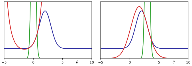
fig10_16. Download: PDF · SVGErratum. On p. 513, the first line after (10.224) should read "Examples of factor approximations".
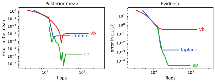
fig10_17. Download: PDF · SVG10.7.2 Expectation propagation on graphs
Now let each factor depend on a subset of the variables, as in a factor graph (Section 8.4.3). We show that EP with a fully factorised \(q\) is loopy belief propagation (Minka 2001a). Start with the factor graph of Figure 8.51,
\[ p(\mathbf{x})=f_a(x_1,x_2)\,f_b(x_2,x_3)\,f_c(x_2,x_4). \tag{10.225} \]Seek \(q\) with the same factorisation,
\[ q(\mathbf{x})\propto\tilde f_a(x_1,x_2)\,\tilde f_b(x_2,x_3)\,\tilde f_c(x_2,x_4), \tag{10.226} \]with normalisation restored locally at the end, and restrict each approximate factor to factorise over its variables (Figure 10.18, right):
\[ q(\mathbf{x})\propto\tilde f_{a1}(x_1)\tilde f_{a2}(x_2)\tilde f_{b2}(x_2)\tilde f_{b3}(x_3)\tilde f_{c2}(x_2)\tilde f_{c4}(x_4). \tag{10.227} \]Then \(q\) is fully factorised. To refine \(\tilde f_b(x_2,x_3)\)
Erratum. The first printing has "=" instead of "\(\propto\)" in (10.228), and \(\tilde f\) is mistyped in the labels of Figure 10.18 (right).
By Result 10.6, minimising \(\KL(\hat p\|q^{\rm new})\) over fully factorised \(q^{\rm new}\) gives the product of the marginals of \(\hat p\):
\[ \hat p(x_1)\propto\tilde f_{a1}(x_1) \tag{10.230} \] \[ \hat p(x_2)\propto\tilde f_{a2}(x_2)\tilde f_{c2}(x_2)\sum_{x_3}f_b(x_2,x_3) \tag{10.231} \] \[ \hat p(x_3)\propto\sum_{x_2}\big\{f_b(x_2,x_3)\tilde f_{a2}(x_2)\tilde f_{c2}(x_2)\big\} \tag{10.232} \] \[ \hat p(x_4)\propto\tilde f_{c4}(x_4). \tag{10.233} \]Dividing \(q^{\rm new}\) by \(q^{\setminus b}\) gives the refined factor:
\[ \tilde f_{b2}(x_2)\propto\sum_{x_3}f_b(x_2,x_3) \tag{10.234} \] \[ \tilde f_{b3}(x_3)\propto\sum_{x_2}\big\{f_b(x_2,x_3)\tilde f_{a2}(x_2)\tilde f_{c2}(x_2)\big\}. \tag{10.235} \]Filling the gap: the marginals (10.230)–(10.235) p. 515
Derivation
Marginalise (10.229) one variable at a time (sums for discrete variables, integrals otherwise). For \(x_1\): \(\hat p(x_1)\propto\tilde f_{a1}(x_1)\)
These are exactly the belief-propagation messages with the variable-to-factor messages folded into the factor-to-variable messages (Section 8.4.4): \(\tilde f_{b2}(x_2)\) is \(\mu_{f_b\to x_2}(x_2)\) of (8.81), and substituting (8.78) into (8.79) gives (10.235), with \(\tilde f_{a2}=\mu_{f_a\to x_2}\) and \(\tilde f_{c2}=\mu_{f_c\to x_2}\), so that \(\tilde f_{b3}=\mu_{f_b\to x_3}\). EP sends the messages in both directions at once; refining one sub-factor at a time (for example only \(\tilde f_{b3}\)) gives the usual sum-product schedule, and on a tree the two-pass schedule gives exact marginals whatever the initialisation.
General factor graphs. For
\[ p(\bm\theta)=\prod_if_i(\bm\theta_i), \tag{10.236} \]with \(\bm\theta_i\) the variables of factor \(i\), use the fully factorised approximation
\[ q(\bm\theta)\propto\prod_i\prod_k\tilde f_{ik}(\theta_k), \tag{10.237} \]where \(\theta_k\) runs over the variable nodes (with \(\tilde f_{ik}\equiv1\) if \(\theta_k\notin\bm\theta_i\)). To refine \(\tilde f_{jl}(\theta_l)\), remove \(\tilde f_j(\bm\theta_j)\),
\[ q^{\setminus j}(\bm\theta)\propto\prod_{i\ne j}\prod_k\tilde f_{ik}(\theta_k), \tag{10.238} \]and take the marginal on \(\theta_l\) of
\[ q^{\setminus j}(\bm\theta)f_j(\bm\theta_j). \tag{10.239} \]Result 10.29 (fully factorised EP is belief propagation) pp. 516–517, (10.240)
\[ \tilde f_{jl}(\theta_l)\propto\sum_{\theta_{m\ne l}\in\bm\theta_j}f_j(\bm\theta_j)\prod_{k}\prod_{m\ne l}\tilde f_{km}(\theta_m), \tag{10.240} \]where the product runs over the factors \(k\ne j\) and over the variables \(m\ne l\) of \(f_j\). With \(\tilde f_{km}(\theta_m)\)
Proof
Marginalise (10.239) onto \(\theta_l\). Split the factors \(\tilde f_{ik}(\theta_k)\), \(i\ne j\), of \(q^{\setminus j}\) into three groups: those with \(k=l\), which are functions of \(\theta_l\) and come out of the sum as \(\prod_{i\ne j}\tilde f_{il}(\theta_l)\); those with \(\theta_k\in\bm\theta_j\), \(k\ne l\), which stay inside the sum over \(\bm\theta_j\setminus\theta_l\) together with \(f_j\); and those with \(\theta_k\notin\bm\theta_j\), which sum to constants. Moment matching for a fully factorised \(q\) sets the new \(\theta_l\)-factor of \(q\) to this marginal (Result 10.6). Dividing by the \(\theta_l\)-factor of \(q^{\setminus j}\), which is \(\prod_{i\ne j}\tilde f_{il}(\theta_l)\), leaves (10.240): the terms of the other factors cancel between numerator and denominator. ∎
So the sum-product algorithm is the special case of EP with the most factorised \(q\). Less factorised approximations (partially disconnected graphs) and refining groups of factors together can both be more accurate (Minka 2001b); choosing them well is an open problem. More generally, Minka (2005) shows that variational message passing, loopy belief propagation and EP, as well as tree-reweighted message passing (Wainwright et al. 2005), fractional belief propagation (Wiegerinck and Heskes 2003) and power EP (Minka 2004), all minimise local alpha-divergences (10.19) for different \(\alpha\) (Result 10.7).
Exercises
All 39 exercises of Chapter 10 (pp. 517–522), restated briefly, with full solutions (hidden). The www exercises are those with official solutions (Svensén and Bishop 2009); the others are solved here independently. Where the main text already contains the complete derivation, the solution gives the argument in short form and links to it.
Exercise 10.1 (www). Show that \(\ln p(\mathbf{X})=\LB(q)+\KL(q\|p)\) with \(\LB\) and \(\KL\) as in (10.3) and (10.4).
Solution
By the product rule, \(\ln\{p(\mathbf{X},\mathbf{Z})/q(\mathbf{Z})\}\)
\({}=\ln\{p(\mathbf{Z}\given\mathbf{X})/q(\mathbf{Z})\}+\ln p(\mathbf{X})\). Multiply by \(q(\mathbf{Z})\) and integrate; since \(\int q=1\), \(\LB(q)\) \({}=-\KL(q\|p)+\ln p(\mathbf{X})\). Details and consequences: Result 10.1. Exercise 10.2. Using \(\E[z_1]=m_1\), \(\E[z_2]=m_2\), solve (10.13) and (10.15) and show that for non-singular \(p\) the unique solution is \(\E[z_i]=\mu_i\).
Solution
With \(e_i=m_i-\mu_i\) the equations are \(e_1\)
\({}=-(\Lambda_{12}/\Lambda_{11})e_2\) and \(e_2\) \({}=-(\Lambda_{21}/\Lambda_{22})e_1\), so \(e_1(1-\rho^2)=0\) with \(\rho^2\) \({}=\Lambda_{12}^2/(\Lambda_{11}\Lambda_{22})\). Non-singularity of the positive definite \(\bm\Lambda\) means \(\Lambda_{11}\Lambda_{22}-\Lambda_{12}^2\) \({}\gt0\), i.e. \(\rho^2\lt1\); hence \(e_1=0\) and then \(e_2=0\). If \(\bm\Lambda\) were singular (\(\rho^2=1\)), every point of the line \(e_1\) \({}=-(\Lambda_{12}/\Lambda_{11})e_2\) would solve both equations, so uniqueness fails. See Result 10.5. Exercise 10.3 (www). For factorised \(q\), use a Lagrange multiplier to show that minimising \(\KL(p\|q)\) over one factor \(q_j\) gives (10.17).
Solution
By (10.16), the terms of \(\KL(p\|q)\) that involve \(q_j\) are \(-\int p(\mathbf{Z})\ln q_j(\mathbf{Z}_j)\,\d\mathbf{Z}\)
\({}=-\int F_j(\mathbf{Z}_j)\ln q_j(\mathbf{Z}_j)\,\d\mathbf{Z}_j\) with \(F_j(\mathbf{Z}_j)\) \({}=\int p(\mathbf{Z})\prod_{i\ne j}\d\mathbf{Z}_i\). Minimise \(-\int F_j\ln q_j+\lambda(\int q_j-1)\). The functional derivative is \(-F_j/q_j+\lambda=0\), so \(q_j=F_j/\lambda\), and integrating, \(\lambda=\int F_j\,\d\mathbf{Z}_j=1\). Hence \(q_j^\star=F_j=p_j\), the marginal. The second variation \(\int F_j(\delta q_j)^2/q_j^2\gt0\) shows it is a minimum. (A shorter route is the decomposition in Result 10.6.) Exercise 10.4. For fixed \(p(\mathbf{x})\) and Gaussian \(q(\mathbf{x})\)
\({}=\N(\mathbf{x}\given\bm\mu,\bm\Sigma)\), show by differentiation that \(\KL(p\|q)\) is minimised when \(\bm\mu\) and \(\bm\Sigma\) are the mean and covariance of \(p\). Solution
Let \(\mathbf{m}=\E_p[\mathbf{x}]\), \(\mathbf{C}=\cov_p[\mathbf{x}]\) and \(\bm\Lambda=\bm\Sigma^{-1}\). Up to terms not involving \(q\),
\[ \begin{aligned}\KL(p\|q)&=-\E_p[\ln\N(\mathbf{x}\given\bm\mu,\bm\Sigma)]=-\tfrac12\ln|\bm\Lambda|+\tfrac12\E_p[(\mathbf{x}-\bm\mu)^\T\bm\Lambda(\mathbf{x}-\bm\mu)]\\ &=-\tfrac12\ln|\bm\Lambda|+\tfrac12\Tr\big(\bm\Lambda\{\mathbf{C}+(\mathbf{m}-\bm\mu)(\mathbf{m}-\bm\mu)^\T\}\big).\end{aligned} \]The gradient in \(\bm\mu\) is \(-\bm\Lambda(\mathbf{m}-\bm\mu)\), zero iff \(\bm\mu=\mathbf{m}\). Then the gradient in \(\bm\Lambda\) is \(-\frac12\bm\Lambda^{-1}\)
\({}+\frac12\mathbf{C}\) (toolkit: matrix calculus), zero iff \(\bm\Sigma=\mathbf{C}\). The function is convex in \((\bm\mu,\bm\Lambda)\) separately (a positive definite quadratic in \(\bm\mu\); \(-\ln|\bm\Lambda|\) is convex and the trace is linear), so this stationary point is the minimum. This is the Gaussian case of Result 10.27. Exercise 10.5 (www). With \(q(\mathbf{z},\bm\theta)\)
\({}=q_{\mathbf{z}}(\mathbf{z})q_{\bm\theta}(\bm\theta)\) and \(q_{\bm\theta}\) \({}=\delta(\bm\theta-\bm\theta_0)\), show that variational optimisation is EM: the E step optimises \(q_{\mathbf{z}}\), the M step maximises the expected complete-data log posterior over \(\bm\theta_0\). Solution
E step. By (10.9), \(\ln q_{\mathbf{z}}(\mathbf{z})\)
\({}=\E_{\bm\theta}[\ln p(\mathbf{X},\mathbf{z},\bm\theta)]+\const\) \({}=\ln p(\mathbf{X},\mathbf{z},\bm\theta_0)+\const\), so \(q_{\mathbf{z}}(\mathbf{z})\) \({}=p(\mathbf{z}\given\mathbf{X},\bm\theta_0)\), the E step. M step. \(\LB\) \({}=\iint q_{\mathbf{z}}q_{\bm\theta}\ln p(\mathbf{X},\mathbf{z},\bm\theta)\) \({}+\mathrm{H}[q_{\mathbf{z}}]\) \({}+\mathrm{H}[q_{\bm\theta}]\). The entropy of a point mass is \(-\infty\), but it does not depend on the location \(\bm\theta_0\); to be careful, take \(q_{\bm\theta}\) \({}=\N(\bm\theta_0,\epsilon\mathbf{I})\), whose entropy \(\frac d2\ln(2\pi e\epsilon)\) is free of \(\bm\theta_0\), and let \(\epsilon\to0\). So maximising \(\LB\) over \(\bm\theta_0\) maximises \(\E_{q_{\mathbf{z}}}[\ln p(\mathbf{X},\mathbf{z},\bm\theta_0)]\) \({}=\E_{q_{\mathbf{z}}}[\ln p(\mathbf{X},\mathbf{z}\given\bm\theta_0)]\) \({}+\ln p(\bm\theta_0)\): the M step of EM for the MAP estimate (Section 9.3). Exercise 10.6. Show that \(\mathrm{D}_\alpha(p\|q)\)
\({}\to\KL(p\|q)\) as \(\alpha\to1\) and \(\to\KL(q\|p)\) as \(\alpha\to-1\), by writing \(p^\epsilon\) \({}=\exp(\epsilon\ln p)\) \({}=1+\epsilon\ln p+O(\epsilon^2)\). Solution
With \(\epsilon=(1-\alpha)/2\to0\), \(p^{(1+\alpha)/2}q^{(1-\alpha)/2}\)
\({}=p\,(q/p)^\epsilon\) \({}=p\{1+\epsilon\ln(q/p)+O(\epsilon^2)\}\) and \(1-\alpha^2=4\epsilon(1-\epsilon)\). So \(\mathrm{D}_\alpha\) \({}=\frac{1}{\epsilon(1-\epsilon)}\{-\epsilon\int p\ln(q/p)\) \({}+O(\epsilon^2)\}\) \({}\to\int p\ln(p/q)\). The case \(\alpha\to-1\) is the same with the roles of \(p\) and \(q\) exchanged. Full statement and the other properties: Result 10.7. Exercise 10.7. For the univariate Gaussian of Section 10.1.3, show that \(q_\mu\)
\({}=\N(\mu\given\mu_N,\lambda_N^{-1})\) with (10.26)–(10.27) and \(q_\tau=\Gam(\tau\given a_N,b_N)\) with (10.29)–(10.30). Solution
For \(q_\mu\): keep the terms of \(\E_\tau[\ln p]\) involving \(\mu\), \(-\frac{\E[\tau]}2\{\lambda_0(\mu-\mu_0)^2\)
\[ \big(a_0-1+\tfrac N2+\tfrac12\big)\ln\tau-\tau\Big\{b_0+\tfrac12\E_\mu\Big[\sum_n(x_n-\mu)^2+\lambda_0(\mu-\mu_0)^2\Big]\Big\}, \]\({}+\sum_n(x_n-\mu)^2\}\), a quadratic with precision \((\lambda_0+N)\E[\tau]\) and mean \((\lambda_0\mu_0+N\bar x)/(\lambda_0+N)\). For \(q_\tau\): the terms in \(\tau\) are a Gamma kernel; the \(\frac12\ln\tau\) is the normaliser of \(p(\mu\given\tau)\). Full derivations: Gap 10.3 and Gap 10.4.
Exercise 10.8. Show that as \(N\to\infty\), \(q_\tau\) has mean equal to the inverse of the maximum likelihood variance and variance tending to zero.
Solution
From Gap 10.4, \(a_N=a_0+\frac{N+1}2\) and \(b_N\)
\({}=b_0+\frac12\{\sum_n(x_n-\mu_N)^2\) \({}+\lambda_0(\mu_N-\mu_0)^2\) \({}+1/\E[\tau]\}\). As \(N\to\infty\), \(\mu_N\to\bar x\) and every term except \(\sum_n(x_n-\mu_N)^2=Ns^2+O(1)\) is \(O(1)\), where \(s^2=\frac1N\sum_n(x_n-\bar x)^2\) is the maximum likelihood variance. By (B.27), (B.28), \(\E[\tau]\) \({}=a_N/b_N\) \({}\to(N/2)/(Ns^2/2)\) \({}=1/s^2\) and \(\var[\tau]\) \({}=a_N/b_N^2\) \({}\approx2/(Ns^4)\) \({}\to0\). Exercise 10.9. Derive (10.33) from \(\E[\tau]=a_N/b_N\), (10.26), (10.27), (10.29), (10.30).
Solution
With \(\mu_0=a_0=b_0=\lambda_0=0\), \(1/\E[\tau]\)
\({}=b_N/a_N\) \({}=\frac{N}{N+1}\{\overline{x^2}\) \({}-\bar x^2+\frac{1}{N\E[\tau]}\}\); collecting the \(1/\E[\tau]\) terms gives \(1/\E[\tau]\) \({}=\overline{x^2}-\bar x^2\) \({}=\frac1N\sum_n(x_n-\bar x)^2\). See Gap 10.5 and, for the general prior and the 1/N versus 1/(N−1) question, Result 10.8 and the box after Gap 10.5. Exercise 10.10 (www). Derive the decomposition (10.34).
Solution
Substitute \(p(\mathbf{Z},\mathbf{X},m)\)
\({}=p(\mathbf{Z},m\given\mathbf{X})p(\mathbf{X})\) into (10.35): \(\LB\) \({}=\sum_m\sum_{\mathbf{Z}}q(\mathbf{Z}\given m)q(m)\ln\frac{p(\mathbf{Z},m\given\mathbf{X})}{q(\mathbf{Z}\given m)q(m)}\) \({}+\ln p(\mathbf{X})\), because \(\sum_m\sum_{\mathbf{Z}}q(\mathbf{Z}\given m)q(m)\) \({}=1\). Rearranging gives (10.34). (In the first printing \(\LB_m\) appears where \(\LB\) is meant; see the erratum in Section 10.1.4.) Exercise 10.11 (www). With a Lagrange multiplier for \(\sum_mq(m)=1\), show that the maximum of (10.35) over \(q(m)\) is (10.36).
Solution
Summing over \(\mathbf{Z}\) first, \(\LB\)
\({}=\sum_mq(m)\{\ln p(m)+\LB_m-\ln q(m)\}\). Add \(\lambda(\sum_mq(m)-1)\) and differentiate with respect to \(q(m)\): \(\ln p(m)+\LB_m-\ln q(m)-1+\lambda\) \({}=0\), so \(q(m)\) \({}=e^{\lambda-1}p(m)e^{\LB_m}\propto p(m)\exp\{\LB_m\}\), with \(\lambda\) fixed by normalisation. The objective is concave in \(q(m)\) (entropy plus linear terms), so this is the maximum. See Result 10.9. Exercise 10.12. Starting from (10.41) and (10.9), verify that the optimal \(q^\star(\mathbf{Z})\) for the Bayesian mixture is (10.48).
Solution
Only \(\ln p(\mathbf{Z}\given\bm\pi)\) and \(\ln p(\mathbf{X}\given\mathbf{Z},\bm\mu,\bm\Lambda)\) involve \(\mathbf{Z}\); both are linear in \(z_{nk}\), so \(\ln q^\star(\mathbf{Z})\)
\({}=\sum_{n,k}z_{nk}\ln\rho_{nk}+\const\) with (10.46). The normaliser factorises over \(n\), and each \(\mathbf{z}_n\) is one-of-\(K\), giving \(r_{nk}=\rho_{nk}/\sum_j\rho_{nj}\). All steps: Gap 10.6. Exercise 10.13 (www). From (10.54), derive (10.59) and the parameters (10.60)–(10.63).
Solution
Collect the terms of (10.54) in \((\bm\mu_k,\bm\Lambda_k)\). Completing the square in \(\bm\mu_k\) gives \(q^\star(\bm\mu_k\given\bm\Lambda_k)\)
\({}=\N(\mathbf{m}_k,(\beta_k\bm\Lambda_k)^{-1})\) with (10.60), (10.61). Subtracting its logarithm leaves \(\frac{\nu_0+N_k-D-1}{2}\ln|\bm\Lambda_k|\) \({}-\frac12\Tr(\mathbf{M}\bm\Lambda_k)\) with \(\mathbf{M}\) free of \(\bm\mu_k\) and equal to (10.62), a Wishart with \(\nu_k=\nu_0+N_k\). All steps, including why \(\mathbf{M}\) does not depend on \(\bm\mu_k\): Gap 10.8. Note that this gives \(\nu_k=\nu_0+N_k\), not the \(\nu_0+N_k+1\) printed in some copies of (10.63). Exercise 10.14. Using (10.59), verify (10.64).
Solution
Condition on \(\bm\Lambda_k\): \(\E[(\mathbf{x}-\bm\mu_k)^\T\bm\Lambda_k(\mathbf{x}-\bm\mu_k)\given\bm\Lambda_k]\)
\({}=(\mathbf{x}-\mathbf{m}_k)^\T\bm\Lambda_k(\mathbf{x}-\mathbf{m}_k)\) \({}+\Tr(\bm\Lambda_k(\beta_k\bm\Lambda_k)^{-1})\), and the trace is \(D/\beta_k\). Averaging over \(\bm\Lambda_k\) with \(\E[\bm\Lambda_k]=\nu_k\mathbf{W}_k\) gives \(D\beta_k^{-1}+\nu_k(\mathbf{x}-\mathbf{m}_k)^\T\mathbf{W}_k(\mathbf{x}-\mathbf{m}_k)\). See Gap 10.9. Exercise 10.15. Using (B.17), show (10.69).
Solution
(B.17) gives \(\E[\pi_k]=\alpha_k/\hat\alpha\) for \(\Dir(\bm\pi\given\bm\alpha)\). Here \(\alpha_k=\alpha_0+N_k\) and \(\hat\alpha\)
\({}=\sum_k(\alpha_0+N_k)\) \({}=K\alpha_0+N\), because \(\sum_kN_k\) \({}=\sum_n\sum_kr_{nk}\) \({}=\sum_n1\) \({}=N\). So \(\E[\pi_k]\) \({}=(\alpha_0+N_k)/(K\alpha_0+N)\). Exercise 10.16 (www). Verify (10.71) and (10.72).
Solution
We have
\[ \E[\ln p(\mathbf{X}\given\mathbf{Z},\bm\mu,\bm\Lambda)]=\tfrac12\sum_{n,k}r_{nk}\big\{\ln\tilde\Lambda_k-D\ln2\pi-D\beta_k^{-1}-\nu_k(\mathbf{x}_n-\mathbf{m}_k)^\T\mathbf{W}_k(\mathbf{x}_n-\mathbf{m}_k)\big\} \]by independence of \(q(\mathbf{Z})\) and \(q(\bm\mu,\bm\Lambda)\) and (10.64)–(10.65); then \(\sum_nr_{nk}(\mathbf{x}_n-\mathbf{m}_k)^\T\mathbf{W}_k(\mathbf{x}_n-\mathbf{m}_k)\)
\({}=N_k\Tr(\mathbf{S}_k\mathbf{W}_k)\) \({}+N_k(\bar{\mathbf{x}}_k-\mathbf{m}_k)^\T\mathbf{W}_k(\bar{\mathbf{x}}_k-\mathbf{m}_k)\). And \(\E[\ln p(\mathbf{Z}\given\bm\pi)]\) \({}=\sum_{n,k}r_{nk}\E[\ln\pi_k]\). See Gap 10.11. Exercise 10.17. Verify (10.73)–(10.77).
Solution
Each is the expectation of the logarithm of a Dirichlet, Gaussian or Wishart density under \(q\), evaluated with \(\E[\ln\pi_k]=\ln\tilde\pi_k\), \(\E[\ln|\bm\Lambda_k|]\)
\({}=\ln\tilde\Lambda_k\), \(\E[\bm\Lambda_k]=\nu_k\mathbf{W}_k\) and the expected quadratic forms \(\E[(\bm\mu_k-\mathbf{m}_0)^\T\bm\Lambda_k(\bm\mu_k-\mathbf{m}_0)]\) \({}=D/\beta_k+\nu_k(\mathbf{m}_k-\mathbf{m}_0)^\T\mathbf{W}_k(\mathbf{m}_k-\mathbf{m}_0)\) and \(\E[(\bm\mu_k-\mathbf{m}_k)^\T\beta_k\bm\Lambda_k(\bm\mu_k-\mathbf{m}_k)]\) \({}=D\). Term by term: Gap 10.11. Exercise 10.18. Write the bound (10.70) as a function of the parameters of the factors (10.48), (10.57), (10.59) and show that maximising it gives the same re-estimation equations as Section 10.2.1.
Solution
The bound is concave in the responsibilities of each \(n\) (a linear term plus an entropy), maximised at (10.49) by a Lagrange multiplier. For the parameter factors, the general identity \(\nabla_{\bm\eta}\LB\)
\({}=\cov[\mathbf{u}](\tilde{\bm\eta}-\bm\eta)\) shows that the only stationary point is the natural parameter given by (10.9). Explicitly: the \(\bm\alpha\)-gradient is \(\sum_k(\alpha_0+N_k-\alpha_k)\{\psi'(\alpha_k)\delta_{kj}\) \({}-\psi'(\hat\alpha)\}\); the \(\mathbf{m}_k\)-gradient is \(\nu_k\mathbf{W}_k\{N_k(\bar{\mathbf{x}}_k-\mathbf{m}_k)\) \({}-\beta_0(\mathbf{m}_k-\mathbf{m}_0)\}\); the \(\beta_k\)-derivative is \(\frac D{2\beta_k^2}(N_k+\beta_0-\beta_k)\); and the \((\mathbf{W}_k,\nu_k)\) derivatives vanish only at (10.62) with \(\nu_k=\nu_0+N_k\). All details: Result 10.13. Exercise 10.19. Derive the predictive density (10.81).
Solution
Integrate \(\bm\pi\) (giving \(\alpha_k/\hat\alpha\)), then \(\bm\mu_k\) (a linear-Gaussian marginal, \(\N(\hat{\mathbf{x}}\given\mathbf{m}_k,(\frac{\beta_k}{1+\beta_k}\bm\Lambda_k)^{-1})\)), then \(\bm\Lambda_k\) against the Wishart: the integrand is an unnormalised Wishart with \(\nu_k+1\) degrees of freedom, and the ratio of normalisers is a Student density with \(\nu_k+1-D\) degrees of freedom and precision (10.82). See Gap 10.12.
Exercise 10.20 (www). Show that for large \(N\) the variational posterior concentrates at the maximum likelihood solution, the responsibilities become the EM ones (use \(\psi(x)=\ln x+O(1/x)\), (10.241)), and the predictive density becomes a mixture of Gaussians.
Solution
The parameter posteriors have means tending to \(N_k/N\), \(\bar{\mathbf{x}}_k\), \(\mathbf{S}_k^{-1}\) and variances of order \(1/N_k\); the digamma asymptotics turn \(\ln\tilde\pi_k\) and \(\ln\tilde\Lambda_k\) into \(\ln(N_k/N)\) and \(\ln|\mathbf{S}_k^{-1}|\), and the Student components become Gaussians as their degrees of freedom grow. Full argument: Gap 10.10.
Exercise 10.21. Show that a \(K\)-component mixture has \(K!\) equivalent parameter settings.
Solution
A relabelling is a bijection \(\sigma\) of \(\{1,\dots,K\}\); there are \(K\) choices for \(\sigma(1)\), then \(K-1\) for \(\sigma(2)\), and so on: \(K!\) in total. Replacing \((\pi_k,\bm\mu_k,\bm\Lambda_k)\) by \((\pi_{\sigma(k)},\bm\mu_{\sigma(k)},\bm\Lambda_{\sigma(k)})\) permutes the terms of \(\sum_k\pi_k\N(\mathbf{x}\given\bm\mu_k,\bm\Lambda_k^{-1})\) and so leaves the density, hence the likelihood, unchanged. When the component parameters are all different (the generic case), different permutations give different parameter vectors, so each setting has exactly \(K!\) equivalent versions; when some components coincide, there are fewer.
Exercise 10.22. If \(q\) is localised at one mode and we replace it by the equal mixture of its \(K!\) relabelled copies, show that with negligible overlap the bound increases by \(\ln K!\).
Solution
The energy term \(\E[\ln p(\mathbf{X},\bm\theta)]\) is the same for every copy, because the joint is invariant under relabelling; the entropy of the mixture is the entropy of \(q\) plus the entropy \(\ln K!\) of the uniformly chosen copy when the copies do not overlap. So \(\LB(q_{\rm mix})=\LB(q)+\ln K!\). Details, and why \(\ln K!\) is an upper limit when copies overlap: Result 10.15.
Exercise 10.23 (www). With \(\bm\pi\) a parameter (no prior, no \(q(\bm\pi)\)), maximise the bound over \(\bm\pi\) subject to \(\sum_k\pi_k=1\) and obtain (10.83).
Solution
Only \(\E_{q(\mathbf{Z})}[\ln p(\mathbf{Z}\given\bm\pi)]\)
\({}=\sum_{n,k}r_{nk}\ln\pi_k\) \({}=\sum_kN_k\ln\pi_k\) depends on \(\bm\pi\). With \(\lambda(\sum_k\pi_k-1)\) added, \(N_k/\pi_k+\lambda=0\), so \(\pi_k=-N_k/\lambda\); summing over \(k\), \(-\lambda=\sum_kN_k=N\). Hence \(\pi_k=N_k/N=\frac1N\sum_nr_{nk}\), (10.83). The objective is concave in \(\bm\pi\), so this is the maximum. Exercise 10.24 (www). Would the singularities of maximum likelihood (Section 9.2.1) occur if the Bayesian mixture were fitted by MAP?
Solution
No. A singularity needs a component with \(\bm\mu_k=\mathbf{x}_n\) and \(|\bm\Lambda_k|\to\infty\): the log likelihood then grows like \(\frac12\ln|\bm\Lambda_k|\). The Wishart prior contributes \(-\frac12\Tr(\mathbf{W}_0^{-1}\bm\Lambda_k)\)
\({}\le-\frac12\lambda_{\min}(\mathbf{W}_0^{-1})\Tr\bm\Lambda_k\), which goes to \(-\infty\) linearly, so the log posterior stays bounded above. Explicitly, for fixed responsibilities and \(\bm\mu_k\), the terms of the log posterior in \(\bm\Lambda_k\) are \(\frac{\nu_0+N_k-D}{2}\ln|\bm\Lambda_k|\) \({}-\frac12\Tr(\mathbf{M}_k\bm\Lambda_k)\) with \(\mathbf{M}_k\) \({}=\mathbf{W}_0^{-1}\) \({}+\beta_0(\bm\mu_k-\mathbf{m}_0)(\cdot)^\T\) \({}+\sum_nr_{nk}(\mathbf{x}_n-\bm\mu_k)(\cdot)^\T\succeq\mathbf{W}_0^{-1}\) (the power \(\frac{\nu_0+N_k-D}{2}\) collects \(\frac12\) from \(p(\bm\mu_k\given\bm\Lambda_k)\), \(\frac{\nu_0-D-1}{2}\) from the Wishart and \(\frac{N_k}{2}\) from the data). The maximiser is \(\bm\Lambda_k^{-1}\) \({}=\mathbf{M}_k/(\nu_0+N_k-D)\), which can never be singular because \(\mathbf{W}_0^{-1}\) is positive definite. (MAP is not invariant under reparameterisation, but it does remove the collapse.) Exercise 10.25. The factorised approximation under-estimates posterior variance in some directions. Discuss the effect on the variational approximation to the evidence, how it varies with \(K\), and whether the variational mixture will tend to under- or over-estimate the number of components.
Solution
The bound falls short of \(\ln p(\mathbf{X}\given K)\) by \(\KL(q\|p)\), which is positive whenever the posterior has correlations that \(q(\mathbf{Z})q(\bm\pi)\prod_kq(\bm\mu_k,\bm\Lambda_k)\) cannot represent; a too-compact \(q\) (Section 10.1.2) misses posterior volume, so the bound under-estimates the evidence. With more components there are more parameters, more neglected dependencies (between the \(z_{nk}\) and the component parameters, and between components competing for the same points), and more equivalent modes, so the shortfall tends to grow with \(K\). Model comparison with \(\LB\) therefore penalises large \(K\) too much: the variational mixture tends to under-estimate the number of components. (The \(\ln K!\) correction of Result 10.15 removes only the part of the shortfall that is due to label switching.)
Exercise 10.26. Extend variational linear regression with a prior \(\Gam(\beta\given c_0,d_0)\) and \(q(\mathbf{w})q(\alpha)q(\beta)\): derive the three updates, the bound and the predictive distribution.
Solution
Updates. By (10.9):
- \(\ln q(\mathbf{w})\)
\({}=-\frac{\E[\beta]}2\|\mathbf{t}\) \({}-\bm\Phi\mathbf{w}\|^2\) \({}-\frac{\E[\alpha]}2\mathbf{w}^\T\mathbf{w}+\const\), so \(q(\mathbf{w})\) \({}=\N(\mathbf{m}_N,\mathbf{S}_N)\) with \(\mathbf{S}_N^{-1}\) \({}=\E[\alpha]\mathbf{I}\) \({}+\E[\beta]\bm\Phi^\T\bm\Phi\) and \(\mathbf{m}_N\) \({}=\E[\beta]\mathbf{S}_N\bm\Phi^\T\mathbf{t}\); - \(q(\alpha)=\Gam(a_N,b_N)\) exactly as in (10.94)–(10.95);
- \(\ln q(\beta)\)
\({}=(c_0-1+\frac N2)\ln\beta\) \({}-\beta\{d_0+\frac12\E\|\mathbf{t}\) \({}-\bm\Phi\mathbf{w}\|^2\}+\const\), so \(q(\beta)=\Gam(c_N,d_N)\) with \(c_N=c_0+\frac N2\) and \(d_N\) \({}=d_0+\frac12\{\|\mathbf{t}\) \({}-\bm\Phi\mathbf{m}_N\|^2\) \({}+\Tr(\bm\Phi^\T\bm\Phi\mathbf{S}_N)\}\).
Bound. \(\LB\)
\({}=\E[\ln p(\mathbf{t}\given\mathbf{w},\beta)]\) \({}+\E[\ln p(\mathbf{w}\given\alpha)]\) \({}+\E[\ln p(\alpha)]\) \({}+\E[\ln p(\beta)]+\mathrm{H}[q(\mathbf{w})]\) \({}+\mathrm{H}[q(\alpha)]\) \({}+\mathrm{H}[q(\beta)]\), where \(\E[\ln p(\mathbf{t}\given\mathbf{w},\beta)]\) \({}=\frac N2\{\psi(c_N)\) \({}-\ln d_N-\ln2\pi\}-\frac{c_N}{2d_N}\{\|\mathbf{t}\) \({}-\bm\Phi\mathbf{m}_N\|^2\) \({}+\Tr(\bm\Phi^\T\bm\Phi\mathbf{S}_N)\}\); the \(\beta\) prior and entropy terms are (10.110) and (10.112) with \((a_0,b_0,a_N,b_N)\) replaced by \((c_0,d_0,c_N,d_N)\); the others are (10.109)–(10.111). Predictive.
\[ \begin{aligned}p(t\given\mathbf{x},\mathbf{t})&\simeq\iint\N(t\given\mathbf{w}^\T\bm\phi,\beta^{-1})q(\mathbf{w})q(\beta)\,\d\mathbf{w}\,\d\beta\\ &=\int\N\big(t\given\mathbf{m}_N^\T\bm\phi,\beta^{-1}+\bm\phi^\T\mathbf{S}_N\bm\phi\big)\Gam(\beta\given c_N,d_N)\,\d\beta.\end{aligned} \]Because \(q(\mathbf{w})\) does not scale with \(\beta\), this one-dimensional integral has no closed form; it can be done numerically, or approximated by \(\N(t\given\mathbf{m}_N^\T\bm\phi,\,d_N/c_N+\bm\phi^\T\mathbf{S}_N\bm\phi)\), which is accurate when \(q(\beta)\) is sharp (large \(N\)). (With the conjugate prior \(\mathbf{w}\given\alpha,\beta\sim\N(\mathbf{0},(\alpha\beta)^{-1}\mathbf{I})\) and an unfactorised \(q(\mathbf{w},\beta)\), the predictive would be a Student t density.)
- \(\ln q(\mathbf{w})\)
Exercise 10.27. Show that the bound for the linear basis function model has the form (10.107) with the terms (10.108)–(10.112).
Solution
Each term is an expectation of a Gaussian or Gamma log density under \(q(\mathbf{w})q(\alpha)\), using \(\E[\mathbf{w}]=\mathbf{m}_N\), \(\E[\mathbf{w}\mathbf{w}^\T]\)
\({}=\mathbf{m}_N\mathbf{m}_N^\T\) \({}+\mathbf{S}_N\), \(\E[\alpha]=a_N/b_N\), \(\E[\ln\alpha]=\psi(a_N)-\ln b_N\), and the Gaussian and Gamma entropies. Term by term (with the erratum \(\ln\Gamma(a_0)\) in (10.110)): Gap 10.15. Exercise 10.28. Write the Bayesian mixture of Gaussians as a conjugate exponential-family model and recover (10.48), (10.57) and (10.59) from (10.115) and (10.119).
Solution
Complete-data likelihood. For one point,
\[ \begin{aligned}\ln p(\mathbf{x}_n,\mathbf{z}_n\given\bm\pi,\bm\mu,\bm\Lambda)&=\sum_kz_{nk}\Big\{\ln\pi_k+\tfrac12\ln|\bm\Lambda_k|-\tfrac12\bm\mu_k^\T\bm\Lambda_k\bm\mu_k\Big\}\\ &\quad+\sum_kz_{nk}\mathbf{x}_n^\T(\bm\Lambda_k\bm\mu_k)+\sum_k\Tr\Big(z_{nk}\mathbf{x}_n\mathbf{x}_n^\T\big(-\tfrac12\bm\Lambda_k\big)\Big)-\tfrac D2\ln2\pi,\end{aligned} \]which is \(\bm\eta^\T\mathbf{u}(\mathbf{x}_n,\mathbf{z}_n)+\ln h\) with sufficient statistics \(\mathbf{u}\)
\({}=\{z_{nk},\,z_{nk}\mathbf{x}_n,\,z_{nk}\mathbf{x}_n\mathbf{x}_n^\T\}_{k}\), natural parameters \(\bm\eta\) \({}=\{\ln\pi_k+\frac12\ln|\bm\Lambda_k|\) \({}-\frac12\bm\mu_k^\T\bm\Lambda_k\bm\mu_k,\ \bm\Lambda_k\bm\mu_k,\ -\frac12\bm\Lambda_k\}_k\), \(h=(2\pi)^{-D/2}\), and \(g(\bm\eta)=1\) (the density is normalised automatically because \(\sum_k\pi_k=1\); it is a curved exponential family). (10.115) gives (10.48). \(\ln q^\star(\mathbf{Z})\)
\({}=\sum_{n,k}z_{nk}\{\E[\ln\pi_k]\) \({}+\frac12\E\ln|\bm\Lambda_k|\) \({}-\frac12\E[\bm\mu_k^\T\bm\Lambda_k\bm\mu_k]\) \({}+\mathbf{x}_n^\T\E[\bm\Lambda_k\bm\mu_k]\) \({}-\frac12\mathbf{x}_n^\T\E[\bm\Lambda_k]\mathbf{x}_n\}-\frac D2\ln2\pi+\const\). Since \(\E[(\mathbf{x}-\bm\mu)^\T\bm\Lambda(\mathbf{x}-\bm\mu)]\) \({}=\mathbf{x}^\T\E[\bm\Lambda]\mathbf{x}\) \({}-2\mathbf{x}^\T\E[\bm\Lambda\bm\mu]\) \({}+\E[\bm\mu^\T\bm\Lambda\bm\mu]\), the braces equal \(\ln\rho_{nk}\) of (10.46), and normalising over each \(\mathbf{z}_n\) gives (10.48). (10.118)–(10.121) give (10.57) and (10.59). The prior \(\Dir(\bm\pi\given\bm\alpha_0)\prod_k\N(\bm\mu_k\given\mathbf{m}_0,(\beta_0\bm\Lambda_k)^{-1})\)
\(\Wish(\bm\Lambda_k\given\mathbf{W}_0,\nu_0)\) is conjugate: its logarithm, \(\sum_k(\alpha_0-1)\ln\pi_k\) \({}+\sum_k\{\frac{\nu_0-D}{2}\ln|\bm\Lambda_k|\) \({}-\frac{\beta_0}{2}\bm\mu_k^\T\bm\Lambda_k\bm\mu_k\) \({}+\beta_0\mathbf{m}_0^\T\bm\Lambda_k\bm\mu_k\) \({}-\frac12\Tr[(\mathbf{W}_0^{-1}+\beta_0\mathbf{m}_0\mathbf{m}_0^\T)\bm\Lambda_k]\}+\const\), is a linear combination of the same functions of the parameters that appear in \(\bm\eta\). (It has a separate pseudo-count for each block: \(\alpha_0\), \(\beta_0\), \(\nu_0\), rather than the single \(\nu_0\) of (10.114), but the argument of (10.117)–(10.118) is unchanged.) Adding \(\bm\eta^\T\sum_n\E[\mathbf{u}_n]\), with \(\sum_n\E[\mathbf{u}_n]\) \({}=\{N_k,\,N_k\bar{\mathbf{x}}_k,\,\sum_nr_{nk}\mathbf{x}_n\mathbf{x}_n^\T\}_k\), adds \(N_k\ln\pi_k\) to the \(\bm\pi\) part, giving \(\Dir(\alpha_0+N_k)\), (10.57); and adds \(\frac{N_k}{2}\ln|\bm\Lambda_k|\) \({}-\frac{N_k}{2}\bm\mu_k^\T\bm\Lambda_k\bm\mu_k\) \({}+N_k\bar{\mathbf{x}}_k^\T\bm\Lambda_k\bm\mu_k\) \({}-\frac12\Tr(\sum_nr_{nk}\mathbf{x}_n\mathbf{x}_n^\T\bm\Lambda_k)\) to each component, which are exactly the terms collected in Gap 10.8, giving the Gaussian–Wishart (10.59)–(10.63). Exercise 10.29 (www). Show that \(\ln x\) is concave on \((0,\infty)\), find its dual function (10.133), and verify that (10.132) recovers \(\ln x\).
Solution
\((\ln x)''=-1/x^2\lt0\). By (10.133), \(g(\eta)=\min_x\{\eta x-\ln x\}\); for \(\eta\gt0\) the derivative \(\eta-1/x\) vanishes at \(x=1/\eta\) (a minimum, second derivative \(1/x^2\gt0\)), so \(g(\eta)=1-\ln(1/\eta)=1+\ln\eta\). (For \(\eta\le0\), \(g=-\infty\).) Then (10.132): \(\min_\eta\{\eta x-1-\ln\eta\}\), with derivative \(x-1/\eta=0\) at \(\eta=1/x\), gives \(1-1-\ln(1/x)=\ln x\).
Exercise 10.30. Show that \(\ln\sigma(x)\) is concave and derive the upper bound (10.137) from a first-order Taylor expansion.
Solution
\((\ln\sigma)'=1-\sigma\) and \((\ln\sigma)''\)
\({}=-\sigma(1-\sigma)\) \({}\lt0\). A concave function lies below its tangent: \(\ln\sigma(x)\) \({}\le\ln\sigma(\xi)\) \({}+(1-\sigma(\xi))(x-\xi)\). With \(\eta=1-\sigma(\xi)\) the intercept is \(\ln\sigma(\xi)-\eta\xi=-g(\eta)\), the binary entropy, giving (10.136) and, exponentiating, (10.137). See Result 10.21. (The first printing says "second order"; it is first order.) Exercise 10.31. Show that \(f(x)=-\ln(e^{x/2}+e^{-x/2})\) is concave in \(x\) and convex in \(x^2\); sketch it against \(x\) and \(x^2\); derive (10.144) from a first-order Taylor expansion in \(x^2\) at \(\xi^2\).
Solution
\(f''(x)\)
\({}=-\frac14\operatorname{sech}^2(x/2)\) \({}\lt0\); as a function of \(t=x^2\), \(\d^2f/\d t^2\) \({}=\{\tanh(u/2)-\frac u2\operatorname{sech}^2(u/2)\}/(8u^3)\) \({}\ge0\) with \(u=\sqrt t\). Sketch: against \(x\), \(f\) is even and concave, with maximum \(f(0)=-\ln2\) and \(f(x)\approx-|x|/2\) for large \(|x|\) (a rounded inverted V); against \(t=x^2\) it decreases like \(-\sqrt t/2\), a convex curve starting at \(-\ln2\) with slope \(-\frac18\). The tangent in \(t\) at \(\xi^2\) gives \(f(x)\) \({}\ge f(\xi)-\lambda(\xi)(x^2-\xi^2)\), and \(\ln\sigma(x)=x/2+f(x)\) gives (10.144). Full proof: Result 10.22. The demo plots the resulting bound. Exercise 10.32 (www). For sequential learning in variational logistic regression, show that a Gaussian posterior can be maintained with the bound (10.151), starting from the prior and optimising each \(\xi_n\) as its point is absorbed.
Solution
The log of the bound (10.154) is the log prior plus a sum of per-point terms, each quadratic in \(\mathbf{w}\). After \(n-1\) points the accumulated prior-plus-data terms are \(\ln\N(\mathbf{w}\given\mathbf{m}_{n-1},\mathbf{S}_{n-1})\) up to a constant, and acting as the prior for point \(n\):
\[ \mathbf{S}_n^{-1}=\mathbf{S}_{n-1}^{-1}+2\lambda(\xi_n)\bm\phi_n\bm\phi_n^\T,\qquad \mathbf{m}_n=\mathbf{S}_n\big\{\mathbf{S}_{n-1}^{-1}\mathbf{m}_{n-1}+(t_n-\tfrac12)\bm\phi_n\big\}, \]which unrolls to (10.157)–(10.158). For the new point, alternate this update with \(\xi_n^2\)
\({}=\bm\phi_n^\T(\mathbf{S}_n+\mathbf{m}_n\mathbf{m}_n^\T)\bm\phi_n\) (the one-point version of (10.163)) until \(\xi_n\) settles, then discard the point. Unlike the batch scheme, earlier \(\xi\)'s are never revisited. Exercise 10.33. Differentiate \(Q(\bm\xi,\bm\xi^{\rm old})\) of (10.161) to obtain (10.163).
Solution
Using \((\ln\sigma)'=1-\sigma\) and \(2\xi\lambda(\xi)\)
\({}=\sigma(\xi)-\frac12\), \(\partial Q/\partial\xi_n\) \({}=-\lambda'(\xi_n)(\bm\phi_n^\T\E[\mathbf{w}\mathbf{w}^\T]\bm\phi_n-\xi_n^2)\). Since \(\lambda'\lt0\) on \(\xi\gt0\), the unique maximiser is \(\xi_n^2\) \({}=\bm\phi_n^\T(\mathbf{S}_N+\mathbf{m}_N\mathbf{m}_N^\T)\bm\phi_n\). See Gap 10.18. Exercise 10.34. Re-derive the \(\xi\) updates by setting \(\partial\LB(\bm\xi)/\partial\xi_n\)
\({}=0\) in (10.164), using (3.117), (10.157) and (10.158). Solution
Only \(\mathbf{S}_N\) depends on \(\bm\xi\), with \(\partial\mathbf{S}_N^{-1}/\partial\xi_n\)
\({}=2\lambda'(\xi_n)\bm\phi_n\bm\phi_n^\T\). With (3.117), \(\partial\frac12\ln|\mathbf{S}_N|/\partial\xi_n\) \({}=-\lambda'\bm\phi_n^\T\mathbf{S}_N\bm\phi_n\); writing \(\mathbf{m}_N^\T\mathbf{S}_N^{-1}\mathbf{m}_N\) \({}=\mathbf{b}^\T\mathbf{S}_N\mathbf{b}\) with \(\mathbf{b}\) independent of \(\bm\xi\), its half-derivative is \(-\lambda'(\bm\phi_n^\T\mathbf{m}_N)^2\); and the last sum contributes \(\lambda'\xi_n^2\). Hence \(\partial\LB/\partial\xi_n\) \({}=\lambda'(\xi_n)\{\xi_n^2\) \({}-\bm\phi_n^\T(\mathbf{S}_N+\mathbf{m}_N\mathbf{m}_N^\T)\bm\phi_n\}\), zero at (10.163). See Gap 10.18. Exercise 10.35. Derive (10.164) by substituting the prior and \(h(\mathbf{w},\bm\xi)\) into (10.159), completing the square and using the Gaussian normaliser.
Solution
\(h(\mathbf{w},\bm\xi)p(\mathbf{w})\)
\({}=\exp\{-\frac12\mathbf{w}^\T\mathbf{S}_N^{-1}\mathbf{w}\) \({}+\mathbf{w}^\T\mathbf{S}_N^{-1}\mathbf{m}_N+c\}\) with \(c\) \({}=\sum_n\{\ln\sigma(\xi_n)\) \({}-\frac{\xi_n}2+\lambda(\xi_n)\xi_n^2\}-\frac12\mathbf{m}_0^\T\mathbf{S}_0^{-1}\mathbf{m}_0\) \({}-\frac12\ln|2\pi\mathbf{S}_0|\); the Gaussian integral is \(|2\pi\mathbf{S}_N|^{1/2}\exp\{\frac12\mathbf{m}_N^\T\mathbf{S}_N^{-1}\mathbf{m}_N\}\). Taking logs gives (10.164) in its corrected form. See Gap 10.18. Exercise 10.36. For assumed density filtering, show that including factor \(f_j\) updates the evidence as \(p_j(\mathcal{D})\simeq p_{j-1}(\mathcal{D})Z_j\), and hence \(p(\mathcal{D})\simeq\prod_jZ_j\).
Solution
In ADF the approximate factors not yet processed equal 1, so after processing factors \(1,\dots,j-1\) the product of the approximate factors is \(p_{j-1}(\mathcal{D})\,q_{j-1}(\bm\theta)\) with \(q_{j-1}\) normalised (induction hypothesis; at the start, \(p_0=1\) and \(q_0\) is the first factor, e.g. the prior, if it is normalised). When \(f_j\) is processed, the cavity is \(q^{\setminus j}=q_{j-1}\) (because \(\tilde f_j=1\)), \(Z_j=\int f_jq_{j-1}\), and (10.207) gives \(\tilde f_j=Z_jq_j/q_{j-1}\). Then \(\prod_{i\le j}\tilde f_i\)
\({}=p_{j-1}q_{j-1}\cdot Z_jq_j/q_{j-1}\) \({}=p_{j-1}Z_j\,q_j\), and integrating, \(p_j=p_{j-1}Z_j\) (10.242). By induction \(p(\mathcal{D})\simeq\prod_jZ_j\) (10.243). This is the chain rule \(p(\mathcal{D})\) \({}=\prod_jp(\mathbf{x}_j\given\mathbf{x}_{\lt j})\), with each one-step predictive \(\int f_j\,p(\bm\theta\given\mathbf{x}_{\lt j})\d\bm\theta\) approximated by \(Z_j\). Exercise 10.37 (www). If \(f_0\) has the same exponential-family form as \(q\) and \(\tilde f_0\) is initialised to \(f_0\), show that an EP update leaves \(\tilde f_0\) unchanged.
Solution
Write \(q\)
\({}=\frac1Zf_0\prod_{i\ne0}\tilde f_i\). Then \(q^{\setminus0}\) \({}=q/\tilde f_0\) \({}=\frac1Z\prod_{i\ne0}\tilde f_i\), and the tilted function is \(f_0q^{\setminus0}=q\), which is already in the family and normalised. Moment matching therefore returns \(q^{\rm new}=q\), and \(Z_0\) \({}=\int f_0q^{\setminus0}\) \({}=\int q\) \({}=1\). By (10.207), \(\tilde f_0\) \({}=Z_0q^{\rm new}/q^{\setminus0}\) \({}=q/q^{\setminus0}\) \({}=f_0\): unchanged. So a prior in the approximating family is included exactly once and never refined. Exercise 10.38. For the clutter problem, derive (10.214)–(10.215) from the division (10.205) by completing the square, and show that \(Z_n\) is (10.216) using (2.115).
Solution
Dividing the Gaussians subtracts precisions and precision-times-means: \((v^{\setminus n})^{-1}\)
\({}=v^{-1}-v_n^{-1}\) and \(\mathbf{m}^{\setminus n}\) \({}=v^{\setminus n}(\mathbf{m}/v-\mathbf{m}_n/v_n)\) \({}=\mathbf{m}+v^{\setminus n}v_n^{-1}(\mathbf{m}-\mathbf{m}_n)\). Then \(Z_n\) is a linear-Gaussian marginal plus a constant clutter term. See Gap 10.21. Exercise 10.39. Prove (10.244)–(10.245), deduce (10.217)–(10.218), then derive (10.220)–(10.222) from (10.207) and (10.223) from (10.208).
Solution
Differentiating \(\ln Z\) with respect to the cavity mean and variance gives the tilted moments (10.244)–(10.245) (with the term \(v^{\setminus n}D\) that early printings omit); applying them to (10.216) gives (10.217)–(10.219). The site parameters follow from dividing \(q^{\rm new}\) by the cavity, and the evidence from integrating the product of all sites, including the prior. Complete derivations: Gap 10.22 and Gap 10.23; for the conventions behind (10.222) and (10.223) see the note on the evidence.
Demonstrations for this chapter
Each demonstration runs in your browser, uses a fixed random seed so that a class sees the same pictures, and links back to these notes. The ▶ Demo boxes above open them already set to the case being discussed.
| Demonstration | What you can see | Sections and results |
|---|---|---|
| Gaussian approximations: Laplace, KL(q||p) and KL(p||q) | Three Gaussians for a skewed density, on the linear and \(-\ln\) scales; a factorised \(q\) for a correlated Gaussian under each divergence; one Gaussian for a bimodal density, moment matching versus mode seeking | 10.1 (Result 10.2), 10.1.2 (Results 10.5, 10.6, 10.7), 10.7 (Result 10.27) |
| Mean-field VB for the mean and precision of a Gaussian | Coordinate ascent step by step against the exact Gaussian–Gamma posterior, the ELBO trace, and the too-narrow variances for small \(N\) | 10.1.1 (Results 10.3, 10.4), 10.1.3 (Algorithm 10.2, Result 10.8) |
| Variational mixture of Gaussians: unneeded components switch off | Components fading out on Old Faithful, the effect of \(\alpha_0\), the bound against \(K\) with the \(\ln K!\) correction, and maximum likelihood EM for comparison | 10.2, 10.2.1 (Results 10.10, 10.11), 10.2.2 (Result 10.12), 10.2.4 (Result 10.15) |
| Local variational bounds and Bayesian logistic regression | Upper and lower bounds on the sigmoid, tangent lines and conjugate functions, the variational posterior and predictive contours, EM updates of \(\bm\xi\), and learning \(\alpha\) | 10.5 (Results 10.21, 10.22), 10.6 (Results 10.24, 10.25, 10.26) |
| Expectation propagation and the clutter problem | Cavity, tilted distribution and moment matching for one site, EP sweeps, and EP against variational Bayes and Laplace | 10.7 (Algorithm 10.6), 10.7.1 (Result 10.28), 10.7.2 |
References
- Bishop, C. M. (2006). Pattern Recognition and Machine Learning. Springer, New York. Chapter 10, pp. 461–522, and the official errata list.
- Ali, S. M. and Silvey, S. D. (1966). A general class of coefficients of divergence of one distribution from another. Journal of the Royal Statistical Society: Series B, 28(1), 131–142. doi:10.1111/j.2517-6161.1966.tb00626.x.
- Amari, S. (1985). Differential-Geometrical Methods in Statistics. Lecture Notes in Statistics 28, Springer, New York. doi:10.1007/978-1-4612-5056-2.
- Attias, H. (1999). Inferring parameters and structure of latent variable models by variational Bayes. Proceedings of the 15th Conference on Uncertainty in Artificial Intelligence, 21–30. arXiv:1301.6676.
- Bishop, C. M., Spiegelhalter, D. and Winn, J. (2003). VIBES: a variational inference engine for Bayesian networks. Advances in Neural Information Processing Systems 15.
- Bishop, C. M. and Svensén, M. (2003). Bayesian hierarchical mixtures of experts. Proceedings of the 19th Conference on Uncertainty in Artificial Intelligence, 57–64. arXiv:1212.2447.
- Blei, D. M., Kucukelbir, A. and McAuliffe, J. D. (2017). Variational inference: a review for statisticians. Journal of the American Statistical Association, 112(518), 859–877. doi:10.1080/01621459.2017.1285773. (A modern introduction to the material of Sections 10.1–10.4.)
- Corduneanu, A. and Bishop, C. M. (2001). Variational Bayesian model selection for mixture distributions. Proceedings of the 8th International Conference on Artificial Intelligence and Statistics.
- Gibbs, M. N. (1997). Bayesian Gaussian Processes for Regression and Classification. PhD thesis, University of Cambridge.
- Jaakkola, T. S. and Jordan, M. I. (2000). Bayesian parameter estimation via variational methods. Statistics and Computing, 10(1), 25–37. doi:10.1023/A:1008932416310.
- Jordan, M. I., Ghahramani, Z., Jaakkola, T. S. and Saul, L. K. (1999). An introduction to variational methods for graphical models. Machine Learning, 37(2), 183–233. doi:10.1023/A:1007665907178.
- Kuss, M. and Rasmussen, C. E. (2005). Assessing approximate inference for binary Gaussian process classification. Journal of Machine Learning Research, 6, 1679–1704. (Cited by Bishop as Kuss and Rasmussen 2006.)
- MacKay, D. J. C. (2003). Information Theory, Inference, and Learning Algorithms. Cambridge University Press.
- Minka, T. P. (2001a). A Family of Algorithms for Approximate Bayesian Inference. PhD thesis, Massachusetts Institute of Technology.
- Minka, T. P. (2001b). Expectation propagation for approximate Bayesian inference. Proceedings of the 17th Conference on Uncertainty in Artificial Intelligence, 362–369. arXiv:1301.2294.
- Minka, T. P. (2004). Power EP. Technical report MSR-TR-2004-149, Microsoft Research.
- Minka, T. P. (2005). Divergence measures and message passing. Technical report MSR-TR-2005-173, Microsoft Research.
- Rockafellar, R. T. (1970). Convex Analysis. Princeton University Press.
- Svensén, M. and Bishop, C. M. (2005). Robust Bayesian mixture modelling. Neurocomputing, 64, 235–252. doi:10.1016/j.neucom.2004.11.018. (Cited by Bishop as Svensén and Bishop 2004.)
- Svensén, M. and Bishop, C. M. (2009). Pattern Recognition and Machine Learning: Solutions to the Exercises (web edition). Microsoft Research.
- Wainwright, M. J., Jaakkola, T. S. and Willsky, A. S. (2005). A new class of upper bounds on the log partition function. IEEE Transactions on Information Theory, 51(7), 2313–2335. doi:10.1109/TIT.2005.850091.
- Wainwright, M. J. and Jordan, M. I. (2008). Graphical models, exponential families, and variational inference. Foundations and Trends in Machine Learning, 1(1–2), 1–305. doi:10.1561/2200000001. (Further reading on Sections 10.4 and 10.7.)
- Wiegerinck, W. and Heskes, T. (2003). Fractional belief propagation. Advances in Neural Information Processing Systems 15.
- Winn, J. and Bishop, C. M. (2005). Variational message passing. Journal of Machine Learning Research, 6, 661–694.
Numbers quoted in these notes (the table after Result 10.2, the integral example after Result 10.23, and the numerical checks mentioned in the derivations) were computed for these notes in Python with numpy and scipy. Figures are reproduced by the course code, not copied from the book.