Gaussian filtering and smoothing
A state-space model has a hidden state that evolves in time and noisy observations of it. Filtering asks what the state is now, given the data so far; smoothing asks what it was, given all the data. When the model is linear and Gaussian both questions have exact answers, the Kalman filter and the Rauch–Tung–Striebel smoother; otherwise one keeps a Gaussian belief and approximates the moments, by linearisation (EKF), by sigma points (UKF, cubature, Gauss–Hermite), by samples (ensemble KF) or by projecting each exact update back onto the Gaussians (assumed density filtering). These notes prove the recursions the book states, correct the slips in the information-form smoother, the iterated EKF, the Gaussian sum filter and the ADF update, and show numerically what each approximation gains and loses.
Ch. 1 Introduction Ch. 2 Probability Ch. 3 Statistics Ch. 4 Graphical models Ch. 5 Information theory Ch. 6 Optimisation Ch. 7 Inference algorithms Ch. 8 Gaussian filtering Ch. 9 Message passing Ch. 10 Variational inference Ch. 11 Monte Carlo Ch. 12 MCMC Ch. 13 Sequential Monte Carlo Ch. 14 Predictive models Ch. 15 GLMs Ch. 16 Deep networks Ch. 17 Bayesian neural networks Ch. 18 Gaussian processes Ch. 19 Beyond iid Ch. 20 Generative models Ch. 21 VAEs Ch. 22 Autoregressive models Ch. 23 Normalizing flows Ch. 24 Energy-based models Ch. 25 Diffusion models Ch. 26 GANs Ch. 27 Discovery methods Ch. 28 Latent factor models Ch. 29 State-space models Ch. 30 Graph learning Ch. 31 Nonparametric Bayes Ch. 32 Representation learning Ch. 33 Interpretability Ch. 34 Decision making Ch. 35 Reinforcement learning Ch. 36 Causality
How to read these notes
They follow the book. Sections carry the book's numbers (8.2.3, 8.5.1, ...) and displayed equations that appear in the book carry its equation numbers, e.g. \((8.29)\). Material from the online supplement is placed where it belongs and labelled (supplement); its equations are cited as (S8.k).
Filling the gaps. Wherever the book states a result without proof, leaves a calculation to the reader or quotes the literature, an orange Filling the gap box (or a proof) gives the argument. Derivations start hidden: open one with its bar, or use the button below. Results already proved in full in the companion courses are stated and linked rather than repeated.
Figures and demonstrations. Every figure of the chapter that is computed from a model or a simulation is reproduced from scratch by the Python code; the diagrams (Figures 8.1, 8.3, 8.6–8.9) are not redrawn. Figures named x8.a and x8.b are extra ones made for the notes. The ▶ Demo boxes open an interactive demonstration already set to the case being discussed.
Main reference
K. P. Murphy, Probabilistic Machine Learning: Advanced Topics, MIT Press (2023; the December 2025 draft is followed), Chapter 8, pages 359–400, and Supplementary Chapter 8, "Inference for state-space models", pages 85–98 (book web page: probml.github.io/pml-book/book2.html). Section, equation, figure and algorithm numbers refer to this book. Chapter 8 has no end-of-chapter exercises, so three short practice problems with solutions are added at the end.
The explanations, derivations, figures and code are my own; equations are cited by their numbers in the book.
Companion courses
This chapter overlaps with several finished courses on this site, and the proofs there are not repeated here:
- Linear dynamical systems in Bishop's notation, with the Kalman filter, the RTS smoother, the pairwise posterior and EM: Bayesian and Probabilistic ML, Section 13.3 (Result 13.30, 13.33, 13.34); the HMM forward–backward algorithm that the grid filter of Section 8.7.1 reuses: Section 13.2.2; particle filters: Section 13.3.4.
- Marginals and conditionals of a multivariate Gaussian and Bayes rule for linear Gaussian systems: Result 3.5 and Result 3.6 of Murphy's first volume; their information-form versions and the potential calculus: Filling the gap 2.11 and 2.12 of this course.
- Moment matching as the minimiser of \(\KL(p\,\|\,q)\): Section 5.1.4; natural-gradient descent: Section 6.4; Bayesian linear regression and recursive least squares: Section 11.7 and 11.2.3.4 of the first volume; the Laplace approximation for logistic regression: Section 10.5.1.
New here: the conditional-independence proofs behind the Bayes filter and smoother, the information-form filter and smoother with the indexing and offset terms put right, two-filter smoothing, FFBS, the iterated EKF as Gauss–Newton (and why Algorithm 8.4 as printed is not), exactness of the unscented and Gauss–Hermite rules, statistical linear regression, conditional moments, the ensemble KF in the linear case, the Gaussian sum filter weights, the ADF update for logistic regression, and the supplement's unknown-noise filter, predictive coding and the EKF as natural-gradient descent.
The chapter at a glance
- 8.1 The Bayes filter is predict (Chapman–Kolmogorov) then update (Bayes), and the normalisers multiply to the likelihood (Filling the gap 8.1); the smoother runs backwards using one Markov property (8.2).
- 8.2 For linear-Gaussian models these recursions are the Kalman filter (Result 8.1) and the RTS smoother (Result 8.2); the equivalent covariance forms and the information form (8.4, 8.10), two-filter smoothing and FFBS (8.8, 8.9). Supplement: RLS, unknown noise, predictive coding (8.5–8.7).
- 8.3–8.4 Linearisation errs by the curvature (8.11); the iterated EKF is Gauss–Newton (8.13); the unscented transform is exact for cubic means (Result 8.3).
- 8.5 Gaussian filtering is moment matching, and statistical linear regression is its linear model (8.16, 8.17); quadrature rules (8.18); conditional moments (8.19); the exponential-family EKF is online natural-gradient descent (8.20); the ensemble KF (8.21).
- 8.6–8.7 ADF projects each exact update (8.22, 8.23); grid filters are HMM filters on a discretised state (8.24).
Notation. \(\vz_t\in\R^{N_z}\) hidden state, \(\vy_t\in\R^{N_y}\) observation, \(\vu_t\) optional input. \(\bmu_{t|s}\), \(\bSig_{t|s}\) are the mean and covariance of \(p(\vz_t\given\vy_{1:s})\): filtered (\(s=t\)), predicted (\(s=t-1\)) or smoothed (\(s=T\)). \(\Nc(\vz\given\beta,\bLam)\propto\exp(-\tfrac12\vz^\T\bLam\vz+\beta^\T\vz)\) is a Gaussian in information (canonical) form, \(\bLam=\bSig^{-1}\), \(\beta=\bLam\bmu\).
Prerequisites. Gaussian conditioning and linear Gaussian systems (Section 2.3 of the book), the exponential family (Section 2.4) and KL divergence (Section 5.1).
8.1 Introduction
p. 359, (8.1), Figure 8.1 A state-space model (SSM) is a latent-variable sequence model with the chain structure of Figure 8.1: hidden states \(\vz_t\), observations \(\vy_t\) and optional inputs \(\vu_t\), with joint
\[ p(\vy_{1:T},\vz_{1:T}\given\vu_{1:T})=\Big[p(\vz_1\given\vu_1)\prod_{t=2}^Tp(\vz_t\given\vz_{t-1},\vu_t)\Big]\Big[\prod_{t=1}^Tp(\vy_t\given\vz_t,\vu_t)\Big]. \tag{8.1} \]The three pieces are the dynamics (transition) model, the observation (measurement) model and the initial distribution. When an initial \(p(\vz_0)\) is given instead, \(p(\vz_1)\) is obtained by one prediction step, which is the convention of the code here (and of Algorithm 8.2): start from \(\N(\bmu_{0|0},\bSig_{0|0})\) at time 0.
See also (companion course): Bayesian and Probabilistic ML, Section 13.3, linear dynamical systems.
8.1.1 Inferential goals
pp. 359–361, (8.2)–(8.3), Figures 8.2–8.3 Posterior inference about the states is state estimation. The main targets (Figure 8.3, a diagram not redrawn here) are: filtering \(p(\vz_t\given\vy_{1:t})\), the belief state, computed online; fixed-interval smoothing \(p(\vz_t\given\vy_{1:T})\), offline; fixed-lag smoothing \(p(\vz_{t-\ell}\given\vy_{1:t})\), a compromise with delay \(\ell\); and prediction \(h\) steps ahead,
\[ p(\vy_{t+h}\given\vy_{1:t})=\int p(\vy_{t+h}\given\vz_{t+h})\,p(\vz_{t+h}\given\vy_{1:t})\,\d\vz_{t+h}, \tag{8.2} \] \[ p(\vz_{t+h}\given\vy_{1:t})=\int p(\vz_t\given\vy_{1:t})\prod_{k=1}^{h}p(\vz_{t+k}\given\vz_{t+k-1})\,\d\vz_{t:t+h-1}. \tag{8.3} \](The book writes sums; for continuous states they are integrals.) For the linear-Gaussian model of Section 8.2 with fixed \(\mF,\mQ\), (8.3) gives \(\bmu_{t+h|t}=\mF^h\bmu_{t|t}\) and \(\bSig_{t+h|t}=\mF^h\bSig_{t|t}(\mF^h)^\T+\sum_{k=0}^{h-1}\mF^k\mQ(\mF^k)^\T\): apply the prediction step (8.23)–(8.24) \(h\) times.
Figure 8.2 shows filtering and smoothing for 2d tracking with the constant-velocity model (8.20)–(8.21). The smoother uses later readings to revise earlier estimates, so its path is smoother and its ellipses are smaller. In our simulation the mean squared position error is 1.661 for the raw readings, 0.737 for the filter and 0.433 for the smoother (the book's draw gives 3.13 and 1.71; the numbers depend on the random path).
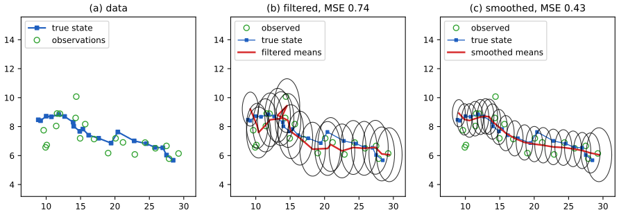
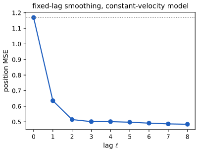
fig_8_2. Reproduces Murphy (2023), Figure 8.2. Download: PDF · SVGHow much lag is enough? Fixed-lag smoothing with lag \(\ell\) reports \(p(\vz_s\given\vy_{1:s+\ell})\). Figure x8.a averages the position error over 200 simulated paths of the same model: one step of hindsight removes about two thirds of the gap between filtering and smoothing, and beyond \(\ell\approx3\) there is nothing left to gain, because the information that \(\vy_{s+k}\) carries about \(\vz_s\) decays geometrically in \(k\).
fig_x8_a. Download: PDF · SVG8.1.2 Bayesian filtering equations
pp. 361–362, (8.4)–(8.7) The Bayes filter updates the belief state recursively, at a cost per step that does not grow with \(t\): the prediction step is the Chapman–Kolmogorov equation and the update step is Bayes' rule,
\[ p(\vz_t\given\vy_{1:t-1})=\int p(\vz_t\given\vz_{t-1})\,p(\vz_{t-1}\given\vy_{1:t-1})\,\d\vz_{t-1}, \tag{8.4} \] \[ p(\vz_t\given\vy_{1:t})=\frac1{Z_t}\,p(\vy_t\given\vz_t)\,p(\vz_t\given\vy_{1:t-1}),\qquad Z_t=\int p(\vy_t\given\vz_t)\,p(\vz_t\given\vy_{1:t-1})\,\d\vz_t=p(\vy_t\given\vy_{1:t-1}), \tag{8.5–8.6} \] \[ \log p(\vy_{1:T})=\sum_{t=1}^T\log p(\vy_t\given\vy_{1:t-1})=\sum_{t=1}^T\log Z_t. \tag{8.7} \]Filling the gap 8.1: the two conditional independences behind the Bayes filter pp. 361–362, (8.4)–(8.7)
The book uses \(p(\vz_t\given\vz_{t-1},\vy_{1:t-1})=p(\vz_t\given\vz_{t-1})\) in (8.4) and \(p(\vy_t\given\vz_t,\vy_{1:t-1})=p(\vy_t\given\vz_t)\) in (8.5) without comment. Both follow from (8.1) alone.
Derivation
Marginals of an initial segment. Integrate (8.1) over \(\vy_T\), then \(\vz_T\), then \(\vy_{T-1}\), and so on, down to the variables \((\vz_{1:t},\vy_{1:t-1})\). At each stage the variable integrated out appears in exactly one remaining factor, a conditional density that integrates to one. Hence
\[ p(\vz_{1:t},\vy_{1:t-1})=p(\vz_1)\prod_{s=2}^tp(\vz_s\given\vz_{s-1})\prod_{s=1}^{t-1}p(\vy_s\given\vz_s),\qquad p(\vz_{1:t},\vy_{1:t})=p(\vz_{1:t},\vy_{1:t-1})\,p(\vy_t\given\vz_t). \](A) \(\vz_t\indep(\vz_{1:t-2},\vy_{1:t-1})\given\vz_{t-1}\). In the first product, \(\vz_t\) appears only in \(p(\vz_t\given\vz_{t-1})\), so dividing by \(p(\vz_{1:t-1},\vy_{1:t-1})\) (the same product without that factor) gives \(p(\vz_t\given\vz_{1:t-1},\vy_{1:t-1})=p(\vz_t\given\vz_{t-1})\). Integrating \(\vz_{1:t-2}\) against \(p(\vz_{1:t-2}\given\vz_{t-1},\vy_{1:t-1})\) leaves \(p(\vz_t\given\vz_{t-1},\vy_{1:t-1})=p(\vz_t\given\vz_{t-1})\), and (8.4) is the law of total probability conditional on \(\vy_{1:t-1}\).
(B) \(\vy_t\indep(\vz_{1:t-1},\vy_{1:t-1})\given\vz_t\). The second identity gives \(p(\vy_t\given\vz_{1:t},\vy_{1:t-1})=p(\vy_t\given\vz_t)\) in the same way, and integrating out \(\vz_{1:t-1}\) gives \(p(\vy_t\given\vz_t,\vy_{1:t-1})=p(\vy_t\given\vz_t)\). Bayes' rule conditional on \(\vy_{1:t-1}\) is then (8.5), and its normaliser is \(\int p(\vy_t,\vz_t\given\vy_{1:t-1})\d\vz_t=p(\vy_t\given\vy_{1:t-1})\), which is (8.6).
(8.7) is the chain rule \(p(\vy_{1:T})=\prod_tp(\vy_t\given\vy_{1:t-1})\) with \(p(\vy_1\given\vy_{1:0})=p(\vy_1)\). For the linear-Gaussian model the code compares this sum of one-step log densities with the log density of the stacked vector \(\vy_{1:T}\) under the full joint Gaussian of (8.1); they agree to \(10^{-10}\). ∎
8.1.3 Bayesian smoothing equations
pp. 362–363, (8.8)–(8.14) Smoothing runs a forward (filtering) pass and then a backward pass from \(t=T\) to \(t=1\) (forwards filtering backwards smoothing). Given \(p(\vz_{t+1}\given\vy_{1:T})\),
\[ p(\vz_t\given\vz_{t+1},\vy_{1:T})=p(\vz_t\given\vz_{t+1},\vy_{1:t})=\frac{p(\vz_{t+1}\given\vz_t)\,p(\vz_t\given\vy_{1:t})}{p(\vz_{t+1}\given\vy_{1:t})}, \tag{8.9–8.11} \] \[ p(\vz_t\given\vy_{1:T})=p(\vz_t\given\vy_{1:t})\int\frac{p(\vz_{t+1}\given\vz_t)\,p(\vz_{t+1}\given\vy_{1:T})}{p(\vz_{t+1}\given\vy_{1:t})}\,\d\vz_{t+1}. \tag{8.13} \]Read (8.14): take the two-slice filtered joint \(p(\vz_t,\vz_{t+1}\given\vy_{1:t})\), divide out the old belief about \(\vz_{t+1}\), multiply in the new one, and integrate \(\vz_{t+1}\) out.
Filling the gap 8.2: why the future data drop out of \(p(\vz_t\given\vz_{t+1},\vy_{1:T})\) p. 362, (8.9)
The first equality of (8.9) is "the Markov property". It says that once \(\vz_{t+1}\) is known, \(\vy_{t+1:T}\) carries no further information about \(\vz_t\).
Derivation
Split (8.1) at time \(t\): \(p(\vz_{1:T},\vy_{1:T})=a(\vz_{1:t},\vy_{1:t})\,p(\vz_{t+1}\given\vz_t)\,b(\vz_{t+1:T},\vy_{t+1:T})\), where \(a\) collects \(p(\vz_1)\), the transitions up to \(t\) and the observations up to \(t\), and \(b\) the transitions after \(t+1\) and the observations after \(t\). Integrating \(\vz_{1:t-1}\) out of \(a\) and \(\vz_{t+2:T}\) out of \(b\),
\[ p(\vz_t,\vz_{t+1},\vy_{1:T})=\tilde a(\vz_t,\vy_{1:t})\,p(\vz_{t+1}\given\vz_t)\,\tilde b(\vz_{t+1},\vy_{t+1:T}). \]As a function of \(\vz_t\) with everything else fixed, this is proportional to \(\tilde a(\vz_t,\vy_{1:t})p(\vz_{t+1}\given\vz_t)\), which does not involve \(\vy_{t+1:T}\). The same function, normalised in \(\vz_t\), is \(p(\vz_t\given\vz_{t+1},\vy_{1:t})\), because \(p(\vz_t,\vz_{t+1},\vy_{1:t})=\tilde a\,p(\vz_{t+1}\given\vz_t)\) (integrate \(\tilde b\) over \(\vy_{t+1:T}\), which gives 1). That is (8.9); (8.10)–(8.11) are Bayes' rule given \(\vy_{1:t}\) with \(p(\vz_{t+1}\given\vz_t,\vy_{1:t})=p(\vz_{t+1}\given\vz_t)\) (Filling the gap 8.1 (A)). Multiplying by \(p(\vz_{t+1}\given\vy_{1:T})\) and integrating \(\vz_{t+1}\) gives (8.12)–(8.14). The division is safe: \(p(\vz_{t+1}\given\vy_{1:T})\propto p(\vz_{t+1}\given\vy_{1:t})p(\vy_{t+1:T}\given\vz_{t+1})\) vanishes wherever the denominator does. ∎
8.1.4 The Gaussian ansatz
p. 363, (8.15) The integrals are tractable in two cases: discrete states (the HMM filter, Section 9.2; on a grid, Section 8.7.1) and linear-Gaussian models (Section 8.2). Otherwise most of the chapter keeps a Gaussian belief for the model with additive Gaussian noise
\[ \vz_t=f(\vz_{t-1},\vu_t)+\N(\mathbf0,\mQ_t),\qquad \vy_t=h(\vz_t,\vu_t)+\N(\mathbf0,\mR_t). \tag{8.15} \]8.2 Inference for linear-Gaussian SSMs
pp. 363–364, (8.16)–(8.19) A linear-Gaussian SSM (LG-SSM, or linear dynamical system) has
\[ p(\vz_t\given\vz_{t-1},\vu_t)=\N(\vz_t\given\mF_t\vz_{t-1}+\mathbf B_t\vu_t+\mathbf b_t,\mQ_t),\qquad p(\vy_t\given\vz_t,\vu_t)=\N(\vy_t\given\mH_t\vz_t+\mathbf D_t\vu_t+\mathbf d_t,\mR_t), \tag{8.16–8.17} \]and without inputs or offsets \(p(\vz_t\given\vz_{t-1})=\N(\mF_t\vz_{t-1},\mQ_t)\), \(p(\vy_t\given\vz_t)=\N(\mH_t\vz_t,\mR_t)\) (8.18)–(8.19). It is a Gaussian Bayes net, so the whole vector \((\vz_{1:T},\vy_{1:T})\) is Gaussian, of dimension \((N_z+N_y)T\) (the book writes \(N_yN_zT\)); the code builds this big Gaussian (joint_gaussian_lgssm) and checks every recursion below against brute-force conditioning. When some state components evolve deterministically, write the noise as \(\mathbf G_t\tilde{\mathbf w}_t\) with a low-dimensional \(\tilde{\mathbf w}_t\), so \(\mQ_t=\mathbf G_t\tilde\mQ_t\mathbf G_t^\T\) is singular; here \(\mathbf G_t\) is \(N_z\times N_q\) (the book's footnote says \(N_y\times N_q\)).
8.2.1 Examples
8.2.1.1 Tracking and state estimation
pp. 364–365, (8.20)–(8.21) With sampling period \(\Delta\), the state \(\vz_t=(x_{t1},x_{t2},\dot x_{t1},\dot x_{t2})\) (position and velocity; the book prints \(\dot x_{t1}\) twice) evolves by the constant-velocity model and the sensor reads the position:
\[ \vz_t=\begin{pmatrix}1&0&\Delta&0\\0&1&0&\Delta\\0&0&1&0\\0&0&0&1\end{pmatrix}\vz_{t-1}+\mathbf q_t,\qquad \vy_t=\begin{pmatrix}1&0&0&0\\0&1&0&0\end{pmatrix}\vz_t+\mathbf r_t. \tag{8.20–8.21} \]Figure 8.2 above is this model. The velocity is never observed; the filter infers it from successive positions through the cross covariance between position and velocity that the prediction step creates.
8.2.1.2 Online Bayesian linear regression (recursive least squares)
p. 365 Take the regression weights as a static state, \(\vz_t=\vw\), with \(p(\vz_t\given\vz_{t-1})=\N(\vz_{t-1},\mathbf0)\) and the time-varying observation \(p(y_t\given\vz_t)=\N(\vx_t^\T\vz_t,\sigma^2)\). The Kalman filter then computes the exact posterior \(p(\vw\given\mathcal D_{1:t})\) one example at a time: recursive least squares, derived in the supplement below.
8.2.1.3 Time series forecasting
p. 365 Structural time-series models are LG-SSMs, and forecasting is (8.2)–(8.3) (book Section 29.12).
Spiral dynamics (supplement 8.1.1)
Supp. pp. 85–86, (S8.1), Figure S8.1 Replace the dynamics by
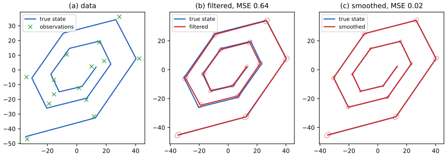
\[ \mF=\begin{pmatrix}0.1&1.1&\Delta&0\\-1&1&0&\Delta\\0&0&0.1&0\\0&0&0&0.1\end{pmatrix}. \tag{S8.1} \]\(\mF\) is block upper triangular, so its eigenvalues are those of the position block \(\begin{pmatrix}0.1&1.1\\-1&1\end{pmatrix}\) (trace 1.1, determinant 1.2, eigenvalues \(0.55\pm1.0548i\)) and \(0.1\) twice. The complex pair makes the motion rotate, and the velocities die out by a factor 10 per step. But the rotating pair has modulus \(\sqrt{1.2}=1.095>1\): each turn multiplies the radius by about 1.095, so the path spirals outwards, not inwards as the supplement says. With the supplement's settings (\(\mQ=0.001\mI\), \(\mR=5\mI\), \(T=15\), start \((8,10,1,0)\)) the noiseless radius grows from 13 to over 200 in 30 steps. Because the motion is nearly deterministic, a few readings pin down the whole path: the smoother's error is 0.016 against 0.644 for the filter.
fig_S8_1. Reproduces Murphy (2023), Supplementary Figure 8.1. Download: PDF · SVG8.2.2 The Kalman filter
pp. 365–370, (8.22)–(8.63), Algorithms 8.1–8.2 The Kalman filter is the Bayes filter for an LG-SSM. The belief state stays Gaussian, \(p(\vz_t\given\vy_{1:t})=\N(\bmu_{t|t},\bSig_{t|t})\), and both steps are closed form.
8.2.2.1 Predict step
\[ \bmu_{t|t-1}=\mF_t\bmu_{t-1|t-1}+\mathbf B_t\vu_t+\mathbf b_t,\qquad \bSig_{t|t-1}=\mF_t\bSig_{t-1|t-1}\mF_t^\T+\mQ_t. \tag{8.22–8.24} \]8.2.2.2 Update step
\[ \hat\vy_t=\mH_t\bmu_{t|t-1}+\mathbf D_t\vu_t+\mathbf d_t,\quad \mS_t=\mH_t\bSig_{t|t-1}\mH_t^\T+\mR_t,\quad \mK_t=\bSig_{t|t-1}\mH_t^\T\mS_t^{-1}, \tag{8.26–8.28} \] \[ \bmu_{t|t}=\bmu_{t|t-1}+\mK_t(\vy_t-\hat\vy_t),\qquad \bSig_{t|t}=\bSig_{t|t-1}-\mK_t\mH_t\bSig_{t|t-1}=\bSig_{t|t-1}-\mK_t\mS_t\mK_t^\T. \tag{8.29–8.31} \]\(\mathbf e_t=\vy_t-\hat\vy_t\) is the innovation, \(\mS_t\) its covariance, \(\mC_t=\bSig_{t|t-1}\mH_t^\T\) the cross covariance of state and observation, and \(\mK_t\) the Kalman gain; in code one solves \(\mK_t\mS_t=\mC_t\) rather than inverting \(\mS_t\). In the scalar case with \(H=1\), \(k_t=\Sigma_{t|t-1}/(\Sigma_{t|t-1}+R_t)\in(0,1)\): the weight given to the reading is the share of the predictive variance that comes from the state, large when the prior is vague or the sensor precise. By the matrix inversion lemma,
\[ \mK_t=\bSig_{t|t-1}\mH_t^\T(\mH_t\bSig_{t|t-1}\mH_t^\T+\mR_t)^{-1}=(\bSig_{t|t-1}^{-1}+\mH_t^\T\mR_t^{-1}\mH_t)^{-1}\mH_t^\T\mR_t^{-1}=\bSig_{t|t}\mH_t^\T\mR_t^{-1}, \tag{8.32} \]the cheaper form when \(N_y\gg N_z\) and \(\mR_t^{-1}\) is known.
8.2.2.3 Posterior predictive
pp. 366–367, (8.33)–(8.36) The one-step predictive density is \(p(\vy_t\given\vy_{1:t-1})=\N(\vy_t\given\hat\vy_t,\mS_t)\) (8.35), and summing its logarithm gives the log likelihood (8.36), the "surprise" of the model at each step. Forecasts \(K\) steps ahead apply the prediction step \(K\) times in latent space and map the result through \(\mH\) once, without sampling observations in between (unlike an RNN).
8.2.2.4 Derivation
pp. 367–368, (8.37)–(8.52) The book derives the filter from the joint Gaussians \(p(\vz_{t-1},\vz_t\given\vy_{1:t-1})\) (8.39)–(8.40) and \(p(\vz_t,\vy_t\given\vy_{1:t-1})\) (8.44)–(8.45). The lower-right block of (8.45) is printed \(\mH_t\bSig_{t|t-1}^{-1}\mH_t^\T+\mR_t\); it is \(\mH_t\bSig_{t|t-1}\mH_t^\T+\mR_t=\mS_t\), as (8.51) and (8.55) have it. Here is the one lemma everything rests on, then the theorem with its proof.
Filling the gap 8.3: the linear Gaussian system, with a proof of the conditioning formula pp. 368–369, (8.53)–(8.56), Algorithm 8.1
Lemma. Let \(\vz\sim\N(\breve{\bmu},\breve{\bSig})\) and \(\vy=\mA\vz+\mathbf b+\boldsymbol\epsilon\) with \(\boldsymbol\epsilon\sim\N(\mathbf0,\boldsymbol\Omega)\) independent of \(\vz\). Then \((\vz,\vy)\) is jointly Gaussian with \(\E\vy=\bmu:=\mA\breve\bmu+\mathbf b\), \(\cov[\vz,\vy]=\mC:=\breve\bSig\mA^\T\), \(\var[\vy]=\mS:=\mA\breve\bSig\mA^\T+\boldsymbol\Omega\) (8.55), and if \(\mS\) is invertible,
\[ \vz\given\vy\sim\N\big(\breve\bmu+\mK(\vy-\bmu),\ \breve\bSig-\mK\mS\mK^\T\big),\qquad \mK=\mC\mS^{-1}. \tag{8.56} \]Proof
\((\vz,\vy)\) is an affine image of the Gaussian vector \((\vz,\boldsymbol\epsilon)\), hence Gaussian, and its moments follow from linearity and the independence of \(\vz\) and \(\boldsymbol\epsilon\). For the conditional, put \(\vw=\vz-\mK\vy\). Then \(\cov[\vw,\vy]=\mC-\mK\mS=\mathbf0\), and since \((\vw,\vy)\) is jointly Gaussian, uncorrelated means independent. So given \(\vy\), \(\vz=\vw+\mK\vy\) has the law of \(\vw\) shifted by \(\mK\vy\): mean \(\E\vw+\mK\vy=\breve\bmu+\mK(\vy-\bmu)\), covariance \(\var[\vw]=\breve\bSig-\mC\mK^\T-\mK\mC^\T+\mK\mS\mK^\T=\breve\bSig-\mK\mS\mK^\T\), using \(\mK\mS=\mC\). The log normaliser returned by Algorithm 8.1 is \(\log\N(\vy\given\bmu,\mS)\), the marginal density of \(\vy\). The same result is proved by completing the square in Result 3.6 of the first volume and in information form in Filling the gap 2.11. ∎
Result 8.1 (the Kalman filter is exact) pp. 365–368, (8.22)–(8.52), Algorithm 8.2
For the LG-SSM (8.16)–(8.17) with \(\vz_0\sim\N(\bmu_{0|0},\bSig_{0|0})\) and \(\mR_t\) positive definite, \(p(\vz_t\given\vy_{1:t})=\N(\bmu_{t|t},\bSig_{t|t})\) and \(p(\vz_t\given\vy_{1:t-1})=\N(\bmu_{t|t-1},\bSig_{t|t-1})\) with the recursions (8.23)–(8.31), and \(p(\vy_t\given\vy_{1:t-1})=\N(\hat\vy_t,\mS_t)\), so (8.36) is the exact log likelihood.
Proof
Induction on \(t\); the case \(t=0\) is the assumption. Predict. Conditionally on \(\vy_{1:t-1}\), \(\vz_{t-1}\sim\N(\bmu_{t-1|t-1},\bSig_{t-1|t-1})\) and \(\vz_t=\mF_t\vz_{t-1}+\mathbf B_t\vu_t+\mathbf b_t+\mathbf q_t\), where \(\mathbf q_t\) is independent of \((\vz_{t-1},\vy_{1:t-1})\) by Filling the gap 8.1 (A). The lemma (marginal of \(\vy\), with \(\vz\to\vz_{t-1}\), \(\vy\to\vz_t\)) gives (8.23)–(8.24). Update. Conditionally on \(\vy_{1:t-1}\), \(\vz_t\sim\N(\bmu_{t|t-1},\bSig_{t|t-1})\) and \(\vy_t=\mH_t\vz_t+\mathbf D_t\vu_t+\mathbf d_t+\mathbf r_t\) with \(\mathbf r_t\) independent of \((\vz_t,\vy_{1:t-1})\) by Filling the gap 8.1 (B). The lemma gives \(p(\vy_t\given\vy_{1:t-1})=\N(\hat\vy_t,\mS_t)\) and, conditioning, (8.29)–(8.31); \(\mS_t\succeq\mR_t\succ0\) is invertible. ∎
Numerically, for a random 3-state, 2-observation model the filtered moments agree with brute-force conditioning of the full joint Gaussian on \(\vy_{1:t}\) to \(10^{-9}\) at every \(t\). The proof in Bishop's notation is Result 13.30 of the companion course.
Filling the gap 8.4: the covariance forms, the Joseph form, and why the update never adds uncertainty pp. 366, 370, (8.30)–(8.32)
The book gives (8.30), (8.31) and (8.32) and mentions numerical problems in Section 8.2.2.6. The three forms are algebraically equal, but only one of them stays positive semidefinite in floating point.
Derivation
Write \(\bSig=\bSig_{t|t-1}\), drop the index \(t\). (8.30) = (8.31). \(\mK\mS\mK^\T=\bSig\mH^\T\mS^{-1}\mS\mK^\T=\bSig\mH^\T\mK^\T=(\mK\mH\bSig)^\T\), and \(\mK\mH\bSig=\bSig\mH^\T\mS^{-1}\mH\bSig\) is symmetric, so \(\mK\mS\mK^\T=\mK\mH\bSig\). Joseph form. For any matrix \(\mK\), the covariance of \(\vz-\bmu-\mK(\vy-\hat\vy)=(\mI-\mK\mH)(\vz-\bmu)-\mK\mathbf r\) is
\[ (\mI-\mK\mH)\bSig(\mI-\mK\mH)^\T+\mK\mR\mK^\T, \]a sum of positive semidefinite terms, and for the Kalman gain it expands to \(\bSig-\mK\mH\bSig-\bSig\mH^\T\mK^\T+\mK\mS\mK^\T=\bSig-\mK\mH\bSig\). In floating point the subtraction in (8.30) can produce a slightly indefinite matrix, while the Joseph form cannot (it is also correct for a suboptimal gain, which is why square-root and ensemble filters are analysed with it). The update never adds uncertainty: \(\bSig_{t|t-1}-\bSig_{t|t}=\mK\mS\mK^\T\succeq0\). (8.32). From \(\mH^\T\mR^{-1}(\mH\bSig\mH^\T+\mR)=(\bSig^{-1}+\mH^\T\mR^{-1}\mH)\bSig\mH^\T\), multiply on the left by \((\bSig^{-1}+\mH^\T\mR^{-1}\mH)^{-1}\) and on the right by \(\mS^{-1}\). The Woodbury identity gives \(\bSig_{t|t}=\bSig-\bSig\mH^\T\mS^{-1}\mH\bSig=(\bSig^{-1}+\mH^\T\mR^{-1}\mH)^{-1}\), the information-form update (8.97), and so \(\mK=\bSig_{t|t}\mH^\T\mR^{-1}\). All of these hold to \(10^{-10}\) in the code. ∎
8.2.2.5 Abstract formulation
pp. 368–369, (8.53)–(8.63) Two functions do all the work, and the same pattern returns for every nonlinear filter in the chapter, with a different way of computing \((\hat\vy,\mS,\mC)\).
Algorithm 8.1 (functions for a linear Gaussian system)
LinGaussJoint\((\breve\bmu,\breve\bSig,\mA,\mathbf b,\boldsymbol\Omega)\): return \(\bmu=\mA\breve\bmu+\mathbf b\), \(\mS=\boldsymbol\Omega+\mA\breve\bSig\mA^\T\), \(\mC=\breve\bSig\mA^\T\).GaussCondition\((\breve\bmu,\breve\bSig,\bmu,\mS,\mC,\vy)\): \(\mK=\mC\mS^{-1}\); return \(\breve\bmu+\mK(\vy-\bmu)\), \(\breve\bSig-\mK\mS\mK^\T\), \(\ell=\log\N(\vy\given\bmu,\mS)\).
Algorithm 8.2 (Kalman filter)
- For \(t=1,\dots,T\): predict \((\bmu_{t|t-1},\bSig_{t|t-1})\) =
LinGaussJoint\((\bmu_{t-1|t-1},\bSig_{t-1|t-1},\mF_t,\mathbf B_t\vu_t+\mathbf b_t,\mQ_t)\); - \((\hat\vy_t,\mS_t,\mC_t)\) =
LinGaussJoint\((\bmu_{t|t-1},\bSig_{t|t-1},\mH_t,\mathbf D_t\vu_t+\mathbf d_t,\mR_t)\); - \((\bmu_{t|t},\bSig_{t|t},\ell_t)\) =
GaussCondition\((\bmu_{t|t-1},\bSig_{t|t-1},\hat\vy_t,\mS_t,\mC_t,\vy_t)\). - Return the filtered moments and \(\sum_t\ell_t\).
Implemented as lin_gauss_joint, gauss_condition and kalman_filter in the code, and in JavaScript in the demonstration, which reproduces the Python numbers to \(10^{-14}\).
8.2.2.6 Numerical issues
p. 370 Remedies: the information filter (Section 8.2.4), square-root filters that propagate a Cholesky or QR factor of \(\bSig_{t|t}\) (so the covariance is positive semidefinite by construction), their combination (the square-root information filter), and QR-based updates without explicit inverses. The Joseph form of Filling the gap 8.4 is the cheapest safeguard.
8.2.2.7 Continuous-time version
p. 370 For linear stochastic differential equations observed continuously, the analogue is the Kalman–Bucy filter, whose covariance obeys a matrix Riccati differential equation.
Derivation of RLS (supplement 8.1.2)
Supp. pp. 85–86, (S8.2)–(S8.14) With \(\mH_t=\vu_t^\T\) (the regressors), \(\mF_t=\mI\), \(\mQ_t=\mathbf0\), \(\mR_t=\sigma^2\), the Kalman filter becomes recursive least squares:
\[ s_t=\vu_t^\T\bSig_{t-1}\vu_t+\sigma^2,\quad \mathbf k_t=\bSig_{t-1}\vu_t/s_t,\quad \bmu_t=\bmu_{t-1}+\mathbf k_t(y_t-\vu_t^\T\bmu_{t-1}),\quad \bSig_t=\bSig_{t-1}-s_t\mathbf k_t\mathbf k_t^\T. \tag{S8.7–S8.12} \]With \(\mathbf V_t=\bSig_t/\sigma^2\) the noise variance cancels from the mean update (S8.13)–(S8.14). The supplement adds that a vague prior \(\bSig_0=\infty\mI\) gives the least-squares estimate.
Filling the gap 8.5: RLS is the batch posterior, and the vague-prior limit is OLS Supp. p. 86
The recursion computes exactly the batch Bayesian linear-regression posterior (first volume, Section 11.7), whatever the order of the data.
Derivation
By Result 8.1 with a static state the filter computes \(p(\vw\given y_{1:t})\) exactly; Bayes' rule with prior \(\N(\bmu_0,\bSig_0)\) and likelihood \(\prod_s\N(y_s\given\vu_s^\T\vw,\sigma^2)\) gives the batch answer \(\bSig_t^{-1}=\bSig_0^{-1}+\sigma^{-2}\mathbf U_t^\T\mathbf U_t\), \(\bmu_t=\bSig_t(\bSig_0^{-1}\bmu_0+\sigma^{-2}\mathbf U_t^\T\vy_{1:t})\), where \(\mathbf U_t\) stacks \(\vu_1^\T,\dots,\vu_t^\T\). In one step this is the rank-one information update \(\bSig_t^{-1}=\bSig_{t-1}^{-1}+\sigma^{-2}\vu_t\vu_t^\T\), whose inverse by the Sherman–Morrison formula is \(\bSig_{t-1}-\bSig_{t-1}\vu_t\vu_t^\T\bSig_{t-1}/s_t\), which is (S8.10). Vague prior. Take \(\bSig_0=c\mI\) and let \(c\to\infty\). If \(\mathbf U_t\) has full column rank, \(\bSig_t=(c^{-1}\mI+\sigma^{-2}\mathbf U_t^\T\mathbf U_t)^{-1}\to\sigma^2(\mathbf U_t^\T\mathbf U_t)^{-1}\) and \(\bmu_t\to(\mathbf U_t^\T\mathbf U_t)^{-1}\mathbf U_t^\T\vy_{1:t}\), the OLS estimate, with posterior standard deviations equal to the usual standard errors (the square roots of the diagonal of \(\sigma^2(\mathbf U^\T\mathbf U)^{-1}\)). Numerically, with \(c=10^8\) the recursion matches OLS to \(10^{-5}\), and with a proper prior it matches the batch posterior to \(10^{-9}\). ∎
Unknown observation noise (supplement 8.1.3)
Supp. p. 87, (S8.15)–(S8.31) For scalar observations with unknown variance \(V=\sigma^2\) (West and Harrison, 1997), scale every covariance by \(V\): \(p(\vz_t\given\vz_{t-1})=\N(\mF_t\vz_{t-1},V\mQ^*_t)\), \(p(y_t\given\vz_t)=\N(\mathbf h_t^\T\vz_t,V)\), with prior \(\lambda=1/V\sim\Ga(\nu_0/2,\nu_0\tau_0/2)\) and \(\vz\given\lambda\sim\N(\bmu_0,V\bSig^*_0)\). The belief state stays normal-gamma, and the filter is the Kalman filter on the starred (unscaled) covariances plus two scalar updates:
\[ e_t=y_t-\mathbf h_t^\T\bmu_{t|t-1},\quad s^*_t=\mathbf h_t^\T\bSig^*_{t|t-1}\mathbf h_t+1,\quad \mathbf k_t=\bSig^*_{t|t-1}\mathbf h_t/s^*_t,\quad \nu_t=\nu_{t-1}+1,\quad \nu_t\tau_t=\nu_{t-1}\tau_{t-1}+e_t^2/s^*_t, \tag{S8.23–S8.29} \]with \(\bSig^*_{t|t-1}=\mF_t\bSig^*_{t-1}\mF_t^\T+\mQ^*_t\) (the supplement drops the transpose), \(\bmu_t=\bmu_{t|t-1}+\mathbf k_te_t\) (the supplement writes \(\bmu_{t-1}\)), \(\bSig^*_t=\bSig^*_{t|t-1}-s^*_t\mathbf k_t\mathbf k_t^\T\). Integrating \(V\) out, \(p(\vz_t\given\mathcal D_{1:t})\) is Student \(\mathcal T_{\nu_t}(\bmu_t,\tau_t\bSig^*_t)\) and the predictive is \(\mathcal T_{\nu_{t-1}}(y_t\given\mathbf h_t^\T\bmu_{t|t-1},\tau_{t-1}s^*_t)\) (S8.30)–(S8.31).
Filling the gap 8.6: the normal-gamma filter Supp. p. 87
The supplement states the recursions; here is why the belief stays normal-gamma and why \(\nu\tau\) accumulates squared standardised innovations.
Derivation
Suppose \(\vz_{t-1}\given\lambda,\mathcal D_{1:t-1}\sim\N(\bmu_{t-1},\lambda^{-1}\bSig^*_{t-1})\) and \(\lambda\given\mathcal D_{1:t-1}\sim\Ga(\nu_{t-1}/2,\nu_{t-1}\tau_{t-1}/2)\). Given \(\lambda\) everything is linear-Gaussian with every covariance multiplied by \(\lambda^{-1}\), so Result 8.1 applies with \(\bSig=\lambda^{-1}\bSig^*\): the gain \(\mathbf k_t=\lambda^{-1}\bSig^*\mathbf h/(\lambda^{-1}s^*_t)\) does not depend on \(\lambda\), the posterior is \(\N(\bmu_t,\lambda^{-1}\bSig^*_t)\) with the starred recursions, and \(p(y_t\given\lambda,\mathcal D_{1:t-1})=\N(e_t\given0,\lambda^{-1}s^*_t)\propto\lambda^{1/2}\exp(-\lambda e_t^2/(2s^*_t))\). Update of \(\lambda\): multiplying the gamma density by this likelihood adds \(1/2\) to the shape and \(e_t^2/(2s^*_t)\) to the rate, which is (S8.28)–(S8.29). Marginals: a normal with precision scaled by a gamma variable integrates to a Student distribution (Filling the gap 2.3): \(\nu\) degrees of freedom and scale \(\tau\) times the starred covariance. For a static regression (\(\mF=\mI\), \(\mQ^*=\mathbf0\)) the code confirms that the final \((\bmu,\bSig^*,\nu,\nu\tau)\) equal the batch normal-inverse-gamma posterior and that the sum of the Student log predictive densities equals the batch marginal likelihood (a multivariate Student density) to \(10^{-8}\). ∎
Predictive coding as Kalman filtering (supplement 8.1.4)
Supp. pp. 88–89, (S8.32)–(S8.46) Predictive coding is a theory in which the brain minimises precision-weighted prediction errors. For an LG-SSM with a Gaussian belief \(q(\vz_t)=\N(\bmu_t,\cdot)\) whose covariance comes from the Hessian (a Laplace approximation), the free energy reduces to the negative log joint at the mean,
\[ \mathcal F_t(\bmu_t)=\tfrac12\boldsymbol\epsilon_y^\T\bSig_y^{-1}\boldsymbol\epsilon_y+\tfrac12\boldsymbol\epsilon_z^\T\bSig_z^{-1}\boldsymbol\epsilon_z+\const,\qquad \boldsymbol\epsilon_y=\vy_t-\mH\bmu_t,\quad \boldsymbol\epsilon_z=\bmu_t-\mF\bmu_{t-1}-\mathbf B\vu_{t-1}, \]with gradient \(\nabla\mathcal F_t=-\mH^\T\bSig_y^{-1}\boldsymbol\epsilon_y+\bSig_z^{-1}\boldsymbol\epsilon_z\) (S8.46). The supplement's intermediate lines (S8.34)–(S8.44) differentiate \(p\) instead of \(\log p\), drop the factor \(\tfrac12\) of the second-order term, write the objective as \(+\log p\) while minimising it, and misplace a transpose; the end result (S8.45)–(S8.46) is right.
Filling the gap 8.7: predictive coding converges to the Kalman mean, and the parameter gradients Supp. pp. 88–89
The supplement asserts that the result is "exact for this model class". Precisely: with the previous estimate treated as known (the factorised approximation), the minimiser of \(\mathcal F_t\) is the Kalman update started from a point mass at \(\bmu_{t-1}\).
Derivation
\(\mathcal F_t\) is a convex quadratic with Hessian \(\mH^\T\bSig_y^{-1}\mH+\bSig_z^{-1}\succ0\), so gradient descent with a small enough step converges to the unique zero of (S8.46): \(\bmu^*=(\bSig_z^{-1}+\mH^\T\bSig_y^{-1}\mH)^{-1}(\bSig_z^{-1}\bmu_{t|t-1}+\mH^\T\bSig_y^{-1}\vy_t)\) with \(\bmu_{t|t-1}=\mF\bmu_{t-1}+\mathbf B\vu_{t-1}\). This is the information form of the Kalman update with prior covariance \(\bSig_z\) (Filling the gap 8.4), and the Laplace covariance, the inverse Hessian, is the Kalman posterior covariance. A full Kalman filter would use \(\mF\bSig_{t-1|t-1}\mF^\T+\bSig_z\) as prior covariance; the factorised approximation drops the first term. In the code 20,000 gradient steps reach the Kalman mean to \(10^{-8}\). Parameter gradients. Differentiating \(\mathcal F_t\): \(\partial\mathcal F_t/\partial\mF=-\bSig_z^{-1}\boldsymbol\epsilon_z\bmu_{t-1}^\T\), \(\partial\mathcal F_t/\partial\mathbf B=-\bSig_z^{-1}\boldsymbol\epsilon_z\vu_{t-1}^\T\), \(\partial\mathcal F_t/\partial\mH=-\bSig_y^{-1}\boldsymbol\epsilon_y\bmu_t^\T\) (confirmed by finite differences). The supplement prints \(-\bSig_z\boldsymbol\epsilon_y\bmu_{t-1}^\T\) for the first two (wrong error term and a covariance where a precision belongs) and \(-\bSig_y\boldsymbol\epsilon_y\bmu_t^\T\) for the third. Each is a product of a prediction error and an activity: a Hebbian rule. ∎
8.2.3 The Kalman (RTS) smoother
pp. 370–371, (8.64)–(8.84) The Rauch–Tung–Striebel smoother runs backwards over the filtered moments, without touching the observations again:
\[ \bmu_{t+1|t}=\mF_{t+1}\bmu_{t|t},\quad \bSig_{t+1|t}=\mF_{t+1}\bSig_{t|t}\mF_{t+1}^\T+\mQ_{t+1},\quad \mJ_t=\bSig_{t|t}\mF_{t+1}^\T\bSig_{t+1|t}^{-1}, \tag{8.65–8.67} \] \[ \bmu_{t|T}=\bmu_{t|t}+\mJ_t(\bmu_{t+1|T}-\bmu_{t+1|t}),\qquad \bSig_{t|T}=\bSig_{t|t}+\mJ_t(\bSig_{t+1|T}-\bSig_{t+1|t})\mJ_t^\T. \tag{8.68–8.69} \](The book writes \(\mF_t\) in (8.65)–(8.67) and \(\mQ_{t+1}\) in (8.66); the step from \(t\) to \(t+1\) uses \(\mF_{t+1}\) and \(\mQ_{t+1}\) in the convention (8.16), and with time-invariant matrices the distinction disappears.)
Result 8.2 (the RTS smoother, with the lag-one cross covariance) pp. 370–371, (8.64)–(8.84)
For the LG-SSM with \(\bSig_{t+1|t}\) invertible, \(p(\vz_t\given\vy_{1:T})=\N(\bmu_{t|T},\bSig_{t|T})\) with (8.65)–(8.69), and \(\cov[\vz_t,\vz_{t+1}\given\vy_{1:T}]=\mJ_t\bSig_{t+1|T}\).
Proof
Backward induction from \(t=T\), where the smoothed and filtered moments coincide. Given \(\vy_{1:t}\), \(\vz_t\sim\N(\bmu_{t|t},\bSig_{t|t})\) and \(\vz_{t+1}=\mF_{t+1}\vz_t+\mathbf q_{t+1}\), so by the lemma of Filling the gap 8.3, \((\vz_t,\vz_{t+1})\) is jointly Gaussian with cross covariance \(\bSig_{t|t}\mF_{t+1}^\T\) (8.72), and conditioning on \(\vz_{t+1}\) gives
\[ \vz_t\given\vz_{t+1},\vy_{1:t}\sim\N\big(\bmu_{t|t}+\mJ_t(\vz_{t+1}-\bmu_{t+1|t}),\ \bSig_{t|t}-\mJ_t\bSig_{t+1|t}\mJ_t^\T\big). \tag{8.78–8.79} \]By Filling the gap 8.2 this is also the law of \(\vz_t\) given \(\vz_{t+1}\) and \(\vy_{1:T}\). So, given \(\vy_{1:T}\), \(\vz_t=\bmu_{t|t}+\mJ_t(\vz_{t+1}-\bmu_{t+1|t})+\mathbf w\) with \(\mathbf w\sim\N(\mathbf0,\mathbf V_2)\) independent of \(\vz_{t+1}\sim\N(\bmu_{t+1|T},\bSig_{t+1|T})\). Taking moments: the mean is (8.68); the covariance is \(\mJ_t\bSig_{t+1|T}\mJ_t^\T+\bSig_{t|t}-\mJ_t\bSig_{t+1|t}\mJ_t^\T\), which is (8.69); and \(\cov[\vz_t,\vz_{t+1}\given\vy_{1:T}]=\mJ_t\bSig_{t+1|T}\). ∎
The cross covariance is what the E step of EM needs (Result 13.34 of the companion course). In the code all three match brute-force conditioning of the joint Gaussian to \(10^{-9}\).
8.2.3.3 Two-filter smoothing
p. 372 Instead of the RTS recursion, combine the forward filter with a backward pass that computes \(p(\vy_{t+1:T}\given\vz_t)\). That function is a likelihood in \(\vz_t\), not a density, and at \(t=T\) it is constant ("\(\bSig^b_T=\infty\mI\)"), which is a problem in moment form and none in information form.
Filling the gap 8.8: the backward information filter p. 372
The book does not give the backward recursion. In information form it starts from zero precision and needs no infinite covariance.
Derivation
Let \(\beta_t(\vz)=p(\vy_{t+1:T}\given\vz_t=\vz)\propto\exp(-\tfrac12\vz^\T\bLam^b_t\vz+(\beta^b_t)^\T\vz)\), with \(\bLam^b_T=\mathbf0\), \(\beta^b_T=\mathbf0\) (no evidence beyond \(T\)). Combine. As in Filling the gap 8.2, \(\vy_{t+1:T}\indep\vy_{1:t}\given\vz_t\), so \(p(\vz_t\given\vy_{1:T})\propto p(\vz_t\given\vy_{1:t})\beta_t(\vz_t)\): precision \(\bSig_{t|t}^{-1}+\bLam^b_t\), information vector \(\bSig_{t|t}^{-1}\bmu_{t|t}+\beta^b_t\). Absorb \(\vy_t\). \(p(\vy_t\given\vz_t)\beta_t(\vz_t)\) has precision \(\bLam_t'=\bLam^b_t+\mH_t^\T\mR_t^{-1}\mH_t\) and information \(\beta'_t=\beta^b_t+\mH_t^\T\mR_t^{-1}\vy_t\). Step back. \(\beta_{t-1}(\vz)=\int\N(\vz_t\given\mF_t\vz,\mQ_t)\,p(\vy_t\given\vz_t)\beta_t(\vz_t)\,\d\vz_t\). The exponent is \(-\tfrac12\vz_t^\T(\mQ_t^{-1}+\bLam'_t)\vz_t+\vz_t^\T(\mQ_t^{-1}\mF_t\vz+\beta'_t)-\tfrac12\vz^\T\mF_t^\T\mQ_t^{-1}\mF_t\vz\); integrating out \(\vz_t\) (with \(\mathbf G=(\mQ_t^{-1}+\bLam'_t)^{-1}\)) leaves
\[ \bLam^b_{t-1}=\mF_t^\T(\mQ_t^{-1}-\mQ_t^{-1}\mathbf G\mQ_t^{-1})\mF_t,\qquad \beta^b_{t-1}=\mF_t^\T\mQ_t^{-1}\mathbf G\beta'_t. \]When \(\bLam'_t\) is invertible the first is \(\mF_t^\T(\mQ_t+\bLam_t'^{-1})^{-1}\mF_t\) by Woodbury: the backward "covariance" grows by \(\mQ_t\) when stepping back, mirroring (8.24). The code's two_filter_smoother reproduces the RTS moments to \(10^{-8}\) on a time-varying model. ∎
The book prefers the RTS form: it is more stable and generalises directly to the nonlinear smoothers of Sections 8.3.3 and 8.4.3.
8.2.3.4 Time and space complexity
p. 372 Each step costs \(O(N_z^3)\) for \(\mF\bSig\mF^\T\) and the inverse in \(\mJ_t\), plus \(O(N_z^2N_y+N_y^3)\) for the update, so the total is \(O(T(N_z^3+N_z^2N_y+N_y^3))\), as Section 8.2 says (\(O(TN_z^3)\) for fixed \(N_y\)); the per-step count printed in Section 8.2.3.4, \(O(N_y^3+N_z^2+N_yN_z)\), is too small. A parallel prefix scan brings the depth down to \(O(\log T)\) on parallel hardware (Särkkä and García-Fernández, 2021).
8.2.3.5 Forwards filtering backwards sampling
p. 372, (8.85)–(8.88) To draw whole paths from \(p(\vz_{1:T}\given\vy_{1:T})\): sample \(\vz_T\sim\N(\bmu_{T|T},\bSig_{T|T})\), then for \(t=T-1,\dots,1\)
\[ \vz_t\sim\N\big(\bmu_{t|t}+\mJ_t(\vz_{t+1}-\mF_{t+1}\bmu_{t|t}),\ \bSig_{t|t}-\mJ_t\bSig_{t+1|t}\mJ_t^\T\big),\qquad \bSig_{t|t}-\mJ_t\bSig_{t+1|t}\mJ_t^\T=\bSig_{t|t}(\mI-\mF_{t+1}^\T\mJ_t^\T). \tag{8.85–8.88} \]Filling the gap 8.9: why backward sampling gives exact joint draws p. 372
(8.85) is the conditional of one state given the next; the book does not say why chaining these conditionals samples the joint.
Derivation
By the chain rule, \(p(\vz_{1:T}\given\vy_{1:T})=p(\vz_T\given\vy_{1:T})\prod_{t=1}^{T-1}p(\vz_t\given\vz_{t+1:T},\vy_{1:T})\). The argument of Filling the gap 8.2, with \(b\) now also depending on \(\vz_{t+2:T}\), shows \(p(\vz_t\given\vz_{t+1:T},\vy_{1:T})=p(\vz_t\given\vz_{t+1},\vy_{1:t})\): given the next state, neither the later states nor the later data matter. That conditional is (8.78)–(8.79), i.e. (8.85)–(8.87). The last identity in (8.88): \(\mJ_t\bSig_{t+1|t}\mJ_t^\T=\bSig_{t|t}\mF_{t+1}^\T\bSig_{t+1|t}^{-1}\bSig_{t+1|t}\mJ_t^\T=\bSig_{t|t}\mF_{t+1}^\T\mJ_t^\T\). With 40,000 draws the sample means, covariances and lag-one cross covariances match the smoother of Result 8.2 to Monte Carlo accuracy. FFBS is the building block of blocked Gibbs samplers for SSM parameters (Section 8.7.4). ∎
8.2.4 Information form filtering and smoothing
pp. 372–375, (8.89)–(8.123) In information form, conditioning is easy (add precisions) and marginalising is hard (a Schur complement), the reverse of moment form. Write \(p(\vz_t\given\vy_{1:s})=\Nc(\beta_{t|s},\bLam_{t|s})\). Predict (8.89)–(8.95), with \(\mathbf b'_t=\mathbf B_t\vu_t+\mathbf b_t\):
\[ \mathbf M_t=\bLam_{t-1|t-1}+\mF_t^\T\mQ_t^{-1}\mF_t,\quad \mJ_t=\mQ_t^{-1}\mF_t\mathbf M_t^{-1},\quad \bLam_{t|t-1}=\mQ_t^{-1}-\mJ_t\mathbf M_t\mJ_t^\T,\quad \beta_{t|t-1}=\mJ_t\beta_{t-1|t-1}+\bLam_{t|t-1}\mathbf b'_t. \]Update (8.96)–(8.98): \(\bLam_{t|t}=\bLam_{t|t-1}+\mH_t^\T\mR_t^{-1}\mH_t\), \(\beta_{t|t}=\beta_{t|t-1}+\mH_t^\T\mR_t^{-1}(\vy_t-\mathbf D_t\vu_t-\mathbf d_t)\). Smooth (8.110)–(8.115), written here with the indices of the step \(t\to t+1\) and the offset terms that the book leaves out:
\[ \mathbf U_t=\mQ_{t+1}^{-1}+\bLam_{t+1|T}-\bLam_{t+1|t},\quad \mL_t=\mF_{t+1}^\T\mQ_{t+1}^{-1}\mathbf U_t^{-1},\quad \bLam_{t|T}=\bLam_{t|t}+\mF_{t+1}^\T\mQ_{t+1}^{-1}\mF_{t+1}-\mL_t\mathbf U_t\mL_t^\T, \] \[ \beta_{t|T}=\beta_{t|t}-\mF_{t+1}^\T\mQ_{t+1}^{-1}\mathbf b'_{t+1}+\mL_t\big(\mQ_{t+1}^{-1}\mathbf b'_{t+1}+\beta_{t+1|T}-\beta_{t+1|t}\big). \]Filling the gap 8.10: deriving the information filter and smoother, and two corrections pp. 373–375, (8.99)–(8.123)
The book derives both by "the marginalisation formulae"; here they are carried out. They expose two problems in the printed smoother: (8.111)–(8.114) use \(\mF_t,\mQ_t\) where the step from \(t\) to \(t+1\) needs \(\mF_{t+1},\mQ_{t+1}\) (as (8.120) itself has; (8.113) also has a bare \(\mF\)), and (8.115) is correct only without inputs or offsets.
Derivation
Marginalisation in information form. If \((\vx_1,\vx_2)\sim\Nc\big((\beta_1,\beta_2),[\bLam_{11},\bLam_{12};\bLam_{21},\bLam_{22}]\big)\) then \(\vx_2\sim\Nc(\beta_2-\bLam_{21}\bLam_{11}^{-1}\beta_1,\ \bLam_{22}-\bLam_{21}\bLam_{11}^{-1}\bLam_{12})\): complete the square in \(\vx_1\) and integrate it out (Filling the gap 2.10). Predict. The joint of \((\vz_{t-1},\vz_t)\) given \(\vy_{1:t-1}\) is the product \(\Nc(\vz_{t-1}\given\beta_{t-1|t-1},\bLam_{t-1|t-1})\N(\vz_t\given\mF_t\vz_{t-1}+\mathbf b',\mQ_t)\); expanding the second exponent gives (8.103)–(8.104): \(\bLam_{11}=\mathbf M_t\), \(\bLam_{12}=-\mF_t^\T\mQ_t^{-1}\), \(\bLam_{22}=\mQ_t^{-1}\), \(\beta_1=\beta_{t-1|t-1}-\mF_t^\T\mQ_t^{-1}\mathbf b'\), \(\beta_2=\mQ_t^{-1}\mathbf b'\). Marginalising \(\vz_{t-1}\): \(\bLam_{t|t-1}=\mQ_t^{-1}-\mQ_t^{-1}\mF_t\mathbf M_t^{-1}\mF_t^\T\mQ_t^{-1}=\mQ_t^{-1}-\mJ_t\mathbf M_t\mJ_t^\T\) (8.92)–(8.94), and
\[ \beta_{t|t-1}=\mQ_t^{-1}\mathbf b'+\mJ_t(\beta_{t-1|t-1}-\mF_t^\T\mQ_t^{-1}\mathbf b')=\mJ_t\beta_{t-1|t-1}+(\mQ_t^{-1}-\mJ_t\mF_t^\T\mQ_t^{-1})\mathbf b'=\mJ_t\beta_{t-1|t-1}+\bLam_{t|t-1}\mathbf b', \]which is (8.95). By Woodbury, \(\bLam_{t|t-1}=(\mQ_t+\mF_t\bSig_{t-1|t-1}\mF_t^\T)^{-1}\), the inverse of (8.24). Update. Multiply by \(\N(\vy_t\given\mH_t\vz_t+\mathbf d',\mR_t)\) as a function of \(\vz_t\): it adds \(\mH_t^\T\mR_t^{-1}\mH_t\) to the precision and \(\mH_t^\T\mR_t^{-1}(\vy_t-\mathbf d')\) to the information vector, (8.97)–(8.98). Smooth. By (8.14), \(p(\vz_t\given\vy_{1:T})=\int p(\vz_t,\vz_{t+1}\given\vy_{1:t})\,p(\vz_{t+1}\given\vy_{1:T})/p(\vz_{t+1}\given\vy_{1:t})\,\d\vz_{t+1}\). The two-slice joint has the blocks above with \(t-1\to t\), \(t\to t+1\), so it involves \(\mF_{t+1},\mQ_{t+1},\mathbf b'_{t+1}\); the ratio adds \(\bLam_{t+1|T}-\bLam_{t+1|t}\) to the \((2,2)\) block and \(\beta_{t+1|T}-\beta_{t+1|t}\) to \(\beta_2\). Marginalising \(\vz_{t+1}\) now (the roles of the blocks swap) gives \(\bLam_{t|T}=\bLam_{t|t}+\mF_{t+1}^\T\mQ_{t+1}^{-1}\mF_{t+1}-\mF_{t+1}^\T\mQ_{t+1}^{-1}\mathbf U_t^{-1}\mQ_{t+1}^{-1}\mF_{t+1}\), and the information vector displayed above, in which \(\beta_1\) and \(\beta_2\) carry the offset terms. The book's (8.120) sets \(\beta_{t,t+1|t}=(\beta_{t|t},\mathbf0)\), which is the joint only when \(\mathbf b'_{t+1}=\mathbf0\).
Numerical confirmation. On a random time-varying model with inputs, the information filter equals the moment filter to \(10^{-9}\); the smoother above equals the RTS smoother to \(10^{-8}\); the printed indexing (\(\mF_t,\mQ_t\)) is off by 0.36 in the first smoothed covariance, and omitting the offset terms shifts the smoothed means. Without offsets and with time-invariant matrices, (8.110)–(8.115) as printed are correct. ∎
8.3 Inference based on local linearization
p. 375 For the nonlinear model (8.15), linearise \(f\) and \(h\) around the current estimate by a first-order Taylor expansion and apply the Kalman filter to the linearised, time-varying model: the extended Kalman filter (EKF).
8.3.1 Taylor series expansion
pp. 375–376, (8.124)–(8.135), Algorithm 8.3 If \(\vx\sim\N(\bmu,\bSig)\) and \(g\) is a diffeomorphism, the exact density of \(\vy=g(\vx)\) is \(p(\vy)=|\det\Jac(g^{-1})(\vy)|\,\N(g^{-1}(\vy)\given\bmu,\bSig)\) (8.124), rarely Gaussian. With \(g(\bmu+\boldsymbol\delta)\approx g(\bmu)+\mathbf G\boldsymbol\delta\), \(\mathbf G=\Jac(g)(\bmu)\), the approximation is \(\E\vy\approx g(\bmu)\), \(\cov\vy\approx\mathbf G\bSig\mathbf G^\T\) (8.127)–(8.133); for \(\vy=g(\vx)+\mathbf q\), \(\mathbf q\sim\N(\mathbf 0,\boldsymbol\Omega)\), Algorithm 8.3 returns \(\hat\vy=g(\bmu)\), \(\mS=\mathbf G\bSig\mathbf G^\T+\boldsymbol\Omega\), \(\mC=\bSig\mathbf G^\T\) (8.135).
Filling the gap 8.11: what linearisation misses, exactly, for a quadratic map pp. 375–377
The book says the EKF does poorly when the prior is broad or the map strongly curved, and mentions the second-order EKF. A quadratic map shows the size of the error.
Derivation
Let \(g(\vx)=\vx^\T\mA\vx\) with \(\mA\) symmetric, \(\vx=\bmu+\boldsymbol\delta\), \(\boldsymbol\delta\sim\N(\mathbf0,\bSig)\). Then \(g=\bmu^\T\mA\bmu+2\bmu^\T\mA\boldsymbol\delta+\boldsymbol\delta^\T\mA\boldsymbol\delta\). Since \(\E\boldsymbol\delta^\T\mA\boldsymbol\delta=\Tr(\mA\bSig)\), \(\var(\boldsymbol\delta^\T\mA\boldsymbol\delta)=2\Tr(\mA\bSig\mA\bSig)\) (Gaussian quadratic forms) and the linear and quadratic parts are uncorrelated (their product has only odd moments of \(\boldsymbol\delta\)),
\[ \E g=\bmu^\T\mA\bmu+\Tr(\mA\bSig),\qquad \var g=4\bmu^\T\mA\bSig\mA\bmu+2\Tr\big((\mA\bSig)^2\big). \]The Taylor transform (gradient \(\mathbf G=2\bmu^\T\mA\)) gives \(\bmu^\T\mA\bmu\) and \(4\bmu^\T\mA\bSig\mA\bmu\): it misses \(\Tr(\mA\bSig)\) in the mean and \(2\Tr((\mA\bSig)^2)\) in the variance. Both errors grow with the spread \(\bSig\) (linearly and quadratically) and with the curvature \(\mA\), the two failure modes the book names. The second-order EKF adds exactly these terms, \(\tfrac12\Tr(\nabla^2g_i\,\bSig)\) to each mean component and \(\tfrac12\Tr(\nabla^2g_i\bSig\nabla^2g_j\bSig)\) to each covariance entry. A Gauss–Hermite rule of order 3 gets both moments exactly (Filling the gap 8.18). ∎
8.3.2 The extended Kalman filter (EKF)
pp. 376–379, (8.136)–(8.147), Algorithm 8.4, Figure 8.4 One step of the EKF linearises the dynamics at \(\bmu_{t-1|t-1}\) and the observation model at \(\bmu_{t|t-1}\):
\[ \bmu_{t|t-1}=f(\bmu_{t-1|t-1},\vu_t),\quad \bSig_{t|t-1}=\mF_t\bSig_{t-1|t-1}\mF_t^\T+\mQ_t,\quad \mF_t=\Jac(f(\cdot,\vu_t))(\bmu_{t-1|t-1}), \tag{8.139–8.140} \] \[ \hat\vy_t=h(\bmu_{t|t-1},\vu_t),\quad \mH_t=\Jac(h(\cdot,\vu_t))(\bmu_{t|t-1}), \tag{8.141–8.145} \]followed by (8.142)–(8.145), identical to (8.27)–(8.31). The book defines \(\mF_t\) as the Jacobian at \(\bmu_{t|t-1}\); it must be taken at \(\bmu_{t-1|t-1}\), the point around which \(f\) is expanded (as in (8.136) and in (S8.65) of the supplement).
Filling the gap 8.12: the EKF is the exact Kalman filter of a linearised model (supplement 8.2.1) Supp. pp. 89–90, (S8.47)–(S8.55)
The supplement's derivation forms the two joint Gaussians with the linearisations. A shorter way to see it, which also fixes which point each Jacobian belongs to:
Derivation
At step \(t\), replace \(f\) by its tangent \(\tilde f(\vz)=f(\bmu_{t-1|t-1})+\mF_t(\vz-\bmu_{t-1|t-1})\) and, after predicting, \(h\) by \(\tilde h(\vz)=h(\bmu_{t|t-1})+\mH_t(\vz-\bmu_{t|t-1})\). These are affine maps, so Result 8.1 applies to the linear-Gaussian model with offsets \(\mathbf b'=f(\bmu_{t-1|t-1})-\mF_t\bmu_{t-1|t-1}\) and \(\mathbf d'=h(\bmu_{t|t-1})-\mH_t\bmu_{t|t-1}\): the predicted mean is \(\mF_t\bmu_{t-1|t-1}+\mathbf b'=f(\bmu_{t-1|t-1})\) and the predicted observation \(\mH_t\bmu_{t|t-1}+\mathbf d'=h(\bmu_{t|t-1})\), which are (8.139) and (8.141); the covariances and gain are those of the linear filter. The approximation is entirely in replacing \(f,h\) by tangents at the current means. Consequently the EKF on a linear model is the Kalman filter (confirmed to \(10^{-10}\)), and \(\mQ\), \(\mR\) carry the index of the step being taken (the supplement's \(\mQ_{t-1}\), \(\mR_{t-1}\) in (S8.49), (S8.52) are slips). ∎
8.3.2.1 Accuracy
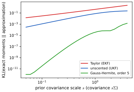
p. 377 The EKF degrades when the prior covariance is large (mass far from the expansion point) or the map is strongly nonlinear near the mean. Figure x8.b measures this for the map of Figure 8.5: the KL divergence from the exact moment-matched Gaussian to the Taylor approximation grows steadily with the prior scale, and stays one to two orders of magnitude above the unscented one.
fig_x8_b. Download: PDF · SVG8.3.2.2 Iterated EKF
pp. 377–378, (8.146), Algorithm 8.4 The iterated EKF relinearises the observation model around the latest posterior mean rather than the prior mean, and is a Gauss–Newton method for the MAP estimate of
\[ \mathcal L(\vz_t)=\tfrac12(\vy_t-h(\vz_t))^\T\mR_t^{-1}(\vy_t-h(\vz_t))+\tfrac12(\vz_t-\bmu_{t|t-1})^\T\bSig_{t|t-1}^{-1}(\vz_t-\bmu_{t|t-1}). \tag{8.146} \]Filling the gap 8.13: the iterated EKF is Gauss–Newton, and Algorithm 8.4 as printed is not pp. 377–378
The book cites the Gauss–Newton interpretation. Deriving it shows what each iteration must compute.
Derivation
Write \(\bmu=\bmu_{t|t-1}\), \(\bSig=\bSig_{t|t-1}\), and \(\mathcal L=\tfrac12\|\mathbf r(\vz)\|^2\) with residual \(\mathbf r=(\mR^{-1/2}(\vy-h(\vz)),\ \bSig^{-1/2}(\vz-\bmu))\) and Jacobian \(\mathbf J_r=(-\mR^{-1/2}\mH_j,\ \bSig^{-1/2})\), \(\mH_j=\Jac(h)(\vz_j)\). The Gauss–Newton step \(\vz_{j+1}=\vz_j-(\mathbf J_r^\T\mathbf J_r)^{-1}\mathbf J_r^\T\mathbf r\) has \(\mathbf J_r^\T\mathbf J_r=\bSig^{-1}+\mH_j^\T\mR^{-1}\mH_j=:\mathbf P^{-1}\), so
\[ \vz_{j+1}=\vz_j+\mathbf P\big[\mH_j^\T\mR^{-1}(\vy-h(\vz_j))-\bSig^{-1}(\vz_j-\bmu)\big]=\bmu+\mK_j\big[\vy-h(\vz_j)-\mH_j(\bmu-\vz_j)\big], \]using \(\mI-\mathbf P\bSig^{-1}=\mathbf P\mH_j^\T\mR^{-1}\mH_j\) and \(\mK_j=\mathbf P\mH_j^\T\mR^{-1}=\bSig\mH_j^\T(\mH_j\bSig\mH_j^\T+\mR)^{-1}\) (8.32). So each iteration is a Kalman update of the prior \((\bmu,\bSig)\), with \(\mS=\mH_j\bSig\mH_j^\T+\mR\), \(\mC=\bSig\mH_j^\T\), and predicted observation \(h(\vz_j)+\mH_j(\bmu-\vz_j)\), the tangent at \(\vz_j\) evaluated at the prior mean. With \(\vz_1=\bmu\) one iteration is the EKF, and a fixed point is a stationary point of (8.146). Algorithm 8.4 instead calls LinearizedGaussJoint at \((\bmu_{t|t},\bSig_{t|t})\): it builds \(\mS,\mC\) from the posterior covariance and uses \(\hat\vy=h(\bmu_{t|t})\) without the correction \(\mH_j(\bmu-\vz_j)\). For a range-bearing observation the code finds that 30 Gauss–Newton iterations reach the MAP to \(10^{-6}\), while iterating Algorithm 8.4 literally settles at a different point, (3.107, 1.215) against the MAP (3.271, 1.459). ∎
Gauss–Newton can diverge; damped versions use line search or Levenberg–Marquardt.
8.3.2.3 Example: tracking a point spiraling in 2d
pp. 378–379, (8.147), Figure 8.4 Dynamics \(f(\vz)=(z_1+\Delta\sin z_2,\ z_2+\Delta\cos z_1)\) (8.147), full but noisy observation \(h(\vz)=\vz\). Exact inference is intractable even here.
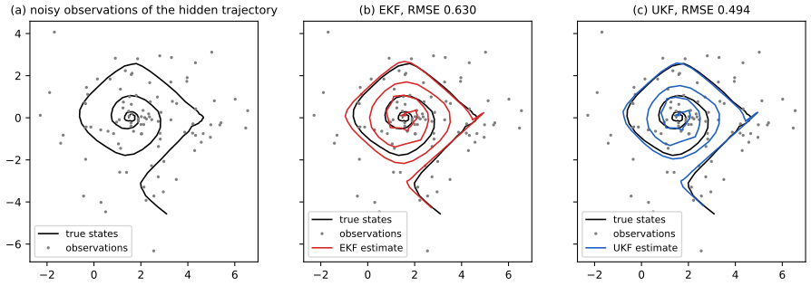
fig_8_4. Reproduces Murphy (2023), Figure 8.4. Download: PDF · SVG8.3.2.4 Example: neural network training
p. 379 Treating the weights of an MLP as the state, the EKF trains the network online (book Section 17.5.2); the exponential-family version below shows that this is a natural-gradient method.
More extended Kalman filtering (supplement 8.2)
Supp. pp. 89–91, (S8.47)–(S8.60), Figure S8.2 The derivation of the EKF (supplement 8.2.1) is Filling the gap 8.12. The pendulum example (supplement 8.2.2): a unit pendulum with random forcing, \(\ddot\alpha=-g\sin\alpha+w(t)\), state \(\vz=(\alpha,\dot\alpha)\), Euler step
\[ \vz_t=\begin{pmatrix}z_{1,t-1}+z_{2,t-1}\Delta\\ z_{2,t-1}-g\sin(z_{1,t-1})\Delta\end{pmatrix}+\mathbf q_t,\qquad \mQ=q_c\begin{pmatrix}\Delta^3/3&\Delta^2/2\\\Delta^2/2&\Delta\end{pmatrix}, \tag{S8.58–S8.59} \]observed through the horizontal position \(h(\vz)=\sin z_1\), with Jacobians \(\mF(\vz)=\begin{pmatrix}1&\Delta\\-g\cos(z_1)\Delta&1\end{pmatrix}\), \(\mH(\vz)=(\cos z_1,\ 0)\) (S8.60).
Filling the gap 8.14: where the process-noise matrix (S8.59) comes from Supp. p. 91
The supplement quotes \(\mQ\); it is the covariance of white noise integrated over one step.
Derivation
Write the noise part as the linear SDE \(\d\vz=\mA\vz\,\d t+\mathbf L\,\d\beta\) with \(\mA=\begin{pmatrix}0&1\\0&0\end{pmatrix}\), \(\mathbf L=(0,1)^\T\) and Brownian motion \(\beta\) of diffusion \(q_c\) (the gravity term is in the deterministic Euler step). Over one step the noise is \(\int_0^\Delta e^{\mA(\Delta-s)}\mathbf L\,\d\beta(s)\), with covariance \(q_c\int_0^\Delta e^{\mA s}\mathbf L\mathbf L^\T e^{\mA^\T s}\d s\) by the Itô isometry. Here \(e^{\mA s}=\begin{pmatrix}1&s\\0&1\end{pmatrix}\) (\(\mA^2=\mathbf0\)), so \(e^{\mA s}\mathbf L=(s,1)^\T\) and the integrand is \(\begin{pmatrix}s^2&s\\s&1\end{pmatrix}\), whose integral is (S8.59). The angle receives noise only through the velocity, which is why its variance is of order \(\Delta^3\). Confirmed by numerical integration of the matrix exponential to \(10^{-14}\); the Jacobians agree with finite differences. ∎
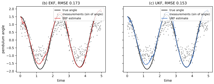
fig_S8_2. Reproduces Murphy (2023), Supplementary Figure 8.2. Download: PDF · SVG8.3.3 The extended Kalman smoother (EKS)
p. 379 Run the RTS recursion (8.65)–(8.69) with \(\mF_{t+1}\) the Jacobian of \(f\) at the filtered mean \(\bmu_{t|t}\) (code: eks, which equals the RTS smoother on linear models). The iterated EKS relinearises along the previous smoothed path and is Gauss–Newton for the MAP of the whole trajectory \(p(\vz_{1:T}\given\vy_{1:T})\), by the argument of Filling the gap 8.13 applied to the block-tridiagonal objective.
8.4 Inference based on the unscented transform
pp. 379–382, Algorithms 8.5–8.6 Instead of linearising the functions, approximate the joint distributions \(p(\vz_{t-1},\vz_t\given\vy_{1:t-1})\) and \(p(\vz_t,\vy_t\given\vy_{1:t-1})\) by Gaussians whose moments are computed by a deterministic point rule. With the unscented transform this is the unscented Kalman filter (UKF, or sigma-point filter). It needs no Jacobians and is usually more accurate; it costs \(2N_z+1\) evaluations of \(f\) and of \(h\) per step (the book says \(N_z\)) and has three tuning parameters.
8.4.1 The unscented transform
pp. 381–382, (8.148)–(8.151) With \(\lambda=\alpha^2(n+\kappa)-n\) and \(\mL\) a matrix square root of \(\bSig\) (\(\mL\mL^\T=\bSig\), e.g. Cholesky), the \(2n+1\) sigma points and weights are
\[ \mathcal X_0=\bmu,\quad \mathcal X_{\pm i}=\bmu\pm\sqrt{n+\lambda}\,\mL_{:,i},\qquad w^m_0=\tfrac{\lambda}{n+\lambda},\quad w^c_0=\tfrac{\lambda}{n+\lambda}+1-\alpha^2+\beta,\quad w^m_{\pm i}=w^c_{\pm i}=\tfrac1{2(n+\lambda)}. \]Push them through \(g\), \(\mathcal Y_i=g(\mathcal X_i)\) (8.148), and estimate \(\hat\vy=\sum_iw^m_i\mathcal Y_i\), \(\mS=\sum_iw^c_i(\mathcal Y_i-\hat\vy)(\mathcal Y_i-\hat\vy)^\T+\boldsymbol\Omega\), \(\mC=\sum_iw^c_i(\mathcal X_i-\bmu)(\mathcal Y_i-\hat\vy)^\T\) (8.149)–(8.151); in Algorithm 8.6 the undefined \(\bmu_U\) of lines 5–6 is \(\hat\vy\).
Result 8.3 (what the unscented transform gets exactly right) p. 382
For \(\vx\sim\N(\bmu,\bSig)\) and any \(\alpha,\beta,\kappa\) with \(n+\lambda>0\): (a) the mean \(\hat\vy\) is exact for every polynomial \(g\) of degree at most 3; (b) \(\hat\vy\), \(\mS\) and \(\mC\) are exact for affine \(g\); (c) for \(n=1\) and \(g(x)=x^2\) the variance is \(4\mu^2\sigma^2+(\kappa+\beta)\sigma^4\) (with \(\alpha=1\)), exact if and only if \(\kappa+\beta=2\).
Proof
Let \(\boldsymbol\delta_i=\mathcal X_i-\bmu\). The mean weights sum to \(\lambda/(n+\lambda)+2n/(2(n+\lambda))=1\); the set \(\{\boldsymbol\delta_i\}\) is symmetric, so every odd moment \(\sum_iw^m_i\boldsymbol\delta_i^{\otimes k}\), \(k\) odd, vanishes, as for the Gaussian; and \(\sum_iw^m_i\boldsymbol\delta_i\boldsymbol\delta_i^\T=2\cdot\tfrac{n+\lambda}{2(n+\lambda)}\sum_i\mL_{:,i}\mL_{:,i}^\T=\bSig\). (a) Expand \(g\) around \(\bmu\): constant, linear, quadratic and cubic terms in \(\boldsymbol\delta\). The rule reproduces the Gaussian's moments of orders 0, 1, 2, 3, so it integrates each term exactly. (b) For \(g(\vx)=\mA\vx+\mathbf b\), \(\mathcal Y_i-\hat\vy=\mA\boldsymbol\delta_i\) and \(\boldsymbol\delta_0=\mathbf0\), so the extra centre weight \(1-\alpha^2+\beta\) multiplies zero and \(\mS=\mA\bSig\mA^\T+\boldsymbol\Omega\), \(\mC=\bSig\mA^\T\). (c) is Problem 8.3. The fourth moment shows why: along an axis the rule gives \(\sum_iw_i\delta_i^4=(n+\lambda)\sigma^4\), the Gaussian \(3\sigma^4\), so the classical choice \(n+\kappa=3\) (with \(\alpha=1\)) matches it; \(\beta=2\) compensates through the centre weight instead. ∎
The code checks (a) on a cubic in 2d for three values of \(\kappa\), (b) for a random affine map, and (c) for four settings. The variance of a quadratic is a fourth-order quantity, so in general the UT covariance is exact only for affine maps, as the book says; higher-order rules with \(2n^2+1\) points fix quadratics.
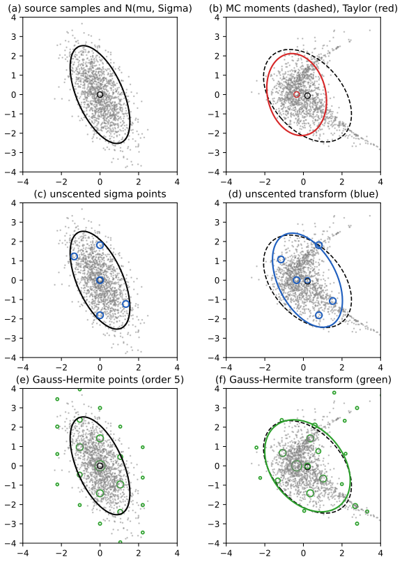
fig_8_5. Reproduces Murphy (2023), Figure 8.5. Download: PDF · SVG8.4.2 The unscented Kalman filter (UKF)
p. 382, (8.152)–(8.154) Replace LinGaussJoint in Algorithm 8.2 by UnscentedGaussJoint twice (once for \(f\) with noise \(\mQ_t\), once for \(h\) with \(\mR_t\)) and keep GaussCondition. On a linear model the UKF is exactly the Kalman filter, for any \(\alpha,\beta,\kappa\) (Result 8.3(b); confirmed to \(10^{-9}\)). Figure 8.4(c) used \(\alpha=1,\beta=0,\kappa=2\).
8.4.3 The unscented Kalman smoother (UKS)
p. 382 The RTS gain can be written with the predicted cross covariance, \(\mJ_t=\mathbf D_{t+1}\bSig_{t+1|t}^{-1}\) with \(\mathbf D_{t+1}=\cov[\vz_t,\vz_{t+1}\given\vy_{1:t}]\), and both factors can be computed with sigma points.
Filling the gap 8.15: why the RTS recursion survives the unscented approximation p. 382
The proof of Result 8.2 used only one thing: that \((\vz_t,\vz_{t+1})\) given \(\vy_{1:t}\) is jointly Gaussian with known moments.
Derivation
Replace that joint by its unscented Gaussian approximation: mean \((\bmu_{t|t},\bmu_{t+1|t})\), covariance blocks \(\bSig_{t|t}\), \(\mathbf D_{t+1}=\sum_iw^c_i(\mathcal X_i-\bmu_{t|t})(f(\mathcal X_i)-\bmu_{t+1|t})^\T\) and \(\bSig_{t+1|t}\). Conditioning on \(\vz_{t+1}\) gives (8.78)–(8.79) with \(\mJ_t=\mathbf D_{t+1}\bSig_{t+1|t}^{-1}\), and the rest of the proof is unchanged, giving (8.68)–(8.69). For linear \(f\), \(\mathbf D_{t+1}=\bSig_{t|t}\mF^\T\) and \(\mJ_t\) is (8.67); the code's uks equals the RTS smoother on a linear model to \(10^{-9}\). The same construction works for any point rule (cubature or Gauss–Hermite smoothers). ∎
The book notes one notable use: unscented smoothing of Bluetooth signal strength to estimate distances in a COVID-19 contact-tracing app.
8.5 Other variants of the Kalman filter
8.5.1 General Gaussian filtering
pp. 383–386, (8.155)–(8.177) The best Gaussian approximation of the joint \(p(\vz,\vy)=\N(\vz\given\bmu,\bSig)\,p(\vy\given\vz)\), in the sense of \(\min_q\KL(p\,\|\,q)\) (8.155), matches its moments: \(\hat\vy=\int h_\mu(\vz)\N(\vz\given\bmu,\bSig)\d\vz\), \(\mS=\boldsymbol\Omega+\int(h_\mu-\hat\vy)(h_\mu-\hat\vy)^\T\N\,\d\vz\), \(\mC=\int(\vz-\bmu)(h_\mu-\hat\vy)^\T\N\,\d\vz\) (8.156)–(8.159). Conditioning that Gaussian on \(\vy_t\) gives the general Gaussian filter (GGF) update (8.160)–(8.162), the Kalman update with \(\mK_t=\mC_t\mS_t^{-1}\).
Filling the gap 8.16: moment matching minimises the inclusive KL p. 383, (8.155)
The book refers to Section 5.1.4.2 (notes); the Gaussian case is two lines.
Derivation
For any \(p\) with mean \(\mathbf m\) and covariance \(\mathbf V\), \(\KL(p\,\|\,q)=-H(p)-\E_p\log q\), and for \(q=\N(\mathbf a,\mathbf B)\), \(-\E_p\log q=\tfrac12\log|2\pi\mathbf B|+\tfrac12\Tr(\mathbf B^{-1}\mathbf V)+\tfrac12(\mathbf m-\mathbf a)^\T\mathbf B^{-1}(\mathbf m-\mathbf a)\), which depends on \(p\) only through \(\mathbf m,\mathbf V\). It is minimised over \(\mathbf a\) at \(\mathbf a=\mathbf m\); then, with \(\mathbf P=\mathbf B^{-1}\), \(-\tfrac12\log|\mathbf P|+\tfrac12\Tr(\mathbf P\mathbf V)\) is convex in \(\mathbf P\) with gradient \(\tfrac12(\mathbf V-\mathbf P^{-1})\), zero at \(\mathbf B=\mathbf V\). So the optimal Gaussian has the moments of \(p\). Applied to the joint \(p(\vz,\vy)\) this gives (8.156)–(8.159). The opposite direction, \(\KL(q\,\|\,p)\), is mode seeking and does not reduce to moments. ∎
8.5.1.1 Statistical linear regression
pp. 383–384, (8.163)–(8.166) Equivalently, the GGF replaces the likelihood by the linear model \(q(\vy\given\vz)=\N(\mA\vz+\mathbf b,\boldsymbol\Omega)\) with
\[ \mA=\mC^\T\bSig^{-1},\qquad \mathbf b=\hat\vy-\mA\bmu,\qquad \boldsymbol\Omega=\mS-\mA\bSig\mA^\T, \tag{8.163} \]statistical linear regression (SLR): the best linear fit over the whole prior, rather than the tangent at \(\bmu\).
Filling the gap 8.17: SLR minimises the mean squared error and the expected KL p. 384, (8.164)–(8.166)
The book cites the literature for both claims.
Derivation
(8.165)–(8.166). Minimise \(\E\|\vy-\mA\vz-\mathbf b\|^2\) over \((\vz,\vy)\) from the joint. Setting derivatives to zero: \(\E[\vy-\mA\vz-\mathbf b]=\mathbf0\) and \(\E[(\vy-\mA\vz-\mathbf b)(\vz-\bmu)^\T]=\mathbf0\), i.e. \(\mathbf b=\hat\vy-\mA\bmu\) and \(\mC^\T-\mA\bSig=\mathbf0\); the objective is a convex quadratic, so this is the minimum. The residual \(\mathbf e=\vy-\mA\vz-\mathbf b\) has covariance \(\mS-\mC^\T\bSig^{-1}\mC=\mS-\mA\bSig\mA^\T\). (8.164). Let \(p(\vy\given\vz)=\N(h(\vz),\boldsymbol\Omega_0)\), so \(\mS\) includes \(\boldsymbol\Omega_0\). For Gaussians, \(\E_{\vz}\KL(p(\cdot\given\vz)\,\|\,q(\cdot\given\vz))=\tfrac12\E\big[\Tr(\boldsymbol\Omega^{-1}\boldsymbol\Omega_0)+\mathbf d^\T\boldsymbol\Omega^{-1}\mathbf d\big]-\tfrac{N_y}2+\tfrac12\log\tfrac{|\boldsymbol\Omega|}{|\boldsymbol\Omega_0|}\) with \(\mathbf d=h(\vz)-\mA\vz-\mathbf b\). For fixed \(\boldsymbol\Omega\) the minimiser over \((\mA,\mathbf b)\) of the weighted least-squares term satisfies the same normal equations as above (the weight \(\boldsymbol\Omega^{-1}\) multiplies both and cancels), so \((\mA,\mathbf b)\) are (8.163). Then the minimiser over \(\boldsymbol\Omega\) is \(\boldsymbol\Omega_0+\E\mathbf d\mathbf d^\T=\boldsymbol\Omega_0+\var[h]-\mA\bSig\mA^\T=\mS-\mA\bSig\mA^\T\). On 200,000 draws the least-squares fit and residual covariance match (8.163) to 0.01, and random perturbations of the SLR parameters always increase the expected KL. ∎
8.5.1.2 Approximating the moments
p. 384, (8.167)–(8.168) Everything reduces to Gaussian expectations \(g_e(f,\bmu,\bSig)=\int f\,\N\) and cross covariances \(g_c(f,g,\bmu,\bSig)\). The code has one function, moments_by_points, that computes \((\hat\vy,\mS,\mC)\) for any point rule; the filters differ only in the rule.
8.5.1.3 Approximation based on linearization
pp. 384–385, (8.169)–(8.176) Linearising gives \(g_c=\mF\bSig\mathbf G^\T\) and recovers the EKF. The tangents should read \(\hat f(\vz)=f(\bmu)+\mF(\vz-\bmu)\) and \(\hat g(\vz)=g(\bmu)+\mathbf G(\vz-\bmu)\), so \(g_e(\hat f)=f(\bmu)\); the book writes \(\bmu\) for \(f(\bmu)\) in (8.169)–(8.171) and (8.174). The covariance (8.176) is unaffected.
8.5.1.4 Approximation based on Gaussian quadrature (sigma points)
p. 385, (8.177) Point rules \(\int h\,\N\approx\sum_kw_kh(\vz_k)\): the unscented transform (the UKF), the spherical cubature rule (the CKF: \(2n\) points \(\bmu\pm\sqrt n\mL_{:,i}\), weights \(1/(2n)\)), and tensor-product Gauss–Hermite rules with \(p^n\) points (the GHKF or quadrature KF).
Filling the gap 8.18: Gauss–Hermite is exact to degree \(2p-1\), and the cubature rule is the UT with \(\kappa=0\) p. 385
The book states both with references; the second is misstated ("\(\kappa\) left free").
Derivation
Gauss–Hermite. Let \(x_1,\dots,x_p\) be the roots of the Hermite polynomial \(He_p\) (orthogonal for the weight \(\phi\), the standard normal density) and \(w_k\) the weights of the interpolating rule at these nodes, so the rule is exact for degree \(\le p-1\). For a polynomial \(f\) of degree \(\le2p-1\), divide: \(f=qHe_p+r\) with \(\deg q,\deg r\le p-1\). Then \(\int qHe_p\phi=0\) by orthogonality, and \(\sum_kw_kq(x_k)He_p(x_k)=0\) because the nodes are roots; the remainder \(r\) is integrated exactly. Hence exactness for degree \(2p-1\), and failure at \(x^{2p}\) (checked for \(p=2,3,5\)). In \(n\) dimensions the tensor rule in whitened coordinates \(\vx=\bmu+\mL\vu\) integrates every monomial \(u_1^{a_1}\cdots u_n^{a_n}\) with all \(a_i\le2p-1\) exactly, in particular every polynomial of total degree \(\le2p-1\): order 3 handles the variance of a quadratic (Filling the gap 8.11). Cubature. With \(\alpha=1\), \(\kappa=0\): \(\lambda=0\), the points are \(\bmu\pm\sqrt n\mL_{:,i}\), \(w^m_0=0\), \(w_{\pm i}=1/(2n)\), and \(w^c_0=\beta\), so \(\beta=0\) is also needed. That is the cubature rule exactly. With \(\kappa\ne0\) the points move to \(\pm\sqrt{n+\kappa}\) and the centre gets weight \(\kappa/(n+\kappa)\), a different rule (the code finds covariances differing by more than \(10^{-3}\) for \(\kappa=1\)). So the CKF is the UKF with \(\alpha=1,\beta=0,\kappa=0\). ∎
8.5.1.5 Approximation based on Monte Carlo integration
p. 385 Monte Carlo moments give a randomised GGF; this still approximates the joint of state and observation, unlike a particle filter, which approximates the posterior itself.
8.5.2 Conditional moment Gaussian filtering
pp. 386–387, (8.178)–(8.188) For non-Gaussian likelihoods it is enough to know the conditional mean \(h_\mu(\vz)=\E[\vy\given\vz]\) and covariance \(h_\Sigma(\vz)=\cov[\vy\given\vz]\) (8.178)–(8.179). Then
\[ \hat\vy=g_e(h_\mu),\qquad \mC=g_c(\vz,h_\mu),\qquad \mS=g_e(h_\Sigma)+g_c(h_\mu,h_\mu), \tag{8.180–8.185} \]and the GGF update applies: conditional moments Gaussian filtering (CMGF). Examples: Poisson, \(h_\mu=h_\Sigma=c\,e^{z}\) (8.186); categorical with logits \(h(\vz)\), \(h_\mu=\mathbf p=\mathrm{softmax}(h(\vz))\), \(h_\Sigma=\diag(\mathbf p)-\mathbf p\mathbf p^\T\) (8.188), dropping one class to keep \(\mS\) invertible.
Filling the gap 8.19: the conditional-moment formulas, with closed forms p. 386
(8.180)–(8.185) are the laws of total expectation and covariance; two examples have closed forms worth knowing.
Derivation
\(\E\vy=\E\E[\vy\given\vz]\); \(\cov[\vz,\vy]=\E[(\vz-\bmu)(\vy-\hat\vy)^\T]=\E[(\vz-\bmu)(h_\mu(\vz)-\hat\vy)^\T]\) by conditioning on \(\vz\) inside; \(\var\vy=\E\var[\vy\given\vz]+\var\E[\vy\given\vz]\). Poisson with \(z\sim\N(\mu,\sigma^2)\): the lognormal moments give \(\hat y=c\,e^{\mu+\sigma^2/2}\), \(S=\hat y+\hat y^2(e^{\sigma^2}-1)\) (overdispersed relative to the Poisson), and by Stein's lemma \(\cov[z,g(z)]=\sigma^2\E g'(z)\), \(C=\sigma^2\hat y\). Categorical: \(\E[\diag(\mathbf p)-\mathbf p\mathbf p^\T]+\var[\mathbf p]=\diag(\E\mathbf p)-\E\mathbf p\,\E\mathbf p^\T\), because \(\E[\mathbf p\mathbf p^\T]\) cancels: the marginal covariance is that of a single categorical with probabilities \(\E\mathbf p\), as it must be for a one-hot vector. Both confirmed by Gauss–Hermite quadrature to \(10^{-9}\). ∎
Exponential-family EKF (supplement 8.3)
Supp. pp. 91–98, (S8.61)–(S8.113), Figures S8.3–S8.4 The exponential-family EKF (EEKF; Ollivier, 2018) keeps the Gaussian dynamics and takes the observation in an exponential family with mean parameter \(\hat\vy_t=h(\vz_t,\vu_t)\). After the usual prediction it uses the sufficient statistic and its covariance in place of the Gaussian innovation and noise,
\[ \mathbf e_t=\mathcal T(\vy_t)-\hat\vy_t,\quad \mR_t=\cov[\mathcal T(\vy)\given\hat\vy_t],\quad \mK_t=\bSig_{t|t-1}\mH_t^\T(\mH_t\bSig_{t|t-1}\mH_t^\T+\mR_t)^{-1},\quad \bSig_t=(\mI-\mK_t\mH_t)\bSig_{t|t-1},\quad \bmu_t=\bmu_{t|t-1}+\mK_t\mathbf e_t. \tag{S8.68–S8.73} \]For a Bernoulli label with \(\hat y=\sigma(\vz^\T\vx)\): \(\mathcal T(y)=y\), \(R=\hat y(1-\hat y)\), \(\mH=\hat y(1-\hat y)\vx^\T\). Figures S8.3 and S8.4 apply it, with static weights, to the logistic-regression data used for ADF in Section 8.6.3.
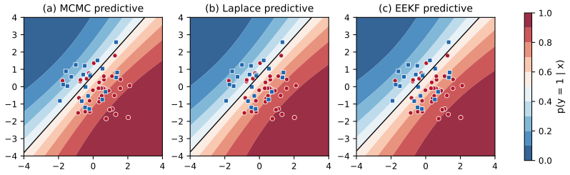
fig_S8_3. Reproduces Murphy (2023), Supplementary Figure 8.3 (simulated stand-in data). Download: PDF · SVG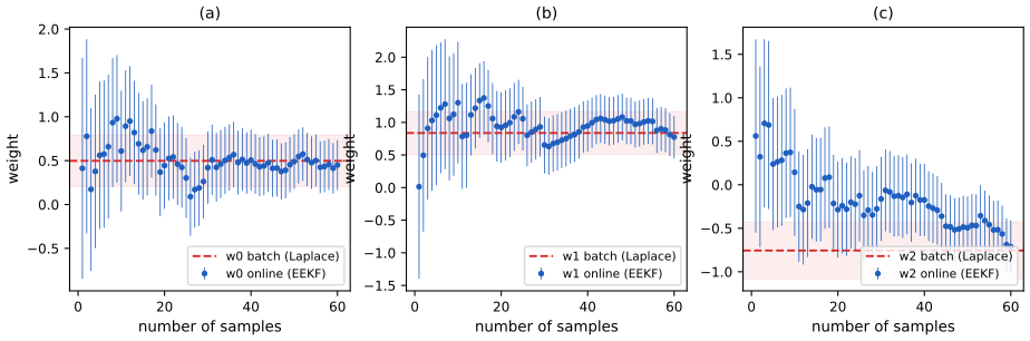
fig_S8_4. Reproduces Murphy (2023), Supplementary Figure 8.4. Download: PDF · SVGThe supplement proves (Theorem 1) that with static dynamics the EEKF is online natural-gradient descent (Section 6.4) with learning rate \(\eta_t=\gamma_t=1/(t+1)\) and Fisher matrix \(\mathbf J_t=\bSig_t^{-1}/(t+1)\):
\[ \mathbf J_t=(1-\gamma_t)\mathbf J_{t-1}+\gamma_t\E_{p(\vy|\hat\vy_t)}[\nabla\mathcal L_t\nabla\mathcal L_t^\T],\qquad \boldsymbol\theta_t=\boldsymbol\theta_{t-1}-\eta_t\mathbf J_t^{-1}\nabla\mathcal L_t,\qquad \mathcal L_t=-\log p(\vy_t\given\hat\vy_t). \tag{S8.80–S8.81} \]Filling the gap 8.20: the EKF as natural-gradient descent, with two corrections Supp. pp. 94–98, Lemmas 1–4, Theorems 1–2
The supplement's chain of lemmas is right in substance, but Theorem 2's proof changes sign halfway and Lemma 3 has \(\mR_t\) where \(\mR_t^{-1}\) belongs. Here is the chain, corrected.
Derivation
Lemma 1: \(\mathcal T(\vy)-\hat\vy=\mR\nabla_{\hat\vy}\log p(\vy\given\hat\vy)\). With natural parameter \(\beta\), \(\log p=\beta^\T\mathcal T(\vy)-A(\beta)\), so \(\nabla_\beta\log p=\mathcal T(\vy)-\nabla A=\mathcal T(\vy)-\hat\vy\); and \(\partial\hat\vy/\partial\beta=\nabla^2A=\cov\mathcal T=\mR\) (symmetric), so the chain rule gives \(\nabla_\beta\log p=\mR\nabla_{\hat\vy}\log p\). Lemma 2: \(\mK_t\mR_t=\bSig_t\mH_t^\T\): \(\mK\mR=\mK(\mR+\mH\bSig\mH^\T)-\mK\mH\bSig\mH^\T=(\mI-\mK\mH)\bSig\mH^\T\). Theorem 2 (corrected sign): with \(\nabla_{\hat\vy}\mathcal L=-\nabla_{\hat\vy}\log p\) and \(\nabla_{\bmu}\mathcal L=\mH^\T\nabla_{\hat\vy}\mathcal L\),
\[ \bmu_t=\bmu_{t|t-1}+\mK_t\mathbf e_t=\bmu_{t|t-1}-\mK_t\mR_t\nabla_{\hat\vy}\mathcal L_t=\bmu_{t|t-1}-\bSig_t\nabla_{\bmu}\mathcal L_t, \]which is (S8.95); the supplement's (S8.98)–(S8.100) carry \(+\). Lemma 3: by Woodbury, \(\bSig_t^{-1}=\bSig_{t|t-1}^{-1}+\mH_t^\T\mR_t^{-1}\mH_t\) (the printed (S8.102) has \(\mR_t\)). Lemma 4: the Fisher information for the mean parameter is \(\E[\nabla_{\hat\vy}\log p\nabla_{\hat\vy}\log p^\T]=\mR^{-1}\E[(\mathcal T-\hat\vy)(\mathcal T-\hat\vy)^\T]\mR^{-1}=\mR^{-1}\), so \(\E[\nabla_{\bmu}\mathcal L\nabla_{\bmu}\mathcal L^\T]=\mH^\T\mR^{-1}\mH\). Theorem 1: with static dynamics, \(\bSig_t^{-1}=\bSig_{t-1}^{-1}+\E[\mathbf g\mathbf g^\T]\); dividing by \(t+1\) and setting \(\mathbf J_t=\bSig_t^{-1}/(t+1)\) gives \(\mathbf J_t=\tfrac t{t+1}\mathbf J_{t-1}+\tfrac1{t+1}\E[\mathbf g\mathbf g^\T]\), and Theorem 2 becomes \(\bmu_t=\bmu_{t-1}-\tfrac1{t+1}\mathbf J_t^{-1}\nabla\mathcal L_t\), started at \(\mathbf J_0=\bSig_0^{-1}\). The code runs both recursions on the 60 logistic examples and they agree to \(10^{-9}\) at every step. Fading memory: inflating \(\bSig_{t-1}\) by \(1/(1-\lambda_t)\) with \(1-\lambda_t=\eta_{t-1}/\eta_t-\eta_{t-1}\) (S8.83) emulates other learning rates: \(\eta_t\equiv\eta_0\) gives \(\lambda_t=\eta_0\), \(\eta_t=1/(t+c)\) gives \(\lambda_t=0\). ∎
8.5.3 Iterated filters and smoothers
pp. 387–388, Algorithm 8.7 The iterated posterior linearisation filter (IPLF) recomputes the SLR moments over the current posterior \(\N(\bmu_{t|t},\bSig_{t|t})\) and conditions the prior again, \(J\) times; the smoother analogue is the IPLS. These are the SLR counterparts of the iterated EKF and EKS, and like them can diverge without damping.
Algorithm 8.7 (iterated conditional moments Gaussian filter)
- For each \(t\): predict \((\bmu_{t|t-1},\bSig_{t|t-1})\) with the moments of \(f\) under \(\N(\bmu_{t-1|t-1},\bSig_{t-1|t-1})\) plus \(\mQ\).
- Set \((\bmu_{t|t},\bSig_{t|t})=(\bmu_{t|t-1},\bSig_{t|t-1})\); repeat \(J\) times: compute the SLR \((\mA,\mathbf b,\boldsymbol\Omega)\) of \((h_\mu,h_\Sigma)\) under \(\N(\bmu_{t|t},\bSig_{t|t})\), then do the Kalman update of the prior \((\bmu_{t|t-1},\bSig_{t|t-1})\) with the linear model \(\N(\mA\vz+\mathbf b,\boldsymbol\Omega)\).
This is the reading under which iterating is sound (compare Filling the gap 8.13): the moments are recomputed under the posterior, but they are turned into a linear model by SLR before the prior is conditioned. Feeding the posterior moments \((\hat\vy,\mS,\mC)\) directly into GaussCondition with the prior, as lines 8–9 of the printed algorithm do, mixes two distributions, the same issue as in Algorithm 8.4.
8.5.4 Ensemble Kalman filter
pp. 388–390, (8.189)–(8.194) The ensemble Kalman filter (EnKF), from data assimilation in geoscience, represents the belief by \(N_s\) samples (columns of \(\mathbf Z_{t|t}\)). Each member is propagated through the dynamics with its own noise, perturbed predicted observations are drawn, and every member is moved by a Kalman-type update with a gain estimated from the ensemble,
\[ \mathbf Z_{t|t}=\mathbf Z_{t|t-1}+\tilde\mK_t(\vy_t\mathbf 1^\T-\mathbf Y_{t|t-1}),\qquad \tilde\mK_t=\tilde\mC_t\tilde\mS_t^{-1}, \tag{8.191–8.194} \]with \(\tilde\mC_t,\tilde\mS_t\) the sample cross covariance and covariance of the anomalies. For additive noise one can use \(\tilde\mS_t=\tfrac1{N_s-1}\tilde{\mathbf O}\tilde{\mathbf O}^\T+\mR_t\) with \(\tilde{\mathbf O}=\mH\tilde{\mathbf Z}\) to reduce variance. The cost is linear in \(N_z\) for sparse dynamics, which is what makes it usable for states with millions of components; small ensembles are overconfident, hence covariance inflation.
Filling the gap 8.21: why the observations must be perturbed, and the large-ensemble limit pp. 388–389
The book says the EnKF does not converge to the posterior except in the linear-Gaussian case. Here is why it does in that case, and why the perturbation is needed.
Derivation
Linear model, forecast members \(\vz^{(s)}\) i.i.d. \(\N(\bmu,\bSig)\), exact gain \(\mK\) (the limit of \(\tilde\mK_t\) as \(N_s\to\infty\), by the law of large numbers). The analysis member \(\vz^{(s)}+\mK(\vy-\mH\vz^{(s)}-\mathbf r^{(s)})\), with \(\mathbf r^{(s)}\sim\N(\mathbf0,\mR)\) independent, has mean \(\bmu+\mK(\vy-\mH\bmu)\) and covariance \((\mI-\mK\mH)\bSig(\mI-\mK\mH)^\T+\mK\mR\mK^\T=(\mI-\mK\mH)\bSig\), the Joseph form of Filling the gap 8.4, which is the posterior covariance. Without the perturbation the covariance would be \((\mI-\mK\mH)\bSig(\mI-\mK\mH)^\T\), too small by \(\mK\mR\mK^\T\). Since the members are affine images of Gaussians, they are exactly posterior samples in the limit. In a nonlinear model the update is still a linear shift of each member, so the ensemble cannot represent a skewed or multimodal posterior. With 20,000 members, both gains give means within 0.02 of the Kalman filter on the tracking data of Figure 8.2. ∎
8.5.5 Robust Kalman filters
p. 390 Outliers and sudden jumps call for heavy-tailed noise (Laplace or Student). Variational Bayes can keep a Gaussian state posterior while learning a noise scale with an inverse-Wishart distribution. Section 8.7.1 shows what exact inference does with Student noise: a bimodal posterior.
8.5.6 Dual EKF
p. 390 To learn parameters online, augment the state with \(\boldsymbol\theta_t\), given artificial dynamics \(\N(\boldsymbol\theta_{t-1},\epsilon\mI)\), and run two coupled EKFs, one for the states and one for the parameters. The drift slider of the logistic demonstration is this artificial dynamics.
8.5.7 Normalizing flow KFs
pp. 390–391 If \(\vy_t=f_t(\mathbf h_t)\) with \(\mathbf h_t=\mH_t\vz_t+\mathbf r_t\) and \(f_t\) invertible, the Jacobian factor of \(p(\vy_t\given\vz_t)\) does not depend on \(\vz_t\) and cancels in Bayes' rule, so the exact posterior is the Kalman filter applied to \(f_t^{-1}(\vy_t)\) (the book's proof is complete; the code confirms it by quadrature for \(f=\exp\)).
8.6 Assumed density filtering
pp. 391–392, (8.195)–(8.198), Figure 8.6 Assumed density filtering (ADF) keeps the belief in a tractable family \(\mathcal Q\): predict (8.195), update exactly with the new likelihood (8.196)–(8.197), then project back onto \(\mathcal Q\),
\[ q_t=\argmin_{q\in\mathcal Q}\KL\big(p_t(\vz_t\given\vy_{1:t})\,\|\,q(\vz_t)\big), \tag{8.198} \]a moment projection: for Gaussians, match the mean and covariance (Filling the gap 8.16).
8.6.1 Connection with Gaussian filtering
pp. 392–393, (8.199), Figure 8.7 The GGF moment-matches the joint \(p(\vz_t,\vy_t\given\vy_{1:t-1})\) and then conditions; ADF moment-matches the posterior \(p(\vz_t\given\vy_{1:t})\). The two coincide when the likelihood is linear-Gaussian. ADF is the more accurate of the two (it matches the moments of the exact one-step posterior), but its moment integrals involve the normaliser \(Z_t\) and are usually harder.
8.6.2 ADF for SLDS (Gaussian sum filter)
pp. 393–394, (8.200)–(8.208), Figure 8.8 For a switching linear dynamical system with \(K\) modes, keep one Gaussian per mode, \(b^i_{t-1}=\pi^i_{t-1}\N(\bmu^i,\bSig^i)\). GPB2 runs the \(K^2\) Kalman filters (from mode \(i\) through the dynamics of mode \(j\)), then for each \(j\) collapses the \(K\) Gaussians into one by moment matching,
\[ \bmu=\sum_k\pi_k\bmu_k,\qquad \bSig=\sum_k\pi_k\big(\bSig_k+(\bmu_k-\bmu)(\bmu_k-\bmu)^\T\big) \tag{8.203–8.204} \]("weak marginalisation"). IMM collapses before filtering instead, needing only \(K\) filters.
Filling the gap 8.22: the collapse, and the right weights in GPB2 pp. 393–394, (8.201)–(8.208)
Three points in the printed equations need fixing: the direction of the KL in the collapse, the posterior weights of the \(K^2\) components, and the normalisation in (8.206).
Derivation
Collapse. A mixture has mean \(\sum_k\pi_k\bmu_k\) and, by the law of total covariance, \(\sum_k\pi_k\bSig_k+\sum_k\pi_k(\bmu_k-\bmu)(\bmu_k-\bmu)^\T\). By Filling the gap 8.16 the Gaussian with these moments minimises \(\KL(p\,\|\,q)\); the text above (8.203) writes \(\KL(q\,\|\,p)\), whose minimiser is not given by moments (and usually locks onto one component). Weights. After filtering component \((i,j)\) with \(\vy_t\), Bayes' rule gives \(p(m_{t-1}=i,m_t=j\given\vy_{1:t})\propto\pi^i_{t-1}A_{ij}\,\N(\vy_t\given\hat\vy^{ij}_t,\mS^{ij}_t)\): the prior weight times the predictive likelihood of that filter. (8.201) gives \(\pi^{ij}_{t|t}=\pi^i_{t-1}A_{ij}\), the prior weight; in a two-mode example the posterior weights are (0.872, 0.067, 0.010, 0.052) against the prior (0.63, 0.07, 0.06, 0.24). Normalisation. To merge over \(i\) for fixed \(j\) the weights must be \(\pi^{ij}/\sum_{i'}\pi^{i'j}\) (a distribution over \(i\)); (8.206) normalises over \(j'\), which gives weights over \(i\) that do not sum to one (1.087 in the example). Then \(\pi^j=\sum_i\pi^{ij}\), \(\bmu^j=\sum_i\pi_{i|j}\bmu^{ij}\), \(\bSig^j=\sum_i\pi_{i|j}(\bSig^{ij}+(\bmu^{ij}-\bmu^j)(\bmu^{ij}-\bmu^j)^\T)\). ∎
8.6.3 ADF for online logistic regression
pp. 394–397, (8.209)–(8.223), Figures 8.9–8.12 Model: \(p(y_t\given\vx_t,\vw_t)=\Ber(y_t\given\sigma(\vx_t^\T\vw_t))\), \(p(\vw_t\given\vw_{t-1})=\N(\vw_{t-1},\mQ)\) with \(\mQ=\epsilon\mI\) (or 0). The belief is a diagonal Gaussian \(\prod_j\N(w_j\given\mu_j,\tau_j)\). The logit \(\eta_t=\vx_t^\T\vw_t\) has prior \(\N(m_{t|t-1},v_{t|t-1})\), \(m=\sum_jx_j\mu_j\), \(v=\sum_jx_j^2\tau_j\) (8.212)–(8.214); its tilted moments \(m_t,v_t\) under \(\Ber(y_t\given\sigma(\eta))\N(\eta\given m,v)\) (the book writes \(\Ber(y_t\given\eta_t)\)) are one-dimensional integrals (8.215)–(8.218), computed here by a 801-point rule on \(\pm8\) standard deviations. Then, with \(\delta m=m_t-m\), \(\delta v=v_t-v\),
\[ \mu_{i,t|t}=\mu_{i,t|t-1}+a_i\,\delta m,\qquad \tau_{i,t|t}=\tau_{i,t|t-1}+a_i^2\,\delta v,\qquad a_i=\frac{x_{t,i}\,\tau_{i,t|t-1}}{\sum_jx_{t,j}^2\,\tau_{j,t|t-1}}. \tag{8.221–8.223} \]The book prints the denominator of \(a_i\) as \(\sum_j(x^j_t)^2+\tau^j_{t|t-1}\); it is the product, i.e. \(v_{t|t-1}\).
Filling the gap 8.23: the ADF update is exact moment matching of the tilted posterior p. 396, (8.219)–(8.223)
The book derives the update from "soft evidence" on \(\eta\) through \(p(\eta\given\vw)=\N(\eta\given\vw^\T\vx_t,0)\) (printed with \(\vw^\T\eta_t\)). Here is a derivation that also shows the result is the exact KL projection onto diagonal Gaussians.
Derivation
Let the prior be \(\vw\sim\N(\bmu,\bSig)\), \(\bSig=\diag(\boldsymbol\tau)\), and \(\eta=\vx^\T\vw\), so \((\vw,\eta)\) is jointly Gaussian with \(\cov[\vw,\eta]=\bSig\vx\), \(\var\eta=v\). The exact posterior is \(\hat p(\vw)\propto\ell(\vx^\T\vw)\N(\vw\given\bmu,\bSig)\), with \(\ell\) the likelihood. The joint \(\hat p(\vw,\eta)\propto\ell(\eta)\,\N(\eta\given m,v)\,\N(\vw\given\eta)\), where \(\N(\vw\given\eta)\) is the Gaussian conditional; so given \(\eta\) the tilting changes nothing: \(\hat p(\vw\given\eta)=\N(\vw\given\bmu+\mathbf a(\eta-m),\ \bSig-\mathbf a\mathbf a^\T v)\), \(\mathbf a=\bSig\vx/v\) (Filling the gap 8.3). Averaging over \(\hat p(\eta)\), which has mean \(m_t\) and variance \(v_t\): \(\E_{\hat p}\vw=\bmu+\mathbf a\,\delta m\) and \(\cov_{\hat p}\vw=\bSig-\mathbf a\mathbf a^\T v+\mathbf a\mathbf a^\T v_t=\bSig+\mathbf a\mathbf a^\T\delta v\) (law of total covariance). The diagonal of this is (8.221)–(8.222) with \(a_i=x_i\tau_i/v\). Projection. For a product \(q=\prod_iq_i\), \(\KL(\hat p\,\|\,q)=\KL(\hat p\,\|\,\prod_i\hat p_i)+\sum_i\KL(\hat p_i\,\|\,q_i)\), minimised by matching each marginal's mean and variance, which is exactly these diagonal entries. So ADF here is exact moment projection, dropping only the off-diagonal \(\mathbf a\mathbf a^\T\delta v\). Importance sampling with 400,000 draws confirms the moments; the printed \(a_i\) gives visibly different updates. ∎
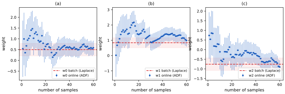
fig_8_10. Reproduces Murphy (2023), Figure 8.10 (simulated stand-in data). Download: PDF · SVG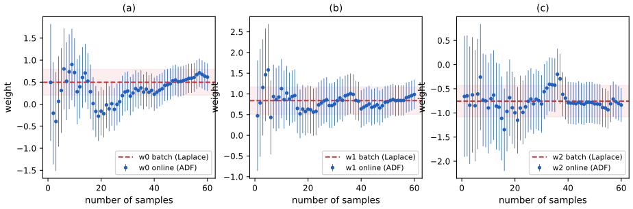
fig_8_11. Reproduces Murphy (2023), Figure 8.11. Download: PDF · SVG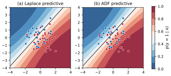
fig_8_12. Reproduces Murphy (2023), Figure 8.12. Download: PDF · SVGADF costs \(O(D)\) per example, like SGD, but has no step size: the variances set the step for each weight. It is close in spirit to the iterated posterior linearisation filter, but approximates the posterior rather than the joint (Section 8.6.1).
8.6.4 ADF for online DNNs
p. 398 The same predict-update-project cycle, with moments propagated through the layers, trains Bayesian neural networks online (book Section 17.5.3).
8.7 Other inference methods for SSMs
8.7.1 Grid-based approximations
pp. 398–399, (8.224)–(8.225), Figures 8.13–8.14 Discretise the state on a grid and run the HMM filter and smoother. With \(B\) bins per dimension there are \(K=B^{N_z}\) states and \(O(K^2)\) work per step, so this is only for one or two dimensions, where it handles any likelihood. The example has heavy-tailed Student noise in both equations,
\[ z_t=z_{t-1}+\mathcal T_2(0,1),\qquad y_t=z_t+\mathcal T_2(0,1). \tag{8.224–8.225} \]Filling the gap 8.24: the grid filter is an HMM filter, and it is exact in the fine-grid limit p. 398
The book describes the method in words.
Derivation
On grid points \(g_1,\dots,g_K\), replace the state density by a probability vector \(\mathbf p\) and the transition by the stochastic matrix \(A_{ij}\propto p(z_t=g_j\given z_{t-1}=g_i)\) (rows normalised). Then (8.4) becomes \(\mathbf p_{t|t-1}=A^\T\mathbf p_{t-1|t-1}\), (8.5) becomes \(p_{t|t}(j)\propto p_{t|t-1}(j)\,p(y_t\given g_j)\) with normaliser \(\approx p(y_t\given y_{1:t-1})\), and (8.13) becomes \(p_{t|T}(i)=p_{t|t}(i)\sum_jA_{ij}p_{t+1|T}(j)/p_{t+1|t}(j)\): the forward–backward algorithm of the HMM (companion course, Section 13.2.2). Each sum is a Riemann sum for the corresponding integral, so for continuous, bounded densities and a grid that covers the mass, the approximation converges as the spacing shrinks. On a linear-Gaussian AR(1) model with 2,401 points the grid filter matches the Kalman means and log likelihood to \(10^{-6}\). ∎
With one measurement far from the predicted state (an outlier, placed at \(t=20\) in our simulation, \(y_{20}=11.1\) while \(z_{20}=-0.86\)), the Student likelihood does not let it drag the estimate: the filtered marginal at \(t=20\) has two modes, near 2.0 (what the dynamics predict) and near 10.9 (the reading), with 56% of the mass near the outlier; the filtered mean 6.49 lies between them, where there is little probability. The smoother, which also sees the next readings, puts the mass back near the truth (mean 0.96, one mode). A Kalman filter with Gaussian noise would have to move part way towards the outlier and could never represent the two explanations.
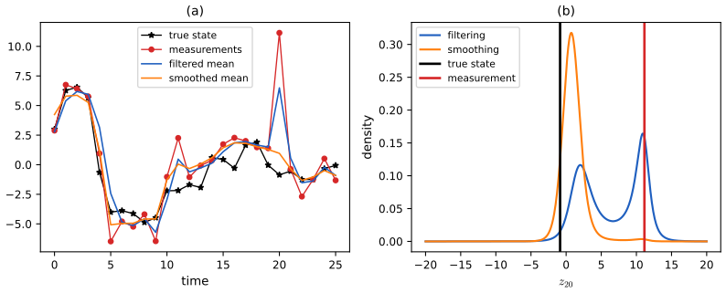
fig_8_13. Reproduces Murphy (2023), Figure 8.13 (simulated stand-in). Download: PDF · SVG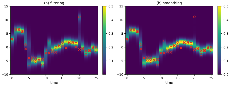
fig_8_14. Reproduces Murphy (2023), Figure 8.14. Download: PDF · SVG8.7.2 Expectation propagation
p. 398 EP (book Section 10.7) is iterated ADF: each local likelihood is combined with approximate messages from both past and future, the result is projected back onto the Gaussians, and the sweep is repeated.
8.7.3 Variational inference
p. 399 EP locally minimises the inclusive \(\KL(p\,\|\,q)\); variational inference globally minimises the exclusive \(\KL(q(\vz_{1:T})\,\|\,p(\vz_{1:T}\given\vy_{1:T}))\), which gives a lower bound that can be optimised stochastically and is guaranteed to converge.
8.7.4 MCMC
pp. 399–400 For HMMs and LG-SSMs, blocked Gibbs sampling alternates FFBS draws of the whole path (Filling the gap 8.9) with draws of the parameters; otherwise gradient-based HMC on the states, which scales poorly with \(T\).
8.7.5 Particle filtering
p. 400 Particle filters (book Section 13.2) replace the Gaussian by weighted samples, combining sequential importance sampling with resampling; EKF or UKF steps make good proposals. The basics are in Section 13.3.4 of the companion course.
Practice problems
Chapter 8 of the book has no end-of-chapter exercises. Here are three short problems with worked solutions.
Problem 8.1. For the local-level model \(z_t=z_{t-1}+q_t\), \(y_t=z_t+r_t\) with \(\var q_t=q\), \(\var r_t=r\), find the steady-state predicted variance \(P\) and gain \(k\), and show that the filter mean is an exponentially weighted moving average. Evaluate for \(q=r=1\).
Solution
The filtered variance is \(\Sigma=Pr/(P+r)\) and the next predicted variance is \(\Sigma+q\). At a fixed point \(P=Pr/(P+r)+q\), i.e. \(P^2-qP-qr=0\), whose positive root is \(P=\tfrac12(q+\sqrt{q^2+4qr})\); the gain is \(k=P/(P+r)\). The mean update \(\mu_t=\mu_{t-1}+k(y_t-\mu_{t-1})=(1-k)\mu_{t-1}+ky_t\) is exponential smoothing with weights \(k(1-k)^j\) on \(y_{t-j}\). (The variance recursion is a contraction for \(q,r>0\), so it converges from any start.) For \(q=r=1\): \(P=(1+\sqrt5)/2=1.618\) and \(k=0.618\), the golden ratio and its inverse; the code's filter reaches these values to \(10^{-12}\).
Problem 8.2. For a static state (\(\mF=\mI\), \(\mQ=\mathbf0\), as in RLS), show that every smoothed marginal equals the final filtered one: \(\bmu_{t|T}=\bmu_{T|T}\) and \(\bSig_{t|T}=\bSig_{T|T}\). Why is this obvious?
Solution
Here \(\bSig_{t+1|t}=\bSig_{t|t}\) and \(\bmu_{t+1|t}=\bmu_{t|t}\), so \(\mJ_t=\mI\). Then (8.68) gives \(\bmu_{t|T}=\bmu_{t|t}+\bmu_{t+1|T}-\bmu_{t|t}=\bmu_{t+1|T}\) and (8.69) gives \(\bSig_{t|T}=\bSig_{t+1|T}\); by backward induction all equal the values at \(T\). It is obvious because \(\vz_1=\dots=\vz_T\) is one unknown, so its posterior given all the data is the same whichever time index we attach to it. (Confirmed numerically to \(10^{-10}\).)
Problem 8.3. Let \(x\sim\N(\mu,\sigma^2)\) and \(y=x^2\). Compute the unscented mean and variance of \(y\) with \(n=1\), \(\alpha=1\) and general \(\beta,\kappa\), and compare with the exact values \(\mu^2+\sigma^2\) and \(4\mu^2\sigma^2+2\sigma^4\).
Solution
\(\lambda=\kappa\); points \(\mu\) and \(\mu\pm\sqrt{1+\kappa}\,\sigma\); weights \(w^m_0=\kappa/(1+\kappa)\), \(w^c_0=\kappa/(1+\kappa)+\beta\), \(w_\pm=1/(2(1+\kappa))\). Mean: \(\tfrac\kappa{1+\kappa}\mu^2+\tfrac1{1+\kappa}(\mu^2+(1+\kappa)\sigma^2)=\mu^2+\sigma^2\), exact. Deviations from the mean: \(-\sigma^2\) at the centre and \(\pm2\mu\sqrt{1+\kappa}\,\sigma+\kappa\sigma^2\) at the side points. Variance: \((\tfrac\kappa{1+\kappa}+\beta)\sigma^4+\tfrac1{1+\kappa}(4\mu^2(1+\kappa)\sigma^2+\kappa^2\sigma^4)=4\mu^2\sigma^2+(\kappa+\beta)\sigma^4\). It is exact if and only if \(\kappa+\beta=2\): \(\kappa=2,\beta=0\) (the rule \(n+\kappa=3\)) or \(\kappa=0,\beta=2\) (the usual "\(\beta=2\) is optimal for Gaussians"). With the cubature setting \(\kappa=\beta=0\) the variance is \(4\mu^2\sigma^2\), the same as linearisation. Checked for four settings.
Demonstrations for this chapter
Each demonstration runs in the browser, with seeded random numbers, and links back to these notes. Their numbers (errors, log likelihoods, moments, KL divergences, posterior means) are those of the Python code.
| Demonstration | What you can see | Sections |
|---|---|---|
| Kalman filtering, smoothing and fixed lag | 2d tracking with constant-velocity or spiral dynamics; filter, fixed-lag and RTS paths with 95% ellipses and errors over time. Presets: 1 Figure 8.2; 2 poor sensor; 3 manoeuvring target, lag 5; 4 spiral (Figure S8.1); 5 nearly deterministic motion. | 8.1.1, 8.2.2, 8.2.3, S8.1.1 |
| Gaussian through a nonlinear map | Taylor, unscented and Gauss–Hermite approximations against the exact moments, with \(\alpha,\beta,\kappa\), the order, the spread and the nonlinearity. Presets: 1 Figure 8.5; 2 small spread; 3 large spread; 4 cubature; 5 strong nonlinearity. | 8.3.1, 8.4.1, 8.5.1 |
| Online logistic regression by filtering | ADF and the EEKF against the Laplace approximation, weight traces and predictive maps. Presets: 1 Figure 8.10; 2 Figure 8.11; 3 EEKF (Figure S8.4); 4 drift; 5 tight prior. | 8.6.3, S8.3 |
The Python code that produces every figure of this page is code/ch08_gaussian_filtering_smoothing.py (see the code index).
Errors and slips found in the book
Everything below was confirmed by recomputation. Items marked (minor) are notational.
- (8.45): the observation block is \(\mH_t\bSig_{t|t-1}\mH_t^\T+\mR_t\), not \(\mH_t\bSig_{t|t-1}^{-1}\mH_t^\T+\mR_t\) (Section 8.2.2.4).
- (8.111)–(8.115): the information smoother must use \(\mF_{t+1},\mQ_{t+1}\) for the step \(t\to t+1\) (as (8.120) does), and (8.115), like (8.120), omits the offset terms present when \(\mathbf B\vu+\mathbf b\ne\mathbf0\); (8.113) also has a bare \(\mF\) (Filling the gap 8.10).
- Algorithm 8.4: relinearising with \((\bmu_{t|t},\bSig_{t|t})\) and \(\hat\vy=h(\bmu_{t|t})\), then conditioning the prior, does not converge to the MAP (8.146); each iteration must use the prior covariance and the predicted observation \(h(\vz_j)+\mH_j(\bmu_{t|t-1}-\vz_j)\) (Filling the gap 8.13). Lines 8–9 of Algorithm 8.7 have the same issue unless read as an SLR step.
- (8.140): \(\mF_t\) is the Jacobian of \(f\) at \(\bmu_{t-1|t-1}\), not at \(\bmu_{t|t-1}\).
- (8.201), (8.206): the GPB2 component weights need the predictive likelihood of \(\vy_t\), and collapsing over \(i\) must normalise over \(i\), not \(j'\); above (8.203), moment matching minimises \(\KL(p\,\|\,q)\), not \(\KL(q\,\|\,p)\) (Filling the gap 8.22).
- (8.223): \(a_i=x_i\tau_i/\sum_jx_j^2\tau_j\) (printed with a sum \(x_j^2+\tau_j\)); also \(p(y_t\given\eta_t)=\Ber(y_t\given\sigma(\eta_t))\) and \(p(\eta_t\given\vw)=\N(\eta_t\given\vw^\T\vx_t,0)\) (Filling the gap 8.23).
- Section 8.5.1.4: the cubature KF is the UKF with \(\alpha=1,\beta=0,\kappa=0\), not with \(\kappa\) free (Filling the gap 8.18).
- (8.169)–(8.171), (8.174): the tangent is \(f(\bmu)+\mF(\vz-\bmu)\), so \(g_e(\hat f)=f(\bmu)\), not \(\bmu\); the covariance (8.176) is unaffected.
- Section 8.2.3.4: the per-step cost is \(O(N_z^3+N_z^2N_y+N_y^3)\), not \(O(N_y^3+N_z^2+N_yN_z)\). Section 8.4: the UKF needs \(2N_z+1\) evaluations of each model per step, not \(N_z\). Section 8.2: the joint Gaussian has dimension \((N_z+N_y)T\), not \(N_yN_zT\).
- Supplement 8.1.1: the spiral (S8.1) goes outwards, not inwards: the rotating eigenvalues have modulus \(\sqrt{1.2}\approx1.095\).
- Supplement Theorem 2: since \(\mathbf e_t=-\mR_t\nabla_{\hat\vy}\mathcal L_t\), (S8.98)–(S8.100) should read \(\bmu_{t|t-1}-\cdots\), consistent with (S8.95). (S8.102): \(\mH_t^\T\mR_t^{-1}\mH_t\), not \(\mH_t^\T\mR_t\mH_t\) (Filling the gap 8.20).
- Supplement 8.1.4: (S8.34)–(S8.44) differentiate \(p\) instead of \(\log p\), drop a \(\tfrac12\), and minimise \(+\log p\); the parameter gradients are \(-\bSig_z^{-1}\boldsymbol\epsilon_z\bmu_{t-1}^\T\), \(-\bSig_z^{-1}\boldsymbol\epsilon_z\vu_{t-1}^\T\) and \(-\bSig_y^{-1}\boldsymbol\epsilon_y\bmu_t^\T\) (Filling the gap 8.7).
- Supplement 8.1.3: (S8.22) needs \(\mF_t^\T\), (S8.26) needs \(\bmu_{t|t-1}\) in place of \(\bmu_{t-1}\), and (S8.31) has \(\hat y_y\) for \(\hat y_t\) (Filling the gap 8.6).
- (minor) (8.20) text: the velocity is \((\dot x_{t1},\dot x_{t2})\); footnote 4: \(\mathbf G_t\) is \(N_z\times N_q\); Algorithm 8.6 lines 5–6: \(\bmu_U\) means \(\hat\vy\); (S8.49), (S8.52): \(\mQ_t\), \(\mR_t\) rather than \(\mQ_{t-1}\), \(\mR_{t-1}\); footnote 6: the least-squares function is
lstsq; Figure S8.2 caption labels both filters "(b)".
References
- Murphy, K. P. (2023). Probabilistic Machine Learning: Advanced Topics. MIT Press. Chapter 8 (pp. 359–400) and Supplementary Chapter 8. probml.github.io/pml-book/book2.html.
- Arasaratnam, I. and Haykin, S. (2009). Cubature Kalman filters. IEEE Transactions on Automatic Control, 54(6), 1254–1269.
- Bell, B. M. and Cathey, F. W. (1993). The iterated Kalman filter update as a Gauss–Newton method. IEEE Transactions on Automatic Control, 38(2), 294–297.
- Bar-Shalom, Y. and Fortmann, T. E. (1988). Tracking and Data Association. Academic Press.
- Evensen, G. (2009). Data Assimilation: The Ensemble Kalman Filter, 2nd edition. Springer.
- García-Fernández, Á. F., Svensson, L., Morelande, M. R. and Särkkä, S. (2015). Posterior linearization filter: principles and implementation using sigma points. IEEE Transactions on Signal Processing, 63(20), 5561–5573.
- Ito, K. and Xiong, K. (2000). Gaussian filters for nonlinear filtering problems. IEEE Transactions on Automatic Control, 45(5), 910–927.
- Julier, S. J. and Uhlmann, J. K. (1997). A new extension of the Kalman filter to nonlinear systems. Proceedings of AeroSense, SPIE.
- Kalman, R. E. (1960). A new approach to linear filtering and prediction problems. Journal of Basic Engineering, 82(1), 35–45.
- Ollivier, Y. (2018). Online natural gradient as a Kalman filter. Electronic Journal of Statistics, 12(2), 2930–2961.
- Rauch, H. E., Tung, F. and Striebel, C. T. (1965). Maximum likelihood estimates of linear dynamic systems. AIAA Journal, 3(8), 1445–1450.
- Särkkä, S. (2013). Bayesian Filtering and Smoothing. Cambridge University Press.
- Särkkä, S. and García-Fernández, Á. F. (2021). Temporal parallelization of Bayesian smoothers. IEEE Transactions on Automatic Control, 66(1), 299–306.
- Tronarp, F., García-Fernández, Á. F. and Särkkä, S. (2018). Iterative filtering and smoothing in nonlinear and non-Gaussian systems using conditional moments. IEEE Signal Processing Letters, 25(3), 408–412.
- West, M. and Harrison, J. (1997). Bayesian Forecasting and Dynamic Models, 2nd edition. Springer.
- Zoeter, O. (2007). Bayesian generalized linear models in a terabyte world. Proceedings of the 5th International Symposium on Image and Signal Processing and Analysis.
The numerical statements in the text (filter and smoother moments against brute-force conditioning of the joint Gaussian, the information and two-filter forms, FFBS, the Gauss–Newton view of the iterated EKF, sigma-point and quadrature exactness, SLR, conditional moments, the EEKF and natural-gradient equivalence, the ensemble KF limit, the Gaussian sum filter weights, the ADF update, and the grid filter) were confirmed numerically.