Statistics
Chapters 2 and 3 took the parameters of a probability model as known. This chapter learns them from data. The central object is the likelihood: maximum likelihood picks the parameters that make the data most probable, empirical risk minimisation replaces the log loss by any other loss, and regularisation (equivalently, a prior) protects against overfitting. The Bayesian answer keeps the whole posterior distribution, which for conjugate models is available in closed form and yields predictions that integrate the parameters out. The frequentist answer asks how an estimator would vary over repeated data sets: sampling distributions, the bootstrap, confidence intervals, and the bias–variance trade-off. The notes prove every formula the book states without argument.
Ch. 1 Introduction Ch. 2 Univariate probability Ch. 3 Multivariate probability Ch. 4 Statistics Ch. 5 Decision theory Ch. 6 Information theory Ch. 7 Linear algebra Ch. 8 Optimisation Ch. 9 Discriminant analysis Ch. 10 Logistic regression Ch. 11 Linear regression Ch. 12 GLMs Ch. 13 Networks for tabular data Ch. 14 Networks for images Ch. 15 Networks for sequences Ch. 16 Exemplar-based methods Ch. 17 Kernel methods Ch. 18 Trees and boosting Ch. 19 Fewer labels Ch. 20 Dimensionality reduction Ch. 21 Clustering Ch. 22 Recommender systems Ch. 23 Graph embeddings
How to read these notes
They follow the book. Sections carry the book's numbers (4.2, 4.6.2, ...) and equations the book numbers keep their numbers, e.g. \((4.114)\); equations without a number are steps the book skips. The book marks Sections 4.4, 4.6 and 4.7 as optional (stars); they are covered here in full because the rest of the course uses them.
Filling the gaps. Wherever the book writes "one can show", leaves a step to an exercise, or quotes a theorem, an orange Filling the gap box gives the full argument. Proofs start hidden: open one with its bar, or use the buttons below.
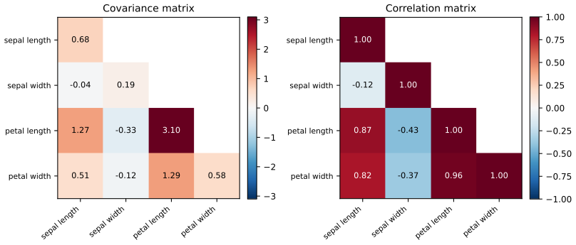
Figures and demonstrations. Every computed figure is reproduced by the Python code; two diagrams are redrawn. Data: Figure 4.1 uses the iris data; the polynomial examples use simulated data and Figure 4.8 uses a small digits classifier, as stated in the captions, because the book's own data sets are not available offline. The ▶ Demo boxes open an interactive demonstration set to the case being discussed.
Main reference
K. P. Murphy, Probabilistic Machine Learning: An Introduction, MIT Press (2022), Chapter 4, pages 107–166 (book page: probml.github.io/pml-book/book1.html). Section, equation, figure and exercise numbers below refer to this book. The explanations, derivations, figures and code are my own.
Companion courses
Much of this chapter is also developed, in other notation, elsewhere on this site. Where a result is proved in full there, these notes give the statement and a short sketch and link to it.
- Bayesian and Probabilistic Machine Learning (Bishop): 2.1 binary variables and the beta distribution, 2.2 multinomial variables and the Dirichlet, 2.3.4 maximum likelihood for the Gaussian, 2.3.6 Bayesian inference for the Gaussian, 3.1.4 regularised least squares, 3.2 bias–variance, 10.4 exponential-family approximations.
- All of Statistics (Wasserman): 9.3 maximum likelihood, 9.7 asymptotic normality, 9.8 optimality, 8.3 bootstrap intervals, 11.2 the Bayesian method.
- The first-year notes on estimation for the same ideas at an introductory level.
What this chapter adds: the ERM and surrogate-loss view, the online estimators, shrinkage covariance estimation, the one-standard-error rule, mixtures of conjugate priors, grid and Laplace posteriors, and the pitfalls of confidence intervals.
The chapter at a glance
- 4.2 MLE minimises the KL divergence to the empirical distribution (Result 4.1); closed forms for the Bernoulli, categorical, Gaussian (gap 4.2) and multivariate Gaussian.
- 4.3–4.4 Other losses and estimators: surrogate losses (Result 4.2), method of moments, running averages with bias correction (gap 4.4).
- 4.5 Regularisation = MAP: add-one smoothing, covariance shrinkage (gap 4.5), ridge, validation and cross-validation with a closed-form leave-one-out error (Result 4.3).
- 4.6 Bayesian inference: conjugate beta, Dirichlet and Gaussian updates, predictive distributions, marginal likelihood, mixtures of priors, credible and HPD intervals, grid and Laplace approximations.
- 4.7 Frequentist inference: Fisher information, asymptotic normality, bootstrap, confidence intervals and why they are not credible intervals, MSE = bias² + variance, shrinkage versus the MLE.
Notation. Data \(\mathcal D=\{y_n\}_{n=1}^N\) (or pairs \((\bm x_n,y_n)\)), parameter \(\theta\), \(\operatorname{NLL}(\theta)=-\log p(\mathcal D\given\theta)\). Hats denote estimates; \(\bar y\) is the sample mean. \(\operatorname{Beta}(a,b)\), \(\operatorname{Dir}(\bm\alpha)\), \(\mathcal N(\mu,\sigma^2)\) have the usual densities.
Prerequisites. The probability distributions of Chapters 2 and 3 of the book (Gaussian conditioning, the exponential family) and basic calculus and linear algebra.
4.1 Introduction
p. 107 Fitting a model means solving an optimisation problem \[ \hat{\bm\theta}=\argmin_{\bm\theta}\mathcal L(\bm\theta), \tag{4.1} \] with a loss or objective \(\mathcal L\). Beyond the point estimate we want to quantify uncertainty about it; the Bayesian way (Section 4.6) uses a posterior distribution, the frequentist way (Section 4.7) the sampling distribution of the estimator. In deep learning "inference" often means prediction; here it means learning about parameters.
4.2 Maximum likelihood estimation (MLE)
4.2.1 Definition
pp. 107–108 The maximum likelihood estimate is \[ \hat{\bm\theta}_{\rm mle}\triangleq\argmax_{\bm\theta}p(\mathcal D\given\bm\theta). \tag{4.2} \] Under the iid assumption the likelihood factorises, \(p(\mathcal D\given\bm\theta)=\prod_np(y_n\given\bm x_n,\bm\theta)\) (4.3), so the log-likelihood is a sum over examples (4.4)–(4.5), and minimising the negative log-likelihood \[ \operatorname{NLL}(\bm\theta)\triangleq-\sum_{n=1}^N\log p(y_n\given\bm x_n,\bm\theta) \tag{4.6} \] gives the same estimate. For an unconditional model drop \(\bm x_n\) (4.7); to model inputs too use \(p(y_n,\bm x_n\given\bm\theta)\) (4.8).
See also (companion): All of Statistics, 9.3 maximum likelihood.
4.2.2 Justification for MLE
pp. 108–110 Two justifications. First, MLE is MAP under a uniform prior: \(\hat{\bm\theta}_{\rm map}=\argmax_{\bm\theta}\{\log p(\mathcal D\given\bm\theta)+\log p(\bm\theta)\}\) (4.9). Second, it makes the model distribution as close as possible, in KL divergence, to the empirical distribution \(p_{\mathcal D}(y)=\frac1N\sum_n\delta(y-y_n)\) (4.10).
Result 4.1 (MLE minimises the KL divergence to the data) pp. 108–110, (4.11)–(4.19)
Let \(q(y)=p(y\given\bm\theta)\). For discrete \(y\),\[ D_{\rm KL}(p_{\mathcal D}\,\|\,q)=-H(p_{\mathcal D})-\frac1N\sum_n\log p(y_n\given\bm\theta), \tag{4.15}\]where \(H(p_{\mathcal D})\) does not depend on \(\bm\theta\). Hence \(\argmin_\theta D_{\rm KL}(p_{\mathcal D}\|q_\theta)=\argmin_\theta\operatorname{NLL}(\theta)\). In the conditional case, with \(p_{\mathcal D}(\bm x,y)=\frac1N\sum_n\delta(\bm x-\bm x_n)\delta(y-y_n)\), \[ \E_{p_{\mathcal D}(\bm x)}\big[D_{\rm KL}(p_{\mathcal D}(Y\given\bm x)\|q(Y\given\bm x))\big]=\mathrm{const}-\frac1N\sum_{n=1}^N\log p(y_n\given\bm x_n,\bm\theta). \tag{4.19} \] Moreover \(D_{\rm KL}(p\|q)\ge0\) with equality iff \(p=q\).
Proof
By definition (4.11), \(D_{\rm KL}(p\|q)=\sum_yp(y)\log\frac{p(y)}{q(y)}\), which splits as \(-H(p)+H_{\rm ce}(p,q)\) (4.12) with \(H_{\rm ce}(p,q)=-\sum_yp\log q\). With \(p=p_{\mathcal D}\), \(\sum_yp_{\mathcal D}(y)\log q(y)=\frac1N\sum_n\log q(y_n)\) because \(p_{\mathcal D}\) puts mass \(1/N\) on each \(y_n\) (4.13)–(4.15); with ties the masses add, with the same result. The conditional case (4.16)–(4.19) is the same computation with the weights \(p_{\mathcal D}(\bm x,y)\), using \(p_{\mathcal D}(y\given\bm x)p_{\mathcal D}(\bm x)=p_{\mathcal D}(\bm x,y)\).
Non-negativity (Gibbs' inequality). Since \(\log t\le t-1\) with equality iff \(t=1\), \(-D_{\rm KL}(p\|q)=\sum_{y:p>0}p\log\frac{q}{p}\le\sum_{y:p>0}p\big(\frac qp-1\big)=\sum_{y:p>0}q-1\le0\), with equality in the first step iff \(q=p\) wherever \(p>0\), and in the last iff \(q\) has no mass elsewhere. \(\square\)
See also (companion): Bayesian and Probabilistic ML, Section 1.6 (relative entropy and mutual information); Chapter 6 of this course for the KL divergence.
4.2.3 Example: MLE for the Bernoulli distribution
p. 110 With \(N_1\) heads and \(N_0\) tails, \(\operatorname{NLL}(\theta)=-[N_1\log\theta+N_0\log(1-\theta)]\) (4.20)–(4.23). Then \(\frac{d}{d\theta}\operatorname{NLL}=-\frac{N_1}\theta+\frac{N_0}{1-\theta}\) (4.24), which vanishes at \[ \hat\theta_{\rm mle}=\frac{N_1}{N_0+N_1}. \tag{4.25} \] The pair \((N_1,N_0)\) is a sufficient statistic: the likelihood depends on the data only through it. The NLL is strictly convex (second derivative \(N_1/\theta^2+N_0/(1-\theta)^2>0\)) so the stationary point is the global minimum when \(N_1,N_0>0\); if \(N_1=0\) the infimum \(\hat\theta=0\) is at the boundary.
4.2.4 Example: MLE for the categorical distribution
p. 111 \(\operatorname{NLL}(\bm\theta)=-\sum_kN_k\log\theta_k\) (4.26) subject to \(\sum_k\theta_k=1\). The Lagrangian (4.27), \(\mathcal L=-\sum_kN_k\log\theta_k-\lambda(1-\sum_k\theta_k)\), gives \(N_k=\lambda\theta_k\) (4.29), and summing, \(\lambda=N\), so \[ \hat\theta_k=\frac{N_k}N. \tag{4.31} \]
Filling the gap 4.1: why the stationary point is the global minimum, and footnote 3 p. 111
Derivation
The book only finds a stationary point. By Gibbs' inequality (Result 4.1) applied to the distributions \(\hat\theta=(N_k/N)_k\) and \(\bm\theta\): \(\sum_k\frac{N_k}N\log\frac{N_k/N}{\theta_k}\ge0\), i.e. \(-\sum_kN_k\log\theta_k\ge-\sum_kN_k\log(N_k/N)\) for every \(\bm\theta\) in the simplex, with equality iff \(\bm\theta=\hat{\bm\theta}\). So \(\hat{\bm\theta}\) is the unique global minimiser, including when some \(N_k=0\) (the terms \(0\log0\) are taken as \(0\)). The non-negativity constraint \(\theta_k\ge0\) needs no multiplier: the proof never used one, which is the content of footnote 3. The same argument covers the Bernoulli case.
4.2.5 Example: MLE for the univariate Gaussian
pp. 111–112 For \(y_n\overset{\rm iid}\sim\mathcal N(\mu,\sigma^2)\), \[ \operatorname{NLL}(\mu,\sigma^2)=\frac1{2\sigma^2}\sum_{n=1}^N(y_n-\mu)^2+\frac N2\log(2\pi\sigma^2), \tag{4.33} \] and the stationary point is \[ \hat\mu_{\rm mle}=\frac1N\sum_ny_n=\bar y,\qquad\hat\sigma^2_{\rm mle}=\frac1N\sum_n(y_n-\hat\mu)^2=s^2-\bar y^2,\quad s^2\triangleq\frac1N\sum_ny_n^2. \tag{4.35, 4.36} \] The sufficient statistics are \((\bar y,s^2)\). The divisor \(N-1\) of (4.38) is not the MLE but the unbiased estimator (Section 4.7.6.1).
Filling the gap 4.2: Exercise 4.1, the Gaussian MLE in full p. 112, p. 164
Derivation
Mean. \(\partial_\mu\operatorname{NLL}=-\frac1{\sigma^2}\sum_n(y_n-\mu)=0\Rightarrow\mu=\bar y\), for every \(\sigma^2\).
Variance. Write \(v=\sigma^2\). \(\partial_v\operatorname{NLL}=-\frac1{2v^2}\sum_n(y_n-\mu)^2+\frac N{2v}=0\Rightarrow v=\frac1N\sum_n(y_n-\mu)^2\). Substituting \(\mu=\bar y\) gives (4.36); the identity \(\frac1N\sum(y_n-\bar y)^2=s^2-\bar y^2\) follows by expanding the square and using \(\sum y_n=N\bar y\).
It is the global minimum. For fixed \(v\) the NLL is a convex quadratic in \(\mu\), minimised at \(\bar y\). Plugging in, \(\operatorname{NLL}(\bar y,v)=\frac{NS}{2v}+\frac N2\log v+\mathrm{const}\) with \(S=\frac1N\sum(y_n-\bar y)^2\). Its derivative in \(v\) is \(\frac N2\big(\frac1v-\frac S{v^2}\big)\), negative for \(v<S\) and positive for \(v>S\) (when \(S>0\)), so \(v=S\) is the global minimiser. If all \(y_n\) coincide, \(S=0\) and the NLL \(\to-\infty\) as \(v\to0\): the MLE does not exist (the likelihood is unbounded), a first sign of the overfitting discussed in Section 4.5. \(\square\)
4.2.6 Example: MLE for the multivariate Gaussian
pp. 112–114 With the precision \(\Lambda=\Sigma^{-1}\),\[ \ell(\bm\mu,\Lambda)=\frac N2\log|\Lambda|-\frac12\sum_n(\bm y_n-\bm\mu)^\T\Lambda(\bm y_n-\bm\mu). \tag{4.39}\] The maximisers are the empirical mean and the empirical covariance: \[ \hat{\bm\mu}=\bar{\bm y},\qquad\hat\Sigma=\frac1N\sum_n(\bm y_n-\bar{\bm y})(\bm y_n-\bar{\bm y})^\T=\frac1N\bm Y^\T\bm C_N\bm Y, \tag{4.43, 4.51} \] where \(\bm C_N=\bm I-\frac1N\bm 1\bm 1^\T\) is the centring matrix (4.48). The correlation matrix is \(\operatorname{corr}=\operatorname{diag}(\Sigma)^{-1/2}\Sigma\operatorname{diag}(\Sigma)^{-1/2}\) (4.52).
Filling the gap 4.3: the Gaussian MLE of mean and covariance, derived with the trace trick pp. 112–114, (4.40)–(4.51)
Derivation
Mean. The map \(\bm\mu\mapsto(\bm y_n-\bm\mu)^\T\Sigma^{-1}(\bm y_n-\bm\mu)\) has gradient \(-2\Sigma^{-1}(\bm y_n-\bm\mu)\) (for symmetric \(\Sigma^{-1}\); the book's (4.41) writes the same thing as \(-(\Sigma^{-1}+\Sigma^{-\T})\bm z_n\)). Setting the sum to zero, \(\Sigma^{-1}\sum_n(\bm y_n-\bm\mu)=0\), and since \(\Sigma^{-1}\) is invertible, \(\bm\mu=\bar{\bm y}\), whatever \(\Sigma\) is.
Covariance. Use \(\bm z^\T\Lambda\bm z=\operatorname{tr}(\Lambda\bm z\bm z^\T)\), so \(\ell(\bar{\bm y},\Lambda)=\frac N2\log|\Lambda|-\frac12\operatorname{tr}(\bm S\Lambda)\), with the scatter matrix \(\bm S=\sum_n(\bm y_n-\bar{\bm y})(\bm y_n-\bar{\bm y})^\T=\bm Y^\T\bm C_N\bm Y\) (4.45)–(4.47). The gradient is \(\frac N2\Lambda^{-1}-\frac12\bm S\) (symmetric matrices), which vanishes at \(\Lambda^{-1}=\bm S/N\) (4.50).
Global maximum. If \(\bm S\succ0\) (which needs \(N>D\) and the points not in a proper affine subspace), the map is concave in \(\Lambda\) on the positive definite cone because \(\log|\Lambda|\) is concave and the trace term is linear; a stationary point of a concave function is the global maximum. Alternatively, with eigenvalues \(\lambda_i\) of \(\bm S^{1/2}\Lambda\bm S^{1/2}\), \(\ell=\frac N2\sum_i\log\lambda_i-\frac12\sum_i\lambda_i-\frac N2\log|\bm S|\), maximised coordinate-wise at \(\lambda_i=N\). If \(N\le D\) then \(\bm S\) is singular (rank at most \(N-1\)) and the likelihood is unbounded: no MLE exists, which motivates Section 4.5.2. \(\square\)
See also (companion): Section 2.3.4, maximum likelihood for the Gaussian, including the bias of \(\hat\Sigma\).
4.2.7 Example: MLE for linear regression
pp. 114–115 For \(p(y\given\bm x;\bm\theta)=\mathcal N(y\given\bm w^\T\bm x,\sigma^2)\) (4.53) the NLL is, up to constants, \(\frac1{2\sigma^2}\operatorname{RSS}(\bm w)\) with \(\operatorname{RSS}(\bm w)=\sum_n(y_n-\bm w^\T\bm x_n)^2=\|\bm X\bm w-\bm y\|_2^2\) (4.55), (4.58). MSE and RMSE (4.56)–(4.57) are monotone rescalings of it and have the same minimiser, the ordinary least squares estimate \[ \hat{\bm w}_{\rm mle}=(\bm X^\T\bm X)^{-1}\bm X^\T\bm y. \tag{4.59} \]
Filling the gap 4.3b: the normal equations (proved in Section 11.2.2.1 of the book) p. 115
Derivation
\(\operatorname{RSS}(\bm w)=\bm w^\T\bm X^\T\bm X\bm w-2\bm w^\T\bm X^\T\bm y+\bm y^\T\bm y\) is a quadratic with gradient \(2\bm X^\T(\bm X\bm w-\bm y)\) and Hessian \(2\bm X^\T\bm X\succeq0\), hence convex. Minimisers are exactly the solutions of \(\bm X^\T\bm X\bm w=\bm X^\T\bm y\). If \(\bm X\) has full column rank, \(\bm X^\T\bm X\succ0\) is invertible and the unique solution is (4.59); the NLL depends on \(\sigma^2\) only through the factor \(1/(2\sigma^2)\), so \(\hat{\bm w}\) does not. (In practice solve by QR or SVD instead of forming the inverse.) The full treatment, including the rank-deficient case, is in the companion course.
4.3 Empirical risk minimization (ERM)
p. 115 Replace the log loss by any loss \(\ell\): \[ \mathcal L(\bm\theta)=\frac1N\sum_{n=1}^N\ell(y_n,\bm\theta;\bm x_n). \tag{4.60} \] This is the expected loss under the empirical distribution (Chapter 5).
4.3.1 Example: minimizing the misclassification rate
p. 116 The 0-1 loss is \(\ell_{01}=\mathbb I(y_n\ne f(\bm x_n;\bm\theta))\) (4.61), whose average is the training misclassification rate (4.62). With labels \(\tilde y\in\{-1,+1\}\) and prediction \(\hat y\), \(\ell_{01}(\tilde y,\hat y)=\mathbb I(\tilde y\hat y<0)\) (4.63)–(4.64).
4.3.2 Surrogate loss
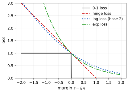
pp. 116–117 The 0-1 loss is a step function of the margin \(z=\tilde y\eta\), with zero gradient almost everywhere, and minimising it is NP-hard in general. A surrogate is a convex upper bound. The logistic model \(p(\tilde y\given\eta)=\sigma(\tilde y\eta)\) (4.65) has the log loss \(\ell_{\rm ll}(\tilde y,\eta)=\log(1+e^{-\tilde y\eta})\) (4.66); the hinge loss is \(\ell_{\rm hinge}=(1-\tilde y\eta)_+\) (4.67); the exponential loss is \(e^{-z}\).
Result 4.2 (surrogate losses) p. 116, Figure 4.2
(a) The hinge loss \(\max(0,1-z)\), the exponential loss \(e^{-z}\) and the base-2 log loss \(\log_2(1+e^{-z})\) are convex in \(z\) and bound \(\mathbb I(z<0)\) from above. (b) The natural-log loss (4.66) is not an upper bound: at \(z=0\) it equals \(\ln2\approx0.693<1=\ell_{01}(0)\) (the convention \(\ell_{01}(0)=1\), a prediction exactly on the boundary counted as an error). It is bounded below by the rescaled \(\ell_{01}\), namely \(\ln(1+e^{-z})\ge(\ln2)\,\mathbb I(z\le0)\), so minimising the NLL still controls the 0-1 loss up to the factor \(\ln2\).
Proof
Convexity: \(\max(0,1-z)\) is a maximum of affine functions; \(e^{-z}\) has second derivative \(e^{-z}>0\); \(\frac{d^2}{dz^2}\ln(1+e^{-z})=\sigma(z)\sigma(-z)>0\). Bounds: for \(z\ge0\) all three losses are \(\ge0=\ell_{01}\). For \(z<0\) we need \(\ge1\): hinge \(1-z>1\); exponential \(e^{-z}>1\); and \(\log_2(1+e^{-z})>\log_22=1\). For (b), \(\ln(1+e^{-z})\) is decreasing, so for \(z\le0\) it is \(\ge\ln(1+e^0)=\ln2\). \(\square\)
See also: Chapter 10 of the book (logistic regression) and Chapter 17 (SVMs, the hinge loss) in this course; ESL for the margin view of boosting and SVMs.
4.4 Other estimation methods
4.4.1 The method of moments
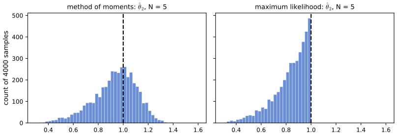
pp. 117–118 Solve \(\mu_k(\bm\theta)=\hat\mu_k\), \(k=1,\dots,K\) with \(\hat\mu_k=\frac1N\sum_ny_n^k\) (4.68). For the Gaussian the result equals the MLE (4.69)–(4.70). For \(\operatorname{Unif}(\theta_1,\theta_2)\), \(\mu_1=\frac12(\theta_1+\theta_2)\), \(\mu_2=\frac13(\theta_1^2+\theta_1\theta_2+\theta_2^2)\) (4.72)–(4.73) and \[ (\hat\theta_1,\hat\theta_2)=\big(\hat\mu_1-\sqrt{3(\hat\mu_2-\hat\mu_1^2)},\;2\hat\mu_1-\hat\theta_1\big). \tag{4.74} \] For \(\mathcal D=\{0,0,0,0,1\}\) this gives \((-0.493,0.893)\), impossible since the sample contains 1. The MLE is \((y_{(1)},y_{(N)})\) (4.77).
Filling the gap 4.4a: inverting the uniform moments and the uniform MLE pp. 117–118
Derivation
Put \(m=\mu_1=\frac12(\theta_1+\theta_2)\) and \(h=\frac12(\theta_2-\theta_1)\). Then \(\mu_2-\mu_1^2=\operatorname{var}(Y)=\frac{(\theta_2-\theta_1)^2}{12}=\frac{h^2}3\), so \(h=\sqrt{3(\mu_2-\mu_1^2)}\), \(\theta_1=m-h\), \(\theta_2=m+h=2m-\theta_1\): this is (4.74). It is an estimate that can place the interval so that sample points fall outside it, since nothing in the equations forces \([\hat\theta_1,\hat\theta_2]\supseteq[y_{(1)},y_{(N)}]\). Here \(\hat\mu_1=\hat\mu_2=\frac15\), \(h=\sqrt{3(\frac15-\frac1{25})}=\sqrt{0.48}=0.693\), reproducing \(-0.493\) and \(0.893\).
MLE. The likelihood is \((\theta_2-\theta_1)^{-N}\mathbb I(\theta_1\le y_{(1)})\mathbb I(y_{(N)}\le\theta_2)\) (4.75). On the feasible set it is strictly decreasing in the width \(\theta_2-\theta_1\) (4.76), so the maximum is at the narrowest feasible interval, \([y_{(1)},y_{(N)}]\) (4.77). Both estimators are consistent; the MLE converges at rate \(1/N\), the moment estimator only at \(1/\sqrt N\). Supplementary Figure 4.S3 shows the sampling distribution of \(\hat\theta_2\) for each.
4.4.2 Online (recursive) estimation
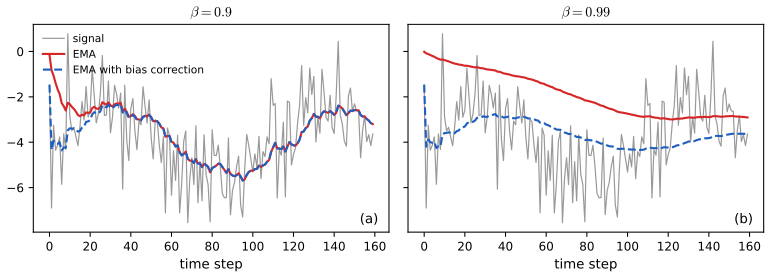
pp. 119–120 In a stream we want updates of constant cost, \(\hat\theta_t=f(\hat\theta_{t-1},y_t)\) (4.78). For the Gaussian mean, \[ \hat\mu_t=\frac1t\Big((t-1)\hat\mu_{t-1}+y_t\Big)=\hat\mu_{t-1}+\frac1t(y_t-\hat\mu_{t-1}), \tag{4.80, 4.81} \] a running average: old estimate plus a correction whose size shrinks like \(1/t\). To track a changing signal use the exponentially weighted moving average \[ \hat\mu_t=\beta\hat\mu_{t-1}+(1-\beta)y_t,\qquad0<\beta<1, \tag{4.82} \] which expands to \(\hat\mu_t=\beta^ty_0+(1-\beta)\sum_{k=0}^{t-1}\beta^ky_{t-k}\) (4.85).
Filling the gap 4.4: the geometric sum and the bias correction (4.86)–(4.88) p. 120
Derivation
Unrolling (4.82) from \(\hat\mu_0=0\): \(\hat\mu_t=(1-\beta)\sum_{k=1}^t\beta^{t-k}y_k\). The weights are \(w_k=(1-\beta)\beta^{t-k}\) and sum to \((1-\beta)\frac{1-\beta^t}{1-\beta}=1-\beta^t\) by the geometric sum (4.86)–(4.87) (the book writes the sum with one more term, which changes only the bookkeeping of the index of \(\hat\mu_0\)). So the weights do not sum to 1: if the signal is constant, \(y_k\equiv c\), then \(\hat\mu_t=(1-\beta^t)c\), a downward bias that decays only as \(\beta^t\) (slowly when \(\beta=0.99\)). Dividing by the total weight, \[ \tilde\mu_t=\frac{\hat\mu_t}{1-\beta^t}, \tag{4.88} \] turns the weights into a proper average, and removes the bias exactly for a constant signal. More generally \(\E[\tilde\mu_t]\) is a weighted average of \(\E[y_k]\). The uncorrected recursion keeps running on \(\hat\mu_{t-1}\); the correction is applied only to the output. The memory of the filter is about \(1/(1-\beta)\) steps (the mean age of the weights is \(\sum_jj\,\beta^j(1-\beta)=\beta/(1-\beta)\)). Figure 4.3 shows \(\beta=0.9\) and \(0.99\).
4.5 Regularization
pp. 120–121 MLE and ERM pick the parameters that fit the training set best, which may generalise badly: after three heads in three tosses \(\hat\theta_{\rm mle}=1\) and tails are declared impossible. The remedy is a penalty, \[ \mathcal L(\bm\theta;\lambda)=\Big[\frac1N\sum_n\ell(y_n,\bm\theta;\bm x_n)\Big]+\lambda C(\bm\theta),\qquad\lambda\ge0. \tag{4.89} \] With the log loss and \(C(\bm\theta)=-\log p(\bm\theta)\), \(\lambda=1/N\) after rescaling, minimising it is MAP estimation, \(\hat{\bm\theta}=\argmax\{\log p(\mathcal D\given\bm\theta)+\log p(\bm\theta)\}\) (4.91)–(4.92).
4.5.1 Example: MAP estimation for the Bernoulli distribution
pp. 121–122 With a \(\operatorname{Beta}(a,b)\) prior, \[ \hat\theta_{\rm map}=\frac{N_1+a-1}{N_1+N_0+a+b-2}, \tag{4.95} \] and for \(a=b=2\), \(\hat\theta=\frac{N_1+1}{N_1+N_0+2}\), add-one smoothing (4.96).
Filling the gap 4.5a: the MAP of the Bernoulli, and its limits p. 121
Derivation
\(\log p(\theta\given\mathcal D)=(N_1+a-1)\log\theta+(N_0+b-1)\log(1-\theta)+\mathrm{const}\) (4.94). If \(N_1+a>1\) and \(N_0+b>1\), this is strictly concave with derivative \(\frac{N_1+a-1}\theta-\frac{N_0+b-1}{1-\theta}\), vanishing at (4.95). If \(a=b=1\) it reduces to the MLE (4.25). If, say, \(N_1+a\le1\), the density increases to \(\theta=0\): the posterior has no interior mode (the mode is on the boundary). For \(a=b=2\) the prior is mildly peaked at \(\tfrac12\) and the formula is (4.96). The pseudo-counts \(a-1,b-1\) are fake observations added to \(N_1,N_0\). Note the distinction with Section 4.6.2.9: Laplace's rule \((N_1+1)/(N+2)\) arises from the posterior mean under the uniform prior, not the MAP.
4.5.2 Example: MAP estimation for the multivariate Gaussian
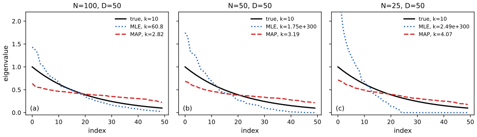
pp. 122–123 In high dimensions \(\hat\Sigma_{\rm mle}\) is singular if \(N<D\) and ill-conditioned otherwise. An inverse-Wishart prior with prior scatter \(\breve{\bm S}\) and prior sample size \(\breve N\) gives the shrinkage estimate \[ \hat\Sigma_{\rm map}=\frac{\breve{\bm S}+\bm S_y}{\breve N+N}=\lambda\Sigma_0+(1-\lambda)\hat\Sigma_{\rm mle},\qquad\lambda=\frac{\breve N}{\breve N+N},\ \Sigma_0=\breve{\bm S}/\breve N. \tag{4.97} \] With \(\breve{\bm S}=\breve N\operatorname{diag}(\hat\Sigma_{\rm mle})\) the diagonal stays at its MLE and each off-diagonal entry is multiplied by \((1-\lambda)\) (4.98). The data-driven choice of \(\lambda\) minimising expected squared Frobenius loss is the Ledoit–Wolf formula.
Filling the gap 4.5: the inverse-Wishart MAP (4.97), and why shrinkage fixes conditioning p. 122
Derivation
MAP. The inverse-Wishart density with scale matrix \(\bm\Psi\) and \(\nu\) degrees of freedom is \(\mathrm{IW}(\Sigma\given\bm\Psi,\nu)\propto|\Sigma|^{-(\nu+D+1)/2}\exp\{-\tfrac12\operatorname{tr}(\bm\Psi\Sigma^{-1})\}\). Multiplying by the Gaussian likelihood \(|\Sigma|^{-N/2}\exp\{-\frac12\operatorname{tr}(\bm S_y\Sigma^{-1})\}\) (the mean having been profiled out at \(\bar{\bm y}\)) gives a posterior of the same form, \(\mathrm{IW}(\bm\Psi+\bm S_y,\nu+N)\). The maximiser of \(|\Sigma|^{-m/2}\exp\{-\tfrac12\operatorname{tr}(\bm A\Sigma^{-1})\}\) is \(\Sigma=\bm A/m\) (the computation of Gap 4.3 with \(\Lambda=\Sigma^{-1}\)), so \[ \hat\Sigma_{\rm map}=\frac{\bm\Psi+\bm S_y}{\nu+D+1+N}. \] This equals the book's \((\breve{\bm S}+\bm S_y)/(\breve N+N)\) when \(\bm\Psi=\breve{\bm S}\) and \(\breve N=\nu+D+1\): the book's "prior sample size" is the degrees of freedom plus \(D+1\), not the degrees of freedom itself (a parametrisation to keep in mind when comparing with other texts). The convex-combination form follows by writing \(\breve{\bm S}+\bm S_y=\breve N\Sigma_0+N\hat\Sigma_{\rm mle}\).
Off-diagonal shrinkage. With \(\breve{\bm S}=\breve N\operatorname{diag}(\hat\Sigma)\), \(\Sigma_0=\operatorname{diag}(\hat\Sigma)\) and \(\hat\Sigma_{\rm map}=\lambda\operatorname{diag}(\hat\Sigma)+(1-\lambda)\hat\Sigma\): diagonal entries \(\hat\Sigma_{ii}\), off-diagonal \((1-\lambda)\hat\Sigma_{ij}\) (4.98).
Conditioning. \(\hat\Sigma_{\rm map}\) is a convex combination of the positive definite \(\Sigma_0\) and the positive semi-definite \(\hat\Sigma_{\rm mle}\), so \(\lambda_{\min}(\hat\Sigma_{\rm map})\ge\lambda\lambda_{\min}(\Sigma_0)>0\) whatever \(N\) and \(D\) are, and \(\lambda_{\max}\le\lambda\lambda_{\max}(\Sigma_0)+(1-\lambda)\lambda_{\max}(\hat\Sigma_{\rm mle})\). Thus the condition number is bounded, in contrast to the MLE (infinite for \(N\le D\)). Shrinkage changes eigenvalues, not eigenvectors, when the target is a multiple of the identity (the Ledoit–Wolf case); for the diagonal target of (4.98) eigenvectors do change a little. The Ledoit–Wolf intensity minimises \(\E\|\,(1-\delta)\hat\Sigma+\delta\mu\bm I-\Sigma\|_F^2\), a quadratic in \(\delta\), whose minimiser involves the unknown \(\|\Sigma-\mu\bm I\|_F^2\) and \(\E\|\hat\Sigma-\Sigma\|_F^2\); both are consistently estimated from the data, giving a closed form (implemented in the code, and equal to the scikit-learn estimate).
4.5.3 Example: weight decay
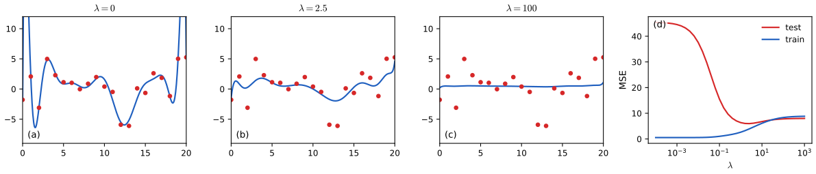
pp. 123–124 A zero-mean Gaussian prior on the weights gives \(\ell_2\) regularisation or weight decay, and for linear regression ridge regression: \[ \hat{\bm w}_{\rm map}=\argmin_{\bm w}\operatorname{NLL}(\bm w)+\lambda\|\bm w\|_2^2. \tag{4.99} \]
Filling the gap 4.6: ridge as MAP, its closed form, and shrinkage along singular directions p. 123
Derivation
With \(y_n\given\bm x_n\sim\mathcal N(\bm w^\T\bm x_n,\sigma^2)\) and \(\bm w\sim\mathcal N(0,\tau^2\bm I)\): \(-\log p(\bm w\given\mathcal D)=\frac1{2\sigma^2}\|\bm X\bm w-\bm y\|^2+\frac1{2\tau^2}\|\bm w\|^2+\mathrm{const}\). Multiplying by \(2\sigma^2\) gives \(\operatorname{RSS}(\bm w)+\lambda\|\bm w\|^2\) with \(\lambda=\sigma^2/\tau^2\) (in (4.99) the NLL is \(\operatorname{RSS}/(2\sigma^2)\), so its \(\lambda\) is \(1/(2\tau^2)\); the two conventions differ by a constant factor and the demo uses the RSS form). The gradient is \(2\bm X^\T(\bm X\bm w-\bm y)+2\lambda\bm w\) and the Hessian \(2(\bm X^\T\bm X+\lambda\bm I)\succ0\) for \(\lambda>0\), so there is a unique minimiser \[ \hat{\bm w}_\lambda=(\bm X^\T\bm X+\lambda\bm I)^{-1}\bm X^\T\bm y,\] which exists even when \(\bm X^\T\bm X\) is singular. With the SVD \(\bm X=\bm U\bm D\bm V^\T\), \(\hat{\bm w}_\lambda=\sum_i\frac{d_i}{d_i^2+\lambda}(\bm u_i^\T\bm y)\bm v_i\): the component along \(\bm v_i\) of the least-squares solution is multiplied by \(d_i^2/(d_i^2+\lambda)\in(0,1)\), shrinking most the directions with small singular values, those the data determine worst. The full discussion is in the companion course, Section 3.1.4, and in Chapter 11 of the book. An intercept is normally left unpenalised (centre \(\bm y\) and the columns of \(\bm X\)), as done in the code; a penalty on the other coefficients also depends on the feature scaling.
See also (companion): curve-fitting demo, regularised least squares; ESL Chapter 3.
4.5.4 Picking the regularizer using a validation set
pp. 124–125 Split the data into \(\mathcal D_{\rm train}\) and \(\mathcal D_{\rm valid}\). For each \(\lambda\) in a grid \(\mathcal S\) compute \(\hat{\bm\theta}_\lambda(\mathcal D_{\rm train})=\argmin R_\lambda(\bm\theta,\mathcal D_{\rm train})\) (4.102), the validation risk \(R^{\rm val}_\lambda=R_0(\hat{\bm\theta}_\lambda(\mathcal D_{\rm train}),\mathcal D_{\rm valid})\) (4.103), then \(\lambda^*=\argmin_{\lambda\in\mathcal S}R^{\rm val}_\lambda\) (4.104) and refit on all the data (4.105). The regularised empirical risk is \(R_\lambda(\bm\theta,\mathcal D)=\frac1{|\mathcal D|}\sum_{(\bm x,y)\in\mathcal D}\ell(y,f(\bm x;\bm\theta))+\lambda C(\bm\theta)\) (4.101); the validation risk uses \(\lambda=0\) because it estimates the population risk.
4.5.5 Cross-validation
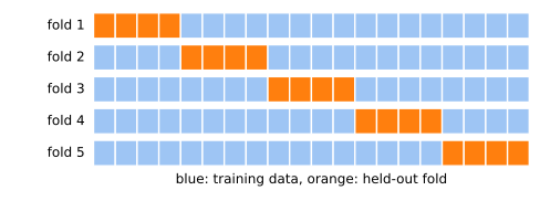
pp. 125–126 With little data, split into \(K\) folds (Figure 4.6) and average the held-out risks: \[ R^{\rm cv}_\lambda=\frac1K\sum_{k=1}^KR_0\big(\hat{\bm\theta}_\lambda(\mathcal D_{-k}),\mathcal D_k\big). \tag{4.106} \] \(K=N\) is leave-one-out (LOO) cross-validation.
Result 4.3 (leave-one-out for ridge without refitting) p. 126 (Section 4.5.5)
Let \(\bm H=\bm X(\bm X^\T\bm X+\bm P)^{-1}\bm X^\T\) be the hat matrix of a ridge fit with penalty matrix \(\bm P\succeq0\) (for an unpenalised intercept, the first column of \(\bm X\) is ones and \(P_{11}=0\)). Then the leave-one-out residual is \(y_i-\hat y_{-i}=\dfrac{y_i-\hat y_i}{1-H_{ii}}\), so \(R^{\rm cv}_{\rm LOO}=\frac1N\sum_i\big(\frac{y_i-\hat y_i}{1-H_{ii}}\big)^2\): one fit gives all \(N\) held-out errors.
Proof
Let \(\bm A=\bm X^\T\bm X+\bm P\) and \(\hat{\bm w}=\bm A^{-1}\bm X^\T\bm y\). Removing row \(i\) changes \(\bm A\) to \(\bm A_{-i}=\bm A-\bm x_i\bm x_i^\T\) and \(\bm X^\T\bm y\) to \(\bm X^\T\bm y-\bm x_iy_i\). By Sherman–Morrison, \(\bm A_{-i}^{-1}=\bm A^{-1}+\frac{\bm A^{-1}\bm x_i\bm x_i^\T\bm A^{-1}}{1-h_i}\) with \(h_i=\bm x_i^\T\bm A^{-1}\bm x_i=H_{ii}\). Then \(\hat{\bm w}_{-i}=\bm A_{-i}^{-1}(\bm X^\T\bm y-\bm x_iy_i)=\hat{\bm w}-\bm A^{-1}\bm x_iy_i+\frac{\bm A^{-1}\bm x_i(\bm x_i^\T\hat{\bm w}-h_iy_i)}{1-h_i}=\hat{\bm w}-\frac{\bm A^{-1}\bm x_i(y_i-\hat y_i)}{1-h_i}.\) Hence \(\hat y_{-i}=\bm x_i^\T\hat{\bm w}_{-i}=\hat y_i-\frac{h_i(y_i-\hat y_i)}{1-h_i}\) and \(y_i-\hat y_{-i}=(y_i-\hat y_i)\big(1+\frac{h_i}{1-h_i}\big)=\frac{y_i-\hat y_i}{1-h_i}\). \(\square\)
4.5.5.1 The one standard error rule
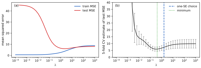
p. 126 Let \(L_n\) be the loss on example \(n\) when it is held out, \(\hat\mu=\frac1N\sum L_n\), \(\hat\sigma^2=\frac1N\sum(L_n-\hat\mu)^2\) and \(\operatorname{se}(\hat\mu)=\hat\sigma/\sqrt N\). The one-standard-error rule picks the simplest model (largest \(\lambda\)) whose CV risk is within one standard error of the best. Note that the standard error is the standard deviation of the sampling distribution of \(\hat\mu\), not its mean as the book's wording suggests; and treating the \(L_n\) as independent is an approximation, since they come from overlapping training sets.
4.5.5.2 Example: ridge regression
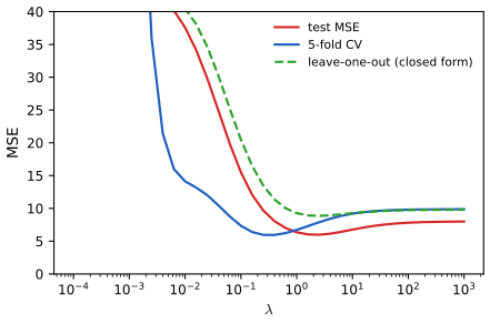
pp. 126–127 Figure 4.7 shows the training and test error against \(\lambda\) and the 5-fold CV estimate with its error bars. Test error is U-shaped; the CV curve has its minimum near the test minimum, but is higher at small \(\lambda\) because each fold trains on only 16 or 17 points. Supplementary Figure 4.S2 compares CV, the closed-form LOO of Result 4.3 and the test error.
4.5.6 Early stopping
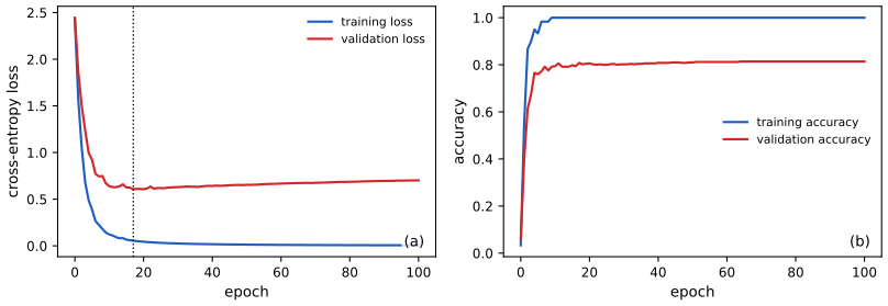
pp. 126–127 Because iterative optimisers move away from the initialisation gradually, stopping when the validation loss starts to rise limits the effective complexity. For quadratic losses, gradient descent started at 0 and stopped after \(t\) steps acts like ridge regression with \(\lambda\approx1/(\eta t)\), shrinking the same singular directions (see the deep learning course).
4.5.7 Using more data
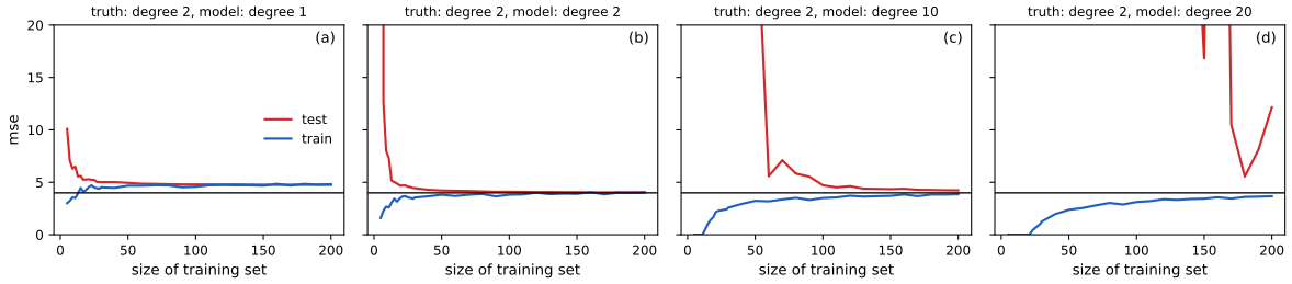
pp. 127–128 For a fixed model class the risk of overfitting falls as \(N\) grows. A learning curve plots train and test error against \(N\). Below, the truth is a quadratic with noise variance 4 (the noise floor, the Bayes error). The degree-1 model underfits (its test error stays above the floor), the others reach the floor, simpler ones faster; the train–test gap shrinks with \(N\); and the training error rises with \(N\) at first since there are more patterns to fit.
4.6 Bayesian statistics
pp. 129–153 Point estimates ignore how uncertain they are. The Bayesian treats \(\bm\theta\) as a random variable with a prior \(p(\bm\theta)\) and conditions on the data with Bayes' rule, \[ p(\bm\theta\given\mathcal D)=\frac{p(\bm\theta)p(\mathcal D\given\bm\theta)}{p(\mathcal D)}=\frac{p(\bm\theta)p(\mathcal D\given\bm\theta)}{\int p(\bm\theta')p(\mathcal D\given\bm\theta')\,d\bm\theta'}, \tag{4.107} \] where \(p(\mathcal D)\) is the marginal likelihood. Predictions integrate the parameters out, a form of Bayes model averaging: \[ p(y\given\bm x,\mathcal D)=\int p(y\given\bm x,\bm\theta)\,p(\bm\theta\given\mathcal D)\,d\bm\theta. \tag{4.108} \]
See also (companion): All of Statistics, 11.2 the Bayesian method.
4.6.1 Conjugate priors
pp. 129–130 A family \(\mathcal F\) of priors is conjugate to a likelihood if the posterior is in \(\mathcal F\) whenever the prior is. For exponential-family likelihoods there is always a conjugate prior whose hyperparameters act as pseudo-observations of the sufficient statistics (companion, Section 2.4.2).
4.6.2 The beta-binomial model
4.6.2.1–4.6.2.3 Likelihood and prior
p. 130 For \(y_n\sim\operatorname{Ber}(\theta)\) iid, \(p(\mathcal D\given\theta)=\theta^{N_1}(1-\theta)^{N_0}\) (4.109). A binomial observation \(y\sim\operatorname{Bin}(N,\theta)\) has likelihood \(\binom Ny\theta^y(1-\theta)^{N-y}\) (4.110), proportional in \(\theta\) to the Bernoulli one, so the posterior is the same. The prior \(p(\theta)\propto\theta^{\breve\alpha-1}(1-\theta)^{\breve\beta-1}\), \(\operatorname{Beta}(\breve\alpha,\breve\beta)\), is conjugate (4.111).
4.6.2.4–4.6.2.5 Posterior and example
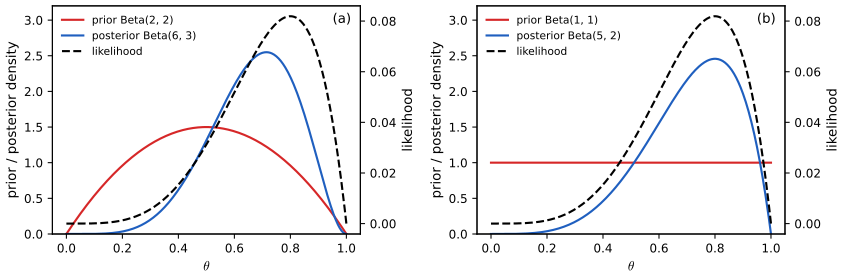
pp. 131–132 Multiplying, \[ p(\theta\given\mathcal D)\propto\theta^{N_1+\breve\alpha-1}(1-\theta)^{N_0+\breve\beta-1}=\operatorname{Beta}(\theta\given\hat\alpha,\hat\beta),\quad\hat\alpha=\breve\alpha+N_1,\ \hat\beta=\breve\beta+N_0. \tag{4.112--4.114} \] Prior counts add to data counts; \(\breve N=\breve\alpha+\breve\beta\) is the equivalent sample size. The posterior is a compromise between prior and likelihood (Figure 4.10); with \(\operatorname{Beta}(1,1)=\operatorname{Unif}(0,1)\) it has the shape of the likelihood.
4.6.2.6–4.6.2.8 Posterior mode, mean and variance
pp. 132–133 The mode (MAP) is \(\hat\theta_{\rm map}=\frac{\breve\alpha+N_1-1}{\breve\alpha+N_1-1+\breve\beta+N_0-1}\) (4.119), reducing to add-one smoothing for \(\operatorname{Beta}(2,2)\) (4.120) and to the MLE for the uniform prior (4.122). The mean is \(\bar\theta=\hat\alpha/\hat N\), \(\hat N=\hat\alpha+\hat\beta\) (4.123), a convex combination of the prior mean \(m=\breve\alpha/\breve N\) and the MLE: \[ \E[\theta\given\mathcal D]=\lambda m+(1-\lambda)\hat\theta_{\rm mle},\qquad\lambda=\frac{\breve N}{\hat N}. \tag{4.124} \] The variance is \[ \operatorname{var}[\theta\given\mathcal D]=\frac{\hat\alpha\hat\beta}{(\hat\alpha+\hat\beta)^2(\hat\alpha+\hat\beta+1)}=\E[\theta\given\mathcal D]^2\frac{\hat\beta}{\hat\alpha(1+\hat\alpha+\hat\beta)}, \tag{4.126} \] and for \(N\gg\breve N\), \(\operatorname{var}\approx\hat\theta(1-\hat\theta)/N\) (4.127), so the standard error decreases like \(1/\sqrt N\) (4.128).
Filling the gap 4.7: beta moments, the posterior mean as a shrinkage estimate, and the variance formula pp. 132–133, (4.119)–(4.128)
Derivation
Normalisation and moments. \(B(a,b)=\int_0^1\theta^{a-1}(1-\theta)^{b-1}d\theta=\Gamma(a)\Gamma(b)/\Gamma(a+b)\). Then \(\E[\theta^r]=B(a+r,b)/B(a,b)\), so \(\E\theta=\frac{\Gamma(a+1)\Gamma(a+b)}{\Gamma(a)\Gamma(a+b+1)}=\frac a{a+b}\) and \(\E\theta^2=\frac{a(a+1)}{(a+b)(a+b+1)}\). Hence \(\operatorname{var}=\frac{a(a+1)}{(a+b)(a+b+1)}-\frac{a^2}{(a+b)^2}=\frac{a[(a+1)(a+b)-a(a+b+1)]}{(a+b)^2(a+b+1)}=\frac{ab}{(a+b)^2(a+b+1)}\). The second form of (4.126) follows from \(\bar\theta^2=\hat\alpha^2/(\hat\alpha+\hat\beta)^2\).
Convex combination. \(\frac{\breve\alpha+N_1}{\breve N+N}=\frac{\breve N}{\breve N+N}\cdot\frac{\breve\alpha}{\breve N}+\frac{N}{\breve N+N}\cdot\frac{N_1}N\), and \(\breve N+N=\hat N\), which is (4.124).
Large-sample variance. If \(N\to\infty\) with \(N_1/N\to\hat\theta\), then \(\hat\alpha\hat\beta/\hat N^2\to\hat\theta(1-\hat\theta)\) and \(\hat N+1\sim N\), so \(\operatorname{var}\approx\hat\theta(1-\hat\theta)/N\), which is the Fisher-information variance of Section 4.7.2 (the Bernstein–von Mises phenomenon).
Where the uncertainty is largest. \(\hat\theta(1-\hat\theta)\) is maximal at \(\hat\theta=\tfrac12\) and shrinks near 0 or 1: it is easier to be sure that a coin is biased than that it is fair.
4.6.2.9 Posterior predictive
pp. 133–135 The plug-in approximation substitutes a point estimate \(p(y\given\hat\theta)\) and can overfit: after three heads \(\hat\theta_{\rm mle}=1\). Integrating over \(\theta\) for the Bernoulli, \[ p(y=1\given\mathcal D)=\int_0^1\theta\operatorname{Beta}(\theta\given\hat\alpha,\hat\beta)\,d\theta=\frac{\hat\alpha}{\hat\alpha+\hat\beta}, \tag{4.129--4.130} \] and with the uniform prior this is Laplace's rule of succession \(\frac{N_1+1}{N_1+N_0+2}\) (4.131). For the number \(y\) of heads in \(M\) future tosses, \[ p(y\given\mathcal D,M)=\operatorname{Bb}(y\given M,\hat\alpha,\hat\beta)=\binom My\frac{B(y+\hat\alpha,M-y+\hat\beta)}{B(\hat\alpha,\hat\beta)}. \tag{4.132--4.135} \]
Filling the gap 4.8: the beta-binomial predictive and its heavier tails pp. 134–135
Derivation
\(\int_0^1\binom My\theta^y(1-\theta)^{M-y}\frac{\theta^{\hat\alpha-1}(1-\theta)^{\hat\beta-1}}{B(\hat\alpha,\hat\beta)}d\theta=\binom My\frac{B(y+\hat\alpha,M-y+\hat\beta)}{B(\hat\alpha,\hat\beta)}\), since the integrand is, up to the constant, a \(\operatorname{Beta}(y+\hat\alpha,M-y+\hat\beta)\) density (4.134). Summing over \(y\) gives one (the pmf of a mixture of binomials). Mean and variance. By the laws of total expectation and variance with \(\bar\theta=\hat\alpha/\hat N\): \(\E y=M\bar\theta\) and \(\operatorname{var}y=\E[M\theta(1-\theta)]+\operatorname{var}(M\theta)=M\bar\theta(1-\bar\theta)\big(1+\frac{M-1}{\hat N+1}\big)\), where the last equality uses \(\operatorname{var}\theta=\bar\theta(1-\bar\theta)/(\hat N+1)\) and \(\E\theta(1-\theta)=\bar\theta(1-\bar\theta)\frac{\hat N}{\hat N+1}\). Compared with the plug-in binomial \(\operatorname{Bin}(M,\bar\theta)\), whose variance is \(M\bar\theta(1-\bar\theta)\), the predictive variance is larger by the factor \(1+\frac{M-1}{\hat N+1}\): parameter uncertainty adds variance, giving the longer tails of Figure 4.12 and avoiding black-swan type paradoxes. For \(M=1\) the two coincide at the posterior mean.
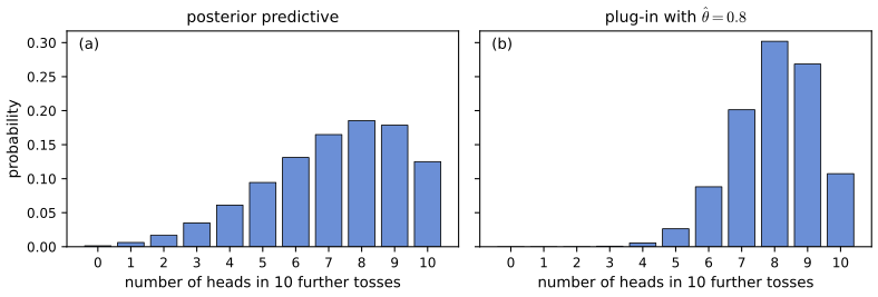
Figure 4.11 of the book (a tree of predictive probabilities under sequential updating, from Ortega et al.) is a diagram; the rule it illustrates is \(p(x_{t}=1\given h_t)=(N_{1,t}+1)/(t+2)\), which follows from (4.131).
4.6.2.10 Marginal likelihood
pp. 135–136 The evidence \(p(\mathcal D\given\mathcal M)=\int p(\bm\theta\given\mathcal M)p(\mathcal D\given\bm\theta,\mathcal M)\,d\bm\theta\) (4.138) is constant in \(\bm\theta\) but drives model comparison (Chapter 5) and empirical Bayes. For the beta-binomial model, \(p(\mathcal D)=\binom N{N_1}\frac{B(a+N_1,b+N_0)}{B(a,b)}\) (4.143); for the beta-Bernoulli model (a particular sequence) omit the binomial coefficient.
Filling the gap 4.9: the marginal likelihood as a ratio of normalisers p. 136, (4.139)–(4.143)
Derivation
Directly, \(p(\mathcal D)=\int_0^1\binom N{N_1}\theta^{N_1}(1-\theta)^{N_0}\frac{\theta^{a-1}(1-\theta)^{b-1}}{B(a,b)}d\theta=\binom N{N_1}\frac{B(a+N_1,b+N_0)}{B(a,b)}\) by the definition of the beta function. The book's route is Bayes' rule: both sides of \(p(\theta\given\mathcal D)=p(\mathcal D\given\theta)p(\theta)/p(\mathcal D)\) are densities in \(\theta\); matching the constant in front of \(\theta^{a+N_1-1}(1-\theta)^{b+N_0-1}\) gives \(1/B(a+N_1,b+N_0)=\binom N{N_1}\frac1{p(\mathcal D)B(a,b)}\), i.e. (4.142)–(4.143). For \(a=b=1\), \(p(\mathcal D)=\binom N{N_1}\frac{N_1!N_0!}{(N+1)!}=\frac1{N+1}\): every count is equally likely a priori. Sequentially, \(p(\mathcal D)=\prod_tp(y_t\given y_{1:t-1})\) with Laplace-type predictive factors; the code confirms this identity.
4.6.2.11 Mixtures of conjugate priors
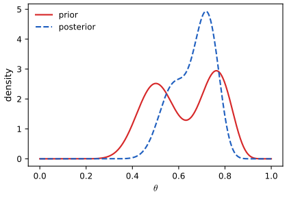
pp. 136–137 A single beta cannot express "the coin is fair or biased towards heads". A mixture \(p(\theta)=\sum_kp(h=k)p(\theta\given h=k)\) (4.145) is conjugate: the posterior is a mixture of the component posteriors with weights \[ p(h=k\given\mathcal D)=\frac{p(h=k)\,p(\mathcal D\given h=k)}{\sum_{k'}p(h=k')\,p(\mathcal D\given h=k')}, \tag{4.146--4.147} \] where \(p(\mathcal D\given h=k)\) is the marginal likelihood (4.143) of component \(k\). For the prior \(0.5\operatorname{Beta}(20,20)+0.5\operatorname{Beta}(30,10)\) (4.144) and \(N_1=20,N_0=10\), the posterior is \(0.346\operatorname{Beta}(40,30)+0.654\operatorname{Beta}(50,20)\) (4.148) and \(\Pr(\theta>0.5\given\mathcal D)=0.9604\) (4.149), against \(0.8858\) for the single \(\operatorname{Beta}(20,20)\) prior; both numbers were confirmed numerically.
Filling the gap 4.10: Exercise 4.6, a mixture of conjugate priors is conjugate p. 166
Proof
Let \(p(\theta)=\sum_kw_kp_k(\theta)\) with \(w_k=p(z=k)\) and each \(p_k\) conjugate. Then \(p(\theta\given\mathcal D)\propto p(\mathcal D\given\theta)\sum_kw_kp_k(\theta)=\sum_kw_k\,p(\mathcal D\given\theta)p_k(\theta)\). For each \(k\), \(p(\mathcal D\given\theta)p_k(\theta)=m_k\,p_k(\theta\given\mathcal D)\) where \(m_k=\int p(\mathcal D\given\theta)p_k(\theta)\,d\theta=p(\mathcal D\given z=k)\) is the marginal likelihood and \(p_k(\theta\given\mathcal D)\) is in the family by conjugacy. So \(p(\theta\given\mathcal D)\propto\sum_kw_km_kp_k(\theta\given\mathcal D)\), a mixture of members of the family; normalising, the weights are \(w_km_k/\sum_jw_jm_j\), which is (4.147). Equivalently, by Bayes' rule on the latent indicator, \(p(z=k\given\mathcal D)\propto p(z=k)p(\mathcal D\given z=k)\) and \(p(\theta\given\mathcal D,z=k)=p_k(\theta\given\mathcal D)\). The family of finite mixtures is therefore closed under updating, and by choosing enough components it can approximate any prior on \([0,1]\) arbitrarily well. For the example, the marginal likelihoods (4.143) of the two components are \(B(40,30)/B(20,20)\) and \(B(50,20)/B(30,10)\) (binomial coefficient cancels), whose ratio with equal prior weights yields the weights \(0.346\) and \(0.654\). \(\square\)
4.6.3 The Dirichlet-multinomial model
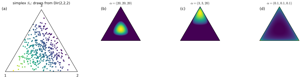
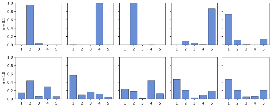
pp. 137–141 For \(Y\sim\operatorname{Cat}(\bm\theta)\) over \(C\) outcomes, \(p(\mathcal D\given\bm\theta)=\prod_c\theta_c^{N_c}\) (4.150). The conjugate prior is the Dirichlet on the simplex \(\mathcal S_K\) (4.151), \[ \operatorname{Dir}(\bm\theta\given\breve{\bm\alpha})=\frac1{B(\breve{\bm\alpha})}\prod_k\theta_k^{\breve\alpha_k-1},\qquad B(\bm\alpha)=\frac{\prod_k\Gamma(\alpha_k)}{\Gamma(\sum_k\alpha_k)}, \tag{4.152--4.153} \] whose total \(\breve\alpha_0=\sum\breve\alpha_k\) controls the concentration and whose ratios control the location (Figure 4.14); for \(\alpha_k<1\) it concentrates at the corners and samples are sparse (Figure 4.15). The posterior adds counts, \[ p(\bm\theta\given\mathcal D)=\operatorname{Dir}(\bm\theta\given\breve\alpha_1+N_1,\dots,\breve\alpha_K+N_K), \tag{4.154--4.157} \] with mean \(\bar\theta_k=\hat\alpha_k/\sum_{k'}\hat\alpha_{k'}\) (4.158) and mode \(\hat\theta_k=\frac{\hat\alpha_k-1}{\sum_{k'}(\hat\alpha_{k'}-1)}\) (4.159), which is the MLE \(N_k/N\) for the uniform prior (4.160). The posterior predictive is \(p(y=k\given\mathcal D)=\bar\theta_k\) (4.161)–(4.163), and the marginal likelihood is \[ p(\mathcal D)=\frac{B(\bm N+\bm\alpha)}{B(\bm\alpha)}=\frac{\Gamma(\sum_k\alpha_k)}{\Gamma(N+\sum_k\alpha_k)}\prod_k\frac{\Gamma(N_k+\alpha_k)}{\Gamma(\alpha_k)}. \tag{4.165--4.167} \]
Filling the gap 4.11: the Dirichlet normaliser, mode, predictive and marginal likelihood pp. 138–141
Derivation
Normalisation. The integral \(\int_{\mathcal S_K}\prod\theta_k^{\alpha_k-1}d\theta=B(\bm\alpha)\) follows by induction from the beta integral: write \(\theta_K=1-\sum_{k<K}\theta_k\) and substitute \(\theta_{K-1}=(1-\sum_{k<K-1}\theta_k)u\); the inner integral is \(B(\alpha_{K-1},\alpha_K)\) times a power of the remaining mass, and the Gamma functions telescope.
Posterior and predictive. The posterior kernel is \(\prod\theta_k^{N_k+\breve\alpha_k-1}\), a Dirichlet kernel (4.155). Since \(p(y=k\given\bm\theta)=\theta_k\), \(p(y=k\given\mathcal D)=\E[\theta_k\given\mathcal D]\), and \(\E\theta_k=B(\bm\alpha+\bm e_k)/B(\bm\alpha)=\alpha_k\Gamma(\alpha_0)/\Gamma(\alpha_0+1)=\alpha_k/\alpha_0\).
Mode. Maximise \(\sum_k(\hat\alpha_k-1)\log\theta_k\) on the simplex with a multiplier: \((\hat\alpha_k-1)/\theta_k=\lambda\), and normalising, \(\lambda=\sum_{k'}(\hat\alpha_{k'}-1)\). This is the interior mode when every \(\hat\alpha_k>1\); with some \(\hat\alpha_k<1\) the density is unbounded at a face. Add-one smoothing for the categorical needs \(\breve\alpha_k=2\) in the MAP, but \(\breve\alpha_k=1\) with the posterior mean.
Marginal likelihood. \(p(\mathcal D)=\int p(\mathcal D\given\bm\theta)\operatorname{Dir}(\bm\theta\given\bm\alpha)d\bm\theta=\frac{1}{B(\bm\alpha)}\int\prod\theta_k^{N_k+\alpha_k-1}d\bm\theta=\frac{B(\bm N+\bm\alpha)}{B(\bm\alpha)}\) (4.165); (4.167) is the same written with Gamma functions. It equals the product of sequential predictive probabilities \(\prod_t\hat\alpha^{(t-1)}_{y_t}/\hat\alpha_0^{(t-1)}\), which the code confirms, and implies the predictive for a batch (4.164) as the ratio of two marginal likelihoods.
4.6.4 The Gaussian-Gaussian model
4.6.4.1 Univariate case
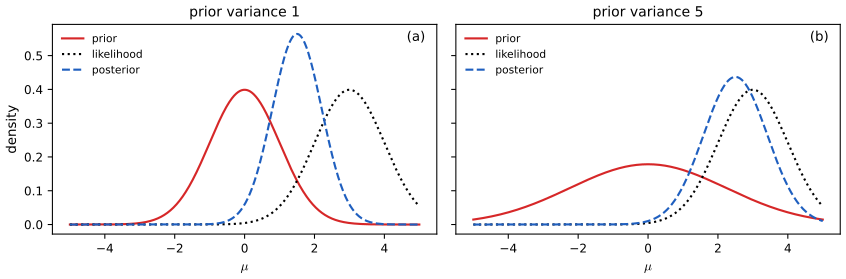
pp. 141–143 With known variance \(\sigma^2\), the likelihood in \(\mu\) is \(\propto\exp\{-\frac1{2\sigma^2}\sum_n(y_n-\mu)^2\}\) (4.168), and a \(\mathcal N(\breve m,\breve\tau^2)\) prior is conjugate. In terms of precisions \(\kappa=1/\sigma^2\) and \(\breve\lambda=1/\breve\tau^2\), \[ p(\mu\given\mathcal D,\sigma^2)=\mathcal N(\mu\given\hat m,\hat\lambda^{-1}),\qquad\hat\lambda=\breve\lambda+N\kappa,\qquad\hat m=\frac{N\kappa\bar y+\breve\lambda\breve m}{\hat\lambda}. \tag{4.169--4.174} \] Precisions add; the posterior mean is a convex combination of \(\bar y\) and \(\breve m\). For a single observation, with \(w=\breve\lambda/\hat\lambda\), \[ \hat m=\frac{\breve\lambda}{\hat\lambda}\breve m+\frac\kappa{\hat\lambda}y=\breve m+\frac\kappa{\hat\lambda}(y-\breve m)=y-w(y-\breve m)=(1-w)y+w\breve m \tag{4.175--4.178} \] (prior mean moved towards the data, or data shrunk towards the prior mean). The posterior mean equals the mode, so these formulae also give the MAP (Exercise 4.2). With the flat prior \(\breve\lambda=0\) and \(\sigma^2\) replaced by the sample variance \(s^2\), the standard error of the mean is \(\operatorname{se}(\mu)=s/\sqrt N\) (4.181) and the approximate 95% credible interval is \(\bar y\pm2s/\sqrt N\) (4.182).
Filling the gap 4.12: the Gaussian posterior by completing the square, and the multivariate case pp. 141–144, (4.169)–(4.189)
Derivation
Univariate. The log posterior is, up to a constant, \(-\frac\kappa2\sum_n(y_n-\mu)^2-\frac{\breve\lambda}2(\mu-\breve m)^2\). Expanding, the coefficient of \(\mu^2\) is \(-\frac12(N\kappa+\breve\lambda)\) and that of \(\mu\) is \(N\kappa\bar y+\breve\lambda\breve m\) (using \(\sum y_n=N\bar y\)). A function \(-\frac12\hat\lambda\mu^2+b\mu+c\) equals \(-\frac12\hat\lambda(\mu-b/\hat\lambda)^2+\mathrm{const}\), a Gaussian log-density with precision \(\hat\lambda=N\kappa+\breve\lambda\) and mean \(\hat m=b/\hat\lambda\): (4.172)–(4.174). The variance form (4.170) is \(\hat\tau^2=1/(N/\sigma^2+1/\breve\tau^2)=\sigma^2\breve\tau^2/(N\breve\tau^2+\sigma^2)\). The remaining forms of (4.175)–(4.178) are algebra: \(\breve m+\frac\kappa{\hat\lambda}(y-\breve m)=\frac{\hat\lambda-\kappa}{\hat\lambda}\breve m+\frac\kappa{\hat\lambda}y\), and \(\hat\lambda-\kappa=\breve\lambda\) for \(N=1\).
Sufficiency. Because \(\sum_n(y_n-\mu)^2=\sum_n(y_n-\bar y)^2+N(\bar y-\mu)^2\), the likelihood in \(\mu\) is that of a single observation \(\bar y\) with precision \(N\kappa\), which is (4.185): \(N\) measurements of precision \(\kappa\) count as one of value \(\bar y\) and precision \(N\kappa\).
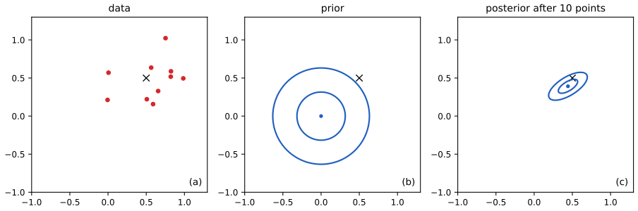
Multivariate. The same completion with matrices: the log posterior is \(-\frac12\bm\mu^\T(\breve{\bm V}^{-1}+N\Sigma^{-1})\bm\mu+\bm\mu^\T(\Sigma^{-1}N\bar{\bm y}+\breve{\bm V}^{-1}\breve{\bm m})+\mathrm{const}\), hence \(\hat{\bm V}^{-1}=\breve{\bm V}^{-1}+N\Sigma^{-1}\) and \(\hat{\bm m}=\hat{\bm V}(\Sigma^{-1}N\bar{\bm y}+\breve{\bm V}^{-1}\breve{\bm m})\), which are (4.188)–(4.189); the sufficiency step is the same with \(\sum_n(\bm y_n-\bm\mu)^\T\Sigma^{-1}(\bm y_n-\bm\mu)=\mathrm{const}+N(\bar{\bm y}-\bm\mu)^\T\Sigma^{-1}(\bar{\bm y}-\bm\mu)\), giving \(\propto\mathcal N(\bar{\bm y}\given\bm\mu,\Sigma/N)\) (4.185).
Credible interval. With \(\hat\lambda\to N\kappa\), \(\hat\tau=1/\sqrt{N\kappa}\), and 95% of a Gaussian lies within \(1.96\) standard deviations, so \(\bar y\pm1.96\sigma/\sqrt N\); with \(\sigma\) estimated this is (4.182) with the factor 1.96 rounded to 2. This coincides numerically with the frequentist Wald interval but has a different meaning (Section 4.7.5).
4.6.4.2 Multivariate case
pp. 143–144 For \(\bm y_n\sim\mathcal N(\bm\mu,\Sigma)\) with known \(\Sigma\) and prior \(\mathcal N(\breve{\bm m},\breve{\bm V})\), the posterior is \(\mathcal N(\hat{\bm m},\hat{\bm V})\) with \(\hat{\bm V}^{-1}=\breve{\bm V}^{-1}+N\Sigma^{-1}\), \(\hat{\bm m}=\hat{\bm V}(\Sigma^{-1}N\bar{\bm y}+\breve{\bm V}^{-1}\breve{\bm m})\) (4.187)–(4.189); see Gap 4.12 and the companion's Section 2.3.6.
See also (companion): Bayesian inference for the Gaussian, with the unknown-variance (Gamma and Wishart) cases that this book leaves to the sequel.
4.6.5 Beyond conjugate priors
pp. 144–146 Noninformative priors (4.6.5.1): a flat prior \(p(\mu)\propto1\) is an "infinitely wide Gaussian", but there is no unique uninformative prior (a flat prior on \(\theta\) is not flat on \(\theta^2\) or \(\operatorname{logit}\theta\)); "diffuse" or "default" is more accurate. Hierarchical priors (4.6.5.2): put a prior \(p(\bm\xi)\) on the hyperparameters, \(p(\bm\xi,\bm\theta,\mathcal D)=p(\bm\xi)p(\bm\theta\given\bm\xi)p(\mathcal D\given\bm\theta)\) (4.190); related parameters share strength through \(\bm\xi\). Empirical priors (4.6.5.3): estimate \(\hat{\bm\xi}=\argmax_{\bm\xi}\int p(\mathcal D\given\bm\theta)p(\bm\theta\given\bm\xi)d\bm\theta\) (4.191), "type II maximum likelihood" or empirical Bayes, then use \(p(\bm\theta\given\hat{\bm\xi},\mathcal D)\). The book's ladder of methods (ML, MAP, ML-II, MAP-II, full Bayes) is the number of integrals one is willing to do. ML-II overfits less than ML because there are fewer hyperparameters than parameters.
Filling the gap 4.13: a worked empirical-Bayes example (beta-binomial) p. 145
Derivation
Suppose \(J\) coins, coin \(j\) with \(\theta_j\sim\operatorname{Beta}(a,b)\) and \(y_j\sim\operatorname{Bin}(n_j,\theta_j)\). Integrating out \(\theta_j\), \(y_j\sim\operatorname{Bb}(n_j,a,b)\) independently (4.135), so the ML-II objective is \(\sum_j\log\operatorname{Bb}(y_j\given n_j,a,b)=\sum_j\{\log B(a+y_j,b+n_j-y_j)-\log B(a,b)\}+\mathrm{const}\), a smooth function of two numbers maximised numerically. Then \(\E[\theta_j\given y_j,\hat a,\hat b]=\frac{\hat a+y_j}{\hat a+\hat b+n_j}\): each coin's estimate is shrunk towards the common mean \(\hat a/(\hat a+\hat b)\), with the amount of shrinkage learnt from the other coins. This is the Gaussian James–Stein phenomenon in beta-binomial form; because \(\hat a,\hat b\) are estimated from the same data the result is a (very good) approximation to full hierarchical Bayes, not an exact posterior, and the posterior understates the uncertainty in \(\hat{\bm\xi}\).
4.6.6 Credible intervals
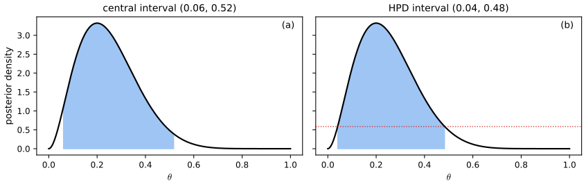
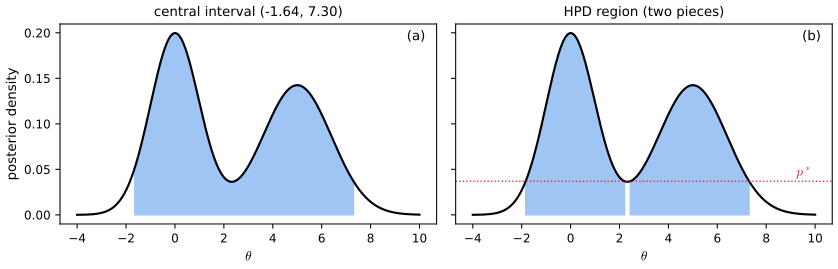
pp. 145–147 A \(100(1-\alpha)\%\) credible interval is a region \(C=(\ell,u)\) with \(P(\ell\le\theta\le u\given\mathcal D)=1-\alpha\) (4.192). The central interval puts \(\alpha/2\) in each tail: \(\ell=F^{-1}(\alpha/2)\), \(u=F^{-1}(1-\alpha/2)\), where \(F\) is the posterior cdf; for a Gaussian this is \(\mu\pm1.96\sigma\). If \(F^{-1}\) is unavailable, use Monte Carlo quantiles of posterior samples. A central interval can contain points of lower density than points outside it; the highest posterior density (HPD) region is \(\{\theta:p(\theta\given\mathcal D)\ge p^*\}\) with \(p^*\) chosen so that the mass is \(1-\alpha\) (4.193)–(4.194). It is the narrowest region of that mass; for a unimodal density it is an interval (the highest density interval, HDI), for a multimodal one it can be several intervals.
Filling the gap 4.14: the HPD region is the smallest-volume region, and has equal density at its ends p. 147
Proof
Optimality ("water-filling"). Let \(C^*=\{p\ge p^*\}\) with \(P(C^*)=1-\alpha\), and \(C\) any measurable set with \(P(C)\ge1-\alpha\). Then \(P(C^*\setminus C)=P(C^*)-P(C^*\cap C)\le P(C)-P(C^*\cap C)=P(C\setminus C^*)\). On \(C^*\setminus C\) the density is \(\ge p^*\) and on \(C\setminus C^*\) it is \(<p^*\), so \(p^*|C^*\setminus C|\le P(C^*\setminus C)\le P(C\setminus C^*)\le p^*|C\setminus C^*|\) (with strict inequality unless the sets differ by a null set), i.e. \(|C^*|\le|C|\). Lowering the level \(p^*\) from the top until 95% of the mass is revealed is the "reverse water-filling" of the book.
Unimodal case. If \(p\) is continuous and unimodal, \(\{p\ge p^*\}=[\ell,u]\) with \(p(\ell)=p(u)=p^*\). Among intervals \([\ell,u]\) of fixed mass, minimise the width \(u-\ell\) with \(F(u)-F(\ell)=1-\alpha\). The Lagrangian condition gives \(1=\mu\,p(u)\) and \(-1=-\mu\,p(\ell)\), hence \(p(\ell)=p(u)\), the equal-density condition (checked numerically for the Beta(3,9) example). This yields the algorithm of the book: scan the lower-tail probability \(q\in[0,\alpha]\), set \(\ell=F^{-1}(q)\), \(u=F^{-1}(q+1-\alpha)\) and keep the narrowest.
Not invariant. The HPD region is not invariant to reparametrisation (the density changes by a Jacobian), whereas the central interval is invariant under monotone transformations.
4.6.7 Bayesian machine learning
pp. 147–151 For conditional models \(p(y\given\bm x,\bm\theta)\) the posterior is over \(\bm\theta\) given \(\mathcal D=\{(\bm x_n,y_n)\}\) and the predictive is (4.195). The plug-in approximation (4.6.7.1) approximates the posterior by a Dirac spike at \(\hat{\bm\theta}\), \(p(\bm\theta\given\mathcal D)=\delta(\bm\theta-\hat{\bm\theta})\) (4.196), giving \(p(y\given\bm x,\mathcal D)\approx p(y\given\bm x,\hat{\bm\theta})\) (4.197) by the sifting property of \(\delta\); it can be over-confident.
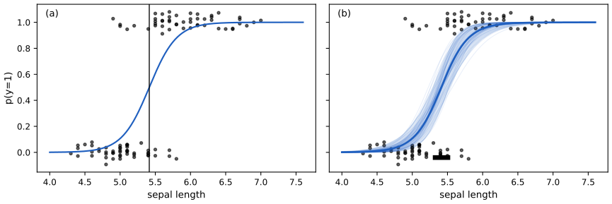
Scalar input, binary output (4.6.7.2). The logistic regression model is \(p(y=1\given x)=\sigma(b+wx)\) (4.198)–(4.201), with \(\sigma(a)=1/(1+e^{-a})\). The decision boundary is the \(x^*\) with \(p(y=1\given x^*)=\tfrac12\), i.e. \(b+wx^*=0\), \(x^*=-b/w\) (4.202)–(4.204). With posterior samples \(\bm\theta_s=(b_s,w_s)\), the predictive is the Monte Carlo average \(p(y=1\given x,\mathcal D)\approx\frac1S\sum_sp(y=1\given x,\bm\theta_s)\) (4.205), and the boundary has a distribution \(p(x^*\given\mathcal D)\approx\frac1S\sum_s\delta(x^*+b_s/w_s)\) (4.206).
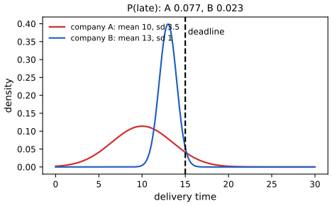
Binary input, scalar output (4.6.7.3). For delivery times with \(p(y\given x,\bm\theta)=\mathcal N(y\given\mu_x,\sigma_x^2)\) (4.207), two data points (one per company) give \(\hat\sigma_0=\hat\sigma_1=0\) by MLE, so the plug-in forecast has no uncertainty; the Bayesian predictive keeps it. Uncertainty matters for decisions: Figure 4.21 shows a company with the smaller mean but larger spread can have the higher probability of missing a deadline (decision theory is the subject of Chapter 5).
Scaling up (4.6.7.4): realistic models have many parameters and the posterior and predictive must be approximated (next section).
4.6.8 Computational issues
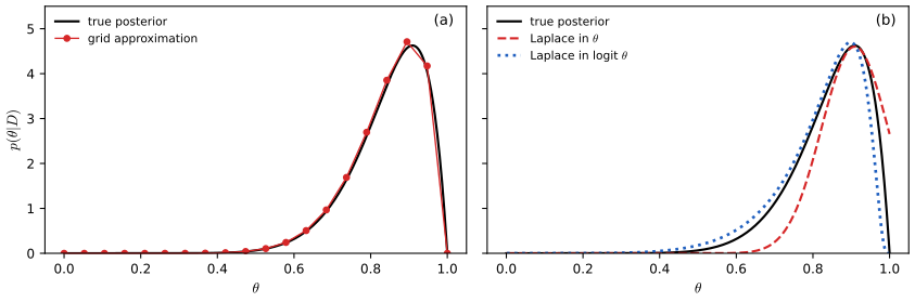
pp. 151–154 Running example: the posterior (4.209) of a beta-Bernoulli model with 10 heads and 1 tail and a uniform prior, exactly \(\operatorname{Beta}(11,2)\), which is highly skewed.
Grid approximation (4.6.8.1): evaluate on points \(\theta_1,\dots,\theta_K\) and normalise, \(p(\theta_k\given\mathcal D)\approx\frac{p(\mathcal D\given\theta_k)p(\theta_k)}{\sum_{k'}p(\mathcal D,\theta_{k'})}\) (4.210). It handles skewness but needs \(K^D\) points in \(D\) dimensions.
Quadratic (Laplace) approximation (4.6.8.2): write \(p(\bm\theta\given\mathcal D)=Z^{-1}e^{-E(\bm\theta)}\) with energy \(E=-\log p(\bm\theta,\mathcal D)\) (4.211) and expand around the mode \(\hat{\bm\theta}\): \(E(\bm\theta)\approx E(\hat{\bm\theta})+\frac12(\bm\theta-\hat{\bm\theta})^\T\bm H(\bm\theta-\hat{\bm\theta})\) (4.212) (the gradient vanishes at the mode). Then \[ \hat p(\bm\theta\given\mathcal D)=\mathcal N(\bm\theta\given\hat{\bm\theta},\bm H^{-1}),\qquad Z\approx e^{-E(\hat{\bm\theta})}(2\pi)^{D/2}|\bm H|^{-1/2}. \tag{4.213--4.215} \]
Filling the gap 4.15: the Laplace approximation for the beta posterior, and why the logit transform helps pp. 152–153
Derivation
For \(\operatorname{Beta}(a,b)\) with \(a=11,b=2\): \(E(\theta)=-(a-1)\log\theta-(b-1)\log(1-\theta)+\mathrm{const}\), mode \(\hat\theta=\frac{a-1}{a+b-2}=\frac{10}{11}\), Hessian \(H=\frac{a-1}{\hat\theta^2}+\frac{b-1}{(1-\hat\theta)^2}=\frac{(a+b-2)^3}{(a-1)(b-1)}=\frac{1331}{10}\), so the Laplace posterior is \(\mathcal N(0.909,0.0075)\), standard deviation \(0.087\): symmetric and with mass above \(\theta=1\), unlike the skewed posterior on \([0,1]\) (Figure 4.22b). In the variable \(\eta=\operatorname{logit}\theta\), \(p(\eta)\propto\theta^{a}(1-\theta)^{b}\) (the Jacobian \(\theta(1-\theta)\) adds one to each exponent), \(\hat\eta=\log(a/b)\), \(H_\eta=(a+b)\bar\theta(1-\bar\theta)\) with \(\bar\theta=a/(a+b)\); the Gaussian in \(\eta\) is mapped back to \(\theta\in(0,1)\) with the Jacobian \(1/(\theta(1-\theta))\), which is skewed in the right direction (Figure 4.22b, dotted). The Laplace formula for the evidence, \(Z\approx e^{-E(\hat{\bm\theta})}(2\pi)^{D/2}|H|^{-1/2}\), is exact for a Gaussian posterior and has relative error \(O(1/N)\) for regular models; it is the basis of the BIC.
Why (4.213) is a normalisation. \(\int\exp\{-\tfrac12(\bm\theta-\hat{\bm\theta})^\T\bm H(\bm\theta-\hat{\bm\theta})\}d\bm\theta=(2\pi)^{D/2}|\bm H|^{-1/2}\), the Gaussian integral, which gives (4.215) on multiplying by \(e^{-E(\hat{\bm\theta})}\).
See also (companion): variational inference (Section 4.6.8.3 of the book: choose \(q\in\mathcal Q\) minimising \(D(q,p)\), leading to the ELBO) and sampling methods (Section 4.6.8.4: MCMC and HMC; the logistic regression figure above uses the simplest, a random-walk Metropolis sampler). These are developed in the sequel to the book; the companion course covers them in its Chapters 10 and 11.
4.7 Frequentist statistics
pp. 154–164 Frequentist statistics avoids priors: the parameter \(\bm\theta^*\) is a fixed unknown constant and the data are random. Uncertainty is the variation of an estimate over repeated data sets.
4.7.1 Sampling distributions
pp. 154–155 An estimator is a function \(\hat\Theta:\mathcal D\mapsto\hat{\bm\theta}\) (the book distinguishes the function \(\hat\Theta\) from its value \(\hat{\bm\theta}=\hat\Theta(\mathcal D)\)). Drawing \(S\) data sets \(\mathcal D^{(s)}\sim\bm\theta^*\) of size \(N\) (4.217) and applying \(\hat\Theta\) to each gives, as \(S\to\infty\), the sampling distribution of the estimator, the push-forward of the data distribution through \(\hat\Theta\) (4.218).
4.7.2 Gaussian approximation of the sampling distribution of the MLE
p. 155 The Fisher information matrix is the covariance of the score, \[ \bm F(\bm\theta)\triangleq\E_{x\sim p(x\given\bm\theta)}\big[\nabla\log p(x\given\bm\theta)\,\nabla\log p(x\given\bm\theta)^\T\big]. \tag{4.220} \]
Result 4.4 (Theorems 4.7.1 and 4.7.2: Fisher information and asymptotic normality) p. 155, (4.219)–(4.222)
Under the regularity conditions (the support does not depend on \(\bm\theta\), differentiation under the integral sign is allowed, the parameter is identifiable and in the interior of the parameter space, and \(\bm F(\bm\theta^*)\succ0\)): (a) the score has mean zero and \(\bm F(\bm\theta)=-\E[\nabla^2\log p(x\given\bm\theta)]\) (4.222). (b) The MLE is consistent and \(\sqrt N(\hat{\bm\theta}_{\rm mle}-\bm\theta^*)\xrightarrow{d}\mathcal N(\bm0,\bm F(\bm\theta^*)^{-1})\), i.e. \(\hat{\bm\theta}\approx\mathcal N(\bm\theta^*,(N\bm F(\bm\theta^*))^{-1})\) (4.219). (c) (Cramér–Rao) any unbiased estimator has \(\operatorname{var}[\hat\theta]\ge1/(NF(\theta^*))\) in the scalar case, so the MLE is asymptotically efficient.
Proof (scalar parameter; the vector case is the same with matrices)
(a) \(\int p(x\given\theta)dx=1\); differentiating, \(0=\int\partial_\theta p\,dx=\int(\partial_\theta\log p)\,p\,dx=\E[s]\), \(s=\partial_\theta\log p\). Differentiating again, \(0=\int(\partial_\theta^2\log p)p\,dx+\int(\partial_\theta\log p)\partial_\theta p\,dx=\E[\partial^2_\theta\log p]+\E[s^2]\). Hence \(F=\E[s^2]=\operatorname{var}[s]=-\E[\partial^2_\theta\log p]\).
(c) Let \(T=\hat\theta(x_{1:N})\) be unbiased, \(\E T=\theta\), and \(S=\sum_n s(x_n)\), the score of the sample, with \(\E S=0\), \(\operatorname{var}S=NF\). Differentiating \(\E T=\theta\) under the integral gives \(1=\int T\partial_\theta\prod p\,dx=\E[TS]=\operatorname{cov}(T,S)\). By Cauchy–Schwarz \(1=\operatorname{cov}(T,S)^2\le\operatorname{var}T\cdot\operatorname{var}S=\operatorname{var}T\cdot NF\), so \(\operatorname{var}T\ge1/(NF)\), with equality iff \(T-\theta\) is proportional to \(S\) almost surely.
(b) (Sketch with the standard assumptions.) The score equation is \(\sum_ns(x_n;\hat\theta)=0\). By the mean value theorem, \(0=\sum_ns(x_n;\theta^*)+(\hat\theta-\theta^*)\sum_n\partial_\theta s(x_n;\tilde\theta)\) for some \(\tilde\theta\) between \(\hat\theta\) and \(\theta^*\), so \[ \sqrt N(\hat\theta-\theta^*)=\frac{N^{-1/2}\sum_ns(x_n;\theta^*)}{-N^{-1}\sum_n\partial_\theta s(x_n;\tilde\theta)}. \] The numerator converges in distribution to \(\mathcal N(0,F)\) by the central limit theorem, since the scores are iid with mean 0 and variance \(F\) (part a). The denominator converges in probability to \(-\E[\partial_\theta s(x;\theta^*)]=F\) by the law of large numbers, consistency (\(\tilde\theta\to\theta^*\)) and continuity. Slutsky's lemma gives \(\mathcal N(0,F/F^2)=\mathcal N(0,1/F)\). Consistency itself follows from the law of large numbers applied to \(N^{-1}\log\text{-likelihood}\to\E\log p(x\given\theta)\), maximised uniquely at \(\theta^*\) by Gibbs' inequality (identifiability); the full argument, including the uniformity needed, is in the companion All of Statistics, Section 9.13.1. \(\square\)
Large curvature of the log-likelihood (large \(F\)) means the parameter is "well determined" and the estimate varies little between data sets. The empirical Fisher, with the expectation replaced by the observed value, is the Hessian of the NLL. The square root of the variance of an estimator is its standard error, estimated in practice by plugging in \(\hat\theta\): for \(X_n\sim\operatorname{Ber}(\theta^*)\) and \(\hat\theta=\bar X\), \(\operatorname{se}=\sqrt{\theta^*(1-\theta^*)/N}\) and \(\widehat{\operatorname{se}}=\sqrt{\hat\theta(1-\hat\theta)/N}\). Here \(F(\theta)=1/(\theta(1-\theta))\), so \(1/(NF)\) is the exact variance and the bound is attained.
See also (companion): All of Statistics, 9.7 asymptotic normality and 9.8 optimality (with the delta method).
4.7.3 Bootstrap approximation of the sampling distribution of any estimator
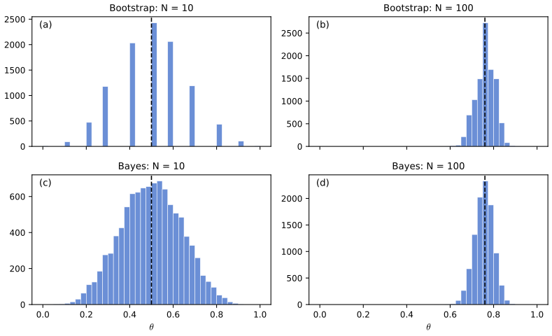
pp. 156–157 If we knew \(\bm\theta^*\) we could simulate data sets \(\tilde{\mathcal D}^{(s)}\sim p(\cdot\given\bm\theta^*)\); since we do not, we sample \(N\) points with replacement from the observed data (the non-parametric bootstrap), apply the estimator to each resample and use the empirical distribution of \(\hat\theta_s=\hat\Theta(\tilde{\mathcal D}^{(s)})\). (The parametric bootstrap samples from \(p(\cdot\given\hat{\bm\theta})\).) For the Bernoulli MLE the sampling distribution is skewed for \(N=10\) and nearly Gaussian for \(N=100\) (Figure 4.23, top). A bootstrap sample contains on average \(0.632N\) distinct observations.
Filling the gap 4.16: the 0.632 fraction, and why the bootstrap works p. 157
Derivation
Fix an observation. In one draw it is missed with probability \(1-1/N\), so it is missed in all \(N\) draws with probability \((1-1/N)^N\to e^{-1}\) (since \(\log(1-1/N)^N=N\log(1-1/N)=-1-\frac1{2N}-\dots\to-1\)). It appears at least once with probability \(1-(1-1/N)^N\to1-e^{-1}\approx0.632\), and by linearity of expectation the expected number of distinct observations is \(N[1-(1-1/N)^N]\approx0.632N\) (the code confirms 0.632 for \(N=1000\)).
Why it works. Bootstrap resampling draws iid samples from the empirical distribution \(\hat P_N\), which converges to the true distribution \(P\) (Glivenko–Cantelli). For a smooth functional \(T\) the sampling distribution of \(\hat\Theta(\tilde{\mathcal D})\) under \(\hat P_N\) therefore approximates that under \(P\): the "bootstrap world" mimics the real world. For the Bernoulli mean the bootstrap distribution of \(\hat\theta^*=\frac1N\operatorname{Bin}(N,\hat\theta)\) is exactly known: its variance is \(\hat\theta(1-\hat\theta)/N\), the plug-in standard error of Section 4.7.2 (the demo checks this by simulation).
Section 4.7.3.1 of the book remarks that the bootstrap can be slower than posterior sampling because it refits the model \(S\) times; in return it needs no prior and no likelihood beyond the estimator. See also All of Statistics, 8.3 and the bootstrap replicates demo.
4.7.4 Confidence intervals
pp. 157–158 A \(100(1-\alpha)\%\) confidence interval is a data-dependent interval \(I(\mathcal D)=(\ell(\mathcal D),u(\mathcal D))\) with \(\Pr\big(\theta^*\in I(\tilde{\mathcal D})\mid\tilde{\mathcal D}\sim\theta^*\big)\ge1-\alpha\) (4.223): in repeated sampling at least \(100(1-\alpha)\%\) of such intervals contain \(\theta^*\). If the law of \(\Delta=\theta^*-\hat\theta\) were known with quantiles \(\underline\delta,\overline\delta\) at \(\alpha/2\) and \(1-\alpha/2\) then \(\Pr(\hat\theta+\underline\delta\le\theta^*\le\hat\theta+\overline\delta)=1-\alpha\) (4.224–4.225) and \(I=(\hat\theta+\underline\delta,\hat\theta+\overline\delta)\) (4.226). With the Gaussian approximation \(\hat\theta\approx\mathcal N(\theta^*,\widehat{\operatorname{se}}^2)\), \[ I=(\hat\theta-z_{\alpha/2}\widehat{\operatorname{se}},\ \hat\theta+z_{\alpha/2}\widehat{\operatorname{se}}),\qquad z_{0.025}=1.96, \tag{4.227} \] i.e. \(\hat\theta\pm2\widehat{\operatorname{se}}\) (a Wald interval). Otherwise use the bootstrap distribution of \(\hat\theta-\hat\theta^{(s)}\) as a stand-in for that of \(\Delta\).
Filling the gap 4.17: the bootstrap confidence interval (the "pivotal" interval) p. 158
Derivation
Let \(\hat\theta^*_s\) be the estimate on bootstrap sample \(s\), with the empirical \(\alpha/2\) and \(1-\alpha/2\) quantiles \(q_{\alpha/2},q_{1-\alpha/2}\) of \(\hat\theta^*_s\). The bootstrap analogue of \(\Delta=\theta^*-\hat\theta\) is \(\hat\theta-\hat\theta^*_s\) (the "true" parameter of the bootstrap world is \(\hat\theta\)). Its quantiles are \(\hat\theta-q_{1-\alpha/2}\) and \(\hat\theta-q_{\alpha/2}\). Inserting into (4.226), \(I=\big(2\hat\theta-q_{1-\alpha/2},\ 2\hat\theta-q_{\alpha/2}\big)\), the basic (pivotal) bootstrap interval, which reflects the quantiles of \(\hat\theta^*\) about \(\hat\theta\) and differs from the percentile interval \((q_{\alpha/2},q_{1-\alpha/2})\) when the bootstrap distribution is skewed. Both are first-order accurate; the justification is in All of Statistics, Section 8.5.2.
4.7.5 Caution: confidence intervals are not credible
pp. 158–159 A 95% confidence interval does not say \(p(\theta^*\in I\given\mathcal D)=0.95\). That quantity belongs to a Bayesian credible interval. The confidence statement concerns the procedure over hypothetical repetitions, with \(\theta\) fixed and the data random; the credible statement conditions on the one data set seen, with \(\theta\) random. Bayes: \(\Pr(\theta^*\in I)=0.95\) over data sets can coexist with certainty, for some data sets, that \(\theta^*\in I\) or \(\notin I\).
Filling the gap 4.18: the two-integer example and the Wald interval's failures pp. 158–159, (4.228)–(4.231)
Derivation
Berger's example. Two integers \(y_1,y_2\) are drawn independently, each equal to \(\theta\) or \(\theta+1\) with probability \(\frac12\). With \(m=\min(y_1,y_2)\) and the degenerate interval \([m,m]\): \(m=\theta\) unless both equal \(\theta+1\) (probability \(\frac14\)), so the coverage is exactly \(\frac34\) for every \(\theta\): a valid 75% confidence interval. But if \(y_1\ne y_2\), then \(\{y_1,y_2\}=\{\theta,\theta+1\}\), hence \(\theta=\min(y_1,y_2)\) with certainty, while the interval still claims only 75% confidence. With a flat prior on the integers, the posterior puts probability 1 on \(\theta=m\) when \(y_1\ne y_2\), and probability \(\tfrac12\) on each of \(\theta=m-1\) and \(\theta=m\) when \(y_1=y_2=m\): conditional on the data, the correct statements are 1 or 1/2, never 0.75. The coverage is an average over data sets, and for the particular data set one has it can be the wrong summary.
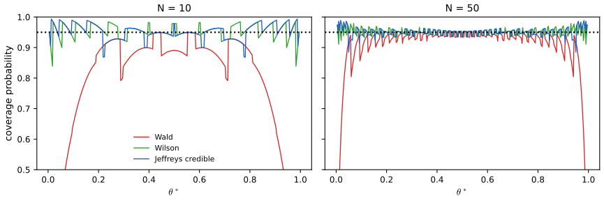
The Wald interval for a Bernoulli parameter. For \(N=1,y_1=0\): \(\hat\theta=0\) and \(\bar y\pm1.96\sqrt{\bar y(1-\bar y)/N}=(0,0)\): a zero-width interval, which can never contain \(\theta^*\in(0,1)\). More generally the coverage of the Wald interval at \(\theta\) is \(c(\theta)=\sum_k\binom Nk\theta^k(1-\theta)^{N-k}\mathbb I(\theta\in I_k)\), exactly computable; it oscillates in \(\theta\) with downward spikes near 0 and 1 even for large \(N\) (Brown, Cai and DasGupta, 2001). The Wilson interval (the set of \(\theta\) with \(|\hat\theta-\theta|\le1.96\sqrt{\theta(1-\theta)/N}\), obtained by solving a quadratic) and the Jeffreys credible interval (the central interval of the \(\operatorname{Beta}(k+\frac12,N-k+\frac12)\) posterior) have coverage close to 95% across the range (supplementary Figure 4.S1). So a Bayesian interval, built to condition on the data, here also behaves well as a confidence procedure.
See also: credible interval coverage and confidence interval coverage demos in the All of Statistics course.
4.7.6 The bias-variance tradeoff
4.7.6.1 Bias of an estimator
pp. 159–160 \(\operatorname{bias}(\hat\theta)\triangleq\E[\hat\theta(\mathcal D)]-\theta^*\) (4.232), expectation over \(p(\mathcal D\given\theta^*)\). The sample mean is unbiased (4.233); the MLE of the Gaussian variance satisfies \(\E[\hat\sigma^2_{\rm mle}]=\frac{N-1}N\sigma^2\) (4.234), while \(\hat\sigma^2_{\rm unb}=\frac N{N-1}\hat\sigma^2_{\rm mle}\) (4.235) is unbiased (4.236). If \(\mu\) is known, the MLE of \(\sigma^2\) is unbiased (Exercise 4.8). Proofs are in Exercises 4.7 and 4.8 below.
4.7.6.2 Variance of an estimator
p. 160 \(\operatorname{var}[\hat\theta]=\E[\hat\theta^2]-(\E\hat\theta)^2\) (4.237). Unbiasedness is not enough: \(\hat\theta=x_1\) is unbiased for a Gaussian mean but has variance \(\sigma^2\) instead of \(\sigma^2/N\). The Cramér–Rao bound (Result 4.4c) gives the smallest variance of an unbiased estimator, attained asymptotically by the MLE.
4.7.6.3 The bias-variance tradeoff
p. 161 With \(\bar\theta=\E\hat\theta\), \[ \E[(\hat\theta-\theta^*)^2]=\operatorname{var}[\hat\theta]+\operatorname{bias}^2(\hat\theta), \tag{4.238--4.242} \] since \(\E[(\hat\theta-\bar\theta)+(\bar\theta-\theta^*)]^2\) has a vanishing cross term \(2(\bar\theta-\theta^*)\E[\hat\theta-\bar\theta]=0\) (the book's (4.238) puts the square outside the expectation; the meaning is as above). A biased estimator can have a smaller MSE if it reduces variance by more than the squared bias.
4.7.6.4 Example: MAP estimator for a Gaussian mean
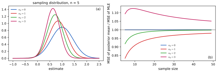
pp. 161–162 Data \(x_n\sim\mathcal N(\theta^*,\sigma^2)\). The MLE \(\bar x\) has bias 0 and variance \(\sigma^2/N\) (4.243). The posterior mean (equal to the MAP) under a \(\mathcal N(\theta_0,\sigma^2/\kappa_0)\) prior is \(\tilde x=w\bar x+(1-w)\theta_0\), \(w=\frac N{N+\kappa_0}\) (4.244), with bias \((1-w)(\theta_0-\theta^*)\) and variance \(w^2\sigma^2/N\) (4.245–4.246).
Filling the gap 4.19: when does shrinkage beat the MLE? (Figure 4.24) pp. 161–162
Derivation
\(\operatorname{MSE}(\tilde x)=w^2\frac{\sigma^2}N+(1-w)^2\delta^2\) with \(\delta=\theta_0-\theta^*\), against \(\sigma^2/N\) for the MLE. Using \(1-w=\kappa_0/(N+\kappa_0)\), \(1+w=(2N+\kappa_0)/(N+\kappa_0)\): \(\operatorname{MSE}(\tilde x)<\operatorname{MSE}(\bar x)\iff(1-w)^2\delta^2<(1-w^2)\frac{\sigma^2}N\iff(1-w)\delta^2<(1+w)\frac{\sigma^2}N\iff\) \[ \delta^2<\frac{\sigma^2}{N}\Big(\frac{2N}{\kappa_0}+1\Big). \] The condition holds for all \(N\) whenever the prior mean is within \(\sigma\sqrt{2/\kappa_0}\) of the truth, and for small \(N\) it tolerates a much larger prior error. With \(\theta^*=1,\theta_0=0,\sigma=1\) (\(\delta=1\)): at \(n=5\), \(\kappa_0=1\): right side \(2.2>1\); \(\kappa_0=2\): \(1.2>1\), shrinkage wins; \(\kappa_0=3\): \(13/15<1\), it loses, as in Figure 4.24b. A prior that is too strong when it is wrong costs more than the variance it saves; \(\kappa_0\to0\) gives back the MLE. As \(N\to\infty\) the right side tends to \(\sigma^2/N\cdot(2N/\kappa_0)=2\sigma^2/\kappa_0\), still positive, so a mild prior always helps if \(\delta^2<2\sigma^2/\kappa_0\).
4.7.6.5 Example: MAP estimator for linear regression
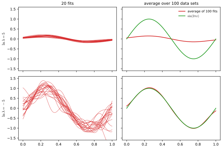
pp. 162–163 Ridge regression is MAP with \(p(\bm w)=\mathcal N(0,\lambda^{-1}\bm I)\). Increasing \(\lambda\) lowers the variance of the fitted curve and raises its bias (Figure 4.25: 100 data sets, a Gaussian-bump basis with 25 centres on \([0,1]\), the truth \(\sin2\pi x\)).
Filling the gap 4.20: the bias and variance of the ridge fit in closed form p. 162
Derivation
With fixed design \(\bm\Phi\) and \(\bm y=\bm f+\bm\varepsilon\), \(\operatorname{cov}\bm\varepsilon=\sigma^2\bm I\), the ridge fit at the training inputs is \(\hat{\bm f}=\bm S_\lambda\bm y\), \(\bm S_\lambda=\bm\Phi(\bm\Phi^\T\bm\Phi+\lambda\bm I)^{-1}\bm\Phi^\T\). Then \(\E\hat{\bm f}=\bm S_\lambda\bm f\), bias \(=(\bm S_\lambda-\bm I)\bm f\), covariance \(\sigma^2\bm S_\lambda\bm S_\lambda^\T\). In the SVD basis \(\bm\Phi=\bm U\bm D\bm V^\T\), \(\bm S_\lambda=\bm U\operatorname{diag}\big(\frac{d_i^2}{d_i^2+\lambda}\big)\bm U^\T\), so the total variance is \(\sigma^2\sum_i\big(\frac{d_i^2}{d_i^2+\lambda}\big)^2\), decreasing in \(\lambda\) and equal to \(\sigma^2\operatorname{rank}\) at \(\lambda=0\), and the squared bias is \(\sum_i\big(\frac\lambda{d_i^2+\lambda}\big)^2(\bm u_i^\T\bm f)^2+\|\bm f-\bm P\bm f\|^2\), increasing in \(\lambda\) (with \(\bm P\) the projection onto the column space). Their sum is the MSE; the best \(\lambda\) balances the two. Figure 4.25 shows the same trade-off for the whole fitted function.
See also (companion): bias–variance demo and Section 3.2. Figure 4.26 of the book is a hand-drawn cartoon of error against model complexity and is not reproduced.
4.7.6.6 Bias-variance tradeoff for classification
p. 164 For 0-1 loss the risk is no longer squared bias plus variance; the two combine multiplicatively (Friedman, 1997; Hastie, Tibshirani and Friedman, Exercise 7.2). If the average estimate is on the correct side of the decision boundary, the bias is "negative" and reducing the variance reduces the error rate; if it is on the wrong side, the bias is "positive" and increasing the variance helps. The practical advice is to estimate the expected loss directly, by cross-validation (Section 4.5.5), rather than reason through bias and variance.
4.8 Exercises
All nine exercises of Chapter 4 (Murphy, 2022, pp. 164–166), restated in my own words, with complete solutions (hidden). Dagger marks the book's own flag for solutions available in its solution material; here every solution is worked independently.
Exercise 4.1. Show that the MLE of a univariate Gaussian is \(\hat\mu=\bar y\), \(\hat\sigma^2=\frac1N\sum_n(y_n-\hat\mu)^2\) (4.247)–(4.248).
Solution
This is Filling the gap 4.2: set the two partial derivatives of (4.33) to zero, obtain \(\mu=\bar y\) and \(\sigma^2=\frac1N\sum(y_n-\bar y)^2\), and check that the stationary point is the global minimum by the profile argument given there. \(\square\)
Exercise 4.2. Samples \(x_1,\dots,x_n\sim\mathcal N(\mu,\sigma^2)\) with \(\sigma^2\) known and prior \(\mu\sim\mathcal N(m,s^2)\). (a) Find \(\hat\mu_{\rm MAP}\). (b) Show that it converges to the MLE as \(n\to\infty\). (c) What is the limit as \(s^2\to\infty\) for fixed small \(n\)? (d) And as \(s^2\to0\)?
Solution
(a) The log posterior is \(-\frac1{2\sigma^2}\sum(x_i-\mu)^2-\frac1{2s^2}(\mu-m)^2+\mathrm{const}\), a concave quadratic; setting its derivative to zero, \(\frac n{\sigma^2}(\bar x-\mu)-\frac1{s^2}(\mu-m)=0\), so \[ \hat\mu_{\rm MAP}=\frac{\frac n{\sigma^2}\bar x+\frac1{s^2}m}{\frac n{\sigma^2}+\frac1{s^2}}=\frac{ns^2\bar x+\sigma^2m}{ns^2+\sigma^2}. \] (b) The weight on the prior mean is \(\sigma^2/(ns^2+\sigma^2)\to0\) as \(n\to\infty\), so \(\hat\mu_{\rm MAP}-\bar x=\frac{\sigma^2}{ns^2+\sigma^2}(m-\bar x)\to0\) (and \(\bar x\) is the MLE). (c) As \(s^2\to\infty\) the weight on \(m\) tends to 0 and \(\hat\mu_{\rm MAP}\to\bar x=\hat\mu_{\rm MLE}\): a flat prior. (d) As \(s^2\to0\) the weight on \(m\) tends to 1 and \(\hat\mu_{\rm MAP}\to m\): the data are ignored. \(\square\)
Exercise 4.3. Let \(X\sim\mathcal N(\mu,\sigma^2=4)\) with \(\mu\sim\mathcal N(\mu_0,\sigma_0^2=9)\). After \(n\) samples the posterior is \(\mathcal N(\mu_n,\sigma_n^2)\). How large must \(n\) be so that an interval of width 1 centred on \(\mu_n\) has posterior probability at least 0.95?
Solution
By (4.173), \(1/\sigma_n^2=n/4+1/9\), independent of the data. An interval \(\mu_n\pm\frac12\) has posterior mass at least 0.95 iff \(\frac12\ge1.96\sigma_n\), i.e. \(\sigma_n^2\le(0.5/1.96)^2=0.06507\), i.e. \(n/4+1/9\ge15.366\), \(n\ge4(15.366-0.111)=61.02\). So \(n\ge62\) (checked numerically: \(n=61\) gives interval mass \(0.94996\), just short, and \(n=62\) gives \(0.9518\)). \(\square\)
Exercise 4.4. Using \(\mathrm{BIC}=\log p(\mathcal D\given\hat{\bm\theta}_{\rm ML})-\frac d2\log N\) (4.250) and \(\log p(\mathcal D\given\hat\Sigma,\hat\mu)=-\frac N2\operatorname{tr}(\hat\Sigma^{-1}\hat S)-\frac N2\log|\hat\Sigma|\) (4.251) (up to the constant \(-\frac{ND}2\log2\pi\)), derive the BIC for a \(D\)-dimensional Gaussian with (a) a full covariance matrix and (b) a diagonal one.
Solution
(a) The MLE is \(\hat\Sigma=\hat S\), so \(\operatorname{tr}(\hat\Sigma^{-1}\hat S)=\operatorname{tr}\bm I_D=D\). The number of free parameters is \(d=D\) (mean) \(+D(D+1)/2\) (symmetric covariance) \(=D(D+3)/2\). Hence \[ \mathrm{BIC}_{\rm full}=-\frac N2\log|\hat S|-\frac{ND}2-\frac{D(D+3)}4\log N. \] (b) With a diagonal covariance the MLE is \(\hat\Sigma_{\rm diag}=\operatorname{diag}(\hat S_{11},\dots,\hat S_{DD})\), so \(\operatorname{tr}(\hat\Sigma_{\rm diag}^{-1}\hat S)=\sum_i\hat S_{ii}/\hat S_{ii}=D\), \(\log|\hat\Sigma_{\rm diag}|=\sum_i\log\hat S_{ii}\) and \(d=2D\): \[ \mathrm{BIC}_{\rm diag}=-\frac N2\sum_i\log\hat S_{ii}-\frac{ND}2-D\log N. \] The difference \(\mathrm{BIC}_{\rm full}-\mathrm{BIC}_{\rm diag}=\frac N2\big(\sum_i\log\hat S_{ii}-\log|\hat S|\big)-\frac{D(D-1)}4\log N\); by Hadamard's inequality \(\log|\hat S|\le\sum\log\hat S_{ii}\), so the first term is the non-negative gain in fit from modelling correlations, and the second is the penalty for the extra \(D(D-1)/2\) parameters. (Constants \(-\frac{ND}2\log2\pi\) cancel in the comparison.) \(\square\)
Exercise 4.5. A coin has heads probability \(\theta_1\); a friend reports the outcome \(y\), correctly with probability \(\theta_2\) independent of everything else. (a) Write the joint \(p(x,y\given\bm\theta)\) as a table. (b) Data \(\bm x=(1,1,0,1,1,0,0)\), \(\bm y=(1,0,0,0,1,0,1)\): find the MLEs and \(p(\mathcal D\given\hat{\bm\theta},\mathcal M_2)\). (c) For the model with four free cell probabilities \(\theta_{x,y}\) find the MLE and \(p(\mathcal D\given\hat{\bm\theta},\mathcal M_4)\). (d) Which model does leave-one-out cross-validation of the log-likelihood pick? (e) Which does BIC pick?
Solution
(a) \(p(x,y)=p(x\given\theta_1)p(y\given x,\theta_2)\): rows \(x=0\): \((1-\theta_1)\theta_2\) for \(y=0\) and \((1-\theta_1)(1-\theta_2)\) for \(y=1\); row \(x=1\): \(\theta_1(1-\theta_2)\) for \(y=0\) and \(\theta_1\theta_2\) for \(y=1\).
(b) The likelihood factorises, \(p(\mathcal D)=\big[\theta_1^{4}(1-\theta_1)^3\big]\big[\theta_2^{a}(1-\theta_2)^{7-a}\big]\) with \(a\) the number of agreements. \(\sum x=4\) gives \(\hat\theta_1=4/7\). The pairs \((x,y)\) are \((1,1),(1,0),(0,0),(1,0),(1,1),(0,0),(0,1)\): the agreements are positions 1, 3, 5, 6, so \(a=4\) and \(\hat\theta_2=4/7\). Then \(p(\mathcal D\given\hat{\bm\theta},\mathcal M_2)=(4/7)^4(3/7)^3\cdot(4/7)^4(3/7)^3=(4/7)^8(3/7)^6\approx7.1\times10^{-5}\), \(\log=-9.5607\).
(c) The counts of \((x,y)=(0,0),(0,1),(1,0),(1,1)\) are \(2,1,2,2\), so \(\hat\theta_{x,y}=n_{xy}/7\) and \(p(\mathcal D\given\hat{\bm\theta},\mathcal M_4)=(2/7)^6(1/7)\), \(\log=-9.4625\): slightly larger than for \(\mathcal M_2\) (it has more freedom, and \(\mathcal M_2\subset\mathcal M_4\)).
(d) Under \(\mathcal M_4\), leaving out the only observation with \((x,y)=(0,1)\) leaves \(\hat\theta_{01}=0\), so the held-out point has probability 0 and log-probability \(-\infty\); the LOO score of \(\mathcal M_4\) is \(-\infty\). Under \(\mathcal M_2\) every held-out probability is positive (\(\hat\theta_1\) and \(\hat\theta_2\) stay strictly inside \((0,1)\)), so its score is finite. LOO picks \(\mathcal M_2\).
(e) \(\mathrm{BIC}(\mathcal M_2)=-9.5607-\frac22\log7=-11.507\); \(\mathrm{BIC}(\mathcal M_4)=-9.4625-\frac32\log7=-12.381\) (3 free parameters). BIC also prefers \(\mathcal M_2\). (Computed with the code of this chapter.) \(\square\)
Exercise 4.6. Prove that a mixture of conjugate priors is conjugate.
Solution
See Filling the gap 4.10: the posterior of \(\sum_kw_kp_k(\theta)\) is \(\sum_k\frac{w_km_k}{\sum_jw_jm_j}p_k(\theta\given\mathcal D)\) with \(m_k=\int p(\mathcal D\given\theta)p_k(\theta)d\theta\). \(\square\)
Exercise 4.7. Show that \(\hat\sigma^2_{\rm MLE}=\frac1N\sum_n(x_n-\hat\mu)^2\) is a biased estimator of \(\sigma^2\) for \(x_n\sim\mathcal N(\mu,\sigma^2)\).
Solution
Write \(\sum_n(x_n-\bar x)^2=\sum_nx_n^2-N\bar x^2\). Now \(\E x_n^2=\sigma^2+\mu^2\), and by independence \(\E\bar x^2=\operatorname{var}\bar x+\mu^2=\sigma^2/N+\mu^2\). So \(\E\sum(x_n-\bar x)^2=N(\sigma^2+\mu^2)-N(\sigma^2/N+\mu^2)=(N-1)\sigma^2\) and \(\E\hat\sigma^2_{\rm MLE}=\frac{N-1}N\sigma^2\ne\sigma^2\): the bias is \(-\sigma^2/N\). (Independence is used only in \(\operatorname{var}\bar x=\sigma^2/N\), i.e. \(\E[x_ix_j]=\mu^2\) for \(i\ne j\); the Gaussian assumption is not needed.) \(\square\)
Exercise 4.8. If \(\mu\) is known, derive the MLE of \(\sigma^2\) and say whether it is unbiased.
Solution
\(\operatorname{NLL}(\sigma^2)=\frac1{2\sigma^2}\sum(x_n-\mu)^2+\frac N2\log\sigma^2+\mathrm{const}\), minimised (by the profile argument of Gap 4.2) at \(\hat\sigma^2=\frac1N\sum_n(x_n-\mu)^2\). Since \(\E(x_n-\mu)^2=\sigma^2\), \(\E\hat\sigma^2=\sigma^2\): unbiased. The loss of one degree of freedom in Exercise 4.7 comes from estimating \(\mu\) by \(\bar x\), which makes the residuals fit slightly too well. \(\square\)
Exercise 4.9. Show that the standard error of \(\hat\sigma^2_{\rm mle}\) is \(\sqrt{\operatorname{var}[\hat\sigma^2_{\rm mle}]}=\sqrt{2(N-1)/N^2}\,\sigma^2\) (4.258), using \(\frac{N-1}{\sigma^2}\hat\sigma^2_{\rm unb}\sim\chi^2_{N-1}\) and \(\operatorname{var}\chi^2_{N-1}=2(N-1)\); and compute the MSE of the two estimators.
Solution
\(\operatorname{var}[\hat\sigma^2_{\rm unb}]=\frac{\sigma^4}{(N-1)^2}\cdot2(N-1)=\frac{2\sigma^4}{N-1}\). Since \(\hat\sigma^2_{\rm mle}=\frac{N-1}N\hat\sigma^2_{\rm unb}\), \(\operatorname{var}[\hat\sigma^2_{\rm mle}]=\frac{(N-1)^2}{N^2}\cdot\frac{2\sigma^4}{N-1}=\frac{2(N-1)}{N^2}\sigma^4\), whose square root is (4.258). MSE = variance + bias\(^2\) (4.242). The unbiased estimator has \(\operatorname{MSE}(\hat\sigma^2_{\rm unb})=\frac{2}{N-1}\sigma^4\). The MLE has bias \(-\sigma^2/N\), so \(\operatorname{MSE}(\hat\sigma^2_{\rm mle})=\frac{2(N-1)}{N^2}\sigma^4+\frac{\sigma^4}{N^2}=\frac{2N-1}{N^2}\sigma^4\). The book's statement of the end of the exercise has the two formulas attached to the wrong estimators (see the notes on the book). The biased MLE has the smaller MSE for every \(N\ge2\) because \(\frac{2N-1}{N^2}<\frac2{N-1}\iff(2N-1)(N-1)<2N^2\iff1<3N\). A simulation with \(N=6,\sigma^2=4\) (200,000 data sets) gives MSE \(4.89\) (MLE; formula \(\frac{11}{36}\cdot16=4.89\)) and \(6.40\) (unbiased; formula \(\frac25\cdot16=6.4\)). \(\square\)
Demonstrations
| Page | What it shows | In the notes |
|---|---|---|
| The beta-binomial model | Prior, rescaled likelihood and posterior of a coin's heads probability; credible and HPD intervals; predictive against plug-in; mixture prior. Presets: 1 Beta(2,2); 2 uniform; 3 predictive; 4 mixture; 5 zero counts. | 4.6.2, gap 4.10 |
| Ridge regression and cross-validation | A polynomial fitted to 21 points with a ridge penalty; training, test and K-fold CV errors with the one-SE rule. Presets: 1 overfit; 2 good fit; 3 underfit; 4 one-SE; 5 degree 3. | 4.5.3, 4.5.5, Result 4.3 |
| Bootstrap, posterior and confidence intervals | Bootstrap distribution of the Bernoulli MLE against the posterior; exact coverage of Wald, Wilson and Jeffreys intervals. Presets: 1 N=10; 2 N=100; 3 one toss; 4 rare event; 5 N=100, theta=0.03. | 4.7.3, 4.7.5, gap 4.18 |
The Python code that produces every figure of this page is code/ch04_statistics.py (see the code index). Companion demos: conjugate priors, bias–variance, bootstrap replicates.
Notes on the book
Points where the book is imprecise or wrong
- Figure 4.2 versus (4.66). The text says the log loss \(\log(1+e^{-\tilde y\eta})\) is a smooth upper bound on the 0-1 loss, but with the natural log it is \(\ln2=0.69<1\) at the margin 0; the figure caption uses \(\log_2\), for which the bound holds. The bound needs the base-2 scaling (Result 4.2).
- Section 4.5.5.1. The standard error is described as "the mean of the sampling distribution of the estimate"; it is the standard deviation of that distribution (and the formula \(\hat\sigma/\sqrt N\) is a standard deviation).
- Exercise 4.9. The two MSE formulas are attached to the wrong estimators: \(\operatorname{MSE}(\hat\sigma^2_{\rm unb})=2\sigma^4/(N-1)\) and \(\operatorname{MSE}(\hat\sigma^2_{\rm mle})=(2N-1)\sigma^4/N^2\) (the book states them the other way round). Verified by exact algebra and by simulation (Exercise 4.9).
- (4.97) and "prior sample size". With the usual inverse-Wishart parametrisation the posterior mode is \((\bm\Psi+\bm S_y)/(\nu+D+1+N)\); the book's \(\breve N\) is therefore \(\nu+D+1\), not the degrees of freedom (Filling the gap 4.5).
- Section 4.6.4.1 refers to "Bayes' rule for Gaussians, as in Section 4.6.4.1", which is a self-reference; the relevant material is Section 3.3.1 (and the multivariate version in 4.6.4.2).
- (4.238). The squared sum is written outside the expectation; the intended expression is \(\E[((\hat\theta-\bar\theta)+(\bar\theta-\theta^*))^2]\).
- (4.8). The joint-likelihood MLE is written with \(\argmin\) of the negative sum, correct, but (4.5) and (4.7) switch between \(\argmax\) and \(\argmin\) without comment; read them as the same estimator.
References
- Murphy, K. P. (2022). Probabilistic Machine Learning: An Introduction. MIT Press, Cambridge, MA. Chapter 4, pp. 107–166. probml.github.io/pml-book/book1.html.
- Berger, J. O. (1985). Statistical Decision Theory and Bayesian Analysis, 2nd edition. Springer, New York.
- Bishop, C. M. (2006). Pattern Recognition and Machine Learning. Springer, New York.
- Brown, L. D., Cai, T. T. and DasGupta, A. (2001). Interval estimation for a binomial proportion. Statistical Science, 16(2), 101–133.
- Efron, B. (1979). Bootstrap methods: another look at the jackknife. Annals of Statistics, 7(1), 1–26.
- Fisher, R. A. (1936). The use of multiple measurements in taxonomic problems. Annals of Eugenics, 7(2), 179–188.
- Friedman, J. H. (1997). On bias, variance, 0/1 loss, and the curse of dimensionality. Data Mining and Knowledge Discovery, 1(1), 55–77.
- Hastie, T., Tibshirani, R. and Friedman, J. (2009). The Elements of Statistical Learning, 2nd edition. Springer, New York.
- Hoerl, A. E. and Kennard, R. W. (1970). Ridge regression: biased estimation for nonorthogonal problems. Technometrics, 12(1), 55–67.
- Ledoit, O. and Wolf, M. (2004). A well-conditioned estimator for large-dimensional covariance matrices. Journal of Multivariate Analysis, 88(2), 365–411.
- Rice, J. A. (1995). Mathematical Statistics and Data Analysis, 2nd edition. Duxbury Press, Belmont, CA.
- Wasserman, L. (2004). All of Statistics. Springer, New York.
- Wilson, E. B. (1927). Probable inference, the law of succession, and statistical inference. Journal of the American Statistical Association, 22(158), 209–212.
The numerical statements in the text (maximum likelihood formulas, the method-of-moments example, shrinkage covariance estimates, the leave-one-out shortcut, the mixture-of-betas posterior and the probabilities 0.346, 0.654, 0.9604 and 0.8858, the HPD and central intervals of the Beta(3,9) posterior, Laplace's approximation, the Wald, Wilson and Jeffreys coverage, the bias and MSE formulas and the numerical answers to the exercises) were confirmed numerically.