Message passing algorithms
Message passing turns the conditional independences of a graphical model into dynamic programming: local messages, passed along the edges of a chain, a tree, a loopy graph or a junction tree, give marginals, modes and samples without enumerating the joint. This chapter covers forwards-backwards and Viterbi for HMMs, belief propagation on trees and polytrees, loopy and Gaussian BP with their convergence, decoding and clustering applications, variable elimination and the junction tree, inference as differentiation and as optimisation (perturb-and-MAP), and the MAP problem for discrete models by linear programming and graph cuts.
Ch. 1 Introduction Ch. 2 Probability Ch. 3 Statistics Ch. 4 Graphical models Ch. 5 Information theory Ch. 6 Optimisation Ch. 7 Inference algorithms Ch. 8 Gaussian filtering Ch. 9 Message passing Ch. 10 Variational inference Ch. 11 Monte Carlo Ch. 12 MCMC Ch. 13 Sequential Monte Carlo Ch. 14 Predictive models Ch. 15 GLMs Ch. 16 Deep networks Ch. 17 Bayesian neural networks Ch. 18 Gaussian processes Ch. 19 Beyond iid Ch. 20 Generative models Ch. 21 VAEs Ch. 22 Autoregressive models Ch. 23 Normalizing flows Ch. 24 Energy-based models Ch. 25 Diffusion models Ch. 26 GANs Ch. 27 Discovery methods Ch. 28 Latent factor models Ch. 29 State-space models Ch. 30 Graph learning Ch. 31 Nonparametric Bayes Ch. 32 Representation learning Ch. 33 Interpretability Ch. 34 Decision making Ch. 35 Reinforcement learning Ch. 36 Causality
How to read these notes
They follow the book. Sections carry the book's numbers (9.2, 9.4.4, ...) and displayed equations that appear in the book carry its equation numbers, e.g. \((9.17)\). Material from the online supplement is placed where it belongs and labelled (supplement); its equations are written (S9.k) after the supplement's own numbers, to keep them apart from the main text.
Filling the gaps. Wherever the book states a result without proof, leaves a calculation to the reader or quotes the literature, an orange Filling the gap box (or a proof) gives the argument. Derivations start hidden: open one with its bar, or use the buttons below.
Figures and demonstrations. Every figure of the chapter that is computed from a model or a simulation is reproduced from scratch by the Python code; hand-drawn diagrams are not redrawn. Figures named 9.S1 to 9.S5 are our own, added to illustrate a result. The book's data are simulated, so the samples differ from the book's (the numbers differ accordingly, and we say so).
Main reference
K. P. Murphy, Probabilistic Machine Learning: Advanced Topics, MIT Press (2023; the December 2025 draft is followed), Chapter 9, pages 401–438, and Supplementary Chapter 9, pages 99–122 (book web page: probml.github.io/pml-book/book2.html).
The explanations, derivations, figures and code are my own; equations are cited by their numbers in the book.
Companion courses
This chapter overlaps with finished material on this site, and the proofs there are not repeated here:
- Sum-product and max-sum on trees and factor graphs, the junction tree in outline, with proofs, in Bishop's notation: Bayesian and Probabilistic Machine Learning, Chapter 8; forwards-backwards, scaling and Viterbi for HMMs: Chapter 13.
- The exponential family and its mean parameters (used in 9.7): Chapter 2 of this course; graphical models and factor graphs: Chapter 4; inference overview: Chapter 7; Kalman smoothing, the continuous analogue of 9.2: Chapter 8.
New here: the normalised message form and its two-slice marginals, forwards filtering backwards sampling, the computation tree, a contraction proof for weak coupling, a proof that Gaussian BP means are exact at a fixed point, the derivation of the affinity propagation messages, the tanh rule for parity checks, VE cost and chordality, the junction tree weight identity and calibration proof, the semiring view, backpropagation as the backwards pass, perturb-and-MAP, the local polytope, graph cuts and \(\alpha\)-expansion; and the errors found in the text.
The chapter at a glance
- 9.2 Forwards (Result 9.1), forwards-backwards (9.2, 9.3), FFBS smoothing (9.4), Viterbi (9.5), exact path sampling (9.6); numerical stability (gap 9.1) and the FFT (9.2).
- 9.3 Trees (9.7, 9.8), polytrees (9.11), max-product, MAP against MPM (9.9, 9.10).
- 9.4 Loopy BP: computation trees (9.12), convergence (9.13, gap 9.4), Gaussian BP (9.14), LDPC decoding (gap 9.5), affinity propagation (9.15).
- 9.5–9.6 Variable elimination (9.16, 9.17), hardness (gap 9.6), tree decompositions and junction trees (9.18, 9.19, 9.20), semirings (9.21).
- 9.7 and supplement 9.3 Marginals from gradients (9.22), perturb-and-MAP (9.23), LP relaxation (9.24), graph cuts (9.25).
Notation. \(z\) hidden variables, \(y\) observations; \(A_{ij}=p(z_t=j\given z_{t-1}=i)\); \(\lambda_t(j)=p(y_t\given z_t=j)\); \(\alpha_t,\beta_t,\gamma_t\) the filtered, backwards and smoothed vectors; \(\psi\) potentials; \(m_{s\to t}\) a message; \(K\) the number of states; \(\mathrm{nbr}_s\) the neighbours of \(s\).
Prerequisites. Chapter 4 of the book (graphical models) and the first volume's chapters on probability.
9.1 Introduction
p. 401 Chapter 9 turns the conditional independence structure of a graphical model into algorithms. The common idea is dynamic programming: a quantity such as a marginal is a sum (or a maximum) over many variables of a product of small local factors, and when the graph is sparse the sums can be pushed inside the products and the partial results (the messages) can be cached and reused. The chapter goes from chains (9.2) to trees (9.3), to graphs with loops where the same message rules are applied as a heuristic (9.4), to exact inference on any graph by variable elimination (9.5) and the junction tree (9.6), and finally to inference seen as optimisation (9.7). The supplement adds belief propagation on polytrees, the junction tree in detail, and MAP estimation by linear programming and graph cuts.
The roadmap of the chapter in one table (cost for \(N\) nodes with \(K\) states each, treewidth \(w\)):
| Graph | Algorithm | Gives | Cost | Exact? |
|---|---|---|---|---|
| chain (HMM) | forwards-backwards, Viterbi | all marginals, MAP path | \(O(K^2T)\) | yes |
| tree, polytree | sum-product, max-product | all marginals, max-marginals | \(O(NK^2)\) | yes |
| any graph | loopy BP | approximate beliefs | \(O(EK^2)\) per sweep | no (means exact for Gaussians) |
| any graph | variable elimination | one marginal | \(O(NK^{w+1})\) | yes |
| any graph | junction tree | all marginals | \(O(NK^{w+1})\) | yes |
9.2 Belief propagation on chains
pp. 401–402 We take the chain to be directed and all hidden variables discrete; the continuous case (Kalman filters) is Chapter 8 (notes) and the proofs for HMMs in Bishop's notation are in the companion course (\(\alpha\) recursion, \(\beta\) recursion, forward-backward is sum-product, Viterbi). The versions here use the normalised messages of the book, and add the two-slice marginals, forwards filtering backwards smoothing and backwards sampling.
9.2.1 Hidden Markov models
p. 402, (9.1) The joint of an HMM with hidden states \(z_t\in\{1,\dots,K\}\) and observations \(y_t\) is \[ p(y_{1:T},z_{1:T})=[p(z_1)\prod_{t=2}^Tp(z_t\given z_{t-1})][\prod_{t=1}^Tp(y_t\given z_t)]. \tag{9.1} \] We write \(A_{ij}=p(z_t=j\given z_{t-1}=i)\) (rows sum to one) and \(\lambda_t(j)=p(y_t\given z_t=j)\) for the local evidence.
9.2.1.1 Example: casino HMM
pp. 402–403, (9.2)–(9.3), Figure 9.2 A casino mostly uses a fair die (state 1) and sometimes a die loaded towards six (state 2). Reading the transition diagram of Figure 9.2: \(A=\begin{pmatrix}0.95&0.05\\0.1&0.9\end{pmatrix}\), the fair die has \(p(y\given z=1)=1/6\) for each face and the loaded die \(1/10\) for faces 1–5 and \(5/10\) for face 6. The book does not print the initial distribution; the code uses the stationary distribution of \(A\), \(\pi=(2/3,1/3)\) (it solves \(0.05\pi_1=0.1\pi_2\)). The expected length of a fair run is \(1/0.05=20\) rolls and of a loaded run \(1/0.1=10\) rolls. The book samples 300 rolls and finds the frequency of a six to be 0.149 in the fair state and 0.472 in the loaded state, against the expected 0.167 and 0.5; our own seeded sample gives 0.160 and 0.479.
9.2.1.2 Posterior inference
p. 403, (9.4) The goal is the smoothing distribution \(p(z_t\given y_{1:T})\). By Bayes' rule and the Markov property, \[ p(z_t=j\given y_{1:T})\propto p(z_t=j\given y_{1:t})\,p(y_{t+1:T}\given z_t=j) \]: a filtering factor computed forwards and a backwards likelihood computed backwards (proved below, Result 9.2). Both passes cost \(O(TK^2)\).
9.2.2 The forwards algorithm
pp. 403–404, (9.5)–(9.8), Figure 9.3(a) Define the belief state \(\alpha_t(j)=p(z_t=j\given y_{1:t})\). The predict and update steps are \[ \alpha_{t|t-1}(j)=\sum_iA_{ij}\alpha_{t-1}(i),\quad \alpha_t(j)=\frac1{Z_t}\lambda_t(j)\alpha_{t|t-1}(j),\quad Z_t=\sum_j\lambda_t(j)\alpha_{t|t-1}(j), \tag{9.5, 9.6, 9.7} \] or, in vector form, \[ \boldsymbol\alpha_t=\mathrm{normalize}(\boldsymbol\lambda_t\odot(\mathbf{A}^\T\boldsymbol\alpha_{t-1})) \tag{9.8} \].
Result 9.1 (the forwards recursion and the log marginal likelihood) pp. 403–404, (9.5)–(9.8)
The recursion (9.5)–(9.7), started from \(\alpha_{1|0}=\pi\), gives \(\alpha_t(j)=p(z_t=j\given y_{1:t})\), and the normalisers are one-step predictive probabilities, \(Z_t=p(y_t\given y_{1:t-1})\), so that \[ \log p(y_{1:T})=\sum_{t=1}^T\log Z_t . \]
Proof
Induction on \(t\). For \(t=1\), \(\alpha_{1|0}=\pi=p(z_1)\). Suppose \(\alpha_{t-1}=p(z_{t-1}\given y_{1:t-1})\). The model gives \(z_t\perp y_{1:t-1}\given z_{t-1}\), so \[ p(z_t=j\given y_{1:t-1})=\sum_ip(z_t=j\given z_{t-1}=i)p(z_{t-1}=i\given y_{1:t-1})=\sum_iA_{ij}\alpha_{t-1}(i). \] Next \(y_t\perp y_{1:t-1}\given z_t\), hence \(p(y_t,z_t=j\given y_{1:t-1})=\lambda_t(j)\alpha_{t|t-1}(j)\); summing over \(j\) gives \(Z_t=p(y_t\given y_{1:t-1})\), and dividing gives \(p(z_t=j\given y_{1:t})=\alpha_t(j)\). Finally the chain rule \(p(y_{1:T})=\prod_tp(y_t\given y_{1:t-1})\) yields the log-likelihood.
Filling the gap 9.1: why the normalised message is preferred (Section 9.2.3.4) p. 407, (9.30)–(9.31)
The book argues that the joint form \(\alpha'_t(j)=p(z_t=j,y_{1:t})\) underflows. Quantitatively, \(\alpha'_t(j)=\alpha_t(j)\prod_{s\le t}Z_s\), so \[ \log\sum_j\alpha'_t(j)=\sum_{s\le t}\log Z_s\approx-t\,\bar h \], where \(\bar h\) is the average predictive surprise (about \(\log6\approx1.8\) nats per roll for the casino). Double precision underflows at \(10^{-308}=e^{-709}\), so already for \(T\approx400\) rolls the unnormalised vector is 0. The code confirms it: for \(T=1500\) the sum of \(\alpha'_T\) is exactly 0 while the normalised \(\alpha_T\) and \(\sum\log Z_t\) are finite. The two forms differ only by the scalar \(p(y_{1:t})\), so dividing at every step costs one line. When the local evidence itself is tiny one works with \(\log\lambda_t(j)\) and combines with the log-sum-exp trick \(\log\sum_je^{a_j}=\max_ja_j+\log\sum_je^{a_j-\max a}\).
9.2.3 The forwards-backwards algorithm
pp. 404–405, (9.9)–(9.12) Define the conditional likelihood \(\beta_t(j)=p(y_{t+1:T}\given z_t=j)\) and combine \[ \gamma_t(j)=p(z_t=j\given y_{1:T})=\alpha_t(j)\beta_t(j)/\sum_{j'}\alpha_t(j')\beta_t(j') \tag{9.12} \]. The two passes are independent and meet only at the end (two-filter smoothing).
9.2.3.1 Backwards recursion
Result 9.2 (backwards recursion and \(\gamma=\alpha\beta\)) p. 405, (9.10)–(9.19)
With \(\beta_T\equiv1\), \(\beta_{t-1}(i)=\sum_jA_{ij}\lambda_t(j)\beta_t(j)\) (9.17), i.e. \[ \boldsymbol\beta_{t-1}=\mathbf{A}(\boldsymbol\lambda_t\odot\boldsymbol\beta_t) \tag{9.18} \], and \(p(z_t=j\given y_{1:T})\propto\alpha_t(j)\beta_t(j)\). The vector \(\boldsymbol\beta_t\) need not sum to one; any positive rescaling at each step (which the code uses) leaves \(\gamma\) unchanged.
Proof
Smoothing. \[ p(z_t=j\given y_{1:T})\propto p(z_t=j,y_{t+1:T}\given y_{1:t})=p(z_t=j\given y_{1:t})\,p(y_{t+1:T}\given z_t=j,y_{1:t}) \], and \(y_{t+1:T}\perp y_{1:t}\given z_t\) (the path from \(y_{1:t}\) to the future passes through \(z_t\)), so the second factor is \(\beta_t(j)\); this is (9.10)–(9.11).
Recursion. Condition on \(z_t\): \[ p(y_{t:T}\given z_{t-1}=i)=\sum_jp(y_{t+1:T}\given z_t=j,y_t,z_{t-1}=i)\,p(y_t\given z_t=j,z_{t-1}=i)\,p(z_t=j\given z_{t-1}=i). \] By the HMM independences the first factor is \(\beta_t(j)\), the second \(\lambda_t(j)\), the third \(A_{ij}\). This is (9.13)–(9.17); the base case is \(\beta_T(i)=p(\emptyset\given z_T=i)=1\). Because \(\beta_t(j)\) is a likelihood of data, not a probability over \(j\), its sum can be anything: with \(K=2\), \(A=I\) and \(\lambda_T=(0.9,0.9)\) we get \(\beta_{T-1}=(0.9,0.9)\), which sums to 1.8.
The code checks (9.18) against \(p(y_{t+1:T}\given z_t=j)\) computed by enumerating all \(2^{T-t}\) continuations, and \(\gamma\) against full enumeration of all \(2^8\) paths for a random short sequence (agreement to \(10^{-15}\)).
9.2.3.2 Example
p. 405, Figure 9.3(a,b) Figure 9.3 compares filtering and smoothing: the smoothed curve is smoother and also rises before a streak of sixes is complete, because it sees the future rolls. Figure 9.3 below reproduces the three panels.
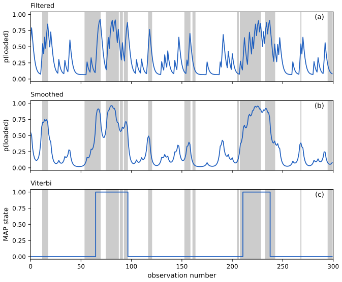
fig_9_3. Reproduces Murphy (2023), Figure 9.3. Download: PDF · SVG9.2.3.3 Two-slice smoothed marginals
Result 9.3 (two-slice marginals) p. 406, (9.20)–(9.29), Figure 9.4
\[ \xi_{t,t+1}(i,j)=p(z_t=i,z_{t+1}=j\given y_{1:T})\propto\alpha_t(i)A_{ij}\lambda_{t+1}(j)\beta_{t+1}(j) \tag{9.27} \], and \(\sum_j\xi_{t,t+1}(i,j)=\gamma_t(i)\), \(\sum_i\xi_{t,t+1}(i,j)=\gamma_{t+1}(j)\).
Proof
\[ p(z_t,z_{t+1}\given y_{1:T})\propto p(y_{t+1:T}\given z_t,z_{t+1},y_{1:t})\,p(z_t,z_{t+1}\given y_{1:t}) \]. Given \(z_{t+1}\) the future \(y_{t+1:T}\) does not depend on \(z_t\) or \(y_{1:t}\), so the first factor is \[ p(y_{t+1:T}\given z_{t+1})=\lambda_{t+1}(z_{t+1})\beta_{t+1}(z_{t+1}) \] (using \(y_{t+2:T}\perp y_{t+1}\given z_{t+1}\), (9.24)–(9.26)). The second factor is \[ p(z_t\given y_{1:t})p(z_{t+1}\given z_t)=\alpha_t(z_t)A_{z_tz_{t+1}} \]. Summing over either index recovers \(\gamma\) because both sides are normalised joint distributions of \((z_t,z_{t+1})\). The code confirms the identities and also that rows and columns sum to \(\gamma_t\) and \(\gamma_{t+1}\).
The matrix form (9.28) \[ \boldsymbol\xi_{t,t+1}\propto\mathbf{A}\odot(\boldsymbol\alpha_t(\boldsymbol\lambda_{t+1}\odot\boldsymbol\beta_{t+1})^\T) \] is the product of the four messages of Figure 9.4: the filtered belief, the transition, the local evidence and the backwards message. The two-slice marginals are the sufficient statistics for EM in an HMM (Baum–Welch, Algorithm 13.1 of the companion course).
9.2.3.4 Numerically stable implementation
p. 407 See Filling the gap 9.1.
9.2.4 Forwards filtering backwards smoothing
Result 9.4 (smoothing without \(\beta\)) pp. 407–408, (9.32)–(9.37)
If \(\alpha_{t+1|t}(j)>0\) for all \(j\), then with \(\gamma_T=\alpha_T\), \[ \xi_{t,t+1}(i,j)=\alpha_t(i)A_{ij}\frac{\gamma_{t+1}(j)}{\alpha_{t+1|t}(j)},\qquad \gamma_t(i)=\sum_j\xi_{t,t+1}(i,j). \tag{9.35, 9.37} \]
Proof
The key is \(p(z_t\given z_{t+1},y_{1:T})=p(z_t\given z_{t+1},y_{1:t})\): given \(z_{t+1}\), the future observations \(y_{t+1:T}\) carry no further information about \(z_t\). Then \[ p(z_t=i\given z_{t+1}=j,y_{1:t})=\frac{p(z_{t+1}=j\given z_t=i)p(z_t=i\given y_{1:t})}{p(z_{t+1}=j\given y_{1:t})}=\frac{A_{ij}\alpha_t(i)}{\alpha_{t+1|t}(j)}. \] Multiplying by \(\gamma_{t+1}(j)=p(z_{t+1}=j\given y_{1:T})\) gives \(\xi_{t,t+1}(i,j)\) (9.33)–(9.35), and marginalising \(j\) gives (9.37).
Comparison with (9.27): both are proportional in \(j\) to the same thing, because \[ \gamma_{t+1}(j)/\alpha_{t+1|t}(j)\propto\lambda_{t+1}(j)\beta_{t+1}(j) \] up to a factor not depending on \(j\) (indeed \(\gamma_{t+1}=\alpha_{t+1}\beta_{t+1}/c\) and \(\alpha_{t+1}=\lambda_{t+1}\alpha_{t+1|t}/Z_{t+1}\)). The code verifies numerically that FFBS and forwards-backwards agree to \(10^{-15}\). The division by \(\alpha_{t+1|t}\) is why FFBS is the method for continuous states (Kalman smoother, Chapter 8), where \(\beta\) is not a normalisable density.
9.2.5 Time and space complexity
pp. 408–409, (9.38), Figure 9.5 Each step multiplies a \(K\times K\) matrix by a vector, so time is \(O(K^2T)\) and space \(O(KT)\) (the filtered vectors are kept for the backwards pass). Three ways to do better are quoted:
- Sparse transitions. A left-to-right transition matrix has \(O(K)\) non-zeros, so \(O(KT)\) time.
- Convolution structure. If \(A_{ij}\propto\rho(z_j-z_i)\) on a grid, the predict step (9.5) is a convolution and the FFT gives \(O(TK\log K)\).
- Parallel prefix scan and checkpointing (memory \(O(K\log T)\) for time \(O(K^2T\log T)\), by storing \(\alpha,\beta\) at \(O(\log T)\) checkpoints and recomputing).
Filling the gap 9.2: the FFT form of the predict step and the scan form of the filter pp. 408–409
The book states the FFT trick without proof. If the states are arranged on a ring of \(K\) points and \(A_{ij}=\rho((j-i)\bmod K)\), then \(\alpha_{t|t-1}(j)=\sum_i\alpha_{t-1}(i)\rho((j-i)\bmod K)\) is the circular convolution of \(\alpha_{t-1}\) and \(\rho\). By the convolution theorem its discrete Fourier transform is the product of the transforms, \(\widehat{\alpha_{t|t-1}}=\hat\alpha_{t-1}\hat\rho\), and the FFT computes forward and inverse transforms in \(O(K\log K)\); \(\hat\rho\) is computed once. For a non-circular \(\rho\) on a line, pad the vectors with \(K\) zeros. The code checks equality with the matrix product for a \(64\)-state circulant (difference \(10^{-17}\)); the backwards pass is the same with the transposed kernel \(\rho(-u)\).
For the scan: the unnormalised filter is \(\alpha'_t=D_t\mathbf{A}^\T\alpha'_{t-1}\) with the diagonal \(D_t=\mathrm{diag}(\lambda_t)\), so \(\alpha'_T=(\prod_{t}M_t)\alpha'_0\) with \(M_t=D_t\mathbf{A}^\T\). Matrix multiplication is associative, so the \(T\) factors can be multiplied in a balanced tree (a parallel prefix scan) in \(O(\log T)\) parallel steps, at the price of \(K\times K\) matrix-matrix products (\(O(K^3)\) each) in place of matrix-vector products.
9.2.6 The Viterbi algorithm
pp. 409–411, (9.39)–(9.46), Figure 9.6 The MAP sequence \(z^*_{1:T}=\mathrm{arg\,max}\,p(z_{1:T}\given y_{1:T})\) maximises \[ \log\pi(z_1)+\log\lambda_1(z_1)+\sum_{t\ge2}[\log A(z_{t-1},z_t)+\log\lambda_t(z_t)] \]: a longest path through the trellis.
Result 9.5 (the Viterbi recursion) pp. 409–410, (9.42)–(9.45)
Let \(\delta_t(j)=\max_{z_{1:t-1}}p(z_{1:t-1},z_t=j,y_{1:t})\). Then \(\delta_1(j)=\pi_j\lambda_1(j)\), \(\delta_t(j)=\lambda_t(j)\max_i\delta_{t-1}(i)A_{ij}\) (9.43), and the ancestor \(a_t(j)=\mathrm{arg\,max}_i\delta_{t-1}(i)A_{ij}\) gives the MAP path by tracing back from \(z^*_T=\mathrm{arg\,max}_i\delta_T(i)\), \(z^*_t=a_{t+1}(z^*_{t+1})\).
Proof
\[ p(z_{1:t-1},z_t=j,y_{1:t})=\lambda_t(j)A_{z_{t-1}j}\,p(z_{1:t-1},y_{1:t-1}) \], and maximising first over \(z_{1:t-2}\) for a fixed \(z_{t-1}=i\) gives \(\delta_{t-1}(i)\) because the factor \(\lambda_t(j)A_{ij}\) does not involve \(z_{1:t-2}\) (maxima commute and non-negative factors can be moved out of a maximum). Then maximising over \(i\) gives (9.43). The maximum of the joint over all paths is \(\max_i\delta_T(i)\), attained at \(z^*_T\), and a path attaining it must pass through the maximiser \(a_T(z^*_T)\) at time \(T-1\) and so on (the traceback). In the log domain products become sums, \(\delta'_t=-\log\delta_t\), (9.44), which avoids underflow.
9.2.6.3 Example
pp. 410–411, (9.46)–(9.47), Figure 9.6 The 3-state left-to-right HMM has \[ A=\begin{pmatrix}0.3&0.7&0\\0&0.9&0.1\\0&0&0.4\end{pmatrix} \], start in \(S_1\), and emission probabilities of the codebook symbols C1..C7 as in the book's table. For the data \(C1,C3,C4,C6\): \[ \delta_1(1)=0.5,\ \ \delta_2(1)=0.5\cdot0.3\cdot0.3=0.045,\ \ \delta_2(2)=0.5\cdot0.7\cdot0.2=0.07,\] \[\delta_3(2)=\max(0.045\cdot0.7,\,0.07\cdot0.9)\cdot0.7=0.0441,\ \ \delta_3(3)=0.07\cdot0.1\cdot0.1=0.0007,\ \ \delta_4(3)=\max(0.0441\cdot0.1,\,0.0007\cdot0.4)\cdot0.5=0.002205, \] and the traceback gives the path \(S_1,S_2,S_2,S_3\), as in the book (the book's figure prints 0.0022 for the last value; the exact number is \(0.002205\)).
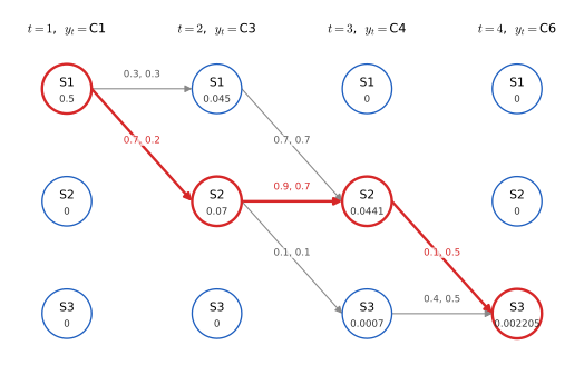
fig_9_6. Reproduces Murphy (2023), Figure 9.6(b). Download: PDF · SVG9.2.6.2 Backwards pass: MAP against the per-time maximiser
p. 410 The book says that with a unique MAP the traceback gives the same answer as \(\hat z_t=\mathrm{arg\,max}_j\gamma_t(j)\). That cannot be right as stated, and it is contradicted by Figure 9.3 itself, where the two methods make 60 and 49 errors; see the errata and Result 9.9 for the correct statement (the per-time maximiser of the max-marginals, not of the posterior marginals, equals the MAP).
9.2.6.4–9.2.6.5 Complexity and N-best lists
pp. 411–412 The cost is \(O(K^2T)\) time and \(O(KT)\) space (or \(O(TK)\) time for kernels \(\rho(z_j-z_i)\) by the generalised distance transform). Returning the top \(N\) paths (N-best list) costs a factor of about \(N\), but the paths are typically near-duplicates, which is the reason the book prefers posterior samples (next section).
9.2.7 Forwards filtering backwards sampling
Result 9.6 (exact joint samples) p. 412, (9.48)–(9.49)
Draw \(z_T\sim\alpha_T\), then for \(t=T-1,\dots,1\) draw \(z_t\) from \[ p(z_t=i\given z_{t+1},y_{1:T})\propto\alpha_t(i)A_{i,z_{t+1}} \]. The result is an exact sample from \(p(z_{1:T}\given y_{1:T})\), in \(O(TK)\) time after the filtering pass.
Proof
The chain rule from the right gives \[ p(z_{1:T}\given y_{1:T})=p(z_T\given y_{1:T})\prod_{t=T-1}^1p(z_t\given z_{t+1:T},y_{1:T}) \] (9.48). By the Markov property and the argument of Result 9.4, \[ p(z_t\given z_{t+1:T},y_{1:T})=p(z_t\given z_{t+1},y_{1:t})\propto\alpha_t(z_t)A_{z_t,z_{t+1}} \]. Sampling a sequence of variables from their successive conditionals is exact sampling from the joint. The code draws 40,000 paths for a 6-step HMM and compares with the exact posterior probability of each of the 64 paths: the largest deviation is 0.003, the size of Monte Carlo error.
9.3 Belief propagation on trees
p. 412 Forwards-backwards is message passing on a chain; here it is generalised to trees. The companion course proves sum-product on trees and factor graphs with Bishop's notation (Algorithm 8.4, Result 8.20, and max-sum with back-tracking, Result 8.22); the new points here are the pairwise-potential form, the division form of the downward message, and the relations between MAP, max-marginals and posterior marginals.
9.3.1 Directed vs undirected trees
pp. 412–413, (9.50)–(9.57), Figure 9.7 A pairwise model is \[ p^*(z)\propto\prod_{s\in V}\psi_s(z_s)\prod_{(s,t)\in E}\psi_{st}(z_s,z_t) \tag{9.50} \], with \(\psi_s(z_s)=\psi_s(z_s\given y_s)\) carrying the evidence.
Result 9.7 (a tree is directed or undirected, with node and edge marginals as potentials) pp. 413, (9.51)–(9.57)
If \(p^*\) is a distribution whose graph is a tree, then for any choice of root and orientation \[ p^*(z)=\prod_{s\in V}p^*(z_s)\prod_{(s,t)\in E}\frac{p^*(z_s,z_t)}{p^*(z_s)p^*(z_t)}=p^*(z_{r})\prod_{s\ne r}p^*(z_s\given z_{\mathrm{pa}(s)}). \tag{9.53, 9.56} \] Hence the undirected tree and every rooted directed version define the same family.
Proof
Induction on the number of nodes. For one node both sides are \(p^*(z_r)\). Let \(\ell\ne r\) be a leaf with neighbour \(m\) (the parent). The graph without \(\ell\) is a tree, and the Markov property of the tree gives \(z_\ell\perp z_{V\setminus\{\ell,m\}}\given z_m\), so \[ p^*(z)=p^*(z_{V\setminus\ell})\,p^*(z_\ell\given z_m)=p^*(z_{V\setminus\ell})\,\dfrac{p^*(z_\ell,z_m)}{p^*(z_m)} \]. By the induction hypothesis \(p^*(z_{V\setminus\ell})\) has the product form on the smaller tree. The new factor \[ p^*(z_\ell)\cdot\dfrac{p^*(z_\ell,z_m)}{p^*(z_\ell)p^*(z_m)} \] times the old product, with the extra \(p^*(z_m)\) cancelled, is exactly the product form for the bigger tree: each node has its marginal once and each edge its ratio once. The directed form follows by multiplying and dividing: \[ p^*(z_s)\cdot\dfrac{p^*(z_s,z_t)}{p^*(z_s)p^*(z_t)}=p^*(z_s\given z_t) \] re-orients any edge, which is the cancellation (9.54)–(9.57) written out for Figure 9.7. The code checks this identity for a random 4-node tree with different state-space sizes (difference \(10^{-17}\)).
9.3.2 Sum-product algorithm
pp. 414–415, (9.58)–(9.62), Figures 9.8–9.9 Root the tree at an arbitrary node. Let \(m_{s\to t}(z_t)\) summarise the evidence in the subtree on the \(s\) side of the edge. Collect (leaves to root, post-order): \[ \mathrm{bel}_s(z_s)\propto\psi_s(z_s)\prod_{t\in\mathrm{ch}_s}m_{t\to s}(z_s),\qquad m_{s\to t}(z_t)=\sum_{z_s}\psi_{st}(z_s,z_t)\,\mathrm{bel}_s(z_s)\ \ (t=\mathrm{pa}(s)). \tag{9.58, 9.59} \] Distribute (root to leaves, pre-order), where \(s\) is the parent of \(t\): \[ m_{s\to t}(z_t)=\sum_{z_s}\psi_s(z_s)\psi_{st}(z_s,z_t)\prod_{u\in\mathrm{nbr}_s\setminus t}m_{u\to s}(z_s)\tag{9.60}, \] where, for a non-root \(s\), the product includes the message \(m_{\mathrm{pa}(s)\to s}\) that \(s\) has just received from its parent (as printed, (9.60) lists only the other children, which is correct for the root; see the errata), and equivalently by dividing out the message that \(t\) sent up, \[ m_{s\to t}(z_t)=\sum_{z_s}\psi_{st}(z_s,z_t)\,\mathrm{bel}_s(z_s)/m_{t\to s}(z_s) \tag{9.61} \], followed by \(\mathrm{bel}_t\leftarrow\mathrm{bel}_t\cdot m_{s\to t}\) (9.62).
Algorithm (Figure 9.8): belief propagation on a pairwise rooted tree p. 414
- Collect to the root. For each node \(s\) in post-order: \[ \mathrm{bel}_s\propto\psi_s\prod_{t\in\mathrm{ch}_s}m_{t\to s} \]; \(t=\mathrm{pa}(s)\); \[ m_{s\to t}(z_t)=\sum_{z_s}\psi_{st}(z_s,z_t)\mathrm{bel}_s(z_s) \].
- Distribute from the root. For each node \(t\) in pre-order: \(s=\mathrm{pa}(t)\); \[ m_{s\to t}(z_t)=\sum_{z_s}\psi_{st}(z_s,z_t)\,\mathrm{bel}_s(z_s)/m_{t\to s}(z_s) \]; \[ \mathrm{bel}_t(z_t)\propto\mathrm{bel}_t(z_t)\,m_{s\to t}(z_t) \].
Result 9.8 (sum-product is exact on a tree; meaning of the messages; the division form) pp. 414–415, (9.58)–(9.62)
After the collect pass, \(\mathrm{bel}_s(z_s)\) is the sum, over all variables of the subtree \(\mathcal T_s\) below \(s\), of the product of all node and edge potentials of that subtree (with \(z_s\) fixed); \(m_{s\to t}(z_t)\) is the same with the edge potential \(\psi_{st}\) added and \(z_s\) summed out. After the distribute pass, \(\mathrm{bel}_t(z_t)\propto p^*(z_t)\), the exact marginal of the whole model, for every node \(t\). The division in (9.61) is legitimate whenever \(m_{t\to s}>0\) and gives the same message as the product over all neighbours of \(s\) other than \(t\).
Proof
Collect. Induction from the leaves. A leaf \(s\) has \(\mathrm{bel}_s=\psi_s\), the unnormalised \(p(z_s,y_s)\). Suppose each child \(t\) of \(s\) satisfies \[ m_{t\to s}(z_s)=\sum_{z_{\mathcal T_t}}\psi_{ts}\prod_{\text{nodes in }\mathcal T_t}\psi\prod_{\text{edges in }\mathcal T_t}\psi \] (the sum of the product of all potentials in the subtree and the edge to \(s\), over all variables of the subtree). The subtrees of different children share no variables, so the sum of the product over the union factorises into the product of the children's sums, and \(\mathrm{bel}_s\) in (9.58) equals the sum over all variables in \(\mathcal T_s\) other than \(z_s\) of the product of the potentials there. Then (9.59) adds the edge potential to the parent and sums out \(z_s\), which is the same statement for \(s\).
Distribute. Claim: when the parent \(s\) holds \(\mathrm{bel}_s\propto p^*(z_s)\), the message \(m_{s\to t}\) of (9.60) is proportional to the sum over all variables outside \(\mathcal T_t\) of the product of potentials outside \(\mathcal T_t\) and the edge potential, i.e. the evidence outside the subtree of \(t\); then \(\mathrm{bel}_t\) times it equals the sum over everything else of all potentials, \(\propto p^*(z_t)\). The tree structure makes the "outside" of \(\mathcal T_t\) a union of independent pieces (the siblings' subtrees and the parent's own outside), whose sums multiply to the product in (9.60), which uses the other children's messages and the message that came down to \(s\) (included in \(\mathrm{bel}_s\)). For (9.61): \[ \mathrm{bel}_s=\psi_s\prod_{u\in\mathrm{ch}_s}m_{u\to s}\cdot m_{\text{down}\to s} \], so dividing by \(m_{t\to s}\) removes exactly the factor of the child \(t\) from the product (division is legal when it is non-zero). The division has the interpretation given in the book: \(\mathrm{bel}_s\) is the new posterior of \(s\), \(m_{t\to s}\) is the old belief that \(t\)'s own subtree held, and their ratio is the new evidence that \(t\) has not seen.
The code implements both forms and compares with brute-force marginals of a random 7-node tree with 2–3 states per node, from three different roots (agreement \(10^{-16}\)).
BP for polytrees (supplement 9.1.1)
Supp. pp. 99–102, (S9.1)–(S9.24), Figure S9.1 A polytree is a directed graph whose undirected skeleton is a tree: nodes may have several parents. For a node \(X\) with parents \(U_i\) and children \(Y_j\), split the evidence into \(e^+_X\) (above \(X\)) and \(e^-_X\) (below and at \(X\)), and write \(\lambda_X(x)=p(e^-_X\given X=x)\), \(\pi_X(x)=p(X=x\given e^+_X)\), so that \(\mathrm{bel}_X(x)=p(x\given e)\propto\lambda_X(x)\pi_X(x)\) (S9.1).
Result 9.11 (Pearl's \(\lambda\)-\(\pi\) messages on a polytree) Supp. pp. 99–101, (S9.4)–(S9.24)
With the local evidence \(\lambda_{X\to X}(x)=p(e_X\given x)\), \begin{align} \lambda_X(x)&=\lambda_{X\to X}(x)\prod_j\lambda_{Y_j\to X}(x), & \pi_X(x)&=\sum_{\mathbf u}p(x\given\mathbf u)\prod_i\Pi_{U_i\to X}(u_i),\\ \lambda_{X\to U_i}(u_i)&\propto\sum_x\lambda_X(x)\sum_{u_k:k\ne i}p(x\given\mathbf u)\prod_{k\ne i}\Pi_{U_k\to X}(u_k), & \Pi_{X\to Y_j}(x)&\propto\pi_X(x)\lambda_{X\to X}(x)\prod_{k\ne j}\lambda_{Y_k\to X}(x), \end{align} (S9.6, S9.11, S9.22, S9.24). If the graph is a rooted tree (one parent), \(\lambda_{X\to U}(u)\propto\sum_x\lambda_X(x)p(x\given u)\) (S9.23). Sending messages along every edge in both directions gives the exact posterior of every node.
Proof
(i) \(\lambda_X\). Given \(X\), the evidence in the subtrees under the different children and the local evidence are conditionally independent (the polytree has no loops, so these pieces are separated by \(X\)), giving (S9.6). (ii) \(\pi_X\). Introduce the parents and use that, given \(U_1,U_2\), \(X\) is independent of everything above; the parents' upstream evidence pieces \(e^+_{U_i\to X}\) lie in disjoint subtrees and the parents are marginally independent (no common ancestor in a polytree), so \[ p(u_1,u_2\given e^+_{U_1\to X},e^+_{U_2\to X})=p(u_1\given e^+_{U_1\to X})p(u_2\given e^+_{U_2\to X}) \], which is (S9.7)–(S9.11). (iii) \(\lambda_{X\to U_1}\). The evidence not in the triangle above \(U_1\) is \((e^-_X,e^+_{U_2\to X})\). Sum over \(x,u_2\): \[ \lambda_{X\to U_1}(u_1)=\sum_x\sum_{u_2}p(e^-_X\given x)\,p(e^+_{U_2\to X}\given u_2)\,p(x,u_2\given u_1), \] using that \(X\) separates \(e^-_X\) from the rest and \(U_2\) separates its triangle. Since \(U_1\) and \(U_2\) are independent, \(p(x,u_2\given u_1)=p(x\given u_1,u_2)p(u_2)\), and Bayes' rule \[ p(e^+_{U_2\to X}\given u_2)p(u_2)=p(u_2\given e^+_{U_2\to X})\,p(e^+_{U_2\to X}) \] turns the right side into \[ c\sum_x\sum_{u_2}\lambda_X(x)\Pi_{U_2\to X}(u_2)p(x\given u_1,u_2) \] with the constant \(c=p(e^+_{U_2\to X})\), which is (S9.21); the general form is the same with all other parents. (iv) \(\Pi_{X\to Y_j}\). The evidence above the edge \(X\to Y_j\) is all evidence except the triangle below \(Y_j\), so \(\Pi_{X\to Y_j}(x)=p(x\given e\setminus e^-_{X\to Y_j})\), which is \(\mathrm{bel}_X\) with \(Y_j\)'s message left out: (S9.24). A two-pass protocol (to a root, then back) sends a message on each edge in each direction exactly once; against an arrow the message is a \(\lambda\), along it a \(\Pi\). For a rooted tree the first pass has only \(\lambda\) messages and the second only \(\Pi\) messages, as in the reversed forwards-backwards. The code implements these recursions and compares the posterior of every node of a random 7-node polytree (nodes with two parents, three local evidence vectors) with the enumeration of the joint: error \(10^{-16}\).
9.3.3 Max-product algorithm
pp. 415–417, (9.63)–(9.65) Replacing the sum by a maximum in the algorithm of Figure 9.8 gives the max-marginals \(\zeta_i(k)=\max_{z_{-i}}p(z_i=k,z_{-i}\given y)\) (9.64). The proof of Result 9.8 goes through unchanged, because it only uses that sums distribute over products; the same holds for max over non-negative numbers (see the semiring discussion in the generalised distributive law). Two estimates are made from the local quantities: the MPM (maximiser of the posterior marginal) \(\hat z_i=\mathrm{arg\,max}_k\gamma_i(k)\) and the MMM (maximiser of the max-marginal) \(\tilde z_i=\mathrm{arg\,max}_k\zeta_i(k)\).
9.3.3.1 Connection between MMM and MAP
Result 9.9 (MMM equals MAP when the maximiser is unique; ties and traceback) p. 416
If \(z^*=\mathrm{arg\,max}_zp(z\given y)\) is unique, then for every \(i\), \(\mathrm{arg\,max}_k\zeta_i(k)=z^*_i\) (Yanover and Weiss, 2004), so \(\tilde z=z^*\). If there are several maximisers, the MMM can combine pieces of different ones and fail to be a maximiser; a traceback (as in Viterbi) or clamping repairs this. In particular the per-time maximiser of the posterior marginals is not the MAP.
Proof
Fix \(i\). \[ \zeta_i(z^*_i)=\max_{z_{-i}}p(z^*_i,z_{-i}\given y)\ge p(z^*\given y) \], and \(p(z^*\given y)=\max_zp(z\given y)\ge\zeta_i(k)\) for every \(k\) (each \(\zeta_i(k)\) is the maximum of \(p\) over a subset of configurations). So \(\zeta_i(z^*_i)=p(z^*\given y)\) is the global maximum. For \(k\ne z^*_i\) the maximum \(\zeta_i(k)\) is attained by some configuration with \(z_i=k\), which is not \(z^*\); uniqueness makes that value strictly smaller than \(p(z^*\given y)\). Hence \(z^*_i\) is the unique maximiser of \(\zeta_i\). With ties the statement fails: in the error-correcting example below all max-marginals are equal (0.3265) so the MMM is undefined, and with a second MAP \(z'\) different from \(z^*\) one may pick \(z^*_1\) and \(z'_2\) from the two and obtain a non-maximiser. A traceback starts at the root with a maximiser and, going away from the root, picks the child values consistent with the one chosen (Viterbi's ancestor pointers), so every node breaks ties compatibly. On general graphs traceback is not available; Yanover and Weiss's iterative fix clamps the nodes with unique max-marginals and re-runs.
The statement about posterior marginals: the per-time maximiser of \(\gamma\) is the MPM, not the MMM. For the casino sample of Figure 9.3 the MPM path and the Viterbi path differ at several positions, and for 35 of 40 further random sequences of length 60 they differ somewhere (checked in the code).
9.3.3.2 Connection between MPM and MAP
pp. 416–417, Section 5.5 example The error-correcting example: \[ p(z_1,z_2,z_3,y)=p(z_1)p(z_2)p(z_3\given z_1,z_2)\prod_{i=1}^3p(y_i\given z_i) \] with uniform priors on \(z_1,z_2\), \(z_3=z_1\oplus z_2\) deterministic (the parity of \((z_1,z_2)\)), and a bit-flip channel with flip probability \(\alpha=0.2\). Only the four codewords \(000,011,101,110\) have positive probability (prior \(1/4\) each). For \(y=(1,0,0)\): \[ \begin{array}{c|ccc} \text{codeword}&000&011&101&110\\\hline \text{likelihood}&0.2\cdot0.8\cdot0.8=0.128&0.2^3=0.008&0.8\cdot0.8\cdot0.2=0.128&0.8\cdot0.2\cdot0.8=0.128 \end{array} \] The normaliser is \(0.392\). Then \[ p(z_1=1\given y)=(0.128+0.128)/0.392=0.6531 \], \[ p(z_2=1\given y)=(0.008+0.128)/0.392=0.3469 \] and \(p(z_3=1\given y)=0.3469\), the marginals \(\gamma_1=[0.3469,0.6531]\), \(\gamma_2=[0.6531,0.3469]\), \(\gamma_3=[0.6531,0.3469]\) of the book. Every max-marginal is \(0.128/0.392=0.3265\) for both values of every bit, so the MMM is undefined; the three MAP words are \(000,101,110\) (one flip away from \(y\)). The MPM estimate is \(\hat z=(1,0,0)\) (take the larger marginal in each position), which is not a codeword (odd weight).
Result 9.10 (MPM minimises the expected number of bit errors, MAP the probability of a wrong word) p. 417; Section 34.1
For the loss \(\sum_i\mathbb 1[\hat z_i\ne z_i]\) (bit error) the Bayes decision is \(\hat z_i=\mathrm{arg\,max}_k\gamma_i(k)\); for the loss \(\mathbb 1[\hat z\ne z]\) (word error) it is \(z^*=\mathrm{arg\,max}_z p(z\given y)\).
Proof
Expected bit error of \(\hat z\) is \(\sum_i(1-\gamma_i(\hat z_i))\), minimised coordinate-wise by the largest \(\gamma_i(\hat z_i)\). Expected word error is \(1-p(\hat z\given y)\), minimised by the mode. The code checks both statements on 600 random casino sequences of length 20: the mean number of bit errors is lower for MPM (4.06) than for Viterbi (4.52), and the posterior probability of the Viterbi path is at least that of the MPM path every time. In the casino problem the MPM wins on the bit-error measure (51 against 57 errors in our sample, 49 against 60 in the book's), while in the code example the MPM is not even a legal word.
9.3.3.3 Connection between MPE and MAP
p. 417, (9.65) In the graphical-models literature the jointly most probable setting \(z^*\) is called the most probable explanation (MPE) and "MAP" means: maximise a subset \(Q\) of the variables and sum out the rest \(R\): \[ z^*_Q=\mathrm{arg\,max}_{z_Q}\sum_{z_R}p(z_Q,z_R\given z_V) \] (9.65). The book calls this an MPM estimate to avoid the clash with the machine-learning meaning of MAP. For \(Q=\{i\}\) it is the single-node MPM; for \(Q=\) all hidden nodes it is the MPE. Note that this mixed problem (max over some, sum over the rest) is harder than either pure problem and is not solved by one pass of message passing.
9.4 Loopy belief propagation
pp. 417–418 Pearl introduced belief propagation for trees and warned that on graphs with loops the messages may circulate and not settle, and that if they do the result need not be the posterior. Empirically (Murphy, Weiss and Jordan, 1999) it nevertheless often works, and it is the algorithm behind turbo and LDPC decoding. There is also theory: Result 9.12 (computation trees), Result 9.13 (convergence for weak couplings) and Result 9.14 (Gaussian means).
9.4.1 Loopy BP for pairwise undirected graphs
p. 418, (9.66)–(9.67) Initialise all messages to the all-ones vector. In parallel every node absorbs and sends: \[ \mathrm{bel}_s(z_s)\propto\psi_s(z_s)\prod_{t\in\mathrm{nbr}_s}m_{t\to s}(z_s),\qquad m_{s\to t}(z_t)=\sum_{z_s}\psi_s(z_s)\psi_{st}(z_s,z_t)\prod_{u\in\mathrm{nbr}_s\setminus t}m_{u\to s}(z_s). \tag{9.66, 9.67} \] Repeat until no message changes. On a tree the method converges after \(D(G)\) iterations, the diameter.
Result 9.12 (the computation tree; exactness on trees after \(D\) sweeps) pp. 418, 421, Figure 9.12
Start synchronous BP from uniform messages. After \(T\) sweeps the belief at node \(r\) equals the exact marginal of \(r\) in the computation tree of depth \(T\): the root \(r\), its children the neighbours of \(r\), and recursively each node's children are its neighbours except its parent, down to depth \(T\); every copy of a node carries the potential \(\psi_s\) and every edge the potential \(\psi_{st}\). If the graph is a tree, the computation tree of depth \(D\) contains each original node exactly once on every path, so the beliefs are exact after \(D\) sweeps, and (generically) not before.
Proof
Induction on \(T\). For \(T=0\) the belief is \(\psi_r\), the marginal of a one-node tree. A message \(m^T_{s\to t}\) is computed from \(\psi_s\), \(\psi_{st}\) and the messages \(m^{T-1}_{u\to s}\), \(u\ne t\). By induction \(m^{T-1}_{u\to s}\) is the sum-product message that the root of the depth-\((T-1)\) computation subtree below the edge \(u\to s\) sends to its parent; those subtrees of different \(u\) are disjoint pieces of the depth-\(T\) tree. Assembling them under \(s\) shows that \(m^T_{s\to t}\) is the sum-product message in the computation tree (Result 9.8), and the belief is the product of the messages into the root, hence the root marginal of the computation tree. In a tree graph the computation tree of depth \(D\) is the original tree unrolled, in which each node appears once when the root is a leaf at the longest distance; nodes at distance less than \(D\) are reached by messages in fewer steps, and the farthest pair is exactly \(D\) apart, so the farthest evidence arrives at sweep \(D\) and not earlier. The code builds the computation trees for the 4-node graph of Figure 9.12 (edges 12, 13, 23, 24, 34) with random potentials and checks that the root belief of sweeps \(T=1,\dots,4\) equals the exact marginal of the corresponding tree (error \(10^{-16}\)); for a 9-node chain of diameter 8 with strong couplings the beliefs are exact to \(10^{-16}\) after 8 sweeps and still wrong by \(10^{-8}\) after 7.
In Figure 9.12's example the second iteration at node 1 receives one message from node 3 (via 2), one from 2 (via 3) and two from 4 (via 2 and via 3), because nodes 2 and 3 have degree 3.
9.4.2 Loopy BP for factor graphs
pp. 418–419, (9.68)–(9.70), Figure 9.10 For factors \(f\) of any arity, the bipartite factor graph has variable-to-factor and factor-to-variable messages \[ m_{x\to f}(x)=\prod_{h\in\mathrm{nbr}(x)\setminus f}m_{h\to x}(x),\quad m_{f\to x}(x)=\sum_{\mathbf x'}f(x,\mathbf x')\prod_{x'\in\mathrm{nbr}(f)\setminus x}m_{x'\to f}(x'),\quad \mathrm{bel}(x)\propto\prod_{f\in\mathrm{nbr}(x)}m_{f\to x}(x). \tag{9.68, 9.69, 9.70} \] The schedule can be a flood (all at once), a spanning-tree order or residual BP (Section 9.4.4.3). The proofs of exactness on trees are those of the companion course (Result 8.20); see also factor graphs in Chapter 4. The code runs the flooding schedule on a factor graph containing a three-variable factor and gets the exact marginals of a tree-shaped factor graph (the 3-bit code of Section 9.3.3.2 is a second example: error \(10^{-16}\)).
9.4.3 Gaussian belief propagation
pp. 419–421, (9.71)–(9.76), Figure 9.11 For a Gaussian MRF \(p(x)\propto\exp(-\tfrac12x^\T Jx+h^\T x)\) with precision \(J\) and shift \(h\), the mean \(\mu=J^{-1}h\) solves a linear system, so BP also solves linear equations.
Result 9.14 (Gaussian BP: messages, and exact means at a fixed point) p. 419, Section 9.4.5
Messages are Gaussian potentials \(\exp(-\tfrac12P_{i\to j}x_j^2+m_{i\to j}x_j)\) with \[ P_{i\to j}=-\frac{J_{ij}^2}{a_{i\setminus j}},\quad m_{i\to j}=-\frac{J_{ij}\,b_{i\setminus j}}{a_{i\setminus j}},\qquad a_{i\setminus j}=J_{ii}+\sum_{k\ne j}P_{k\to i},\ b_{i\setminus j}=h_i+\sum_{k\ne j}m_{k\to i}. \] The belief of node \(i\) has precision \(P_i=J_{ii}+\sum_kP_{k\to i}\) and mean \(\mu_i=(h_i+\sum_km_{k\to i})/P_i\). On a tree these are the exact marginals. On a graph with loops, if the messages converge to a fixed point with \(a_{i\setminus j}a_{j\setminus i}\ne J_{ij}^2\) for all edges, the means \(\mu_i\) are exact: \(J\mu=h\). The variances \(1/P_i\) are in general not exact.
Proof
Messages. Integrating \(x_i\) out of \(\exp(-\tfrac12ax_i^2+bx_i-J_{ij}x_ix_j)\) (the factor of node \(i\) with its other incoming messages, times the cross term of the exponent) completes the square: \[ \int\exp(-\tfrac12ax_i^2+(b-J_{ij}x_j)x_i)\,dx_i\propto\exp((b-J_{ij}x_j)^2/(2a)) \], whose \(x_j\)-dependent part is \(\exp(\tfrac12(J_{ij}^2/a)x_j^2-(J_{ij}b/a)x_j)\), i.e. \(P=-J_{ij}^2/a\) and \(m=-J_{ij}b/a\).
Exact means at a fixed point. Write \(a=a_{i\setminus j}\), \(a'=a_{j\setminus i}\), \(x=J_{ij}\), \(b=b_{i\setminus j}\), \(b'=b_{j\setminus i}\), and define the edge residual \(r_{ij}=a\mu_i+x\mu_j-b\). Since \(P_j=a'+P_{i\to j}\) and \(P_j\mu_j=b'+m_{i\to j}\) we get \[ a'\mu_j=b'+m_{i\to j}-P_{i\to j}\mu_j=b'-xb/a+(x^2/a)\mu_j \]. Hence \[ r_{ji}:=a'\mu_j+x\mu_i-b'=\frac{x}{a}\,(a\mu_i+x\mu_j-b)=\frac xa\,r_{ij}, \] and by symmetry \(r_{ij}=\dfrac{x}{a'}r_{ji}\). Therefore \(r_{ji}(1-x^2/(aa'))=0\) and \(r_{ji}=0\) when \(aa'\ne x^2\). Now \(J_{ii}\mu_i+\sum_jJ_{ij}\mu_j-h_i\), using \(h_i=P_i\mu_i-\sum_jm_{j\to i}\) and \(P_i=J_{ii}+\sum_jP_{j\to i}\), equals \(\sum_j[x_j\mu_j+m_{j\to i}-P_{j\to i}\mu_i]\), and with \(m_{j\to i}=-x_jb'_j/a'_j\), \(P_{j\to i}=-x_j^2/a'_j\) each bracket is \((x_j/a'_j)\,r_{ji}=0\). So \(J\mu=h\). (On a tree the fixed point is reached after \(D\) sweeps, Result 9.12, and the marginals are exact by Result 9.8.)
The code confirms the residual identity numerically: on a \(6\times6\) Gaussian grid (diagonal 4.5, neighbours \(-1\)) \(\|J\mu-h\|_\infty<10^{-10}\) at convergence.
Filling the gap 9.3: the interpolation model of Figure 9.11 pp. 420–421, (9.71)–(9.76)
The book writes the measurement and smoothness terms as squared errors "\(\psi_i=(\hat y_i-y_i)^2/\sigma^2\)", which are energies, not potentials. The potentials are \(\psi_i=\exp\{-(\hat y_i-y_i)^2/(2\sigma^2)\}\) and \(\varphi_i=\exp\{-(z_i-z_{i-1})^2/(2\tau^2)\}\), so the model is the Gaussian MRF with \[ J=\sum_i\mathbf v_i\mathbf v_i^\T/\sigma^2+\sum_i\mathbf d_i\mathbf d_i^\T/\tau^2 \] and \(h=\sum_iy_i\mathbf v_i/\sigma^2\), where \(\mathbf v_i\) has entries \(1-\gamma_i,\gamma_i\) at the two grid points around the \(i\)th measurement and \(\mathbf d_i=(\dots,-1,1,\dots)\). The interpolation weight (9.73) is printed as \(\gamma_i=(x_i-g_i)/(g_i-g_{i-1})\); for a measurement between \(g_{i-1}\) and \(g_i\) this lies in \([-1,0]\), and the prediction \((1-\gamma_i)z_{i-1}+\gamma_iz_i\) would then have weights outside \([0,1]\), so it must be \(\gamma_i=(x_i-g_{i-1})/(g_i-g_{i-1})\). Since \(J\) is tridiagonal (a chain) Gaussian BP is exact, a Kalman-smoother-like computation. The figure below uses 14 noisy readings (\(\sigma=0.12\)) of a sine wave, 40 grid intervals on \([0,10]\) and \(\tau=0.35\); BP converges in 30 sweeps to the direct solution \(J^{-1}h\) (difference \(10^{-13}\)), with a posterior standard deviation that grows away from the data and, with a random-walk smoothness prior, a mean that is flat beyond the last reading.
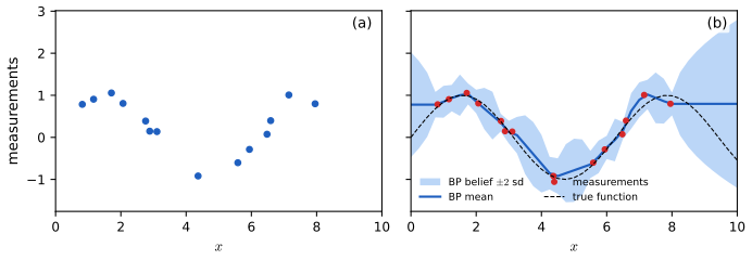
fig_9_11. Reproduces Murphy (2023), Figure 9.11. Download: PDF · SVGFor non-linear Gaussian factors the book points to extended Kalman and sigma-point versions on factor graphs (Chapter 8) and for non-Gaussian messages to particle BP (Chapter 13).
9.4.4 Convergence
9.4.4.1 When will LBP converge?
p. 421 By Result 9.12 \(T\) sweeps of BP are exact inference in the computation tree of depth \(T\). If the edge couplings are weak, the influence of the leaves on the root shrinks with depth, so the beliefs stop changing. A precise version for binary pairwise models:
Result 9.13 (BP is a contraction under weak coupling) p. 421; Mooij and Kappen (2007) for the proof technique
Take \(z_i\in\{-1,+1\}\), \(\psi_s(z_s)=e^{h_sz_s}\), \(\psi_{st}=e^{w_{st}z_sz_t}\), let \(d\) be the maximum degree and \(t^*=\max|\tanh w_{st}|\). In the cavity-field parametrisation \[ u_{s\to t}=\tfrac12\log\frac{m_{s\to t}(+1)}{m_{s\to t}(-1)} \] the synchronous update is \[ u_{s\to t}=\operatorname{atanh}(\tanh w_{st}\tanh(h_s+\sum_{k\ne t}u_{k\to s})) \]. If \(t^*(d-1)<1\), this map is a contraction in the sup norm with factor \(t^*(d-1)\): the BP fixed point is unique and synchronous BP converges to it from any initial messages, geometrically.
Proof
The message \(m_{s\to t}\) from (9.67) has log-ratio \[ \log\frac{\sum_{z_s}e^{z_s(\cdot)}e^{w z_s}}{\sum_{z_s}e^{z_s(\cdot)}e^{-wz_s}} \]; evaluating the sums gives \(2\operatorname{atanh}(\tanh w\tanh\phi)\) with \(\phi=h_s+\sum_{k\ne t}u_{k\to s}\) (the cavity field), i.e. the formula above after halving. Let \(g(\phi)=\operatorname{atanh}(\theta\tanh\phi)\) with \(\theta=\tanh w\). Then \[ g'(\phi)=\frac{\theta(1-\tanh^2\phi)}{1-\theta^2\tanh^2\phi}, \] and since \(1-\tanh^2\phi\le1-\theta^2\tanh^2\phi\) for \(|\theta|\le1\), \(|g'(\phi)|\le|\theta|\le t^*\). By the mean value theorem, for two message vectors \(u,\tilde u\), \[ |u_{s\to t}^{new}-\tilde u^{new}_{s\to t}|\le t^*\sum_{k\ne t}|u_{k\to s}-\tilde u_{k\to s}|\le t^*(d-1)\|u-\tilde u\|_\infty \]. A contraction of the complete metric space has a unique fixed point and the iterates converge geometrically (Banach). In the code the grid has \(d=4\), so the bound is \(|w|<\operatorname{atanh}(1/3)=0.3466\); with couplings uniform in \([-0.329,0.329]\) two very different starting messages (initial log-odds distance 3.7) are \(8\times10^{-7}\) apart after 10 sweeps, below the guaranteed \(0.95^{10}\times3.7=2.2\), and both end at the same fixed point (\(10^{-10}\)).
The condition is sufficient, not necessary: the grid of Figure 9.13 has couplings up to 1.7 and BP converges, with damping and the right schedule, nonetheless.
9.4.4.2 Making LBP converge
pp. 421–422, (9.77), Figure 9.13 Damping: \[ m^k_{t\to s}=\lambda\,m_{t\to s}+(1-\lambda)m^{k-1}_{t\to s} \], with \(m_{t\to s}\) the undamped message, \(\lambda=1\) the standard scheme and \(\lambda\approx0.5\) typical.
Filling the gap 9.4: damping keeps the fixed points p. 422, (9.77)
Write the undamped update as \(m\mapsto F(m)\). A damped step is \(m\mapsto(1-\lambda)m+\lambda F(m)\). For \(\lambda\in(0,1]\), \[ m=(1-\lambda)m+\lambda F(m)\iff\lambda m=\lambda F(m)\iff m=F(m) \], so the fixed points, and hence the beliefs BP converges to, are exactly those of the undamped iteration: damping only changes the dynamics, not the answer. Near a fixed point the iteration matrix changes from \(DF\) to \((1-\lambda)I+\lambda DF\), so an eigenvalue \(\mu\) of \(DF\) becomes \(1-\lambda+\lambda\mu\); an eigenvalue \(\mu\) with \(|\mu|>1\) can be moved inside the unit disk when \(\mu\) is real and negative (the typical oscillation) by taking \(\lambda<2/(1-\mu)\), but not when \(\mu>1\). This is why damping cures oscillations but not a fixed point that is unstable in the other direction. The code verifies numerically that damped, undamped, synchronous, asynchronous and residual schedules end at the same fixed point (difference \(10^{-9}\)) when the couplings are weak, and that the final messages satisfy (9.67) to \(10^{-13}\).
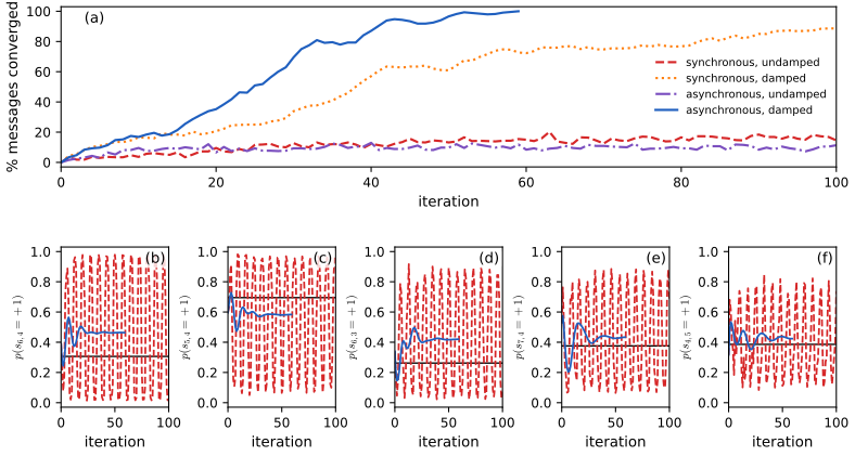
fig_9_13. Reproduces Murphy (2023), Figure 9.13. Download: PDF · SVGThe double-loop algorithms of Yuille (2002) and Welling and Teh (2001) are guaranteed to converge to a local minimum of the Bethe free energy but are slow; oscillation is sometimes a sign that the Bethe approximation itself is poor.
9.4.4.3 Increasing the convergence rate with adaptive scheduling
p. 423, (9.78)–(9.80) Synchronous updates \(m^{k+1}_{1:E}=(f_1(m^k),\dots,f_E(m^k))\) are the Jacobi method; asynchronous updates \(m^{k+1}_i=f_i(\{m^{k+1}_j\}_{j<i},\{m^k_j\}_{j>i})\) are Gauss–Seidel (9.79). Residual BP (Elidan, McGraw and Koller, 2006) sends next the message with the largest residual \(r(s,t,k)=\|\log m_{s\to t}-\log m^k_{s\to t}\|_\infty\) (9.80), kept in a priority queue; after a message \(s\to t\) is sent only the messages \(t\to u\), \(u\ne s\), need their residuals recomputed. All three schedules have the same fixed points as synchronous BP (they are different ways of looking for solutions of \(m=F(m)\)); the code implements the three and obtains the same beliefs on a weakly coupled grid.
9.4.5 Accuracy
pp. 423–424 For a graph with a single loop the max-product version finds the correct MAP if it converges (Weiss, 2000); the code tests this on 20 random 6-cycles with frustrated couplings and finds no counterexample (whenever max-product converged, its decoding was the MAP). For general graphs the errors of the beliefs can be bounded (Wainwright et al. 2003, Ihler et al. 2005). For Gaussians, Result 9.14 shows that the means are exact whenever BP converges; the variances are typically over-confident. Figure 9.S2 shows this on a \(6\times6\) Gaussian grid with diagonal 4.5 and neighbour entries \(-1\): the means converge geometrically to the exact ones (error \(10^{-12}\) after 64 sweeps), and the belief variances are between 0.934 and 0.989 times the exact variances.
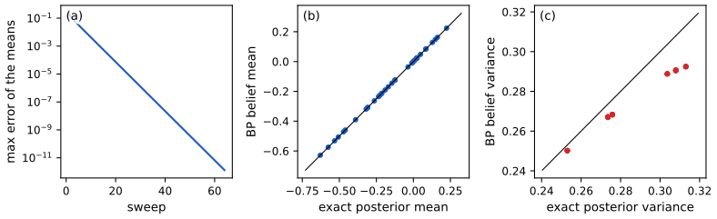
fig_9_S2. Download: PDF · SVG9.4.6 Generalized belief propagation
p. 424, Figure 9.14 Clustering nodes that form tight loops gives the cluster variational method of Yedidia, Freeman and Weiss (2000): messages between clusters of a hyper-graph (a poset of regions ordered by inclusion). If the largest region is as big as the treewidth the hyper-graph is a junction tree and the method is exact, so there is a continuum of approximations from loopy BP (regions of size 2) to the exact junction tree algorithm (Section 9.6). The variational derivation is in Chapter 10 (notes).
9.4.7 Convex BP
p. 424 The Bethe free energy that loopy BP minimises is non-convex; the tree-reweighted (convex) version always converges and is the LP-relaxation message-passing algorithm for MAP (supplement 9.3.3); see Chapter 10.
9.4.8 Application: error correcting codes
pp. 424–426, (9.81), Figure 9.15 A message \(x\in\{0,1\}^m\) is sent through a noisy channel and the receiver computes \(x^*=\mathrm{arg\,max}_xp(x\given y)\). The prior is the uniform distribution on the codewords, a factor graph with one parity factor per check, \(\psi(x_s,x_t,x_u)=\mathbb 1[x_s\oplus x_t\oplus x_u=0]\) (the book prints "\(=1\)", see the errata), plus one local evidence factor per bit. An \((n,k)\) code has every bit in \(n\) checks and every check on \(k\) bits; with bounded degrees as the block length grows it is a low-density parity check (LDPC) code. Random sparse factor graphs are locally tree-like (cycles of length about \(\log m\)), which is the heuristic reason loopy BP works well; McEliece, MacKay and Cheng (1998) showed that turbo decoding is an instance of loopy BP.
Filling the gap 9.5: the check-node message is the tanh rule pp. 424–426
For a binary variable write the message to a check as a log-likelihood ratio \(\ell=\log\frac{m(0)}{m(1)}\); then \(\tanh(\ell/2)=m(0)-m(1)\) for a normalised message. For a parity check on bits \(x_1,\dots,x_k\) with incoming normalised messages \(q_i\), the message to bit \(x_1\) is, by (9.69), proportional to \[ \sum_{x_2,\dots,x_k}\mathbb 1[x_2\oplus\dots\oplus x_k=x_1]\prod_{i\ge2}q_i(x_i)=\Pr[X_2\oplus\dots\oplus X_k=x_1] \] with independent \(X_i\sim q_i\). Let \(E=(-1)^{X_2\oplus\dots\oplus X_k}=\prod_{i\ge2}(-1)^{X_i}\). By independence \[ \mathbb E[E]=\prod_{i\ge2}\mathbb E[(-1)^{X_i}]=\prod_{i\ge2}(q_i(0)-q_i(1)) \], and \(\mathbb E[E]=\Pr[\text{even}]-\Pr[\text{odd}]\). Hence the message to \(x_1\) has \(m(0)-m(1)=\prod_{i\ge2}\tanh(\ell_i/2)\), that is \[ \ell_{c\to1}=2\operatorname{atanh}(\prod_{i\ge2}\tanh(\ell_i/2)). \] A variable-to-check message is the channel LLR plus the other checks' messages (a sum, from (9.68)). For a binary symmetric channel with flip probability \(p\) the channel LLR is \(\pm\log\frac{1-p}p\). The code implements this decoder with exclusive products by prefix and suffix products (no division), and checks that for a small code its hard decisions equal those of the generic factor-graph BP of (9.68)–(9.70) on the same parity factors.
As a demonstration, Figure 9.S1 decodes a random \((3,6)\) LDPC code (rate \(1/2\), block lengths 504 and 1008) over a binary symmetric channel, using the all-zero codeword (enough because the channel is symmetric and the decoder is symmetric). At flip probability \(p=0.05\) the uncoded bit error rate is 0.05, BP reduces it to \(10^{-4}\) (block length 504), and the frame error rate is 0.5%; at \(p=0.07\) the bit error rate is 1.3% for 504 bits and 0.7% for 1008 bits, and the capacity limit of rate \(1/2\), \(p=0.110\), is not reached by this short code. The decoder was never designed for loopy graphs, yet it works far beyond what the zero-loop analysis could justify.
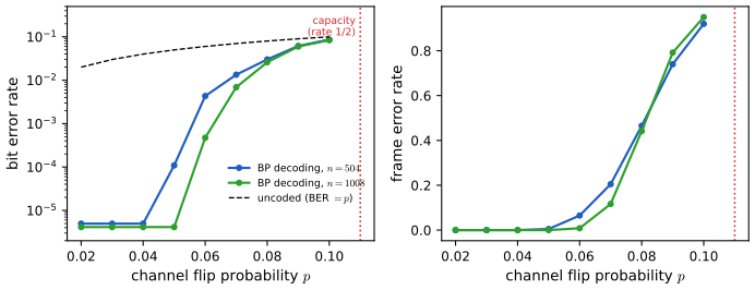
fig_9_S1. Download: PDF · SVG9.4.9 Application: affinity propagation
pp. 426–427, (9.82)–(9.83), Figures 9.16–9.17 Each data point \(i\) chooses an exemplar \(c_i\in\{1,\dots,N\}\); maximise \(J(c)=\sum_iS(i,c_i)+\sum_k\delta_k(c)\) (9.82), where \(S\) is a similarity and \(\delta_k(c)=-\infty\) if \(c_k\ne k\) but some \(c_i=k\), else 0 (9.83). The number of clusters is controlled by the diagonal \(S(k,k)\), the "preferences". The factor graph has variables \(c_i\) (each with \(N\) states) joined to local factors \(e^{S(i,\cdot)}\) and to the \(N\) constraint factors \(\delta_k\). The book says that the max-product messages "reduce to scalars"; this is the derivation.
Result 9.15 (affinity propagation is max-product BP) p. 426
Max-product BP on this factor graph is equivalent to the updates \[ r(i,k)\leftarrow S(i,k)-\max_{k'\ne k}[a(i,k')+S(i,k')],\qquad a(i,k)\leftarrow\min\{0,\ r(k,k)+\sum_{i'\notin\{i,k\}}\max\{0,r(i',k)\}\}\ (i\ne k), \] \[ a(k,k)\leftarrow\sum_{i'\ne k}\max\{0,r(i',k)\}, \] where \(r(i,k)\) (responsibility) is the log-message difference sent from \(c_i\) to \(\delta_k\) and \(a(i,k)\) (availability) the one sent from \(\delta_k\) to \(c_i\). The current choice is \(c_i=\mathrm{arg\,max}_k[a(i,k)+S(i,k)]\) and \(k\) is an exemplar when \(a(k,k)+r(k,k)>0\).
Proof
Work with log-messages (max-sum). Let \(\mu_{i\to k}(c)\) be the message from \(c_i\) to \(\delta_k\): \(\mu_{i\to k}(c)=S(i,c)+\sum_{k'\ne k}\nu_{k'\to i}(c)\), where \(\nu_{k'\to i}\) is the message from \(\delta_{k'}\) to \(c_i\). Take \(i\ne k\). The factor \(\delta_k\) only distinguishes whether \(c_i=k\) or not, so \(\nu_{k\to i}(c)\) takes one value \(\nu(k)\) when \(c=k\) and one value \(\nu(\ne k)\) otherwise. Maximise over the other variables \(c_j\), \(j\ne i\): \begin{align*} \nu(k)&=\mu_{k\to k}(k)+\sum_{j\ne i,k}\max_c\mu_{j\to k}(c)&&(c_i=k\Rightarrow c_k=k\text{ is required}),\\ \nu(\ne k)&=\max\{\mu_{k\to k}(k)+\sum_{j\ne i,k}\max_c\mu_{j\to k}(c),\ \max_{c\ne k}\mu_{k\to k}(c)+\sum_{j\ne i,k}\max_{c\ne k}\mu_{j\to k}(c)\}, \end{align*} the two branches being \(c_k=k\) (anyone may choose \(k\)) and \(c_k\ne k\) (then no \(c_j\) may equal \(k\)). Messages are only defined up to an additive constant, so keep the difference \(a(i,k)=\nu(k)-\nu(\ne k)=\min\{0,\Delta\}\) with \[ \Delta=[\mu_{k\to k}(k)-\max_{c\ne k}\mu_{k\to k}(c)]+\sum_{j\ne i,k}[\max_c\mu_{j\to k}(c)-\max_{c\ne k}\mu_{j\to k}(c)]. \] Define the responsibility \(r(j,k)=\mu_{j\to k}(k)-\max_{c\ne k}\mu_{j\to k}(c)\). Then \[ \max_c\mu_{j\to k}(c)-\max_{c\ne k}\mu_{j\to k}(c)=\max\{0,r(j,k)\} \], which gives the availability formula. For \(i=k\): \(\nu_{k\to k}(k)=\sum_{j\ne k}\max_c\mu_{j\to k}(c)\) and \[ \nu_{k\to k}(\ne k)=\sum_{j\ne k}\max_{c\ne k}\mu_{j\to k}(c) \], whose difference is \(\sum_{j\ne k}\max\{0,r(j,k)\}=a(k,k)\). For the responsibility, substitute: because each \(\nu_{k'\to i}(c)\) equals a constant plus \(a(i,k')\mathbb 1[c=k']\), we have \(\mu_{i\to k}(c)=S(i,c)+a(i,c)\) plus a constant for \(c\ne k\), (the term \(k'=c\) is present because \(c\ne k\)), hence \[ r(i,k)=\mu_{i\to k}(k)-\max_{c\ne k}\mu_{i\to k}(c)=S(i,k)-\max_{c\ne k}[S(i,c)+a(i,c)] \]. The final decision of \(c_i\) is the argmax of the belief \[ S(i,c)+\sum_{k'}\nu_{k'\to i}(c)=S(i,c)+a(i,c)+\mathrm{const} \], and \(c_k=k\) beats all alternatives iff \[ S(k,k)+a(k,k)>\max_{c\ne k}[S(k,c)+a(k,c)]\iff r(k,k)+a(k,k)>0 \].
Implementation check: the code runs these updates with damping 0.5 and, on 120 points drawn from three Gaussian blobs, with the median pairwise similarity as preference, finds 3 exemplars after 45 iterations; the partition equals the one a standard library implementation of the same algorithm produces. Each iteration costs \(O(N^2)\) (or \(O(E)\) with a sparse similarity matrix); the method may oscillate and damping makes it reliable.
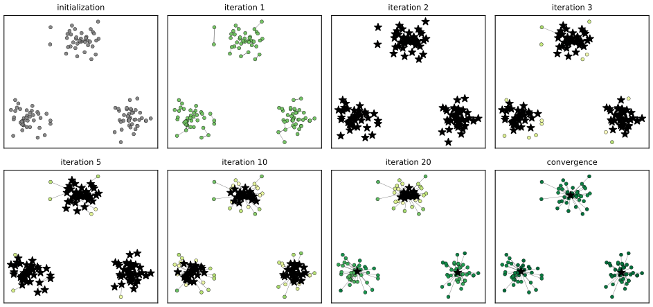
fig_9_17. Reproduces Murphy (2023), Figure 9.17. Download: PDF · SVG9.4.10 Emulating BP with graph neural nets
pp. 427–428 Message passing in PGMs uses fixed, model-independent update rules; graph neural networks (Section 16.3.6) learn the update from input-output pairs. Two uses are described: train a GNN on exact marginals of small PGMs and apply it to a similar one (Yoon et al., 2018), and deep unfolding (Hershey, Le Roux and Weninger, 2014), in which the \(T\) sweeps of BP on a fixed graph are unrolled into a \(T\)-layer network whose layers share the graph connectivity and whose parameters are then trained for a task. Both amortise inference: they pay off when the same graph and the same set of observed nodes are used many times.
9.5 The variable elimination (VE) algorithm
p. 428 Variable elimination computes a marginal \(p(z_Q\given y)\) exactly for any graph, with or without loops, discrete here (the Gaussian case uses the rules of Section 2.3.3). It is also called bucket elimination or peeling.
9.5.1 Derivation of the algorithm
pp. 428–430, (9.84)–(9.89), Figure 9.18, Tables 9.1–9.2 For the eight-variable student network (Coherence, Difficulty, Intelligence, Grade, SAT, Letter, Job, Happy) the marginal \(p(J)\) is a sum over seven variables of a product of eight factors, \(2^7\) terms by brute force (9.84). Pushing the sums inside the products gives, for the order \(C,D,I,H,G,S,L\), \[ p(J)=\sum_{L,S}\psi_J(J,L,S)\sum_G\psi_L(L,G)\sum_H\psi_H(H,G,J)\sum_I\psi_S(S,I)\psi_I(I)\sum_D\psi_G(G,I,D)\sum_C\psi_C(C)\psi_D(D,C). \] Working from the right (Table 9.1): \(\tau'_1(C,D)=\psi_C\psi_D\), \(\tau_1(D)=\sum_C\tau'_1\) (9.85)–(9.86); then \(\tau'_2(G,I,D)=\psi_G\tau_1\), \(\tau_2(G,I)=\sum_D\tau_2'\) (9.87)–(9.88), and so on until \(\tau_7(J)\). A conditional is a ratio of two such sums with the evidence clamped, e.g. \[ p(J=j\given I=1,H=0)=p(J=j,I=1,H=0)/\sum_{j'}p(J=j',I=1,H=0) \tag{9.89} \].
Result 9.16 (correctness of variable elimination) pp. 428–429
Let \(\Phi\) be a set of factors and \(p(x)\propto\prod_{\phi\in\Phi}\phi\). Eliminating \(x_1,\dots,x_n\) in turn, where at each step the factors that mention the variable are replaced by \(\tau=\sum_{x}\prod_{\phi\ni x}\phi\), leaves a factor equal to \(\sum_{x_1,\dots,x_n}\prod_{\phi\in\Phi}\phi\) (the unnormalised marginal of the remaining variables).
Proof
Distributivity: if the factors not involving \(x\) are \(\Phi_0\) and those that do are \(\Phi_x\), then \[ \sum_x\prod_{\Phi_0}\phi\prod_{\Phi_x}\phi=\prod_{\Phi_0}\phi\cdot\sum_x\prod_{\Phi_x}\phi \]. Hence replacing \(\Phi_x\) by \(\tau\) leaves the sum over the remaining variables unchanged; repeat \(n\) times. (The same argument works in any commutative semiring, supplement 9.2.3.) Evidence is handled by restricting each factor to the observed values (clamping) first.
In the code variable_elimination returns the trace of the product scopes. For the book's structure (with our own illustrative tables, see below) the scopes along \(C,D,I,H,G,S,L\) have sizes \(2,3,3,3,4,3,2\) and the largest created factor \(\tau\) has 3 variables; for the order \(G,I,S,L,H,C,D\) the first two \(\tau\) have scopes \((I,D,L,J,H)\) and \((D,L,S,J,H)\), exactly as in Table 9.2. Numbers. The book gives the structure of the network but no tables for \(J\) and \(H\); the code (and the demonstration) use our own tables (all variables binary, state 1 = high, hard, good, yes): \(p(C=1)=0.4\); \(p(D=1\given C=0,1)=0.3,0.6\); \(p(I=1)=0.3\); \(p(G=1\given D,I)\) for \((D,I)=(0,0),(0,1),(1,0),(1,1)\): \(0.6,0.9,0.3,0.7\); \(p(S=1\given I=0,1)=0.1,0.8\); \(p(L=1\given G=0,1)=0.1,0.8\); \(p(J=1\given L,S)=0.05,0.4,0.5,0.9\) for \((L,S)=(0,0),(0,1),(1,0),(1,1)\); \(p(H=1\given G,J)=0.2,0.6,0.5,0.95\) for \((G,J)=(0,0),(0,1),(1,0),(1,1)\). With them \(p(J=1)=0.4151\), obtained identically by both orders and by summing all 256 joint terms.
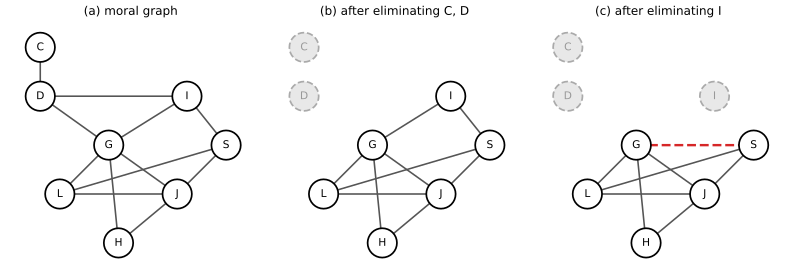
fig_9_18. Reproduces Murphy (2023), Figure 9.18. Download: PDF · SVG9.5.2 Computational complexity of VE
pp. 430–431, (9.90)–(9.92) The cost is dominated by the largest product \(\tau'\). Running VE symbolically (just tracking scopes) is the same as eliminating nodes from the graph, joining all remaining neighbours of the eliminated node by fill-in edges (Figure 9.18). Let \(G_{\prec}\) be the graph with all fill-in edges added for the order \(\prec\), the induced graph.
Result 9.17 (scopes are cliques of the induced graph; cost; chordality) pp. 430–431, (9.91)–(9.92)
(a) The scope of the product \(\tau'_i\) formed when \(v_i\) is eliminated is \(\{v_i\}\) together with the neighbours of \(v_i\) in the graph at that moment, and this set is a clique of \(G_\prec\). Every maximal clique of \(G_\prec\) is such a scope. (b) With all variables having \(K\) states the time is \(O(\sum_{c\in\mathcal C(G_\prec)}K^{|c|})\) over the maximal cliques (9.92), i.e. \(O(K^{w_\prec+1})\) times the number of cliques, with \(w_\prec=\max_c|c|-1\) the induced width. (c) \(G_\prec\) is chordal, and \(\prec\) is a perfect elimination ordering of it (no further fill-in). Conversely a graph has an elimination order with no fill-in iff it is chordal; trees and chordal graphs are exactly the graphs on which VE costs no more than the original factors.
Proof
(a) A factor mentions \(v_i\) at its elimination iff it is an original factor containing \(v_i\) or a \(\tau\) created earlier from a variable adjacent (in the current graph) to \(v_i\); by induction the union of scopes of these is \(v_i\) plus its current neighbours (original neighbours and those joined by earlier fill-in), and the algorithm adds fill-in edges that make this set a clique. (b) Forming \(\tau'_i\) takes \(K^{|C_i|}\) operations per scope \(C_i\); non-maximal scopes are contained in maximal ones, and we count only maximal cliques up to constants. (c) Let \(C=(u_1,\dots,u_k)\), \(k\ge4\), be a cycle of \(G_\prec\) and \(u\) its earliest eliminated vertex. At the time \(u\) is eliminated both its cycle neighbours are still present and are neighbours of \(u\), so the algorithm joins them: they are adjacent in \(G_\prec\), a chord of \(C\) (it is not an edge of the cycle because \(k\ge4\)). So every cycle of length at least 4 has a chord. The neighbours of \(v_i\) that come later in \(\prec\) form a clique by construction, which says exactly that \(\prec\) is a perfect elimination ordering of \(G_\prec\). Conversely a perfect elimination ordering of a graph yields no fill-in. (That every chordal graph has such an ordering is Dirac's theorem; a chordal graph has a vertex whose neighbours form a clique, a simplicial vertex, and removing it leaves a chordal graph.)
The code verifies the book's numbers (9.91)–(9.92): for the order \(C,D,I,H,G,S,L\) there is exactly one fill-in edge (G–S), the maximal cliques are \[ \{C,D\},\{D,I,G\},\{G,L,S,J\},\{G,J,H\},\{G,I,S\} \], the width is 3 and the cost is \(2^2+2^3+2^4+2^3+2^3=44\); for \(G,I,S,L,H,C,D\) there are nine fill-in edges, the maximal cliques are \(\{D,G,H,I,J,L\}\), \(\{D,H,I,J,L,S\}\), \(\{C,D\}\), the width is 5 and the cost 132. Adding the fill-in edges and re-running the elimination with the same order produces no new edges (chordality).
The treewidth of a graph is the smallest induced width over all orders. The \(\mathrm{arg\,min}\) of the cost over orders is NP-hard to find (Yannakakis, 1981; Arnborg et al., 1987), but with 8 nodes one can look at all \(8!=40{,}320\) orders. The student graph has treewidth 3 (also by an exact dynamic programme over subsets); 12,336 orders reach width 3, 16,704 width 4 and 11,280 width 5, the cost ranges from 44 (1,656 orders) to 192 (720 orders).
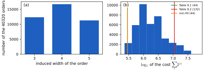
fig_9_S5. Download: PDF · SVG9.5.3 Picking a good elimination order
p. 432 The same numbers govern Cholesky factorisation of sparse matrices and einsum contraction orders. An ordering without fill-in is a perfect elimination ordering; decomposable graphs (trees, chordal graphs) have one. A common greedy heuristic is min-fill: eliminate any node with no fill-in, otherwise the node adding fewest fill-in edges (or min-weight for unequal state spaces). On the student graph it finds \(C,D,H,I,G,J,L,S\) (width 3, one fill-in edge, cost 44), the minimum over all 40,320 orders. Other methods in the book: simulated annealing, randomised approximations, nested dissection (METIS) and approximate minimum degree.
9.5.4 Computational complexity of exact inference
pp. 432–433, Figure 9.19 Variable elimination takes \(O(NK^{w+1})\) time, so inference is exponential in \(N\) for dense graphs. This is not a weakness of VE alone:
Filling the gap 9.6: exact inference is NP-hard, and #P-hard p. 433
Encode a 3-SAT formula with \(n\) variables \(Q_1,\dots,Q_n\) (independent fair coins) and \(m\) clauses as a Bayes net (Figure 9.19): a node \(C_t\) is the deterministic OR of the three literals of clause \(t\); nodes \(A_t\) form a chain of AND gates, \(A_2=C_1\wedge C_2\), \(A_t=A_{t-1}\wedge C_t\), so that the final node \(X\) is 1 iff all clauses are true (the chain keeps every conditional table of bounded size). Then \(p(X=1)=2^{-n}\cdot\#\{q:\text{all clauses true}\}\). Hence deciding whether \(p(X=1)>0\) decides satisfiability (NP-hard) and computing the normalising constant of the model with \(X\) clamped to 1 counts the satisfying assignments (#P-hard). Any marginal \(p(z\given X=1)\) needs this constant, so exact inference in general discrete graphical models is NP-hard (and #P-hard); approximating the marginals to within a relative error is also hard (Dagum and Luby 1993; Roth 1996). By contrast, finding one MAP assignment only needs one satisfying assignment, and is easier for some model classes. In the code a random formula with \(n=6\) variables and 9 clauses has 17 satisfying assignments out of 64; the Bayes net, solved by variable elimination with a min-fill order, gives \(p(X=1)=0.265625=17/64\) exactly.
With continuous hidden variables even a two-node model \(z\to y\) may be intractable to invert when the variables are high dimensional and not conjugate; so one resorts to the approximate methods of Chapters 10 and 11.
9.5.5 Drawbacks of VE
pp. 433–434, Figure 9.20 To get all marginals of a chain one would rerun VE for each \(z_t\): \(T\) times \(O(K^2T)\), i.e. \(O(K^2T^2)\), while forwards-backwards caches the messages and does it in \(O(K^2T)\). On a tree the same: the messages created while eliminating towards one root (the \(\tau\) factors) are reused when another node is the root. For a tree with \(n\) nodes, rooting at every node and sending \(n-1\) messages each would require \(n(n-1)\) messages, whereas two passes need only \(2(n-1)\) because each of the \(2(n-1)\) directed messages \(m_{s\to t}\) does not depend on the root. The remaining question is how to get this reuse when the graph is not a tree: the junction tree.
9.6 The junction tree algorithm (JTA)
p. 434 The JTA generalises variable elimination: run VE symbolically, add the fill-in edges (giving a chordal graph), convert it into a tree of cliques, and run belief propagation on that tree. The supplement (Chapter 9, Sections 9.1–9.2) spells this out; it is placed here. See also the companion course's outline (Algorithm 8.6).
Tree decompositions (supplement 9.2.1)
Supp. pp. 102–106, (S9.25)–(S9.27), Figures S9.2–S9.6 A tree decomposition of \(G=(V,E)\) is a tree \(T\) whose nodes \(t\) carry "meganodes" \(X_t\subseteq V\) such that (i) \(\bigcup_tX_t=V\); (ii) every edge \((u,v)\in E\) lies in some \(X_t\); (iii) for each \(v\), \(\{t:v\in X_t\}\) is a subtree of \(T\) (equivalently the running intersection property: \(X_i\cap X_j\subseteq X_k\) for every \(X_k\) on the path between them). Its width is \(\max_t|X_t|\) and the treewidth of \(G\) is the minimum width over decompositions, minus one, (S9.26). A tree has treewidth 1.
Why. In a tree any single node separates the graph into two parts, which supports dynamic programming over the separators. Computing one. Triangulation: eliminate nodes in an order \(\pi\) (see 9.5.3), form the clique \(C_i=\{v_i\}\cup(\text{uneliminated neighbours})\) with fill-in edges; the result is chordal; keep the maximal cliques (drop \(C_i\) if contained in an earlier one); connect them: the junction graph has an edge between cliques with a non-empty intersection, weighted by \(|C_i\cap C_j|\), and any maximum-weight spanning tree of it is a junction tree (Jensen and Jensen, 1994; Aji and McEliece, 2000).
Result 9.18 (an elimination order gives a tree decomposition of width \(w_\prec+1\); treewidth equals the minimum induced width) Supp. pp. 102–105
For any elimination order \(\prec\), take bags \(X_i=C_i\) (the elimination cliques) and join \(i\) to the bag of the first eliminated vertex among \(C_i\setminus\{v_i\}\). This is a tree decomposition of \(G\) of width \(\max_i|C_i|=w_\prec+1\). Conversely every tree decomposition of width \(k\) comes from an order with induced width \(k-1\); hence \(\mathrm{tw}(G)=\min_\prec w_\prec\).
Proof (the construction direction)
Properties (i)–(ii): each \(v_i\in C_i\); an edge \((u,v)\) with \(u\) eliminated first lies in \(C_u\). Tree: each \(C_i\) except the last has a parent (a later-eliminated bag), so there is no cycle and, rooted at the last bag, it is a tree. Property (iii): let \(v\) be a vertex and \(i\) the bag in which \(v\) is eliminated; \(v\in C_j\) with \(j\ne i\) means \(v\) is a neighbour of \(v_j\) when \(v_j\) is eliminated, and then \(v\) is a (later) member of \(C_j\setminus\{v_j\}\), so the parent of \(j\) is the bag of the earliest such member \(v_{j'}\), and \(v\in C_{j'}\) because \(v\) is a neighbour of \(v_j\) and the neighbours of \(v_j\) become a clique before \(v_{j'}\) is eliminated (they are joined by fill-in). Following parents from \(j\) we stay inside bags containing \(v\) until we reach \(i\); hence the bags containing \(v\) form a connected subtree. The converse (every decomposition yields an order, by eliminating the bag-private vertices leaf to root) is classical (Bodlaender, 1993); the code checks \(\mathrm{tw}=\min_\prec w_\prec\) on the student graph by exhaustive search over 40,320 orders (3) and by an independent exact dynamic programme (3), and for grids, \(3\times3\), \(3\times4\), \(4\times4\), \(2\times6\) (3, 3, 4, 2).
Common structures Supp. p. 105, Figures S9.5–S9.6: a chain has treewidth 1 and can trade \(O(T)\) memory for \(O(\log T)\) at runtime \(O(T\log T)\) by checkpointing; a \(w\times h\) grid has treewidth \(\min(w,h)\) (group each column or row into one meganode; the lower bound is due to Lipton and Tarjan). The code finds exactly \(\min(w,h)\) for the small grids above, and that eliminating column by column along the long side of a \(5\times7\) grid gives width 5. A graph can look triangulated and not be: the graph of Supplementary Figure 9.6(a) is made of little triangles but contains the chordless 5-cycle 1-2-3-4-5-1 and needs two fill-in edges. (Our check of the pure 5-cycle: eliminating it in cyclic order creates 2 fill-in edges and three triangles, width 2, cost \(3K^3\); see Problem 9.3.)
Result 9.19 (junction trees are the maximum-weight spanning trees of the junction graph) Supp. p. 105
Let \(\mathcal C\) be the maximal cliques of a chordal graph. For a tree \(T\) on \(\mathcal C\) put \(w(T)=\sum_{(i,j)\in T}|C_i\cap C_j|\) and \(n_v=\#\{C\in\mathcal C:v\in C\}\). Then \(w(T)\le\sum_v(n_v-1)\) with equality iff \(T\) has the running intersection property. Since a junction tree exists for a chordal graph, the maximum-weight spanning trees are exactly the junction trees.
Proof
\(w(T)=\sum_v\#\{(i,j)\in T:v\in C_i\cap C_j\}\). For a fixed \(v\), the edges of \(T\) whose both ends contain \(v\) form a forest on the \(n_v\) cliques that contain \(v\) (a subgraph of a tree), so there are at most \(n_v-1\) of them, with equality iff that forest is connected, i.e. the cliques containing \(v\) form a subtree. Summing over \(v\) gives the inequality, and equality iff the condition holds for every \(v\), which is the running intersection property. The existence of a tree attaining it for chordal graphs follows from the elimination construction of Result 9.18; every maximum-weight spanning tree then attains the same maximum and hence has the property. The code checks the identity for the student graph (weight \(7=\sum_v(n_v-1)\)) and shows the failure for the four cliques of a 4-cycle: the best spanning tree violates the property.
For the student network, moralised, with the order \(C,D,I,H,G,S,L\) (and \(J\) last), the maximal cliques of the chordal graph are \[ \{C,D\},\{G,I,D\},\{G,S,I\},\{G,J,S,L\},\{H,G,J\} \tag{S9.27} \]; the junction tree is the path \(CD-DGI-GIS-GJLS-GHJ\) with separators \(D,GI,GS,GJ\).
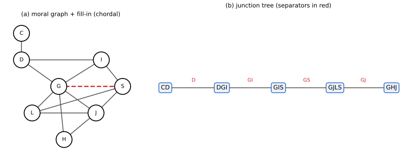
fig_S9_4. Reproduces Murphy (2023), Supplementary Figure 9.4. Download: PDF · SVGMessage passing on a junction tree (supplement 9.2.2)
Supp. pp. 106–109, (S9.28)–(S9.37), Figure S9.7 This is the Lauritzen–Spiegelhalter algorithm. Each clique \(i\) carries a potential \(\phi_i\) (a non-negative table on \(C_i\)) and each tree edge a separator potential \(\phi_{ij}\) on \(S_{ij}=C_i\cap C_j\). Operations: marginalise \(\phi_{ij}(S_{ij})=\sum_{C_i\setminus S_{ij}}\phi_i\) (S9.28); multiply \((\phi_j*\phi_{ij})(C_j)=\phi_j\phi_{ij}\) by broadcasting (S9.29); divide \(\phi_j/\phi_{ij}\) with \(0/0=0\) (S9.30). Initialisation: assign each factor \(F_k\) to one clique containing its variables, \(\phi_i=\prod_{k\to i}F_k\) (identity 1 if none), and \(\phi_{ij}=1\) (S9.31). Calibration: pick a root; collect in post-order, each node \(n\) sends to its parent \(p\): \(\phi_{np}\leftarrow\sum_{C_n\setminus S}\phi_n\), \(\phi_p\leftarrow\phi_p*\phi_{np}\) (S9.33–S9.34); distribute in pre-order, each child \(c\) of \(n\) first divides out the old separator and multiplies in the new: \(\phi_{nc}^{new}=\sum_{C_n\setminus S}\phi_n\), \(\phi_c\leftarrow\phi_c*\phi_{nc}^{new}/\phi_{nc}^{old}\) (S9.35–S9.37).
Result 9.20 (calibration gives the clique and separator marginals) Supp. pp. 106–109
Let \(\tilde p(x)=\prod_kF_k(x)\). Throughout the algorithm \(\prod_i\phi_i/\prod_{(ij)}\phi_{ij}=\tilde p\) (the invariant). After the collect pass the root potential is the unnormalised marginal of \(\tilde p\) on its clique; after the distribute pass every \(\phi_i\) is \(\sum_{x\setminus C_i}\tilde p\) and every \(\phi_{ij}\) is \(\sum_{x\setminus S_{ij}}\tilde p\). So all clique marginals are obtained with two messages per edge, and the normaliser \(\sum_{C_i}\phi_i=Z\) is the same at every clique.
Proof
Invariant. An absorption from \(i\) to \(j\) replaces \(\phi_{ij}\) by \(\phi'_{ij}=\sum\phi_i\) and \(\phi_j\) by \(\phi_j\phi'_{ij}/\phi_{ij}\). The product \(\phi_j/\phi_{ij}\) becomes \(\phi_j\phi'_{ij}/\phi_{ij}/\phi'_{ij}=\phi_j/\phi_{ij}\): unchanged. (Initially \(\phi_{ij}=1\) and \(\prod_i\phi_i=\prod_kF_k\).)
Collect. Let \(F_{(c)}\) be the product of original factors assigned to the cliques of the subtree below \(c\) (including \(c\)). By induction, after the children of \(c\) have sent, \[ \phi_c=\sum_{x_{\text{below}}\setminus C_c}F_{(c)}=:G_c(C_c) \] (a clique potential multiplied by the messages of its children, each a sum over a subtree) and the message to its parent is \(\phi_{cp}=\sum_{C_c\setminus S}G_c=:\varphi_c(S)\). At the root \(\phi_{root}\) is the sum of \(\tilde p\) over everything except the root clique.
Distribute. Suppose \(\phi_p=\sum_{x\setminus C_p}\tilde p\) is already the marginal. For its child \(c\) with separator \(S\), the new separator is \[ \phi^{new}_{pc}(S)=\sum_{x\setminus S}\tilde p=\varphi_c(S)\psi_{rest}(S) \], where \(\psi_{rest}(S)\) is the sum of the product of all factors outside the subtree of \(c\) (by the running intersection property the two parts interact only through \(S\), so the sum factorises). After the update \[ \phi_c=G_c(C_c)\cdot\frac{\varphi_c(S)\psi_{rest}(S)}{\varphi_c(S)}=G_c(C_c)\psi_{rest}(S)=\sum_{x\setminus C_c}F_{(c)}F_{rest}=\sum_{x\setminus C_c}\tilde p, \] again because \(F_{rest}\) depends on \(x_{C_c}\) only through \(S\). Induct down the tree. The code runs this algorithm (with division) on the student network: all five clique potentials and the four separator potentials equal the marginals of the enumerated joint to \(10^{-12}\), and the normaliser is 1.
The Shafer–Shenoy variant avoids division by keeping the individual incoming messages and multiplying all but one on demand (like (9.60) against (9.61)).
The generalized distributive law (supplement 9.2.3)
Supp. pp. 109–110, (S9.38)–(S9.40), Table S9.1 For a four-step chain \[ Z=\sum_{x_1}\dots\sum_{x_4}\psi_{12}\psi_{23}\psi_{34}=\sum_{x_1}\sum_{x_2}\psi_{12}\sum_{x_3}\psi_{23}\sum_{x_4}\psi_{34} \tag{S9.38, S9.39} \]. The same pushing-in works whenever the local functions take values in a commutative semiring \((K,+,\times)\): \(+\) and \(\times\) associative and commutative with identities 0 and 1, and the distributive law \((a\times b)+(a\times c)=a\times(b+c)\) (S9.40).
| Domain | \(+\) | \(\times\) | Problem |
|---|---|---|---|
| \([0,\infty)\) | (sum, 0) | (product, 1) | sum-product (marginals, \(Z\)) |
| \([0,\infty)\) | (max, 0) | (product, 1) | max-product (MAP) |
| \((-\infty,\infty]\) | (min, \(\infty\)) | (sum, 0) | min-sum (energies) |
| \(\{T,F\}\) | (\(\vee\), F) | (\(\wedge\), T) | satisfiability |
Result 9.21 (the generalised distributive law) Supp. pp. 109–110
Everything in this chapter that uses only sums, products, distributivity and the existence of identities (VE, tree and junction tree message passing) is valid for any commutative semiring, with "sum" replaced by \(+\) and "product" by \(\times\). Division (as in the Lauritzen–Spiegelhalter version) additionally requires inverses, which exist for sum-product and min-sum (as subtraction) but not for max-product, so there one uses the Shafer–Shenoy form.
Proof
The correctness proofs of Result 9.16 and Result 9.8 use only (i) \(\sum_x a\,f(x)=a\sum_xf(x)\) when \(a\) does not depend on \(x\) (the distributive law) and (ii) associativity and commutativity to reorder sums and products. Both hold in a semiring. Max-product: \(\max_x(af(x))=a\max_xf(x)\) for \(a\ge0\), so \((\max,\times)\) on \([0,\infty)\) is a semiring; min-sum is the same structure after \(x\mapsto-\log x\) (\(\min(a+f)=a+\min f\)). In the code the four semirings are compared on a random 4-step chain: the pushed-in sum equals the brute-force sum (sum-product), the pushed-in maximum equals the brute-force maximum (max-product), the min-sum value equals \(-\log\) of the max-product value, and the Boolean version agrees on satisfiability.
Uses listed in the supplement: posterior marginals and samples (Dawid), the \(N\) most probable assignments (Nilsson), constraint satisfaction, logical reasoning, and solving sparse linear systems \(Ax=b\) (via Gaussian BP).
JTA applied to a chain (supplement 9.2.4)
Supp. pp. 110–111, (S9.41)–(S9.47), Figure S9.8 For an HMM the cliques are the edges of the backbone, \((X_{t-1},X_t)\), and the leaves \((X_t,Y_t)\); separators are the single nodes. Initialise \(\phi_{(X_{t-1},X_t)}=A\), \(\phi_{(X_t,Y_t)}=p(y_t\given X_t)\), separators 1. On the forward pass, the clique \(j=(X_{t-1},X_t)\) receives from its left neighbour the marginal on \(X_{t-1}\), which is \(\alpha_{t-1}\) (the filtered belief), and from the leaf the evidence \(\lambda_t(X_t)\); absorbing both gives \[ \phi^*_j(X_{t-1},X_t)\propto A(X_{t-1},X_t)\,\alpha_{t-1}(X_{t-1})\,\lambda_t(X_t)\propto p(X_{t-1},X_t\given y_{1:t}), \] the filtered two-slice marginal (S9.44). On the backward pass the right neighbour sends the separator \(\gamma_t(X_t)\) and divides by the old one \(\alpha_t(X_t)\): \[ \phi^{**}_j\propto[A\,\alpha_{t-1}\lambda_t]\gamma_t(X_t)/\alpha_t(X_t)\propto p(X_{t-1},X_t\given y_{1:T}) \] (S9.45–S9.47), which is the smoothed two-slice marginal (9.35) of Result 9.4. Thus the junction tree algorithm on a chain is forwards filtering, backwards smoothing. (In the supplement the indices of (S9.41)–(S9.43) are inconsistent, with "\(\alpha_{t-1})(X_t)\)" and the clique names \(i,j\) reused; the form above is the consistent one.) The code verifies on a 3-state, 4-step HMM that the calibrated clique potentials are the two-slice marginals \(\xi_{t,t+1}\) of forwards-backwards and that the normaliser is \(p(y_{1:T})\) (difference \(10^{-17}\)).
JTA for general temporal graphical models (supplement 9.2.5)
Supp. pp. 111–113, (S9.48)–(S9.49), Figure S9.9 A dynamic Bayes net with \(M\) hidden chains of \(K\) states per time slice can be flattened into one chain with \(K^M\) states whose transition matrix is the Kronecker product of the chain matrices; two independent chains with \(A_1=\begin{pmatrix}a&b\\c&d\end{pmatrix}\), \(A_2=\begin{pmatrix}e&f\\g&h\end{pmatrix}\) give \(A=A_1\otimes A_2\), with entry \((1,2)\to(2,1)\) equal to \(b\,g\), and the matrix is dense even though the chains are independent. Forwards-backwards on it costs \(O(TK^{2M})\). The JTA gives \(O(TMK^{M+1})\): update the belief state one variable at a time while sweeping a "frontier" of cliques across the network (the frontier algorithm of Zweig and Russell), because the hidden variables of a slice are made dependent by a common observed child (explaining away), so the exact belief state has size \(K^M\) but the transition can be applied variable by variable. The exact belief state is necessarily exponential in \(M\): in a coupled HMM, after \(T=M\) steps influence has travelled between all chains ("entanglement"), so the belief state is fully correlated. This is why one uses structured mean field (\(O(TMK^2I)\) for \(I\) iterations, Section 10.3.2) or assumed density filtering. For linear dynamical systems things are better: combining chains increases the state dimension additively, so inference costs \(O(T(CL)^3)\) for \(C\) chains of dimension \(L\), and independent chains give a block-diagonal rather than a Kronecker-product matrix. The code verifies the Kronecker entry and that the filter of the flattened chain of two independent chains (with a product likelihood) is the product of the two separate filters.
The supplement's Figures S9.2–S9.3 and S9.6 (the junction tree of the small graph, the triangulation steps) are small graph drawings; the student-network triangulation (Figure S9.4) is reproduced above.
9.7 Inference as optimization
p. 435 Inference can be posed as an optimisation problem, often simpler computationally (see also the supplement's Section 9.3).
9.7.1 Inference as backpropagation
pp. 435–436, (9.93)–(9.95), Listing 9.1 Write a pairwise discrete model as an exponential family, \(p(x)=\exp(\eta^\T T(x)-A(\eta))\) (9.93), with the sufficient statistics the node and edge indicators, \(T(x)=(\{\mathbb 1(x_s=j)\},\{\mathbb 1(x_s=j,x_t=k)\})\), natural parameters the log potentials \(\eta=(\{\log\psi_s(j)\},\{\log\psi_{st}(j,k)\})\) and \(A(\eta)=\log Z(\eta)\). The mean parameters are \[ \mu=\mathbb E[T(x)]=(\{p(x_s=j)\},\{p(x_s=j,x_t=k)\}) \tag{9.94} \].
Result 9.22 (marginals are the gradient of the log partition function) p. 435, (9.94)
\(\mu=\nabla_\eta\log Z(\eta)\): \(\partial\log Z/\partial\log\psi_s(j)=p(x_s=j)\) and \(\partial\log Z/\partial\log\psi_{st}(j,k)=p(x_s=j,x_t=k)\). If some variables are clamped to observed values by multiplying one-hot vectors into the node potentials, the same gradient gives the marginals conditional on the evidence.
Proof
\(Z(\eta)=\sum_x\exp(\eta^\T T(x))\), so \(\partial Z/\partial\eta_i=\sum_xT_i(x)\exp(\eta^\T T(x))\) and \(\partial\log Z/\partial\eta_i=\mathbb E[T_i(x)]\) (this is Equation (2.236), Chapter 2). With indicator statistics, the expectation of an indicator is the corresponding probability. For evidence \(x_t=e\), multiply \(\psi_t\) by \(\mathbb 1(x_t=e)\) (equivalently set the other log-potentials to \(-\infty\)): \(Z_e=\sum_{x:x_t=e}\tilde p(x)\), and the gradient is the expectation under \(\tilde p(x)\mathbb 1(x_t=e)/Z_e=p(x\given x_t=e)\).
For the chain \(x_1-x_2-x_3\) the partition function is \(Z=\sum\psi_1\psi_2\psi_3\psi_{12}\psi_{23}\) (9.95), computed by einsum and differentiated by automatic differentiation: in two lines of code. The book's listing is in JAX; the code of this course does the same with PyTorch (autodiff_marginals), and we confirm that \(\log Z\) equals the log of the enumerated normaliser and that the gradients are the node marginals and the pairwise marginals to \(10^{-12}\), and (with \(x_3\) clamped) the conditional marginals. (In the book's listing the logarithm is written np.log; inside a JAX-differentiated function it must be jnp.log. We did not run JAX, so treat this as a note, not a confirmed error.)
Filling the gap 9.7: backpropagation is the backwards pass p. 435
The book does not say why reverse-mode differentiation costs only a small multiple of computing \(Z\). For an HMM, \[ Z=p(y_{1:T})=\mathbf 1^\T D_T\mathbf A^\T D_{T-1}\cdots\mathbf A^\T D_1\pi \] with \(D_t=\mathrm{diag}(\lambda_t)\). Write \(Z=\sum_j\alpha'_t(j)\beta'_t(j)\) with \(\alpha'_t(j)=p(z_t=j,y_{1:t})\) (contains \(\lambda_t(j)\) as a factor) and \(\beta'_t(j)=p(y_{t+1:T}\given z_t=j)\). Then \[ \partial Z/\partial\lambda_t(j)=\alpha'_t(j)\beta'_t(j)/\lambda_t(j) \], so \[ \frac{\partial\log Z}{\partial\log\lambda_t(j)}=\frac{\alpha'_t(j)\beta'_t(j)}{Z}=\gamma_t(j). \] The adjoint (gradient) variables propagated backwards by reverse-mode differentiation through the forward recursion are exactly the \(\beta'\) messages, and the total cost of the gradient is the cost of the forward and backward passes, \(O(K^2T)\). The same holds on trees and, with the junction tree for \(Z\), in general. The code checks \(\partial\log p(y)/\partial\log\lambda_t(j)=\gamma_t(j)\) by autodiff through the forwards algorithm (difference \(10^{-10}\)). This is Eisner's observation that "inside-outside" is backpropagation, and gives differentiable inference layers.
9.7.2 Perturb and MAP
pp. 436–437 To sample from a model by solving optimisation problems: make \(S\) copies with perturbed parameters \(\tilde\theta_s=\theta+\epsilon_s\) and take \(x_s=\mathrm{arg\,max}\,p(x\given y;\tilde\theta_s)\). For well-chosen noise this gives exact samples (Papandreou and Yuille, 2010, 2011).
Gaussian case
(9.96)–(9.104) Let the prior be \(p(x)\propto\mathcal N(Gx\given\mu_p,\Sigma_p)\) and the likelihood \(p(y\given x)=\mathcal N(y\given Hx+c,\Sigma_n)\). The posterior is \(\mathcal N(\mu,K^{-1})\) with \[ K=G^\T\Sigma_p^{-1}G+H^\T\Sigma_n^{-1}H,\qquad \mu=K^{-1}(G^\T\Sigma_p^{-1}\mu_p+H^\T\Sigma_n^{-1}(y-c)). \tag{9.99, 9.100} \]
Result 9.23 (perturb-and-MAP is exact for Gaussians; the Gumbel-max trick for discrete models) pp. 436–437, (9.102)–(9.104)
(a) Draw \(\epsilon_\mu\sim\mathcal N(0,\Sigma_p)\), \(\epsilon_y\sim\mathcal N(0,\Sigma_n)\) independently and let \[ \tilde x=K^{-1}(G^\T\Sigma_p^{-1}(\mu_p+\epsilon_\mu)+H^\T\Sigma_n^{-1}(y+\epsilon_y-c)) \], the MAP of the perturbed problem. Then \(\tilde x\sim\mathcal N(\mu,K^{-1})\). (b) For a finite state space, if \(\epsilon_x\) are i.i.d. standard Gumbel, \(\Pr[\mathrm{arg\,max}_x(\log p(x)+\epsilon_x)=x_0]=p(x_0)\).
Proof
(a) \(\tilde x=\mu+A\epsilon_\mu+B\epsilon_y\) with \(A=K^{-1}G^\T\Sigma_p^{-1}\), \(B=K^{-1}H^\T\Sigma_n^{-1}\) (9.104): linear in Gaussian noise, so Gaussian with mean \(\mu\) and covariance \[ A\Sigma_pA^\T+B\Sigma_nB^\T=K^{-1}(G^\T\Sigma_p^{-1}G+H^\T\Sigma_n^{-1}H)K^{-1}=K^{-1}. \] (b) Let \(U_x=\log p(x)+\epsilon_x\); \(\Pr[\epsilon\le s]=e^{-e^{-s}}\), so \(\Pr[U_x\le u]=\exp(-p(x)e^{-u})\). Conditioning on \(U_{x_0}=u\) (density \(p(x_0)e^{-u}\exp(-p(x_0)e^{-u})\)) the probability that all others are smaller is \[ \prod_{x\ne x_0}\exp(-p(x)e^{-u})=\exp(-(1-p(x_0))e^{-u}) \], so \[ \Pr[x_0\text{ wins}]=\int p(x_0)e^{-u}\exp(-e^{-u})\,du=p(x_0)\int_0^\infty e^{-v}dv=p(x_0) \] (substituting \(v=e^{-u}\)). The code draws 200,000 Gaussian samples (five-dimensional posterior, three measurements): the sample mean and covariance agree with \(\mu\) and \(K^{-1}\) to \(0.002\) and \(0.003\), and the Gumbel-max sampler for a 64-state ring Ising model has total variation distance \(0.0044\) to \(p\) (the level of Monte Carlo noise).
The Gaussian method is very scalable because the MAP of a sparse GMRF is a sparse linear system (conjugate gradient, or Gaussian BP: Result 9.14 shows that BP gives the exact mean whenever it converges).
Discrete case
p. 437, (9.105) The score is \[ S(x;c)=\sum_i\log\phi_i(x_i)+\sum_{ij}\log\psi_{ij}(x_i,x_j) \]. The exact sampler would put Gumbel noise on every configuration (exponentially many), which defeats the purpose; the practical approximation perturbs only the local evidence terms, \(\log\phi_i(k)+\epsilon_{ik}\), and solves the MAP with an efficient solver (for example the graph cuts of the supplement). The approximation is not exact: for a ring of six binary variables with random fields and coupling 0.8, Gumbel noise on the unary terms only gives a distribution with total variation distance 0.23 from \(p\), against 0.01 for the exact version (Figure 9.S4). It is nevertheless useful for learning and for estimating partition functions (Hazan and Jaakkola 2012).
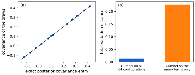
fig_9_S4. Download: PDF · SVGMAP estimation for discrete PGMs (supplement 9.3)
Supp. pp. 113–121 Here the aim is the MAP assignment \(x^*=\mathrm{arg\,max}_{x\in\mathcal X^V}p(x)\) of a pairwise MRF \[ p(x)=Z^{-1}\exp\{\sum_s\theta_s(x_s)+\sum_{(s,t)\in E}\theta_{st}(x_s,x_t)\} \tag{S9.50} \], which can ignore \(Z\): \[ x^*=\mathrm{arg\,max}_x\sum_s\theta_s(x_s)+\sum_{(s,t)}\theta_{st}(x_s,x_t) \tag{S9.52} \]. Dynamic programming (Section 9.2) is exact but exponential in the treewidth, so for intractable models one needs approximations. (The supplement's \(x_s\) and \(x\) correspond to the chapter's \(z\).)
Notation (supplement 9.3.1)
Supp. pp. 113–114, (S9.53)–(S9.57) Write \(p(x)=Z(\theta)^{-1}\exp(-E(x))\), \(E(x)=-\theta^\T T(x)\), where the canonical parameters are \(\theta=(\{\theta_{s;j}\},\{\theta_{st;jk}\})\) and \(T(x)=(\{\mathbb 1(x_s=j)\},\{\mathbb 1(x_s=j,x_t=k)\})\). The mean parameters \(\mu=\mathbb E[T(x)]=(\{\mu_{s;j}\},\{\mu_{st;jk}\})\) are single and pairwise marginals, a vector of length \(d=KV+K^2E\) (the standard overcomplete representation, because it ignores the sum-to-one constraints). For binary \(x_s\in\{0,1\}\) a minimal representation uses \(T=(x_s,x_sx_t)\) of dimension \(d=V+E\) with \(\mu_s=p(x_s=1)\) and \(\mu_{st}=p(x_s=x_t=1)\).
The marginal polytope (supplement 9.3.2)
Supp. p. 114–115, (S9.58)–(S9.61), Figure S9.10 The marginal polytope is the set of realisable mean parameters, \[ \mathcal M(G)=\{\mu:\exists p\ge0,\ \sum_xp(x)=1,\ \mu=\sum_xT(x)p(x)\}=\mathrm{conv}\{T(x):x\in\mathcal X^V\} \tag{S9.58, S9.60} \].
Filling the gap 9.8: the four inequalities for two binary nodes Supp. p. 114, (S9.59)–(S9.61)
For \(x_1-x_2\) with binary states, \[ \mu=(\mu_1,\mu_2,\mu_{12})=(\Pr[x_1=1],\Pr[x_2=1],\Pr[x_1=x_2=1]) \]. Every realisable \(\mu\) satisfies \(\mu_{12}\ge0\), \(\mu_{12}\le\mu_1\), \(\mu_{12}\le\mu_2\) (a joint probability is at most each marginal) and \(1-\mu_1-\mu_2+\mu_{12}=\Pr[x_1=x_2=0]\ge0\). Conversely the four vertices \(T(x)\) are \((0,0,0)\), \((1,0,0)\), \((0,1,0)\), \((1,1,1)\), forming a tetrahedron with four faces, and the four faces are exactly the planes \(\mu_{12}=0\), \(\mu_{12}=\mu_1\), \(\mu_{12}=\mu_2\), \(\mu_1+\mu_2-\mu_{12}=1\) (each contains three of the four vertices: for example the plane \(\mu_{12}=0\) contains \((0,0,0),(1,0,0),(0,1,0)\)). So the polytope described by the four inequalities, written \(A\mu\le b\) with \[ A=\begin{pmatrix}0&0&-1\\-1&0&1\\0&-1&1\\1&1&-1\end{pmatrix} \], \(b=(0,0,0,1)^\T\), equals the convex hull \(\mathrm{conv}\{(0,0,0),(1,0,0),(0,1,0),(1,1,1)\}\) (S9.61). (The printed matrix form (S9.59) lists \(-1\) in each row; the code checks the hull against the inequalities on 4,000 random points and they agree, with volume fraction 1/6, the volume of the tetrahedron.)
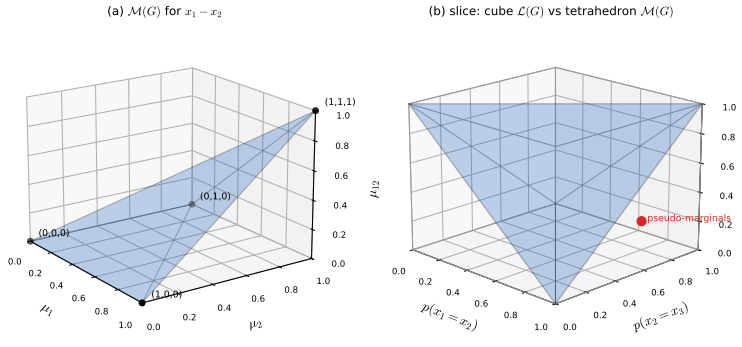
fig_S9_10. Reproduces Murphy (2023), Supplementary Figures 9.10(a) and 9.11(b). Download: PDF · SVGLinear programming relaxation (supplement 9.3.3)
Supp. pp. 115–117, (S9.62)–(S9.67), Figure S9.11 Local consistency: \(\sum_{x_s}\tau_s(x_s)=1\) (S9.64) and \(\sum_{x_t}\tau_{st}(x_s,x_t)=\tau_s(x_s)\) (S9.65) for every edge (in both directions), and \(\tau\ge0\). The set of such \(\tau\) is the local polytope \(\mathcal L(G)\) (S9.66); its elements are pseudo-marginals.
Result 9.24 (MAP is a linear program over the marginal polytope; its relaxation over \(\mathcal L(G)\); exactness on trees) Supp. pp. 115–116
(a) \[ \max_x\theta^\T T(x)=\max_{\mu\in\mathcal M(G)}\theta^\T\mu \tag{S9.62} \]. (b) \(\mathcal M(G)\subseteq\mathcal L(G)\), with equality iff \(G\) is a tree (for the "if" direction; for graphs with loops the inclusion is strict, in the standard overcomplete representation). Hence \[ \max_{\tau\in\mathcal L(G)}\theta^\T\tau\ge\max_x\theta^\T T(x) \tag{S9.63} \], with equality, and an integral \(\tau^*\), for a tree.
Proof
(a) A linear function on the convex hull of finitely many points attains its maximum at one of the points, the vertices \(T(x)\) are the extreme points, and \(\theta^\T T(x)\) at the maximiser \(x^*\) is the value; the other inequality is trivial since \(T(x)\in\mathcal M\). Non-degenerate ("soft") \(\mu\) are not vertices, so they cannot do strictly better. (b) Any realisable \(\mu\) satisfies normalisation and marginalisation, so \(\mathcal M\subseteq\mathcal L\). For a tree \(T\) and \(\tau\in\mathcal L(T)\) define \[ p_\tau(x)=\prod_s\tau_s(x_s)\prod_{(s,t)}\tau_{st}(x_s,x_t)/(\tau_s(x_s)\tau_t(x_t)) \tag{S9.67} \]. Induction on the number of nodes: removing a leaf \(\ell\) with neighbour \(m\) leaves a tree for which \(p_\tau\) restricted has, by the induction hypothesis, marginals \(\tau\); \(p_\tau\) equals the smaller product times \(\tau_{\ell m}(x_\ell,x_m)/\tau_m(x_m)\), and summing over \(x_\ell\) gives \(\tau_m/\tau_m=1\) by marginalisation consistency, so \(p_\tau\) is a distribution with single node marginals \(\tau_s\) and edge marginals \(\tau_{st}\) (this is Result 9.7 read backwards). So \(\tau\in\mathcal M(T)\). The code checks this on 10 random tree-structured joint distributions: the product (S9.67) built from their node and edge marginals is normalised and has those marginals, and in the LP check below all 10 random 6-node trees with 3 states give an integral optimum equal to the MAP value (error \(10^{-7}\)).
Filling the gap 9.9: the pseudo-marginals of Figure S9.11 are not marginals of any distribution; a frustrated triangle Supp. pp. 116–117
The supplement's example has three binary nodes on a triangle with uniform node marginals and edge marginals implying \(p(x_1=x_2)=0.8\), \(p(x_2=x_3)=0.8\), \(p(x_1=x_3)=0.2\). Each is locally consistent, so the point lies in \(\mathcal L(G)\). It cannot be in \(\mathcal M(G)\): for any joint distribution, if \(x_1=x_2\) and \(x_2=x_3\) then \(x_1=x_3\), so \[ \mathbb 1[x_1=x_2]+\mathbb 1[x_2=x_3]-\mathbb 1[x_1=x_3]\le1 \] pointwise, and taking expectations \(0.8+0.8-0.2=1.4\le1\) is violated. (These cycle inequalities are facets of the marginal polytope of the triangle, giving the tetrahedron in the figure.) The code confirms by linear programming that no joint distribution on the 8 states has these edge marginals, while with \(p(x_1=x_3)=0.8\) there is one. The same triangle gives an LP relaxation that is not tight: with the reward \(\theta_{st}(x_s,x_t)=\mathbb 1[x_s\ne x_t]\) on all three edges, the best assignment can disagree on at most two edges (MAP value 2) but the LP optimum is 3, attained by the fractional \(\tau_s=(\tfrac12,\tfrac12)\), \(\tau_{st}(0,1)=\tau_{st}(1,0)=\tfrac12\). On 10 random loopy graphs on 5 nodes the LP value is never below the MAP value. In practice the fractional solution is rounded (Werner 2007).
Supp. pp. 115–117 Algorithms. A generic LP solver works but is slow; message-passing methods exist for the same relaxation (tree-reweighted BP, Chapter 10), and the supplement then shows an application of BP to stereo depth estimation (Figure S9.12: the Venus images with Gaussian and robust edge potentials). The figure needs the Middlebury stereo pair, which is not available to us; it is skipped.
Graphcuts (supplement 9.3.4)
Supp. pp. 118–120, (S9.68)–(S9.71), Figures S9.13–S9.15 For binary MRFs with Ising pairwise energies \(E_{uv}(x_u,x_v)=0\) if \(x_u=x_v\), \(\lambda_{uv}\ge0\) if \(x_u\ne x_v\) (S9.68), the MAP (minimum-energy) state is a minimum cut. Shift each unary energy so that \(E_u(1)=0\) or \(E_u(0)=0\); add a source \(s\), a sink \(t\); if \(E_u(1)=0\) add the edge \(x_u\to t\) with capacity \(E_u(0)\); if \(E_u(0)=0\) add \(s\to x_u\) with capacity \(E_u(1)\); for every MRF edge add \(x_u\to x_v\) and \(x_v\to x_u\) with capacity \(\lambda_{uv}\). A minimum \(s\)-\(t\) cut splits the nodes into \(X_s\ni s\) and \(X_t\ni t\); nodes in \(X_s\) take state 0 and nodes in \(X_t\) state 1.
Result 9.25 (graph cuts give the exact MAP of submodular binary MRFs; \(\alpha\)-expansion needs a metric) Supp. pp. 118–120
(a) Under the construction above the cost of a cut equals the energy of the corresponding labelling. (b) For general pairwise energies a labelling's energy can be written as unary terms plus \(\sum_{(u,v)}\kappa_{uv}\mathbb 1[x_u=0,x_v=1]\) with \[ \kappa_{uv}=E_{uv}(0,1)+E_{uv}(1,0)-E_{uv}(0,0)-E_{uv}(1,1) \]; \(\kappa_{uv}\ge0\) iff the energy is submodular, \[ E_{uv}(1,1)+E_{uv}(0,0)\le E_{uv}(1,0)+E_{uv}(0,1) \tag{S9.71} \], and then a single edge \(x_u\to x_v\) of capacity \(\kappa_{uv}\) represents it, so the minimum cut is the global minimum energy. (c) In \(\alpha\)-expansion, the move subproblem (each variable keeps its label or switches to \(\alpha\)) is submodular iff \(V(x_u,x_v)\le V(x_u,\alpha)+V(\alpha,x_v)\), the triangle inequality of the pairwise cost \(V\).
Proof
(a) A unary edge costs \(E_u(0)\) when \(x_u\in X_s\) is cut from \(t\), i.e. when \(x_u\) has state 0 (and 0 otherwise), and an edge \(s\to x_u\) costs \(E_u(1)\) when \(x_u\in X_t\), i.e. state 1. For a pair, the edge \(x_u\to x_v\) counts in the cut only when \(x_u\in X_s\) and \(x_v\in X_t\), the reverse edge only in the opposite case; since they have equal capacity \(\lambda_{uv}\) exactly one is cut iff the states differ: cost \(\lambda_{uv}\mathbb 1[x_u\ne x_v]\), as required. For Figure S9.13 (energies \[ E_1(0)=7,E_2(1)=2,E_3(1)=1,E_4(1)=6 \], \[ \lambda_{12}=6,\lambda_{23}=6,\lambda_{34}=2,\lambda_{14}=1 \]) the minimum cut has capacity 6 and gives the MAP \((1,1,1,0)\): energy \[ E_2(1)+E_3(1)+\lambda_{34}+\lambda_{14}=2+1+2+1=6 \]. The code solves this with our own Edmonds–Karp max-flow and by brute force over the 16 states: both give 6 and the same labelling.
(b) Decompose \[ E_{uv}(x_u,x_v)=E_{uv}(0,0)+[E_{uv}(1,0)-E_{uv}(0,0)]x_u+[E_{uv}(1,1)-E_{uv}(1,0)]x_v+\kappa_{uv}\,(1-x_u)x_v \]; this is checked by evaluating the four cases \((0,0),(1,0),(0,1),(1,1)\) (the last term is \(\kappa\) only at \((0,1)\), where the sum gives \(E(0,0)+E(1,1)-E(1,0)+\kappa=E(0,1)\)). The unary parts are absorbed into the unary energies; the last term is the cost of the edge \(x_u\to x_v\) when \(x_u\in X_s\) (state 0) and \(x_v\in X_t\) (state 1). Capacities must be non-negative, hence \(\kappa\ge0\). The code solves 25 random 8-node binary MRFs with random submodular pairwise tables and compares with brute force over \(2^8\) labellings: always equal. For a non-submodular table the code raises an error.
(c) In an expansion move each node has a binary variable \(t_u\) (0: keep \(x_u\), 1: take \(\alpha\)); the pairwise energy is \(E(0,0)=V(x_u,x_v)\), \(E(0,1)=V(x_u,\alpha)\), \(E(1,0)=V(\alpha,x_v)\), \(E(1,1)=V(\alpha,\alpha)=0\). Submodularity (S9.71) reads \(V(x_u,x_v)+0\le V(x_u,\alpha)+V(\alpha,x_v)\). It must hold for every \(x_u,x_v,\alpha\), which is the triangle inequality (with \(V(a,a)=0\) and symmetry: a metric). For an \(\alpha\)-\(\beta\) swap only labels \(\alpha,\beta\) are involved and symmetry and \(V\ge0\) (a semi-metric) suffice. The truncated linear cost \(\min(\delta,|a-b|)\) is a metric; the truncated quadratic \(\min(\delta,(a-b)^2)\) is only a semi-metric (for \(\delta=4\): \(V(0,2)=4>V(0,1)+V(1,2)=2\)). The code evaluates all label triples \(0,\dots,7\) and confirms that the expansion move is submodular for the truncated linear and not for the truncated quadratic cost.
Graph cuts apply to the Ising MRF with local evidence as in image denoising. Figure 9.S3 compares the exact MAP from a minimum cut (SciPy's Dinic maximum-flow routine, which agrees with our Edmonds–Karp on small problems) with iterated conditional modes (ICM) on a \(48\times48\) binary image with 15% flipped pixels, energy \[ E(x)=\sum_u\mathbb 1[x_u\ne y_u]+\lambda\sum_{u\sim v}\mathbb 1[x_u\ne x_v] \], \(\lambda=1\): the cut has energy 542 against 557 for ICM (the noisy image itself has 1286), and 27 wrong pixels (of 2304) against 50 for ICM and 359 for the noisy image. The supplement's stereo comparison (Figure S9.15, the Tsukuba pair) uses images we do not have; skipped.
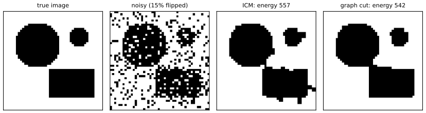
fig_9_S3. Download: PDF · SVG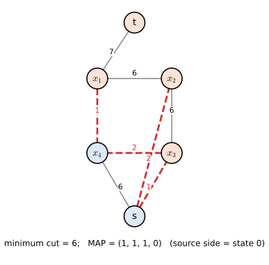
fig_S9_13. Reproduces Murphy (2023), Supplementary Figure 9.13. Download: PDF · SVGThe supplement's Figure S9.14 (\(\alpha\)-expansion and \(\alpha\)-\(\beta\) swap moves) is a schematic, not computed, and is skipped.
Practice problems
Chapter 9 of the book has no end-of-chapter exercises. Here are three short problems with worked solutions.
Problem 9.1. A two-state HMM has \(A=\begin{pmatrix}0.9&0.1\\0.2&0.8\end{pmatrix}\), \(\pi=(0.5,0.5)\), and two observations with local evidence \(\lambda_1=(0.8,0.3)\), \(\lambda_2=(0.1,0.6)\). Compute \(\alpha_1,\alpha_2\), \(p(y_{1:2})\), \(\beta_1\), \(\gamma_1\) and the Viterbi path by hand.
Solution
\(\alpha_{1|0}=\pi\), \(\lambda_1\odot\pi=(0.4,0.15)\), \(Z_1=0.55\), \(\alpha_1=(0.7273,0.2727)\). Predict: \[ \alpha_{2|1}=A^\T\alpha_1=(0.9\cdot0.7273+0.2\cdot0.2727,\ 0.1\cdot0.7273+0.8\cdot0.2727)=(0.7091,0.2909) \]; \(\lambda_2\odot\alpha_{2|1}=(0.07091,0.17455)\), \(Z_2=0.24545\), \(\alpha_2=(0.2889,0.7111)\). So \(p(y_{1:2})=Z_1Z_2=0.55\cdot0.24545=0.135\). Backwards: \(\beta_2=(1,1)\), \[ \beta_1=A(\lambda_2\odot\beta_2)=A(0.1,0.6)^\T=(0.9\cdot0.1+0.1\cdot0.6,\ 0.2\cdot0.1+0.8\cdot0.6)=(0.15,0.50) \]; \(\alpha_1\odot\beta_1=(0.1091,0.1364)\) so \(\gamma_1=(0.4444,0.5556)\), \(\gamma_2=\alpha_2\). Viterbi: \(\delta_1=(0.4,0.15)\); \[ \delta_2(1)=0.1\max(0.4\cdot0.9,\,0.15\cdot0.2)=0.036 \], ancestor 1; \[ \delta_2(2)=0.6\max(0.4\cdot0.1,\,0.15\cdot0.8)=0.6\cdot0.12=0.072 \], ancestor 2. The best end state is 2, so the MAP path is \((2,2)\) with joint probability 0.072; \(\arg\max\gamma\) gives the same path here. A check of the total: \(p(y)\) is the sum of the four path weights, \[ 0.4\cdot0.9\cdot0.1+0.4\cdot0.1\cdot0.6+0.15\cdot0.2\cdot0.1+0.15\cdot0.8\cdot0.6=0.036+0.024+0.003+0.072=0.135. \] The code reproduces all these numbers.
Problem 9.2. A Gaussian MRF on a 3-cycle has \(J=\begin{pmatrix}3&-1&-1\\-1&3&-1\\-1&-1&3\end{pmatrix}\) and \(h=(1,0,0)^\T\). Run Gaussian BP by symmetry: find the fixed-point message precision \(P\), the BP variance of each node, and compare with the exact variance and mean.
Solution
By symmetry all precision messages are equal, \(P=-J_{ij}^2/(J_{ii}+P)=-1/(3+P)\) (each node receives one other message when sending along an edge of a 3-cycle), so \(P^2+3P+1=0\) and \(P=(-3+\sqrt5)/2=-0.382\) (the root with \(|P|\) small, the one reached from \(P=0\)). Each belief combines two incoming messages: precision \(3+2P=3-0.764=2.236\), variance \(1/2.236=0.4472\). The exact covariance is \(J^{-1}=\frac14(I+\mathbf 1\mathbf 1^\T)\) (because \(J=4I-\mathbf 1\mathbf 1^\T\) and \[ (4I-\mathbf 1\mathbf 1^\T)^{-1}=\tfrac14(I+\tfrac{\mathbf 1\mathbf 1^\T}{4-3}) \]), with diagonal \(\tfrac12\). So BP's variance is too small (over-confident): 0.4472 against 0.5. The means from BP converge to \(J^{-1}h=(0.5,0.25,0.25)\), exactly, by Result 9.14. The code runs the iteration and gets 0.44721 and the exact mean.
Problem 9.3. Eliminate the variables of a 5-cycle \(1-2-3-4-5-1\) with \(K\) states each in the order \(1,2,3,4,5\). List the fill-in edges, the maximal cliques, the induced width and the cost (9.92), and draw the junction tree.
Solution
Eliminating 1 joins its neighbours 2 and 5: fill-in edge \(2-5\), clique \(\{1,2,5\}\). Eliminating 2 (now adjacent to 3 and 5) joins \(3-5\): clique \(\{2,3,5\}\). Eliminating 3 (adjacent to 4, 5, already joined): clique \(\{3,4,5\}\). Eliminating 4 and 5 gives the contained cliques \(\{4,5\}\) and \(\{5\}\). So the fill-in edges are \(2-5\) and \(3-5\), the maximal cliques are the three triangles \(\{1,2,5\},\{2,3,5\},\{3,4,5\}\), the width is 2 and the cost \(3K^3\). The junction graph has edge weights \(|\{2,5\}|=2\) between the first two and \(|\{3,5\}|=2\) between the last two, and 1 between the first and third; the maximum-weight spanning tree is the path \(125-235-345\) with separators \(\{2,5\}\) and \(\{3,5\}\) (weight 4). A cycle has treewidth 2, so this is optimal; the code confirms exact treewidth 2 and the three cliques, with cost 24 for \(K=2\).
Demonstrations for this chapter
Each demonstration runs in the browser, with seeded random numbers, and links back to these notes. The ▶ Demo boxes above open them already set to the case under discussion.
| Demonstration | What you can see | Sections and results |
|---|---|---|
| Forwards-backwards and Viterbi in the dishonest casino | Filtered, smoothed and Viterbi curves for the Figure 9.3 rolls or new seeded rolls, while you change the believed transition and loading probabilities; posterior path samples; the Figure 9.6 trellis. Presets: 1 default; 2 sticky loaded die; 3 barely loaded; 4 short window; 5 Viterbi example. | 9.2.2, 9.2.3, 9.2.6, 9.2.7, Result 9.10 |
| Loopy belief propagation on an Ising grid | Beliefs against exact marginals on grids of 5 to 11 squares; synchronous or asynchronous sweeps, damping, coupling strength, spanning tree; convergence and the belief of a chosen spin. Presets: 1 weak coupling; 2 strong, synchronous; 3 damped; 4 asynchronous damped; 5 tree. | 9.4.1, 9.4.4, Results 9.12, 9.13 |
| Variable elimination: choosing the order | Click an elimination order for the 8-variable student network: fill-in edges, clique sizes, width, cost, junction-tree edges, exact marginal by elimination and by enumeration, and a search over all 40,320 orders. Presets: 1 Table 9.1; 2 Table 9.2; 3 min-fill; 4 worst order; 5 all orders. | 9.5.1–9.5.3, 9.6, Results 9.17, 9.19 |
The Python code that produces every figure of this page is code/ch09_message_passing.py (see the code index).
Errors and slips found in the book
Each item was confirmed by recomputation, or is flagged as a possible slip. Items marked (minor) are notational.
- Section 9.2.6.2 (p. 410): "If there is a unique MAP estimate, the above procedure will give the same result as picking \(\hat z_t=\mathrm{arg\,max}_j\gamma_t(j)\), computed by forwards-backwards." This confuses the posterior marginals \(\gamma\) with the max-marginals. The per-time maximiser of \(\gamma\) (MPM) and the MAP path generally differ even when the MAP is unique, as Figure 9.3 itself shows (49 against 60 errors), and as in our casino sample (51 against 57) and in 35 of 40 random sequences of length 60 (Result 9.9). The correct statement (Section 9.3.3.1) is about max-marginals.
- (9.100): \(\mu=K(G^\T\Sigma_p^{-1}\mu_p+H^\T\Sigma_n^{-1}(y-c))\) is missing the inverse: the posterior mean is \(\mu=K^{-1}(\cdots)\), which is what (9.102)–(9.104) use (checked: \(K^{-1}(\cdots)\) equals the mean of 200,000 perturb-and-MAP draws, \(K(\cdots)\) does not).
- (9.73): the interpolation weight \(\gamma_i=(x_i-g_i)/(g_i-g_{i-1})\) should be \((x_i-g_{i-1})/(g_i-g_{i-1})\) for the prediction (9.72) \((1-\gamma_i)z_{i-1}+\gamma_iz_i\) to be an interpolation; (9.71) and (9.74) are energies, not potentials (minor; Filling the gap 9.3).
- (9.60): for a non-root node \(s\) the product should include the message from \(s\)'s parent as well as the other children; as printed (children other than \(t\) only) it is correct only for the root (Section 9.3.2; the following (9.61) is right).
- Figure 9.12 caption: "Nodes 2 and 3 occur more often in the tree because they have higher degree than nodes 1 and 2" should say "than nodes 1 and 4": the degrees of the graph are 2, 3, 3, 2 for nodes 1, 2, 3, 4 (checked by building the computation tree, Result 9.12).
- (9.81): the parity factor is printed as \(\mathbb I(x_s\otimes x_t\otimes x_u=1)\), but codewords have an even number of ones (Section 9.3.3.2 says so), so the constraint should be \(x_s\oplus x_t\oplus x_u=0\), unless \(\otimes\) denotes XNOR (minor).
- Section 9.2.6.3, Figure 9.6: the last \(\delta\) is printed as 0.0022; the exact value is \(0.002205\) (minor, rounding). Section 9.2.3.4: "state conditional log likelihoods \(\lambda_t(j)\)" should be \(\ell_t(j)\) (minor).
- Listing 9.1: inside a function differentiated with JAX the logarithm should be
jnp.log, notnp.log(we did not run JAX; possible slip). Supplement (S9.41)–(S9.47): indices and clique names are inconsistent ("\(\alpha_{t-1})(X_t)\)", clique \(i\) used for the middle clique); (S9.59): the printed matrix has \(-1\) in every row (minor; Filling the gap 9.8); (S9.68) uses \(E_{uv}\) and \(\lambda_{uv}\) but the text then writes \(\lambda_{st}\) (minor).
References
- Murphy, K. P. (2023). Probabilistic Machine Learning: Advanced Topics. MIT Press. Chapter 9 (pp. 401–438) and Supplementary Chapter 9 (pp. 99–122). probml.github.io/pml-book/book2.html.
- Aji, S. M. and McEliece, R. J. (2000). The generalized distributive law. IEEE Transactions on Information Theory, 46(2), 325–343.
- Arnborg, S., Corneil, D. G. and Proskurowski, A. (1987). Complexity of finding embeddings in a \(k\)-tree. SIAM Journal on Algebraic and Discrete Methods, 8, 277–284.
- Bodlaender, H. L. (1993). A tourist guide through treewidth. Acta Cybernetica, 11, 1–21.
- Boykov, Y., Veksler, O. and Zabih, R. (2001). Fast approximate energy minimization via graph cuts. IEEE Transactions on Pattern Analysis and Machine Intelligence, 23(11), 1222–1239.
- Dagum, P. and Luby, M. (1993). Approximating probabilistic inference in Bayesian belief networks is NP-hard. Artificial Intelligence, 60, 141–153.
- Elidan, G., McGraw, I. and Koller, D. (2006). Residual belief propagation: informed scheduling for asynchronous message passing. UAI.
- Frey, B. J. and Dueck, D. (2007). Clustering by passing messages between data points. Science, 315, 972–976.
- Greig, D. M., Porteous, B. T. and Seheult, A. H. (1989). Exact maximum a posteriori estimation for binary images. Journal of the Royal Statistical Society B, 51, 271–279.
- Hazan, T. and Jaakkola, T. (2012). On the partition function and random maximum a-posteriori perturbations. ICML.
- Jensen, F. V. and Jensen, F. (1994). Optimal junction trees. UAI.
- Kschischang, F. R., Frey, B. J. and Loeliger, H.-A. (2001). Factor graphs and the sum-product algorithm. IEEE Transactions on Information Theory, 47(2), 498–519.
- Lauritzen, S. L. and Spiegelhalter, D. J. (1988). Local computations with probabilities on graphical structures and their application to expert systems. Journal of the Royal Statistical Society B, 50, 157–224.
- McEliece, R. J., MacKay, D. J. C. and Cheng, J.-F. (1998). Turbo decoding as an instance of Pearl's belief propagation algorithm. IEEE Journal on Selected Areas in Communications, 16(2), 140–152.
- Mooij, J. M. and Kappen, H. J. (2007). Sufficient conditions for convergence of the sum-product algorithm. IEEE Transactions on Information Theory, 53(12), 4422–4437.
- Murphy, K. P., Weiss, Y. and Jordan, M. I. (1999). Loopy belief propagation for approximate inference: an empirical study. UAI.
- Papandreou, G. and Yuille, A. L. (2011). Perturb-and-MAP random fields: using discrete optimization to learn and sample from energy models. ICCV.
- Pearl, J. (1988). Probabilistic Reasoning in Intelligent Systems. Morgan Kaufmann.
- Rabiner, L. R. (1989). A tutorial on hidden Markov models and selected applications in speech recognition. Proceedings of the IEEE, 77(2), 257–286.
- Shafer, G. R. and Shenoy, P. P. (1990). Probability propagation. Annals of Mathematics and Artificial Intelligence, 2, 327–351.
- Viterbi, A. J. (1967). Error bounds for convolutional codes and an asymptotically optimum decoding algorithm. IEEE Transactions on Information Theory, 13(2), 260–269.
- Wainwright, M. J. and Jordan, M. I. (2008). Graphical models, exponential families, and variational inference. Foundations and Trends in Machine Learning, 1(1–2), 1–305.
- Weiss, Y. (2000). Correctness of local probability propagation in graphical models with loops. Neural Computation, 12, 1–41.
- Weiss, Y. and Freeman, W. T. (2001). Correctness of belief propagation in Gaussian graphical models of arbitrary topology. Neural Computation, 13, 2173–2200.
- Yanover, C. and Weiss, Y. (2004). Finding the \(M\) most probable configurations using loopy belief propagation. NIPS.
- Yedidia, J. S., Freeman, W. T. and Weiss, Y. (2000). Generalized belief propagation. NIPS.
The numerical statements in the text (the casino numbers, the Viterbi example, the code example, the elimination tables and cliques, the treewidth counts, the junction tree calibration, the 3-SAT reduction, the graph-cut example, the LP relaxation and the weak-coupling contraction bound) were confirmed by recomputation and by comparison with brute-force enumeration.