Decision making under uncertainty
Inference ends in a decision. This chapter turns posterior beliefs into actions: the Bayes rule for one-shot problems (and why it is also the best frequentist rule), influence diagrams and the value of information, the Bayesian design of an A/B test, bandits that learn while they earn (upper confidence bounds, Thompson sampling and the logarithmic regret they achieve), Markov decision processes and their planning algorithms (value iteration, policy iteration, linear programming), and active learning, where the decision is which label to buy. The notes prove each result the book states without proof, correct the numerical slips I found (the maximum expected utility of the oil wildcatter, the error rate of the A/B test), and reproduce the computed figures with my own code.
Ch. 1 Introduction Ch. 2 Probability Ch. 3 Statistics Ch. 4 Graphical models Ch. 5 Information theory Ch. 6 Optimisation Ch. 7 Inference algorithms Ch. 8 Gaussian filtering Ch. 9 Message passing Ch. 10 Variational inference Ch. 11 Monte Carlo Ch. 12 MCMC Ch. 13 Sequential Monte Carlo Ch. 14 Predictive models Ch. 15 GLMs Ch. 16 Deep networks Ch. 17 Bayesian neural networks Ch. 18 Gaussian processes Ch. 19 Beyond iid Ch. 20 Generative models Ch. 21 VAEs Ch. 22 Autoregressive models Ch. 23 Normalizing flows Ch. 24 Energy-based models Ch. 25 Diffusion models Ch. 26 GANs Ch. 27 Discovery methods Ch. 28 Latent factor models Ch. 29 State-space models Ch. 30 Graph learning Ch. 31 Nonparametric Bayes Ch. 32 Representation learning Ch. 33 Interpretability Ch. 34 Decision making Ch. 35 Reinforcement learning Ch. 36 Causality
How to read these notes
They follow the book. Sections carry the book's numbers. I keep the book's equation numbers where I restate an equation, e.g. (34.22), (34.43), (34.87). The chapter states many results without proof, so most of the work here is in the gap boxes.
Filling the gaps. Wherever the book states a result without proof (the equivalence of Bayesian and frequentist optimality, the max-marginal estimator, the optimal test size and the regret and error rate of an A/B test, the regret of bandit algorithms and the lower bound, the contraction property and the policy improvement theorem, the two linear programs, the BALD and BatchBALD identities), an orange Filling the gap box gives the full argument. Proofs start hidden. Results already proved in the introductory volume are linked, not repeated.
Figures. Figures 34.2, 34.5, 34.6, 34.8, 34.9, 34.10, 34.13 and 34.15 to 34.18 are reproduced with my own code, and Figure 34.20 in a scaled-down form (the 8 by 8 scikit-learn digits and a small dropout network replace MNIST and a convolutional network). Figures 34.1, 34.3, 34.4, 34.7, 34.11, 34.12, 34.14 and 34.19 are diagrams or recorded data with nothing to compute. Figures 34.21 to 34.23 are my own (regret curves against the Lai-Robbins bound, value iteration as a contraction, and the Bayes-optimal bandit policy by dynamic programming).
The supplement. The supplement chapter S34 ("Multi-step decision problems") contains only a title page in this draft (pages 307 and 308), so there is nothing to cover; Supplement S34 says so.
Main reference
K. P. Murphy, Probabilistic Machine Learning: Advanced Topics, MIT Press (2023; December 2025 draft), Chapter 34, pages 1105–1144 (book page: probml.github.io/pml-book/book2.html). The explanations, derivations, figures and code are my own.
Companion courses
- Probabilistic Machine Learning: An Introduction: Chapter 5 (decision theory) proves that the Bayes rule minimises the posterior risk (Result 5.1), the MAP rule for 0-1 loss (5.1b), Chow's reject rule (5.3), the mean and the median for squared and absolute loss (5.5), that a Bayes rule with constant risk is minimax (5.8) and admissibility (gap 5.19). Section 22.4 proves the regret decomposition and the UCB1 bound (gap 22.13) and has a bandit demo. Section 19.4 covers active learning (gap 19.15 value of information, 19.16 BALD for linear-Gaussian models, 19.17 submodularity and the greedy bound) with an active-learning demo.
- This course: 6.6 Bayesian optimisation (the acquisition functions of the book's Table 34.1), 9.5 variable elimination (the algorithm behind influence-diagram solving), 3.4 conjugate priors, gap 15.4 (the normal-inverse-gamma posterior used by the linear-Gaussian bandit), 5.3.5 total correlation, 17.3.9 deep ensembles (committees) and 19.3 selective prediction. Chapter 35 (reinforcement learning) continues from the Markov decision processes here.
What this chapter adds: the closed forms of the A/B-test quantities with the corrected error rate, the complete Lai-Robbins lower-bound argument, a proof that value iteration, policy iteration and the two linear programs all return the same optimum (checked on a stochastic grid world), the exact Bayes-optimal bandit policy computed by dynamic programming on the belief state, and the BatchBALD total-correlation identity.
The chapter at a glance
- 34.1 The Bayes rule minimises the posterior risk and the Bayes risk (gap 34.1); admissible rules are Bayes rules (gap 34.2); mean, mode, median and quantile (gap 34.3); max-marginals for Hamming loss (gap 34.4); minimum Bayes risk decoding (gap 34.5); fairness criteria clash (gap 34.6).
- 34.2 The oil wildcatter, with corrected numbers (gap 34.7); the value of information (gap 34.8); solving influence diagrams backwards (gap 34.9).
- 34.3 A/B testing: posterior and optimal rule (gap 34.10), expected reward (34.11), optimal test size (34.12), regret (34.13), error rate (34.14).
- 34.4 Bandits: belief states and the Bayes-optimal policy (gap 34.15), the linear-Gaussian posterior (34.16), UCB (34.17), Thompson sampling (34.18), the Lai-Robbins bound (34.19).
- 34.5–34.6 MDPs: returns and value functions (gap 34.20), Bellman equations and the contraction (34.21), the grid world (34.22), POMDP beliefs (34.23), value iteration (34.24), policy iteration (34.25), linear programming (34.26).
- 34.7 Active learning: uncertainty scores (gap 34.27), BALD (34.28), BatchBALD (34.29).
Notation. \(h\) the state of nature, \(a\) an action, \(\ell(h,a)\) a loss, \(\delta\) a decision rule, \(R(\delta)\) a risk, \(\rho\) a posterior risk, \(U=-\ell\) a utility. For bandits \(\mu_a\) is the mean reward of arm \(a\), \(\Delta_a=\mu^*-\mu_a\), \(N_a(T)\) the number of pulls. For MDPs \(\gamma\) is the discount, \(V_\pi,Q_\pi\) value functions, \(T_\pi\) the state transition matrix under \(\pi\).
34.1 Statistical decision theory
p. 1105 Bayesian inference ends with a posterior \(p(h\given x)\) over a hidden quantity \(h\); to act we need a rule that turns it into an action. The standard framework has an agent, a set of actions \(\mathcal A\), data \(x\), a state of nature \(h\in\mathcal H\) and a loss \(\ell(h,a)\). A policy (decision procedure, estimator when \(h\) is a parameter) is a map \(a=\delta(x)\), and its risk is its expected loss. The book cites DeGroot (1970), Berger (1985) and Kochenderfer et al. (2022) for more. The introductory volume treats the same ground at a lower level: pml Chapter 5.
34.1.1 Basics
p. 1105 The optimal policy minimises the risk, \[ \delta^*(\cdot)=\argmin_\delta R(\delta),\qquad R(\delta)=\E\big[\ell(h,\delta(X))\big], \tag{34.1, 34.2} \] but the expectation needs a choice of what is random, the data (frequentist) or the state of nature (Bayesian). The footnote makes a useful point for machine learning: what we can measure is prediction error on future observables, \(\ell(y,\hat f(c))\), not error in the parameters.
34.1.2 Frequentist decision theory
p. 1106 Treat \(h\) as fixed and the data as random. The frequentist risk, and the Bayes (integrated) risk and maximum risk obtained by averaging or maximising it over \(h\), are \[ r(\delta\given h)=\E_{p(x\given h)}\big[\ell(h,\delta(x))\big],\quad R_\pi(\delta)=\E_{\pi(h)}\big[r(\delta\given h)\big],\quad R_{\max}(\delta)=\max_h r(\delta\given h), \tag{34.3, 34.4, 34.5} \] and a minimiser of \(R_{\max}\) is a minimax estimator (34.6). The book notes that minimax estimators are pessimistic (they assume nature is an adversary) and that they equal Bayes estimators under a least favourable prior. Gap 34.1 proves the identities behind these remarks and works out the one case in which everything is explicit, a binomial proportion. The risk functions of several estimators are drawn in the frequentist-risk demo of the introductory volume.
Filling the gap 34.1: Bayes risk two ways, the Bayes rule, the least favourable prior and a binomial minimax estimator pp. 1106–1107, (34.4)–(34.12)
Derivation
Assumptions. The loss is bounded below, \(\ell\ge-c\), so that all expectations exist (possibly \(+\infty\)); \(\mathcal A\) is finite or the minimum over \(a\) is attained measurably. Let \(p(h,x)=\pi(h)p(x\given h)\) and \(p(x)=\int p(h,x)\d h\).
Bayes risk is the average posterior risk (34.11, 34.12). By Tonelli's theorem (Fubini for functions bounded below) the double integral can be done in either order: \[ R_\pi(\delta)=\iint\pi(h)p(x\given h)\,\ell(h,\delta(x))\d x\d h=\int p(x)\Big[\int p(h\given x)\,\ell(h,\delta(x))\d h\Big]\d x=\E_{p(x)}\big[\rho(\delta(x)\given x)\big], \] where \(\rho(a\given x)=\E_{p(h\given x)}\ell(h,a)\) is the posterior risk (34.7). This is the law of iterated expectation, drawn as Figure 34.1 in the book.
The Bayes rule minimises the Bayes risk (34.9). For every \(x\), \(\rho(\delta(x)\given x)\ge\min_a\rho(a\given x)\). Averaging over \(p(x)\) gives \(R_\pi(\delta)\ge\E_{p(x)}\min_a\rho(a\given x)\), with equality for \(\delta^*(x)\in\argmin_a\rho(a\given x)\). So choosing the best action separately for each observed \(x\) (the Bayesian recipe) is also the best policy on average over datasets (the frequentist criterion with a prior), and \[ R_\pi(\delta^*)=\E_{p(x)}\Big[\min_a\rho(a\given x)\Big]. \] Another consequence is the quantity used in the value of information (gap 34.8). See also pml Result 5.1.
Maximum risk and the least favourable prior. Because \(R_\pi(\delta)\) is an average of \(r(\delta\given h)\), \(R_\pi(\delta)\le R_{\max}(\delta)\), and putting \(\pi\) on a point mass at the maximising \(h\) attains it: \(\sup_\pi R_\pi(\delta)=R_{\max}(\delta)\), the identity quoted in the book. Hence for any \(\delta'\) and any prior \(\pi\), \(R_{\max}(\delta')\ge R_\pi(\delta')\ge R_\pi(\delta_\pi)\), where \(\delta_\pi\) is the Bayes rule. If one can find a prior with \(R_\pi(\delta_\pi)=R_{\max}(\delta_\pi)\) (a least favourable prior; this happens when \(r(\delta_\pi\given h)\) is constant, an equaliser rule, or at least equals its maximum on the support of \(\pi\)), then \(R_{\max}(\delta')\ge R_{\max}(\delta_\pi)\) for every \(\delta'\), so \(\delta_\pi\) is minimax (pml Result 5.8).
Binomial proportion. Let \(X\sim\mathrm{Bin}(n,p)\), squared loss, prior \(\Beta(a,b)\). The posterior is \(\Beta(a+x,b+n-x)\) and the Bayes rule is the posterior mean \(\hat p=(x+a)/(n+a+b)\). Its frequentist risk is variance plus squared bias, with \(c=n+a+b\): \[ r(\hat p\given p)=\frac{np(1-p)+\big(a-(a+b)p\big)^2}{c^2}=\frac{\big((a+b)^2-n\big)p^2+\big(n-2a(a+b)\big)p+a^2}{c^2}. \] The risk is constant in \(p\) iff both coefficients vanish: \((a+b)^2=n\) and \(2a(a+b)=n\), i.e. \(a=b=\sqrt n/2\). Then \(r\equiv a^2/c^2=\dfrac{n}{4(n+\sqrt n)^2}\), the estimator \((x+\sqrt n/2)/(n+\sqrt n)\) is Bayes with constant risk, hence minimax by the argument above, and \(\Beta(\sqrt n/2,\sqrt n/2)\) is the least favourable prior. For \(n=25\) the minimax risk is \(0.00694\), against a worst-case risk \(1/(4n)=0.0100\) for the maximum likelihood estimator \(x/n\) (reached at \(p=\tfrac12\)); the minimax rule is better near \(p=\tfrac12\) and worse near 0 and 1, the usual price of equalising the risk. A grid search over \(\Beta(a,b)\) posterior-mean estimators confirms that none has a smaller maximum risk.
Not every minimax estimator is Bayes for a proper prior: the Gaussian sample mean is minimax only as a limit of Bayes rules (pml Result 5.8(d)).
34.1.3 Bayesian decision theory
pp. 1106–1107 The Bayesian treats the data as fixed and \(h\) as random. The posterior risk of an action and of an estimator are \[ \rho_\pi(a\given x)=\E_{p_\pi(h\given x)}\big[\ell(h,a)\big],\qquad \delta^*(x)=\argmin_{a\in\mathcal A}\rho_\pi(a\given x), \tag{34.7, 34.9} \] so only the optimal action for the observed \(x\) is needed. With a utility \(U=-\ell\) this is the maximum expected utility principle \(\delta^*(x)=\argmax_a\E_h[U(h,a)]\) (34.10), the form used in Section 34.2.
34.1.4 Frequentist optimality of the Bayesian approach
p. 1107 Equations (34.11) and (34.12) say that the posterior-risk rule also minimises the Bayes risk; this is proved in gap 34.1. The book adds that every admissible policy is a Bayes policy for some, possibly improper, prior (Wald 1947). Gap 34.2 proves this for a finite parameter space and shows the converse direction (a Bayes rule for a prior that charges every state is admissible). The practical lesson is the one the book draws: the Bayesian approach is constructive (it tells you how to build the estimator), while the frequentist approach lets you use any estimator and only analyses it.
Filling the gap 34.2: admissible rules are Bayes rules (finite parameter space), and Bayes rules are admissible p. 1107, Wald (1947)
Derivation
Setting. \(\mathcal H=\{h_1,\dots,h_k\}\), finite data and action sets, rules allowed to randomise. The risk point of a rule is \(r(\delta)=(r(\delta\given h_1),\dots,r(\delta\given h_k))\in\R^k\). The set \(S\) of risk points is convex (a mixture of two rules has the mixture of their risk points) and \(\delta_1\) dominates \(\delta_2\) when \(r(\delta_1)\le r(\delta_2)\) coordinatewise with at least one strict inequality.
Bayes rule for a strictly positive prior is admissible. Suppose \(\delta\) is Bayes for \(\pi\) with \(\pi_i>0\) for all \(i\), and \(\delta'\) dominates it. Then \(R_\pi(\delta')=\sum_i\pi_ir_i(\delta')<\sum_i\pi_ir_i(\delta)=R_\pi(\delta)\), because every weight is positive and one inequality is strict. This contradicts the minimality of \(R_\pi(\delta)\). So no rule dominates \(\delta\).
Admissible implies Bayes for some prior. Let \(\delta\) be admissible, \(r^*=r(\delta)\), and \(A=\{y\in\R^k:y_i<r^*_i\ \forall i\}\), an open convex set. If a point of \(S\) lay in \(A\) it would strictly dominate \(\delta\), so \(S\cap A=\emptyset\). By the separating hyperplane theorem there are \(\lambda\ne0\) and \(c\) with \(\lambda^\T y\le c\le\lambda^\T s\) for all \(y\in A\), \(s\in S\). If some \(\lambda_i<0\), letting \(y_i\to-\infty\) inside \(A\) sends \(\lambda^\T y\to+\infty\), contradicting \(\lambda^\T y\le c\); so \(\lambda\ge0\), and we may normalise \(\sum\lambda_i=1\). Since \(r^*\) is in the closure of \(A\), \(\lambda^\T r^*\le c\le\lambda^\T r(\delta')\) for every rule \(\delta'\). Thus \(\delta\) minimises \(R_\lambda\), i.e. it is a Bayes rule for the prior \(\lambda\). The prior may give zero weight to some states: those rules are Bayes only for a prior with a smaller support, the finite analogue of "improper" in the book's statement. For infinite \(\mathcal H\) the same idea requires a limiting argument (Wald 1947; Ferguson 1967; the book also cites a more general version, its reference [DR21]).
Example. Two states, three observations with likelihoods \((0.6,0.3,0.1)\) and \((0.1,0.3,0.6)\), 0-1 loss: of the eight deterministic rules, four are admissible, and each of them is the Bayes rule for some prior weight on a grid of 2001 values; the other four are dominated.
34.1.5 Examples of one-shot decision making problems
34.1.5.1 Classification
p. 1108 With states and actions both the class labels and the 0-1 loss \(\ell_{01}(y^*,\hat y)=\ind(y^*\ne\hat y)\) (34.13, 34.14), the posterior risk is \(1-p(\hat y\given x)\) (34.15), so the optimal action is the most probable label, the MAP estimate (34.16). Unequal costs and a reject option lead to thresholds and to selective prediction (Section 19.3.3 of the book, notes); both are derived in pml Result 5.3.
34.1.5.2 Regression
p. 1108 With a scalar state and action and the squared loss \(\ell_2(h,y)=(h-y)^2\) (34.17), \(\rho(y\given x)=\E[h^2\given x]-2y\E[h\given x]+y^2\) (34.18), whose derivative vanishes at the posterior mean (34.19), the minimum mean squared error (MMSE) estimate.
34.1.5.3 Parameter estimation
p. 1109 For a parameter vector, squared loss again gives the posterior mean and 0-1 loss the posterior mode, \(\hat\theta=\argmax_\theta p(\theta\given\mathcal D)\) (34.20).
Filling the gap 34.3: mean, mode, median and quantile as Bayes actions pp. 1108–1109, (34.15)–(34.20)
Derivation
The mode (0-1 loss), the mean (squared loss) and the median (absolute loss) are proved in pml Results 5.1b and 5.5. Two short additions.
The posterior mean is a minimum, with value equal to the posterior variance. Expand \(\E[(h-y)^2\given x]=\var[h\given x]+(\E[h\given x]-y)^2\) (add and subtract the mean; the cross term has mean zero). This is a parabola in \(y\) with minimum at \(y=\E[h\given x]\) (so the stationary point in (34.19) is a minimum) and minimum value \(\var[h\given x]\). For a vector parameter the squared error is a sum over components, so the optimum is the vector of marginal posterior means.
Asymmetric linear loss gives a quantile. Let \(\ell(h,a)=c_u(h-a)^+ +c_o(a-h)^+\) (cost \(c_u\) per unit of under-prediction, \(c_o\) per unit of over-prediction; the newsvendor problem). With \(F\) the posterior cdf, \(\rho'(a)=-c_u\Pr(h>a)+c_o\Pr(h<a)=-c_u+(c_u+c_o)F(a)\), which is nondecreasing, so the minimiser solves \(F(a)=c_u/(c_u+c_o)\): the posterior quantile at level \(c_u/(c_u+c_o)\). With \(c_u=c_o\) this is the median. The mean, median and mode coincide for a symmetric unimodal posterior and differ otherwise, so the choice of loss, not of estimator, is the real modelling decision.
34.1.5.4 Estimating discrete parameters
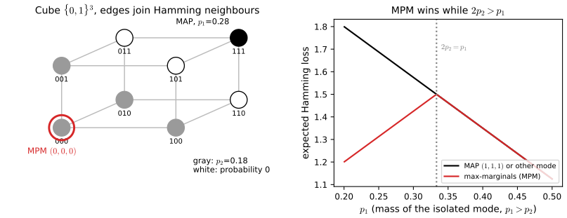
pp. 1109–1110 The 0-1 loss gives no partial credit for a parameter vector with some correct components. The Hamming loss \(\ell(\theta,\hat\theta)=\sum_d\ind(\theta_d\ne\hat\theta_d)\) (34.21) does, and its optimal estimator is the vector of maximisers of the marginals, the MPM estimate, \[ \hat\theta_d=\argmax_{\theta_d}\int p(\theta\given\mathcal D)\d\theta_{-d}. \tag{34.22} \] Figure 34.2 shows a distribution on \(\{0,1\}^3\) whose mode \((1,1,1)\) is isolated, while four mutually connected states carry most of the mass; there \(p(\theta_j=0)=3p_2\) and \(p(\theta_j=1)=p_1+p_2\), and the MPM is \((0,0,0)\) when \(2p_2>p_1\). Proofs, and the claim that the MPM is a "centroid" estimator, are in gap 34.4.
Filling the gap 34.4: Hamming loss gives the max-marginals; the MPM is the centroid estimator pp. 1109–1110, (34.21), (34.22)
Derivation
(34.22). The posterior risk of \(\hat\theta\) is \(\sum_d\Pr(\theta_d\ne\hat\theta_d\given\mathcal D)=\sum_d\big(1-p(\theta_d=\hat\theta_d\given\mathcal D)\big)\), a sum of terms each depending on one coordinate of \(\hat\theta\) only. It is minimised by minimising each term separately, i.e. by choosing for each \(d\) the value with the largest marginal posterior probability. The computation needs a marginalisation followed by a maximisation, so it uses the whole posterior, not only its mode.
Centroid estimator. For binary \(\theta\in\{0,1\}^D\) the Hamming distance equals the squared Euclidean distance, \(\ind(\theta_d\ne\hat\theta_d)=(\theta_d-\hat\theta_d)^2\). With \(\mu_d=\Pr(\theta_d=1\given\mathcal D)\) the posterior mean, \(\E\|\theta-\hat\theta\|^2=\|\hat\theta-\mu\|^2+\sum_d\mu_d(1-\mu_d)\). The second term does not depend on \(\hat\theta\), so minimising the expected Hamming loss is the same as choosing the vertex of the cube closest to the posterior mean, which is \(\hat\theta_d=\ind(\mu_d>\tfrac12)\): the MPM is the closest valid configuration to the centre of mass, whereas the mean itself has fractional entries.
The cube of Figure 34.2. The state \(L=(1,1,1)\) has mass \(p_1\), the four gray states \(000,100,010,001\) have mass \(p_2\) each, the other three states have mass 0, so \(p_1+4p_2=1\). Then \(p(\theta_j=1)=p_1+p_2\) (the state \(L\) and the one gray state with a 1 in position \(j\)). The expected Hamming loss of the MAP state \(L\) is \(9p_2\): the state \(000\) is at distance 3 from \(L\) and each of the three single-1 states at distance 2, so the loss is \(3p_2+3\cdot2p_2\). That of \((0,0,0)\) is \(3p_1+3p_2\). The MPM is better iff \(3p_1+3p_2<9p_2\), i.e. \(p_1<2p_2\), i.e. \(p_1<\tfrac13\). For \(p_1=0.28\), \(p_2=0.18\): MAP \(1.62\), MPM \(1.38\) (right panel of the figure).
34.1.5.5 Structured prediction
pp. 1110–1111 When the action is a structured object (a word sequence, a set of labels), probable outputs must also be internally consistent, and the loss may encode costs that differ across mistakes. Given a loss, the optimal action is found by minimum Bayes risk (MBR) decoding, \[ \hat y=\argmin_{\hat y\in\mathcal Y}\sum_{y\in\mathcal Y}p(y\given x)\,\ell(y,\hat y), \tag{34.23} \] and, because the sum over \(\mathcal Y\) is intractable, it is approximated from samples \(y_m\sim p(y\given x)\), the empirical MBR of the book's references [Pre+17a] (computer vision) and [Fre+22] (machine translation). Gap 34.5 shows why the sample version works and points out that the weights printed in (34.24) should be uniform.
Filling the gap 34.5: why empirical MBR works, and the weights in (34.24) p. 1110, (34.23), (34.24)
Derivation
(34.23) is the Bayes action. It is (34.9) with the posterior \(p(y\given x)\) and a loss on outputs; the printed "min" over \(\hat y\) should be "argmin".
Monte Carlo version. If \(y_1,\dots,y_M\sim p(y\given x)\) are independent, then for each fixed candidate \(c\), \(\hat\rho(c)=\frac1M\sum_j\ell(y_j,c)\) is an unbiased estimate of the risk \(\rho(c)=\sum_yp(y\given x)\ell(y,c)\), consistent by the law of large numbers. For a finite candidate set (here the samples themselves), a union bound over the candidates, with Hoeffding's inequality for a bounded loss \(\ell\in[0,L]\), gives \(\Pr(\max_c|\hat\rho(c)-\rho(c)|>\epsilon)\le2|\mathcal C|e^{-2M\epsilon^2/L^2}\), so the empirical minimiser has risk within \(2\epsilon\) of the best candidate with high probability, and equals the exact minimiser if the best candidate is unique and \(\epsilon\) is below half the gap.
The weights in (34.24). The printed estimator is \(\sum_jp(y_j\given x)\ell(y_j,y_i)\). For \(y_j\sim p\), its expectation is \(\sum_yp(y\given x)^2\ell(y,y_i)\), which is not the risk: it up-weights an outcome a second time. The right estimator is the unweighted average \(\frac1M\sum_j\ell(y_j,y_i)\); weights proportional to \(p(y_j\given x)\) are appropriate only when the \(y_j\) are a fixed list (an N-best list) rather than draws, and then they must be normalised, \(p(y_j)/\sum_ip(y_i)\). A numerical example: for \(y\in\{0,\dots,4\}\) with probabilities \((0.1,0.3,0.15,0.25,0.2)\) and absolute loss, 4000 samples and the uniform average return the exact median 2; the printed weighted sum differs from the risk by more than 0.05 at some candidates.
34.1.5.6 Fairness
pp. 1111–1112 For a binary classifier with true label \(Y\), prediction \(\hat Y\) and sensitive attribute \(S\), the book lists equal opportunity (equal true positive rates across groups), equalised odds (equal true and false positive rates) and statistical parity (\(p(\hat Y=1\given S)\) independent of \(S\)), and notes that many fairness definitions conflict (Kleinberg 2018). Each is an equality constraint on the group-wise confusion matrices, so imposing it can only raise the minimum expected loss relative to the unconstrained Bayes rule; gap 34.6 shows that two of the criteria cannot hold together except in degenerate cases.
Filling the gap 34.6: the fairness criteria are incompatible when base rates differ p. 1111
Derivation
In group \(s\) let \(p_s=\Pr(Y=1\given S=s)\) (the base rate), \(\mathrm{TPR}_s=\Pr(\hat Y=1\given Y=1,S=s)\), \(\mathrm{FPR}_s=\Pr(\hat Y=1\given Y=0,S=s)\) and \(\mathrm{PPV}_s=\Pr(Y=1\given\hat Y=1,S=s)\).
A bookkeeping identity. By Bayes' rule \(\mathrm{PPV}_s=\dfrac{\mathrm{TPR}_sp_s}{\mathrm{TPR}_sp_s+\mathrm{FPR}_s(1-p_s)}\). Solving for the false positive rate, \[ \mathrm{FPR}_s=\frac{p_s}{1-p_s}\cdot\frac{1-\mathrm{PPV}_s}{\mathrm{PPV}_s}\cdot\mathrm{TPR}_s. \] Equalised odds and equal predictive value cannot both hold. Suppose TPR, FPR and PPV are the same in both groups, with \(\mathrm{TPR}>0\) and \(0<\mathrm{PPV}<1\) (the classifier is neither useless nor perfect). The identity then forces \(p_0/(1-p_0)=p_1/(1-p_1)\), i.e. \(p_0=p_1\). So when base rates differ, a non-trivial classifier must violate equalised odds or predictive parity.
Equalised odds and statistical parity. With common \(\mathrm{TPR}=t\) and \(\mathrm{FPR}=f\), \(\Pr(\hat Y=1\given S=s)=f+(t-f)p_s\). This is the same in both groups iff \((t-f)(p_0-p_1)=0\): either the base rates agree or \(t=f\), a classifier whose prediction is independent of the label.
Each criterion is nonetheless a legitimate constraint to impose on the Bayes decision problem; the point is that they cannot all be imposed at once. The identity was checked on 200 random confusion matrices.
34.2 Decision (influence) diagrams
p. 1112 A multi-stage decision problem can be drawn as an influence diagram: a directed graphical model (Chapter 4) with extra decision nodes (rectangles) and utility nodes (diamonds) beside the chance nodes (ovals). An arc into a decision node is an information arc: the value of that parent is known when the decision is made. Figure 34.4 of the book draws the three diagrams of this section; they are drawings and are not reproduced.
34.2.1 Example: oil wildcatter
pp. 1112–1113 Decide whether to drill (\(d=1\)) or not (\(d=0\)) at a site that is dry (\(o=0\)), wet (\(o=1\)) or soaking (\(o=2\)), with prior \(p(o)=(0.5,0.3,0.2)\) and utility table \[ U(d,o)=\begin{pmatrix}0&0&0\\-70&50&200\end{pmatrix}\ (\text{rows }d=0,1). \] The prior expected utility of each action, \(\EU(d)=\sum_op(o)U(d,o)\) (34.25), is \(0\) for not drilling and \(0.5(-70)+0.3(50)+0.2(200)=20\) for drilling, so \(\MEU=\max_d\EU(d)=20\) and the optimal action is to drill (34.26).
34.2.2 Information arcs
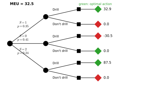
pp. 1113–1114 Now a noisy sounding \(s\in\{0,1,2\}\) (diffuse, open, closed reflection pattern) with likelihood \(p(s\given o)\) below is seen before the decision (Figure 34.4b: an arc \(O\to S\), and an information arc \(S\to D\)). \[ p(s\given o)=\begin{pmatrix}0.6&0.3&0.1\\0.3&0.4&0.3\\0.1&0.4&0.5\end{pmatrix}\ (\text{rows }o). \] The posterior expected utility is \(\EU(d\given s)=\sum_op(o\given s)U(o,d)\) (34.27). The marginal of the sounding is \(p(s)=(0.41,0.35,0.24)\) and the posterior of the oil state given \(s=0\) is \((0.732,0.219,0.049)\). The optimal policy drills exactly when \(s\ge1\), and the maximum expected utility before seeing the sounding is \(\MEU=\sum_sp(s)\max_d\EU(d\given s)\) (34.28). With \(\EU(d{=}1\given s)=(-30.5,\ 32.857,\ 87.5)\) this is \[ \MEU=0.41\cdot0+0.35\cdot32.857+0.24\cdot87.5=\mathbf{32.5}. \tag{34.29, corrected} \] The book prints 32.2 (and so a value of information of 12.2); the correct values are 32.5 and 12.5, as gap 34.7 shows, and as the decision tree of Figure 34.5 displays.
Filling the gap 34.7: the wildcatter, step by step, and a slip in (34.29) pp. 1112–1114, (34.25)–(34.29)
Derivation
Marginal of the sounding. \(p(s)=\sum_op(o)p(s\given o)\): \(s=0\): \(0.5\cdot0.6+0.3\cdot0.3+0.2\cdot0.1=0.41\); \(s=1\): \(0.15+0.12+0.08=0.35\); \(s=2\): \(0.05+0.09+0.10=0.24\).
A shortcut that avoids the posteriors. Since \(p(o\given s)p(s)=p(o)p(s\given o)\), \(p(s)\,\EU(d\given s)=\sum_op(o)p(s\given o)U(d,o)\), the unnormalised joint utility. For drilling these are \(s=0\): \(-70(0.30)+50(0.09)+200(0.02)=-21+4.5+4=-12.5\); \(s=1\): \(-70(0.15)+50(0.12)+200(0.08)=-10.5+6+16=11.5\); \(s=2\): \(-70(0.05)+50(0.09)+200(0.10)=-3.5+4.5+20=21\). Not drilling gives 0 for every \(s\). Hence \[ \MEU=\sum_s\max\{0,\ p(s)\EU(1\given s)\}=0+11.5+21=32.5, \] with the policy "drill iff \(s\ge1\)". Dividing by \(p(s)\) recovers the book's \(\EU(1\given s)=-30.5,32.857,87.5\), and \(0.35\cdot32.857=11.5\), exactly.
The slip. \(0.35\cdot32.9+0.24\cdot87.5=11.52+21=32.5\) even with the book's rounded numbers, so the printed 32.2 in (34.29), and the value of information 12.2 derived from it, cannot be right; the value of the sounding is \(32.5-20=12.5\). Enumerating all eight policies \(d(s)\) confirms 32.5 as the maximum.
34.2.3 Value of information
pp. 1114–1115 If the test is optional (the node \(T\) in Figure 34.4c) it is worth taking when its cost is below the gain in maximum expected utility, \(\mathrm{VPI}=\MEU(G+S\to D)-\MEU(G)\) (34.30). With \(\MEU(G)=20\) this is \(32.5-20=12.5\). The book calls this quantity the value of perfect information; strictly, it is the expected value of sample information (the sounding is a noisy reading), and the value of perfect information, observing \(O\) itself, is larger (gap 34.8).
Filling the gap 34.8: the value of information is non-negative and at most the value of perfect information pp. 1114–1115, (34.30)
Derivation
Let \(S\) be an observation with \(p(o,s)=p(o)p(s\given o)\). Define \(\MEU_0=\max_d\sum_op(o)U(d,o)\), \(\MEU_S=\sum_s\max_d\sum_op(o,s)U(d,o)\) and \(\MEU_O=\sum_op(o)\max_dU(d,o)\) (the value of acting knowing the state). The expected value of sample information is \(\EVSI=\MEU_S-\MEU_0\) and the expected value of perfect information is \(\EVPI=\MEU_O-\MEU_0\).
\(\EVSI\ge0\). For each fixed \(d\), \(\sum_s\sum_op(o,s)U(d,o)=\sum_op(o)U(d,o)\). Since a maximum of a sum is at most the sum of maxima, \(\max_d\sum_s F(d,s)\le\sum_s\max_dF(d,s)\) with \(F(d,s)=\sum_op(o,s)U(d,o)\), i.e. \(\MEU_0\le\MEU_S\). Equality holds iff one action is optimal for every \(s\) (the observation never changes the decision). Compare pml gap 19.15.
\(\EVSI\le\EVPI\). For each \(s\) and \(d\), \(\sum_op(o,s)U(d,o)\le\sum_op(o,s)\max_{d'}U(d',o)\); maximise over \(d\) on the left and sum over \(s\): \(\MEU_S\le\sum_s\sum_op(o,s)\max_{d'}U(d',o)=\MEU_O\).
The wildcatter. Knowing \(o\) would let the wildcatter drill only if \(o\ge1\): \(\MEU_O=0.3\cdot50+0.2\cdot200=55\), so \(\EVPI=55-20=35\), well above \(\EVSI=12.5\). The ordering \(0\le\EVSI\le\EVPI\) holds for every finite problem (checked on 300 random utility tables, priors and sensors). So the test is worth buying if it costs less than 12.5, and no experiment about \(O\) could be worth more than 35.
34.2.4 Computing the optimal policy
p. 1115 In general an optimal policy is found by a modified variable elimination (Lauritzen and Nilsson 2001; Kjaerulff and Madsen 2008): work backwards from the last decision, assuming every later decision is optimal. For a chain (a Markov decision process) this is Bellman's equation (Section 34.5.5). Gap 34.9 explains why the order of eliminating chance and decision nodes matters.
Filling the gap 34.9: why a maximisation does not commute with a sum, and backward induction p. 1115
Derivation
The order of operators encodes who knows what. Without the information arc the wildcatter's value is \(\max_d\sum_s\sum_op(o,s)U(d,o)=20\): the decision is made before \(S\) is seen, so the sum over \(s\) is inside the maximum. With the arc the value is \(\sum_s\max_d\sum_op(o,s)U(d,o)=32.5\): the maximum is chosen separately for each \(s\), inside the sum over \(s\). Since \(\max_d\sum_sF\le\sum_s\max_dF\), observing can only help (gap 34.8), and the two orders genuinely differ, so variable elimination has to respect the temporal order of the diagram: sum out a chance variable only after every decision that precedes it has been maximised over, and take the maximum over a decision with respect to the variables observed before it.
Backward induction. Consider a chain \(s_0,a_0,s_1,a_1,\dots,s_T\) with the decision \(a_t\) allowed to depend on the history up to \(s_t\) and total utility \(\sum_tr(s_t,a_t)\). For any policy, the expected total utility splits as the expected utility of the first \(T-1\) steps plus the expected last reward. The last decision \(a_{T-1}\) affects only the last term, and given the history its best choice is \(\max_{a}\big[r(s_{T-1},a)\big]\), independent of how the earlier decisions were taken. Replace the last term by this maximum, and the same argument applies to \(a_{T-2}\) with the "terminal value" \(V_{T-1}(s)\), and so on: \[ V_T\equiv0,\qquad V_t(s)=\max_a\Big[r(s,a)+\sum_{s'}p(s'\given s,a)V_{t+1}(s')\Big]. \] By induction \(V_0\) is the maximum over all history-dependent policies, and the maximising actions form an optimal Markov policy. This is the finite-horizon Bellman equation, and the discounted infinite-horizon version of Section 34.5.5 is its limit.
34.3 A/B testing
p. 1115 To choose between a control (A, \(j=0\)) and a treatment (B, \(j=1\)) an A/B test applies each to \(n_0\) and \(n_1\) members of a population of size \(N\), measures the rewards, then rolls out the winner to the remaining \(N-n_0-n_1\) members ("test and roll"). Larger tests make the choice more reliable but spend more people on possibly inferior actions: the exploration-exploitation trade-off. The book follows Feit and Berman (2019); two things are to be decided, the rule and the test sizes. The A/B test size demo lets you change every quantity below (preset 2 raises the noise, preset 4 shrinks the population).
34.3.1 A Bayesian approach
p. 1115 The reward of the \(i\)th unit in group \(j\) is \(Y_{ij}\sim\N(\mu_j,\sigma_j^2)\) with known variance, and the prior is \(\mu_j\sim\N(m_j,\tau_j^2)\). Empirical Bayes can set \(m_j,\tau_j\) from past tests (Section 34.3.2).
34.3.1.1 Optimal policy
p. 1116 The optimal rule deploys the arm with the larger posterior mean, \[ \pi^*(y_1,y_0)=\ind\big(\E[\mu_1\given y_1]\ge\E[\mu_0\given y_0]\big), \tag{34.31} \] and the posteriors are Gaussian, \(p(\mu_j\given y_j,n_j)=\N(\mu_j\given\hat m_j,\hat\tau_j^2)\) with \[ \frac1{\hat\tau_j^2}=\frac{n_j}{\sigma_j^2}+\frac1{\tau_j^2},\qquad \frac{\hat m_j}{\hat\tau_j^2}=\frac{n_j\bar y_j}{\sigma_j^2}+\frac{m_j}{\tau_j^2}, \tag{34.32–34.34} \] where \(\bar y_j\) is the sample mean of group \(j\) (the book writes \(y_j\)). In the fully symmetric case this is "pick the winner", \(\pi^*=\ind(\bar y_1>\bar y_0)\) (34.35); when sample sizes or priors differ the shrinkage differs between the arms and the rule is no longer simply the larger sample mean. Gap 34.10 gives the proofs.
Filling the gap 34.10: the Gaussian posterior, the optimal rule and "pick the winner" pp. 1116, (34.31)–(34.35)
Derivation
Posterior (34.32–34.34). The likelihood of \(n\) independent \(\N(\mu,\sigma^2)\) observations is, as a function of \(\mu\), proportional to \(\exp\{-\frac{n}{2\sigma^2}(\bar y-\mu)^2\}\) (expand \(\sum_i(y_i-\mu)^2=\sum_i(y_i-\bar y)^2+n(\bar y-\mu)^2\); the first term does not involve \(\mu\)). Multiplying by the prior \(\exp\{-\frac1{2\tau^2}(\mu-m)^2\}\) and collecting terms in \(\mu\) gives \(\exp\{-\frac12[(\frac n{\sigma^2}+\frac1{\tau^2})\mu^2-2(\frac{n\bar y}{\sigma^2}+\frac m{\tau^2})\mu]+\mathrm{const}\}\), a Gaussian with the stated precision and precision-weighted mean (complete the square). Equivalently \(\hat m=m+w(\bar y-m)\) with shrinkage weight \(w=\dfrac{\tau^2}{\tau^2+\sigma^2/n}\in(0,1)\).
The rule (34.31). After the test, the units of the roll phase are the only ones still to be assigned. Deploying arm \(j\) gives expected reward \((N-n_0-n_1)\E[\mu_j\given\text{data}]\); the test-phase reward is sunk and does not depend on the choice. The Bayes action under (34.10) therefore picks the larger posterior mean (ties arbitrary).
Symmetric case (34.35). If \(n_0=n_1\), \(m_0=m_1\), \(\tau_0=\tau_1\), \(\sigma_0=\sigma_1\), then \(\hat m_j=m+w(\bar y_j-m)\) with the same \(w>0\), so \(\hat m_1>\hat m_0\iff\bar y_1>\bar y_0\). In the unsymmetric case the arm with fewer units has \(w\) smaller, so a given sample mean is pulled further towards its prior mean; the larger sample mean can lose.
34.3.1.2 Optimal sample size
pp. 1116–1117 The prior expected reward of the test phase is \(\E[R_{\mathrm{test}}]=n_0m_0+n_1m_1\) (34.36). The roll phase earns, for the optimal rule, \[ \E[R_{\mathrm{roll}}]=(N-n_1-n_0)\Big(m_1+e\,\Phi\big(\tfrac ev\big)+v\,\varphi\big(\tfrac ev\big)\Big),\quad e=m_0-m_1,\quad v=\sqrt{\frac{\tau_1^4}{\tau_1^2+\sigma_1^2/n_1}+\frac{\tau_0^4}{\tau_0^2+\sigma_0^2/n_0}} \tag{34.39, 34.40} \] (the book writes \(\tilde e,\tilde v\) for the ratios), where \(\varphi,\Phi\) are the standard normal density and cdf. In the symmetric case (\(n_0=n_1=n\), common \(m,\tau,\sigma\)) this becomes \[ \E[R_{\mathrm{roll}}]=(N-2n)\Big(m+\frac{\tau^2}{\sqrt\pi\sqrt{\tau^2+\sigma^2/n}}\Big),\qquad \E[R]=Nm+(N-2n)\frac{\tau^2}{\sqrt\pi\sqrt{\tau^2+\sigma^2/n}}. \tag{34.41, 34.42} \] The first part of (34.41), \((N-2n)m\), is what is expected before learning anything; the second is the gain from picking the better arm, which grows with \(n\) while the number of people who benefit shrinks like \(N-2n\). The maximiser of (34.42) is \[ n^*=\sqrt{\frac N4u^2+\Big(\frac34u^2\Big)^2}-\frac34u^2\ \le\ \frac{\sqrt N\,\sigma}{2\tau},\qquad u^2=\frac{\sigma^2}{\tau^2}. \tag{34.43} \] The test size rises with the noise \(\sigma\) and falls with the expected effect size \(\tau\). Gap 34.11 derives (34.39)–(34.42) and gap 34.12 derives (34.43). In both, the extraction of (34.43) in the book is easy to misread; the formula above is the one that reproduces the book's own number \(n^*=2284\).
Filling the gap 34.11: the expected reward of the roll phase (34.37)–(34.42) pp. 1116–1117
Derivation
Reduction to posterior means. The roll-phase reward under rule \(\pi^*\) is \((N-n_0-n_1)\mu_J\) where \(J\) is the chosen arm. By the tower property, \(\E[\mu_J]=\E\big[\E[\mu_J\given\text{data}]\big]=\E[\max(\hat m_0,\hat m_1)]\), since \(J\) is a function of the data and picks the larger posterior mean.
Distribution of the posterior mean before the test. Marginally (prior predictive) \(\bar y_j\sim\N(m_j,\tau_j^2+\sigma_j^2/n_j)\). Since \(\hat m_j=m_j+w_j(\bar y_j-m_j)\) with \(w_j=\tau_j^2/(\tau_j^2+\sigma_j^2/n_j)\) (gap 34.10), \(\hat m_j\sim\N(m_j,v_j^2)\) with \[ v_j^2=w_j^2\Big(\tau_j^2+\frac{\sigma_j^2}{n_j}\Big)=\frac{\tau_j^4}{\tau_j^2+\sigma_j^2/n_j}. \] (Equivalently, \(v_j^2\) is the prior variance \(\tau_j^2\) minus the expected posterior variance \(\hat\tau_j^2\).) The two arms are independent, so \(W=\hat m_0-\hat m_1\sim\N(e,v^2)\) with \(e=m_0-m_1\) and \(v^2=v_0^2+v_1^2\), the quantity in (34.40).
The maximum of two Gaussians. \(\max(\hat m_0,\hat m_1)=\hat m_1+W^+\) with \(W^+=\max(W,0)\). Write \(W=e+vZ\), \(Z\sim\N(0,1)\). Then \(\E W^+=\int_{-e/v}^\infty(e+vz)\varphi(z)\d z=e\,\Phi(e/v)+v\,\varphi(e/v)\), using \(\int_{-c}^\infty z\varphi(z)\d z=\varphi(c)\). Hence \(\E\max(\hat m_0,\hat m_1)=m_1+e\Phi(e/v)+v\varphi(e/v)\): this is (34.39).
Symmetric case. \(e=0\), \(v^2=2\tau^4/(\tau^2+\sigma^2/n)\), and \(\varphi(0)=1/\sqrt{2\pi}\), so \(v\varphi(0)=\tau^2/(\sqrt\pi\sqrt{\tau^2+\sigma^2/n})\), which is (34.41) (the book's form \(\sqrt2\tau^2/(\sqrt\pi\sqrt{2\tau^2+2\sigma^2/n})\) is the same number). Adding the test-phase reward \(2nm\) gives (34.42). The formula was confirmed by simulating the whole procedure (draw \(\mu_0,\mu_1\) from the prior, the data, the rule, the total reward) for the book's example and for an unsymmetric example with different priors, noise levels and sample sizes: the simulated means agree with (34.39) and (34.42) within Monte Carlo error.
Filling the gap 34.12: the optimal test size (34.43) p. 1117
Derivation
Maximise \(f(n)=(N-2n)g(n)\) over \(0<n<N/2\), where \(g(n)=\dfrac{\tau^2}{\sqrt\pi}\dfrac{\sqrt n}{\sqrt{\tau^2n+\sigma^2}}\) (the second term of (34.42)). Then \(\dfrac{g'}{g}=\dfrac1{2n}-\dfrac{\tau^2}{2(\tau^2n+\sigma^2)}=\dfrac{\sigma^2}{2n(\tau^2n+\sigma^2)}\), so \[ f'(n)=g(n)\Big[-2+\frac{(N-2n)\sigma^2}{2n(\tau^2n+\sigma^2)}\Big]. \] The bracket is strictly decreasing in \(n\) (numerator decreasing, denominator increasing), positive as \(n\to0\) and \(-2\) at \(n=N/2\), so \(f\) has a unique maximum, at the root of the bracket: \((N-2n)\sigma^2=4n(\tau^2n+\sigma^2)\), i.e. \[ 4\tau^2n^2+6\sigma^2n-N\sigma^2=0\iff n^2+\tfrac32u^2n-\tfrac N4u^2=0,\qquad n^*=-\tfrac34u^2+\sqrt{\big(\tfrac34u^2\big)^2+\tfrac N4u^2}, \] which is (34.43). Since \((n^*)^2+\tfrac32u^2n^*=\tfrac N4u^2\) with \(n^*>0\), \((n^*)^2\le\tfrac N4u^2\), i.e. \(n^*\le\sqrt N\sigma/(2\tau)\); the bound is nearly attained when \(N\gg u^2\). Numerically, for \(N=10^5\), \(m=0.68\), \(\tau=0.03\), \(\sigma^2=m(1-m)\): \(u^2=241.8\) and \(n^*=2283.9\), matching the book. A direct numerical maximisation of (34.42) gives the same value to 7 digits. The reward is asymmetric around \(n^*\): relative to \(n=2284\), a test smaller by 1000 loses 23.2 conversions and one larger by 1000 loses only 9.8, so overshooting is cheaper than undershooting, as the book observes of Figure 34.6a.
34.3.1.3 Regret
pp. 1117–1118 The regret is the reward of an oracle that knows which arm is better, minus the reward of the policy. With \(\mu_j\sim\N(m,\tau^2)\), an oracle earns \(\E[R\given\mathrm{PI}]=N(m+\tau/\sqrt\pi)\) (34.44), so the regret of the optimal policy at the optimal size is \[ \frac{N\tau}{\sqrt\pi}\Big(1-\frac{\tau}{\sqrt{\tau^2+\sigma^2/n^*}}\Big)+\frac{2n^*\tau^2}{\sqrt\pi\sqrt{\tau^2+\sigma^2/n^*}}, \tag{34.45} \] which is \(O(\sqrt N)\), optimal for this problem (the book cites its reference [AG13]). Gap 34.13 proves both claims; the second term is the cost of exploring, the first the cost of residual uncertainty.
Filling the gap 34.13: the oracle, the regret formula (34.45), and the \(\sqrt N\) rate p. 1117–1118
Derivation
Oracle. \(\E\max(\mu_0,\mu_1)=m+\E(\mu_0-\mu_1)^+\) with \(\mu_0-\mu_1\sim\N(0,2\tau^2)\). By the computation of gap 34.11 with \(e=0\), \(v=\sqrt2\tau\): \(\E(\cdot)^+=\sqrt2\tau\varphi(0)=\tau/\sqrt\pi\). So the oracle's expected reward (it also uses the oracle's knowledge during the "test", since all \(N\) members receive the better arm) is \(N(m+\tau/\sqrt\pi)\): (34.44).
(34.45). Subtract (34.42), with \(s=\sqrt{\tau^2+\sigma^2/n}\): \(N\frac{\tau}{\sqrt\pi}-(N-2n)\frac{\tau^2}{\sqrt\pi s}=\frac{N\tau}{\sqrt\pi}\big(1-\frac\tau s\big)+\frac{2n\tau^2}{\sqrt\pi s}\). Numerically, for the book's example: \(N\tau/\sqrt\pi\) added to \(Nm\) gives \(69692.6\), the total reward of the test is \(69536.0\), so the regret is \(156.6\) conversions out of \(10^5\) users.
The rate. With \(n=n^*\sim\sqrt N\,u/2\) (gap 34.12) and \(u=\sigma/\tau\), \(s/\tau=\sqrt{1+u^2/n}\), so \(1-\tau/s=\frac{u^2}{2n}+O(n^{-2})\). The first term is then \(\frac{N\tau}{\sqrt\pi}\cdot\frac{u^2}{2n}\approx\frac{\sqrt N\,\tau u}{\sqrt\pi}\) and, since \(\tau/s\to1\), the second is \(\approx\frac{2n\tau}{\sqrt\pi}=\frac{\sqrt N\,\tau u}{\sqrt\pi}\). Total: \(\mathrm{regret}\approx2\sqrt N\,\sigma/\sqrt\pi\). Numerically, the ratio regret\(/\sqrt N\) at \(n^*\) is \(0.435,0.495,0.516,0.523,0.5253\) for \(N=10^4,\dots,10^8\), tending to \(2\sigma/\sqrt\pi=0.5264\) for \(\sigma=0.4665\). A lower bound of the same order holds for every policy (the minimax regret of a two-armed problem is of order \(\sqrt N\)).
34.3.1.4 Expected error rate
p. 1118 Best-arm identification asks only whether \(\mu_1>\mu_0\); the book argues this is the wrong goal because a precise answer is not worth a large sample when the difference is small, but still computes the probability of deploying the wrong arm. For known \(\mu\)'s it is \(\Pr(\pi=1\given\mu_1<\mu_0)=\Phi\big((\mu_1-\mu_0)/(\sigma\sqrt{1/n_1+1/n_0})\big)\); the book prints \(1-\Phi\) of the same argument (34.46), which has the wrong sign for \(\mu_1<\mu_0\). Averaged over the prior, the printed (34.47) is \[ \tfrac14-\tfrac1{2\pi}\arctan\Big(\frac{\sqrt2\,\tau}{\sigma}\sqrt{\frac{n_1n_0}{n_1+n_0}}\Big)=\Pr(\pi=1,\ \mu_1<\mu_0), \tag{34.47} \] the joint probability of the two events, half of the overall error rate. The overall probability of deploying the worse arm is \(\tfrac12-\tfrac1\pi\arctan(\cdot)\) (gap 34.14), which equals 10.0% for the book's example, as the book states; (34.47) itself gives 5.0%. The error rate falls with the sample sizes and with \(\tau\), and rises with \(\sigma\).
Filling the gap 34.14: the error rate of an A/B test, with the factor 2 p. 1118, (34.46), (34.47)
Derivation
Symmetric priors. Let \(D=\mu_1-\mu_0\sim\N(0,2\tau^2)\) and \(Z=\bar y_1-\bar y_0=D+\varepsilon\), \(\varepsilon\sim\N(0,s^2)\) independent of \(D\), \(s^2=\sigma^2(1/n_1+1/n_0)\). The rule deploys arm 1 iff \(Z>0\).
Known means (34.46). Given \(\mu\), \(Z\sim\N(D,s^2)\), so \(\Pr(Z>0\given D)=\Phi(D/s)\); for \(D<0\) this is the probability of the wrong choice, \(\Phi(-|D|/s)=1-\Phi(|D|/s)\).
Averaging over the prior. \((D,Z)\) is bivariate normal with correlation \(\rho=\sqrt{2\tau^2/(2\tau^2+s^2)}\). The probability of a wrong deployment is \(\Pr(D<0,Z>0)+\Pr(D>0,Z<0)=2\Pr(D<0,Z>0)\) by symmetry. For standardised variables \((X,Y)\) with correlation \(\rho=\sin\alpha\), write \(X=U\), \(Y=\sin\alpha\,U+\cos\alpha\,V\) with \(U,V\) independent standard normal, and use polar coordinates \((U,V)=r(\cos\theta,\sin\theta)\), \(\theta\) uniform on a circle. Then \(X>0\) means \(\theta\in(-\tfrac\pi2,\tfrac\pi2)\) and \(Y=r\sin(\theta+\alpha)>0\) means \(\theta\in(-\alpha,\pi-\alpha)\); the intersection \((-\alpha,\tfrac\pi2)\) has angle \(\tfrac\pi2+\alpha\), so \(\Pr(X>0,Y>0)=\tfrac14+\tfrac{\alpha}{2\pi}\) (Sheppard's formula) and, flipping the sign of \(X\), \(\Pr(X<0,Y>0)=\tfrac14-\tfrac{\arcsin\rho}{2\pi}\). Also \(\arcsin\rho=\arctan\big(\sqrt{2}\tau/s\big)\) since \(\tan\alpha=\rho/\sqrt{1-\rho^2}=\sqrt{2\tau^2}/s\). With \(s^2=\sigma^2(n_1+n_0)/(n_1n_0)\) this gives the printed (34.47) as \(\Pr(D<0,Z>0)\), and \[ \Pr(\text{wrong arm})=\tfrac12-\tfrac1\pi\arctan\Big(\frac{\sqrt2\tau}{\sigma}\sqrt{\frac{n_1n_0}{n_1+n_0}}\Big)\overset{n_1=n_0=n}{=}\tfrac12-\tfrac1\pi\arctan\Big(\frac{\tau\sqrt n}{\sigma}\Big). \] Numbers. For \(n=2284\), \(\tau=0.03\), \(\sigma=0.4665\): \(\tau\sqrt n/\sigma=3.073\), \(\arctan=1.2565\), error \(=0.5-0.3999=0.1001\), the book's "10%". Simulation (\(4\times10^5\) experiments) gives \(0.1007\) for the error and \(0.0505\) for the joint probability (34.47). At \(n=0\) the error is \(\tfrac12\), the starting value of Figure 34.6b. Since \(\arctan x\to\pi/2\) only like \(1-1/x\), the error decays like \(1/\sqrt n\): doubling the test size to 4568 only lowers it to 7.2%.
34.3.2 Example
pp. 1119–1120 For website click-through data the outcome is binary, \(y_{ij}\sim\mathrm{Ber}(\mu_j)\) with a \(\mathrm{Beta}(\alpha,\beta)\) prior; the book replaces it by the Gaussian approximation with matching moments, \(m=\alpha/(\alpha+\beta)\), \(\tau^2=\alpha\beta/((\alpha+\beta)^2(\alpha+\beta+1))\) and \(\sigma^2=m(1-m)\). Feit and Berman (2019) fitted a hierarchical model to about 2000 earlier tests and found \(m=0.68\), \(\tau=0.03\). For \(N=100{,}000\) the optimal test size is \(n_1^*=n_0^*=2284\) with expected test reward \(\E[R_{\mathrm{test}}]=3106\), roll reward \(66{,}430\), total \(69{,}536\) and error rate 10%; all of these reproduce (gap 34.11, 34.12, 34.14). The demo reproduces these numbers. A frequentist power calculation for the same difference as the prior's scale (\(0.03\), 80% power, 5% level) would ask for about 3800 units per arm, because it does not weigh the cost of exploring against the size of the effect.
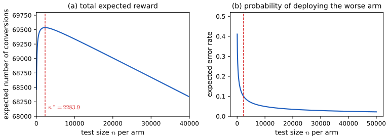
The figure matches the book: the reward rises sharply to its maximum at \(n^*=2284\) and decays slowly (the loss from overshooting by a given amount is less than half the loss from undershooting, gap 34.12), while the error rate keeps falling slowly beyond \(n^*\). One of the book's side remarks needs a correction. It says that the prior implies an expected effect size \(\E|\mu_1-\mu_0|=0.023\); for \(\mu_j\sim\N(m,\tau^2)\) independent, \(\mu_1-\mu_0\sim\N(0,2\tau^2)\) and \(\E|\mu_1-\mu_0|=2\tau/\sqrt\pi=0.034\) (0.023 is \(\E|\mu_j-m|=\tau\sqrt{2/\pi}\), the deviation of a single arm from the prior mean). The conclusion, that most changes have a tiny effect, stands.
34.4 Contextual bandits
p. 1120 (This section of the book is co-authored with Lihong Li.) An A/B test fixes the sizes \(n_0,n_1\) in advance. If the decision maker may react after every outcome the problem becomes sequential, and the simplest sequential decision problem is the bandit. The bandit regret demo runs the algorithms of this section side by side (preset 4 removes the exploration bonus, preset 5 explores too much).
34.4.1 Types of bandit
pp. 1120–1121 In a multi-armed bandit (MAB) an agent chooses an arm \(a_t\sim\pi_t\) and receives a reward \(r_t\sim p_R(\cdot\given a_t)\) with mean \(R(a)\). A contextual bandit adds a context \(s_t\) that evolves independently of the agent's actions, a policy \(\pi_t(a\given s_t)\) and a reward \(p_R(r\given s_t,a)\) with mean \(R(s,a)\). The data \(\mathcal D_{1:t}\), \(\mathcal D_t=(s_t,a_t,r_t)\) are used to update the policy while rewards keep accruing ("earning while learning"). The objective is the finite-horizon cumulative reward or its discounted infinite-horizon version, \[ J=\sum_{t=1}^T\E[r_t],\qquad J=\sum_{t=1}^\infty\gamma^{t-1}\E[r_t]. \tag{34.48, 34.49} \] The discount \(1-\gamma\) is the probability of termination at each step (gap 34.20). The book lists extensions: multiple plays (34.52, 34.53) and restless bandits, whose arm states evolve even when not pulled (34.54), and adversarial bandits (footnote 4). Only stochastic bandits are treated here.
34.4.2 Applications
p. 1122 In online advertising the context is the page, the action the ad shown and the reward a click (the click-through rate, CTR); in clinical trials the context is the patient, the action the treatment and the reward a cure. If the aim is only to find the best treatment as quickly as possible (not to maximise the reward during learning), the problem is best-arm identification (Audibert et al. 2010).
34.4.3 Exploration-exploitation tradeoff
p. 1122 To estimate \(R(s,a)\) the agent has to try actions (explore) before it can pick the apparent best (exploit). If it exploits a wrong model too early, it collects data from its own choices and reinforces the error, the feedback loop of Figure 34.7. This is unlike supervised learning, where data are drawn from a fixed distribution. The loop is made concrete in pml Section 22.4: a greedy policy has linear regret (gap 22.13), and the bandit feedback demo shows it.
34.4.4 The optimal solution
pp. 1122–1124 The posterior over the reward parameters given the history \(h_t=\{s_{1:t-1},a_{1:t-1},r_{1:t-1}\}\), \(b_t=p(\theta\given h_t)\), is the belief state (or information state); it is a finite sufficient statistic of the history and updates deterministically by Bayes' rule, \(b_t=\mathrm{BayesRule}(b_{t-1},a_t,r_t)\) (34.55). For a context-free Bernoulli bandit with factored Beta priors \(\prod_a\Beta(\mu_a\given\alpha_0^a,\beta_0^a)\) the posterior is \[ p(\theta\given\mathcal D_t)=\prod_a\Beta\big(\mu_a\given\alpha_0^a+N_t^0(a),\ \beta_0^a+N_t^1(a)\big),\qquad N_t^r(a)=\sum_{s<t}\ind(a_s=a,r_s=r) \tag{34.56–34.58} \] (the book's labelling of successes and failures in (34.57), \(\alpha\leftarrow N^0\), \(\beta\leftarrow N^1\), is swapped relative to its text: a success, \(r=1\), increases \(\alpha\); the arithmetic below uses the correct assignment). Figure 34.8 illustrates the updates of two arms; the book also lists the conjugate or approximate updates for Gaussian, linear-regression (Section 15.2), logistic-regression (15.3.5) and neural bandits (Chapter 17).
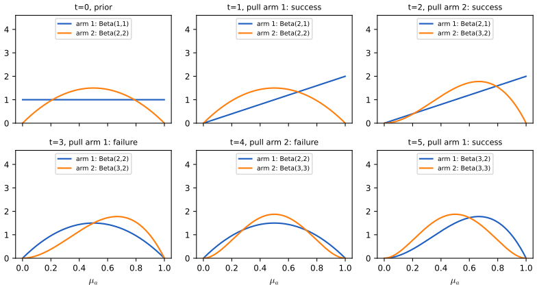
Writing the update as \(p(b_t\given b_{t-1},a_t,r_t)=\ind(b_t=\mathrm{BayesRule}(b_{t-1},a_t,r_t))\) (34.59) and predicting the reward by \(p(r_t\given b_t)=\int p_R(r_t\given s_t,a_t;\theta)p(\theta\given b_t)\d\theta\) (34.60) shows that the bandit is a (controlled) Markov decision process on belief states, the belief-state MDP. Its optimal policy is the Bayes-optimal exploration-exploitation trade-off; for a finite number of arms and a finite horizon it can be computed by dynamic programming, but the number of belief states grows polynomially in \(T\) with an exponent proportional to the number of arms, and for general contextual bandits the problem is intractable (Papadimitriou and Tsitsiklis 1987). Gap 34.15 carries out the dynamic programme for two arms, and Figure 34.23 shows how far from optimal the popular heuristics are at short horizons.
Filling the gap 34.15: the Beta posterior, the belief-state MDP and its exact solution pp. 1122–1124, (34.55)–(34.60)
Derivation
Posterior (34.57). The likelihood of the pulls of arm \(a\) is \(\prod\mu_a^{r_s}(1-\mu_a)^{1-r_s}=\mu_a^{s_a}(1-\mu_a)^{f_a}\) where \(s_a\) and \(f_a\) count successes and failures; with the independent priors \(\Beta(\alpha_0^a,\beta_0^a)\) the posterior factorises over arms and is \(\Beta(\alpha_0^a+s_a,\beta_0^a+f_a)\) (the conjugate update of Section 3.4.1, notes). Only the counts \((s_a,f_a)_a\) matter, not the order: the belief state is a finite sufficient statistic of the history. I confirmed the update against a numerically normalised posterior.
Why the belief-state MDP is exact. The distribution of the next reward given the whole history depends on the history only through \(b_t\) (34.60), and \(b_{t+1}\) is a deterministic function of \((b_t,a_t,r_t)\) (34.59). The expected total reward of a policy that is a function of the history is therefore the expected total reward of a policy that is a function of \(b_t\), and the optimal policy can be found by dynamic programming on belief states (gap 34.9).
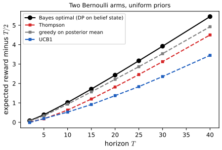
Two arms, finite horizon \(T\). Let \(V_t(s_1,f_1,s_2,f_2)\) be the optimal expected reward from step \(t\) on, with \(t=s_1+f_1+s_2+f_2\) pulls made, \(V_T=0\), posterior means \(\hat p_a=(\alpha_0^a+s_a)/(\alpha_0^a+\beta_0^a+s_a+f_a)\): \[ V_t=\max_a\ \Big[\hat p_a\big(1+V_{t+1}(\text{success of }a)\big)+(1-\hat p_a)V_{t+1}(\text{failure of }a)\Big]. \] For uniform priors, \(V_1=\tfrac12\) at the start (one pull, the arms are exchangeable). For \(T=2\), pull arm 1 (by symmetry): with probability \(\tfrac12\) it succeeds and its posterior mean becomes \(\tfrac23\), so one pulls it again; with probability \(\tfrac12\) it fails, its posterior mean drops to \(\tfrac13\) and the untouched arm 2 (mean \(\tfrac12\)) is better. So \(V=\tfrac12+\tfrac12\cdot\tfrac23+\tfrac12\cdot\tfrac12=\tfrac{13}{12}\), which the program reproduces exactly. For \(T=20\) the optimal value is \(12.431\), against \(T/2=10\) for a random arm: the gain over random is \(2.431\), compared with \(1.937\) for Thompson sampling, \(2.387\) for the greedy rule on the posterior mean and \(1.515\) for UCB1 (Monte Carlo over the prior, 20,000 runs; Figure 34.23). At short horizons exploring is expensive, which is why the greedy rule (with the prior doing the exploring) is hard to beat, and why UCB1, which explores on the scale of \(\sqrt{2\ln t}\), is wasteful. The state space has about \(T^4/24\) states for two arms; for \(K\) arms \(T^{2K}\), which is why the exact solution is used only as a benchmark.
Gittins index. For an infinite horizon with discount \(\gamma\) and independent arms, Gittins (1989) showed that the optimal policy plays the arm with the largest index, a number computed from that arm's belief alone; the book states this loosely ("a table of action probabilities"). I do not prove it here.
34.4.5 Upper confidence bounds (UCBs)
p. 1124 The optimal solution is intractable, so one uses "optimism in the face of uncertainty": act greedily on an optimistic estimate \(\tilde R_t(s,a)\ge R(s,a)\) that holds with high probability, \(a_t=\argmax_a\tilde R_t(s_t,a)\) (34.61). The bonus \(\tilde R_t-R\) shrinks as data accumulate, so exploration fades.
34.4.5.1 Frequentist approach
pp. 1124–1125 A concentration inequality gives \(|\hat R_t-R|\le\delta_t\) with high probability, and \(\tilde R_t=\hat R_t+\delta_t\). For a Bernoulli bandit with empirical mean \(\hat\mu_t(a)=N^1_t(a)/N_t(a)\) (34.62, 34.63), the Chernoff-Hoeffding inequality gives \[ \tilde R_t(a)=\hat\mu_t(a)+\frac{c}{\sqrt{N_t(a)}} \tag{34.64} \] for a constant \(c\) (gap 34.17 shows how \(c\) is tied to the confidence level; UCB1 uses \(c=\sqrt{2\ln t}\)).
34.4.5.2 Bayesian approach
p. 1125 With the Beta posterior the optimistic estimate is the posterior mean plus \(c\) posterior standard deviations, \[ \tilde R_t(a)=\hat\mu_t(a)+c\,\hat\sigma_t(a),\qquad\hat\sigma_t(a)\approx\sqrt{\frac{\hat\mu_t(a)(1-\hat\mu_t(a))}{N_t(a)}}, \tag{34.65, 34.66} \] with \(c\) controlling greediness. For a Gaussian bandit with an uninformative prior \(\hat\sigma_t(a)\) is the standard error of the mean.
Filling the gap 34.17: where the constant \(c\) comes from, and why the plug-in standard deviation (34.65) is unsafe pp. 1124–1125, (34.64)–(34.66)
Derivation
Hoeffding. For \(N\) independent rewards in \([0,1]\) with mean \(\mu\), \(\Pr(\hat\mu-\mu\ge\epsilon)\le e^{-2N\epsilon^2}\) and the same for the lower tail. Setting the right-hand side to \(p\) gives \(\epsilon=\sqrt{\ln(1/p)/(2N)}\), so \(\hat\mu+\sqrt{\ln(1/p)/(2N)}\ge\mu\) with probability at least \(1-p\): this is (34.64) with \(c=\sqrt{\ln(1/p)/2}\). A confidence level that tightens as time goes on is needed so that the optimistic bound is valid at every step simultaneously; taking \(p=t^{-4}\) gives \(c=\sqrt{2\ln t}\), the UCB1 index of Auer, Cesa-Bianchi and Fischer (2002). Its regret bound, \(\E N_T(a)\le8\ln T/\Delta_a^2+1+\pi^2/3\), is proved in pml gap 22.13; in a simulation of 200 runs with \(\mu=(0.7,0.4,0.3)\), \(T=3000\) the counts of the two suboptimal arms were 114 and 71, far below the bounds 716 and 405, so the bound holds with a lot of slack.
Plug-in standard deviation. The approximation (34.65) uses the empirical mean. If an arm has had only failures, \(\hat\mu=0\) and the plug-in standard deviation is exactly 0, so \(\tilde R=0\) however few pulls there were; if another arm has a positive index the first is never pulled again, and a lucky early run of failures can lock out the best arm. The exact standard deviation of the Beta posterior, \(\sqrt{\alpha\beta/((\alpha+\beta)^2(\alpha+\beta+1))}\) (with the prior counts included in \(\alpha,\beta\)), does not vanish, and is what my Bayes-UCB code uses. In my runs on the three-arm instance \(\mu=(0.7,0.4,0.3)\), a plug-in version with a floor of 0.01 on the standard deviation had mean regret about 61 at \(T=1000\), against 8.8 for the Beta-sd version and 43.7 for UCB1. The Bayesian bound is also not UCB1: its constant \(c\) has no guarantee in the same sense, and it works because it adapts to the posterior spread.
34.4.5.3 Example
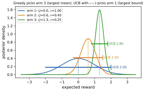
pp. 1125–1126 Figure 34.9 (from Silver 2018 in the book) illustrates the principle with three Gaussian arms: the posterior mean \(Q(a)\) and a bar \(c\hat\sigma(a)\) for each. The greedy rule picks the arm with the largest mean; UCB picks the arm with the largest upper end of its bar, which may be an arm that is poorly known.
34.4.6 Thompson sampling
p. 1126 Thompson sampling (probability matching) plays arm \(a\) with the probability that it is optimal, \[ \pi_t(a\given s_t,h_t)=p_a=\int\ind\Big(a=\argmax_{a'}R(s_t,a';\theta)\Big)p(\theta\given h_t)\d\theta, \tag{34.67} \] and one does not need to compute \(p_a\): draw a single posterior sample \(\tilde\theta_t\sim p(\theta\given h_t)\) and act greedily on it, \(a_t=\argmax_{a'}R(s_t,a';\tilde\theta_t)\) (34.68, 34.69). Uncertainty makes the sampled model vary, so many actions are tried; as the posterior concentrates, the policy exploits. Gap 34.18 proves that sample-then-exploit selects arm \(a\) with probability exactly \(p_a\).
Filling the gap 34.18: sample-then-exploit is probability matching p. 1126, (34.67)–(34.69)
Derivation
Let \(\tilde\theta\sim p(\theta\given h_t)\) and \(A=\argmax_{a'}R(s_t,a';\tilde\theta)\) (ties of probability zero or broken at random). The event \(\{A=a\}\) is a function of \(\tilde\theta\), so \(\Pr(A=a)=\int\ind(a=\argmax_{a'}R(s_t,a';\theta))p(\theta\given h_t)\d\theta=p_a\): the probability that \(a\) is optimal under the posterior, i.e. (34.69).
Beta-Bernoulli arms. With independent posteriors \(\Beta(\alpha_a,\beta_a)\), \(p_a=\int_0^1\mathrm{Beta}(x\given\alpha_a,\beta_a)\prod_{a'\ne a}F_{a'}(x)\d x\), with \(F_{a'}\) the Beta cdf (the arm \(a\) is optimal at \(x\) if all others are below it). For the three posteriors \(\Beta(3,2),\Beta(6,4),\Beta(2,5)\) this gives \(p=(0.4977,0.4698,0.0325)\), and \(6\times10^5\) sample-then-exploit draws select the arms with frequencies within \(0.004\) of these.
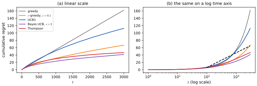
Regret. The book states that Thompson sampling has \(O(\sqrt{KT\log T})\) regret (Russo and Van Roy 2014). That bound is on the Bayesian regret (averaged over the prior), and I cite it without proof. The instance-dependent (frequentist) logarithmic regret of Thompson sampling for Bernoulli arms, which matches the lower bound of gap 34.19, is due to Kaufmann, Korda and Munos (2012) and Agrawal and Goyal (2012). In Figure 34.21 Thompson sampling has the smallest regret of the five algorithms at \(T=3000\) on the four-armed instance.
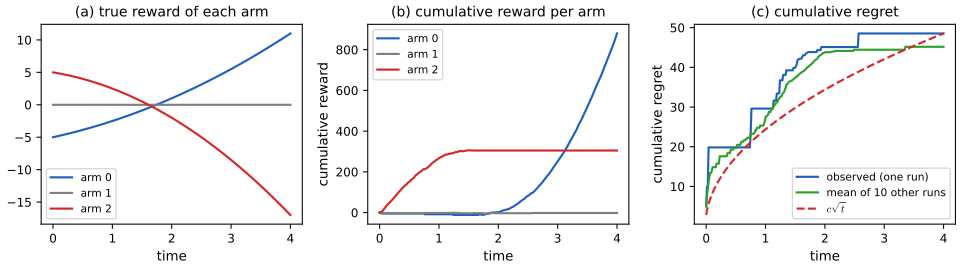
Figure 34.10 applies Thompson sampling to a linear regression bandit. The context is \(s_t=(1,t,t^2)\), the true mean reward of arm \(a\) is \(w_a^\T s_t\) with \(w_0=(-5,2,0.5)\), \(w_1=(0,0,0)\), \(w_2=(5,-1.5,-1)\) and noise variance 1: arm 0 starts bad and improves, arm 1 is useless, arm 2 starts good and decays. Each arm has a conjugate Gaussian-inverse-gamma prior and exact Bayesian updating (gap 34.16). The algorithm quickly abandons arm 1, first leans on arm 2 and then switches to arm 0 as the problem changes.
Filling the gap 34.16: the normal-inverse-gamma update behind Figure 34.10, and Thompson sampling with it p. 1126
Derivation
For one arm with observations \(y=\Phi w+\varepsilon\), \(\varepsilon\sim\N(0,\sigma^2I)\), take the prior \(w\given\sigma^2\sim\N(\mu_0,\sigma^2\Lambda_0^{-1})\), \(\sigma^2\sim\mathrm{IG}(a_0,b_0)\). The posterior is again of this form with \[ \Lambda_n=\Lambda_0+\Phi^\T\Phi,\quad\mu_n=\Lambda_n^{-1}(\Lambda_0\mu_0+\Phi^\T y),\quad a_n=a_0+\tfrac n2,\quad b_n=b_0+\tfrac12\big(y^\T y+\mu_0^\T\Lambda_0\mu_0-\mu_n^\T\Lambda_n\mu_n\big). \] This is derived by completing the square in \(w\) in gap 15.4. Two consequences used here: \(\mu_n\) is the ridge regression estimate with penalty matrix \(\Lambda_0\) (for \(\mu_0=0,\Lambda_0=I\): \((\Phi^\T\Phi+I)^{-1}\Phi^\T y\)), and \(b_n=b_0+\tfrac12\big(\|y-\Phi\mu_n\|^2+(\mu_n-\mu_0)^\T\Lambda_0(\mu_n-\mu_0)\big)\), the residual sum of squares plus the prior penalty. Both identities, and the formula for the log marginal likelihood \(-\tfrac n2\ln2\pi+\tfrac12\ln\tfrac{|\Lambda_0|}{|\Lambda_n|}+a_0\ln b_0-a_n\ln b_n+\ln\tfrac{\Gamma(a_n)}{\Gamma(a_0)}\), were confirmed numerically (the latter against a Monte Carlo average of the likelihood over the prior).
Thompson sampling step. Each arm keeps its own \((\mu_n,\Lambda_n,a_n,b_n)\), updated only when the arm is pulled. At time \(t\) draw \(\sigma^2_k\sim\mathrm{IG}(a_n,b_n)\) (the reciprocal of a gamma variable) and \(w_k\sim\N(\mu_n,\sigma^2_k\Lambda_n^{-1})\) for every arm, and pull the arm maximising \(w_k^\T s_t\). Because the prior is conjugate, a sample from the joint posterior is obtained exactly, in this order (variance first, weights given variance). In the run of the figure (\(T=300\) steps for \(t\in[0,4]\), prior \(\mu_0=0,\Lambda_0=I,a_0=b_0=1\)) arms 0, 1 and 2 were pulled 177, 19 and 104 times, and the cumulative regret ended at 48.5; averaged over six other runs the cumulative regret was 41.9 at \(t=2\) and 42.9 at \(t=4\), so almost all of it is incurred in the first half (the early exploration), as the flattening curve of the figure shows.
34.4.7 Regret
pp. 1127–1128 The per-step regret is the gap between the oracle's expected reward and the agent's, \(l_t=\E_{p(s_t)}[R(s_t,\pi^*(s_t))]-\E_{\pi_t p(s_t)}[R(s_t,a_t)]\) (34.70), and the cumulative (total) regret is \(L_T=\E\sum_{t\le T}l_t\) (34.71); the simple regret \(l_T\) matters only for pure exploration. Rewards bounded implies \(L_T=O(T)\); a policy that converges to the optimum has \(L_T=o(T)\). For a context-free bandit with gaps \(\Delta_a=R^*-R(a)\), \[ L_T=\E\sum_{t=1}^T\big(R^*-R(a_t)\big)=\sum_a\Delta_a\,\E[N_{T+1}(a)]. \tag{34.72} \] So under-exploration (stuck on a suboptimal arm) and over-exploration (pulling bad arms too often) both give linear regret, while UCB and Thompson sampling achieve sublinear regret. The decomposition (34.72) is proved, and the failure of greedy and fixed-\(\varepsilon\) policies shown, in pml gap 22.13 (the sum runs to \(T\); the book's \(N_{T+1}\) counts the pulls made through step \(T\)). The lower bound of Lai and Robbins (1985) for any reasonable algorithm is \[ \liminf_{T\to\infty}\frac{L_T}{\ln T}\ \ge\ \sum_{a:\Delta_a>0}\frac{\Delta_a}{\KL\big(p_R(a)\,\|\,p_R(a^*)\big)}, \tag{34.73} \] (the book writes the right side multiplied by \(\log T\) and drops the \(\liminf\) normalisation), so logarithmic regret is the best possible. Gap 34.19 proves it.
Filling the gap 34.19: the Lai-Robbins lower bound (34.73) p. 1128, (34.73)
Derivation
I prove it for Gaussian arms with known variance \(\sigma^2\) (so \(\KL(\N(\mu_a,\sigma^2)\|\N(\mu^*,\sigma^2))=\Delta_a^2/(2\sigma^2)\)); the Bernoulli case is the same with the Bernoulli KL divergence.
Setting. A policy is consistent if for every instance \(\mu\) and every \(p>0\), \(R_T(\mu)=o(T^p)\), where \(R_T\) is the expected regret (policies such as fixed-\(\varepsilon\) greedy, with linear regret, are excluded: that is why they can beat the bound at moderate \(T\)). Claim: for every suboptimal arm \(a\), \(\liminf_T\E[N_a(T)]/\ln T\ge2\sigma^2/\Delta_a^2\). Summing \(\Delta_a\E N_a\) over arms gives (34.73): \(\sum_a2\sigma^2/\Delta_a=\sum_a\Delta_a/\KL\).
Proof (the standard change-of-measure argument of Lai and Robbins 1985, in the form given by Lattimore and Szepesvári 2020). Fix a suboptimal arm \(a\) and \(\varepsilon>0\); let \(\mu'\) equal \(\mu\) except \(\mu'_a=\mu^*+\varepsilon\), so \(a\) is the unique best arm of \(\mu'\), with every other arm at least \(\varepsilon\) worse. Let \(P,P'\) be the laws of the history (actions and rewards up to \(T\)) under \(\mu,\mu'\).
(i) Divergence decomposition. By the chain rule of the KL divergence over the sequential interaction (the policy's conditional distributions are the same under both, so they cancel), \(\KL(P\|P')=\E_P[N_a(T)]\cdot\KL(\mu_a,\mu'_a)=\E_P[N_a(T)]\,(\Delta_a+\varepsilon)^2/(2\sigma^2)\), because only arm \(a\) differs.
(ii) Bretagnolle-Huber inequality. For every event \(A\), \(P(A)+P'(A^c)\ge\tfrac12e^{-\KL(P\|P')}\).
(iii) Regret on the event \(A=\{N_a(T)>T/2\}\). Under \(\mu\) every pull of \(a\) costs \(\Delta_a\), so \(R_T(\mu)\ge\Delta_a\tfrac T2P(A)\). Under \(\mu'\), on \(A^c\) at least \(T/2\) pulls are of arms costing at least \(\varepsilon\), so \(R_T(\mu')\ge\varepsilon\tfrac T2P'(A^c)\). With \(\kappa=\min(\Delta_a,\varepsilon)\): \(P(A)+P'(A^c)\le2(R_T(\mu)+R_T(\mu'))/(\kappa T)\).
Combining (ii) and (iii) and taking logarithms, \[ \KL(P\|P')\ \ge\ \ln\frac{\kappa T}{4\,(R_T(\mu)+R_T(\mu'))}. \] Divide by \(\ln T\). Consistency gives \(\ln(R_T(\mu)+R_T(\mu'))/\ln T\le p\) eventually for every \(p>0\), so \(\liminf_T\KL(P\|P')/\ln T\ge1\), i.e. \(\liminf\E_P[N_a(T)]/\ln T\ge2\sigma^2/(\Delta_a+\varepsilon)^2\). Let \(\varepsilon\downarrow0\). \(\square\)
Bernoulli arms. The same argument with the alternative \(\mu'_a\) slightly above \(\mu^*\) gives the constant \(\Delta_a/\KL(\mathrm{Ber}(\mu_a)\|\mathrm{Ber}(\mu^*))\). For \(\mu=(0.5,0.45,0.4,0.3)\) it is \(9.98+4.90+2.43=17.38\) per unit of \(\ln T\) (the instance of Figure 34.21). It is an asymptotic statement: at \(T=3000\) the simulated Thompson regret, 47 (Figure 34.21), is still below \(17.38\ln3000=139\), as an average-case finite-horizon curve may be. The UCB1 bound is a constant factor larger than the lower bound (for Bernoulli arms \(\sigma^2\le\tfrac14\), so \(2\sigma^2\le\tfrac12\), against 8), which explains why Bayesian UCB and Thompson sampling beat UCB1 in practice.
34.5 Markov decision problems
p. 1128 In a bandit the context does not respond to the agent's actions. Letting the state of the world change with the action gives a Markov decision process (MDP), the foundation of reinforcement learning (Chapter 35). The value iteration demo lets you build a grid world and watch the planning algorithms of Section 34.6.
34.5.1 Basics
pp. 1128–1129 An MDP is a tuple \(\langle\mathcal S,\mathcal A,p,p_R,p_0\rangle\): states, actions, a transition model \(p(s'\given s,a)\), a reward model and an initial distribution. At time \(t\) the agent sees \(s_t\), takes \(a_t\sim\pi(\cdot\given s_t)\) and the environment returns \(r_t\sim p_R(\cdot\given s_t,a_t,s_{t+1})\) and the next state. A trajectory \(\tau\) of length \(T\) has probability \[ p(\tau)=p_0(s_0)\prod_{t=0}^{T-1}\pi(a_t\given s_t)\,p(s_{t+1}\given s_t,a_t)\,p_R(r_t\given s_t,a_t,s_{t+1}), \tag{34.74} \] and only the mean reward matters for expected total reward, \(R(s,a)=\E_{p(s'\given s,a)}\E_{p_R}[r]\) (34.75), so one writes \(\langle\mathcal S,\mathcal A,p,R,p_0\rangle\). With finite sets the model is a table (a finite state machine, Figure 34.11, a drawing and not reproduced). Control theory uses different names (plant, controller, cost) for the same objects.
34.5.2 Partially observed MDPs
p. 1130 If the agent sees only a noisy observation \(o_t\sim p(\cdot\given s_t,a_t)\) of the hidden state it faces a partially observable MDP (POMDP, Figure 34.12). The policy maps the history \(h_t=(a_1,o_1,\dots,a_{t-1},o_t)\) to actions. The optimal solution tracks the belief state \(b_t=p(s_t\given h_t)\) and treats it as the state of a belief-state MDP, which is intractable in general; a common approximation feeds the last \(k\) observations to the policy as if they were the state. Gap 34.23 derives the belief update and shows why the belief-state value function has a simple shape.
Filling the gap 34.23: the belief update of a POMDP and the piecewise-linear value function p. 1130
Derivation
Belief update. After action \(a\) and observation \(o'\), by Bayes' rule and the Markov property, \[ b'(s')=p(s'\given h,a,o')=\frac{p(o'\given s',a)\sum_sp(s'\given s,a)b(s)}{p(o'\given b,a)},\qquad p(o'\given b,a)=\sum_{s'}p(o'\given s',a)\sum_sp(s'\given s,a)b(s). \] The new belief is a deterministic function of \((b,a,o')\), and \(o'\) occurs with probability \(p(o'\given b,a)\): this is the dynamics of the belief-state MDP, with reward \(R(b,a)=\sum_sb(s)R(s,a)\). I checked the update against brute-force conditioning of the joint distribution on a two-state example.
Piecewise-linear convexity (finite horizon). Suppose \(V_{t+1}(b)=\max_{\alpha\in\Gamma_{t+1}}\alpha^\T b\) for a finite set of vectors \(\Gamma_{t+1}\) (true for \(V_T\equiv0\)). The key identity is that the unnormalised new belief is linear in \(b\): \(p(o'\given b,a)\,b'(s')=\sum_sb(s)\,p(o'\given s',a)p(s'\given s,a)\). Hence \(p(o'\given b,a)V_{t+1}(b')=\max_\alpha\sum_sb(s)g_{a,o',\alpha}(s)\) with \(g_{a,o',\alpha}(s)=\sum_{s'}p(o'\given s',a)p(s'\given s,a)\alpha(s')\) (the maximum commutes with the positive factor \(p(o'\given b,a)\)). Then \[ V_t(b)=\max_a\Big[\sum_sb(s)R(s,a)+\gamma\sum_{o'}\max_\alpha b^\T g_{a,o',\alpha}\Big] \] is again a maximum of finitely many linear functions of \(b\). So the optimal value function is convex and piecewise linear in the belief, though the number of vectors may grow exponentially with the horizon, which is why exact POMDP planning is hard.
34.5.3 Episodes and returns
pp. 1130–1131 A task that can go on forever is continuing; an episodic task ends in an absorbing state (one that returns to itself with reward 0), after which a new episode may start from \(p_0\); a fixed known length gives a finite-horizon problem. The return from time \(t\) is the discounted reward-to-go, \[ G_t=r_t+\gamma r_{t+1}+\dots=\sum_{k\ge0}\gamma^kr_{t+k},\qquad G_t=r_t+\gamma G_{t+1}. \tag{34.76–34.78} \] The discount keeps the return finite when \(T=\infty\) (for bounded rewards \(|G_t|\le r_{\max}/(1-\gamma)\)) and favours near-term reward; \(\gamma=0\) is myopic. It can also be read as the probability \(1-\gamma\) that the interaction ends at each step (gap 34.20).
34.5.4 Value functions
p. 1131 For a policy \(\pi\) the state-value function, the action-value (Q) function and the advantage function are \[ V_\pi(s)=\E_\pi[G_0\given s_0=s],\quad Q_\pi(s,a)=\E_\pi[G_0\given s_0=s,a_0=a],\quad A_\pi(s,a)=Q_\pi(s,a)-V_\pi(s), \tag{34.79–34.81} \] and \(V_\pi(s)=\E_{\pi(a\given s)}Q_\pi(s,a)\), so the advantage has mean zero under \(\pi\).
Filling the gap 34.20: returns, the discount as a termination probability, and the Bellman expectation equations pp. 1121, 1130–1132, (34.49), (34.76)–(34.81)
Derivation
Recursion (34.78). \(G_t=\sum_{k\ge0}\gamma^kr_{t+k}=r_t+\gamma\sum_{k\ge0}\gamma^kr_{t+1+k}=r_t+\gamma G_{t+1}\).
Discounting is termination (34.49). Let \(\tau\) be independent of everything, with \(\Pr(\tau>t)=\gamma^t\) (the agent survives each step with probability \(\gamma\)); then the undiscounted reward collected before termination has expectation \(\E\sum_{t<\tau}r_t=\sum_t\Pr(\tau>t)\E r_t=\sum_t\gamma^t\E r_t\), which is the discounted sum. A simulation with \(\gamma=0.9\) confirms 1.152 against 1.153 (a fixed reward sequence, \(4\times10^5\) geometric lifetimes). The expected lifetime is \(1/(1-\gamma)\) steps, the effective horizon.
Bellman expectation equations. Condition on the first step: \(Q_\pi(s,a)=\E[r_0+\gamma G_1\given s_0=s,a_0=a]=R(s,a)+\gamma\sum_{s'}p(s'\given s,a)V_\pi(s')\), since given \(s_1\) the future return does not depend on \((s_0,a_0)\) (Markov property) and has mean \(V_\pi(s_1)\). Averaging over \(a\sim\pi(\cdot\given s)\) gives \(V_\pi(s)=\sum_a\pi(a\given s)Q_\pi(s,a)\) and hence \(\E_{a\sim\pi}A_\pi(s,a)=V_\pi(s)-V_\pi(s)=0\). In vector form, \(v=r_\pi+\gamma T_\pi v\) (34.88, next section).
34.5.5 Optimal value functions and policies
p. 1132 A policy is optimal if \(V_{\pi^*}\ge V_\pi\) in every state for all \(\pi\); the optimal value functions \(V_*,Q_*\) are unique even if the optimal policy is not, and every finite MDP has a deterministic optimal policy (Puterman 1994). Bellman's optimality equations are \[ V_*(s)=\max_a\Big[R(s,a)+\gamma\E_{p(s'\given s,a)}V_*(s')\Big],\qquad Q_*(s,a)=R(s,a)+\gamma\E_{p(s'\given s,a)}\Big[\max_{a'}Q_*(s',a')\Big], \tag{34.82, 34.83} \] and the optimal policy is the greedy policy \(\pi_*(s)=\argmax_aQ_*(s,a)=\argmax_a[R(s,a)+\gamma\E V_*(s')]\) (34.84, 34.85). The gap between the two sides of (34.82), (34.83) for an arbitrary candidate \(V\) or \(Q\) is the Bellman error (residual). Evaluating a given policy replaces \(\max_a\) by \(\E_{\pi(a\given s)}\). The book also mentions how to take the maximum over a continuous action: optimising one dimension at a time, the cross-entropy method, mixed-integer programming for ReLU networks, or amortising it with a trained policy.
Filling the gap 34.21: Bellman's optimality equations, uniqueness, the contraction and a deterministic optimal policy pp. 1132, 1134, (34.82)–(34.87)
Derivation
Operators. For a policy \(\pi\) define \((T_\pi V)(s)=\sum_a\pi(a\given s)[R(s,a)+\gamma\sum_{s'}p(s'\given s,a)V(s')]\) and \((T^*V)(s)=\max_a[R(s,a)+\gamma\sum_{s'}p(s'\given s,a)V(s')]\). Both are monotone (\(V\le W\Rightarrow TV\le TW\), because the weights \(p\) are nonnegative) and are \(\gamma\)-contractions in the sup norm \(\|\cdot\|_\infty\): for \(T_\pi\), \(|T_\pi V-T_\pi W|(s)\le\gamma\sum_{a,s'}\pi\,p\,|V-W|(s')\le\gamma\|V-W\|_\infty\); for \(T^*\), use \(|\max_ax_a-\max_ay_a|\le\max_a|x_a-y_a|\) and the same bound. This is (34.87): \(\|V_{k+1}-V_*\|_\infty\le\gamma\|V_k-V_*\|_\infty\) once \(V_*\) is known to be the fixed point.
Existence and uniqueness of a fixed point. By Banach's fixed-point theorem, \(T^*\) has a unique fixed point \(\bar V\), the only solution of (34.82), and \(T_\pi\) has a unique fixed point, which is \(V_\pi\) (it satisfies the Bellman expectation equation of gap 34.20).
The fixed point is the optimal value. Let \(\bar\pi\) be greedy for \(\bar V\), i.e. \(T_{\bar\pi}\bar V=T^*\bar V=\bar V\). Then \(\bar V\) is the fixed point of \(T_{\bar\pi}\), so \(\bar V=V_{\bar\pi}\). For any policy \(\pi\) (even stochastic or history-dependent Markov), \(T_\pi\bar V\le T^*\bar V=\bar V\); applying the monotone \(T_\pi\) repeatedly, \(T_\pi^k\bar V\le\bar V\), and \(T_\pi^k\bar V\to V_\pi\) by contraction. So \(V_\pi\le\bar V=V_{\bar\pi}\) for all \(\pi\): \(\bar\pi\) is optimal, \(V_*=\bar V\), and a deterministic optimal policy exists. The same argument for the operator on \(Q\) gives (34.83), and the greedy policy extraction (34.84, 34.85): it is the \(\bar\pi\) above, with \(\max_aQ_*(s,a)=V_*(s)\). "The only solutions" in the book is the uniqueness statement just proved.
Bellman error controls value error. For any \(V\), \(\|V-V_*\|\le\|V-T^*V\|+\|T^*V-T^*V_*\|\le\|V-T^*V\|+\gamma\|V-V_*\|\), so \(\|V-V_*\|_\infty\le\|V-T^*V\|_\infty/(1-\gamma)\): a small Bellman residual implies a near-optimal value, and the constant blows up as \(\gamma\to1\).
34.5.5.1 Example
p. 1133 Figure 34.13 shows a one-dimensional grid world with absorbing end states \(S_{T1},S_{T2}\), three interior states, the actions up and down and reward 1 on entering \(S_{T2}\). The optimal \(Q_*\) depends on \(\gamma\): at \(\gamma=0\) only the last move counts, at \(\gamma=1\) the position does not matter, at \(\gamma=0.9\) shorter paths are better.
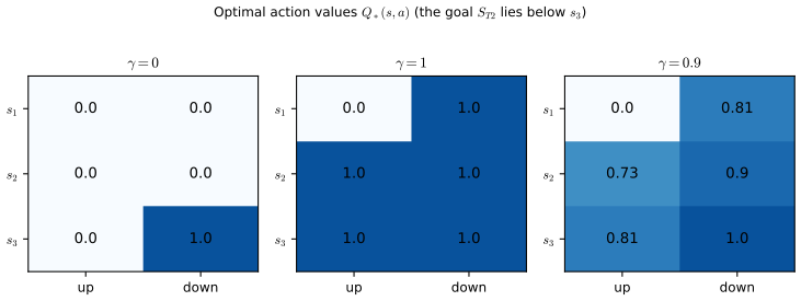
Filling the gap 34.22: closed form of \(Q_*\) in the grid world, and a slip at \(\gamma=1\) p. 1133, Figure 34.13
Derivation
Moves are deterministic. From \(s_k\) (\(k=1,2,3\), counted from the top) moving down reaches \(S_{T2}\) after \(4-k\) moves, the last of which yields the reward 1, so the best path from \(s_k\) has value \(V_*(s_k)=\gamma^{3-k}\) (the reward arrives at step \(3-k\) counting from 0). Then \[ Q_*(s_k,\text{down})=\gamma^{3-k}\ (k=1,2,3),\quad Q_*(s_k,\text{up})=\gamma V_*(s_{k-1})=\gamma^{5-k}\ (k=2,3),\quad Q_*(s_1,\text{up})=0, \] since moving up from \(s_1\) enters the absorbing state \(S_{T1}\) with reward 0. For \(\gamma=0.9\): \(0.81,0.9,1.0\) (down) and \(0,0.729,0.81\) (up), the numbers in the figure (the book rounds 0.729 to 0.73). For \(\gamma=0\) (with \(0^0=1\)) only \(Q_*(s_3,\text{down})=1\) is nonzero. For \(\gamma=1\), \(Q_*=1\) everywhere except \((s_1,\text{up})\), where it is 0.
The slip. The text says that at \(\gamma=1\) "\(Q_*(s,a)=1\) for all state-action pairs since the agent can always reach the goal eventually"; the figure itself (and the formula) show \(0\) for \((s_1,\text{up})\): that action ends the episode at \(S_{T1}\). The book's remark that at \(\gamma=1\) the Q-values give no short-term guidance is right for \(s_2,s_3\), where both actions are optimal (tied at 1), so the optimal policy is not unique at \(\gamma=1\). I confirmed these Q-tables by value iteration.
34.6 Planning in an MDP
p. 1134 Planning computes an optimal policy when the model is known; learning when it is not is reinforcement learning (Chapter 35). The methods are dynamic programming and linear programming. Their cost grows polynomially in \(|\mathcal S|\) and \(|\mathcal A|\), which is prohibitive when the state space is a product (the curse of dimensionality); approximate dynamic programming then represents values or policies parametrically.
34.6.1 Value iteration
pp. 1134–1135 Value iteration starts from any \(V_0\) and applies the Bellman backup \[ V_{k+1}(s)=\max_a\Big[R(s,a)+\gamma\sum_{s'}p(s'\given s,a)V_k(s')\Big], \tag{34.86} \] which is a contraction, \(\max_s|V_{k+1}(s)-V_*(s)|\le\gamma\max_s|V_k(s)-V_*(s)|\) (34.87), so \(V_k\to V_*\) geometrically and the greedy policy can be read off. It can be run on \(Q\) instead. For shortest-path problems one may care only about the states reachable from a start state; real-time dynamic programming (RTDP; Barto, Bradtke and Singh 1995) backs up the current state, acts, and repeats, an asynchronous form of value iteration that concentrates effort where the agent goes. Gap 34.24 proves the rate and a stopping rule for the policy. In the demo, preset 3, the error follows the dotted \(\gamma^k\) line, and preset 4 shows how slowly \(\gamma=0.99\) contracts.
Filling the gap 34.24: the rate of value iteration, a stopping rule, and the quality of the greedy policy pp. 1134–1135, (34.86), (34.87)
Derivation
Rate. \(V_*\) is the fixed point of \(T^*\) (gap 34.21), so \(\|V_k-V_*\|=\|T^*V_{k-1}-T^*V_*\|\le\gamma\|V_{k-1}-V_*\|\), hence \(\|V_k-V_*\|\le\gamma^k\|V_0-V_*\|\). To reach accuracy \(\epsilon\) takes \(k\ge\ln(\|V_0-V_*\|/\epsilon)/\ln(1/\gamma)\approx\ln(\cdot)/(1-\gamma)\) iterations, so the cost is \(O(|\mathcal S|^2|\mathcal A|)\) per sweep and a number of sweeps proportional to the effective horizon.
A computable stopping rule. Let \(\delta_k=\|V_k-V_{k-1}\|\). Then \(\|V_k-V_*\|\le\sum_{j\ge1}\|V_{k+j}-V_{k+j-1}\|\le\sum_{j\ge1}\gamma^j\delta_k=\frac{\gamma}{1-\gamma}\delta_k\). Let \(\pi\) be greedy for \(V=V_{k-1}\), so \(T_\pi V=T^*V=V_k\). Since \(V_\pi\) is the fixed point of the \(\gamma\)-contraction \(T_\pi\), \(\|V_\pi-V\|\le\|T_\pi V-V\|/(1-\gamma)=\delta_k/(1-\gamma)\); with \(\|V-V_*\|\le\|T^*V-V\|/(1-\gamma)\) from gap 34.21, \[ \|V_\pi-V_*\|_\infty\le\frac{2\,\delta_k}{1-\gamma}. \] So stop when \(\delta_k\le\epsilon(1-\gamma)/2\): the greedy policy is then \(\epsilon\)-optimal, even though \(V_k\) itself need not be that close. Checked on 40 random MDPs (6 states, 3 actions, \(\gamma=0.9\)): the contraction at every sweep, the stopping bound, and a zero Bellman residual at convergence.
Asynchronous updates. Updating one state at a time with the latest values (Gauss-Seidel, or RTDP) converges when every state is updated infinitely often, because each update is monotone and nonexpansive in the sup norm; I do not prove it here.
34.6.2 Policy iteration
pp. 1135–1136 Policy iteration alternates policy evaluation and policy improvement over deterministic policies. With \(v=V_\pi\), \(r(s)=\sum_a\pi(a\given s)R(s,a)\) and \(T(s'\given s)=\sum_a\pi(a\given s)p(s'\given s,a)\), the Bellman equation is the linear system \[ v=r+\gamma Tv,\qquad v=(I-\gamma T)^{-1}r \tag{34.88} \] (or iterate \(v_{t+1}=r+\gamma Tv_t\)). The improvement step takes the greedy policy \(\pi'(s)=\argmax_a\{R(s,a)+\gamma\E V_\pi(s')\}\), and \(V_{\pi'}\ge V_\pi\): from \(r'+\gamma T'v\ge r+\gamma Tv=v\) one iterates \[ v\le r'+\gamma T'v\le r'+\gamma T'(r'+\gamma T'v)\le\dots=(I-\gamma T')^{-1}r'=v' \tag{34.89, 34.90} \] (the book writes \(r\) instead of \(r'\) in the last expression; the Neumann series is applied to \(r'\)). The sequence \(\pi_0\overset E\to V_{\pi_0}\overset I\to\pi_1\overset E\to\dots\overset I\to\pi_*\overset E\to V_*\) (34.91) stops when the policy is greedy for its own value, which implies optimality; there are at most \(|\mathcal A|^{|\mathcal S|}\) deterministic policies and every iteration strictly improves, so it terminates. Value iteration is one evaluation sweep followed by an improvement (the max); generalised policy iteration (GPI) intermixes the two freely. The book's policy improvement theorem (Sutton and Barto 2018): if \(Q_\pi(s,\pi'(s))\ge V_\pi(s)\) for all \(s\), then \(V_{\pi'}\ge V_\pi\). Gap 34.25 proves all of this.
Filling the gap 34.25: policy evaluation, the policy improvement theorem and finite termination pp. 1135–1136, (34.88)–(34.91)
Derivation
Evaluation (34.88). \(T\) is a stochastic matrix (nonnegative, rows sum to 1), so its spectral radius is at most 1 and that of \(\gamma T\) at most \(\gamma<1\). Hence \(I-\gamma T\) is invertible and \((I-\gamma T)^{-1}=\sum_{k\ge0}(\gamma T)^k\) (Neumann series; I checked the sum numerically). It is a nonnegative matrix with \((I-\gamma T)^{-1}\ge I\), and \(v=(I-\gamma T)^{-1}r\) is the unique solution of \(v=r+\gamma Tv\).
Improvement theorem. Let \(\pi'\) satisfy \(T_{\pi'}V_\pi\ge V_\pi\) componentwise, which is the statement \(Q_\pi(s,\pi'(s))\ge V_\pi(s)\) for all \(s\) (and holds for the greedy \(\pi'\) because \(T_{\pi'}V_\pi=T^*V_\pi\ge T_\pi V_\pi=V_\pi\)). By monotonicity of \(T_{\pi'}\), \(T_{\pi'}^{k+1}V_\pi\ge T_{\pi'}^kV_\pi\ge\dots\ge V_\pi\) for every \(k\), and \(T_{\pi'}^kV_\pi\to V_{\pi'}\) by contraction, so \(V_{\pi'}\ge V_\pi\). In matrix form this is (34.89, 34.90): with \(n\) steps, \(v\le\sum_{k<n}(\gamma T')^kr'+(\gamma T')^nv\to(I-\gamma T')^{-1}r'=v'\).
Strict improvement. Let \(w=r'+\gamma T'v-v\ge0\). Then \(v'-v=(I-\gamma T')^{-1}w\ge w\) (since \((I-\gamma T')^{-1}\ge I\)), so if \(w(s)>0\) at some state then \(v'(s)>v(s)\). For the greedy \(\pi'\) with a change of action at \(s\), \(w(s)>0\).
Termination and optimality. If the greedy policy equals \(\pi\) (up to ties), then \(T^*V_\pi=T_\pi V_\pi=V_\pi\), so \(V_\pi\) is the fixed point of \(T^*\), i.e. \(V_*\) (gap 34.21). Otherwise the new policy has a value that is weakly larger everywhere and strictly larger somewhere, so no deterministic policy is visited twice, and the iteration stops after at most \(|\mathcal A|^{|\mathcal S|}\) improvements. In practice the number of sweeps is tiny: on the stochastic \(4\times4\) grid world below, policy iteration needs 4, 5 and 6 sweeps for \(\gamma=0.5,0.9,0.99\), value iteration (to \(10^{-10}\)) 21, 38 and 46. Each policy iteration sweep costs a linear solve, \(O(|\mathcal S|^3)\), so which is faster depends on the size of the problem. Checked on 40 random MDPs: the values \(V_{\pi_k}\) increase monotonically and end at \(V_*\), the same as value iteration.
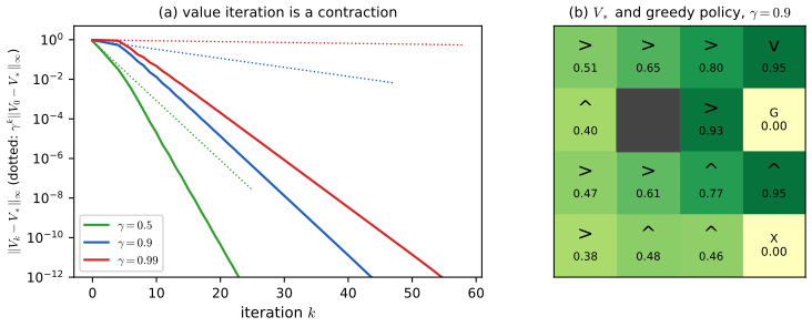
34.6.3 Linear programming
pp. 1136–1137 Linear programming (LP) is an alternative that is used for off-policy RL (Section 35.5). With \(p_0(s)>0\) the primal LP is \[ \min_V\sum_sp_0(s)V(s)\quad\text{s.t.}\quad V(s)\ge R(s,a)+\gamma\sum_{s'}p(s'\given s,a)V(s')\ \ \forall(s,a) \tag{34.92} \] (the book prints \(V(s)\) in the sum over \(s'\); it must be \(V(s')\)). Any feasible \(V\) satisfies \(V\ge V_*\), and the minimiser is \(V_*\); an action that makes the constraint tight in a state is optimal there. The dual, over nonnegative \(d(s,a)\), is \[ \max_{d\ge0}\sum_{s,a}d(s,a)R(s,a)\quad\text{s.t.}\quad\sum_ad(s,a)=(1-\gamma)p_0(s)+\gamma\sum_{\bar s,\bar a}p(s\given\bar s,\bar a)d(\bar s,\bar a), \tag{34.93} \] where feasible \(d\) are the normalised occupancy distributions of policies \(\pi_d(a\given s)=d(s,a)/\sum_{a'}d(s,a')\), \[ d(s,a)=(1-\gamma)\sum_{t\ge0}\gamma^t\Pr(s_t=s,a_t=a\given s_0\sim p_0,\ a_t\sim\pi_d(s_t)), \tag{34.94} \] and the objective is the average per-step reward under that occupancy. The LPs have as many constraints or variables as state-action pairs, so approximations (parametrised variables, sampled constraints) are needed at scale. Gap 34.26 proves the statements.
Filling the gap 34.26: the primal and dual linear programs of an MDP pp. 1136–1137, (34.92)–(34.94)
Derivation
Feasible \(V\) are optimistic. The constraints say \(V\ge R(s,a)+\gamma\sum p\,V=:(T_aV)(s)\) for every \(a\), i.e. \(V\ge T^*V\). By monotonicity \(V\ge T^*V\ge(T^*)^2V\ge\dots\to V_*\), so \(V\ge V_*\). \(V_*\) itself is feasible (it satisfies (34.82) with equality for the maximising actions and with \(\ge\) for the others). So \(V_*\) is the componentwise smallest feasible vector, and for \(p_0>0\) every other feasible \(V\) has \(p_0^\T V>p_0^\T V_*\): the LP has the unique solution \(V_*\). In a state \(s\) where the constraint for \(a\) is tight, \(V_*(s)=R(s,a)+\gamma\E V_*(s')\), so \(a\) is greedy, hence optimal.
The dual. Introduce multipliers \(d(s,a)\ge0\) for the constraints: \(\mathcal L(V,d)=\sum_sp_0(s)V(s)+\sum_{s,a}d(s,a)\big[R(s,a)+\gamma\sum_{s'}p(s'\given s,a)V(s')-V(s)\big]\). Minimising over the unconstrained \(V\) gives \(-\infty\) unless the coefficient of every \(V(s')\) vanishes: \(p_0(s')+\gamma\sum_{s,a}d(s,a)p(s'\given s,a)-\sum_ad(s',a)=0\), in which case the minimum is \(\sum d(s,a)R(s,a)\). Rescaling \(d\mapsto(1-\gamma)d\) turns the constraint into (34.93) and the objective into \((1-\gamma)\sum dR\). Strong duality for a feasible bounded LP gives \[ \max_{d\text{ feasible for (34.93)}}\sum d\,R=(1-\gamma)\,p_0^\T V_*. \] Occupancy measures. For a policy \(\pi\) with occupancy (34.94), \(\sum_ad(s,a)=(1-\gamma)\sum_t\gamma^t\Pr(s_t=s)=(1-\gamma)p_0(s)+\gamma(1-\gamma)\sum_{t\ge0}\gamma^t\Pr(s_{t+1}=s)=(1-\gamma)p_0(s)+\gamma\sum_{\bar s,\bar a}p(s\given\bar s,\bar a)d(\bar s,\bar a)\), which is the constraint of (34.93). Conversely, for a nonnegative \(d\) satisfying it, the state marginal \(x(s)=\sum_ad(s,a)\) solves \((I-\gamma T_{\pi_d}^\T)x=(1-\gamma)p_0\), whose unique solution is \(x=(1-\gamma)\sum_t\gamma^t(T_{\pi_d}^\T)^tp_0\), the discounted state occupancy of \(\pi_d\); so \(d\) is the occupancy of \(\pi_d\) on the states it visits (footnote 6: where \(x(s)=0\) the policy is arbitrary). The objective \(\sum dR=\sum_s x(s)\sum_a\pi_d(a\given s)R(s,a)=(1-\gamma)p_0^\T V_{\pi_d}\), so maximising it maximises the expected discounted return, and \(\pi_*(a\given s)=d^*(s,a)/\sum_{a'}d^*(s,a')\) is optimal.
Numerical agreement. On the stochastic \(4\times4\) grid world (15 states, 4 actions, \(\gamma=0.9\), \(p_0\) uniform), solving both LPs with a standard solver gives: the primal solution equals \(V_*\) from value iteration to \(10^{-7}\), the primal objective is \(0.5587\), the dual objective is \(0.05587=(1-\gamma)\cdot0.5587\), and the policy read off the dual occupancy attains \(V_*\) on every visited state. Value iteration, policy iteration and the two LPs are four routes to the same \(V_*\).
34.7 Active learning
p. 1137 (This section of the book is co-authored with Zeel B Patel.) In active learning (AL) the agent chooses which data to label, aiming to learn a predictive function from as few labels as possible; this is valuable when labels are expensive, as in medical imaging. The book reviews a few methods; the introductory volume has a parallel treatment (pml Section 19.4, with the active-learning demo). Figure 34.15 shows the effect for a logistic regression on a simulated two-dimensional, three-class problem: after 11 extra labels the model trained on margin-sampled points is more accurate than the model trained on random ones.
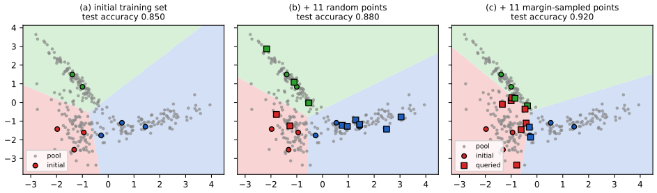
34.7.1 Active learning scenarios
p. 1138 Three settings: membership query synthesis (the agent may generate any input and ask for its label, Angluin 1988; mostly theoretical because generative models and instant oracles are rare), stream-based selective sampling (inputs arrive one by one and the agent decides whether to buy the label, Atlas, Cohn and Ladner 1989) and pool-based sampling (a pool of unlabelled inputs is available and an acquisition function ranks candidates, Lewis and Gale 1994). The rest of the section is pool-based.
34.7.2 Relationship to other forms of sequential decision making
pp. 1138–1139 Active learning, Bayesian optimisation (BO, Section 6.6, notes) and contextual bandits differ in the quantity they optimise, summarised here in my own words.
| Problem | Goal | What the agent chooses |
|---|---|---|
| Active learning | find a function \(f\) with small expected loss over random inputs, \(\min_f\E_{p(x)}\ell(f^*(x),f(x))\) | the input \(x\) whose label \(y=f^*(x)\) is bought |
| Bayesian optimisation | find an input maximising the unknown function, \(\max_xf^*(x)\) | the input \(x\) at which \(f^*\) is evaluated |
| Contextual bandit | find a policy maximising expected reward, \(\max_\pi\E_{p(x)\pi(a\given x)}R^*(x,a)\) | the action \(a\) (the context \(x\) is given, not chosen) |
(Table 34.1.) In each case the agent faces an exploration-exploitation trade-off and can model its uncertainty with, for example, a Gaussian process (Chapter 18) and an acquisition function \(\alpha(x)\), choosing \(x_{t+1}=\argmax_x\alpha(x)\). For AL regression a natural \(\alpha\) is the predictive variance; for BO, the probability of improvement (gap 6.21). The first makes the agent query "all over the place", the second makes it zoom in, as in Figure 34.16.
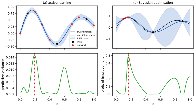
34.7.3 Acquisition strategies
34.7.3.1 Uncertainty sampling
p. 1139 Query the example the model is least sure about. For regression the posterior predictive variance does this. For classification with class probabilities \(p_n=[p(y=c\given x_n)]_c\) there are three common scores \(\alpha(p)\): the entropy \(-\sum_cp_c\log p_c\); the margin sampling score \(p_2-p_1\) (\(p_1,p_2\) the largest and second largest probability; larger means more uncertain); and the least-confident score \(1-p_{c^*}\). Margin sampling often works best in practice (the book's reference [Chu+19]). Figure 34.17 shows how the scores disagree: with three candidate inputs, least-confident sampling picks the first, entropy the second and margin the third. Gap 34.27 shows exactly when the three agree.
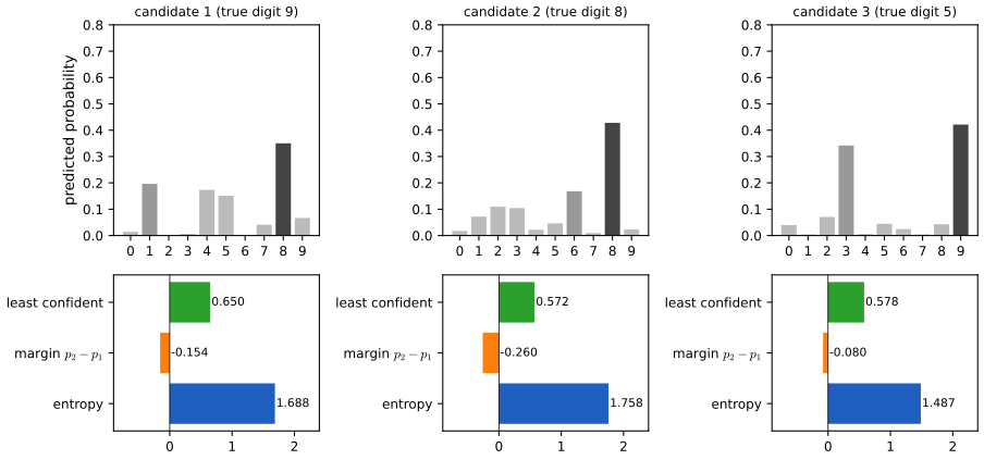
Filling the gap 34.27: how the three uncertainty scores relate, and what least confidence means pp. 1139–1141
Derivation
Two classes: all three agree. Let \(p_1\ge\tfrac12\) be the larger probability. Then entropy \(=-p_1\ln p_1-(1-p_1)\ln(1-p_1)\), margin score \(p_2-p_1=1-2p_1\), least-confident score \(=1-p_1\). All three are strictly decreasing functions of \(p_1\) on \([\tfrac12,1]\) (the derivative of the entropy is \(\ln\frac{1-p_1}{p_1}<0\)), so they order candidates identically. They can differ only for three or more classes. I verified the monotonicity on a grid.
Three or more classes: they can disagree. Least confidence uses only \(p_1\), the margin uses \(p_1,p_2\) and the entropy uses all probabilities. For \(p=(0.40,0.40,0.20)\) and \(q=(0.45,0.25,0.30)\): least confidence \(0.60\) against \(0.55\) and margin score \(0\) against \(-0.15\) both say \(p\) is more uncertain, but the entropies are \(1.055\) and \(1.067\) nats, so entropy prefers \(q\), whose probability is spread over three classes. Figure 34.17 shows the same on real predictions.
Least confidence is the Bayes risk. \(1-\max_cp_c\) is the posterior risk of the optimal action under 0-1 loss (34.15, 34.16). So least-confidence sampling queries the point with the largest current expected loss, which is not the same as the largest expected reduction of loss from the label (the value of information, gap 34.8, pml gap 19.15): an input whose label would not change the decision has zero value however uncertain it is. The information-theoretic scores of Section 34.7.3.3 address this.
34.7.3.2 Query by committee
pp. 1139–1141 For models that only return a prediction (an SVM), build a diverse ensemble of \(K\) members; disagreement among them plays the role of uncertainty (it can also be useful for probabilistic models, because model uncertainty can exceed parameter uncertainty; see deep ensembles, Section 17.3.9). With \(c^k_n\) the class predicted by member \(k\) for input \(x_n\) and \(v_{nc}=\sum_k\ind(c^k_n=c)\) the number of votes for class \(c\), the induced distribution is \[ q_{nc}=v_{nc}/K, \] the book prints \(v_{nc}/C\), which does not sum to one (the votes sum to \(K\), not to the number of classes \(C\)). Margin or entropy sampling is then applied to \(q_n\). This is query by committee (QBC; Seung, Opper and Sompolinsky 1992). For regression, the standard deviation of the members' predictions is used. In Figure 34.18 a committee of a random forest and a logistic regression is compared with margin sampling of the single forest and with random sampling.
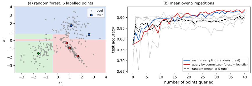
34.7.3.3 Information theoretic methods
p. 1141 Query the point whose label most reduces the uncertainty about the parameters \(w\) (Lindley 1956): the information gain \[ \alpha(x)=\Ent\big(p(w\given\D)\big)-\E_{p(y\given x,\D)}\Ent\big(p(w\given\D,x,y)\big)\tag{34.95} \] equals the expected change in the posterior, \(\alpha'(x)=\E_{p(y\given x,\D)}\KL\big(p(w\given\D,x,y)\,\|\,p(w\given\D)\big)\) (34.96), and by the symmetry of mutual information \[ \alpha(x)=\MI(w;y\given\D,x)=\Ent(y\given x,\D)-\E_{p(w\given\D)}\Ent(y\given x,w,\D). \tag{34.97–34.99} \] Bayesian active learning by disagreement (BALD; Houlsby et al. 2011) is (34.99): only entropies of the predictive distribution over \(y\) are needed. The first term alone is uncertainty sampling and is attracted to inherently ambiguous or mislabelled inputs; subtracting the expected entropy under fixed parameters removes that aleatoric part and keeps the epistemic part. Gap 34.28 proves the identities and gives a clean example.
Filling the gap 34.28: the BALD identities, the aleatoric/epistemic split, and BALD for Gaussian regression p. 1141, (34.95)–(34.99)
Derivation
Fix \(x\) and \(\D\); write \(p(w)\) for \(p(w\given\D)\), \(p(y\given w)\) for \(p(y\given x,w)\), \(p(y)=\sum_wp(w)p(y\given w)\) (sums become integrals for continuous variables).
All forms equal \(\MI(w;y)\). \(\MI(w;y)=\sum_{w,y}p(w,y)\ln\frac{p(w,y)}{p(w)p(y)}\). Writing \(p(w,y)=p(y)p(w\given y)\) gives \(\sum_yp(y)\sum_wp(w\given y)\ln\frac{p(w\given y)}{p(w)}=\E_y\KL(p(w\given y)\|p(w))\), which is (34.96). Splitting the logarithm gives \(\Ent(w)-\E_y\Ent(w\given y)\), i.e. (34.95) (the first term is constant in \(x\)). Writing instead \(p(w,y)=p(w)p(y\given w)\) gives \(\sum_{w}p(w)\sum_yp(y\given w)\ln\frac{p(y\given w)}{p(y)}=\Ent(y)-\E_w\Ent(y\given w)\), i.e. (34.99). A numerical experiment on a random finite model (4 parameter values, 3 labels) gives the same value, 0.1513, from all three expressions.
Aleatoric versus epistemic. \(\Ent(y)\) is the total predictive uncertainty. \(\E_w\Ent(y\given w)\) is what would remain if \(w\) were known (aleatoric, irreducible), so the difference is the part removable by learning \(w\) (epistemic). Example: let \(w\in\{w_1,w_2\}\) with probability \(\tfrac12\) each and two labels. Input A: \(p(y\given w_1)=p(y\given w_2)=(0.5,0.5)\): the predictive entropy is \(\ln2=0.693\) but \(\E_w\Ent(y\given w)=\ln2\), so BALD \(=0\): an ambiguous input where no label can teach anything. Input B: \(p(y\given w_1)=(0.9,0.1)\), \(p(y\given w_2)=(0.1,0.9)\): the predictive is \((0.5,0.5)\) with the same entropy \(0.693\), but \(\E_w\Ent=0.325\) and BALD \(=0.368\): the models disagree, and the label discriminates between them. Entropy sampling cannot tell A from B; BALD can.
Gaussian regression. If \(y=f(x)+\varepsilon\), \(\varepsilon\sim\N(0,\sigma_n^2)\) and the posterior of \(f(x)\) is \(\N(\mu,\sigma_f^2)\), then \(\MI(w;y)=\MI(f(x);y)=\Ent(y)-\Ent(y\given f)=\tfrac12\ln\big(2\pi e(\sigma_f^2+\sigma_n^2)\big)-\tfrac12\ln(2\pi e\sigma_n^2)=\tfrac12\ln\big(1+\sigma_f^2/\sigma_n^2\big)\), increasing in the predictive variance. So for a Gaussian process (or a linear-Gaussian model) BALD selects the input of largest predictive variance, which justifies the acquisition function of Figure 34.16a; pml gap 19.16 gives the same closed form and an approximation for BALD with logistic models. Because a GP's posterior variance does not depend on the observed \(y\), such a variance-driven design can be computed without waiting for labels.
34.7.4 Batch active learning
p. 1141 When retraining after every label is too slow, a batch of examples is labelled at once, and the batch must be diverse or it wastes labels on near-duplicates. BatchBALD (Kirsch, Van Amersfoort and Gal 2019) extends BALD to a batch.
34.7.4.1 BatchBALD
p. 1142–1143 Summing the individual BALD scores, \(\alpha_{\mathrm{BALD}}(x_{1:B})=\sum_{i=1}^B\MI(y_i;w\given x_i,\D)\) (34.100), double-counts information shared by similar points. BatchBALD uses the joint mutual information between the batch's labels and the parameters, \[ \alpha_{\mathrm{BBALD}}(x_{1:B})=\MI(y_{1:B};w\given x_{1:B},\D)=\Ent(y_{1:B}\given x_{1:B},\D)-\E_{p(w\given\D)}\Ent(y_{1:B}\given x_{1:B},w,\D), \tag{34.101} \] which, in the information diagram of Figure 34.19 (Yeung 1991; a diagram, not reproduced), is the area of the union \(\cup_iy_i\) intersected with \(w\) (34.102), and satisfies \(\alpha_{\mathrm{BBALD}}\le\alpha_{\mathrm{BALD}}\) with \[ \MI(y_{1:B};w\given x_{1:B},\D)=\sum_{i=1}^B\MI(y_i;w\given x_{1:B},\D)-\TC(y_{1:B}\given x_{1:B},\D), \tag{34.103} \] where \(\TC\) is the total correlation (Section 5.3.5.1). Gap 34.29 proves it.
34.7.4.2 Optimizing BatchBALD
p. 1142 Scoring all subsets is combinatorial, so the batch is built greedily: given the partial batch \(A_{n-1}\) add \(x_n=\argmax_{x\in\D_{\mathrm{pool}}\setminus A_{n-1}}\alpha_{\mathrm{BBALD}}(A_{n-1}\cup\{x\},p(w\given\D))\) (34.104). BatchBALD is monotone and submodular, so the greedy batch has at least \(1-1/e\approx0.63\) of the optimal score: the proof (for any information gain \(\MI(\theta;y_S)\) with labels conditionally independent given the parameters) is in pml gap 19.17, and a numerical experiment on random finite models (monotonicity, diminishing returns, and the greedy batch against the best of all subsets) is given in the code.
34.7.4.3 Computing BatchBALD
p. 1143 Dropping the conditioning, \(\alpha_{\mathrm{BBALD}}=\Ent(y_1,\dots,y_B)-\E_{p(w)}\Ent(y_1,\dots,y_B\given w)\) (34.105). The labels are conditionally independent given \(w\), so the second term is \(\sum_i\E_w\Ent(y_i\given w)\), estimated by averaging over posterior samples \(\hat w_s\), \(s=1,\dots,S\) (34.106). The joint entropy is estimated by enumerating all label sequences \(\hat y_{1:B}\) and using the Monte Carlo average of the joint predictive, \[ \Ent(y_{1:B})\approx-\sum_{\hat y_{1:B}}\Big(\frac1S\sum_s p(\hat y_{1:B}\given\hat w_s)\Big)\ln\Big(\frac1S\sum_sp(\hat y_{1:B}\given\hat w_s)\Big), \tag{34.107, 34.108} \] with a minus sign that the printed (34.108) omits. The joint probabilities of the partial batch are stored and extended by one point at each greedy step. Gap 34.29 discusses the bias of this estimate.
Filling the gap 34.29: the total-correlation identity, BALD against BatchBALD, and the Monte Carlo estimator pp. 1142–1143, (34.100)–(34.108)
Derivation
Assume \(y_1,\dots,y_B\) are conditionally independent given \(w\) (each is the label of its own input), and condition on \(x_{1:B},\D\) throughout.
(34.103). By conditional independence, \(\Ent(y_{1:B}\given w)=\sum_i\Ent(y_i\given w)\). Then \(\MI(y_{1:B};w)=\Ent(y_{1:B})-\sum_i\E_w\Ent(y_i\given w)\), whereas \(\sum_i\MI(y_i;w)=\sum_i\Ent(y_i)-\sum_i\E_w\Ent(y_i\given w)\). Subtracting, \(\sum_i\MI(y_i;w)-\MI(y_{1:B};w)=\sum_i\Ent(y_i)-\Ent(y_{1:B})=\TC(y_{1:B})\), the total correlation, which equals \(\KL\big(p(y_{1:B})\,\|\,\prod_ip(y_i)\big)\ge0\). This is (34.103), and \(\alpha_{\mathrm{BBALD}}\le\alpha_{\mathrm{BALD}}\) with equality iff the labels are independent in their predictive distribution, i.e. the batch members carry no overlapping information. For \(B=1\) the two coincide. (I verified (34.103) on a random finite model: \(\TC=0.0159\), and the monotonicity, diminishing returns and greedy bound on 60 random sets.) The BALD sum \(\sum_i\MI(y_i;w)\) as written in the book's (34.103) conditions the \(i\)th term on the whole batch of inputs; since each label depends only on its own input, this equals \(\MI(y_i;w\given x_i)\).
Monte Carlo estimator. Let \(\hat p(\hat y)=\frac1S\sum_sp(\hat y\given\hat w_s)\), an unbiased estimate of \(p(\hat y)\) for each \(\hat y\), consistent as \(S\to\infty\), so the plug-in entropy \(-\sum\hat p\ln\hat p\) is consistent. It is biased: the function \(\phi(u)=-u\ln u\) is concave, so by Jensen's inequality \(\E\phi(\hat p(\hat y))\le\phi(\E\hat p(\hat y))=\phi(p(\hat y))\) for each sequence, and the estimate is an underestimate of the joint entropy, with an error of order \(K^B/S\) for \(K\) classes (the number of sequences over the sample size). The estimate of the second term is unbiased. In a check with 5 candidates, 6 parameter values and 4000 samples the sampled BALD score (0.2208) agrees with the exact value (0.2213) and the greedy batch is the exact greedy batch.
Slips in the printed equations. (34.106) sums over \(i=1,\dots,n\) where it should run to \(B\); (34.107) has a typo ("\(\mathrm vw\)" for \(w\)); (34.108) lacks the minus sign of the entropy; and the sum over \(\hat y_{1:B}\) has \(K^B\) terms (\(10^4\) for MNIST with \(B=4\)), which is why the incremental update is needed.
34.7.4.4 Experimental comparison of BALD vs BatchBALD on MNIST
p. 1144 The book trains a CNN on MNIST with batch size 4, approximating \(p(w\given\D)\) by MC dropout (Section 17.3.1): BALD picks near-duplicate examples and BatchBALD picks diverse ones (Figure 34.20a, b), and BatchBALD learns more efficiently, which in turn beats random sampling (Figure 34.20c). My reproduction is scaled down to what a laptop CPU does in a few minutes: the 8 by 8 scikit-learn digits (500 for test and a pool of 500 candidates drawn from the remaining 1,297), a one-hidden-layer dropout network (64 units, dropout 0.25) retrained from scratch at each round, \(S=24\) dropout samples, batch size 4, 20 rounds from 20 initial labels (2 per class), BatchBALD with exact enumeration of up to \(10^4\) label sequences, on the 150 pool points of highest BALD score, and 3 repetitions.
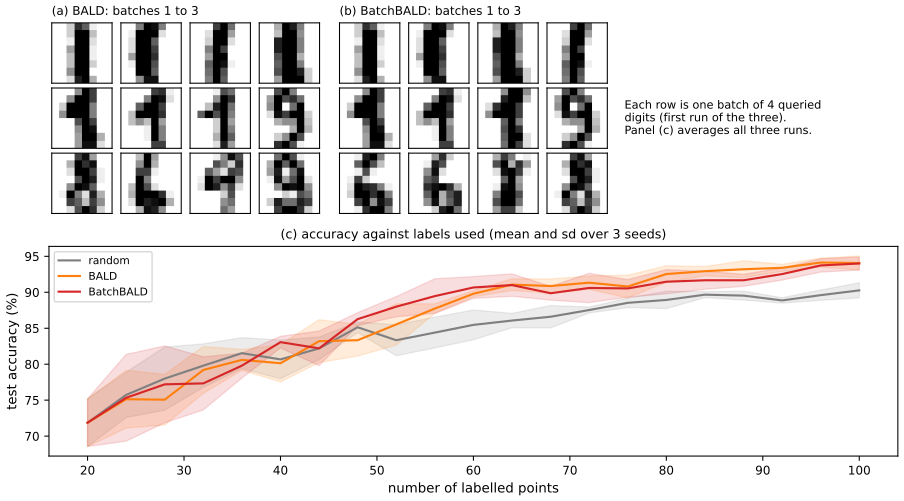
The comparison to random sampling is clear (about 4 to 5 percentage points at 60 and 100 labels); the difference between BALD and BatchBALD is not resolved here. The BatchBALD paper reports a larger advantage for larger batches, where the double counting of near-duplicates is worse; with \(B=4\) and a small network, the overlap that BatchBALD removes is modest.
Supplement S34
The supplement chapter S34, titled "Multi-step decision problems" (pages 307 and 308 of the supplement), consists of a title page and a blank page in this draft; there is no content to cover. The multi-step material of this chapter (MDPs, planning, bandits) is in Sections 34.4 to 34.6 of the main text.
Demonstrations
Practice problems
The book has no exercises for this chapter. These three short problems are my own.
Practice problem 34.1 (sizing an A/B test). A population of \(N=20{,}000\) users, prior \(\mu_j\sim\N(0.5,0.1^2)\) for the mean reward of each arm, noise standard deviation \(\sigma=0.5\). Find the optimal test size per arm, the expected total reward, the probability of deploying the worse arm, and check the bound in (34.43).
Solution
\(u^2=\sigma^2/\tau^2=25\), so \(n^*=\sqrt{\tfrac N4u^2+(\tfrac34u^2)^2}-\tfrac34u^2=\sqrt{125000+351.6}-18.75=354.05-18.75=335.3\); the bound is \(\sqrt N\sigma/(2\tau)=353.6\), satisfied. At \(n=335\): \(s=\sqrt{\tau^2+\sigma^2/n}=\sqrt{0.01+0.000746}=0.10366\), so the gain term is \((N-2n)\tau^2/(\sqrt\pi s)=19330\cdot0.05443=1052.0\) and \(\E[R]=Nm+1052.0=11052.0\) (the oracle earns \(N(m+\tau/\sqrt\pi)=11128.4\), so the regret is about 76). The error rate is \(\tfrac12-\tfrac1\pi\arctan(\tau\sqrt n/\sigma)=\tfrac12-\tfrac1\pi\arctan(3.66)=0.0848\), i.e. 8.5% (not the 4.2% that the printed (34.47) would give). My code confirms these numbers (
ab_nstar,ab_expected_reward,ab_error_rate) and a simulation of the whole procedure agrees (gap 34.11, 34.12, 34.14).Practice problem 34.2 (policy iteration by hand). An MDP has two states and two actions (stay, move), deterministic: moving swaps the states. Rewards: \(R(1,\text{stay})=0\), \(R(1,\text{move})=1\), \(R(2,\text{stay})=2\), \(R(2,\text{move})=0\); \(\gamma=\tfrac12\). Run policy iteration from \(\pi_0=(\text{stay},\text{move})\), and say how many value-iteration sweeps from \(V_0=0\) are needed to get within \(0.01\) of \(V_*\).
Solution
Evaluate \(\pi_0\): state 1 stays with reward 0, so \(V(1)=0\); state 2 moves to 1 with reward 0, so \(V(2)=\tfrac12V(1)=0\); \(V_{\pi_0}=(0,0)\). Improve: \(Q(1,\text{move})=1+0=1>Q(1,\text{stay})=0\), \(Q(2,\text{stay})=2>Q(2,\text{move})=0\): \(\pi_1=(\text{move},\text{stay})\). Evaluate: \(V(2)=2+\tfrac12V(2)\Rightarrow V(2)=4\); \(V(1)=1+\tfrac12V(2)=3\). Improve: \(Q(1,\text{stay})=\tfrac12\cdot3=1.5<3\) and \(Q(2,\text{move})=\tfrac12\cdot3=1.5<4\): \(\pi_1\) is greedy for its own value, so it is optimal, with \(V_*=(3,4)\), after 2 improvement steps. Value iteration from \(V_0=0\) gives \(V_1=(1,2)\), \(V_2=(2,3)\), \(V_3=(2.5,3.5)\), \(V_4=(2.75,3.75),\dots\), so \(\|V_k-V_*\|_\infty=2^{2-k}=\gamma^k\|V_0-V_*\|_\infty\) for \(k\ge1\): the contraction bound (34.87) is attained here. The error is at most \(0.01\) once \(2^{2-k}\le0.01\), i.e. \(k=9\) (error \(0.0078\)), against 2 policy-iteration steps. My code reproduces \(V_*=(3,4)\) and the policy.
Practice problem 34.3 (the Lai-Robbins constant). Two Bernoulli arms with means \(0.6\) and \(0.5\). Compute the constant in the lower bound (34.73) and compare with the Gaussian value \(2\sigma^2/\Delta\) for the variance \(\sigma^2=\tfrac14\) of a fair Bernoulli.
Solution
\(\Delta=0.1\) and \(\KL(\mathrm{Ber}(0.5)\|\mathrm{Ber}(0.6))=0.5\ln\tfrac{0.5}{0.6}+0.5\ln\tfrac{0.5}{0.4}=0.5(-0.18232+0.22314)=0.020411\). The constant is \(\Delta/\KL=0.1/0.020411=4.899\) per unit of \(\ln T\): any consistent policy has regret of at least about \(4.9\ln T\) asymptotically, e.g. 45 at \(T=10^4\). The Gaussian formula with \(\sigma^2=\tfrac14\) gives \(\Delta/(\Delta^2/2\sigma^2)=2\sigma^2/\Delta=5.0\); the two agree to 2% because \(\KL(\mathrm{Ber}(p)\|\mathrm{Ber}(q))\approx(p-q)^2/(2q(1-q))\) for close means, with \(q(1-q)\approx0.25\). With a unit-variance Gaussian the constant would be \(2/0.1=20\): noisier rewards are harder to learn from. See gap 34.19.
Notes on the book
Slips and sharpenings found while proving and checking the claims
- Section 34.2.2, (34.29). The maximum expected utility with the sounding is \(0.35\cdot32.857+0.24\cdot87.5=32.5\), not 32.2, and the value of the sounding is 12.5, not 12.2 (the rounded numbers in the text already give \(11.52+21=32.5\)). Gap 34.7.
- Section 34.2.3. The quantity (34.30) is the expected value of sample information for the noisy sounding (12.5); the value of perfect information (observing the oil state) is \(55-20=35\). Gap 34.8.
- Section 34.3.1.4, (34.46) and (34.47). For \(\mu_1<\mu_0\) the probability of picking arm 1 is \(\Phi((\mu_1-\mu_0)/(\sigma\sqrt{1/n_1+1/n_0}))\); the printed \(1-\Phi\) of that argument has the wrong sign. Equation (34.47) is the joint probability \(\Pr(\pi=1,\mu_1<\mu_0)\); the probability of deploying the wrong arm, which is the book's "10%", is twice it, \(\tfrac12-\tfrac1\pi\arctan(\cdot)\). Gap 34.14.
- Section 34.3.2. Under the stated prior the expected effect size is \(\E|\mu_1-\mu_0|=2\tau/\sqrt\pi=0.034\), not 0.023 (that is \(\E|\mu_j-m|\)).
- Section 34.1.5.5, (34.23), (34.24). "min" should be "argmin" in (34.23); the sample estimate should be the unweighted average \(\frac1M\sum_j\ell(y_j,y_i)\): weighting samples from \(p\) again by \(p(y_j\given x)\) estimates the wrong quantity. Gap 34.5.
- Section 34.4.4, (34.57). With \(N^r_t(a)\) counting rewards equal to \(r\), the Beta parameters should be \(\alpha_0^a+N^1_t(a)\) and \(\beta_0^a+N^0_t(a)\) (successes increase \(\alpha\)); the printed assignment is swapped.
- Section 34.4.5.2, (34.65). The plug-in standard deviation is zero for an arm with only failures (or only successes), which can lock the arm out; use the Beta posterior's own standard deviation. Gap 34.17.
- Section 34.4.7, (34.73). The statement is a bound on \(\liminf_TL_T/\ln T\); it is not a bound on the regret at every finite \(T\), and fixed-\(\varepsilon\) greedy (not consistent) can have smaller regret than \(C\ln T\) at moderate \(T\). Gap 34.19.
- Section 34.5.5.1. At \(\gamma=1\), \(Q_*\) is 1 for all state-action pairs except \((s_1,\text{up})\), which is 0 (the figure shows this; the sentence says "all"). Gap 34.22.
- Section 34.6.2, (34.90). The last expression should read \((I-\gamma T')^{-1}r'=v'\), with \(r'\) in place of \(r\). Gap 34.25.
- Section 34.6.3, (34.92). The constraint should contain \(V(s')\) inside the sum over next states, not \(V(s)\). Gap 34.26.
- Section 34.7.3.2. The vote distribution is \(q_{nc}=v_{nc}/K\) (number of committee members), not \(v_{nc}/C\). 34.7.3.2.
- Section 34.7.4.3. (34.106) should sum over \(i=1,\dots,B\); (34.107) contains a typo (\(\mathrm vw\)); (34.108) lacks the minus sign of the entropy. Gap 34.29.
References
- Murphy, K. P. (2023). Probabilistic Machine Learning: Advanced Topics. MIT Press, Cambridge, MA. Chapter 34, pp. 1105–1144. probml.github.io/pml-book/book2.html.
- Agrawal, S. and Goyal, N. (2012). Analysis of Thompson sampling for the multi-armed bandit problem. Conference on Learning Theory.
- Audibert, J.-Y., Bubeck, S. and Munos, R. (2010). Best arm identification in multi-armed bandits. Conference on Learning Theory.
- Auer, P., Cesa-Bianchi, N. and Fischer, P. (2002). Finite-time analysis of the multiarmed bandit problem. Machine Learning, 47, 235–256.
- Barto, A. G., Bradtke, S. J. and Singh, S. P. (1995). Learning to act using real-time dynamic programming. Artificial Intelligence, 72, 81–138.
- Berger, J. O. (1985). Statistical Decision Theory and Bayesian Analysis, 2nd edition. Springer.
- DeGroot, M. H. (1970). Optimal Statistical Decisions. McGraw-Hill.
- Feit, E. M. and Berman, R. (2019). Test and roll: profit-maximizing A/B tests. Marketing Science, 38(6), 1038–1058.
- Ferguson, T. S. (1967). Mathematical Statistics: A Decision Theoretic Approach. Academic Press.
- Gittins, J. C. (1989). Multi-armed Bandit Allocation Indices. Wiley.
- Houlsby, N., Huszár, F., Ghahramani, Z. and Lengyel, M. (2011). Bayesian active learning for classification and preference learning. arXiv:1112.5745.
- Kaufmann, E., Korda, N. and Munos, R. (2012). Thompson sampling: an asymptotically optimal finite-time analysis. Algorithmic Learning Theory.
- Kirsch, A., van Amersfoort, J. and Gal, Y. (2019). BatchBALD: efficient and diverse batch acquisition for deep Bayesian active learning. Advances in Neural Information Processing Systems, 32.
- Kjaerulff, U. B. and Madsen, A. L. (2008). Bayesian Networks and Influence Diagrams. Springer.
- Kochenderfer, M. J., Wheeler, T. A. and Wray, K. H. (2022). Algorithms for Decision Making. MIT Press.
- Lai, T. L. and Robbins, H. (1985). Asymptotically efficient adaptive allocation rules. Advances in Applied Mathematics, 6, 4–22.
- Lattimore, T. and Szepesvári, C. (2020). Bandit Algorithms. Cambridge University Press.
- Lauritzen, S. L. and Nilsson, D. (2001). Representing and solving decision problems with limited information. Management Science, 47(9), 1235–1251.
- Lindley, D. V. (1956). On a measure of the information provided by an experiment. Annals of Mathematical Statistics, 27(4), 986–1005.
- Nemhauser, G. L., Wolsey, L. A. and Fisher, M. L. (1978). An analysis of approximations for maximizing submodular set functions I. Mathematical Programming, 14, 265–294.
- Puterman, M. L. (1994). Markov Decision Processes: Discrete Stochastic Dynamic Programming. Wiley.
- Russo, D. and Van Roy, B. (2014). Learning to optimize via posterior sampling. Mathematics of Operations Research, 39(4), 1221–1243.
- Sutton, R. S. and Barto, A. G. (2018). Reinforcement Learning: An Introduction, 2nd edition. MIT Press.
- Thompson, W. R. (1933). On the likelihood that one unknown probability exceeds another in view of the evidence of two samples. Biometrika, 25, 285–294.
- Wald, A. (1947). An essentially complete class of admissible decision functions. Annals of Mathematical Statistics, 18(4), 549–555.
The numerical statements in the text (the wildcatter's posteriors, maximum expected utility and values of information, the cube example and the max-marginal estimate, the binomial minimax risk, the optimal A/B test size, its reward, regret and error rate against simulation, the Beta-Bernoulli and normal-inverse-gamma updates, probability matching, the exact Bayes-optimal bandit values, the UCB1 bound, the Lai-Robbins constant, the grid-world Q-functions, the contraction and stopping bounds of value iteration, the monotonicity of policy iteration, the agreement of value iteration, policy iteration and both linear programs, the identities for BALD and BatchBALD, and the practice problems) were confirmed numerically.