Probability: Multivariate Models
Chapter 2 dealt with one random variable at a time. Machine learning almost always deals with many, and the interesting questions are about how they depend on one another: how strongly, in which direction, through which hidden cause. This chapter builds the tools for that. Covariance and correlation measure linear dependence, and the chapter is careful about what they do not measure. The multivariate Gaussian is the one joint distribution for which everything (marginals, conditionals, noisy observation, fusion of several measurements) can be written in closed form, so it is studied in detail. The exponential family explains why so many standard distributions share these closed forms, mixture models build richer densities out of simple ones, and directed graphical models show how a large joint distribution is assembled from small conditional pieces.
Ch. 1 Introduction Ch. 2 Univariate probability Ch. 3 Multivariate probability Ch. 4 Statistics Ch. 5 Decision theory Ch. 6 Information theory Ch. 7 Linear algebra Ch. 8 Optimisation Ch. 9 Discriminant analysis Ch. 10 Logistic regression Ch. 11 Linear regression Ch. 12 GLMs Ch. 13 Networks for tabular data Ch. 14 Networks for images Ch. 15 Networks for sequences Ch. 16 Exemplar-based methods Ch. 17 Kernel methods Ch. 18 Trees and boosting Ch. 19 Fewer labels Ch. 20 Dimensionality reduction Ch. 21 Clustering Ch. 22 Recommender systems Ch. 23 Graph embeddings
How to read these notes
They follow the book. Sections carry the book's numbers (3.1, 3.2.3, ...) and every displayed equation that appears in the book carries the book's own number, e.g. \((3.28)\), so you can read these notes next to the book. Equations without a number are steps that the book skips.
Filling the gaps. Wherever the book says "one can show", leaves a result to an exercise, or quotes a formula without proof, an orange Filling the gap box or a proof gives the full argument. Proofs and derivations start hidden: open one with its bar, or use the button below.
Figures and demonstrations. Every figure of the chapter that is computed from data, a model or a simulation is reproduced from scratch by the Python code; the four network diagrams (Figures 3.14 to 3.17) are not redrawn, but the probabilities in Figure 3.14 are computed. The ▶ Demo boxes open an interactive demonstration already set to the case being discussed.
Main reference
K. P. Murphy, Probabilistic Machine Learning: An Introduction, MIT Press (2022; the April 2025 online draft is the version read here), Chapter 3, pages 77–105 (book web page: probml.github.io/pml-book/book1.html). Section, equation, figure and exercise numbers below refer to this book. Further reading is listed in the references.
The explanations, derivations, figures and code are my own; equations are cited by their numbers in the book.
Companion courses
Much of this chapter also appears, with proofs, in two other courses on this site. Read those for the full story and come back here for Murphy's notation and examples.
- Bayesian and Probabilistic Machine Learning (Bishop, 2006): Gaussian conditionals, marginals and Bayes' theorem for Gaussians, Sections 2.3.1–2.3.3; Bayesian inference for the Gaussian, Section 2.3.6; mixtures of Gaussians, Section 2.3.9 and Chapter 9; the exponential family, Section 2.4; directed graphical models, Section 8.1.
- Probability and Statistical Inference (Wasserman, 2004): covariance and correlation, Section 3.3; random vectors and the multivariate normal, Section 14.3; independence and association, Chapter 15; directed graphs, Chapter 17.
Companion demonstrations on the same ideas: conjugate priors, mixture densities, K-means and EM, d-separation.
The chapter at a glance
- 3.1.1–3.1.3 Covariance is bilinear and transforms as \(\mathbf{A}\boldsymbol\Sigma\mathbf{A}^\T\) (Filling the gap 3.1); \(|\rho|\le1\) with equality exactly for a linear relation (Result 3.1); the regression slope is \(\rho\sigma_Y/\sigma_X\) (gap 3.2); independence implies zero correlation but not conversely (Result 3.2), except for jointly Gaussian variables (gap 3.3).
- 3.1.4–3.1.5 A hidden common cause makes unrelated series correlated (gap 3.4); a trend can reverse in a mixture of groups because an overall rate is a weighted average (Result 3.3).
- 3.2 The Gaussian density normalises to one and has mean and covariance \(\boldsymbol\mu,\boldsymbol\Sigma\) (gap 3.5); its level sets are ellipses with axes along the eigenvectors (Result 3.4); marginals and conditionals are Gaussian with the Schur complement as conditional covariance (Result 3.5); conditioning is optimal imputation (gap 3.8).
- 3.3 Bayes rule for Gaussians adds precisions (Result 3.6); for a scalar the posterior mean is a convex combination of prior mean and data (gap 3.10); \(N\) observations are equivalent to their average (gap 3.11); sensors are weighted by precision (gap 3.12).
- 3.4 The log partition function is convex and its derivatives are the cumulants of the sufficient statistics (Result 3.7); maximum entropy under moment constraints gives an exponential family (Result 3.8); the book's definition of minimality needs a correction (note).
- 3.5 Mixture moments, responsibilities and the K-means limit (gap 3.13); EM updates for a Bernoulli mixture (gap 3.14).
- 3.6 The ordered Markov property is equivalent to the factorisation along the graph (Result 3.9), which also counts the parameters; explaining away computed by hand (gap 3.15); iid data are exchangeable (gap 3.16).
Notation. Random vectors are bold lower case (\(\mathbf{x},\mathbf{y},\mathbf{z}\)), \(\mathbb V\) is variance, \(\operatorname{Cov}\) covariance. A covariance matrix is \(\boldsymbol\Sigma\); a precision matrix is \(\boldsymbol\Lambda=\boldsymbol\Sigma^{-1}\). \(\mathcal N(\mathbf y\given\boldsymbol\mu,\boldsymbol\Sigma)\) is the Gaussian density. Densities of positive definite \(\boldsymbol\Sigma\) are assumed throughout, except where a limit is stated.
Prerequisites. Chapter 2 of the book (random variables, expectation, the univariate Gaussian) and basic linear algebra: eigendecomposition of symmetric matrices, block matrices. The toolkit of the companion course has what is needed.
3.1 Joint distributions for multiple random variables
p. 77 This section is about measuring how random variables depend on each other, and about the many ways such a measurement can mislead.
See also (companion course): Probability and Statistical Inference, Section 3.3 (variance and covariance, with proofs).
3.1.1 Covariance
Definition 3.1 (covariance and covariance matrix) p. 77, (3.1)–(3.6)
For random variables \(X,Y\) with finite second moments,
\[ \cov[X,Y]=\E\big[(X-\E X)(Y-\E Y)\big]=\E[XY]-\E[X]\,\E[Y]. \tag{3.1} \]For a random vector \(\mathbf{x}\in\R^D\) the covariance matrix has entries \(\Sigma_{ij}=\cov[X_i,X_j]\) (so the diagonal holds the variances \(\mathbb V[X_i]\)):
\[ \cov[\mathbf{x}]=\E\big[(\mathbf{x}-\E\mathbf{x})(\mathbf{x}-\E\mathbf{x})^\T\big]=\boldsymbol\Sigma. \tag{3.2} \]The cross-covariance of two random vectors is \(\cov[\mathbf{x},\mathbf{y}]=\E[(\mathbf{x}-\E\mathbf{x})(\mathbf{y}-\E\mathbf{y})^\T]\) (3.6).
Filling the gap 3.1: \(\boldsymbol\Sigma\) is positive semidefinite, \(\E[\mathbf{x}\mathbf{x}^\T]=\boldsymbol\Sigma+\boldsymbol\mu\boldsymbol\mu^\T\), and \(\cov[\mathbf{A}\mathbf{x}+\mathbf{b}]=\mathbf{A}\boldsymbol\Sigma\mathbf{A}^\T\) p. 77, (3.2)–(3.5)
The book calls \(\boldsymbol\Sigma\) "symmetric, positive semidefinite" and states (3.4) and (3.5) with a pointer to Exercise 3.4. Here are all of them.
Derivation
(3.4). Write \(\mathbf{x}=\boldsymbol\mu+(\mathbf{x}-\boldsymbol\mu)\) with \(\boldsymbol\mu=\E\mathbf{x}\) and expand: \[\mathbf{x}\mathbf{x}^\T=\boldsymbol\mu\boldsymbol\mu^\T+\boldsymbol\mu(\mathbf{x}-\boldsymbol\mu)^\T+(\mathbf{x}-\boldsymbol\mu)\boldsymbol\mu^\T+(\mathbf{x}-\boldsymbol\mu)(\mathbf{x}-\boldsymbol\mu)^\T\]. Taking expectations, the two cross terms vanish because \(\E(\mathbf{x}-\boldsymbol\mu)=\mathbf{0}\), leaving \(\E[\mathbf{x}\mathbf{x}^\T]=\boldsymbol\mu\boldsymbol\mu^\T+\boldsymbol\Sigma\).
(3.5). \(\E[\mathbf{A}\mathbf{x}+\mathbf{b}]=\mathbf{A}\boldsymbol\mu+\mathbf{b}\), so \(\mathbf{A}\mathbf{x}+\mathbf{b}-\E[\cdot]=\mathbf{A}(\mathbf{x}-\boldsymbol\mu)\), and \[\cov[\mathbf{A}\mathbf{x}+\mathbf{b}]=\E[\mathbf{A}(\mathbf{x}-\boldsymbol\mu)(\mathbf{x}-\boldsymbol\mu)^\T\mathbf{A}^\T]=\mathbf{A}\boldsymbol\Sigma\mathbf{A}^\T\], since expectation is linear and \(\mathbf{A}\) is constant.
Symmetric and positive semidefinite. \(\Sigma_{ij}=\Sigma_{ji}\) is clear from (3.1). For any fixed vector \(\mathbf{v}\), \((3.5)\) with \(\mathbf{A}=\mathbf{v}^\T\) gives \(\mathbf{v}^\T\boldsymbol\Sigma\mathbf{v}=\cov[\mathbf{v}^\T\mathbf{x}]=\mathbb V[\mathbf{v}^\T\mathbf{x}]\ge0\). Moreover \(\mathbf{v}^\T\boldsymbol\Sigma\mathbf{v}=0\) exactly when \(\mathbf{v}^\T\mathbf{x}\) is almost surely constant, so \(\boldsymbol\Sigma\) is positive definite unless the components of \(\mathbf{x}\) satisfy an exact affine relation. ∎
3.1.2 Correlation
Definition 3.2 (correlation) pp. 78–79, (3.7)–(3.10)
For \(\mathbb V[X],\mathbb V[Y]>0\), the (Pearson) correlation coefficient is
\[ \rho=\corr[X,Y]=\frac{\cov[X,Y]}{\sqrt{\mathbb V[X]\,\mathbb V[Y]}}. \tag{3.7} \]For a vector, \(\corr(\mathbf{x})=\diag(\boldsymbol\Sigma)^{-1/2}\,\boldsymbol\Sigma\,\diag(\boldsymbol\Sigma)^{-1/2}\) (3.9): entry \((i,j)\) is \(\Sigma_{ij}/\sqrt{\Sigma_{ii}\Sigma_{jj}}\), and the diagonal is 1.
Result 3.1 (\(|\rho|\le1\), with equality exactly for linear relations; Exercises 3.2 and 3.3) p. 78
(a) \(-1\le\rho\le1\). (b) \(\rho=1\) if and only if \(Y=aX+b\) almost surely for some \(a>0\) and \(b\); \(\rho=-1\) if and only if this holds with \(a\lt 0\).
Proof
Put \(U=(X-\E X)/\sigma_X\) and \(V=(Y-\E Y)/\sigma_Y\); then \(\E U=\E V=0\), \(\E U^2=\E V^2=1\) and \(\E[UV]=\rho\). Expand \[\E[(U\mp V)^2]=1+1\mp2\rho=2(1\mp\rho)\ge0\], so \(-1\le\rho\le1\), proving (a).
For (b): \(\rho=1\) iff \(\E[(U-V)^2]=0\) iff \(U=V\) almost surely (a nonnegative variable with zero mean is zero a.s.), i.e. \(Y=\E Y+\tfrac{\sigma_Y}{\sigma_X}(X-\E X)\), which is \(aX+b\) with \(a=\sigma_Y/\sigma_X>0\). Conversely if \(Y=aX+b\) with \(a>0\) then \(\cov[X,Y]=a\mathbb V[X]\) and \(\mathbb V[Y]=a^2\mathbb V[X]\), so \(\rho=a\mathbb V[X]/(|a|\mathbb V[X])=\operatorname{sgn}(a)\). The case \(\rho=-1\) is the same with \(U=-V\). ∎
Filling the gap 3.2: correlation is not the slope p. 78
The book says that the regression coefficient is \(a=\cov[X,Y]/\mathbb V[X]\) and points to Equation (11.27). Here is the short argument and what it implies.
Derivation
Among all lines \(aX+b\), the one minimising the mean squared error \(\E[(Y-aX-b)^2]\) satisfies the two first-order conditions \(\E[Y-aX-b]=0\) and \(\E[X(Y-aX-b)]=0\). The first gives \(b=\E Y-a\E X\); substituting in the second gives \(\cov[X,Y]-a\mathbb V[X]=0\), so \(a=\cov[X,Y]/\mathbb V[X]\). The objective is a convex quadratic in \((a,b)\), so this is the minimum. Since \(\cov[X,Y]=\rho\sigma_X\sigma_Y\),
\[ a=\rho\,\frac{\sigma_Y}{\sigma_X}. \]Hence the slope changes with the units of \(X\) and \(Y\) while \(\rho\) does not (replace \(X\) by \(cX\), \(c>0\): \(a\) becomes \(a/c\), \(\rho\) is unchanged). In the middle row of Figure 3.1, lines of very different slopes all have \(\rho=1\). The minimum error is \(\E[(Y-aX-b)^2]=\sigma_Y^2(1-\rho^2)\), so \(\rho^2\) is the fraction of the variance of \(Y\) explained by the best linear predictor: the "degree of linearity" of the book. ∎
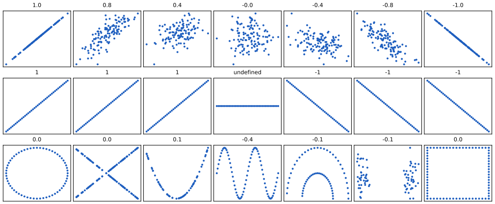
fig_3_1. Download: PDF · SVGSee also (companion course): Probability and Statistical Inference, Section 14.2 (estimating the correlation).
3.1.3 Uncorrelated does not imply independent
Result 3.2 (independent \(\Rightarrow\) uncorrelated, not conversely; Exercise 3.1) p. 79
If \(X\) and \(Y\) are independent with finite second moments then \(\cov[X,Y]=0\). The converse fails: for \(X\sim U(-1,1)\) and \(Y=X^2\), \(\corr[X,Y]=0\) although \(Y\) is a function of \(X\).
Proof
If \(X\) and \(Y\) are independent, \(\E[XY]=\E[X]\E[Y]\) (the joint density factorises, so the double integral does), which is \(\cov[X,Y]=0\) by (3.1). For the counterexample, \(\E X=0\), \(\E[XY]=\E[X^3]=\int_{-1}^{1}x^3\tfrac12\d x=0\) (odd integrand), so \(\cov[X,Y]=\E[X^3]-\E X\,\E X^2=0\). Also \[\mathbb V[Y]=\E X^4-(\E X^2)^2=\tfrac15-\tfrac19=\tfrac4{45}>0\], so the correlation is defined and equals 0. ∎
The information-theoretic measure that does detect any dependence, the mutual information, is zero exactly for independent variables (Section 6.3 of the book).
Filling the gap 3.3: jointly Gaussian and uncorrelated does imply independent; marginally Gaussian does not suffice p. 79; Exercise 3.5
Derivation
Positive result. Let \((Y_1,Y_2)\) be jointly Gaussian with \(\cov[Y_1,Y_2]=0\). Then \(\boldsymbol\Sigma=\diag(\sigma_1^2,\sigma_2^2)\), \(|\boldsymbol\Sigma|=\sigma_1^2\sigma_2^2\), and the quadratic form in (3.11) splits as \((y_1-\mu_1)^2/\sigma_1^2+(y_2-\mu_2)^2/\sigma_2^2\), so the joint density is the product \(\mathcal N(y_1\given\mu_1,\sigma_1^2)\mathcal N(y_2\given\mu_2,\sigma_2^2)\): independent.
The hypothesis "jointly" cannot be dropped (Exercise 3.5). Let \(X\sim\mathcal N(0,1)\), \(W\) independent of \(X\) with \(\Pr(W=\pm1)=\tfrac12\), and \(Y=WX\). (a) For any \(y\), \[\Pr(Y\le y)=\tfrac12\Pr(X\le y)+\tfrac12\Pr(-X\le y)=\Phi(y)\] because \(-X\sim\mathcal N(0,1)\), so \(Y\sim\mathcal N(0,1)\). (b) By iterated expectation, \[\E[XY]=\E[\E[WX^2\given W]]=\E[W]\,\E[X^2]=0\], and \(\E X=\E Y=0\), so \(\cov[X,Y]=0\). Yet \(Y^2=X^2\), so \(\cov[X^2,Y^2]=\mathbb V[X^2]=2\ne0\): \(X\) and \(Y\) are dependent. The pair is not jointly Gaussian: \(X+Y=(1+W)X\) equals 0 with probability \(\tfrac12\), whereas every linear combination of a Gaussian vector is either Gaussian (hence has no point mass) or an exactly constant. ∎
3.1.4 Correlation does not imply causation
pp. 79–80 Two series can move together because both respond to a third, unmeasured, variable. Figure 3.2 shows the standard example (ice cream sales and violent crime, both driven by the weather) with simulated data.
Filling the gap 3.4: how much correlation can a hidden common cause create? p. 79
Derivation
Let the temperature \(T\) have variance \(\sigma_T^2\) and set \(X=\alpha T+\varepsilon_1\), \(Y=\beta T+\varepsilon_2\) with \(\varepsilon_1,\varepsilon_2,T\) independent and of mean zero (an intercept changes nothing). Then \(\cov[X,Y]=\alpha\beta\sigma_T^2\) by bilinearity, since all other cross terms vanish, and
\[ \corr[X,Y]=\frac{\alpha\beta\sigma_T^2}{\sqrt{(\alpha^2\sigma_T^2+\sigma_1^2)(\beta^2\sigma_T^2+\sigma_2^2)}}, \]which tends to \(\pm1\) as the noises \(\sigma_1^2,\sigma_2^2\to0\), although \(X\) has no effect on \(Y\). Removing the part of each variable explained by \(T\) (regressing both on \(T\) and correlating the residuals, the partial correlation) leaves \(\varepsilon_1,\varepsilon_2\), which are uncorrelated. Figure 3.2(c) shows this for the simulation. The lesson is only that a predictive association is not evidence of an effect; deciding causal questions needs either an experiment or explicit causal assumptions (see the companion course on causal inference). ∎
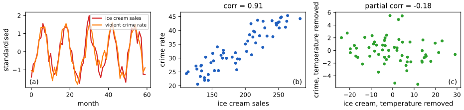
fig_3_2. Download: PDF · SVG3.1.5 Simpson's paradox
pp. 80–81 A relationship that holds in every subgroup can disappear or reverse when the groups are combined. Figure 3.3 shows it on the iris data: within each species sepal width increases with sepal length, but across all 150 flowers it decreases.
Result 3.3 (Simpson's reversal is a statement about weighted averages) p. 80, Figures 3.3–3.4
Let a population be divided into groups \(a=1,\dots,A\) (for instance age bands) and let a binary outcome \(F\) (death) have group rate \(r_a^{C}=\Pr(F=1\given a,C)\) in country \(C\) and group share \(w_a^{C}=\Pr(a\given C)\). Then
\[ \Pr(F=1\given C)=\sum_{a=1}^{A}r_a^{C}\,w_a^{C}. \]It is possible that \(r_a^{B}\le r_a^{A}\) for every group \(a\) and yet \(\Pr(F=1\given B)>\Pr(F=1\given A)\), if \(B\)'s shares \(w^B\) put much more weight than \(w^A\) on the groups with high rates.
Proof, and a numerical example
The identity is the law of total probability. The reversal needs no more than the observation that two weighted averages can compare in the opposite order to the termwise comparison of their values when their weights differ. Concretely, take two groups with \(r^A=(0.1,\,10)\%\), \(r^B=(0.1,\,8)\%\) (B is lower in both) and shares \(w^A=(0.9,0.1)\), \(w^B=(0.1,0.9)\): the totals are \(0.09+1.0=1.09\%\) for A and \(0.01+7.2=7.21\%\) for B. The figure uses nine age bands: B's rates are exactly 80% of A's in every band, but B's cases are concentrated at older ages (the shares and rates are printed in the code), and the overall rate is 2.88% for A and 6.05% for B. The interpretation is causal only if one is careful: here age is a confounder of the comparison of countries, and the fair comparison is within age band (or a weighted average with a common standard weighting), not the crude total. In the iris example the "weights" are the species, whose members differ in location so strongly that the pooled cloud tilts the other way (the three within-species correlations are \(0.74,0.53,0.46\); pooled, \(-0.12\)). ∎
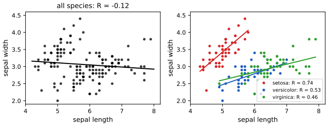
fig_3_3. Download: PDF · SVG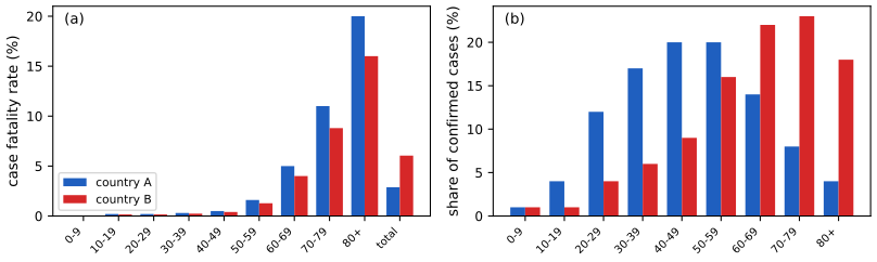
fig_3_4. Download: PDF · SVG3.2 The multivariate Gaussian (normal) distribution
p. 80 The multivariate normal (MVN) is the most widely used joint distribution for continuous variables, partly because it is mathematically convenient (this section and the next), partly because sums of many small effects are approximately Gaussian (Section 2.6.4 of the book).
See also (companion courses): Bayesian and Probabilistic Machine Learning, Section 2.3 (the Gaussian distribution) and Probability and Statistical Inference, Section 14.3.
3.2.1 Definition
Definition 3.3 (multivariate Gaussian) pp. 81–82, (3.11)–(3.18)
For a mean vector \(\boldsymbol\mu\in\R^D\) and a symmetric positive definite matrix \(\boldsymbol\Sigma\in\R^{D\times D}\), the density of \(\mathcal N(\boldsymbol\mu,\boldsymbol\Sigma)\) on \(\R^D\) is
\[ \mathcal N(\mathbf{y}\given\boldsymbol\mu,\boldsymbol\Sigma)=\frac{1}{(2\pi)^{D/2}|\boldsymbol\Sigma|^{1/2}}\exp\Big[-\tfrac12(\mathbf{y}-\boldsymbol\mu)^\T\boldsymbol\Sigma^{-1}(\mathbf{y}-\boldsymbol\mu)\Big]. \tag{3.11} \]Then \(\E\mathbf{y}=\boldsymbol\mu\), \(\cov[\mathbf{y}]=\boldsymbol\Sigma\) (3.12) and \(\E[\mathbf{y}\mathbf{y}^\T]=\boldsymbol\Sigma+\boldsymbol\mu\boldsymbol\mu^\T\) (3.15). In two dimensions, with \(\boldsymbol\Sigma=\begin{pmatrix}\sigma_1^2&\rho\sigma_1\sigma_2\\ \rho\sigma_1\sigma_2&\sigma_2^2\end{pmatrix}\) (3.16), where \(\rho=\corr[Y_1,Y_2]\) (3.17), the density is
\[ p(y_1,y_2)=\frac{1}{2\pi\sigma_1\sigma_2\sqrt{1-\rho^2}}\exp\Big(-\frac{1}{2(1-\rho^2)}\Big[\frac{(y_1-\mu_1)^2}{\sigma_1^2}+\frac{(y_2-\mu_2)^2}{\sigma_2^2}-2\rho\frac{(y_1-\mu_1)(y_2-\mu_2)}{\sigma_1\sigma_2}\Big]\Big). \tag{3.18} \]Filling the gap 3.5: the normalising constant, the mean and the covariance (Exercise 3.6), and the bivariate form (3.18) p. 81
The book asserts that \(Z=(2\pi)^{D/2}|\boldsymbol\Sigma|^{1/2}\) "just ensures that the pdf integrates to 1", and that the parameters \(\boldsymbol\mu,\boldsymbol\Sigma\) are the mean and covariance. Both need a proof; (3.18) is an algebraic expansion.
Derivation
Diagonalise. Since \(\boldsymbol\Sigma\) is symmetric positive definite, \(\boldsymbol\Sigma=\mathbf{U}\boldsymbol\Lambda\mathbf{U}^\T\) with \(\mathbf{U}\) orthogonal and \(\boldsymbol\Lambda=\diag(\lambda_1,\dots,\lambda_D)\), \(\lambda_d>0\), so \(|\boldsymbol\Sigma|=\prod_d\lambda_d\) and \(\boldsymbol\Sigma^{-1}=\mathbf{U}\boldsymbol\Lambda^{-1}\mathbf{U}^\T\). Change variables \(\mathbf{z}=\mathbf{U}^\T(\mathbf{y}-\boldsymbol\mu)\); this is an isometry, so \(|\det\mathbf{U}|=1\) and \(\d\mathbf{y}=\d\mathbf{z}\), and \((\mathbf{y}-\boldsymbol\mu)^\T\boldsymbol\Sigma^{-1}(\mathbf{y}-\boldsymbol\mu)=\sum_dz_d^2/\lambda_d\).
Normalisation (3.117). The integral of the exponential factors:
\[ \int\exp\Big[-\tfrac12\sum_d\frac{z_d^2}{\lambda_d}\Big]\d\mathbf{z}=\prod_{d=1}^D\int_{-\infty}^{\infty}e^{-z^2/(2\lambda_d)}\d z=\prod_{d=1}^D\sqrt{2\pi\lambda_d}=(2\pi)^{D/2}|\boldsymbol\Sigma|^{1/2}, \]using the univariate Gaussian integral \(\int e^{-z^2/(2\lambda)}\d z=\sqrt{2\pi\lambda}\). Dividing by this number makes (3.11) integrate to 1.
Mean and covariance. Under (3.11), \(\mathbf{z}\) has density \(\prod_d\mathcal N(z_d\given0,\lambda_d)\) by the same computation, so its components are independent, \(\E\mathbf{z}=\mathbf{0}\) and \(\cov[\mathbf{z}]=\boldsymbol\Lambda\). Then \(\mathbf{y}=\boldsymbol\mu+\mathbf{U}\mathbf{z}\) has \(\E\mathbf{y}=\boldsymbol\mu\) and, by (3.5), \(\cov[\mathbf{y}]=\mathbf{U}\boldsymbol\Lambda\mathbf{U}^\T=\boldsymbol\Sigma\). So the parameters of (3.11) really are the mean and covariance, and (3.15) follows from (3.4).
Bivariate form. For the matrix in (3.16), \(|\boldsymbol\Sigma|=\sigma_1^2\sigma_2^2(1-\rho^2)\) and
\[ \boldsymbol\Sigma^{-1}=\frac{1}{\sigma_1^2\sigma_2^2(1-\rho^2)}\begin{pmatrix}\sigma_2^2&-\rho\sigma_1\sigma_2\\-\rho\sigma_1\sigma_2&\sigma_1^2\end{pmatrix}, \]so \[(\mathbf{y}-\boldsymbol\mu)^\T\boldsymbol\Sigma^{-1}(\mathbf{y}-\boldsymbol\mu)=\frac{1}{1-\rho^2}\big[\frac{(y_1-\mu_1)^2}{\sigma_1^2}+\frac{(y_2-\mu_2)^2}{\sigma_2^2}-2\rho\frac{(y_1-\mu_1)(y_2-\mu_2)}{\sigma_1\sigma_2}\big]\] and \((2\pi)^{D/2}|\boldsymbol\Sigma|^{1/2}=2\pi\sigma_1\sigma_2\sqrt{1-\rho^2}\): this is (3.18). Parameter counts. A symmetric \(D\times D\) matrix has \(D(D+1)/2\) free entries (the diagonal and half of the rest); a diagonal one has \(D\); a spherical one \(\sigma^2\mathbf{I}_D\) has 1. ∎
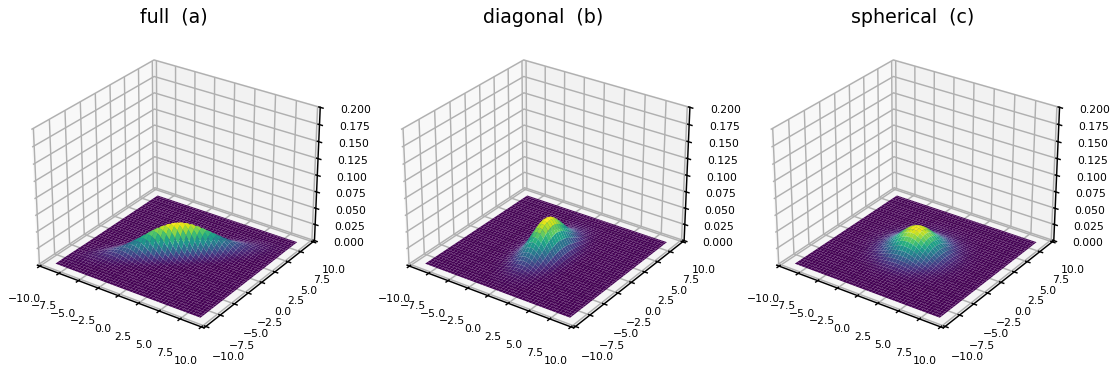
fig_3_5. Download: PDF · PNG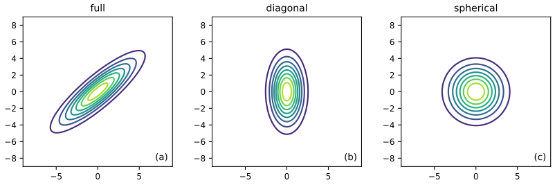
fig_3_6. Download: PDF · SVG3.2.2 Mahalanobis distance
pp. 83–84 The log density is \(\log p(\mathbf{y})=-\tfrac12\Delta^2+\mathrm{const}\) with the squared Mahalanobis distance
\[ \Delta^2=(\mathbf{y}-\boldsymbol\mu)^\T\boldsymbol\Sigma^{-1}(\mathbf{y}-\boldsymbol\mu), \tag{3.20} \]so contours of constant density are contours of constant \(\Delta\).
Result 3.4 (the contours are ellipsoids; the distribution of \(\Delta^2\)) pp. 83–84, (3.21)–(3.25)
With \(\boldsymbol\Sigma=\sum_d\lambda_d\mathbf{u}_d\mathbf{u}_d^\T\) (3.21), \(\boldsymbol\Sigma^{-1}=\sum_d\lambda_d^{-1}\mathbf{u}_d\mathbf{u}_d^\T\) (3.22) and \(z_d=\mathbf{u}_d^\T(\mathbf{y}-\boldsymbol\mu)\),
\[ \Delta^2=\sum_{d=1}^D\frac{z_d^2}{\lambda_d}. \tag{3.24} \](a) The set \(\{\Delta^2=r\}\) is an ellipsoid centred at \(\boldsymbol\mu\) with axes along the eigenvectors \(\mathbf{u}_d\) and semi-axis lengths \(\sqrt{r\lambda_d}\). (b) If \(\mathbf{y}\sim\mathcal N(\boldsymbol\mu,\boldsymbol\Sigma)\) then \(\Delta^2\sim\chi^2_D\); in particular, in two dimensions \(\Pr(\Delta\le k)=1-e^{-k^2/2}\), which is 0.393, 0.865 and 0.989 for \(k=1,2,3\).
Proof
(3.24) follows by inserting (3.22) into (3.20): \((\mathbf{y}-\boldsymbol\mu)^\T\mathbf{u}_d\mathbf{u}_d^\T(\mathbf{y}-\boldsymbol\mu)=z_d^2\). (a) In the orthonormal coordinates \(z_d\), \(\{\sum_dz_d^2/\lambda_d=r\}\) is the axis-aligned ellipsoid with semi-axes \(\sqrt{r\lambda_d}\) along the \(\mathbf{u}_d\): the eigenvectors fix the orientation, the eigenvalues the elongation. (b) By the proof of gap 3.5, \(z_d/\sqrt{\lambda_d}\) are independent \(\mathcal N(0,1)\), and a sum of \(D\) squared independent standard normals is \(\chi^2_D\). For \(D=2\), \(\chi^2_2\) is exponential with mean 2, so \(\Pr(\Delta^2\le k^2)=1-e^{-k^2/2}\). ∎
The demo draws the \(1,2,3\)-standard-deviation ellipses, which therefore contain 39.3%, 86.5% and 98.9% of the mass: in two dimensions "one standard deviation" is a much smaller region than the 68% of the univariate case. Section 7.4.4 of the book returns to the geometry of quadratic forms.
3.2.3 Marginals and conditionals of an MVN
p. 84 Partition \(\mathbf{y}=(\mathbf{y}_1,\mathbf{y}_2)\) with
\[ \boldsymbol\mu=\begin{pmatrix}\boldsymbol\mu_1\\\boldsymbol\mu_2\end{pmatrix},\quad \boldsymbol\Sigma=\begin{pmatrix}\boldsymbol\Sigma_{11}&\boldsymbol\Sigma_{12}\\\boldsymbol\Sigma_{21}&\boldsymbol\Sigma_{22}\end{pmatrix},\quad \boldsymbol\Lambda=\boldsymbol\Sigma^{-1}=\begin{pmatrix}\boldsymbol\Lambda_{11}&\boldsymbol\Lambda_{12}\\\boldsymbol\Lambda_{21}&\boldsymbol\Lambda_{22}\end{pmatrix}. \tag{3.26} \]Result 3.5 (marginals and conditionals of an MVN) p. 84, (3.27)–(3.28)
The marginals are \(p(\mathbf{y}_1)=\mathcal N(\mathbf{y}_1\given\boldsymbol\mu_1,\boldsymbol\Sigma_{11})\) and \(p(\mathbf{y}_2)=\mathcal N(\mathbf{y}_2\given\boldsymbol\mu_2,\boldsymbol\Sigma_{22})\) (3.27). The conditional is \(p(\mathbf{y}_1\given\mathbf{y}_2)=\mathcal N(\mathbf{y}_1\given\boldsymbol\mu_{1|2},\boldsymbol\Sigma_{1|2})\) with
\[ \boldsymbol\mu_{1|2}=\boldsymbol\mu_1+\boldsymbol\Sigma_{12}\boldsymbol\Sigma_{22}^{-1}(\mathbf{y}_2-\boldsymbol\mu_2)=\boldsymbol\mu_1-\boldsymbol\Lambda_{11}^{-1}\boldsymbol\Lambda_{12}(\mathbf{y}_2-\boldsymbol\mu_2)=\boldsymbol\Sigma_{1|2}\big(\boldsymbol\Lambda_{11}\boldsymbol\mu_1-\boldsymbol\Lambda_{12}(\mathbf{y}_2-\boldsymbol\mu_2)\big), \] \[ \boldsymbol\Sigma_{1|2}=\boldsymbol\Sigma_{11}-\boldsymbol\Sigma_{12}\boldsymbol\Sigma_{22}^{-1}\boldsymbol\Sigma_{21}=\boldsymbol\Lambda_{11}^{-1}. \tag{3.28} \]The conditional mean is a linear function of \(\mathbf{y}_2\); the conditional covariance does not depend on \(\mathbf{y}_2\).
Proof (the book defers this to Section 7.3.5)
Step 1: block inverse. Let \(\mathbf{S}=\boldsymbol\Sigma_{11}-\boldsymbol\Sigma_{12}\boldsymbol\Sigma_{22}^{-1}\boldsymbol\Sigma_{21}\) (the Schur complement \(\boldsymbol\Sigma/\boldsymbol\Sigma_{22}\)). Multiplying out confirms the factorisation
\[ \boldsymbol\Sigma=\begin{pmatrix}\mathbf{I}&\boldsymbol\Sigma_{12}\boldsymbol\Sigma_{22}^{-1}\\\mathbf{0}&\mathbf{I}\end{pmatrix}\begin{pmatrix}\mathbf{S}&\mathbf{0}\\\mathbf{0}&\boldsymbol\Sigma_{22}\end{pmatrix}\begin{pmatrix}\mathbf{I}&\mathbf{0}\\\boldsymbol\Sigma_{22}^{-1}\boldsymbol\Sigma_{21}&\mathbf{I}\end{pmatrix}. \]The outer factors have inverses obtained by flipping the sign of the off-diagonal block and have determinant 1, so \(|\boldsymbol\Sigma|=|\mathbf{S}|\,|\boldsymbol\Sigma_{22}|\) and
\[ \boldsymbol\Lambda=\begin{pmatrix}\mathbf{I}&\mathbf{0}\\-\boldsymbol\Sigma_{22}^{-1}\boldsymbol\Sigma_{21}&\mathbf{I}\end{pmatrix}\begin{pmatrix}\mathbf{S}^{-1}&\mathbf{0}\\\mathbf{0}&\boldsymbol\Sigma_{22}^{-1}\end{pmatrix}\begin{pmatrix}\mathbf{I}&-\boldsymbol\Sigma_{12}\boldsymbol\Sigma_{22}^{-1}\\\mathbf{0}&\mathbf{I}\end{pmatrix}. \]Reading off blocks: \(\boldsymbol\Lambda_{11}=\mathbf{S}^{-1}\), \(\boldsymbol\Lambda_{12}=-\mathbf{S}^{-1}\boldsymbol\Sigma_{12}\boldsymbol\Sigma_{22}^{-1}\), \(\boldsymbol\Lambda_{22}=\boldsymbol\Sigma_{22}^{-1}+\boldsymbol\Sigma_{22}^{-1}\boldsymbol\Sigma_{21}\mathbf{S}^{-1}\boldsymbol\Sigma_{12}\boldsymbol\Sigma_{22}^{-1}\). Hence (i) \(\boldsymbol\Lambda_{11}^{-1}=\mathbf{S}\), (ii) \(-\boldsymbol\Lambda_{11}^{-1}\boldsymbol\Lambda_{12}=\boldsymbol\Sigma_{12}\boldsymbol\Sigma_{22}^{-1}\), and (iii) \(\boldsymbol\Lambda_{22}-\boldsymbol\Lambda_{21}\boldsymbol\Lambda_{11}^{-1}\boldsymbol\Lambda_{12}=\boldsymbol\Sigma_{22}^{-1}\) (the second term of \(\boldsymbol\Lambda_{22}\) is exactly \(\boldsymbol\Lambda_{21}\mathbf{S}\boldsymbol\Lambda_{12}\)).
Step 2: conditional. Fix \(\mathbf{y}_2\) and write \(\mathbf{a}=\mathbf{y}_1-\boldsymbol\mu_1\), \(\mathbf{b}=\mathbf{y}_2-\boldsymbol\mu_2\). The exponent of (3.11) is \(-\tfrac12[\mathbf{a}^\T\boldsymbol\Lambda_{11}\mathbf{a}+2\mathbf{a}^\T\boldsymbol\Lambda_{12}\mathbf{b}+\mathbf{b}^\T\boldsymbol\Lambda_{22}\mathbf{b}]\). Complete the square in \(\mathbf{a}\): \[\mathbf{a}^\T\boldsymbol\Lambda_{11}\mathbf{a}+2\mathbf{a}^\T\boldsymbol\Lambda_{12}\mathbf{b}=(\mathbf{a}+\boldsymbol\Lambda_{11}^{-1}\boldsymbol\Lambda_{12}\mathbf{b})^\T\boldsymbol\Lambda_{11}(\mathbf{a}+\boldsymbol\Lambda_{11}^{-1}\boldsymbol\Lambda_{12}\mathbf{b})-\mathbf{b}^\T\boldsymbol\Lambda_{21}\boldsymbol\Lambda_{11}^{-1}\boldsymbol\Lambda_{12}\mathbf{b}\]. So as a function of \(\mathbf{y}_1\), \[p(\mathbf{y}_1,\mathbf{y}_2)\propto\exp[-\tfrac12(\mathbf{y}_1-\boldsymbol\mu_{1|2})^\T\boldsymbol\Lambda_{11}(\mathbf{y}_1-\boldsymbol\mu_{1|2})]\] with \(\boldsymbol\mu_{1|2}=\boldsymbol\mu_1-\boldsymbol\Lambda_{11}^{-1}\boldsymbol\Lambda_{12}\mathbf{b}\), the proportionality constant depending on \(\mathbf{y}_2\) only. A density in \(\mathbf{y}_1\) proportional to a Gaussian kernel is that Gaussian, so \(p(\mathbf{y}_1\given\mathbf{y}_2)=\mathcal N(\boldsymbol\mu_{1|2},\boldsymbol\Lambda_{11}^{-1})\). With (i) and (ii) this gives the first line of (3.28), the second form, and \(\boldsymbol\Sigma_{1|2}=\mathbf{S}\). The third form is \[\boldsymbol\Lambda_{11}^{-1}[\boldsymbol\Lambda_{11}\boldsymbol\mu_1-\boldsymbol\Lambda_{12}\mathbf{b}]=\boldsymbol\mu_1-\boldsymbol\Lambda_{11}^{-1}\boldsymbol\Lambda_{12}\mathbf{b}\].
Step 3: marginal. The leftover factor is \[\exp[-\tfrac12\mathbf{b}^\T(\boldsymbol\Lambda_{22}-\boldsymbol\Lambda_{21}\boldsymbol\Lambda_{11}^{-1}\boldsymbol\Lambda_{12})\mathbf{b}]=\exp[-\tfrac12\mathbf{b}^\T\boldsymbol\Sigma_{22}^{-1}\mathbf{b}]\] by (iii). Integrating the joint over \(\mathbf{y}_1\) multiplies it by the constant \(\int\exp[-\tfrac12(\cdot)]\d\mathbf{y}_1=(2\pi)^{D_1/2}|\mathbf{S}|^{1/2}\) (gap 3.5), so \[p(\mathbf{y}_2)\propto\exp[-\tfrac12(\mathbf{y}_2-\boldsymbol\mu_2)^\T\boldsymbol\Sigma_{22}^{-1}(\mathbf{y}_2-\boldsymbol\mu_2)]\]: a Gaussian with covariance \(\boldsymbol\Sigma_{22}\), whose normalising constant is forced to be \((2\pi)^{D_2/2}|\boldsymbol\Sigma_{22}|^{1/2}\) (consistent with \(|\boldsymbol\Sigma|=|\mathbf{S}||\boldsymbol\Sigma_{22}|\)). The marginal of \(\mathbf{y}_1\) is the same by exchanging the roles of the blocks. ∎
Filling the gap 3.6: what the formulas say, and a numerical confirmation p. 84
Derivation
Information is only added. \(\boldsymbol\Sigma_{11}-\boldsymbol\Sigma_{1|2}=\boldsymbol\Sigma_{12}\boldsymbol\Sigma_{22}^{-1}\boldsymbol\Sigma_{21}\) is positive semidefinite (it has the form \(\mathbf{B}\boldsymbol\Sigma_{22}^{-1}\mathbf{B}^\T\)), so conditioning never increases the covariance in the matrix order. Precision form. The conditional precision \(\boldsymbol\Lambda_{11}\) is simply a block of the joint precision: for conditioning, precision matrices are the convenient parametrisation, for marginalising, covariance matrices are. Independence. \(\boldsymbol\Sigma_{12}=\mathbf{0}\) gives \(\boldsymbol\mu_{1|2}=\boldsymbol\mu_1\), \(\boldsymbol\Sigma_{1|2}=\boldsymbol\Sigma_{11}\): zero cross-covariance means independence for jointly Gaussian blocks (consistent with gap 3.3). Confirmation. For a random \(4\times4\) covariance matrix the three forms of the mean and the two forms of the covariance in (3.28) agree to machine precision, the conditional density equals the joint divided by the marginal at test points, and the conditional mean computed from a slab of simulated samples agrees with (3.28) within sampling error. ∎
3.2.4 Example: conditioning a 2d Gaussian
p. 85 For \(\boldsymbol\Sigma\) as in (3.16) the marginal is \(p(y_1)=\mathcal N(y_1\given\mu_1,\sigma_1^2)\) (3.30), and observing \(Y_2=y_2\) gives
\[ p(y_1\given y_2)=\mathcal N\Big(y_1\,\Big|\,\mu_1+\frac{\rho\sigma_1\sigma_2}{\sigma_2^2}(y_2-\mu_2),\ \sigma_1^2-\frac{(\rho\sigma_1\sigma_2)^2}{\sigma_2^2}\Big). \tag{3.31} \]Filling the gap 3.7: reading (3.31) and (3.32) p. 85
Derivation
(3.31) is (3.28) with \(\boldsymbol\Sigma_{12}=\rho\sigma_1\sigma_2\), \(\boldsymbol\Sigma_{22}=\sigma_2^2\). Simplifying, the conditional mean is \(\mu_1+\rho\frac{\sigma_1}{\sigma_2}(y_2-\mu_2)\) and the conditional variance is \(\sigma_1^2(1-\rho^2)\). Three consequences. (i) The conditional mean is the regression line of \(y_1\) on \(y_2\), with slope \(\rho\sigma_1/\sigma_2=\cov/\mathbb V[Y_2]\) (compare gap 3.2): for Gaussians the best linear predictor is the conditional mean, the best predictor of all. (ii) The variance is reduced by the factor \(1-\rho^2\), whatever the value of \(y_2\): a correlation of 0.8 removes 64% of the variance, one of 0.97 removes 94%. (iii) When \(\sigma_1=\sigma_2=\sigma\) (3.32) the mean moves by \(\rho\) per unit of \(y_2-\mu_2\). With the book's numbers, \(\rho=0.8\), \(\sigma_1=\sigma_2=1\), \(\mu_1=\mu_2=0\), \(y_2=1\): mean 0.8 and variance \(1-0.64=0.36\). ∎
3.2.5 Example: imputing missing values
pp. 85–86 Suppose some coordinates of \(\mathbf{y}\) are observed (indices \(v\), "visible") and the others (indices \(h\), "hidden") are missing. If \(\boldsymbol\theta=(\boldsymbol\mu,\boldsymbol\Sigma)\) is known, (3.28) gives the posterior \(p(\mathbf{y}_h\given\mathbf{y}_v,\boldsymbol\theta)\), and the posterior mean fills the gaps.
Filling the gap 3.8: why the posterior mean is the "best guess" (and what the variance adds) p. 85
The book says the mean "minimizes our expected squared error, as explained in Chapter 5". Here is the one-line argument.
Derivation
For any guess \(\mathbf{g}\) that depends on the observed values only, \[\E[\|\mathbf{y}_h-\mathbf{g}\|^2\given\mathbf{y}_v]=\E[\|\mathbf{y}_h-\bar{\mathbf{y}}_h\|^2\given\mathbf{y}_v]+\|\bar{\mathbf{y}}_h-\mathbf{g}\|^2=\operatorname{tr}\boldsymbol\Sigma_{h|v}+\|\bar{\mathbf{y}}_h-\mathbf{g}\|^2\], where \(\bar{\mathbf{y}}_h=\E[\mathbf{y}_h\given\mathbf{y}_v]\) (the cross term has zero conditional mean). So the posterior mean \(\bar{\mathbf{y}}_h=\boldsymbol\mu_h+\boldsymbol\Sigma_{hv}\boldsymbol\Sigma_{vv}^{-1}(\mathbf{y}_v-\boldsymbol\mu_v)\) minimises the expected squared error, and the minimum is \(\operatorname{tr}\boldsymbol\Sigma_{h|v}\): the posterior covariance is the honest measure of how wrong the guess is, and it depends on which entries are missing but not on the observed values. Multiple imputation draws \(\mathbf{y}_h\) from \(\mathcal N(\bar{\mathbf{y}}_h,\boldsymbol\Sigma_{h|v})\) instead, which keeps the variability that a single filled-in value hides. In the simulation of Figure 3.7 (10 columns, 8 rows, half of the entries hidden) the root mean squared imputation error of the conditional mean is 0.94, against 1.28 for filling with the prior mean 0. ∎
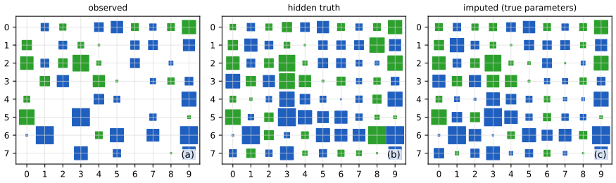
fig_3_7. Download: PDF · SVG3.3 Linear Gaussian systems
p. 86 Section 3.2.3 conditioned on noise-free observations of part of a Gaussian vector. Here the observation is a noisy linear function of the unknown. Let \(\mathbf{z}\in\R^L\) be unknown and \(\mathbf{y}\in\R^D\) a measurement of it, with
\[ p(\mathbf{z})=\mathcal N(\mathbf{z}\given\boldsymbol\mu_z,\boldsymbol\Sigma_z),\qquad p(\mathbf{y}\given\mathbf{z})=\mathcal N(\mathbf{y}\given\mathbf{W}\mathbf{z}+\mathbf{b},\boldsymbol\Sigma_y), \tag{3.33, 3.34} \]where \(\mathbf{W}\) is \(D\times L\). This is a linear Gaussian system. The joint \(p(\mathbf{z},\mathbf{y})=p(\mathbf{z})p(\mathbf{y}\given\mathbf{z})\) is Gaussian in \(\R^{L+D}\) with
\[ \boldsymbol\mu=\begin{pmatrix}\boldsymbol\mu_z\\\mathbf{W}\boldsymbol\mu_z+\mathbf{b}\end{pmatrix},\qquad \boldsymbol\Sigma=\begin{pmatrix}\boldsymbol\Sigma_z&\boldsymbol\Sigma_z\mathbf{W}^\T\\\mathbf{W}\boldsymbol\Sigma_z&\boldsymbol\Sigma_y+\mathbf{W}\boldsymbol\Sigma_z\mathbf{W}^\T\end{pmatrix}. \tag{3.35, 3.36} \]See also (companion course): Bayesian and Probabilistic Machine Learning, Section 2.3.3 (Bayes' theorem for Gaussian variables) and Section 8.1.4 (linear-Gaussian models).
3.3.1 Bayes rule for Gaussians
Result 3.6 (Bayes rule for Gaussians) p. 87, (3.37)–(3.38)
The posterior is \(p(\mathbf{z}\given\mathbf{y})=\mathcal N(\mathbf{z}\given\boldsymbol\mu_{z|y},\boldsymbol\Sigma_{z|y})\) with
\[ \boldsymbol\Sigma_{z|y}^{-1}=\boldsymbol\Sigma_z^{-1}+\mathbf{W}^\T\boldsymbol\Sigma_y^{-1}\mathbf{W},\qquad \boldsymbol\mu_{z|y}=\boldsymbol\Sigma_{z|y}\big[\mathbf{W}^\T\boldsymbol\Sigma_y^{-1}(\mathbf{y}-\mathbf{b})+\boldsymbol\Sigma_z^{-1}\boldsymbol\mu_z\big], \tag{3.37} \]and the normalising constant (the marginal likelihood, or evidence) is
\[ p(\mathbf{y})=\int\mathcal N(\mathbf{z}\given\boldsymbol\mu_z,\boldsymbol\Sigma_z)\,\mathcal N(\mathbf{y}\given\mathbf{W}\mathbf{z}+\mathbf{b},\boldsymbol\Sigma_y)\d\mathbf{z}=\mathcal N(\mathbf{y}\given\mathbf{W}\boldsymbol\mu_z+\mathbf{b},\ \boldsymbol\Sigma_y+\mathbf{W}\boldsymbol\Sigma_z\mathbf{W}^\T). \tag{3.38} \]The Gaussian prior is therefore conjugate to the Gaussian likelihood in \(\mathbf{z}\).
3.3.2 Derivation
Proof of the joint (3.35)–(3.36), of (3.37) by completing the square, and of (3.38)
The joint is Gaussian with mean and covariance (3.35)–(3.36). Write \(\mathbf{y}=\mathbf{W}\mathbf{z}+\mathbf{b}+\boldsymbol\varepsilon\) with \(\boldsymbol\varepsilon\sim\mathcal N(\mathbf{0},\boldsymbol\Sigma_y)\) independent of \(\mathbf{z}\). Then \((\mathbf{z},\mathbf{y})\) is an affine image of the Gaussian vector \((\mathbf{z},\boldsymbol\varepsilon)\), hence Gaussian (the moment generating function \(\E e^{\mathbf{t}^\T(\mathbf{A}\mathbf{x}+\mathbf{c})}\) of an affine image of a Gaussian \(\mathbf{x}\) is again of the Gaussian form). Its mean is \((\boldsymbol\mu_z,\mathbf{W}\boldsymbol\mu_z+\mathbf{b})\); \(\cov[\mathbf{z}]=\boldsymbol\Sigma_z\), \(\cov[\mathbf{z},\mathbf{y}]=\cov[\mathbf{z},\mathbf{W}\mathbf{z}]=\boldsymbol\Sigma_z\mathbf{W}^\T\), and \(\cov[\mathbf{y}]=\mathbf{W}\boldsymbol\Sigma_z\mathbf{W}^\T+\boldsymbol\Sigma_y\) because \(\boldsymbol\varepsilon\) is independent of \(\mathbf{z}\). The \(\mathbf{y}\)-block is the marginal (3.27), which proves (3.38).
(3.37) by completing the square. As a function of \(\mathbf{z}\), the log joint is, up to a constant, \[-\tfrac12(\mathbf{z}-\boldsymbol\mu_z)^\T\boldsymbol\Sigma_z^{-1}(\mathbf{z}-\boldsymbol\mu_z)-\tfrac12(\mathbf{y}-\mathbf{W}\mathbf{z}-\mathbf{b})^\T\boldsymbol\Sigma_y^{-1}(\mathbf{y}-\mathbf{W}\mathbf{z}-\mathbf{b})\] (3.39). Collect terms: this equals \(-\tfrac12\mathbf{z}^\T\mathbf{A}\mathbf{z}+\mathbf{z}^\T\mathbf{c}+\mathrm{const}\) with \(\mathbf{A}=\boldsymbol\Sigma_z^{-1}+\mathbf{W}^\T\boldsymbol\Sigma_y^{-1}\mathbf{W}\) and \(\mathbf{c}=\boldsymbol\Sigma_z^{-1}\boldsymbol\mu_z+\mathbf{W}^\T\boldsymbol\Sigma_y^{-1}(\mathbf{y}-\mathbf{b})\). By the completing-the-square identity (gap 3.9) this is \[-\tfrac12(\mathbf{z}-\mathbf{A}^{-1}\mathbf{c})^\T\mathbf{A}(\mathbf{z}-\mathbf{A}^{-1}\mathbf{c})+\mathrm{const}\]: a Gaussian kernel with covariance \(\mathbf{A}^{-1}=\boldsymbol\Sigma_{z|y}\) and mean \(\mathbf{A}^{-1}\mathbf{c}=\boldsymbol\mu_{z|y}\), which is (3.37). (The book obtains the same result by conditioning the joint with (3.28); the next paragraph shows the two routes agree.)
The two routes agree. Let \(\mathbf{M}=\boldsymbol\Sigma_y+\mathbf{W}\boldsymbol\Sigma_z\mathbf{W}^\T\). Conditioning the joint with (3.28) gives \(\boldsymbol\Sigma_{z|y}=\boldsymbol\Sigma_z-\boldsymbol\Sigma_z\mathbf{W}^\T\mathbf{M}^{-1}\mathbf{W}\boldsymbol\Sigma_z\) and \[\boldsymbol\mu_{z|y}=\boldsymbol\mu_z+\boldsymbol\Sigma_z\mathbf{W}^\T\mathbf{M}^{-1}(\mathbf{y}-\mathbf{W}\boldsymbol\mu_z-\mathbf{b})\]. Multiply the first by \(\mathbf{A}=\boldsymbol\Sigma_z^{-1}+\mathbf{W}^\T\boldsymbol\Sigma_y^{-1}\mathbf{W}\): \(\mathbf{A}\boldsymbol\Sigma_z=\mathbf{I}+\mathbf{W}^\T\boldsymbol\Sigma_y^{-1}\mathbf{W}\boldsymbol\Sigma_z\) and \[\mathbf{A}\boldsymbol\Sigma_z\mathbf{W}^\T=\mathbf{W}^\T+\mathbf{W}^\T\boldsymbol\Sigma_y^{-1}\mathbf{W}\boldsymbol\Sigma_z\mathbf{W}^\T=\mathbf{W}^\T\boldsymbol\Sigma_y^{-1}\mathbf{M}\]. Therefore \[\mathbf{A}\boldsymbol\Sigma_{z|y}=\mathbf{I}+\mathbf{W}^\T\boldsymbol\Sigma_y^{-1}\mathbf{W}\boldsymbol\Sigma_z-\mathbf{W}^\T\boldsymbol\Sigma_y^{-1}\mathbf{M}\mathbf{M}^{-1}\mathbf{W}\boldsymbol\Sigma_z=\mathbf{I}\]: the two covariances coincide (this is the matrix inversion lemma). The same identity, \(\boldsymbol\Sigma_z\mathbf{W}^\T\mathbf{M}^{-1}=\boldsymbol\Sigma_{z|y}\mathbf{W}^\T\boldsymbol\Sigma_y^{-1}\), turns the conditioning mean into \(\boldsymbol\mu_z+\boldsymbol\Sigma_{z|y}\mathbf{W}^\T\boldsymbol\Sigma_y^{-1}(\mathbf{y}-\mathbf{b}-\mathbf{W}\boldsymbol\mu_z)\), and since \(\boldsymbol\Sigma_{z|y}\mathbf{A}=\mathbf{I}\) gives \[\boldsymbol\mu_z-\boldsymbol\Sigma_{z|y}\mathbf{W}^\T\boldsymbol\Sigma_y^{-1}\mathbf{W}\boldsymbol\mu_z=\boldsymbol\Sigma_{z|y}\boldsymbol\Sigma_z^{-1}\boldsymbol\mu_z\], this is exactly (3.37). The identity of the two routes was also confirmed numerically on random systems. ∎
Filling the gap 3.9: completing the square p. 88
The book states the scalar and vector identities without proof.
Derivation
Scalar. \[a(x-h)^2+k=ax^2-2ahx+ah^2+k\]. Matching coefficients with \(ax^2+bx+c\) gives \(-2ah=b\), so \(h=-b/(2a)\), and \(ah^2+k=c\), so \(k=c-ah^2=c-b^2/(4a)\). Vector. For symmetric \(\mathbf{A}\) (positive definite when used for a Gaussian), \[(\mathbf{x}-\mathbf{h})^\T\mathbf{A}(\mathbf{x}-\mathbf{h})+k=\mathbf{x}^\T\mathbf{A}\mathbf{x}-2\mathbf{h}^\T\mathbf{A}\mathbf{x}+\mathbf{h}^\T\mathbf{A}\mathbf{h}+k\]; matching with \(\mathbf{x}^\T\mathbf{A}\mathbf{x}+\mathbf{x}^\T\mathbf{b}+c\) needs \(-2\mathbf{A}\mathbf{h}=\mathbf{b}\), i.e. \(\mathbf{h}=-\tfrac12\mathbf{A}^{-1}\mathbf{b}\), and \(k=c-\mathbf{h}^\T\mathbf{A}\mathbf{h}=c-\tfrac14\mathbf{b}^\T\mathbf{A}^{-1}\mathbf{b}\). In the proof of Result 3.6 the quadratic is \(-\tfrac12\mathbf{z}^\T\mathbf{A}\mathbf{z}+\mathbf{z}^\T\mathbf{c}\), i.e. the vector identity with \(\mathbf{A}\to-\tfrac12\mathbf{A}\), \(\mathbf{b}\to\mathbf{c}\), whose centre is \(\mathbf{h}=\mathbf{A}^{-1}\mathbf{c}\). ∎
3.3.3 Example: inferring an unknown scalar
pp. 88–90 Take \(N\) measurements \(y_i\sim\mathcal N(z,\lambda_y^{-1})\) of a scalar \(z\) with known noise precision \(\lambda_y=1/\sigma^2\) and prior \(\mathcal N(z\given\mu_0,\lambda_0^{-1})\). Stacking \(\mathbf{y}=(y_1,\dots,y_N)\), \(\mathbf{W}=\mathbf{1}_N\), \(\boldsymbol\Sigma_y^{-1}=\lambda_y\mathbf{I}\), Result 3.6 gives
\[ p(z\given\mathbf{y})=\mathcal N(z\given\mu_N,\lambda_N^{-1}),\qquad \lambda_N=\lambda_0+N\lambda_y,\qquad \mu_N=\frac{N\lambda_y\bar y+\lambda_0\mu_0}{\lambda_N}=\frac{N\lambda_y}{N\lambda_y+\lambda_0}\bar y+\frac{\lambda_0}{N\lambda_y+\lambda_0}\mu_0. \tag{3.52–3.54} \]In terms of variances, with \(\tau_0^2=1/\lambda_0\) and \(\tau_N^2=1/\lambda_N\) (3.55–3.57): \(\tau_N^2=\big(\tfrac N{\sigma^2}+\tfrac1{\tau_0^2}\big)^{-1}=\tfrac{\sigma^2\tau_0^2}{N\tau_0^2+\sigma^2}\), \(\mu_N=\tfrac{\sigma^2}{N\tau_0^2+\sigma^2}\mu_0+\tfrac{N\tau_0^2}{N\tau_0^2+\sigma^2}\bar y\).
Filling the gap 3.10: the three forms of the posterior mean, sequential updating, shrinkage and the signal-to-noise ratio pp. 89–90, (3.58)–(3.64)
Derivation
Where (3.52)–(3.54) come from. Apply (3.37) with \(\boldsymbol\Sigma_z=\lambda_0^{-1}\), \(\mathbf{W}^\T\boldsymbol\Sigma_y^{-1}\mathbf{W}=\lambda_y\mathbf{1}^\T\mathbf{1}=N\lambda_y\), and \(\mathbf{W}^\T\boldsymbol\Sigma_y^{-1}\mathbf{y}=\lambda_y\sum_iy_i=N\lambda_y\bar y\). Interpretation. Precisions add: the posterior precision is the prior precision plus \(N\) units of measurement precision. The mean is a convex combination of \(\bar y\) (the MLE) and \(\mu_0\) with weights proportional to the two precisions, \(N\lambda_y\) and \(\lambda_0\); as \(N\to\infty\) the weight on the prior goes to 0 and the posterior concentrates at \(\bar y\).
Three forms (3.61)–(3.63). For one observation write the likelihood, prior and posterior variances as \(\Sigma_y,\Sigma_0,\Sigma_1\), so \(\Sigma_1=\Sigma_0\Sigma_y/(\Sigma_0+\Sigma_y)\) (3.59) and \(\mu_1=\Sigma_1(\mu_0/\Sigma_0+y/\Sigma_y)\) (3.60). Then \(\mu_1=\frac{\Sigma_y}{\Sigma_0+\Sigma_y}\mu_0+\frac{\Sigma_0}{\Sigma_0+\Sigma_y}y\) (3.61). Rewriting \(\frac{\Sigma_y}{\Sigma_0+\Sigma_y}=1-\frac{\Sigma_0}{\Sigma_0+\Sigma_y}\) gives \(\mu_1=\mu_0+(y-\mu_0)\frac{\Sigma_0}{\Sigma_0+\Sigma_y}\) (3.62): the prior mean moved towards the data by the fraction \(\Sigma_0/(\Sigma_0+\Sigma_y)\) of the gap. Rewriting \(\frac{\Sigma_0}{\Sigma_0+\Sigma_y}=1-\frac{\Sigma_y}{\Sigma_0+\Sigma_y}\) gives \(\mu_1=y-(y-\mu_0)\frac{\Sigma_y}{\Sigma_0+\Sigma_y}\) (3.63): the datum pulled back towards the prior mean, which is called shrinkage, by the fraction \(\Sigma_y/(\Sigma_0+\Sigma_y)\). A strong prior (\(\Sigma_0\) small relative to \(\Sigma_y\)) shrinks a lot; a weak prior hardly at all (Figure 3.8).
Sequential equals batch. Updating after each observation with the one-observation formulas, the precision after \(n\) points is \(\lambda_0+n\lambda_y\) and the precision-weighted sum \(\lambda_n\mu_n=\lambda_0\mu_0+\lambda_y\sum_{i\le n}y_i\) increases by \(\lambda_yy_n\) at step \(n\); at \(n=N\) these are \(\lambda_N\) and \(\lambda_N\mu_N\) of (3.53)–(3.54). So the order of the data is irrelevant and one may update point by point or all at once (confirmed numerically).
Signal-to-noise ratio (3.64). With \(z\sim\mathcal N(\mu_0,\Sigma_0)\), \(y=z+\epsilon\), \(\epsilon\sim\mathcal N(0,\Sigma_y)\) independent: \(\mathrm{SNR}=\E[z^2]/\E[\epsilon^2]=(\Sigma_0+\mu_0^2)/\Sigma_y\), using \(\E z^2=\mathbb V[z]+(\E z)^2\). For \(\mu_0=0\) it is \(\Sigma_0/\Sigma_y\), and the data weight in (3.61) is \(\mathrm{SNR}/(1+\mathrm{SNR})\): high signal-to-noise ratio, little shrinkage. Variance never exceeds either source: \(\Sigma_1^{-1}=\Sigma_0^{-1}+\Sigma_y^{-1}\) exceeds both, so \(\Sigma_1\lt\min(\Sigma_0,\Sigma_y)\). ∎
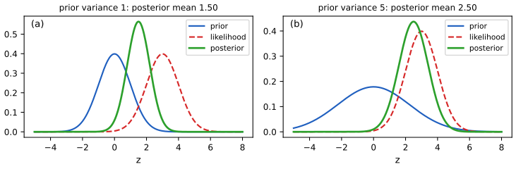
fig_3_8. Download: PDF · SVG3.3.4 Example: inferring an unknown vector
pp. 90–92 Now \(\mathbf{z}\in\R^D\) with prior \(\mathcal N(\boldsymbol\mu_z,\boldsymbol\Sigma_z)\), observed through \(N\) independent measurements \(\mathbf{y}_n\sim\mathcal N(\mathbf{z},\boldsymbol\Sigma_y)\). The book claims that the likelihood of \(N\) points is proportional to a single Gaussian at their average,
\[ p(\mathcal D\given\mathbf{z})=\prod_{n=1}^N\mathcal N(\mathbf{y}_n\given\mathbf{z},\boldsymbol\Sigma_y)\ \propto\ \mathcal N\big(\bar{\mathbf{y}}\,\big|\,\mathbf{z},\tfrac1N\boldsymbol\Sigma_y\big), \tag{3.65} \]and then \(p(\mathbf{z}\given\mathcal D)=\mathcal N(\mathbf{z}\given\hat{\boldsymbol\mu},\hat{\boldsymbol\Sigma})\) with \(\hat{\boldsymbol\Sigma}^{-1}=\boldsymbol\Sigma_z^{-1}+N\boldsymbol\Sigma_y^{-1}\) and \(\hat{\boldsymbol\mu}=\hat{\boldsymbol\Sigma}(\boldsymbol\Sigma_y^{-1}N\bar{\mathbf{y}}+\boldsymbol\Sigma_z^{-1}\boldsymbol\mu_z)\) (3.66–3.68).
Filling the gap 3.11: the sample mean is sufficient (3.65), for any number of points p. 91
The book verifies (3.65) for two points by expanding. Here is the argument for \(N\) points, which also shows where the constant is.
Derivation
Write \(\mathbf{P}=\boldsymbol\Sigma_y^{-1}\). In \(\mathbf{y}_n-\mathbf{z}=(\mathbf{y}_n-\bar{\mathbf{y}})+(\bar{\mathbf{y}}-\mathbf{z})\), expand the quadratic form and sum over \(n\):
\[ \sum_n(\mathbf{y}_n-\mathbf{z})^\T\mathbf{P}(\mathbf{y}_n-\mathbf{z})=\sum_n(\mathbf{y}_n-\bar{\mathbf{y}})^\T\mathbf{P}(\mathbf{y}_n-\bar{\mathbf{y}})+N(\bar{\mathbf{y}}-\mathbf{z})^\T\mathbf{P}(\bar{\mathbf{y}}-\mathbf{z}), \]because the cross term \(2\sum_n(\mathbf{y}_n-\bar{\mathbf{y}})^\T\mathbf{P}(\bar{\mathbf{y}}-\mathbf{z})\) vanishes (\(\sum_n(\mathbf{y}_n-\bar{\mathbf{y}})=\mathbf{0}\)). The first term does not involve \(\mathbf{z}\). Hence \[\prod_n\mathcal N(\mathbf{y}_n\given\mathbf{z},\boldsymbol\Sigma_y)=C(\mathcal D)\,\exp[-\tfrac N2(\bar{\mathbf{y}}-\mathbf{z})^\T\mathbf{P}(\bar{\mathbf{y}}-\mathbf{z})]\], and \[\exp[-\tfrac12(\bar{\mathbf{y}}-\mathbf{z})^\T(N\mathbf{P})(\bar{\mathbf{y}}-\mathbf{z})]\propto\mathcal N(\bar{\mathbf{y}}\given\mathbf{z},\boldsymbol\Sigma_y/N)\] as a function of \(\mathbf{z}\): (3.65), with a proportionality constant that depends on the data only. Constants in \(\mathbf{z}\) cancel in Bayes' rule, so the posterior can be computed from \(\bar{\mathbf{y}}\) alone: the sample mean is a sufficient statistic for \(\mathbf{z}\) here. Applying Result 3.6 with \(\mathbf{W}=\mathbf{I}\), \(\mathbf{b}=\mathbf{0}\) and noise covariance \(\boldsymbol\Sigma_y/N\) gives (3.66–3.68). The same answer is obtained from the stacked system with \(\mathbf{W}=[\mathbf{I};\dots;\mathbf{I}]\) and block-diagonal noise (confirmed numerically). Flat prior. Letting \(\boldsymbol\Sigma_z^{-1}\to\mathbf{0}\) gives \(\hat{\boldsymbol\mu}=\bar{\mathbf{y}}\) and \(\hat{\boldsymbol\Sigma}=\boldsymbol\Sigma_y/N\), the sampling distribution of the average. Direction dependence. The posterior is wider along directions in which the sensor is noisier (the axis along \(y_1\) in Figure 3.9). ∎
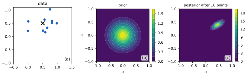
fig_3_9. Download: PDF · SVG3.3.5 Example: sensor fusion
pp. 92–93 With \(M\) sensors, the \(m\)-th giving \(N_m\) readings \(\mathbf{y}_{n,m}\sim\mathcal N(\mathbf{z},\boldsymbol\Sigma_m)\), the model is \[p(\mathbf{z},\mathbf{y})=p(\mathbf{z})\prod_m\prod_n\mathcal N(\mathbf{y}_{n,m}\given\mathbf{z},\boldsymbol\Sigma_m)\] (3.69). The posterior \(p(\mathbf{z}\given\mathbf{y})\) is the sensor fusion of the readings.
Filling the gap 3.12: fusion is precision weighting (general case, and Exercise 3.7) pp. 92–93, Exercise 3.7
Derivation
General formula. Each reading enters the log posterior through \(-\tfrac12(\mathbf{y}_{n,m}-\mathbf{z})^\T\boldsymbol\Sigma_m^{-1}(\mathbf{y}_{n,m}-\mathbf{z})\), a quadratic in \(\mathbf{z}\) with matrix \(\boldsymbol\Sigma_m^{-1}\) and linear term \(\boldsymbol\Sigma_m^{-1}\mathbf{y}_{n,m}\). Adding the prior and completing the square (gap 3.9), the posterior is Gaussian with
\[ \boldsymbol\Sigma_{z|y}^{-1}=\boldsymbol\Sigma_z^{-1}+\sum_mN_m\boldsymbol\Sigma_m^{-1},\qquad \boldsymbol\mu_{z|y}=\boldsymbol\Sigma_{z|y}\Big[\boldsymbol\Sigma_z^{-1}\boldsymbol\mu_z+\sum_m\boldsymbol\Sigma_m^{-1}\sum_n\mathbf{y}_{n,m}\Big]. \]With a flat prior and \(N_m=1\) (the two-sensor case of the book, equivalent to \(\mathbf{W}=[\mathbf{I};\mathbf{I}]\) and \(\boldsymbol\Sigma_y=\diag(\boldsymbol\Sigma_1,\boldsymbol\Sigma_2)\)): \(\boldsymbol\Sigma_{z|y}=(\boldsymbol\Sigma_1^{-1}+\boldsymbol\Sigma_2^{-1})^{-1}\) and \(\boldsymbol\mu_{z|y}=\boldsymbol\Sigma_{z|y}(\boldsymbol\Sigma_1^{-1}\mathbf{y}_1+\boldsymbol\Sigma_2^{-1}\mathbf{y}_2)\): a matrix-weighted average of the readings, the weights \(\boldsymbol\Sigma_{z|y}\boldsymbol\Sigma_m^{-1}\) summing to \(\mathbf{I}\).
The three cases of Figure 3.10. (a) \(\boldsymbol\Sigma_1=\boldsymbol\Sigma_2=0.01\mathbf{I}\): weights \(\tfrac12\) each, mean \((0.5,-0.5)\), the midpoint of \(\mathbf{y}_1=(0,-1)\) and \(\mathbf{y}_2=(1,0)\), posterior covariance \(0.005\mathbf{I}\). (b) \(\boldsymbol\Sigma_1=0.05\mathbf{I}\), \(\boldsymbol\Sigma_2=0.01\mathbf{I}\): precisions 20 and 100, weights \(\tfrac16,\tfrac56\), mean \(\tfrac16(0,-1)+\tfrac56(1,0)=(0.833,-0.167)\). (c) With \(\boldsymbol\Sigma_1=0.01\begin{pmatrix}10&1\\1&1\end{pmatrix}\), \(\boldsymbol\Sigma_2=0.01\begin{pmatrix}1&1\\1&10\end{pmatrix}\) (3.70), each sensor is precise in one coordinate and the matrix weights pick that coordinate from each sensor: the mean is \((0.846,-0.846)\), close to (the horizontal coordinate of \(\mathbf{y}_2\), the vertical coordinate of \(\mathbf{y}_1\)). These were computed numerically and agree with the formulas.
Exercise 3.7 (one dimension). With \(n_1\) readings of variance \(v_1\) and \(n_2\) of variance \(v_2\) and a flat prior (precision 0), \(\mu\given\mathcal D\sim\mathcal N(m,s^2)\) with
\[ s^2=\Big(\frac{n_1}{v_1}+\frac{n_2}{v_2}\Big)^{-1},\qquad m=s^2\Big(\frac{n_1\bar y^{(1)}}{v_1}+\frac{n_2\bar y^{(2)}}{v_2}\Big), \]by the formula above with \(D=1\) (the sum of readings from sensor \(m\) is \(n_m\bar y^{(m)}\)). The precise digital sensor (small \(v_1\)) dominates the mercury thermometer unless the latter has many more readings: each reading is worth \(1/v\) units of information. ∎
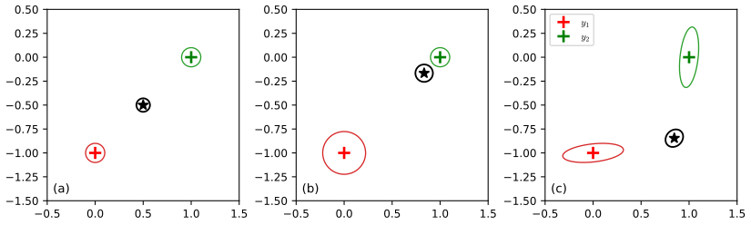
fig_3_10. Download: PDF · SVG3.4 The exponential family
p. 93 The exponential family contains most of the distributions used in this book (Gaussian, Bernoulli, categorical, Poisson, gamma, beta, Dirichlet, ...). Its main use here is to define generalised linear models (Chapter 12).
See also (companion course): Bayesian and Probabilistic Machine Learning, Section 2.4 (the exponential family, maximum likelihood and conjugate priors).
3.4.1 Definition
Definition 3.4 (exponential family) pp. 93–94, (3.71)–(3.73)
A family of densities (or mass functions) on a fixed support, indexed by \(\boldsymbol\eta\in\R^K\), is an exponential family if
\[ p(\mathbf{y}\given\boldsymbol\eta)=\frac{1}{Z(\boldsymbol\eta)}h(\mathbf{y})\exp\big[\boldsymbol\eta^\T\mathcal T(\mathbf{y})\big]=h(\mathbf{y})\exp\big[\boldsymbol\eta^\T\mathcal T(\mathbf{y})-A(\boldsymbol\eta)\big], \tag{3.71} \]with base measure \(h\), sufficient statistics \(\mathcal T(\mathbf{y})\in\R^K\), natural (canonical) parameters \(\boldsymbol\eta\), partition function \(Z\) and log partition function \(A=\log Z\). The natural parameter space is \(\Omega=\{\boldsymbol\eta:A(\boldsymbol\eta)\lt \infty\}\). If \(\boldsymbol\eta=f(\boldsymbol\phi)\) for a smaller parameter \(\boldsymbol\phi\) (3.72) the family is curved when \(f\) is nonlinear; with \(\mathcal T(\mathbf{y})=\mathbf{y}\) it is a natural exponential family (3.73).
Correction to the book: the definition of a minimal representation
The book (p. 93) calls the family minimal if "there is no \(\boldsymbol\eta\in\R^K\setminus\{\mathbf{0}\}\) such that \(\boldsymbol\eta^\T\mathcal T(\mathbf{y})=0\)". With that wording the over-complete Bernoulli representation of (3.74)–(3.77), \(\mathcal T(y)=[\mathbb I(y=1),\mathbb I(y=0)]\), would count as minimal: \(\eta_1\mathbb I(y=1)+\eta_2\mathbb I(y=0)=0\) for \(y=0\) and \(y=1\) forces \(\eta_1=\eta_2=0\). Yet the book (correctly) calls it over-complete because \(\mathbf{1}^\T\mathcal T(y)=1\). The right condition is that no \(\boldsymbol\eta\ne\mathbf{0}\) makes \(\boldsymbol\eta^\T\mathcal T(\mathbf{y})\) constant (almost everywhere in the support): then \(\mathbf{1}\) is such a vector for the over-complete form, and none exists for \(\mathcal T(y)=y\). Equivalently, the covariance matrix of \(\mathcal T\) is positive definite, which is what is needed in Result 3.7.
3.4.2 Example
p. 94 The Bernoulli distribution \(\operatorname{Ber}(y\given\mu)=\mu^y(1-\mu)^{1-y}\) can be written as \(\exp[y\log\tfrac\mu{1-\mu}+\log(1-\mu)]\) (3.78), i.e. in the form (3.71) with
\[ \eta=\log\frac{\mu}{1-\mu},\quad \mathcal T(y)=y,\quad h(y)=1,\quad A(\eta)=-\log(1-\mu)=\log(1+e^\eta),\qquad \mu=\sigma(\eta)=\frac1{1+e^{-\eta}}. \tag{3.79–3.83} \]To see the last one, \[\eta=\log\frac\mu{1-\mu}\Rightarrow e^\eta=\frac\mu{1-\mu}\Rightarrow\mu=\frac{e^\eta}{1+e^\eta}\]; and \(1-\mu=\frac1{1+e^\eta}\), so \(-\log(1-\mu)=\log(1+e^\eta)\). So the sigmoid is the map from natural parameter to mean parameter, and the derivative of \(A\) is the mean: \(A'(\eta)=\frac{e^\eta}{1+e^\eta}=\mu=\E[y]\), the first instance of the next result.
3.4.3 Log partition function is cumulant generating function
Result 3.7 (properties of \(A\)) pp. 95, (3.84)–(3.85)
(a) \(\Omega\) is convex and \(A\) is convex on it. (b) In the interior of \(\Omega\), \(A\) is infinitely differentiable, with
\[ \nabla A(\boldsymbol\eta)=\E[\mathcal T(\mathbf{y})],\qquad \nabla^2A(\boldsymbol\eta)=\cov[\mathcal T(\mathbf{y})]. \tag{3.84, 3.85} \](c) \(\nabla^2A\) is positive definite for all \(\boldsymbol\eta\) in the interior of \(\Omega\) exactly when the representation is minimal (in the corrected sense above); then \(A\) is strictly convex. (d) For \(N\) iid observations the log likelihood \[\ell(\boldsymbol\eta)=\boldsymbol\eta^\T\sum_n\mathcal T(\mathbf{y}_n)-NA(\boldsymbol\eta)+\mathrm{const}\] is concave; a maximiser \(\hat{\boldsymbol\eta}\) in the interior satisfies the moment-matching condition \(\nabla A(\hat{\boldsymbol\eta})=\frac1N\sum_n\mathcal T(\mathbf{y}_n)\), and is unique when the representation is minimal.
Proof
(a) Write \(Z(\boldsymbol\eta)=\int h(\mathbf{y})e^{\boldsymbol\eta^\T\mathcal T(\mathbf{y})}\d\mathbf{y}\) (a sum for discrete \(\mathbf{y}\)). For \(\boldsymbol\eta_1,\boldsymbol\eta_2\in\Omega\) and \(\theta\in(0,1)\), Hölder's inequality with exponents \(1/\theta\) and \(1/(1-\theta)\) applied to \(f_1=he^{\theta\boldsymbol\eta_1^\T\mathcal T}\) and \(f_2=he^{(1-\theta)\boldsymbol\eta_2^\T\mathcal T}\) (with \(h=h^\theta h^{1-\theta}\)) gives \[Z(\theta\boldsymbol\eta_1+(1-\theta)\boldsymbol\eta_2)\le Z(\boldsymbol\eta_1)^\theta Z(\boldsymbol\eta_2)^{1-\theta}\lt \infty\]. So \(\Omega\) is convex, and taking logarithms, \[A(\theta\boldsymbol\eta_1+(1-\theta)\boldsymbol\eta_2)\le\theta A(\boldsymbol\eta_1)+(1-\theta)A(\boldsymbol\eta_2)\]: \(A\) is convex.
(b) In the interior of \(\Omega\), \(\int h\,e^{\boldsymbol\eta^\T\mathcal T}\,\|\mathcal T\|^k\d\mathbf{y}\lt \infty\) for every \(k\) (move \(\boldsymbol\eta\) a little in the direction of each coordinate and use \(\|t\|^k\le C_\varepsilon e^{\varepsilon\|t\|}\)), so differentiation under the integral sign is justified by dominated convergence, and \(Z\) is smooth. Then \[\nabla A=\nabla Z/Z=\int\mathcal T\,he^{\boldsymbol\eta^\T\mathcal T}\d\mathbf{y}/Z=\E[\mathcal T]\], and \[\nabla^2A=\nabla^2Z/Z-(\nabla Z/Z)(\nabla Z/Z)^\T=\E[\mathcal T\mathcal T^\T]-\E[\mathcal T]\E[\mathcal T]^\T=\cov[\mathcal T]\].
(c) For a vector \(\mathbf{v}\), \(\mathbf{v}^\T\nabla^2A\,\mathbf{v}=\mathbb V[\mathbf{v}^\T\mathcal T(\mathbf{y})]\ge0\), which is 0 for some \(\mathbf{v}\ne\mathbf{0}\) iff \(\mathbf{v}^\T\mathcal T\) is almost surely constant, i.e. iff the representation is not minimal. (So "the Hessian is positive definite" in the book needs minimality; in general it is positive semidefinite, which still gives convexity.)
(d) \(\ell\) is linear minus \(NA\), so concave by (a), strictly if \(A\) is strictly convex. Setting \(\nabla\ell=\sum_n\mathcal T(\mathbf{y}_n)-N\nabla A=0\) gives the stated condition. For a concave differentiable function, a stationary point is a global maximiser; strict concavity gives uniqueness. ∎
Check on the Bernoulli family: \(A(\eta)=\log(1+e^\eta)\) gives \(A'=\sigma(\eta)=\mu\) and \[A''=\sigma(\eta)(1-\sigma(\eta))=\mu(1-\mu)=\mathbb V[y]\]. Numerical differentiation of \(A\) for the Poisson (\(A=e^\eta\), mean and variance both \(e^\eta\)), gamma with known shape \(k\) (\(A=-k\log(-\eta)\)) and Gaussian families gives the same means and covariances as the formulas.
3.4.4 Maximum entropy derivation of the exponential family
pp. 95–96 Suppose all we know of a distribution on a discrete set is the expected values \(F_k\) of features \(f_k\): \(\sum_xp(x)f_k(x)=F_k\) (3.86). Among all \(p\) satisfying this, choose the one closest, in Kullback–Leibler divergence, to a reference distribution \(q\):
\[ \min_p\ \KL(p\,\|\,q)\quad\text{subject to the constraints and}\ \sum_xp(x)=1. \tag{3.87} \]For uniform \(q\) this is maximising the entropy \(H(p)\) (3.88). The book uses Lagrange multipliers (3.89–3.90) and obtains \(p(x)=\frac1Zq(x)\exp[-\sum_k\lambda_kf_k(x)]\) (3.91), with \(Z=\sum_xq(x)\exp[-\sum_k\lambda_kf_k(x)]\) (3.93): an exponential family with sufficient statistics \(f(x)\), natural parameters \(-\boldsymbol\lambda\) and base measure \(q\).
Result 3.8 (the exponential form is the minimiser, not merely a stationary point) p. 96
Suppose \(p^\star(x)=q(x)e^{-\boldsymbol\lambda^\T\mathbf{f}(x)}/Z\) satisfies the constraints (3.86). Then every \(p\) satisfying them has \(\KL(p\|q)\ge\KL(p^\star\|q)\), with equality only for \(p=p^\star\).
Proof
The Lagrange argument finds where the derivative vanishes; it does not show the point is a minimum. Here is the direct argument (Gibbs' inequality). For any feasible \(p\), \[\KL(p\|q)-\KL(p\|p^\star)=\sum_xp\log\frac{p^\star}{q}=\sum_xp(x)\big[-\boldsymbol\lambda^\T\mathbf{f}(x)-\log Z\big]=-\boldsymbol\lambda^\T\mathbf{F}-\log Z\], which does not depend on \(p\) because \(p\) satisfies the constraints. The same holds for \(p^\star\) (it is feasible, and \(\KL(p^\star\|p^\star)=0\)): \(\KL(p^\star\|q)=-\boldsymbol\lambda^\T\mathbf{F}-\log Z\). Subtracting, \[\KL(p\|q)-\KL(p^\star\|q)=\KL(p\|p^\star)\ge0\], with equality iff \(p=p^\star\). ∎
Gaussian as a maximum entropy distribution. With \(f_1(x)=x\), \(f_2(x)=x^2\) and a uniform (flat) \(q\) on \(\R\) (the argument is the same with sums replaced by integrals), \(p^\star\propto\exp[-\lambda_1x-\lambda_2x^2]\), a Gaussian when \(\lambda_2>0\), with the prescribed mean and variance; by Result 3.8 (continuous version, where the KL to the flat measure is minus the differential entropy), it has the largest differential entropy among all densities with that mean and variance. This is a numerical fact one can see by comparing entropies at equal variance: for variance \(1.3^2\), the Gaussian has entropy 1.681 nats, a Laplace density 1.609 and a uniform density 1.505 (rounded; the exact values are \(\tfrac12\log(2\pi e\sigma^2)\), \(1+\log(2b)\) with \(b=\sigma/\sqrt2\), and \(\log(2\sqrt3\sigma)\)). The discrete case, a distribution on \(\{0,\dots,5\}\) with a prescribed mean, was solved by a constrained optimiser and agrees with the exponential form \(p(x)\propto e^{-\lambda x}\).
3.5 Mixture models
p. 96 A mixture model is a convex combination of simple distributions,
\[ p(\mathbf{y}\given\boldsymbol\theta)=\sum_{k=1}^K\pi_kp_k(\mathbf{y}),\qquad 0\le\pi_k\le1,\ \ \sum_k\pi_k=1. \tag{3.94} \]Equivalently, a hierarchical model with a discrete latent variable \(z\in\{1,\dots,K\}\): \(p(z\given\boldsymbol\theta)=\operatorname{Cat}(z\given\boldsymbol\pi)\), \(p(\mathbf{y}\given z=k,\boldsymbol\theta)=p(\mathbf{y}\given\boldsymbol\theta_k)\) (3.95–3.96). First sample a component, then sample from it; summing out \(z\) recovers (3.94) (3.97), since \[\sum_kp(z=k)p(\mathbf{y}\given z=k)=\sum_k\pi_kp_k(\mathbf{y})\].
See also (companion course): Section 2.3.9 (mixtures of Gaussians), Chapter 9 (EM for mixtures, with the full derivation) and the K-means and EM demo.
3.5.1 Gaussian mixture models
pp. 97–98 A Gaussian mixture model (GMM) takes \(p_k=\mathcal N(\boldsymbol\mu_k,\boldsymbol\Sigma_k)\):
\[ p(\mathbf{y}\given\boldsymbol\theta)=\sum_{k=1}^K\pi_k\,\mathcal N(\mathbf{y}\given\boldsymbol\mu_k,\boldsymbol\Sigma_k). \tag{3.98} \]Used for clustering, one first fits \(\hat{\boldsymbol\theta}=\arg\max\log p(\mathcal D\given\boldsymbol\theta)\) (by EM, Section 8.7.3 of the book), then computes for each point the responsibility of each cluster
\[ r_{nk}=p(z_n=k\given\mathbf{y}_n,\boldsymbol\theta)=\frac{\pi_kp(\mathbf{y}_n\given\boldsymbol\theta_k)}{\sum_{k'}\pi_{k'}p(\mathbf{y}_n\given\boldsymbol\theta_{k'})}, \tag{3.99} \]and the hard assignment \[\hat z_n=\arg\max_kr_{nk}=\arg\max_k[\log p(\mathbf{y}_n\given z_n=k,\boldsymbol\theta)+\log\pi_k]\] (3.100).
Filling the gap 3.13: mixture moments, responsibilities and the K-means limit (3.101) pp. 96–98
Derivation
Mean and covariance of a mixture. If \(\mathbf{y}\) has density (3.94) with component means \(\boldsymbol\mu_k\) and covariances \(\boldsymbol\Sigma_k\), the laws of total expectation and covariance (condition on \(z\)) give
\[ \E\mathbf{y}=\sum_k\pi_k\boldsymbol\mu_k=:\bar{\boldsymbol\mu},\qquad \cov[\mathbf{y}]=\sum_k\pi_k\big(\boldsymbol\Sigma_k+\boldsymbol\mu_k\boldsymbol\mu_k^\T\big)-\bar{\boldsymbol\mu}\bar{\boldsymbol\mu}^\T. \](The first is \(\E[\E[\mathbf{y}\given z]]\); the second is \(\E[\mathbf{y}\mathbf{y}^\T]=\E[\boldsymbol\Sigma_z+\boldsymbol\mu_z\boldsymbol\mu_z^\T]\) from (3.4) applied within each component.) So the mixture covariance is the average within-component covariance plus the covariance of the component means: a mixture of Gaussians is generally not Gaussian but its first two moments are explicit. Confirmed by simulation for the mixture of Figure 3.11.
Responsibilities. (3.99) is Bayes' rule for the latent \(z_n\) with prior \(\pi_k\) and likelihood \(p(\mathbf{y}_n\given\theta_k)\); the responsibilities of a point sum to 1 over \(k\). In (3.100) the denominator of (3.99) is the same for all \(k\) and the logarithm is increasing, hence the second form.
K-means limit (3.101). If \(\pi_k=1/K\) and \(\boldsymbol\Sigma_k=\mathbf{I}\), then \[\log p(\mathbf{y}\given z=k)+\log\pi_k=-\tfrac12\|\mathbf{y}-\boldsymbol\mu_k\|^2-\tfrac D2\log2\pi-\log K\], and only the first term depends on \(k\): \(\hat z_n=\arg\min_k\|\mathbf{y}_n-\boldsymbol\mu_k\|^2\), assignment to the nearest centroid. (Without the uniform weights the log prior \(\log\pi_k\) shifts the boundary towards the heavier component. As the common covariance \(\sigma^2\mathbf{I}\) shrinks to 0 with the means fixed, the soft responsibilities themselves become 0/1 and the soft clustering becomes hard, which is how K-means arises as a limit of EM.) Numerically, with random centroids and 500 test points, the arg max of the GMM responsibilities coincides with the nearest centroid for every point.
Label switching. Permuting the component labels leaves the density unchanged, so the likelihood has at least \(K!\) equal maxima and the components are identifiable only up to order; EM finds one of them and local optima differ between initialisations, so in practice one runs several restarts and keeps the highest likelihood (as the code for Figure 3.12 does). ∎
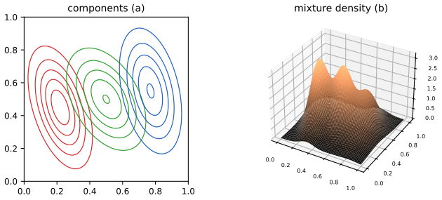
fig_3_11. Download: PDF · SVG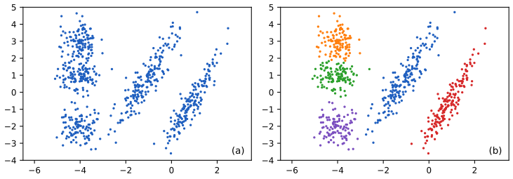
fig_3_12. Download: PDF · SVG3.5.2 Bernoulli mixture models
pp. 98–99 For binary vectors \(\mathbf{y}\in\{0,1\}^D\) the component is a product of independent Bernoullis,
\[ p(\mathbf{y}\given z=k,\boldsymbol\theta)=\prod_{d=1}^D\operatorname{Ber}(y_d\given\mu_{dk})=\prod_{d=1}^D\mu_{dk}^{y_d}(1-\mu_{dk})^{1-y_d}, \tag{3.102} \]with \(\mu_{dk}\) the probability that pixel \(d\) is on in cluster \(k\). Within a cluster the pixels are independent, but marginally (after summing over \(k\)) they are dependent: the mixture captures correlations that a single product of Bernoullis cannot.
Filling the gap 3.14: EM for a mixture of Bernoullis p. 98 (the book defers to Section 8.7.3)
Derivation
Idea. The log likelihood \(\sum_n\log\sum_k\pi_kp(\mathbf{y}_n\given\boldsymbol\theta_k)\) has a sum inside the logarithm. EM maximises it by alternating two steps, each of which is a closed form.
E step. With current parameters \(\boldsymbol\theta^{\mathrm{old}}\), compute the responsibilities (3.99) \(r_{nk}\propto\pi_k\prod_d\mu_{dk}^{y_{nd}}(1-\mu_{dk})^{1-y_{nd}}\) (in the log domain with a log-sum-exp for numerical stability).
M step. Maximise the expected complete-data log likelihood \[Q(\boldsymbol\theta)=\sum_{n,k}r_{nk}\big[\log\pi_k+\sum_d\big(y_{nd}\log\mu_{dk}+(1-y_{nd})\log(1-\mu_{dk})\big)\big]\]. For \(\boldsymbol\pi\) with the constraint \(\sum_k\pi_k=1\), the Lagrangian condition \(\sum_nr_{nk}/\pi_k=\nu\) and normalisation give \(\pi_k=N_k/N\) with \(N_k=\sum_nr_{nk}\). For \(\mu_{dk}\), \(\partial Q/\partial\mu_{dk}=\sum_nr_{nk}\big[\frac{y_{nd}}{\mu_{dk}}-\frac{1-y_{nd}}{1-\mu_{dk}}\big]=0\) gives
\[ \pi_k=\frac{N_k}N,\qquad \mu_{dk}=\frac{\sum_nr_{nk}y_{nd}}{N_k}: \]the responsibility-weighted mean of the data, so \(\boldsymbol\mu_k\) is the average image of the cluster (Figure 3.13).
Monotone. By Jensen's inequality, for any distributions \(q_n(k)\), \[\sum_n\log p(\mathbf{y}_n\given\boldsymbol\theta)\ge\sum_{n,k}q_n(k)\log\frac{p(\mathbf{y}_n,z_n=k\given\boldsymbol\theta)}{q_n(k)}\], with equality when \(q_n(k)=p(z_n=k\given\mathbf{y}_n,\boldsymbol\theta)\). Choosing \(q_n=r_{n\cdot}\) from \(\boldsymbol\theta^{\mathrm{old}}\) makes the bound tight at \(\boldsymbol\theta^{\mathrm{old}}\); maximising it over \(\boldsymbol\theta\) (the M step) cannot decrease the bound, hence cannot decrease the log likelihood. In the run for Figure 3.13 the log likelihood is non-decreasing at every iteration (checked numerically), and the clipping \(\mu_{dk}\in[10^{-3},1-10^{-3}]\) used in the code prevents \(\log0\) for pixels that are never on in a cluster (the maximum likelihood estimate would be exactly 0 there, a degenerate solution; a Beta prior gives the same cure in a principled way). ∎
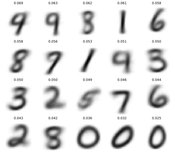
fig_3_13. Download: PDF · SVG3.6 Probabilistic graphical models
p. 99 Section 3.3 showed how a high-dimensional Gaussian \(p(\mathbf{y})\) is built from a marginal \(p(\mathbf{y}_1)\) and a conditional \(p(\mathbf{y}_2\given\mathbf{y}_1)\). The same idea extends to many variables when some of them are conditionally independent of others, and a graph is used to record which.
See also (companion courses): Bayesian and Probabilistic Machine Learning, Section 8.1 (Bayesian networks) and Probability and Statistical Inference, Section 17.4 (probability and DAGs).
3.6.1 Representation
pp. 99–101 A probabilistic graphical model (PGM) is a joint distribution whose graph encodes conditional independence: each node is a random variable, and the absence of an edge is a conditional independence. For a directed acyclic graph (DAG), number the nodes in topological order (parents before children); the model asserts the ordered Markov property: each node is conditionally independent of its other predecessors given its parents,
\[ Y_i\ \perp\ \mathbf{Y}_{\operatorname{pred}(i)\setminus\operatorname{pa}(i)}\ \big|\ \mathbf{Y}_{\operatorname{pa}(i)}, \tag{3.103} \]and, consequently, the joint distribution factorises as
\[ p(Y_{1:N_G})=\prod_{i=1}^{N_G}p\big(Y_i\given\mathbf{Y}_{\operatorname{pa}(i)}\big). \tag{3.104} \]Result 3.9 (ordered Markov property \(\Leftrightarrow\) factorisation; parameter counts) pp. 99–101, (3.103)–(3.106)
(a) For a DAG with topologically ordered nodes, (3.103) holds for all \(i\) if and only if the joint distribution factorises as (3.104). (b) If every node \(i\) is categorical with \(K_i\) states and each conditional table is unrestricted, the model has \(\sum_i(K_i-1)J_i\) free parameters, where \(J_i=\prod_{p\in\operatorname{pa}(i)}K_p\), against \(\prod_iK_i-1\) for an unrestricted joint distribution.
Proof
(a) By the chain rule of probability (3.107), \(p(Y_{1:N})=\prod_ip(Y_i\given Y_{1:i-1})\), and \(Y_{1:i-1}\) is the set of predecessors. If (3.103) holds, then since \(\operatorname{pa}(i)\subseteq\operatorname{pred}(i)\) the conditioning set can be reduced to the parents: \(p(Y_i\given\mathbf{Y}_{\operatorname{pred}(i)})=p(Y_i\given\mathbf{Y}_{\operatorname{pa}(i)})\), which yields (3.104). Conversely, suppose (3.104). Summing the joint over the later nodes \(Y_N,Y_{N-1},\dots,Y_{i+1}\) in turn removes their factors (each conditional sums to one over its own variable and, in topological order, no earlier factor involves a later node), so \(p(Y_{1:i})=\prod_{j\le i}p(Y_j\given\mathbf{Y}_{\operatorname{pa}(j)})\) and dividing by \(p(Y_{1:i-1})\) gives \(p(Y_i\given Y_{1:i-1})=p(Y_i\given\mathbf{Y}_{\operatorname{pa}(i)})\), which is (3.103).
(b) A conditional probability table (CPT) \(\theta_{ijk}=p(Y_i=k\given\mathbf{Y}_{\operatorname{pa}(i)}=j)\) (3.106) has \(J_i\) rows, each a distribution on \(K_i\) states with \(K_i-1\) free entries (the row sums to 1). ∎
Filling the gap 3.15a: the sprinkler factorisation and parameter count p. 100, (3.105)
Derivation
Order the nodes \(C,S,R,W\). The ordered Markov property says: \(S\) has parent \(C\) and no other predecessors, so no reduction; \(R\) has predecessors \(C,S\) and parent \(C\) alone, so \(R\perp S\given C\) (given the cloudy season, whether the sprinkler is on says nothing more about rain); \(W\) has parents \(S,R\) and predecessor \(C\) too, so \(W\perp C\given S,R\). Hence \[p(C,S,R,W)=p(C)\,p(S\given C)\,p(R\given C)\,p(W\given S,R)\] (3.105). The tables have \(1+2+2+4=9\) free parameters (rows: 1, 2, 2, 4 with one free entry each for binary nodes) against \(2^4-1=15\) for an arbitrary joint distribution on four bits: the saving of the conditional independences. The sixteen joint probabilities sum to 1 (confirmed numerically), and \(p(S\given C)p(R\given C)\) is exactly the joint of \(S,R\) given \(C\) (a numerical experiment of the first independence). ∎
Filling the gap 3.15b: Markov chains, parameter tying and parameter counts pp. 101–102, (3.107)–(3.109)
Derivation
For \(T\) variables with \(K\) states, the chain rule gives (3.107) with \(p(y_t\given y_{1:t-1})\) needing \(K^{t-1}(K-1)\) numbers, so a full joint needs \(K^T-1\) in total. The first-order Markov condition \(\mathbf{y}_{t+1:T}\perp\mathbf{y}_{1:t-1}\given y_t\) reduces each factor to \(p(y_t\given y_{t-1})\) (3.108). With a homogeneous transition matrix \(A_{jk}=p(y_t=k\given y_{t-1}=j)\) (rows sum to 1) the whole chain has \(K-1\) parameters for the initial distribution and \(K(K-1)\) for \(\mathbf{A}\), independent of \(T\): this is parameter tying. An order-\(M\) chain (3.109) needs \(K^M(K-1)\) transition parameters, the exponential growth in \(M\) that motivates neural language models. The joint (3.108) sums to one over all \(K^T\) sequences (numerically confirmed for \(K=3\), \(T=4\)): summing out \(y_T\) first leaves a chain of length \(T-1\), and by induction down to \(\sum_{y_1}p(y_1)=1\). ∎
3.6.2 Inference
p. 102 A PGM defines a joint distribution, so any conditional \(p(Y_i\given Y_j=y_j)\) follows from marginalisation and conditioning. For the sprinkler network (Figure 3.14) the prior probability of rain is \(p(R=1)=0.5\); after seeing wet grass it becomes \(p(R=1\given W=1)=0.7079\); after also noticing that the sprinkler is on it falls to \(p(R=1\given W=1,S=1)=0.3204\). This competition between causes of a shared effect is explaining away (Berkson's paradox).
Filling the gap 3.15: the explaining-away calculation by hand p. 102
The book quotes the numbers and refers to code. Here is the arithmetic, from the tables of Figure 3.14: \(p(C=1)=0.5\); \(p(S=1\given C=0,1)=0.5,0.1\); \(p(R=1\given C=0,1)=0.2,0.8\); \(p(W=1\given S,R)=0\), \(0.9\), \(0.9\), \(0.99\) for \((S,R)=(0,0),(1,0),(0,1),(1,1)\).
Derivation
Prior on rain. \(p(R=1)=\tfrac12(0.2)+\tfrac12(0.8)=0.5\).
Marginalising out \(C\). Summing the joint over \(C\) gives \[p(S=s,R=r)=\sum_cp(c)p(s\given c)p(r\given c)\]. For \((s,r)=(0,0)\): \[0.5\cdot0.5\cdot0.8+0.5\cdot0.9\cdot0.2=0.20+0.09=0.29\]; for \((1,0)\): \(0.5\cdot0.5\cdot0.8+0.5\cdot0.1\cdot0.2=0.21\); for \((0,1)\): \[0.5\cdot0.5\cdot0.2+0.5\cdot0.9\cdot0.8=0.05+0.36=0.41\]; for \((1,1)\): \[0.5\cdot0.5\cdot0.2+0.5\cdot0.1\cdot0.8=0.05+0.04=0.09\]. They sum to 1.
Evidence W = 1. Weighting by \(p(W=1\given S,R)\):
\[ p(W=1)=0.29(0)+0.21(0.9)+0.41(0.9)+0.09(0.99)=0.189+0.369+0.0891=0.6471, \] \[ p(R=1,W=1)=0.41(0.9)+0.09(0.99)=0.369+0.0891=0.4581,\qquad p(R=1\given W=1)=\frac{0.4581}{0.6471}=0.7079. \]Evidence W = 1 and S = 1. \[p(S=1,W=1)=0.21(0.9)+0.09(0.99)=0.189+0.0891=0.2781\] and \(p(S=1,R=1,W=1)=0.0891\), so
\[ p(R=1\given W=1,S=1)=\frac{0.0891}{0.2781}=0.3204. \]Why it goes down. Marginally \(S\) and \(R\) are dependent through \(C\) (a cloudy season makes rain likely and the sprinkler unlikely), but given \(C\) they are independent. Conditioning on the common effect \(W\) creates a different, negative dependence: the grass being wet is more likely when either cause is present, so learning that one cause is present makes the other less necessary. In the extreme case \(S=0\) with \(W=1\) forces rain, because \(p(W=1\given S=0,R=0)=0\): then \(p(R=1\given W=1,S=0)=1\). (The numerical values were also confirmed by brute-force enumeration in code, and the demo computes them with editable tables.) ∎
See also (companion course): Section 8.2.1 (three example graphs: tail-to-tail, head-to-tail, head-to-head) and the d-separation demo: the explaining-away structure is the head-to-head case.
3.6.3 Learning
pp. 102–103 If the parameters of the conditional distributions are unknown they can be added to the graph as further random variables and inferred. For \(N\) data points \(\mathbf{y}_n\) generated independently from \(p(\mathbf{y}\given\boldsymbol\theta)\) with \(\boldsymbol\theta\sim p(\boldsymbol\theta)\) (3.110–3.111), the joint is \(p(\mathcal D,\boldsymbol\theta)=p(\boldsymbol\theta)\prod_np(\mathbf{y}_n\given\boldsymbol\theta)\) (3.112–3.113). Plate notation (Figure 3.16) draws one copy of the repeated node inside a box labelled with the repetition count; the Gaussian mixture of Figure 3.17 has the joint \[p(\mathbf{y}_{1:N},\mathbf{z}_{1:N},\boldsymbol\theta)=p(\boldsymbol\pi)\big[\prod_kp(\boldsymbol\mu_k)p(\boldsymbol\Sigma_k)\big]\big[\prod_np(z_n\given\boldsymbol\pi)p(\mathbf{y}_n\given z_n,\boldsymbol\mu_{1:K},\boldsymbol\Sigma_{1:K})\big]\] (3.114).
Filling the gap 3.16: exchangeability p. 102
Derivation
A sequence \(\mathbf{y}_1,\dots,\mathbf{y}_N\) is exchangeable if its joint distribution is invariant under every permutation of the indices. Data that are iid given \(\boldsymbol\theta\) are exchangeable: the marginal joint is \(p(\mathbf{y}_{1:N})=\int p(\boldsymbol\theta)\prod_np(\mathbf{y}_n\given\boldsymbol\theta)\d\boldsymbol\theta\), and the product (hence the integral) does not change when the factors are permuted. They are not independent marginally (observing some \(\mathbf{y}_n\) is informative about \(\boldsymbol\theta\), hence about the others) but exchangeable, which is why the order of the observations does not matter to the posterior, as in the sequential-equals-batch property of gap 3.10. The converse is a theorem of de Finetti (1937; for infinite sequences of binary variables, extended by Hewitt and Savage, 1955): an infinite exchangeable sequence is a mixture of iid sequences, that is, it has the form above for some prior over \(\boldsymbol\theta\). This is the justification for modelling "iid given a parameter" in a Bayesian analysis. ∎
Exercises
All 8 exercises of Chapter 3 (Murphy, 2022, pp. 103–105), restated in my own words, with complete solutions (hidden). Each solution was worked out independently; the computational claims were also confirmed by simulation or numerical integration.
Exercise 3.1 (uncorrelated does not imply independent). Let \(X\sim U(-1,1)\) and \(Y=X^2\). \(Y\) is a function of \(X\), hence dependent on it. Show that \(\rho(X,Y)=0\). (Hint: for \(X\sim U(a,b)\), \(\E X=(a+b)/2\) and \(\mathbb V[X]=(b-a)^2/12\).)
Solution
\(\E X=0\) and \(\E[X^3]=0\) (odd function integrated against the symmetric density \(\tfrac12\) on \([-1,1]\)). Then \[\cov[X,Y]=\E[X\cdot X^2]-\E X\,\E[X^2]=\E[X^3]-0=0\]. The correlation is \(0/\sqrt{\mathbb V[X]\mathbb V[Y]}\), defined because \(\mathbb V[X]=\tfrac13\) and \[\mathbb V[Y]=\E X^4-(\E X^2)^2=\tfrac15-\tfrac19=\tfrac4{45}>0\], and equals 0. The strongest possible dependence (\(Y\) is a deterministic function of \(X\)) thus gives zero correlation: correlation only sees the linear part (gap 3.2: the best linear predictor of \(Y\) from \(X\) is the constant \(\E Y\), since the slope \(\cov/\mathbb V[X]\) is 0). Confirmed by numerical integration.
Exercise 3.2 (correlation lies in \([-1,1]\)). Prove \(-1\le\rho(X,Y)\le1\).
Solution
See Result 3.1(a): with the standardised variables \(U=(X-\E X)/\sigma_X\), \(V=(Y-\E Y)/\sigma_Y\), \(0\le\E[(U\mp V)^2]=2\mp2\rho\), hence \(|\rho|\le1\). (An alternative is the Cauchy–Schwarz inequality \(|\E[UV]|\le\sqrt{\E U^2\,\E V^2}=1\).) The two variances must be positive for \(\rho\) to be defined.
Exercise 3.3 (linearly related variables). If \(Y=aX+b\) with \(a>0\), show \(\rho(X,Y)=1\); if \(a\lt 0\), show \(\rho(X,Y)=-1\).
Solution
\(\E Y=a\E X+b\), so \(Y-\E Y=a(X-\E X)\). Then \(\cov[X,Y]=a\,\mathbb V[X]\) and \(\mathbb V[Y]=a^2\mathbb V[X]\), so \(\rho=\dfrac{a\mathbb V[X]}{\sqrt{\mathbb V[X]\,a^2\mathbb V[X]}}=\dfrac{a}{|a|}=\operatorname{sgn}(a)\) (for \(\mathbb V[X]>0\)). The converse is Result 3.1(b).
Exercise 3.4 (linear combinations). Let \(\mathbf{x}\) have mean \(\mathbf{m}\) and covariance \(\boldsymbol\Sigma\), and let \(\mathbf{A},\mathbf{B}\) be matrices. (a) Find \(\cov[\mathbf{A}\mathbf{x}]\). (b) Show \(\operatorname{tr}(\mathbf{A}\mathbf{B})=\operatorname{tr}(\mathbf{B}\mathbf{A})\). (c) Find \(\E[\mathbf{x}^\T\mathbf{A}\mathbf{x}]\).
Solution
(a) \(\cov[\mathbf{A}\mathbf{x}]=\mathbf{A}\boldsymbol\Sigma\mathbf{A}^\T\) (gap 3.1, (3.5)). (b) For \(\mathbf{A}\) of size \(m\times n\) and \(\mathbf{B}\) of size \(n\times m\), \[\operatorname{tr}(\mathbf{A}\mathbf{B})=\sum_{i=1}^m\sum_{j=1}^nA_{ij}B_{ji}=\sum_{j=1}^n\sum_{i=1}^mB_{ji}A_{ij}=\operatorname{tr}(\mathbf{B}\mathbf{A})\]. (c) A scalar equals its own trace, so \(\mathbf{x}^\T\mathbf{A}\mathbf{x}=\operatorname{tr}(\mathbf{x}^\T\mathbf{A}\mathbf{x})=\operatorname{tr}(\mathbf{A}\mathbf{x}\mathbf{x}^\T)\) by (b) (with the factors \(\mathbf{x}^\T\) and \(\mathbf{A}\mathbf{x}\)). Taking expectations (trace is linear) and using (3.4):
\[ \E[\mathbf{x}^\T\mathbf{A}\mathbf{x}]=\operatorname{tr}\big(\mathbf{A}\,\E[\mathbf{x}\mathbf{x}^\T]\big)=\operatorname{tr}(\mathbf{A}\boldsymbol\Sigma)+\mathbf{m}^\T\mathbf{A}\mathbf{m}. \]Confirmed by simulation (400 000 draws, a random \(4\times4\) \(\mathbf{A}\)). A special case: for \(\mathbf{A}=\mathbf{I}\), \(\E\|\mathbf{x}\|^2=\operatorname{tr}\boldsymbol\Sigma+\|\mathbf{m}\|^2\).
Exercise 3.5 (Gaussian versus jointly Gaussian). Let \(X\sim\mathcal N(0,1)\) and \(Y=WX\) with \(W=\pm1\) each with probability \(\tfrac12\), independent of \(X\). (a) Show \(Y\sim\mathcal N(0,1)\). (b) Show \(\cov[X,Y]=0\); so \(X,Y\) are uncorrelated yet dependent although both are Gaussian. (Hint: iterated expectation.)
Solution
(a) \[\Pr(Y\le y)=\tfrac12\Pr(X\le y)+\tfrac12\Pr(-X\le y)=\Phi(y)\], because \(X\) and \(-X\) have the same distribution. (b) \(\E Y=\E[W]\E[X]=0\) and \[\E[XY]=\E[\E[WX^2\given W]]=\E[W\,\E X^2]=\E[W]=0\], so \(\cov[X,Y]=0-0=0\) (3.115–3.116). Dependence: \(Y^2=X^2\), so \[\cov[X^2,Y^2]=\mathbb V[X^2]=\E X^4-1=2\ne0\]. This does not contradict gap 3.3 because \((X,Y)\) is not jointly Gaussian (\(X+Y\) has an atom at 0 of mass \(\tfrac12\)). A simulation with \(10^6\) draws confirms \(Y\sim\mathcal N(0,1)\) (Kolmogorov–Smirnov), the zero covariance and \(\cov[X^2,Y^2]\approx2\).
Exercise 3.6 (normalising constant of the multivariate Gaussian). Prove \[\int\exp\big(-\tfrac12(\mathbf{x}-\boldsymbol\mu)^\T\boldsymbol\Sigma^{-1}(\mathbf{x}-\boldsymbol\mu)\big)\d\mathbf{x}=(2\pi)^{d/2}|\boldsymbol\Sigma|^{1/2}\]. (Hint: diagonalise \(\boldsymbol\Sigma\), use \(|\boldsymbol\Sigma|=\prod_i\lambda_i\), change variables, and use the univariate constant.)
Solution
This is gap 3.5. Write \(\boldsymbol\Sigma=\mathbf{U}\boldsymbol\Lambda\mathbf{U}^\T\), substitute \(\mathbf{z}=\mathbf{U}^\T(\mathbf{x}-\boldsymbol\mu)\) (orthogonal, Jacobian 1), so the quadratic form becomes \(\sum_iz_i^2/\lambda_i\) and the integral splits into \[\prod_i\int e^{-z_i^2/(2\lambda_i)}\d z_i=\prod_i\sqrt{2\pi\lambda_i}=(2\pi)^{d/2}\big(\prod_i\lambda_i\big)^{1/2}=(2\pi)^{d/2}|\boldsymbol\Sigma|^{1/2}\]. Confirmed by numerical double integration for a \(2\times2\) example.
Exercise 3.7 (sensor fusion with known variances in one dimension). Two sensors have known variances \(v_1\ne v_2\) and share an unknown mean \(\mu\). Sensor 1 gives \(n_1\) readings \(y^{(1)}_i\sim\mathcal N(\mu,v_1)\), sensor 2 gives \(n_2\) readings \(y^{(2)}_i\sim\mathcal N(\mu,v_2)\). With a non-informative prior (a Gaussian of precision 0), find the posterior \(p(\mu\given\mathcal D)\): mean and variance explicitly.
Solution
The log posterior is, up to a constant, \[-\tfrac12\sum_i(y^{(1)}_i-\mu)^2/v_1-\tfrac12\sum_i(y^{(2)}_i-\mu)^2/v_2\], a quadratic in \(\mu\) with coefficient of \(\mu^2\) equal to \(-\tfrac12(n_1/v_1+n_2/v_2)\) and linear coefficient \(\sum_iy^{(1)}_i/v_1+\sum_iy^{(2)}_i/v_2\). Completing the square (gap 3.9):
\[ \mu\given\mathcal D\sim\mathcal N(m,s^2),\qquad s^2=\Big(\frac{n_1}{v_1}+\frac{n_2}{v_2}\Big)^{-1},\qquad m=s^2\Big(\frac{n_1\bar y^{(1)}}{v_1}+\frac{n_2\bar y^{(2)}}{v_2}\Big)=\frac{n_1v_2\bar y^{(1)}+n_2v_1\bar y^{(2)}}{n_1v_2+n_2v_1}. \]Each reading counts with weight \(1/v\), so one precise reading can outweigh several imprecise ones; the posterior variance \(s^2\) is smaller than either sensor's alone. A numerical grid integration of the posterior for simulated data agrees with these values to \(10^{-6}\).
Exercise 3.8 (Student distribution as a Gaussian scale mixture). Show that\[ p(x\given\mu,a,b)=\int_0^\infty\mathcal N(x\given\mu,\alpha^{-1})\operatorname{Ga}(\alpha\given a,b)\d\alpha \tag{3.118} \]is a Student distribution, where \(\operatorname{Ga}(\alpha\given a,b)=b^a\alpha^{a-1}e^{-b\alpha}/\Gamma(a)\) (rate \(b\)).
Solution
Insert the two densities, \(\mathcal N(x\given\mu,\alpha^{-1})=(\alpha/2\pi)^{1/2}e^{-\alpha(x-\mu)^2/2}\):
\[ p(x)=\frac{b^a}{\Gamma(a)\sqrt{2\pi}}\int_0^\infty\alpha^{a-1/2}\exp\Big[-\alpha\Big(b+\frac{(x-\mu)^2}2\Big)\Big]\d\alpha=\frac{b^a}{\Gamma(a)\sqrt{2\pi}}\,\Gamma\big(a+\tfrac12\big)\Big(b+\frac{(x-\mu)^2}2\Big)^{-a-1/2}, \]using \(\int_0^\infty\alpha^{s-1}e^{-c\alpha}\d\alpha=\Gamma(s)c^{-s}\) with \(s=a+\tfrac12\). Factor \(b\) out of the bracket:
\[ p(x)=\frac{\Gamma(a+\tfrac12)}{\Gamma(a)\sqrt{2\pi b}}\Big(1+\frac{(x-\mu)^2}{2b}\Big)^{-(a+1/2)}. \]The Student density with \(\nu\) degrees of freedom, location \(\mu\) and scale \(\sigma^2\) is \(\frac{\Gamma((\nu+1)/2)}{\Gamma(\nu/2)\sqrt{\nu\pi\sigma^2}}\big(1+\frac{(x-\mu)^2}{\nu\sigma^2}\big)^{-(\nu+1)/2}\). Matching exponents, \(\nu=2a\); matching the bracket, \(\nu\sigma^2=2b\), i.e. \(\sigma^2=b/a\); and then \(\nu\pi\sigma^2=2\pi b\), so the constants agree. Hence \(x\sim\mathcal T_{2a}(\mu,b/a)\): an infinite mixture of Gaussians with gamma-distributed precision, with heavier tails than a Gaussian because small precisions (large variances) have positive probability. As \(a\to\infty\) with \(b=a\) the precision concentrates at 1 and the mixture tends to \(\mathcal N(\mu,1)\). Verified by numerical integration at a test point.
Demonstrations
| Demonstration | What you can see | Sections and results |
|---|---|---|
| The bivariate Gaussian | Samples, the 1, 2 and 3 standard deviation ellipses, eigenvector axes, the marginal density of \(y_1\), and the conditional density given an observed \(y_2\) (click the plot or use the slider); the sample mean and covariance of the iris sepals. Presets: 1 \(\rho=0.8\); 2 uncorrelated; 3 \(\rho=0.97\); 4 unequal scales; 5 iris. | 3.2.1, 3.2.2, 3.2.3, 3.2.4; gap 3.2 |
| Bayes rule for Gaussians and sensor fusion | The prior, the data and the posterior of an unknown 2d location after N noisy points (N from 1 to 50, prior width adjustable), and the fusion of two sensors whose noise in each direction you set. Presets: 1 N = 1; 2 N = 10; 3 weak prior; 4, 5, 6 Figures 3.10a to c. | 3.3.1, 3.3.4, 3.3.5; Result 3.6, gap 3.12 |
| The water sprinkler network | Choose evidence for any of the four nodes and read off the exact posterior of the others; edit the nine table entries. Presets: 1 prior; 2 wet grass; 3 explaining away; 4 sprinkler off; 5 conditional independence; 6 leaky grass. | 3.6.1, 3.6.2; Result 3.9, gap 3.15 |
| Correlation and Simpson's paradox | The iris sepal data with any subset of species: correlations, slopes, one line per group and a line for the union. Presets: 1 pooled; 2 one line per species; 3 setosa; 4 versicolor and virginica; 5 setosa and versicolor. | 3.1.2, 3.1.5; Result 3.3 |
The Python code that produces every figure of this page is code/ch03_probability_multivariate.py (see the code index). Companion demonstrations: conjugate priors, mixture densities, K-means and EM, d-separation.
References
- Murphy, K. P. (2022). Probabilistic Machine Learning: An Introduction. MIT Press, Cambridge, MA. Chapter 3, pp. 77–105. probml.github.io/pml-book/book1.html.
- Bishop, C. M. (2006). Pattern Recognition and Machine Learning. Springer, New York.
- de Finetti, B. (1937). La prévision: ses lois logiques, ses sources subjectives. Annales de l'Institut Henri Poincaré, 7, 1–68.
- Dempster, A. P., Laird, N. M. and Rubin, D. B. (1977). Maximum likelihood from incomplete data via the EM algorithm. Journal of the Royal Statistical Society, Series B, 39(1), 1–38.
- Fisher, R. A. (1936). The use of multiple measurements in taxonomic problems. Annals of Eugenics, 7(2), 179–188.
- Hewitt, E. and Savage, L. J. (1955). Symmetric measures on Cartesian products. Transactions of the American Mathematical Society, 80, 470–501.
- Jaynes, E. T. (1957). Information theory and statistical mechanics. Physical Review, 106(4), 620–630.
- Koller, D. and Friedman, N. (2009). Probabilistic Graphical Models: Principles and Techniques. MIT Press, Cambridge, MA.
- LeCun, Y., Bottou, L., Bengio, Y. and Haffner, P. (1998). Gradient-based learning applied to document recognition. Proceedings of the IEEE, 86(11), 2278–2324.
- Pearl, J. (1988). Probabilistic Reasoning in Intelligent Systems. Morgan Kaufmann, San Francisco.
- Simpson, E. H. (1951). The interpretation of interaction in contingency tables. Journal of the Royal Statistical Society, Series B, 13(2), 238–241.
- Wasserman, L. (2004). All of Statistics: A Concise Course in Statistical Inference. Springer, New York.
The numerical statements in the text (covariance identities, the bound on the correlation, the normalising constant, the three forms of the conditional mean, Bayes rule for Gaussians and its equivalence with conditioning the joint, sequential and batch updating, sensor fusion, the cumulants of exponential families, maximum entropy, mixture moments, monotone EM, the sprinkler probabilities and the Student mixture) were confirmed numerically.