Interpretability
Chapter 33 is a framework, not an algorithm: to ask whether a model can be understood one must say who the user is (the context), what they are trying to do (the end-task), what is shown to them (the method), how success is measured (the metrics) and what the explanation must be like (the properties). These notes follow the book and then do what the chapter cannot do in prose: they compute its examples, state its properties as formulas, prove the facts it asserts about faithfulness, stability, sanity checks, insertion tests and the design of user studies, and let you play with three of them.
Ch. 1 Introduction Ch. 2 Probability Ch. 3 Statistics Ch. 4 Graphical models Ch. 5 Information theory Ch. 6 Optimisation Ch. 7 Inference algorithms Ch. 8 Gaussian filtering Ch. 9 Message passing Ch. 10 Variational inference Ch. 11 Monte Carlo Ch. 12 MCMC Ch. 13 Sequential Monte Carlo Ch. 14 Predictive models Ch. 15 GLMs Ch. 16 Deep networks Ch. 17 Bayesian neural networks Ch. 18 Gaussian processes Ch. 19 Beyond iid Ch. 20 Generative models Ch. 21 VAEs Ch. 22 Autoregressive models Ch. 23 Normalizing flows Ch. 24 Energy-based models Ch. 25 Diffusion models Ch. 26 GANs Ch. 27 Discovery methods Ch. 28 Latent factor models Ch. 29 State-space models Ch. 30 Graph learning Ch. 31 Nonparametric Bayes Ch. 32 Representation learning Ch. 33 Interpretability Ch. 34 Decision making Ch. 35 Reinforcement learning Ch. 36 Causality
How to read these notes
They follow the book. Sections carry the book's numbers. The chapter has two numbered equations, (33.1) and (33.2), both in the lemonade-stand example, and they keep their numbers. Page numbers in the grey tags are the book's.
Filling the gaps. Orange Filling the gap boxes give the full argument for what the chapter states in words: what the two lemonade explanations compute and why one of them changes with the units, what correlated features do to a sparse model, how a surrogate's fidelity bounds its accuracy, what a local linear explanation converges to as the neighbourhood shrinks, when an explanation is stable, what Shapley values are, why a randomisation test and a shift test are informative, when insertion curves are trustworthy, why matching raises power, why randomisation removes confounding, and why Holm's procedure controls the family-wise error. Proofs start hidden.
Figures. The book's one computed figure (33.2) is reproduced. Figures 33.1 (a diagram), 33.3 to 33.6 (photographs and saliency maps of image classifiers) are not: they need pre-trained networks and image data. Seven figures of my own, computed on small stand-ins, replace them where a computation can make the same point (named x33.1 to x33.7).
A caution from the book. The authors add a footnote that later theory shows several popular attribution methods (integrated gradients, SHAP) can provably do no better than chance at explaining behaviour, and that some researchers doubt the field's foundations. The notes keep that in view: much of what follows is about how to tell when an explanation is not telling you anything.
Main reference
K. P. Murphy, Probabilistic Machine Learning: Advanced Topics, MIT Press (2023; December 2025 draft), Chapter 33 (written by Been Kim and Finale Doshi-Velez), pages 1073–1102, and the supplement, Chapter 33 (title page only). Book web page: probml.github.io/pml-book/book2.html. The text here is my own wording; equations are restated.
Companion courses
- Probabilistic Machine Learning: An Introduction: Chapter 11 linear regression (ridge, lasso, collinearity), Chapter 10 logistic regression, Chapter 18 trees, forests and boosting, Chapter 16 exemplar-based methods (k-nearest neighbours), Chapter 5 decision theory.
- All of Statistics: Chapter 10 hypothesis testing (the t-test, power, multiple testing) and Chapter 16 causal inference (randomisation, potential outcomes); An Introduction to Statistical Learning: Chapter 13 multiple testing.
- Elements of Statistical Learning: Chapter 3 linear regression (shrinkage and selection), Chapter 9 additive models and trees; Foundations of Deep Learning: Chapter 8 backpropagation (input gradients).
33.1 Introduction
p. 1073 A model can score well on the metric it was trained for and still be harmful: the metric may be too narrow (a car that stays in its lane is not thereby safe), the data may reward shortcuts, the quantity may be hard to estimate under distribution shift (Chapter 19), or the norm itself (fairness) may not be formalisable. Interpretability lets a human inspect a model, which can expose such problems, let the person combine what they know with what the model computes, and teach us why a model works.
33.1.1 The role of interpretability: unknowns and under-specifications
pp. 1074–1075 Where the goal can be written down (differential privacy, a chosen fairness metric) or well-calibrated uncertainty is available (Chapters 3, 17, 18), no inspection is needed. Interpretability earns its place when the goal cannot be fully specified. The chapter gives four typical uses, each with a different user and time budget:
- Blindspot discovery: inspecting a credit model reveals it leans on mortgage payments, which flags both a poor fit to a younger population and a historical bias in home ownership.
- Novel insight: clusters of surgeries turn out to share a hospital wing, a feature that was not in the data.
- Human and machine teaming: a treatment recommender reveals that it was constrained by a comorbid insomnia the patient no longer has, so it can be re-run without that constraint.
- Individual recourse: a loan applicant who knows which features were used can argue that an error was made (sometimes a legal requirement).
What these share is that the human must add something to the model. What differs is the scope (global patterns for a scientist, one decision for a clinician) and the time available. Hence the chapter's central claim: the best form of explanation depends on the context, and interpretability is a means to an end.
33.1.2 Terminology and framework
pp. 1075–1078 To interpret is to explain in understandable terms, and understanding is an alignment between what the model is doing and what the user believes it is doing. The vocabulary has five parts, two human and three technical:
| Term | Question it answers | Example |
|---|---|---|
| context | Who is the user, with what information and what limits on time and attention? | a clinician with two minutes |
| end-task | What is the user ultimately trying to achieve? | choose between treatments |
| method | What is shown? The model itself (inherently interpretable) or an explanation, a partial view of it. | a small rule list; a list of important features |
| metrics | How is the method judged? By the user's downstream performance on the end-task. | treatment decisions that agree with an expert panel |
| properties | What must the explanation be like (faithful, compact, stable, ...)? | only features that can be changed |
The properties are the glue: the context and end-task say which are needed, the metrics say how to measure the downstream effect, and the method must supply them (Figure 33.1 in the book, a diagram, shows these relations). Two models that fit the data equally well have different explanations under different methods, and the book's lemonade stand makes this concrete.
Setup: the lemonade stand pp. 1077–1078
Inputs: the day's temperature \(T\) (degrees Fahrenheit) and the cleanliness \(c\in[0,1]\) of the sidewalk. Output: whether the day was profitable. Two models fit the data about equally well:
\[ p(\text{profit}) = 0.9\cdot\ind[T>75] + 0.1\,c \qquad\text{(Model 1)}\tag{33.1} \] \[ p(\text{profit}) = \sigma\!\Big(0.9\,\frac{T-75}{\max T} + 0.1\,(c-0.5)\Big)\qquad\text{(Model 2)}\tag{33.2} \]with \(\sigma\) the logistic function. Both are inherently interpretable and both rely mostly on temperature. Treat them as black boxes and ask for the most important features in two ways. Flip explanation: for each training day set one feature to its minimum and to its maximum; a feature's importance is the share of days whose prediction changes. Derivative explanation: a feature's importance is the sum over training days of the absolute partial derivative of the output.
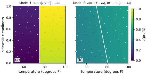
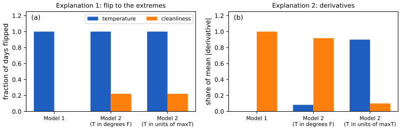
On the 400 days of the design above the flip method names temperature for both models (it flips all 100 percent of the predictions, against 0 percent for cleanliness in Model 1 and 22 percent in Model 2). The derivative method names cleanliness for Model 1, because the step has slope zero at every training day, and, as the next box shows, also for Model 2 when the temperature is in degrees Fahrenheit, though not when it is measured in units of \(\max T\). The two explanations have different properties: the first is faithful about which features change the prediction, the second about local curvature. For deciding whether to trust the model the first is the one that matters, which is the chapter's point: pick the method by the property the end-task needs.
Filling the gap 33.1: both lemonade explanations in closed form, and why the derivative ranking depends on the units pp. 1077–1078
Derivation
Setting. Predicted class \(\hat y=\ind[p>1/2]\). The training temperatures lie in \([T_{\min},T_{\max}]\subset(50,100)\) and straddle 75, the cleanliness values in \([c_{\min},c_{\max}]\approx[0,1]\).
Flip, Model 1. If \(T>75\) then \(p\in[0.9,1]\), otherwise \(p\in[0,0.1]\). Since \(0.1c\in[0,0.1]\) changing \(c\) moves \(p\) inside the same half and never across \(1/2\): the importance of \(c\) is 0. Setting \(T\) to \(T_{\min}<75<T_{\max}\) flips the class of every day (days above 75 flip when set to \(T_{\min}\), days below when set to \(T_{\max}\)): the importance of \(T\) is 1.
Flip, Model 2. The class is \(\ind[a>0]\) with \(a=s(T)+0.1(c-0.5)\) and \(s(T)=0.9(T-75)/\max T\). With \(\max T=100\), \(s(T_{\min})\approx-0.225\) and \(s(T_{\max})\approx+0.224\), larger in size than the cleanliness effect \(|0.1(c-0.5)|\le0.05\), so the two temperature extremes give the two classes and every day flips: importance 1. Because \(a\) is increasing in \(c\), a day's class is that of \(a(T,c_{\min})\) or of \(a(T,c_{\max})\); it flips for one of them exactly when these two have different signs, that is when \[ -0.1(c_{\max}-0.5)<s(T)<-0.1(c_{\min}-0.5)\ \Longleftrightarrow\ |s(T)|\lesssim0.05\ \Longleftrightarrow\ |T-75|\lesssim\frac{0.05\max T}{0.9}=5.56. \] For temperatures spread evenly over 50 degrees this is a fraction \(11.1/50=0.222\) of the days; the design gives 0.22. Cleanliness matters only for days close to the boundary.
Derivatives, Model 1. For \(T\ne75\), \(\partial p/\partial T=0\) and \(\partial p/\partial c=0.1\): mean absolute derivatives 0 and 0.1. A step is differentiable away from 75, and no training day sits at 75.
Derivatives, Model 2. By the chain rule with \(\sigma'(a)=p(1-p)\), \[ \frac{\partial p}{\partial T}=\frac{0.9}{\max T}\,p(1-p),\qquad \frac{\partial p}{\partial c}=0.1\,p(1-p). \] The ratio is the same on every day: \(|\partial_c p|/|\partial_T p|=0.1\max T/0.9=\max T/9\), which is 11.1 for \(\max T=100\). With the temperature in degrees Fahrenheit, as the text says, the cleanliness derivative is eleven times larger (mean absolute values 0.0022 and 0.0249 on the design). The claim that temperature wins holds only if the derivative is taken with respect to the rescaled temperature \(u=T/\max T\) that appears inside (33.2): then \(\partial p/\partial u=0.9\,p(1-p)\) and the ratio is 9 in favour of temperature (0.224 against 0.025). In general, with the temperature measured in units of \(u_0\) degrees, \(\partial p/\partial(T/u_0)=u_0\,\partial p/\partial T\) and the ratio of temperature to cleanliness importance is \(9u_0/\max T\); the two are equal at \(u_0=\max T/9\approx11.1\) degrees. A ranking that reverses when one changes the unit of a feature is a property of the unit.
A smoothed step. Replace the step by \(0.9\,\sigma((T-75)/w)\). Its derivative \(\frac{0.9}{w}\sigma'((T-75)/w)\) is a bump of total area 0.9 (substitute \(v=(T-75)/w\), \(\int\sigma'=1\)). If the training temperatures have density \(\rho(T)\), then \[ \E\Big|\frac{\partial p}{\partial T}\Big|=\int\frac{0.9}{w}\sigma'\!\Big(\frac{T-75}{w}\Big)\rho(T)\,\d T\ \longrightarrow\ 0.9\,\rho(75)\quad(w\to0), \] and equals \(0.9/50=0.018\) per degree whenever the bump lies inside a uniform \([50,100]\). So the mean absolute derivative of any steepness is the jump times the density at the jump, independent of \(w\), and the exact step's value 0 is an artefact of evaluating a measure-zero set of days. On the design the values for \(w=1,2,5\) are 0.0175, 0.0178 and 0.0178. In degrees this is still below cleanliness (0.1), in units of \(\max T\) it is 1.78, far above.
33.2 Methods for interpretable machine learning
p. 1079 The section is a snapshot of a fast-changing field. The organising question is how much of the model the user sees: all of it (the model is its own explanation), examples that stand in for it, or a partial view computed from a trained model.
33.2.1 Inherently interpretable models: the model is its explanation
pp. 1079–1081 A model is inherently interpretable if a person can inspect all of it, with reasonable effort, and understand how inputs become outputs, with no extra process or proxy; note that this depends on the end-task (a rule list is enough when there is no time pressure). Two families:
- Compact or sparse feature-based models: sparse regressions, checklists and super-sparse integer models, small hidden Markov models (Section 29.2), generalized linear models (Chapter 15), small latent-variable models, topic models, generalized additive models and monotone models.
- Logic-based models: decision trees, decision lists, tables and sets, logic programs. They represent non-linear relations easily but approximate a smooth trend by a staircase.
Sparsity has a drawback the book mentions in one sentence: if a model keeps one of several correlated features it is hard to see which signal drives the prediction, and correlated features may receive opposite signs that cancel. The following box quantifies this.
Filling the gap 33.2: correlated features make weights unstable; sparsity picks one of them p. 1079
Derivation
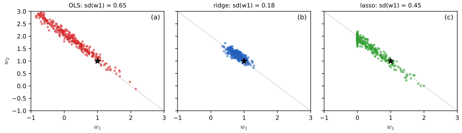
Variance of the weights. Let \(y=w_1x_1+w_2x_2+\varepsilon\), \(\varepsilon\sim\N(0,\sigma^2)\), with the two features of unit variance and correlation \(\rho\), covariance \(\Sigma=\begin{pmatrix}1&\rho\\\rho&1\end{pmatrix}\). Given the design matrix \(X\) (\(n\) rows) the least-squares estimate has covariance \(\sigma^2(X^\T X)^{-1}\) (it is linear in \(y\), and the noise has covariance \(\sigma^2I\)), and \(X^\T X\approx n\Sigma\). With \(\Sigma^{-1}=\frac1{1-\rho^2}\begin{pmatrix}1&-\rho\\-\rho&1\end{pmatrix}\), \[ \var(\hat w_1)\approx\frac{\sigma^2}{n(1-\rho^2)},\qquad \cov(\hat w_1,\hat w_2)\approx\frac{-\rho\,\sigma^2}{n(1-\rho^2)},\qquad \operatorname{corr}(\hat w_1,\hat w_2)\approx-\rho. \] (For Gaussian features \(\E(X^\T X)^{-1}=\Sigma^{-1}/(n-3)\) exactly, so \(n\) becomes \(n-3\).) The variance is inflated by the factor \(1/(1-\rho^2)\) relative to uncorrelated features: 25 for \(\rho=0.98\). The two weights move together in opposite directions: along the line \(\hat w_1+\hat w_2=\) const. Indeed \[ \var(\hat w_1+\hat w_2)\approx\frac{2\sigma^2}{n(1+\rho)},\qquad \var(\hat w_1-\hat w_2)\approx\frac{2\sigma^2}{n(1-\rho)}, \] so the data identify the sum, which is what the prediction uses, and almost nothing about how it is split: the difference is \((1+\rho)/(1-\rho)=99\) times more variable at \(\rho=0.98\). A single fitted model can therefore show \(\hat w=(0.16,1.95)\) while the truth is \((1,1)\), or even weights of opposite signs; reading signs and sizes off such weights as an explanation is unreliable.
Ridge splits, lasso picks. Take two identical features \(x_1=x_2=x\). The squared error depends on \((w_1,w_2)\) only through \(s=w_1+w_2\). For ridge (penalty \(\lambda(w_1^2+w_2^2)\)) at fixed \(s\), \(w_1^2+w_2^2\ge s^2/2\) with equality iff \(w_1=w_2\) (Cauchy–Schwarz), so the minimiser splits the weight equally. For the lasso (penalty \(\lambda(|w_1|+|w_2|)\)) at fixed \(s\), \(|w_1|+|w_2|\ge|s|\) with equality iff \(w_1w_2\ge0\), so every split with both weights of the same sign has the same objective: the solution is not unique, and a solver or a resample decides which feature is kept. With correlation \(\rho<1\) but close to 1 the tie is broken by noise, and a bootstrap shows the lasso keeping \(x_1\) in some resamples and \(x_2\) in others (figure x33.6: one of the two weights is exactly zero in about 37 percent of the resamples), while the ridge weights have standard deviation 0.18 against 0.65 for least squares.
The book names three decisions when using an inherently interpretable model. (i) Model class: since the model is the explanation, choosing the class is choosing the form of explanation, and a model that grows too large to inspect stops being interpretable. (ii) Optimisation: sparse, compact and logic-based models involve discrete parameters and need dedicated methods (programs, relaxation and rounding, search), or distillation (mimicking): fit a complex model and train a simple one to reproduce its outputs; see gap 33.3. (iii) Uninterpretable inputs: pixels or spectrogram amplitudes have no meaning to a person, so one can add a concept layer that maps the raw input to human concepts and then fit an interpretable model on those; the mapping must really implement the concept the user has in mind.
Inherently interpretable models do not need to be checked for faithfulness, give confidence when nothing is found wrong, and are the first thing to try in high-stakes settings. Against that, they need specialised optimisation, may lose accuracy on images, waveforms and text, can invite rationalisation of a poor fit, face resistance when replacing a legacy system, and do not protect against distribution shift. The question of an accuracy trade-off is taken up in Section 33.5.
33.2.2 Semi-inherently interpretable models: example-based methods
p. 1081 An example-based model predicts from similar training instances: k-nearest neighbours is the best known (PML Chapter 16); extensions choose prototypes or exemplars, generate them, learn the similarity through an embedding, or compare parts. Like logic-based models they draw non-linear boundaries. Each single decision is inspectable, since one can show the labelled instances behind it, and for a k-nearest-neighbour vote with \(k\) odd the shown neighbours are the computation, so the explanation is exact. The difficulty is the notion of similarity: the user cannot see which features made two instances close, and the global boundary is hard to convey with examples. This is why the chapter calls the class only semi-inherently interpretable.
33.2.3 Post-hoc or joint training: the explanation gives a partial view of the model
p. 1081 When the model is not inherently interpretable (a large network, a legacy system, a system of models) the explanation is a partial view: an approximation or an incomplete summary. The decisions split into what the explanation consists of and how it is computed.
33.2.3.1 What does the explanation consist of?
pp. 1082–1083 Form. The model class and the explanation are now different objects (a deep network explained by a decision tree). The form can be a list of important input features or concepts; a simpler model approximating the complex one (a local linear approximation, a rule set); prototypical or influential examples; or a contrast against an alternative (counterfactual). Which form helps depends on the task: a contrast between treatments A and B helps choose between A and B, not between A and C. Literature on how people explain in the target setting (for example how nurses and firefighters explain fast decisions) can guide the choice.
Scope: local or global. A local explanation concerns one decision: saliency or attribution maps (derivatives of the output with respect to the input, or perturbation-based variants), a locally fitted simple model such as LIME, influential training points, or nearby inputs with a different prediction (recourse). Its risk is overgeneralisation: the user may apply it to a wider region than it describes, or build a wrong mental model from a few of them. A global explanation concerns the whole model or a collection of inputs: a simple approximating model, concepts that matter across many inputs, or representative examples, perhaps ones near decision boundaries. It is still a partial view; to be accessible it must omit things.
The book gives a rule of thumb that organises the rest of the section: decide first what properties the context needs (Section 33.3), since different forms differ in expressiveness (a feature list or a local linear fit shows no interaction; a local tree does) and the same form behaves differently on different models (a gradient-based explanation is faithful for a smooth model and not for one with spiky contours).
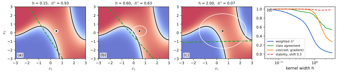
The local linear surrogate is the clearest example to compute, so the next two boxes do. Let \(f\) be the model output, \(x_0\) the input to explain, and fit \(g(x)=a+b^\T(x-x_0)\) to \(f\) with Gaussian locality weights of width \(h\); this is the infinite-sample limit of LIME with a Gaussian kernel and a perturbation distribution wide enough that the kernel does the localising.
Filling the gap 33.4: the local linear explanation is the gradient of the Gaussian-smoothed model pp. 1082–1083
Derivation
Closed form. Let \(\pi_h\) be the density of \(u\sim\N(0,h^2I_d)\) and minimise \(J(a,b)=\E_{\pi_h}\big[(f(x_0+u)-a-b^\T u)^2\big]\) (weighted least squares with weights \(\pi_h\)). Setting the derivatives to zero, \[ \partial_a J=0:\ a=\E f(x_0+u)-b^\T\E u=\E f(x_0+u),\qquad \partial_bJ=0:\ \E[u\,(f(x_0+u)-a-b^\T u)]=0, \] and \(\E[uu^\T]=h^2I\), \(\E[u]=0\) give \[ b=\frac1{h^2}\,\E_{\pi_h}\big[u\,f(x_0+u)\big]. \]
Stein's identity. For \(u\sim\N(0,h^2I)\) and differentiable \(f\) with enough integrability, \(\E[u\,f(x_0+u)]=h^2\E[\nabla f(x_0+u)]\) (integrate by parts using \(\nabla\pi_h(u)=-(u/h^2)\pi_h(u)\); boundary terms vanish). Hence \[ \boxed{\,b=\E_{\pi_h}\big[\nabla f(x_0+u)\big]=\nabla\,(f*\pi_h)(x_0)\,}\qquad a=(f*\pi_h)(x_0), \] the value and gradient at \(x_0\) of the Gaussian smoothing of \(f\) (the idea behind averaging gradients over noisy copies of the input). It also shows the explanation exists for a step function, where the pointwise gradient is useless: for \(f=\ind[x>0]\) in one dimension, \(b=\pi_h(x_0)\), the Gaussian density at \(x_0\).
Small \(h\). The heat-kernel expansion \(f*\pi_h=f+\frac{h^2}{2}\Delta f+O(h^4)\) (Taylor expand \(f(x_0+u)\) to fourth order and use \(\E u_i^2=h^2\), \(\E u_i^4=3h^4\), odd moments zero) gives \[ b=\nabla f(x_0)+\frac{h^2}{2}\nabla(\Delta f)(x_0)+O(h^4). \] So \(b\to\nabla f(x_0)\) as \(h\to0\), with a bias of order \(h^2\) proportional to the third derivatives. In one dimension, \(b=f'+\frac{h^2}2f'''\): for \(f(x)=x^3\) at 0, \(b=3h^2\) while \(f'(0)=0\) (practice problem 33.2). Numerically, for the black box of the demonstration at \(x_0=(0.5,0.2)\) and \(h=0.1\), the departure of \(b\) from the gradient is \((0.0048,0.0034)\) against the predicted \(\frac{h^2}2\nabla\Delta f=(0.0053,0.0035)\).
Fidelity. Write \(f(x_0+u)=f_0+g^\T u+\frac12u^\T Hu+O(|u|^3)\) with \(g=\nabla f(x_0)\), \(H=\nabla^2f(x_0)\). The linear part explains the variance \(h^2|g|^2\) of \(f\) under \(\pi_h\); the quadratic part, after removing its mean, has variance \(\frac14\operatorname{var}(u^\T Hu)=\frac{h^4}{2}\|H\|_F^2\) (for \(u\sim\N(0,h^2I)\) and symmetric \(H\), \(\operatorname{var}(u^\T Hu)=2h^4\operatorname{tr}H^2\)); odd moments make the cross terms vanish. The weighted \(R^2\) is therefore \[ R^2\approx\frac{h^2|g|^2}{h^2|g|^2+\frac{h^4}{2}\|H\|_F^2}\approx1-\frac{h^2\|H\|_F^2}{2|g|^2}\quad(h\to0), \] and the root-mean-square residual is of order \(h^2\|H\|_F\): halving the neighbourhood divides the error by four (ratio 3.8 on the demonstration black box). The price of fidelity is locality: the explanation is faithful only inside a ball of radius about \(h\). As \(h\) grows, \(R^2\) falls (0.97, 0.83, 0.63, 0.28, 0.07 for \(h=0.1,0.3,0.6,1,2\) at \(x_0=(0.5,0.2)\)) and the coefficients leave the gradient: they become the slope of a global Gaussian-weighted linear fit, which for a bounded \(f\) is small because \(\E\nabla f\) averages signs.
Filling the gap 33.5: when is a local explanation stable? pp. 1083, 1087
Derivation
Definition. Write \(E(x)\in\R^d\) for the explanation at \(x\) (the gradient, or the surrogate coefficients). Say it is stable with constant \(L\) if \(\|E(x)-E(x')\|\le L\|x-x'\|\) for all \(x,x'\) (similar inputs, similar explanations).
Gradient explanation. If \(f\) is twice continuously differentiable, \(\nabla f(x)-\nabla f(x')=\int_0^1\nabla^2f(x'+t(x-x'))(x-x')\,\d t\), so the constant is \(L_g=\sup_x\|\nabla^2f(x)\|_{\mathrm{op}}\): the largest curvature. For \(f=\sigma(kx)\) in one dimension, \(f''=k^2\sigma'(kx)(1-2\sigma(kx))\) with extreme value \(k^2/(6\sqrt3)\) (maximise \(\sigma'(1-2\sigma)\): at \(\sigma=\frac12\pm\frac1{2\sqrt3}\) it equals \(\pm\frac1{6\sqrt3}\)). Doubling the steepness quadruples the instability, and for a step (\(k\to\infty\)) there is no stable gradient explanation at all. This is the book's remark that a stable explanation may be impossible when the model has high curvature and the explanation is not expressive.
Smoothed explanation. Since \(b_h=\nabla(f*\pi_h)\) (gap 33.4), \(\nabla b_h=(\nabla^2f)*\pi_h\) when \(f\) is smooth, hence \(L_{b_h}\le L_g\): smoothing never worsens stability. For a bounded model with no smoothness at all, \(\nabla^2(f*\pi_h)=f*\nabla^2\pi_h\), \(\nabla^2\pi_h(u)=\pi_h(u)(uu^\T/h^4-I/h^2)\), and \(\int\nabla^2\pi_h=0\) lets one subtract a constant from \(f\); for a probability \(f\in[0,1]\) subtract \(1/2\): \[ L_{b_h}\le\sup|f-\tfrac12|\cdot\E\big\|uu^\T/h^4-I/h^2\big\|_{\mathrm{op}}\le\frac12\cdot\frac{d+1}{h^2}. \] So a wide kernel gives a Lipschitz explanation of any classifier, even of a step (for \(f=\ind[x>0]\) in one dimension \(b_h=\pi_h\), whose derivative is at most \(1/(h^2\sqrt{2\pi e})\), below the bound \(1/h^2\)), with a constant that grows like \(1/h^2\) as the neighbourhood shrinks. Stability is bought with width, fidelity with narrowness: a trade-off the demonstration lets you see (the stability cosine stays near 1 for large \(h\) while \(R^2\) collapses).
33.2.3.2 How the explanation is computed
pp. 1083–1084 The same form can be computed in many ways, with different properties. For "the most important features" the book lists three definitions of importance: a perturbation definition (the smallest image region that, when changed, changes the prediction, which needs choices about how to perturb: stay within the training distribution? preserve pixel correlations?), a sensitivity definition (largest gradients, again with many computational choices), and a coalition definition (how often a feature belongs to a winning coalition, a Shapley or Banzhaf score). For examples one must decide what similar means (cosine similarity of activations, an \(L_2\) ball); for counterfactuals one can use distances, causal models or SAT formulations. The lemonade stand showed how much the choice matters.
The coalition definition has a precise form worth stating.
Filling the gap 33.6: Shapley values, efficiency, the linear model, and interactions p. 1084
Derivation
Definition. For an input \(x\) with \(d\) features and a set function \(v(S)\) giving the "value of coalition \(S\)", for instance the model output when the features in \(S\) take their values in \(x\) and the others are averaged out, \(v(S)=\E[f(x_S,X_{S^c})]\), the Shapley value of feature \(i\) is the average marginal contribution over a uniformly random ordering of the features: \[ \phi_i=\sum_{S\subseteq[d]\setminus\{i\}}\frac{|S|!\,(d-|S|-1)!}{d!}\big(v(S\cup\{i\})-v(S)\big). \] (The weight is the probability that exactly the set \(S\) precedes \(i\) in a random ordering.) The Banzhaf score uses the weights \(2^{-(d-1)}\) instead.
Efficiency. In any fixed ordering the marginal contributions of the features telescope to \(v([d])-v(\emptyset)\); averaging over orderings, \(\sum_i\phi_i=v([d])-v(\emptyset)=f(x)-\E f(X)\): the attributions add up to the difference between the prediction and the average prediction.
Linear model with independent features. If \(f(x)=w^\T x+b\) and the features are independent with means \(\mu_j\), then \(v(S)=\sum_{j\in S}w_jx_j+\sum_{j\notin S}w_j\mu_j+b\), so \(v(S\cup\{i\})-v(S)=w_i(x_i-\mu_i)\) for every \(S\), and \(\phi_i=w_i(x_i-\mu_i)\).
An interaction. Let \(f(x)=x_Bx_C\) with \(B,C\) independent, zero mean. Then \(v(\emptyset)=0\), \(v(\{B\})=x_B\E[C]=0\), \(v(\{C\})=0\), \(v(\{B,C\})=x_Bx_C\): neither feature alone changes the average prediction, yet jointly they determine it. Shapley splits the credit equally, \(\phi_B=\phi_C=x_Bx_C/2\), whereas any importance that looks at one feature at a time (a marginal correlation, a first-order sensitivity index) gives both zero. This is the reason for the failure of insertion tests with interacting features (gap 33.8). All of these definitions are different answers to "how important is feature \(i\)"; none is the answer.
pp. 1084–1085 Decision: joint training or post-hoc application. Post-hoc explanations are extracted from an already trained model. They have the limitation that a local linear approximation is poor if the boundary is curvy, which is a limit of the view and not an error in the method. Joint training adds a regulariser that rewards the desired property (using the same features as people, being compact, obeying constraints on concepts; some attention models are in this class), which is possible because many model classes have many equally good optima. It requires being able to retrain, which may be impossible for a system validated over a decade, and optimising one property can violate others nobody specified: explanations from jointly trained models are still partial.
When to use post-hoc methods. Their advantage is generality: they apply to any model, in particular to a pipeline of several models. Their drawbacks are that they may be unfaithful, may miss parts of the model, and may not transfer between contexts. In high-stakes settings the book recommends trying an inherently interpretable model first, and warning users that post-hoc explanations are one tool among others.
33.2.4 Transparency and visualization
pp. 1085–1086 The behaviour of a model depends on more than the trained function: the objective, the data and how they were collected and processed, and how training and testing were done. Transparency is the umbrella for exposing any of these (datasheets, training protocols, released code); visualization is one way to create it, and the way an explanation is displayed, even the layout of a rule list, changes how well it is used. Both suit settings without time pressure (a data scientist auditing a pipeline) rather than a clinician deciding at the bedside. Many failures originate upstream of the model: crime predictions trained on biased policing data, or risk models trained on tests that clinicians ordered only for patients they already worried about. Releasing code helps debugging and independent testing, but for a sufficiently complex model the code alone will not let a person understand it.
33.3 Properties: the abstraction between context and method
p. 1086 Properties describe the explanation relative to the model, the context and the end-task. In a high-stakes decision on an unstable patient fidelity may be essential; in discovery, interactivity may matter more. Methods that share properties may have similar downstream value in a given context, and two contexts that require the same properties can share a method. Finding the right properties needs iteration through user studies, but the space of properties is much smaller than the space of methods: to test whether sparsity matters one can create explanations of controlled sparsity rather than compare unrelated methods. Many properties are purely computational (determined by the model and the explanation); a few have a user in the loop.
33.3.1 Properties of explanations from interpretable machine learning
pp. 1086–1088 The book lists ten. The formulas below are one common way to make each precise; the chapter itself stresses that the formalisation depends on the context. Let \(f\) be the model, \(g\) the explanation when it is itself a predictive function, and \(E(x)\) the explanation of input \(x\) when it is a list of features.
| Property | Meaning in the book | One formalisation |
|---|---|---|
| Faithfulness, fidelity | how well a partial view matches the model | agreement \(\Fid(g)=\Pr(g(X)=f(X))\); or agreement of local slopes; or: flipping the features in \(E(x)\) changes \(f(x)\), flipping the others does not |
| Compactness, sparsity | small enough for the task, and nothing irrelevant | \(\|E(x)\|_0\le k\), a rule list with at most \(k\) literals; compact adds minimality: no proper subset still works |
| Completeness | the explanation includes all relevant elements | every set of features whose change changes \(f(x)\) intersects \(E(x)\) |
| Stability | similar inputs, similar explanations | \(\|E(x)-E(x')\|\le L\|x-x'\|\) (gap 33.5) |
| Actionability | only aspects the user can change | \(E(x)\subseteq\) the set of mutable features |
| Modularity | the explanation decomposes into understandable parts | additive structure \(f=\sum_jg_j(x_j)\), each \(g_j\) inspectable |
| Interactivity | the user can ask follow-up questions | the explanation of a related input or output can be queried |
| Translucence | the explanation states its own limits | reports, for example, the fidelity \(R^2\) of a local surrogate |
| Simulability | a user can compute the output from the explanation and the input | decision tree with depth at most \(k\); a feature list is not simulable |
| Alignment to the user's vocabulary | content in terms the user knows | concepts elicited from the user, with a validated map from raw inputs |
Two of the book's remarks are worth making exact. The first is the difference between compactness and simulability: a short list of features is compact, but it does not say how to compute the output, so it is not simulable; a tree of small depth is both. The second is that a property can be faithful in one sense but not complete in another: flipping the features marked important may flip the prediction and flipping the unimportant ones may not, while flipping a set of unimportant features still does (an interaction among features each of which is individually irrelevant, as in gap 33.8).
Fidelity measured as agreement has a clean consequence for the accuracy of a surrogate, and the training of mimics has a clean form.
Filling the gap 33.3: distillation is a KL projection, and fidelity bounds the loss of accuracy pp. 1080, 1087
Derivation
Distillation with soft labels. Let the teacher be a classifier with class probabilities \(p(k\given x)\) and the student \(q_\theta(k\given x)\). Training the student on the teacher's outputs minimises the cross-entropy \(\E_X\big[-\sum_kp(k\given X)\log q_\theta(k\given X)\big]\). Since \(-\sum_kp_k\log q_k=H(p)+\KL(p\|q)\) (add and subtract \(\sum_kp_k\log p_k\)), and \(H(p)\) does not depend on \(\theta\), this equals \(\E_X H(p(\cdot\given X))+\E_X\KL(p\|q_\theta)\). The minimum over all \(q\) is at \(q=p\) (Gibbs' inequality, \(\KL\ge0\) with equality iff the distributions coincide); within a restricted student class (a small tree or a sparse model) the student is the KL projection of the teacher onto the class, with respect to the input distribution. Training on hard labels \(\arg\max_kp(k\given x)\) instead aims at agreement.
Fidelity bounds the accuracy gap. Let \(f\) be the black box, \(g\) the surrogate, \(Y\) the true label, \(\Fid=\Pr(g(X)=f(X))\) and \(\operatorname{acc}(h)=\Pr(h(X)=Y)\). Whenever \(g(X)=f(X)\) the indicators \(\ind[g(X)=Y]\) and \(\ind[f(X)=Y]\) are equal, so their difference is non-zero only on the event \(\{g(X)\ne f(X)\}\), where it has absolute value at most 1. Taking expectations, \[ |\operatorname{acc}(g)-\operatorname{acc}(f)|\le1-\Fid. \] In particular \(\operatorname{err}(g)\le\operatorname{err}(f)+1-\Fid\): a surrogate that agrees with the black box on 95 percent of inputs loses at most 5 points of accuracy, and may even gain. For two classes, when \(g\ne f\) exactly one of them is right, so the difference equals \(\Pr(g\ne f,\,f\text{ wrong})-\Pr(g\ne f,\,f\text{ right})\), and the bound is attained exactly when every disagreement goes in the same direction. Conversely, high accuracy of the surrogate does not imply fidelity: two models with the same accuracy can disagree on many inputs, each wrong on different ones.
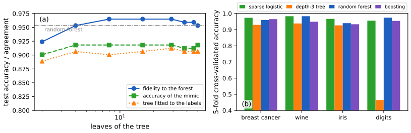
In panel (a) the mimic with four leaves already agrees with the forest on 95 percent of the 171 test points and the gap in accuracy (0.918 against 0.953) is below the bound \(1-\Fid=0.047\); trained on the forest's predictions the shallow tree is somewhat better than the same tree trained on the labels, in line with the book's remark that a complex model can teach a simple one. The gap is not significant at this test size, so I do not claim more.
33.3.2 Properties of explanations from cognitive science
p. 1089 Cognitive science and human-computer interaction have long studied what makes a human explanation good, and the chapter lists five properties with the ML property each corresponds to, while warning that human explanations are also social constructs full of post-hoc rationalisation: the properties to keep are those that help users reach their goals.
| Cognitive-science property | Meaning | Corresponds to |
|---|---|---|
| Soundness | nothing but the truth about what is described | compactness and faithfulness |
| Completeness | the whole truth about what is described | completeness and faithfulness |
| Generality | an explanation reflects a mechanism, so it applies to similar cases | stability |
| Simplicity | other things equal, prefer the simpler explanation | sparsity, complexity |
| Contrastiveness | how the outcome differs from an alternative | actionability, counterfactuals |
The chapter adds that explanations are goal-directed and take several forms in the human literature: deductive-nomological (a logical proof), a sense of underlying mechanism, and conveying understanding. Knowing these forms helps one choose among machine-learning explanation methods.
33.4 Evaluation of interpretable machine learning models
p. 1090 Interpretability cannot be defined without a context, an end-task and a downstream metric: an explanation is better if it lets the person do better. There are two kinds of evaluation. Computational evaluations of properties involve no people: they check whether an explanation has a property (faithfulness under different data distributions, sparsity) and serve as sanity checks before an expensive study. User studies measure whether the method helps people with the end-task. They are far more work than computing a test likelihood and the pool of experts can be tiny, but they can be done rigorously.
33.4.1 Computational evaluation: does the method have desired properties?
pp. 1090–1094 Checking properties catches implementation errors and odd behaviour, lets one iterate on a formalisation cheaply, shows whether a property that held for one model holds for another, and pinpoints how an explanation falls short (which a confounded user study cannot). Some properties can be proved; others need a test. Two umbrella strategies for tests:
- Hypothesis-based sanity checks: state "if the explanation works then phenomenon X should not occur", then try to produce X. If one can, the explanation fails the check; passing proves nothing (there may be blindspots).
- Data with known ground truth: purely synthetic data (tables with intentionally correlated features), semi-synthetic data (deliberately changed labels on an image set) or slices of real data (introduce bias by keeping only outdoor images).
Examples of sanity checks. (1) Adebayo et al. (2018) argue that a faithful explanation is a function of the model's prediction, so it should change a lot between a trained and an untrained (randomised) model; many saliency methods do not (Figure 33.4 in the book). (2) Kindermans et al. (2019) argue that an explanation should be invariant to input transformations that change neither predictions nor weights, such as adding a constant to all inputs; this tests faithfulness and stability together. (3) Adversarial attacks on explanations belong here too: two perceptually identical inputs with the same predicted label can be given very different explanations.
Semi-synthetic data. Yang and Kim (2019) test compactness and faithfulness with images in which each foreground object co-occurs with each background at a controlled rate, each image carrying an object label and a background label (Figure 33.3 in the book). A model trained to classify the object should give the background less importance than a model trained to classify the background (the model contrast score), and the background model should not credit the object.
Real data. Without ground truth one can still test a ranking: use only the top-1, top-2, ... features (or add image patches one at a time, Figure 33.5 in the book) and see whether accuracy shows diminishing returns; the reverse experiment deletes the top features. The test assumes the features do not interact. Dabkowski and Gal (2017) first define in words the smallest sufficient region and smallest destroying region, then operationalise them as optimisation objectives, and evaluate separately with a crop-and-classify metric. Finally, evaluations need evaluating: Tomsett et al. (2020) show that several popular saliency metrics are statistically unreliable and inconsistent with one another.
The two sanity checks and the insertion test can be made precise, and run.
Filling the gap 33.7: what the randomisation test and the shift test detect pp. 1091–1092
Derivation
Setting. An explanation method \(\mathcal E\) maps a model \(f\) and an input \(x\) to an explanation \(\mathcal E(f,x)\in\R^d\). The model-parameter randomisation test compares \(\mathcal E(f,x)\) for the trained model \(f\) with \(\mathcal E(f',x)\) for a copy \(f'\) whose parameters (all layers, or the last few) are re-drawn from the initialisation distribution, and asks for a measure of similarity (rank correlation of the importances) near zero. If the method were a faithful description of what the model computes, a model that computes something unrelated should be described differently.
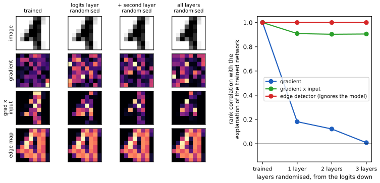
Linear model, gradient explanation. For \(f(x)=w^\T x+b\) the gradient explanation is \(w\). A re-initialised copy has \(w'\sim\N(0,s^2I_d)\), independent of \(w\). The cosine \(\cos\theta=w^\T w'/(|w||w'|)\) is the inner product of the fixed unit vector \(w/|w|\) with the uniformly distributed unit vector \(w'/|w'|\): it has the law of one coordinate of a uniform point on the sphere, so \(\E\cos\theta=0\) and \(\E\cos^2\theta=1/d\) (the squared coordinates sum to 1 and are exchangeable). For \(d=64\) the standard deviation is \(0.125\). The gradient explanation therefore passes: trained and randomised explanations are nearly orthogonal. In the digits experiment of figure x33.3, a three-layer network with 97 percent test accuracy has gradient explanations whose rank correlation with those of the trained network falls to 0.18, 0.12 and 0.01 as one, two and three layers are re-initialised.
An explanation that ignores the model fails. If \(\mathcal E(f,x)=e(x)\) depends on the input alone (an edge detector, the input itself) then \(\mathcal E(f,x)=\mathcal E(f',x)\) for every \(f'\): similarity 1, whatever the model. The check is a necessary condition for an explanation to be about the model, and a method can fail it by construction. Edge maps are in figure x33.3 for this reason: they look plausible on a digit and are unaffected by randomising the network.
Partial failure: gradient times input. For the linear model the attribution of feature \(j\) is \(w_jx_j\), of the randomised copy \(w'_jx_j\). In magnitude \(\log|w_jx_j|=\log|w_j|+\log|x_j|\) and \(\log|w'_jx_j|=\log|w'_j|+\log|x_j|\): the shared term \(\log|x_j|\) correlates the two. If \(w_j,w'_j,x_j\) are independent across features with the same law, the correlation of the log-magnitudes is \(V_x/(V_x+V_w)\), where \(V=\operatorname{var}\log|\cdot|\). For standard normal variables \(V=\pi^2/8\) for both and the correlation is \(1/2\); for digit images, where many pixels are exactly zero (their attribution is zero for every model) and the rest vary little, the rank correlation is much higher, 0.90 in the experiment. Gradient times input is therefore partly a description of the input.
Input shift. Let \(f(x)=\rho(Wx+b)\) with a first affine layer, and let model B have the same weights but bias \(b'=b+Wc\mathbf 1\) and receive inputs \(x'=x-c\mathbf 1\). Then \(Wx'+b'=Wx+b\): identical predictions on corresponding inputs, identical weights, and identical input gradients (the chain rule gives \(\partial f_B/\partial x'=\partial f/\partial x\)). The gradient explanation is invariant, but gradient times input is \(x\odot\partial f/\partial x\) for A and \((x-c\mathbf 1)\odot\partial f/\partial x\) for B, which differ by \(c\,\partial f/\partial x\), an arbitrary amount (in the numerical test with \(c=10\) the attributions differ by up to 1.7). A method that violates invariance to a change of input origin that leaves the model unchanged is reporting a fact about the origin.
Filling the gap 33.8: when insertion and deletion curves can be trusted, and how interactions break them p. 1093
Derivation
Setting. A ranking of features is tested by refitting a model on the top-\(k\) features (insertion curve, \(k=1,2,\dots\)) or on all features except the top-\(k\) (deletion curve). Write \(V(S)=\operatorname{var}\E[Y\given X_S]\) for the variance of the outcome explained by the subset \(S\); a better model on \(S\) cannot beat \(\E[Y\given X_S]\) in squared error, so \(V(S)\) is the natural score.
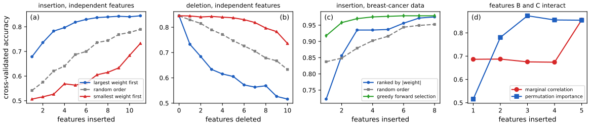
No interaction, independent features. Suppose \(Y=\sum_jg_j(X_j)+\varepsilon\) with independent features. Then \(\E[Y\given X_S]=\sum_{j\in S}g_j(X_j)+\const\), and by independence the variance of the sum is the sum of the variances: \[ V(S)=\sum_{j\in S}v_j,\qquad v_j=\operatorname{var}g_j(X_j). \] Order the features by \(v_{(1)}\ge v_{(2)}\ge\cdots\). The increments of the insertion curve \(V(\text{top-}k)=\sum_{i\le k}v_{(i)}\) are the non-increasing numbers \(v_{(k)}\): the curve is concave, with diminishing returns, and it is the highest curve among all rankings at every \(k\) (the sum of any \(k\) of the numbers is at most the sum of the \(k\) largest). The deletion curve \(V([d])-V(\text{top-}k)\) is convex and lowest. In this setting the test discriminates a good ranking from a bad one, as in figure x33.4 (a) and (b): ranking by the true weights in a 12-feature logistic model with independent features gives an insertion curve rising from 0.68 to 0.84 with diminishing steps, against a rise from 0.51 for the reverse order.
Interaction. If \(Y=BC\) with independent signs \(\pm1\), then \(\E[Y\given B]=B\,\E C=0\), so \(V(\{B\})=V(\{C\})=0\) while \(V(\{B,C\})=\operatorname{var}Y=1\): \(V\) is not additive, and the marginal importance of each is zero (their correlation with \(Y\) is 0, up to sampling error 0.006 and 0.03 in the simulation). A ranking by marginal importance puts \(B\) and \(C\) last, and the insertion curve stays flat until both are in, so it is not concave and the "diminishing returns" criterion is wrong for it. This is the book's example in which \(C\) matters only in the presence of \(B\). A permutation importance computed from a model fitted on all features does find the pair (gap 33.6 shows their Shapley values are equal), so it ranks them at the top: in figure x33.4 (d) with the extra feature \(A\), inserting by permutation importance gives accuracy 0.52 with one feature (B alone), 0.78 with two (B and C), 0.87 with three, against a flat 0.67 to 0.69 for marginal ranking until all five are inserted. The lesson: a faithful-looking curve is evidence only when the assumptions of the test (no interaction, no redundancy) hold. Redundancy is the other failure: in the breast-cancer data, which has strongly correlated features, ranking by the size of the logistic coefficients is worse for few features than a greedy forward selection (accuracy 0.72 against 0.92 with one feature, figure x33.4 (c)) although both rankings are reasonable descriptions of the fitted model; the weights of correlated features are unstable (gap 33.2).
33.4.2 User study-based evaluation: does the method help a user perform a target task?
p. 1094 A user study measures whether an explanation method helps a person with the end-task, or with a synthetic task that mirrors the context. Rigorous experimental design is essential.
33.4.2.1 User studies in real contexts
p. 1094 The gold standard is the intended context: do clinicians decide better with this decision support, do programmers debug faster with this explanation of model errors, do product teams build fairer models?
33.4.2.2 Basic elements of user studies
pp. 1094–1097 The book lists the following elements.
- Interface design. The explanation must be shown somehow. The intrinsic difficulty (complex models are harder to explain) must not be confounded with the extrinsic difficulty of the interface: a list sorted by importance is easier to scan than an alphabetical one. Training must be neutral across conditions, because how the task is described changes how people approach it.
- Baselines. The mere presence of an explanation changes behaviour. Compare with no ML system, an ML system with no explanation, with a placebo explanation (carrying no information), and with a hand-crafted explanation written by good communicators.
- Experimental design and hypothesis testing. Fix independent and dependent variables, hypotheses and inclusion and exclusion criteria before the study (for example, a developer's ability to find bugs as the dependent variable, with the explanation type and the baselines as the independent variable; exclude participants who are too inexperienced, disengaged, or already familiar with the explanation type; or whose completion times are extreme). Studies of the form "does explanation X help in context Z compared with X'" say little about why; manipulate the factors directly instead: write complete explanations by hand, explanations missing one important feature, and explanations missing several, or pretend to have a classifier with known bugs (wizard-of-Oz studies).
- Randomisation, matching and repeated measures. Randomisation marginalises confounds (prior knowledge, learning effects); matching (the same person does the task with both explanations) and repeated measures (several inputs per person) reduce variance. Block and Latin-square designs randomise the order of explanation types while keeping the tasks for one type together. Within-subject comparisons have lower variance but a possible bias from learning from the first task to the second; between-subject comparisons have higher variance and possible bias from population shift during recruitment. The design implies the test, and one must choose the right test and correct for multiple hypotheses, to avoid inflated significance while retaining power.
- Qualitative studies. Think-aloud protocols reveal why an explanation worked: for example, users watching video clips of a game agent might assume it always goes for coins, or put down its falling into a pit to a one-off slip instead of a systematic bug.
- Pilot studies. Small pilots find confusing instructions or unexpected use of the information, are discussed with the participants, and are excluded from the final results. As the number of factors grows so does the cost; pilots, think-alouds and careful thought about what can be settled computationally keep the study to the essential factors.
Three of these statements are statistical claims that can be stated and proved: that matching lowers variance (and by how much), that randomisation gives an unbiased comparison, and that the corrections the book mentions control the error rate.
Filling the gap 33.9: matching reduces variance by the factor \(1-\rho\); power of the two designs; order effects pp. 1096–1097
Derivation
Model. Participant \(i\) under condition \(k\in\{0,1\}\) scores \(Y_{ik}=\mu_k+s_i+\varepsilon_{ik}\), with a person effect \(s_i\) of variance \(\rho\sigma^2\) and noise \(\varepsilon_{ik}\) of variance \((1-\rho)\sigma^2\), all independent; so \(\operatorname{var}Y_{ik}=\sigma^2\) and the correlation between a person's two scores is \(\rho\). The effect is \(\delta=\mu_1-\mu_0\) and the standardised effect is \(d=\delta/\sigma\).
Between subjects (\(n\) different people per condition): \(\bar Y_1-\bar Y_0\) has variance \(2\sigma^2/n\), since the two groups are independent.
Within subjects (\(n\) people do both): the difference \(D_i=Y_{i1}-Y_{i0}=\delta+\varepsilon_{i1}-\varepsilon_{i0}\) has the person effect cancelled, \(\operatorname{var}D_i=2(1-\rho)\sigma^2\), and \(\bar D\) has variance \(2(1-\rho)\sigma^2/n\). Equivalently \(\operatorname{var}(Y_{i1}-Y_{i0})=2\sigma^2-2\operatorname{cov}=2\sigma^2(1-\rho)\). Pairing removes the shared person component and helps in proportion to \(\rho\); for \(\rho=0\) it removes nothing; for \(\rho<0\) it would hurt.
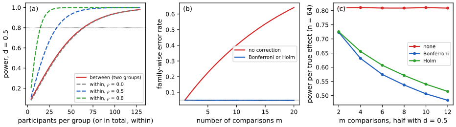
Power. With known \(\sigma\) the two-sided \(z\)-test at level \(\alpha\) has power \(\Phi(\lambda-z_{1-\alpha/2})+\Phi(-\lambda-z_{1-\alpha/2})\) where \(\lambda\) is the effect divided by the standard error: \(\lambda_{\text{between}}=d\sqrt{n/2}\), \(\lambda_{\text{within}}=d\sqrt{n/(2(1-\rho))}\). The two designs have the same noncentrality when \(n_{\text{within}}=(1-\rho)\,n_{\text{between}}\): a within-subject study needs about the fraction \(1-\rho\) of the per-group size of the between-subject study, which is a fraction \((1-\rho)/2\) of the \(2n\) people the between-subject study uses in total (each person is measured twice). With estimated variance the \(t\)-test uses the noncentral \(t\) distribution with \(2n-2\) degrees of freedom (between) or \(n-1\) (within); the exact numbers differ from the \(z\) approximation by a few units in small samples. For \(d=0.5\), \(\alpha=0.05\), power 0.8, the exact sizes are 64 per group between subjects and 34 people within (\(\rho=0.5\); the \(z\) rule predicts 32), 15 within for \(\rho=0.8\) (the rule: 13).
Order and learning effects. Suppose the second task done by anyone is \(\lambda\) higher because of practice. If everyone does condition 0 first the paired difference has mean \(\delta+\lambda\), biased. If half the people do (0,1) and half (1,0), the means are \(\delta+\lambda\) and \(\delta-\lambda\), and their average is \(\delta\): counterbalancing cancels the order effect exactly in the mean (and the order can then be entered as a covariate to remove the \(\lambda^2\) it adds to the variance). A Latin-square design extends this to several explanation types.
Filling the gap 33.10: randomisation marginalises confounders p. 1096
Derivation
Let unit \(i\) (a participant, a participant-task pair) have potential outcomes \(Y_i(0),Y_i(1)\) under the two conditions, treated as fixed numbers; the effect we want is \(\tau=\frac1n\sum_i(Y_i(1)-Y_i(0))\). Assign exactly \(n_1\) units to condition 1 uniformly at random: \(Z_i=1\) with probability \(n_1/n\) for every \(i\), \(n_0=n-n_1\). The difference in means is \[ \hat\tau=\frac1{n_1}\sum_iZ_iY_i(1)-\frac1{n_0}\sum_i(1-Z_i)Y_i(0), \] and since \(\E Z_i=n_1/n\) and \(\E(1-Z_i)=n_0/n\), \[ \E\hat\tau=\frac1{n_1}\cdot\frac{n_1}{n}\sum_iY_i(1)-\frac1{n_0}\cdot\frac{n_0}{n}\sum_iY_i(0)=\tau. \] The only property used is that the assignment is independent of the potential outcomes, so nothing about the units (prior knowledge of machine learning, optimism about AI, need for cognition) can bias the comparison: it averages out over the assignments. Randomising the order of tasks does the same for learning and fatigue. Enumerating all \(\binom84=70\) assignments of a set of 8 units confirms \(\E\hat\tau=\tau\) to machine precision. Randomisation does not make \(\hat\tau\) close to \(\tau\) in one study; that is the job of the sample size, and of the matching in gap 33.9.
Filling the gap 33.11: Bonferroni and Holm control the family-wise error p. 1096
Derivation
Setting. There are \(m\) hypotheses (for instance \(m\) explanation types each compared with a baseline), with \(p\)-values \(p_1,\dots,p_m\); let \(N\) be the set of true nulls, \(m_0=|N|\), and assume \(\Pr(p_i\le t)\le t\) for \(i\in N\) (valid tests). The family-wise error rate is \(\mathrm{FWER}=\Pr(\text{at least one true null is rejected})\). Testing each at level \(\alpha\) with no correction gives, for \(m\) independent true nulls, \(\mathrm{FWER}=1-(1-\alpha)^m\): 0.226 for \(m=5\), 0.40 for \(m=10\), 0.64 for \(m=20\).
Bonferroni. Reject \(H_i\) if \(p_i\le\alpha/m\). By the union bound (no independence needed) \[ \mathrm{FWER}=\Pr\Big(\bigcup_{i\in N}\{p_i\le\alpha/m\}\Big)\le\sum_{i\in N}\frac{\alpha}{m}=\frac{m_0}{m}\alpha\le\alpha. \] Under independence and the global null the exact value is \(1-(1-\alpha/m)^m\), e.g. 0.0489 for \(m=10\).
Holm. Order the \(p\)-values \(p_{(1)}\le\cdots\le p_{(m)}\) and reject \(H_{(1)},\dots,H_{(r)}\) where \(r\) is the largest index such that \(p_{(j)}\le\alpha/(m-j+1)\) for every \(j\le r\) (step down: stop at the first failure). Claim: \(\mathrm{FWER}\le\alpha\). Suppose some true null is rejected and let \(H_{(j^*)}\) be the first true null in the order. Before it come \(j^*-1\) false nulls, so \(j^*-1\le m-m_0\), that is \(m-j^*+1\ge m_0\). To reject \(H_{(j^*)}\) the procedure needs \(p_{(j^*)}\le\alpha/(m-j^*+1)\le\alpha/m_0\). Hence some true null has \(p_i\le\alpha/m_0\), and by the union bound over the \(m_0\) true nulls the probability is at most \(m_0\cdot\alpha/m_0=\alpha\). Holm rejects everything Bonferroni rejects: if \(p_{(j)}\le\alpha/m\) then also \(p_{(i)}\le\alpha/m\le\alpha/(m-i+1)\) for every \(i\le j\), so the step-down reaches \(j\). So Holm is uniformly at least as powerful, with the same guarantee and no extra assumptions. Under the global null (\(m_0=m\)) its first step is Bonferroni's, so the two have the same FWER there; with half of the nulls false (\(m=10\), \(d=0.5\), 64 per group) simulation gives power on the real effects of about 0.51 (Bonferroni) and 0.54 (Holm) against 0.81 uncorrected, and false-discovery rates among the true nulls of 0.03, 0.04 and 0.23.
The cost of correction is power: testing \(m\) hypotheses at level \(\alpha/m\) needs more participants for the same power. For \(d=0.5\), \(\alpha=0.05\) and \(m=5\), the per-comparison level is 0.01 and the between-subject sample size for 80 percent power rises from 64 to 96 per group (from 34 to 51 people matched at \(\rho=0.5\)).
33.4.2.3 User studies in synthetic contexts
pp. 1097–1098 Sometimes the real context is unavailable or unethical (one would not test a prototype on patients each time), so one uses made-up patients, an analogous non-medical task with a larger and cheaper pool, or a simplified image-debugging setting where labels and shifts are controlled. This can reveal general principles, such as how different forms of explanation load cognition, but there are cautions: subjects may not treat high stakes seriously, are free of the distractions of a hospital floor, may click through to finish, and small differences in the task definition have large effects (asking users to answer questions about the explanation first forces them to look at it). Priming with a scenario ("imagine you are an engineer at a company selling a risk calculator, a deadline is near...") helps put them in the right mindset.
33.5 Discussion: how to think about interpretable machine learning
pp. 1098–1102 The authors offer principles they expect to outlast the specifics of the previous sections.
- There is no universal mathematical definition of interpretability, and there never will be. What helps a clinician decide on a treatment policy differs from what helps an applicant get a loan approved, and from what suits models of text. One must define and justify a downstream metric for each context. Other areas lack a universal metric too (the fairness criteria cannot all hold at once; even for classification one chooses between accuracy, precision and recall), and evaluation stays rigorous so long as the assumptions are explicit. What is special here is that many evaluations need human input, so the work needs experimental design as well as computation and statistics.
- Interpretability is one part of a solution for fairness, calibrated trust, accountability, causality; those are goals and interpretability is a means.
- Sometimes it is not needed: when the goal can be fully formalised (a regulatory fairness metric), when a model behaves as expected on an exhaustive set of inputs, or when performance across regimes already gives the right amount of trust. Sometimes human input is needed: a dataset alone cannot guarantee a model is causal (compare Chapter 19, and Chapter 36), and waiting for harm to patients to show that a clinical system is unsafe is too late; inspecting the decision process beforehand can find red flags.
- Interpretability is about understanding enough to do the end-task, not understanding everything: a list of heat sources is enough to fix an overheating laptop and useless for a laptop that freezes. A Go expert can learn from partial probes of AlphaGo ("would this move have worked earlier in the game?") without understanding the whole network. It is also different from full transparency: reading every weight is like taking a laptop apart to debug a program.
- Any partial view is only partial. The features that would change a loan decision are the right view for the applicant and say nothing about whether the model discriminates. Incorrectly believing a partial view is the whole story gives incorrect insights.
- Partial views can lack stability and enable attacks. With over-parameterised models one can learn a model whose explanation says one thing (a feature is unimportant) while the model does another (uses the prohibited feature); joint training can make this worse; and inputs can be perturbed to change the explanation while keeping the prediction, or the reverse. The remedy the authors propose is translucence: explanations that say what they can and cannot say about the model.
- Trade-offs between inherently interpretable models and performance often do not exist. Data are often well fit by a simple model (noise is high), or by one that decomposes into interpretable parts; with the right architecture, regulariser and optimiser interpretable models can match or beat black boxes; sparsity regularisers were invented to improve performance; and a predefined validation metric may not tell the full story (a person inspecting an interpretable model may see that a prediction rests on confounding, and can override the system in teaming). Where a gap does exist, partial views help.
- Human factors are essential. Over-reliance: the presence of an explanation raises trust even among data scientists, and an evocative but inaccurate picture creates a feeling of understanding; remedies force analytical engagement (ask for the user's decision before showing the recommendation, ask questions about the explanation, or show the explanation without the recommendation), at the risk that too much effort leads users to ignore the information. Potential for misuse: explanations can manipulate, and people like simple explanations even when they do not help. Misunderstanding of machine learning: not everyone knows what an additive factor or a Shapley value is, and highlighting a beak or a set of disease words suggests concepts the model need not have. Perception issues in image explanations (Figure 33.6 in the book, not reproduced): a saliency map from a trained network and one from an untrained network look alike to a person because people see a bird, not pixel values, even though the maps differ numerically (in figure x33.3 the gradient maps of the trained and the randomised network are numerically unrelated, whereas the gradient-times-input maps keep the shape of the digit and would reassure a viewer looking for a digit-shaped blob); multiplying the image by an importance mask makes black objects never look important; and clipping to a percentile adds another artefact. Balancing readability against faithfulness remains a challenge.
Panel (b) of figure x33.5 gives a small quantitative illustration of the no-trade-off point: on the breast-cancer, wine and iris data an L1-regularised logistic regression is as accurate as a random forest or boosting (0.974, 0.983 and 0.967 against 0.960, 0.983 and 0.940 for the forest), whereas on the 10-class digits it is about two points behind (0.956 against 0.974) and a depth-3 tree is far behind (0.46): the claim is not that a simple model always suffices, but that the accuracy cost of an inspectable model is often small and has to be measured.
Supplement S33 (Interpretability)
The supplement's Chapter 33 consists of the chapter title only (page 303); there is no additional material for this chapter in the draft.
Practice problems
The book has no exercises for this chapter. These three short problems are my own.
Practice problem 33.1 (units). In Model 2 of (33.2) with \(\max T=100\) the temperature is measured in units of \(u_0=10\) degrees. What is the ratio of the mean absolute derivatives with respect to temperature and cleanliness? At which unit \(u_0\) do the two importances coincide?
Solution
With \(\theta=T/u_0\) the derivative is \(\partial p/\partial\theta=u_0\,\partial p/\partial T=u_0\cdot\frac{0.9}{\max T}p(1-p)\), while \(\partial p/\partial c=0.1\,p(1-p)\) (gap 33.1). The ratio is the same on every day, \(\frac{9u_0}{\max T}\); for \(u_0=10\), \(\max T=100\) it is \(0.9\): cleanliness is still (slightly) ahead. They coincide when \(9u_0=\max T\), \(u_0=11.1\) degrees. Numerically, the mean absolute derivatives on the 400-day design are 0.0224 (temperature in units of 10 degrees) and 0.0249 (cleanliness): ratio 0.900.
Practice problem 33.2 (a local explanation of a cube). In one dimension, fit a line to \(f(x)=x^3\) around \(x_0=0\) with Gaussian weights of width \(h\). What slope does the surrogate report, and how does it compare with the derivative at 0?
Solution
By gap 33.4 the slope is \[ b=h^{-2}\E[u\,f(u)]=h^{-2}\E[u^4]=h^{-2}\cdot3h^4=3h^2, \] because \(\E u^4=3h^4\) for \(u\sim\N(0,h^2)\). The derivative at 0 is \(f'(0)=0\). So the explanation depends on the neighbourhood: it says "no effect" as \(h\to0\) and slope 3 at \(h=1\); the bias \(\frac{h^2}{2}f'''=3h^2\) of gap 33.4 is exact here (the fourth-order remainder vanishes for a cubic). A direct weighted least-squares fit on a fine grid reproduces \(3h^2\) (0.27 for \(h=0.3\)).
Practice problem 33.3 (sample size for five explanation types). A study compares each of \(m=5\) explanation types with a baseline, expecting a standardised effect \(d=0.5\) for each, and wants 80 percent power per comparison at overall level 0.05 (Bonferroni). How many participants per group are needed between subjects, and how many people if the same people see both conditions with \(\rho=0.5\)? Compare with a single comparison.
Solution
Bonferroni tests each comparison at level \(0.05/5=0.01\), so FWER \(\le0.05\) (gap 33.11). The exact power of the two-sided \(t\)-test uses the noncentrality \(d\sqrt{n/2}\) with \(2n-2\) degrees of freedom (between) or \(d\sqrt{n/(2(1-\rho))}\) with \(n-1\) (within); searching \(n=3,4,\dots\) for the first \(n\) with power at least 0.8 gives 96 per group at level 0.01, against 64 per group at level 0.05, and 51 matched people against 34. Correcting for five comparisons costs 50 percent more participants in both designs. At \(n=64\) per group the power per comparison under the correction falls from 0.80 to 0.59.
Notes on the book
The derivative ranking in the lemonade example depends on the units p. 1078
The text says that for Model 2 the second explanation "will still report that temperature has higher derivatives", while the temperature is introduced as measured in degrees Fahrenheit. Differentiating (33.2) with respect to the temperature in degrees gives \((0.9/\max T)\,p(1-p)\), which is \(\max T/9\) times smaller than the derivative with respect to cleanliness: with \(\max T=100\) the mean absolute derivatives are 0.0022 and 0.0249 on a 400-day design, so the cleanliness would be named. The statement is correct only if the derivative is taken with respect to \(T/\max T\) (0.224 against 0.025). The qualitative lesson, that the two methods can disagree on models with the same behaviour, is unaffected (and is strengthened by the units dependence); gap 33.1 gives the exact ratios.
Model 2 as printed is almost flat p. 1077, Equation (33.2)
With \(\max T\) the largest temperature (about 100) the argument of \(\sigma\) in (33.2) lies between \(-0.28\) and \(0.28\) over the stated ranges of the inputs, so \(p(\text{profit})\) only varies between about 0.43 and 0.57 (Figure 33.2 in these notes, panel b). Such a model cannot fit data that a step in (33.1) fits well, in which the probability jumps from at most 0.1 to at least 0.9; "two models seem to fit the data approximately equally well" needs a steeper sigmoid, for instance a factor \(k\) in front of the argument (the demonstration lets you choose \(k\); \(k=20\) gives a model that behaves like Model 1). It does not change the point of the example.
References
- Murphy, K. P. (2023). Probabilistic Machine Learning: Advanced Topics. MIT Press, Cambridge, MA. Chapter 33, pp. 1073–1102 (by B. Kim and F. Doshi-Velez). probml.github.io/pml-book/book2.html.
- Adebayo, J., Gilmer, J., Muelly, M., Goodfellow, I., Hardt, M. and Kim, B. (2018). Sanity checks for saliency maps. Advances in Neural Information Processing Systems 31.
- Bonferroni, C. E. (1936). Teoria statistica delle classi e calcolo delle probabilità. Pubblicazioni del R. Istituto Superiore di Scienze Economiche e Commerciali di Firenze, 8, 3–62.
- Dabkowski, P. and Gal, Y. (2017). Real time image saliency for black box classifiers. Advances in Neural Information Processing Systems 30.
- Doshi-Velez, F. and Kim, B. (2017). Towards a rigorous science of interpretable machine learning. arXiv:1702.08608.
- Hinton, G., Vinyals, O. and Dean, J. (2015). Distilling the knowledge in a neural network. arXiv:1503.02531.
- Holm, S. (1979). A simple sequentially rejective multiple test procedure. Scandinavian Journal of Statistics, 6, 65–70.
- Kindermans, P.-J., Hooker, S., Adebayo, J., Alber, M., Schütt, K. T., Dähne, S., Erhan, D. and Kim, B. (2019). The (un)reliability of saliency methods. In Explainable AI: Interpreting, Explaining and Visualizing Deep Learning, Springer.
- Lundberg, S. M. and Lee, S.-I. (2017). A unified approach to interpreting model predictions. Advances in Neural Information Processing Systems 30.
- Ribeiro, M. T., Singh, S. and Guestrin, C. (2016). "Why should I trust you?": explaining the predictions of any classifier. Proceedings of the 22nd ACM SIGKDD Conference.
- Rudin, C. (2019). Stop explaining black box machine learning models for high stakes decisions and use interpretable models instead. Nature Machine Intelligence, 1, 206–215.
- Shapley, L. S. (1953). A value for n-person games. In Contributions to the Theory of Games II, Princeton University Press, 307–317.
- Smilkov, D., Thorat, N., Kim, B., Viégas, F. and Wattenberg, M. (2017). SmoothGrad: removing noise by adding noise. arXiv:1706.03825.
- Stein, C. M. (1981). Estimation of the mean of a multivariate normal distribution. Annals of Statistics, 9, 1135–1151.
- Tomsett, R., Harborne, D., Chakraborty, S., Gurram, P. and Preece, A. (2020). Sanity checks for saliency metrics. Proceedings of the AAAI Conference on Artificial Intelligence, 34.
- Yang, M. and Kim, B. (2019). Benchmarking attribution methods with relative feature importance. arXiv:1907.09701.
The numerical statements in the text (the exact flip and derivative importances of the lemonade models and their dependence on the units, the Gaussian-smoothing form of the local surrogate and its small-neighbourhood expansion, the fidelity and Lipschitz formulas, the Shapley values, the variance of least-squares weights under correlation, the randomisation and shift tests, the insertion-curve claims, the power calculations, the sample sizes and the error rates of Bonferroni and Holm) were confirmed numerically.