Generalized linear models
A generalized linear model (GLM) is a conditional exponential family whose natural parameter is linear in the inputs. This chapter turns the GLM into a Bayesian tool: closed-form posteriors for linear regression, priors that induce shrinkage and sparsity (spike and slab, Laplace, horseshoe, automatic relevancy determination), Laplace, variational and Monte Carlo posteriors for logistic and probit regression, and hierarchical (multilevel) GLMs. The notes prove what the book states, check it numerically, and reproduce its figures on simulated or bundled data.
Ch. 1 Introduction Ch. 2 Probability Ch. 3 Statistics Ch. 4 Graphical models Ch. 5 Information theory Ch. 6 Optimisation Ch. 7 Inference algorithms Ch. 8 Gaussian filtering Ch. 9 Message passing Ch. 10 Variational inference Ch. 11 Monte Carlo Ch. 12 MCMC Ch. 13 Sequential Monte Carlo Ch. 14 Predictive models Ch. 15 GLMs Ch. 16 Deep networks Ch. 17 Bayesian neural networks Ch. 18 Gaussian processes Ch. 19 Beyond iid Ch. 20 Generative models Ch. 21 VAEs Ch. 22 Autoregressive models Ch. 23 Normalizing flows Ch. 24 Energy-based models Ch. 25 Diffusion models Ch. 26 GANs Ch. 27 Discovery methods Ch. 28 Latent factor models Ch. 29 State-space models Ch. 30 Graph learning Ch. 31 Nonparametric Bayes Ch. 32 Representation learning Ch. 33 Interpretability Ch. 34 Decision making Ch. 35 Reinforcement learning Ch. 36 Causality
How to read these notes
They follow the book. Sections carry the book's numbers and equations keep theirs (for example (15.57) or (15.149)); equations of the supplement are written (S15.4) and so on. The supplement's three sections are placed where they belong and labelled "(supplement)": the variational bounds with the other approximate-inference methods (15.3.8), Poisson and beta-binomial regression with the Berkeley case study (15.3.9), and the hierarchical model of the same data at the end (15.5).
Filling the gaps. Wherever the book states a result without proof, an orange Filling the gap box gives the full argument. Proofs start hidden. Results already proved in the introductory volume (Newton's method for logistic regression, ridge and lasso, binomial and Poisson regression) are linked, not repeated.
Figures and data. The book's data files are not available. The height-weight data of Figures 15.1 and 15.2 and the radon data of Figures 15.15 to 15.17 are replaced by simulations with the same structure (the captions say so), Figure 15.8 uses the iris data, Figure 15.9 uses the twelve counts of Table 15.1, and the rest are simulated. Sampling is done with a Hamiltonian Monte Carlo sampler written for this course (hmc in the code), checked against grid integration.
Main reference
K. P. Murphy, Probabilistic Machine Learning: Advanced Topics, MIT Press (2023; December 2025 draft), Chapter 15, pages 591–630, and the online supplement, Chapter 15, pages 161–172 (book page: probml.github.io/pml-book/book2.html). The book has no exercises for this chapter; three practice problems are at the end.
Companion courses
- Probabilistic Machine Learning: An Introduction: Chapter 12 generalized linear models (12.4 maximum likelihood), 10.5 Bayesian logistic regression, 11.7 Bayesian linear regression (including ARD), 11.4 lasso.
- Bayesian and Probabilistic Machine Learning: 3.3 Bayesian linear regression, 3.5 the evidence approximation, 4.5 Bayesian logistic regression, 7.2 relevance vector machines, 10.6 variational logistic regression.
- Introduction to Statistical Learning: Chapter 4 classification, Chapter 6 regularisation. All of Statistics: Chapter 13 regression.
- This course: 3.5.2 Jeffreys priors, 7.4.3 Laplace approximation, 12.5 Hamiltonian Monte Carlo, 12.6.5 non-centred parameterisations, 14.1.3 generalised Bayes.
What this chapter adds: the Bayesian treatment of GLMs (priors on the logit scale, sparsity-inducing and marginal-likelihood priors, Laplace, variational and sampling posteriors with their predictive approximations), probit regression as a latent-variable model with EM and Gibbs, and the hierarchical and mixed-effects extension.
The chapter at a glance
- 15.1 GLMs as conditional exponential families, links, maximum likelihood (gaps 15.1 to 15.3).
- 15.2 Bayesian linear regression: the normal-inverse-gamma posterior, Jeffreys and g-priors (gaps 15.4 to 15.6), spike and slab, Bayesian lasso, horseshoe (gaps 15.8 to 15.10), automatic relevancy determination (gaps 15.11 to 15.13) and the matrix-normal inverse-Wishart model (gap 15.14).
- 15.3 Logistic regression: logit adjustment (gap 15.15), priors on the logit scale (gap 15.16), Laplace posterior and the probit approximation of the predictive (gaps 15.17, 15.18), HMC, the variational bounds of the supplement (gaps 15.19, 15.20), the Berkeley case study and Simpson's paradox, Poisson and beta-binomial regression (gaps 15.21 to 15.23).
- 15.4 Probit regression: latent variables, EM, Gibbs, ordinal models (gaps 15.24 to 15.26).
- 15.5 Hierarchical GLMs, partial pooling, the radon example and the non-centred parameterisation (gaps 15.27 to 15.29).
Notation. Inputs \(x_n\in\R^D\), natural parameter \(\eta_n=w^\T x_n\), mean \(\mu_n=\E[y_n]\), \(\sigma(a)=1/(1+e^{-a})\), \(\Phi\) and \(\phi\) the standard normal cdf and density, \(\mathrm{N}(\cdot\given m,V)\) a Gaussian density. In the book \(\N(m,s)\) for scalars such as "\(\N(0,1.5)\)" is mean and standard deviation; the notes say so whenever it matters.
15.1 Introduction
p. 591 A GLM is a conditional version of an exponential family: \[ p(y_n\given x_n,w,\sigma^2)=\exp\!\Big\{\frac{y_n\eta_n-A(\eta_n)}{\sigma^2}+\log h(y_n,\sigma^2)\Big\},\qquad\eta_n=w^\T x_n, \tag{15.1} \] with log normaliser \(A\), sufficient statistic \(y_n\) and dispersion \(\sigma^2\). The mean and variance are \[ \mu_n=\E[y_n]=A'(\eta_n)=\ell^{-1}(\eta_n)\ \ (15.2),\qquad \var[y_n]=A''(\eta_n)\,\sigma^2\ \ (15.3), \] and the link function \(\ell\) satisfies \(\ell(\mu_n)=\eta_n=w^\T x_n\) (15.4). GLMs are weak predictors (they are linear, apart from the link) but they are the standard tool for hypothesis testing, which needs the posterior \(p(w\given\mathcal D)\) of Section 15.1.4.
Filling the gap 15.1: the mean and variance of a GLM, and of the zero-inflated Poisson pp. 591–594
Derivation
Moments from \(A\). Fix \(x_n\) and write \(\eta=\eta_n\), \(\sigma^2\) known. Normalisation says \(\int e^{y\eta/\sigma^2}h(y,\sigma^2)\,\d y=e^{A(\eta)/\sigma^2}\) for every \(\eta\) in the interior of the natural parameter space. In this interior differentiation under the integral sign is allowed (the integrand and its \(\eta\)-derivatives are dominated locally uniformly by integrable functions, a standard property of exponential families). The first derivative gives \(\int\frac{y}{\sigma^2}e^{y\eta/\sigma^2}h\,\d y=\frac{A'(\eta)}{\sigma^2}e^{A(\eta)/\sigma^2}\); dividing by \(e^{A/\sigma^2}\), \(\E[y]=A'(\eta)\). The second derivative gives \(\E[y^2]/\sigma^4=A''/\sigma^2+(A')^2/\sigma^4\), so \(\var[y]=\E y^2-(A')^2=\sigma^2A''(\eta)\). Since \(\var[y]>0\), \(A''>0\): \(A\) is strictly convex and \(A'\) is strictly increasing, hence invertible, so \(\ell=(A')^{-1}\) is well defined.
The three examples. Gaussian: \(A=\eta^2/2\), \(A'=\eta\), \(A''=1\), variance \(\sigma^2\). Binomial with \(N_n\) trials: \(A=N_n\log(1+e^\eta)\), \(A'=N_n\sigma(\eta)\), \(A''=N_n\sigma(\eta)(1-\sigma(\eta))\) because \(\sigma'=\sigma(1-\sigma)\). Poisson: \(A=e^\eta\), \(A'=A''=e^\eta\). (These are also proved in the introductory volume, 12.2.)
The zero-inflated Poisson (15.24). It is the mixture "spike at 0 with probability \(\rho\), otherwise Poisson(\(\lambda\))", so it is not itself an exponential-family GLM, but its moments are immediate. \(\E[y]=(1-\rho)\lambda\). \(\E[y^2]=(1-\rho)(\lambda+\lambda^2)\), hence \(\var[y]=(1-\rho)(\lambda+\lambda^2)-(1-\rho)^2\lambda^2=(1-\rho)\lambda(1+\rho\lambda)\), which exceeds the Poisson variance \((1-\rho)\lambda\) by \(\rho(1-\rho)\lambda^2\): zero inflation is a source of overdispersion. In a regression one sets \(\log\lambda_n=w^\T x_n\) and \(\logit\rho_n=v^\T x_n\) (two linear predictors). Both identities are confirmed numerically by summing the pmf.
15.1.1 Some popular GLMs
pp. 591–594 Linear regression has \(A(\eta)=\eta^2/2\) and \(\sigma^2\) the noise variance (15.5)–(15.9). Binomial regression models counts \(y_n\in\{0,\dots,N_n\}\) with \(\mu_n=\sigma(w^\T x_n)\), log-pdf \(y_n\eta_n-N_n\log(1+e^{\eta_n})+\log\binom{N_n}{y_n}\) and mean and variance (15.16), (15.17); binary logistic regression is \(N_n=1\). Poisson regression models counts with \(\mu_n=\exp(w^\T x_n)\) (15.18)–(15.23). The zero-inflated Poisson adds a spike: \[ \mathrm{ZIP}(y\given\rho,\lambda)=\begin{cases}\rho+(1-\rho)e^{-\lambda}&y=0,\\(1-\rho)\,\dfrac{\lambda^ye^{-\lambda}}{y!}&y>0.\end{cases}\tag{15.24} \] A zero can come from the spike (probability \(\rho\)) or from the Poisson (probability \(e^{-\lambda}\)). See also the introductory volume: 12.2.2 binomial, 12.2.3 Poisson.
15.1.2 GLMs with noncanonical link functions
p. 594 The canonical link is \(\ell=(A')^{-1}\), so that \(\theta=\ell(\mu)=\eta\): the linear predictor is the natural parameter (logit for the Bernoulli, log for the Poisson). Other links are allowed. The probit link \(\ell(\mu)=\Phi^{-1}(\mu)\) (15.28), (15.29) is the subject of Section 15.4. The complementary log-log link \(\ell(\mu)=\log(-\log(1-\mu))\) (15.30) arises when \(y=1\) means "at least one event" of a Poisson process of rate \(\lambda=e^{\eta}\): then \(1-\mu=\Pr(y=0)=e^{-\lambda}\) (15.31), so \(\lambda=-\log(1-\mu)\) and \(\eta=\log\lambda\) (15.32).
Filling the gap 15.2: the cloglog inverse link and what its coefficients mean p. 594
Derivation
Inverting (15.30): \(\eta=\log(-\log(1-\mu))\iff e^\eta=-\log(1-\mu)\iff\mu=1-\exp(-e^{\eta})\). Writing \(\lambda=e^{\eta}=e^{w^\T x}\), a unit increase of \(x_d\) multiplies the event rate \(\lambda\) by \(e^{w_d}\); in logistic regression it multiplies the odds \(\mu/(1-\mu)\) by \(e^{w_d}\). For rare events \(\mu\approx\lambda\) and the two coincide; as \(\eta\to+\infty\) the cloglog probability approaches 1 doubly exponentially fast, \(1-\mu=\exp(-e^\eta)\), faster than the logistic \(1-\mu\approx e^{-\eta}\), and as \(\eta\to-\infty\) it behaves like \(e^{\eta}\), the same as the logistic: the link is asymmetric. A numerical round trip confirms the inversion.
15.1.3 Maximum likelihood estimation
p. 595 With \(\sigma^2=1\), \(\NLL(w)=-\sum_n\ell_n\), \(\ell_n=\eta_ny_n-A(\eta_n)\) (15.33), (15.34). For the canonical link the gradient and Hessian are \[ g_n=(y_n-\mu_n)\,x_n\ (15.35),\qquad H=\sum_{n=1}^Nf'(\eta_n)\,x_nx_n^\T\ (15.38),\quad f=A'=\ell^{-1}. \] Since \(f'(\eta_n)=A''(\eta_n)>0\), the Hessian is positive definite when \(X\) has full column rank, so \(\NLL\) is strictly convex and the MLE is unique if it exists (the book writes "\(f(\eta_n)>0\)" where \(f'(\eta_n)>0\) and the rank condition are meant). Small data sets use IRLS (Newton), large ones SGD; see the introductory volume, 10.2.6.
Filling the gap 15.3: gradient, Hessian, convexity and IRLS for a GLM; Fisher scoring for other links p. 595
Derivation
Canonical link. \(\partial\ell_n/\partial\eta_n=y_n-A'(\eta_n)=y_n-\mu_n\) and \(\partial\eta_n/\partial w=x_n\), giving (15.35). Differentiating again, \(\partial^2\ell_n/\partial w\partial w^\T=-A''(\eta_n)x_nx_n^\T\), and \(A''=f'\) because \(f=A'\): this is (15.38) for the Hessian of \(\NLL\). For any \(v\ne0\), \(v^\T Hv=\sum_nA''(\eta_n)(x_n^\T v)^2\ge0\), with equality only if \(Xv=0\); so \(H\succ0\) iff \(\operatorname{rank}X=D\).
IRLS. The Newton step is \(w^{+}=w+H^{-1}X^\T(y-\mu)\). Put \(S=\diag(f'(\eta_n))\) and the working response \(z=Xw+S^{-1}(y-\mu)\). Then \(w^{+}=(X^\T SX)^{-1}X^\T S\,(Xw+S^{-1}(y-\mu))=(X^\T SX)^{-1}X^\T Sz\): a weighted least-squares fit to \(z\), repeated with updated weights (this is IRLS; see 10.2.6). A convex objective with positive definite Hessian has at most one minimiser; whether it exists depends on the data (Section 15.3.5 and gap 15.17 for separable logistic data). The own implementation agrees with the library fit to \(10^{-15}\).
Non-canonical link. If \(\eta=\ell(\mu)\) with \(\ell\ne(A')^{-1}\), the score is \(\sum_n\frac{(y_n-\mu_n)}{V(\mu_n)}\frac{\d\mu_n}{\d\eta_n}x_n\) (with \(V=A''\), \(\sigma^2=1\)) and the observed Hessian contains an extra term proportional to \((y_n-\mu_n)\), so it can lose positive definiteness. Replacing it by its expectation (the Fisher information) removes that term because \(\E[y_n-\mu_n]=0\): \(\mathcal I=\sum_n\frac{(\d\mu_n/\d\eta_n)^2}{V(\mu_n)}x_nx_n^\T\succeq0\). Newton with \(\mathcal I\) is Fisher scoring; for the canonical link \(\d\mu/\d\eta=V\) and \(\mathcal I=H\) exactly, so scoring and Newton coincide.
15.1.4 Bayesian inference
pp. 595–596 Point estimates give no uncertainty, which hypothesis testing and regularisation both need. A Bayesian analysis needs a prior chosen with the link in mind: a flat prior on a logit offset is far from flat on the probability scale (Section 15.3.4). Posteriors can be computed by HMC (Chapter 12.5), which only needs the log joint and its gradient, by software built on it (Bambi, RStanARM, BRMS, all with the formula syntax), or, for large data, by variational inference, expectation propagation and related methods. The rest of the chapter does this case by case.
15.2 Linear regression
p. 596 The simplest GLM is \(p(y\given x,\theta)=\N(y\given w_0+w^\T x,\sigma^2)\) (15.39), \(\theta=(w_0,w,\sigma^2)\). The book briefly recalls maximum likelihood and then develops the Bayesian analysis. See also the introductory volume, 11.7 and ml 3.3.
15.2.1 Ordinary least squares
pp. 596–597 The negative log likelihood is \(\NLL(w,\sigma^2)=\frac1{2\sigma^2}\sum_n(y_n-\hat y_n)^2+\frac N2\log(2\pi\sigma^2)\) (15.41), minimised by the OLS estimate \(\hat w_{\rm mle}=(X^\T X)^{-1}X^\T y\) (15.42) and \(\hat\sigma^2_{\rm mle}=\frac1N\sum_n(y_n-x_n^\T\hat w)^2\) (15.43); the proof is in 11.2.2.
15.2.2 Conjugate priors
pp. 597–599 Known noise variance. With prior \(p(w)=\N(w\given\breve w,\breve\Sigma)\) (15.44), Bayes' rule for Gaussians gives \[ p(w\given X,y,\sigma^2)=\N(w\given\hat w,\hat\Sigma),\quad \hat\Sigma=\big(\breve\Sigma^{-1}+\tfrac1{\sigma^2}X^\T X\big)^{-1}\ (15.48),\quad \hat w=\hat\Sigma\big(\breve\Sigma^{-1}\breve w+\tfrac1{\sigma^2}X^\T y\big)\ (15.47). \] With \(\breve w=0\), \(\breve\Sigma=\tau^2I\): \(\hat w=(\frac{\sigma^2}{\tau^2}I+X^\T X)^{-1}X^\T y\) (15.49), which is ridge regression with \(\lambda=\sigma^2/\tau^2\) (15.50).
Unknown noise variance. The conjugate prior is the normal-inverse-gamma \[ \mathrm{NIG}(w,\sigma^2\given\breve w,\breve\Sigma,\breve a,\breve b)=\N(w\given\breve w,\sigma^2\breve\Sigma)\,\IG(\sigma^2\given\breve a,\breve b),\quad\IG(\sigma^2\given a,b)=\tfrac{b^a}{\Gamma(a)}(\sigma^2)^{-(a+1)}e^{-b/\sigma^2},\tag{15.53-15.55} \] and the posterior is NIG with \(\hat\Sigma=(\breve\Sigma^{-1}+X^\T X)^{-1}\) (15.59), \(\hat w=\hat\Sigma(\breve\Sigma^{-1}\breve w+X^\T y)\) (15.58), \(\hat a=\breve a+N/2\) (15.60), \(\hat b=\breve b+\frac12(\breve w^\T\breve\Sigma^{-1}\breve w+y^\T y-\hat w^\T\hat\Sigma^{-1}\hat w)\) (15.61). The marginals are \(p(\sigma^2\given\mathcal D)=\IG(\hat a,\hat b)\) (15.62) and the Student \(p(w\given\mathcal D)=\mathcal T(w\given\hat w,\frac{\hat b}{\hat a}\hat\Sigma,2\hat a)\) (15.63).
Filling the gap 15.4: the NIG posterior, its Student marginal and the posterior predictive (15.57)–(15.66) pp. 597–599
Derivation
Posterior. Up to constants, prior times likelihood is \((\sigma^2)^{-(\breve a+D/2+1)-N/2}\exp\{-[\breve b+\frac12Q(w)]/\sigma^2\}\) with \(Q(w)=(w-\breve w)^\T\breve\Sigma^{-1}(w-\breve w)+\|y-Xw\|^2\). Expand \(Q\) and complete the square: \[ Q(w)=w^\T(\breve\Sigma^{-1}+X^\T X)w-2w^\T(\breve\Sigma^{-1}\breve w+X^\T y)+\breve w^\T\breve\Sigma^{-1}\breve w+y^\T y=(w-\hat w)^\T\hat\Sigma^{-1}(w-\hat w)+\big[\breve w^\T\breve\Sigma^{-1}\breve w+y^\T y-\hat w^\T\hat\Sigma^{-1}\hat w\big]. \] So the posterior is proportional to \((\sigma^2)^{-(\hat a+D/2+1)}\exp\{-[\hat b+\frac12(w-\hat w)^\T\hat\Sigma^{-1}(w-\hat w)]/\sigma^2\}\) with \(\hat a=\breve a+N/2\) and \(\hat b\) as in (15.61): this is \(\mathrm{NIG}(\hat w,\hat\Sigma,\hat a,\hat b)\).
Marginals. Integrating the Gaussian in \(w\) gives \((2\pi\sigma^2)^{D/2}|\hat\Sigma|^{1/2}\), which removes the factor \((\sigma^2)^{D/2}\) and leaves \((\sigma^2)^{-(\hat a+1)}e^{-\hat b/\sigma^2}\): \(\IG(\hat a,\hat b)\), (15.62). Integrating \(\sigma^2\) instead, with \(\int_0^\infty s^{-(c+1)}e^{-B/s}\d s=\Gamma(c)B^{-c}\) and \(c=\hat a+D/2\), gives \(p(w\given\mathcal D)\propto[1+\frac{(w-\hat w)^\T\hat\Sigma^{-1}(w-\hat w)}{2\hat b}]^{-(\hat a+D/2)}\). A multivariate Student \(\mathcal T(\mu,\Sigma_t,\nu)\) is proportional to \([1+\frac1\nu(w-\mu)^\T\Sigma_t^{-1}(w-\mu)]^{-(\nu+D)/2}\); matching exponents gives \(\nu=2\hat a\) and \(\Sigma_t^{-1}/\nu=\hat\Sigma^{-1}/(2\hat b)\), i.e. \(\Sigma_t=\frac{\hat b}{\hat a}\hat\Sigma\): (15.63).
Predictive. Given \(\sigma^2\), a new output \(\tilde y=\tilde x^\T w+\varepsilon\) with \(w\given\sigma^2,\mathcal D\sim\N(\hat w,\sigma^2\hat\Sigma)\) and independent \(\varepsilon\sim\N(0,\sigma^2)\) is \(\N(\tilde x^\T\hat w,\sigma^2(1+\tilde x^\T\hat\Sigma\tilde x))\). This is a Gaussian with variance \(\sigma^2c\), \(c=1+\tilde x^\T\hat\Sigma\tilde x\), mixed over \(\sigma^2\sim\IG(\hat a,\hat b)\); the same integral as above shows the scale mixture is a Student with \(2\hat a\) degrees of freedom and squared scale \(\frac{\hat b}{\hat a}c\). For \(N'\) test points the argument is the same with \(I_{N'}+\tilde X\hat\Sigma\tilde X^\T\): (15.66). The two variance components are \(\frac{\hat b}{\hat a}\) (noise) and \(\frac{\hat b}{\hat a}\tilde x^\T\hat\Sigma\tilde x\) (parameter uncertainty, which grows away from the data). Plugging in a point estimate of \(\sigma^2\) replaces the Student by a Gaussian with thinner tails. A Monte Carlo draw of \((w,\sigma^2,\tilde y)\) reproduces the Student quantiles to three decimals.
See also: 3.4.3.3 the conjugate NIG prior for the Gaussian; 11.7.2 posteriors.
15.2.3 Uninformative priors
pp. 599–601 Jeffreys prior. \(p(w)\propto1\) and \(p(\sigma)\propto\sigma^{-1}\) (3.5.2) are emulated by the improper NIG with \(\breve\Sigma^{-1}\to0\), \(\breve a=-D/2\), \(\breve b=0\), giving \(\hat w=\hat w_{\rm mle}\), \(\hat\Sigma=(X^\T X)^{-1}=C\), \(\hat a=\nu/2\), \(\hat b=s^2\nu/2\) with \(\nu=N-D\), \(s^2=\|y-\hat y\|^2/\nu\) (15.67)–(15.73), so \(p(w_d\given\mathcal D)=\mathcal T(w_d\given\hat w_d,s^2C_{dd},\nu)\) (15.74), (15.75). Connection to frequentist statistics. This posterior equals the sampling distribution of the MLE, \((\hat w_d-w_d)/(s\sqrt{C_{dd}})\sim t_{N-D}\) (15.76), (15.77), because the Student density is symmetric in its argument and location, but the two statements are semantically different.
Filling the gap 15.5: the Jeffreys posterior is the frequentist \(t\) distribution (15.67)–(15.77) pp. 599–600
Derivation
The limit. The improper prior \(p(w,\sigma^2)\propto\sigma^{-2}\) is the NIG kernel \((\sigma^2)^{-(\breve a+D/2+1)}\) with \(\breve a=-D/2\) (so the exponent is \(-1\)), \(\breve b=0\) and \(\breve\Sigma^{-1}=0\). Put these in (15.58)–(15.61): \(\hat\Sigma=(X^\T X)^{-1}\), \(\hat w=(X^\T X)^{-1}X^\T y=\hat w_{\rm mle}\), \(\hat a=(N-D)/2=\nu/2\), and \(\hat b=\frac12(y^\T y-\hat w^\T X^\T X\hat w)\). The normal equations give \(X^\T y=X^\T X\hat w\), so \(\|y-X\hat w\|^2=y^\T y-2\hat w^\T X^\T y+\hat w^\T X^\T X\hat w=y^\T y-\hat w^\T X^\T X\hat w\); hence \(\hat b=\frac12\|y-\hat y\|^2=\nu s^2/2\) and \(\hat b/\hat a=s^2\). By the marginal formula of gap 15.4, \(w\given\mathcal D\sim\mathcal T(\hat w,s^2C,\nu)\), and each coordinate is \(\mathcal T(\hat w_d,s^2C_{dd},\nu)\) because marginals of a multivariate Student are Student with the same degrees of freedom.
Equality with the sampling distribution. Under the model with fixed \(X\) and true \((w,\sigma^2)\), \(\hat w\sim\N(w,\sigma^2C)\) and \(\|y-X\hat w\|^2/\sigma^2\sim\chi^2_\nu\), and the two are independent (the residual is the projection of the noise onto the orthogonal complement of the column space of \(X\)). Then \((\hat w_d-w_d)/(\sigma\sqrt{C_{dd}})\sim\N(0,1)\) independent of \(s^2/\sigma^2\sim\chi^2_\nu/\nu\), so \((\hat w_d-w_d)/(s\sqrt{C_{dd}})\sim t_\nu\). The Bayesian statement is that, given the data, \((w_d-\hat w_d)/(s\sqrt{C_{dd}})\sim t_\nu\). The two pivotal quantities differ by a sign and have the same symmetric law, so a 95% credible interval \(\hat w_d\pm t_{\nu,0.975}\,s\sqrt{C_{dd}}\) coincides with the classical 95% confidence interval. The coincidence is numerical: one interval is a probability statement about \(w_d\) given the data, the other a coverage statement over repeated data sets. The equality of intervals is confirmed against the library OLS confidence interval.
Zellner's g-prior. The prior on \(\sigma^2\) is harmless, but a vague prior on \(w\) is not (it controls the amount of regularisation). The g-prior uses \(\breve w=0\), \(\breve\Sigma=g(X^\T X)^{-1}\); the covariance is proportional to \((X^\T X)^{-1}\) rather than \(I\), which makes the posterior invariant to rescaling the inputs. The posterior is \[ \hat V=\tfrac g{g+1}(X^\T X)^{-1}\ (15.79),\ \ \hat w=\tfrac g{g+1}\hat w_{\rm mle}\ (15.80),\ \ \hat a=N/2\ (15.81),\ \ \hat b=\tfrac{s^2}2+\tfrac1{2(g+1)}\hat w_{\rm mle}^\T X^\T X\hat w_{\rm mle}\ (15.82), \] where in (15.82) \(s^2\) stands for the residual sum of squares \(\|y-\hat y\|^2\) (see Notes on the book).
Filling the gap 15.6: the g-prior posterior (15.78)–(15.82) and its invariance p. 600
Derivation
Take \(\breve\Sigma^{-1}=X^\T X/g\) in the NIG update. Then \(\hat\Sigma^{-1}=(1+1/g)X^\T X\), so \(\hat\Sigma=\frac g{g+1}(X^\T X)^{-1}\) and \(\hat w=\hat\Sigma X^\T y=\frac g{g+1}(X^\T X)^{-1}X^\T y=\frac g{g+1}\hat w_{\rm mle}\). For \(\hat b\) (with \(\breve w=0\), \(\breve b=0\)): \(\hat b=\frac12[y^\T y-\hat w^\T\hat\Sigma^{-1}\hat w]=\frac12[y^\T y-\frac g{g+1}\hat w_{\rm mle}^\T X^\T X\hat w_{\rm mle}]\). Using \(y^\T y=\mathrm{RSS}+\hat w_{\rm mle}^\T X^\T X\hat w_{\rm mle}\) (normal equations), \[ \hat b=\tfrac12\mathrm{RSS}+\tfrac12\hat w_{\rm mle}^\T X^\T X\hat w_{\rm mle}\big(1-\tfrac g{g+1}\big)=\tfrac12\mathrm{RSS}+\tfrac1{2(g+1)}\hat w_{\rm mle}^\T X^\T X\hat w_{\rm mle}. \] The shape parameter. The prior \(\N(w\given0,\sigma^2g(X^\T X)^{-1})\) already carries the factor \((\sigma^2)^{-D/2}\). The usual scale-invariant prior \(p(\sigma^2)\propto\sigma^{-2}\) then needs the inverse-gamma factor \((\sigma^2)^{-(\breve a+1)}\) to equal \((\sigma^2)^{-1}\), i.e. \(\breve a=0\) and \(\breve b=0\), which gives \(\hat a=N/2\) as in (15.81). With the choice \(\breve a=-D/2\) quoted in the text (which is the Jeffreys choice of gap 15.5, where the factor \((\sigma^2)^{-D/2}\) is absent because \(\breve\Sigma^{-1}=0\)) one would obtain \(\hat a=(N-D)/2\) instead; a numerical experiment confirms both statements.
Invariance. Replace \(X\) by \(XM\) with \(M\) invertible (a change of units or a rotation of the features). The fitted values of the posterior mean are \(XM\hat w'=\frac g{g+1}XM(M^\T X^\T XM)^{-1}M^\T X^\T y=\frac g{g+1}X(X^\T X)^{-1}X^\T y\), unchanged; the same cancellation applies to \(\hat b\) and \(\hat a\). Compare ridge, which shrinks the coordinate along the \(j\)-th principal direction by \(d_j^2/(d_j^2+\lambda)\) and therefore depends on the scaling: the g-prior shrinks all directions by the same factor \(g/(g+1)\).
See also: 11.3.1 computing the ridge MAP estimate.
15.2.4 Informative priors
pp. 601–603 Domain knowledge can sharpen the prior. In the book's example the height \(y_i\) (cm) is regressed on the centred weight (kg): \(y_i\sim\N(\mu_i,\sigma)\), \(\mu_i=\alpha+\beta(x_i-\bar x)\) (15.83), (15.84), with \(\alpha\sim\N(178,20)\). The "obvious" weak prior \(\beta\sim\N(0,10)\) fails a prior predictive check: sampling \((\alpha_s,\beta_s)\) from the prior and plotting the lines (Figure 15.1a) gives heights above the tallest man ever (272 cm) and below zero, and lines of both signs. A log-normal prior \(\beta\sim\mathrm{LN}(0,1)\) encodes "heavier people are taller" (Figure 15.1b), and \(\sigma\sim\mathrm{Exp}(\lambda)\) with \(1/\lambda\) the expected noise level is easier to set than an upper bound. These priors are not conjugate, so the posterior is found by a Laplace approximation (Figure 15.1c). With children included the relation is nonlinear and one uses a quadratic: \(\mu_i=\alpha+\beta_1x_i+\beta_2x_i^2\) (15.85); a log-normal prior on \(\beta_2\) forbids the negative coefficient needed and underfits (\(\E[\beta_2\given\mathcal D]\approx0.08\), Figure 15.2b), while a Gaussian prior fits (Figure 15.2c). The lesson: think about the functional form before choosing the prior.
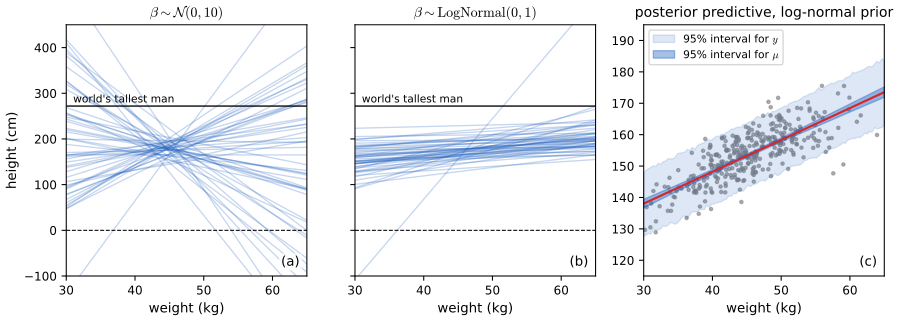
fig_15_1. Reproduces Murphy (2023), Figure 15.1. Download: PDF · SVG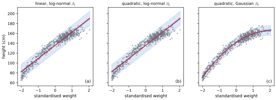
fig_15_2. Reproduces Murphy (2023), Figure 15.2. Download: PDF · SVGFilling the gap 15.7: prior predictive checks, and a Laplace approximation with constrained parameters pp. 601–603
Derivation
The numbers behind Figure 15.1. At a weight 20 kg above the mean, \(\mu=\alpha+20\beta\). With \(\beta\sim\N(0,10^2)\), \(\mu\sim\N(178,20^2+200^2)\), standard deviation 201 cm. Then \(\Pr(\mu>272)=1-\Phi(94/201)=0.32\) and \(\Pr(\mu<0)=\Phi(-178/201)=0.19\): half of the prior lines predict an impossible height at 65 kg. With \(\beta=e^z\), \(z\sim\N(0,1)\): \(\Pr(\mu>272)\approx\Pr(\beta>4.7)=\Pr(z>1.55)=0.06\) with \(\alpha\) fixed at 178 (0.07 once the spread of \(\alpha\) is included) and \(\Pr(\mu<0)=0\), a far more sensible prior. A prior predictive check is nothing more than simulating from \(p(\theta)p(y\given\theta)\) before seeing the data.
Constrained parameters. For \(\beta=e^{z}\) and \(\sigma=e^{s}\) the Laplace approximation (7.4.3) is made for the density of the unconstrained \((\alpha,z,s)\), whose log is \(\log p(y\given\alpha,e^z,e^s)+\log\N(\alpha;178,20^2)+\log\N(z;0,1)+\log\mathrm{Exp}(e^s;\lambda)+s\). The last term is the log-Jacobian of \(\sigma=e^s\); a log-normal prior has no Jacobian term because its density in \(z\) is exactly \(\N(0,1)\). Omitting the Jacobian would move the mode (the mode of a density is not invariant under reparameterisation). The Gaussian approximation on the unconstrained scale is positive after mapping back, so the predictive lines stay increasing. The \(\E[\beta_2\given\mathcal D]\approx0.07\) of the log-normal quadratic (book: 0.08) is the prior's lower boundary at work: the likelihood wants \(\beta_2<0\), the prior forbids it, and the posterior piles up near zero.
15.2.5 Spike and slab prior
p. 603 To select features, make \(w\) sparse. The canonical Bayesian sparsity prior is the spike and slab (Mitchell and Beauchamp 1988): \[ p(w)=\prod_{d=1}^D\big[(1-\pi)\delta(w_d)+\pi\,\mathrm{Unif}(w_d\given-a,a)\big]\tag{15.86} \] (in practice a broad Gaussian slab \(\N(0,\sigma_w^2)\), (15.88)). MAP estimation under this prior is \(\ell_0\) regularisation, (15.87). Unlike the lasso, posterior samples are sparse too, and the posterior mean with a spike-and-slab prior predicts better than the lasso mode (Ewald and Yuan 2009; Scheipl et al. 2009). The price is discrete inference (greedy search or MCMC).
Filling the gap 15.8: spike and slab, the \(\ell_0\) penalty and the posterior over subsets (15.86)–(15.88), (15.101) pp. 603–604, 606
Derivation
The \(\ell_0\) penalty. Introduce indicators \(s_d\sim\mathrm{Ber}(\pi)\), \(\pi=\Pr(w_d\neq0)\), as in the mixture (15.86). A configuration \(s\) with \(\|s\|_0=k\) active coordinates has prior mass \(\pi^k(1-\pi)^{D-k}\), so \(\log p(s)=k\log\pi+(D-k)\log(1-\pi)=-\lambda k+\mathrm{const}\) with \(\lambda=\log\frac{1-\pi}{\pi}\): each extra active feature costs \(\lambda\) nats, positive when \(\pi<1/2\). Hence MAP estimation is \(\min_w[-\log p(y\given X,w)+\lambda\|w\|_0]\). (The book writes \(\lambda=\log\frac{\pi}{1-\pi}\) in (15.87), with \(\pi\) as the spike probability in that line but as the slab probability in (15.86); the sign of \(\lambda\) is correct only with the spike reading. A direct enumeration over all \(2^D\) configurations confirms \(\lambda=\log\frac{1-\pi}{\pi}\) when \(\pi\) multiplies the slab.)
Posterior over subsets. With a Gaussian slab, \(w_s\sim\N(0,\sigma_w^2I)\) on the active set and noise variance \(\sigma_y^2\), integrating the weights (a Gaussian convolution, Chapter 3.4) gives \(y\given s\sim\N(0,C_s)\), \(C_s=\sigma_y^2I+\sigma_w^2X_sX_s^\T\) (15.101), and \(p(s\given y)\propto p(s)\,\N(y\given0,C_s)\). For \(D\) up to about 20 this can be enumerated exactly; otherwise one samples \(s\) by Gibbs or Metropolis. Posterior draws of \(w\) are sparse because \(\Pr(s_d=0\given y)>0\) puts positive probability on the event \(w_d=0\) exactly.
One coefficient. If \(y\given w\sim\N(w,1)\) (an orthonormal design after rotation) and the slab is \(\N(0,s^2)\): \(\Pr(s=1\given y)=\frac{\pi\N(y;0,1+s^2)}{\pi\N(y;0,1+s^2)+(1-\pi)\N(y;0,1)}\) and \(\E[w\given y]=\Pr(s=1\given y)\frac{s^2}{1+s^2}y\). This is the green curve of Figure 15.X1: close to zero for small \(|y|\), close to \(y\) for large.
15.2.6 Laplace prior (Bayesian lasso)
pp. 604–605 MAP estimation with a Laplace prior is the lasso, \(\mathrm{PNLL}(w)=\|Xw-y\|_2^2+\lambda\|w\|_1\) (15.89); see 11.4. The Bayesian lasso (Park and Casella 2008) keeps the posterior: \(p(w_j\given\sigma^2)=\frac{\gamma}{2\sigma}e^{-\gamma|w_j|/\sigma}\) (15.90), conditioned on \(\sigma^2\) to make the posterior unimodal. Writing the Laplace density as a Gaussian scale mixture, \[ \mathrm{Laplace}(w\given0,\gamma)=\int\N(w\given0,\tau^2)\,\Ga\big(\tau^2\given1,\tfrac{\gamma^2}2\big)\,\d\tau^2,\tag{15.91} \] gives the hierarchical model (15.92) and a Gibbs sampler. The group lasso has \(w_g\sim\N(0,\sigma^2\tau_g^2I_{d_g})\) with \(\tau_g^2\sim\Ga(\frac{d_g+1}2,\frac{\gamma^2}2)\) (15.93), (15.94): one variance per group, so small coefficients in a group force the others small. The Gibbs samples are not sparse although the MAP estimate is.
Filling the gap 15.9: the Laplace scale mixture, the group version and the Gibbs conditionals (15.90)–(15.94) pp. 604–605
Derivation
The mixture. Use \(\int_0^\infty t^{-1/2}\exp\{-a/t-bt\}\d t=\sqrt{\pi/b}\,e^{-2\sqrt{ab}}\) (\(a,b>0\)). With \(a=w^2/2\), \(b=\gamma^2/2\) and \(t=\tau^2\): \[ \int\N(w\given0,t)\,\tfrac{\gamma^2}{2}e^{-\gamma^2t/2}\d t=\frac{\gamma^2}{2\sqrt{2\pi}}\int t^{-1/2}e^{-w^2/(2t)-\gamma^2t/2}\d t=\frac{\gamma^2}{2\sqrt{2\pi}}\sqrt{\frac{2\pi}{\gamma^2}}e^{-\gamma|w|}=\frac\gamma2e^{-\gamma|w|}, \] the Laplace density (here \(\Ga(1,r)\) with rate \(r\) is \(re^{-rt}\)); (15.91). Numerical quadrature agrees at several \(w\).
Group version. For \(w_g\in\R^{d}\), \(\int\N(w_g\given0,tI_d)\,\Ga(t\given\frac{d+1}2,\frac{\gamma^2}2)\,\d t\propto\int t^{-d/2}e^{-\|w_g\|^2/(2t)}\,t^{(d+1)/2-1}e^{-\gamma^2t/2}\d t=\int t^{-1/2}e^{-\|w_g\|^2/(2t)-\gamma^2t/2}\d t\propto e^{-\gamma\|w_g\|_2}\): the exponent \(\frac{d+1}2\) is exactly what cancels \(t^{-d/2}\) and reproduces the same integral with \(\|w_g\|\) in place of \(|w|\). The prior is \(\propto\exp(-\gamma\|w_g\|_2)\), the group-lasso penalty (so the shape parameter in (15.94) is \(\frac{d_g+1}2\)).
Gibbs conditionals. With \(w_j\given\sigma^2,\tau_j^2\sim\N(0,\sigma^2\tau_j^2)\) and \(\tau_j^2\sim\Ga(1,\gamma^2/2)\): given \((\tau_j^2)\) and \(\sigma^2\), \(w\) is Gaussian: \(w\sim\N(A^{-1}X^\T y,\sigma^2A^{-1})\) with \(A=X^\T X+\diag(1/\tau_j^2)\) (a ridge posterior with coordinate-specific penalties). The variance \(\tau_j^2\) has full conditional \(\propto(\tau_j^2)^{-1/2}\exp\{-w_j^2/(2\sigma^2\tau_j^2)-\gamma^2\tau_j^2/2\}\); for \(u=1/\tau_j^2\) the density is \(\propto u^{-3/2}\exp\{-\frac{w_j^2}{2\sigma^2}u-\frac{\gamma^2}{2u}\}\), which is the inverse-Gaussian \(u^{-3/2}\exp\{-\lambda u/(2\mu^2)-\lambda/(2u)\}\) with \(\lambda=\gamma^2\), \(\mu^2=\gamma^2\sigma^2/w_j^2\). So \(1/\tau_j^2\sim\mathrm{InvGauss}(\sqrt{\gamma^2\sigma^2/w_j^2},\gamma^2)\), and \(\sigma^2\) (with \(p(\sigma^2)\propto1/\sigma^2\)) is inverse-gamma. A run of this sampler on a one-dimensional problem reproduces the posterior mean found by two-dimensional grid quadrature (0.547 against 0.547).
No exact zeros. The joint posterior has a density with respect to Lebesgue measure, so \(\Pr(w_j=0\given\mathcal D)=0\): every Gibbs draw has all coordinates non-zero, however close the MAP is to a sparse vector.
15.2.7 Horseshoe prior
pp. 605–606 A continuous prior that is both sparse-looking and computationally easy is the horseshoe (Carvalho et al. 2010): \[ w_j\sim\N(0,\gamma_j^2\tau^2),\qquad\gamma_j\sim\mathcal C^+(0,1),\qquad\tau^2\sim\mathcal C^+(0,1),\tag{15.95-15.97} \] with local scales \(\gamma_j\) and a global scale \(\tau\). The Cauchy tails make \(w_j\) either close to 0 or very far from it, emulating the spike and slab without discrete variables.
Filling the gap 15.10: why the horseshoe behaves like a spike and a slab pp. 605–606
Derivation
The shrinkage weight. Take \(y_j\given w_j\sim\N(w_j,1)\) (one coefficient, unit noise) and \(w_j\given\gamma_j,\tau\sim\N(0,\gamma_j^2\tau^2)\). The posterior given \(\gamma_j\) is \(\N((1-\kappa_j)y_j,1-\kappa_j)\) with \(\kappa_j=\frac1{1+\tau^2\gamma_j^2}\): the posterior mean is the data shrunk by the factor \(\kappa_j\in(0,1)\) (Gaussian conjugacy). A Gaussian prior has a fixed \(\kappa\); a Laplace prior has a scale mixture of \(\kappa\) values with little mass near 1; the horseshoe's \(\kappa\) has a U-shaped density. For \(\tau=1\) and \(\gamma\sim\mathcal C^+(0,1)\), \(p(\gamma)=\frac2{\pi(1+\gamma^2)}\); under \(\kappa=1/(1+\gamma^2)\), \(\gamma=\sqrt{(1-\kappa)/\kappa}\), \(|\d\gamma/\d\kappa|=\frac12\kappa^{-3/2}(1-\kappa)^{-1/2}\) and \(1+\gamma^2=1/\kappa\), so \[ p(\kappa)=\frac2\pi\kappa\cdot\frac12\kappa^{-3/2}(1-\kappa)^{-1/2}=\frac1\pi\kappa^{-1/2}(1-\kappa)^{-1/2}, \] the \(\mathrm{Beta}(\frac12,\frac12)\) density (Figure 15.X1c). Half the prior mass is on \(\kappa>1/2\) (near-total shrinkage, a "spike") and half on \(\kappa<1/2\), with infinite density at \(\kappa=0\) (no shrinkage of large signals, a "slab"). A Kolmogorov-Smirnov test of simulated \(\kappa\) against \(\mathrm{Beta}(\frac12,\frac12)\) agrees.
Marginal prior. \(p(w)=\int\N(w\given0,\gamma^2\tau^2)p(\gamma)\d\gamma\). Near zero the integrand over \(\gamma\in(|w|/\tau,\tau)\) is of the order \(1/\gamma\), so \(p(w)\gtrsim c\log(1/|w|)\): an unbounded spike at 0. In the tails, restrict to \(\gamma\in[|w|,2|w|]\) (take \(\tau=1\)): \(\N(w\given0,\gamma^2)\ge(2\pi)^{-1/2}(2|w|)^{-1}e^{-1/2}\) and \(p(\gamma)\ge\frac2{\pi(1+4w^2)}\), so \(p(w)\ge c'\,w^{-2}\) for large \(|w|\): polynomial (Cauchy-like) tails, against exponential tails for the Laplace and Gaussian priors. Hence large coefficients are shrunk very little (Figure 15.X1b, red curve approaches the diagonal), while small ones are shrunk almost to zero. The numerical marginal confirms \(p(w)w^2\) stays bounded away from 0 and \(\infty\).
Inference. With the representation \(\gamma^2\given\nu\sim\IG(\frac12,\frac1\nu)\), \(\nu\sim\IG(\frac12,1)\) (a half-Cauchy as an inverse-gamma mixture, Makalic and Schmidt 2016) all full conditionals of \(w,\gamma_j^2,\tau^2,\sigma^2\) and the auxiliary variables are Gaussian or inverse-gamma, so a Gibbs sampler (horseshoe_gibbs) needs no tuning. On a sparse regression its posterior mean is closer to the truth than least squares (error 0.24 against 0.53 in a run of the checks). Samples are not exactly sparse but concentrate near zero for irrelevant coefficients.
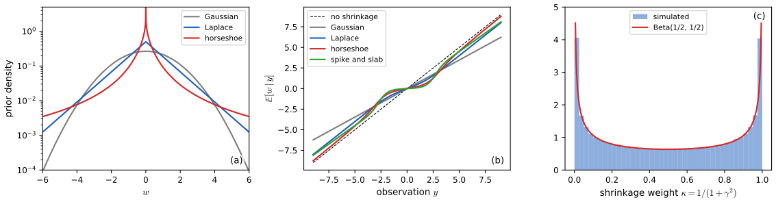
fig_15_X1. Download: PDF · SVGSee also: 11.4.2 why \(\ell_1\) regularisation yields sparse solutions.
15.2.8 Automatic relevancy determination
pp. 606–608 A different route to sparsity: keep a Gaussian prior \(w_j\sim\N(0,1/\alpha_j)\) but choose all precisions by empirical Bayes, \(\hat\alpha=\argmax_\alpha p(y\given X,\alpha)\). Remarkably the estimate is sparse. The method is sparse Bayesian learning (Tipping 2001), automatic relevancy determination (ARD, MacKay 1995; Neal 1996) or "NUV" estimation. With \(\beta=1/\sigma^2\) and \(A=\diag(\alpha)\) the marginal likelihood is \[ p(y\given X,\alpha,\beta)=\int\N(y\given Xw,\beta^{-1}I)\N(w\given0,A^{-1})\,\d w=\N(y\given0,C_\alpha),\quad C_\alpha=\beta^{-1}I_N+XA^{-1}X^\T\tag{15.98-15.100} \] and the objective is \(\ell(\alpha,\beta)=\log|C_\alpha|+y^\T C_\alpha^{-1}y\) (15.102), minus twice the log marginal likelihood up to the constant \(N\log2\pi\). It differs from (15.101) of the spike-and-slab only in that the binary indicators have been relaxed to continuous precisions, and although it is not convex it has far fewer local optima than \(\ell_0\) regularisation (Wipf and Nagarajan 2010).
Filling the gap 15.11: the ARD objective, its stationarity condition, and the EM and MacKay updates (15.98)–(15.103) pp. 606–608
Derivation
The marginal. \(y=Xw+\varepsilon\) with \(w\sim\N(0,A^{-1})\) and independent \(\varepsilon\sim\N(0,\beta^{-1}I)\) is a linear function of Gaussians, hence Gaussian with mean 0 and covariance \(XA^{-1}X^\T+\beta^{-1}I=C_\alpha\) (15.99), (15.100).
A form with the posterior. Let \(\Sigma=(A+\beta X^\T X)^{-1}\), \(\mu=\beta\Sigma X^\T y\) (the posterior of \(w\); Bayes' rule for Gaussians). The matrix determinant lemma gives \(|C_\alpha|=\beta^{-N}|A|^{-1}|A+\beta X^\T X|=\beta^{-N}|A|^{-1}|\Sigma|^{-1}\), and Woodbury gives \(y^\T C_\alpha^{-1}y=\min_w\{\beta\|y-Xw\|^2+w^\T Aw\}\), attained at \(w=\mu\) (the quadratic form of a ridge problem equals the minimum value of its penalised objective). Hence \[ \ell(\alpha,\beta)=-N\log\beta-\sum_j\log\alpha_j+\log|A+\beta X^\T X|+\beta\|y-X\mu\|^2+\mu^\T A\mu. \] Stationarity. Differentiate with respect to \(\alpha_j\). \(\mu\) minimises the last two terms, so by the envelope theorem its dependence on \(\alpha_j\) drops out and only the explicit \(\mu_j^2\) remains; \(\partial\log|A+\beta X^\T X|/\partial\alpha_j=\Sigma_{jj}\). So \(-1/\alpha_j+\Sigma_{jj}+\mu_j^2=0\), i.e. \[ \alpha_j\,(\mu_j^2+\Sigma_{jj})=1 .\] Similarly \(\partial\ell/\partial\beta=-N/\beta+\Tr(\Sigma X^\T X)+\|y-X\mu\|^2=0\).
Two fixed-point iterations of one equation. (i) EM. Treat \(w\) as latent. The expected complete-data log likelihood is \(\E[\log p(y\given w,\beta)+\log p(w\given\alpha)]\); maximising over \(\alpha_j\) gives \(\alpha_j=1/\E[w_j^2]=1/(\mu_j^2+\Sigma_{jj})\), and over \(\beta\) gives \(\beta^{-1}=\frac1N(\|y-X\mu\|^2+\Tr(X\Sigma X^\T))\). These are just the stationarity equations solved for \(\alpha_j\) and \(\beta\); EM theory guarantees the marginal likelihood never decreases (confirmed numerically). (ii) MacKay. Since \(\Sigma(A+\beta X^\T X)=I\), \(\beta\Sigma X^\T X=I-\Sigma A\), so \(\Tr(\beta\Sigma X^\T X)=\sum_j\gamma_j\) with \(\gamma_j=1-\alpha_j\Sigma_{jj}\in(0,1)\), the "number of well-determined parameters". Rearranging the same stationarity equation as \(\alpha_j\mu_j^2=1-\alpha_j\Sigma_{jj}\) gives \(\alpha_j=\gamma_j/\mu_j^2\), and the \(\beta\) equation becomes \(\beta=(N-\sum_j\gamma_j)/\|y-X\mu\|^2\). Both iterations share their fixed points; MacKay's usually moves faster (Figure 15.X2f). See also ml 3.5.3. A third view (15.103): put \(\alpha_d\sim\Ga(a,b)\) and use variational Bayes with \(q(w,\alpha)=q(w)q(\alpha)\); ARD is the version where \(q(\alpha)\) is a point mass.
Filling the gap 15.12: why ARD prunes irrelevant features (Tipping and Faul) p. 607
Derivation
The book gives a geometric argument (Figure 15.4); here is the exact condition. Fix all hyperparameters but \(\alpha_j\) and write \(C=C_{-j}+\alpha_j^{-1}\varphi_j\varphi_j^\T\), where \(\varphi_j\) is column \(j\) of \(X\) and \(C_{-j}\) is the covariance without feature \(j\). Define the sparsity factor \(s_j=\varphi_j^\T C_{-j}^{-1}\varphi_j\) and the quality factor \(q_j=\varphi_j^\T C_{-j}^{-1}y\). By the determinant lemma \(|C|=|C_{-j}|(1+s_j/\alpha_j)\) and by Sherman-Morrison \(y^\T C^{-1}y=y^\T C_{-j}^{-1}y-\frac{q_j^2}{\alpha_j+s_j}\). So, up to terms not involving \(\alpha_j\), \[ L(\alpha_j)=\log p(y\given\alpha_j)=\tfrac12\Big[\log\alpha_j-\log(\alpha_j+s_j)+\frac{q_j^2}{\alpha_j+s_j}\Big]. \] Its derivative is \(L'(\alpha_j)=\frac12\big[\frac1{\alpha_j}-\frac1{\alpha_j+s_j}-\frac{q_j^2}{(\alpha_j+s_j)^2}\big]=\frac{s_j(\alpha_j+s_j)-q_j^2\alpha_j}{2\alpha_j(\alpha_j+s_j)^2}\). The numerator is \(s_j^2+(s_j-q_j^2)\alpha_j\). Case \(q_j^2>s_j\): it has a unique positive root \(\alpha_j=s_j^2/(q_j^2-s_j)\), positive before it and negative after: a maximum, so the feature is retained. Case \(q_j^2\le s_j\): the numerator is positive for every \(\alpha_j>0\), so \(L\) increases without bound in \(\alpha_j\) and the maximiser is \(\alpha_j=\infty\): feature \(j\) is pruned (its weight is 0). Large \(q_j^2\) means the feature explains \(y\) beyond what the other features already do; \(s_j\) measures how much the feature's own noise-like variability is penalised. In the one-feature picture of the book, an irrelevant \(x\) (nearly orthogonal to \(y\)) has \(q^2\approx0\le s\), so the evidence is maximised at \(\alpha=\infty\) (Figure 15.X2c, red). The formula for the finite maximiser matches a numerical one-dimensional maximisation to 3 digits in the fitted example (\(q^2=49.6\), \(s=23.5\), \(\alpha=21\)).
Filling the gap 15.13: the Gamma mixture of Gaussians is a Student (15.104) pp. 607–608
Derivation
For one weight, \(\int_0^\infty\N(w\given0,1/\alpha)\Ga(\alpha\given a,b)\d\alpha=\frac{b^a}{\Gamma(a)\sqrt{2\pi}}\int\alpha^{a-1/2}e^{-\alpha(b+w^2/2)}\d\alpha=\frac{b^a\Gamma(a+\frac12)}{\Gamma(a)\sqrt{2\pi}}\Big(b+\frac{w^2}2\Big)^{-(a+1/2)}\propto\Big(1+\frac{w^2}{2b}\Big)^{-(a+1/2)}\), a Student with \(\nu=2a\) degrees of freedom and squared scale \(b/a\). With small \(a\) and \(b\) it has a high narrow peak at 0 and heavy tails, so a prior of independent Student weights is sparsity-inducing, which is why variational ARD (and the relevance vector machine below) gives sparse means. Marginalising the vector \(w\) with a shared Gamma precision per coordinate gives a product of such Students; the non-diagonal covariance mentioned in the book appears for the full posterior \(q(w)\) after the likelihood couples the coordinates.
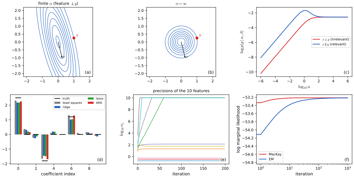
fig_15_X2. Reproduces and extends Murphy (2023), Figure 15.4. Download: PDF · SVGRelevance vector machines
p. 608 Replacing \(x\) by the kernel features \(\phi(x)=[K(x,x_1),\dots,K(x,x_N)]\) gives a model with \(N\) parameters, but ARD prunes most of them, leaving a few relevance vectors (Tipping 2001; Tipping and Faul 2003). See ml 7.2. Applying ARD to the kernel basis is exactly the feature-selection problem above with \(D=N\) columns.
15.2.9 Multivariate linear regression
pp. 608–610 For \(N_y\) outputs, \(Y=WX+E\) with \(W\in\R^{N_y\times N_x}\), \(X\in\R^{N_x\times N}\) and columns \(e_n\sim\N(0,\Sigma)\) (15.105). The likelihood is a matrix normal (15.106)–(15.108), the conjugate prior is the matrix-normal inverse-Wishart \(W\given\Sigma\sim\mathrm{MN}(M_0,\Sigma,V_0)\), \(\Sigma\sim\mathrm{IW}(\nu_0,\Psi_0)\) (15.109)–(15.111), and the posterior is again MNIW: \[ M_1=S_{yx}S_{xx}^{-1},\ V_1=S_{xx},\ \nu_1=N+\nu_0,\ \Psi_1=\Psi_0+S_{y|x}\ (15.122\text{–}15.125),\quad\hat W=M_1,\ \ \hat\Sigma=\frac{\Psi_1}{\nu_1+N_y+N_x+1}\ (15.126, 15.127), \] with \(S_{xx}=XX^\T+V_0\), \(S_{yx}=YX^\T+M_0V_0\), \(S_{yy}=YY^\T+M_0V_0M_0^\T\), \(S_{y|x}=S_{yy}-S_{yx}S_{xx}^{-1}S_{yx}^\T\) (15.118), (15.119). (This section of the book is by Xinglong Li.)
Filling the gap 15.14: the matrix-normal inverse-Wishart posterior and its MAP estimate (15.112)–(15.127) pp. 608–610
Derivation
Here \(W\given\Sigma\) has density \(\propto|\Sigma|^{-N_x/2}\exp\{-\frac12\Tr[\Sigma^{-1}(W-M_0)V_0(W-M_0)^\T]\}\) (\(V_0\) acts as a precision on the input side), \(\Sigma\) has the inverse-Wishart density \(\propto|\Sigma|^{-(\nu_0+N_y+1)/2}e^{-\frac12\Tr\Sigma^{-1}\Psi_0}\), and the likelihood is \(\propto|\Sigma|^{-N/2}\exp\{-\frac12\Tr[\Sigma^{-1}(Y-WX)(Y-WX)^\T]\}\). The joint is therefore \(\propto|\Sigma|^{-(\nu_0+N+N_y+N_x+1)/2}\exp\{-\frac12\Tr\Sigma^{-1}\Omega\}\) with \(\Omega=\Psi_0+(Y-WX)(Y-WX)^\T+(W-M_0)V_0(W-M_0)^\T\) (15.112), (15.113).
Completing the square. Expand and collect: \((Y-WX)(Y-WX)^\T+(W-M_0)V_0(W-M_0)^\T=WS_{xx}W^\T-WS_{yx}^\T-S_{yx}W^\T+S_{yy}\) with the \(S\) matrices above. Since \(S_{xx}\succ0\), \[ WS_{xx}W^\T-WS_{yx}^\T-S_{yx}W^\T+S_{yy}=(W-S_{yx}S_{xx}^{-1})S_{xx}(W-S_{yx}S_{xx}^{-1})^\T+S_{yy}-S_{yx}S_{xx}^{-1}S_{yx}^\T, \] which is the content of (15.114)–(15.117). So, with \(M_1=S_{yx}S_{xx}^{-1}\), \(V_1=S_{xx}\), \(\Psi_1=\Psi_0+S_{y|x}\), \(\nu_1=\nu_0+N\): \[ p(W,\Sigma\given X,Y)\propto|\Sigma|^{-(\nu_1+N_y+N_x+1)/2}\exp\{-\tfrac12\Tr\Sigma^{-1}[\Psi_1+(W-M_1)V_1(W-M_1)^\T]\}. \] Given \(\Sigma\), \(W\) is matrix normal with mean \(M_1\) and column precision \(V_1\) (15.120). Integrating \(W\) gives \(|\Sigma|^{N_x/2}|V_1|^{-N_y/2}\), which cancels the \(|\Sigma|^{-N_x/2}\) of the matrix-normal factor and leaves \(|\Sigma|^{-(\nu_1+N_y+1)/2}e^{-\frac12\Tr\Sigma^{-1}\Psi_1}\): \(\Sigma\given\mathcal D\sim\mathrm{IW}(\nu_1,\Psi_1)\). The prior thus conjugates, and the update counts \(N\) observations in the degrees of freedom. A direct numerical comparison of "prior times likelihood" with the formula above at random \((W,\Sigma)\) gives a constant difference.
MAP. The joint density is maximised in \(W\) at \(W=M_1\) for every \(\Sigma\) (the quadratic form is nonnegative), so \(\hat W=M_1\). At \(W=M_1\), \(\log p=-\frac c2\log|\Sigma|-\frac12\Tr\Sigma^{-1}\Psi_1\) with \(c=\nu_1+N_y+N_x+1\), whose gradient in \(\Sigma\) is \(-\frac c2\Sigma^{-1}+\frac12\Sigma^{-1}\Psi_1\Sigma^{-1}\), zero at \(\hat\Sigma=\Psi_1/c\); this is a maximum because \(\Tr\Sigma^{-1}\Psi_1\) is convex and \(\log|\Sigma|\) concave in the right directions (checked numerically). For \(N_y=1\) the whole result reduces to the NIG posterior of gap 15.4 with \(\hat a=\nu_1/2\).
15.3 Logistic regression
p. 610 Logistic regression maps \(x\in\R^D\) to a distribution over \(C\) classes. The model, its maximum likelihood fit and MAP estimation are in the introductory volume, Chapter 10; this chapter adds priors, posteriors and predictive approximations.
15.3.1 Binary logistic regression
pp. 610–611 \(p(y\given x;\theta)=\mathrm{Ber}(y\given\sigma(w^\T x+b))\) (15.128). With logits \(\eta_n\) and \(\mu_n=\sigma(\eta_n)\) the log likelihood is the negative cross entropy, which simplifies to \(\sum_ny_n\eta_n-\sum_n\log(1+e^{\eta_n})\) (15.130)–(15.134): one line, using \(\mu_n=e^{\eta_n}/(1+e^{\eta_n})\) and \(1-\mu_n=1/(1+e^{\eta_n})\). In code, \(\log(1+e^a)\) is computed stably with logaddexp(0, a) (or log1p(exp(a)) for moderate \(a\)).
15.3.2 Multinomial logistic regression
p. 611 \(p(y\given x;\theta)=\mathrm{Cat}(y\given\softmax(Wx+b))\) (15.135), (15.136), with log likelihood \(\sum_n\sum_cy_{nc}\log\mu_{nc}\) (15.137), the negative cross entropy for one-hot labels. See 10.3.
15.3.3 Dealing with class imbalance and the long tail
p. 612 Maximum likelihood minimises a bound on the 0-1 loss, which is dominated by frequent classes. The balanced error rate \(\mathrm{BER}(f)=\frac1C\sum_y\Pr_{x\sim p^*(\cdot|y)}[y\notin\argmax_{y'}f_{y'}(x)]\) (15.138) weights classes equally; its minimiser satisfies \(\argmax_yf^*_y(x)=\argmax_yp^*(x\given y)\) (15.139). Logit adjustment (Menon et al. 2021) achieves this: train as usual, then predict \[ \hat f(x)=\argmax_y\ f_y(x)-\tau\log\pi_y\tag{15.141} \] with \(\pi_y\) the empirical label prior and \(\tau=1\) the theoretically justified value (15.140); alternatively train with the logit-adjusted softmax loss \(-\log\frac{e^{f_y(x)+\tau\log\pi_y}}{\sum_{y'}e^{f_{y'}(x)+\tau\log\pi_{y'}}}\) (15.142). One can combine either with a prior on the parameters (a "generalised Bayes" use of a non-likelihood loss, 14.1.3).
Filling the gap 15.15: the balanced-error optimal rule and why logit adjustment attains it (15.138)–(15.142) p. 612
Derivation
Optimal rule. For a classifier \(f\) with decision \(\hat y(x)=\argmax_yf_y(x)\), \(\mathrm{BER}=1-\frac1C\sum_y\Pr[\hat y(x)=y\given y]=1-\frac1C\int\sum_y1[\hat y(x)=y]\,p^*(x\given y)\,\d x\). The inner sum equals \(p^*(x\given\hat y(x))\) at each \(x\); the integral is largest when \(\hat y(x)\) maximises \(p^*(x\given y)\) at every \(x\), which is (15.139). Equivalently \(\hat y=\argmax_yp^*_{\rm bal}(y\given x)\), where \(p^*_{\rm bal}(y\given x)=\frac{p^*(x|y)/C}{\sum_{y'}p^*(x|y')/C}\) is the posterior under a uniform class prior.
Post-hoc adjustment. If the logits are calibrated in the sense \(f_y(x)=\log p^*(y\given x)+c(x)\) (a class-independent shift \(c\) does not matter for softmax), Bayes' rule gives \(\log p^*(x\given y)=\log p^*(y\given x)-\log\pi_y+\log p^*(x)=f_y(x)-\log\pi_y+\mathrm{const}(x)\), so \(\argmax_yp^*(x\given y)=\argmax_y[f_y(x)-\log\pi_y]\): (15.140), (15.141) with \(\tau=1\).
Loss-based adjustment. Minimising the softmax cross-entropy over all functions makes \(\softmax(g)=p^*(y\given x)\) (the proper-scoring property, 14.2.1). Under (15.142) the model whose softmax is trained is \(g_y=f_y+\tau\log\pi_y\); at the optimum \(g_y=\log p^*(y\given x)+c\), so \(f_y=\log p^*(y\given x)-\tau\log\pi_y+c\), and for \(\tau=1\), \(f_y=\log p^*(x\given y)+c'\): the learned scores already rank classes by the likelihood, and plain \(\argmax f\) at test time is balanced-error optimal. A simulation with two Gaussian classes in the ratio 10:1 shows the balanced error dropping from 0.42 to 0.25, equal to that of the true likelihood rule.
15.3.4 Parameter priors
pp. 612–613 Gaussian priors are standard, with mean 0 for symmetry. But the variance cannot be taken large "to approximate a uniform prior". Consider only an offset: \(y\sim\mathrm{Ber}(\sigma(\alpha))\), \(\alpha\sim\N(0,\omega)\) (15.143), (15.144). For \(\omega=10\) the implied prior on \(\sigma(\alpha)\) is U-shaped with most mass near 0 and 1, for \(\omega=1.5\) it is nearly flat (Figure 15.5a). With features the problem grows: for random binary vectors \(x_{nd}\sim\mathrm{Ber}(0.8)\) and \(\beta\sim\N(0,1.5I)\) the induced distribution of the fraction of ones, flat for one feature, becomes extreme as \(D\) grows (Figure 15.5b). Remedies: standardise the inputs, scale the prior standard deviation by \(1/\sqrt D\), or use heavier-tailed priors (Cauchy, Student; Gelman et al. 2008).
Filling the gap 15.16: the prior on the probability scale, and why the logit variance grows with \(D\) pp. 612–613
Derivation
Change of variables. Let \(s=\sigma(\alpha)\), so \(\alpha=\logit s=\log\frac s{1-s}\) and \(\d\alpha/\d s=\frac1{s(1-s)}\). Then \[ p_S(s)=\N(\logit s\given0,\omega)\cdot\frac1{s(1-s)},\qquad s\in(0,1). \] Since \(1/(s(1-s))=4\cosh^2(z/2)\) for \(z=\logit s\), the density in \(z\) is proportional to \(e^{-z^2/(2\omega)}\cosh^2(z/2)\). Near \(z=0\) it is \(1+z^2(\frac14-\frac1{2\omega})+O(z^4)\), so \(s=\frac12\) is a local minimum (a U shape) exactly when \(\omega>2\) and a maximum when \(\omega<2\); the density does tend to 0 at the very ends (the Gaussian beats \(e^{|z|}\)), but for large \(\omega\) its peaks sit near \(|z|=\omega\), i.e. very close to 0 and 1. The mass beyond \((0.05,0.95)\) is \(\Pr(|\alpha|>\log19)=2\Phi(-\log19/\sqrt\omega)=2\Phi(-2.944/\sqrt\omega)\): 0.352 for \(\omega=10\) and 0.016 for \(\omega=1.5\) (confirmed by simulation). The density is exactly uniform when \(\alpha\) has the standard logistic distribution (variance \(\pi^2/3=3.29\)): then \(s=F(\alpha)\) with \(F=\sigma\) the logistic cdf, uniform by the probability integral transform.
Several features. For one data point with \(x\) of independent \(\mathrm{Ber}(p)\) coordinates and \(\beta\sim\N(0,s_\beta^2I_D)\), the logit \(\eta=\beta^\T x\) has \(\E[\eta^2]=s_\beta^2\E\|x\|^2=s_\beta^2Dp\): the variance grows linearly in \(D\). More relevant for the fraction of ones is the part of the logit common to all inputs, \(\bar\eta(\beta)=\E_x[\eta]=p\sum_d\beta_d\sim\N(0,p^2s_\beta^2D)\); for \(s_\beta=1.5\), \(p=0.8\) and \(D=15\) its standard deviation is \(\sqrt{0.64\cdot2.25\cdot15}=4.6\) and the probability of an extreme dataset (fraction of ones outside \((0.1,0.9)\)) is large (about 0.4 in simulation, against 0.01 for \(D=1\)). Taking \(s_\beta\propto1/\sqrt D\) keeps \(p^2s_\beta^2D\) fixed as \(D\) grows, which is the rule given in the text.
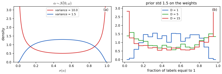
fig_15_5. Reproduces Murphy (2023), Figure 15.5. Download: PDF · SVG15.3.5 Laplace approximation to the posterior
pp. 613–615 There is no conjugate prior for logistic regression. The Laplace approximation (7.4.3) takes \(p(w\given\mathcal D)\approx\N(w\given\hat w,H^{-1})\) with \(\hat w=\argmin[-\log p(w,\mathcal D)]\) and \(H=-\nabla^2\log p(w,\mathcal D)\vert_{\hat w}\) (15.145). In Figure 15.6 the data are linearly separable (panel a shows four separating lines through the origin with weights \((3,1),(4,2),(5,3),(7,3)\), of increasing norm 3.16, 4.47, 5.83, 7.62). The likelihood (b) increases along a ray to infinity, so the MLE does not exist; a spherical prior \(\N(0,\sigma^2I)\) with \(\sigma^2=100\) gives a finite MAP (c); its Laplace approximation (d) gets the mode right but distorts the shape (long axis: the weight norm; short axis: the boundary orientation).
Filling the gap 15.17: the Hessian, separable data and the existence of the MAP estimate pp. 613–615
Derivation
Hessian. For \(p(y\given x,w)=\mathrm{Ber}(\sigma(w^\T x))\) and the prior \(\N(0,\sigma_0^2I)\), the negative log posterior is \(\sum_n[\log(1+e^{\eta_n})-y_n\eta_n]+\|w\|^2/(2\sigma_0^2)+\mathrm{const}\) with gradient \(X^\T(\mu-y)+w/\sigma_0^2\) and Hessian \[ H=X^\T SX+\sigma_0^{-2}I,\qquad S=\diag(\mu_n(1-\mu_n)),\] which is positive definite for every \(w\) (the data term is positive semidefinite by gap 15.3 and the prior term is \(\sigma_0^{-2}I\)). So the objective is strictly convex and coercive (it is at least \(\|w\|^2/(2\sigma_0^2)\) minus a linear term), hence has exactly one minimiser, found by Newton's method.
Separable data. Let \(\tilde y_n=2y_n-1\) and suppose \(\tilde y_nw_*^\T x_n>0\) for all \(n\) (separability). Along the ray \(tw_*\), the NLL is \(\sum_n\log(1+e^{-t\tilde y_nw_*^\T x_n})\), strictly decreasing in \(t\) and tending to 0 as \(t\to\infty\); no finite \(w\) attains the infimum, so the MLE does not exist (it is at infinity along a separating direction, as the contours of Figure 15.6b show). With the prior the penalty \(t^2\|w_*\|^2/(2\sigma_0^2)\) stops the escape. Let \(m\) be the smallest margin \(\tilde y_nw_*^\T x_n\) (with \(\|w_*\|=1\)); for large \(t\) the data term is about \(e^{-tm}\), and the stationarity condition \(me^{-tm}\approx t/\sigma_0^2\) gives \(t\approx\frac1m\log(m\sigma_0^2/t)\): the MAP norm grows only logarithmically in the prior variance (numerically 1.7, 3.1, 4.8, 6.8, 9.0 for \(\sigma_0^2=1,10,10^2,10^3,10^4\)).
The Laplace approximation. Its covariance \(H^{-1}\) is the inverse of the matrix above evaluated at the MAP: the prior variance enters twice, through the mode and through \(H\). A Gaussian cannot represent the skewed, curved posterior of Figure 15.6c, and the Laplace log-evidence \(\log p(w_{\rm map},\mathcal D)+\frac D2\log2\pi-\frac12\log|H|\) is accurate here only to a few hundredths (see Figure 15.X3).
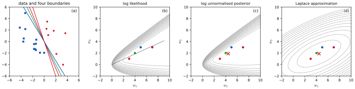
fig_15_6. Reproduces Murphy (2023), Figure 15.6. Download: PDF · SVG15.3.6 Approximating the posterior predictive distribution
pp. 615–617 The predictive is \(p(y\given x,\mathcal D)=\int p(y\given x,w)p(w\given\mathcal D)\d w\) (15.146). Monte Carlo: \(p(y=1\given x,\mathcal D)\approx\frac1S\sum_s\sigma(w_s^\T x)\) with posterior draws (15.147). Deterministic: if \(p(w\given\mathcal D)=\N(\mu,\Sigma)\) the logit \(f_*=\mu^\T x_*\) is Gaussian with variance \(x_*^\T\Sigma x_*\) (15.148), and replacing the sigmoid by a probit gives the closed form \[ p(y_*=1\given x_*)\approx\int\Phi(\lambda f_*)\N(f_*\given\mu_*,\sigma_*^2)\d f_*\ \to\ \sigma\!\Big(\frac{\mu_*}{\sqrt{1+\pi\sigma_*^2/8}}\Big)\tag{15.149} \] (the probit approximation, MacKay/Spiegelhalter-Lauritzen), and for \(C\) classes \(\softmax_c\{\mu_{*,c}/\sqrt{1+\frac\pi8\Sigma_{*,cc}}\}\) (15.150, Gibbs 1997; it ignores logit correlations). Plugging in \(\hat w_{\rm map}\) gives no uncertainty about the boundary (Figure 15.7a); sampled boundaries fan out away from the data (b); averaging gives moderated probabilities (c); the probit approximation is almost identical (d).
Filling the gap 15.18: the probit approximation of the logistic predictive (15.148)–(15.150) pp. 615–616
Derivation
Predictive logit. A linear function of a Gaussian vector is Gaussian: \(w\sim\N(\mu,\Sigma)\Rightarrow f_*=w^\T x_*\sim\N(\mu^\T x_*,x_*^\T\Sigma x_*)\) (15.148).
Step 1: \(\sigma(a)\approx\Phi(\lambda a)\). Match the slope at \(0\): \(\sigma'(0)=\frac14\), \(\frac{\d}{\d a}\Phi(\lambda a)\vert_0=\lambda\phi(0)=\lambda/\sqrt{2\pi}\), so \(\lambda=\sqrt{2\pi}/4\), \(\lambda^2=\pi/8\) (Figure 15.11). The approximation has maximal absolute error 0.018 over the real line.
Step 2: an exact Gaussian integral. If \(f\sim\N(\mu,s^2)\) and \(\varepsilon\sim\N(0,1)\) is independent, then \(\Phi(\lambda f)=\Pr(\varepsilon\le\lambda f\given f)\), so \(\E[\Phi(\lambda f)]=\Pr(\varepsilon-\lambda f\le0)\). The variable \(\varepsilon-\lambda f\) is Gaussian with mean \(-\lambda\mu\) and variance \(1+\lambda^2s^2\), whence \[ \int\Phi(\lambda f)\N(f\given\mu,s^2)\d f=\Phi\Big(\frac{\lambda\mu}{\sqrt{1+\lambda^2s^2}}\Big). \] Step 3: back to the sigmoid. Writing \(\Phi(\lambda\cdot z)\approx\sigma(z)\) with \(z=\mu/\sqrt{1+\lambda^2s^2}=\mu/\sqrt{1+\pi s^2/8}\) gives (15.149). The multiclass rule (15.150) applies the same rule to each logit separately, which treats the logits as independent. The effect is to moderate the probability: \(\sigma\) is evaluated at a point closer to 0 than \(\mu\), more so when the logit uncertainty \(s^2\) is large. On the example of Figure 15.7 the largest difference from a 2000-sample Monte Carlo average is 0.019 over the plane (mean 0.006); at the test point \((2,-1.5)\) they differ by 0.01.
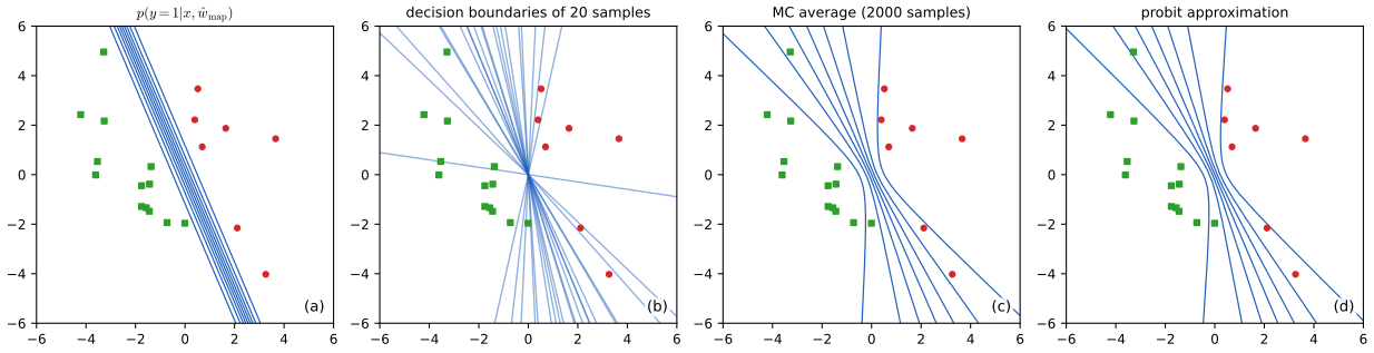
fig_15_7. Reproduces Murphy (2023), Figure 15.7. Download: PDF · SVG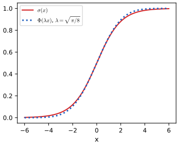
fig_15_11. Reproduces Murphy (2023), Figure 15.11. Download: PDF · SVG15.3.7 MCMC inference
pp. 617–618 MCMC, the "gold standard", returns correlated posterior draws \(\theta_s\) and the empirical approximation (15.151); plug them into (15.147). HMC (12.5) uses \(\nabla_\theta\log p(\mathcal D,\theta)\). For two iris features (sepal length and width) and two classes the decision boundary \(\{x:\sigma(b+w_1x_1+w_2x_2)=0.5\}\) is the line \[ x_2^*=-\frac b{w_2}-\frac{w_1}{w_2}x_1^*\tag{15.152} \] and each posterior draw gives a line; the pointwise mean and 2.5%, 97.5% quantiles of these lines are the posterior mean boundary and its credible band (Figure 15.8a). Making the classes unbalanced (5 against 45 examples) widens the band and shifts the mean boundary towards the class with less data (Figure 15.8b), as in linear discriminant analysis, where raising a class prior enlarges that class's region (introductory volume, Chapter 9).
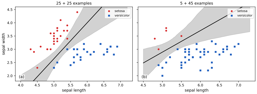
fig_15_8 (sampler hmc, acceptance 0.86 and 0.91, no divergences). Reproduces Murphy (2023), Figure 15.8. Download: PDF · SVG15.3.8 Other approximate inference methods
p. 618 Variational inference turns inference into maximising the ELBO over a family \(q(w;\psi)\) (Chapter 10): by stochastic gradients, by conditionally conjugate VI, or by a local method that lower-bounds the logistic function by a quadratic (the supplement, next). In the online setting assumed density filtering gives a recursive Gaussian posterior (online logistic ADF demo, Chapter 8.6; expectation propagation: demo).
S15.1 Variational inference for logistic regression (supplement)
Supplement pp. 161–166 With prior \(p(w)=\N(w\given\mu_0,V_0)\), a Gaussian-like lower bound on each likelihood factor makes the product conjugate to the prior. For one observation, \(p(y_n\given x_n,w)=e^{\eta_ny_n}\sigma(-\eta_n)\) (S15.1)–(S15.3) (the printed exponents in the draft carry sign slips: see Notes on the book). The Jaakkola-Jordan (JJ) bound is \[ \sigma(\eta)\ \ge\ \sigma(\psi)\exp\!\big[(\eta-\psi)/2-\lambda(\psi)(\eta^2-\psi^2)\big],\qquad\lambda(\psi)=\tfrac1{4\psi}\tanh\tfrac\psi2=\tfrac1{2\psi}\big(\sigma(\psi)-\tfrac12\big)\tag{S15.4, S15.5} \] with one variational parameter \(\psi_n\) per example, tight at \(\eta=\pm\psi_n\). Then \(\log p(y\given X,w)+\log p(w)\) is bounded by a quadratic in \(w\) (S15.7), (S15.8), so \[ q(w\given\psi)=\N(w\given\mu_N,V_N),\quad V_N^{-1}=V_0^{-1}+2\sum_n\lambda(\psi_n)x_nx_n^\T,\quad\mu_N=V_N\Big(V_0^{-1}\mu_0+\sum_n(y_n-\tfrac12)x_n\Big)\tag{S15.9-S15.11} \] and maximising the bound on the evidence, \(\log p(y\given X)\ge\mathcal L(\psi)\) (S15.12), (S15.14), gives the update \((\psi_n^{\rm new})^2=x_n^\T(V_N+\mu_N\mu_N^\T)x_n\) (S15.15). It is more flexible than the Laplace approximation because \(\psi\) tunes the curvature of the covariance.
Filling the gap 15.19: the Jaakkola-Jordan bound and the \(\psi\) update (S15.4)–(S15.15) Supplement pp. 161–163
Derivation
The bound. Write \(\log\sigma(\eta)=\eta/2-g(\eta)\) with \(g(\eta)=\log(e^{\eta/2}+e^{-\eta/2})\), an even function. Set \(h(u)=g(\sqrt u)\) for \(u\ge0\). Then \(h'(u)=\frac{g'(\sqrt u)}{2\sqrt u}=\frac{\tanh(\sqrt u/2)}{4\sqrt u}=\frac18\frac{\tanh x}{x}\) with \(x=\sqrt u/2\). The function \(\tanh x/x\) is strictly decreasing on \(x>0\) (its derivative has the sign of \(x\operatorname{sech}^2x-\tanh x\), negative because \(\sinh2x>2x\)). So \(h'\) is decreasing: \(h\) is concave in \(u=\eta^2\). A concave function lies below its tangent: \(h(\eta^2)\le h(\psi^2)+h'(\psi^2)(\eta^2-\psi^2)\), with \(h'(\psi^2)=\lambda(\psi)\) (using \(\tanh(\psi/2)/(4\psi)\)). Therefore \[ \log\sigma(\eta)\ge\tfrac\eta2-g(\psi)-\lambda(\psi)(\eta^2-\psi^2)=\tfrac{\eta-\psi}2+\log\sigma(\psi)-\lambda(\psi)(\eta^2-\psi^2),\] using \(g(\psi)=\psi/2-\log\sigma(\psi)\): exponentiating gives (S15.4). Equality holds when \(\eta^2=\psi^2\), i.e. at \(\eta=\pm\psi\) (the tangent point in \(u\)). The identity \(\lambda=\frac1{2\psi}(\sigma(\psi)-\frac12)\) is \(\tanh(\psi/2)=2\sigma(\psi)-1\). The bound is confirmed numerically on a grid for random \(\psi\) and is tight at \(\pm\psi\).
The posterior. Apply the bound to \(e^{\eta y}\sigma(-\eta)\): \(\log p(y_n\given x_n,w)\ge\eta_n(y_n-\frac12)-\lambda(\psi_n)\eta_n^2+\mathrm{const}(\psi_n)\) (S15.6), with \(\eta_n=w^\T x_n\) and \(\eta_n^2=w^\T x_nx_n^\T w\). Adding \(-\frac12(w-\mu_0)^\T V_0^{-1}(w-\mu_0)\) gives a quadratic with precision \(V_0^{-1}+2\sum_n\lambda_nx_nx_n^\T\) and linear term \(V_0^{-1}\mu_0+\sum_n(y_n-\frac12)x_n\) (S15.8): completing the square gives (S15.9)–(S15.11).
The \(\psi\) update. The bound \(\mathcal L(\psi)\) on \(\log p(y)\) is the log integral of the lower-bounded integrand; at fixed \(q\), maximising it over \(\psi_n\) is equivalent to maximising \(\E_q[\log\sigma_{\rm bound}(\eta_n;\psi_n)]=\E_q[\frac{\eta_n-\psi_n}2]+\log\sigma(\psi_n)-\lambda(\psi_n)(\E_q\eta_n^2-\psi_n^2)\). Differentiate in \(\psi_n\): \(-\frac12+\sigma(-\psi_n)+2\lambda\psi_n-\lambda'(\psi_n)(\E\eta_n^2-\psi_n^2)\). Since \(\sigma(-\psi)=1-\sigma(\psi)\) and \(2\lambda\psi=\sigma(\psi)-\frac12\), the first three terms sum to \(-\frac12+1-\sigma+\sigma-\frac12=0\), leaving \(-\lambda'(\psi_n)(\E_q\eta_n^2-\psi_n^2)\). As \(\lambda'(\psi)<0\) for \(\psi>0\), the derivative vanishes iff \(\psi_n^2=\E_q[\eta_n^2]=x_n^\T(V_N+\mu_N\mu_N^\T)x_n\): (S15.15). Each \(\psi\)-update and each \(q\)-update increases the bound, so \(\mathcal L\) increases monotonically (numerically verified, and \(\mathcal L\) stays below the exact log evidence).
Multinomial case: Böhning's bound
Supplement pp. 163–166 For \(C\) classes with logits \(\eta_i=X_iw\), \(X_i=I\otimes x_i\), the log likelihood is \(\sum_i[y_i^\T\eta_i-\lse(\eta_i)]\) (S15.17), (S15.18) with \(\lse(\eta)=\log(1+\sum_{m=1}^Me^{\eta_m})\), \(M=C-1\) after fixing \(w_C=0\). Böhning's idea is a second-order Taylor expansion of \(\lse\) with the Hessian \(H(\psi)=\diag(g)-gg^\T\), \(g=\softmax(\psi)\) (S15.20)–(S15.22), replaced by a constant matrix \(A\succeq H(\psi)\) for all \(\psi\), the best being \(A=\frac12[I_M-\frac1{M+1}1_M1_M^\T]\) (S15.24), which gives the upper bound \[ \lse(\eta_i)\le\tfrac12\eta_i^\T A\eta_i-b_i^\T\eta_i+c_i,\quad b_i=A\psi_i-g(\psi_i),\quad c_i=\tfrac12\psi_i^\T A\psi_i-g(\psi_i)^\T\psi_i+\lse(\psi_i)\tag{S15.23-S15.26} \] and the pseudo-measurement \(\tilde y_i=A^{-1}(b_i+y_i)\) (S15.28). Then \(q(w)=\N(m_N,V_N)\) with \(V_N=(V_0^{-1}+\sum_iX_i^\T AX_i)^{-1}\) (S15.37), \(m_N=V_N(V_0^{-1}m_0+\sum_iX_i^\T(y_i+b_i))\) (S15.38) and \(\psi_i=X_im_N\) (S15.39); the matrix \(A\) is constant, so \(V_N\) is computed once. In the binary case \(a=\frac14\), \(b=a\psi-\sigma(\psi)\), \(c=\frac12a\psi^2-\sigma(\psi)\psi+\log(1+e^\psi)\) (S15.42)–(S15.45); the JJ bound written in the same form has \(a(\psi)=2\lambda(\psi)\), \(b(\psi)=-\frac12\), \(c(\psi)=-\lambda(\psi)\psi^2-\frac\psi2+\log(1+e^\psi)\) (S15.46)–(S15.51): an adaptive curvature \(2\lambda(\psi)\le\frac14\), tight at two points rather than one (Figure S15.1). Piecewise quadratic bounds (Marlin et al. 2011) can be made arbitrarily tight.
Filling the gap 15.20: Böhning's bound, why \(A\succeq H\), and where the fixed point lands (S15.20)–(S15.45) Supplement pp. 163–166
Derivation
The Taylor bound. Taylor's theorem with Lagrange remainder gives \(\lse(\eta)=\lse(\psi)+(\eta-\psi)^\T g(\psi)+\frac12(\eta-\psi)^\T H(\xi)(\eta-\psi)\) for some \(\xi\) on the segment between \(\eta\) and \(\psi\). If \(H(\xi)\preceq A\) for all \(\xi\) the remainder is at most \(\frac12(\eta-\psi)^\T A(\eta-\psi)\). Expanding the quadratic, \(\lse(\psi)+(\eta-\psi)^\T g+\frac12(\eta-\psi)^\T A(\eta-\psi)=\frac12\eta^\T A\eta+\eta^\T(g-A\psi)+[\lse(\psi)-\psi^\T g+\frac12\psi^\T A\psi]\), i.e. (S15.23) with \(b=A\psi-g\) and \(c\) as stated.
\(A\succeq H(\xi)\). Let \(p=\softmax\) over \(M+1\) classes (the last with logit 0), \(v\in\R^M\) and \(\tilde v=(v,0)\in\R^{M+1}\). Then \(v^\T H v=\var_p(\tilde v)\) (the variance of a random variable that equals \(\tilde v_k\) with probability \(p_k\)). By Popoviciu's inequality \(\var_p(\tilde v)\le\frac14(\max\tilde v-\min\tilde v)^2\). On the other hand \(v^\T Av=\frac12(\|v\|^2-\frac{(1^\T v)^2}{M+1})=\frac12\sum_{k=1}^{M+1}(\tilde v_k-\bar{\tilde v})^2\), and for any \(c\) the two extreme entries alone contribute \((a-c)^2+(b-c)^2\ge\frac12(a-b)^2\), so \(\sum_k(\tilde v_k-\bar{\tilde v})^2\ge\frac12(\max-\min)^2\) and \(v^\T Av\ge\frac14(\max-\min)^2\ge\var_p(\tilde v)\). Hence \(A\succeq H(\xi)\) for every \(\xi\) (also confirmed on random draws). For \(M=1\), \(A=\frac12(1-\frac12)=\frac14=\max\sigma'\).
The Gaussian update. With the bound, \(\log p(y_i\given x_i,w)\ge y_i^\T X_iw-\frac12w^\T X_i^\T AX_iw+b_i^\T X_iw-c_i=-\frac12(\tilde y_i-X_iw)^\T A(\tilde y_i-X_iw)+\mathrm{const}\) with \(\tilde y_i=A^{-1}(y_i+b_i)\): a Gaussian likelihood of the pseudo-measurement, so the posterior follows from Bayes' rule for Gaussians: (S15.37), (S15.38).
Fixed point = MAP. At a fixed point \(\psi=Xm\) and \(m=V_N(V_0^{-1}m_0+\sum_iX_i^\T(y_i+A\psi_i-g(\psi_i)))\). Multiply by \(V_N^{-1}=V_0^{-1}+\sum_iX_i^\T AX_i\): \(V_0^{-1}m+\sum_iX_i^\T AX_im=V_0^{-1}m_0+\sum_iX_i^\T(y_i-g(\psi_i))+\sum_iX_i^\T AX_im\), so \(V_0^{-1}(m-m_0)=\sum_iX_i^\T(y_i-g(X_im))\): exactly the stationarity condition of the log posterior, i.e. \(m\) is the MAP estimate (the same as the Laplace mean; verified numerically, Figure 15.X3a). The covariance \(V_N^{-1}=V_0^{-1}+\sum X_i^\T AX_i\succeq V_0^{-1}+\sum X_i^\T H(\hat\psi)X_i\) is the Laplace precision plus a nonnegative term, so Böhning's posterior is narrower than the Laplace one. JJ against Böhning (binary case): the JJ curvature \(a(\psi)=2\lambda(\psi)\le\frac14\) (since \(\lambda\le\frac18\), with equality at \(\psi=0\)), so JJ is tighter wherever \(\psi\ne0\) and its precision is smaller than Böhning's; the price is that \(V_N\) must be recomputed at each iteration.
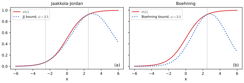
fig_S15_1. Reproduces Murphy (2023), Supplement Figure 15.1. Download: PDF · SVG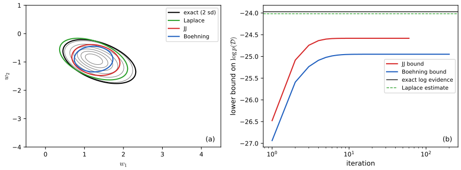
fig_15_X3. Download: PDF · SVGSee also: ml 10.6 variational logistic regression; 10.3.4 bound optimisation.
15.3.9 Case study: is Berkeley admissions biased against women?
pp. 619–621 The data (Bickel et al. 1975) have 12 rows, the applicants and admissions of men and women to six departments (4526 applications), Table 15.1. The simplest model is binomial logistic regression \(A_i\sim\Bin(N_i,\mu_i)\), \(\logit\mu_i=\alpha+\beta\,\mathrm{MALE}[i]\) with \(\alpha\sim\N(0,10)\), \(\beta\sim\N(0,1.5)\) (15.153)–(15.156), or symmetrically \(\logit\mu_i=\alpha_{\mathrm{GENDER}[i]}\), \(\alpha_j\sim\N(0,1.5)\) (15.157)–(15.159), which treats the genders equally a priori. HMC gives the 89% intervals below. The model fits badly (Figure 15.9a) and says men have a 14% higher chance of admission, even though women's rate is higher in four of the six departments. Women applied more to the harder departments. Adding department effects, \(\logit\mu_i=\alpha_{\mathrm{GENDER}[i]}+\gamma_{\mathrm{DEPT}[i]}\), \(\gamma_k\sim\N(0,1.5)\) (15.160)–(15.163), fits well (Figure 15.9b) and the gap becomes \([-0.05,0.01]\). The DAG of Figure 15.10a (\(G\to D\to A\), \(G\to A\)) justifies conditioning on \(D\); with an unobserved confounder \(U\) of \(D\) and \(A\) (Figure 15.10b) conditioning on the collider \(D\) opens the path \(G\to D\leftarrow U\to A\) and the causal conclusion fails (All of Statistics Chapter 16).
| Dept | A | B | C | D | E | F |
|---|---|---|---|---|---|---|
| men | 512 / 825 | 353 / 560 | 120 / 325 | 138 / 417 | 53 / 191 | 22 / 373 |
| women | 89 / 108 | 17 / 25 | 202 / 593 | 131 / 375 | 94 / 393 | 24 / 341 |
Filling the gap 15.21: Berkeley, Simpson's paradox and what each posterior is estimating pp. 619–621
Derivation
The gender-only model is the pooled counts. The log likelihood is \(\sum_i[A_i\eta_{g(i)}-N_i\log(1+e^{\eta_{g(i)}})]\), which depends on the data only through the pooled counts per gender. So \(\sigma(\alpha_g)\) is estimated by the pooled admission rate: 1198 of 2691 applicants for men (44.5%) and 557 of 1835 for women (30.4%). The posterior of \(\sigma(\alpha_1)-\sigma(\alpha_2)\) has mean 0.141 and 89% interval \([0.12,0.16]\), consistent with \(0.445-0.304\). The posterior of \(\alpha_1\) (men) is \([-0.28,-0.16]\) and of \(\alpha_2\) (women) is \([-0.91,-0.75]\) (the book prints these intervals without the minus signs; its stated gap \([0.12,0.16]\) is consistent only with the negative values). A two-dimensional grid integral reproduces the HMC means to 0.001.
Simpson's paradox. Write the pooled rate of gender \(g\) as \(\sum_dw_{d\mid g}r_{dg}\): the share \(w_{d\mid g}\) of that gender's applications going to department \(d\), times the departmental rate \(r_{dg}\). Take the subtable of departments A and F. Women: \(89/108=0.82\) in A and \(24/341=0.07\) in F; men: \(512/825=0.62\) and \(22/373=0.06\). Women are ahead in both departments, yet pooled they have \((89+24)/(108+341)=0.25\) against \((512+22)/(825+373)=0.45\) for men, because 76% of the women's applications in this subtable go to department F (rate 6 to 7%) while 69% of the men's go to department A. The reversal needs only that the weights differ, \(w_{d|\rm women}\ne w_{d|\rm men}\), in a way correlated with the rates. In the full table women have the higher rate in four of the six departments (A, B, D, F) and the lower pooled rate.
The department model. It conditions on \(D\), so the contrast \(\sigma(\alpha_1)-\sigma(\alpha_2)\) is a within-department contrast (an average over the departments' baseline rates); its posterior is centred at \(-0.02\), with an interval containing 0. But the posterior only says what the data and the DAG with no hidden confounders imply; with the confounder \(U\) of Figure 15.10b the contrast estimates a collider-biased quantity, so no causal sentence follows from a regression coefficient alone. This is the caution of All of Statistics, Chapter 16 and Chapter 36 of the book.
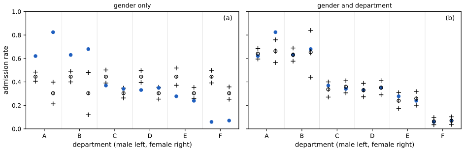
fig_15_9, own HMC with 4000 draws. Reproduces Murphy (2023), Figure 15.9. Download: PDF · SVGS15.2 Converting multinomial logistic regression to Poisson regression; beta-binomial and Poisson regression (supplement)
Supplement pp. 167–168 Multinomial as Poisson. A multinomial logistic model with \(K\) outputs can be written as \(K\) separate Poisson regressions whose counts are implicitly coupled through the total; this helps training when \(K\) is large (Taddy 2015). For \(K=2\) with \(m\) trials, \(p(y_1,y_2\given m,\mu_1,\mu_2)=\frac{m!}{y_1!y_2!}\mu_1^{y_1}\mu_2^{y_2}\) (S15.52); with \(\Lambda=\lambda_1+\lambda_2\) and \(\mu_k=\lambda_k/\Lambda\) it equals \(p(y_1)p(y_2)/p(m)\) with \(y_k\sim\mathrm{Poi}(\lambda_k)\) and \(m\sim\mathrm{Poi}(\Lambda)\) (S15.56).
Filling the gap 15.22: independent Poissons, conditioned on their total, are multinomial (S15.52)–(S15.56) Supplement p. 167
Derivation
Let \(y_k\sim\mathrm{Poi}(\lambda_k)\) independently, \(k=1..K\), and \(m=\sum_ky_k\). Sums of independent Poissons are Poisson, so \(m\sim\mathrm{Poi}(\Lambda)\), \(\Lambda=\sum\lambda_k\). For counts with \(\sum y_k=m\), \[ p(y\given m)=\frac{\prod_ke^{-\lambda_k}\lambda_k^{y_k}/y_k!}{e^{-\Lambda}\Lambda^m/m!}=\frac{m!}{\prod_ky_k!}\prod_k\Big(\frac{\lambda_k}\Lambda\Big)^{y_k}, \] using \(\prod_ke^{-\lambda_k}=e^{-\Lambda}\). This is the multinomial with probabilities \(\mu_k=\lambda_k/\Lambda\). Conversely \(p(y_1,y_2\mid m,\mu)\,p(m)=\prod_k\mathrm{Poi}(y_k\given\lambda_k)\), the equation (S15.56). Regression form. If \(\log\lambda_{nk}=a_n+w_k^\T x_n\) with a free offset \(a_n\) per observation, then \(\mu_{nk}=\softmax_k(w_k^\T x_n)\) does not depend on \(a_n\); the Poisson likelihood factorises into the multinomial likelihood of the \(y_n\) given \(m_n\) times a Poisson likelihood of \(m_n\) that involves only \(a_n\), so maximising over the \(a_n\) leaves the multinomial regression, and the \(K\) Poisson regressions can be fitted separately. Berkeley. Fitting one Poisson rate each to the 12 admission counts and the 12 rejection counts gives \(\hat\lambda_1=146.2\), \(\hat\lambda_2=230.9\) (their means) and the admission rate \(\hat\lambda_1/(\hat\lambda_1+\hat\lambda_2)=0.388\), equal to the pooled binomial rate \(\sum A_i/\sum N_i=1755/4526=0.388\) (S15.72), (S15.75).
Supplement pp. 167–169 Beta-binomial regression. If the counts vary more than a binomial allows (overdispersion), use \(y_i\sim\mathrm{BetaBinom}(m_i,\alpha_i,\beta_i)\), \(\alpha_i=\pi_i\kappa\), \(\beta_i=(1-\pi_i)\kappa\), \(\pi_i=\sigma(w^\T x_i)\) (S15.57)–(S15.60): the mean \(\pi_i\) depends on the inputs, the shape \(\kappa=\alpha+\beta\) is shared, and \(\mathrm{BetaBinom}(y\given m,\alpha,\beta)=\int\Bin(y\given m,\mu)\mathrm{Beta}(\mu\given\alpha,\beta)\d\mu\) (S15.63). For the Berkeley data with gender only, the model \(A_i\sim\mathrm{BetaBinom}(N_i,\pi_i,\kappa)\), \(\logit\pi_i=\alpha_{\mathrm{GENDER}[i]}\), \(\alpha_j\sim\N(0,1.5)\), \(\kappa=\phi+2\), \(\phi\sim\mathrm{Exp}(1)\) (S15.64)–(S15.68) is no longer overconfident: its predictions are broad, the male and female admission rates have heavily overlapping posteriors and the false conclusion of bias is avoided, but the model is nearly uninformative.
Filling the gap 15.23: the beta-binomial's overdispersion (S15.57)–(S15.63) Supplement pp. 167–168
Derivation
Let \(\mu\sim\mathrm{Beta}(\pi\kappa,(1-\pi)\kappa)\) and \(y\given\mu\sim\Bin(m,\mu)\). The Beta has mean \(\pi\) and variance \(\frac{\pi(1-\pi)}{\kappa+1}\). By iterated expectations \(\E[y]=m\pi\). By the law of total variance, \(\var[y]=\E[m\mu(1-\mu)]+\var[m\mu]=m(\pi-\E\mu^2)+m^2\frac{\pi(1-\pi)}{\kappa+1}\), and \(\E\mu^2=\var\mu+\pi^2\), so \[ \var[y]=m\pi(1-\pi)\Big[1-\frac1{\kappa+1}+\frac m{\kappa+1}\Big]=m\pi(1-\pi)\,\frac{m+\kappa}{1+\kappa}. \] Compared with the binomial variance \(m\pi(1-\pi)\) the factor \(\frac{m+\kappa}{1+\kappa}\ge1\) is the overdispersion, tending to 1 as \(\kappa\to\infty\) (the Beta collapses to a point). It grows with the group size \(m\): large departments are the most dispersed. In the Berkeley fit the posterior mean of \(\kappa\) is 3.0, so a department with \(m=500\) applicants has variance about 125 times the binomial one, which is why the predictions are so wide. (The constraint \(\kappa>2\) of the text rules out \(\alpha+\beta<2\); a density can still diverge at an endpoint if \(\pi\kappa<1\).) The pmf agrees with the library implementation.
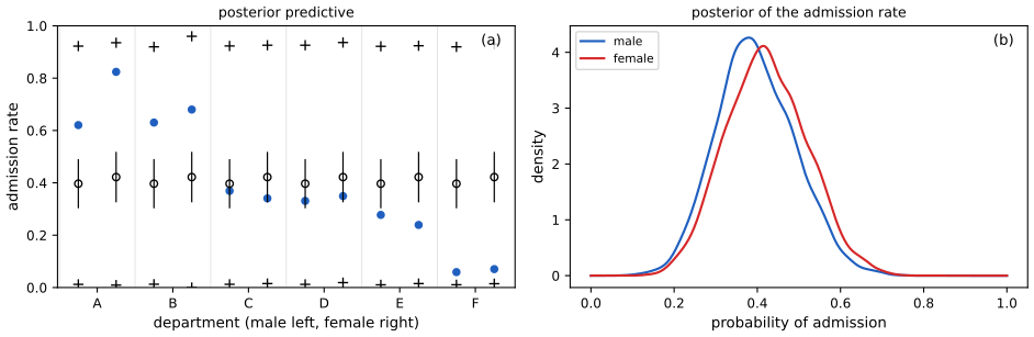
fig_S15_2. Reproduces Murphy (2023), Supplement Figure 15.2. Download: PDF · SVGSupplement pp. 168–169 Poisson regression for the same data models the two columns of counts as \(y_{j,n}\sim\mathrm{Poi}(\lambda_j)\), \(\lambda_j=e^{\alpha_j}\), \(\alpha_j\sim\N(0,1.5)\) (S15.69)–(S15.71) (\(j=1\) admitted, \(j=2\) rejected, \(n=1..12\)). The implied admission rate \(\hat\lambda_1/(\hat\lambda_1+\hat\lambda_2)=0.38\) equals the binomial model's \(\sigma(\hat\alpha)=0.38\) with \(A_n\sim\Bin(m_n,\sigma(\alpha))\) (S15.72)–(S15.75), as gap 15.22 explains.
15.4 Probit regression
p. 621 Probit regression uses \(\mu_n=\Phi(a_n)\), \(a_n=w^\T x_n\), instead of \(\sigma(a_n)\); the link \(\Phi^{-1}\) is the probit function. \(\Phi\) is very close to a rescaled sigmoid (Figure 15.11, above), so predictions are similar, but probit has a simple latent-variable interpretation (from choice theory in economics) that makes Bayesian inference easier.
15.4.1 Latent variable interpretation
pp. 621–622 Let \(z_n=w^\T x_n+\epsilon_n\) with \(\epsilon_n\sim\N(0,1)\) be a latent preference and \(y_n=\ind(z_n\ge0)\) (15.164). Marginalising \(z_n\), \(p(y_n=1)=\Pr(\epsilon_n\ge-w^\T x_n)=1-\Phi(-w^\T x_n)=\Phi(w^\T x_n)\) (15.165)–(15.167). Logistic regression is the same with logistic noise \(f(y\given\mu,s)=\frac{e^{-(y-\mu)/s}}{s(1+e^{-(y-\mu)/s})^2}\) (15.168) of variance \(s^2\pi^2/3\) and cdf (15.169), but Gaussian noise is computationally easier.
Filling the gap 15.24: the logistic noise model and the probit gradient and Hessian (15.164)–(15.171) pp. 621–622
Derivation
Logistic noise. With \(\epsilon\) logistic(0,1), \(F(t)=\Pr(\epsilon\le t)=1/(1+e^{-t})\), and \(\Pr(\epsilon\ge-\eta)=1-F(-\eta)=1-\frac1{1+e^{\eta}}=\frac1{1+e^{-\eta}}=\sigma(\eta)\). Its density \(F'=F(1-F)=\frac{e^{-t}}{(1+e^{-t})^2}\) matches (15.168) at \(\mu=0,s=1\) (the book's form \(\frac1{4s}\operatorname{sech}^2\frac{y-\mu}{2s}\) is the same function), and the variance is \(\pi^2/3\). A Gaussian noise of variance 1 corresponds to a logistic noise of scale \(s\) with \(s^2\pi^2/3=1\) by variance matching, \(s=\sqrt3/\pi\), so the logistic coefficients are about \(\pi/\sqrt3=1.8\) times the probit ones (matching slopes at 0 instead gives \(1/\lambda=\sqrt{8/\pi}=1.6\): the usual rule of thumb is 1.6 to 1.8).
Gradient and Hessian. Let \(\tilde y_n=2y_n-1\in\{\pm1\}\), so \(p(y_n\given\eta_n)=\Phi(\tilde y_n\eta_n)\) (by symmetry \(\Phi(-\eta)=1-\Phi(\eta)\)). Then \(\frac{\d}{\d\eta}\log\Phi(\tilde y\eta)=\tilde y\frac{\phi(\tilde y\eta)}{\Phi(\tilde y\eta)}=\tilde y\frac{\phi(\eta)}{\Phi(\tilde y\eta)}\) (\(\phi\) is even), which with \(\partial\eta/\partial w=x_n\) is (15.170). Differentiating once more, with \(\phi'(\eta)=-\eta\phi(\eta)\) and \(\tilde y^2=1\): \[ \frac{\d^2}{\d\eta^2}\log\Phi(\tilde y\eta)=\tilde y\,\frac{-\eta\phi\,\Phi(\tilde y\eta)-\phi\cdot\tilde y\phi}{\Phi(\tilde y\eta)^2}=-\Big[\frac{\phi(\eta)^2}{\Phi(\tilde y\eta)^2}+\frac{\tilde y\eta\,\phi(\eta)}{\Phi(\tilde y\eta)}\Big], \] which gives (15.171) (the book's \(H_n\) is the Hessian of the log likelihood, hence the minus sign; the NLL Hessian is \(+X^\T\diag(\cdot)X\)). The bracket is positive (\(\log\Phi\) is strictly concave), so the penalised probit NLL is strictly convex and any quasi-Newton method converges to the unique optimum. Both formulas match finite differences.
15.4.2 Maximum likelihood estimation
pp. 622–624 SGD. With the gradient (15.170) and Hessian (15.171), any gradient-based optimiser works. EM. With the latent \(z\) the complete-data log likelihood under a \(\N(0,V_0)\) prior is \(\ell(z,w)=\sum_n\log p(y_n\given z_n)-\frac12(z-Xw)^\T(z-Xw)-\frac12w^\T V_0^{-1}w\) (15.172), (15.173). The E step needs the posterior of \(z_n\), a truncated normal (15.174), with mean \[ \E[z_n\given y_n,x_n,w]=\begin{cases}\mu_n+\dfrac{\phi(\mu_n)}{\Phi(\mu_n)}&y_n=1\\[2mm]\mu_n-\dfrac{\phi(\mu_n)}{\Phi(-\mu_n)}&y_n=0\end{cases}\quad(15.175),\ \ \mu_n=w^\T x_n, \] and the M step is ridge regression of \(\E[z]\) on \(X\): \(\hat w=(V_0^{-1}+X^\T X)^{-1}X^\T\E[z]\) (15.176). EM is simple but can be much slower than a gradient method, because the E-step posterior has high entropy (only the sign of \(z\) is known); a stronger regulariser helps.
Filling the gap 15.25: the probit EM steps, why EM is slow, and the Albert-Chib sampler (15.172)–(15.180) pp. 622–624
Derivation
E step. Given \(y_n=1\), the posterior of \(z_n\) is \(\N(\mu_n,1)\) restricted to \(z>0\) (the likelihood \(p(y_n=1\given z_n)=\ind(z_n>0)\)). For \(z\sim\N(\mu,1)\) and \(a=-\mu\): \(\E[z\given z>0]=\mu+\E[\varepsilon\given\varepsilon>-\mu]=\mu+\frac{\phi(-\mu)}{1-\Phi(-\mu)}=\mu+\frac{\phi(\mu)}{\Phi(\mu)}\) (the mean of a one-sided truncated standard normal is \(\phi(a)/(1-\Phi(a))\): integrate \(\varepsilon\phi(\varepsilon)=-\phi'(\varepsilon)\)). Given \(y_n=0\): \(\E[z\given z<0]=\mu-\frac{\phi(-\mu)}{\Phi(-\mu)}=\mu-\frac{\phi(\mu)}{\Phi(-\mu)}\): (15.175). Both agree with the library truncated-normal mean.
M step. \(Q(w)=\E[\ell(z,w)]\) depends on \(z\) only through the linear and the quadratic term \(-\frac12\E\|z-Xw\|^2=-\frac12\|\E z-Xw\|^2+\mathrm{const}\), so the maximiser is the ridge solution (15.176).
Why EM is slow. The EM rate of convergence near the optimum is the largest eigenvalue of \(I_{\rm mis}I_{\rm com}^{-1}\) (the fraction of missing information); here the complete information is \(X^\T X+V_0^{-1}\) while the observed information is smaller, because we only see the sign of \(z\). With a stronger prior \(V_0^{-1}\), the complete information grows relative to the missing part and the rate improves. In Figure 15.12, BFGS converges in 13 iterations and EM needs 92 iterations to reach \(10^{-8}\) of the optimal value.
Gibbs sampler (Albert and Chib 1993). Given \(w\), the \(z_n\) are independent truncated normals (15.177), sampled by inverse-cdf: for \(z_n>0\), draw \(u\sim U(\Phi(-\mu_n),1)\) and set \(z_n=\mu_n+\Phi^{-1}(u)\); for \(z_n<0\), \(u\sim U(0,\Phi(-\mu_n))\) (the quantile of \(\N(\mu,\sigma^2)\) truncated to \([a,b]\) is \(\mu+\sigma\Phi^{-1}(u)\) with \(u\sim U(\Phi(\frac{a-\mu}\sigma),\Phi(\frac{b-\mu}\sigma))\)). Given \(z\) the model is conjugate linear-Gaussian, so \(w\given z\sim\N(w_N,V_N)\) with \(V_N=(V_0^{-1}+X^\T X)^{-1}\), \(w_N=V_N(V_0^{-1}w_0+X^\T z)\) (15.178)–(15.180) by Bayes' rule for Gaussians. The sampler's posterior mean agrees with a grid integration of the posterior on a two-weight example.
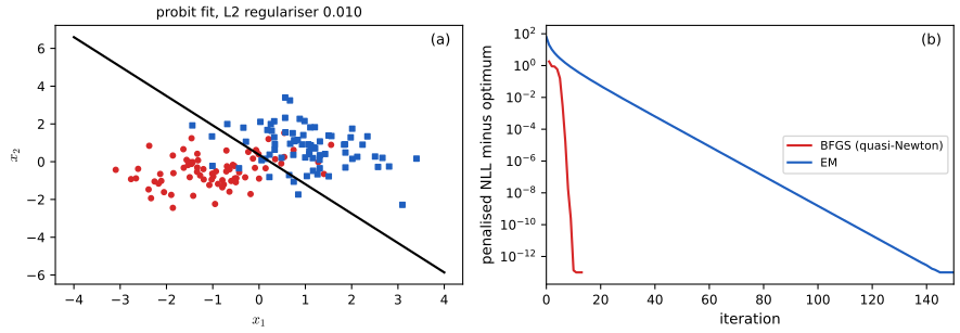
fig_15_12. Reproduces Murphy (2023), Figure 15.12. Download: PDF · SVG15.4.3 Bayesian inference
p. 624 The latent-variable form gives a Gibbs sampler (Albert and Chib 1993): alternate \(z_i\given y_i,x_i,w\) (a truncated Gaussian, (15.177), sampled by inverse cdf) and \(w\given z\) (a Gaussian, (15.178)–(15.180)); see gap 15.25. Variational Bayes is typically much faster.
15.4.4 Ordinal probit regression
p. 624 If the response is ordered (low, medium, high), introduce \(C+1\) thresholds \(\gamma_0\le\dots\le\gamma_C\) and set \(y_n=j\) iff \(\gamma_{j-1}<z_n\le\gamma_j\) (15.181), with \(\gamma_0=-\infty\), \(\gamma_1=0\), \(\gamma_C=\infty\) for identifiability. For \(C=2\) this is binary probit. Fitting needs a constrained optimisation over \(w\) and \(\gamma\) (an EM version exists, Kawakatsu and Largey 2009) or a Gibbs sampler (Hoff 2009).
Filling the gap 15.26: category probabilities and identifiability of ordinal probit (15.181) p. 624
Derivation
With \(z=w^\T x+\epsilon\), \(\epsilon\sim\N(0,1)\), \(\Pr(y=j)=\Pr(\gamma_{j-1}<z\le\gamma_j)=\Phi(\gamma_j-w^\T x)-\Phi(\gamma_{j-1}-w^\T x)\), and cumulatively \(\Pr(y\le j)=\Phi(\gamma_j-w^\T x)\) (the probit analogue of the proportional-odds logistic model). Identifiability: adding a constant \(c\) to every threshold and to an intercept in \(w^\T x\) leaves all probabilities unchanged, so one threshold is fixed (\(\gamma_1=0\)); the noise variance is fixed at 1 because multiplying \(z\), \(w\) and \(\gamma\) by \(k>0\) also leaves them unchanged. With \(C=3\) classes there is one free threshold \(\gamma_2>0\) which sets the relative masses of the three intervals: with \(w^\T x=0\), \(\Pr(y=1)=\frac12\), \(\Pr(y=2)=\Phi(\gamma_2)-\frac12\), \(\Pr(y=3)=1-\Phi(\gamma_2)\). The constraint \(\gamma_{j-1}\le\gamma_j\) is why direct optimisation needs care (reparametrise by positive increments).
15.4.5 Multinomial probit models
pp. 624–625 For unordered \(y_n\in\{1,\dots,C\}\), let \(z_{nc}=w_c^\T x_{nc}+\epsilon_{nc}\), \(\epsilon\sim\N(0,R)\) (15.182), (15.183) and \(y_n=\argmax_cz_{nc}\) (15.184). Unlike multinomial logistic regression, the errors may be correlated through \(R\), removing the independence of irrelevant alternatives property; only utility differences matter, so \(R\) must be constrained for identifiability. Replacing the argmax by \(y_{nc}=\ind(z_{nc}>0)\) gives the multivariate probit for \(C\) correlated binary outcomes (Tang et al. 2012). See Greene and others (references in the book) for details.
15.5 Multilevel (hierarchical) GLMs
pp. 625–626 Suppose we have \(J\) related datasets \(\mathcal D_j=\{(x_n^j,y_n^j)\}_{n=1}^{N_j}\). Fitting \(J\) separate models overfits small groups, pooling everything underfits, and a hierarchical (multilevel, partially pooled) model gives each group its own parameter \(\theta_j\) drawn from a shared distribution \(p(\theta_0)\): \[ p(\theta_{0:J},\mathcal D)=p(\theta_0)\prod_{j=1}^J\Big[p(\theta_j\given\theta_0)\prod_{n=1}^{N_j}p(y_n^j\given x_n^j,\theta_j)\Big]\tag{15.185} \] (Figure 15.13a). Equivalently, with a group indicator \(g_n\in\{1,\dots,J\}\), \(p(\theta_{0:J},\mathcal D)=p(\theta_0)\prod_jp(\theta_j\given\theta_0)\prod_np(y_n\given x_n,\theta_{g_n})\) (15.186), (15.187) (Figure 15.13b). With a GLM likelihood this is a hierarchical GLM (Lee and Nelder 1996); see Gelman and Hill (2007).
15.5.1 Generalized linear mixed models (GLMMs)
p. 626 With a Gaussian group prior \(p(\theta_j\given\theta_0)=\N(\theta_0,\Sigma)\): \(\eta_n=x_n^\T\theta_{g_n}=x_n^\T\theta_0+x_n^\T\epsilon_{g_n}\), \(\epsilon_j\sim\N(0,\Sigma)\) (15.188), (15.189): \(\theta_0\) are the fixed effects, the \(\epsilon_j\) the random effects (group-specific deviations, correlated within a group), a GLMM. Any inference method of Section 15.1.4 applies.
Filling the gap 15.27: partial pooling as a precision-weighted average, and the latent intraclass correlation pp. 625–626
Derivation
Normal-normal pooling. For a group with \(n\) Gaussian observations \(y_i\sim\N(\alpha,\sigma^2)\) and \(\alpha\sim\N(\mu,\tau^2)\), the posterior of \(\alpha\) is Gaussian with precision \(\frac n{\sigma^2}+\frac1{\tau^2}\) and mean \[ \frac{n\bar y/\sigma^2+\mu/\tau^2}{n/\sigma^2+1/\tau^2}=(1-B)\,\bar y+B\,\mu,\qquad B=\frac{\sigma^2}{\sigma^2+n\tau^2}\in(0,1), \] (Gaussian conjugacy; ml 3.3.1). The shrinkage weight \(B\) is large when the group is small (\(n\) small), noisy (\(\sigma^2\) large) or the groups are similar (\(\tau^2\) small). The limits are the two extremes of the introduction: \(\tau\to\infty\) gives \(B\to0\) (no pooling: each group uses its own mean), \(\tau\to0\) gives \(B\to1\) (complete pooling). In a regression the same formula holds for each group's intercept given the other parameters, with \(\bar y\) the mean of the partial residuals \(y_i-\beta_jx_i\). In the radon example the exact conditional posterior of a county intercept given the other parameters is this precision-weighted average (confirmed by minimising the conditional log density at a posterior draw). The full posterior also averages over the uncertainty in \((\mu,\tau,\sigma)\), which is why the hierarchical fit is the right compromise (Figure 15.16): its county lines are closer to the simulated truth (root mean square error 0.22 against 0.41 for separate fits).
Random effects induce correlation. For two observations \(n,m\) in the same group with random effect \(\epsilon\sim\N(0,\Sigma)\), \(\cov(\eta_n,\eta_m)=x_n^\T\Sigma x_m\); observations in different groups are independent given \(\theta_0\). For a random intercept \(b_j\sim\N(0,\sigma_b^2)\) in logistic regression, the latent-variable form \(y^*=\eta+b_j+\epsilon\), with logistic \(\epsilon\) (gap 15.24), gives within-group latent correlation (the intraclass correlation) \[ \rho=\frac{\sigma_b^2}{\sigma_b^2+\pi^2/3},\] since \(\var[\epsilon]=\pi^2/3\). A simulation with \(\sigma_b=0.5,1,2\) matches this within 0.01. A hierarchical model therefore captures dependence that a GLM with independent rows ignores.
15.5.2 Example: radon regression
pp. 626–629 Radon, the leading cause of lung cancer in non-smokers, is regressed (log level) on a county indicator and whether the measurement was on the basement (\(x=0\)) or first floor (\(x=1\)): \(p(y_n\given x_n,g_n=j,\theta)=\N(\alpha_j+\beta_jx_n,\sigma_y^2)\) (15.190), with \(\alpha_j\sim\N(\mu_\alpha,\sigma_\alpha^2)\), \(\beta_j\sim\N(\mu_\beta,\sigma_\beta^2)\), and weak priors \(\mu_\alpha,\mu_\beta\sim\N(0,1)\), \(\sigma_\alpha,\sigma_\beta,\sigma_y\sim\mathcal C^+(1)\) (Figure 15.14). The book uses 85 Minnesota counties with 2 to 80 measurements each. Posterior inference. \(\mu_\beta\) is near \(-0.6\) (first floors have less radon), the \(\alpha_j\) vary a lot (Figure 15.15), and the hierarchical fit predicts sensibly even in counties lacking some covariate combination (Figure 15.16); its posterior-predictive RMSE is 0.08 against 0.13 for the non-hierarchical model.
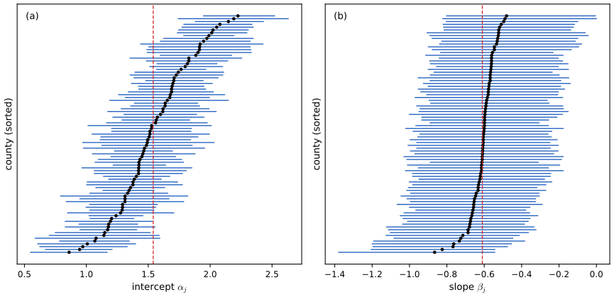
fig_15_15. Reproduces Murphy (2023), Figure 15.15. Download: PDF · SVG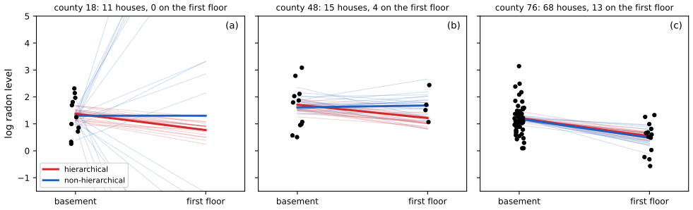
fig_15_16. Reproduces Murphy (2023), Figure 15.16. Download: PDF · SVGNon-centred parameterisation. Hierarchical posteriors often have strongly correlated parameters: Figure 15.17a shows \(p(\beta_j,\sigma_\beta\given\mathcal D)\) for one county, a funnel (Neal 2003): large \(\sigma_\beta\) lets \(\beta_j\) vary widely, small \(\sigma_\beta\) pins \(\beta_j\) to \(\mu_\beta\). Samplers struggle at the neck, and the histogram of \(\sigma_\beta\) excludes \([0,0.1]\), ruling out shrinking \(\beta_j\) all the way to 0, which matters for sparsity. Write \(\beta_j=\mu_\beta+\tilde\beta_j\sigma_\beta\) with \(\tilde\beta_j\sim\N(0,1)\) (Papaspiliopoulos et al. 2003), which removes most of the correlation (Figure 15.17b); see 12.6.5.
Filling the gap 15.28: why the centred hierarchy has a funnel and how the non-centred form removes it pp. 628–629
Derivation
The funnel. In the centred form the prior density of a group effect is \(p(\beta_j\given\mu,\sigma)=\sigma^{-1}\phi((\beta_j-\mu)/\sigma)\): for fixed \(\sigma\) a Gaussian of width \(\sigma\), and its height scales as \(1/\sigma\). So the joint \((\beta_j,\log\sigma)\) of the prior (with, say, a flat \(\log\sigma\)) is a funnel: wide where \(\log\sigma\) is large, a narrow neck of width \(\sigma\) where it is small. When group \(j\) has few data, the likelihood \(\prod_np(y_n\given\beta_j)\) is flat over the neck and the posterior inherits the funnel. A fixed-step-size Hamiltonian or random-walk sampler cannot suit both regions: a step small enough for the neck explores the mouth slowly, a step large enough for the mouth diverges in the neck (divergent transitions) and leaves the neck unvisited, biasing \(\sigma\) upwards (Figure 15.17a).
The transformation. Define \(\tilde\beta_j=(\beta_j-\mu)/\sigma\), a bijection of \(\beta_j\) for each \(\sigma>0\). Under the prior \(\tilde\beta_j\sim\N(0,1)\) independently of \((\mu,\sigma)\): the transformed prior is a product of independent factors with no funnel, and the original \(\beta_j=\mu+\sigma\tilde\beta_j\) has exactly the law \(\N(\mu,\sigma^2)\) (the Gaussian location-scale property). Posterior dependence between \(\tilde\beta_j\) and \(\sigma\) now enters only through the likelihood \(\prod_np(y_n\given\mu+\sigma\tilde\beta_j)\), which for a data-poor group is flat in \(\tilde\beta_j\) and so adds no correlation. The reverse holds for a data-rich group: there the likelihood pins \(\beta_j\) and the centred form is better (Papaspiliopoulos et al. 2003). Numbers. For the same county as Figure 15.17 (4 houses) the effective sample size of \(\sigma_\beta\) is 34 per 1000 draws in the centred run against 229 in the non-centred run, and the smallest \(\sigma_\beta\) ever visited is 0.064 against 0.001. (With this simulated data no divergence is flagged, because the true \(\sigma_\beta=0.2\) is not small; the symptom is poor mixing, not failure.)
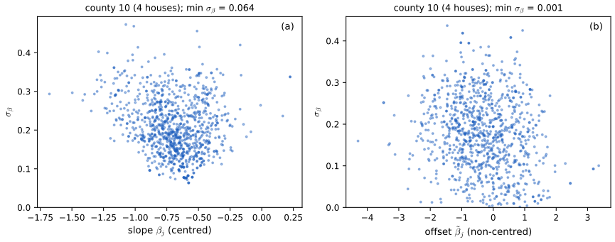
fig_15_17 (two HMC runs of the whole model). Reproduces Murphy (2023), Figure 15.17. Download: PDF · SVGSee also: hierarchical shrinkage demo (Chapter 3), 12.6.5 Neal's funnel.
S15.3 GLMM (hierarchical Bayes) regression (supplement)
Supplement pp. 169–171 Back to the Berkeley data, grouped by department and gender: a varying intercept and slope model uses \(A_i\sim\Bin(N_i,\mu_i)\), \(\logit\mu_i=\alpha_{\mathrm{DEPT}[i]}+\beta_{\mathrm{DEPT}[i]}\,\mathrm{MALE}[i]\) (S15.76), (S15.77), with correlated pairs \((\alpha_j,\beta_j)\sim\N((\alpha,\beta)^\T,\Sigma)\), \(\alpha\sim\N(0,4)\), \(\beta\sim\N(0,1)\), \(\Sigma=\diag(\sigma)R\diag(\sigma)\), \(R\sim\mathrm{LKJ}(2)\), \(\sigma_d\sim\N^+(0,1)\) (S15.78)–(S15.83); here the second argument of \(\N\) is a standard deviation. Compactly, \(w_j=(\alpha_j,\beta_j)\sim\N(u,\Sigma)\), \(u\sim\N(0,\diag(4,1))\). In the non-centred form (Section 15.5.2), \(w_j=u+\diag(\sigma)Lz_j\) with \(L=\mathrm{chol}(R)\), \(z_j\sim\N(0,I_2)\), \(v_j=\diag(\sigma)Lz_j\) and \(\logit\mu_i=u_0+v_{\mathrm{DEPT}[i],0}+(u_1+v_{\mathrm{DEPT}[i],1})\mathrm{MALE}[i]\) (S15.87)–(S15.91). (The draft writes \(\log(\mu_i)\) in (S15.84) and (S15.91), which must be \(\logit(\mu_i)\).) The fit is slightly better than the model of Figure 15.9b, especially for women in department 2 (Figure S15.3).
Filling the gap 15.29: the non-centred Cholesky form and the LKJ prior in two dimensions (S15.78)–(S15.91) Supplement pp. 169–171
Derivation
Covariance. If \(z_j\sim\N(0,I_2)\) and \(R=LL^\T\), then \(v_j=\diag(\sigma)Lz_j\) has covariance \(\diag(\sigma)LL^\T\diag(\sigma)=\diag(\sigma)R\diag(\sigma)=\Sigma\), and it is Gaussian: so \(w_j=u+v_j\sim\N(u,\Sigma)\) exactly (S15.87), and the prior of \(z_j\) is free of \((u,\sigma,R)\), as in the non-centred argument of gap 15.28. For \(2\times2\), \(R=\begin{pmatrix}1&r\\r&1\end{pmatrix}\) and \(L=\begin{pmatrix}1&0\\r&\sqrt{1-r^2}\end{pmatrix}\): \(v_{j,0}=\sigma_0z_{j,0}\), \(v_{j,1}=\sigma_1(rz_{j,0}+\sqrt{1-r^2}z_{j,1})\), with correlation \(r\) between the intercept and slope effects.
LKJ(2). The LKJ(\(\eta\)) density on correlation matrices is \(\propto|R|^{\eta-1}\); for \(2\times2\), \(|R|=1-r^2\), so \(p(r)\propto(1-r^2)^{\eta-1}\), and for \(\eta=2\), \(p(r)\propto1-r^2\) on \((-1,1)\) (normalising constant \(\int_{-1}^1(1-r^2)\d r=4/3\)): a gentle preference for zero correlation. An unconstrained parametrisation is \(r=\tanh\zeta\); then \(\d r=\operatorname{sech}^2\zeta\,\d\zeta=(1-r^2)\d\zeta\), so \(p(\zeta)\propto(1-r^2)^2=\operatorname{sech}^4\zeta\), with \(\int\operatorname{sech}^4\zeta\,\d\zeta=4/3\) as well (checked). This is the extra term \(2\log(1-r^2)\) in the log posterior used by the sampler, together with \(\sum_d\log\sigma_d\) for \(\sigma_d=e^{s_d}\) and the half-normal prior \(-\frac12\sigma_d^2\).
Reading the fit. The posterior mean intercept and slope sds are \(\sigma_0\approx1.4\) and \(\sigma_1\approx0.47\) on the logit scale, and the correlation \(\rho\) between the department intercept and slope has posterior mean \(-0.35\): departments with a higher base admission rate (intercept) have a more negative male slope, but with considerable uncertainty. The varying-slope model has the same number of parameters as the additive model of Section 15.3.9 but they are partly pooled.
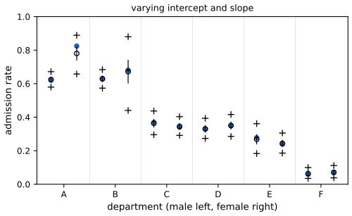
fig_S15_3. Reproduces Murphy (2023), Supplement Figure 15.3b (the graphical model in 15.3a is a diagram). Download: PDF · SVGPractice problems
The book has no exercises for this chapter. These three short problems are my own.
Practice problem 15.1 (how vague is a vague logit prior?). For \(\alpha\sim\N(0,\omega)\), what is \(\Pr(\sigma(\alpha)<0.05\text{ or }>0.95)\) for \(\omega=1.5\) and \(\omega=10\)? For which \(\omega\) is the density of \(\sigma(\alpha)\) U-shaped?
Solution
\(\sigma(\alpha)>0.95\iff\alpha>\log19=2.944\), and by symmetry the probability is \(2\Phi(-2.944/\sqrt\omega)\). For \(\omega=1.5\) (\(\sqrt\omega=1.225\)): \(2\Phi(-2.40)=0.016\). For \(\omega=10\) (\(\sqrt\omega=3.162\)): \(2\Phi(-0.931)=0.352\). The density is U-shaped (\(s=\frac12\) a local minimum) exactly when \(\omega>2\) (gap 15.16), so \(\omega=10\) is U-shaped and \(\omega=1.5\) is not.
Practice problem 15.2 (a reversal). In a two-department study, department 1 admits 90 of 100 women and 800 of 1000 men, and department 2 admits 100 of 1000 women and 5 of 100 men. Compute the rates by department and pooled, and say what drives the reversal.
Solution
Department 1: women \(0.90\), men \(0.80\). Department 2: women \(0.10\), men \(0.05\). Pooled: women \((90+100)/(100+1000)=190/1100=0.173\); men \((800+5)/(1000+100)=805/1100=0.732\). Women have the higher rate in both departments and a far lower pooled rate, because 91% of the women applied to the low-rate department 2 while 91% of the men applied to department 1: the pooled rate is a weighted average with different weights, \(\sum_dw_{d|g}r_{dg}\) (gap 15.21).
Practice problem 15.3 (to prune or not to prune). In ARD, a feature has sparsity factor \(s=4\) and quality factor \(q\). Find the optimal \(\alpha\) for \(q^2=9\) and for \(q^2=3\).
Solution
By gap 15.12 the feature is retained iff \(q^2>s\), with \(\alpha=s^2/(q^2-s)\). For \(q^2=9>4\): \(\alpha=16/5=3.2\) (the feature has prior variance \(1/\alpha\approx0.31\)). For \(q^2=3\le4\): \(L'(\alpha)\propto s^2+(s-q^2)\alpha=16+\alpha>0\) for all \(\alpha\), so \(\alpha=\infty\) and the feature is pruned.
Notes on the book
Corrections and clarifications found while checking the results numerically
- Section 15.3.9, the intervals for \(\alpha_1,\alpha_2\). The text gives the 89% intervals of the gender-only model as \([-0.29,0.16]\) for \(\alpha_1\) and \([-0.91,0.75]\) for \(\alpha_2\). HMC and a grid integral both give \([-0.28,-0.16]\) and \([-0.91,-0.75]\); the printed ones lost their minus signs (the stated difference \([0.12,0.16]\), mean 0.14, is consistent only with the negative values).
- Section 15.2.3.3, the g-prior. The text says the NIG prior has \(\breve a=-D/2\), \(\breve b=0\), but (15.81) states \(\hat a=N/2\), which requires \(\breve a=0\) (with \(\breve a=-D/2\), \(\hat a=(N-D)/2\)). Also \(s^2\) in (15.82) must be read as the residual sum of squares \(\|y-\hat y\|^2\), whereas (15.72) defines \(s^2\) with a division by \(\nu\) (gap 15.6).
- Section 15.2.5, (15.87). \(\pi\) is the probability of the slab in (15.86) but the spike in (15.87); with \(\pi=\Pr(w_d\ne0)\) the penalty weight is \(\lambda=\log\frac{1-\pi}{\pi}\) (gap 15.8).
- Section 15.1.3. "Assuming \(f(\eta_n)>0\)" should read \(f'(\eta_n)>0\) together with full column rank of \(X\); even then the MLE exists only if the data are not separable (gaps 15.3, 15.17).
- Supplement (S15.1), (S15.3), (S15.6). The likelihood of one binary observation is \(\sigma(\eta)^y(1-\sigma(\eta))^{1-y}\) (the draft prints the exponent \(1-\eta_n\)) \(=e^{\eta y}\sigma(-\eta)\); the draft prints \(e^{-\eta y}\sigma(-\eta)\) in (S15.3) and (S15.6). The correct sign is the one that gives the linear term \(\eta_n(y_n-\frac12)\) in (S15.8).
- Supplement (S15.84), (S15.91). The linear predictor is on the logit scale: \(\logit(\mu_i)=\dots\), not \(\log(\mu_i)\) (compare (S15.77)).
- (15.102). \(\ell(\alpha,\beta)=\log|C_\alpha|+y^\T C_\alpha^{-1}y\) equals \(-2\log p(y\given X,\alpha,\beta)\) only up to the constant \(N\log2\pi\).
References
- Murphy, K. P. (2023). Probabilistic Machine Learning: Advanced Topics. MIT Press, Cambridge, MA. Chapter 15, pp. 591–630, and online supplement, Chapter 15. probml.github.io/pml-book/book2.html.
- Albert, J. H. and Chib, S. (1993). Bayesian analysis of binary and polychotomous response data. Journal of the American Statistical Association, 88(422), 669–679.
- Bickel, P. J., Hammel, E. A. and O'Connell, J. W. (1975). Sex bias in graduate admissions: data from Berkeley. Science, 187(4175), 398–404.
- Böhning, D. (1992). Multinomial logistic regression algorithm. Annals of the Institute of Statistical Mathematics, 44(1), 197–200.
- Carvalho, C. M., Polson, N. G. and Scott, J. G. (2010). The horseshoe estimator for sparse signals. Biometrika, 97(2), 465–480.
- Gelman, A. and Hill, J. (2007). Data Analysis Using Regression and Multilevel/Hierarchical Models. Cambridge University Press.
- Gelman, A., Jakulin, A., Pittau, M. G. and Su, Y.-S. (2008). A weakly informative default prior distribution for logistic and other regression models. Annals of Applied Statistics, 2(4), 1360–1383.
- Jaakkola, T. S. and Jordan, M. I. (2000). Bayesian parameter estimation via variational methods. Statistics and Computing, 10(1), 25–37.
- MacKay, D. J. C. (1992). Bayesian interpolation. Neural Computation, 4(3), 415–447.
- Makalic, E. and Schmidt, D. F. (2016). A simple sampler for the horseshoe estimator. IEEE Signal Processing Letters, 23(1), 179–182.
- Menon, A. K., Jayasumana, S., Rawat, A. S., Jain, H., Veit, A. and Kumar, S. (2021). Long-tail learning via logit adjustment. International Conference on Learning Representations.
- Mitchell, T. J. and Beauchamp, J. J. (1988). Bayesian variable selection in linear regression. Journal of the American Statistical Association, 83(404), 1023–1032.
- Neal, R. M. (2003). Slice sampling. Annals of Statistics, 31(3), 705–767.
- Papaspiliopoulos, O., Roberts, G. O. and Sköld, M. (2003). Non-centered parameterisations for hierarchical models and data augmentation. In Bayesian Statistics 7. Oxford University Press.
- Park, T. and Casella, G. (2008). The Bayesian lasso. Journal of the American Statistical Association, 103(482), 681–686.
- Taddy, M. (2015). Distributed multinomial regression. Annals of Applied Statistics, 9(3), 1394–1414.
- Tipping, M. E. (2001). Sparse Bayesian learning and the relevance vector machine. Journal of Machine Learning Research, 1, 211–244.
- Tipping, M. E. and Faul, A. C. (2003). Fast marginal likelihood maximisation for sparse Bayesian models. Artificial Intelligence and Statistics.
- Wipf, D. and Nagarajan, S. (2010). Iterative reweighted \(\ell_1\) and \(\ell_2\) methods for finding sparse solutions. IEEE Journal of Selected Topics in Signal Processing, 4(2), 317–329.
- Zellner, A. (1986). On assessing prior distributions and Bayesian regression analysis with g-prior distributions. In Bayesian Inference and Decision Techniques, North-Holland.