Generative models: an overview
A generative model is a distribution over data, possibly conditioned on an input. This chapter opens Part IV with a map: the six families of deep generative model (variational autoencoders, autoregressive models, flows, diffusion models, energy-based models and GANs) compared on density, sampling, training, latents and architecture; the goals a generative model serves, from sampling and density estimation to imputation, interpolation and compression; and, in most detail, the problem of evaluation, where likelihood, perplexity, the Inception score, the Fréchet distance and precision and recall each see only part of what matters. The notes prove what the book states without proof and show, on two-dimensional data, what each score can and cannot detect.
Ch. 1 Introduction Ch. 2 Probability Ch. 3 Statistics Ch. 4 Graphical models Ch. 5 Information theory Ch. 6 Optimisation Ch. 7 Inference algorithms Ch. 8 Gaussian filtering Ch. 9 Message passing Ch. 10 Variational inference Ch. 11 Monte Carlo Ch. 12 MCMC Ch. 13 Sequential Monte Carlo Ch. 14 Predictive models Ch. 15 GLMs Ch. 16 Deep networks Ch. 17 Bayesian neural networks Ch. 18 Gaussian processes Ch. 19 Beyond iid Ch. 20 Generative models Ch. 21 VAEs Ch. 22 Autoregressive models Ch. 23 Normalizing flows Ch. 24 Energy-based models Ch. 25 Diffusion models Ch. 26 GANs Ch. 27 Discovery methods Ch. 28 Latent factor models Ch. 29 State-space models Ch. 30 Graph learning Ch. 31 Nonparametric Bayes Ch. 32 Representation learning Ch. 33 Interpretability Ch. 34 Decision making Ch. 35 Reinforcement learning Ch. 36 Causality
How to read these notes
They follow the book. Sections carry the book's numbers. This chapter opens Part IV, on generative models: a concise map of the families of deep generative model (each developed in Chapters 21 to 26), of what one uses them for, and, in most detail, of how to evaluate them. The evaluation section is the place where the book leaves the most unproved: the notes derive the likelihood-based quantities, the dequantisation bound, the Inception-score identity and the Fréchet distance, and show on two-dimensional data what each score can and cannot see.
Filling the gaps. Wherever the book states a result without proof, an orange Filling the gap box gives the full argument. Proofs start hidden.
Figures and demonstration. Figure 20.5 (kernel density estimators) is reproduced. Figures 20.1 and 20.11 and Table 20.1 are diagrams and a table; Figures 20.2 to 20.4 are samples of very large pretrained text-to-image diffusion models; Figure 20.6 is a small table of missing data; Figure 20.7 needs the book's flow-cytometry data and a structure-learning code; Figures 20.8 to 20.10 (latent interpolation and arithmetic) need a trained VAE on MNIST and CelebA, which are the subject of Chapter 21; none of these is reproduced. Two figures of my own, on simulated data, show why the likelihood is a poor judge of sample quality and how model families fare on the scores of Section 20.4. The ▶ Demo box opens an interactive page with the second one.
Main reference
K. P. Murphy, Probabilistic Machine Learning: Advanced Topics, MIT Press (2023; December 2025 draft), Chapter 20, pages 773–790 (book page: probml.github.io/pml-book/book2.html). Section, equation and figure numbers refer to this book. The explanations, derivations, figures and code are my own. The evaluation section of the book was written by Mihaela Rosca, Shakir Mohamed and Balaji Lakshminarayanan.
Companion courses
- Foundations of Deep Learning (Bishop and Bishop): the generative chapters 16 (continuous latent variables, ELBO), 17 (GANs), 18 (normalising flows), 19 (autoencoders) and 20 (diffusion models).
- Probabilistic Machine Learning: An Introduction: 6.1.5 perplexity, 6.2 KL divergence and 16.3 kernel density estimation, 21.4 mixture models, 20.3 autoencoders.
- Nonparametric Statistical Inference and All of Statistics: 6.3 kernel density estimation (bias, variance, bandwidth choice) and 20.3 kernel density estimation.
- Bayesian and Probabilistic Machine Learning: 9.2 mixtures of Gaussians, 12.4 nonlinear latent variable models.
What this chapter adds: the five-way classification of deep generative models by density, sampling, training, latents and architecture; a catalogue of what generative models are for; and the discipline of evaluating them when no single metric measures quality, diversity and generalisation at once.
The chapter at a glance
- 20.2 VAEs, autoregressive models, flows, diffusion models, energy-based models and GANs compared by density, sampling, training, latents and architecture.
- 20.3 Generation, density estimation (Figure 20.5), imputation, discovery, interpolation, arithmetic, design, world models, representation learning and compression (gap 20.6).
- 20.4 Likelihood, perplexity and bits per dimension (gap 20.1), dequantisation (gap 20.2), why likelihood and quality come apart (gap 20.3), the Inception score (gap 20.4), the Fréchet distance (gap 20.5), precision and recall, two-sample tests.
Notation. \(p(x)\) the data distribution, \(q(x)\) or \(p_\theta(x)\) the model, \(c\) a conditioning input, \(z\) a latent vector, \(D\) the dimension of \(x\), \(H\) entropy, \(H_{\rm ce}(p,q)=-\E_p[\log q]\) cross entropy.
20.1 Introduction
p. 773 A generative model is a joint probability distribution \(p(x)\) for \(x\in\mathcal X\); it may be conditioned on inputs or covariates \(c\in\mathcal C\), giving a conditional generative model \(p(x\given c)\). Contrast the predictive models of Chapter 14: there the output is low dimensional with one right answer; here it is typically high dimensional (an image, a sentence) and many outputs are acceptable for one input. A predictive model is the special case of a conditional generative model with a low-dimensional \(x\) (an integer label) and a single correct output.
20.2 Types of generative model
pp. 773–775 One distinguishes deep generative models (DGMs), which use a deep network to map one latent vector \(z\) to \(x\), from the more classical probabilistic graphical models (PGMs), which connect several interacting latent variables \(z_1,\dots,z_L\) to the observations through simple, often linear, maps; hybrids abound. PGMs are in Chapter 4 and Chapters 28 to 30; this part is about six kinds of DGM, compared on five criteria:
- Density. Can we evaluate \(p(x)\) at a point, and at what cost and accuracy (exactly, up to a bound, approximately, or not at all)? Implicit models such as GANs have no density.
- Sampling. Can we draw \(x\sim p(x)\), and quickly?
- Training. Exact maximum likelihood, maximisation of a lower bound, approximate maximum likelihood, or min-max training (unstable, with no clear objective to monitor)?
- Latents. Is there a latent vector, and is it compressed (\(L\ll D\)) or of the same size as \(x\)?
- Architecture. Which networks are allowed? Flows need invertible layers with tractable Jacobians; energy-based models allow any network.
My own summary, based on the book's text (see the book's Table 20.1 and Figure 20.1 for its version):
| Family | Density | Sampling | Training | Latent | Chapter |
|---|---|---|---|---|---|
| Variational autoencoder | a lower bound | fast, one decoder pass | maximise the ELBO | compressed | 21 |
| Autoregressive model | exact, as a product of conditionals | slow, one coordinate at a time | exact maximum likelihood | none | 22 |
| Normalising flow | exact, by change of variables | one pass through the inverse; cost depends on the layers | exact maximum likelihood | same size as \(x\) | 23 |
| Energy-based model | known up to the normaliser (approximate) | slow, by MCMC | approximate maximum likelihood or score-based | optional | 24 |
| Diffusion model | a bound (or exact through an ODE) | slow, many denoising steps | denoising score matching, a bound | same size as \(x\) | 25 |
| Generative adversarial network | none (implicit) | fast, one generator pass | min-max game | compressed | 26 |
(The book's text lists flows among the slow samplers; for a coupling-layer flow the inverse costs about as much as the forward pass, so the entry above depends on the architecture; see the notes at the end.)
20.3 Goals of generative modeling
20.3.1 Generating data
pp. 775–777 The headline use is to sample new data: faces, text, audio, with the abuse known as deep fakes, and synthetic training data for discriminative models. Control comes from conditioning on \(c\): a text prompt giving an image (text-to-image models, Chapter 25, Parti-style transformers in Chapter 22), an image giving a caption, an image giving an image (colourisation, inpainting, uncropping, artefact removal), speech giving text, one language giving another, a prompt giving a continuation. The difference from a discriminative model is that a conditional generative model admits several correct outputs for one \(c\), which is also why evaluation is harder (Section 20.4).
20.3.2 Density estimation
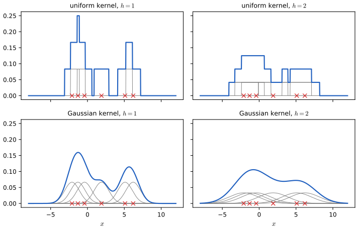
pp. 777–778 Density estimation evaluates \(p(x)\) for an observed vector: useful for outlier detection (Chapter 19), compression, generative classifiers and model comparison. In low dimension the simple kernel density estimator (Parzen window) works, \[ \hat p(x)=\frac1N\sum_{n=1}^NK_h(x-x_n),\qquad K_h(u)=\frac1hK(u/h),\ \ \int K=1,\ \int uK(u)\,\d u=0, \] with a bandwidth \(h\) controlling smoothness (Figure 20.5: a uniform kernel gives a staircase, a Gaussian kernel a smooth curve, and larger \(h\) smooths more). Since \(\hat p\) is a mixture of \(N\) equal-weight components centred at the data, it integrates to one and is the simplest "model" that memorises its training set; as \(h\to0\) it becomes a sum of delta functions with a perfect training fit and a useless held-out likelihood, a point the demonstration makes concrete. In high dimension a kernel estimator suffers from the curse of dimensionality (the required sample size grows exponentially in \(D\)), and a parametric density \(p_\theta(x)\) is needed. The bias–variance analysis of \(h\) is in Nonparametric Statistical Inference, 6.3 and All of Statistics, 20.3.
20.3.3 Imputation
pp. 778–779 For a data matrix \(X\) with observed part \(X_o\) and missing part \(X_m\), mean imputation fills each gap with the column mean \(\E[x_d]\), which ignores the dependencies between variables and gives no uncertainty (Figure 20.6). Multiple imputation fits a generative model to \(X_o\) (by EM, Chapter 6) and draws samples from \(p(X_m\given X_o)\); the same idea fills in occluded pixels of an image (inpainting). A general treatment of missing data is in Chapter 3.
20.3.4 Latent structure discovery
pp. 779–780 If \(z\) is read as the cause of \(x\), Bayes' rule inverts the model, \(p(z\given x)\propto p(z)p(x\given z)\), to find low-dimensional patterns. In the book's example the latent \(z\) is the unknown signalling network of a cell, \(x\in\mathbb R^{11}\) the measured phosphorylation of 11 proteins under 6 interventions \(a\in\{0,1\}^6\), and \(p(z\given\mathcal D)\) is obtained by Bayesian structure learning (dynamic programming over graphs, Chapter 30); edges with posterior probability above 0.5 recover most of the known pathway (Figure 20.7). The chapter-level theme, discovery, continues in Chapter 27.
20.3.5 Latent space interpolation
pp. 780–781 With an encoder \(e\) and decoder \(d\), two inputs \(x_1,x_2\) have codes \(z_i=e(x_i)\), and the points \(z=\lambda z_1+(1-\lambda)z_2\), \(0\le\lambda\le1\), decode to \(x'=d(z)\) that blend the semantic features of both (the justification for a straight line being that the learned manifold is often nearly flat; curved interpolation is sometimes better). A \(\beta\)-VAE (Chapter 21) gives a smooth morph from a 7 to a 2 on MNIST and between faces on CelebA (Figures 20.8, 20.9).
20.3.6 Latent space arithmetic
pp. 781–782 Given a labelled attribute (sunglasses), let \(\bar z^+\) and \(\bar z^-\) be the mean codes of images with and without it and \(\Delta=\bar z^+-\bar z^-\) the offset. Decoding \(z+s\Delta\) adds the attribute for \(s>0\) and removes it for \(s<0\) (as with word2vec analogies); a side effect can be changes correlated with the attribute in the data (more youthful and feminine faces when removing sunglasses), a symptom of dataset bias (Figure 20.10).
20.3.7 Generative design
p. 782 Generative design uses a model to propose candidate objects, such as molecules, with desired properties: fit a VAE to unlabelled examples and then run Bayesian optimisation in its latent space (Chapter 21).
20.3.8 Model-based reinforcement learning
p. 782 Where data are expensive (robotics), a generative world model lets an agent plan and learn "in its head"; see Chapter 35.
20.3.9 Representation learning
p. 782 The latent factors \(z\) that generate \(x\) can be used as features for downstream supervised tasks, even if they are uninterpretable (Chapter 32).
20.3.10 Data compression
p. 782 A model that gives high probability to common vectors and low probability to rare ones compresses data: the optimal code length for \(x\) from a source \(p(x)\) is \(\ell(x)=-\log p(x)\) (Shannon; Chapter 5, gap 20.6).
Filling the gap 20.6: the optimal code length is \(-\log p(x)\) p. 782
Derivation
Encode symbols \(x\in\{1,\dots,m\}\) with a prefix-free binary code of lengths \(\ell_x\). Kraft's inequality: a prefix code exists iff \(\sum_x2^{-\ell_x}\le1\) (each codeword of length \(\ell\) occupies a fraction \(2^{-\ell}\) of the binary tree below the root, and prefix-freeness means these subtrees are disjoint). Lower bound. Define \(r_x=2^{-\ell_x}/\sum_j2^{-\ell_j}\), a probability vector. By Gibbs' inequality \(\KL(p\|r)\ge0\), \[ \E_p[\ell_x]=-\sum_xp_x\log_2 2^{-\ell_x}=-\sum_xp_x\log_2r_x-\log_2\sum_j2^{-\ell_j}\ \ge\ -\sum_xp_x\log_2p_x+0=H_2(p) \] (using \(\sum_j2^{-\ell_j}\le1\)), so no prefix code beats the entropy in bits. Attainability. Take \(\ell_x=\lceil-\log_2p_x\rceil\): then \(\sum2^{-\ell_x}\le\sum p_x=1\), so a prefix code exists, and \(-\log_2p_x\le\ell_x<-\log_2p_x+1\) gives \(H_2(p)\le\E\ell<H_2(p)+1\). With a model \(q\) in place of the truth \(p\) the expected length of the \(q\)-code is \(H_{\rm ce}(p,q)\) and the penalty for the wrong model is exactly \(\KL(p\|q)\) bits; so a better density model is a better compressor. (Example: \(p=(0.4,0.3,0.2,0.1)\) has \(H=1.846\) bits and the Shannon code has mean length \(2.400<H+1\).)
20.4 Evaluating generative models
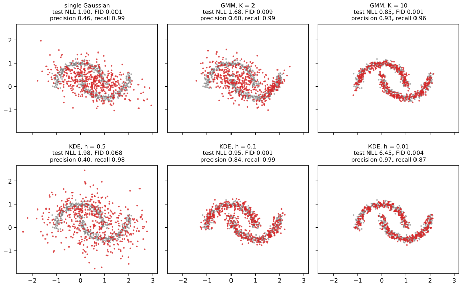
pp. 782–788 Evaluation must capture sample quality (do samples look like the data?), sample diversity (are all modes of the data covered?) and generalisation (beyond the training set?). No single metric does all three. A summary of what each score below can and cannot see, on one two-dimensional example, is the second of my figures.
20.4.1 Likelihood
pp. 783–785 The standard measure of closeness of a model \(q\) to the truth \(p\) is the KL divergence \[ \KL(p\|q)=-H(p)+H_{\rm ce}(p,q), \] where \(H(p)\) is a constant, so the cross entropy \(H_{\rm ce}(p,q)\) is what distinguishes models, and with the empirical distribution it is the (held-out) negative log-likelihood \(\frac1N\sum_n-\log q(x_n)\) (gap 20.1). For discrete data (language), this is easy to compute and is usually reported as perplexity \(2^{H}\), with \(H\) the cross entropy in bits per token. For images and audio the model is a continuous density and the data are discrete (e.g. \(x\in\{0,\dots,255\}^D\)), so the average log density can be arbitrarily large (a density may exceed one); the fix is uniform dequantisation: add \(u\sim U[0,1)^D\) to the data and model the continuous vector, which gives a lower bound on the log-likelihood of the discrete model (gap 20.2). Results are then reported in bits per dimension, \(\frac{\operatorname{NLL}}{D\ln2}\).
Filling the gap 20.1: KL, cross entropy, NLL, perplexity and bits per dimension pp. 783–784
Derivation
KL = cross entropy minus entropy. \(\KL(p\|q)=\int p\log\frac pq=\int p\log p-\int p\log q=-H(p)+H_{\rm ce}(p,q)\), where \(H(p)=-\int p\log p\) is finite for the cases of interest and does not depend on \(q\). So minimising \(\KL(p\|q_\theta)\) over \(\theta\) is minimising \(H_{\rm ce}(p,q_\theta)=-\E_p[\log q_\theta(x)]\). NLL estimates the cross entropy. If \(x_1,\dots,x_N\) are i.i.d. from \(p\), the sample average \(-\frac1N\sum_n\log q(x_n)\) is an unbiased estimator of \(H_{\rm ce}(p,q)\) for \(q\) fixed independently of the sample (strong law: it converges almost surely); on the training set it is optimistically biased for a fitted model, which is why the test-set NLL is reported. Minimising the training NLL is maximum likelihood, and \(\KL(\hat p_N\|q_\theta)\) with the empirical \(\hat p_N\) is minimised by the same \(\theta\).
Units. A cross entropy in nats is \(h\) with natural logarithms; in bits it is \(h/\ln2\) since \(\log_2t=\ln t/\ln2\). The perplexity \(2^{h/\ln2}=e^{h}\) is the same number whichever base is used, and equals the effective number of equally likely choices the model is torn between (a uniform model on \(m\) symbols has perplexity \(m\)). For a \(D\)-dimensional observation with total NLL \(h_{\rm tot}\) nats, bits per dimension \(=h_{\rm tot}/(D\ln2)\); e.g. 3.2 bits per dimension on a 784-pixel image is \(3.2\cdot784\cdot\ln2=1739\) nats. Both conversions were confirmed numerically.
Filling the gap 20.2: uniform dequantisation lower-bounds the discrete log-likelihood p. 784
Derivation
Let \(p(z)\) be a continuous density on \(\mathbb R^D\) and let a discrete observation be obtained by rounding down, \(x=\lfloor z\rfloor\) (one value per unit cell). The probability of \(x\) is \(P(x)=\int_{[x,x+1)}p(z)\,\d z\). Let \(q(z\given x)=\ind(z\in[x,x+1))\) be the uniform density on that cell (a probabilistic inverse of the rounding: it has support only where \(p(x\given z)=1\)). By Jensen's inequality for the concave \(\log\), \[ \log P(x)=\log\int q(z\given x)\frac{p(z)}{q(z\given x)}\,\d z\ \ge\ \int q(z\given x)\log\frac{p(z)}{q(z\given x)}\,\d z=\E_{u\sim U[0,1)^D}\big[\log p(x+u)\big], \] since \(q=1\) on the cell and \(\log q=0\). Therefore the average of the continuous log-density over the noise bounds the discrete log-likelihood from below; maximising the left side over the model also improves the discrete model, and the bound is tight in the limit of a density that is constant on cells. This is the book's statement (it phrases \(x\) as the rounding of a latent \(z\) and uses \(q(z\given x)\) as a variational distribution, the ELBO of the rounding model). Numerically, for a Gaussian \(p\) with standard deviation 2 and \(x\in\{-6,\dots,5\}\), the bound is below the exact log-probability for every \(x\) (largest gap 0.077).
20.4.1.2 Likelihood can be hard to compute
p. 785 For models with an intractable normaliser the likelihood is not available. Variational inference gives lower (sometimes upper) bounds (Chapter 10), annealed importance sampling gives Monte Carlo estimates (Chapter 11), and for implicit models such as GANs the likelihood is not even defined, so likelihood-free metrics are needed.
20.4.1.3 Likelihood is not related to sample quality
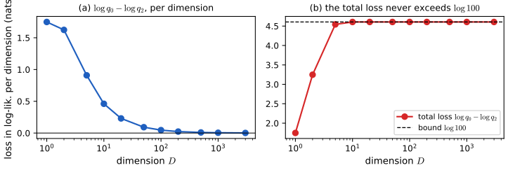
p. 785 A model can have excellent likelihood and bad samples, and conversely (Theis et al. 2016). (i) Let \(q_0\) be a very good density model and \(q_1\) white noise, and sample from \(q_2=0.01q_0+0.99q_1\): 99% of the samples are noise, yet \(\log q_2\) differs from \(\log q_0\) by at most \(\log100\) in total, which per dimension vanishes as \(D\) grows. (ii) Let \(q\) be a Gaussian mixture with one narrow component on each training image: its samples are the training images (they look perfect), but on test data its likelihood is dreadful, since the model has memorised (gap 20.3). The own figure below demonstrates (i), and the family comparison (ii).
Filling the gap 20.3: both halves of the likelihood-versus-quality argument p. 785
Derivation
(i) Good likelihood, bad samples. For any \(x\), \(q_2(x)=0.01q_0(x)+0.99q_1(x)\ge0.01q_0(x)\) since \(q_1\ge0\), hence \(\log q_2(x)\ge\log q_0(x)-\log100\), i.e. \(\log q_0(x)-\log q_2(x)\le\log100=4.605\) for every \(x\), not just on average, and this is also approximately attained when \(q_0(x)\gg q_1(x)\) (then \(q_2\approx0.01q_0\)). On data of dimension \(D\), \(|\log q_0(x)|\) typically scales like \(D\) (it is a sum over coordinates), so the relative change in log-likelihood, \(\le\log100/|\log q_0|\), goes to zero as \(D\) grows; the reported log-likelihood per dimension changes by at most \(4.605/D\) nats. Yet 99% of the samples of \(q_2\) are drawn from the noise model. In the own figure (\(q_0=\mathcal N(0,0.1^2I)\), \(q_1=\mathcal N(0,I)\)) the average loss is \(4.605\) nats in total for large \(D\), exactly at the bound, and \(4.6/D\) nats per dimension.
(ii) Good samples, bad likelihood. Let \(q(x)=\frac1N\sum_n\mathcal N(x\given x_n,\epsilon^2I)\) with training points \(x_n\). Sampling picks a training point and adds noise of scale \(\epsilon\), imperceptible for small \(\epsilon\), so samples look like real data. For a test point \(x^\circ\) at distance \(d_n\) from training point \(x_n\), \(q(x^\circ)\le\max_n\mathcal N(x^\circ\given x_n,\epsilon^2I)=(2\pi\epsilon^2)^{-D/2}\exp(-d_{\min}^2/(2\epsilon^2))\), so \(\log q(x^\circ)\le-\frac D2\log(2\pi\epsilon^2)-\frac{d_{\min}^2}{2\epsilon^2}\to-\infty\) as \(\epsilon\to0\) whenever \(d_{\min}>0\), i.e. whenever the test point is not a copy of a training point. The held-out likelihood diverges to \(-\infty\) while the training likelihood diverges to \(+\infty\): overfitting. The two-moons demonstration shows this with a kernel estimator of bandwidth \(0.01\): test NLL 6.5 against 0.95 for bandwidth 0.1.
20.4.2 Distances and divergences in feature space
pp. 785–787 Comparing high-dimensional distributions in pixel space is hopeless, so metrics map samples to the features of a (usually pretrained) classifier and compare the feature distributions. The Inception score (Salimans et al. 2016) is \(\exp\{\E_{p_\theta(x)}\KL(p_{\rm disc}(y\given x)\|p_\theta(y))\}\) with \(p_\theta(y)=\int p_{\rm disc}(y\given x)p_\theta(x)\,\d x\), and satisfies \(\log\mathrm{IS}=H(p_\theta(y))-\E_{p_\theta(x)}H(p_{\rm disc}(y\given x))\): a high score needs samples that are individually easy to classify (low conditional entropy) and collectively spread over classes (high marginal entropy). It sees only the class labels, so a model that outputs one perfect image per class gets a perfect score (gap 20.4). The Fréchet Inception distance (FID; Heusel et al. 2017) fits a Gaussian to the features of model samples (\(\mu_m,\Sigma_m\)) and one to the data (\(\mu_d,\Sigma_d\)) and takes the Fréchet distance \[ \operatorname{FID}=\|\mu_m-\mu_d\|^2+\operatorname{tr}\big(\Sigma_m+\Sigma_d-2(\Sigma_m\Sigma_d)^{1/2}\big), \] lower is better (gap 20.5). Because it uses features rather than logits, it captures more than the class structure, but it has a high bias that depends on the number of samples; the kernel Inception distance (Bińkowski et al. 2018) instead uses the squared maximum mean discrepancy between feature sets, which has an unbiased estimator.
Filling the gap 20.4: the Inception score is the exponential of a mutual information, between 1 and the number of classes p. 786
Derivation
Let \(x\sim p_\theta\) and let \(y\) be drawn from \(p_{\rm disc}(y\given x)\); the marginal of \(y\) is \(p_\theta(y)\), so \((x,y)\) has joint \(p_\theta(x)p_{\rm disc}(y\given x)\). Then \[ \E_{p_\theta(x)}\KL\big(p_{\rm disc}(y\given x)\|p_\theta(y)\big)=\E\Big[\sum_yp_{\rm disc}(y\given x)\log\frac{p_{\rm disc}(y\given x)}{p_\theta(y)}\Big]=I(x;y), \] the mutual information (the KL between the joint and the product of marginals). Expanding the logarithm, \(\sum_yp(y\given x)\log p(y\given x)-\sum_yp(y\given x)\log p_\theta(y)\) and averaging over \(x\): the first part is \(-\E_xH(p(y\given x))\) and the second, since \(\E_xp(y\given x)=p_\theta(y)\), is \(+H(p_\theta(y))\). So \(\log\mathrm{IS}=I(x;y)=H(y)-H(y\given x)\), as the book states. Bounds: \(I\ge0\) (nonnegativity of KL) so \(\mathrm{IS}\ge1\), with equality iff \(y\) is independent of \(x\); \(H(y\given x)\ge0\) and \(H(y)\le\log C\) give \(I\le\log C\), so \(\mathrm{IS}\le C\), with equality iff every sample is classified with certainty and the classes are balanced. The score is therefore capped at the number of classes and blind to everything inside a class: one perfect example per class already achieves \(C\). Confirmed numerically (random classifier outputs: identity to \(10^{-10}\); confident balanced outputs: \(\mathrm{IS}\approx C\)).
Filling the gap 20.5: the Fréchet distance is the 2-Wasserstein distance between the two Gaussians p. 787
Derivation
The book defines FID by its formula; the reason it is a distance between distributions is that \[ \operatorname{FID}=W_2^2\big(\mathcal N(\mu_m,\Sigma_m),\mathcal N(\mu_d,\Sigma_d)\big)=\min_{\text{couplings}}\E\|X-Y\|^2. \] Reduction to covariances. For any coupling \((X,Y)\), \(\E\|X-Y\|^2=\|\mu_1-\mu_2\|^2+\operatorname{tr}\Sigma_1+\operatorname{tr}\Sigma_2-2\operatorname{tr}C\) where \(C=\operatorname{Cov}(X,Y)\), so the problem is to maximise \(\operatorname{tr}C\). It is a standard fact (Dowson and Landau 1982; Olkin and Pukelsheim 1982) that the optimal coupling of two Gaussians is jointly Gaussian, so we need only the cross-covariances \(C\) for which \(\begin{pmatrix}\Sigma_1&C\\C^\T&\Sigma_2\end{pmatrix}\succeq0\). Maximisation. Assume \(\Sigma_1,\Sigma_2\succ0\). Positive semidefiniteness of the block matrix is equivalent to \(C=\Sigma_1^{1/2}K\Sigma_2^{1/2}\) with \(\|K\|_{\rm op}\le1\) (a Schur-complement argument). Then \(\operatorname{tr}C=\operatorname{tr}(K\,\Sigma_2^{1/2}\Sigma_1^{1/2})\le\|\Sigma_2^{1/2}\Sigma_1^{1/2}\|_{*}\), the nuclear norm (von Neumann's trace inequality, \(|\operatorname{tr}(KM)|\le\|K\|_{\rm op}\|M\|_*\)), with equality for \(K\) the polar factor of \(\Sigma_1^{1/2}\Sigma_2^{1/2}\). The nuclear norm is the sum of singular values of \(\Sigma_2^{1/2}\Sigma_1^{1/2}\), i.e. \(\operatorname{tr}\big((\Sigma_1^{1/2}\Sigma_2\Sigma_1^{1/2})^{1/2}\big)\). Finally, \(\Sigma_1^{1/2}\Sigma_2\Sigma_1^{1/2}\) and \(\Sigma_1\Sigma_2\) are similar matrices (conjugate by \(\Sigma_1^{1/2}\)), so they have the same eigenvalues and the same trace of square root: \(\operatorname{tr}(\Sigma_1\Sigma_2)^{1/2}\). Hence \[ W_2^2=\|\mu_1-\mu_2\|^2+\operatorname{tr}\big(\Sigma_1+\Sigma_2-2(\Sigma_1\Sigma_2)^{1/2}\big). \] One dimension: \(\operatorname{FID}=(\mu_1-\mu_2)^2+(\sigma_1-\sigma_2)^2\), since \(\operatorname{tr}\Sigma_i=\sigma_i^2\) and \(2\sqrt{\sigma_1^2\sigma_2^2}=2\sigma_1\sigma_2\); e.g. \(\mathcal N(0,1)\) against \(\mathcal N(1,4)\): \(1+1=2\). The distance is symmetric, zero iff the Gaussians coincide, and, as the next figure shows, it depends on the data only through the first two moments of the features: two clouds with the same mean and covariance have \(\operatorname{FID}=0\) whatever their shape. Checked numerically against an eigenvalue formula and a matrix square root.
20.4.3 Precision and recall metrics
pp. 787–788 A single distance cannot tell whether a bad score means poor samples or poor coverage. The remedy (Kynkäänniemi et al. 2019) is a pair of metrics from nearest neighbours in feature space. For a set \(\Phi\) of feature vectors and a point \(\phi'\) let \(\operatorname{NN}_k(\phi',\Phi)\) be its \(k\)-th nearest neighbour in \(\Phi\), and define the manifold \(\operatorname{supp}(\Phi)=\bigcup_{\phi\in\Phi}B(\phi,\|\phi-\operatorname{NN}_k(\phi,\Phi)\|)\), the union of balls around each point reaching its \(k\)-th neighbour. Precision is the fraction of model samples that fall in the data manifold (are samples as close to the data as data are to each other?) and recall the fraction of data points in the model manifold (is the data as close to samples as samples are to each other?). Both lie in \([0,1]\) (precision \(=\) recall \(=1\) when the two sets coincide), the parameter \(k\) controls leniency (larger \(k\), larger values), and sweeping a model parameter gives a precision–recall curve for choosing among models. They diagnose mode collapse (high precision, low recall) in GANs (Chapter 26).
20.4.4 Statistical tests
pp. 788–789 A two-sample test asks whether model samples and data come from the same distribution: the null hypothesis is equality, a statistic is compared with a threshold, and the user fixes the type I error rate. Statistics based on classifiers (a classifier that cannot beat chance on held-out samples is evidence for the null) or on the maximum mean discrepancy have been used for implicit models, with learned features in high dimension. They give a calibrated decision, but are too expensive to monitor training; they suit comparison of fully trained models.
20.4.5 Challenges with using pretrained classifiers
p. 789 IS, FID, nearest-neighbour metrics and feature-space tests all rely on a pretrained classifier. Its features may transfer poorly to a dataset it was not trained for; and if it was trained on the same data, the generated samples that are imperfect are out of distribution for it, so its features are unreliable exactly where it matters. These concerns are not only theoretical (Rosca et al.; Barratt and Sharma 2018).
| Model | test NLL | FID | precision | recall |
|---|---|---|---|---|
| single Gaussian | 1.90 | 0.0014 | 0.46 | 0.99 |
| mixture, K = 2 | 1.68 | 0.0087 | 0.60 | 0.99 |
| mixture, K = 10 | 0.85 | 0.0014 | 0.93 | 0.96 |
| kernel, h = 0.5 | 1.98 | 0.068 | 0.40 | 0.98 |
| kernel, h = 0.1 | 0.95 | 0.0008 | 0.84 | 0.99 |
| kernel, h = 0.01 | 6.45 | 0.0042 | 0.97 | 0.87 |
Reading the table: the likelihood penalises the memoriser and the diffuse model but not a misshapen one with the right spread; the Fréchet distance (here on raw coordinates, standing in for features) is blind to shape; precision and recall separate the misshapen models (low precision) from the memoriser (lower recall, because held-out points are not near a copy of the training data when the balls are tiny).
Supplement S20 (Generative models: an overview)
The supplement's Chapter 20 consists of the chapter title only; there is no additional material for this chapter in the draft.
Practice problems
The book has no exercises for this chapter. These three short problems are my own.
Practice problem 20.1 (bits per dimension). An image model reaches 2.9 bits per dimension on \(32\times32\) colour images. What is the average code length per image in bits, and the NLL in nats? What perplexity per dimension is that?
Solution
\(D=32\cdot32\cdot3=3072\). Bits per image \(=2.9\cdot3072=8909\). In nats, \(8909\cdot\ln2=6175\). Per dimension the cross entropy is \(2.9\) bits, so the perplexity is \(2^{2.9}=7.46\): the model is as uncertain about each sub-pixel value as a uniform choice among about 7.5 of the 256 values (before the dequantisation correction).
Practice problem 20.2 (a perfect Inception score). A classifier has \(C=10\) classes and a generator produces exactly one fixed image per class, each classified with certainty. What is the Inception score and the FID-type failure it hides?
Solution
\(p_{\rm disc}(y\given x)\) is one-hot, so \(H(y\given x)=0\); the generator picks each class with probability \(1/10\), so \(H(p_\theta(y))=\log10\). Then \(\log\mathrm{IS}=\log10\) and \(\mathrm{IS}=10\), the maximum (gap 20.4). It hides mode collapse within classes: the model has only ten distinct outputs, so recall is near zero (almost no real image lies in the balls around the ten samples) and any feature-space distance such as FID would be large.
Practice problem 20.3 (an FID by hand). Features of the data are \(\mathcal N(0,1)\) and features of the model samples \(\mathcal N(1,4)\) in one dimension. Give the FID, and say what changes if the model's variance is 1.
Solution
In one dimension \(\operatorname{FID}=(\mu_m-\mu_d)^2+(\sigma_m-\sigma_d)^2=(1-0)^2+(2-1)^2=2\), where the second term uses the standard deviations \(\sigma_m=2\), \(\sigma_d=1\). With variance 1 the second term vanishes and \(\operatorname{FID}=1\); with equal means as well it is 0 even if the model's samples are not Gaussian at all (gap 20.5).
Demonstration
| Page | What it shows | In the notes |
|---|---|---|
| Judging a generative model | Two-moons or three-cluster data; a Gaussian, a Gaussian mixture (1–12 components) or a kernel estimator (bandwidth 0.01–2); samples, density shading, held-out NLL, Fréchet distance, precision and recall. Presets: 1 a good mixture; 2 a single Gaussian (FID near zero); 3 a memoriser; 4 oversmoothing; 5 two components; 6 the right model for three clusters. | Section 20.4 |
The Python code that produces every figure of this page is code/ch20_generative_models_overview.py (see the code index). Companion demos: change of variables.
Notes on the book
A point where the book is imprecise
- Section 20.2, sampling speed of flows. The text groups normalising flows with the slow samplers. For a flow \(x=f^{-1}(z)\) with coupling layers, sampling takes a single pass through the inverse, about as costly as evaluating the density; flows with autoregressive layers are fast in one direction and sequential in the other. "Slow" is correct for autoregressive models, diffusion models and MCMC-sampled energy-based models, but for flows it depends on the architecture (the table above says so).
References
- Murphy, K. P. (2023). Probabilistic Machine Learning: Advanced Topics. MIT Press, Cambridge, MA. Chapter 20, pp. 773–790. probml.github.io/pml-book/book2.html.
- Bińkowski, M., Sutherland, D. J., Arbel, M. and Gretton, A. (2018). Demystifying MMD GANs. International Conference on Learning Representations.
- Dowson, D. C. and Landau, B. V. (1982). The Fréchet distance between multivariate normal distributions. Journal of Multivariate Analysis, 12(3), 450–455.
- Heusel, M., Ramsauer, H., Unterthiner, T., Nessler, B. and Hochreiter, S. (2017). GANs trained by a two time-scale update rule converge to a local Nash equilibrium. Advances in Neural Information Processing Systems, 30.
- Kynkäänniemi, T., Karras, T., Laine, S., Lehtinen, J. and Aila, T. (2019). Improved precision and recall metric for assessing generative models. Advances in Neural Information Processing Systems, 32.
- Olkin, I. and Pukelsheim, F. (1982). The distance between two random vectors with given dispersion matrices. Linear Algebra and its Applications, 48, 257–263.
- Salimans, T., Goodfellow, I., Zaremba, W., Cheung, V., Radford, A. and Chen, X. (2016). Improved techniques for training GANs. Advances in Neural Information Processing Systems, 29.
- Shannon, C. E. (1948). A mathematical theory of communication. Bell System Technical Journal, 27, 379–423 and 623–656.
- Theis, L., van den Oord, A. and Bethge, M. (2016). A note on the evaluation of generative models. International Conference on Learning Representations.
The numerical statements in the text (KDE normalisation and agreement with a library estimator, monotone EM, the Gaussian mixture against a library fit, the bits-per-dimension and perplexity conversions, the dequantisation bound, the mixture bound on the log-likelihood, the Inception-score identity and its maximum, the Fréchet distance in one and two dimensions, precision and recall on identical and disjoint sets, Shannon code lengths, the behaviour of the six models on the two-moons data and the interactive demonstration) were confirmed numerically.