Discovery methods: an overview
Prediction and generation are not enough when the goal is to understand a data set. This chapter opens Part V with the idea of discovery by latent-variable modelling: the observation is generated by interpretable hidden factors, the map from factors to observations is often many-to-one so that the inverse problem is ill-posed, and a prior makes the answer well defined. The notes expand the two-page introduction with a worked linear-Gaussian version in which every claim can be checked, and map the chapters of Part V (latent factor, state-space, graph, nonparametric, representation learning and interpretability) onto this course.
Ch. 1 Introduction Ch. 2 Probability Ch. 3 Statistics Ch. 4 Graphical models Ch. 5 Information theory Ch. 6 Optimisation Ch. 7 Inference algorithms Ch. 8 Gaussian filtering Ch. 9 Message passing Ch. 10 Variational inference Ch. 11 Monte Carlo Ch. 12 MCMC Ch. 13 Sequential Monte Carlo Ch. 14 Predictive models Ch. 15 GLMs Ch. 16 Deep networks Ch. 17 Bayesian neural networks Ch. 18 Gaussian processes Ch. 19 Beyond iid Ch. 20 Generative models Ch. 21 VAEs Ch. 22 Autoregressive models Ch. 23 Normalizing flows Ch. 24 Energy-based models Ch. 25 Diffusion models Ch. 26 GANs Ch. 27 Discovery methods Ch. 28 Latent factor models Ch. 29 State-space models Ch. 30 Graph learning Ch. 31 Nonparametric Bayes Ch. 32 Representation learning Ch. 33 Interpretability Ch. 34 Decision making Ch. 35 Reinforcement learning Ch. 36 Causality
How to read these notes
They follow the book. Sections carry the book's numbers and the one numbered equation keeps its number, (27.1). This chapter opens Part V, on discovery, with a two-page introduction and a map of the chapters that follow. The notes expand the map, link forward to the chapters of this course, and prove the statement the book makes about the inverse problem in a case where everything is explicit (a linear-Gaussian model).
Filling the gaps. Orange Filling the gap boxes give the full argument for the statements about inverse problems and the MAP estimate (27.1). Proofs start hidden.
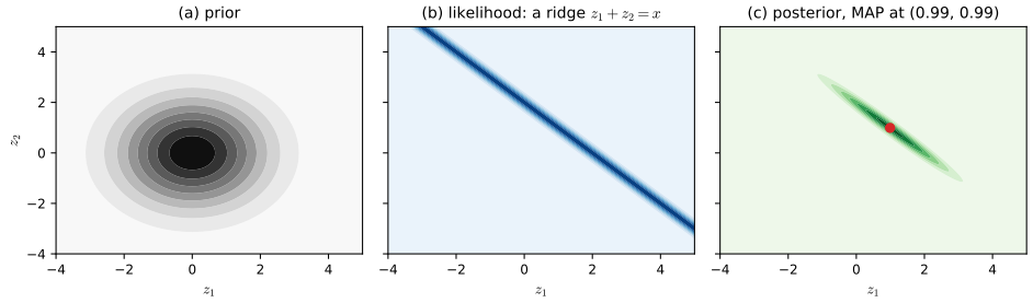
Figures. Figure 27.1 in the book (vision as inverse graphics) is a drawing and is not reproduced; one figure of my own, computed, illustrates the linear-Gaussian version.
Main reference
K. P. Murphy, Probabilistic Machine Learning: Advanced Topics, MIT Press (2023; December 2025 draft), Chapter 27, pages 927–928 (book page: probml.github.io/pml-book/book2.html). The explanations, derivations, figure and code are my own.
Companion courses
- Probabilistic Machine Learning: An Introduction: Chapter 20 dimensionality reduction (PCA, factor analysis, autoencoders), 21.4 clustering with mixture models.
- Bayesian and Probabilistic Machine Learning: Chapter 12 continuous latent variables, Chapter 9 mixture models and EM, Chapter 13 sequential data.
- Nonparametric Statistical Inference: Chapter 10 (Dirichlet process and other topics); Foundations of Deep Learning: Chapter 16 continuous latent variables.
27.1 Introduction
p. 927 Parts III and IV showed how to build models that predict outputs from inputs (supervised learning: maximise a conditional likelihood) and models that generate outputs unconditionally (unsupervised learning: maximise an unconditional likelihood). Sometimes the goal is neither but to understand a data set: to discover something interesting and possibly actionable. Prediction and generation are useful subroutines for discovery but are not sufficient: neural networks often learn useful features implicitly, yet these are hard to interpret, and can be unstable, depending on arbitrary details such as the learning rate or the random seed.
The approach of this Part is to learn models with an interpretable representation of high-dimensional data. The usual device is a latent variable model: the observed \(x\) was caused or generated by underlying, usually low-dimensional, latent factors \(z\), which represent the true state of the world and, crucially, are meaningful to the model's user (so evaluating such models usually needs domain expertise). Take the interpretation of an image \(x\) in terms of a 3-d scene \(z\) (objects and surfaces). The forward map \(z\mapsto x\) is often many-to-one, because different scenes \(z\ne z'\) can give the same image through the limitations of the sensor (perceptual aliasing), so the inverse map \(x\mapsto z\) is ill-posed, and a prior \(p(z)\) is needed to make the estimate well defined. In simple settings a point estimate is enough, the MAP estimate \[ \hat z(x)=\argmax_z\,p(z\given x)=\argmax_z\ \big[\log p(z)+\log p(x\given z)\big]. \tag{27.1} \] In computer vision this is "vision as inverse graphics" or analysis by synthesis (Figure 27.1 in the book): the agent infers the scene by finding the scene whose rendering best matches the image, weighted by the prior. The same inverse-modelling idea is used throughout science and engineering, where \(z\) is a state of the world and \(x\) a noisy or partial manifestation. Sometimes the prior \(p(z\given\theta)\) and the likelihood \(p(x\given z,\theta)\) are fully known and only the inference for \(z\) remains; more often the parameters \(\theta\) are partly unknown and must be learned from samples \(\mathcal D=\{x_n\}_{n=1}^N\), and sometimes even the structure of the model is unknown and must be learned too (Chapter 30). The inference algorithms are those of Chapter 7; the example of Section 1.2 is the scalar case of aliasing.
Filling the gap 27.1: when two causes give the same data, the posterior odds are the prior odds p. 927
Derivation
Suppose the likelihood cannot distinguish two latent values, \(p(x\given z,\theta)=p(x\given z',\theta)\) (for instance \(x=f(z)+\varepsilon\) with \(f(z)=f(z')\) and noise of the same law). Then Bayes' rule gives \[ \frac{p(z\given x)}{p(z'\given x)}=\frac{p(x\given z)p(z)/p(x)}{p(x\given z')p(z')/p(x)}=\frac{p(z)}{p(z')}, \] because the evidence \(p(x)\) is common and the likelihoods cancel. So the data carry no information about which of the two is the cause, and any preference must come from the prior. More generally, if \(f(z)=f(z')\) on a whole set \(\mathcal Z_x\) (a fibre of \(f\)), the posterior restricted to the fibre is proportional to the prior restricted to it. When the fibre is a continuum (\(f\) not injective on a manifold of directions), the likelihood is flat along it, the maximum-likelihood estimate is not unique (the model is not identifiable from \(x\)), and a prior is what selects a point: this is why the MAP (27.1) is well defined when the ML estimate is not, and also why conclusions about aliased directions are driven entirely by assumptions (the prior), not by data.
Filling the gap 27.2: the linear-Gaussian inverse problem; MAP is a ridge solution p. 927, (27.1)
Derivation
Take the linear "renderer" \(x=\bm Az+\varepsilon\), \(\varepsilon\sim\mathcal N(0,\sigma^2\bm I)\), with prior \(z\sim\mathcal N(\bm m_0,\tau^2\bm I)\) in \(\mathbb R^d\). Then \[ \log p(z\given x)=-\frac1{2\sigma^2}\|x-\bm Az\|^2-\frac1{2\tau^2}\|z-\bm m_0\|^2+\const. \] Collect the terms quadratic and linear in \(z\) (completing the square): \(-\frac12z^\T\bm Pz+z^\T\bm b+\const\) with precision \(\bm P=\bm A^\T\bm A/\sigma^2+\bm I/\tau^2\) and \(\bm b=\bm A^\T x/\sigma^2+\bm m_0/\tau^2\). Since \(\bm P\succ0\) (the second term is positive definite even if \(\bm A\) is rank deficient), the posterior is Gaussian, \[ p(z\given x)=\mathcal N(\bm P^{-1}\bm b,\ \bm P^{-1}), \] and its mean equals its mode, so the MAP estimate (27.1) is \(\hat z=\bm P^{-1}\bm b\). Multiplying \(\bm P\hat z=\bm b\) by \(\sigma^2\): \(\hat z=\argmin_z\ \|x-\bm Az\|^2+\lambda\|z-\bm m_0\|^2\) with \(\lambda=\sigma^2/\tau^2\): a ridge (Tikhonov) regression towards the prior mean. Aliasing in this model. If \(\bm A\bm v=0\) for a unit vector \(\bm v\) (a latent direction the sensor cannot see), then \(\bm v^\T\bm P\bm v=1/\tau^2\), and \(\bm v\) is an eigenvector of \(\bm P\) (because \(\bm A^\T\bm A\bm v=0\)), so the posterior variance in the direction \(\bm v\) is exactly the prior variance \(\tau^2\), and with \(\bm m_0=0\) the MAP has no component along it, \(\bm v^\T\hat z=0\). In the visible directions the posterior variance is \(1/(\mu/\sigma^2+1/\tau^2)\) for each singular value \(\mu\) of \(\bm A^\T\bm A\). In the figure below \(\bm A=(1\ 1)\), \(\sigma=0.2\), \(\tau=1.5\), \(x=2\): along \((1,-1)/\sqrt2\) the posterior variance is \(2.25\) (the prior's), along \((1,1)/\sqrt2\) it is \(1/(2/0.04+1/2.25)=0.0198\), and the MAP is \((0.991,0.991)\). These match a brute-force grid posterior to three decimals.
27.2 Overview of Part V
p. 928 The chapters of Part V, and where each is in this course:
- Chapter 28, latent factor models: simple latent-variable models for fixed-dimensional vectors \(x\in\mathbb R^D\): mixtures, factor analysis, probabilistic PCA and relatives (companion: PML 20, ML 12).
- Chapter 29, state-space models: the same ideas for sequences of correlated vectors \(x_{1:T}\) (speech, video, genomics), with nonlinear ("deep") extensions and spatio-temporal versions (companion: ML 13).
- Chapter 30, graph learning: extension to general graphs, including learning the graph itself (mostly in the supplement).
- Chapter 31, nonparametric Bayesian models: represent uncertainty about the number of hidden states, the structure or the form of a functional dependency, so that the complexity of the learned representation grows with the data's quantity and informativeness; important for discovery, and keeps flexibility while retaining interpretability (mostly in the supplement; companion: NPS 10).
- Chapter 32, representation learning with neural networks, by latent-variable modelling and by other estimation methods (companion: PML 19).
- Chapter 33, interpretability: how to explain the behaviour of a predictive model, typically a neural network.
After discovery the book turns to decisions under uncertainty, Chapter 34, Chapter 35 and, finally, Chapter 36 (causality), which is where the questions "what caused this?" and "what if I act?" meet.
Supplement S27 (Discovery methods: an overview)
The supplement's Chapter 27 consists of the chapter title only; there is no additional material for this chapter in the draft.
Practice problems
The book has no exercises for this chapter. These two short problems are my own.
Practice problem 27.1 (the ridge solution). For \(\bm A=(1\ \ 1)\), \(\sigma=0.2\), \(\tau=1.5\), \(\bm m_0=0\) and \(x=2\), find the MAP estimate in closed form.
Solution
The ridge solution is \(\hat z=\bm A^\T(\bm A\bm A^\T+\lambda\bm I)^{-1}x\) with \(\lambda=\sigma^2/\tau^2=0.04/2.25=0.01778\) (push-through identity: \((\bm A^\T\bm A+\lambda\bm I)^{-1}\bm A^\T=\bm A^\T(\bm A\bm A^\T+\lambda\bm I)^{-1}\)). Here \(\bm A\bm A^\T=2\), so \(\hat z=(1,1)^\T\cdot2/(2+0.01778)=(0.9912,0.9912)^\T\). The two coordinates are equal because nothing in the data or the prior distinguishes them; their sum \(1.982\) is slightly shrunk below the observation 2 by the prior.
Practice problem 27.2 (what the data cannot say). In the same model, how much does observing \(x\) change the variance of \(z_1-z_2\)? And of \(z_1+z_2\)?
Solution
Write \(u=(z_1-z_2)/\sqrt2\) (invisible direction) and \(v=(z_1+z_2)/\sqrt2\) (visible). A priori \(\operatorname{var}u=\operatorname{var}v=\tau^2=2.25\) and they are independent. The data measure \(v\) only, \(x=\sqrt2\,v+\varepsilon\), so \(\operatorname{var}(u\given x)=2.25\): unchanged (gap 27.2). For \(v\), the precision rises from \(1/2.25\) to \(2/\sigma^2+1/\tau^2=50+0.444\), so \(\operatorname{var}(v\given x)=0.0198\): a reduction by a factor of about 114. Since \(z_1-z_2=\sqrt2\,u\) and \(z_1+z_2=\sqrt2\,v\), the variances of those combinations are \(2\cdot2.25=4.5\) (unchanged) and \(2\cdot0.0198=0.0396\).
Notes on the book
No errors found
This chapter is an introduction and a map; it contains one equation, (27.1), which is the standard MAP rule and is correct as stated, and nothing that needs correcting.
References
- Murphy, K. P. (2023). Probabilistic Machine Learning: Advanced Topics. MIT Press, Cambridge, MA. Chapter 27, pp. 927–928. probml.github.io/pml-book/book2.html.
- Hadamard, J. (1902). Sur les problèmes aux dérivées partielles et leur signification physique. Princeton University Bulletin, 13, 49–52.
- Tikhonov, A. N. (1963). On the solution of ill-posed problems and the method of regularization. Doklady Akademii Nauk SSSR, 151, 501–504.
- Yuille, A. and Kersten, D. (2006). Vision as Bayesian inference: analysis by synthesis? Trends in Cognitive Sciences, 10(7), 301–308.
The numerical statements in the text (the closed-form Gaussian posterior against a brute-force grid, the MAP as the ridge solution, the unchanged posterior variance along the direction the sensor cannot see and the variance along the visible one) were confirmed numerically.