Logistic Regression
Logistic regression models the probability of a class label as a sigmoid (two classes) or softmax (many classes) of a linear function of the inputs. Fitting it by maximum likelihood is a convex problem with a gradient that is simply "error times input" and a Hessian that is a weighted Gram matrix, which makes every first- and second-order optimiser of Chapter 8 applicable: stochastic gradient descent, Newton's method in its guise as iteratively reweighted least squares, and the bound-optimisation iteration with a fixed curvature matrix. The chapter then adds a prior (weight decay), maximum-entropy features, robustness to label noise through a mixture likelihood and the bi-tempered loss, and a Bayesian treatment with the Laplace approximation and the probit predictive. The notes prove every statement the book leaves as "one can show" or as an exercise, and test the claims on the iris data and on small simulated problems.
Ch. 1 Introduction Ch. 2 Univariate probability Ch. 3 Multivariate probability Ch. 4 Statistics Ch. 5 Decision theory Ch. 6 Information theory Ch. 7 Linear algebra Ch. 8 Optimisation Ch. 9 Discriminant analysis Ch. 10 Logistic regression Ch. 11 Linear regression Ch. 12 GLMs Ch. 13 Networks for tabular data Ch. 14 Networks for images Ch. 15 Networks for sequences Ch. 16 Exemplar-based methods Ch. 17 Kernel methods Ch. 18 Trees and boosting Ch. 19 Fewer labels Ch. 20 Dimensionality reduction Ch. 21 Clustering Ch. 22 Recommender systems Ch. 23 Graph embeddings
How to read these notes
They follow the book. Sections carry the book's numbers (10.2.3, 10.3.4, ...) and equations the book numbers keep their numbers, e.g. \((10.23)\); equations without a number are steps the book skips. The book marks Sections 10.4 and 10.5 as optional (stars); they are covered in full here.
Filling the gaps. Wherever the book writes "one can show", leaves a step to an exercise, or quotes a result from the literature, an orange Filling the gap box gives the full argument. Proofs start hidden: open one with its bar, or use the buttons below.
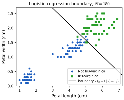
Figures and demonstrations. Every computed figure is reproduced by the Python code; Figures 10.1a, 10.8, 10.9 and 10.15 are hand-drawn sketches and are not reproduced. Data: Figures 10.1b and 10.5 use the iris measurements; Figures 10.4, 10.6, 10.7, 10.12, 10.13 and 10.14 use small simulated data sets because the book's own point sets are not available offline, and Figure 10.10 follows the recipe in the text on the iris data; the captions say so. The ▶ Demo boxes open an interactive demonstration set to the case being discussed.
Main reference
K. P. Murphy, Probabilistic Machine Learning: An Introduction, MIT Press (2022), Chapter 10, pages 339–369 (book page: probml.github.io/pml-book/book1.html). Section, equation, figure and exercise numbers below refer to this book. The explanations, derivations, figures and code are my own.
Companion courses
Logistic regression is also developed, in other notation, elsewhere on this site. Where a result is proved in full there, these notes give the statement and a short sketch and link to it.
- Bayesian and Probabilistic Machine Learning (Bishop): 4.1.7 the perceptron, 4.3.2 logistic regression, 4.3.3 iterative reweighted least squares, 4.3.4 multiclass logistic regression, 4.3.6 canonical link functions, 4.4 the Laplace approximation, 4.5.1 and 4.5.2 Bayesian logistic regression and its predictive distribution.
- Elements of Statistical Learning (Hastie, Tibshirani, Friedman): 4.4 logistic regression and 4.4.1 fitting by Newton-Raphson, 4.4.4 L1-regularised logistic regression.
- Introduction to Statistical Learning: 4.3 logistic regression and 4.3.5 multinomial logistic regression.
- Foundations of Deep Learning (Bishop and Bishop): Chapter 5 on single-layer classification (cross entropy, softmax, the same gradient).
- All of Statistics: Chapter 13 on regression (logistic regression as a generalised linear model).
What this chapter adds: separability and the non-existence of the MLE, the perceptron mistake bound, the fixed-matrix bound optimisation iteration, the identifiability argument for the penalised softmax, maximum-entropy classifiers, hierarchical softmax and long-tail sampling, the mixture and bi-tempered robust losses, and the probit predictive with its multiclass generalisation.
The chapter at a glance
- 10.2.1–10.2.2 The model \(p(y=1\given\bm x)=\sigma(\bm w^\T\bm x+b)\) has a linear boundary; a feature map \(\bm\phi\) makes it nonlinear (gap 10.1).
- 10.2.3 Gradient \(\frac1N\sum_n(\mu_n-y_n)\bm x_n\) and Hessian \(\frac1N\bm X^\T\bm S\bm X\) (gap 10.3); the NLL is convex but the MLE exists only for non-separable data (Result 10.1).
- 10.2.4–10.2.6 SGD and its rate (gap 10.4), the perceptron and its mistake bound (gap 10.5), Newton's method as IRLS and why Fisher scoring is the same thing here (gap 10.6).
- 10.2.7–10.2.8 MAP and weight decay, standardisation (gap 10.7, gap 10.8).
- 10.3 Softmax regression: Jacobian, gradient and Hessian, and why the full Hessian is singular (gap 10.9); the Bohning bound (gap 10.10); sum-to-zero weights (gap 10.11); maximum-entropy classifiers (gap 10.12); hierarchical softmax and long tails (gap 10.13).
- 10.4 Robustness: the label-flip mixture (gap 10.14) and the bi-tempered loss with the normaliser of Algorithm 10.2 (gap 10.15).
- 10.5 Laplace approximation, the Monte Carlo and probit predictives (gap 10.16).
Notation. Data \(\mathcal D=\{(\bm x_n,y_n)\}_{n=1}^N\) with \(\bm x_n\in\R^D\); the bias is absorbed by prepending a 1 to every \(\bm x_n\) unless said otherwise; \(\bm X\in\R^{N\times D}\) is the design matrix; \(a_n=\bm w^\T\bm x_n\) is the logit, \(\mu_n=\sigma(a_n)\), \(\bm S=\diag(\mu_n(1-\mu_n))\); \(\tilde y_n=2y_n-1\in\{-1,+1\}\). \(\NLL(\bm w)=-\frac1N\log p(\mathcal D\given\bm w)\) is the mean negative log-likelihood, as in the book.
Prerequisites. Chapters 2 to 8 of the book: the Bernoulli and categorical distributions, the sigmoid and softmax, Gaussian conditioning, maximum likelihood and MAP estimation, linear algebra (positive definite matrices, Kronecker products) and Newton's method.
10.1 Introduction
p. 339 Logistic regression is a discriminative classifier \(p(y\given\bm x;\bm\theta)\): it models the label given the input and says nothing about how the inputs are distributed (contrast the generative classifiers of Chapter 9). With \(C=2\) classes it is binary logistic regression; with \(C>2\) it is multinomial (or multiclass) logistic regression (Section 10.3). The model is linear in the parameters, so everything about fitting it is a convex optimisation problem; this is what makes it the workhorse baseline of machine learning, and the last layer of almost every neural classifier of Part III.
See also: Bayesian and Probabilistic ML, Section 4.3 (probabilistic discriminative models); Introduction to Statistical Learning, Section 4.3.
10.2 Binary logistic regression
p. 339 The model is \[ p(y\given\bm x,\bm\theta)=\operatorname{Ber}\big(y\given\sigma(\bm w^\T\bm x+b)\big),\qquad p(y=1\given\bm x,\bm\theta)=\sigma(a)=\frac1{1+e^{-a}}, \tag{10.1, 10.2} \] with \(\sigma\) the sigmoid, \(a=\bm w^\T\bm x+b=\log\frac p{1-p}\) the logit (log-odds, or pre-activation) and \(p=p(y=1\given\bm x)\). With labels \(\tilde y\in\{-1,+1\}\) the two cases combine into one formula, \[ p(\tilde y\given\bm x,\bm\theta)=\sigma(\tilde y\,a), \tag{10.3} \] because \(\sigma(-a)=1-\sigma(a)\).
Filling the gap 10.1: the sigmoid identities, the \(\pm1\) form of the likelihood and the decision rule pp. 339–342, (10.3), (10.4), (10.11)–(10.13)
Derivation
Sigmoid identities. \[ \sigma(-a)=\frac1{1+e^{a}}=\frac{e^{-a}}{e^{-a}+1}=1-\frac1{1+e^{-a}}=1-\sigma(a). \] Also \(\sigma'(a)=\frac{e^{-a}}{(1+e^{-a})^2}=\sigma(a)(1-\sigma(a))\) (10.15), and \[ \log\sigma(a)=-\log(1+e^{-a})=-\operatorname{softplus}(-a),\quad\operatorname{softplus}(u)=\log(1+e^u). \]
The \(\pm1\) form. For \(y\in\{0,1\}\), \(\operatorname{Ber}(y\given\mu)=\mu^{y}(1-\mu)^{1-y}\). If \(y=1\) (\(\tilde y=+1\)) this is \(\mu=\sigma(a)=\sigma(\tilde ya)\); if \(y=0\) (\(\tilde y=-1\)) it is \(1-\mu=\sigma(-a)=\sigma(\tilde ya)\). Hence \[ \operatorname{NLL}(\bm w)=-\frac1N\sum_n\log\sigma(\tilde y_na_n)=\frac1N\sum_n\log(1+e^{-\tilde y_na_n}), \] which is (10.12)–(10.13). The quantity \(\tilde y_na_n\) is the margin of example \(n\): positive when the example is on the correct side, large when it is far from the boundary.
Decision rule. Under 0-1 loss the Bayes-optimal rule predicts the more probable class (Section 5.1.2.2), i.e. \(\hat y=1\) iff \(p(y=1\given\bm x)>p(y=0\given\bm x)\) iff the log-odds \(a>0\) (as \(\log\frac{p}{1-p}\) is increasing in \(p\) and zero at \(p=\frac12\)). So the classifier is \(f(\bm x)=\ind(a>0)\) (10.4): the boundary \(\{\bm x:\bm w^\T\bm x+b=0\}\) is a hyperplane with normal \(\bm w\) and distance \(|b|/\|\bm w\|\) from the origin. The scale of \((\bm w,b)\) does not change the boundary but sets the confidence: the posterior at distance \(r\) from the boundary is \(\sigma(\|\bm w\|r)\). \(\square\)
10.2.1 Linear classifiers
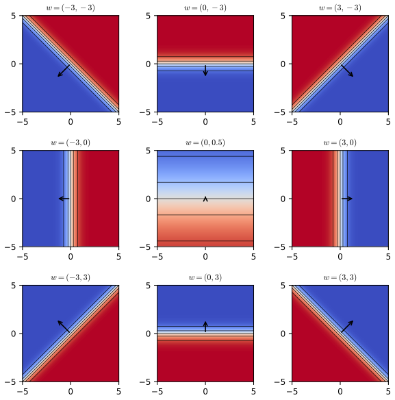
pp. 339–340 The rule \(f(\bm x)=\ind(\bm w^\T\bm x+b>0)\) (10.4, 10.5) is a linear classifier: it splits the input space into two half-spaces by the hyperplane with normal \(\bm w\) through the point \(\bm x_0\) with \(b=-\bm w^\T\bm x_0\) (Figure 10.1a, a sketch). If some hyperplane puts every training example on the correct side, the data are linearly separable; the two-feature iris data with Virginica against the rest are not (Figure 10.1b). The direction of \(\bm w\) sets the orientation of the boundary and its length \(\|\bm w\|\) the steepness of the sigmoid across it (Figure 10.2).
10.2.2 Nonlinear classifiers
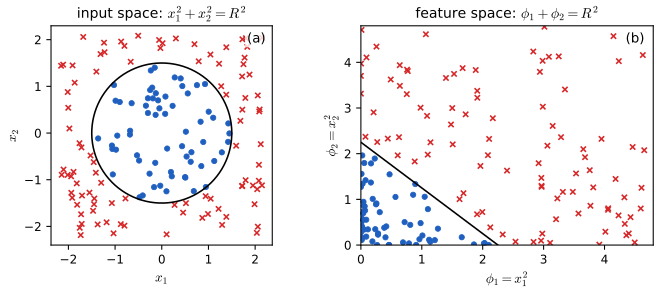
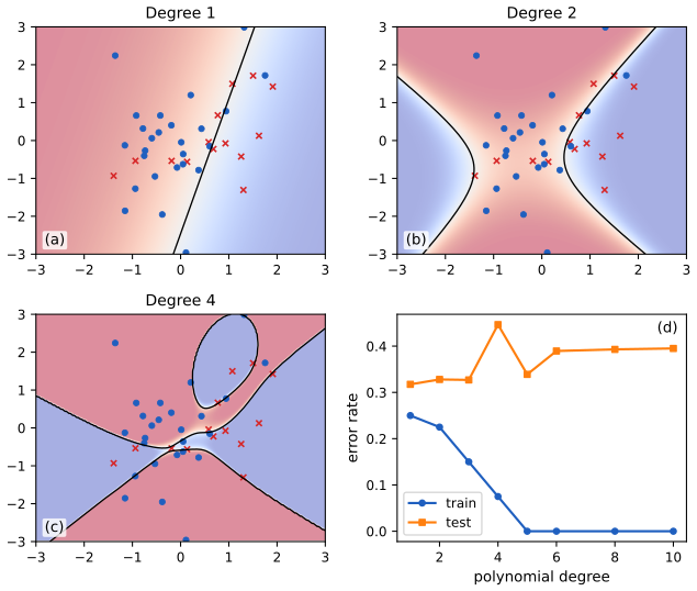
pp. 340–342 A problem that is not linearly separable in \(\bm x\) can become separable in transformed features \(\bm\phi(\bm x)\), and the model stays linear in the parameters, so all the machinery below applies unchanged with \(\bm x_n\) replaced by \(\bm\phi(\bm x_n)\). Example: \(\bm\phi(x_1,x_2)=[1,x_1^2,x_2^2]\) and \(\bm w=[-R^2,1,1]\) give \(\bm w^\T\bm\phi=x_1^2+x_2^2-R^2\), a circular boundary of radius \(R\) in the input plane and a straight line in the feature plane (Figure 10.3). Higher-degree polynomial features give more flexible boundaries and, as in Section 1.2.2.2, eventually overfit (Figure 10.4); weight decay (Section 10.2.7) is the remedy.
10.2.3 Maximum likelihood estimation
pp. 342–345 Objective (10.2.3.1). Absorb the bias into \(\bm w\). The mean negative log-likelihood is \[ \operatorname{NLL}(\bm w)=-\frac1N\sum_{n=1}^N\big[y_n\log\mu_n+(1-y_n)\log(1-\mu_n)\big]=\frac1N\sum_{n=1}^NH_{\rm ce}(y_n,\mu_n), \tag{10.8, 10.9} \] the average binary cross entropy \(H_{\rm ce}(p,q)=-[p\log q+(1-p)\log(1-q)]\) (10.10), equal to \(\frac1N\sum_n\log(1+e^{-\tilde y_na_n})\) (10.13). Optimisation (10.2.3.2). The MLE solves \(\nabla\operatorname{NLL}(\bm w)=\bm 0\) (10.14); any gradient method will do, provided the stationary point is a global minimiser, which needs convexity.
10.2.3.3 Deriving the gradient
pp. 343–344 With \(a_n=\bm w^\T\bm x_n\) and \(\mu_n=\sigma(a_n)\), the chain rule and \(\sigma'=\sigma(1-\sigma)\) give \(\partial_{w_d}\mu_n=\mu_n(1-\mu_n)x_{nd}\) (10.16), hence \(\nabla_{\bm w}\log\mu_n=(1-\mu_n)\bm x_n\) (10.17) and \(\nabla_{\bm w}\log(1-\mu_n)=-\mu_n\bm x_n\) (10.18). Combining, \[ \nabla_{\bm w}\operatorname{NLL}(\bm w)=\frac1N\sum_{n=1}^N(\mu_n-y_n)\bm x_n=\frac1N\bm X^\T(\bm\mu-\bm y). \tag{10.21, 10.22} \] The gradient averages the inputs weighted by the error signal \(e_n=\mu_n-y_n\in(-1,1)\): a correctly classified example far from the boundary contributes almost nothing.
10.2.3.4 Deriving the Hessian
pp. 344–345 Differentiating (10.21) once more, \(\partial\mu_n/\partial\bm w=\mu_n(1-\mu_n)\bm x_n\), so \[ \bm H(\bm w)=\nabla^2\operatorname{NLL}(\bm w)=\frac1N\sum_{n=1}^N\mu_n(1-\mu_n)\,\bm x_n\bm x_n^\T=\frac1N\bm X^\T\bm S\bm X,\quad\bm S=\diag(\mu_n(1-\mu_n)). \tag{10.23, 10.24} \] Since \(0<\mu_n(1-\mu_n)\le\frac14\), \(\bm H\) is positive semi-definite, so the NLL is convex, and it is strictly convex (a unique minimiser if one exists) exactly when \(\bm X\) has full column rank.
Filling the gap 10.3: gradient, Hessian, convexity, and the rank condition the book omits pp. 343–345, (10.21)–(10.25)
Derivation
Gradient. Write \(\ell_n(\bm w)=\log(1+e^{a_n})-y_na_n\) with \(a_n=\bm x_n^\T\bm w\); this is \(-[y_n\log\mu_n+(1-y_n)\log(1-\mu_n)]\) because \(\log\mu_n=a_n-\log(1+e^{a_n})\) and \(\log(1-\mu_n)=-\log(1+e^{a_n})\). Then \(\frac{\d\ell_n}{\d a_n}=\sigma(a_n)-y_n=\mu_n-y_n\), and \(\partial a_n/\partial\bm w=\bm x_n\), which gives (10.21) in one line, without the cancellation steps (10.19)–(10.20). The second derivative in \(a_n\) is \(\sigma'(a_n)=\mu_n(1-\mu_n)\), so \(\nabla^2\ell_n=\mu_n(1-\mu_n)\bm x_n\bm x_n^\T\) (10.23).
Convexity. For any \(\bm v\in\R^D\), \(\bm v^\T\bm H\bm v=\frac1N\sum_n\mu_n(1-\mu_n)(\bm x_n^\T\bm v)^2\ge0\). Writing \(\bm S^{1/2}\) for the diagonal square root, this is \(\frac1N\|\bm S^{1/2}\bm X\bm v\|_2^2\), the book's (10.25).
Strictness, a correction. The book concludes from (10.25) that \(\bm H\) is positive definite "since \(\mu_n>0\) for all \(n\)". That needs more: since every diagonal entry of \(\bm S\) is strictly positive, \(\bm S^{1/2}\bm X\bm v=\bm 0\iff\bm X\bm v=\bm 0\). So \(\bm v^\T\bm H\bm v=0\) for some \(\bm v\ne\bm 0\) exactly when the columns of \(\bm X\) are linearly dependent. Hence \(\bm H\) is positive definite for all \(\bm w\) iff \(\operatorname{rank}\bm X=D\) (this fails, for example, if two features are identical or if \(N<D\)); otherwise \(\operatorname{NLL}\) is convex but constant along the null directions of \(\bm X\), and the minimiser, if it exists, is a whole affine subspace. In numerical practice, strict positivity of \(\mu_n(1-\mu_n)\) is also lost to floating point when \(|a_n|\) exceeds about 36, which is where the "close to singular" remark of the book applies.
Numerical confirmation. On the iris petal measurements the smallest eigenvalue of \(\bm H\) at a random \(\bm w\) is about \(7.7\times10^{-3}\) (positive), while duplicating a column of \(\bm X\) makes the smallest eigenvalue zero to machine precision. \(\square\)
Filling the gap 10.2: Result 10.1 (existence and uniqueness of the MLE; separable data) pp. 344–345, p. 365 (the MLE "at infinity")
Statement. Let \(\tilde y_n\in\{\pm1\}\) and call a direction \(\bm v\) separating if \(\tilde y_n\bm x_n^\T\bm v\ge0\) for all \(n\), and strictly separating if \(>0\) for all \(n\). (a) If no nonzero \(\bm v\) is separating, then \(\operatorname{NLL}\) is coercive (\(\to\infty\) as \(\|\bm w\|\to\infty\)), so a minimiser exists; if moreover \(\operatorname{rank}\bm X=D\) it is unique. (b) If a strictly separating \(\bm v\) exists (the data are linearly separable), then \(\operatorname{NLL}(t\bm v)\downarrow0\) as \(t\to\infty\), the infimum 0 is not attained, and no MLE exists.
Proof
(b) With \(m_n=\tilde y_n\bm x_n^\T\bm v>0\), \(\operatorname{NLL}(t\bm v)=\frac1N\sum_n\log(1+e^{-tm_n})\), which is strictly decreasing in \(t\) and tends to 0; but \(\operatorname{NLL}(\bm w)>0\) for every finite \(\bm w\) because each term \(\log(1+e^{-\tilde y_na_n})\) is strictly positive. So the infimum is not attained.
(a) Let \(g(\bm w)=\frac1N\sum_n\log(1+e^{-\tilde y_n\bm x_n^\T\bm w})\). Suppose it is not coercive: there are \(\bm w_k\) with \(\|\bm w_k\|\to\infty\) and \(g(\bm w_k)\le M\). Pass to a subsequence with \(\bm w_k/\|\bm w_k\|\to\bm v\), \(\|\bm v\|=1\). Since \(\log(1+e^{-m})\ge\max(0,-m)\) for every \(m\), \(M\ge g(\bm w_k)\ge\frac1N\max_n\max(0,-\tilde y_n\bm x_n^\T\bm w_k)\), so \(\max(0,-\tilde y_n\bm x_n^\T\bm w_k/\|\bm w_k\|)\le NM/\|\bm w_k\|\to0\). In the limit \(-\tilde y_n\bm x_n^\T\bm v\le0\), i.e. \(\tilde y_n\bm x_n^\T\bm v\ge0\) for all \(n\): \(\bm v\) is a nonzero separating direction, a contradiction. So \(g\) is a continuous coercive function on \(\R^D\) and attains its minimum. Uniqueness follows from strict convexity (gap 10.3) when \(\operatorname{rank}\bm X=D\). (The case with a separating but not strictly separating direction is the "quasi-complete separation" of Albert and Anderson (1984); the MLE may or may not exist there.) \(\square\)
What to expect on separable data. Every optimiser run on separable data drives \(\|\bm w\|\to\infty\), slowly, like \(\log t\) for gradient descent, and the direction of \(\bm w\) approaches the maximum-margin separator (Soudry et al., 2018). Numerically: for the 22 separable points of Figure 10.13 the penalised solution has norms 1.05, 1.95, 3.05, 4.25 for penalties \(10^{-1},\dots,10^{-4}\) and its direction has cosine 0.9998 with the hard-margin SVM direction at the smallest penalty. A prior (Section 10.2.7) or early stopping is therefore not a luxury: it is what makes the problem well posed.
See also: Elements of Statistical Learning, Section 4.4.1 (fitting by Newton-Raphson); Bayesian and Probabilistic ML, logistic regression demo.
10.2.4 Stochastic gradient descent
pp. 345–346 With a minibatch of size one, the gradient step on the NLL is \[ \bm w_{t+1}=\bm w_t-\eta_t\nabla\operatorname{NLL}_n(\bm w_t)=\bm w_t-\eta_t(\mu_n-y_n)\bm x_n, \tag{10.28} \] where the example index \(n\) is drawn afresh at each step. The book states that, because the objective is convex, this converges to the global optimum if the step size is decayed appropriately. Two qualifications are made precise below: the rate needs strong convexity (a penalty or a full-rank bounded problem), and on separable data there is no optimum to converge to.
Filling the gap 10.4: a convergence rate for SGD on the penalised logistic loss p. 346, Section 8.4.3
Proof
Setting. Let \(F(\bm w)=\frac1N\sum_nf_n(\bm w)+\frac\mu2\|\bm w\|^2\) with \(f_n(\bm w)=\log(1+e^{\bm x_n^\T\bm w})-y_n\bm x_n^\T\bm w\), \(\mu>0\) (the penalty of Section 10.2.7 on all coordinates). Let \(R=\max_n\|\bm x_n\|\). \(F\) is \(\mu\)-strongly convex, so it has a unique minimiser \(\bm w^*\), and \(\frac\mu2\|\bm w^*\|^2\le F(\bm w^*)\le F(\bm 0)=\log2\), so \(\|\bm w^*\|\le\rho:=\sqrt{2\log2/\mu}\). Run projected SGD: \(\bm w_{t+1}=\Pi_\rho(\bm w_t-\eta_t\bm g_t)\), where \(\Pi_\rho\) projects onto the ball \(\{\|\bm w\|\le\rho\}\), \(\bm g_t=\nabla f_{n_t}(\bm w_t)+\mu\bm w_t\), and \(n_t\) is uniform and independent of the past. Since \(|\mu_n-y_n|\le1\), \(\|\bm g_t\|\le R+\mu\rho=:G\), and \(\E[\bm g_t\given\bm w_t]=\nabla F(\bm w_t)\).
Claim. With \(\eta_t=1/(\mu t)\), \(\E\|\bm w_t-\bm w^*\|^2\le\dfrac{2G^2}{\mu^2\,t}\) for all \(t\ge2\).
Proof. Projection onto a convex set containing \(\bm w^*\) does not increase the distance to \(\bm w^*\), so \(\|\bm w_{t+1}-\bm w^*\|^2\le\|\bm w_t-\bm w^*\|^2-2\eta_t\bm g_t^\T(\bm w_t-\bm w^*)+\eta_t^2G^2\). Take the conditional expectation. By \(\mu\)-strong convexity and \(\nabla F(\bm w^*)=\bm 0\), \(\nabla F(\bm w)^\T(\bm w-\bm w^*)\ge F(\bm w)-F(\bm w^*)+\frac\mu2\|\bm w-\bm w^*\|^2\ge\mu\|\bm w-\bm w^*\|^2\). With \(a_t=\E\|\bm w_t-\bm w^*\|^2\), \(a_{t+1}\le(1-2\mu\eta_t)a_t+\eta_t^2G^2=(1-\tfrac2t)a_t+\tfrac{G^2}{\mu^2t^2}\). At \(t=1\) the coefficient is \(-1\), so \(a_2\le G^2/\mu^2=c/2\) with \(c:=2G^2/\mu^2\). If \(a_t\le c/t\) for some \(t\ge2\), then \(a_{t+1}\le\frac ct-\frac{2c}{t^2}+\frac{c/2}{t^2}\le\frac ct-\frac c{t^2}=\frac{c(t-1)}{t^2}\le\frac c{t+1}\), because \((t-1)(t+1)\le t^2\). Induction gives the claim. \(\square\)
Remarks. (i) Without a penalty the loss is convex but not strongly convex, and the step sizes must satisfy the Robbins–Monro conditions \(\sum\eta_t=\infty\), \(\sum\eta_t^2<\infty\) for convergence (Robbins and Monro, 1951); the rate is then only \(O(1/\sqrt t)\) in the objective for the averaged iterate. (ii) On separable data there is no minimiser, and no choice of step schedule makes \(\bm w_t\) converge; \(\|\bm w_t\|\) grows without bound (Result 10.1). (iii) Numerically, with \(\mu=0.5\) on the standardised iris petal width and steps \(\eta_t=1/(\mu(t+10))\) (unprojected), the mean squared distance to \(\bm w^*\) over 40 runs is \(9.8\times10^{-4}\) after 500 steps and \(8\times10^{-5}\) after 4000, a fall by a factor of 12, at least the factor 8 that the \(1/t\) law predicts.
See also: Foundations of Deep Learning, Chapter 7 (gradient descent).
10.2.5 Perceptron algorithm
p. 346 The perceptron (Rosenblatt, 1958) is the deterministic classifier \(f(\bm x_n;\bm\theta)=\ind(\bm w^\T\bm x_n+b>0)\) (10.29): logistic regression with the sigmoid replaced by the Heaviside step. The step is not differentiable, so Rosenblatt used the error-correction rule \[ \bm w_{t+1}=\bm w_t-\eta_t(\hat y_n-y_n)\bm x_n \tag{10.30} \] on a randomly chosen example: nothing happens if the prediction \(\hat y_n\) is right; if \(y_n=1,\hat y_n=0\) then \(\bm w\leftarrow\bm w+\eta\bm x_n\), and if \(y_n=0,\hat y_n=1\) then \(\bm w\leftarrow\bm w-\eta\bm x_n\). Comparing with (10.28), it is SGD for logistic regression with the soft probability \(\mu_n\) replaced by the hard prediction \(\hat y_n\). The step size can be set to 1, since only the direction of \(\bm w\) matters for the boundary.
Filling the gap 10.5: the perceptron converges iff the data are separable (Novikoff's mistake bound) p. 346, [Nov62]
Proof
Use \(\tilde y_n\in\{\pm1\}\) and absorb the bias (\(\bm x_n\to(1,\bm x_n)\)). Starting from \(\bm w_0=\bm 0\), the rule (10.30) with \(\eta=1\) reads \(\bm w\leftarrow\bm w+\tilde y_n\bm x_n\) at a mistake, and a mistake implies \(\tilde y_n\bm w^\T\bm x_n\le0\) (for \(y_n=1\) the prediction is wrong iff \(\bm w^\T\bm x_n\le0\); for \(y_n=0\) iff \(\bm w^\T\bm x_n>0\)).
Theorem (Novikoff, 1962). Suppose \(\|\bm x_n\|\le R\) for all \(n\) and there is a unit vector \(\bm w^*\) with \(\tilde y_n\bm w^{*\T}\bm x_n\ge\gamma>0\) for all \(n\). Then the perceptron makes at most \((R/\gamma)^2\) mistakes, whatever the order in which examples are presented, and then stops changing.
Proof. Let \(\bm w_k\) be the weights after \(k\) mistakes, made on examples \(n_1,\dots,n_k\). Progress: \(\bm w^{*\T}\bm w_{k+1}=\bm w^{*\T}\bm w_k+\tilde y\bm w^{*\T}\bm x\ge\bm w^{*\T}\bm w_k+\gamma\), so \(\bm w^{*\T}\bm w_k\ge k\gamma\). Growth: \(\|\bm w_{k+1}\|^2=\|\bm w_k\|^2+2\tilde y\bm w_k^\T\bm x+\|\bm x\|^2\le\|\bm w_k\|^2+R^2\) because the middle term is \(\le0\) at a mistake, so \(\|\bm w_k\|^2\le kR^2\). By Cauchy–Schwarz, \(k\gamma\le\bm w^{*\T}\bm w_k\le\|\bm w_k\|\le\sqrt kR\), i.e. \(k\le(R/\gamma)^2\). \(\square\)
Converse. If the data are not separable, no \(\bm w\) classifies every example correctly, so after any finite number of updates some example is still misclassified and will eventually be drawn: the perceptron never stops. (Unlike logistic regression it also has no objective function that it is decreasing, so the weights cycle rather than settle.)
Numerical confirmation. On 80 well-separated points in the plane the perceptron makes 1 mistake against the bound \((R/\gamma)^2=5\) (\(\gamma\) from a hard-margin SVM); on the non-separable iris petal problem it is still making errors after 200 passes (2707 mistakes in total). \(\square\)
See also: Bayesian and Probabilistic ML, Section 4.1.7 (the perceptron algorithm).
10.2.6 Iteratively reweighted least squares
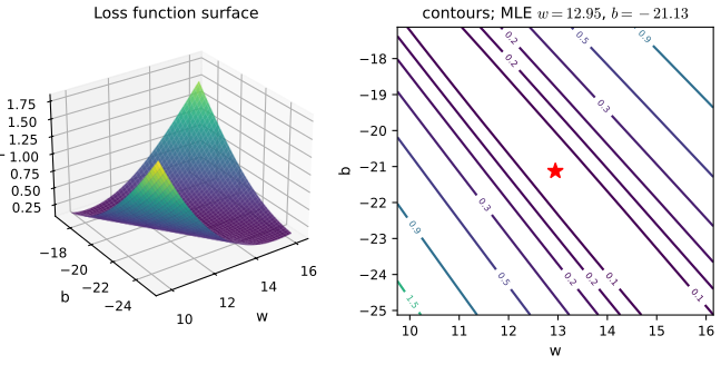
pp. 346–348 Gradient descent uses only first derivatives and is slow when the loss surface has steep and shallow directions at once, as in Figure 10.5. Newton's method uses the curvature. For logistic regression the Newton step \(\bm w_{t+1}=\bm w_t-\bm H_t^{-1}\bm g_t\) (10.31, 10.36), with \(\bm g=\frac1N\bm X^\T(\bm\mu-\bm y)\) and \(\bm H=\frac1N\bm X^\T\bm S\bm X\), can be rearranged as a weighted least-squares problem: \[ \bm w_{t+1}=(\bm X^\T\bm S_t\bm X)^{-1}\bm X^\T\bm S_t\bm z_t,\qquad z_{t,n}=\bm w_t^\T\bm x_n+\frac{y_n-\mu_{t,n}}{\mu_{t,n}(1-\mu_{t,n})}, \tag{10.40, 10.42} \] the minimiser of \(\sum_nS_{t,n}(z_{t,n}-\bm w_t^\T\bm x_n)^2\) (10.43); the weights \(S_{t,n}=\mu_{t,n}(1-\mu_{t,n})\) change at every iteration, hence iteratively reweighted least squares (Algorithm 10.1).
Algorithm 10.1: iteratively reweighted least squares (IRLS)
Start with \(\bm w=\bm 0\). Repeat until converged: for each \(n\), \(a_n=\bm w^\T\bm x_n\), \(\mu_n=\sigma(a_n)\), \(s_n=\mu_n(1-\mu_n)\), \(z_n=a_n+(y_n-\mu_n)/s_n\); then \(\bm S=\diag(s_{1:N})\) and \(\bm w=(\bm X^\T\bm S\bm X)^{-1}\bm X^\T\bm S\bm z\). (Python: irls_wls in code/ch10_logistic_regression.py; irls adds step halving, which keeps it monotone from any start.)
Filling the gap 10.6: from Newton to IRLS, and Fisher scoring is Newton here pp. 346–348, (10.36)–(10.43)
Derivation
Algebra. The factors \(\frac1N\) in \(\bm g\) and \(\bm H\) cancel in \(\bm H^{-1}\bm g\), so \(\bm w_{t+1}=\bm w_t+(\bm X^\T\bm S_t\bm X)^{-1}\bm X^\T(\bm y-\bm\mu_t)\) (10.37). Insert \(\bm w_t=(\bm X^\T\bm S_t\bm X)^{-1}(\bm X^\T\bm S_t\bm X)\bm w_t\) and factor: \(\bm w_{t+1}=(\bm X^\T\bm S_t\bm X)^{-1}\bm X^\T[\bm S_t\bm X\bm w_t+\bm y-\bm\mu_t]\) (10.39). Since \(\bm S_t\) is diagonal and invertible, \(\bm S_t\bm X\bm w_t+\bm y-\bm\mu_t=\bm S_t[\bm X\bm w_t+\bm S_t^{-1}(\bm y-\bm\mu_t)]=\bm S_t\bm z_t\) (10.40, 10.41).
Weighted least squares. The objective \(\sum_nS_n(z_n-\bm w^\T\bm x_n)^2=(\bm z-\bm X\bm w)^\T\bm S(\bm z-\bm X\bm w)\) has gradient \(-2\bm X^\T\bm S(\bm z-\bm X\bm w)\); setting it to zero gives the weighted normal equations \(\bm X^\T\bm S\bm X\bm w=\bm X^\T\bm S\bm z\), whose solution is (10.40). Interpretation: near the current iterate, \(\mu_n\approx\mu_{t,n}+s_{t,n}(a_n-a_{t,n})\), so the working response \(z_n\) is the value of the logit that would make the linearised mean equal \(y_n\), and \(s_n\) is the inverse variance of that pseudo-observation. This is why a logistic regression can be fitted with a weighted linear-regression routine.
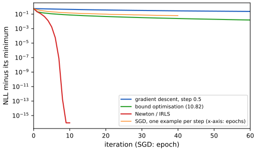
Convergence. Newton's method converges quadratically near a nondegenerate minimiser because the Hessian is Lipschitz: with \(s(a)=\sigma(a)(1-\sigma(a))\) one has \(s'=\sigma(1-\sigma)(1-2\sigma)\), \(|s'|\le\frac1{6\sqrt3}\), so \(\|\bm H(\bm w)-\bm H(\bm w')\|\le\frac{R^3}{6\sqrt3}\|\bm w-\bm w'\|\) with \(R=\max_n\|\bm x_n\|\). But a full step from a bad start can increase the loss (the Hessian is tiny where the sigmoid saturates, so the step is huge); step halving until the loss decreases restores global convergence. On the iris petal-width problem of Figure 10.5, starting at \(\bm w=\bm 0\), the gap \(\operatorname{NLL}(\bm w_t)-\min\operatorname{NLL}\) is \(0.58,0.21,0.11,4.6\times10^{-2},1.3\times10^{-2},1.7\times10^{-3},5.6\times10^{-5},8.0\times10^{-8}\) after \(0,\dots,7\) iterations: the error is raised to a power above 1 at each step (Figure 10.S2).
Fisher scoring. The book says Fisher scoring replaces the Hessian by its expectation, the Fisher information, "which is independent of the data and can be precomputed". For logistic regression this is not the case, and in fact nothing changes: \(\bm H=\frac1N\bm X^\T\bm S\bm X\) depends on the parameters and on the inputs but not on the labels, so \(\E_{\bm y}[\bm H]=\bm H\); Fisher scoring, Newton's method and IRLS are the same algorithm. This is the general fact that for a generalised linear model with the canonical link the observed and expected information coincide (see Bayesian and Probabilistic ML, Section 4.3.6). The Fisher information \(\bm F(\bm w)=\bm X^\T\bm S(\bm w)\bm X\) changes with \(\bm w\), so it cannot be precomputed once either; for a non-canonical link such as the probit, the Hessian does depend on \(\bm y\) and the two methods differ. The check confirms that the logistic Hessian is identical for two different label vectors at the same \(\bm w\), and that it differs between \(\bm w=\bm 0\) and another \(\bm w\). \(\square\)
See also: Bayesian and Probabilistic ML, Section 4.3.3 (IRLS); the IRLS demo of Elements of Statistical Learning.
10.2.7 MAP estimation
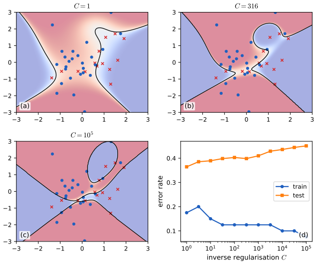
pp. 348–349 Maximum likelihood can overfit: to bend the boundary around the training points it needs large weights (the book quotes \(\|\hat{\bm w}\|\) growing from about 0.5 at degree 1 to about 60 at degree 4 in its Figure 10.4). Weight decay puts a zero-mean Gaussian prior on the weights, \(p(\bm w)=\N(\bm w\given\bm 0,C\bm I)\), and replaces the MLE by the MAP estimate, which minimises \[ \mathcal L(\bm w)=\operatorname{NLL}(\bm w)+\lambda\|\bm w\|_2^2,\qquad\lambda=1/C, \tag{10.47} \] with gradient and Hessian \(\nabla\mathcal L=\bm g(\bm w)+2\lambda\bm w\) and \(\nabla^2\mathcal L=\bm H(\bm w)+2\lambda\bm I\) (10.48–10.50): every optimiser above works unchanged after this small modification. Larger \(\lambda\) means a smaller prior variance and a less flexible model (Figure 10.6).
Filling the gap 10.7: the prior-to-penalty dictionary, existence, and the scale of \(\lambda\) pp. 348–349, (10.47)–(10.50)
Derivation
MAP is a penalised fit. Let \(\operatorname{NLL}_\Sigma(\bm w)=-\log p(\mathcal D\given\bm w)=N\cdot\operatorname{NLL}(\bm w)\) be the NLL summed over the data. Then \(-\log p(\bm w\given\mathcal D)=\operatorname{NLL}_\Sigma(\bm w)+\frac1{2C}\|\bm w\|^2+\mathrm{const}\), and dividing by \(N\) gives \(\operatorname{NLL}(\bm w)+\frac1{2CN}\|\bm w\|^2\). So (10.47) holds with \(\lambda=\frac1{2CN}\) for the averaged NLL (or, equivalently, with penalty \(\frac1{2C}\|\bm w\|^2\) on the summed NLL, which is the convention of most software, where \(C\) is the "inverse regularisation strength"). The book's "\(\lambda=1/C\)" is correct only up to this constant factor, which matters when comparing numbers with a library. Numerically, the minimiser of the mean NLL plus \(\frac1{2CN}\|\bm w\|^2\) (bias unpenalised) coincides with the fit of scikit-learn's LogisticRegression(C=C).
Existence and uniqueness. \(\mathcal L=\operatorname{NLL}+\lambda\|\bm w\|^2\) is the sum of a convex function and a strongly convex one with Hessian \(\succeq2\lambda\bm I\), so it is strongly convex (Hessian \(\bm H+2\lambda\bm I\succ0\) always, with no condition on \(\bm X\)); and it is coercive since \(\operatorname{NLL}\ge0\). A continuous coercive strongly convex function has exactly one minimiser, for separable and non-separable data alike. This is why the MAP estimate exists in Figure 10.13 when the MLE does not (Result 10.1).
The bias. The prior should usually not be put on the bias \(b\): shifting all logits by a constant is a genuine change of the class balance, not a sign of overfitting. In the code the first coordinate of \(\bm w\) is left unpenalised (the penalty matrix is \(\diag(0,1,\dots,1)\)), as in common software. With that choice the Hessian is \(\bm H+\lambda\diag(0,1,\dots,1)\) (positive definite when \(\bm X\) has full rank).
Effect on the size of the weights. In the simulated problem of Figure 10.4 the norm of the fitted weight vector for degree 4 is \(\|\hat{\bm w}\|=215\) (\(C=10^6\)), 173 (\(C=10^5\)), 25 (\(C=316\)) and 2.2 (\(C=1\)). \(\square\)
10.2.8 Standardization
p. 350 An isotropic prior \(\N(\bm 0,\lambda^{-1}\bm I)\) treats all weights alike, which presumes the features are on comparable scales. Standardising each feature, \(x_{nd}\mapsto(x_{nd}-\hat\mu_d)/\hat\sigma_d\) with the training-set mean and standard deviation (10.51–10.53), or rescaling to \([0,1]\) (min-max scaling), makes that assumption reasonable and also helps the optimiser.
Filling the gap 10.8: why scaling matters for MAP but not for the MLE, and for gradient descent p. 350
Derivation
MLE equivariance. Let \(\bm x'=\bm A\bm x+\bm c\) with \(\bm A\) invertible (this includes standardisation). A model with weights \(\bm w'\) and bias \(b'\) on \(\bm x'\) gives the logit \(\bm w'^\T\bm A\bm x+\bm w'^\T\bm c+b'\), which is the logit of the original model with \(\bm w=\bm A^\T\bm w'\) and \(b=b'+\bm w'^\T\bm c\). This is a bijection of parameters preserving every likelihood value, so the maximum-likelihood boundary and fitted probabilities are the same whichever scaling is used. Numerically: rescaling the iris petal width to \(3x+1\) multiplies the MLE slope by 1/3 and shifts the bias by exactly the predicted amount.
MAP is not equivariant. In the primed parametrisation \(\bm w'=\bm A^{-\T}\bm w\), so a penalty \(\lambda\|\bm w'\|^2\) equals \(\lambda\,\bm w^\T(\bm A^\T\bm A)^{-1}\bm w\) in the original parametrisation: it is the same as the isotropic penalty on \(\bm w\) only if \(\bm A\) is orthogonal. For a diagonal rescaling \(x'_d=s_dx_d\) the penalty is \(\lambda\sum_dw_d^2/s_d^2\): a feature with large numerical values (small units) needs only a small weight and is barely penalised, a feature with small numerical values needs a large weight and is penalised heavily. Standardising before fitting makes the penalty act on "effect per standard deviation", comparable across features. (Check: the penalised slope on \(3x+1\), times 3, differs from the penalised slope on \(x\).) The mean and standard deviation should be computed on the training set only and then applied unchanged to validation and test data.
Conditioning for first-order methods. Gradient descent with a fixed step \(\eta\) converges iff \(\eta<2/L\), \(L=\lambda_{\max}(\bm H)\), at a rate set by the condition number \(\lambda_{\max}/\lambda_{\min}\) of \(\bm H\). \(\bm H\) is a weighted version of the second-moment matrix of \((1,x)\), \(\begin{pmatrix}1&m\\m&m^2+s^2\end{pmatrix}\), with \(m\) the mean and \(s\) the standard deviation of the feature; this matrix is nearly singular (a long narrow valley) when \(|m|\gg s\) and is the identity when \(m=0,s=1\). For the iris petal width (\(m=1.20\), \(s=0.76\)) its condition number is about 14; after standardising it is 1. The demonstration shows the effect: the same loss in standardised coordinates has round contours (preset 3). \(\square\)
10.3 Multinomial logistic regression
pp. 350–351 For \(C>2\) classes the model replaces the sigmoid by the softmax of a vector of \(C\) logits: \[ p(y\given\bm x,\bm\theta)=\operatorname{Cat}\big(y\given\softmax(\bm W\bm x+\bm b)\big),\qquad p(y=c\given\bm x,\bm\theta)=\frac{e^{a_c}}{\sum_{c'=1}^Ce^{a_{c'}}}, \tag{10.54, 10.55} \] with \(\bm a=\bm W\bm x\) the vector of logits (bias absorbed into \(\bm W\)). Because the probabilities sum to one, one class can be "clamped", \(\bm w_C=\bm 0\), leaving \((C-1)\) weight vectors (for \(C=2\) a single one, recovering the binary model); the clamped form is \[ p(y=c\given\bm x,\bm W)=\frac{e^{\bm w_c^\T\bm x}}{1+\sum_{k=1}^{C-1}e^{\bm w_k^\T\bm x}}\quad(c<C). \tag{10.85} \] The classes are mutually exclusive. For multi-label problems (several tags per item) one instead fits \(C\) independent binary models, \(p(\bm y\given\bm x)=\prod_c\operatorname{Ber}(y_c\given\sigma(\bm w_c^\T\bm x))\) (10.56).
10.3.1 Linear and nonlinear classifiers
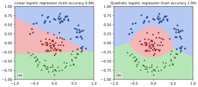
p. 351 The decision regions of the softmax classifier are convex polyhedra: \(\hat y=\argmax_ca_c\), and class \(c\) wins where \((\bm w_c-\bm w_k)^\T\bm x>0\) for all \(k\ne c\), an intersection of half-spaces (Figure 10.7a). Feature maps give nonlinear boundaries: with \(\bm\phi(\bm x)=[1,x_1,x_2,x_1^2,x_2^2,x_1x_2]\) (10.57) the boundaries are conics (Figure 10.7b).
10.3.2 Maximum likelihood estimation
pp. 351–353 With one-hot labels \(y_{nc}=\ind(y_n=c)\) and \(\mu_{nc}=\softmax(\bm a_n)_c\), the mean NLL is the average multiclass cross entropy, \[ \operatorname{NLL}(\bm W)=-\frac1N\sum_{n}\sum_{c}y_{nc}\log\mu_{nc}=\frac1N\sum_nH_{\rm ce}(\bm y_n,\bm\mu_n),\quad H_{\rm ce}(\bm p,\bm q)=-\sum_cp_c\log q_c. \tag{10.58, 10.59} \] The softmax Jacobian is \(\partial\mu_c/\partial a_j=\mu_c(\delta_{cj}-\mu_j)\) (10.60), i.e. \(\operatorname{diag}(\bm\mu)-\bm\mu\bm\mu^\T\) in matrix form, and the gradient is again "error times input", \[ \nabla_{\bm w_j}\operatorname{NLL}=\frac1N\sum_n(\mu_{nj}-y_{nj})\bm x_n,\qquad \bm g(\bm W)=\frac1N\sum_n\bm x_n(\bm\mu_n-\bm y_n)^\T, \tag{10.67, 10.68} \] with Hessian \[ \bm H(\bm w)=\frac1N\sum_n\big(\diag(\bm\mu_n)-\bm\mu_n\bm\mu_n^\T\big)\otimes(\bm x_n\bm x_n^\T),\qquad \bm H_{c,c'}=\frac1N\sum_n\mu_{nc}(\delta_{cc'}-\mu_{nc'})\bm x_n\bm x_n^\T, \tag{10.69, 10.70} \] \(\otimes\) the Kronecker product, for the weights stacked class by class.
Filling the gap 10.9: Exercise 10.1, the softmax Jacobian, gradient and Hessian, and why the full Hessian is only semi-definite pp. 352–353, Exercise 10.1
Derivation
Jacobian (10.60, 10.119). \(\mu_c=e^{a_c}/Z\), \(Z=\sum_ke^{a_k}\), and \(\partial Z/\partial a_j=e^{a_j}\). By the quotient rule, \(\frac{\partial\mu_c}{\partial a_j}=\frac{\delta_{cj}e^{a_c}Z-e^{a_c}e^{a_j}}{Z^2}=\mu_c\delta_{cj}-\mu_c\mu_j=\mu_c(\delta_{cj}-\mu_j)\).
Gradient (10.67, 10.120). The book's chain-rule calculation (10.63)–(10.67) works; there is a shorter route. Since \(\sum_cy_{nc}=1\), \(-\sum_cy_{nc}\log\mu_{nc}=-\sum_cy_{nc}(a_{nc}-\lse(\bm a_n))=\lse(\bm a_n)-\sum_cy_{nc}a_{nc}\), where \(\lse(\bm a)=\log\sum_ke^{a_k}\) has \(\partial\lse/\partial a_j=\mu_j\). So \(\partial\ell_n/\partial a_{nj}=\mu_{nj}-y_{nj}\), and since \(a_{nj}=\bm w_j^\T\bm x_n\), \(\nabla_{\bm w_j}\ell_n=(\mu_{nj}-y_{nj})\bm x_n\). The same \(\lse\) form is what software evaluates, avoiding \(\log\) of an underflowed probability (10.73).
Hessian (10.69, 10.121). From the previous step, \(\partial^2\ell_n/\partial a_{nj}\partial a_{nk}=\mu_{nj}(\delta_{jk}-\mu_{nk})\), and \(\partial a_{nj}/\partial\bm w_j=\bm x_n\), so the \((j,k)\) block of the Hessian of \(\ell_n\) is \(\mu_{nj}(\delta_{jk}-\mu_{nk})\bm x_n\bm x_n^\T\); stacking gives (10.69). (The book's (10.121) has an overall minus sign because it differentiates the log-likelihood.)
Positive semi-definiteness, and what the book misses. Let \(\bm v=(\bm u_1,\dots,\bm u_C)\) be a stacked vector with blocks \(\bm u_c\in\R^D\), and put \(r_{nc}=\bm u_c^\T\bm x_n\). Then \[ \bm v^\T\bm H\bm v=\frac1N\sum_n\Big[\sum_c\mu_{nc}r_{nc}^2-\Big(\sum_c\mu_{nc}r_{nc}\Big)^2\Big]=\frac1N\sum_n\operatorname{var}_{c\sim\bm\mu_n}[r_{nc}]\ \ge0, \] the variance of \(r_{nc}\) when \(c\) is drawn from \(\bm\mu_n\). So \(\bm H\succeq0\) and the NLL is convex. Because every \(\mu_{nc}>0\), the variance vanishes iff \(r_{nc}\) is the same for all \(c\): \(\bm u_c^\T\bm x_n=\bm u_1^\T\bm x_n\) for all \(c,n\). One family of solutions is \(\bm u_1=\dots=\bm u_C=\bm u\) (any \(\bm u\)): adding the same vector to every class's weights leaves all probabilities unchanged. If \(\operatorname{rank}\bm X=D\), these are the only solutions (then \(\bm u_c-\bm u_1\) is orthogonal to every \(\bm x_n\), hence zero). So the full \(CD\times CD\) Hessian has a null space of dimension exactly \(D\): it is positive semi-definite but not positive definite, contrary to the last sentence of Exercise 10.1c as stated; in the book's own words the parameters are "unidentifiable" without clamping (Section 10.3.5). Numerically, for 3 classes and 3 features the 9×9 Hessian has exactly 3 zero eigenvalues, with null vectors \(\bm 1\otimes\bm e_j\).
Clamping restores definiteness. Restrict to \(\bm u_C=\bm 0\). Then the variance is zero iff all \(r_{nc}=r_{nC}=0\), i.e. \(\bm u_c\perp\bm x_n\) for all \(n\), so \(\bm u_c=\bm 0\) when \(\operatorname{rank}\bm X=D\): the \((C-1)D\times(C-1)D\) Hessian of the clamped model (10.85) is positive definite, and the NLL is strictly convex with a unique minimiser when the data are not separable (the multiclass analogue of Result 10.1). \(\square\)
See also: Bayesian and Probabilistic ML, Section 4.3.4 (multiclass logistic regression); Introduction to Statistical Learning, Section 4.3.5.
10.3.3 Gradient-based optimization
p. 354 The gradient (10.68) gives SGD directly, and the Hessian (10.69) gives a Newton method, but the latter costs \(O((CD)^3)\) per step; quasi-Newton methods such as L-BFGS (Section 8.3.2) are therefore the usual choice for a moderate number of features, and the bound-optimisation iteration below is another (the code uses L-BFGS). All of them need \(\log p(y=c\given\bm x)=a_c-\lse(\bm a)\) (10.73), computed with the log-sum-exp trick: \(\lse(\bm a)=m+\log\sum_ke^{a_k-m}\) for \(m=\max_ka_k\), which is exact in real arithmetic for every \(m\) and avoids overflow; libraries therefore expose a cross-entropy that takes the logits, not the probabilities.
10.3.4 Bound optimization
pp. 354–355 A bound-optimisation (or majorise–minimise, MM) algorithm repeatedly minimises a simple function that lies above the objective and touches it at the current point (Section 8.7). If \(\nabla^2\operatorname{NLL}_\Sigma\preceq\bm B\) for a fixed matrix \(\bm B\) at all \(\bm w\), then for the summed NLL \[ \operatorname{NLL}_\Sigma(\bm w)\le\operatorname{NLL}_\Sigma(\bm w_t)+(\bm w-\bm w_t)^\T\bm g_t+\tfrac12(\bm w-\bm w_t)^\T\bm B(\bm w-\bm w_t), \tag{10.74} \] and minimising the right-hand side gives the update \(\bm w_{t+1}=\bm w_t-\bm B^{-1}\bm g_t\) (10.75, 10.81): Newton's update with a constant curvature matrix, which can be inverted once. For multinomial logistic regression, Böhning's matrix \[ \bm H(\bm w)\preceq\bm B:=\tfrac12\big[\bm I-\bm 1\bm 1^\T/C\big]\otimes\Big(\sum_n\bm x_n\bm x_n^\T\Big) \tag{10.79} \] works, and in the binary case \(\bm B=\frac14\bm X^\T\bm X\), because \(\mu(1-\mu)\le\frac14\) (10.80). The binary update is \[ \bm w_{t+1}=\bm w_t-4(\bm X^\T\bm X)^{-1}\bm X^\T(\bm\mu_t-\bm y)=\bm w_t+4(\bm X^\T\bm X)^{-1}\bm X^\T(\bm y-\bm\mu_t); \tag{10.82} \] compare Newton (10.83), which uses \((\bm X^\T\bm S_t\bm X)^{-1}\) in place of \(4(\bm X^\T\bm X)^{-1}\) and needs a new factorisation each iteration. The signs are written above for the NLL; the book writes (10.82) with a minus sign in front of \(\bm g_t=\bm X^\T(\bm y-\bm\mu_t)\), the gradient of the log-likelihood, which would move uphill on the NLL (see the notes on the book).
Filling the gap 10.10: the Böhning bound and monotonicity of the bound-optimisation iteration pp. 354–355, (10.74)–(10.82), [Boh92]
Proof
The bound. For one example, the Hessian block is \(\bm P=\diag(\bm\mu)-\bm\mu\bm\mu^\T\) (times \(\bm x\bm x^\T\)). For any \(\bm u\in\R^C\), \(\bm u^\T\bm P\bm u=\operatorname{var}_{c\sim\bm\mu}[u_c]\). By Popoviciu's inequality the variance of a variable taking values in \([\min u,\max u]\) is at most \(\frac14(\max_cu_c-\min_cu_c)^2\). For any two entries, \((u_i-u_j)^2\le2[(u_i-\bar u)^2+(u_j-\bar u)^2]\le2\sum_c(u_c-\bar u)^2\) with \(\bar u\) the mean, so \(\operatorname{var}_{\bm\mu}[\bm u]\le\frac12\sum_c(u_c-\bar u)^2=\frac12\bm u^\T(\bm I-\bm 1\bm 1^\T/C)\bm u\). Hence \(\bm P\preceq\frac12(\bm I-\bm 1\bm 1^\T/C)\) for every \(\bm\mu\) (the book's \(\succ\) in (10.79) should be \(\succeq\), since equality is attained). If \(\bm A\preceq\bm A'\) and \(\bm M\succeq0\) then \(\bm A\otimes\bm M\preceq\bm A'\otimes\bm M\) (the difference is \((\bm A'-\bm A)\otimes\bm M\), a Kronecker product of two positive semi-definite matrices, hence positive semi-definite). Summing over \(n\) with \(\bm M=\bm x_n\bm x_n^\T\) gives (10.79). For \(C=2\) the matrix \(\frac12(\bm I-\bm 1\bm 1^\T/2)\) restricted to the one free class is \(\frac14\), giving \(\frac14\bm X^\T\bm X\) (10.80).
The matrix is singular unless a class is clamped. \(\bm I-\bm 1\bm 1^\T/C\) annihilates \(\bm 1\), so \(\bm B\) is singular, mirroring the singular Hessian of gap 10.9. After clamping class \(C\), keep the leading \((C-1)\times(C-1)\) block: \(\bm I-\bm 1\bm 1^\T/C\) has this block with eigenvalues \(1\) (multiplicity \(C-2\)) and \(1/C\), so it is positive definite, and \(\bm B\) is invertible whenever \(\bm X^\T\bm X\succ0\). This is the matrix used in the code.
Monotonicity. Suppose \(\nabla^2\operatorname{NLL}_\Sigma(\bm\xi)\preceq\bm B\) for all \(\bm\xi\). Taylor's theorem with integral remainder gives \(\operatorname{NLL}_\Sigma(\bm w)=\operatorname{NLL}_\Sigma(\bm w_t)+\bm g_t^\T\bm\Delta+\int_0^1(1-s)\bm\Delta^\T\nabla^2\operatorname{NLL}_\Sigma(\bm w_t+s\bm\Delta)\bm\Delta\,\d s\le\operatorname{NLL}_\Sigma(\bm w_t)+\bm g_t^\T\bm\Delta+\frac12\bm\Delta^\T\bm B\bm\Delta=:Q(\bm w\given\bm w_t)\), \(\bm\Delta=\bm w-\bm w_t\): this is (10.74) (the book states it for the concave log-likelihood). \(Q\) is a strictly convex quadratic with minimiser \(\bm w_t-\bm B^{-1}\bm g_t\). So \(\operatorname{NLL}_\Sigma(\bm w_{t+1})\le Q(\bm w_{t+1}\given\bm w_t)\le Q(\bm w_t\given\bm w_t)=\operatorname{NLL}_\Sigma(\bm w_t)\): the loss never increases, with no step size to tune. Since \(\bm B\succeq\bm H(\bm w)\) the steps are never longer than Newton's and are conservative where the sigmoid saturates (\(\mu(1-\mu)\ll\frac14\)); where \(\mu\approx\frac12\) the two coincide: in the binary case at \(\bm w=\bm 0\) all \(\mu_n(1-\mu_n)=\frac14\), so the first bound step and the first Newton step are the same (confirmed numerically). The price is a linear rate (Figure 10.S2 and the demo), which the fixed \(\bm B\) cannot improve. \(\square\)
10.3.5 MAP estimation
pp. 355–356 The benefits of \(\ell_2\) regularisation (Section 10.2.7) carry over, with one more: without clamping, the model is not identifiable, since \(\bm w_c\mapsto\bm w_c+\bm u\) for all \(c\) changes nothing. With the penalty \[ \operatorname{PNLL}(\bm W)=-\sum_n\log p(y_n\given\bm x_n,\bm W)+\lambda\sum_c\|\bm w_c\|^2 \tag{10.86} \] the optimum automatically satisfies \(\sum_c\hat w_{cj}=0\) for every feature \(j\) (10.89), which selects one representative.
Filling the gap 10.11: the sum-to-zero property and the identifiability argument pp. 355–356, (10.86)–(10.89)
Derivation
Use the convention \(\operatorname{PNLL}(\bm W)=\operatorname{NLL}_\Sigma(\bm W)+\frac\lambda2\sum_c\|\bm w_c\|^2\) (the book's \(\lambda\|\cdot\|^2\) differs by a factor 2 in \(\lambda\), which only rescales the constant below). At a stationary point, by (10.67), \(-\sum_n(y_{nc}-\mu_{nc})\bm x_n+\lambda\bm w_c=\bm 0\) for each \(c\). Sum over \(c\): \(\lambda\sum_c\bm w_c=\sum_n\big(\sum_cy_{nc}-\sum_c\mu_{nc}\big)\bm x_n=\sum_n(1-1)\bm x_n=\bm 0\) (10.89), so for \(\lambda>0\), \(\sum_c\hat{\bm w}_c=\bm 0\).
Why this identifies the solution. The likelihood is invariant under \(\bm w_c\mapsto\bm w_c+\bm u\) for all \(c\); within this family the penalty \(\frac\lambda2\sum_c\|\bm w_c+\bm u\|^2\) is a strictly convex quadratic in \(\bm u\), minimised at \(\bm u=-\frac1C\sum_c\bm w_c\), i.e. at the representative with \(\sum_c\bm w_c=\bm 0\). So the penalised minimiser is the minimum-norm point of the family. Uniqueness of the minimiser itself follows because the Hessian of PNLL is \(\bm H+\lambda\bm I\succ0\) (\(\bm H\succeq0\) by gap 10.9), so PNLL is strictly convex.
A caveat. If the bias is left out of the penalty (as software usually does), the biases \(b_c\) are still unidentified: adding the same constant to all of them changes neither the likelihood nor the penalty, and the optimiser returns whatever representative its initialisation selects. In that case the sum-to-zero property holds for the penalised weights only; fix the bias by clamping one class or by centring after fitting. Numerically, with a penalty on all weights the sums over classes are zero to machine precision (\(10^{-15}\)). \(\square\)
10.3.6 Maximum entropy classifiers
pp. 356–357 Letting the features depend on the candidate class, \(\bm\phi(\bm x,c)\), gives the maximum-entropy (maxent) classifier \[ p(y=c\given\bm x,\bm w)=\frac{\exp(\bm w^\T\bm\phi(\bm x,c))}{Z(\bm w,\bm x)},\qquad Z(\bm w,\bm x)=\sum_{c'}\exp(\bm w^\T\bm\phi(\bm x,c')), \tag{10.90, 10.91} \] widely used in natural-language processing, where features such as "the label is person and the word follows Mr." tie a feature to a label. Multinomial logistic regression is the special case \(\bm\phi(\bm x,c)=[\bm 0,\dots,\bm x,\dots,\bm 0]\) with \(\bm x\) in block \(c\) (10.92), so that \(\bm w^\T\bm\phi=\bm w_c^\T\bm x\).
Filling the gap 10.12: why "maximum entropy"; the MLE matches the feature expectations pp. 356–357, Section 3.4.4
Proof
Special case. With the block features, \(\exp(\bm w^\T\bm\phi(\bm x,c))=\exp(\bm w_c^\T\bm x)\), and the normaliser is \(\sum_{c'}\exp(\bm w_{c'}^\T\bm x)\): exactly (10.54).
Maximum-likelihood fits match the empirical feature averages. The log-likelihood is \(\ell(\bm w)=\sum_n[\bm w^\T\bm\phi(\bm x_n,y_n)-\log Z(\bm w,\bm x_n)]\) and \(\nabla\ell=\sum_n[\bm\phi(\bm x_n,y_n)-\E_{p(c\given\bm x_n,\bm w)}\bm\phi(\bm x_n,c)]\). At the MLE, \(\sum_n\E_{p}[\bm\phi(\bm x_n,c)]=\sum_n\bm\phi(\bm x_n,y_n)\): the model's expected features equal the observed ones.
Maximum entropy. Let \(\mathcal Q\) be the set of conditional distributions \(q(c\given\bm x_n)\) (for the observed inputs) satisfying the same constraints, \(\sum_n\E_{q_n}\bm\phi(\bm x_n,c)=\sum_n\bm\phi(\bm x_n,y_n)\). For \(q\in\mathcal Q\) and \(p=p(\cdot\given\bm x_n,\bm w_{\rm MLE})\), using \(\log p_{nc}=\bm w^\T\bm\phi(\bm x_n,c)-\log Z_n\), \[ \sum_nH(q_n)=-\sum_n\sum_cq_{nc}\log p_{nc}-\sum_n\KL(q_n\|p_n)=-\bm w^\T\sum_n\bm\phi(\bm x_n,y_n)+\sum_n\log Z_n-\sum_n\KL(q_n\|p_n), \] since the middle term depends on \(q\) only through the constrained expectations. The same identity with \(q=p\) (which lies in \(\mathcal Q\)) shows \(\sum_nH(q_n)=\sum_nH(p_n)-\sum_n\KL(q_n\|p_n)\le\sum_nH(p_n)\), with equality iff \(q=p\). Hence the maxent classifier is the member of \(\mathcal Q\) of largest conditional entropy: it commits to nothing beyond what the feature constraints demand. \(\square\)
10.3.7 Hierarchical classification
pp. 357–358 When the labels form a taxonomy (animal, then dog or cat, then breed), the classifier should "hedge its bets" and predict the most precise label it is confident about. The book describes a simple recipe: give the model one binary output per node, use label smearing so that a training label is propagated to all its ancestors (a "golden retriever" image is also a "dog" and a "mammal"), and add a mutual-exclusion constraint among siblings (Figure 10.8, a sketch). Concretely, in a flat model the three probabilities \(p(\text{retriever}),p(\text{cat}),p(\text{bird})\) could all be near 1; with the constraint, \(p(\text{mammal}\given\bm x)+p(\text{bird}\given\bm x)=1\) and \(p(\text{dog}\given\bm x)+p(\text{cat}\given\bm x)=p(\text{mammal}\given\bm x)\). Implementation: at each internal node, a softmax over the node's children multiplies the parent's probability (see gap 10.13).
10.3.8 Handling large numbers of classes
pp. 358–359 Hierarchical softmax (10.3.8.1). A flat softmax needs the normaliser \(\sum_ce^{a_c}\), which costs \(O(C)\) per example and dominates when \(C\) is the vocabulary of a language. Arrange the classes at the leaves of a binary tree and give each internal node a logistic regression; the probability of a leaf is the product of the branch probabilities along the root-to-leaf path, so it costs \(O(\log C)\) in a balanced tree, e.g. \(p(y=\text{I'm}\given C)=0.57\times0.68\times0.72=0.28\) (10.96, Figure 10.9, a diagram). Putting frequent labels near the root (a Huffman tree) reduces the average path length further.
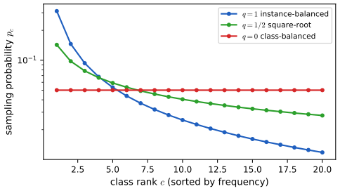
Class imbalance and the long tail (10.3.8.2). When the class counts \(N_c\) are very unequal, rare classes contribute little to the loss. Remedies: set the biases so that \(\softmax(\bm b)_c=N_c/N\) and then subtract this prior from the logits at test time (logit adjustment); resample, drawing class \(c\) with probability \(p_c=N_c^q/\sum_iN_i^q\) (10.97), where \(q=1\) is instance-balanced, \(q=0\) is class-balanced and \(q=\frac12\) is square-root sampling (Figure 10.S1); or use the nearest-class-mean classifier \(f(\bm x)=\argmin_c\|\bm x-\bm\mu_c\|^2\) (10.98), possibly on learned features.
Filling the gap 10.13: hierarchical softmax, logit adjustment and the nearest-class-mean classifier as a softmax pp. 357–359, (10.96)–(10.98), Section 9.2.5
Derivation
Hierarchical softmax is a distribution. Let a tree have root \(r\), each internal node \(v\) with children \(v_0,v_1\) and a binary classifier \(\pi_v(\bm x)=p(\text{go to }v_1\given v,\bm x)=\sigma(\bm w_v^\T\bm x)\). Define the leaf probability as the product of the branch probabilities on the path. By induction on the depth of the subtree rooted at \(v\): the leaf probabilities in the subtree sum to the probability of reaching \(v\). A leaf is its own subtree (true); for an internal node the sum is \(P(v)\big[\pi_v+(1-\pi_v)\big]=P(v)\). At the root \(P(r)=1\), so the leaf probabilities sum to one, with only \(C-1\) internal nodes, i.e. \(C-1\) weight vectors, as many as the clamped flat softmax. If nodes use a softmax over more than two children the same argument works with the children's probabilities summing to one; this is the sibling constraint of Section 10.3.7, and it implies \(p(\text{parent})=\sum_{\text{children}}p(\text{child})\).
Logit adjustment. Fit an intercept-only softmax: the stationarity condition \(\sum_n(y_{nc}-\mu_c)=0\) for each class gives \(\mu_c=N_c/N\), so \(\bm b=\log(\bm N/N)+\mathrm{const}\) reproduces the empirical label prior \(\pi_c=N_c/N\) with \(\bm w=\bm 0\) (confirmed numerically). If a classifier trained on data with prior \(\pi_c\) has posterior \(p(c\given\bm x)\propto p(\bm x\given c)\pi_c\), the posterior under a uniform prior is \(\propto p(\bm x\given c)\propto p(c\given\bm x)/\pi_c\), i.e. its logits are shifted by \(-\log\pi_c\): subtracting the log prior from the logits balances the classes.
Nearest class mean is a softmax. Take Gaussian class-conditional densities with a common covariance \(\sigma^2\bm I\) and equal priors. Then \(\log p(c\given\bm x)=-\frac1{2\sigma^2}\|\bm x-\bm\mu_c\|^2+\mathrm{const}(\bm x)=\frac1{\sigma^2}\bm\mu_c^\T\bm x-\frac1{2\sigma^2}\|\bm\mu_c\|^2+\mathrm{const}(\bm x)\), since \(-\frac1{2\sigma^2}\|\bm x\|^2\) does not depend on \(c\): a softmax with \(\bm w_c=\bm\mu_c/\sigma^2\), \(b_c=-\|\bm\mu_c\|^2/(2\sigma^2)\) (Section 9.2.5), whose arg-max is the nearest mean (10.98). \(\square\)
10.4 Robust logistic regression *
p. 360 Training labels are sometimes wrong (label noise). Because the logistic loss grows without bound as a point moves to the wrong side of the boundary, a few mislabelled points far from the boundary can drag a fitted boundary a long way. Robust logistic regression limits the influence of such points. The same ideas apply to any classifier trained with cross entropy, including deep networks.
10.4.1 Mixture model for the likelihood
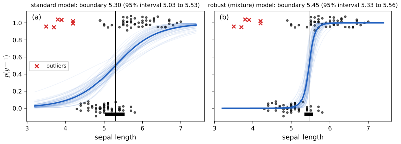
p. 360 The simplest remedy changes the likelihood: with probability \(\pi\) the label is drawn uniformly at random, otherwise it follows the usual model, \[ p(y\given\bm x)=\pi\operatorname{Ber}(y\given0.5)+(1-\pi)\operatorname{Ber}\big(y\given\sigma(\bm w^\T\bm x)\big). \tag{10.99} \] It can be fitted by SGD or by Bayesian inference such as MCMC. The book contaminates the two-class iris data (setosa against versicolor, sepal length) with six versicolor flowers of abnormally low sepal length and compares the standard and robust fits (Figure 10.10).
Filling the gap 10.14: the mixture likelihood is a label-flip model with a bounded loss p. 360, (10.99)
Derivation
Equivalence with label flipping. For \(\tilde y\in\{\pm1\}\) and margin \(m=\tilde ya\), (10.99) gives \(p(y\given\bm x)=\frac\pi2+(1-\pi)\sigma(m)\). A symmetric label-flip model, in which the true label \(t\sim\operatorname{Ber}(\sigma(a))\) is flipped with probability \(\varepsilon\) to give the observed label, has \(p(y\given\bm x)=(1-\varepsilon)\sigma(m)+\varepsilon(1-\sigma(m))=\varepsilon+(1-2\varepsilon)\sigma(m)\). The two are identical with \(\varepsilon=\pi/2\): "replace the label by a fair coin with probability \(\pi\)" is the same as "flip the label with probability \(\pi/2\)".
Bounded loss. The loss of one example is \(\ell(m)=-\log[\varepsilon+(1-2\varepsilon)\sigma(m)]\), which is decreasing in \(m\) with \(\ell(m)\to-\log(1-\varepsilon)\) as \(m\to+\infty\) and \(\ell(m)\to-\log\varepsilon=\log\frac2\pi\) as \(m\to-\infty\). So no example can contribute more than \(\log(2/\pi)\), in contrast to the logistic loss \(\log(1+e^{-m})\approx-m\). For \(\pi=0.1\) the bound is \(\log20=3.0\) (the check gives 2.996).
Vanishing influence. The derivative with respect to the logit is \(\ell'(m)=-\frac{(1-2\varepsilon)\sigma(m)(1-\sigma(m))}{\varepsilon+(1-2\varepsilon)\sigma(m)}\). As \(m\to-\infty\), \(\sigma(m)(1-\sigma(m))\approx e^m\) while the denominator tends to \(\varepsilon>0\), so \(\ell'(m)\to0\) exponentially fast: a point that is badly misclassified exerts no pull on the fit. For the logistic loss \(\ell'(m)=-(1-\sigma(m))\to-1\): the pull stays at its maximum however far the point is. The price is that \(\ell\) is not convex (it flattens for \(m\ll0\)), so the fit may have several local optima and the objective is not guaranteed to be minimised by Newton or IRLS; in the Bayesian treatment one samples \((\bm w,\pi)\) instead.
Numerical results (Figure 10.10). The sampler is a random-walk Metropolis algorithm on (intercept, slope, \(\operatorname{logit}\pi\)) for the centred sepal length with \(\N(0,10^2)\) priors on the coefficients and a \(\operatorname{Beta}(1,9)\) prior on \(\pi\); the proposal covariance is adapted from a warm-up run, 25,000 draws are kept after a burn-in of 5,000 (acceptance rate 0.39). With the six outliers the standard model puts the decision boundary at 5.30 with a 95% credible interval of width 0.51 (5.03 to 5.53); the robust model puts it at 5.45 with width 0.22 (5.33 to 5.56), close to the clean-data value 5.41 (5.30 to 5.54, width 0.24). The posterior median of \(\pi\) is 0.24. This is the pattern described in the book: the robust boundary is close to the one from clean data, and its posterior uncertainty is smaller than for the non-robust model. \(\square\)
10.4.2 Bi-tempered loss
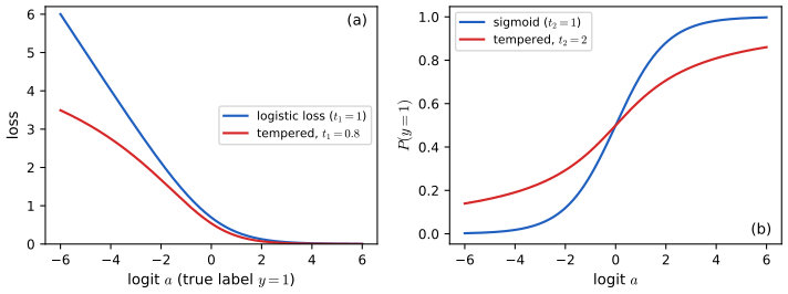
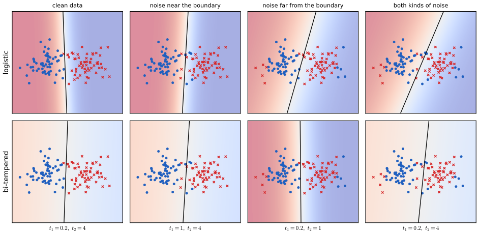
pp. 361–363 The bi-tempered logistic loss of Amid, Warmuth, Anil and Koren (2019) targets two failure modes. (i) Mislabelled points far from the boundary dominate a convex loss; fix: use a bounded loss, obtained by replacing the logarithm in the cross entropy by the tempered logarithm with \(0\le t_1<1\). (ii) Mislabelled points near the boundary need a link with heavier tails than the softmax, so that the model can "look past" the neighbourhood; fix: replace the exponential in the softmax by a tempered exponential with \(t_2>1\). The tempered functions are \[ \log_t(x)=\frac{x^{1-t}-1}{1-t},\qquad \exp_t(x)=\big[1+(1-t)x\big]_+^{1/(1-t)}, \tag{10.103, 10.106} \] both reducing to \(\log\) and \(\exp\) as \(t\to1\). The tempered cross entropy between a target \(\bm y\) and a prediction \(\hat{\bm y}\) is \[ L(\bm y,\hat{\bm y})=\sum_c\Big[y_c\big(\log_{t_1}y_c-\log_{t_1}\hat y_c\big)-\frac1{2-t_1}\big(y_c^{2-t_1}-\hat y_c^{2-t_1}\big)\Big], \tag{10.101} \] which for a one-hot target on class \(c\) is \[ L(c,\hat{\bm y})=-\log_{t_1}\hat y_c-\frac1{2-t_1}\Big(1-\sum_{c'}\hat y_{c'}^{\,2-t_1}\Big). \tag{10.102} \] (The book's (10.100) omits the minus sign of the cross entropy.) The tempered softmax is \(\hat y_c=\exp_{t_2}(a_c-\lambda_{t_2}(\bm a))\) (10.105), with \(\lambda\) the normaliser that solves \(\sum_c\exp_{t_2}(a_c-\lambda)=1\) (10.107), found by bisection or by the fixed-point iteration of Algorithm 10.2.
Algorithm 10.2: computing \(\lambda(\bm a)\) in (10.107), \(t>1\)
Set \(\mu=\max_ca_c\) and \(\bm a\leftarrow\bm a-\mu\bm 1\) (this fixes \(\bm a_0:=\bm a-\mu\bm 1\)). While not converged: \(Z(\bm a)=\sum_c\exp_t(a_c)\); \(\bm a\leftarrow Z(\bm a)^{1-t}\,\bm a_0\). Return \(\lambda=-\log_t(1/Z(\bm a))+\mu\). (As printed, the book's line 6 multiplies the current \(\bm a\) minus \(\mu\bm1\) at every pass, which would subtract \(\mu\) repeatedly; the version that matches the derivation in gap 10.15, and the one that agrees with bisection, keeps the shifted logits \(\bm a_0\) fixed on the right-hand side. Python: tempered_lambda_alg; tempered_softmax uses Newton's method on \(\lambda\), which converges in a few steps and agrees with the algorithm to \(10^{-15}\).)
Filling the gap 10.15: properties of the tempered functions, the loss as a Bregman divergence, and the derivation of Algorithm 10.2 pp. 361–363, (10.101)–(10.107), [AWS19]
Derivation
Tempered functions. \(\log_t\) has derivative \(x^{-t}>0\) and second derivative \(-tx^{-t-1}<0\): increasing and concave. As \(t\to1\), \(\frac{x^{1-t}-1}{1-t}\to\frac{\d}{\d s}x^{s}|_{s=0}=\log x\). For \(t<1\) and \(x\downarrow0\), \(\log_t(x)\to-\frac1{1-t}\): it is bounded below, whereas \(\log\to-\infty\). Solving \(y=\frac{x^{1-t}-1}{1-t}\) for \(x\) gives \(x=[1+(1-t)y]^{1/(1-t)}\), so \(\exp_t\) is the inverse of \(\log_t\) (on \(1+(1-t)y>0\)); the \([\cdot]_+\) sets the value to 0 where the bracket is not positive (for \(t<1\)). For \(t>1\), \(\exp_t(x)=[1+(t-1)(-x)]^{-1/(t-1)}\) decays only polynomially as \(x\to-\infty\), e.g. \(\exp_2(x)=1/(1-x)\), so the tempered softmax has heavy tails: with logits \((0,30)\) and \(t_2=2\) the smaller class gets probability 0.032, whereas the softmax gives less than \(10^{-12}\).
(10.102) from (10.101). For \(\bm y=\bm e_c\) the terms with \(y_k=0\) vanish (\(y_k\log_{t_1}y_k\to0\)), leaving \(\log_{t_1}1-\log_{t_1}\hat y_c-\frac1{2-t_1}(1-\sum_k\hat y_k^{2-t_1})\) and \(\log_{t_1}1=0\).
The loss is a divergence. Let \(F(\bm p)=\sum_k\frac{p_k^{2-t}-p_k}{(1-t)(2-t)}\); then \(F'(p_k)=\log_t p_k\) and \(F''(p_k)=p_k^{-t}>0\), so \(F\) is convex. The Bregman divergence \(D_F(\bm y\|\hat{\bm y})=F(\bm y)-F(\hat{\bm y})-\sum_k\log_t\hat y_k(y_k-\hat y_k)\) simplifies, using \(p\log_tp=\frac{p^{2-t}-p}{1-t}\), to \(D_F=\sum_k\big[y_k\log_ty_k-y_k\log_t\hat y_k-\frac{y_k^{2-t}-\hat y_k^{2-t}}{2-t}\big]+\frac1{2-t}\sum_k(y_k-\hat y_k)\), and the last sum is 0 when both vectors sum to 1. So (10.101) equals \(D_F(\bm y\|\hat{\bm y})\ge0\), with equality iff \(\hat{\bm y}=\bm y\) (strict convexity): it generalises the KL divergence, to which it reduces as \(t_1\to1\).
Boundedness. In (10.102), \(\hat y^{2-t_1}\le\hat y\) because \(2-t_1>1\) and \(\hat y\le1\), so \(\sum_{c'}\hat y_{c'}^{2-t_1}\le1\) and the second term of \(L\) is \(\le0\) (it subtracts a nonnegative number). Hence \(L(c,\hat{\bm y})\le-\log_{t_1}\hat y_c<\frac1{1-t_1}\) for every prediction: the loss is bounded by \(\frac1{1-t_1}\), \(=1.25\) for \(t_1=0.2\) (attained in the limit \(\hat y_c\to0\) with the rest of the mass on one other class; the check gives 1.25).
Algorithm 10.2. Write \(\bm a_0=\bm a-\mu\bm 1\) and look for \(\lambda=\mu+\tilde\lambda\), so \(\sum_c\exp_t(a_{0c}-\tilde\lambda)=1\). Factor the bracket: \(1+(1-t)(a_{0c}-\tilde\lambda)=\big(1-(1-t)\tilde\lambda\big)\big[1+(1-t)\kappa\,a_{0c}\big]\) with \(\kappa=\big(1-(1-t)\tilde\lambda\big)^{-1}\) (positive, since for \(t>1\) and \(\tilde\lambda\ge0\) the bracket \(1+(t-1)\tilde\lambda\) is positive). Raising to the power \(\frac1{1-t}\): \(\exp_t(a_{0c}-\tilde\lambda)=\kappa^{-1/(1-t)}\exp_t(\kappa a_{0c})\). The constraint becomes \(\kappa^{-1/(1-t)}Z(\kappa\bm a_0)=1\), i.e. \(\kappa=Z(\kappa\bm a_0)^{1-t}\). Algorithm 10.2 iterates \(\bm a\leftarrow Z(\bm a)^{1-t}\bm a_0\), whose fixed point is \(\bm a=\kappa\bm a_0\) with exactly this property. Then \(\tilde\lambda=\frac{1-\kappa^{-1}}{1-t}=\frac{1-Z^{-(1-t)}}{1-t}=-\log_t(1/Z)\), because \(\log_t(1/Z)=\frac{Z^{t-1}-1}{1-t}\); this is the returned value \(-\log_t(1/Z(\bm a))+\mu\). The solution of (10.107) exists and is unique because \(\lambda\mapsto\sum_c\exp_t(a_c-\lambda)\) is continuous, strictly decreasing, \(\ge1\) at \(\lambda=\max_ca_c\) and tends to 0 as \(\lambda\to\infty\); it also shows that bisection on \([\max a,\max a+(C^{t-1}-1)/(t-1)]\) is valid, and that Newton's method started at \(\max a\) converges monotonically, the sum being convex and decreasing in \(\lambda\). Numerically, Newton, bisection and Algorithm 10.2 agree to \(10^{-15}\) on random logits for \(t=1.5,2,4\).
Two classes. With logits \((0,a)\), symmetry gives \(P(y=1)>\frac12\) iff \(a>0\) for every \(t_2\): the tempered sigmoid has the same decision boundary as the sigmoid (Figure 10.11b) but different confidence, and a bounded loss for \(t_1<1\) (Figure 10.11a). The objective is no longer convex in \(\bm w\), so a good start (the logistic fit) and a small penalty on \(\bm w\) are used in the code, since without a penalty the weights of a separable data set run off to infinity while the loss tends to 0. \(\square\)
10.5 Bayesian logistic regression *
p. 363 The MLE and MAP estimates are point estimates; with little data, or when a wrong decision is costly, one wants the posterior \(p(\bm w\given\mathcal D)\). Unlike linear regression, it is not available in closed form for logistic regression, because the logistic likelihood is not conjugate to the Gaussian prior. Many approximations exist (see the sequel to the book); the simplest is the Laplace approximation of Section 4.6.8.2.
10.5.1 Laplace approximation
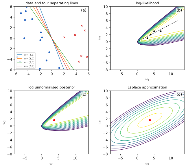
pp. 363–366 The posterior is approximated by a Gaussian centred at the MAP estimate with covariance the inverse Hessian of the negative log posterior there: \(p(\bm w\given\mathcal D)\approx\N(\bm w\given\hat{\bm w},\bm H^{-1})\). The mode is found as in Section 10.2.7 and \(\bm H\) from Section 10.2.3.4. Take the two-dimensional data of Figure 10.13a, which are linearly separable: many lines (four are drawn) classify them perfectly, the log-likelihood surface (b) increases along a ridge towards infinity, so the MLE is at infinity (Result 10.1), and a spherical prior \(\N(\bm 0,\sigma^2\bm I)\) with \(\sigma^2=100\) turns the ridge into a bounded hill (c) whose Laplace approximation is (d). With \(\sigma^2=0\) the MAP is \(\bm w=\bm 0\) and every prediction is \(\frac12\); with \(\sigma^2=\infty\) it is the (infinite) MLE with predictions of exactly 0 or 1.
Filling the gap 10.16: the Laplace approximation, the Monte Carlo predictive and the probit approximation in full pp. 363–367, (10.108)–(10.118)
Derivation
Laplace. Let \(\psi(\bm w)=-\log p(\bm w)-\log p(\mathcal D\given\bm w)=\sum_n[\log(1+e^{a_n})-y_na_n]+\frac1{2\sigma^2}\|\bm w\|^2+\mathrm{const}\), so that \(p(\bm w\given\mathcal D)\propto e^{-\psi(\bm w)}\). At the mode \(\hat{\bm w}\), \(\nabla\psi=\bm 0\) and a second-order Taylor expansion gives \(\psi(\bm w)\approx\psi(\hat{\bm w})+\frac12(\bm w-\hat{\bm w})^\T\bm H(\bm w-\hat{\bm w})\), \(\bm H=\nabla^2\psi(\hat{\bm w})=\bm X^\T\hat{\bm S}\bm X+\sigma^{-2}\bm I\) (sums, not averages: the posterior is for the whole data set). The matrix is positive definite whatever the data, so the Gaussian approximation always exists, even for separable data (gap 10.7). Normalising, \(p(\bm w\given\mathcal D)\approx\N(\hat{\bm w},\bm H^{-1})\). The approximation is exact at the mode by construction, symmetric about it, and can be poor where the posterior is skewed (Figure 10.13: the true posterior is a curved ridge, the Laplace approximation an ellipse). The same expansion gives the normalising constant: \(\int e^{-\psi}\d\bm w\approx e^{-\psi(\hat{\bm w})}(2\pi)^{D/2}|\bm H|^{-1/2}\), the Laplace estimate of the evidence. Numerically, for the data of Figure 10.13 with \(\sigma^2=100\): \(\hat{\bm w}=(3.75,1.63)\), \(\|\hat{\bm w}\|=4.09\), and \(\bm H^{-1}=\begin{pmatrix}13.22&5.37\\5.37&4.11\end{pmatrix}\) (standard deviations 3.64 and 2.03, correlation 0.73).
Predictive distribution. The posterior predictive is \(p(y=1\given\bm x,\mathcal D)=\int\sigma(\bm w^\T\bm x)p(\bm w\given\mathcal D)\,\d\bm w\) (10.108), the average of the sigmoid over the posterior; the plug-in approximation replaces \(p(\bm w\given\mathcal D)\) by a point mass at \(\hat{\bm w}\) (10.109). If \(\bm w\sim\N(\bm m_w,\bm\Sigma)\), the logit \(a=\bm w^\T\bm x\) is a linear function of a Gaussian vector, hence \(a\sim\N(m,v)\) with \(m=\bm x^\T\bm m_w\) and \(v=\bm x^\T\bm\Sigma\bm x\) (10.114, 10.115), and the \(D\)-dimensional integral collapses to the one-dimensional \(\E[\sigma(a)]\), \(a\sim\N(m,v)\). The Monte Carlo estimate (10.110) averages \(\sigma(\bm w_s^\T\bm x)\) over \(S\) posterior draws; its standard error is \(O(S^{-1/2})\). Numerically, with 400,000 draws it agrees with the quadrature value of the integral to 0.001.
Probit approximation. Three steps.
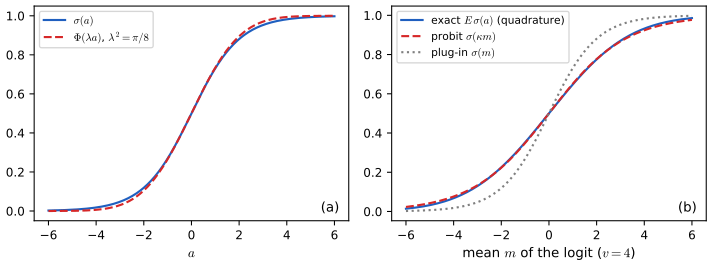
- Sigmoid against the probit. \(\sigma(a)\approx\Phi(\lambda a)\) for the standard normal cdf \(\Phi\). The two functions both equal \(\frac12\) at 0 and are odd about it, and the constant \(\lambda\) is chosen to match slopes at the origin: \(\sigma'(0)=\frac14\) and \(\frac{\d}{\d a}\Phi(\lambda a)|_0=\lambda/\sqrt{2\pi}\), so \(\lambda=\sqrt{2\pi}/4\), \(\lambda^2=\pi/8\) (Figure 10.S3a). The largest difference between the two curves is 0.0177.
- An exact Gaussian integral. For \(a\sim\N(m,v)\), \(\int\Phi(\lambda a)\N(a\given m,v)\,\d a=\Phi\Big(\dfrac m{\sqrt{\lambda^{-2}+v}}\Big)\). Proof: let \(\xi\sim\N(0,1)\) be independent of \(a\). Then \(\Phi(\lambda a)=\Pr(\xi\le\lambda a\given a)\), so the integral equals \(\Pr(\lambda a-\xi\ge0)\). The variable \(\lambda a-\xi\) is Gaussian with mean \(\lambda m\) and variance \(\lambda^2v+1\), so the probability is \(\Phi\big(\lambda m/\sqrt{1+\lambda^2v}\big)=\Phi\big(m/\sqrt{\lambda^{-2}+v}\big)\) (10.111).
- Back to the sigmoid. Using step 1 backwards, \(\Phi\big(\lambda\,u\big)\approx\sigma(u)\) with \(u=m/\sqrt{1+\lambda^2v}=\kappa(v)m\), where \(\kappa(v)=(1+\pi v/8)^{-1/2}\) (10.112). Hence \(p(y=1\given\bm x,\mathcal D)\approx\sigma(\kappa(v)m)\) (10.113).
Consequences. Since \(0<\kappa(v)\le1\), \(|\kappa m|\le|m|\) and \(\sigma(\kappa m)\) is closer to \(\frac12\) than the plug-in \(\sigma(m)\): the Bayesian prediction is less confident, more so for inputs where the posterior variance \(v\) of the logit is large (far from the data). Because \(\kappa>0\), \(\sigma(\kappa m)>\frac12\) iff \(m>0\), so the decision boundary is unchanged and the misclassification rate of "being Bayesian" equals the plug-in's here; only the confidence changes (Figure 10.14). On the data of Figure 10.13 the probit value differs from the exact integral by at most about 0.01 on the probe points (e.g. at \(\bm x=(3,3)\): plug-in 1.000, probit 0.834, exact 0.844, Monte Carlo with \(S=1000\) 0.832; Figure 10.S3b shows the same effect for a single logit variance). The approximation is poorest when \(v\) is large and \(|m|\) moderate, where the Gaussian cdf and the logistic differ in their tails.
Multiclass (10.116–10.118). The generalised probit approximation \(p(y=c\given\bm x,\mathcal D)\approx\softmax\big(\kappa(v_c)m_c\big)_c\) with \(m_c=\bm m_c^\T\bm x\) and \(v_c=\bm x^\T\bm V_{cc}\bm x\) shrinks each logit by its own factor. Unlike the binary case, the arg-max can change: the arg-max of \(\kappa(v_c)m_c\) need not be that of \(m_c\) when the \(v_c\) differ across classes. Example: \(\bm m=(1,0.9,0)\), \(\bm v=(40,0,0)\) gives \(\kappa(40)=0.245\) and shrunken logits \((0.245,0.9,0)\): the plug-in picks class 1, the probit prediction picks class 2 (the book makes the same point, citing Rasmussen and Williams, 2006). \(\square\)
10.5.2 Approximating the posterior predictive
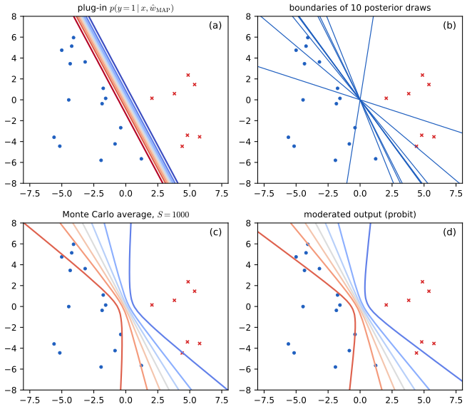
pp. 366–367 In machine learning the quantity of interest is the prediction, not the parameters: \(p(y\given\bm x,\mathcal D)=\int p(y\given\bm x,\bm w)p(\bm w\given\mathcal D)\,\d\bm w\) (10.108). Plug-in (10.109): use \(p(y\given\bm x,\hat{\bm w})\), which ignores posterior uncertainty (Figure 10.14a: parallel contours, no uncertainty about the orientation of the boundary). Monte Carlo (10.110): average \(\sigma(\bm w_s^\T\bm x)\) over \(S\) samples \(\bm w_s\sim p(\bm w\given\mathcal D)\) (Figure 10.14b shows the boundaries of ten samples, c the average): the contours "splay out" away from the data, where many boundaries disagree. Probit (10.113): the deterministic formula \(\sigma(\kappa(v)m)\) of gap 10.16, with \(m=\bm x^\T\hat{\bm w}\), \(v=\bm x^\T\bm H^{-1}\bm x\) (Figure 10.14d), nearly identical to the Monte Carlo average and costing one quadratic form per input.
See also: Bayesian and Probabilistic ML, Sections 4.5.1 and 4.5.2 (Laplace approximation and the predictive distribution) and its variational logistic regression demo.
10.6 Exercises
All three exercises of Chapter 10 (Murphy, 2022, pp. 367–369), restated in my own words, with complete solutions (hidden). A dagger marks the book's own flag for solutions available in its solution material; here every solution is worked independently. Exercise 10.2 refers to a sketch in the book (Figure 10.15a) whose points I re-read from the page, so the error counts there depend on that reading; the reasoning does not.
Exercise 10.1 (gradient and Hessian for multinomial logistic regression). Let \(\mu_{ik}=\softmax(\bm\eta_i)_k\) with \(\bm\eta_i=\bm W^\T\bm x_i\). (a) Show \(\partial\mu_{ik}/\partial\eta_{ij}=\mu_{ik}(\delta_{kj}-\mu_{ij})\) (10.119). (b) Hence show that the gradient of the log-likelihood \(\ell\) is \(\nabla_{\bm w_c}\ell=\sum_i(y_{ic}-\mu_{ic})\bm x_i\) (10.120); hint: use \(\sum_cy_{ic}=1\). (c) Show that the \((c,c')\) block of the Hessian is \(\bm H_{c,c'}=-\sum_i\mu_{ic}(\delta_{c,c'}-\mu_{i,c'})\bm x_i\bm x_i^\T\) (10.121), and hence that the Hessian of the NLL is positive definite.
Solution
(a) With \(Z_i=\sum_je^{\eta_{ij}}\), \(\partial\mu_{ik}/\partial\eta_{ij}=(\delta_{kj}e^{\eta_{ik}}Z_i-e^{\eta_{ik}}e^{\eta_{ij}})/Z_i^2=\mu_{ik}\delta_{kj}-\mu_{ik}\mu_{ij}=\mu_{ik}(\delta_{kj}-\mu_{ij})\).
(b) \(\ell=\sum_i\sum_ky_{ik}\log\mu_{ik}\), so \(\partial\ell/\partial\eta_{ij}=\sum_ky_{ik}\frac1{\mu_{ik}}\mu_{ik}(\delta_{kj}-\mu_{ij})=y_{ij}-\mu_{ij}\sum_ky_{ik}=y_{ij}-\mu_{ij}\). With \(\eta_{ij}=\bm w_j^\T\bm x_i\), \(\nabla_{\bm w_j}\ell=\sum_i(y_{ij}-\mu_{ij})\bm x_i\).
(c) Differentiate \(\partial\ell/\partial\bm w_c=\sum_i(y_{ic}-\mu_{ic})\bm x_i\) with respect to \(\bm w_{c'}^\T\): \(\partial\mu_{ic}/\partial\bm w_{c'}=\mu_{ic}(\delta_{cc'}-\mu_{ic'})\bm x_i\) by (a), so \(\bm H_{c,c'}=-\sum_i\mu_{ic}(\delta_{cc'}-\mu_{ic'})\bm x_i\bm x_i^\T\). The Hessian of the NLL is \(-\bm H\). For a stacked \(\bm v=(\bm u_1,\dots,\bm u_C)\), \(\bm v^\T(-\bm H)\bm v=\sum_i\operatorname{var}_{c\sim\bm\mu_i}[\bm u_c^\T\bm x_i]\ge0\) (see gap 10.9 for the algebra), so the Hessian of the NLL is positive semi-definite. It is positive definite on the clamped parametrisation (\(\bm w_C=\bm 0\)) when \(\operatorname{rank}\bm X=D\); in the unclamped parametrisation it has the \(D\)-dimensional null space \(\{\bm 1\otimes\bm u\}\) (checked numerically: for 3 classes and 3 features the \(9\times9\) Hessian has exactly three zero eigenvalues). So "hence positive definite" in the exercise holds only after clamping one class, which is the form (10.85) that the book uses elsewhere. \(\square\)
Exercise 10.2 (regularising separate terms in 2-D logistic regression) †. The 13 training points of Figure 10.15a (six of class 1 on the left, seven of class 0 on the right of the plane, reproduced below) are fitted with \(p(y=1\given\bm x,\bm w)=\sigma(w_0+w_1x_1+w_2x_2)\). (a) Minimise \(J(\bm w)=-\ell(\bm w,\mathcal D_{\rm train})\) (maximum likelihood): sketch a possible decision boundary; is it unique; how many training errors? (b) Now add \(\lambda w_0^2\) with \(\lambda\) very large. (c) Add \(\lambda w_1^2\) instead. (d) Add \(\lambda w_2^2\) instead. In each case sketch a boundary and count the training errors.
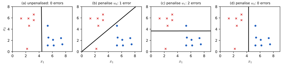
Figure 10.S4 (supplementary). The four fits of Exercise 10.2 on my re-reading of the data of Figure 10.15a (class 1 red crosses, class 0 blue dots): (a) no penalty, (b) \(w_0\) heavily penalised, (c) \(w_1\) heavily penalised, (d) \(w_2\) heavily penalised, with the number of training errors. Original figure; the point coordinates are approximate. Solution
Read from the sketch (grid units), class 1: \((1.3,5.9),(2.4,5.9),(3.2,6.6),(3.2,5.6),(2.5,4.6),(2.2,0.5)\); class 0: \((5.3,4.6),(5.4,2.5),(6.1,2.1),(7.3,2.4),(5.3,1.1),(6.2,1.1),(7.5,1.3)\). Every class-1 point has \(x_1\le3.2\) and every class-0 point \(x_1\ge5.3\): the data are linearly separable by a vertical line.
(a) Because the data are separable, the likelihood is maximised only at infinity (Result 10.1): no finite \(\hat{\bm w}\) exists, and every separating line is a limit of maximum-likelihood-improving fits, so the boundary is not unique; a nearly vertical line between the clusters has 0 errors (the figure shows a numerical solution with a tiny penalty, \(\|\bm w\|\approx120\)).
(b) With \(w_0\) forced to 0 the boundary \(w_1x_1+w_2x_2=0\) passes through the origin, and \(w_1,w_2\) are free. A line through the origin cannot separate the classes: seen from the origin the class-1 points lie at angles \(13^\circ\) (the point \((2.2,0.5)\)) to \(78^\circ\), the class-0 points at \(10^\circ\) to \(41^\circ\), interleaved. The best such line cuts at about \(42^\circ\), putting all class-0 points on one side and misclassifying only the low class-1 point: 1 error in this reading. Hint of the book: with \(x_1=x_2=0\) the model's logit is \(w_0\), so shrinking \(w_0\) forces the probability 1/2 at the origin, i.e. the boundary through it.
(c) With \(w_1\to0\) the logit depends on \(x_2\) only, so the boundary is a horizontal line \(x_2=\mathrm{const}\). The class-1 points have \(x_2\in\{0.5,4.6,5.6,5.9,5.9,6.6\}\) and the class-0 points \(x_2\in\{1.1,1.1,1.3,2.1,2.4,2.5,4.6\}\): no threshold separates them. The best one (between 2.5 and 4.6) misclassifies the class-1 point at height 0.5 and the class-0 point at height 4.6: 2 errors.
(d) With \(w_2\to0\) the boundary is vertical, \(x_1=\mathrm{const}\), which does separate the classes: 0 errors (and, as in (a), the line can be anywhere between \(x_1=3.2\) and \(5.3\) in the limit; with the penalty the solution settles near \(x_1=4.3\)). Moral: the penalty removes the freedom of the weights it touches, so regularising a weight that the boundary needs (here \(w_1\)) hurts, and regularising one it does not need (here \(w_2\)) costs nothing. All four fits were computed by Newton/BFGS (
penalised_fitin the code) with \(\lambda=10^4\) in (b)–(d). \(\square\)Exercise 10.3 (logistic regression against LDA and QDA) †. Train four binary classifiers by maximum likelihood: GaussI (class-conditional \(\N(\bm\mu_c,\bm I)\), uniform \(p(y)\)), GaussX (\(\N(\bm\mu_c,\bm\Sigma_c)\), unrestricted), LinLog (logistic regression on linear features) and QuadLog (logistic regression on linear and quadratic features, including cross terms). Let \(L(M)=\frac1n\sum_i\log p(y_i\given\bm x_i,\hat{\bm\theta},M)\) be the training conditional log-likelihood. For each pair state whether \(L(M)\le L(M')\), \(\ge\), or neither holds for every training set: (a) GaussI, LinLog; (b) GaussX, QuadLog; (c) LinLog, QuadLog; (d) GaussI, QuadLog; (e) is it true in general that \(L(M)>L(M')\) implies \(R(M)<R(M')\), where \(R\) is the training misclassification rate?
Solution
The idea: a generative model with Gaussian class-conditionals has a logistic (or quadratic-logistic) posterior, so it is a member of a discriminative family; the discriminative model maximises the conditional likelihood over that whole family, and so can do no worse on the training set.
(a) For GaussI with uniform \(p(y)\), \(\log\frac{p(y=1\given\bm x)}{p(y=0\given\bm x)}=(\bm\mu_1-\bm\mu_0)^\T\bm x-\frac12(\|\bm\mu_1\|^2-\|\bm\mu_0\|^2)\), a linear logit, so GaussI's conditional likelihood at its fitted \((\hat{\bm\mu}_0,\hat{\bm\mu}_1)\) equals that of one particular linear logistic model. LinLog maximises the conditional likelihood over all linear logits, hence \(L(\text{GaussI})\le L(\text{LinLog})\).
(b) For GaussX the log-odds is \[ \tfrac12\bm x^\T(\bm\Sigma_0^{-1}-\bm\Sigma_1^{-1})\bm x+(\bm\Sigma_1^{-1}\bm\mu_1-\bm\Sigma_0^{-1}\bm\mu_0)^\T\bm x+\mathrm{const}, \] a polynomial of degree 2 in \(\bm x\), representable by QuadLog (linear, square and cross-product features). Hence \(L(\text{GaussX})\le L(\text{QuadLog})\).
(c) Linear features are a subset of linear-plus-quadratic features (set the quadratic weights to 0), so the QuadLog maximum is at least the LinLog maximum: \(L(\text{LinLog})\le L(\text{QuadLog})\).
(d) By (a) and (c), \(L(\text{GaussI})\le L(\text{LinLog})\le L(\text{QuadLog})\), so \(L(\text{GaussI})\le L(\text{QuadLog})\). (Nothing can be said between GaussI and GaussX, or between GaussX and LinLog, in general: they are not nested in the right direction for an inequality valid for every data set.)
(e) No: the log-likelihood rewards confidence and the misclassification rate does not. Counterexample with five training points, labels \((1,1,1,1,0)\). Model A has all logits equal to 0.1: it predicts class 1 everywhere, with errors \(R(A)=\frac15\) and \(L(A)=-0.664\). Model B has logits \((5,5,5,-0.01,0.1)\): it is nearly certain and right on three points and almost indifferent on the other two, where it is wrong; \(R(B)=\frac25\) but \(L(B)=-0.293>L(A)\). So \(L(B)>L(A)\) with \(R(B)>R(A)\). (Training the models for (a)–(d) on 25 random data sets confirmed the orderings (a)–(d) every time.) \(\square\)
Demonstrations
| Page | What it shows | In the notes |
|---|---|---|
| Gradient, bound and Newton steps | Paths of gradient descent, the fixed-matrix bound iteration and Newton/IRLS on the loss surface of the one-feature iris logistic regression, and the NLL gap against the iteration. Presets: 1 gradient descent crawls; 2 Newton in 8 steps; 3 standardised feature; 4 step too large; 5 bound iteration from a far start. | 10.2.6, 10.2.8, gap 10.10 |
| Laplace approximation and the probit predictive | Separable 2-D data, MAP and Laplace posterior for a chosen prior variance, predictive by plug-in, Monte Carlo and probit, with a movable probe point. Presets: 1 probit; 2 plug-in; 3 Monte Carlo; 4 strong prior; 5 flat prior. | 10.5.1, 10.5.2, gap 10.16 |
| Robust logistic regression | Iris sepal length with up to six outliers: standard fit, label-flip mixture and bi-tempered loss, with the loss curves. Presets: 1 standard; 2 mixture; 3 bounded loss; 4 heavy-tailed link; 5 clean data. | 10.4.1, 10.4.2, gap 10.14, gap 10.15 |
The Python code that produces every figure of this page is code/ch10_logistic_regression.py (see the code index). Companion demos: logistic regression, IRLS, variational logistic regression.
Notes on the book
Points where the book is imprecise or wrong
- (10.25), strict convexity. The Hessian \(\frac1N\bm X^\T\bm S\bm X\) is positive definite only if \(\bm X\) has full column rank (e.g. not with duplicated features or \(N<D\)); \(\mu_n>0\) alone gives positive semi-definiteness and the book's chain \(\|\bm v^\T\bm X^\T\bm S^{1/2}\|^2>0\) needs \(\bm X\bm v\ne\bm 0\) (gap 10.3).
- Exercise 10.1c and Section 10.3.2.4. The \(CD\times CD\) Hessian of the unclamped softmax regression is not positive definite: adding the same vector to every class's weights leaves the likelihood unchanged, giving a \(D\)-dimensional null space. It is positive definite after clamping one class (gap 10.9); the book itself relies on this in Section 10.3.5.
- (10.82), sign. With \(\bm g_t=\bm X^\T(\bm y-\bm\mu_t)\) (the gradient of the log-likelihood) the bound-optimisation update is \(\bm w_{t+1}=\bm w_t+4(\bm X^\T\bm X)^{-1}\bm g_t\); the printed minus sign would move uphill. The comparison (10.83) with Newton's step is consistent only if \(\bm g_t\) is the gradient of the NLL there (Section 10.3.4).
- Fisher scoring (end of Section 10.2.6). For logistic regression the Hessian does not depend on the labels, so its expectation is itself, and Fisher scoring is identical to Newton's method and to IRLS. The Fisher information \(\bm X^\T\bm S(\bm w)\bm X\) depends on \(\bm w\) and cannot be precomputed once; the book's remark applies to non-canonical links (gap 10.6).
- (10.100), missing minus sign. The cross entropy is \(H_{\rm ce}(\bm y,\hat{\bm y})=-\sum_cy_c\log\hat y_c\), as in (10.59); (10.100) omits the sign.
- (10.47), the constant in \(\lambda=1/C\). For the average NLL and the prior \(\N(\bm 0,C\bm I)\) the penalty is \(\frac1{2CN}\|\bm w\|^2\), i.e. \(\lambda=1/(2CN)\) in (10.47); the same factor 2 appears in (10.88)–(10.89), where the stationarity condition is \(\sum_n(\bm y_n-\bm\mu_n)\otimes\bm x_n=2\lambda\bm w\) for the penalty \(\lambda\|\bm w\|^2\) (the conclusion \(\sum_c\hat{\bm w}_c=\bm 0\) is unaffected) (gap 10.7, gap 10.11).
- Section 10.3.5, sum-to-zero. The property holds for the penalised coordinates only; with an unpenalised bias the biases remain unidentified up to a common constant (gap 10.11).
- (10.79), the inequality. It should read \(\succeq\); equality is attained, so \(\succ\) is not generally true.
- Section 10.2.4, "will always converge". SGD on the logistic NLL converges to the MLE for non-separable data; for separable data there is no MLE and the iterates diverge in norm (Result 10.1), so "even if the data is not linearly separable" is the only case in which "always converges" is right.
- Dimensions of \(\bm W\). Section 10.3 defines \(\bm W\) as \(C\times D\), Section 10.3.2.3 as \(D\times C\) (with the gradient (10.68) as a \(D\times C\) matrix). The notes use \(D\times C\) from (10.67) on.
- Algorithm 10.2, line 6. The update \(\bm a:=Z(\bm a)^{1-t}(\bm a-\mu\bm1)\) re-subtracts \(\mu\) from the current iterate at each pass; the correct fixed-point iteration is \(\bm a\leftarrow Z(\bm a)^{1-t}\bm a_0\) with the shifted logits \(\bm a_0=\bm a-\mu\bm1\) held fixed (gap 10.15).
References
- Murphy, K. P. (2022). Probabilistic Machine Learning: An Introduction. MIT Press, Cambridge, MA. Chapter 10, pp. 339–369. probml.github.io/pml-book/book1.html.
- Albert, A. and Anderson, J. A. (1984). On the existence of maximum likelihood estimates in logistic regression models. Biometrika, 71(1), 1–10.
- Amid, E., Warmuth, M. K., Anil, R. and Koren, T. (2019). Robust bi-tempered logistic loss based on Bregman divergences. Advances in Neural Information Processing Systems, 32.
- Böhning, D. (1992). Multinomial logistic regression algorithm. Annals of the Institute of Statistical Mathematics, 44(1), 197–200.
- Bishop, C. M. (2006). Pattern Recognition and Machine Learning. Springer, New York.
- Fisher, R. A. (1936). The use of multiple measurements in taxonomic problems. Annals of Eugenics, 7(2), 179–188.
- Hastie, T., Tibshirani, R. and Friedman, J. (2009). The Elements of Statistical Learning, 2nd edition. Springer, New York.
- Novikoff, A. B. J. (1962). On convergence proofs on perceptrons. Proceedings of the Symposium on the Mathematical Theory of Automata, 12, 615–622.
- Rasmussen, C. E. and Williams, C. K. I. (2006). Gaussian Processes for Machine Learning. MIT Press, Cambridge, MA.
- Robbins, H. and Monro, S. (1951). A stochastic approximation method. Annals of Mathematical Statistics, 22(3), 400–407.
- Rosenblatt, F. (1958). The perceptron: a probabilistic model for information storage and organization in the brain. Psychological Review, 65(6), 386–408.
- Soudry, D., Hoffer, E., Nacson, M. S., Gunasekar, S. and Srebro, N. (2018). The implicit bias of gradient descent on separable data. Journal of Machine Learning Research, 19(70), 1–57.
- Spiegelhalter, D. J. and Lauritzen, S. L. (1990). Sequential updating of conditional probabilities on directed graphical structures. Networks, 20(5), 579–605.
The numerical statements in the text (the gradient and Hessian formulas, the rank condition for strict convexity, the non-separability of the iris two-feature problem, the equality of Newton and IRLS, the penalised fits against a standard library, the perceptron mistake bound, the rate of SGD, the Bohning bound and the monotone bound iteration, the sum-to-zero property, the tempered functions and Algorithm 10.2, the Laplace covariance, the probit and Monte Carlo predictives and the numerical answers to the exercises) were confirmed numerically.