Generative adversarial networks
A generative adversarial network (GAN) fits an implicit generative model, a generator network \(\bm x=G_{\bm\theta}(\bm z)\) whose output density cannot be evaluated, by learning from a comparison of its samples with the data. The comparison is carried out by a second network, the discriminator or critic, trained on class probabilities, on a lower bound of an \(f\)-divergence, on a difference of expectations (Wasserstein, MMD) or on moments; the generator then descends the learned comparison. These notes prove the identities behind each choice, work out what gradient descent on the two-player game does (it circles, spirals or converges depending on the update rule and on regularisation), and reproduce the chapter's figures, including the mode collapse of a GAN trained on sixteen Gaussians, with small networks on a CPU.
Ch. 1 Introduction Ch. 2 Probability Ch. 3 Statistics Ch. 4 Graphical models Ch. 5 Information theory Ch. 6 Optimisation Ch. 7 Inference algorithms Ch. 8 Gaussian filtering Ch. 9 Message passing Ch. 10 Variational inference Ch. 11 Monte Carlo Ch. 12 MCMC Ch. 13 Sequential Monte Carlo Ch. 14 Predictive models Ch. 15 GLMs Ch. 16 Deep networks Ch. 17 Bayesian neural networks Ch. 18 Gaussian processes Ch. 19 Beyond iid Ch. 20 Generative models Ch. 21 VAEs Ch. 22 Autoregressive models Ch. 23 Normalizing flows Ch. 24 Energy-based models Ch. 25 Diffusion models Ch. 26 GANs Ch. 27 Discovery methods Ch. 28 Latent factor models Ch. 29 State-space models Ch. 30 Graph learning Ch. 31 Nonparametric Bayes Ch. 32 Representation learning Ch. 33 Interpretability Ch. 34 Decision making Ch. 35 Reinforcement learning Ch. 36 Causality
How to read these notes
They follow the book. Sections carry the book's numbers, and equations the book numbers keep their numbers, e.g. \((26.25)\); equations without a number are steps the book skips. Sections from the online supplement are labelled supplement and placed where the book refers to them (the supplement's Chapter 26 has no content of its own, see S26).
Filling the gaps. Wherever the book writes "it can be shown", quotes a result from the literature, or leaves a step to the reader, an orange Filling the gap box gives the full argument. Proofs start hidden: open one with its bar, or use the buttons below. Results already proved elsewhere on the site (the optimal discriminator and the Jensen–Shannon divergence, the Kantorovich–Rubinstein duality, the score-function and reparameterisation estimators, the bilinear game) are stated and linked, and the boxes spend their space on what this chapter adds: the other proper scoring rules, the conjugates of Table 26.2, the exact gradient of each generator loss at the optimal discriminator, the exact radius law of simultaneous and alternating updates in DiracGAN and the effect of a gradient penalty, and the BiGAN optimum.
Figures, scale and demonstrations. Every computed figure is reproduced by the Python code (numpy, scipy and PyTorch on one CPU thread; the figures of the notes take about three minutes in all). Figures 26.2, 26.9 to 26.18 are diagrams, photographs of trained large models or results of GPU-scale training and are not reproduced (the module docstring gives the reason for each). Figure 26.1 is redrawn from computed data, Figures 26.3 to 26.8 are reproduced with small stand-ins described in the captions, and six figures marked (own) go beyond the book. Three interactive demonstrations are linked where their topics arise.
Main reference
K. P. Murphy, Probabilistic Machine Learning: Advanced Topics, MIT Press (2023; online draft of December 2025), Chapter 26, pages 893–924, written by Mihaela Rosca, Shakir Mohamed and Balaji Lakshminarayanan (book page: probml.github.io/pml-book/book2.html), and the supplementary material, Chapter 26, pages 207–210. Section, equation, figure and algorithm numbers below refer to this book.
Companion courses
The deep-learning course treats the same game at an elementary level: the optimal discriminator, the Jensen–Shannon objective, the bilinear game, the non-saturating loss, why JS cannot see distances, the Wasserstein distance in one dimension and its duality, the conditional optimum and cycle consistency. In this volume, Section 6.3.4–6.3.5 proves the score-function and reparameterisation estimators, gap 6.25 the Kantorovich duality, Section 20.4.2 uses MMD and the Fréchet distance to evaluate generators and Chapter 21 is the likelihood-based counterpart. Volume 1 has logistic regression and kernels.
What this chapter adds: the other proper scoring rules of Table 26.1 and the divergence each one optimises (Brier: a Pearson-type \(\chi^2\); hinge: total variation; exponential: Hellinger), the conjugates and optimal critics of Table 26.2 (and the fact that its JSD row is \(2\,\JSD\)), the reason a restricted critic gives a lower bound that need not decrease with the divergence, the exact gradients of the saturating and non-saturating generator losses at the optimal discriminator, the exact dynamics of DiracGAN (conserved radius, radius law of simultaneous updates, invariant ellipse of alternating updates, stability with a penalty), the conditional and BiGAN optima, and experiments on the sixteen-mode problem.
The chapter at a glance
- 26.1 Implicit models and the density of a push-forward (gap 26.1).
- 26.2 Learning by comparison: the optimal discriminator and the JSD (gap 26.2); other scoring rules (26.3); the \(f\)-divergence bound, Table 26.2 and why bounds can mislead (26.4); Wasserstein critics (26.5); MMD and moment matching (26.6); disjoint supports (26.7).
- 26.3 The saturating and non-saturating gradients at the optimal discriminator (gap 26.8); the reparameterisation gradient of the generator (26.9); mode collapse experiments; DiracGAN and its stability (26.10, 26.11).
- 26.4–26.7 Conditional GANs (gap 26.12); BiGAN (26.13); self-attention, spectral normalisation and gradient penalties (26.14); cycle consistency (26.15).
Notation. \(p^*\) is the data density, \(q(\bm z)\) the latent distribution, \(G_{\bm\theta}\) the generator, \(q_{\bm\theta}\) the distribution of \(G_{\bm\theta}(\bm z)\), \(D_{\bm\phi}\) the discriminator or critic, \(m=\tfrac12(p^*+q_{\bm\theta})\) the mixture, \(\sigma\) the logistic sigmoid. Densities are with respect to a reference measure (Lebesgue measure on \(\R^d\) unless stated).
Prerequisites. Chapters 5 and 6 of the book (KL divergence, optimisation, gradient estimators) and Chapters 17 and 20 of Volume 1 or the deep-learning course.
26.1 Introduction
pp. 893–894 A prescribed (explicit) probabilistic model specifies a log-likelihood \(\log q_{\bm\theta}(\bm x)\); an implicit model specifies only a stochastic procedure that produces data. The implicit models of this chapter are latent-variable models without an observation model, \[ \bm x=G_{\bm\theta}(\bm z'),\quad \bm z'\sim q(\bm z), \tag{26.1} \] \[ q_{\bm\theta}(\bm x)=\frac{\partial}{\partial x_1}\cdots\frac{\partial}{\partial x_d}\int_{\{G_{\bm\theta}(\bm z)\le\bm x\}}q(\bm z)\,\d\bm z, \tag{26.2} \] with \(G_{\bm\theta}:\R^m\to\R^d\), a differentiable simulator. (26.2) says that \(q_{\bm\theta}\) is the derivative of the distribution function of \(G_{\bm\theta}(\bm z)\). When \(m=d\) and \(G_{\bm\theta}\) is invertible this is the change-of-variables rule used by normalising flows (Chapter 23); for \(d>m\) with a deep network the set \(\{G_{\bm\theta}(\bm z)\le\bm x\}\) cannot be characterised and the integral is intractable, so there is no usable likelihood and learning must use only samples: likelihood-free or simulation-based inference, of which approximate Bayesian computation is the other main family (the book's Section 13.6.5).
Filling the gap 26.1: when (26.2) is a density, and what it is when \(d>m\) pp. 893–894, (26.1)–(26.2)
Proof
The law always exists. For any measurable \(G\), \(q_{\bm\theta}(A)=q(G^{-1}(A))\) is a probability measure on \(\R^d\) (the push-forward), and its distribution function is \(F(\bm x)=\Pr(G(\bm Z)\le\bm x)=\int_{\{G(\bm z)\le\bm x\}}q(\bm z)\d\bm z\), the integral in (26.2). The mixed derivative \(\partial^dF/\partial x_1\cdots\partial x_d\) is the density of \(q_{\bm\theta}\) when that measure has a density; otherwise (26.2) is not a function.
\(m=d\), \(G\) a \(C^1\) bijection with nonvanishing Jacobian. For a Borel set \(A\), the change of variables \(\bm z=G^{-1}(\bm x)\) gives \(\int_{G^{-1}(A)}q(\bm z)\d\bm z=\int_Aq(G^{-1}(\bm x))\,|\det J_{G^{-1}}(\bm x)|\d\bm x\), so \[ q_{\bm\theta}(\bm x)=q\big(G^{-1}(\bm x)\big)\,\big|\det J_G(G^{-1}(\bm x))\big|^{-1}. \] For example \(G(z)=z^3\), \(z\sim\N(0,1)\) has \(q_\theta(x)=\varphi(x^{1/3})/(3|x|^{2/3})\), which is integrable (infinite at 0); the derivative of \(F(x)=\Phi(x^{1/3})\) agrees with this.
\(m<d\): no density. If \(G\) is \(C^1\) and \(m<d\), the image \(G(\R^m)\) has Lebesgue measure zero in \(\R^d\) (it is the image of a lower-dimensional manifold; a \(C^1\) map from \(\R^m\) to \(\R^d\) with \(m<d\) maps every set to a null set, a special case of Sard's lemma). The measure \(q_{\bm\theta}\) puts all its mass on this null set, so it is singular with respect to Lebesgue measure and has no density: \(\log q_{\bm\theta}(\bm x)\) is undefined (for a linear \(G(z)=\bm az\) the sample covariance has rank 1, confirmed numerically). So the book's statement that the generating procedure "defines a valid density on the output space" holds for \(m\ge d\) with a Jacobian of full row rank almost everywhere (then, by the coarea formula, \(q_{\bm\theta}(\bm x)=\int_{G^{-1}(\bm x)}q(\bm z)\,[\det(J_GJ_G^\T)]^{-1/2}\d\mathcal H^{m-d}(\bm z)\)); in the case the chapter actually cares about, \(d>m\), the object is a measure, not a density, and only samples are available. This is also why the divergences of Section 26.2 must be estimated from samples.
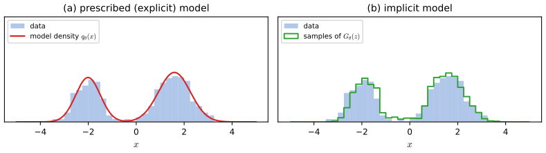
See also: why an implicit model has no usable likelihood (deep-learning course) and likelihood-free inference in Chapter 10.
26.2 Learning by comparison
pp. 894–895 Maximum likelihood minimises \(\Dkl(p^*\|q_{\bm\theta})\) (Section 5.1.6), which needs \(q_{\bm\theta}(\bm x)\). For an implicit model we need training criteria that use only samples from \(q_{\bm\theta}\) and from \(p^*\): a two-sample comparison. The book organises them as in its Figure 26.2 (a tree of approaches: differences, i.e. integral probability metrics and moment matching; ratios, i.e. class-probability estimation and \(f\)-divergences), which is a diagram and is not reproduced.
26.2.1 Guiding principles
p. 895 We want a criterion \(D(p^*,q)\) with (1) \(\argmin_qD(p^*,q)=p^*\), (2) evaluable from samples alone, (3) cheap. Every divergence or distance satisfies (1) because \[ D(p^*,q)\ge0,\qquad D(p^*,q)=0\iff p^*=q. \tag{26.3} \] KL fails (2) and the Wasserstein distance fails (3). The remedy is a comparison model (discriminator, critic) \(D_{\bm\phi}\) and a functional \(F\) with \[ D(p^*,q)=\argmax_DF(D,p^*,q),\tag{26.4} \] more exactly \(D(p^*,q)=\max_DF(D,p^*,q)\): the divergence is the value of the inner problem (and the critic is its argmax). Writing \(F\) as a difference of expectations, \[ F(D_{\bm\phi},p^*,q_{\bm\theta})=\E_{p^*(\bm x)}f(\bm x,\bm\phi)+\E_{q_{\bm\theta}(\bm x)}g(\bm x,\bm\phi)=\E_{p^*}f(\bm x,\bm\phi)+\E_{q(\bm z)}g(G_{\bm\theta}(\bm z),\bm\phi)\approx\frac1N\sum_{i=1}^Nf(\hat{\bm x}_i,\bm\phi)+\frac1M\sum_{i=1}^Mg(G_{\bm\theta}(\hat{\bm z}_i),\bm\phi), \tag{26.5--26.7} \] makes it computable by Monte Carlo from samples \(\hat{\bm x}_i\sim p^*\) and \(\hat{\bm z}_i\sim q\) (the book's (26.4) writes "arg max" where the value, a "max", is meant; see Notes on the book). The four instances of \(f\) and \(g\) are class-probability estimation (26.2.2), bounds on \(f\)-divergences (26.2.3), integral probability metrics (26.2.4) and moment matching (26.2.5).
26.2.2 Density ratio estimation using binary classifiers
pp. 896–898 Label data \(y=1\) and model samples \(y=0\) with equal probability. By Bayes' rule a classifier that outputs \(D(\bm x)=\Pr(y=1\given\bm x)\) encodes the density ratio, since \(D/(1-D)=p^*(\bm x)\Pr(y=1)/(q_{\bm\theta}(\bm x)\Pr(y=0))\): \[ \frac{p^*(\bm x)}{q_{\bm\theta}(\bm x)}=\frac{D(\bm x)}{1-D(\bm x)} \tag{26.8} \] (the book cites the trick of its Section 2.7.5; gap 10.21 shows that a classifier's logit is the log density ratio). Any proper scoring rule can be used to learn \(D_{\bm\phi}\); for the Bernoulli log-loss, \[ \max_{\bm\phi}\ \E_{p(\bm x\given y)p(y)}\big[y\log D_{\bm\phi}(\bm x)+(1-y)\log(1-D_{\bm\phi}(\bm x))\big]=\max_{\bm\phi}\ \tfrac12\E_{p^*}\log D_{\bm\phi}(\bm x)+\tfrac12\E_{q_{\bm\theta}}\log(1-D_{\bm\phi}(\bm x)) \tag{26.9--26.10} \] (the book's (26.9) writes \(V(q_{\bm\theta},p^*)=\argmax_{\bm\phi}\ldots\); \(V\) is the maximal value). The maximiser over all functions is \[ D^*(\bm x)=\frac{p^*(\bm x)}{p^*(\bm x)+q_{\bm\theta}(\bm x)} \tag{26.11} \] and substituting it gives \[ V^*(q_{\bm\theta},p^*)=\tfrac12\E_{p^*}\log\frac{p^*}{p^*+q_{\bm\theta}}+\tfrac12\E_{q_{\bm\theta}}\log\frac{q_{\bm\theta}}{p^*+q_{\bm\theta}}=\JSD(p^*,q_{\bm\theta})-\log2, \tag{26.12--26.15} \] \[ \JSD(p^*,q_{\bm\theta})=\tfrac12\Dkl\big(p^*\,\|\,\tfrac{p^*+q_{\bm\theta}}2\big)+\tfrac12\Dkl\big(q_{\bm\theta}\,\|\,\tfrac{p^*+q_{\bm\theta}}2\big). \tag{26.16} \] A classifier thus turns the intractable divergence into an optimisation problem solvable from samples. The generator then minimises the learned divergence, \(\min_{\bm\theta}\JSD=\min_{\bm\theta}V^*+\log2\) (26.17)–(26.18); since the optimal \(D^*\) is unavailable, one solves the min-max problem \[ \min_{\bm\theta}\max_{\bm\phi}\ \tfrac12\E_{p^*(\bm x)}[\log D_{\bm\phi}(\bm x)]+\tfrac12\E_{q(\bm z)}[\log(1-D_{\bm\phi}(G_{\bm\theta}(\bm z)))], \tag{26.19--26.20} \] the original GAN of Goodfellow et al. (2014). Gap 26.2 proves (26.11) to (26.16) with the properties of the JSD that the chapter uses. Other proper scoring rules (Table 26.1) lead to other divergences (gap 26.3).
Filling the gap 26.2: the optimal discriminator, (26.11)–(26.16), and the range of the JSD pp. 896–898
Proof
Optimal discriminator. Take densities \(p,q\) with respect to a common reference measure. For fixed \(\bm x\), maximise \(\varphi(D)=\tfrac12p\log D+\tfrac12q\log(1-D)\) over \(D\in(0,1)\). It is strictly concave, \(\varphi'(D)=\tfrac{p}{2D}-\tfrac{q}{2(1-D)}\) vanishes at \(D=p/(p+q)\), and the pointwise maximiser is a maximiser of the integral over all measurable \(D\) (where \(p+q=0\) the value of \(D\) is irrelevant). This is (26.11); the density ratio (26.8) follows.
The value. With \(m=\tfrac12(p+q)\) we have \(p/(p+q)=p/(2m)\), so \(\log\frac p{p+q}=\log\frac pm-\log2\) and likewise for \(q\): \[ V^*=\tfrac12\E_p\log\tfrac pm+\tfrac12\E_q\log\tfrac qm-\tfrac12\log2-\tfrac12\log2=\JSD(p,q)-\log2, \] (26.12)–(26.15). (The same computation without the weights \(\tfrac12\) is in the deep-learning course.)
Range of the JSD. (i) \(\JSD\ge0\) with equality iff \(p=q\): both terms are KL divergences, so they are non-negative, and both vanish iff \(p=m\) and \(q=m\), i.e. \(p=q\). (ii) \(\JSD\le\log2\): \(m\ge p/2\) gives \(\log(p/m)\le\log2\) and so \(\Dkl(p\|m)\le\log2\); same for \(q\). Equality needs \(p/m=2\) \(p\)-almost everywhere and \(q/m=2\) \(q\)-almost everywhere, i.e. \(q=0\) where \(p>0\) and \(p=0\) where \(q>0\): the supports are disjoint (\(p\perp q\)). (iii) \(\sqrt{\JSD}\) is a metric (Endres and Schindelin, 2003), so \(\JSD\) is symmetric and its square root satisfies the triangle inequality.
Consequences for the game. For fixed \(q_{\bm\theta}\), \(\max_DV(D,q_{\bm\theta})=\JSD(p^*,q_{\bm\theta})-\log2\ge-\log2\), with equality iff \(q_{\bm\theta}=p^*\) by (i). Hence \(\min_{\bm\theta}\max_DV=-\log2\) is attained at \(q_{\bm\theta}=p^*\) when the generator can represent \(p^*\), and only there. Numerical example (checked on a grid): \(p^*=0.4\,\N(-1,0.8^2)+0.6\,\N(1.5,0.6^2)\), \(q=\N(0.3,1.2^2)\) give \(V^*=-0.6434\) and so \(\JSD=0.0498\).
See also: the generator objective is a Jensen–Shannon divergence and what that result does not say (deep-learning course).
p. 897, Table 26.1 Table 26.1 lists the proper scoring rules that can be maximised instead of the Bernoulli rule (with \(D\in[0,1]\)): Brier \(-\E_{p^*}(1-D)^2-\E_{q}D^2\); exponential \(-\E_{p^*}\sqrt{(1-D)/D}-\E_{q}\sqrt{D/(1-D)}\); misclassification \(-\E_{p^*}\mathbb I[D\le\tfrac12]-\E_{q}\mathbb I[D>\tfrac12]\); hinge (on the logit \(t=\log\frac D{1-D}\)) \(-\E_{p^*}\max(0,1-t)-\E_{q}\max(0,1+t)\); spherical \(\E_{p^*}\alpha D+\E_{q}\alpha(1-D)\) with \(\alpha=(1-2D+2D^2)^{-1/2}\). The Brier score underlies the least-squares GAN (Mao et al., 2017), the hinge loss is popular in large GANs (Miyato et al., 2018; Brock et al., 2019).
Filling the gap 26.3: which divergence each scoring rule optimises (Brier, exponential, hinge) pp. 897–898, Table 26.1
Proof
Work pointwise in \(\bm x\) with \(p=p^*(\bm x)\), \(q=q_{\bm\theta}(\bm x)\), and maximise the integrand over \(D\) (or over the logit \(t\)); the optimal value is then the integral of the pointwise maxima.
Brier. \(-p(1-D)^2-qD^2\) is concave in \(D\) with derivative \(2p(1-D)-2qD=0\) at \(D^*=p/(p+q)\): the same optimal discriminator as the log-loss (that is what proper means: the expected score is maximised by reporting the true class probability). The maximum is \(-\frac{pq^2+qp^2}{(p+q)^2}=-\frac{pq}{p+q}\). Using \(4pq=(p+q)^2-(p-q)^2\), \[ V^*_{\rm Brier}=-\int\frac{pq}{p+q}=-\frac12+\frac14\int\frac{(p-q)^2}{p+q}=-\frac12+\frac12\chi^2\big(p\,\|\,\tfrac{p+q}2\big), \] because \(\chi^2(p\|m)=\int\frac{(p-m)^2}{m}=\frac12\int\frac{(p-q)^2}{p+q}\). So the Brier game minimises a Pearson \(\chi^2\) divergence (to the mixture, the triangular discrimination), as the book states.
Exponential. \(-p\sqrt{(1-D)/D}-q\sqrt{D/(1-D)}\), with \(u=\sqrt{(1-D)/D}\), equals \(-pu-q/u\) and is maximised at \(u=\sqrt{q/p}\), i.e. again \(D^*=p/(p+q)\), with value \(-2\sqrt{pq}\). Hence \(V^*_{\rm exp}=-2\int\sqrt{pq}=-2(1-H^2(p,q))\) with \(H^2=\tfrac12\int(\sqrt p-\sqrt q)^2\) the squared Hellinger distance: the exponential rule optimises the Hellinger distance.
Hinge. Maximise \(-p(1-t)_+-q(1+t)_+\) over \(t\in\R\). For \(t\in[-1,1]\) the objective is \(-(p+q)+(p-q)t\), increasing in \(t\) if \(p>q\); for \(t\ge1\) it equals \(-q(1+t)\), decreasing; for \(t\le-1\) it equals \(-p(1-t)\), increasing in \(t\). So \(t^*=\sgn(p-q)\) and the maximum is \(-2\min(p,q)\); integrating, \(V^*_{\rm hinge}=-2\int\min(p,q)=-2+2\,\TV(p,q)\) since \(\int\min(p,q)=1-\TV\). The hinge rule therefore optimises the total variation distance, matching the book's remark. Unlike the three rules above, the optimal hinge critic is not the log odds: it saturates at \(\pm1\) and carries no information on the size of the ratio. The misclassification rule is piecewise constant in the parameters and gives no gradient.
Check. On the grid example of gap 26.2 the maxima equal \(-0.5+\frac12\chi^2(p\|m)\) (Brier), and \(-2+2\TV=-1.4545\) (hinge); pointwise brute-force maximisation over \(t\) confirms \(t^*=\sgn(p-q)\).
26.2.3 Bounds on f-divergences
pp. 898–900 For a convex \(f\) with \(f(1)=0\) the \(f\)-divergence is \[ D_f[p^*\|q_{\bm\theta}]=\int q_{\bm\theta}(\bm x)\,f\!\Big(\frac{p^*(\bm x)}{q_{\bm\theta}(\bm x)}\Big)\d\bm x, \tag{26.21} \] which contains KL, reverse KL, the Jensen–Shannon divergence and Pearson's \(\chi^2\) (Table 26.2 below; see also the book's Section 2.7.1). It needs both densities, so one uses a variational lower bound. Let \(f^\dagger(t)=\sup_u\,\{ut-f(u)\}\) be the convex conjugate (gap 6.17); since \(f=f^{\dagger\dagger}\) for convex lower semicontinuous \(f\), \[ D_f=\int q_{\bm\theta}\sup_{t}\Big\{t\frac{p^*}{q_{\bm\theta}}-f^\dagger(t)\Big\}=\int\sup_{t}\big\{p^*t-q_{\bm\theta}f^\dagger(t)\big\}\ \ge\ \sup_{t\in\mathcal T}\ \E_{p^*}[t(\bm x)]-\E_{q_{\bm\theta}}[f^\dagger(t(\bm x))], \tag{26.22--26.25} \] where \(t:\mathcal X\to\R\) is a function (the critic) and \(\mathcal T\) a family such as the functions a network can express. The right side is of the form (26.5) and is estimated from samples. Replacing \(t\) by the critic \(D_{\bm\phi}\) gives the \(f\)-GAN (Nowozin et al., 2016): \[ \min_{\bm\theta}D_f(p^*,q_{\bm\theta})\ge\min_{\bm\theta}\max_{\bm\phi}\ \E_{p^*}[D_{\bm\phi}(\bm x)]-\E_{q(\bm z)}[f^\dagger(D_{\bm\phi}(G_{\bm\theta}(\bm z)))]. \tag{26.26--26.27} \] Table 26.2 lists, for four choices of \(f\), the conjugate and the optimal critic as a function of the density ratio \(r=p^*/q_{\bm\theta}\). There is an equivalence between scoring rules and \(f\)-divergence bounds (Reid and Williamson, 2011): the optimal critic is in both cases a function of the density ratio.
| Divergence | \(f(u)\) | \(f^\dagger(t)\) | optimal critic \(t^*=f'(r)\) |
|---|---|---|---|
| KL \(\Dkl(p^*\|q_{\bm\theta})\) | \(u\log u\) | \(e^{t-1}\) | \(1+\log r\) |
| reverse KL \(\Dkl(q_{\bm\theta}\|p^*)\) | \(-\log u\) | \(-1-\log(-t)\), \(t<0\) | \(-1/r\) |
| "JSD" (equals \(2\,\JSD\)) | \(u\log u-(u+1)\log\frac{u+1}2\) | \(-\log(2-e^t)\), \(t<\log2\) | \(\log\frac{2r}{1+r}\) |
| Pearson \(\chi^2\) | \((u-1)^2\) | \(\tfrac14t^2+t\) | \(2(r-1)\) |
Filling the gap 26.4: the bound (26.25), Table 26.2, and why a restricted critic gives a bound that need not follow the divergence pp. 898–900, (26.22)–(26.27), Table 26.2
Proof
The bound and its equality case. Let \(f\) be convex, lower semicontinuous, \(f(1)=0\). For each \(u\) in the domain and \(t\) in that of \(f^\dagger\), \(f(u)\ge ut-f^\dagger(t)\) (Fenchel–Young), with equality iff \(t\in\partial f(u)\). Taking \(u=r(\bm x)\) and any function \(t(\bm x)\), multiplying by \(q_{\bm\theta}(\bm x)\) and integrating gives \(D_f\ge\E_{p^*}t-\E_{q_{\bm\theta}}f^\dagger(t)\) for every critic, hence for the supremum over \(\mathcal T\), which is (26.25). Equality holds iff \(t(\bm x)\in\partial f(r(\bm x))\) almost everywhere, i.e. \(t^*(\bm x)=f'(r(\bm x))\) when \(f\) is differentiable: the optimal critic in the last column of Table 26.2. So the interchange of the supremum and the integral in (26.24) is justified by exhibiting the maximiser \(t^*\). Where \(q_{\bm\theta}=0\) and \(p^*>0\) the integrand of (26.21) is defined by the slope of \(f\) at infinity (\(\infty\) for KL), which the book glosses over; (26.24) then needs \(t\) to be allowed to tend to the boundary of the domain of \(f^\dagger\).
The conjugates. \(f^\dagger(t)=\sup_u\{ut-f(u)\}\); set the derivative \(t=f'(u)\) and evaluate. KL: \(f'(u)=1+\log u\), \(u=e^{t-1}\) and \(f^\dagger=ut-u\log u=u\,(t-(t-1))=e^{t-1}\). Reverse KL: \(f'(u)=-1/u<0\), so \(t<0\) and \(u=-1/t\); \(f^\dagger=ut+\log u=-1-\log(-t)\). Pearson: \(f'(u)=2(u-1)\), \(u=1+t/2\), \(f^\dagger=t+\tfrac t2\cdot t-\tfrac{t^2}4=t+\tfrac{t^2}4\) (the book's table prints the variable as \(u\)). JSD row: \(f'(u)=\log\frac{2u}{u+1}\in(-\infty,\log2)\) is the optimal critic, so the domain of \(f^\dagger\) is \(t<\log2\); with \(a=e^t\), \(u=a/(2-a)\), \(\frac{u+1}2=\frac1{2-a}\) and \(f(u)=u\log u+(u+1)\log(2-a)=ut+\log(2-a)\) (because \(\log u=t-\log(2-a)\)), so \(f^\dagger=ut-f(u)=-\log(2-a)\). The optimal critics are \(f'(r)\): \(1+\log r\), \(-1/r\), \(\log\frac{2r}{r+1}=\log\frac2{1+1/r}\) and \(2(r-1)\).
The JSD row is twice the JSD. \(\int q\,f(p/q)=\int p\log\frac pq-\int(p+q)\log\frac{p+q}{2q}\). Since \(p\log\frac pq=p\log\frac pm+p\log\frac mq\) and \((p+q)\log\frac mq=p\log\frac mq+q\log\frac mq\), the terms in \(p\log\frac mq\) cancel: \(D_f=\int p\log\frac pm-\int q\log\frac mq=\Dkl(p\|m)+\Dkl(q\|m)=2\,\JSD(p,q)\). So the row labelled "JSD" is \(2\JSD\) in the normalisation (26.16) (with the factor \(\tfrac12\)). Consistently, the original GAN is the \(f\)-GAN of this row with critic \(t=\log(2D)\): \(\E_{p^*}\log(2D)+\E_q\log(2-2D)=2V+2\log2\), whose maximum is \(2(\JSD-\log 2)+2\log2=2\JSD\).
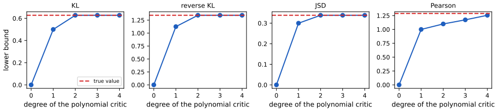
The bound can be far from the divergence. The inequality in (26.26) is exact only if \(\mathcal T\) contains \(t^*\). Take \(p^*=\N(0,1)\), \(q=\N(1.5,1.5^2)\) and polynomial critics of degree \(k\) (Figure x26.f). With the usual output activations (\(t=v\) for KL and Pearson, \(t=-e^v\) for reverse KL, \(t=\log2-\log(1+e^{-v})\) for the JSD row) the optimal pre-activation \(v^*\) is \(\log r\) (KL: \(t^*=1+\log r\); reverse KL: \(t^*=-q/p^*=-e^{-\log r}\); JSD: \(t^*=\log2-\log(1+1/r)\)), a quadratic in \(\bm x\) for two Gaussians. So a quadratic critic attains the exact divergence for those three, while for Pearson (\(t^*=2(r-1)\), not a polynomial) the bound climbs slowly with the degree. With a constant critic (degree 0) the bound is 0 for all four rows, and with linear critics it is 0.50, 1.13, 0.30 and 1.00 against true values 0.628, 1.345, 0.338 and 1.287. A sharper statement: if \(p^*=\N(0,1)\) and \(q=\N(0,s^2)\) are both even, the KL bound over linear critics equals 0 for every \(s\): the bound is concave in the critic parameters \((w,b)\) and even in \(w\), so its maximum is at \(w=0\), where it is \(\max_b\{b-e^{b-1}\}=0\). The generator therefore receives no signal from this restricted bound, although \(\Dkl(p^*\|q)=\log s+\frac1{2s^2}-\frac12\) changes with \(s\). This makes precise the book's remark that minimising a lower bound "provides no guarantees that the divergence will decrease".
26.2.4 Integral probability metrics
pp. 900–902 Instead of ratios one can compare distributions through differences. An integral probability metric (IPM) is \[ I_{\mathcal F}(p^*,q_{\bm\theta})=\sup_{f\in\mathcal F}\big|\E_{p^*}f(\bm x)-\E_{q_{\bm\theta}}f(\bm x)\big|, \tag{26.28} \] the largest gap in expectation over a class \(\mathcal F\) of witness (critic) functions. It is symmetric and satisfies the triangle inequality (it is a supremum of the absolute values of linear functionals of \(p^*-q\)), but it separates distributions only if \(\mathcal F\) is rich enough: for \(\mathcal F=\{0\}\) it is identically 0. The set of 1-Lipschitz functions gives the Wasserstein-1 distance, \[ W_1(p^*,q_{\bm\theta})=\sup_{\|f\|_{\Lip}\le1}\E_{p^*}f-\E_{q_{\bm\theta}}f\ \ge\ \max_{\bm\phi:\|D_{\bm\phi}\|_{\Lip}\le1}\E_{p^*}D_{\bm\phi}-\E_{q_{\bm\theta}}D_{\bm\phi}, \tag{26.29--26.31} \] with the critic regularised to be 1-Lipschitz (gradient penalty or spectral normalisation; gap 26.14), and the WassersteinGAN (Arjovsky et al., 2017) \[ \min_{\bm\theta}W_1\ge\min_{\bm\theta}\max_{\|D_{\bm\phi}\|_{\Lip}\le1}\E_{p^*}D_{\bm\phi}(\bm x)-\E_{q(\bm z)}D_{\bm\phi}(G_{\bm\theta}(\bm z)). \tag{26.32--26.33} \]
Filling the gap 26.5: Wasserstein critics: the easy direction, the one-dimensional critic, and what Figure 26.3(a) shows pp. 900–901, (26.29)–(26.33)
Proof
The full duality between the transport cost \(W_1=\inf_\pi\E_\pi\|X-Y\|\) and the supremum over 1-Lipschitz functions is proved in gap 6.25 (and in the deep-learning course, with the one-dimensional case); the book's (26.29) takes it as the definition. Three facts specific to this chapter:
(i) Easy direction. If \(\|f\|_{\Lip}\le1\) and \(\pi\) is any coupling of \(p^*\) and \(q\), then \(\E_{p^*}f-\E_qf=\E_\pi[f(X)-f(Y)]\le\E_\pi\|X-Y\|\); taking the infimum over \(\pi\) gives \(\sup_f\le W_1\). This is all that (26.31) needs: a regularised critic gives a lower bound, as in Section 26.2.3.
(ii) The optimal critic in one dimension. For distributions on \(\R\) with a finite first moment and a 1-Lipschitz \(f\), write \(f(x)=f(a)+\int_a^xf'(t)\d t\) with \(a\) below the support and use Fubini: \(\E_pf=f(a)+\int f'(t)\Pr_p(X>t)\d t\), so
\[ \E_pf-\E_qf=\int f'(t)\,\big(F_q(t)-F_p(t)\big)\d t\le\int|F_p-F_q|, \]
since \(|f'|\le1\); equality holds for \(f^*(x)=\int_{-\infty}^x\sgn\big(F_q(t)-F_p(t)\big)\d t\), which is 1-Lipschitz. Hence \(W_1=\int|F_p-F_q|\) and \(f^*\) is an optimal critic. (This agrees with a sample computation: scipy.stats.wasserstein_distance on 200 000 draws of a two-bump example gives 0.319 against 0.315 from the CDFs.)
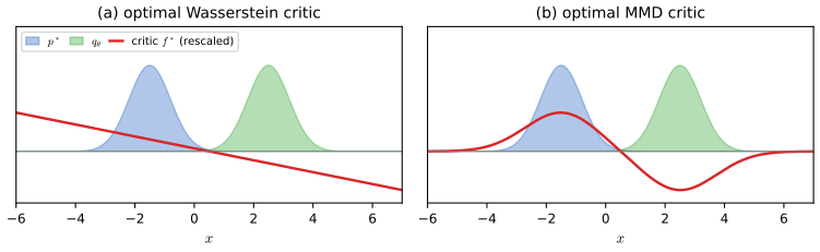
(iii) Figure 26.3(a). For two well separated bumps the model's distribution function lies below the data's everywhere, \(F_q\le F_p\), so \(\sgn(F_q-F_p)=-1\) everywhere and \(f^*(x)=-x+\text{const}\): the optimal critic is a straight line of slope \(-1\), which is the red line in the book's figure and in ours. The critic does not need to know where the bumps are, only which way mass has to move, and its gradient has unit size wherever the model samples lie, however far they are from the data.
If \(\mathcal F\) is the unit ball of the reproducing-kernel Hilbert space of a kernel \(\mathcal K\) (gap 18.11) the IPM is the maximum mean discrepancy, \[ \MMD(p^*,q_{\bm\theta})=\sup_{\|f\|_{\mathcal H}=1}\E_{p^*}f-\E_{q_{\bm\theta}}f,\tag{26.34} \] with the squared version, which needs only kernel evaluations at samples, \[ \MMD^2(p^*,q_{\bm\theta})=\E_{p^*(\bm x)}\E_{p^*(\bm x')}\mathcal K(\bm x,\bm x')-2\E_{p^*(\bm x)}\E_{q(\bm z)}\mathcal K(\bm x,G_{\bm\theta}(\bm z))+\E_{q(\bm z)}\E_{q(\bm z')}\mathcal K(G_{\bm\theta}(\bm z),G_{\bm\theta}(\bm z')). \tag{26.35--26.36} \] Minimising it directly, \(\min_{\bm\theta}\MMD^2\) (26.37), trains a generative matching network (Li et al., 2015; Dziugaite et al., 2015): there is no discriminator and no min-max game (Figure 26.1(b) was fitted this way, and the sixth variant of Figure x26.c). A fixed kernel can be poor for images; one can compose it with a learned feature map \(\bm\zeta_{\bm\phi}\) and maximise the squared MMD over \(\bm\phi\) so that the features are sensitive to the differences between \(p^*\) and \(q_{\bm\theta}\) (Li et al., 2017), which restores a min-max game, \[ \min_{\bm\theta}\max_{\bm\phi}\ \E\mathcal K(\bm\zeta_{\bm\phi}(\bm x),\bm\zeta_{\bm\phi}(\bm x'))-2\E\mathcal K(\bm\zeta_{\bm\phi}(\bm x),\bm\zeta_{\bm\phi}(\bm y))+\E\mathcal K(\bm\zeta_{\bm\phi}(\bm y),\bm\zeta_{\bm\phi}(\bm y')),\tag{26.38--26.39} \] with \(\bm\zeta_{\bm\phi}\) regularised to be injective. Unlike the Wasserstein distance and the \(f\)-divergences, (26.39) is estimated without a lower bound.
Filling the gap 26.6: MMD is a norm of mean embeddings; its estimators; learned features; and moment matching pp. 901–902, (26.34)–(26.40)
Proof
(26.34) and (26.35). Let \(\mathcal K\) be a positive-definite kernel with RKHS \(\mathcal H\) and feature map \(\varphi(\bm x)=\mathcal K(\bm x,\cdot)\), so \(f(\bm x)=\langle f,\varphi(\bm x)\rangle\) (reproducing property). If \(\E\sqrt{\mathcal K(\bm x,\bm x)}<\infty\) the mean embedding \(\mu_p=\E_p\varphi(\bm x)\in\mathcal H\) exists and \(\E_pf=\langle f,\mu_p\rangle\). Then \(\E_{p^*}f-\E_qf=\langle f,\mu_{p^*}-\mu_q\rangle\) and by Cauchy–Schwarz \(\sup_{\|f\|\le1}\langle f,\mu_{p^*}-\mu_q\rangle=\|\mu_{p^*}-\mu_q\|\), attained at the witness \(f^*=(\mu_{p^*}-\mu_q)/\|\mu_{p^*}-\mu_q\|\), \(f^*(\bm x)\propto\E_{p^*}\mathcal K(\bm x,\bm x')-\E_q\mathcal K(\bm x,\bm y)\) (Figure 26.3(b)). Expanding the squared norm, \(\|\mu_{p^*}-\mu_q\|^2=\langle\mu_{p^*},\mu_{p^*}\rangle-2\langle\mu_{p^*},\mu_q\rangle+\langle\mu_q,\mu_q\rangle\), and \(\langle\mu_p,\mu_q\rangle=\E_p\E_q\mathcal K(\bm x,\bm y)\): this is (26.35). If \(\mathcal K\) is characteristic (\(p\mapsto\mu_p\) injective; the Gaussian kernel is) then \(\MMD=0\) iff \(p^*=q\), so MMD is a metric. For two Gaussians and \(\mathcal K=\exp(-(x-y)^2/2\ell^2)\) the expectations are closed forms, \(\E\mathcal K(X,Y)=\sqrt{\ell^2/v}\,e^{-(m_1-m_2)^2/(2v)}\) with \(v=\ell^2+s_1^2+s_2^2\), which gives for \(\N(0,1)\) against \(\N(\delta,1)\) and \(\ell=1\): \(\MMD^2=\frac2{\sqrt3}(1-e^{-\delta^2/6})\). The grid quadrature used by the demonstration agrees with this to \(10^{-7}\).
Estimators. With samples \(\bm x_i\sim p^*\) (\(n\)) and \(\bm y_j\sim q\) (\(n'\)) the plug-in estimator \(\frac1{n^2}\sum_{i,i'}\mathcal K(\bm x_i,\bm x_{i'})-\frac2{nn'}\sum\mathcal K(\bm x_i,\bm y_j)+\frac1{n'^2}\sum\mathcal K(\bm y_j,\bm y_{j'})\) is the squared norm of the difference of empirical embeddings, hence \(\ge0\), but biased upwards (the diagonal terms \(\mathcal K(\bm x_i,\bm x_i)\) add \(\E\mathcal K(\bm x,\bm x)/n\)). Removing the diagonal terms (dividing by \(n(n-1)\) and \(n'(n'-1)\)) gives the unbiased U-statistic, which can be negative; under \(p^*=q\) it has mean 0 (confirmed by simulation: mean \(-0.0003\) against \(+0.021\) for the plug-in, with \(n=n'=40\)).
Learned features. If \(\bm\zeta\) is injective and \(\mathcal K\) characteristic, then \(p\mapsto\bm\zeta_\#p\) is injective and \(\bm\zeta_\#p\mapsto\mu\) is injective, so \(\mathcal K(\bm\zeta(\cdot),\bm\zeta(\cdot))\) is characteristic: this is the book's claim before (26.38). Without injectivity two distributions with the same image under \(\bm\zeta\) become indistinguishable, which is why the regulariser is needed.
Moment matching (Section 26.2.5). For statistics \(\bm s\), (26.40) minimises \(\|\E_{p^*}\bm s-\E_{q_{\bm\theta}}\bm s\|_2^2\). It is an IPM over the linear span of the components of \(\bm s\) and is a valid criterion only if \(\E_p\bm s=\E_q\bm s\Rightarrow p=q\). The choice \(\bm s(\bm x)=\bm x\) is not enough: \(\N(0,1)\) and \(\N(0,1.6^2)\) have the same mean and the RBF MMD2 between them is positive (\(>0.001\) at \(\ell=1\)). MMD is moment matching in a feature space: for \(\mathcal K(x,y)=(1+xy)^2=\langle(1,\sqrt2x,x^2),(1,\sqrt2y,y^2)\rangle\), \(\MMD^2=2(\E_pX-\E_qX)^2+(\E_pX^2-\E_qX^2)^2\) exactly (checked on 500 draws from two distributions), so the polynomial kernel of degree \(d\) matches the first \(d\) moments with binomial weights, while the Gaussian kernel has an infinite feature expansion and matches all of them. Ravuri et al. (2018) take \(\bm s_{\bm\phi}=[\nabla_{\bm\phi}D_{\bm\phi},h_1,\dots,h_n]\), the gradients of a trained classifier and its hidden activations; the gradients make the number of moments exceed the number of parameters, which is the condition for a consistent estimator of \(\bm\theta\).
26.2.5 Moment matching
p. 902 The method of moments (Pearson, 1936) minimises \(\|\E_{p^*}\bm s(\bm x)-\E_{q_{\bm\theta}}\bm s(\bm x)\|_2^2\) (26.40). The statistic matters: \(\bm s(\bm x)=\bm x\) matches only the mean, the score \(\nabla_{\bm x}\log q_{\bm\theta}\) gives a consistent estimator but needs the density, and MMD is moment matching in an RKHS feature space (gap 26.6, which covers this subsection).
26.2.6 On density ratios and differences
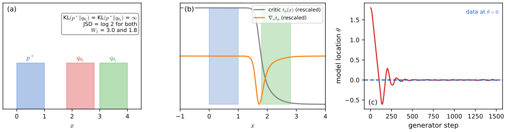
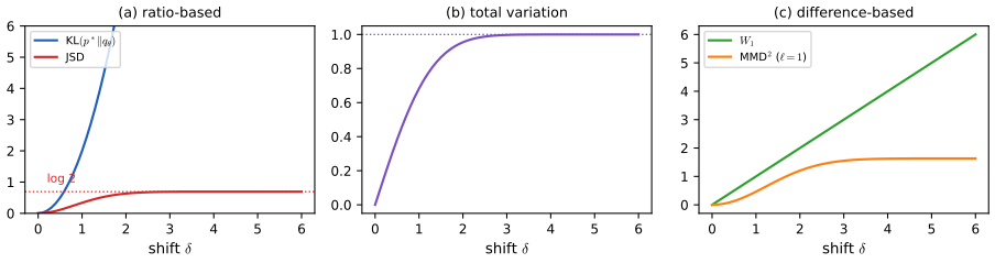
pp. 902–904 A much-quoted weakness of ratio-based criteria is that they cannot compare distributions with disjoint supports: where \(p^*>0=q_{\bm\theta}\) the ratio is infinite and where \(q_{\bm\theta}>0=p^*\) it is 0, so \(\Dkl(p^*\|q_{\bm\theta})=\infty\) and \(\JSD=\log2\) whatever \(\bm\theta\) is (Figure 26.4(a): \(\Dkl(p^*\|q_{\bm\theta_1})=\Dkl(p^*\|q_{\bm\theta_2})=\infty\) although \(q_{\bm\theta_2}\) is closer). The difference-based Wasserstein distance and MMD constrain the critic's smoothness and give a signal (Figure 26.3). In practice, however, the critic of an \(f\)-divergence or of a classifier is a smooth network that approximates the sharp ratio, and its input gradient tells the generator where the data are (Figure 26.4(b)); this lets the generator learn from any initialisation (Fedus et al., 2018), so the distinction is "less significant in practice". The book closes with the caveat of gap 26.4: the generator minimises a lower bound, which need not decrease with the divergence, unlike the upper bound of the VAE.
Filling the gap 26.7: disjoint supports: what is constant and what is not, and the smooth critic of Figure 26.4(b) pp. 902–904, Figure 26.4
Proof
The ratio-based criteria are constant. If \(p\perp q\) (disjoint supports): \(\Dkl(p\|q)=\int p\log\frac pq=\infty\) because \(q=0\) on a set of positive \(p\)-measure; \(\TV(p,q)=1\) since \(\int\min(p,q)=0\); \(\JSD=\log2\) by the equality case of gap 26.2 (equivalently \(m=p/2\) on the support of \(p\), so \(\Dkl(p\|m)=\log2\), and likewise for \(q\)); every \(f\)-divergence equals the constant \(f(0)+\lim_{u\to\infty}f(u)/u\) (\(\infty\) for KL, \(2\log2\) for the JSD row). None depends on \(\bm\theta\) while the supports stay disjoint, so the gradient with respect to \(\bm\theta\) is zero almost everywhere.
The difference-based criteria vary. Take \(p^*=\mathcal U(0,1)\) and \(q_\theta=\mathcal U(\theta,\theta+1)\), \(\theta\ge1\). The distribution functions differ by \(F_p(x)-F_q(x)\), which is a trapezoid of height 1 and area \(\theta\), so \(W_1=\int|F_p-F_q|=\theta\) (a translation by \(\theta\) costs exactly \(\theta\)); \(\MMD^2\) with a bounded characteristic kernel depends on \(\theta\) through \(\E\mathcal K(X,Y)\) and tends to a constant only when the kernel can no longer see the gap (Figure x26.a(c)). In the two-uniform example of Figure 26.4 the values are \(W_1=3.0\) and \(1.8\) for \(\theta_1=3\) and \(\theta_2=1.8\), so \(q_{\theta_2}\) is the closer model, which no ratio-based quantity can say.
The learned critic of Figure 26.4(b,c). Train \(t_{\bm\phi}\), a small tanh network, on the KL bound \(\E_{p^*}t-\E_{q_\theta}e^{t-1}\) (the KL row of Table 26.2) with \(p^*=\mathcal U(0,1)\) and \(q_\theta=\mathcal U(1.8,2.8)\). At the optimum of the unrestricted problem \(t^*=1+\log r\) is \(+\infty\) on the data and \(-\infty\) on the model; the network instead learns a smooth sigmoid-like step (panel (b)) whose gradient points from the model to the data. Using it, the generator moves its location by descending \(-\E_{q_\theta}e^{t_{\bm\phi}(\theta+z)-1}\), the \(\theta\)-dependent part of the bound, re-fitting the critic three times per step: \(\theta\) travels from 1.8 to the data location 0 in about 100 steps, overshoots to about \(-0.6\) and back to \(0.3\) while the critic adapts, and stays within 0.05 of 0 after 300 steps (panel (c)), although the true divergence is \(\infty\) all along until the supports touch. This is the book's point: a smooth critic provides the "gradient signal on how to move distribution mass". The price is the one of gap 26.4: the objective being descended is a bound, and with a more restricted critic family it can be flat.
26.3 Generative adversarial networks
p. 904 The learning principles specify criteria; to turn them into an algorithm one needs loss functions (26.3.1), a way to descend them (26.3.2), an understanding of what goes wrong (26.3.3), improvements (26.3.4) and a notion of convergence (26.3.5).
26.3.1 From learning principles to loss functions
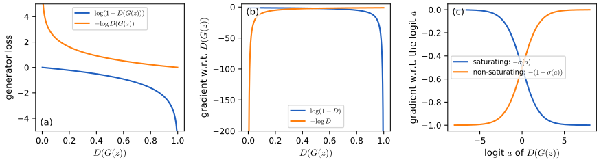
pp. 904–905 Most criteria of Section 26.2 give a zero-sum game: the critic maximises the quantity that the generator minimises, \[ \min_{\bm\theta}\max_{\bm\phi}V(\bm\phi,\bm\theta),\qquad V(\bm\phi,\bm\theta)=\tfrac12\E_{p^*}[\log D_{\bm\phi}(\bm x)]+\tfrac12\E_{q_{\bm\theta}}[\log(1-D_{\bm\phi}(\bm x))]\ \text{(the original GAN)}. \tag{26.41--26.42} \] The structure need not be zero-sum. For the generator, minimising \(\E_{q_{\bm\theta}}\log(1-D_{\bm\phi})\) says "make the discriminator call my samples fake less often"; an equally natural goal is to maximise the probability of being called real, i.e. minimise \(\E_{q_{\bm\theta}}[-\log D_{\bm\phi}]\), the non-saturating loss (Goodfellow et al., 2014). Its gradient is strong exactly when the discriminator confidently rejects the generator's samples, \(D(G(z))\) small (Figure 26.5; gap 26.8). Other non-zero-sum GANs include LS-GAN, hinge-loss GANs and relativistic GANs. In general, \[ \min_{\bm\phi}L_D(\bm\phi,\bm\theta);\qquad\min_{\bm\theta}L_G(\bm\phi,\bm\theta), \tag{26.43} \] zero-sum when \(-L_D=L_G=V\), and most losses have the form \[ L_D=\E_{p^*}g(D_{\bm\phi}(\bm x))+\E_{q(\bm z)}h(D_{\bm\phi}(G_{\bm\theta}(\bm z))),\qquad L_G=\E_{q(\bm z)}l(D_{\bm\phi}(G_{\bm\theta}(\bm z))), \tag{26.44--26.45} \] with \(g,h,l:\R\to\R\): the original GAN has \(g(t)=-\log t\), \(h(t)=-\log(1-t)\), \(l(t)=\log(1-t)\); the non-saturating GAN the same \(g,h\) and \(l(t)=-\log t\). (For the Wasserstein and \(f\)-GAN rows of the book's list the signs are those of the objective to be maximised by the critic, not of a loss to be minimised as in (26.43); see Notes on the book.)
Filling the gap 26.8: saturating and non-saturating gradients, and what each descends when the discriminator is optimal pp. 905–906, Figure 26.5
Proof
Vanishing gradients (Figure 26.5). As functions of \(D=D(G(z))\) the two generator losses have derivatives \(\frac{\d}{\d D}\log(1-D)=-\frac1{1-D}\) and \(\frac{\d}{\d D}(-\log D)=-\frac1D\) (Figure 26.5(b)): the non-saturating loss has the large gradient when \(D\to0\), the saturating one when \(D\to1\). The gradient the generator uses passes through the discriminator's logit \(a\), \(D=\sigma(a)\), where \(\sigma'(a)=D(1-D)\) multiplies both: \(\frac{\d}{\d a}\log(1-\sigma(a))=-\sigma(a)\to0\) as \(a\to-\infty\), while \(\frac{\d}{\d a}[-\log\sigma(a)]=-(1-\sigma(a))\to-1\) (Figure 26.5(c), not in the book). So a saturating generator facing a confident discriminator (\(a\ll0\)) gets a gradient of size \(\sigma(a)\approx0\); a non-saturating one keeps size \(\approx1\).
What each loss descends against \(D^*\). Fix the current parameter \(\bm\theta_0\), let \(D^*=p/(p+q_0)\) with \(q_0=q_{\bm\theta_0}\), and write \(q=q_{\bm\theta}\). For a function \(h\) that does not depend on \(\bm\theta\), \(\nabla_{\bm\theta}\int q\,h=\int(\nabla_{\bm\theta}q)\,h\), and \(\int\nabla_{\bm\theta}q=0\). The gradient of the generator loss with \(D^*\) held fixed (which is what a generator step with an optimal discriminator uses) is therefore, at \(\bm\theta_0\), \[ \nabla_{\bm\theta}\tfrac12\E_q\log(1-D^*)=\tfrac12\int\nabla q\,\log\frac{q_0}{p+q_0},\qquad\nabla_{\bm\theta}\E_q[-\log D^*]=\int\nabla q\,\log\frac{p+q_0}{p}. \] On the other side, differentiate the divergences themselves (all with the true dependence of \(m=\frac{p+q}2\) on \(\bm\theta\)): \(\nabla\Dkl(p\|m)=-\int p\frac{\nabla q}{p+q}\) and \(\nabla\Dkl(q\|m)=\int\nabla q\log\frac qm+\int\nabla q-\int q\frac{\nabla q}{p+q}\), whose sum is \(\int\nabla q\log\frac qm\) (the terms \(-\int\frac{(p+q)\nabla q}{p+q}+\int\nabla q\) cancel). So \(\nabla(2\JSD)=\int\nabla q\log\frac{2q}{p+q}\) and, with \(\int\nabla q=0\), \[ \boxed{\ \nabla_{\bm\theta}\tfrac12\E_q\log(1-D^*)\big|_{D^*\text{ fixed}}=\nabla_{\bm\theta}\JSD(p,q_{\bm\theta})\ } \] \[ \boxed{\ \nabla_{\bm\theta}\E_q[-\log D^*]\big|_{D^*\text{ fixed}}=\nabla_{\bm\theta}\big[\Dkl(q_{\bm\theta}\|p)-2\JSD(p,q_{\bm\theta})\big]\ } \] The second holds because \(\nabla\Dkl(q\|p)=\int\nabla q\log\frac qp\) and \(\log\frac qp-\log\frac{2q}{p+q}=\log\frac{p+q}{2p}\), which differs from \(\log\frac{p+q}p\) by a constant (killed by \(\int\nabla q=0\)). The first identity is the envelope theorem and shows that the saturating GAN with an optimal discriminator descends the JSD exactly. The second is the result of Arjovsky and Bottou (2017): the non-saturating GAN descends the reverse KL minus twice the JSD. The reverse KL \(\Dkl(q\|p)\) is mode seeking and heavily penalises samples where \(p\) is small; the term \(-2\JSD\) pushes \(q\) away from \(p\). The two cancel in a way that gives a useful gradient early on (where JSD saturates and its gradient vanishes) but is not the gradient of a divergence. Numerical example (finite differences on a grid, \(p=\N(0.3,1)\), \(q=\N(\mu,\sigma^2)\) at \((\mu,\sigma)=(1.2,0.8)\)): the saturating fixed-\(D^*\) gradient is \((0.2127,-0.1756)\), equal to \(\nabla\JSD\); the non-saturating one is \((0.4745,-0.0989)\), equal to \(\nabla[\Dkl(q\|p)-2\JSD]\). Moreover \(\E_q[-\log D^*]=\log2+\Dkl(q\|p)-\Dkl(q\|m)\) (the value, not the gradient), as one checks by writing \(-\log D^*=\log2+\log\frac mp\).
26.3.2 Gradient descent
pp. 905–907 Solving the inner problem fully for each generator update is too expensive, so one alternates a few discriminator steps with a generator step, each treating the other player's parameters as fixed:
Algorithm 26.1: general GAN training with alternating updates
- Initialise \(\bm\phi,\bm\theta\).
- For each training iteration: for \(K\) steps, update \(\bm\phi\) with the gradient \(\nabla_{\bm\phi}L_D(\bm\phi,\bm\theta)\); then update \(\bm\theta\) with \(\nabla_{\bm\theta}L_G(\bm\phi,\bm\theta)\).
- Return \(\bm\phi,\bm\theta\).
The discriminator gradient moves under the expectation because \(p^*\) and \(q(\bm z)\) do not depend on \(\bm\phi\): \[ \nabla_{\bm\phi}L_D=\E_{p^*}\nabla_{\bm\phi}g(D_{\bm\phi}(\bm x))+\E_{q_{\bm\theta}}\nabla_{\bm\phi}h(D_{\bm\phi}(\bm x)), \tag{26.46--26.47} \] computed by back-propagation and estimated by minibatch Monte Carlo. For the generator, the distribution under the expectation depends on \(\bm\theta\), so the order of derivative and integral cannot be swapped in \(\nabla_{\bm\theta}\E_{q_{\bm\theta}(\bm x)}l(D_{\bm\phi}(\bm x))\) (26.48); but writing the expectation over the fixed \(q(\bm z)\) (the reparameterisation trick, Section 6.3.5) it can: \[ \nabla_{\bm\theta}L_G=\nabla_{\bm\theta}\E_{q(\bm z)}l(D_{\bm\phi}(G_{\bm\theta}(\bm z)))=\E_{q(\bm z)}\nabla_{\bm\theta}\,l(D_{\bm\phi}(G_{\bm\theta}(\bm z))). \tag{26.49} \] This gives the training algorithm used in practice:
Algorithm 26.2: GAN training
- Initialise \(\bm\phi,\bm\theta\).
- For each training iteration: for \(K\) steps, sample a minibatch \(\bm z_1,\dots,\bm z_M\sim q(\bm z)\) and \(\bm x_1,\dots,\bm x_M\sim p^*\); update the discriminator by stochastic gradient descent with \(\nabla_{\bm\phi}\frac1M\sum_m[g(D_{\bm\phi}(\bm x_m))+h(D_{\bm\phi}(G_{\bm\theta}(\bm z_m)))]\).
- Sample a fresh minibatch \(\bm z_m\sim q(\bm z)\); update the generator with \(\nabla_{\bm\theta}\frac1M\sum_ml(D_{\bm\phi}(G_{\bm\theta}(\bm z_m)))\).
- Return \(\bm\phi,\bm\theta\).
The code implements exactly this (train_gan in ch26_gans.py) and every experiment below uses it.
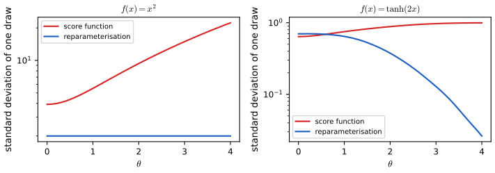
Filling the gap 26.9: why (26.49) is legitimate, what the score-function alternative costs, and the variances pp. 906–907, (26.46)–(26.49); Section 26.7.4
Proof
(26.47) and (26.49). Both are differentiation under the integral sign. For (26.47) the integrand \(g(D_{\bm\phi}(\bm x))p^*(\bm x)\) is differentiable in \(\bm\phi\) and has an integrable \(\bm\phi\)-derivative bound locally (dominated convergence), so the derivative can be taken inside. For (26.49), \(l(D_{\bm\phi}(G_{\bm\theta}(\bm z)))\) is differentiable in \(\bm\theta\) for each \(\bm z\) (the generator is a differentiable network), \(q(\bm z)\) is independent of \(\bm\theta\), and again dominated convergence lets \(\nabla_{\bm\theta}\) move inside. In (26.48), by contrast, the integral is over \(\bm x\) against a density \(q_{\bm\theta}(\bm x)\) that depends on \(\bm\theta\) and, by gap 26.1, may not exist: there the derivative of the integral is not the integral of the derivative.
The score-function estimator. If \(q_{\bm\theta}\) does have a density, \(\nabla_{\bm\theta}\E_{q_{\bm\theta}}f=\E_{q_{\bm\theta}}[f(\bm x)\nabla_{\bm\theta}\log q_{\bm\theta}(\bm x)]\) (gap 6.3), also an unbiased estimator, and the only one available when \(\bm x\) is discrete (so that no differentiable \(G_{\bm\theta}\) maps noise to data), e.g. text (Section 26.7.4). Its variance is typically far larger. A closed form: \(x\sim\N(\theta,1)\) and \(f(x)=x^2\), so \(\frac{\d}{\d\theta}\E f=2\theta\). Write \(x=\theta+\varepsilon\). The reparameterised single-draw estimator is \(2(\theta+\varepsilon)\) with variance \(4\). The score-function estimator is \(f(x)\,(x-\theta)=(\theta+\varepsilon)^2\varepsilon\) with mean \(2\theta\) (since \(\E\varepsilon^3=0\), \(\E\varepsilon^2=1\)) and second moment \(\E[(\theta+\varepsilon)^4\varepsilon^2]=\theta^4\E\varepsilon^2+6\theta^2\E\varepsilon^4+\E\varepsilon^6=\theta^4+18\theta^2+15\), so \[ \var=\theta^4+14\theta^2+15\quad(\text{against }4\text{ for the reparameterised estimator}),\] a ratio of standard deviations of \(1.9\) at \(\theta=0\) and \(11\) at \(\theta=4\) (Figure x26.e; simulation: standard deviations 3.88, 5.49, 9.34, 22.3 at \(\theta=0,1,2,4\)). More general statements are in gap 6.4. Because the variance of the score-function estimator grows with the size of \(f\), methods for text GANs either pre-train by maximum likelihood and fine-tune with small steps or avoid the estimator by continuous relaxations (Section 26.7.4).
26.3.3 Challenges with GAN training
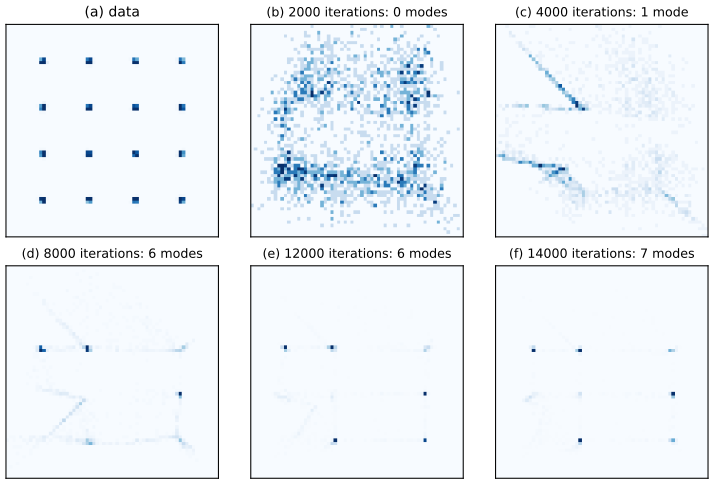
p. 907 The adversarial game is hard to analyse and to stabilise. Mode collapse is the failure of the generator to cover all modes of the data distribution: it converges to a distribution that covers a few peaks only. Mode hopping is the related cat-and-mouse behaviour: once the generator is good at one mode it produces more of it; if the discriminator cannot tell real from fake there the generator has no incentive to expand its support, but if the discriminator eventually learns to, the generator can "hop" to another mode. Large batches, a stronger discriminator, regularisation of both players and better optimisers make both rarer.
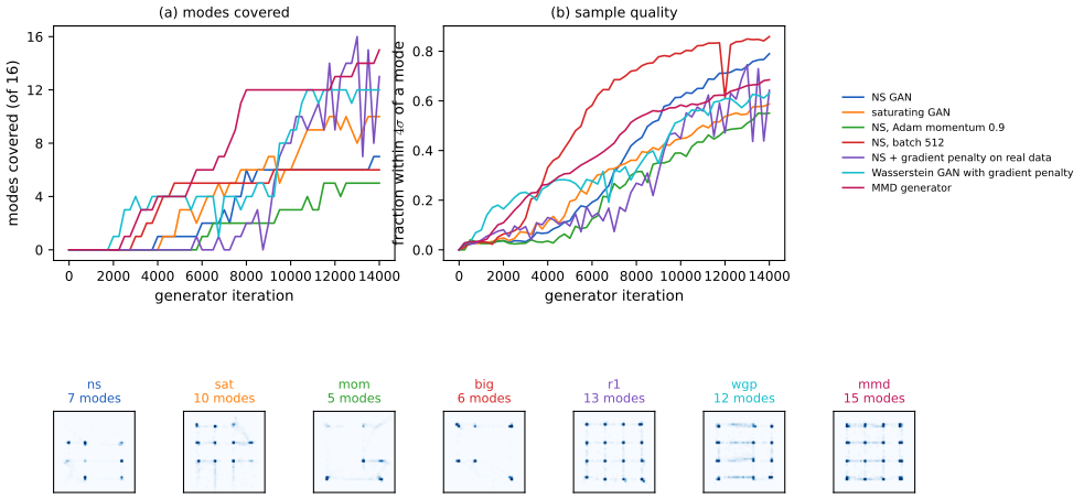
Figure 26.6 trains the plain algorithm (Algorithm 26.2 with \(K=1\), the non-saturating loss) on a mixture of 16 equally weighted Gaussians on a \(4\times4\) grid. Our version has component standard deviation 0.05 (grid spacing 2), generator and discriminator with two hidden layers of 32 ReLU units, a two-dimensional latent code, Adam with learning rate \(10^{-3}\) and momentum 0.5, and minibatches of 64; 14 000 iterations take about 30 s. A mode is counted as covered when at least half its fair share of the generated samples (1/32) lies within four standard deviations of it. After 2000 iterations no mode is covered, after 4000 one, after 8000, 12 000 and 14 000 iterations 6, 6 and 7 of the 16 (the fraction of samples close to some mode is 0.04, 0.07, 0.44, 0.71 and 0.79): the covered set grows from \(\{6\}\) to \(\{2,6\}\), to six modes and finally seven (modes are numbered row by row), and the other nine are never found within the budget: partial mode collapse. The hopping described by the book, where covered modes are abandoned again, shows up in other variants (the number of modes covered by the R1 and Wasserstein runs of Figure x26.c goes down as well as up).
26.3.4 Improving GAN optimization
p. 908 Hyperparameters such as momentum are crucial: lower momentum than in supervised learning is preferred, and Adam (Kingma and Ba, 2015) gives a large boost (Radford et al., 2016). Other optimisers reduce variance (Chavdarov et al., 2019), back-propagate through gradient steps so that the generator is good against the updated discriminator (Metz et al., 2017), or use a local bilinear approximation of the game (Schaefer and Anandkumar, 2019); they cost more and scale less well. Figure x26.c compares seven variants of the baseline on the sixteen-mode problem, all with the same initialisation and 14 000 iterations (one seed each, so the ranking is only an illustration):
| variant | modes covered at 14 000 | fraction within \(4\sigma\) |
|---|---|---|
| non-saturating (baseline) | 7 | 0.79 |
| saturating loss | 10 | 0.59 |
| Adam momentum 0.9 (baseline 0.5) | 5 | 0.55 |
| batch 512 (baseline 64) | 6 | 0.86 |
| R1 gradient penalty on real data, \(\gamma=10\) | 13 | 0.64 |
| Wasserstein GAN with gradient penalty (weight 1, 5 critic steps) | 12 | 0.63 |
| MMD generator (no discriminator, batch 256) | 15 | 0.69 |
In this run lower momentum does better than higher, as the book recommends; larger batches give sharper samples but did not cover more modes here; the gradient penalty (which also appears in the stability analysis of gap 26.11) and the Wasserstein critic recover most modes, and the discriminator-free MMD generator the most. The Wasserstein variant needed a penalty weight of 1 and five critic steps to be competitive in this short budget (weight 10 with learning rate \(10^{-3}\) covered only 4 modes, and with smaller learning rates fewer still within 14 000 steps), so it is also the most expensive.
26.3.5 Convergence of GAN training
pp. 908–912 If the discriminator is optimal the generator minimises a divergence, so with infinite capacity and perfect optimisation it learns the data distribution (Section 26.2); in game-theoretic terms this proves the existence of a global Nash equilibrium, a point at which neither player can gain by changing its parameters alone: for the original GAN \(q_{\bm\theta}=p^*\) and \(D_{\bm\phi}=\frac{p^*}{p^*+q_{\bm\theta}}=\tfrac12\). These guarantees assume infinite capacity and ignore the trajectory. In practice the losses are not decreased at every step (Fedus et al., 2018) and one studies local equilibria: a stationary point (\(\nabla_{\bm\phi}L_D=0\), \(\nabla_{\bm\theta}L_G=0\)) at which each player's Hessian (\(\nabla^2_{\bm\phi}L_D\), \(\nabla^2_{\bm\theta}L_G\)) is positive semi-definite (Ratliff et al., 2016); a local Nash equilibrium need not exist (Farnia and Ozdaglar, 2020) and weaker notions are used. Gap 26.11 sets out the global statement precisely: at \(D=\frac12\) every generator is a best response, so \(q=p^*\) is a Nash equilibrium but not a strict one.
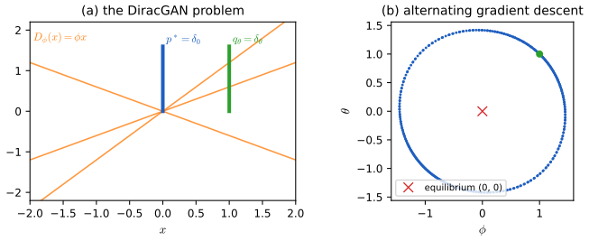
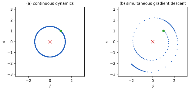
The DiracGAN (Mescheder et al., 2018) shows why convergence analysis matters. The data distribution is a point mass at 0, the generator a point mass at \(\theta\), \(G_\theta(z)=\theta\), and the discriminator is linear, \(D_\phi(x)=\phi x\). With a zero-sum game \(g=h=-l\), \[ L_D=\E_{p^*}[-l(D_\phi(x))]+\E_{q_\theta}[-l(D_\phi(x))]=-l(0)-l(\theta\phi),\qquad L_G=l(0)+l(\theta\phi), \tag{26.50--26.51} \] where \(l\) depends on the GAN (e.g. \(l(z)=-\log(1+e^{-z})\)); the unique equilibrium is \(\theta=\phi=0\). Under alternating gradient descent (Algorithm 26.1) the iterates do not converge but circle the equilibrium (Figure 26.7). Two theoretical approaches analyse the dynamics: the discrete updates with learning rates \(\alpha_h,\lambda_h\), \[ \bm\phi_t=\bm\phi_{t-1}-\alpha_h\nabla_{\bm\phi}L_D(\bm\phi_{t-1},\bm\theta_{t-1}),\quad\bm\theta_t=\bm\theta_{t-1}-\lambda_h\nabla_{\bm\theta}L_G(\bm\phi_t,\bm\theta_{t-1})\quad\text{(alternating)}, \tag{26.52--26.53} \] \[ \bm\phi_t=\bm\phi_{t-1}-\alpha_h\nabla_{\bm\phi}L_D(\bm\phi_{t-1},\bm\theta_{t-1}),\quad\bm\theta_t=\bm\theta_{t-1}-\lambda_h\nabla_{\bm\theta}L_G(\bm\phi_{t-1},\bm\theta_{t-1})\quad\text{(simultaneous)}, \tag{26.54--26.55} \] and the underlying continuous dynamics, of which the updates are Euler discretisations, \[ \dot{\bm\phi}=-\nabla_{\bm\phi}L_D(\bm\phi,\bm\theta),\qquad\dot{\bm\theta}=-\nabla_{\bm\theta}L_G(\bm\phi,\bm\theta). \tag{26.56--26.57} \] Stability analysis looks at the eigenvalues of the Jacobian of the game at a stationary point, \[ J=\begin{pmatrix}-\nabla_{\bm\phi}\nabla_{\bm\phi}L_D&-\nabla_{\bm\theta}\nabla_{\bm\phi}L_D\\-\nabla_{\bm\phi}\nabla_{\bm\theta}L_G&-\nabla_{\bm\theta}\nabla_{\bm\theta}L_G\end{pmatrix}: \tag{26.58} \] all real parts negative means asymptotic stability, a positive real part means instability. For the DiracGAN, at \(\theta=\phi=0\), \[ J=\begin{pmatrix}0&l'(0)\\-l'(0)&0\end{pmatrix},\qquad\lambda_\pm=\pm i\,l'(0), \tag{26.59} \] so the real parts vanish and there is no asymptotic convergence; here one sees that convergence indeed fails because \(\theta^2+\phi^2\) is conserved by the flow, \(\frac{\d}{\d t}(\theta^2+\phi^2)=-2\theta\phi\,l'(\theta\phi)+2\phi\theta\,l'(\theta\phi)=0\) (Figure 26.8, left). Explicit regularisation helps convergence (Nagarajan and Kolter, 2017; Balduzzi et al., 2018); under conditions, simultaneous updates reach a local Nash equilibrium (Mescheder et al., 2017), and the results depend on the learning rate. The two approaches can disagree: simultaneous updates spiral outwards (Figure 26.8, right) although the continuous flow keeps a fixed radius, because the discretisation error matters (Rosca et al., 2021), which motivates higher-order integrators such as RungeKutta4 (Qin et al., 2020). Finally, convergence to an equilibrium does not mean the distribution has been learned well: the loss landscape can have equilibria that do not capture the data, so convergence analysis must be complemented by an analysis of what gradient-based learning in the game does to the learned distribution.
Filling the gap 26.10: DiracGAN in full: the conserved radius, the exact radius law of simultaneous updates and the invariant ellipse of alternating updates pp. 909–912, (26.50)–(26.59), Figures 26.7–26.8
Proof
Write \(c(\theta\phi)=l'(\theta\phi)\) and \(c_0=l'(0)\). From (26.50)–(26.51), \(\nabla_\phi L_D=-\theta c(\theta\phi)\) and \(\nabla_\theta L_G=\phi c(\theta\phi)\). The flow (26.56)–(26.57) is \[ \dot\phi=\theta\,c(\theta\phi),\qquad\dot\theta=-\phi\,c(\theta\phi). \] Equilibrium and Jacobian. For a strictly monotone \(l\) with \(c>0\) everywhere (logistic: \(c(z)=\sigma(-z)\)) the field vanishes iff \(\theta=\phi=0\). Differentiating at the origin, where \(\partial_\phi(\theta c)=\theta^2c'\to0\) and \(\partial_\theta(\theta c)=c+\theta\phi c'\to c_0\): \(J=\begin{pmatrix}0&c_0\\-c_0&0\end{pmatrix}\), with \(\det(J-\lambda I)=\lambda^2+c_0^2\), so \(\lambda=\pm ic_0\), (26.59). For the logistic \(l\), \(c_0=\tfrac12\); for \(l(z)=z\), \(c_0=1\).
Conservation. \(\frac{\d}{\d t}(\theta^2+\phi^2)=2\theta\dot\theta+2\phi\dot\phi=-2\theta\phi c+2\phi\theta c=0\) for any \(l\): the exact flow moves on circles. A fourth-order Runge–Kutta integration with step 0.01 keeps the radius to within \(10^{-9}\) over 60 time units, so the "continuous" panel of Figure 26.8 is circular.
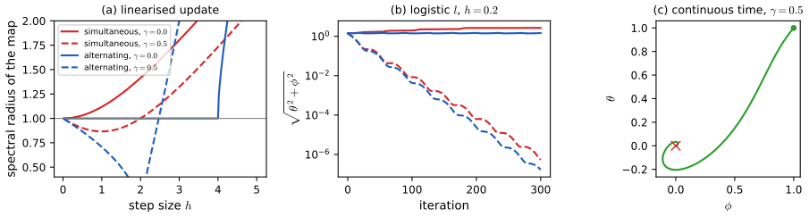
Simultaneous updates: an exact law. (26.54)–(26.55) give \(\phi'=\phi+h\theta c\), \(\theta'=\theta-h\phi c\) with \(c=c(\theta\phi)\). Then \(\phi'^2+\theta'^2=\phi^2+\theta^2+2h\theta\phi c-2h\theta\phi c+h^2c^2(\theta^2+\phi^2)\), i.e. \[ r_{t+1}^2=r_t^2\big(1+h^2c(\theta_t\phi_t)^2\big),\qquad r^2=\theta^2+\phi^2. \] The radius never decreases and grows strictly whenever \(c\ne0\): at the equilibrium's linearisation by the factor \(\sqrt{1+h^2c_0^2}\) per step (the spectral radius of \(I+hJ\)). For the logistic \(l\) the factor is \(\sqrt{1+h^2\sigma(-\theta\phi)^2}\), which decays as \(|\theta\phi|\) grows, so the spiral slows down: from \((1,1)\) with \(h=0.3\) the radius after 150 steps is 2.86 (Figure 26.8, right; Figure x26.b(b) shows that it levels off). For the bilinear game \(l(z)=z\) the factor \(\sqrt{1+h^2}\) is constant and the radius diverges geometrically.
Alternating updates: a closed orbit. (26.52)–(26.53) with \(\alpha_h=\lambda_h=h\): \(\phi'=\phi+h\theta c(\theta\phi)\), then \(\theta'=\theta-h\phi'c(\theta\phi')\). Near the equilibrium \(c\approx c_0\); with \(\kappa=hc_0\), \[ \begin{pmatrix}\phi'\\\theta'\end{pmatrix}=\begin{pmatrix}1&\kappa\\-\kappa&1-\kappa^2\end{pmatrix}\begin{pmatrix}\phi\\\theta\end{pmatrix}=:M\begin{pmatrix}\phi\\\theta\end{pmatrix},\qquad\det M=1,\quad\operatorname{tr}M=2-\kappa^2. \] The eigenvalues are of modulus 1 (a rotation) iff \(|\operatorname{tr}M|<2\), i.e. \(0<\kappa<2\), \(h<2/c_0\); for \(\kappa>2\) the trace is below \(-2\), one eigenvalue has modulus above 1, and the iterates diverge. For \(\kappa<2\) a direct expansion shows that \(Q(\phi,\theta)=\phi^2+\theta^2+\kappa\,\phi\theta\) is invariant: \(Q(\phi',\theta')=Q(\phi,\theta)\) (the coefficients of \(\phi^2\), \(\phi\theta\), \(\theta^2\) are \(1+\kappa^2-\kappa^2\), \(2\kappa-2\kappa(1-\kappa^2)+\kappa(1-2\kappa^2)=\kappa\) and \(\kappa^2+(1-\kappa^2)^2+\kappa^2(1-\kappa^2)=1\)). \(Q\) is positive definite for \(\kappa<2\), so the orbits are closed ellipses around the equilibrium with rotation angle \(\omega\), \(\cos\omega=1-\kappa^2/2\): for the logistic \(l\) and \(h=0.2\), \(\kappa=0.1\), \(\omega=0.1000\) rad, a period of 62.8 steps. The orbit never approaches the equilibrium and never leaves it: this is the circle of Figure 26.7. In the nonlinear logistic game the radius wobbles between 1.41 and 1.49 over 400 iterations from \((1,1)\) (the nonlinearity perturbs the invariant ellipse but does not break it). With \(h=4.4\) (\(\kappa=2.2\)) the spectral radius is 2.43 and the iterates blow up (demonstration, preset 5).
Why the two disagree. The continuous flow and alternating updates conserve a (slightly different) quadratic form; simultaneous updates add \(h^2c^2r^2\) to the squared radius at every step. The gap is a discretisation error of order \(h\) in the radius per unit time: simultaneous gradient descent is the explicit Euler scheme, which for a pure rotation is unstable for every step size, whereas the alternating scheme is the symplectic (semi-implicit) Euler scheme, which preserves the area and a modified energy.
Filling the gap 26.11: stability, the gradient penalty, and the Nash equilibrium of the original game pp. 908–912, Section 26.3.5
Proof
Stability from the Jacobian. If all eigenvalues of \(J\) at a stationary point have negative real parts, the stationary point is locally asymptotically stable for the flow (26.56)–(26.57) (Lyapunov's indirect method); a positive real part makes it unstable; if the real parts are zero the linearisation is inconclusive, which is why the DiracGAN needs the exact conservation law of gap 26.10. For the discrete updates the analogue is the spectral radius of the Jacobian of the update map: below 1 for local convergence, above 1 for divergence.
A gradient penalty. Penalising the discriminator's gradient at the data (the R1 penalty of Mescheder et al., 2018), \(\tfrac\gamma2\E_{p^*}\|\nabla_{\bm x}D_{\bm\phi}\|^2\), adds \(\tfrac\gamma2\phi^2\) to \(L_D\) in the DiracGAN since \(\nabla_xD_\phi=\phi\). The flow becomes \(\dot\phi=\theta c-\gamma\phi\), \(\dot\theta=-\phi c\) and \[ J=\begin{pmatrix}-\gamma&c_0\\-c_0&0\end{pmatrix},\qquad\lambda^2+\gamma\lambda+c_0^2=0,\qquad\lambda=-\tfrac\gamma2\pm\sqrt{\tfrac{\gamma^2}4-c_0^2}. \] For \(\gamma>0\) both roots have negative real part (their sum is \(-\gamma\) and product \(c_0^2>0\)), so the equilibrium is asymptotically stable; for \(\gamma<2c_0\) the roots are complex with real part exactly \(-\gamma/2\): the radius decays like \(e^{-\gamma t/2}\) (simulation of the \(l(z)=z\) game, \(c_0=1\), \(\gamma=0.5\): fitted decay rate \(-0.2500\)). In the discrete simultaneous scheme the map \(I+hJ\) has eigenvalues \(1+h\lambda\), with \[ |1+h\lambda|^2=\big(1-\tfrac{h\gamma}2\big)^2+h^2\big(c_0^2-\tfrac{\gamma^2}4\big)=1-h\gamma+h^2c_0^2\quad(\gamma<2c_0), \] which is below 1 iff \(h<\gamma/c_0^2\). With \(c_0=\tfrac12\), \(\gamma=0.5\) the condition is \(h<2\) and at \(h=0.2\) the spectral radius is \(\sqrt{0.91}=0.9539\), so the same simultaneous update that spirals out for \(\gamma=0\) (spectral radius \(\sqrt{1+0.01}=1.005\)) now contracts (Figure x26.b; demonstration, preset 4). The alternating update with the same penalty has spectral radius 0.9487 at \(h=0.2\).
The Nash equilibrium of the original game. For the value \(V(D,q)=\tfrac12\E_{p^*}\log D+\tfrac12\E_q\log(1-D)\): (i) for \(q=p^*\), \(D=\frac12\) is the maximiser over \(D\) (gap 26.2); (ii) for \(D=\tfrac12\), \(V=-\log2\) for every \(q\): the generator's loss is constant, so every \(q\), in particular \(q=p^*\), is a best response. Hence \((q=p^*,D=\frac12)\) is a Nash equilibrium, but not a strict one: the book's phrase "given an optimal discriminator, the data distribution is the optimal generator as it is the minimiser of the JSD" must be read as \(\min_q\max_DV\), in which the discriminator best-responds to \(q\) before the generator moves (then \(q=p^*\) is the unique minimiser, gap 26.2); against a fixed \(D=\frac12\) any generator is equally good. Uniqueness comes from the order of play, not from the equilibrium itself, which is one reason why gradient dynamics, which do not play in that order, can fail to find it.
See also: the bilinear game: flows circle, gradient steps diverge or cycle (deep-learning course) and stochastic optimisation in this volume.
26.4 Conditional GANs
pp. 912–913 So far the model learns the unconditional \(p^*(\bm x)\). Given paired data \(\{(\bm x_n,\bm y_n)\}\) (a class label, attributes, an embedding, a sentence) one wants \(q_{\bm\theta}(\bm x\given\bm y)\). The generating procedure takes \(\bm y\) as an extra input, \(\bm x=G_{\bm\theta}(\bm z,\bm y)\), and the critic must see \(\bm y\) too, so as to penalise a generator that produces realistic samples but ignores the conditioning information. Keeping the form of the game and giving both players \(\bm y\) (Mirza and Osindero, 2014), \[ \min_{\bm\theta}\max_{\bm\phi}\ \tfrac12\E_{p(\bm y)}\E_{p^*(\bm x\given\bm y)}[\log D_{\bm\phi}(\bm x,\bm y)]+\tfrac12\E_{p(\bm y)}\E_{q(\bm z)}[\log(1-D_{\bm\phi}(G_{\bm\theta}(\bm z,\bm y),\bm y))]. \tag{26.60--26.61} \] For a discrete label one can add a loss that makes the critic also classify real and generated samples into the \(K\) classes (Odena et al., 2017), \[ L_c(\bm\theta,\bm\phi)=-\Big[\tfrac12\E_{p(\bm y)}\E_{p^*(\bm x\given\bm y)}\log D_{\bm\phi}(\bm y\given\bm x)+\tfrac12\E_{p(\bm y)}\E_{q_{\bm\theta}(\bm x\given\bm y)}\log D_{\bm\phi}(\bm y\given\bm x)\Big], \tag{26.62} \] with the two players trained as \(\max_{\bm\phi}L-L_c\) and \(\min_{\bm\theta}L+L_c\) (26.63): unlike the adversarial term, both players want to reduce \(L_c\) (the same critic is used so that the features serve both decision surfaces). Early conditional GANs concatenated \(\bm y\) to \(\bm z\); it is better to provide it at several layers of both networks or through a projection discriminator (Miyato and Koyama, 2018).
Filling the gap 26.12: the conditional optimum, and why the critic must see the label pp. 912–913, (26.60)–(26.63)
Proof
Optimum. For each \(\bm y\), (26.60) is the game of gap 26.2 between \(p^*(\cdot\given\bm y)\) and \(q_{\bm\theta}(\cdot\given\bm y)\), weighted by \(p(\bm y)\). The pointwise maximiser is \(D^*(\bm x,\bm y)=\frac{p^*(\bm x\given\bm y)}{p^*(\bm x\given\bm y)+q_{\bm\theta}(\bm x\given\bm y)}\) and the value is \[ V^*=\E_{p(\bm y)}\big[\JSD\big(p^*(\cdot\given\bm y),q_{\bm\theta}(\cdot\given\bm y)\big)\big]-\log2, \] minimised (to \(-\log2\)) iff \(q_{\bm\theta}(\bm x\given\bm y)=p^*(\bm x\given\bm y)\) for almost every \(\bm y\) (checked on a random discrete example: 5 values of \(\bm x\), 3 of \(\bm y\)). The deep-learning course states the same result (Result 17.4).
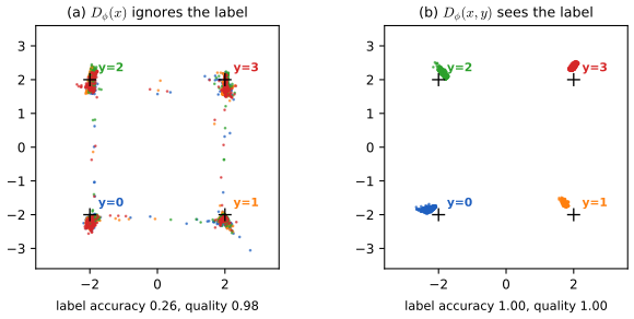
A label-blind critic cannot enforce the conditioning. If \(D_{\bm\phi}(\bm x)\) ignores \(\bm y\), its optimum compares the marginals \(p^*(\bm x)=\E_{p(\bm y)}p^*(\bm x\given\bm y)\) and \(q_{\bm\theta}(\bm x)\). A generator that ignores its label input and samples from \(p^*(\bm x)\) has \(\JSD=0\) for the marginals but \(\E_y\JSD(p^*(\cdot\given y),p^*(\cdot))>0\) as soon as the class-conditionals differ (the discrete example confirms this): the unconditional game cannot distinguish it from the right answer. In Figure x26.d four Gaussian classes sit at the corners of a square; with the label given to the generator only, the generated samples are realistic (98% within \(4\sigma\) of some class) but only 26% fall at the requested class (chance is 25%); with the label given to the critic as well, all do (100% and 100%).
26.5 Inference with GANs
pp. 913–914 Unlike a VAE, a GAN has no encoder: it defines no \(p(\bm z\given\bm x)\). Approaches combine GANs with VAEs (hybrid methods) or build inference methods for implicit models (Dumoulin et al., 2017; Donahue et al., 2017; an overview is Huszar, 2017). In BiGAN (bidirectional GAN) or ALI (adversarially learned inference) an implicit encoder \(E_{\bm\zeta}\) maps \(\bm x\) to \(\bm z\) and a discriminator \(D_{\bm\phi}\) learns to separate pairs: \((\bm x,E_{\bm\zeta}(\bm x))\) with \(\bm x\sim p^*\) is "real", \((G_{\bm\theta}(\bm z),\bm z)\) with \(\bm z\sim q(\bm z)\) is "fake" (the book's Figure 26.9, a diagram). The game matches the two joint distributions, so the marginal \(q_{\bm\theta}(\bm x)\) should learn \(p^*(\bm x)\) and the encoder's conditional should learn the generative model's posterior \(q_{\bm\theta}(\bm z\given\bm x)\propto q_{\bm\theta}(\bm x\given\bm z)q(\bm z)\), with no reconstruction loss; at global optimality encoder and decoder are inverses of each other. (Section 21.2.4 explains how VAEs match \(p^*(\bm x)p_\zeta(\bm z\given\bm x)\) to \(p(\bm z)p_\theta(\bm x\given\bm z)\) with an explicit model.)
Filling the gap 26.13: the BiGAN optimum: matching joints gives the marginals, the posterior and (for deterministic maps) the inverse pp. 913–914
Proof
Let \(P_E(\bm x,\bm z)=p^*(\bm x)\,e_{\bm\zeta}(\bm z\given\bm x)\) and \(P_G(\bm x,\bm z)=q(\bm z)\,g_{\bm\theta}(\bm x\given\bm z)\) be the two joint distributions (for a deterministic generator \(g_{\bm\theta}(\cdot\given\bm z)=\delta_{G_{\bm\theta}(\bm z)}\)). The game on pairs is the game of gap 26.2 with data \(P_E\) and model \(P_G\): with the optimal discriminator \(D^*=\frac{P_E}{P_E+P_G}\) the value is \(\JSD(P_E,P_G)-\log2\), minimised (to \(-\log2\)) iff \(P_E=P_G\). Then:
(i) marginals: integrating out \(\bm z\), \(p^*(\bm x)=q_{\bm\theta}(\bm x)\) (the generator learns the data distribution), and integrating out \(\bm x\), the encoder's aggregate posterior \(\int p^*(\bm x)e(\bm z\given\bm x)\d\bm x\) equals the prior \(q(\bm z)\); (ii) conditionals: dividing by \(p^*(\bm x)=q_{\bm\theta}(\bm x)\), \(e_{\bm\zeta}(\bm z\given\bm x)=q_{\bm\theta}(\bm z\given\bm x)\), the true posterior of the implicit model; (iii) inverse maps: if \(G_{\bm\theta}\) and \(E_{\bm\zeta}\) are deterministic, \(P_E\) is carried by the graph \(A=\{(\bm x,\bm z):\bm z=E(\bm x)\}\) and \(P_G\) by the graph \(B=\{(\bm x,\bm z):\bm x=G(\bm z)\}\). If \(P_E=P_G\), then \(P_G(A)=P_E(A)=1\), i.e. \(\Pr_{\bm z\sim q}[E(G(\bm z))=\bm z]=1\), and likewise \(P_E(B)=1\), i.e. \(\Pr_{\bm x\sim p^*}[G(E(\bm x))=\bm x]=1\): the maps are inverse of each other almost surely, without any reconstruction term. (The book writes \(E_\theta(G_\zeta(\bm z))=\bm z\) with the subscripts of the two networks exchanged.)
Finite check: take \(n=4\) points, a random permutation \(G\), the latent distribution chosen so that the marginals match, and run over all \(4!=24\) deterministic encoders \(E\). The joint distributions coincide for exactly one of them, \(E=G^{-1}\), and for no other. For such a discrete space matching the joints is a necessary and sufficient condition for inverse maps; for continuous spaces the statements hold almost surely, and in practice the optimum is only approached.
26.6 Neural architectures in GANs
pp. 914–918 The progress of GANs owes as much to architectures as to losses. The discriminator is rarely optimal, so GANs do not minimise a fixed divergence in practice: the critic is part of a learned loss for the generator that changes with every update, unlike the fixed loss of maximum likelihood. Convolutional critics for images, recurrent critics for sequences, and their regularisation, shape the generator's gradient and are a main driver of quality (Section 26.6.1). The figures of this section (DCGAN generator and discriminator, attention maps, LapGAN, ProgressiveGAN) are architecture diagrams or outputs of large trained models and are not reproduced.
26.6.2 Architectural inductive biases. p. 915 DCGAN (Radford et al., 2016) found a set of guidelines that gave a large gain without changing the learning principle: convolutional generator (Figure 26.10: a projection and reshape followed by strided transposed convolutions) and critic (Figure 26.11), batch normalisation in both, strided convolutions instead of pooling, ReLU in the generator and LeakyReLU in the discriminator. Residual convolutional layers became standard (Gulrajani et al., 2017), and recurrent ones for text (Section 26.7.4).
26.6.3 Attention in GANs. pp. 915–916 In the self-attention GAN (SAGAN, Zhang et al., 2019) both players see a global view of the features instead of a local convolutional neighbourhood (Figure 26.12: query points attending to distant regions). For features \(\bm h\in\R^{C\times N}\) (\(N\) positions): \(\bm f=\bm W_f\bm h\), \(\bm g=\bm W_g\bm h\), \(\bm S=\bm f^\T\bm g\in\R^{N\times N}\), \(\bm\beta=\text{row softmax}(\bm S)\), \(\bm o=\bm W_o(\bm W_h\bm h)\bm\beta^\T\), and the output \(\bm y=\gamma\bm o+\bm h\) with a learned scalar \(\gamma\) (\(\bm W_f,\bm W_g,\bm W_h\in\R^{C'\times C}\), \(\bm W_o\in\R^{C\times C'}\), \(C'\le C\)). With \(\gamma=0\) the layer is the identity, so adding attention does not shrink the set of functions an architecture can express, and it adds four weight matrices per layer; that more parameters help is a repeated empirical observation. The layer is attention as kernel regression (gap 16.7); gap 26.14 records the properties used here.
26.6.4 Progressive generation. pp. 916–917 Generating high-resolution colour images directly is hard, so one generates at low resolution and refines. LapGAN (Denton et al., 2015) uses a Laplacian pyramid: a sample at one resolution is upsampled (smoothly) and a conditional generator adds a residual to it to give the next resolution (Figure 26.13); a separate generator and critic are trained per level. ProgressiveGAN (Karras et al., 2018) grows one generator and one critic: new layers are added on top of the low-resolution networks, and a residual connection from the upsampled lower-resolution output is annealed from 0 to 1 (a fade-in) so that training moves smoothly from the old output to the new (Figure 26.14).
26.6.5 Regularization. pp. 917–918 Regularisation of generator and discriminator is justified by theory (it is tied to the convergence analysis: gap 26.11), by practice and by the wish to avoid overfitting. Methods: noise added to the discriminator's input (Arjovsky and Bottou, 2017) or to its hidden features, batch normalisation, dropout in the discriminator, spectral normalisation (Miyato et al., 2018) and gradient penalties on \(\|\nabla_{\bm x}D_{\bm\phi}(\bm x)\|_2\) (Gulrajani et al., 2017; Arjovsky et al., 2017; Mescheder et al., 2018). Stability and performance can pull in opposite directions: too much regularisation gives very stable but worse models (Brock et al., 2019).
26.6.6 Scaling up GAN models. p. 918 BigGAN (Brock et al., 2019), StyleGAN (Karras et al., 2020) and alias-free GAN (Karras et al., 2021) combine very large residual networks, self-attention, spectral normalisation in both players, batch normalisation in the generator and large batch sizes. The losses, parameterisations and optimisation have to be considered together.
Filling the gap 26.14: the self-attention layer, spectral normalisation as a Lipschitz bound, and the gradient penalty pp. 915–918, Sections 26.6.3 and 26.6.5
Proof
Self-attention (26.6.3). The rows of \(\bm\beta\) are probability vectors (softmax), so column \(j\) of \((\bm W_h\bm h)\bm\beta^\T\) is a convex combination of the transformed features, with weights \(\beta_{ji}\) depending on how well the query \(\bm f_j\) matches the keys \(\bm g_i\): each position gets a weighted average over all positions, a global receptive field in one layer. If the positions are permuted by \(\bm P\), \(\bm h\mapsto\bm h\bm P\), then \(\bm S\mapsto\bm P^\T\bm S\bm P\), the row softmax commutes with the simultaneous permutation, and \(\bm y\mapsto\bm y\bm P\): the layer is permutation equivariant (convolutions are only translation equivariant; position information must be supplied separately). With \(\gamma=0\), \(\bm y=\bm h\). All three properties, and the shapes above, were checked numerically on a random layer (\(C=6\), \(C'=3\), \(N=10\)).
Spectral normalisation as a Lipschitz bound (26.6.5). A critic \(D(\bm x)=\bm W_L\,a(\bm W_{L-1}\cdots a(\bm W_1\bm x))\) with activations \(a\) that are 1-Lipschitz (ReLU, LeakyReLU with slope in \([0,1]\)) satisfies \(\|D(\bm x)-D(\bm x')\|\le\prod_{l}\|\bm W_l\|_2\,\|\bm x-\bm x'\|\), where the operator norm \(\|\bm W\|_2=\sigma_{\max}(\bm W)\) is the largest singular value: a composition of Lipschitz maps has Lipschitz constant at most the product. Dividing every \(\bm W_l\) by \(\sigma_{\max}(\bm W_l)\) makes each factor 1, so the critic is 1-Lipschitz, the constraint of (26.31) and (26.33). This is sufficient, not necessary (the bound ignores that the activation patterns and singular directions do not align, so it can be loose). For three random LeakyReLU layers with unit spectral norms the largest ratio \(|D(\bm x)-D(\bm x')|/\|\bm x-\bm x'\|\) over 2000 random pairs was 0.11, which shows how loose the bound can be. \(\sigma_{\max}\) is estimated by power iteration: \(\bm v\leftarrow\bm W^\T\bm u/\|\bm W^\T\bm u\|\), \(\bm u\leftarrow\bm W\bm v/\|\bm W\bm v\|\), \(\sigma\approx\bm u^\T\bm W\bm v\); the error contracts by the factor \((\sigma_2/\sigma_1)^2\) per sweep (if the start has a component along the top singular vector), and with warm starts one sweep per training step suffices.
Gradient penalties. The two penalties in the literature target different things. The R1 penalty \(\tfrac\gamma2\E_{p^*}\|\nabla_{\bm x}D\|^2\) at real data is the one analysed in gap 26.11: in DiracGAN it is \(\tfrac\gamma2\phi^2\) and adds damping \(-\gamma/2\) to the eigenvalues. The Wasserstein penalty \(\lambda\,\E_{\hat{\bm x}}(\|\nabla_{\bm x}D(\hat{\bm x})\|-1)^2\) at random points \(\hat{\bm x}\) on segments between data and generated samples pushes the critic towards unit slope there, which is where the optimal 1-Lipschitz critic has unit slope along the optimal transport paths (Result 17.11). The penalty is a soft constraint: it does not guarantee a 1-Lipschitz critic, and so, like (26.31), gives no guarantee that the objective bounds \(W_1\) from below.
26.7 Applications
p. 918 The ability to generate plausible data supports many applications; the book surveys images, video, audio and text, imitation learning, domain adaptation and art. They are described here in brief, with the one piece of mathematics the book states (the CycleGAN loss) treated in gap 26.15.
26.7.1 GANs for image generation
pp. 918–921 Image generation is the most studied application; a survey of the theory is Goodfellow (2016). Generating faces needs a large pretrained GAN, so it is not reproduced here. Figure 26.15 shows the progression of face quality from the original GAN through DCGAN, CoupledGAN, ProgressiveGAN and StyleGAN; it consists of photographs and is not reproduced. The book also points to the risks of synthetic media and deepfakes.
26.7.1.1 Conditional image generation. BigGAN generates class-conditional ImageNet samples; StyleGAN learns a conditioning "style" vector on top of the ProgressiveGAN architecture, and interpolating between styles lets coarse attributes (pose, face shape) come from one sample and fine ones (hair style) from another.
26.7.1.2 Paired image-to-image generation. When \(\bm y\) has the shape of \(\bm x\) (colourisation, edges to photos, aerial photos to maps) the conditional model \(q_{\bm\theta}(\bm x\given\bm y)\) of Section 26.4 translates between domains. pix2pix (Isola et al., 2017) uses a U-net generator with instance normalisation and a PatchGAN discriminator that classifies local patches as real or fake: the critic then judges texture and style rather than global content, is faster to train and gives a denser feedback signal (Figure 26.16, photographs of results, not reproduced).
26.7.1.3 Unpaired image-to-image generation. Paired data are expensive; often one has only \(\mathcal D_x=\{\bm x_n\}\) and \(\mathcal D_y=\{\bm y_n\}\) from two domains (day and night images). Fitting a joint \(p(\bm x,\bm y)\) from two marginals is ill-posed (infinitely many joints have the given marginals), so one adds constraints. With generators \(G:\mathcal X\to\mathcal Y\) and \(F:\mathcal Y\to\mathcal X\) one asks them to be inverses of each other, the cycle-consistency loss (Zhu et al., 2017), \[ L_{\rm cycle}=\E_{p(\bm x)}\|F(G(\bm x))-\bm x\|_1+\E_{p(\bm y)}\|G(F(\bm y))-\bm y\|_1, \tag{26.64} \] and optionally that a generator leave samples of its own target domain unchanged (identity loss), \[ L_{\rm identity}=\E_{p(\bm x)}\|\bm x-F(\bm x)\|_1+\E_{p(\bm y)}\|\bm y-G(\bm y)\|_1, \tag{26.65} \] together with two discriminators \(D_X,D_Y\) and any GAN loss \(L_{\rm GAN}\) to make the outputs of \(G\) look like samples of \(p(\bm y)\) and those of \(F\) like samples of \(p(\bm x)\) (Figures 26.17 and 26.18, a diagram and photographs). The CycleGAN objective is \[ L=L_{\rm GAN}+\lambda_1L_{\rm cycle}+\lambda_2L_{\rm identity}. \tag{26.66} \]
Filling the gap 26.15: what cycle consistency and the identity loss do and do not determine pp. 920–921, (26.64)–(26.66)
Proof
The general statement (cycle consistency alone does not select a translation; it only requires \(F=G^{-1}\) on the data) is Result 17.12 of the deep-learning course. A closed-form example makes it concrete and shows what the identity loss adds. Let \(x\sim\N(0,1)\) and \(y\sim\N(0,\sigma^2)\), \(\sigma=2\). Both \(G_+(x)=\sigma x\) and \(G_-(x)=-\sigma x\) push \(p(x)\) onto \(p(y)\) (the Gaussian is symmetric), so the adversarial loss cannot tell them apart; with \(F_\pm=G_\pm^{-1}\) the cycle loss (26.64) is exactly 0 for both. They define different joint distributions: \(G_+\) is the monotone (optimal-transport) map, \(G_-\) its mirror image. The identity loss (26.65) does separate them: for \(G_\pm\), with \(F_\pm(y)=\pm y/\sigma\), \[ L_{\rm identity}=\E|x\mp x/\sigma|+\E|y\mp\sigma y|=|1\mp\tfrac1\sigma|\,\E|x|+|1\mp\sigma|\,\E|y|,\qquad\E|x|=\sqrt{2/\pi},\ \E|y|=\sigma\sqrt{2/\pi}, \] which is \(\sqrt{2/\pi}\,[\,|1-\tfrac12|+2\,|1-2|\,]=1.995\) for \(G_+\) and \(\sqrt{2/\pi}\,[\tfrac32+2\cdot3]=5.985\) for \(G_-\) (a simulation with \(4\times10^5\) draws gives 1.99 and 5.98). The identity loss prefers the map that moves points the least, here the monotone one. But the preference is a property of the loss, not something the data determine, and it breaks ties only between maps that already satisfy the adversarial and cycle constraints; with several domains and non-symmetric distributions many cycle-consistent maps remain, which is why such models can hide information in the output (steganography) and fail on shapes.
26.7.2 Video generation
pp. 921–922 The framework extends from frames to videos. The extra requirement is spatio-temporal consistency, obtained by letting a discriminator see the real and generated sequences in order, so that realistic frames in the wrong order are penalised; a second discriminator on single frames can ensure each frame is realistic; the generator needs a temporal element, often recurrent. Video-to-video translation and motion transfer follow.
26.7.3 Audio generation
p. 922 Autoregressive models (WaveNet, WaveRNN) generate audio well but sequentially, which is slow. GANs offer parallel generation: GANSynth for single notes, GAN vocoders from mel-spectrograms, voice conversion with a modified CycleGAN, WaveGAN for raw audio, and text-to-speech GANs (first with one-dimensional convolutions in the manner of conditional image GANs, then GAN-TTS with discriminators at several frequency scales that matches autoregressive models in mean opinion score).
26.7.4 Text generation
pp. 922–923 Text is discrete, so GANs for text are explicit models (they model the probability of the output), unlike the continuous implicit GANs above. Maximum likelihood with autoregressive models is the default; GANs allow non-autoregressive, one-shot generation. The GAN losses (26.19), (26.21), (26.28) contain terms \(\E_{q_{\bm\theta}}f(\bm x)\) that we must both evaluate and differentiate in \(\bm\theta\). For continuous \(\bm x\) the reparameterisation (26.49) does this; for discrete \(\bm x\) there is no differentiable map from noise to data, and one resorts to the score-function estimator (Section 6.3.4), whose variance is large (gap 26.9). Common remedies: pre-train the generator by maximum likelihood and fine-tune adversarially for few epochs with small steps (SeqGAN, MaliGAN, RankGAN), which stays close to the maximum-likelihood solution; stabilise the estimator with large batches and discriminator regularisation (ScratchGAN); or use continuous relaxations and curriculum learning without pre-training (a character-level model), possibly with relation networks. Unsupervised style transfer for text uses adversarial classifiers or per-style encoders.
26.7.5 Imitation learning
p. 923 Imitation learning learns policies or rewards from expert demonstrations by minimising a discrepancy between learned and expert behaviour: behavioural cloning treats it as supervised learning, inverse reinforcement learning infers a reward. GANs avoid designing the discrepancy: generative adversarial imitation learning (GAIL, Ho and Ermon, 2016) learns a stochastic policy (the generator) together with a discriminator between agent and expert trajectories that serves as the reward signal. As in Section 26.2, the Jensen–Shannon divergence of the standard loss can be replaced by other \(f\)-divergences (a family of variants including f-GAIL, which learns the best \(f\)).
26.7.6 Domain adaptation
p. 924 To correct a shift between a source and a target domain (Chapter 19), GANs avoid choosing a distance. Pixel-level methods translate source images to the target style (pix2pix, CycleGAN); feature-level methods align representations: domain-adversarial training of neural networks and adversarial discriminative domain adaptation (ADDA) train the feature extractor so that a domain discriminator cannot tell source from target features; CyCADA adds cycle-consistency and semantic losses; further extensions use class information or handle different mode frequencies in the two domains.
26.7.7 Design, art and creativity
p. 924 Generative models of images, with style transfer, are used for algorithmic art, where the goal is appealing images rather than generalisation: real-time re-rendering of objects in video in other styles, exploring fashion designs and fabrics, tools in drawing software, and creative work with music, voice, dance and typography.
Supplement S26 (Generative adversarial networks) supplement
The supplement's Chapter 26 (supplement pages 207–210) consists of the chapter title, an empty page and the divider page of Part V ("Discovery"); there is no additional material for this chapter in the draft, so there is nothing to add to the sections above.
Practice problems
The book has no end-of-chapter exercises for Chapter 26, so here are three short problems of my own, with complete solutions (hidden).
Practice problem 26.1 (the optimal discriminator of two Gaussians). The data are \(p^*=\N(0,1)\) and the model \(q=\N(\delta,1)\), \(\delta=2\). (a) Find \(D^*(x)\) and the log density ratio. (b) What is the best accuracy of a classifier that separates data from model samples (equal priors)? (c) Compute \(\JSD(p^*,q)\) and \(V^*\). (d) A logistic regression of the label on \(x\) with 400 000 samples returns slope and intercept; what should they be?
Solution
(a) \(\log\frac{p^*}{q}=-\frac{x^2}2+\frac{(x-\delta)^2}2=-\delta x+\frac{\delta^2}2\), so \(D^*(x)=\sigma(\frac{\delta^2}2-\delta x)=\sigma(2-2x)\): a decreasing logistic curve, equal to \(\tfrac12\) at \(x=\delta/2=1\). (b) The Bayes accuracy with equal priors is \(\tfrac12+\tfrac12\TV(p^*,q)=\tfrac12+\tfrac12(2\Phi(\delta/2)-1)=\Phi(1)=0.8413\) (the rule "say data iff \(x<1\)"). (c) By quadrature (and as in
jsd), \(\JSD=0.3368\) and \(V^*=0.3368-0.6931=-0.3563\); for comparison \(\Dkl(p^*\|q)=\delta^2/2=2\) and \(\TV=0.6827\). (d) Logistic regression with the label 1 for data recovers \(D^*\): slope \(-\delta=-2\) and intercept \(\delta^2/2=2\); for \(\delta=1.5\) a fit on 400 000 points gave slope \(-1.493\) and intercept \(1.119\) against the exact \(-1.5\) and \(1.125\). This is (26.8) in action: the classifier's logit is the log density ratio.Practice problem 26.2 (alternating updates in DiracGAN). For the logistic \(l\) (\(l'(0)=\tfrac12\)) and alternating gradient descent with step \(h\), (a) write the linearised update matrix and its eigenvalues, (b) find the largest \(h\) for which the orbit stays bounded, (c) find the rotation angle and the period for \(h=1\), and (d) say what happens to the spectral radius with the penalty \(\gamma=0.5\) at \(h=0.2\).
Solution
(a) With \(\kappa=hl'(0)=h/2\), \(M=\begin{pmatrix}1&\kappa\\-\kappa&1-\kappa^2\end{pmatrix}\), \(\det M=1\), \(\operatorname{tr}M=2-\kappa^2\); the eigenvalues solve \(\lambda^2-(2-\kappa^2)\lambda+1=0\), \(\lambda=e^{\pm i\omega}\) with \(\cos\omega=1-\kappa^2/2\) when \(\kappa<2\) (gap 26.10). (b) Bounded (a rotation, with the invariant quadratic form \(\phi^2+\theta^2+\kappa\phi\theta\)) iff \(|\operatorname{tr}M|\le2\), i.e. \(\kappa\le2\), \(h\le4\); at \(h=4.4\) the spectral radius is 2.43 and the iterates diverge; at \(h=3.9\) it is exactly 1. (c) \(h=1\): \(\kappa=\tfrac12\), \(\cos\omega=0.875\), \(\omega=0.5054\) rad, period \(2\pi/\omega=12.43\) iterations. (d) With the penalty the update matrix becomes \(\begin{pmatrix}1-h\gamma&h c_0\\-hc_0(1-h\gamma)&1-h^2c_0^2\end{pmatrix}\) (the discriminator step is \(\phi'=(1-h\gamma)\phi+hc_0\theta\), then \(\theta'=\theta-hc_0\phi'\)) with determinant \(1-h\gamma\); for \(h=0.2\), \(\gamma=0.5\) that is 0.9, and the spectral radius is \(\sqrt{0.9}=0.9487\) when the eigenvalues are complex, so the orbit contracts. The code (
lin_map_radius) returns 0.9487; without the penalty the value is 1.Practice problem 26.3 (MMD and Wasserstein between Gaussians). For \(p^*=\N(0,1)\), \(q=\N(\delta,1)\) and the kernel \(\exp(-(x-y)^2/2)\) compute \(\MMD^2\) in closed form, evaluate it at \(\delta=2\), find its behaviour for small and large \(\delta\), and compare with \(W_1\). Check with \(3000\) draws of each.
Solution
For independent \(X\sim\N(m_1,s_1^2)\), \(Y\sim\N(m_2,s_2^2)\), \(\E e^{-(X-Y)^2/2}=\sqrt{1/v}\,e^{-(m_1-m_2)^2/(2v)}\) with \(v=1+s_1^2+s_2^2\) (gap 26.6). Here \(v=3\) in all three terms, so \(\MMD^2=\frac2{\sqrt3}-\frac2{\sqrt3}e^{-\delta^2/6}=\frac2{\sqrt3}(1-e^{-\delta^2/6})\). At \(\delta=2\): \(1.1547\times(1-e^{-2/3})=0.5619\). For small \(\delta\), \(\MMD^2\approx\delta^2/(3\sqrt3)=0.1925\,\delta^2\) (quadratic, like \(W_1^2\) and like the KL divergence \(\delta^2/2\)); for large \(\delta\) it tends to the constant \(2/\sqrt3=1.1547\) and its \(\delta\)-derivative decays like \(\delta e^{-\delta^2/6}\): the same saturation as the JSD, only later (compare \(W_1=\delta\), whose gradient is constant). The unbiased estimator on 3000 draws of each gave 0.557 (the quadrature of the demonstration gives 0.5619). So a generator driven by this MMD has a signal that fades once the model is about 4 standard deviations away, whereas the Wasserstein critic's gradient does not fade (Figure x26.a).
Demonstrations
- Learning by comparison: what a critic sees (Sections 26.2.2–26.2.6): the optimal discriminator, the optimal Wasserstein critic and the MMD witness for a data density and a Gaussian model; KL, JSD, \(\chi^2\), total variation, \(W_1\) and MMD as the model moves.
- DiracGAN: how gradient descent plays a two-player game (Section 26.3.5): simultaneous, alternating and continuous updates, step size, loss and gradient penalty.
- Mode collapse and mode hopping in GAN training (Sections 26.3.3, 26.3.4): replay seven training variants on the sixteen-mode problem.
Python code for every figure: code index. Data used by the demonstrations: data/ch26-modes.json (the other two demonstrations compute everything in the page). Companion demos: Volume 1 and the deep-learning course.
Notes on the book
Points where the book is imprecise or wrong
- (26.4) and (26.9). The divergence (26.4) and the value \(V(q_{\bm\theta},p^*)\) of (26.9) are written with "arg max"; they are the maximal values (the maximiser is the critic).
- Section 26.1. "The generating procedure defines a valid density on the output space" holds for \(m\ge d\) with a full-rank Jacobian; for the case the chapter treats (\(d>m\)) the law is singular and has no density (gap 26.1).
- Table 26.2. The row labelled JSD, \(f=u\log u-(u+1)\log\frac{u+1}2\), gives \(D_f=2\JSD\) in the normalisation (26.16) (\(\JSD=\frac12\Dkl(p\|m)+\frac12\Dkl(q\|m)\)); the original GAN is its \(f\)-GAN with \(t=\log2D\), and the conjugate of the Pearson row is printed as a function of \(u\) instead of \(t\) (gap 26.4).
- Section 26.3.1, the list of \((g,h,l)\). For the original and non-saturating GANs \(g,h,l\) are losses to be minimised as in (26.43); for the Wasserstein row (\(g=t\), \(h=-t\), \(l=t\)) and the \(f\)-divergence row (\(g=t\), \(h=-f^\dagger(t)\), \(l=f^\dagger(t)\)) they are the signs of the objective that the critic maximises in (26.32) and (26.27), so with (26.43) the signs should be reversed (\(g=-t\), \(h=t\), \(l=-t\) for the Wasserstein GAN) or the critic is the negative of the one in (26.33).
- (26.48). The left side is written \(L_G(\bm\phi,\bm\theta)\); it should be \(\nabla_{\bm\theta}L_G(\bm\phi,\bm\theta)\).
- Algorithm 26.2, line 6. The discriminator gradient is written \(\nabla_{\bm\phi}\frac1M\sum[g(D_{\bm\phi}(\bm x_m))+\nabla_{\bm\phi}h(D_{\bm\phi}(G_{\bm\theta}(\bm z_m)))]\) with a second \(\nabla_{\bm\phi}\) inside the sum; one gradient of the whole average is meant.
- (26.50)–(26.51). With \(l(z)=-\log(1+e^{-z})\) and \(L_D=-l(0)-l(\theta\phi)\), descent on \(\phi\) raises \(\theta\phi\), the logit of the generated point, so the "discriminator" rewards the fake sample and the roles are exchanged. With \(l(z)=-\log(1+e^{z})\) (\(l'(0)=-\tfrac12\)), or equivalently \(\theta\mapsto-\theta\), they are the standard ones. The conclusions (eigenvalues \(\pm il'(0)\), the conserved radius) hold for any \(l\) and are unaffected; our code and demonstration follow the book's \(l\).
- (26.59). The entries are written with an added \(l(0)\) inside the second derivatives (\(\nabla_\phi\nabla_\phi l(\theta\phi)+l(0)\), etc.); the constant \(l(0)\) has zero derivative and the entries are just the second derivatives of \(\pm l(\theta\phi)\), which vanish at \(\theta=\phi=0\) except for the cross terms \(\pm l'(0)\).
- Section 26.3.5, Nash equilibrium. "Given an optimal discriminator, the data distribution is the optimal generator as it is the minimiser of the JSD": against the fixed \(D=\frac12\) every generator is a best response; \(q=p^*\) is the unique minimiser only of \(\min_q\max_DV\) (gap 26.11).
- Section 26.5. "\(E_\theta(G_\zeta(\bm z))=\bm z\) and \(G_\zeta(E_\theta(\bm x))=\bm x\)": the subscripts are exchanged (the generator is \(G_{\bm\theta}\), the encoder \(E_{\bm\zeta}\)); the statement holds almost surely and for deterministic maps (gap 26.13).
- Section 26.2.6. That the generator "minimises a lower bound of the divergence" is stated as a risk; it is the exact reason why a restricted critic can stall (the example of gap 26.4 has the KL bound equal to 0 for every \(s\)).
References
- Murphy, K. P. (2023). Probabilistic Machine Learning: Advanced Topics. MIT Press, Cambridge, MA. Chapter 26, pp. 893–924, and supplementary material, Chapter 26. probml.github.io/pml-book/book2.html.
- Arjovsky, M. and Bottou, L. (2017). Towards principled methods for training generative adversarial networks. International Conference on Learning Representations.
- Arjovsky, M., Chintala, S. and Bottou, L. (2017). Wasserstein generative adversarial networks. International Conference on Machine Learning.
- Balduzzi, D., Racaniere, S., Martens, J., Foerster, J., Tuyls, K. and Graepel, T. (2018). The mechanics of n-player differentiable games. International Conference on Machine Learning.
- Brock, A., Donahue, J. and Simonyan, K. (2019). Large scale GAN training for high fidelity natural image synthesis. International Conference on Learning Representations.
- Chavdarova, T., Gidel, G., Fleuret, F. and Lacoste-Julien, S. (2019). Reducing noise in GAN training with variance reduced extragradient. Advances in Neural Information Processing Systems, 32.
- Denton, E., Chintala, S., Szlam, A. and Fergus, R. (2015). Deep generative image models using a Laplacian pyramid of adversarial networks. Advances in Neural Information Processing Systems, 28.
- Donahue, J., Krähenbühl, P. and Darrell, T. (2017). Adversarial feature learning. International Conference on Learning Representations.
- Dumoulin, V., Belghazi, I., Poole, B., Mastropietro, O., Lamb, A., Arjovsky, M. and Courville, A. (2017). Adversarially learned inference. International Conference on Learning Representations.
- Dziugaite, G. K., Roy, D. M. and Ghahramani, Z. (2015). Training generative neural networks via maximum mean discrepancy optimization. Uncertainty in Artificial Intelligence.
- Endres, D. M. and Schindelin, J. E. (2003). A new metric for probability distributions. IEEE Transactions on Information Theory, 49(7), 1858–1860.
- Farnia, F. and Ozdaglar, A. (2020). GANs may have no Nash equilibria. arXiv:2002.09124.
- Fedus, W., Rosca, M., Lakshminarayanan, B., Dai, A. M., Mohamed, S. and Goodfellow, I. (2018). Many paths to equilibrium: GANs do not need to decrease a divergence at every step. International Conference on Learning Representations.
- Goodfellow, I. (2016). NIPS 2016 tutorial: generative adversarial networks. arXiv:1701.00160.
- Goodfellow, I., Pouget-Abadie, J., Mirza, M., Xu, B., Warde-Farley, D., Ozair, S., Courville, A. and Bengio, Y. (2014). Generative adversarial nets. Advances in Neural Information Processing Systems, 27.
- Gulrajani, I., Ahmed, F., Arjovsky, M., Dumoulin, V. and Courville, A. (2017). Improved training of Wasserstein GANs. Advances in Neural Information Processing Systems, 30.
- Ho, J. and Ermon, S. (2016). Generative adversarial imitation learning. Advances in Neural Information Processing Systems, 29.
- Huszar, F. (2017). Variational inference using implicit distributions. arXiv:1702.08235.
- Isola, P., Zhu, J.-Y., Zhou, T. and Efros, A. A. (2017). Image-to-image translation with conditional adversarial networks. IEEE Conference on Computer Vision and Pattern Recognition.
- Karras, T., Aila, T., Laine, S. and Lehtinen, J. (2018). Progressive growing of GANs for improved quality, stability, and variation. International Conference on Learning Representations.
- Karras, T., Laine, S., Aittala, M., Hellsten, J., Lehtinen, J. and Aila, T. (2020). Analyzing and improving the image quality of StyleGAN. IEEE Conference on Computer Vision and Pattern Recognition. Karras, T., Aittala, M., Laine, S., Härkönen, E., Hellsten, J., Lehtinen, J. and Aila, T. (2021). Alias-free generative adversarial networks. Advances in Neural Information Processing Systems, 34.
- Karras, T., Laine, S. and Aila, T. (2019). A style-based generator architecture for generative adversarial networks. IEEE Conference on Computer Vision and Pattern Recognition.
- Kingma, D. P. and Ba, J. (2015). Adam: a method for stochastic optimization. International Conference on Learning Representations.
- Li, C.-L., Chang, W.-C., Cheng, Y., Yang, Y. and Póczos, B. (2017). MMD GAN: towards deeper understanding of moment matching network. Advances in Neural Information Processing Systems, 30.
- Li, Y., Swersky, K. and Zemel, R. (2015). Generative moment matching networks. International Conference on Machine Learning.
- Mao, X., Li, Q., Xie, H., Lau, R. Y. K., Wang, Z. and Smolley, S. P. (2017). Least squares generative adversarial networks. IEEE International Conference on Computer Vision.
- Mescheder, L., Nowozin, S. and Geiger, A. (2017). The numerics of GANs. Advances in Neural Information Processing Systems, 30.
- Mescheder, L., Geiger, A. and Nowozin, S. (2018). Which training methods for GANs do actually converge? International Conference on Machine Learning.
- Metz, L., Poole, B., Pfau, D. and Sohl-Dickstein, J. (2017). Unrolled generative adversarial networks. International Conference on Learning Representations.
- Mirza, M. and Osindero, S. (2014). Conditional generative adversarial nets. arXiv:1411.1784.
- Miyato, T., Kataoka, T., Koyama, M. and Yoshida, Y. (2018). Spectral normalization for generative adversarial networks. International Conference on Learning Representations. Miyato, T. and Koyama, M. (2018). cGANs with projection discriminator. International Conference on Learning Representations.
- Nagarajan, V. and Kolter, J. Z. (2017). Gradient descent GAN optimization is locally stable. Advances in Neural Information Processing Systems, 30.
- Nguyen, X., Wainwright, M. J. and Jordan, M. I. (2010). Estimating divergence functionals and the likelihood ratio by convex risk minimization. IEEE Transactions on Information Theory, 56(11), 5847–5861.
- Nowozin, S., Cseke, B. and Tomioka, R. (2016). f-GAN: training generative neural samplers using variational divergence minimization. Advances in Neural Information Processing Systems, 29.
- Odena, A., Olah, C. and Shlens, J. (2017). Conditional image synthesis with auxiliary classifier GANs. International Conference on Machine Learning.
- Pearson, K. (1936). Method of moments and method of maximum likelihood. Biometrika, 28, 34–59.
- Radford, A., Metz, L. and Chintala, S. (2016). Unsupervised representation learning with deep convolutional generative adversarial networks. International Conference on Learning Representations.
- Ratliff, L. J., Burden, S. A. and Sastry, S. S. (2016). On the characterization of local Nash equilibria in continuous games. IEEE Transactions on Automatic Control, 61(8), 2301–2307.
- Ravuri, S., Mohamed, S., Rosca, M. and Vinyals, O. (2018). Learning implicit generative models with the method of learning moments. International Conference on Machine Learning.
- Reid, M. D. and Williamson, R. C. (2011). Information, divergence and risk for binary experiments. Journal of Machine Learning Research, 12, 731–817.
- Qin, C., Wu, Y., Springenberg, J. T., Brock, A., Donahue, J., Lillicrap, T. P. and Kohli, P. (2020). Training generative adversarial networks by solving ordinary differential equations. Advances in Neural Information Processing Systems, 33.
- Rosca, M. et al. (2021), on the discretisation error of gradient-based GAN training, as cited by Murphy (2023), Section 26.3.5.
- Schaefer, F. and Anandkumar, A. (2019). Competitive gradient descent. Advances in Neural Information Processing Systems, 32.
- Zhang, H., Goodfellow, I., Metaxas, D. and Odena, A. (2019). Self-attention generative adversarial networks. International Conference on Machine Learning.
- Zhu, J.-Y., Park, T., Isola, P. and Efros, A. A. (2017). Unpaired image-to-image translation using cycle-consistent adversarial networks. IEEE International Conference on Computer Vision.
The numerical statements in the text (the pushforward density and the singular case; the optimal discriminator and \(V^*=\JSD-\log2\); the Brier, exponential and hinge optima; the conjugates and optimal critics of Table 26.2 and the factor 2 of its JSD row; the exactness of quadratic critics; the fixed-discriminator gradients of the saturating and non-saturating losses; the one-dimensional Wasserstein critic and the discrete duality; the MMD closed form, estimators and the polynomial-kernel identity; the DiracGAN Jacobian, conserved radius, exact radius law, alternating map and its invariant ellipse, and the stability with a gradient penalty; the two gradient estimators and their variances; the conditional and BiGAN optima; the self-attention and spectral-normalisation statements; the cycle-consistency example; and the trained-network numbers) were confirmed numerically.