Diffusion models
A diffusion model turns data into noise with a fixed, simple corruption process, and learns to run that process backwards. The forward process adds Gaussian noise in many small steps (or, for discrete data, randomly replaces or masks symbols); the reverse process is a learned chain of small denoising steps, trained by a variational bound that reduces to a weighted regression of the added noise, which is the same thing as estimating the score \(\nabla\log q_t\) of every noised marginal. These notes cover the DDPM and its bound, learned noise schedules, score-based models and their equivalence with DDPMs, the continuous-time picture (forward and reverse SDEs, the probability-flow ODE, flow matching), fast samplers (DDIM, distillation), guidance, and discrete diffusion. The demonstrations use data whose noised scores are known exactly, so they isolate what each sampler does.
Ch. 1 Introduction Ch. 2 Probability Ch. 3 Statistics Ch. 4 Graphical models Ch. 5 Information theory Ch. 6 Optimisation Ch. 7 Inference algorithms Ch. 8 Gaussian filtering Ch. 9 Message passing Ch. 10 Variational inference Ch. 11 Monte Carlo Ch. 12 MCMC Ch. 13 Sequential Monte Carlo Ch. 14 Predictive models Ch. 15 GLMs Ch. 16 Deep networks Ch. 17 Bayesian neural networks Ch. 18 Gaussian processes Ch. 19 Beyond iid Ch. 20 Generative models Ch. 21 VAEs Ch. 22 Autoregressive models Ch. 23 Normalizing flows Ch. 24 Energy-based models Ch. 25 Diffusion models Ch. 26 GANs Ch. 27 Discovery methods Ch. 28 Latent factor models Ch. 29 State-space models Ch. 30 Graph learning Ch. 31 Nonparametric Bayes Ch. 32 Representation learning Ch. 33 Interpretability Ch. 34 Decision making Ch. 35 Reinforcement learning Ch. 36 Causality
How to read these notes
They follow the book. Sections carry the book's numbers, and equations the book numbers keep their numbers, e.g. \((25.23)\); equations without a number are steps the book skips. The online supplement's Chapter 25 is a title page with no content, so there are no supplement sections in this chapter.
Filling the gaps. Wherever the book writes "one can show", quotes a result from the literature, or leaves a step to the reader, an orange Filling the gap box gives the full argument. Proofs start hidden: open one with its bar, or use the buttons below. The basic DDPM algebra (the diffusion kernel, the posterior of one step, the ELBO and its noise-prediction form, the best noise predictor, implicit and denoising score matching, the probability-flow ODE) is proved in the deep-learning course and is linked rather than repeated; the boxes here spend their space on what this book adds.
Figures, scale and demonstrations. Every computed figure is reproduced by the Python code, on one CPU thread. Where a figure needs the score of noised data, the data distribution is a Gaussian mixture, whose noised marginals are mixtures again, so the score is exact. Figures 25.4, 25.8 and 25.9 come from GPU-trained image models in the book; my versions are stand-ins on the 8 × 8 handwritten digits of scikit-learn (1 797 images), with small multilayer perceptrons trained in under a minute, and each caption says so. Figure 25.11 (an image slide) is replaced by the exact computation it illustrates. Figures 25.1, 25.3, 25.12 to 25.15 and 25.17 are diagrams or illustrations from papers, and Figure 25.10 shows faces from a large model trained on CelebA-HQ; none is reproduced. Two extra figures (25.x1, 25.x2) illustrate points made here. The ▶ Demo boxes open an interactive demonstration set to the case being discussed.
Main reference
K. P. Murphy, Probabilistic Machine Learning: Advanced Topics, MIT Press (2023; online draft of December 2025), Chapter 25, pages 867–891 (book page: probml.github.io/pml-book/book2.html). Section, equation, figure and algorithm numbers below refer to this book. The explanations, derivations, figures and code are my own. The book has no end-of-chapter exercises for this chapter; three practice problems are given instead.
Companion courses
The deep-learning course covers the DDPM in detail in Chapter 20, Diffusion models: the diffusion kernel (Result 20.2), the reverse conditional given the data (Result 20.3), the ELBO with nothing dropped (Result 20.5) and its noise-prediction form (Result 20.7), the best noise predictor as a rescaled score (Result 20.8), implicit and denoising score matching (Results 20.10, 20.11), the continuous-time limit and the probability-flow ODE (Results 20.12, 20.13) and guidance (Result 20.14). Its demonstrations show the forward process and sampling. Within this course: the ELBO identity (gap 10.1), hierarchical VAEs (Section 21.5), Langevin Monte Carlo (Section 12.5.6), quasi-Monte Carlo (Section 11.6.5), optimal transport (Section 6.8) and the evaluation of generative models (Section 20.4.1). Score matching for energy-based models (the book's Chapter 24) and normalizing flows (Chapter 23) are referred to below by their book numbers.
What this chapter adds: the two natural reverse variances and the sense in which they bound the true one, the weight \(\lambda_t\), the variational diffusion model and its schedule-free continuous loss (with a sign correction), low-discrepancy timesteps, the equivalence of score-based models and DDPMs in both the variance-exploding and variance-preserving forms, the time reversal of an SDE and the family of samplers with the same marginals, flow matching and its likelihood, DDIM as an exact step of a reparameterised ODE, the distillation target, the guided reverse step and the link between the two guidance weights, and discrete diffusion with its closed forms.
The chapter at a glance
- 25.2 The reverse variances \(\beta_t\) and \(\bt_t\) (gap 25.1); the KL terms and \(\lambda_t\) (25.2); the VDM diffusion loss (25.3); low-discrepancy timesteps (25.4).
- 25.3 Why score matching misses mixture weights (gap 25.5); score models are DDPMs (25.6).
- 25.4 The forward SDEs (gap 25.7); the probability-flow ODE and the reverse SDE from the Fokker-Planck equation (25.8); the ODE plus Langevin split (25.9); exact likelihood and identifiability (25.10); flow matching (25.11).
- 25.5 DDIM (gap 25.12); the distillation target (25.13).
- 25.6 The guided reverse step and the two guidance weights (gap 25.14); what classifier-free guidance samples (25.15).
- 25.7 The marginal and posterior of a discrete chain (gap 25.16); the three kernels in closed form (25.17); the \(\bx_0\)-parameterisation (25.18); the schedules (25.19); BERT and masked diffusion (25.20).
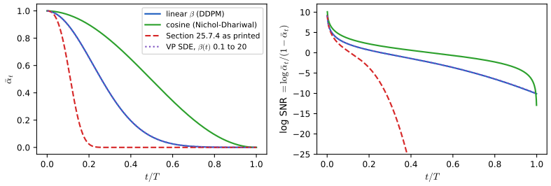
Notation. \(\bx_0\sim q_0\) is a data point and \(\bx_1,\dots,\bx_T\) its noised versions; \(\alpha_t=1-\beta_t\), \(\ab_t=\prod_{s\le t}\alpha_s\); \(\beps\sim\N(\bm 0,\bI)\). In continuous time \(t\in[0,1]\), \(\bx_t=\alpha_t\bx_0+\sigma_t\beps\) and \(\SNR(t)=R(t)=\alpha_t^2/\sigma_t^2\) (the book reuses the letter \(\alpha_t\) here for \(\sqrt{\ab_t}\)). The score of the noised marginal is \(\nabla\log q_t\). All examples use the variance-preserving process with \(\beta(t)\) rising linearly from 0.1 to 20, which is the continuous version of the DDPM schedule \(\beta_t\) from \(10^{-4}\) to 0.02 with \(T=1000\) (Figure 25.x1).
Prerequisites. Chapters 10, 12 and 21 of the book; Gaussian conditioning; for Section 25.4, the Itô formula at the level of a first course.
25.1 Introduction
p. 867 The guiding observation: turning data into noise is easy, turning noise into data is hard, but the second can be learned one small step at a time. A forward (diffusion) process passes \(\bx_0\) through \(T\) steps of a fixed stochastic encoder \(q(\bx_t\given\bx_{t-1})\) until \(\bx_T\) is close to \(\N(\bm 0,\bI)\); a reverse process \(p_{\bm\theta}(\bx_{t-1}\given\bx_t)\), a learned decoder shared across steps, takes noise back to data. Diffusion models are related to VAEs (a hierarchical VAE with a fixed encoder, Chapter 21), to normalizing flows (all latents have the data's dimension, and the ODE version is a continuous flow) and to energy-based models (through score matching).
25.2 Denoising diffusion probabilistic models (DDPMs)
pp. 867–868 The DDPM (Sohl-Dickstein et al., 2015; Ho, Jain and Abbeel, 2020) is a hierarchical latent-variable model with latents \(\bx_{1:T}\) of the same size as \(\bx_0\), a linear Gaussian encoder with no parameters, and one decoder network used at every step. These restrictions make the bound a sum of weighted least-squares problems and remove the posterior collapse of VAEs (Section 21.4).
25.2.1 Encoder (forwards diffusion)
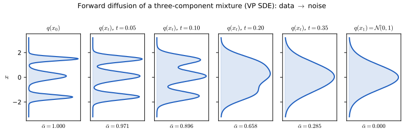
pp. 868–869 The encoder is the linear Gaussian Markov chain \[ q(\bx_t\given\bx_{t-1})=\N\big(\bx_t\given\sqrt{1-\beta_t}\,\bx_{t-1},\beta_t\bI\big),\qquad q(\bx_{1:T}\given\bx_0)=\prod_{t=1}^Tq(\bx_t\given\bx_{t-1}), \tag{25.1-25.2} \] with \(\beta_t\in(0,1)\) from a noise schedule. Its \(t\)-step marginal, the diffusion kernel, is \[ q(\bx_t\given\bx_0)=\N\big(\bx_t\given\sqrt{\ab_t}\,\bx_0,(1-\ab_t)\bI\big),\qquad \alpha_t=1-\beta_t,\quad\ab_t=\textstyle\prod_{s=1}^t\alpha_s, \tag{25.3-25.4} \] (proof by induction: Result 20.2 of the deep-learning course; the variance obeys \(v_t=\alpha_tv_{t-1}+\beta_t\), \(v_0=0\), whose solution is \(1-\ab_t\)). The schedule is chosen with \(\ab_T\approx0\). The unconditional marginal \(q(\bx_t)=\int q_0(\bx_0)q(\bx_t\given\bx_0)\,\d\bx_0\) (25.5) is the data distribution shrunk by \(\sqrt{\ab_t}\) and convolved with \(\N(\bm0,(1-\ab_t)\bI)\), so it gets smoother as \(t\) grows (Figure 25.2). For images, convolving with white noise removes fine detail first (high spatial frequencies have little power and are swamped first) and coarse structure last.
25.2.2 Decoder (reverse diffusion)
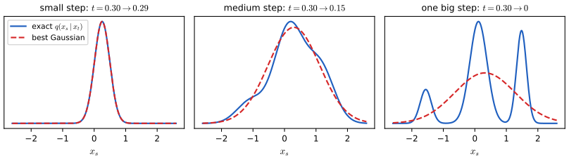
p. 869 Given \(\bx_0\), one forward step can be reversed exactly by Gaussian conditioning (Result 20.3 of the deep-learning course): \[ q(\bx_{t-1}\given\bx_t,\bx_0)=\N\big(\bx_{t-1}\given\tilde\bmu_t(\bx_t,\bx_0),\bt_t\bI\big),\quad \tilde\bmu_t=\frac{\sqrt{\ab_{t-1}}\beta_t}{1-\ab_t}\bx_0+\frac{\sqrt{\alpha_t}(1-\ab_{t-1})}{1-\ab_t}\bx_t,\quad \bt_t=\frac{1-\ab_{t-1}}{1-\ab_t}\beta_t. \tag{25.6-25.8} \] The generator does not know \(\bx_0\), so it uses \(p_{\bm\theta}(\bx_{t-1}\given\bx_t)=\N(\bx_{t-1}\given\bmu_{\bm\theta}(\bx_t,t),\bm\Sigma_{\bm\theta}(\bx_t,t))\) (25.9), usually with \(\bm\Sigma=\sigma_t^2\bI\), and \(p_{\bm\theta}(\bx_{0:T})=p(\bx_T)\prod_tp_{\bm\theta}(\bx_{t-1}\given\bx_t)\), \(p(\bx_T)=\N(\bm0,\bI)\). A Gaussian reverse step is justified when \(\beta_t\) is small (Result 20.4 of the deep-learning course; Figure 25.11 below shows what goes wrong for large steps). The two standard choices \(\sigma_t^2=\beta_t\) and \(\sigma_t^2=\bt_t\) are explained next.
Filling the gap 25.1: the reverse variances \(\beta_t\) and \(\bt_t\) as the two extreme cases p. 869, (25.9)
Proof
Claim. Let \(\bm c_t=\sqrt{\ab_{t-1}}\beta_t/(1-\ab_t)\) be the coefficient of \(\bx_0\) in \(\tilde\bmu_t\). For any data distribution, the true reverse step \(q(\bx_{t-1}\given\bx_t)\) has covariance \[ \cov(\bx_{t-1}\given\bx_t)=\bt_t\bI+c_t^2\cov(\bx_0\given\bx_t). \] Hence (i) it equals \(\bt_t\bI\) when the data are a point mass, and is always at least \(\bt_t\bI\); (ii) it equals \(\beta_t\bI\) when \(q_0=\N(\bm0,\bI)\); (iii) for any data with \(\cov(\bx_0)\preceq\bI\), its average over \(\bx_t\) is at most \(\beta_t\bI\).
The decomposition. By the Markov property, \(q(\bx_{t-1}\given\bx_t)=\int q(\bx_{t-1}\given\bx_t,\bx_0)q(\bx_0\given\bx_t)\,\d\bx_0\). The law of total covariance, conditioning on \(\bx_0\) inside the law given \(\bx_t\), gives \(\cov(\bx_{t-1}\given\bx_t)=\E[\cov(\bx_{t-1}\given\bx_t,\bx_0)\given\bx_t]+\cov(\E[\bx_{t-1}\given\bx_t,\bx_0]\given\bx_t)=\bt_t\bI+\cov(c_t\bx_0+(\cdot)\bx_t\given\bx_t)=\bt_t\bI+c_t^2\cov(\bx_0\given\bx_t)\), since the \(\bx_t\) term is fixed given \(\bx_t\). The second term is positive semidefinite, which gives the lower bound, attained when \(\bx_0\) is known (a point mass).
Gaussian data. If \(q_0=\N(\bm0,\bI)\), then \(\bx_t=\sqrt{\ab_t}\bx_0+\sqrt{1-\ab_t}\beps\) has covariance \(\bI\), and \(\cov(\bx_0\given\bx_t)=\bI-\ab_t\bI=(1-\ab_t)\bI\) by Gaussian conditioning (\(\cov(\bx_0,\bx_t)=\sqrt{\ab_t}\bI\)). Then \(\bt_t+c_t^2(1-\ab_t)=\frac{\beta_t}{1-\ab_t}\big[(1-\ab_{t-1})+\ab_{t-1}\beta_t\big]=\frac{\beta_t}{1-\ab_t}\big[1-\ab_{t-1}\alpha_t\big]=\beta_t\). (Directly: every \(q(\bx_t)\) is \(\N(\bm0,\bI)\), the pair \((\bx_{t-1},\bx_t)\) has cross-covariance \(\sqrt{\alpha_t}\bI\), so \(\bx_{t-1}\given\bx_t\sim\N(\sqrt{\alpha_t}\bx_t,\beta_t\bI)\): the chain is reversible.)
Average upper bound. \(\E_{\bx_t}\cov(\bx_0\given\bx_t)\) is the error covariance of the best estimator \(\E[\bx_0\given\bx_t]\), which is no larger than that of the best linear estimator. For \(\cov(\bx_0)=\bm\Sigma_0\) the linear error is \(\bm\Sigma_0-\ab_t\bm\Sigma_0(\ab_t\bm\Sigma_0+(1-\ab_t)\bI)^{-1}\bm\Sigma_0\), increasing in \(\bm\Sigma_0\), and equal to \((1-\ab_t)\bI\) at \(\bm\Sigma_0=\bI\). So for \(\bm\Sigma_0\preceq\bI\), \(\E_{\bx_t}\cov(\bx_{t-1}\given\bx_t)\preceq\bt_t\bI+c_t^2(1-\ab_t)\bI=\beta_t\bI\). This is the precise sense of Ho et al.'s statement that the two choices are lower and upper bounds (it holds on average over \(\bx_t\), not for every \(\bx_t\)). For data \(\pm1\) with equal probability and \(t=100\) of the DDPM schedule, the averaged reverse variance lies strictly between \(\bt_t\) and \(\beta_t\), as confirmed numerically by quadrature. \(\square\)
25.2.3 Model fitting
pp. 870–871 The model is fitted by maximising the ELBO, as for a VAE: \[ \log p_{\bm\theta}(\bx_0)\ge\E_{q(\bx_{1:T}\given\bx_0)}\Big[\log p(\bx_T)+\sum_{t=1}^T\log\frac{p_{\bm\theta}(\bx_{t-1}\given\bx_t)}{q(\bx_t\given\bx_{t-1})}\Big]=\ELBO(\bx_0). \tag{25.10-25.12} \] Writing \(q(\bx_t\given\bx_{t-1})=q(\bx_{t-1}\given\bx_t,\bx_0)q(\bx_t\given\bx_0)/q(\bx_{t-1}\given\bx_0)\) (25.13; Bayes' rule plus the Markov property), the ratios \(q(\bx_{t-1}\given\bx_0)/q(\bx_t\given\bx_0)\) telescope (25.14–25.17) and the negative bound becomes \[ \mathcal L(\bx_0)=\underbrace{\Dkl\big(q(\bx_T\given\bx_0)\|p(\bx_T)\big)}_{L_T}+\sum_{t=2}^T\underbrace{\E_{q(\bx_t\given\bx_0)}\Dkl\big(q(\bx_{t-1}\given\bx_t,\bx_0)\|p_{\bm\theta}(\bx_{t-1}\given\bx_t)\big)}_{L_{t-1}}\underbrace{-\E_{q(\bx_1\given\bx_0)}\log p_{\bm\theta}(\bx_0\given\bx_1)}_{L_0}. \tag{25.18-25.20} \] (Full derivation: Result 20.5 of the deep-learning course; the identity was confirmed here by Monte Carlo on a one-dimensional chain with \(T=4\) and an arbitrary linear Gaussian decoder.) Every term is a KL between Gaussians. Because \(\bx_t=\sqrt{\ab_t}\bx_0+\sqrt{1-\ab_t}\beps\), the posterior mean can be written with the noise, \[ \tilde\bmu_t=\frac{1}{\sqrt{\alpha_t}}\Big(\bx_t-\frac{\beta_t}{\sqrt{1-\ab_t}}\beps\Big), \tag{25.21} \] which suggests predicting the noise: \(\bmu_{\bm\theta}(\bx_t,t)=\frac{1}{\sqrt{\alpha_t}}\big(\bx_t-\frac{\beta_t}{\sqrt{1-\ab_t}}\beps_{\bm\theta}(\bx_t,t)\big)\) (25.22). Then \[ L_{t-1}=\E_{\bx_0,\beps}\Big[\lambda_t\big\|\beps-\beps_{\bm\theta}\big(\sqrt{\ab_t}\bx_0+\sqrt{1-\ab_t}\beps,t\big)\big\|^2\Big]+\const,\qquad \lambda_t=\frac{\beta_t^2}{2\sigma_t^2\alpha_t(1-\ab_t)}, \tag{25.23} \] and dropping the weights (\(\lambda_t=1\)) and averaging over a uniform \(t\) gives the simplified loss \(L_{\rm simple}=\E_{\bx_0,\beps,t}\|\beps-\beps_{\bm\theta}(\bx_t,t)\|^2\) (25.24), which gives better-looking samples (gap 20.3 of the deep-learning course explains what dropping the weights does).
Filling the gap 25.2: the KL terms in closed form, (25.21) and the weight \(\lambda_t\) pp. 870–872, (25.19)–(25.23), Algorithm 25.2
Proof
(25.21). Substitute \(\bx_0=(\bx_t-\sqrt{1-\ab_t}\beps)/\sqrt{\ab_t}\) into (25.7) and use \(\sqrt{\ab_{t-1}}/\sqrt{\ab_t}=1/\sqrt{\alpha_t}\). The coefficient of \(\bx_t\) is \(\frac{\beta_t}{\sqrt{\alpha_t}(1-\ab_t)}+\frac{\sqrt{\alpha_t}(1-\ab_{t-1})}{1-\ab_t}=\frac{\beta_t+\alpha_t-\ab_t}{\sqrt{\alpha_t}(1-\ab_t)}=\frac{1}{\sqrt{\alpha_t}}\), since \(\beta_t+\alpha_t=1\); the coefficient of \(\beps\) is \(-\frac{\beta_t\sqrt{1-\ab_t}}{\sqrt{\alpha_t}(1-\ab_t)}=-\frac{\beta_t}{\sqrt{\alpha_t}\sqrt{1-\ab_t}}\).
The KL. For \(D\)-dimensional Gaussians with isotropic covariances, \(\Dkl(\N(\bm m_1,v_1\bI)\|\N(\bm m_2,v_2\bI))=\frac{1}{2v_2}\|\bm m_1-\bm m_2\|^2+\frac D2\big(\frac{v_1}{v_2}-1-\log\frac{v_1}{v_2}\big)\). With \(v_1=\bt_t\), \(v_2=\sigma_t^2\) fixed, only the first term depends on \(\bm\theta\). By (25.21) and (25.22), \(\tilde\bmu_t-\bmu_{\bm\theta}=\frac{\beta_t}{\sqrt{\alpha_t}\sqrt{1-\ab_t}}(\beps_{\bm\theta}-\beps)\), so \(\frac{1}{2\sigma_t^2}\|\tilde\bmu_t-\bmu_{\bm\theta}\|^2=\frac{\beta_t^2}{2\sigma_t^2\alpha_t(1-\ab_t)}\|\beps-\beps_{\bm\theta}\|^2\), which is (25.23). \(L_T\) has no parameters; \(L_0\) is a reconstruction term (Ho et al. use a discretised Gaussian decoder for 8-bit pixels).
Algorithm 25.2. Line 4 is a draw from \(p_{\bm\theta}(\bx_{t-1}\given\bx_t)\) with mean (25.22): \(\frac{1-\alpha_t}{\sqrt{1-\ab_t}}=\frac{\beta_t}{\sqrt{1-\ab_t}}\). Ho et al. return the mean at \(t=1\) (no noise is added at the last step).
What the minimiser is. For each \(t\), the minimiser over all functions of \(\E\|\beps-\beps_{\bm\theta}(\bx_t,t)\|^2\) is \(\E[\beps\given\bx_t]=-\sqrt{1-\ab_t}\,\nabla\log q_t(\bx_t)\) (Result 20.8 of the deep-learning course), whatever the weights \(\lambda_t\): reweighting changes how the network spends its capacity, not the optimum. All of the above was confirmed numerically (the conditioning formulas against a direct joint-Gaussian computation, the KL difference against \(\lambda_t\) times the squared-error difference). \(\square\)
Algorithm 25.1: training a DDPM with \(L_{\rm simple}\)
- Repeat until converged: draw \(\bx_0\sim q_0\), \(t\sim\Unif\{1,\dots,T\}\), \(\beps\sim\N(\bm0,\bI)\);
- take a gradient step on \(\|\beps-\beps_{\bm\theta}(\sqrt{\ab_t}\bx_0+\sqrt{1-\ab_t}\beps,t)\|^2\).
The code runs this in continuous time (\(t\sim\Unif(0.001,1)\), \(\bx_t=\alpha_t\bx_0+\sigma_t\beps\)), which is the \(T\to\infty\) version (train_eps_model).
Algorithm 25.2: ancestral sampling
- Draw \(\bx_T\sim\N(\bm0,\bI)\).
- For \(t=T,\dots,1\): \(\bx_{t-1}=\frac{1}{\sqrt{\alpha_t}}\big(\bx_t-\frac{\beta_t}{\sqrt{1-\ab_t}}\beps_{\bm\theta}(\bx_t,t)\big)+\sigma_t\bm z_t\), \(\bm z_t\sim\N(\bm0,\bI)\) (with \(\bm z_1=\bm0\)).
- Return \(\bx_0\).
25.2.4 Learning the noise schedule
pp. 872–873 The variational diffusion model (VDM; Kingma et al., 2021) writes \(q(\bx_t\given\bx_0)=\N(\alpha_t\bx_0,\sigma_t^2\bI)\) (25.25), with a new meaning of \(\alpha_t\), and parameterises the signal-to-noise ratio \(R(t)=\alpha_t^2/\sigma_t^2\) (25.26) as \(\exp(-\gamma_{\bm\phi}(t))\) with \(\gamma_{\bm\phi}\) a monotone increasing network, so \(R\) decreases. Usually \(\alpha_t=\sqrt{1-\sigma_t^2}\) (variance preserving). The negative ELBO is a prior loss plus a reconstruction loss plus a diffusion loss (25.27), which in continuous time and with a denoiser \(\hat\bx_{\bm\theta}\) reads \[ \mathcal L_D(\bx_0)=-\frac12\E_{\beps}\int_0^1R'(t)\,\big\|\bx_0-\hat\bx_{\bm\theta}(\bz_t,t)\big\|^2\,\d t,\qquad\bz_t=\alpha_t\bx_0+\sigma_t\beps \tag{25.28} \] (the book prints (25.28) without the minus sign; since \(R'\lt 0\) the loss would then be negative). Changing variables to \(v=R(t)\), \[ \mathcal L_D(\bx_0)=\frac12\E_{\beps}\int_{R_{\min}}^{R_{\max}}\big\|\bx_0-\tilde\bx_{\bm\theta}(\bz_v,v)\big\|^2\,\d v, \tag{25.29} \] so in continuous time the shape of the schedule does not matter, only its end points \(R_{\min}=R(1)\), \(R_{\max}=R(0)\). The schedule still matters for the variance of the Monte Carlo estimate, which is what VDM optimises it for. A minibatch of \(k\) timesteps is drawn with low variance by the low-discrepancy sampler \(t_i=(u_0+i/k)\bmod1\), \(u_0\sim\Unif(0,1)\) (compare quasi-Monte Carlo, Section 11.6.5).
Filling the gap 25.3: the VDM diffusion loss, its sign, and why only the end points matter pp. 872–873, (25.27)–(25.29)
Proof
One step. For \(0\le s\lt t\le1\), the forward process gives \(q(\bz_t\given\bz_s)=\N(\alpha_{t|s}\bz_s,\sigma^2_{t|s}\bI)\) with \(\alpha_{t|s}=\alpha_t/\alpha_s\), \(\sigma^2_{t|s}=\sigma_t^2-\alpha_{t|s}^2\sigma_s^2\) (the two Gaussian steps compose to the marginal). Gaussian conditioning gives \(q(\bz_s\given\bz_t,\bx)=\N(\bmu_Q,\sigma_Q^2\bI)\) with \(\sigma_Q^2=\sigma^2_{t|s}\sigma_s^2/\sigma_t^2\) and \(\bmu_Q=\frac{\alpha_{t|s}\sigma_s^2}{\sigma_t^2}\bz_t+\frac{\alpha_s\sigma^2_{t|s}}{\sigma_t^2}\bx\). VDM sets \(p(\bz_s\given\bz_t)=q(\bz_s\given\bz_t,\bx=\hat\bx_{\bm\theta}(\bz_t,t))\): same variance, mean with \(\hat\bx\) for \(\bx\). Hence \[ \Dkl\big(q(\bz_s\given\bz_t,\bx)\|p(\bz_s\given\bz_t)\big)=\frac{1}{2\sigma_Q^2}\frac{\alpha_s^2\sigma_{t|s}^4}{\sigma_t^4}\|\bx-\hat\bx\|^2=\frac{\alpha_s^2\sigma^2_{t|s}}{2\sigma_s^2\sigma_t^2}\|\bx-\hat\bx\|^2=\frac12\big(R(s)-R(t)\big)\|\bx-\hat\bx\|^2, \] because \(\frac{\alpha_s^2\sigma^2_{t|s}}{\sigma_s^2\sigma_t^2}=\frac{\alpha_s^2}{\sigma_s^2}-\frac{\alpha_t^2}{\sigma_t^2}\) after inserting \(\sigma^2_{t|s}\).
The limit. With \(T\) steps \(s=t-1/T\), the diffusion loss is \(\sum_{i=1}^T\frac12\E_{\beps}[(R(t_i-\tfrac1T)-R(t_i))\|\bx-\hat\bx_{\bm\theta}(\bz_{t_i},t_i)\|^2]\). If \(R\) is continuously differentiable, \(R(t-\tfrac1T)-R(t)=-R'(t)/T+o(1/T)\) uniformly, and the Riemann sum converges to \(-\frac12\E\int_0^1R'(t)\|\bx-\hat\bx_{\bm\theta}(\bz_t,t)\|^2\d t\) (for a bounded denoiser). Each term is non-negative because \(R\) decreases, so \(-R'\ge0\): the correct (25.28) carries a minus sign.
Change of variables. \(v=R(t)\) is a strictly decreasing \(C^1\) bijection from \([0,1]\) onto \([R_{\min},R_{\max}]\), with \(\d v=R'(t)\d t\), so \(-\int_0^1R'(t)f(t)\,\d t=\int_{R_{\min}}^{R_{\max}}f(R^{-1}(v))\,\d v\), which is (25.29). In the variance-preserving case \(\alpha^2=v/(1+v)\) and \(\sigma^2=1/(1+v)\) depend on \(v\) only, so the law of \(\bz_v\) does not depend on the schedule, and neither does the integrand once the network is written as a function of \(v\). Confirmed numerically with the exact (optimal) denoiser of a mixture: two different schedules with the same end points give the same loss (5.1508 and 5.1507 for one data point), equal to the \(v\)-integral (5.1506) up to quadrature error. \(\square\)
Filling the gap 25.4: the low-discrepancy timestep sampler is unbiased and has much lower variance p. 873
Proof
Unbiased. For fixed \(i\), \(u\mapsto(u+i/k)\bmod1\) maps \(\Unif(0,1)\) to itself (it is a rotation of the circle), so each \(t_i\) is uniform and \(\E\big[\frac1k\sum_if(t_i)\big]=\int_0^1f\).
Stratified. Write \(u_0=j/k+r\) with \(r\in[0,1/k)\). Then \(\{t_i\}=\{r+\ell/k:\ell=0,\dots,k-1\}\): exactly one point in each interval \([\ell/k,(\ell+1)/k)\), all at the same offset \(r\sim\Unif(0,1/k)\). If \(f\) is Lipschitz with constant \(L\), each term differs from \(k\int_{\ell/k}^{(\ell+1)/k}f\) by at most \(L/k\), so the error of the average is at most \(L/k\) and its variance at most \(L^2/k^2\), against \(\var f/k\) for independent draws. For a smooth test function and \(k=16\) the variance was 76 times smaller than with independent draws in a simulation. \(\square\)
25.2.5 Example: image generation
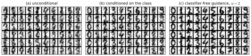
pp. 873–874 Image models use a U-net (Figure 25.3, a diagram) or a transformer for \(\beps_{\bm\theta}\), with the time step encoded by sinusoidal features and fed to the residual blocks. Figure 25.4 shows a small VDM trained on EMNIST; my stand-in below uses the 8 × 8 digits and an MLP.
25.3 Score-based generative models (SGMs)
p. 874 Instead of a scalar energy whose gradient is the score (Chapter 24 of the book), a score-based generative model learns the score \(\bm s_{\bm\theta}(\bx)\approx\nabla_{\bx}\log p_{\mathcal D}(\bx)\) directly, by basic (implicit) score matching, sliced score matching or denoising score matching (Song and Ermon, 2019, 2020; Song et al., 2021). Implicit score matching minimises \(\E_{p_{\mathcal D}}\big[\tfrac12\|\bm s_{\bm\theta}(\bx)\|^2+\Tr\nabla_{\bx}\bm s_{\bm\theta}(\bx)\big]\), which equals the Fisher divergence \(\frac12\E\|\bm s_{\bm\theta}-\nabla\log p_{\mathcal D}\|^2\) up to a constant (Result 20.10 of the deep-learning course). Samples are then drawn by Langevin dynamics, \(\bx\leftarrow\bx+\frac{\eta}{2}\bm s_{\bm\theta}(\bx)+\sqrt\eta\,\bm z\) (Section 12.5.6).
25.3.1 Example
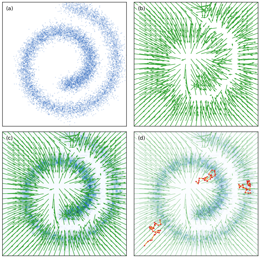
pp. 874–875 Figure 25.5 fits an MLP with two hidden layers of 128 units to the Swiss roll by basic score matching. The field points into the roll from outside and away from the empty region between the arms.
25.3.2 Adding noise at multiple scales
pp. 874–876 Score matching fails where the data have little mass. If \(p_{\mathcal D}=\pi p_0+(1-\pi)p_1\) with disjoint supports \(S_0,S_1\), then \[ \nabla_{\bx}\log p_{\mathcal D}(\bx)=\begin{cases}\nabla_{\bx}\log p_0(\bx),&\bx\in S_0,\\ \nabla_{\bx}\log p_1(\bx),&\bx\in S_1,\end{cases} \tag{25.30} \] which does not involve \(\pi\), and Langevin chains cannot cross between the modes. The remedy is to perturb the data with noise of several scales, \(q_\sigma(\tilde\bx\given\bx)=\N(\tilde\bx\given\bx,\sigma^2\bI)\), \(q_\sigma(\tilde\bx)=\int p_{\mathcal D}(\bx)q_\sigma(\tilde\bx\given\bx)\d\bx\) (25.31–25.32): large noise connects the modes, small noise is faithful to the data, and annealed Langevin dynamics or a diffusion sampler moves from the largest to the smallest scale. One noise conditional score network \(\bm s_{\bm\theta}(\bx,\sigma)\) is trained by denoising score matching at every scale, \[ L(\bm\theta;\sigma)=\frac12\E_{p_{\mathcal D}(\bx)}\E_{\tilde\bx\sim\N(\bx,\sigma^2\bI)}\Big\|\bm s_{\bm\theta}(\tilde\bx,\sigma)+\frac{\tilde\bx-\bx}{\sigma^2}\Big\|^2,\qquad L(\bm\theta;\sigma_{1:T})=\sum_t\lambda_tL(\bm\theta;\sigma_t), \tag{25.33-25.36} \] using \(\nabla_{\tilde\bx}\log\N(\tilde\bx\given\bx,\sigma^2\bI)=(\bx-\tilde\bx)/\sigma^2\) (25.35). Denoising score matching equals explicit score matching on \(q_\sigma\) up to a constant (Result 20.11 of the deep-learning course; confirmed numerically here with a linear score model).
Filling the gap 25.5: score matching cannot see mixture weights, and Langevin chains keep their starting split pp. 874–876, (25.30)
Proof
(25.30). On the interior of \(S_0\) (outside \(S_1\)), \(p_{\mathcal D}=\pi p_0\), so \(\log p_{\mathcal D}=\log\pi+\log p_0\) and the constant disappears under the gradient; likewise on \(S_1\). So the Fisher divergence \(\frac12\E_{p_{\mathcal D}}\|\bm s-\nabla\log p_{\mathcal D}\|^2\) is minimised by the same \(\bm s\) for every \(\pi\in(0,1)\), and the score-matching objective cannot identify \(\pi\). For overlapping but well-separated modes (two Gaussians at distance 3 with standard deviation 0.2) the score near each mode agrees for weights 0.8/0.2 and 0.3/0.7 to machine precision.
Langevin. Langevin dynamics has the right stationary distribution, but its mixing time between modes grows like \(\exp(\Delta U)\), where \(\Delta U\) is the height of the barrier \(-\log p_{\mathcal D}\) between them (Kramers' law); with disjoint supports it never crosses. Over any practical number of steps the share of chains in each mode is therefore the share that started in its basin, not \(\pi\). Gap 20.6 of the deep-learning course shows how annealing over noise levels restores the weights: at a large noise level the modes overlap, chains move freely and settle in proportion to the weights, and the decreasing noise levels keep that proportion. In the demonstration below, 1 000 Langevin steps with the exact data score put 49.9% of the chains in a mode of weight 0.2; the same steps annealed over 10 levels give 24.2%, and the ancestral diffusion sampler 19.6%. \(\square\)
25.3.3 Equivalence to DDPM
pp. 876–877 Writing \(\bx_t=\bx_0+\sigma_t\beps\) and \(\bm s_{\bm\theta}(\bx_t,t)=-\beps_{\bm\theta}(\bx_t,t)/\sigma_t\), the multiscale loss (25.37) becomes \(\E\big[\frac{\lambda_t}{\sigma_t^2}\|\beps-\beps_{\bm\theta}(\bx_t,t)\|^2\big]\) (25.38), and \(\lambda_t=\sigma_t^2\) gives \(L_{\rm simple}\).
Filling the gap 25.6: score-based models and DDPMs are the same model, in either parameterisation pp. 876–877, (25.37)–(25.38)
Proof
Variance exploding (the book's version). With \(\bx_t=\bx_0+\sigma_t\beps\), \((\bx_t-\bx_0)/\sigma_t^2=\beps/\sigma_t\), so \(\bm s_{\bm\theta}+(\bx_t-\bx_0)/\sigma_t^2=(\beps-\beps_{\bm\theta})/\sigma_t\), whose squared norm is \(\|\beps-\beps_{\bm\theta}\|^2/\sigma_t^2\), which gives (25.38).
Variance preserving (the DDPM's). \(L_{\rm simple}\) belongs to \(\bx_t=\sqrt{\ab_t}\bx_0+\sqrt{1-\ab_t}\beps\), not to \(\bx_0+\sigma_t\beps\). There the conditional score is \(\nabla\log q(\bx_t\given\bx_0)=-(\bx_t-\sqrt{\ab_t}\bx_0)/(1-\ab_t)=-\beps/\sqrt{1-\ab_t}\); with \(\bm s_{\bm\theta}=-\beps_{\bm\theta}/\sqrt{1-\ab_t}\), denoising score matching with weight \(\lambda_t\) is \(\E\big[\frac{\lambda_t}{1-\ab_t}\|\beps-\beps_{\bm\theta}\|^2\big]\), and \(\lambda_t=1-\ab_t\) gives \(L_{\rm simple}\). The two processes differ only by the rescaling \(\bx_t^{\rm VE}=\bx_t^{\rm VP}/\sqrt{\ab_t}\) with \(\sigma_t^2=(1-\ab_t)/\ab_t\), so either way the noise predictor is a rescaled score: \(\beps^*(\bx_t,t)=\E[\beps\given\bx_t]=-\sqrt{1-\ab_t}\,\nabla\log q_t(\bx_t)\) (confirmed by quadrature for a mixture, together with Tweedie's formula \(\E[\bx_0\given\bx_t]=(\bx_t+(1-\ab_t)\nabla\log q_t)/\sqrt{\ab_t}\), which gives every sampler below its \(\hat\bx_0\)). \(\square\)
25.4 Continuous time models using differential equations
p. 877 Letting the number of steps (or noise levels) go to infinity turns the chain into a stochastic differential equation. The mathematics is harder, but the large literature on ODE and SDE solvers becomes available for sampling.
25.4.1 Forwards diffusion SDE
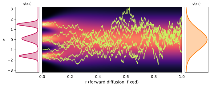
pp. 877–878 With \(\beta_t=\beta(t)\Delta t\), a first-order expansion of \(\sqrt{1-\beta(t)\Delta t}\) gives \(\bx_t-\bx_{t-1}\approx-\frac12\beta(t)\bx_{t-1}\Delta t+\sqrt{\beta(t)\Delta t}\,\N(\bm0,\bI)\) (25.39–25.41) and, in the limit, the variance-preserving SDE \[ \d\bx=-\tfrac12\beta(t)\bx\,\d t+\sqrt{\beta(t)}\,\d\bm w, \tag{25.42, 25.45} \] an instance of \(\d\bx=\bm f(\bx,t)\d t+g(t)\d\bm w\) (25.43) with drift \(\bm f\) and diffusion coefficient \(g\). Paths are simulated by Euler-Maruyama, \(\bx(t+\Delta t)=\bx(t)+\bm f\Delta t+g\sqrt{\Delta t}\,\N(\bm0,\bI)\) (25.44). The score-based (SMLD) models correspond instead to the variance-exploding SDE \(\d\bx=\sqrt{\d[\sigma(t)^2]/\d t}\,\d\bm w\) (25.46), with no drift.
Filling the gap 25.7: the marginals of the VP and VE SDEs, and the discrete-to-continuous limit pp. 877–878, (25.42)–(25.46)
Proof
VP. Let \(B(t)=\int_0^t\beta\). By Itô's formula \(\d\big(e^{B(t)/2}\bx\big)=e^{B/2}\big(\tfrac12\beta\bx\,\d t+\d\bx\big)=e^{B/2}\sqrt{\beta}\,\d\bm w\), so \(\bx(t)=e^{-B(t)/2}\bx(0)+\int_0^te^{-(B(t)-B(s))/2}\sqrt{\beta(s)}\,\d\bm w(s)\). The stochastic integral is Gaussian with mean zero and, by the Itô isometry, covariance \(\int_0^te^{-(B(t)-B(s))}\beta(s)\,\d s\,\bI=\big[e^{-(B(t)-B(s))}\big]_{s=0}^{s=t}\bI=(1-e^{-B(t)})\bI\). Hence \(q(\bx_t\given\bx_0)=\N(e^{-B(t)/2}\bx_0,(1-e^{-B(t)})\bI)\): the continuous \(\ab(t)=e^{-B(t)}\), and if \(\cov\bx_0=\bI\) then \(\cov\bx_t=\bI\) for all \(t\) ("variance preserving"). Simulated moments agree to two decimals.
The limit. With \(\beta_i=\beta(i/T)/T\) (that is, \(\beta(t/T)=T\beta_t\) as in the book), \(\log\ab_T=\sum_i\log(1-\beta(i/T)/T)=-\frac1T\sum_i\beta(i/T)+O(1/T)\to-\int_0^1\beta\), since \(\log(1-x)=-x+O(x^2)\) and the Riemann sum converges. So the DDPM chain with \(\beta_t\) linear from \(10^{-4}\) to 0.02 and \(T=1000\) is the VP SDE with \(\beta(t)\) linear from 0.1 to 20 (Figure 25.x1; largest difference in \(\ab\) below 0.003).
VE. With zero drift, \(\bx(t)=\bx(0)+\int_0^tg\,\d\bm w\) and the variance is \(\int_0^tg(s)^2\d s=\int_0^t\frac{\d\sigma^2}{\d s}\d s=\sigma(t)^2-\sigma(0)^2\): the noise level is \(\sigma(t)\) (when \(\sigma(0)\approx0\)) and the variance grows without bound. \(\square\)
25.4.2 Forwards diffusion ODE
pp. 878–879 The deterministic probability-flow ODE \[ \d\bx=\Big[\bm f(\bx,t)-\tfrac12g(t)^2\nabla_{\bx}\log p_t(\bx)\Big]\d t=\bm h(\bx,t)\,\d t \tag{25.47} \] moves a random initial point so that its marginals are the same \(p_t\) as those of the SDE (Song et al., 2021); \(\bx(t)=\bx(0)+\int_0^t\bm h\,\d\tau\) (25.48) can be computed with any ODE solver.
25.4.3 Reverse diffusion SDE
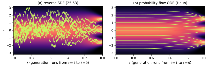
pp. 879–880 Anderson (1982) showed that the forward SDE (25.43) has the reverse-time SDE \[ \d\bx=\big[\bm f(\bx,t)-g(t)^2\nabla_{\bx}\log q_t(\bx)\big]\d t+g(t)\,\d\bar{\bm w}, \tag{25.49} \] run from \(t=1\) to 0, where \(\d t\lt0\) and \(\bar{\bm w}\) is a Wiener process in reversed time. For the DDPM it is \(\d\bx=[-\frac12\beta\bx-\beta\nabla\log q_t]\d t+\sqrt\beta\,\d\bar{\bm w}\) (25.50); with the learned score \(\bm s_{\bm\theta}\approx\nabla\log q_t\) (25.51), \(\d\bx=-\frac12\beta(t)[\bx+2\bm s_{\bm\theta}]\d t+\sqrt{\beta(t)}\d\bar{\bm w}\) (25.52), whose Euler-Maruyama step backwards in time is \[ \bx_{t-\Delta t}=\bx_t+\tfrac12\beta(t)\big[\bx_t+2\bm s_{\bm\theta}(\bx_t,t)\big]\Delta t+\sqrt{\beta(t)\Delta t}\,\N(\bm0,\bI). \tag{25.53} \]
Filling the gap 25.8: the probability-flow ODE and the reverse SDE from the Fokker-Planck equation pp. 878–880, (25.47), (25.49), (25.53)
Proof
Fokker-Planck. Let \(p_t\) be the density of \(\bx(t)\) for \(\d\bx=\bm f\d t+g\,\d\bm w\), assumed smooth and decaying fast enough to integrate by parts. For a smooth compactly supported test function \(\varphi\), Itô's formula gives \(\d\varphi(\bx)=\big(\nabla\varphi\cdot\bm f+\tfrac12g^2\Delta\varphi\big)\d t+g\nabla\varphi\cdot\d\bm w\); taking expectations (the martingale term has mean zero) and integrating by parts, \[ \frac{\d}{\d t}\int\varphi\,p_t=\int\big(\nabla\varphi\cdot\bm f+\tfrac12g^2\Delta\varphi\big)p_t=\int\varphi\Big[-\nabla\cdot(\bm fp_t)+\tfrac12g^2\Delta p_t\Big]. \] As this holds for every \(\varphi\), \(\partial_tp_t=-\nabla\cdot(\bm fp_t)+\frac12g^2\Delta p_t\).
The ODE (25.47). Since \(\Delta p=\nabla\cdot\nabla p=\nabla\cdot(p\nabla\log p)\), the Fokker-Planck equation is \(\partial_tp_t=-\nabla\cdot\big[(\bm f-\frac12g^2\nabla\log p_t)p_t\big]=-\nabla\cdot(\bm hp_t)\). That is the continuity (Liouville) equation of the ODE \(\dot\bx=\bm h(\bx,t)\): for an ODE, \(\frac{\d}{\d t}\int\varphi p_t=\int\nabla\varphi\cdot\bm h\,p_t\), which integrates by parts to the same right-hand side. Both equations start from the same \(p_0\); under uniqueness of solutions of the continuity equation (true when \(\bm h\) is locally Lipschitz with linear growth), the ODE has the marginals \(p_t\). Confirmed on a grid for a mixture (both sides agree to \(10^{-3}\) relative) and by pushing 20 000 data draws through the ODE (Kolmogorov-Smirnov distance 0.006 to the exact \(q_{0.5}\)).
The reverse SDE (25.49). Let \(\tau=1-t\) and \(\hat p_\tau=p_{1-\tau}\). Then \(\partial_\tau\hat p=-\partial_tp=\nabla\cdot(\bm fp)-\frac12g^2\Delta p\). We look for a forward-in-\(\tau\) SDE \(\d\bm y=\bm b\,\d\tau+g\,\d\bm w\) with this marginal; its Fokker-Planck equation is \(\partial_\tau\hat p=-\nabla\cdot(\bm b\hat p)+\frac12g^2\Delta\hat p\). Matching, \(\nabla\cdot(\bm b\hat p)=-\nabla\cdot(\bm f\hat p)+g^2\Delta\hat p=\nabla\cdot\big[(-\bm f+g^2\nabla\log\hat p)\hat p\big]\), which holds with \(\bm b=-\bm f+g^2\nabla\log p_{1-\tau}\). In the original clock (\(\d t=-\d\tau\)) this is \(\d\bx=[\bm f-g^2\nabla\log p_t]\d t+g\,\d\bar{\bm w}\), which is (25.49). (Anderson proves more: the reversed process has the same path law, not only the same marginals; for sampling, the marginals are what matters.) More generally, for any \(\lambda\ge0\), \(\d\bx=[\bm f-\frac{1+\lambda^2}{2}g^2\nabla\log p_t]\d t+\lambda g\,\d\bar{\bm w}\) has the same marginals: \(\lambda=0\) is the ODE, \(\lambda=1\) the reverse SDE.
(25.53). Integrating (25.52) from \(t\) to \(t-\Delta t\) with the coefficients frozen at \(t\): the drift contributes \(-\frac12\beta[\bx+2\bm s]\cdot(-\Delta t)\) and the noise \(\sqrt{\beta\Delta t}\,\N(\bm0,\bI)\). Run with the exact score of a three-component mixture (1 000 steps), it recovers the mixture weights to within 0.015. \(\square\)
25.4.4 Reverse diffusion ODE
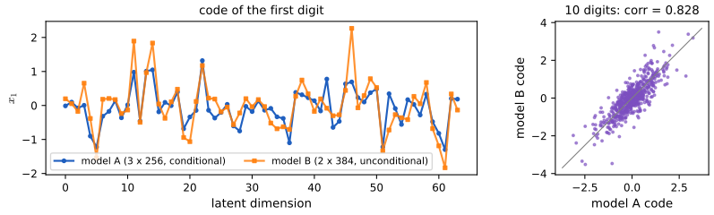
p. 880 The probability-flow ODE of the reverse process is \(\d\bx=[\bm f-\frac12g^2\bm s_{\bm\theta}]\d t\) (25.54); for the DDPM, \(\d\bx=-\frac12\beta(t)[\bx+\bm s_{\bm\theta}(\bx,t)]\d t\) (25.55), with the Euler step \(\bx_{t-\Delta t}=\bx_t+\frac12\beta(t)[\bx_t+\bm s_{\bm\theta}]\Delta t\) (25.56). Higher-order solvers such as Heun's do better (Karras et al., 2022). The ODE is a continuous normalizing flow (the book's Section 23.2.6), so the exact likelihood is available; and since the map from data to latent is fixed by the score, two different networks that both learn the score well give the same latent code for a data point (identifiability, Figure 25.8), which also allows interpolation in latent space (Section 20.3.5).
Filling the gap 25.10: the exact likelihood of the probability-flow ODE, and why its codes are identifiable p. 880
Proof
Instantaneous change of variables. Let \(\dot\bx=\bm h(\bx,t)\) have marginals \(p_t\) (gap 25.8), so \(\partial_tp_t+\nabla\cdot(p_t\bm h)=0\). Along a trajectory, \(\frac{\d}{\d t}\log p_t(\bx(t))=\frac{\partial_tp_t+\nabla p_t\cdot\bm h}{p_t}=\frac{-p_t\nabla\cdot\bm h}{p_t}=-\div\bm h(\bx(t),t)\). Integrating, \(\log p_0(\bx(0))=\log p_1(\bx(1))+\int_0^1\div\bm h(\bx(t),t)\,\d t\): run the ODE forwards from a data point to its code \(\bx(1)\), evaluate the Gaussian prior there, and add the integrated divergence (estimated by Hutchinson's trace estimator in high dimension). Result 20.13 of the deep-learning course gives the same statement.
Identifiability. The encoder \(\bx(0)\mapsto\bx(1)\) is the flow map of an ODE whose vector field \(-\frac12\beta(\bx+\nabla\log q_t)\) is determined by the data distribution and the fixed schedule alone. Two networks with the same score therefore define the same map, whatever their architectures; errors in the learned scores perturb the code by an amount controlled by Grönwall's inequality (the score error times \(e^{\int\mathrm{Lip}(\bm h)}\)). Figure 25.8 checks this with two networks trained on the digits: their codes have correlation 0.83, against about 0 for unrelated codes. \(\square\)
25.4.5 Comparison of the SDE and ODE approach
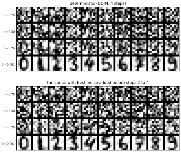
p. 881 The reverse SDE splits into the probability-flow ODE plus a Langevin diffusion: \[ \d\bx_t=\underbrace{-\tfrac12\beta(t)[\bx_t+\bm s_{\bm\theta}(\bx_t,t)]\d t}_{\text{probability-flow ODE}}\ \underbrace{-\tfrac12\beta(t)\bm s_{\bm\theta}(\bx_t,t)\d t+\sqrt{\beta(t)}\d\bar{\bm w}_t}_{\text{Langevin diffusion}}. \tag{25.57} \] The injected noise corrects errors made by integrating the ODE part, so SDE samples often look better, while the ODE can take fewer steps. Karras et al. (2022) alternate a deterministic solver step with a small amount of added noise (Figure 25.9).
Filling the gap 25.9: the Langevin part of (25.57) leaves every \(q_t\) invariant, which is why it corrects errors p. 881, (25.57)
Proof
The split. The two drifts add to \(-\frac12\beta\bx-\beta\bm s\), the drift of (25.52), and the noise is that of (25.52), so (25.57) is an exact rewriting.
Invariance. Freeze \(t\) and consider the Langevin part alone, in the direction of generation (reversed time \(\tau\)): \(\d\bm y=\frac12\beta\nabla\log q_t(\bm y)\d\tau+\sqrt\beta\,\d\bm w\). Its Fokker-Planck operator applied to \(q_t\) is \(-\nabla\cdot(\frac12\beta q_t\nabla\log q_t)+\frac12\beta\Delta q_t=-\frac12\beta\Delta q_t+\frac12\beta\Delta q_t=0\): \(q_t\) is stationary. So the Langevin term does not move the marginals when they are right, and when the current distribution has drifted away from \(q_t\) (because of discretisation or score error) it contracts it back towards \(q_t\) at the rate of a Langevin sampler. The ODE part transports \(q_t\) to \(q_{t-\d t}\) on its own. Checked on a grid: the Langevin flux vanishes to \(10^{-3}\) of the size of \(\partial_tq_t\). \(\square\)
25.4.6 Example
p. 881 The book fits a small score model to MNIST by denoising score matching and samples by solving the probability-flow ODE; scaled up, the same recipe produces the faces of Figure 25.10 (Song et al., 2021, trained on CelebA-HQ at 256 × 256, not reproduced). The digit model of Figures 25.4, 25.8 and 25.9 is the small-scale version of this example.
25.4.7 Flow matching
pp. 881–882 Seen as a continuous normalizing flow, a diffusion model need not involve Gaussian noise at all. Flow matching (Albergo and Vanden-Eijnden, 2023; Lipman et al., 2023; Liu, Gong and Liu, 2023) learns a velocity field \(\bm v_{\bm\theta}(\bx_t,t)\approx\frac{\d}{\d t}\bx_t\) for an interpolant \(\bx_t=I_t(\bx_0,\bx_1)=\alpha_t\bx_0+\beta_t\bx_1\) between a source \(\bx_0\sim p_0\) and a target \(\bx_1\sim p_1\) (e.g. \(\alpha_t=1-t\), \(\beta_t=t\)), by regressing on \(\frac{\d}{\d t}I_t=\bx_1-\bx_0\); samples are \(\bx_1=\bx_0+\int_0^1\bm v_{\bm\theta}(\bx_t,t)\d t\). The source may be non-Gaussian, the likelihood is exact, and couplings chosen by optimal transport (Section 6.8) straighten the paths and speed up integration.
Filling the gap 25.11: why regressing on \(\bx_1-\bx_0\) learns a flow with the right marginals, and its likelihood p. 882
Proof
The marginal velocity. Let \((\bx_0,\bx_1)\) have any coupling with marginals \(p_0,p_1\), \(\bx_t=(1-t)\bx_0+t\bx_1\) with law \(p_t\), and \(\bm u(\bx,t)=\E[\bx_1-\bx_0\given\bx_t=\bx]\). For a test function \(\varphi\), \(\frac{\d}{\d t}\E\varphi(\bx_t)=\E[\nabla\varphi(\bx_t)\cdot(\bx_1-\bx_0)]=\E[\nabla\varphi(\bx_t)\cdot\bm u(\bx_t,t)]\) by the tower property. So \(p_t\) solves the continuity equation \(\partial_tp_t+\nabla\cdot(p_t\bm u)=0\), and (under uniqueness, gap 25.8) the ODE \(\dot\bx=\bm u(\bx,t)\) started from \(p_0\) has marginals \(p_t\), ending at \(p_1\).
Conditional regression is enough. For any \(\bm v\), expand \(\E\|\bm v(\bx_t,t)-(\bx_1-\bx_0)\|^2=\E\|\bm v-\bm u\|^2+\E\|\bm u-(\bx_1-\bx_0)\|^2+2\E[(\bm v-\bm u)\cdot(\bm u-(\bx_1-\bx_0))]\). The cross term vanishes by conditioning on \(\bx_t\) (\(\bm v-\bm u\) is a function of \(\bx_t\) and \(\E[\bm u-(\bx_1-\bx_0)\given\bx_t]=\bm 0\)). So the tractable conditional loss equals the intractable marginal loss \(\E\|\bm v-\bm u\|^2\) plus a constant: same minimiser, same gradients. Confirmed by Monte Carlo with the exact \(\bm u\) of a Gaussian source and a mixture target.
Link with diffusion. With an independent Gaussian source, \(\bx_t=t\bx_1+(1-t)\bx_0\) is a noised data point with \(\alpha=t\), \(\sigma=1-t\); Tweedie's formula gives \(\E[\bx_0\given\bx_t]=-(1-t)\nabla\log p_t\) and \(\E[\bx_1\given\bx_t]=(\bx_t+(1-t)^2\nabla\log p_t)/t\), so \(\bm u(\bx,t)=\big(\bx+(1-t)\nabla\log p_t(\bx)\big)/t\): flow matching with a Gaussian source is a probability-flow ODE in another time parameterisation (confirmed to \(10^{-9}\)).
Likelihood. By gap 25.10, \(\log p_1(\bx_1)=\log p_0(\bx_0)-\int_0^1\div\bm v(\bx_t,t)\,\d t\) along the trajectory from \(\bx_0\) to \(\bx_1\). The book writes \(p_1(\bx)=p_0(\bx)\exp(\cdots)\); the source density must be evaluated at the starting point \(\bx_0\) of the trajectory that ends at \(\bx\), not at \(\bx\). Integrating the exact \(\bm u\) and its divergence from 20 000 normal draws reproduces the target log-density to \(2\times10^{-5}\) and its mixture weights to 0.002. \(\square\)
25.5 Speeding up diffusion models
p. 882 Sampling needs many small steps; naive large steps are much worse. Four remedies follow.
25.5.1 DDIM sampler
pp. 882–883 The denoising diffusion implicit model (Song, Meng and Ermon, 2021) uses a non-Markovian forward process that conditions on \(\bx_0\) at every step, \[ q(\bx_{t-1}\given\bx_t,\bx_0)=\N\Big(\sqrt{\ab_{t-1}}\bx_0+\sqrt{1-\ab_{t-1}-\tilde\sigma_t^2}\,\frac{\bx_t-\sqrt{\ab_t}\bx_0}{\sqrt{1-\ab_t}},\ \tilde\sigma_t^2\bI\Big), \tag{25.58} \] and the reverse process plugs in the prediction \(\hat\bx_0=\hat\bx_{\bm\theta}(\bx_t,t)\) (25.59). With \(\tilde\sigma_t=0\) generation is deterministic given \(\bx_T\). The weighted bound of this model is again \(L_{\rm simple}\), so DDIM can be used with a network trained as a DDPM, and it can skip steps.
Filling the gap 25.12: DDIM keeps the DDPM marginals for every \(\tilde\sigma_t\), contains the DDPM, and is an exact step of a rescaled ODE pp. 882–883, (25.58)–(25.59)
Proof
Marginals. Suppose \(q(\bx_t\given\bx_0)=\N(\sqrt{\ab_t}\bx_0,(1-\ab_t)\bI)\) and write \(\bx_t=\sqrt{\ab_t}\bx_0+\sqrt{1-\ab_t}\beps\). Then the fraction in (25.58) is \(\beps\), and a draw from (25.58) is \(\bx_{t-1}=\sqrt{\ab_{t-1}}\bx_0+\sqrt{1-\ab_{t-1}-\tilde\sigma_t^2}\,\beps+\tilde\sigma_t\beps'\) with \(\beps'\) independent: Gaussian with mean \(\sqrt{\ab_{t-1}}\bx_0\) and covariance \((1-\ab_{t-1}-\tilde\sigma_t^2+\tilde\sigma_t^2)\bI=(1-\ab_{t-1})\bI\). By induction downwards from \(t=T\), all the marginals \(q(\bx_t\given\bx_0)\) are those of the DDPM, for any choice \(0\le\tilde\sigma_t^2\le1-\ab_{t-1}\). Each KL term of the bound then compares two Gaussians with the same covariance whose means differ by \(\big(\sqrt{\ab_{t-1}}-\sqrt{1-\ab_{t-1}-\tilde\sigma_t^2}\sqrt{\ab_t/(1-\ab_t)}\big)(\bx_0-\hat\bx_0)\), a weighted \(\|\bx_0-\hat\bx_0\|^2\), equivalently a weighted \(\|\beps-\hat\beps\|^2\): the same family of losses as \(L_{\rm simple}\).
DDPM as a special case. Take \(\tilde\sigma_t^2=\bt_t\). Then \(1-\ab_{t-1}-\bt_t=(1-\ab_{t-1})\frac{1-\ab_t-\beta_t}{1-\ab_t}=\frac{\alpha_t(1-\ab_{t-1})^2}{1-\ab_t}\) (because \(1-\beta_t-\ab_t=\alpha_t(1-\ab_{t-1})\)), so the coefficient of \(\bx_t\) in (25.58) is \(\frac{\sqrt{\alpha_t}(1-\ab_{t-1})}{1-\ab_t}\) and that of \(\bx_0\) is \(\sqrt{\ab_{t-1}}-\frac{\sqrt{\alpha_t}(1-\ab_{t-1})\sqrt{\ab_t}}{1-\ab_t}=\frac{\sqrt{\ab_{t-1}}\beta_t}{1-\ab_t}\): exactly (25.7) and (25.8).
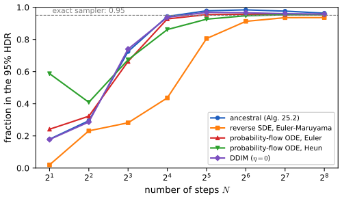
Deterministic DDIM as an ODE step. With \(\tilde\sigma=0\) and continuous-time notation \(\bx_t=\alpha_t\bx_0+\sigma_t\beps\), the step to \(s\lt t\) is \(\bx_s=\alpha_s\hat\bx_0+\sigma_s\hat\beps\) with \(\hat\beps=(\bx_t-\alpha_t\hat\bx_0)/\sigma_t\). In the variables \(\bm y=\bx/\alpha\) and \(\rho=\sigma/\alpha\) this reads \(\bm y_s=\bm y_t+(\rho_s-\rho_t)\hat\beps(\bx_t)\): an Euler step of \(\d\bm y/\d\rho=\hat\beps\), which is the probability-flow ODE rewritten in \((\bm y,\rho)\), and it is exact whenever \(\hat\beps\) (equivalently \(\hat\bx_0\)) is constant along the step. This explains why DDIM tolerates large steps much better than Euler in \(t\) (75% of samples in the 95% region with 8 steps, against 66% for Euler, in the demonstration; gap 20.4 of the deep-learning course discusses DDIM from the sampling side). \(\square\)
25.5.2 Non-Gaussian decoder networks
p. 883 If the reverse process takes large steps, the true \(q(\bx_{t-\Delta}\given\bx_t)\) becomes multimodal and a Gaussian decoder cannot fit it (Figure 25.11). Gao et al. (2021) model the step with an energy-based model (needing MCMC), Xiao, Kreis and Vahdat (2022) with a conditional GAN (Chapter 26), which keeps sampling one network pass per step and needs only a few steps.
25.5.3 Distillation
pp. 883–884 Progressive distillation (Salimans and Ho, 2022) trains a student to do in one DDIM step what the teacher does in two, then makes the student the next teacher and halves the number of steps again; high-quality samples need as few as 4 steps. Algorithm 25.3 is standard training with the clean data as target, \(\bz_t=\alpha_t\bx+\sigma_t\beps\) and loss \(w(\lambda_t)\|\bx-\hat\bx_{\bm\theta}(\bz_t)\|^2\), \(\lambda_t=\log(\alpha_t^2/\sigma_t^2)\). Algorithm 25.4 replaces the target by the teacher-derived \(\tilde\bx\) below.
Algorithm 25.4: progressive distillation
- Start with a trained teacher \(\hat\bx_{\bm\eta}\) and \(N\) sampling steps. For each of \(K\) rounds: initialise the student \(\bm\theta\leftarrow\bm\eta\).
- Repeat: draw \(\bx\sim\mathcal D\), \(t=i/N\) with \(i\) uniform in \(\{1,\dots,N\}\), \(\beps\), and set \(\bz_t=\alpha_t\bx+\sigma_t\beps\), \(t'=t-0.5/N\), \(t''=t-1/N\).
- Two teacher DDIM steps: \(\bz_{t'}=\alpha_{t'}\hat\bx_{\bm\eta}(\bz_t)+\frac{\sigma_{t'}}{\sigma_t}(\bz_t-\alpha_t\hat\bx_{\bm\eta}(\bz_t))\), and the same from \(\bz_{t'}\) to \(\bz_{t''}\).
- Target \(\tilde\bx=\dfrac{\bz_{t''}-(\sigma_{t''}/\sigma_t)\bz_t}{\alpha_{t''}-(\sigma_{t''}/\sigma_t)\alpha_t}\); gradient step on \(w(\lambda_t)\|\tilde\bx-\hat\bx_{\bm\theta}(\bz_t)\|^2\).
- After convergence: \(\bm\eta\leftarrow\bm\theta\) (the student becomes the teacher), \(N\leftarrow N/2\).
Filling the gap 25.13: where the distillation target comes from p. 884, Algorithm 25.4, lines 9–11
Proof
A deterministic DDIM step from \((\bz_t,t)\) to \(s\) with prediction \(\hat\bx\) is \(\bz_s=\alpha_s\hat\bx+\sigma_s\hat\beps\) with \(\hat\beps=(\bz_t-\alpha_t\hat\bx)/\sigma_t\), i.e. \(\bz_s=\alpha_s\hat\bx+\frac{\sigma_s}{\sigma_t}(\bz_t-\alpha_t\hat\bx)\) (gap 25.12): lines 9 and 10 are two such steps of the teacher. The student must land on the same point \(\bz_{t''}\) in one step from \(\bz_t\), i.e. its prediction \(\tilde\bx\) must solve \(\alpha_{t''}\tilde\bx+\frac{\sigma_{t''}}{\sigma_t}(\bz_t-\alpha_t\tilde\bx)=\bz_{t''}\). This is linear in \(\tilde\bx\): \(\tilde\bx\big(\alpha_{t''}-\frac{\sigma_{t''}}{\sigma_t}\alpha_t\big)=\bz_{t''}-\frac{\sigma_{t''}}{\sigma_t}\bz_t\), which is line 11. The denominator is \(\alpha_{t''}\sigma_t^{-1}\big(\sigma_t-\sigma_{t''}\alpha_t/\alpha_{t''}\big)\), which vanishes only if \(\alpha_t/\sigma_t=\alpha_{t''}/\sigma_{t''}\), impossible for a strictly monotone SNR; so the target is always defined. Confirmed numerically: one DDIM step with \(\tilde\bx\) reproduces the teacher's two-step result to \(10^{-12}\). \(\square\)
25.5.4 Latent space diffusion
pp. 884–885 A latent diffusion model (Rombach et al., 2022) first trains an autoencoder (a VAE with a perceptual loss) and then a diffusion model on its codes (Figure 25.13, a diagram); it is the basis of Stable Diffusion. The latent score-based model of Vahdat, Kreis and Kautz (2021) trains a hierarchical VAE and the diffusion prior jointly. Working in a continuous latent space also lets diffusion handle text, graphs and other discrete data; conversely, a diffusion model can post-process the blurry samples of a VAE.
25.6 Conditional generation
p. 885 To generate given side information \(c\) (a class label, a text prompt, another image), there are three approaches.
25.6.1 Conditional diffusion model
p. 885 Train on pairs \((c,\bx)\) to maximise the conditional likelihood \(p(\bx\given c)\): a label is embedded and added to the features or used to modulate group normalisation; an image is concatenated as extra channels; a text prompt is embedded and enters through cross-attention.
25.6.2 Classifier guidance
p. 886 Classifier guidance (Dhariwal and Nichol, 2021) uses a separately trained classifier \(p_{\bm\phi}(c\given\bx)\): by Bayes' rule \(\log p(\bx\given c)=\log p(c\given\bx)+\log p(\bx)-\log p(c)\) (25.60), so \[ \nabla_{\bx}\log p(\bx\given c)=\nabla_{\bx}\log p(\bx)+\nabla_{\bx}\log p(c\given\bx),\qquad \nabla_{\bx}\log p_w(\bx\given c)=\nabla_{\bx}\log p(\bx)+w\nabla_{\bx}\log p(c\given\bx), \tag{25.61-25.62} \] with \(w>1\) amplifying the label. In the ancestral sampler this is implemented by shifting the mean: \(\bx_{t-1}\sim\N(\bmu+w\bm\Sigma\bm g,\bm\Sigma)\) with \(\bm g=\nabla_{\bx_t}\log p_{\bm\phi}(c\given\bx_t)\) (25.63).
Filling the gap 25.14: the guided reverse step (25.63), and the relation between the two guidance weights p. 886, (25.61)–(25.63), (25.66)
Proof
Exact conditional step. Let the label be attached to the clean data and \(c\) be independent of the later noise: \(c\to\bx_0\to\bx_1\to\cdots\), so \(c\perp\bx_t\given\bx_{t-1}\) (the forward step adds noise that does not depend on \(c\)). Then \(q(\bx_{t-1}\given\bx_t,c)\propto q(\bx_{t-1}\given\bx_t)\,q(c\given\bx_{t-1},\bx_t)=q(\bx_{t-1}\given\bx_t)\,q(c\given\bx_{t-1})\), with normaliser \(q(c\given\bx_t)\), which does not depend on \(\bx_{t-1}\). The classifier needed is one for noisy inputs \(\bx_{t-1}\).
Gaussian approximation (25.63). With \(p_{\bm\theta}(\bx_{t-1}\given\bx_t)=\N(\bmu,\bm\Sigma)\) and the first-order expansion \(\log p_{\bm\phi}(c\given\bx_{t-1})\approx\log p_{\bm\phi}(c\given\bmu)+\bm g^\T(\bx_{t-1}-\bmu)\) (accurate when \(\bm\Sigma\) is small, i.e. small steps; \(\bm g\) is evaluated at \(\bmu\approx\bx_t\)), the product is proportional to \(\exp\big(-\frac12(\bx-\bmu)^\T\bm\Sigma^{-1}(\bx-\bmu)+\bm g^\T(\bx-\bmu)\big)\). Completing the square, \(-\frac12(\bx-\bmu-\bm\Sigma\bm g)^\T\bm\Sigma^{-1}(\bx-\bmu-\bm\Sigma\bm g)+\frac12\bm g^\T\bm\Sigma\bm g\), so the step is \(\N(\bmu+\bm\Sigma\bm g,\bm\Sigma)\); a classifier raised to the power \(w\) multiplies \(\bm g\) by \(w\). (Confirmed numerically on a grid.)
The two weights. If the classifier is exact, \(\nabla\log p(c\given\bx)=\nabla\log p(\bx\given c)-\nabla\log p(\bx)\), so (25.62) is \(w\nabla\log p(\bx\given c)+(1-w)\nabla\log p(\bx)\). Classifier-free guidance (25.66) is \((1+w')\nabla\log p(\bx\given c)-w'\nabla\log p(\bx)\). They coincide when \(w'=w-1\): classifier-guidance weight \(w\) is classifier-free weight \(w-1\), and the plain conditional model is \(w=1\), \(w'=0\). Confirmed with the exact noisy classifier of the three-class mixture to \(10^{-5}\) (finite differences). Result 20.14 of the deep-learning course states the same identity in noise-prediction form. \(\square\)
25.6.3 Classifier-free guidance
p. 886 A discriminative classifier may ignore most of the input, so following its gradient can act like an adversarial perturbation, and it must be trained on noisy inputs at every level. Classifier-free guidance (Ho and Salimans, 2021) derives the classifier from the generative model, \(\log p(c\given\bx)=\log p(\bx\given c)+\log p(c)-\log p(\bx)\) (25.64), and trains one network for both \(p(\bx\given c)\) and \(p(\bx)\) by replacing \(c\) with a null label some of the time. Then \[ \nabla_{\bx}\big[\log p(\bx\given c)+w\log p(c\given\bx)\big]=\nabla_{\bx}\big[(1+w)\log p(\bx\given c)-w\log p(\bx)\big]. \tag{25.65-25.66} \] Larger \(w\) gives individually better samples and less diversity (Figure 25.4c).
Filling the gap 25.15: the distribution guidance aims at, and why guided sampling does not reach it exactly p. 886, (25.65)–(25.66)
Proof
The tilted target. (25.66) is the score of \(\tilde p_w(\bx\given c)\propto p(\bx\given c)^{1+w}p(\bx)^{-w}=p(\bx\given c)\big[p(\bx\given c)/p(\bx)\big]^w\propto p(\bx\given c)\,p(c\given\bx)^w\), normalisable when the integral is finite. Relative to \(p(\bx\given c)\), it multiplies the density by \(p(c\given\bx)^w\): regions where other classes are also likely are suppressed, which raises the typicality of samples and lowers their diversity (practice problem 25.3 works this out for Gaussians).
Not reached exactly. A sampler that uses \((1+w)\nabla\log p_t(\bx\given c)-w\nabla\log p_t(\bx)\) at every noise level is driven by the score of \(p_t(\bx\given c)^{1+w}p_t(\bx)^{-w}\), where \(p_t\) are the noised distributions. But noising does not commute with powers: \(\big(p(\cdot\given c)^{1+w}p^{-w}\big)*\N(0,\sigma^2)\ne\big(p(\cdot\given c)*\N\big)^{1+w}\big(p*\N\big)^{-w}\) in general. So the guided reverse process is not the reverse of the forward process started from \(\tilde p_w\), and its output differs from \(\tilde p_w\) (gap 20.7 of the deep-learning course). In the demonstration, for class 1 with \(w=4\), the guided samples have spread 0.572 while the tilted target has 0.694, and the mean class probability is 1.000 against 0.991: guidance in practice concentrates more than the target it is derived from. \(\square\)
25.6.4 Generating high resolution images
pp. 886–887 Cascaded generation (Ho et al., 2022) generates a 64 × 64 image and then applies super-resolution diffusion models to reach 256 × 256 or 1024 × 1024; Imagen (Saharia et al., 2022) combines a frozen T5-XXL text encoder with such a cascade (Figure 25.14, a diagram). Conditioning on an image gives image-to-image translation (colourisation, inpainting, restoration), trainable as one multi-task conditional model (Saharia et al., 2022).
25.7 Diffusion for discrete state spaces
p. 887 For discrete data (text, segmentation labels) one can diffuse in a continuous embedding (Section 25.5.4) or define the corruption directly on the discrete states.
25.7.1 Discrete Denoising Diffusion Probabilistic Models
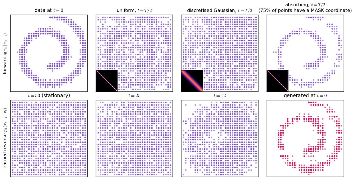
pp. 887–888 The D3PM (Austin et al., 2021), building on multinomial diffusion (Hoogeboom et al., 2021), needs three things: sampling \(q(\bx_t\given\bx_0)\) for any \(t\), a tractable \(q(\bx_{t-1}\given\bx_t,\bx_0)\) for the KL terms \(L_{t-1}(\bx_0)=\E_{q(\bx_t\given\bx_0)}\Dkl(q(\bx_{t-1}\given\bx_t,\bx_0)\|p_{\bm\theta}(\bx_{t-1}\given\bx_t))\) (25.67), and a stationary distribution for the prior, so that \(L_T=0\). Each of \(D\) independent coordinates takes one of \(K\) values, written as a one-hot row vector \(\bx\); the forward kernel is \[ q(\bx_t\given\bx_{t-1})=\Cat(\bx_t\given\bx_{t-1}\bQ_t),\qquad[\bQ_t]_{ij}=q(x_t=j\given x_{t-1}=i), \tag{25.68} \] with marginal and posterior \[ q(\bx_t\given\bx_0)=\Cat(\bx_t\given\bx_0\bar\bQ_t),\ \ \bar\bQ_t=\bQ_1\cdots\bQ_t;\qquad q(\bx_{t-1}\given\bx_t,\bx_0)=\Cat\Big(\bx_{t-1}\,\Big|\,\frac{\bx_t\bQ_t^\T\odot\bx_0\bar\bQ_{t-1}}{\bx_0\bar\bQ_t\bx_t^\T}\Big). \tag{25.69-25.70} \]
Filling the gap 25.16: the marginal (25.69) and the posterior (25.70) of a discrete chain p. 888
Proof
(25.69). By the Markov property and the law of total probability (Chapman-Kolmogorov), \(q(x_t=j\given x_0=i)=\sum_{k_1,\dots,k_{t-1}}[\bQ_1]_{ik_1}[\bQ_2]_{k_1k_2}\cdots[\bQ_t]_{k_{t-1}j}=[\bQ_1\bQ_2\cdots\bQ_t]_{ij}\), the definition of the matrix product. For a one-hot \(\bx_0=\bm e_i\), \(\bx_0\bar\bQ_t\) is row \(i\) of \(\bar\bQ_t\); for a probability vector \(\bx_0\) it is the mixture of rows.
(25.70). By Bayes' rule and the Markov property, \(q(x_{t-1}=k\given x_t=j,x_0=i)=\frac{q(x_t=j\given x_{t-1}=k)\,q(x_{t-1}=k\given x_0=i)}{q(x_t=j\given x_0=i)}=\frac{[\bQ_t]_{kj}[\bar\bQ_{t-1}]_{ik}}{[\bar\bQ_t]_{ij}}\). As a row vector over \(k\): the first factor is \((\bx_t\bQ_t^\T)_k\) (column \(j\) of \(\bQ_t\)), the second \((\bx_0\bar\bQ_{t-1})_k\), the denominator \(\bx_0\bar\bQ_t\bx_t^\T\). The numerators sum over \(k\) to \([\bar\bQ_{t-1}\bQ_t]_{ij}=[\bar\bQ_t]_{ij}\), so it is a probability vector. Because both distributions factorise over the \(D\) coordinates, the KL in (25.67) is a sum of \(D\) categorical KLs. Both formulas were confirmed against brute-force path sums for a three-state chain. \(\square\)
25.7.2 Choice of Markov transition matrices for the forward processes
pp. 889–890 The uniform kernel \(\bQ_t=(1-\beta_t)\bI+\beta_t\one\one^\T/K\) (the book writes \(\beta_t/K\) for the matrix \(\beta_t\one\one^\T/K\)) has entries \(1-\frac{K-1}{K}\beta_t\) on the diagonal and \(\beta_t/K\) elsewhere (25.71); its stationary distribution is uniform, and \[ q(\bx_t\given\bx_0)=\Cat\big(\bx_t\given\ab_t\bx_0+(1-\ab_t)/K\big),\qquad \tilde{\bm\theta}=\big[\alpha_t\bx_t+(1-\alpha_t)/K\big]\odot\big[\ab_{t-1}\bx_0+(1-\ab_{t-1})/K\big], \tag{25.72-25.74} \] with \(q(\bx_{t-1}\given\bx_t,\bx_0)=\Cat(\tilde{\bm\theta}/\sum_k\tilde\theta_k)\). The absorbing kernel moves to a MASK state \(m\) with probability \(\beta_t\): \(\bQ_t=(1-\beta_t)\bI+\beta_t\one\bm e_m^\T\) (25.75), converging to a point mass on \(m\). The discretised Gaussian kernel moves mostly to nearby levels, for ordinal data; made doubly stochastic, it also has a uniform stationary distribution.
Filling the gap 25.17: the three kernels in closed form, and their stationary distributions pp. 889–890, (25.71)–(25.75)
Proof
Uniform kernel. Let \(\bm U=\one\one^\T/K\); then \(\bm U^2=\bm U\) (\(\one^\T\one=K\)). For two such matrices, \((a\bI+(1-a)\bm U)(b\bI+(1-b)\bm U)=ab\bI+[a(1-b)+(1-a)b+(1-a)(1-b)]\bm U=ab\bI+(1-ab)\bm U\). By induction \(\bar\bQ_t=\ab_t\bI+(1-\ab_t)\bm U\), and row \(\bx_0\) of it is \(\ab_t\bx_0+(1-\ab_t)\one^\T/K\), which is (25.72). In (25.70), \(\bQ_t\) is symmetric, so \(\bx_t\bQ_t^\T=\bx_t\bQ_t=\alpha_t\bx_t+(1-\alpha_t)/K\), and \(\bx_0\bar\bQ_{t-1}=\ab_{t-1}\bx_0+(1-\ab_{t-1})/K\), which gives (25.73)–(25.74). The uniform vector \(\bm\pi\) satisfies \(\bm\pi\bQ_t=\bm\pi\) because the columns sum to 1 (doubly stochastic); since all entries are positive, Perron-Frobenius gives uniqueness and convergence, and explicitly \(\bar\bQ_t\to\bm U\) as \(\ab_t\to0\).
Absorbing kernel. Let \(\bm A=\one\bm e_m^\T\) (every row equals \(\bm e_m^\T\)); then \(\bm A^2=\one(\bm e_m^\T\one)\bm e_m^\T=\bm A\). As above, \(((1-a)\bI+a\bm A)((1-b)\bI+b\bm A)=(1-a)(1-b)\bI+(1-(1-a)(1-b))\bm A\), so \(\bar\bQ_t=\ab_t\bI+(1-\ab_t)\one\bm e_m^\T\): a token keeps its value with probability \(\ab_t\) and is MASK otherwise. Row \(m\) of \(\bQ_t\) is \(\bm e_m^\T\), so \(\bm e_m\) is stationary, and every other state reaches it, so it is the unique stationary distribution.
Discretised Gaussian. The off-diagonal entries \(\propto\exp(-4(i-j)^2/((K-1)^2\beta_t))\) are symmetric in \(i,j\), and the diagonal is set so rows sum to 1; a symmetric matrix with unit row sums has unit column sums, hence is doubly stochastic and preserves the uniform distribution. All three closed forms were confirmed against explicit matrix products. \(\square\)
25.7.3 Parameterization of the reverse process
p. 890 Rather than predicting the logits of \(p_{\bm\theta}(\bx_{t-1}\given\bx_t)\) directly, it is better to predict \(\tilde p_{\bm\theta}(\tilde\bx_0\given\bx_t)\) and combine it with the exact posterior: \[ p_{\bm\theta}(\bx_{t-1}\given\bx_t)\propto\sum_{\tilde\bx_0}q(\bx_{t-1}\given\bx_t,\tilde\bx_0)\,\tilde p_{\bm\theta}(\tilde\bx_0\given\bx_t),\qquad p_{\bm\theta}(\bx_{t-k}\given\bx_t)\propto\sum_{\tilde\bx_0}q(\bx_{t-k}\given\bx_t,\tilde\bx_0)\,\tilde p_{\bm\theta}(\tilde\bx_0\given\bx_t). \tag{25.76-25.77} \] The sum costs \(O(DK)\) per coordinate set; the model automatically respects the zeros of \(\bQ_t\), can skip \(k\) steps, and, being categorical, is multimodal already (contrast Section 25.5.2).
Filling the gap 25.18: why the \(\bx_0\)-parameterisation respects sparsity, and the \(k\)-step posterior p. 890, (25.76)–(25.77)
Proof
Sparsity. If a transition \(x_{t-1}=k\to x_t=j\) is impossible (\([\bQ_t]_{kj}=0\)), then \(q(x_{t-1}=k\given x_t=j,\tilde x_0)=0\) for every \(\tilde x_0\) by (25.70), so every term of (25.76) vanishes at \(k\), whatever the network outputs. For the absorbing kernel, for example, a non-mask token \(x_t=j\) forces \(x_{t-1}=j\) (masks never unmask in the forward direction), and a direct parameterisation would have to learn this; (25.76) gets it for free. Also, the minimiser over \(\tilde p\) of the expected cross-entropy \(\E[-\log\tilde p(\bx_0\given\bx_t)]\) is the true \(q(\bx_0\given\bx_t)\), and then (25.76) is exactly \(\sum_{\bx_0}q(\bx_{t-1}\given\bx_t,\bx_0)q(\bx_0\given\bx_t)=q(\bx_{t-1}\given\bx_t)\), the minimiser of (25.67); this is why training on the \(\bx_0\) cross-entropy (as for Figure 25.16) targets the right reverse step.
\(k\) steps. The same Bayes argument as in gap 25.16, with the \(k\)-step kernel \(\bQ_{t-k+1}\cdots\bQ_t\) in place of \(\bQ_t\), gives \(q(\bx_{t-k}\given\bx_t,\bx_0)\propto\big(\bx_t(\bQ_{t-k+1}\cdots\bQ_t)^\T\big)\odot\bx_0\bar\bQ_{t-k}\), and (25.77) is the corresponding mixture. \(\square\)
25.7.4 Noise schedules
p. 890 For the discretised Gaussian, Austin et al. increase the variance linearly; for uniform diffusion, the cosine schedule of Nichol and Dhariwal (2021); for masking, \(\beta_t=1/(T-t+1)\) (Sohl-Dickstein et al., 2015).
Filling the gap 25.19: the masking schedule unmasks linearly, and the cosine schedule as it should read p. 890
Proof
Masking. With \(\beta_s=1/(T-s+1)\), \(1-\beta_s=\frac{T-s}{T-s+1}\) and the product telescopes: \(\ab_t=\prod_{s=1}^t\frac{T-s}{T-s+1}=\frac{T-t}{T}\). So the expected fraction of unmasked tokens falls linearly from 1 to 0, and \(\ab_T=0\): \(\bx_T\) is all MASK, exactly the stationary distribution (\(L_T=0\)). From gap 25.17, a token that is MASK at time \(t\) was still unmasked at time \(t-1\) with probability \(\frac{\beta_t\ab_{t-1}}{1-\ab_t}=\frac{1}{T-t+1}\cdot\frac{(T-t+1)/T}{t/T}=\frac1t\): the reverse process unmasks each masked token with probability \(1/t\) per step, a uniformly random order (preset 3 of the demonstration shows 0.04 at \(t=25\)).
Cosine. Nichol and Dhariwal define the cumulative \(\ab_t=f(t)/f(0)\) with \(f(t)=\cos^2\big(\frac{t/T+s}{1+s}\frac\pi2\big)\), \(s=0.008\), and \(\beta_t=1-\ab_t/\ab_{t-1}\) (clipped at 0.999). The book writes the per-step \(\alpha_t=\cos\big(\frac{t/T+s}{1+s}\frac\pi2\big)\) with \(\beta_t=1-\alpha_t\). Read literally, \(\ab_t=\prod_{u\le t}\alpha_u\) collapses: for \(T=1000\), \(\ab_{200}=0.025\) and \(\ab_{300}=5\times10^{-6}\), against 0.90 and 0.79 for the intended schedule, so the signal is gone less than a third of the way through (Figure 25.x1). With the intended definition, \(\ab_{T/2}\approx0.49\) and the log-SNR falls almost linearly. \(\square\)
25.7.5 Connections to other probabilistic models for discrete sequences
pp. 890–891 With \(\bQ=\alpha\one\bm e_m^\T+\beta\one\one^\T/K+(1-\alpha-\beta)\bI\) and a single step that masks 10% of the tokens and randomises 5%, the bound reduces to the BERT objective \(L_0(\bx_0)=-\E_{q(\bx_1\given\bx_0)}\log p_{\bm\theta}(\bx_0\given\bx_1)\) (25.78). A deterministic process that masks one more token per step (masking diffusion) gives the cross-entropy of an any-order autoregressive model (Ou et al., 2024), and generative masked language models and MaskGIT (Chang et al., 2022; Figure 25.17, a diagram), which unmask many tokens per step, are discrete diffusion samplers; they decode in a few parallel steps rather than one token at a time (compare the VQ-GAN of Section 21.6.6).
Filling the gap 25.20: BERT as one-step diffusion, and masking diffusion as any-order autoregression pp. 890–891, (25.78)
Proof
BERT. With \(T=1\) the bound (25.27) is \(L_T+L_0\): there are no intermediate KL terms. \(L_T=\Dkl(q(\bx_1\given\bx_0)\|p(\bx_1))\) does not depend on \(\bm\theta\) (it is a constant of the training problem, though not zero in general, since \(q(\bx_1\given\bx_0)\) depends on \(\bx_0\)), so training minimises \(L_0\), the denoising cross-entropy (25.78) of a masked language model.
Masking diffusion. Let \(T=N\) and let step \(t\) mask one more position (in a fixed order, say). The forward process is deterministic given \(\bx_0\), so \(q(\bx_{t-1}\given\bx_t,\bx_0)\) is a point mass on the sequence \(\bx_{t-1}^*\) that equals \(\bx_t\) except that position \(i_t\) (the one masked at step \(t\)) carries its clean value \([\bx_0]_{i_t}\). For a point mass \(\delta\) and any \(p\), \(\Dkl(\delta_{y}\|p)=\log\frac{1}{p(y)}=-\log p(y)\). If the model only fills in position \(i_t\) (all other positions of \(\bx_{t-1}\) are copied from \(\bx_t\)), then \(p_{\bm\theta}(\bx_{t-1}^*\given\bx_t)=p_{\bm\theta}([\bx_0]_{i_t}\given\bx_t)\) and \(L_{t-1}=-\log p_{\bm\theta}([\bx_0]_{i_t}\given\bx_t)\). Summing over \(t\) gives the negative log-likelihood of an autoregressive model that generates the positions in the order \(i_N,\dots,i_1\); averaging over random orders gives the any-order autoregressive objective. \(\square\)
Practice problems
The book has no end-of-chapter exercises for Chapter 25, so here are three short problems of my own, with complete solutions (hidden).
Practice problem 25.1 (the probability-flow ODE for Gaussian data). Let \(x_0\sim\N(\mu_0,s_0^2)\) in one dimension and use the VP SDE with \(\alpha_t=e^{-B(t)/2}\), \(\sigma_t^2=1-\alpha_t^2\). (a) Find \(q_t\), its score and the optimal noise predictor. (b) Show that the probability-flow ODE maps \(x(t')\) to \(x(t)=m_t+\sqrt{v_t/v_{t'}}\,(x(t')-m_{t'})\), where \(m_t,v_t\) are the mean and variance of \(q_t\). (c) With \(\mu_0=2\), \(s_0=0.5\) and \(\beta(t)\) from 0.1 to 20, which data point does the code \(x(1)=0.8\) decode to?
Solution
(a) \(q_t=\N(m_t,v_t)\) with \(m_t=\alpha_t\mu_0\), \(v_t=\alpha_t^2s_0^2+\sigma_t^2\); score \(-(x-m_t)/v_t\); \(\epsilon^*(x,t)=-\sigma_t\times\text{score}=\sigma_t(x-m_t)/v_t\). (b) The ODE is \(\dot x=-\frac12\beta(x-(x-m_t)/v_t)\). Note \(\dot m_t=-\frac12\beta m_t\) and \(v_t=1-\alpha_t^2(1-s_0^2)\), so \(\dot v_t=\beta\alpha_t^2(1-s_0^2)=\beta(1-v_t)\). For \(y=(x-m_t)/\sqrt{v_t}\): \(\dot y=\frac{\dot x-\dot m}{\sqrt v}-\frac{(x-m)\dot v}{2v^{3/2}}=\frac{-\frac12\beta(x-m)+\frac12\beta(x-m)/v}{\sqrt v}-\frac{\beta(1-v)(x-m)}{2v^{3/2}}=0\). So \(y\) is constant along trajectories, which is the claim: the flow is the monotone affine map that pushes \(\N(m_{t'},v_{t'})\) onto \(\N(m_t,v_t)\) (the optimal transport map between the two Gaussians). (c) \(B(1)=10.05\), \(\alpha_1=0.006572\), \(m_1=0.013143\), \(v_1=0.999968\); as \(t\to0\), \(x(0)=2+0.5\,(0.8-0.013143)/\sqrt{0.999968}=2.3934\). Integrating the ODE numerically with Heun's method (2 000 steps, to \(t=0.001\)) gives 2.393389 against the closed form 2.393390 at that time.
Practice problem 25.2 (a uniform-kernel D3PM by hand). \(K=4\) states \(\{0,1,2,3\}\), uniform kernels with \(\beta_1,\beta_2,\beta_3=0.2,0.3,0.5\). (a) Find \(q(x_3\given x_0=1)\). (b) Find \(q(x_2\given x_3=2,x_0=1)\) and check its normaliser.
Solution
(a) \(\ab_3=0.8\cdot0.7\cdot0.5=0.28\); by (25.72), \(q(x_3\given x_0=1)=0.28\,\bm e_1+0.72/4=(0.18,0.46,0.18,0.18)\). (b) \(\alpha_3=0.5\), \(\ab_2=0.56\). First factor of (25.74): \(0.5\,\bm e_2+0.125=(0.125,0.125,0.625,0.125)\); second: \(0.56\,\bm e_1+0.11=(0.11,0.67,0.11,0.11)\). Product: \((0.01375,0.08375,0.06875,0.01375)\), sum 0.18, posterior \((0.0764,0.4653,0.3819,0.0764)\). The sum equals \(q(x_3=2\given x_0=1)=0.18\) from (a), as gap 25.16 says it must: the most likely previous state is the clean value 1, then the current value 2.
Practice problem 25.3 (what guidance does to Gaussians). Let \(p(x\given c)=\N(\mu,s^2)\) and \(p(x)=\N(0,v)\) with \(s^2\lt v\). (a) Show that the tilted target \(\tilde p_w\propto p(x\given c)^{1+w}p(x)^{-w}\) is Gaussian and find its mean and variance. (b) Evaluate for \(\mu=1\), \(s^2=0.5\), \(v=2\) at \(w=0,2,4\) and \(w\to\infty\). (c) What goes wrong if \(s^2>v\)?
Solution
(a) \(\log\tilde p_w=-\frac{(1+w)(x-\mu)^2}{2s^2}+\frac{wx^2}{2v}+\const\), a quadratic with precision \(\lambda_w=\frac{1+w}{s^2}-\frac wv\) (positive when \(s^2\lt v\)) and mean \(\frac{(1+w)\mu/s^2}{\lambda_w}\). (b) \(w=0\): \(\N(1,0.5)\). \(w=2\): \(\lambda=6-1=5\), variance 0.2, mean \(6/5=1.2\). \(w=4\): \(\lambda=10-2=8\), variance 0.125, mean \(10/8=1.25\). \(w\to\infty\): mean \(\to\mu v/(v-s^2)=4/3\), variance \(\to0\). Guidance pushes the mean away from the unconditional mean 0 (where the other classes live) and shrinks the variance: higher typicality, lower diversity. (c) Write \(\lambda_w=\frac1{s^2}+w\big(\frac1{s^2}-\frac1v\big)\). If \(s^2>v\) the bracket is negative and \(\lambda_w\le0\) as soon as \(w\ge\frac{1/s^2}{1/v-1/s^2}=\frac{v}{s^2-v}\): the tilted "density" is then not normalisable and guided samples run off to infinity. A class that is broader than the data as a whole cannot be sharpened this way.
Demonstrations
- Reverse diffusion samplers with an exact score (Sections 25.2.2, 25.3.2, 25.4.3 to 25.5.1): ancestral sampling, the reverse SDE, the probability-flow ODE (Euler, Heun), DDIM and Langevin with or without annealing, against the number of steps, on a Swiss-roll mixture and on two unequal blobs.
- Classifier-free guidance: quality against diversity (Sections 25.6.2, 25.6.3): guided samples of three overlapping classes with exact scores, against the tilted target.
- Discrete diffusion: the transition kernels of D3PM (Section 25.7): the uniform, absorbing and discretised Gaussian kernels, their marginals, posteriors and convergence.
Python code for every figure: code index. Data used by the demos: data/ch25-samplers.json, data/ch25-guidance.json, data/ch25-discrete.json. Companion demos in the deep-learning course: the forward process, denoising score matching, sampling and guidance.
Notes on the book
Points where the book is imprecise or wrong
- (25.28). The VDM diffusion loss needs a minus sign, \(-\frac12\E\int_0^1R'(t)\|\bx_0-\hat\bx\|^2\d t\): the SNR \(R\) decreases, so \(R'\lt 0\) and the printed integral is negative. (25.29) is correct and follows from the corrected (25.28) (gap 25.3; Kingma et al. (2021) have the minus sign).
- Section 25.7.4, cosine schedule. "\(\alpha_t=\cos(\frac{t/T+s}{1+s}\frac\pi2)\)" with \(\beta_t=1-\alpha_t\) makes \(\ab_t\) collapse (\(\ab_{300}=5\times10^{-6}\) for \(T=1000\), against 0.79); the schedule of Nichol and Dhariwal is \(\ab_t=f(t)/f(0)\), \(f(t)=\cos^2(\frac{t/T+s}{1+s}\frac\pi2)\), \(\beta_t=1-\ab_t/\ab_{t-1}\) (gap 25.19, Figure 25.x1).
- Section 25.4.7. The likelihood formula should read \(p_1(\bx_1)=p_0(\bx_0)\exp(-\int_0^1\div\bm v\,\d t)\) with \(\bx_0\) the start of the trajectory ending at \(\bx_1\), not \(p_0(\bx)\) at the same point; and \(\bx_1=\bx_0+\int_0^1\frac{\d\bx_t}{\d t}\d t\) (the \(\bx_0\) is missing) (gap 25.11).
- Section 25.3.3. The equivalence is derived with \(\bx_t=\bx_0+\sigma_t\beps\) (variance exploding), while \(L_{\rm simple}\) of (25.24) belongs to the variance-preserving \(\bx_t=\sqrt{\ab_t}\bx_0+\sqrt{1-\ab_t}\beps\); the VP version has \(\bm s=-\beps_{\bm\theta}/\sqrt{1-\ab_t}\) and \(\lambda_t=1-\ab_t\) (gap 25.6).
- Algorithm 25.4, line 15. "\(\bm\eta:-=\bm\theta\)" should be \(\bm\eta:=\bm\theta\) (the student becomes the teacher).
- (25.71). \(\bQ_t=(1-\beta_t)\bI+\beta_t/K\) adds a scalar to a matrix; it means \(\beta_t\one\one^\T/K\), as the scalar form (25.71) shows.
- Algorithm 25.2. Noise \(\sigma_1\beps_1\) is added at the final step \(t=1\) as well; Ho et al. (2020) return the mean there (\(\bm z=\bm0\) at \(t=1\)), otherwise the output carries noise of variance \(\sigma_1^2\).
- Section 25.7.5. For the one-step BERT process "\(L_T=0\)" is not right: \(L_T=\Dkl(q(\bx_1\given\bx_0)\|p(\bx_1))\) is free of \(\bm\theta\) but not zero, since \(q(\bx_1\given\bx_0)\) depends on \(\bx_0\). The conclusion (only \(L_0\) is trained) is unaffected (gap 25.20).
- Section 25.2.2. The choices \(\sigma_t^2=\bt_t\) and \(\beta_t\) bound the reverse variance in a specific sense: \(\bt_t\) is a lower bound for every \(\bx_t\), but \(\beta_t\) is an upper bound only on average over \(\bx_t\) and for data with covariance at most \(\bI\) (gap 25.1).
- Section 25.5.1. "The initial prior sample (whose variance is controlled by \(\tilde\sigma_T^2\))": the prior \(\bx_T\sim\N(\bm0,\bI)\) does not depend on \(\tilde\sigma\); \(\tilde\sigma_T\) only sets the noise of the first reverse step.
References
- Murphy, K. P. (2023). Probabilistic Machine Learning: Advanced Topics. MIT Press, Cambridge, MA. Chapter 25, pp. 867–891. probml.github.io/pml-book/book2.html.
- Albergo, M. S. and Vanden-Eijnden, E. (2023). Building normalizing flows with stochastic interpolants. International Conference on Learning Representations.
- Anderson, B. D. O. (1982). Reverse-time diffusion equation models. Stochastic Processes and their Applications, 12(3), 313–326.
- Austin, J., Johnson, D. D., Ho, J., Tarlow, D. and van den Berg, R. (2021). Structured denoising diffusion models in discrete state-spaces. Advances in Neural Information Processing Systems, 34.
- Chang, H., Zhang, H., Jiang, L., Liu, C. and Freeman, W. T. (2022). MaskGIT: masked generative image transformer. IEEE/CVF Conference on Computer Vision and Pattern Recognition.
- Dhariwal, P. and Nichol, A. (2021). Diffusion models beat GANs on image synthesis. Advances in Neural Information Processing Systems, 34.
- Gao, R., Song, Y., Poole, B., Wu, Y. N. and Kingma, D. P. (2021). Learning energy-based models by diffusion recovery likelihood. International Conference on Learning Representations.
- Ho, J., Jain, A. and Abbeel, P. (2020). Denoising diffusion probabilistic models. Advances in Neural Information Processing Systems, 33.
- Ho, J. and Salimans, T. (2021). Classifier-free diffusion guidance. NeurIPS Workshop on Deep Generative Models and Downstream Applications.
- Ho, J., Saharia, C., Chan, W., Fleet, D. J., Norouzi, M. and Salimans, T. (2022). Cascaded diffusion models for high fidelity image generation. Journal of Machine Learning Research, 23(47), 1–33.
- Hoogeboom, E., Nielsen, D., Jaini, P., Forré, P. and Welling, M. (2021). Argmax flows and multinomial diffusion: learning categorical distributions. Advances in Neural Information Processing Systems, 34.
- Hyvärinen, A. (2005). Estimation of non-normalized statistical models by score matching. Journal of Machine Learning Research, 6, 695–709.
- Karras, T., Aittala, M., Aila, T. and Laine, S. (2022). Elucidating the design space of diffusion-based generative models. Advances in Neural Information Processing Systems, 35.
- Kingma, D. P., Salimans, T., Poole, B. and Ho, J. (2021). Variational diffusion models. Advances in Neural Information Processing Systems, 34.
- Lipman, Y., Chen, R. T. Q., Ben-Hamu, H., Nickel, M. and Le, M. (2023). Flow matching for generative modeling. International Conference on Learning Representations.
- Liu, X., Gong, C. and Liu, Q. (2023). Flow straight and fast: learning to generate and transfer data with rectified flow. International Conference on Learning Representations.
- Nichol, A. and Dhariwal, P. (2021). Improved denoising diffusion probabilistic models. International Conference on Machine Learning.
- Ou, J., Nie, S., Xue, K., Zhu, F., Sun, J., Li, Z. and Li, C. (2024). Your absorbing discrete diffusion secretly models the conditional distributions of clean data. arXiv:2406.03736.
- Rombach, R., Blattmann, A., Lorenz, D., Esser, P. and Ommer, B. (2022). High-resolution image synthesis with latent diffusion models. IEEE/CVF Conference on Computer Vision and Pattern Recognition.
- Saharia, C. et al. (2022). Photorealistic text-to-image diffusion models with deep language understanding. Advances in Neural Information Processing Systems, 35. Saharia, C. et al. (2022). Palette: image-to-image diffusion models. ACM SIGGRAPH Conference Proceedings.
- Salimans, T. and Ho, J. (2022). Progressive distillation for fast sampling of diffusion models. International Conference on Learning Representations.
- Sohl-Dickstein, J., Weiss, E., Maheswaranathan, N. and Ganguli, S. (2015). Deep unsupervised learning using nonequilibrium thermodynamics. International Conference on Machine Learning.
- Song, J., Meng, C. and Ermon, S. (2021). Denoising diffusion implicit models. International Conference on Learning Representations.
- Song, Y. and Ermon, S. (2019). Generative modeling by estimating gradients of the data distribution. Advances in Neural Information Processing Systems, 32. Song, Y. and Ermon, S. (2020). Improved techniques for training score-based generative models. Advances in Neural Information Processing Systems, 33.
- Song, Y., Sohl-Dickstein, J., Kingma, D. P., Kumar, A., Ermon, S. and Poole, B. (2021). Score-based generative modeling through stochastic differential equations. International Conference on Learning Representations.
- Tong, A., Malkin, N., Huguet, G., Zhang, Y., Rector-Brooks, J., Fatras, K., Wolf, G. and Bengio, Y. (2024). Improving and generalizing flow-based generative models with minibatch optimal transport. Transactions on Machine Learning Research.
- Vahdat, A., Kreis, K. and Kautz, J. (2021). Score-based generative modeling in latent space. Advances in Neural Information Processing Systems, 34.
- Vincent, P. (2011). A connection between score matching and denoising autoencoders. Neural Computation, 23(7), 1661–1674.
- Xiao, Z., Kreis, K. and Vahdat, A. (2022). Tackling the generative learning trilemma with denoising diffusion GANs. International Conference on Learning Representations.
The numerical statements in the text (the forward marginals and posteriors, the ELBO decomposition, the weight \(\lambda_t\), the reverse-variance bounds, Tweedie's formula, denoising score matching, the SDE moments and the discrete-to-continuous limit, the Fokker-Planck identities for the ODE, the reverse SDE and the Langevin split, flow matching and its likelihood, DDIM and the distillation target, the guidance identities, the discrete kernels, the schedules, the VDM loss and its invariance, the low-discrepancy sampler, and the trained-network numbers) were confirmed numerically.