Inference algorithms: an overview
Bayesian inference means computing a posterior, and almost every quantity of interest is an integral against it. This chapter is a map of the algorithms that compute or approximate those integrals: exact conjugate and message-passing methods, and the approximations that Part II develops in detail, namely the MAP point, grid and Laplace approximations, variational inference, Markov chain Monte Carlo and sequential Monte Carlo. The notes run all of them on one beta-Bernoulli example whose exact posterior is known, prove the results the book states without proof (conjugacy, the non-invariance of the mode, the Laplace and ELBO formulas, why Metropolis–Hastings works), and link forward to the chapters that take each method further.
Ch. 1 Introduction Ch. 2 Probability Ch. 3 Statistics Ch. 4 Graphical models Ch. 5 Information theory Ch. 6 Optimisation Ch. 7 Inference algorithms Ch. 8 Gaussian filtering Ch. 9 Message passing Ch. 10 Variational inference Ch. 11 Monte Carlo Ch. 12 MCMC Ch. 13 Sequential Monte Carlo Ch. 14 Predictive models Ch. 15 GLMs Ch. 16 Deep networks Ch. 17 Bayesian neural networks Ch. 18 Gaussian processes Ch. 19 Beyond iid Ch. 20 Generative models Ch. 21 VAEs Ch. 22 Autoregressive models Ch. 23 Normalizing flows Ch. 24 Energy-based models Ch. 25 Diffusion models Ch. 26 GANs Ch. 27 Discovery methods Ch. 28 Latent factor models Ch. 29 State-space models Ch. 30 Graph learning Ch. 31 Nonparametric Bayes Ch. 32 Representation learning Ch. 33 Interpretability Ch. 34 Decision making Ch. 35 Reinforcement learning Ch. 36 Causality
How to read these notes
They follow the book. Sections carry the book's numbers (7.4.3, 7.4.5, ...) and numbered equations keep their numbers, e.g. \((7.28)\). This chapter is an overview: it names the families of inference algorithm, shows each on one small example, and points to the chapters of Part II where each is developed. The notes therefore give a concise map, prove what the book only states, and link forward to the later chapters.
Filling the gaps. Wherever the book writes a result without a derivation, an orange Filling the gap box gives the full argument. Proofs start hidden.
Figures and demonstration. The Python code reproduces Figures 7.2 to 7.5 and adds two figures of my own (labelled as such); Figure 7.1 is a diagram of graphical models and Figure 7.6 in the book is a sketch adapted from the literature, so my own panel version replaces it. All run on one beta-Bernoulli example (10 heads, 1 tail, uniform prior) so that every approximation can be compared with the exact Beta(11, 2) posterior. The ▶ Demo box opens an interactive page with the same example.
Main reference
K. P. Murphy, Probabilistic Machine Learning: Advanced Topics, MIT Press (2023; the December 2025 draft is used here), Chapter 7, pages 345–357 (book page: probml.github.io/pml-book/book2.html). Section, equation and figure numbers refer to this book. The explanations, derivations, figures and code are my own.
Companion courses
- Probabilistic Machine Learning: An Introduction (Murphy's first volume): 4.6 Bayesian statistics (conjugate updating, the beta-binomial model, credible intervals), 5.1 Bayesian decision theory (the posterior expected loss of (7.8)), 6.2 relative entropy (KL divergence).
- Bayesian and Probabilistic Machine Learning (Bishop): 4.4 the Laplace approximation, 10.1 variational inference, 11.2 Markov chain Monte Carlo, 11.5 hybrid (Hamiltonian) Monte Carlo, 9.4 the EM algorithm in general.
- All of Statistics: Chapter 11 on Bayesian inference and 24.4 the Metropolis–Hastings algorithm.
What this chapter adds is the classification of posterior computation by the structure of the latent variables and a side-by-side comparison of grid, Laplace, variational and sampling approximations on one model.
The chapter at a glance
- 7.1 Inference is integration: the posterior, expectations \(\E[g(\theta)\given\mathcal D]\) and the marginal likelihood as a prior expectation (gap 7.1).
- 7.2 Three patterns (global latents, local latents, both); the local-latents posterior factorises over data points (gap 7.2). Later chapters: 9 (message passing), 10 (variational inference), 6 (EM).
- 7.3 Exact inference: conjugate exponential families and discrete models with structure.
- 7.4 Approximate inference: the MAP point and why it can mislead (gap 7.3), grid (gap 7.4), Laplace (gap 7.5), variational (gap 7.6), MCMC (gap 7.7), sequential Monte Carlo.
- 7.5 How to judge an approximation without the true posterior.
Notation. \(\theta\) is the unknown, \(\mathcal D\) the data, \(p(\theta)\) the prior, \(p(\mathcal D\given\theta)\) the likelihood, \(p(\mathcal D)=\int p(\mathcal D\given\theta)p(\theta)\,\d\theta\) the evidence or marginal likelihood. For the running example \(\mathcal D\) is \(N_1=10\) heads and \(N_0=1\) tail, \(p(\theta)=\operatorname{Beta}(1,1)\), so \(p(\theta\given\mathcal D)=\operatorname{Beta}(11,2)\).
7.1 Introduction
p. 345 In the probabilistic approach every unknown (a prediction, a hidden state, a parameter) is a random variable, and inference means computing its posterior given what is known. With likelihood \(p(\mathcal D\given\theta)\) and prior \(p(\theta)\), \[ p(\theta\given\mathcal D)=\frac{p(\theta)\,p(\mathcal D\given\theta)}{p(\mathcal D)},\qquad p(\mathcal D)=\int p(\mathcal D\given\theta)p(\theta)\,\d\theta. \tag{7.1, 7.2} \] The numerator is easy to evaluate; the integral in the denominator is the computational bottleneck, because it runs over a high-dimensional space. Almost everything one wants from the posterior is an expectation \[ \E[g(\theta)\given\mathcal D]=\int g(\theta)\,p(\theta\given\mathcal D)\,\d\theta, \tag{7.3} \] and different choices of \(g\) give the mean (\(g=\theta\), 7.4), the covariance (7.5), a marginal (7.6), the predictive probability of the next observation (\(g(\theta)=p(y_{N+1}\given\theta)\), 7.7) and the posterior expected loss of an action \(a\) (\(g(\theta)=\ell(\theta,a)\), 7.8). Choosing \(g(\theta)=p(\mathcal D\given\theta)\) and averaging over the prior gives the evidence itself (7.9). The slogan of the chapter: integration is at the heart of Bayesian inference, as differentiation is at the heart of optimisation.
Filling the gap 7.1: the evidence as a prior expectation and conjugacy by adding natural parameters p. 346, (7.9), (7.14)–(7.17)
Derivation
Evidence (7.9). Take \(g(\theta)=p(\mathcal D\given\theta,M)\), a measurable function of \(\theta\) with values in \([0,\infty)\). Then \[ \E_{p(\theta\given M)}[g(\theta)]=\int p(\mathcal D\given\theta,M)\,p(\theta\given M)\,\d\theta=p(\mathcal D\given M), \] the marginal likelihood, by the sum rule \(p(\mathcal D)=\int p(\mathcal D,\theta)\,\d\theta\). Note that the expectation is under the prior, not the posterior; that is why simple Monte Carlo from the prior is unreliable when the posterior is much narrower than the prior (most prior draws have negligible likelihood). For the running example a prior draw \(\theta\sim U(0,1)\) gives \(\theta^{10}(1-\theta)\), whose mean is \(B(11,2)=1/132\approx0.00758\) (confirmed by simulation).
Conjugacy (7.14)–(7.17). Let the prior be \(p(\theta)\propto\exp(\bm\lambda_0^\T\bm T(\theta))\) and let the observations be conditionally independent with \(p(y_n\given\theta)\propto\exp(\tilde{\bm\lambda}_n(y_n)^\T\bm T(\theta))\) (the same sufficient statistics \(\bm T(\theta)\), a function of \(\theta\) only, as the book assumes). By Bayes' rule, \[ p(\theta\given y_{1:N})\propto p(\theta)\prod_{n=1}^Np(y_n\given\theta)\propto\exp\Big(\big(\bm\lambda_0+\sum_{n=1}^N\tilde{\bm\lambda}_n(y_n)\big)^\T\bm T(\theta)\Big), \] because a product of exponentials of linear functions of \(\bm T(\theta)\) is the exponential of the sum; this is (7.16) with \(\bm\lambda_*=\bm\lambda_0+\sum_n\tilde{\bm\lambda}_n(y_n)\), (7.17). The proportionality constant is fixed by normalisation, so the posterior is in the same family as the prior. Example: the Beta\((a,b)\) prior has \(\bm T(\theta)=(\log\theta,\log(1-\theta))\) and natural parameter \((a-1,b-1)\); a Bernoulli observation contributes \((y_n,1-y_n)\), so after \(N_1\) heads and \(N_0\) tails the natural parameter is \((a-1+N_1,\,b-1+N_0)\), i.e. Beta\((a+N_1,b+N_0)\). The corresponding normaliser is \(B(a+N_1,b+N_0)\), and dividing by the prior's \(B(a,b)\) gives \(p(\mathcal D)=B(a+N_1,b+N_0)/B(a,b)\) for one particular sequence; with \(a=b=1\), \(N_1=10\), \(N_0=1\) this is \(B(11,2)=1/132\), so \(\log p(\mathcal D)=-4.8828\), the value all the approximations below are scored against.
See also: Introduction volume, 4.6.2 the beta-binomial model; All of Statistics, Chapter 11.
7.2 Common inference patterns
p. 346 Three situations arise, and they call for different algorithms.
7.2.1 Global latents
pp. 346–347 The unknown is a parameter vector \(\theta\) shared by all \(N\) cases, as in supervised learning (Figure 7.1a, a diagram): \[ p(y_{1:N},\theta\given x_{1:N})=p(\theta)\prod_{n=1}^Np(y_n\given x_n,\theta), \tag{7.10} \] and the goal is \(p(\theta\given x_{1:N},y_{1:N})\). This is the setting of the Bayesian predictive models of Part III (Chapter 15, Chapter 17, Chapter 18) and of the global-parameter algorithms of Chapter 10, Chapter 12 and Chapter 13.
7.2.2 Local latents
p. 347 With the parameters \(\theta=(\theta_x,\theta_z)\) known, each observation \(x_n\) has its own hidden variable \(z_n\) (Figure 7.1b): \[ p(x_{1:N},z_{1:N}\given\theta)=\prod_{n=1}^Np(x_n\given z_n,\theta_x)\,p(z_n\given\theta_z), \tag{7.11} \] and we want \(p(z_n\given x_n,\theta)\) for each \(n\). Because the \(z_n\) are conditionally independent given \(\theta\), this is \(N\) separate small problems that can run in parallel (gap 7.2). When \(\theta\) is unknown one can estimate it, e.g. by maximum likelihood, and plug in. The EM algorithm alternates inferring \(p(z_n\given x_n,\theta^t)\) for all \(n\) (the E step) with updating \(\theta^t\) (the M step). If the E step is intractable, variational EM replaces it by variational inference; if only a minibatch \(\mathcal D_t\) is used per step, with \[ \log p(\mathcal D_t\given\theta^t)=\sum_{n\in\mathcal D_t}\log\Big[\sum_{z_n}p(x_n,z_n\given\theta^t)\Big], \tag{7.12} \] one gets stochastic variational inference (SVI), and training an inference network \(q_\phi(z\given x;\theta)\) to do the work once and for all (amortisation) gives amortised SVI. See Chapter 10 for SVI and amortisation, Chapter 6 for EM, and Chapter 9 for exact local inference in structured models (hidden Markov models, trees), whose filtering and smoothing for linear-Gaussian dynamics are in Chapter 8.
Filling the gap 7.2: with known parameters the local posteriors factorise over data points p. 347, (7.11)
Derivation
Fix \(\theta\). By (7.11) the joint is a product over \(n\) of functions \(f_n(x_n,z_n)=p(x_n\given z_n,\theta_x)p(z_n\given\theta_z)\), each involving only the pair \((x_n,z_n)\). Hence the marginal of the data is also a product, because the sum or integral over \(z_{1:N}\) of a product of functions of separate variables is the product of the separate sums: \[ p(x_{1:N}\given\theta)=\sum_{z_{1:N}}\prod_nf_n(x_n,z_n)=\prod_n\sum_{z_n}f_n(x_n,z_n)=\prod_np(x_n\given\theta). \] Dividing the joint by this marginal, \[ p(z_{1:N}\given x_{1:N},\theta)=\frac{\prod_nf_n(x_n,z_n)}{\prod_np(x_n\given\theta)}=\prod_n\frac{f_n(x_n,z_n)}{p(x_n\given\theta)}=\prod_np(z_n\given x_n,\theta). \] So the \(N\) hidden variables are independent a posteriori, and the cost of the E step is \(N\) times the cost of one case, with no communication between cases. This is what makes minibatching (7.12) valid: the log-likelihood \(\log p(x_{1:N}\given\theta)=\sum_n\log p(x_n\given\theta)\) is a sum over cases, so a random subset gives an unbiased estimate of it (up to the factor \(N/|\mathcal D_t|\)). The factorisation is lost as soon as \(\theta\) is unknown, because the \(z_n\) then share a common cause; that is the pattern of Section 7.2.3.
7.2.3 Global and local latents
pp. 347–348 The fully Bayesian latent-variable model has both: \[ p(x_{1:N},z_{1:N},\theta)=p(\theta_x)p(\theta_z)\prod_{n=1}^Np(x_n\given z_n,\theta_x)p(z_n\given\theta_z) \tag{7.13} \] (Figure 7.1c). It is rarer in machine learning because each \(z_n\) is informed by a single observation while \(\theta\) is informed by all \(N\), so the uncertainty in \(\theta\) is usually small by comparison; but modelling both is sometimes worth the cost, and examples appear in Chapter 10 and Chapter 31.
Supplement S6 (Inference algorithms: an overview)
The supplement's Chapter 6 for this part consists of the chapter title only; the draft adds no extra material to this chapter. (The supplement's Chapter 7 on optimisation belongs to book Chapter 6.)
7.3 Exact inference algorithms
p. 348 Exact posteriors are available in two situations. (i) The prior is conjugate to the likelihood, which holds when both belong to the same exponential family, and the posterior is obtained by adding natural parameters (7.14)–(7.17); see gap 7.1 and Chapter 2, Chapter 3. (ii) All \(D\) unknowns are discrete with \(K\) states, so the evidence is a sum of \(K^D\) terms, too many to enumerate; but if the joint distribution has conditional independence structure expressed by a graphical model (Chapter 4), it factorises into local terms and dynamic programming (message passing, Chapter 9) computes the sums in time that grows with the tree width rather than with \(D\).
7.4 Approximate inference algorithms
pp. 348–356 For most models the posterior has no closed form, and the algorithms trade speed, accuracy, simplicity and generality. The chapter introduces six of them on the beta-Bernoulli example (10 heads, 1 tail, uniform prior), whose exact posterior \(\operatorname{Beta}(11,2)\) lets us measure the error. The running example is also available interactively:
7.4.1 The MAP approximation and its problems
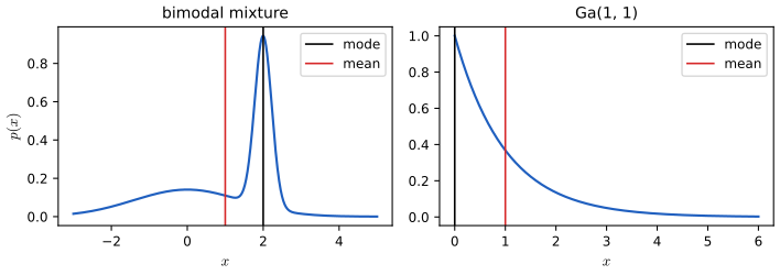
pp. 349–350 The simplest approximation is to maximise the posterior and pretend all the mass sits at the maximiser, \[ \hat\theta=\argmax_\theta\ \big[\log p(\theta)+\log p(\mathcal D\given\theta)\big],\qquad p(\theta\given\mathcal D)\approx\delta(\theta-\hat\theta). \tag{7.18, 7.19} \] It can use any optimiser of Chapter 6, but it has three problems. No uncertainty. A point carries no error bar, and a plug-in predictive can be confidently wrong (Section 3.2.2 of the book). The mode is often atypical. For a bimodal density with one narrow tall peak the mode sits far from most of the mass; for a skewed density such as Ga\((1,1)\) the mode is 0 while the mean is 1 (Figure 7.2), which is why a variance parameter in a hierarchical model should not be summarised by its MAP value. No reparameterisation invariance. The mode of a density moves under a nonlinear change of variables, because the density picks up a Jacobian (gap 7.3); the likelihood, being a function rather than a density in \(\theta\), does not have this problem, and neither do posterior expectations, since the change of measure is part of the integral.
Filling the gap 7.3: the mode of a transformed density is not the transformed mode pp. 349–350, Figure 7.2, Section 2.5.1
Derivation
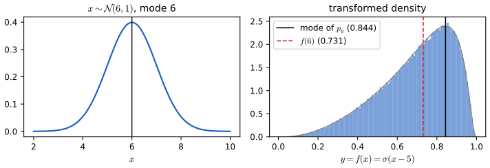
Let \(x\) have density \(p_x\) and let \(y=f(x)\) with \(f\) differentiable and strictly increasing. The change-of-variables formula is \(p_y(y)=p_x(f^{-1}(y))\,\big|\frac{\d f^{-1}}{\d y}\big|\); the Jacobian factor is what moves the mode. If \(\hat y=\argmax p_y\) and \(\hat x=\argmax p_x\), then \(p_y'(\hat y)=0\) reads \[ p_x'(x)\Big(\frac{\d x}{\d y}\Big)^2+p_x(x)\frac{\d^2x}{\d y^2}=0\quad\text{at }x=f^{-1}(\hat y), \] whereas \(f(\hat x)\) would require \(p_x'(\hat x)=0\); the two agree only when \(\d^2x/\d y^2=0\), i.e. \(f\) is affine. Worked example from the book. Let \(x\sim\mathcal N(6,1)\) and \(y=\sigma(x-5)\), so \(x=5+\operatorname{logit}y\), \(\d x/\d y=1/(y(1-y))\) and \[ p_y(y)=\frac{\mathcal N(5+\operatorname{logit}y\given6,1)}{y(1-y)}\ \Rightarrow\ \log p_y=-\tfrac12(u-1)^2-\log y-\log(1-y)+\const,\quad u=\operatorname{logit}y. \] Differentiating in \(y\) (with \(\d u/\d y=1/(y(1-y))\)) and multiplying by \(y(1-y)\): \(-(u-1)-(1-y)+y=0\), i.e. \(\operatorname{logit}(y)=2y\). The root is \(\hat y\approx0.8439\), whereas \(f(\hat x)=\sigma(6-5)=0.7311\) (see the own figure after this box; confirmed numerically). Why the likelihood is immune: \(L(\theta)=p(\mathcal D\given\theta)\) is a function of the parameter value, and \(L(\theta)=\tilde L(\phi)\) when \(\phi=g(\theta)\) is a relabelling, so \(\argmax\tilde L=g(\argmax L)\); no density, hence no Jacobian. Why posterior expectations are immune: \(\int g(\theta)p(\theta\given\mathcal D)\,\d\theta\) is a number that does not depend on the coordinates because \(p(\theta\given\mathcal D)\,\d\theta\) is a measure.
7.4.2 Grid approximation
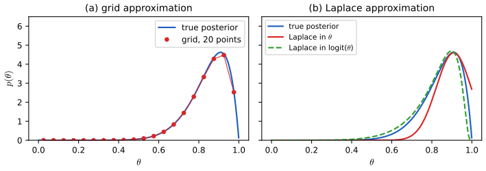
pp. 350–351 Partition the parameter space into \(K\) cells of volume \(\Delta\) centred at \(\theta_k\) and set \[ \tilde p_k=p(\mathcal D\given\theta_k)p(\theta_k),\quad p_k=\frac{\tilde p_k}{\sum_{k'}\tilde p_{k'}},\quad p(\theta\in r_k\given\mathcal D)\approx p_k\Delta,\quad p(\mathcal D)\approx\sum_k\Delta\tilde p_k \tag{7.20–7.22} \] (the book's \(p_k\Delta\) is the cell probability; the density estimate in the cell is \(p_k/\Delta\) when \(\sum_kp_k=1\), as the code uses). In one dimension this captures the skew of the Beta(11,2) posterior well (Figure 7.3a); the trouble is the cost, \(K^D\) points in \(D\) dimensions (gap 7.4). The evidence estimate is also useful: with \(K=20{,}000\) cells it equals \(\log B(11,2)=-4.8828\) to six digits, and even \(K=20\) gives \(-4.8694\).
Filling the gap 7.4: the grid estimate as a Riemann sum, its error, and the curse of dimensionality p. 351, (7.20)–(7.22)
Derivation
Let \(h(\theta)=p(\mathcal D\given\theta)p(\theta)\) be continuous on a bounded region of volume \(V\). Partition it into \(K\) congruent cells of volume \(\Delta=V/K\) with centres \(\theta_k\). The sum \(\Delta\sum_kh(\theta_k)\) is the midpoint Riemann sum of \(\int h\). On a cell of side \(s\) (so \(\Delta=s^D\)), Taylor expansion about the centre, \(h(\theta)=h(\theta_k)+\nabla h^\T(\theta-\theta_k)+\frac12(\theta-\theta_k)^\T\nabla^2h(\theta-\theta_k)+\cdots\), shows that the integral of the linear term over the symmetric cell vanishes, so the cell error is \(\frac1{24}s^2\Delta\operatorname{tr}\nabla^2h\) plus higher order terms; summing over \(K\) cells the total error is \(O(s^2)=O(K^{-2/D})\) for fixed region. To reach a given accuracy \(\varepsilon\) one needs \(s\propto\varepsilon^{1/2}\) and so \(K\propto\varepsilon^{-D/2}\) cells: exponential in \(D\). With 20 points per axis, \(D=10\) needs \(20^{10}\approx10^{13}\) evaluations. The normalised weights \(p_k\) inherit the same error because \(p(\mathcal D)\) is the common denominator.
7.4.3 Laplace (quadratic) approximation
pp. 351–352 Write the posterior as \(p(\theta\given\mathcal D)=\frac1Ze^{-E(\theta)}\) with energy \(E(\theta)=-\log p(\theta,\mathcal D)\) and \(Z=p(\mathcal D)\). A second-order Taylor expansion about the mode \(\hat\theta\) (where the gradient vanishes) gives \[ \hat p(\theta\given\mathcal D)=\mathcal N(\theta\given\hat\theta,\bm H^{-1}),\qquad Z\approx e^{-E(\hat\theta)}(2\pi)^{D/2}|\bm H|^{-1/2}, \tag{7.27, 7.28} \] with \(\bm H\) the Hessian of \(E\) at the mode. It needs only an optimiser and one Hessian (or a diagonal or low-rank approximation in high dimensions); applications are in Chapter 15 (Bayesian logistic regression), Chapter 17 (Bayesian neural networks) and Chapter 4 (Gaussian Markov random fields).
Filling the gap 7.5: derivation of the Laplace approximation, its failure in \(\theta\) and the logit fix pp. 351–352, (7.24)–(7.28)
Derivation
Derivation. Assume \(E\) is twice differentiable with a strict local minimum at \(\hat\theta\), so \(\nabla E(\hat\theta)=\bm 0\) and \(\bm H=\nabla^2E(\hat\theta)\) is positive definite. Taylor's theorem gives \(E(\theta)\approx E(\hat\theta)+\frac12(\theta-\hat\theta)^\T\bm H(\theta-\hat\theta)\) (7.25 with \(\bm g=\bm0\)). Substituting, \(\hat p(\theta,\mathcal D)=e^{-E(\hat\theta)}\exp(-\frac12(\theta-\hat\theta)^\T\bm H(\theta-\hat\theta))\) (7.26). The Gaussian integral \(\int\exp(-\frac12 u^\T\bm Hu)\,\d u=(2\pi)^{D/2}|\bm H|^{-1/2}\) gives the normaliser \(\hat Z\) in (7.28), and dividing \(\hat p(\theta,\mathcal D)\) by it gives \(\mathcal N(\hat\theta,\bm H^{-1})\) (7.27). The approximation is exact in the limit of large data (Bernstein–von Mises) but only local: it matches the value and curvature at one point.
The running example in \(\theta\). \(E(\theta)=-N_1\log\theta-N_0\log(1-\theta)\) (up to a constant; with a uniform prior), minimised at \(\hat\theta=N_1/(N_1+N_0)=10/11\) with \(E''(\hat\theta)=N_1/\hat\theta^2+N_0/(1-\hat\theta)^2=133.1\), so the variance is \(1/133.1=0.00751\) and the standard deviation \(0.0867\). The Gaussian puts mass \(1-\Phi\big((1-\tfrac{10}{11})/0.0867\big)=1-\Phi(1.049)\approx0.147\) above 1, which is impossible for a probability: the support constraint is ignored. The log-evidence estimate is \(-4.8776\) against the exact \(-4.8828\) (a 0.005 error), but the density is poor (Figure 7.3b).
Fix: change variables. Work with \(\alpha=\operatorname{logit}\theta\in\mathbb R\) and \(\theta=\sigma(\alpha)\). The posterior density of \(\alpha\) is \(p(\theta\given\mathcal D)\,\sigma'(\alpha)\), with \(\sigma'=\sigma(1-\sigma)\), so with \(a=N_1+1\), \(b=N_0+1\) the log joint (including the Jacobian) is \(a\log\sigma(\alpha)+b\log(1-\sigma(\alpha))\). Its derivative is \(a(1-\sigma)-b\sigma\), zero at \(\hat\sigma=a/(a+b)\), i.e. \(\hat\alpha=\log(a/b)=\log(11/2)=1.705\), and the curvature is \((a+b)\hat\sigma(1-\hat\sigma)=13\cdot\frac{11}{13}\cdot\frac{2}{13}=\frac{22}{13}=1.692\), giving variance \(13/22=0.591\). The Laplace density in \(\theta\) is then \(\mathcal N(\operatorname{logit}\theta\given\hat\alpha,0.591)/(\theta(1-\theta))\), which lives on \((0,1)\) and is skewed like the truth. The L1 distance to the exact posterior drops from 0.255 to 0.161; the evidence estimate is \(-4.9262\) (error \(-0.043\)), slightly worse than in \(\theta\), so a better density does not automatically mean a better evidence estimate. Both statements were confirmed numerically.
7.4.4 Variational inference
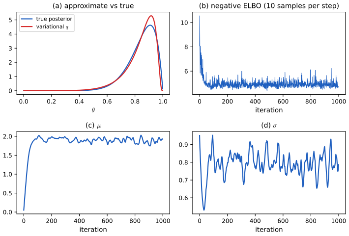
pp. 352–353 Variational inference (VI, also variational Bayes) also uses optimisation, but searches a family \(\mathcal Q\) of tractable distributions \(q(\theta\given\psi)\) for the one closest in KL to the posterior: \[ \psi^*=\argmin_\psi\KL\big(q(\theta\given\psi)\,\|\,p(\theta\given\mathcal D)\big)=\argmax_\psi\ \ELBO(\psi),\quad \ELBO(\psi)=\E_{q(\theta\given\psi)}[\log p(\mathcal D\given\theta)+\log p(\theta)-\log q(\theta\given\psi)] \tag{7.29–7.34} \] (gap 7.6). Because \(\KL\ge0\), \(\ELBO(\psi)\le\log p(\mathcal D)\): the evidence lower bound. A Gaussian \(q=\mathcal N(\mu,\Sigma)\) differs from the Laplace approximation in that its parameters are optimised, not tied to the mode and Hessian; a diagonal \(\Sigma\) gives the mean-field approximation. Automatic differentiation variational inference (ADVI, Kucukelbir et al. 2017) makes the method turn-key: map constrained parameters to \(\mathbb R^D\), take a Gaussian there, and estimate the ELBO gradient by the reparameterisation trick with automatic differentiation. Details, including SVI, amortised inference, mixtures of variational families and alternative divergences, are in Chapter 10; the identical bound is the training objective of the VAE of Chapter 21.
Filling the gap 7.6: the ELBO identity, and the reparameterised gradient for the example pp. 352–353, (7.29)–(7.34)
Derivation
Identity. For any \(q\) with support containing that of the posterior, \[ \KL(q\,\|\,p(\cdot\given\mathcal D))=\E_q\Big[\log\frac{q(\theta)}{p(\theta,\mathcal D)/p(\mathcal D)}\Big]=\E_q[\log q(\theta)-\log p(\theta,\mathcal D)]+\log p(\mathcal D)=-\ELBO+\log p(\mathcal D), \] using \(p(\theta\given\mathcal D)=p(\theta,\mathcal D)/p(\mathcal D)\) and that \(\log p(\mathcal D)\) does not depend on \(\theta\) so comes out of the expectation. Thus \(\log p(\mathcal D)=\ELBO(\psi)+\KL(q\|p)\) (7.33). The term \(\log p(\mathcal D)\) is constant in \(\psi\), so minimising the KL is the same as maximising \(\ELBO\), which needs only the unnormalised joint. Nonnegativity of KL: by Jensen applied to the concave \(\log\), \(-\KL(q\|p)=\E_q[\log(p/q)]\le\log\E_q[p/q]=\log\int p=0\); the bound is tight iff \(q=p\) almost everywhere. For the running example the optimum Gaussian-in-logit has \(\mu^*=1.911\), \(\sigma^*=0.801\), ELBO \(-4.9051\) and gap \(\KL(q\|p)=0.0223\) (the divergence is the same in the \(\theta\) and \(\alpha\) coordinates), so the bound is within \(0.03\) of \(\log p(\mathcal D)=-4.8828\) (the sum of the gap and the ELBO equals the log-evidence to five digits; confirmed numerically).
Reparameterised gradient. Write \(z=\mu+\sigma\varepsilon\) with \(\varepsilon\sim\mathcal N(0,1)\), so \(\ELBO(\mu,\sigma)=\E_\varepsilon[\ell(\mu+\sigma\varepsilon)]+\log\sigma+\frac12\log(2\pi e)\) where \(\ell(z)=a\log\sigma(z)+b\log(1-\sigma(z))\) is the log joint in \(z\) with its Jacobian, and \(\log\sigma+\tfrac12\log(2\pi e)\) is the entropy of \(q\). Differentiating under the expectation (dominated convergence: \(\ell'\) is bounded by \(\max(a,b)\)), with \(g(z)=\ell'(z)=a(1-\sigma(z))-b\sigma(z)\), \[ \frac{\partial\ELBO}{\partial\mu}=\E_\varepsilon[g(\mu+\sigma\varepsilon)],\qquad\frac{\partial\ELBO}{\partial\log\sigma}=\E_\varepsilon[g(\mu+\sigma\varepsilon)\,\varepsilon\sigma]+1. \] Replacing the expectation by an average over a few draws gives an unbiased stochastic gradient, which is what the code feeds to Adam; no derivative of \(q\) with respect to its parameters through the sampling is needed because all the randomness sits in \(\varepsilon\).
7.4.5 Markov chain Monte Carlo (MCMC)
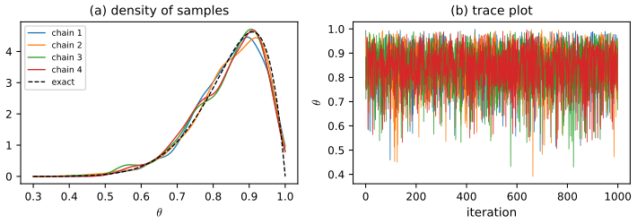
pp. 354–355 VI is fast but biased by the choice of \(\mathcal Q\). A nonparametric alternative represents the posterior by samples, \(q(\theta)\approx\frac1S\sum_s\delta(\theta-\theta_s)\), obtained without ever computing \(p(\mathcal D)\). In low dimension, importance sampling works (Chapter 11); in high dimension one uses MCMC (Chapter 12). The Metropolis–Hastings algorithm proposes \(\theta'\sim q(\theta'\given\theta)\) and moves there with a probability that depends on the unnormalised ratio \(p(\mathcal D,\theta')/p(\mathcal D,\theta)\) (7.35), in which the evidence cancels (gap 7.7); the random-walk version uses a Gaussian proposal. Gibbs sampling samples each variable from its full conditional, and Hamiltonian Monte Carlo (HMC) uses the gradient of the log joint to make long informed moves. Figure 7.5 applies HMC to the example on the logit scale.
Filling the gap 7.7: why the Metropolis–Hastings rule leaves the posterior invariant pp. 354–355, (7.35)
Derivation
Let \(\pi(\theta)\propto h(\theta)=p(\theta,\mathcal D)\) be the target and \(q(\theta'\given\theta)\) a proposal. The Metropolis–Hastings kernel proposes \(\theta'\sim q(\cdot\given\theta)\) and accepts it with probability \(\alpha(\theta,\theta')=\min\{1,r\}\), \(r=\dfrac{h(\theta')q(\theta\given\theta')}{h(\theta)q(\theta'\given\theta)}\); otherwise the chain stays. The ratio involves \(h\) only through \(h(\theta')/h(\theta)\), so the constant \(1/p(\mathcal D)\) cancels: this is why (7.35) can be evaluated without the evidence. For a symmetric proposal (random walk) \(r=h(\theta')/h(\theta)\).
Detailed balance. For \(\theta\ne\theta'\) the transition density is \(K(\theta'\given\theta)=q(\theta'\given\theta)\alpha(\theta,\theta')\). Then \[ \pi(\theta)K(\theta'\given\theta)\propto h(\theta)q(\theta'\given\theta)\min\Big\{1,\frac{h(\theta')q(\theta\given\theta')}{h(\theta)q(\theta'\given\theta)}\Big\}=\min\{h(\theta)q(\theta'\given\theta),\,h(\theta')q(\theta\given\theta')\}, \] which is symmetric in \((\theta,\theta')\), so \(\pi(\theta)K(\theta'\given\theta)=\pi(\theta')K(\theta\given\theta')\). Integrating this identity over \(\theta\) and using \(\int K(\theta\given\theta')\,\d\theta=1-\)(rejection mass at \(\theta'\)) (the point mass at \(\theta'\) handles \(\theta=\theta'\)) shows \(\int\pi(\theta)K(\theta'\given\theta)\,\d\theta=\pi(\theta')\): \(\pi\) is stationary. If the chain is also irreducible and aperiodic (e.g. a Gaussian random walk on a continuous support), the distribution of \(\theta_t\) converges to \(\pi\) and ergodic averages \(\frac1S\sum_sg(\theta_s)\) converge to \(\E_\pi[g]\) (the Markov chain law of large numbers; see Chapter 12). The samples are correlated, so the effective sample size is smaller than \(S\); a step that is too small accepts nearly everything yet crawls, one that is too large is rarely accepted (the demonstration lets you see both). On a finite three-state example the kernel was confirmed numerically to satisfy detailed balance and \(\pi P=\pi\).
7.4.6 Sequential Monte Carlo
p. 355 MCMC is a local search that moves through the state space. Sequential Monte Carlo (SMC) instead propagates a population of samples through a sequence of distributions that run from simple to the target, which is more like tree search and avoids getting stuck in one mode. Its classic use is sequential (online) Bayesian inference, recursively computing \(p(\theta_t\given\mathcal D_{1:t})\) as data arrive, and applied to dynamical models it is particle filtering. Details are in Chapter 13 and, for state-space models, Chapter 29.
7.4.7 Challenging posteriors
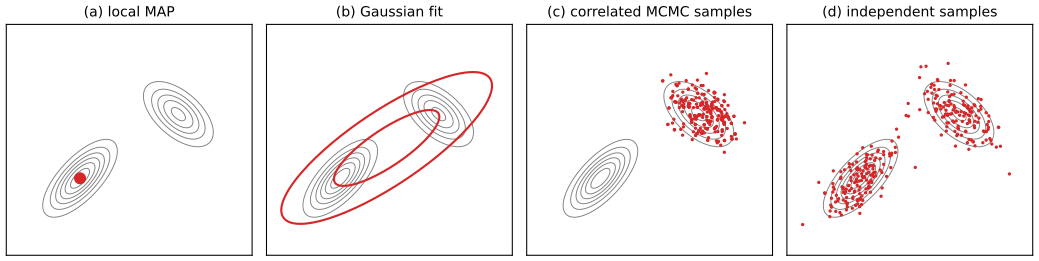
p. 356 High-dimensional, multimodal posteriors are hard. Figure 7.6 in the book (a sketch) contrasts four summaries of a bimodal 2-d posterior: a local MAP point, a Gaussian fit (Laplace or VI), correlated MCMC samples stuck near one mode, and ideal independent samples from the whole support. My own figure makes the same comparison with a computed two-component mixture.
7.5 Evaluating approximate inference algorithms
pp. 356–357 Approximations differ in speed, accuracy, generality and simplicity, so a fair comparison is subtle. If a trusted reference posterior exists, one can plot the accuracy-versus-time trade-off, e.g. \(\KL(p(\theta\given\mathcal D)\,\|\,q_t(\theta))\) after \(t\) units of compute, or use another distance such as a Wasserstein distance. The demonstration computes this KL for the one-dimensional example. Usually the true posterior is not available, so one evaluates the quality of the predictive distribution out of sample, as in cross-validation, or its Bayes risk under a loss \(\ell\), \[ R=\E_{p^*(x,y)}\big[\ell\big(y,q(y\given x,\mathcal D)\big)\big],\qquad q(y\given x,\mathcal D)=\int p(y\given x,\theta)\,q(\theta\given\mathcal D)\,\d\theta, \tag{7.36} \] (Kass and coauthors' proposal), or in a downstream task such as active or continual learning. Specialised diagnostics exist for VI and for Monte Carlo methods (see the book's references). The predictive-evaluation ideas, calibration and proper scoring rules, are developed in Chapter 14, and decision-theoretic loss in Chapter 34.
See also: Bayesian and Probabilistic ML, 10.1 variational inference; 11.2 MCMC; 4.4 the Laplace approximation.
Practice problems
The book has no exercises for this chapter. These three short problems are my own.
Practice problem 7.1 (Laplace evidence for a Gaussian). Let \(p(\theta,\mathcal D)=c\,\exp(-\frac12(\theta-m)^2/s^2)\) in one dimension. Show that the Laplace estimate (7.28) of the evidence is exact.
Solution
Here \(E(\theta)=-\log c+\frac12(\theta-m)^2/s^2\), minimised at \(\hat\theta=m\) with \(E(\hat\theta)=-\log c\) and \(H=1/s^2\). Then \(\hat Z=e^{-E(\hat\theta)}(2\pi)^{1/2}H^{-1/2}=c\sqrt{2\pi}\,s\), which equals \(\int c\,e^{-(\theta-m)^2/(2s^2)}\,\d\theta=c\sqrt{2\pi}s\) exactly. A quadratic energy has no cubic or higher terms to neglect, so the approximation is exact; for the beta example it is not, and the errors above are the price of non-Gaussianity.
Practice problem 7.2 (grid size). With the uniform prior and 10 heads and 1 tail, how many equally spaced cells are needed for the grid estimate of \(\log p(\mathcal D)\) to be within \(10^{-3}\) of \(\log B(11,2)\)? Use the code.
Solution
The midpoint rule has error \(O(K^{-2})\) (gap 7.4). Evaluating \(\log\big(\Delta\sum_k\tilde p_k\big)\) for \(K=20,50,100,200\) gives errors \(0.0134,\ 0.0022,\ 5.5\times10^{-4},\ 1.4\times10^{-4}\) (a doubling of \(K\) divides the error by about four), so about \(K=75\) cells reach \(10^{-3}\) and \(K=100\) is comfortably inside. In ten dimensions the same per-axis resolution would need \(75^{10}\approx6\times10^{18}\) evaluations.
Practice problem 7.3 (a skewed posterior). A variance \(\sigma^2\) has posterior \(\operatorname{Ga}(1,1)\) (shape 1, rate 1). Give the MAP, mean and median, and the MAP of \(\log\sigma^2\). Which would you report?
Solution
The density is \(e^{-x}\), \(x>0\): mode 0, mean 1, median \(\log2=0.693\). For \(u=\log x\) the density is \(p_u(u)=e^{u}e^{-e^{u}}\) (Jacobian \(\d x/\d u=e^u\)), maximised where \(1-e^u=0\), i.e. \(u=0\), so the MAP of \(\log\sigma^2\) is 0 and corresponds to \(\sigma^2=1\), not 0: the MAP changed with the parameterisation, as in gap 7.3. The mean (or median) is the sensible summary: the mode \(0\) is a degenerate, unrepresentative variance.
Demonstration
| Page | What it shows | In the notes |
|---|---|---|
| Approximating a posterior | The beta-Bernoulli posterior against the MAP point, a grid, the Laplace approximation in \(\theta\) and in the logit, a Gaussian variational fit and random-walk MCMC, with KL to the truth and the evidence estimate. Presets: 1 the book's example; 2 a coarse grid; 3 all heads (no interior mode); 4 lots of data; 5 a tiny MCMC step; 6 a good step. | Section 7.4 |
The Python code that produces every figure of this page is code/ch07_inference_overview.py (see the code index). Companion demos: conjugate priors.
Notes on the book
Points where the book is imprecise
- (7.20) and (7.22), grid normalisation. If \(p_k=\tilde p_k/\sum\tilde p_{k'}\) sums to one, then \(p_k\) is already the cell probability, and \(p(\theta\in r_k\given\mathcal D)\approx p_k\), not \(p_k\Delta\); the density estimate in the cell is \(p_k/\Delta\). The factor \(\Delta\) belongs in the evidence (7.22), \(p(\mathcal D)\approx\Delta\sum_k\tilde p_k\). The notes and code use the consistent version.
References
- Murphy, K. P. (2023). Probabilistic Machine Learning: Advanced Topics. MIT Press, Cambridge, MA. Chapter 7, pp. 345–357. probml.github.io/pml-book/book2.html.
- Kucukelbir, A., Tran, D., Ranganath, R., Gelman, A. and Blei, D. M. (2017). Automatic differentiation variational inference. Journal of Machine Learning Research, 18(14), 1–45.
- Hastings, W. K. (1970). Monte Carlo sampling methods using Markov chains and their applications. Biometrika, 57(1), 97–109.
- Metropolis, N., Rosenbluth, A. W., Rosenbluth, M. N., Teller, A. H. and Teller, E. (1953). Equation of state calculations by fast computing machines. Journal of Chemical Physics, 21(6), 1087–1092.
- Kingma, D. P. and Ba, J. (2015). Adam: a method for stochastic optimization. International Conference on Learning Representations.
- Tierney, L. and Kadane, J. B. (1986). Accurate approximations for posterior moments and marginal densities. Journal of the American Statistical Association, 81(393), 82–86.
The numerical statements in the text (the grid and Laplace evidence estimates, the Hessians, the non-invariance of the mode, the ELBO identity and the variational optimum, the HMC mean and acceptance rate, detailed balance of the Metropolis–Hastings kernel, conjugacy by adding natural parameters, the prior-expectation form of the evidence, and the interactive demonstration) were confirmed numerically.