Gradient Descent
A network is trained by minimising an error function \(E(\bw)\) over its weights and biases. There is no closed-form minimiser, so we move through weight space in small steps guided by the gradient. This chapter studies the shape of the error surface near a minimum (Section 7.1), the family of gradient methods used in deep learning: batch, stochastic and mini-batch gradient descent and how to start them (7.2), why plain gradient descent is slow when the curvature differs between directions, and how momentum, learning-rate schedules and per-weight step sizes (AdaGrad, RMSProp, Adam) help (7.3), and finally how normalising inputs and hidden variables makes the error surface easier to descend (7.4).
Ch. 1 Deep learning revolution Ch. 2 Probabilities Ch. 3 Standard distributions Ch. 4 Regression Ch. 5 Classification Ch. 6 Deep neural networks Ch. 7 Gradient descent Ch. 8 Backpropagation Ch. 9 Regularization Ch. 10 Convolutional networks Ch. 11 Structured distributions Ch. 12 Transformers Ch. 13 Graph neural networks Ch. 14 Sampling Ch. 15 Discrete latent variables Ch. 16 Continuous latent variables Ch. 17 GANs Ch. 18 Normalizing flows Ch. 19 Autoencoders Ch. 20 Diffusion models Appendices A to C
How to read these notes
They follow the book. Sections carry the book's numbers (7.1, 7.3.2, ...) and every displayed equation that appears in the book carries the book's own equation number, e.g. (7.16), so the notes can be read next to the book. Equations without a number are steps that the book skips.
Filling the gaps. Wherever the book states a result without proof, says it "can be shown", or leaves it to an exercise, an orange Filling the gap box or a proof gives the full argument. Proofs and derivations start hidden: open one with its bar, or use the button below.
Figures and demonstrations. All eight figures of the chapter are schematic in the book; here each one is computed from an explicit function, data set or simulation by the Python code. Six supplementary figures (7.S1 to 7.S6, our own) illustrate the gaps that are filled. The ▶ Demo boxes open an interactive demonstration already set to the case being discussed.
Main reference
C. M. Bishop and H. Bishop, Deep Learning: Foundations and Concepts, Springer (2024), Chapter 7, pages 209–232. Section, equation, figure and exercise numbers below refer to this book. Further reading is listed in the references; the book's website is www.bishopbook.com.
The explanations, derivations, figures and code are my own; equations are cited by their numbers in the book.
Companion course: Bayesian and Probabilistic Machine Learning
Part of this chapter overlaps the companion course Bayesian and Probabilistic Machine Learning (Bishop 2006). Where the full proof is already there, these notes give the statement and a short argument and link it.
- Error surfaces and weight-space symmetries: Section 5.1.1 and Section 5.2.1 (here 7.1).
- The local quadratic approximation, the Hessian's eigenvectors and the elliptical contours: Section 5.2.2, Result 5.5 (here 7.1.1, Exercises 7.1–7.3, 7.6).
- Why gradients pay: the \(W(W+3)/2\) count and the \(O(W^3)\) versus \(O(W^2)\) argument: Section 5.2.3 (here 7.2.1, Exercise 7.7).
- Batch and on-line gradient descent: Section 5.2.4 and sequential least squares in Section 3.1.3 (here 7.2.2–7.2.3).
- Gradient descent on a quadratic as a filter on the Hessian's eigen-directions (early stopping): Result 5.13 in Section 5.5.2 (here 7.3).
- Sequential estimation and the Robbins–Monro conditions on the step sizes: Section 2.3.5, Result 2.15 (here 7.3.2).
- Moments of the sample mean: Result 1.7 (here Exercise 7.8); the Hessians of least squares and of logistic regression: Section 3.1.1 and Section 4.3.3 (here Exercises 7.4 and 7.5).
- Demonstration: the backpropagation demo, where a network is trained by Adam with an adjustable step size.
The chapter at a glance
- 7.1 The error is a surface over weight space. Near a stationary point it is a quadratic described by the Hessian; positive definiteness is sufficient for a strict local minimum, and positive semi-definiteness is necessary (Result 7.2). Weight-space symmetries make minima come in families, and for ReLU networks in continuous ones (Filling the gap 7.2).
- 7.2 Gradient descent and its stochastic and mini-batch versions. A small enough step always decreases a smooth error (Result 7.3); the mini-batch gradient is unbiased with variance \(\propto 1/B\) (Result 7.4); He initialisation keeps the second moment of the pre-activations constant through a deep ReLU network (Result 7.5, with a correction to (7.22)).
- 7.3 On a quadratic, gradient descent contracts each eigen-direction by \(1-\eta\lambda_i\): stable iff \(\eta<2/\lambda_{\max}\), best rate \((\kappa-1)/(\kappa+1)\) (Result 7.6). Momentum improves this to \((\sqrt\kappa-1)/(\sqrt\kappa+1)\) (Result 7.7), Nesterov momentum to \(1-1/\sqrt\kappa\) (Result 7.8). Constant-rate SGD stalls at a noise floor that a decaying schedule removes (Result 7.9). Adam's bias correction, sign-like first step, scale invariance and step bound (Result 7.10).
- 7.4 Standardising the inputs improves the conditioning of the Hessian (Filling the gap 7.7). Batch and layer normalisation have explicit gradients that are projections (Result 7.11), make the layer invariant to the scale of its weights, and so tune their own effective learning rate (Filling the gap 7.9).
Notation. \(\bw\in\R^W\) collects all weights and biases; \(E(\bw)=\sum_{n=1}^NE_n(\bw)\) is the training error; \(\nabla E\) its gradient and \(\bH=\nabla\nabla E\) its Hessian, with eigenpairs \((\lambda_i,\bu_i)\); \(\eta\) is the learning rate and \(\tau\) the step index; \(\kappa=\lambda_{\max}/\lambda_{\min}\) is the condition number. In layer \(l\), \(a^{(l)}_i\) is a pre-activation and \(z^{(l)}_i=h(a^{(l)}_i)\) an activation. A mini-batch has \(B\) (in Section 7.4.2: \(K\)) examples.
Printings. The first printing of the book has a few slips in this chapter (a missing minus sign in (7.64), a sign error in Algorithm 7.4, wrong indices in (7.22) and (7.59), an imprecise "necessary and sufficient" condition). Each is flagged with an Erratum note where it occurs, and the list with the evidence is in the summary at the end of Section 7.4.
pp. 209–210 The parameters of a network are chosen by minimising an error function, usually a negative log likelihood (Section 6.4 of the book). Evaluating \(E\) alone at many trial points would be hopelessly slow; instead we use its derivatives, which backpropagation (Chapter 8) delivers at a cost comparable to one evaluation of \(E\). The book stresses a difference from classical statistics: with far more parameters than data points, the goal is not the exact minimiser of the training error but a solution that generalises, and the optimisation algorithm itself (its noise, its step sizes, its starting point) shapes which solution is found.
7.1 Error surfaces
See also the companion course, Section 5.2.1 (parameter optimization) and Section 5.1.1 (weight-space symmetries).
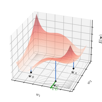
pp. 210–211 Group all weights and biases into one vector \(\bw\) and think of \(E(\bw)\) as a surface over weight space (Figure 7.1). A small step \(\delta\bw\) changes the error by
\[ \delta E\simeq\delta\bw^\T\nabla E(\bw), \tag{7.1} \]so \(\nabla E\) points in the direction in which \(E\) increases fastest, and at a minimum of a smooth error
\[ \nabla E(\bw)=\bzero, \tag{7.2} \]since otherwise a small step along \(-\nabla E\) would lower the error. Points where the gradient vanishes are stationary points: minima, maxima or saddle points. A minimum with the smallest value of \(E\) over all of weight space is a global minimum; others are local minima.
Filling the gap 7.1: why \(-\nabla E\) is the steepest descent direction, and why the gradient vanishes at a minimum p. 210, (7.1)–(7.2)
The book uses both facts without proof. Assume \(E\) is differentiable at \(\bw\).
Derivation
(7.1). Differentiability means \[E(\bw+\delta\bw)=E(\bw)+\delta\bw^\T\nabla E(\bw)+o(\|\delta\bw\|),\] so the first-order change is \(\delta\bw^\T\nabla E\).
Steepest direction. Among unit vectors \(\bd\), the directional derivative \(\bd^\T\nabla E\) satisfies \(|\bd^\T\nabla E|\le\|\bd\|\,\|\nabla E\|=\|\nabla E\|\) by the Cauchy–Schwarz inequality, with equality iff \(\bd=\pm\nabla E/\|\nabla E\|\). So the increase is fastest along \(+\nabla E\) and the decrease fastest along \(-\nabla E\), at rate \(\|\nabla E\|\). Note that "steepest" depends on the Euclidean norm used to measure step length: in another norm \(\|\bd\|_{\bm M}^2=\bd^\T\bm M\bd\) the steepest direction is \(-\bm M^{-1}\nabla E\), which is the idea behind preconditioning and, loosely, behind the per-weight scalings of Section 7.3.3.
(7.2). Suppose \(\bw^\star\) is a local minimum and \(\bg=\nabla E(\bw^\star)\ne\bzero\). For small \(\epsilon>0\), \[E(\bw^\star-\epsilon\bg)=E(\bw^\star)-\epsilon\|\bg\|^2+o(\epsilon),\] which is below \(E(\bw^\star)\) once \(\epsilon\) is small enough that the \(o(\epsilon)\) term is smaller than \(\epsilon\|\bg\|^2\). This contradicts minimality, so \(\bg=\bzero\). The condition is necessary, not sufficient: maxima and saddle points satisfy it too. ∎
Equivalent minima. The book recalls (Section 6.2.4) that in a two-layer network with \(M\) hidden units each point of weight space has \(M!\,2^M\) equivalent points that compute the same function, so every minimum comes with many copies. For ReLU units the count is different, and the copies are no longer isolated:
Filling the gap 7.2: weight-space symmetries of ReLU networks give flat valleys and a singular Hessian p. 211
The \(M!\,2^M\) count (permutations of hidden units, and sign flips \(\bw\to-\bw\) that use \(\tanh(-a)=-\tanh(a)\)) is for odd activation functions. The rectified linear unit is not odd, but it is positively homogeneous, and that produces a continuous family of equivalent weights.
Derivation
Rescaling symmetry. For \(c>0\), \[\ReLU(ca)=\max(0,ca)=c\ReLU(a).\] Take a hidden unit \(j\) with incoming weights and bias \(\bw_j\) and outgoing weights \(\bv_j\). Replacing \((\bw_j,\bv_j)\) by \((c\bw_j,\bv_j/c)\) multiplies its activation by \(c\) and its outgoing contributions by \(1/c\), so the network function, and hence \(E\), is unchanged. Each hidden unit therefore contributes a one-parameter curve \(c\mapsto\bw(c)\) of weight vectors with the same error. (Permutations of hidden units remain symmetries; sign flips do not.)
Consequence for the Hessian. Let \(\bw^\star\) be a local minimum and \(\bw(c)\) a smooth curve with \(\bw(1)=\bw^\star\) along which \(E\) is constant. Differentiate \(E(\bw(c))=E(\bw^\star)\) twice at \(c=1\), with \(\bm t=\bw'(1)\): \[ \bm t^\T\nabla E(\bws)=0,\qquad \bm t^\T\bH\bm t+\bw''(1)^\T\nabla E(\bws)=0. \] Since \(\nabla E(\bws)=\bzero\), \(\bm t^\T\bH\bm t=0\). At a minimum \(\bH\) is positive semi-definite (Result 7.2), and for a positive semi-definite matrix \(\bm t^\T\bH\bm t=0\) implies \(\bH\bm t=\bzero\) (write \(\bH=\bm R^\T\bm R\); then \(\|\bm R\bm t\|^2=0\), so \(\bm R\bm t=\bzero\)). Hence \(\bH\) has a zero eigenvalue for every hidden unit, with eigenvector \(\bm t=(\bw_j,-\bv_j)\) restricted to that unit's weights. Minima of ReLU networks are therefore never strict and the condition number \(\lambda_{\max}/\lambda_{\min}\) of the Hessian is infinite. The convergence analysis of Section 7.3 then applies on the subspace orthogonal to these flat directions, along which gradient descent simply does not move to first order. ∎
It was once feared that gradient methods would be trapped in poor local minima. The book notes that in practice large networks reach solutions of similar quality from many different starting points (more on this in Section 9.3.2 of the book).
7.1.1 Local quadratic approximation
See also the companion course, Section 5.2.2 and Result 5.5, which prove the same eigen-expansion for Bishop (2006).
pp. 211–213 A second-order Taylor expansion about a point \(\widehat\bw\) gives
\[ E(\bw)\simeq E(\widehat\bw)+(\bw-\widehat\bw)^\T\bb+\tfrac12(\bw-\widehat\bw)^\T\bH(\bw-\widehat\bw), \tag{7.3} \]where
\[ \bb\equiv\nabla E\big|_{\bw=\widehat\bw}, \tag{7.4} \] \[ \bH(\widehat\bw)=\nabla\nabla E(\bw)\big|_{\bw=\widehat\bw}, \tag{7.5} \]so that the gradient is approximated by
\[ \nabla E(\bw)=\bb+\bH(\bw-\widehat\bw). \tag{7.6} \]Definition 7.1 (Hessian; positive definite) pp. 211–212, (7.5), (7.12)
The Hessian \(\bH\) is the \(W\times W\) matrix with entries \(H_{ij}=\partial^2E/\partial w_i\partial w_j\). When \(E\) has continuous second derivatives the order of differentiation does not matter, so \(\bH\) is symmetric and has real eigenvalues \(\lambda_i\) and an orthonormal set of eigenvectors,
\[ \bH\bu_i=\lambda_i\bu_i, \tag{7.8} \] \[ \bu_i^\T\bu_j=\delta_{ij}. \tag{7.9} \]A symmetric matrix is positive definite if
\[ \bv^\T\bH\bv>0\quad\text{for all }\bv\ne\bzero, \tag{7.12} \]and positive semi-definite if \(\bv^\T\bH\bv\ge0\) for all \(\bv\). Erratum. The book writes "for all \(\bv\)" in (7.12); \(\bv=\bzero\) must be excluded, since it gives \(0\).
At a stationary point \(\bws\) the linear term vanishes and
\[ E(\bw)=E(\bws)+\tfrac12(\bw-\bws)^\T\bH(\bw-\bws), \tag{7.7} \]with \(\bH\) evaluated at \(\bws\). Expand the displacement in the eigenvectors,
\[ \bw-\bws=\sum_i\alpha_i\bu_i , \tag{7.10} \]which amounts to moving the origin to \(\bws\) and rotating the axes onto the \(\bu_i\).
Result 7.1 (the quadratic in eigen-coordinates) pp. 212–213, (7.11), (7.13), (7.14); Exercises 7.1, 7.2, 7.6
- In the coordinates \(\alpha_i=\bu_i^\T(\bw-\bws)\) the error (7.7) is a sum of independent one-dimensional parabolas, \[ E(\bw)=E(\bws)+\frac12\sum_i\lambda_i\alpha_i^2 . \tag{7.11} \]
- For \(\bv=\sum_ic_i\bu_i\) (7.13), \[ \bv^\T\bH\bv=\sum_ic_i^2\lambda_i , \tag{7.14} \] so \(\bH\) is positive definite if and only if every \(\lambda_i>0\) (and positive semi-definite iff every \(\lambda_i\ge0\)).
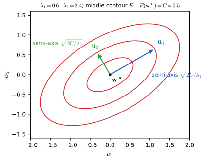
- If every \(\lambda_i>0\), the contour \(E-E(\bws)=C>0\) is an ellipsoid centred at \(\bws\) with axes along the \(\bu_i\) and semi-axis lengths \(\sqrt{2C/\lambda_i}\), inversely proportional to \(\sqrt{\lambda_i}\) (Figure 7.2).
Proof (Exercises 7.1, 7.2, 7.6)
(1) Substitute (7.10): \[(\bw-\bws)^\T\bH(\bw-\bws)=\sum_{i,j}\alpha_i\alpha_j\,\bu_i^\T\bH\bu_j.\] By (7.8), \(\bH\bu_j=\lambda_j\bu_j\), and by (7.9) \(\bu_i^\T\bu_j=\delta_{ij}\), so the double sum collapses to \(\sum_i\lambda_i\alpha_i^2\). Multiplying (7.10) on the left by \(\bu_j^\T\) gives \(\alpha_j=\bu_j^\T(\bw-\bws)\), which is (7.28) below.
(2) The same computation with \(c_i\) in place of \(\alpha_i\) gives (7.14). If all \(\lambda_i>0\) and \(\bv\ne\bzero\), some \(c_i\ne0\), so \(\sum_ic_i^2\lambda_i>0\). Conversely, if \(\bH\) is positive definite, taking \(\bv=\bu_i\) gives \(\lambda_i=\bu_i^\T\bH\bu_i>0\). The semi-definite case is identical with \(\ge\).
(3) The contour is \(\sum_i\lambda_i\alpha_i^2=2C\), i.e. \(\sum_i\alpha_i^2/(2C/\lambda_i)=1\): an ellipsoid in the rotated coordinates, whose \(i\)th semi-axis (set all other \(\alpha_j=0\)) has length \(\sqrt{2C/\lambda_i}\). The flattest direction (smallest \(\lambda_i\)) has the longest axis. ∎
The book concludes that "a necessary and sufficient condition" for \(\bws\) to be a local minimum is \(\nabla E(\bws)=\bzero\) with \(\bH\) positive definite. That is slightly too strong; the precise statement is:
Result 7.2 (second-order conditions for a minimum) p. 213; Exercise 7.3
Let \(E\) have continuous second derivatives near \(\bws\).
- Sufficient. If \(\nabla E(\bws)=\bzero\) and \(\bH(\bws)\) is positive definite, then \(\bws\) is a strict local minimum.
- Necessary. If \(\bws\) is a local minimum, then \(\nabla E(\bws)=\bzero\) and \(\bH(\bws)\) is positive semi-definite.
- Neither converse holds: \(E(w)=w^4\) has a strict minimum at 0 with \(H=0\) (not positive definite), and \(E(w)=w^3\) has \(E'(0)=0\), \(H=0\) (positive semi-definite) but no minimum. If some \(\lambda_i<0\), \(\bws\) is not a minimum; if all \(\lambda_i<0\), it is a strict local maximum; with both signs it is a saddle point.
For an exactly quadratic \(E\) such as (7.7), positive definiteness is necessary and sufficient for a strict (unique) minimum, which is the sense in which the book's statement is right.
Proof
Taylor's theorem with the Peano remainder: \[E(\bws+\bv)=E(\bws)+\bv^\T\nabla E(\bws)+\tfrac12\bv^\T\bH\bv+r(\bv)\] with \(r(\bv)/\|\bv\|^2\to0\) as \(\bv\to\bzero\).
(1) With \(\nabla E=\bzero\) and \(\lambda_{\min}>0\), (7.14) gives \(\tfrac12\bv^\T\bH\bv\ge\tfrac12\lambda_{\min}\|\bv\|^2\). Choose \(\rho>0\) with \(|r(\bv)|\le\tfrac14\lambda_{\min}\|\bv\|^2\) for \(\|\bv\|<\rho\). Then \[E(\bws+\bv)-E(\bws)\ge\tfrac14\lambda_{\min}\|\bv\|^2>0\] for \(0<\|\bv\|<\rho\).
(2) \(\nabla E=\bzero\) by Filling the gap 7.1. If some \(\lambda_i<0\), put \(\bv=\epsilon\bu_i\): \[E(\bws+\epsilon\bu_i)-E(\bws)=\tfrac12\lambda_i\epsilon^2+r(\epsilon\bu_i)<0\] for small \(\epsilon\ne0\), contradicting minimality. So all \(\lambda_i\ge0\).
(3) The examples are immediate. For a quadratic, \(r\equiv0\) and (7.11) shows that \(E>E(\bws)\) for all \(\bw\ne\bws\) iff all \(\lambda_i>0\). ∎
7.2 Gradient descent optimization
pp. 213–214 Solving \(\nabla E=\bzero\) analytically is hopeless for a neural network, so we iterate from an initial \(\bw^{(0)}\),
\[ \bw^{(\tau)}=\bw^{(\tau-1)}+\Delta\bw^{(\tau-1)}, \tag{7.15} \]with an update \(\Delta\bw\) that differs between algorithms. Because the error surface is not convex, the solution depends on \(\bw^{(0)}\); it can pay to run from several random starts and compare the results on a validation set.
7.2.1 Use of gradient information
See also the companion course, Section 5.2.3 and Filling the gap 5.4, where this counting argument is proved in full.
p. 214 The quadratic model (7.3) is fixed by \(\bb\) and the symmetric \(\bH\), \(W(W+3)/2\) numbers in all (Exercise 7.7). Without derivatives, each evaluation of \(E\) gives one number at cost \(O(W)\), so locating the minimum needs \(O(W^2)\) evaluations and \(O(W^3)\) operations. With the gradient, each evaluation gives \(W\) numbers at cost \(O(W)\) (by backpropagation), so \(O(W)\) evaluations suffice, \(O(W^2)\) operations in total.
Filling the gap 7.3: the count \(W(W+3)/2\), and what the \(O(W^2)\) estimate means p. 214; Exercise 7.7
Derivation
A symmetric \(W\times W\) matrix is determined by its \(W\) diagonal entries and the \(W(W-1)/2\) entries above the diagonal, \(W(W+1)/2\) numbers; adding the \(W\) entries of \(\bb\) gives \(W(W+1)/2+W=W(W+3)/2\). The minimiser of the quadratic is \(\widehat\bw-\bH^{-1}\bb\), which depends on all of them, so, information-theoretically, \(O(W^2)\) independent numbers have to be gathered.
The argument is a heuristic about information, not a theorem about a particular algorithm. It is made precise for quadratics by the conjugate-gradient method, which uses one gradient (\(W\) numbers) per step and reaches the exact minimiser of a positive definite quadratic in at most \(W\) steps in exact arithmetic: \(W\) gradients of cost \(O(W)\) each, \(O(W^2)\) operations, matching the estimate. Plain gradient descent does not achieve this: its number of steps depends on the condition number (Section 7.3), not on \(W\). ∎
7.2.2 Batch gradient descent
See also the companion course, Section 5.2.4 (gradient descent optimization).
p. 214 The simplest choice is a small step against the gradient,
\[ \bw^{(\tau)}=\bw^{(\tau-1)}-\eta\nabla E(\bw^{(\tau-1)}), \tag{7.16} \]with learning rate \(\eta>0\): gradient descent or steepest descent. Each step needs the gradient over the whole training set, which makes it a batch method. (Erratum. The book says the gradient is then "re-evaluated for the new weight vector \(\bw^{(\tau+1)}\)"; with the indexing of (7.16) it is \(\bw^{(\tau)}\).) How small must \(\eta\) be? For a smooth error there is a clean answer:
Result 7.3 (a small enough step always decreases the error) p. 214, (7.16)
Suppose \(\nabla E\) is \(L\)-Lipschitz, \[\|\nabla E(\bw)-\nabla E(\bw')\|\le L\|\bw-\bw'\|\] (for twice-differentiable \(E\) this holds with \(L=\sup\|\bH\|\), the largest \(|\lambda_i|\) over the region). Then one step of (7.16) satisfies
\[ E(\bw^{(\tau)})\le E(\bw^{(\tau-1)})-\eta\Big(1-\frac{L\eta}2\Big)\|\nabla E(\bw^{(\tau-1)})\|^2 . \]So for \(0<\eta<2/L\) every step lowers \(E\) unless the gradient is zero, and if \(E\ge E_{\inf}\),
\[ \min_{0\le\tau<T}\|\nabla E(\bw^{(\tau)})\|^2\le\frac{E(\bw^{(0)})-E_{\inf}}{T\,\eta\,(1-L\eta/2)}\ \longrightarrow\ 0 . \]For a quadratic \(L=\lambda_{\max}\), which is the bound \(\eta<2/\lambda_{\max}\) of Section 7.3.
Proof (the "descent lemma")
Write \(\bg=\nabla E(\bw)\) and \(\bw^+=\bw-\eta\bg\). By the fundamental theorem of calculus along the segment, \[E(\bw^+)-E(\bw)=\int_0^1\nabla E(\bw-t\eta\bg)^\T(-\eta\bg)\,\d t.\] Add and subtract \(\bg\): \[ E(\bw^+)-E(\bw)=-\eta\|\bg\|^2-\eta\int_0^1\big(\nabla E(\bw-t\eta\bg)-\bg\big)^\T\bg\,\d t\le-\eta\|\bg\|^2+\eta\int_0^1Lt\eta\|\bg\|^2\d t, \] using Cauchy–Schwarz and the Lipschitz bound \(\|\nabla E(\bw-t\eta\bg)-\bg\|\le Lt\eta\|\bg\|\). The integral is \(L\eta^2\|\bg\|^2/2\), which gives the inequality. Summing it over \(\tau=1,\dots,T\) telescopes the left side to at most \(E(\bw^{(0)})-E_{\inf}\), and the sum of \(T\) squared gradient norms is at least \(T\) times the smallest. ∎
Running logistic regression (where \(L=\lambda_{\max}(\bm X^\T\bm X)/4\)) with \(\eta=1.9/L\) confirms that \(E\) never increases.
7.2.3 Stochastic gradient descent
See also the companion course, Section 3.1.3 (sequential learning for least squares) and Section 5.2.4.
pp. 214–215 For independent observations the error is a sum over data points,
\[ E(\bw)=\sum_{n=1}^NE_n(\bw), \tag{7.17} \]and stochastic gradient descent (SGD, also on-line gradient descent) updates after each point,
\[ \bw^{(\tau)}=\bw^{(\tau-1)}-\eta\nabla E_n(\bw^{(\tau-1)}), \tag{7.18} \]cycling through the data; one pass is an epoch.
Algorithm 7.1 (stochastic gradient descent) p. 215
- Input: data indexed by \(n=1,\dots,N\), per-point errors \(E_n\), learning rate \(\eta\), initial \(\bw\). Set \(n\leftarrow1\).
- Repeat until convergence: \(\bw\leftarrow\bw-\eta\nabla E_n(\bw)\); \(n\leftarrow n+1\) (modulo \(N\)).
- Return \(\bw\).
Filling the gap 7.4: in what sense SGD follows the batch gradient, redundancy, and escaping stationary points p. 215
The book gives three informal arguments. Here they are made precise.
Derivation
Unbiasedness. If \(n\) is drawn uniformly from \(\{1,\dots,N\}\), then \[\E_n[\nabla E_n(\bw)]=\frac1N\sum_n\nabla E_n(\bw)=\frac1N\nabla E(\bw).\] So an SGD step is, on average, a batch step with learning rate \(\eta/N\), plus zero-mean noise. (With the mean error \(\bar E=E/N\), common in software, the SGD step has the same expected size as a batch step with the same \(\eta\).) Cycling through a shuffled data set gives the same expectation for each step.
Redundancy. Duplicate every point: \(E'(\bw)=2E(\bw)\), so \(\nabla E'=2\nabla E\), and batch descent on \(E'\) with rate \(\eta/2\) is identical to batch descent on \(E\) with rate \(\eta\), at twice the cost per step. One epoch of SGD on the duplicated data makes \(2N\) updates, each with the same distribution as an update on the original data: the information per update, and hence the progress per unit of computation, is unchanged.
Stationary points. At a stationary point of \(E\), \(\sum_n\nabla E_n(\bws)=\bzero\), but in general the individual \(\nabla E_n(\bws)\ne\bzero\) (their sum cancels, not each term). SGD steps therefore move away from \(\bws\) with a random direction whose covariance is that of the per-point gradients. Near a saddle point this pushes the iterate onto the direction of negative curvature, along which it then leaves at a geometric rate; near a minimum it makes the iterate fluctuate, which is why the learning rate must eventually decrease (Result 7.9). The optimiser demo, preset 5, shows both effects on a saddle. ∎
7.2.4 Mini-batches
pp. 216–217 A single-point gradient is a noisy estimate of the full gradient. A mini-batch of \(B\) points reduces the noise, with diminishing returns: the error of a mean of \(B\) samples falls only like \(\sigma/\sqrt B\) (Exercise 7.8). Points should be drawn at random (data sets are often ordered), usually by shuffling once per epoch and taking consecutive blocks.
Algorithm 7.2 (mini-batch stochastic gradient descent) p. 217
- Input: data \(n=1,\dots,N\), batch size \(B\), mini-batch error \(E_{n:n+B-1}\), learning rate \(\eta\), initial \(\bw\). Set \(n\leftarrow1\).
- Repeat until convergence: \(\bw\leftarrow\bw-\eta\nabla E_{n:n+B-1}(\bw)\); \(n\leftarrow n+B\); if \(n>N\), shuffle the data and set \(n\leftarrow1\).
- Return \(\bw\).
Result 7.4 (mean and variance of a mini-batch gradient) p. 216; Exercise 7.8
Fix \(\bw\). Let \(\bg_n=\nabla E_n(\bw)\), \(\bar\bg=\frac1N\sum_n\bg_n\) and \(\Sig=\frac1N\sum_n(\bg_n-\bar\bg)(\bg_n-\bar\bg)^\T\), with \(\sigma^2=\Tr\Sig\). For a mini-batch \(S\) of size \(B\) let \(\widehat\bg_B=\frac1B\sum_{n\in S}\bg_n\). Then \(\E[\widehat\bg_B]=\bar\bg\) and
\[ \cov[\widehat\bg_B]=\frac{\Sig}{B}\ \ \text{(with replacement)},\qquad \cov[\widehat\bg_B]=\frac{\Sig}{B}\,\frac{N-B}{N-1}\ \ \text{(without replacement)}. \]Hence \(\E\|\widehat\bg_B-\bar\bg\|^2=\sigma^2/B\) (times \((N-B)/(N-1)\) without replacement): the root-mean-square error falls like \(1/\sqrt B\), and vanishes at \(B=N\) without replacement.
Proof
With replacement. \(\widehat\bg_B\) is the mean of \(B\) independent draws \(\bg_{n_1},\dots,\bg_{n_B}\), each with mean \(\bar\bg\) and covariance \(\Sig\). Means are linear, and covariances of independent terms add: \(\cov[\frac1B\sum_k\bg_{n_k}]=\frac1{B^2}\cdot B\Sig\).
Without replacement. Write \(\widehat\bg_B-\bar\bg=\frac1B\sum_{n=1}^NI_n(\bg_n-\bar\bg)\) with \(I_n=1\) if \(n\in S\). For a uniformly random subset, \(\E[I_n]=B/N\), and for \(n\ne m\), \(\E[I_nI_m]=\frac{B(B-1)}{N(N-1)}\). Put \(\bm e_n=\bg_n-\bar\bg\), so \(\sum_n\bm e_n=\bzero\). Then \(\E[\widehat\bg_B]-\bar\bg=\frac1B\frac BN\sum_n\bm e_n=\bzero\), and \[ B^2\cov[\widehat\bg_B]=\frac BN\sum_n\bm e_n\bm e_n^\T+\frac{B(B-1)}{N(N-1)}\sum_{n\ne m}\bm e_n\bm e_m^\T . \] Since \[\sum_{n\ne m}\bm e_n\bm e_m^\T=(\sum_n\bm e_n)(\sum_m\bm e_m)^\T-\sum_n\bm e_n\bm e_n^\T=-N\Sig,\] this is \(B\Sig-\frac{B(B-1)}{N-1}\Sig=B\Sig\frac{N-B}{N-1}\). Divide by \(B^2\). Taking traces gives the scalar statements; Exercise 7.8 is the case of scalar data with replacement (independent samples). ∎
Numerical tests enumerate every subset of a population of 7 (\(B=2,3\)) and confirm both formulas exactly.
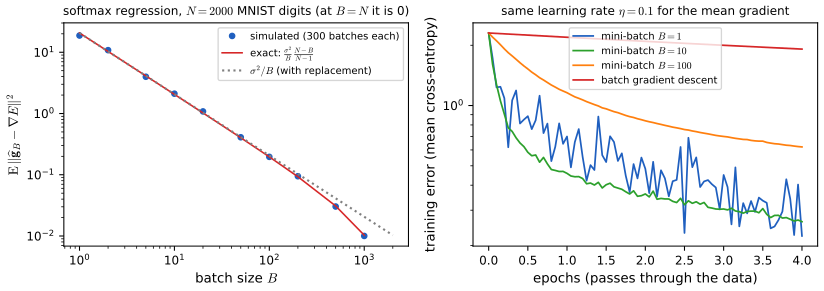
fig_7_s3. Download: PDF · SVG7.2.5 Parameter initialization
pp. 216–218 The starting point affects both the time to a solution and its generalisation. One requirement is clear: symmetry breaking. Units that receive the same inputs and start with the same parameters stay identical for ever, so the parameters are drawn at random, usually from a uniform distribution on \([-\epsilon,\epsilon]\) or from \(\N(0,\epsilon^2)\).
Filling the gap 7.5: identical units stay identical under gradient descent p. 216
Proof
Let hidden units \(j\) and \(k\) of a layer receive the same inputs, and suppose their incoming weights and biases are equal, and their outgoing weights are equal, at step \(\tau\). Swapping the two units (exchanging their incoming and their outgoing parameters) is a permutation \(P\) of weight space with \(E(P\bw)=E(\bw)\) for all \(\bw\) (it only reorders a sum). Differentiating, \(\nabla E(P\bw)=P\nabla E(\bw)\). At a fixed point of the swap, \(P\bw=\bw\), this gives \(\nabla E(\bw)=P\nabla E(\bw)\): the gradient is also unchanged by the swap, i.e. the two units receive identical updates. So \(P\bw^{(\tau+1)}=\bw^{(\tau+1)}\), and by induction the units remain identical forever (for any optimiser of Section 7.3 that acts the same way on every coordinate, since its state is then also swap-invariant). Setting all weights to zero is the extreme case. A random start has \(P\bw\ne\bw\) with probability one. Training a network started from identical hidden units confirms numerically that they stay equal to machine precision. ∎
The scale \(\epsilon\) matters. Consider layers computing
\[ a^{(l)}_i=\sum_{j=1}^Mw_{ij}z^{(l-1)}_j, \tag{7.19} \] \[ z^{(l)}_i=\ReLU(a^{(l)}_i), \tag{7.20} \]with weights drawn from \(\N(0,\epsilon^2)\). The book states (with \(\lambda^2\) "the variance of \(z^{(l-1)}_j\)")
\[ \E[a^{(l)}_i]=0, \tag{7.21} \] \[ \var[z^{(l)}_j]=\frac M2\epsilon^2\lambda^2 \quad\text{(as printed)}, \tag{7.22} \]and asks that the variance stay at \(\lambda^2\) from layer to layer, which gives He initialisation (He et al., 2015)
\[ \epsilon=\sqrt{\frac2M}. \tag{7.23} \]The conclusion (7.23) is right, but (7.22) as printed is not: its left side should be the variance of the pre-activation \(a^{(l)}_i\), and \(\lambda^2\) must be the variance of the previous pre-activation \(a^{(l-1)}\), not of the ReLU output \(z^{(l-1)}\). The precise statement and proof:
Result 7.5 (variance propagation at initialisation; He initialisation) pp. 217–218, (7.21)–(7.23); Exercise 7.9
Let the weights \(w_{ij}\) of layer \(l\) be independent \(\N(0,\epsilon^2)\) (any zero-mean symmetric distribution with variance \(\epsilon^2\) will do), independent of \(\bz^{(l-1)}\). Then
- \(\E[a^{(l)}_i]=0\) and \(\var[a^{(l)}_i]=M\epsilon^2\,\E\big[(z^{(l-1)}_j)^2\big]\) (a second moment of \(z\), not a variance).
- \(a^{(l)}_i\) is symmetric about 0, and for any symmetric \(a\), \(\E[\ReLU(a)^2]=\tfrac12\E[a^2]\). Therefore, when layer \(l-1\) is also of this form, \[ \var[a^{(l)}_i]=\frac M2\,\epsilon^2\,\var[a^{(l-1)}_i], \] which is (7.22) with \(a\) on the left and \(\lambda^2=\var[a^{(l-1)}]\) on the right. Keeping \(\var[a^{(l)}]\) constant requires \(\epsilon=\sqrt{2/M}\) (7.23).
- The variance of the ReLU output itself is different: for \(a\sim\N(0,\sigma^2)\), \(\E[\ReLU(a)]=\sigma/\sqrt{2\pi}\) and \[\var[\ReLU(a)]=\sigma^2\big(\tfrac12-\tfrac1{2\pi}\big)\approx0.341\,\sigma^2,\] not \(\sigma^2/2\). So (7.22) cannot be read literally.
- Backward pass. The backpropagated errors \(\delta^{(l)}_j=h'(a^{(l)}_j)\sum_iw_{ij}\delta^{(l+1)}_i\) (Chapter 8) obey, under the same independence assumptions, \(\var[\delta^{(l)}]=\tfrac12M_{\rm out}\epsilon^2\var[\delta^{(l+1)}]\) for ReLU, with \(M_{\rm out}\) the number of units fed by unit \(j\). With equal fan-in and fan-out, He initialisation keeps both directions stable.
Proof (Exercise 7.9, corrected)
(1) Each term \(w_{ij}z_j\) has \(\E[w_{ij}z_j]=\E[w_{ij}]\E[z_j]=0\) by independence, so \(\E[a_i]=0\). The terms are uncorrelated: for \(j\ne k\), \[\E[w_{ij}z_jw_{ik}z_k]=\E[w_{ij}]\E[w_{ik}]\E[z_jz_k]=0.\] Hence \[\var[a_i]=\sum_j\E[w_{ij}^2z_j^2]=\sum_j\epsilon^2\E[z_j^2]=M\epsilon^2\E[z^2],\] assuming the \(z_j\) have a common second moment.
(2) Symmetry. Conditional on \(\bz^{(l-1)}\), \(a_i=\sum_jw_{ij}z_j\) is a sum of independent symmetric variables (each \(w_{ij}\) is symmetric and \(z_j\) is fixed), hence symmetric; a mixture over \(\bz\) of symmetric laws is symmetric. The ReLU second moment. \(\ReLU(a)^2=a^2\,\mathbb 1\{a>0\}\). By symmetry \(\E[a^2\mathbb 1\{a>0\}]=\E[a^2\mathbb 1\{a<0\}]\), and the two add up to \(\E[a^2]\) (the event \(a=0\) contributes nothing), so each is \(\tfrac12\E[a^2]=\tfrac12\var[a]\) since \(\E[a]=0\). Combining with (1): \(\var[a^{(l)}]=M\epsilon^2\cdot\tfrac12\var[a^{(l-1)}]\). Setting the factor to 1 gives \(\epsilon^2=2/M\).
(3) For \(a\sim\N(0,\sigma^2)\): \[\E[\ReLU(a)]=\int_0^\infty a\,\frac{e^{-a^2/2\sigma^2}}{\sqrt{2\pi}\sigma}\d a=\frac{\sigma}{\sqrt{2\pi}},\] and \(\E[\ReLU(a)^2]=\sigma^2/2\) by (2), so \(\var=\sigma^2/2-\sigma^2/(2\pi)\).
(4) \(\delta^{(l)}_j=h'(a_j)\sum_iw_{ij}\delta^{(l+1)}_i\). Treating the weights \(w_{ij}\) as independent of the \(\delta^{(l+1)}_i\) (an approximation, since the same weights were used in the forward pass; it is the standard mean-field assumption, and simulation confirms its prediction) and \(h'(a_j)\in\{0,1\}\) with probability \(\tfrac12\) each, independent of the sum, the same computation as (1) gives \(\E[(\delta^{(l)}_j)^2]=\tfrac12\cdot M_{\rm out}\epsilon^2\,\E[(\delta^{(l+1)})^2]\). ∎
Other initialisations. For units that are linear near the origin (\(\tanh\), or no activation), \(h'(0)=1\) and there is no factor \(\tfrac12\): the forward pass needs \(\epsilon^2=1/M_{\rm in}\), the backward pass \(\epsilon^2=1/M_{\rm out}\), and Glorot and Bengio (2010) compromise on \(\epsilon^2=2/(M_{\rm in}+M_{\rm out})\). A uniform distribution on \([-\epsilon_U,\epsilon_U]\) has variance \(\epsilon_U^2/3\), so the uniform version of He initialisation uses \(\epsilon_U=\sqrt{6/M}\).
Numerical tests confirm (1)–(4) by Monte Carlo and on 8 random ReLU networks of 20 layers: the measured factor per layer is 1.03 forwards and 1.00 backwards for \(\epsilon^2=2/M\), and 0.51 and 0.50 for \(\epsilon^2=1/M\).
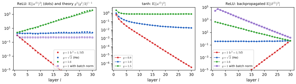
fig_7_s1. Download: PDF · SVGThe book adds that biases are often set to small positive values, so that most ReLU units start in their active region and receive a gradient, that the scale \(\epsilon\) can also be treated as a hyperparameter, and that a network can be initialised from one trained on another task (transfer learning, Section 6.3.4 of the book).
7.3 Convergence
See also the companion course, Result 5.13 (the same eigen-iteration, read as a filter that explains early stopping).
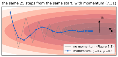
pp. 218–220 When the curvature differs strongly between directions, the error surface is a long valley (Figure 7.3). The negative gradient is perpendicular to the contours and points mostly across the valley, so the iterates zig-zag; increasing \(\eta\) speeds progress along the valley only until the oscillation across it diverges. The quadratic model makes this exact. From (7.7), (7.8) and (7.10),
\[ \nabla E=\sum_i\alpha_i\lambda_i\bu_i, \tag{7.24} \] \[ \Delta\bw=\sum_i\Delta\alpha_i\bu_i, \tag{7.25} \]and inserting both into the gradient descent step (7.16) and using (7.9),
\[ \Delta\alpha_i=-\eta\lambda_i\alpha_i, \tag{7.26} \] \[ \alpha_i^{\rm new}=(1-\eta\lambda_i)\alpha_i^{\rm old}, \tag{7.27} \] \[ \bu_i^\T(\bw-\bws)=\alpha_i, \tag{7.28} \] \[ \alpha_i^{(T)}=(1-\eta\lambda_i)^T\alpha_i^{(0)}. \tag{7.29} \]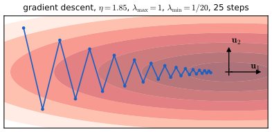
Definition 7.2 (condition number; linear convergence) pp. 219–220
For a positive definite Hessian, the condition number is \(\kappa=\lambda_{\max}/\lambda_{\min}\ge1\). A sequence converges linearly with rate \(\rho\in(0,1)\) if \(\|\bw^{(\tau)}-\bws\|\le C\rho^\tau\); the number of steps to reduce the error by a factor \(\varepsilon\) is then about \(\ln(1/\varepsilon)/\ln(1/\rho)\).
Result 7.6 (gradient descent on a quadratic) pp. 219–220, (7.24)–(7.30); Exercise 7.10
Let \(E\) be the quadratic (7.7) with \(\bH\) positive definite, eigenvalues \(0<\lambda_{\min}\le\dots\le\lambda_{\max}\).
- Gradient descent acts on each eigen-coordinate independently, (7.26)–(7.29), and \(\|\bw^{(T)}-\bws\|\le\rho(\eta)^T\|\bw^{(0)}-\bws\|\) with \[\rho(\eta)=\max_i|1-\eta\lambda_i|=\max(|1-\eta\lambda_{\min}|,|1-\eta\lambda_{\max}|).\]
- It converges from every starting point iff \(0<\eta<2/\lambda_{\max}\). At \(\eta=2/\lambda_{\max}\) exactly, the \(\lambda_{\max}\) coordinate flips sign for ever without shrinking.
- As \(\eta\uparrow2/\lambda_{\max}\), the slow coordinate contracts by \(1-2\lambda_{\min}/\lambda_{\max}\) per step, the factor (7.30) of the book: \[ \Big(1-\frac{2\lambda_{\min}}{\lambda_{\max}}\Big). \tag{7.30} \]
- The best fixed learning rate is \(\eta^\star=2/(\lambda_{\min}+\lambda_{\max})\), which gives \[ \rho(\eta^\star)=\frac{\lambda_{\max}-\lambda_{\min}}{\lambda_{\max}+\lambda_{\min}}=\frac{\kappa-1}{\kappa+1}, \] and about \(\frac\kappa2\ln(1/\varepsilon)\) steps to reduce the distance by \(\varepsilon\) when \(\kappa\) is large. The error itself, \(E-E(\bws)=\tfrac12\sum_i\lambda_i\alpha_i^2\), contracts by at least \(\rho^2\) per step.
Proof (Exercise 7.10 and the rest)
The iteration. Differentiating (7.7) gives \[\nabla E=\bH(\bw-\bws)=\sum_i\alpha_i\bH\bu_i=\sum_i\alpha_i\lambda_i\bu_i\] by (7.10) and (7.8): this is (7.24). Any change of \(\bw\) changes the coefficients of (7.10), \(\Delta\bw=\sum_i\Delta\alpha_i\bu_i\) (7.25). The step (7.16) says \(\sum_i\Delta\alpha_i\bu_i=-\eta\sum_i\alpha_i\lambda_i\bu_i\); multiply on the left by \(\bu_j^\T\) and use (7.9) to get \(\Delta\alpha_j=-\eta\lambda_j\alpha_j\) (7.26), i.e. (7.27); iterating gives (7.29).
(1) \(\|\bw-\bws\|^2=\sum_i\alpha_i^2\) (orthonormal coordinates), so \[\|\bw^{(T)}-\bws\|^2=\sum_i(1-\eta\lambda_i)^{2T}\alpha_i^{(0)2}\le\rho^{2T}\sum_i\alpha_i^{(0)2}.\] The function \(\lambda\mapsto|1-\eta\lambda|\) is convex, so its maximum over \([\lambda_{\min},\lambda_{\max}]\) is at an end point.
(2) \((1-\eta\lambda_i)^T\alpha_i^{(0)}\to0\) for every \(\alpha_i^{(0)}\) iff \(|1-\eta\lambda_i|<1\) iff \(0<\eta\lambda_i<2\). This must hold for every \(i\), i.e. \(\eta<2/\lambda_{\max}\). At equality \(1-\eta\lambda_{\max}=-1\).
(3) \(1-\eta\lambda_{\min}\to1-2\lambda_{\min}/\lambda_{\max}\). This is only the limit: at the bound itself (2) shows there is no convergence, and below it the \(\lambda_{\max}\) direction converges, but slowly when \(\eta\) is close to \(2/\lambda_{\max}\). The overall rate is therefore never (7.30) but \(\rho(\eta)\), which (4) optimises.
(4) \(|1-\eta\lambda_{\min}|=1-\eta\lambda_{\min}\) decreases and \(|1-\eta\lambda_{\max}|\) eventually increases in \(\eta\); the maximum of the two is smallest where they are equal, \(1-\eta\lambda_{\min}=\eta\lambda_{\max}-1\), i.e. \(\eta^\star=2/(\lambda_{\min}+\lambda_{\max})\), and then \[\rho=1-2\lambda_{\min}/(\lambda_{\min}+\lambda_{\max})=(\kappa-1)/(\kappa+1).\] Steps: \(\ln(1/\varepsilon)/\ln\frac{\kappa+1}{\kappa-1}\), and \(\ln\frac{\kappa+1}{\kappa-1}=\ln\frac{1+1/\kappa}{1-1/\kappa}=\frac2\kappa+O(\kappa^{-3})\). For the error, \(E-E(\bws)=\tfrac12\sum\lambda_i\alpha_i^2\) and each \(\alpha_i^2\) is multiplied by at most \(\rho^2\). ∎
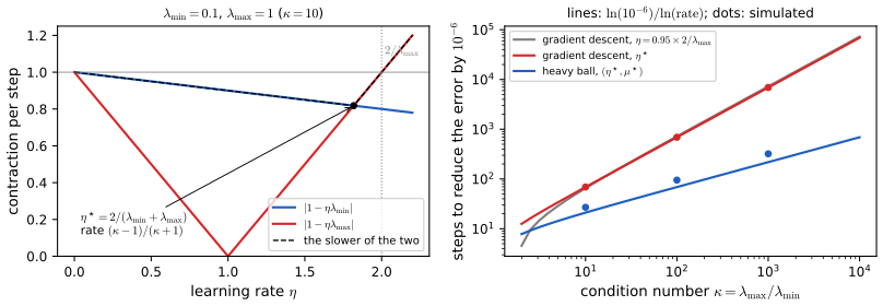
fig_7_s2. Download: PDF · SVGNote that (7.29) is linear convergence, that convergence requires every \(\lambda_i>0\) (so the stationary point is a minimum), and that the rate is governed by \(\kappa\): if \(\lambda_{\min}/\lambda_{\max}\) is tiny, progress along the valley floor is extremely slow.
7.3.1 Momentum
pp. 220–222 Adding a fraction of the previous step gives the update inertia:
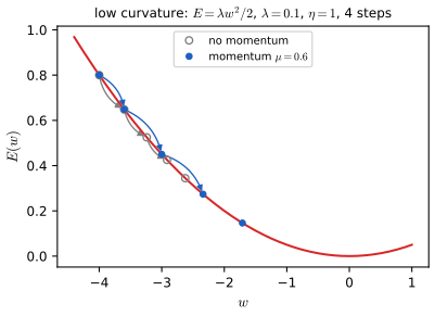
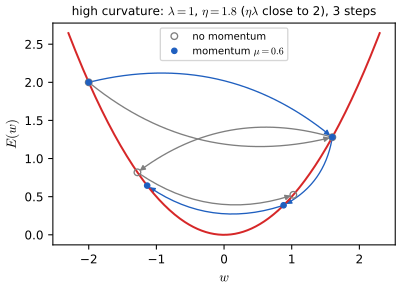
\[ \Delta\bw^{(\tau-1)}=-\eta\nabla E\big(\bw^{(\tau-1)}\big)+\mu\Delta\bw^{(\tau-2)}, \tag{7.31} \]followed by (7.15); \(\mu\) is the momentum parameter. If the gradient is nearly constant (a region of low curvature, Figure 7.4), repeated application gives a geometric series,
\[ \Delta\bw=-\eta\nabla E\{1+\mu+\mu^2+\dots\} \tag{7.32} \] \[ \phantom{\Delta\bw}=-\frac{\eta}{1-\mu}\nabla E, \tag{7.33} \]so the effective learning rate grows from \(\eta\) to \(\eta/(1-\mu)\), while in a region where gradient descent oscillates (Figure 7.5) successive contributions tend to cancel. A typical value is \(\mu=0.9\).
Filling the gap 7.6: the effective learning rate, exactly, and the range of \(\mu\) pp. 220–221, (7.32)–(7.33)
Derivation
Constant gradient. With \(\nabla E\equiv\bg\) and \(\Delta\bw^{(-1)}=\bzero\), (7.31) gives \(\Delta\bw^{(0)}=-\eta\bg\) and by induction \[\Delta\bw^{(k)}=-\eta\bg\sum_{j=0}^{k}\mu^j=-\eta\bg\,\frac{1-\mu^{k+1}}{1-\mu}.\] For \(|\mu|<1\) this tends to \(-\eta\bg/(1-\mu)\), (7.33), geometrically fast; after about \(1/(1-\mu)\) steps (10 steps for \(\mu=0.9\)) the step is within \(e^{-1}\) of its limit. For \(\mu=1\) the series diverges and the step grows without bound, so the admissible range is \(0\le\mu<1\), not \(0\le\mu\le1\) as the book writes.
Alternating gradient. If the gradient flips sign each step, \(\nabla E^{(k)}=(-1)^k\bg\), then \(\Delta\bw^{(k)}=-\eta\bg\sum_{j=0}^k(-1)^{k-j}\mu^j\), whose magnitude tends to \(\eta\|\bg\|/(1+\mu)\). So in an oscillating direction momentum reduces the effective rate to \(\eta/(1+\mu)\) (about \(\eta/1.9\) for \(\mu=0.9\)): "close to \(\eta\)" in the book is an understatement of the damping. Both limits are confirmed numerically.
A shift of scale. Since \(\eta/(1-\mu)\) is the effective step for slowly varying gradients, momentum \(\mu=0.9\) with rate \(\eta\) behaves, along the valley floor, like plain gradient descent with rate \(10\eta\); Figure 7.S4 shows exactly this on an MNIST network (momentum with \(\eta=0.01\) tracks plain SGD with \(\eta=0.1\)). The benefit is that across the valley the effective rate is only \(\eta/(1+\mu)\), so the oscillation that limits plain gradient descent does not appear. ∎
Algorithm 7.3 (stochastic gradient descent with momentum) p. 222
- Input: data, batch size \(B\), learning rate \(\eta\), momentum \(\mu\), initial \(\bw\). Set \(n\leftarrow1\), \(\Delta\bw\leftarrow\bzero\).
- Repeat until convergence: \(\Delta\bw\leftarrow-\eta\nabla E_{n:n+B-1}(\bw)+\mu\Delta\bw\); \(\bw\leftarrow\bw+\Delta\bw\); \(n\leftarrow n+B\); if \(n>N\), shuffle and set \(n\leftarrow1\).
- Return \(\bw\).
The book gives the intuition for momentum; on a quadratic the full answer is available, and it shows exactly how much momentum gains.
Result 7.7 (heavy-ball momentum on a quadratic) pp. 220–221, (7.31)
On the quadratic (7.7), momentum (7.31) acts on each eigen-coordinate separately through the two-term recursion
\[ \alpha_i^{(\tau+1)}=(1+\mu-\eta\lambda_i)\,\alpha_i^{(\tau)}-\mu\,\alpha_i^{(\tau-1)}, \]whose behaviour is governed by the roots of \(r^2-(1+\mu-\eta\lambda_i)r+\mu=0\). For \(0\le\mu<1\):
- both roots have modulus below 1 (convergence) iff \(0<\eta\lambda_i<2(1+\mu)\): momentum enlarges the stable range of \(\eta\) from \(2/\lambda_{\max}\) to \(2(1+\mu)/\lambda_{\max}\);
- when the roots are complex, i.e. \((1-\sqrt\mu)^2<\eta\lambda_i<(1+\sqrt\mu)^2\), both have modulus exactly \(\sqrt\mu\), whatever \(\lambda_i\);
- with Polyak's choice \[ \eta=\frac{4}{(\sqrt{\lambda_{\max}}+\sqrt{\lambda_{\min}})^2},\qquad \mu=\Big(\frac{\sqrt\kappa-1}{\sqrt\kappa+1}\Big)^2, \] every eigenvalue in \([\lambda_{\min},\lambda_{\max}]\) falls in the complex (or double-root) range, and the rate is \[ \sqrt\mu=\frac{\sqrt\kappa-1}{\sqrt\kappa+1}\approx1-\frac{2}{\sqrt\kappa}, \] so the number of steps is \(O(\sqrt\kappa)\) instead of \(O(\kappa)\): about 70 instead of 690 steps for \(\kappa=100\) and a reduction by \(10^6\).
Proof
The recursion. Project (7.31) on \(\bu_i\): with \(v^{(\tau)}=\alpha^{(\tau+1)}-\alpha^{(\tau)}\) the step in coordinate \(i\), \(v^{(\tau)}=-\eta\lambda_i\alpha^{(\tau)}+\mu v^{(\tau-1)}\). Substituting \(v^{(\tau-1)}=\alpha^{(\tau)}-\alpha^{(\tau-1)}\) gives the stated recursion. Its solutions are \(c_1r_1^\tau+c_2r_2^\tau\) (or \((c_1+c_2\tau)r^\tau\) for a double root) with \(r_{1,2}\) the roots of \(p(r)=r^2-Tr+\mu\), \(T=1+\mu-\eta\lambda_i\); so \(\alpha^{(\tau)}\to0\) for all starts iff both \(|r_k|<1\).
(2) Complex roots occur iff \(T^2<4\mu\), i.e. \(|1+\mu-\eta\lambda_i|<2\sqrt\mu\), i.e. \((1-\sqrt\mu)^2<\eta\lambda_i<(1+\sqrt\mu)^2\). Complex roots of a real polynomial are conjugate, so \(|r_1|^2=r_1\bar r_1=r_1r_2=\mu\).
(1) If the roots are complex, \(|r|=\sqrt\mu<1\), and \(|T|<2\sqrt\mu\le1+\mu\). If they are real: \(p(1)=1+\mu-T\) and \(p(-1)=1+\mu+T\). When \(|T|<1+\mu\) both are positive, and the vertex \(T/2\) lies in \((-1,1)\); a convex parabola that is positive at \(\pm1\) with its vertex between them has both roots in \((-1,1)\). When \(|T|\ge1+\mu\), \(p(1)\le0\) or \(p(-1)\le0\), and since \(p\to+\infty\) at \(\pm\infty\) there is a root with \(|r|\ge1\). So convergence iff \(|1+\mu-\eta\lambda_i|<1+\mu\), i.e. \(0<\eta\lambda_i<2(1+\mu)\).
(3) With \(s=\sqrt\kappa\) and \(\sqrt\mu=(s-1)/(s+1)\): \(1-\sqrt\mu=2/(s+1)\) and \(1+\sqrt\mu=2s/(s+1)\). With \[\eta=4/(\sqrt{\lambda_{\max}}+\sqrt{\lambda_{\min}})^2=4/(\lambda_{\min}(s+1)^2):\] \(\eta\lambda_{\min}=4/(s+1)^2=(1-\sqrt\mu)^2\) and \(\eta\lambda_{\max}=4s^2/(s+1)^2=(1+\sqrt\mu)^2\). So the end points sit exactly on the boundary of the complex range (double roots, modulus \(\sqrt\mu\)), and every \(\lambda\) in between gives complex roots of modulus \(\sqrt\mu\) by (2). Finally \(\ln\frac{s+1}{s-1}=\frac2s+O(s^{-3})\), so the step count is about \(\frac{\sqrt\kappa}2\ln(1/\varepsilon)\). Polyak (1964) shows that no other fixed \((\eta,\mu)\) does better on all quadratics with these eigenvalue bounds. ∎
Numerical tests: the stability boundary on both sides for 20 values of \(\mu\), the modulus \(\sqrt\mu\), and the spectral radius at Polyak's parameters for \(\kappa=10,100,1000\).
Nesterov momentum. In standard momentum the gradient is taken at the current point and the momentum step is added afterwards. Nesterov's variant (Nesterov 2004; Sutskever et al. 2013) first moves by the momentum and then takes the gradient there:
\[ \Delta\bw^{(\tau-1)}=-\eta\nabla E\big(\bw^{(\tau-1)}+\mu\Delta\bw^{(\tau-2)}\big)+\mu\Delta\bw^{(\tau-2)}. \tag{7.34} \]The book notes that it can improve the convergence of batch gradient descent but is less effective with stochastic gradients.
Result 7.8 (Nesterov momentum: the look-ahead form and a quadratic) p. 222, (7.34); Exercise 7.11
- With the look-ahead point \(\widetilde\bw^{(\tau)}=\bw^{(\tau)}+\mu\Delta\bw^{(\tau-1)}\) and \(\bm b=-\Delta\bw/\eta\), (7.34) is equivalent to \[ \bm b^{(\tau)}=\mu\bm b^{(\tau-1)}+\nabla E(\widetilde\bw^{(\tau)}),\qquad \widetilde\bw^{(\tau+1)}=\widetilde\bw^{(\tau)}-\eta\big(\nabla E(\widetilde\bw^{(\tau)})+\mu\bm b^{(\tau)}\big), \] which is how many software libraries implement it (the iterates they report are the look-ahead points).
- On the quadratic (7.7) each eigen-coordinate obeys \[ \alpha^{(\tau+1)}=(1+\mu)(1-\eta\lambda)\,\alpha^{(\tau)}-\mu(1-\eta\lambda)\,\alpha^{(\tau-1)}. \] With \(\eta=1/\lambda_{\max}\) and \(\mu=(\sqrt\kappa-1)/(\sqrt\kappa+1)\), every eigen-direction contracts at rate at most \(1-1/\sqrt\kappa\).
- (Exercise 7.11) For small \(\eta\) and \(\mu\) on a slowly varying surface, (7.34) and (7.31) differ by \(-\eta\mu\,\bH\Delta\bw^{(\tau-2)}+O(\eta\mu^2)\): a second-order quantity, so the two methods agree to first order.
Proof
(1) Write \(\bm v^{(\tau)}=\Delta\bw^{(\tau)}\) and \(\bg_\tau=\nabla E(\widetilde\bw^{(\tau)})\). By (7.34), \(\bm v^{(\tau)}=\mu\bm v^{(\tau-1)}-\eta\bg_\tau\), which with \(\bm b=-\bm v/\eta\) is the first equation. Then \[\widetilde\bw^{(\tau+1)}=\bw^{(\tau+1)}+\mu\bm v^{(\tau)}=\bw^{(\tau)}+(1+\mu)\bm v^{(\tau)}=\widetilde\bw^{(\tau)}-\mu\bm v^{(\tau-1)}+(1+\mu)\bm v^{(\tau)}.\] Substitute \(\mu\bm v^{(\tau-1)}=\bm v^{(\tau)}+\eta\bg_\tau\): \[\widetilde\bw^{(\tau+1)}=\widetilde\bw^{(\tau)}+\mu\bm v^{(\tau)}-\eta\bg_\tau=\widetilde\bw^{(\tau)}-\eta(\bg_\tau+\mu\bm b^{(\tau)}).\] A numerical test compares our (7.34) with the Nesterov option of a standard library step by step (difference \(2\times10^{-16}\)).
(2) In coordinate \(i\): \[v^{(\tau)}=\mu v^{(\tau-1)}-\eta\lambda(\alpha^{(\tau)}+\mu v^{(\tau-1)})=\mu(1-\eta\lambda)v^{(\tau-1)}-\eta\lambda\alpha^{(\tau)}.\] With \(v^{(\tau-1)}=\alpha^{(\tau)}-\alpha^{(\tau-1)}\) and \(\alpha^{(\tau+1)}=\alpha^{(\tau)}+v^{(\tau)}\) this is the stated recursion, with characteristic polynomial \(r^2-(1+\mu)q\,r+\mu q\), \(q=1-\eta\lambda\in[0,1-1/\kappa]\) for \(\eta=1/\lambda_{\max}\). Its discriminant is \(q\,[(1+\mu)^2q-4\mu]\). Put \(s=\sqrt\kappa\), \(\mu=(s-1)/(s+1)\), so \(1+\mu=2s/(s+1)\) and at \(\lambda=\lambda_{\min}\), \[q_{\min}=1-1/s^2=(s-1)(s+1)/s^2:\] then \[(1+\mu)^2q_{\min}=4(s-1)/(s+1)=4\mu,\] a double root \[r=(1+\mu)q_{\min}/2=(s-1)/s=1-1/s.\] For larger \(\lambda\), \(q<q_{\min}\), the discriminant is negative and \[|r|=\sqrt{\mu q}\le\sqrt{\mu q_{\min}}=\sqrt{\mu\cdot4\mu/(1+\mu)^2}=2\mu/(1+\mu)=1-1/s.\] At \(\lambda=\lambda_{\max}\), \(q=0\) and both roots are 0.
(3) Taylor-expand the gradient in (7.34): \[\nabla E(\bw+\mu\Delta\bw)=\nabla E(\bw)+\mu\bH\Delta\bw+O(\mu^2\|\Delta\bw\|^2).\] So (7.34) equals (7.31) plus \(-\eta\mu\bH\Delta\bw^{(\tau-2)}+O(\eta\mu^2)\). If \(\eta\) and \(\mu\) are both \(O(\epsilon)\) and the Hessian is bounded (slowly varying surface), the extra term is \(O(\epsilon^2)\) relative to the \(O(\epsilon)\) terms of (7.31). A numerical test shows that dividing \(\eta\) and \(\mu\) by 10 divides the difference by 100. ∎
7.3.2 Learning rate schedule
See also the companion course, Section 2.3.5 and Result 2.15 (the Robbins–Monro conditions, proved there for sequential estimation).
pp. 222–223 In practice one starts with a large learning rate and decreases it, \(\eta=\eta^{(\tau)}\):
\[ \bw^{(\tau)}=\bw^{(\tau-1)}-\eta^{(\tau-1)}\nabla E_n(\bw^{(\tau-1)}). \tag{7.35} \]Common schedules are linear, power-law and exponential decay:
\[ \eta^{(\tau)}=(1-\tau/K)\,\eta^{(0)}+(\tau/K)\,\eta^{(K)}, \tag{7.36} \] \[ \eta^{(\tau)}=\eta^{(0)}(1+\tau/s)^c, \tag{7.37} \] \[ \eta^{(\tau)}=\eta^{(0)}c^{\tau/s}, \tag{7.38} \]where (7.36) is held at \(\eta^{(K)}\) after \(K\) steps. Erratum. In (7.37) the exponent must be negative for a decay (write \((1+\tau/s)^{-c}\) with \(c>0\)); in (7.38) \(0<c<1\); and the text's list of hyperparameters calls \(s\) "\(S\)". Monitoring the learning curve helps to choose these values. Why decay at all? Because a constant learning rate with noisy gradients cannot converge:
Result 7.9 (the noise floor of constant-rate SGD, and the Robbins–Monro conditions) pp. 222–223
Take the one-dimensional quadratic \(E(w)=\lambda w^2/2\), \(\lambda>0\), and stochastic gradients \(g_\tau=\lambda w^{(\tau)}+\xi_\tau\) with independent noise, \(\E[\xi_\tau]=0\), \(\var[\xi_\tau]=s^2\) (a model of mini-batch noise near a minimum).
- With a constant rate \(0<\eta<2/\lambda\), \(\E[w^{(\tau)}]\to0\) but \(\E[(w^{(\tau)})^2]\to\dfrac{\eta s^2}{\lambda(2-\eta\lambda)}\approx\dfrac{\eta s^2}{2\lambda}\): the iterate keeps fluctuating, at a level proportional to \(\eta\).
- If \(\eta^{(\tau)}\to0\) with \(\sum_\tau\eta^{(\tau)}=\infty\) and \(\sum_\tau(\eta^{(\tau)})^2<\infty\) (the Robbins–Monro conditions), then \(\E[(w^{(\tau)})^2]\to0\). The power law \(\eta^{(0)}(1+\tau/s)^{-c}\) satisfies them for \(\tfrac12<c\le1\); the exponential schedule (7.38) does not (\(\sum\eta<\infty\)), so it can freeze before reaching the minimum; the linear schedule (7.36) ends at a constant \(\eta^{(K)}>0\) and so at the noise floor of (1).
Proof
The update is \(w^{(\tau+1)}=(1-\eta_\tau\lambda)w^{(\tau)}-\eta_\tau\xi_\tau\), with \(\xi_\tau\) independent of \(w^{(\tau)}\). Taking expectations, \(\E[w^{(\tau+1)}]=(1-\eta_\tau\lambda)\E[w^{(\tau)}]\). Squaring, the cross term has zero mean, so \(u_{\tau+1}=(1-\eta_\tau\lambda)^2u_\tau+\eta_\tau^2s^2\) for \(u_\tau=\E[(w^{(\tau)})^2]\).
(1) With constant \(\eta\) and \(|1-\eta\lambda|<1\) this linear recursion converges to its fixed point \[u^\star=\eta^2s^2/(1-(1-\eta\lambda)^2)=\eta^2s^2/(\eta\lambda(2-\eta\lambda)).\]
(2) Once \(\eta_\tau\lambda\le1\) (true for all large \(\tau\)), \((1-\eta_\tau\lambda)^2\le1-\eta_\tau\lambda\), so \(u_{\tau+1}\le(1-\eta_\tau\lambda)u_\tau+\eta_\tau^2s^2\). Unrolling from a large \(\tau_0\), \[ u_T\le u_{\tau_0}\prod_{\tau=\tau_0}^{T-1}(1-\eta_\tau\lambda)+s^2\sum_{k=\tau_0}^{T-1}\eta_k^2\prod_{\tau=k+1}^{T-1}(1-\eta_\tau\lambda). \] Since \(1-x\le e^{-x}\), the product is at most \(\exp(-\lambda\sum_{\tau=\tau_0}^{T-1}\eta_\tau)\to0\) because \(\sum\eta=\infty\). For the sum, given \(\varepsilon>0\) choose \(K\) with \(s^2\sum_{k\ge K}\eta_k^2<\varepsilon\) (possible since \(\sum\eta^2<\infty\)); the terms with \(k\ge K\) contribute less than \(\varepsilon\) (the products are at most 1), and the finitely many terms with \(k<K\) are each multiplied by a product that tends to 0. So \(\limsup u_T\le\varepsilon\) for every \(\varepsilon\). For the power law, \(\sum(1+\tau/s)^{-c}\) diverges iff \(c\le1\) and \(\sum(1+\tau/s)^{-2c}\) converges iff \(c>\tfrac12\). For (7.38), \(\sum_\tau c^{\tau/s}=1/(1-c^{1/s})<\infty\). ∎
Numerical tests: the noise floor (simulation, 20000 chains: 0.01316 against 0.01316), and the mean-square recursion with the power law (below \(10^{-5}\) after \(2\times10^5\) steps) and with the exponential schedule (frozen near \(9\times10^{-4}\)).
7.3.3 RMSProp and Adam
pp. 223–225 The best learning rate depends on the curvature, which differs between directions. This motivates a separate, automatically adapted learning rate for each weight. The book warns that the intuition really applies only when the principal curvature directions are aligned with the weight axes (a nearly diagonal Hessian). AdaGrad (Duchi, Hazan and Singer 2011) divides by the root of the accumulated squared derivatives,
\[ r_i^{(\tau)}=r_i^{(\tau-1)}+\Big(\frac{\partial E(\bw)}{\partial w_i}\Big)^2, \tag{7.39} \] \[ w_i^{(\tau)}=w_i^{(\tau-1)}-\frac{\eta}{\sqrt{r_i^{(\tau)}}+\delta}\Big(\frac{\partial E(\bw)}{\partial w_i}\Big), \tag{7.40} \]with \(r_i^{(0)}=0\), \(\delta\approx10^{-8}\), and \(E\) the mini-batch error. Because \(r_i\) only grows, the steps can become too small late in training. RMSProp (Hinton 2012) uses an exponentially weighted average instead,
\[ r_i^{(\tau)}=\beta r_i^{(\tau-1)}+(1-\beta)\Big(\frac{\partial E(\bw)}{\partial w_i}\Big)^2, \tag{7.41} \] \[ w_i^{(\tau)}=w_i^{(\tau-1)}-\frac{\eta}{\sqrt{r_i^{(\tau)}}+\delta}\Big(\frac{\partial E(\bw)}{\partial w_i}\Big), \tag{7.42} \]with \(0<\beta<1\), typically 0.9. Adam (Kingma and Ba 2014) combines this with momentum, keeping averages of the gradient and of its square,
\[ s_i^{(\tau)}=\beta_1s_i^{(\tau-1)}+(1-\beta_1)\Big(\frac{\partial E(\bw)}{\partial w_i}\Big), \tag{7.43} \] \[ r_i^{(\tau)}=\beta_2r_i^{(\tau-1)}+(1-\beta_2)\Big(\frac{\partial E(\bw)}{\partial w_i}\Big)^2, \tag{7.44} \] \[ \widehat s_i^{(\tau)}=\frac{s_i^{(\tau)}}{1-\beta_1^\tau}, \tag{7.45} \] \[ \widehat r_i^{(\tau)}=\frac{r_i^{(\tau)}}{1-\beta_2^\tau}, \tag{7.46} \] \[ w_i^{(\tau)}=w_i^{(\tau-1)}-\eta\,\frac{\widehat s_i^{(\tau)}}{\sqrt{\widehat r_i^{(\tau)}}+\delta}. \tag{7.47} \]The divisions by \(1-\beta^\tau\) correct the bias of starting the averages at zero (Exercise 7.12). The book quotes typical values \(\beta_1=0.9\), \(\beta_2=0.99\); Kingma and Ba recommend \(\beta_2=0.999\), the usual library default.
Algorithm 7.4 (Adam, with the sign corrected) p. 225
- Input: data, batch size \(B\), learning rate \(\eta\), decay rates \(\beta_1,\beta_2\), stabiliser \(\delta\), initial \(\bw\). Set \(\bm s\leftarrow\bzero\), \(\bm r\leftarrow\bzero\), \(\tau\leftarrow0\).
- Repeat until convergence: choose a mini-batch; \(\tau\leftarrow\tau+1\); \(\bg\leftarrow\nabla E_{\rm batch}(\bw)\); \(\bm s\leftarrow\beta_1\bm s+(1-\beta_1)\bg\); \(\bm r\leftarrow\beta_2\bm r+(1-\beta_2)\bg\odot\bg\); \(\widehat{\bm s}\leftarrow\bm s/(1-\beta_1^\tau)\); \(\widehat{\bm r}\leftarrow\bm r/(1-\beta_2^\tau)\); \(\Delta\bw\leftarrow-\eta\,\widehat{\bm s}/(\sqrt{\widehat{\bm r}}+\delta)\) elementwise; \(\bw\leftarrow\bw+\Delta\bw\).
- Return \(\bw\).
Erratum. The book's Algorithm 7.4 sets \(\bg=-\nabla E\) and then \(\Delta\bw\leftarrow-\eta\widehat{\bm s}/(\sqrt{\widehat{\bm r}}+\delta)\), \(\bw\leftarrow\bw+\Delta\bw\): with both minus signs the step is \(+\eta\nabla E/\ldots\), an ascent step. One of the two signs must go (here \(\bg=+\nabla E\), as in (7.43)). The algorithm also never increments the step counter \(\tau\) used in the bias corrections.
Result 7.10 (properties of the adaptive methods) pp. 223–225; Exercise 7.12
- Bias correction. Unrolling (7.43) from \(s^{(0)}=0\): \(s^{(\tau)}=(1-\beta_1)\sum_{k=1}^{\tau}\beta_1^{\tau-k}g_k\), whose weights sum to \(1-\beta_1^\tau\). So if the gradients have a common mean \(\bar g\), \(\E[s^{(\tau)}]=(1-\beta_1^\tau)\bar g\) and \(\widehat s^{(\tau)}\) is unbiased; the same holds for \(r\). The correction matters for \(\tau\lesssim1/(1-\beta)\) steps (10 for \(\beta_1=0.9\), 1000 for \(\beta_2=0.999\)).
- The first step is a sign step. At \(\tau=1\), \(\widehat s_i=g_i\) and \(\widehat r_i=g_i^2\), so \[\Delta w_i=-\eta g_i/(|g_i|+\delta)\approx-\eta\sign(g_i),\] whatever the size of the gradient.
- Scale invariance. Replacing \(E\) by \(cE\) (\(c>0\)) multiplies every \(s\) by \(c\) and every \(r\) by \(c^2\), so Adam and RMSProp take the same steps (up to \(\delta\)); the same holds coordinate by coordinate for a rescaling of each \(\partial E/\partial w_i\). Plain gradient descent would need \(\eta\to\eta/c\).
- Bounded steps. If \(\beta_1^2<\beta_2\), then for any sequence of gradients \[ \frac{|s_i^{(\tau)}|}{\sqrt{r_i^{(\tau)}}}\le\frac{1-\beta_1}{\sqrt{(1-\beta_2)(1-\beta_1^2/\beta_2)}}, \] so the raw step is at most a fixed multiple of \(\eta\) (7.3 for the default \(\beta\)'s): \(\eta\) sets the step length in weight space directly, unlike in gradient descent.
- Not rotation invariant. The per-coordinate scaling is tied to the weight axes. On a quadratic valley aligned with the axes it equalises the curvatures; on the same valley rotated by 45° it cannot.
Proof (Exercise 7.12 and the rest)
(1) Induction on (7.43) gives the unrolled sum (the same as (7.66) with \(\mu_0=0\)). Its weights are \((1-\beta)\beta^{\tau-k}\), \(k=1,\dots,\tau\), summing to \((1-\beta)\sum_{j=0}^{\tau-1}\beta^j=1-\beta^\tau\) by (7.67). Taking expectations term by term, \(\E[s^{(\tau)}]=(1-\beta^\tau)\bar g\); dividing by \(1-\beta^\tau\) removes the factor. If the mean of the gradients drifts, \(\widehat s\) is an average weighted towards recent values, not an unbiased estimate of the current mean. The time constant: \(\beta^\tau=e^{\tau\ln\beta}\approx e^{-\tau(1-\beta)}\).
(2) \(s^{(1)}=(1-\beta_1)g\), so \(\widehat s^{(1)}=g\); likewise \(\widehat r^{(1)}=g^2\) and \(\sqrt{\widehat r^{(1)}}=|g|\).
(3) Every \(s\) is linear in the gradients and every \(r\) quadratic, so \(\widehat s/\sqrt{\widehat r}\) is unchanged by \(g\to cg\); only \(\delta\) breaks the invariance, negligibly unless \(|g|\) is tiny.
(4) Drop the index \(i\). By the triangle inequality and then Cauchy–Schwarz with \[\beta_1^{\tau-k}|g_k|=(\beta_1/\sqrt{\beta_2})^{\tau-k}\cdot\sqrt{\beta_2}^{\,\tau-k}|g_k|:\] \[ |s^{(\tau)}|\le(1-\beta_1)\sum_k\beta_1^{\tau-k}|g_k|\le(1-\beta_1)\Big(\sum_k\gamma^{\tau-k}\Big)^{1/2}\Big(\sum_k\beta_2^{\tau-k}g_k^2\Big)^{1/2},\quad\gamma=\frac{\beta_1^2}{\beta_2}<1 . \] The first factor is at most \((1-\gamma)^{-1/2}\), and \(\sum_k\beta_2^{\tau-k}g_k^2=r^{(\tau)}/(1-\beta_2)\). Dividing by \(\sqrt{r^{(\tau)}}\) gives the bound. A numerical test feeds 200 adversarial sequences (heavy-tailed, and rare large spikes) and finds a largest ratio of 5.2 against the bound 7.3.
(5) Take \(E=\tfrac12(\lambda_1w_1^2+\lambda_2w_2^2)\). The gradient coordinates are \(\lambda_iw_i\), and \(\widehat s_i/\sqrt{\widehat r_i}\) does not depend on \(\lambda_i\) (by (3)), so both coordinates move at a speed set by \(\eta\) alone, as if the curvatures were equal. After a rotation each coordinate of the gradient mixes both curvatures and the rescaling can no longer separate them. ∎
Numerical tests also confirm that our implementations of (7.39)–(7.47) and of momentum agree step for step with a standard library's AdaGrad, RMSProp, Adam and SGD-with-momentum (differences \(\le6\times10^{-16}\)), and that Adam's path is unchanged when \(E\) is multiplied by 1000.
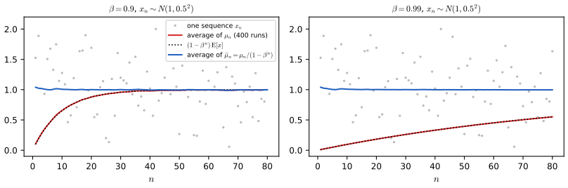
fig_7_s6. Download: PDF · SVG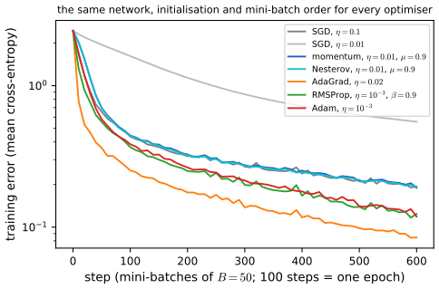
opt_update), with gradients from automatic differentiation. Code: fig_7_s4. Download: PDF · SVG7.4 Normalization
p. 224 Normalising the variables computed in the forward pass spares the network from handling very large or very small values. In principle weights and biases could adapt to any scale, but in practice normalisation can be crucial for effective training. There are three kinds, according to what is averaged over: the data set (inputs), the mini-batch, or the units of a layer.
7.4.1 Data normalization
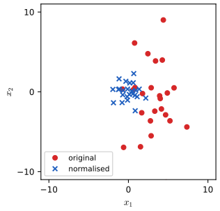
pp. 226 When input variables have very different ranges (height in metres, about 1.8; platelet count per microlitre, about 300,000), a change in one weight moves the output far more than the same change in another, so the error surface has very different curvatures along different axes, as in Figure 7.3. The remedy is to compute, once and before training,
\[ \mu_i=\frac1N\sum_{n=1}^Nx_{ni}, \tag{7.48} \] \[ \sigma_i^2=\frac1N\sum_{n=1}^N(x_{ni}-\mu_i)^2, \tag{7.49} \]and to train on
\[ \widetilde x_{ni}=\frac{x_{ni}-\mu_i}{\sigma_i}, \tag{7.50} \]which have zero mean and unit variance (Exercise 7.14). The same \(\mu_i\) and \(\sigma_i\), computed on the training set, must be used for validation and test data.
Filling the gap 7.7: what normalising the inputs does to the Hessian p. 226
The book's argument is qualitative. For a linear model it can be made exact.
Derivation
Take a linear output \(y=\bw^\T\bx+b\) with the sum-of-squares error. Its Hessian with respect to \((\bw,b)\) is the constant matrix \(\bH=\sum_n\widetilde{\bx}_n\widetilde{\bx}_n^\T\) with \(\widetilde{\bx}_n=(\bx_n,1)\) (Exercise 7.4 is the one-input case), independent of the targets and the weights. So by Section 7.3 gradient descent on this model converges at a rate fixed by the condition number of \(\bH\), which depends only on the inputs.
Centering decouples the bias. The off-diagonal block of \(\bH\) between \(\bw\) and \(b\) is \(\sum_n\bx_n=N\bm\mu\). After centring, \(\sum_n(\bx_n-\bm\mu)=\bzero\), so \(\bH=\begin{pmatrix}\bS&\bzero\\\bzero&N\end{pmatrix}\) with \(\bS=\sum_n(\bx_n-\bm\mu)(\bx_n-\bm\mu)^\T\): the bias becomes an independent direction.
Scaling equalises the diagonal. After (7.50), \(\bS/N\) is the correlation matrix \(\bm C\) of the inputs (unit diagonal) and \(\bH/N=\begin{pmatrix}\bm C&\bzero\\\bzero&1\end{pmatrix}\). Its eigenvalues are 1 and those of \(\bm C\), which lie in \([0,D]\) and average 1. For two inputs with correlation \(r\), the eigenvalues of \(\bm C\) are \(1\pm|r|\), so \(\kappa=(1+|r|)/(1-|r|)\), independent of the units of measurement. Before normalisation, with standard deviations differing by a factor \(F\), \(\kappa\) is of order \(F^2\) or larger. For the book's example (height in metres, sd about 0.1; platelets per microlitre, sd about 50,000) a numerical test finds \(\kappa\approx4\times10^{13}\) before and \(1.02\) after: gradient descent goes from hopeless to a handful of steps.
Correlations remain. Standardisation removes differences of scale, not correlations. Rotating to the principal components and scaling them (whitening) would make \(\bm C=\bI\) and \(\kappa=1\), at the price of mixing the input variables. ∎
7.4.2 Batch normalization
pp. 227–229 The same reasoning applies to hidden units, but their values change whenever the weights do, so the normalisation has to be repeated during training: this is batch normalisation (Ioffe and Szegedy 2015). A further motivation is the vanishing and exploding of gradients in deep networks. By the chain rule, the derivative with respect to a first-layer parameter is a product of one Jacobian per layer,
\[ \frac{\partial E}{\partial w_i}=\sum_m\cdots\sum_l\sum_j\frac{\partial z^{(1)}_m}{\partial w_i}\cdots\frac{\partial z^{(K)}_j}{\partial z^{(K-1)}_l}\frac{\partial E}{\partial z^{(K)}_j}, \tag{7.51} \]and a product of many factors tends to 0 if most of them are below 1 in magnitude and to \(\infty\) if most are above 1.
Filling the gap 7.8: how the product of Jacobians in (7.51) shrinks or grows p. 227, (7.51)
Derivation
In matrix form, (7.51) says \(\nabla_{\bz^{(1)}}E=\bJ_2^\T\bJ_3^\T\cdots\bJ_K^\T\nabla_{\bz^{(K)}}E\) with \[\bJ_k=\partial\bz^{(k)}/\partial\bz^{(k-1)}=\diag(h'(\ba^{(k)}))\bW^{(k)}.\] Submultiplicativity of the operator norm gives \(\|\nabla_{\bz^{(1)}}E\|\le\prod_k\|\bJ_k\|\cdot\|\nabla_{\bz^{(K)}}E\|\): if every \(\|\bJ_k\|\le q<1\) the gradient reaching the first layer is at most \(q^{K-1}\) times the output gradient (it vanishes exponentially in depth). The reverse bound does not hold for norms in general, but on average it does: for random weights as in Result 7.5 and a fixed vector \(\bv\), \(\E\|\bJ_k^\T\bv\|^2=M\epsilon^2\E[h'(a)^2]\|\bv\|^2\), so the squared gradient is multiplied on average by \(M\epsilon^2\E[h'(a)^2]\) per layer: \(g^2/2\) for ReLU with \(\epsilon=g/\sqrt M\). That factor is exactly 1 for He initialisation and \(1/2\) or \(1.62\) for \(g=1\) or \(g=1.8\), which after 20 layers means a factor \(2\times10^{-6}\) or \(10^4\) (Figure 7.S1, right). Initialisation can make the product right at the start of training; normalisation layers aim to keep it reasonable as the weights change. ∎
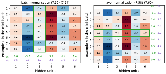
For a layer with pre-activations \(a_{ni}\) (example \(n\) of a mini-batch of size \(K\), unit \(i\)), batch normalisation computes
\[ \mu_i=\frac1K\sum_{n=1}^Ka_{ni}, \tag{7.52} \] \[ \sigma_i^2=\frac1K\sum_{n=1}^K(a_{ni}-\mu_i)^2, \tag{7.53} \] \[ \widehat a_{ni}=\frac{a_{ni}-\mu_i}{\sqrt{\sigma_i^2+\delta}}, \tag{7.54} \]with a small \(\delta\), and then restores a learnable mean and scale,
\[ \widetilde a_{ni}=\gamma_i\widehat a_{ni}+\beta_i . \tag{7.55} \]This does not simply undo the normalisation: the mean and standard deviation of the layer's output are now set directly by \(\beta_i\) and \(\gamma_i\) instead of by a complicated function of all the weights, which the book notes is much easier for gradient descent. The transformation is differentiable, so it is a layer like any other. At inference time there is no mini-batch, so running averages collected during training are used,
\[ \mu_i^{(\tau)}=\alpha\mu_i^{(\tau-1)}+(1-\alpha)\mu_i, \tag{7.56} \] \[ \sigma_i^{(\tau)}=\alpha\sigma_i^{(\tau-1)}+(1-\alpha)\sigma_i, \tag{7.57} \]with \(0\le\alpha\le1\). (These are exponentially weighted averages as in Exercise 7.12; if they start at zero they are biased towards zero for the first \(\approx1/(1-\alpha)\) steps, so implementations either start them at the first batch's values or train long enough.) Why batch normalisation works so well is not settled: it was motivated by "internal covariate shift", but Santurkar et al. (2018) argue that the gain comes from a smoother error landscape.
Backpropagation through (7.52)–(7.55) is not spelled out in the book. Because \(\mu_i\) and \(\sigma_i\) depend on every example of the batch, the derivative couples the examples:
Result 7.11 (gradients of batch and layer normalisation) pp. 227–229, (7.52)–(7.55), (7.58)–(7.60)
Fix a unit \(i\), write \(\widetilde\sigma_i=\sqrt{\sigma_i^2+\delta}\) and \(g_n=\partial E/\partial\widetilde a_{ni}\) (from the layers above). Then
\[ \frac{\partial E}{\partial\beta_i}=\sum_ng_n,\qquad\frac{\partial E}{\partial\gamma_i}=\sum_ng_n\widehat a_{ni}, \] \[ \frac{\partial E}{\partial a_{ni}}=\frac{\gamma_i}{\widetilde\sigma_i}\Big(g_n-\frac1K\sum_mg_m-\widehat a_{ni}\,\frac1K\sum_mg_m\widehat a_{mi}\Big). \]Consequently \(\sum_n\partial E/\partial a_{ni}=0\), and \(\sum_n\widehat a_{ni}\,\partial E/\partial a_{ni}=0\) when \(\delta=0\): the gradient with respect to the batch of pre-activations of a unit is projected away from the constant vector and from \(\widehat{\ba}_i\), the two directions along which the normalised output cannot change. Layer normalisation has the same formula with the roles of examples and units exchanged (means over the \(M\) units of example \(n\)).
Proof
The first two formulas follow from (7.55): \(\partial\widetilde a_{ni}/\partial\beta_i=1\) and \(\partial\widetilde a_{ni}/\partial\gamma_i=\widehat a_{ni}\), summed over the examples that share these parameters. For the third, drop \(i\), and let \(G_n=\partial E/\partial\widehat a_n=\gamma g_n\). From (7.52)–(7.54), \(\partial\mu/\partial a_m=1/K\) and \(\partial\sigma^2/\partial a_m=\frac2K(a_m-\mu)\) (the term from \(\partial\mu/\partial a_m\) is \(-\frac2K\sum_n(a_n-\mu)\cdot\frac1K=0\)). So \[ \frac{\partial\widehat a_n}{\partial a_m}=\frac{\delta_{nm}-1/K}{\widetilde\sigma}-\frac{a_n-\mu}{2\widetilde\sigma^3}\cdot\frac2K(a_m-\mu)=\frac1{\widetilde\sigma}\Big(\delta_{nm}-\frac1K-\frac1K\widehat a_n\widehat a_m\Big). \] Then \[\partial E/\partial a_m=\sum_nG_n\,\partial\widehat a_n/\partial a_m=\frac1{\widetilde\sigma}\big(G_m-\frac1K\sum_nG_n-\widehat a_m\frac1K\sum_nG_n\widehat a_n\big),\] the stated formula. Summing over \(m\) and using \(\sum_m\widehat a_m=0\) gives 0. Multiplying by \(\widehat a_m\) and summing, with \(\frac1K\sum_m\widehat a_m^2=\sigma^2/\widetilde\sigma^2\), gives \(\frac{1}{\widetilde\sigma}\sum_nG_n\widehat a_n\,(1-\sigma^2/\widetilde\sigma^2)\), which is 0 when \(\delta=0\). For layer normalisation the same computation runs over \(i=1,\dots,M\) for fixed \(n\). ∎
Numerical tests compare both formulas with automatic differentiation (agreement \(10^{-12}\)) and confirm the two orthogonality relations.
Filling the gap 7.9: scale invariance, and the learning rate that batch normalisation sets for itself pp. 228–229
The book says the learnable \(\gamma_i,\beta_i\) "turn out to be much easier to learn" than the statistics of an unnormalised layer. A concrete mechanism is an invariance.
Derivation
Invariance. Let \(a_{ni}=\bw_i^\T\bz_n+b_i\). Replacing \((\bw_i,b_i)\) by \((c\bw_i,cb_i+d)\) with \(c>0\) changes \(a_{ni}\to ca_{ni}+d\) for every \(n\), hence \(\mu_i\to c\mu_i+d\) and \(\sigma_i\to c\sigma_i\), and (with \(\delta=0\)) \(\widehat a_{ni}\) is unchanged. So the output of a batch-normalised layer does not depend on the length of \(\bw_i\) or on \(b_i\) at all: the bias is redundant (its role is taken by \(\beta_i\)) and only the direction of \(\bw_i\) matters.
Gradients. Differentiate \(E(c\bw_i)=E(\bw_i)\) with respect to \(c\) at \(c=1\): \(\bw_i^\T\nabla_{\bw_i}E=0\), the gradient is orthogonal to the weight vector. Differentiate \(E(c\bw)=E(\bw)\) with respect to \(\bw\): \(c\,\nabla E(c\bw)=\nabla E(\bw)\), so the gradient at \(c\bw\) is \(1/c\) times the gradient at \(\bw\).
Effective learning rate. A gradient step \(\bw_i\leftarrow\bw_i-\eta\nabla_{\bw_i}E\) is orthogonal to \(\bw_i\), so \(\|\bw_i\|^2\) can only grow: \[\|\bw_i-\eta\nabla E\|^2=\|\bw_i\|^2+\eta^2\|\nabla E\|^2.\] Since only the direction \(\bw_i/\|\bw_i\|\) matters, what counts is the angular step, \(\eta\|\nabla E(\bw_i)\|/\|\bw_i\|\), and by the \(1/c\) scaling this equals \(\eta\|\nabla E(\widehat\bw_i)\|/\|\bw_i\|^2\) with \(\widehat\bw_i\) the unit vector. So the effective learning rate on the direction is \(\eta/\|\bw_i\|^2\), and it automatically decreases as \(\|\bw_i\|\) grows: a large \(\eta\) causes large steps, which grow \(\|\bw_i\|\), which shrinks the effective rate. This self-stabilisation is one reason normalised networks tolerate a much wider range of learning rates (Figure 7.S5, right). ∎
Numerical tests confirm the invariance to per-unit scaling and shifts, the \(1/c\) scaling of the gradient, and its orthogonality to \(\bw_i\).
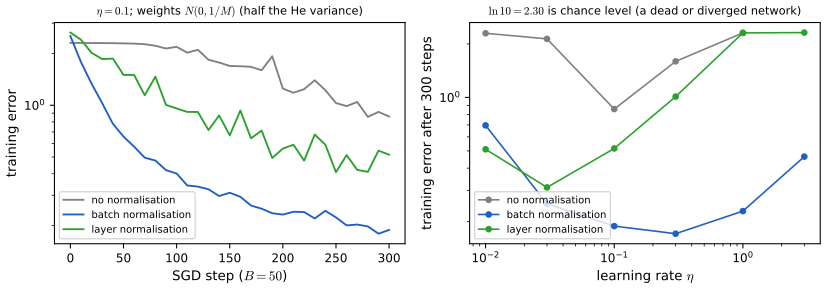
fig_7_s5. Download: PDF · SVG7.4.3 Layer normalization
pp. 229–230 With small mini-batches the batch statistics are noisy, and with batches split across devices they are expensive. Layer normalisation (Ba, Kiros and Hinton 2016), introduced for recurrent networks and now standard in transformers, normalises across the hidden units of each example instead:
\[ \mu_n=\frac1M\sum_{i=1}^Ma_{ni}, \tag{7.58} \] \[ \sigma_n^2=\frac1M\sum_{i=1}^M(a_{ni}-\mu_n)^2, \tag{7.59} \] \[ \widehat a_{ni}=\frac{a_{ni}-\mu_n}{\sqrt{\sigma_n^2+\delta}}, \tag{7.60} \]followed by learnable \(\gamma_i,\beta_i\) per unit as in (7.55). Erratum. The book prints \((a_{ni}-\mu_i)^2\) in (7.59); the mean subtracted is the example's own \(\mu_n\). The same computation is used in training and at inference, so no running averages are needed.
Filling the gap 7.10: what layer normalisation is invariant to, and how it differs from batch normalisation pp. 229–230
Derivation
Gradient. Result 7.11 with the sums over the \(M\) units of one example: \[\partial E/\partial a_{ni}=\frac1{\widetilde\sigma_n}\big(G_{ni}-\frac1M\sum_jG_{nj}-\widehat a_{ni}\frac1M\sum_jG_{nj}\widehat a_{nj}\big),\] \(G_{ni}=\gamma_ig_{ni}\). The examples are no longer coupled, which is why the output for one example does not depend on the rest of the batch (with batch normalisation it does, during training).
Invariances. If the whole weight matrix of the layer is scaled, \(\bW\to c\bW\) (\(c>0\)), and a common shift is added to all pre-activations of an example, then \(a_{ni}\to ca_{ni}+d_n\), \(\mu_n\to c\mu_n+d_n\), \(\sigma_n\to c\sigma_n\), and \(\widehat a_{ni}\) is unchanged (\(\delta=0\)). The same holds if the input \(\bz_n\) of the example is scaled. Batch normalisation is instead invariant to scaling each unit's weights separately (Filling the gap 7.9), and to scaling a feature across the whole batch, but not to rescaling a single example. So layer normalisation buys per-example independence at the price of treating the units of a layer as exchangeable: it assumes a common scale for all of them.
Numerical tests confirm the gradient formula against automatic differentiation and the invariance to \(\bW\to4\bW\) plus a shift. ∎
Summary: errors and imprecisions found in the chapter (first printing) and in the solutions manual
- (7.12): "for all \(\bv\)" must exclude \(\bv=\bzero\).
- Figure 7.2 caption: "square roots of the corresponding eigenvectors" should be eigenvalues.
- p. 213, Exercise 7.3: positive definiteness of \(\bH\) is sufficient for a (strict) local minimum but not necessary; the necessary condition is positive semi-definiteness (Result 7.2; \(E=w^4\) is a counterexample, checked numerically). The manual's solution of 7.3 proves the converse only for an exactly quadratic \(E\) and a strict minimum.
- p. 214: the gradient is re-evaluated at \(\bw^{(\tau)}\), not \(\bw^{(\tau+1)}\).
- (7.22): the left side should be \(\var[a^{(l)}_i]\) and \(\lambda^2\) the variance of the previous pre-activations; for ReLU outputs \(\var[z]=\sigma^2(\frac12-\frac1{2\pi})\ne\sigma^2/2\) (Result 7.5; Monte Carlo: 0.982 against \(\sigma^2/2=1.445\) for \(\sigma=1.7\)). The manual notes the left side (citing "(7.20)" where it means (7.22)) but then silently switches \(\lambda^2\) from the variance of \(z^{(l-1)}\) to that of \(a^{(l-1)}\), and writes \(\var[(a)^2]\) for \(\var[a]\).
- p. 221: the momentum parameter must satisfy \(0\le\mu<1\), not \(\le1\) (the series (7.32) diverges at \(\mu=1\)). In oscillating directions the effective rate is \(\eta/(1+\mu)\), not "close to \(\eta\)" (Filling the gap 7.6).
- (7.30): the factor holds only in the limit \(\eta\uparrow2/\lambda_{\max}\); at that value the \(\lambda_{\max}\) direction does not converge (checked), and the best overall rate is \((\kappa-1)/(\kappa+1)\) (Result 7.6).
- (7.37): the exponent must be negative for a decay; the text names the scale "\(S\)" instead of \(s\).
- Algorithm 7.4: with \(\bg=-\nabla E\) and \(\Delta\bw=-\eta\widehat{\bm s}/(\sqrt{\widehat{\bm r}}+\delta)\) the update ascends the error; the step counter \(\tau\) is never incremented.
- (7.59): \((a_{ni}-\mu_i)^2\) should be \((a_{ni}-\mu_n)^2\).
- (7.64), Exercise 7.5: the cross-entropy lacks its minus sign (as printed, the Hessian is negative definite; checked with autograd). The manual points this out.
- Manual, Solution 7.12: "which has the property \(\E[\mu_n]=\bar x\)" should read \(\E[\widehat\mu_n]\).
Exercises
All 14 exercises of Chapter 7 (Bishop and Bishop, 2024, pp. 230–232), restated in my own words, with complete solutions (hidden). Stars give the book's difficulty. Each was solved independently and then compared with the official solutions manual; where they differ, the solution says so and why.
Exercise 7.1 (★). Substitute the eigen-expansion (7.10) into the quadratic (7.7) and use (7.8) and (7.9) to obtain (7.11).
Solution
\[(\bw-\bws)^\T\bH(\bw-\bws)=\sum_{i,j}\alpha_i\alpha_j\bu_i^\T\bH\bu_j=\sum_{i,j}\alpha_i\alpha_j\lambda_j\bu_i^\T\bu_j=\sum_{i,j}\alpha_i\alpha_j\lambda_j\delta_{ij}=\sum_i\lambda_i\alpha_i^2.\] Inserting in (7.7) gives (7.11). (Result 7.1; same as the manual.)
Exercise 7.2 (★). Using (7.14) with \(\bv\) set to each eigenvector in turn, show that \(\bH\) is positive definite if and only if all its eigenvalues are positive.
Solution
If \(\bH\) is positive definite, \(\bv=\bu_i\ne\bzero\) gives \(0<\bu_i^\T\bH\bu_i=\lambda_i\). Conversely, if every \(\lambda_i>0\) and \(\bv=\sum_ic_i\bu_i\ne\bzero\), then some \(c_i\ne0\) and \(\bv^\T\bH\bv=\sum_ic_i^2\lambda_i>0\). The expansion exists because the eigenvectors of a symmetric matrix form an orthonormal basis. (Same as the manual.)
Exercise 7.3 (★★). Using the expansion (7.7) about a stationary point, show that \(\bws\) is a local minimum if and only if the Hessian there is positive definite.
Solution
Within the quadratic model (7.7), \(E(\bw)-E(\bws)=\tfrac12\sum_i\lambda_i\alpha_i^2\). If all \(\lambda_i>0\) this is positive for \(\bw\ne\bws\): a strict minimum. Conversely, if \(\bws\) is a strict minimum of (7.7), then taking \(\bw-\bws=\epsilon\bu_i\) gives \(\tfrac12\lambda_i\epsilon^2>0\), so \(\lambda_i>0\). For a general smooth \(E\) only half of this survives: positive definite is sufficient, and the necessary condition is positive semi-definite, since \(E=w^4\) has a strict minimum with \(H=0\) (Result 7.2, with the Taylor-remainder proof). Comparison. The manual's argument is the quadratic one and assumes \(E(\bw)>E(\bws)\) for all \(\bw\ne\bws\) (a strict and global minimum of the quadratic); it does not cover non-strict minima or the higher-order terms.
Exercise 7.4 (★★). For the model \(y=wx+b\) (7.61) with sum-of-squares error \(E=\tfrac12\sum_n(wx_n+b-t_n)^2\) (7.62), find the \(2\times2\) Hessian with respect to \((w,b)\) and show that its trace and determinant are positive, so the stationary point is a minimum.
Solution
\(\partial E/\partial w=\sum_n(y_n-t_n)x_n\), \(\partial E/\partial b=\sum_n(y_n-t_n)\). Differentiating again, \[ \bH=\begin{pmatrix}\sum_nx_n^2&\sum_nx_n\\\sum_nx_n&N\end{pmatrix}, \] independent of \(w,b\) and of the targets. \(\Tr\bH=\sum_nx_n^2+N>0\) and \[\det\bH=N\sum_nx_n^2-(\sum_nx_n)^2=N^2\sigma^2,\] with \(\sigma^2\) the (\(1/N\)) sample variance of the \(x_n\), which is positive unless all \(x_n\) are equal. A positive determinant means the eigenvalues have the same sign, and a positive trace means that sign is positive, so \(\bH\) is positive definite; as it is constant, \(E\) is strictly convex and the stationary point is the unique global minimum. A numerical test confirms \(\bH\) against automatic differentiation and \(\det\bH=N^2\sigma^2\). (Same as the manual. See also Section 3.1.1 of the companion course.)
Exercise 7.5 (★★). For \(y=\sigma(wx+b)\) (7.63) with the cross-entropy error (7.64), find the Hessian with respect to \((w,b)\) and show its trace and determinant are positive.
Solution
Erratum. (7.64) must read \[E=-\sum_n\{t_n\ln y_n+(1-t_n)\ln(1-y_n)\};\] without the minus sign the Hessian below changes sign and is negative definite (the manual notes this too). With \(\sigma'=\sigma(1-\sigma)\), \(\partial E/\partial w=\sum_n(y_n-t_n)x_n\) and \(\partial E/\partial b=\sum_n(y_n-t_n)\), and with \(c_n=y_n(1-y_n)\in(0,\tfrac14]\), \[ \bH=\begin{pmatrix}\sum_nc_nx_n^2&\sum_nc_nx_n\\\sum_nc_nx_n&\sum_nc_n\end{pmatrix}. \] \(\Tr\bH>0\) since every \(c_n>0\). With weights \(p_n=c_n/\sum_mc_m\) and weighted mean \(\bar x_c=\sum_np_nx_n\), \[\det\bH=(\sum_nc_n)^2\sum_np_n(x_n-\bar x_c)^2>0\] unless all \(x_n\) are equal. So \(\bH\) is positive definite at every \((w,b)\) and \(E\) is strictly convex. One caveat that the exercise (and the manual) pass over: strict convexity guarantees at most one stationary point, not that one exists. If the data are linearly separable, \(E\) decreases towards 0 as \(|w|\to\infty\) and has no minimiser at all. A numerical test confirms \(\bH\) against automatic differentiation, and that the printed sign gives a negative definite matrix. (See also Section 4.3.3 of the companion course.)
Exercise 7.6 (★★). Show that the contours of the quadratic (7.7) are ellipses with axes along the eigenvectors and semi-axis lengths inversely proportional to \(\sqrt{\lambda_i}\).
Solution
By (7.11), \(E=E(\bws)+C\) is \(\sum_i\lambda_i\alpha_i^2=2C\), i.e. \(\sum_i\alpha_i^2/a_i^2=1\) with \(a_i=\sqrt{2C/\lambda_i}\): an ellipse (ellipsoid for \(W>2\)) in the coordinates \(\alpha_i\), whose axes are the \(\bu_i\) directions, with semi-axis \(a_i\propto\lambda_i^{-1/2}\). This needs all \(\lambda_i>0\); with mixed signs the contours are hyperbolas. (Same as the manual; Figure 7.2 is drawn with exactly these lengths.)
Exercise 7.7 (★). Show that, because \(\bH\) is symmetric, the quadratic (7.3) has \(W(W+3)/2\) independent elements.
Solution
\(\bH\) has \(W\) diagonal entries and \((W^2-W)/2\) independent off-diagonal ones; \(\bb\) has \(W\). Total \(W+\frac{W(W-1)}2+W=\frac{W(W+3)}2\). (The constant \(E(\widehat\bw)\) does not affect the location of the minimum.) Same as the manual; see Filling the gap 7.3.
Exercise 7.8 (★). For independent \(x_1,\dots,x_N\) with mean \(\mu\) and variance \(\sigma^2\), and \(\bar x=\frac1N\sum_nx_n\) (7.65), show that \(\E[(\bar x-\mu)^2]=\sigma^2/N\).
Solution
\(\bar x-\mu=\frac1N\sum_n(x_n-\mu)\), so \[\E[(\bar x-\mu)^2]=\frac1{N^2}\sum_{n,m}\E[(x_n-\mu)(x_m-\mu)].\] Terms with \(n\ne m\) vanish by independence, those with \(n=m\) equal \(\sigma^2\): the result is \(N\sigma^2/N^2=\sigma^2/N\), and the RMS error is \(\sigma/\sqrt N\). Only uncorrelatedness is needed, not a Gaussian (the manual cites Gaussian properties, which is more than necessary). Sampling without replacement from a finite set gives the smaller value of Result 7.4. (See also Result 1.7 of the companion course.)
Exercise 7.9 (★★). For the layer (7.19)–(7.20) with weights \(\N(0,\epsilon^2)\), show (7.21) and (7.22), and deduce (7.23) by requiring the pre-activations of layer \(l\) to keep the variance \(\lambda^2\).
Solution
See Result 7.5: \(\E[a^{(l)}]=0\), \(\var[a^{(l)}]=M\epsilon^2\E[(z^{(l-1)})^2]\), and \(\E[\ReLU(a)^2]=\tfrac12\var[a]\) for symmetric \(a\), so \(\var[a^{(l)}]=\tfrac M2\epsilon^2\var[a^{(l-1)}]\); keeping it equal gives \(\epsilon=\sqrt{2/M}\). Comparison. As the manual notes, the left side of (7.22) should be \(\var[a^{(l)}_i]\) (the manual says "(7.20)", meaning (7.22)). The exercise also defines \(\lambda^2\) as the variance of the outputs \(z^{(l-1)}\), but the derivation needs \(\lambda^2=\var[a^{(l-1)}]\) (equivalently \(\E[(z^{(l-1)})^2]=\lambda^2/2\)); the manual makes this switch without comment, and its line "\(\tfrac12\var[(a)^2]\)" should be \(\tfrac12\var[a]\). If \(\lambda^2\) really were \(\var[z^{(l-1)}]\), the correct factor would involve \(\E[z^2]=\var[z]+\E[z]^2\), not \(\lambda^2/2\).
Exercise 7.10 (★★). Using (7.7), (7.8) and (7.10), derive the eigen-expansions (7.24) and (7.25), and with (7.9) and (7.16) derive (7.26).
Solution
See the first paragraph of the proof of Result 7.6: \(\nabla E=\bH(\bw-\bws)=\sum_i\alpha_i\lambda_i\bu_i\); \(\Delta\bw=\sum_i\Delta\alpha_i\bu_i\); equate with \(-\eta\nabla E\) and project on \(\bu_j\). (Same as the manual.)
Exercise 7.11 (★). On a slowly varying error surface, show that for small \(\eta\) and \(\mu\) Nesterov momentum (7.34) is equivalent to ordinary momentum (7.31).
Solution
\[\nabla E(\bw+\mu\Delta\bw)=\nabla E(\bw)+\mu\bH\Delta\bw+O(\mu^2),\] so (7.34) equals (7.31) plus \(-\eta\mu\bH\Delta\bw^{(\tau-2)}+O(\eta\mu^2)\), which is second order when \(\eta,\mu=O(\epsilon)\) and \(\bH=O(1)\). (Result 7.8(3); same as the manual. A numerical test finds the difference scales like \(\eta\mu\).)
Exercise 7.12 (★★). For the moving average \(\mu_n=\beta\mu_{n-1}+(1-\beta)x_n\) (7.66) with \(\mu_0=0\), use the geometric sum \(\sum_{k=1}^n\beta^{k-1}=(1-\beta^n)/(1-\beta)\) (7.67) to show that \(\mu_n\) is biased and that \[ \widehat\mu_n=\frac{\mu_n}{1-\beta^n} \tag{7.68} \] is not.
Solution
By induction, \[\mu_n=\beta^n\mu_0+(1-\beta)\sum_{k=1}^n\beta^{k-1}x_{n-k+1}.\] With \(\mu_0=0\) and \(\E[x_k]=\bar x\) for all \(k\), \[\E[\mu_n]=(1-\beta)\bar x\sum_{k=1}^n\beta^{k-1}=(1-\beta^n)\bar x\ne\bar x,\] and \(\E[\widehat\mu_n]=\bar x\). Only a common mean is needed (independence is not). Comparison. Same as the manual, whose last line should read \(\E[\widehat\mu_n]=\bar x\) (it writes \(\mu_n\)). (Result 7.10(1), Figure 7.S6; companion course: Section 2.3.5.)
Exercise 7.13 (★). In a line search, \(\lambda\) is chosen to minimise \(E(\bw^{(\tau)}+\lambda\bd)\) (7.69) along a direction \(\bd\). Show that the gradient at the new point is orthogonal to \(\bd\).
Solution
By the chain rule, \[\frac{\d}{\d\lambda}E(\bw^{(\tau)}+\lambda\bd)=\bd^\T\nabla E(\bw^{(\tau)}+\lambda\bd).\] At an interior minimiser \(\lambda^\star\) this derivative is zero, so \(\bd^\T\nabla E(\bw^{(\tau+1)})=0\). For steepest descent with exact line search (\(\bd=-\nabla E\)) successive search directions are therefore orthogonal, which produces the right-angled zig-zag in a long valley. For a quadratic the step is explicit, \(\lambda^\star=\bg^\T\bg/\bg^\T\bH\bg\) for \(\bd=-\bg\); a numerical test verifies the orthogonality. (Same as the manual.)
Exercise 7.14 (★). Show that the normalised inputs (7.50), with (7.48) and (7.49), have zero mean and unit variance.
Solution
\[\frac1N\sum_n\widetilde x_{ni}=\frac1{\sigma_i}\big(\frac1N\sum_nx_{ni}-\mu_i\big)=0,\] and then \[\frac1N\sum_n\widetilde x_{ni}^2=\frac1{\sigma_i^2}\frac1N\sum_n(x_{ni}-\mu_i)^2=1\] by (7.49). (With the \(1/N\) convention; the \(1/(N-1)\) variance would give \((N-1)/N\).) Same as the manual; a numerical test confirms it on the data of Figure 7.7.
Demonstrations
Three interactive pages, each linked above where its topic arises. They run in the browser and reproduce the Python code number for number (differences 0 for the paths, \(9\times10^{-16}\) relative for the depth statistics).
- Optimisers on a two-dimensional error surface: gradient descent, momentum, Nesterov, AdaGrad, RMSProp and Adam on a valley (any condition number and angle), a curved valley, two minima and a saddle; gradient noise and the schedules (7.36)–(7.38). Presets: 1 zig-zag (Fig 7.3), 2 momentum (Fig 7.6), 3 Adam on a rotated valley, 4 two minima (Fig 7.1), 5 saddle, noise and a schedule.
- Step size versus condition number: the eigen-coordinate iteration of Section 7.3, the contraction factors against \(\eta\), and the decay of each direction, for gradient descent, heavy ball and Nesterov. Presets: 1 just below \(2/\lambda_{\max}\), 2 divergence, 3 the best fixed step, 4 Polyak's momentum, 5 Nesterov at \(\kappa=1000\).
- Initialisation and activation statistics through depth: forward and backward statistics of a deep network at initialisation for any weight scale, ReLU, tanh or linear units, with batch or layer normalisation. Presets: 1 He, 2 variance 1/M, 3 exploding, 4 tanh saturation, 5 batch normalisation.
References
- Bishop, C. M. and Bishop, H. (2024). Deep Learning: Foundations and Concepts. Springer, Cham. Chapter 7, pp. 209–232. doi:10.1007/978-3-031-45468-4. Book website: www.bishopbook.com.
- Bishop, C. M. and Bishop, H. (2024). Deep Learning: Foundations and Concepts, Solutions to Exercises, version 1.0 (Chapters 2–10).
- Ba, J. L., Kiros, J. R. and Hinton, G. E. (2016). Layer normalization. arXiv:1607.06450.
- Bottou, L. (2010). Large-scale machine learning with stochastic gradient descent. In Proceedings of COMPSTAT 2010, 177–186. Physica-Verlag.
- Duchi, J., Hazan, E. and Singer, Y. (2011). Adaptive subgradient methods for online learning and stochastic optimization. Journal of Machine Learning Research, 12, 2121–2159.
- Glorot, X. and Bengio, Y. (2010). Understanding the difficulty of training deep feedforward neural networks. In Proceedings of the 13th International Conference on Artificial Intelligence and Statistics, 249–256.
- He, K., Zhang, X., Ren, S. and Sun, J. (2015). Delving deep into rectifiers: surpassing human-level performance on ImageNet classification. In Proceedings of the IEEE International Conference on Computer Vision, 1026–1034.
- Hinton, G. E. (2012). RMSProp: dividing the gradient by a running average of its recent magnitude. Lecture notes (cited by the book as Hinton, 2012).
- Ioffe, S. and Szegedy, C. (2015). Batch normalization: accelerating deep network training by reducing internal covariate shift. In Proceedings of the 32nd International Conference on Machine Learning, 448–456.
- Kingma, D. P. and Ba, J. (2014). Adam: a method for stochastic optimization. arXiv:1412.6980.
- Nesterov, Y. (2004). Introductory Lectures on Convex Optimization: A Basic Course. Kluwer Academic Publishers.
- Polyak, B. T. (1964). Some methods of speeding up the convergence of iteration methods. USSR Computational Mathematics and Mathematical Physics, 4(5), 1–17.
- Robbins, H. and Monro, S. (1951). A stochastic approximation method. The Annals of Mathematical Statistics, 22(3), 400–407. doi:10.1214/aoms/1177729586.
- Santurkar, S., Tsipras, D., Ilyas, A. and Madry, A. (2018). How does batch normalization help optimization? In Advances in Neural Information Processing Systems 31.
- Sutskever, I., Martens, J., Dahl, G. and Hinton, G. (2013). On the importance of initialization and momentum in deep learning. In Proceedings of the 30th International Conference on Machine Learning, 1139–1147.
- Yang, G., Pennington, J., Rao, V., Sohl-Dickstein, J. and Schoenholz, S. S. (2019). A mean field theory of batch normalization. In International Conference on Learning Representations.
Every numerical statement in these notes comes from ch07_gradient_descent.py; the MNIST experiments use the first 5000 training digits.