Graph learning
Graphs enter machine learning in two ways. Either the graph is the data, and we look for latent structure that explains it (communities, roles, a hierarchy of relations), or the graph is the unknown, and we infer it from correlated measurements (a tree, a directed acyclic graph, a sparse precision matrix, a causal diagram). The printed chapter is four pages long; the substance lives in the online supplement, which these notes follow section by section, proving the results the text states without proof and checking the numbers it quotes.
Ch. 1 Introduction Ch. 2 Probability Ch. 3 Statistics Ch. 4 Graphical models Ch. 5 Information theory Ch. 6 Optimisation Ch. 7 Inference algorithms Ch. 8 Gaussian filtering Ch. 9 Message passing Ch. 10 Variational inference Ch. 11 Monte Carlo Ch. 12 MCMC Ch. 13 Sequential Monte Carlo Ch. 14 Predictive models Ch. 15 GLMs Ch. 16 Deep networks Ch. 17 Bayesian neural networks Ch. 18 Gaussian processes Ch. 19 Beyond iid Ch. 20 Generative models Ch. 21 VAEs Ch. 22 Autoregressive models Ch. 23 Normalizing flows Ch. 24 Energy-based models Ch. 25 Diffusion models Ch. 26 GANs Ch. 27 Discovery methods Ch. 28 Latent factor models Ch. 29 State-space models Ch. 30 Graph learning Ch. 31 Nonparametric Bayes Ch. 32 Representation learning Ch. 33 Interpretability Ch. 34 Decision making Ch. 35 Reinforcement learning Ch. 36 Causality
How to read these notes
They follow the book. Sections carry the book's numbers. The online supplement has its own numbering (its Section 30.1 is the book's 30.2, its Sections 30.2 to 30.5 are the book's 30.3.1 and 30.3.2), so supplement sections are labelled supplement, written S30.k, and placed where the book points to them; supplement equations are written S(30.k) and keep their numbers. Equations without a number are steps the book skips.
Filling the gaps. Wherever the text says "one can show", quotes a result from the literature or leaves a step to the reader, an orange Filling the gap box gives the full argument. Proofs start hidden: open one with its bar, or use the buttons below. A few classical theorems (the converse of the Markov equivalence theorem, the Darmois-Skitovich theorem, the identifiability of nonlinear additive noise models) are quoted with a reference and checked numerically, and each says so.
Figures and demonstrations. Every computed figure is reproduced by the Python code, written from scratch. Figures that need data the book does not distribute (Sampson's monks, the college plans data, the relational data of the infinite relational model) are redone on simulations from the models of the text, and say so in the caption. Supplement figures are numbered S30.k; figures of my own are numbered x30.k.
Main reference
K. P. Murphy, Probabilistic Machine Learning: Advanced Topics, MIT Press (2023; online draft of December 2025), Chapter 30, pages 1043–1045 (book page: probml.github.io/pml-book/book2.html), and the supplementary material, Chapter 30, pages 227–266.
Companion courses
The probability behind this chapter is in Chapter 4 of this course (directed models and d-separation in Section 4.2, Gaussian MRFs in 4.3.5, the comparison of directed and undirected models in 4.5), with an elementary treatment in Bayesian ML Chapter 8 and All of Statistics Chapter 17 (DAGs) and Chapter 18 (undirected graphs, Gaussian graphical models). The lasso behind Section S30.4 is Volume 1, Section 11.4 (with the group lasso); independent component analysis, used for the non-Gaussian causal direction, is Section 28.6 of this course; graph embeddings and graph neural networks are Volume 1, Chapter 23.
What this chapter adds: why stochastic block models cannot be fitted by EM and how the collapsed sampler works, the Chow-Liu and matrix-tree theorems, the exact meaning of Markov equivalence and faithfulness, the Bayesian Dirichlet score and its likelihood equivalence, exact posteriors over all DAGs on five nodes, the correctness of the PC algorithm, the acyclicity constraint of NOTEARS, consistency of score-based search, three approximations to the marginal likelihood against the exact value, the graphical lasso derived from its optimality conditions, and the identifiability of cause and effect for pairs of variables.
The chapter at a glance
- S30.1 Stochastic block model: why EM fails, the collapsed likelihood, Gibbs sampling (gap 30.1); mixed membership and robust observation models (30.2); the Chinese restaurant process prior of the infinite relational model (30.3).
- S30.2 Trees: the Chow-Liu theorem (gap 30.4); maximum weight forests, mixtures of trees and the matrix-tree theorem (30.5).
- S30.3 DAGs: faithfulness (gap 30.6); Markov equivalence (30.7); the Dirichlet marginal likelihood and BDeu (30.8); counting DAGs and local search (30.9); the PC algorithm (30.10); NOTEARS (30.11); consistency (30.12); latent variables (30.13).
- S30.4 Undirected graphs: dependency networks and sparse Markov networks (gap 30.14); the Gaussian MLE and the graphical lasso (30.15).
- S30.5 Causal DAGs: cause-effect pairs (gap 30.16); information-geometric causal inference (30.17); interventional data (30.18).
Notation. A DAG \(G\) on nodes \(1,\dots,D\) has parent sets \(\pa(t)\); \(\bm x_t\) is the \(t\)-th variable, \(K_t\) its number of states, \(C_t\) the number of joint states of its parents. \(\bm S\) is a sample covariance, \(\bm\Omega=\bm\Sigma^{-1}\) a precision matrix, \(I(x_s;x_t)\) a mutual information in nats, \(x\indep y\given z\) conditional independence.
Prerequisites. Chapters 2, 4 and 5 of the book (conditional independence, graphical models, mutual information), the Dirichlet-multinomial model, and Volume 1, Section 11.4 (the lasso).
30.1 Introduction
p. 1043 A graph \(G\) is either observed and explained by latent variables (Section 30.2), or unknown and inferred from an \(N\times D\) data matrix whose columns it relates (Section 30.3). The first problem is unsupervised learning on a single large relational object (a social network, a protein interaction network); the second is model selection among graphical models, where the output has one node per variable, or extra latent nodes. Supervised learning on graph-structured inputs, by graph neural networks, is a different topic (Murphy 2023, Section 16.3.6; Volume 1, Chapter 23).
30.2 Latent variable models for graphs
p. 1043; Supplement S30.1, pp. 227–233 Given an observed graph, represented by an adjacency matrix \(\bm R\) with \(R_{ij}=1\) when node \(i\) links to node \(j\), we look for an "interesting structure" (communities, roles, a hierarchy of relations) and sometimes ask which links will form next. The models below put a discrete latent variable on every node and let the probability of a link depend only on the latent variables of its two ends. They are the graph analogue of a mixture model, with one decisive difference that Gap 30.1 explains.
S30.1.1 Stochastic block model supplement
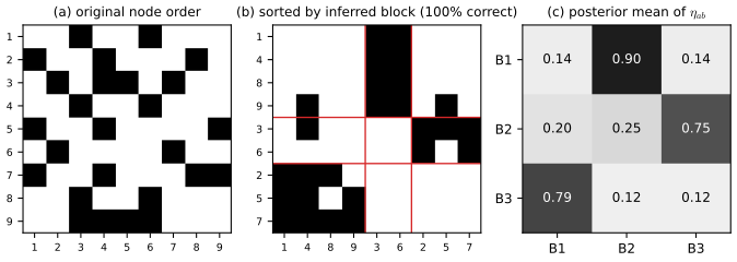
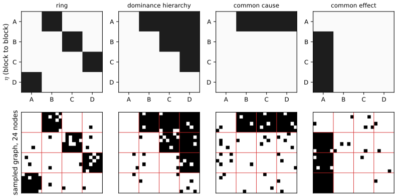
Supplement pp. 227–229 Each node \(i\) draws a block \(q_i\sim\Cat(\bm\pi)\); each ordered pair of blocks \((a,b)\) has a connection probability \(\eta_{ab}\) with a Beta prior; and every possible edge is an independent Bernoulli variable, \[ p(R_{ij}=r\given q_i=a,q_j=b,\bm\eta)=\Ber(r\given\eta_{ab}), \qquad i\ne j. \tag{S30.1} \] The blocks are not clusters of densely connected nodes: they are classes of nodes with the same connection profile. A block can have no edges inside it (the third block of Figure S30.2) as long as its members link to, and are linked from, the same other blocks. Choosing \(\bm\eta\) differently produces rings, dominance hierarchies, common-cause and common-effect structures (Figure S30.3), social networks of cliques, and so on. When the nodes carry features \(\bm x_i\), a discriminative version replaces the Bernoulli parameter by \(\Ber(\bm w_{ab}^{\T}f(\bm x_i,\bm x_j))\) (S(30.2)), a relational mixture of experts (Chapter 28 treats mixtures; the experts here are indexed by the pair of blocks).
Filling the gap 30.1: why EM fails, the collapsed likelihood and the Gibbs sampler Supplement p. 228, (S30.1)
Proof
(i) The posterior over blocks does not factorise. Given \(\bm\eta\) and \(\bm\pi\), \(p(\bm q\given\bm R)\propto\prod_i\pi_{q_i}\prod_{i\ne j}\eta_{q_iq_j}^{R_{ij}}(1-\eta_{q_iq_j})^{1-R_{ij}}\). Every pair \((i,j)\) contributes a factor depending on both \(q_i\) and \(q_j\), so the factor graph of the posterior is the complete graph on the nodes: there is no way to sum out one \(q_i\) without the others, and the E step of EM (which needs \(p(q_i\given\bm R)\), or pairwise marginals of a model that is a Markov random field with \(n\) fully connected variables) costs \(K^n\) in general. In a mixture model for iid data the factor graph is a set of disconnected stars (given the parameters the cases are independent), which is why exact EM works there. Approximations replace the E step: variational EM, or sampling.
(ii) Integrating out \(\bm\eta\). For a fixed labelling \(\bm q\), let \(m_{ab}=\sum_{i\ne j}R_{ij}\Ind[q_i=a,q_j=b]\) be the number of edges from block \(a\) to block \(b\) and \(t_{ab}=n_an_b-\delta_{ab}n_a\) the number of ordered pairs \(i\ne j\) in those blocks (\(n_a\) is the size of block \(a\)). The likelihood is \(\prod_{a,b}\eta_{ab}^{m_{ab}}(1-\eta_{ab})^{t_{ab}-m_{ab}}\). With independent \(\eta_{ab}\sim\mathrm{Beta}(\alpha_0,\beta_0)\) the integral factorises over block pairs and each factor is a Beta function, \[ p(\bm R\given\bm q)=\prod_{a,b}\frac{\Bt(\alpha_0+m_{ab},\,\beta_0+t_{ab}-m_{ab})}{\Bt(\alpha_0,\beta_0)},\qquad \Bt(u,v)=\int_0^1\eta^{u-1}(1-\eta)^{v-1}\d\eta. \] The posterior of \(\eta_{ab}\) given \(\bm q\) is \(\mathrm{Beta}(\alpha_0+m_{ab},\beta_0+t_{ab}-m_{ab})\), with mean \((\alpha_0+m_{ab})/(\alpha_0+\beta_0+t_{ab})\), the quantity shown in Figure S30.2(c).
(iii) Integrating out \(\bm\pi\). With \(\bm\pi\sim\Dir(\alpha,\dots,\alpha)\), \(p(\bm q)=\dfrac{\Gamma(K\alpha)}{\Gamma(K\alpha+n)}\prod_{k}\dfrac{\Gamma(\alpha+n_k)}{\Gamma(\alpha)}\) (the Dirichlet-multinomial marginal, gap 28.11).
(iv) Collapsed Gibbs sampling. The full conditional of one label is \(p(q_i=c\given\bm q_{-i},\bm R)\propto p(\bm q)\,p(\bm R\given\bm q)\) with \(q_i=c\), evaluated for \(c=1,\dots,K\) and normalised. Changing \(q_i\) only changes the counts in the row and column of \(i\), so with cached counts each candidate costs \(O(nK)\) (my code recomputes the whole product, which is fast enough for \(n\le 30\)). The sampler is a Markov chain on labellings whose stationary law is \(p(\bm q\given\bm R)\), which is what [Kem+06] use; [Air+08] use variational EM.
(v) Label switching. \(p(\bm R\given\bm q)p(\bm q)\) is unchanged if the labels are permuted, so the posterior has \(K!\) equivalent modes; estimates must be compared up to a permutation of the blocks (Figure S30.2 reports the accuracy under the best matching).
On the nine-node ring example of Figure S30.2 (three blocks of sizes 3, 4, 2, with \(\eta=0.9\) on the cycle of blocks and 0.1 elsewhere) the sampler recovers the blocks without error, and the posterior means of \(\eta\) are 0.90, 0.75 and 0.79 on the three ring entries, against 0.12–0.25 elsewhere. The collapsed likelihood agrees with a numerical integral over \(\eta\) and with a hand computation on a three-node graph.
See also. Section S28.1 (collapsed Gibbs sampling for topic models; the SBM sampler is the same idea), Bayesian ML Chapter 9 (EM for mixtures).
S30.1.2 Mixed membership stochastic block model supplement
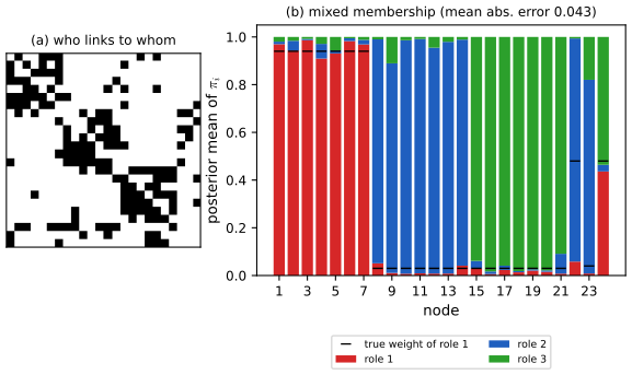
Supplement pp. 229–231 The mixed membership model replaces the hard label by a node-specific probability vector \(\bm\pi_i\sim\Dir(\alpha)\) in the simplex: node \(i\) plays role \(a\) with probability \(\pi_{ia}\), and may play a different role depending on whom it deals with. For every ordered pair a sending role and a receiving role are drawn, \[ q_{i\to j}\sim\Cat(\bm\pi_i),\quad q_{i\leftarrow j}\sim\Cat(\bm\pi_j),\quad p(R_{ij}=1\given q_{i\to j}=a,q_{i\leftarrow j}=b,\bm\eta)=\eta_{ab}. \tag{S30.3--S30.4} \] The vector \(\bm\pi_i\) expresses ontological uncertainty (to what degree node \(i\) belongs to each role); its posterior \(p(\bm\pi_i\given\bm R)\) expresses the separate epistemological uncertainty (what we do not know about the roles after seeing the data). Sampson's monks (a who-likes-whom matrix of 18 novices, collected by hand in 1968) are recovered as three groups with a few "waverers" of mixed membership; the data are not distributed with the book, so Figure S30.5 uses a network simulated from the model.
Filling the gap 30.2: the collapsed sampler for mixed membership, and what the robust observation model does Supplement pp. 229–231, S(30.3)–S(30.5)
Proof
(i) The marginal link probability. Averaging over the two role draws, \(p(R_{ij}=1\given\bm\pi_i,\bm\pi_j,\bm\eta)=\sum_{a,b}\pi_{ia}\pi_{jb}\eta_{ab}=\bm\pi_i^{\T}\bm\eta\bm\pi_j\): a bilinear form, so the model is a low-rank-like factorisation of the matrix of link probabilities, with soft memberships as factors. Pure memberships (\(\bm\pi_i\) a corner of the simplex) give the stochastic block model.
(ii) A collapsed Gibbs sampler. Take the state to be the pair of roles \((s_{ij},r_{ij})\) of every ordered pair, and integrate out \(\bm\pi_i\) and \(\bm\eta\). Let \(n_i[a]\) count how often node \(i\) plays role \(a\) over all roles drawn for it (as sender in its \(n-1\) pairs and as receiver in the other \(n-1\)), and \(m_{ab},t_{ab}\) the number of links and of pairs whose sending role is \(a\) and receiving role \(b\). Remove pair \((i,j)\) from the counts (denote the reduced counts by a minus superscript). By the Dirichlet-multinomial predictive and the Beta-Bernoulli predictive, \[ p\big(s_{ij}=a,r_{ij}=b\given\text{rest}\big)\;\propto\;\big(n^-_i[a]+\alpha\big)\big(n^-_j[b]+\alpha\big)\times\begin{cases}\dfrac{\alpha_0+m^-_{ab}}{\alpha_0+\beta_0+t^-_{ab}}&R_{ij}=1\\[2mm]\dfrac{\beta_0+t^-_{ab}-m^-_{ab}}{\alpha_0+\beta_0+t^-_{ab}}&R_{ij}=0.\end{cases} \] The two node factors are separate because \(i\ne j\) and each node's Dirichlet is collapsed on its own counts; the roles are drawn jointly from this table of \(K^2\) entries, then the counts are updated. The estimate of \(\bm\pi_i\) is the Gibbs average of \((n_i[a]+\alpha)/(\sum_{a'}n_i[a']+K\alpha)\), the Dirichlet posterior mean given the current roles.
(iii) Local optima and the check. Like all block models the posterior is multimodal, so the sampler is started at the hard labels of a spectral clustering (k-means on the leading eigenvectors of \(\bm R+\bm R^{\T}\)); on the 24-node network of Figure S30.5, with three pure groups of seven and three mixed members, the posterior mean recovers \(\bm\pi\) with mean absolute error 0.043. The three pure groups are classified correctly; the mixed members are only partly recovered (a node with 46 links carries little information about a mixture), which is the honest limit of the data.
(iv) The robust observation model. With probability \(\rho\) a pair is "background" and shows 0 whatever the roles, otherwise the link is \(\Ber(\eta_{ab})\) (S(30.5)). Then \(p(R_{ij}=1)=(1-\rho)\eta_{ab}\) and \(p(R_{ij}=0)=\rho+(1-\rho)(1-\eta_{ab})=1-(1-\rho)\eta_{ab}\). With \(\rho\) known this is the original model with the connection probability rescaled to \(\eta'_{ab}=(1-\rho)\eta_{ab}\); the effect is that a block density \(d\) is explained by \(\eta=d/(1-\rho)\), which must not exceed 1, so densities above \(1-\rho\) are impossible. The posterior probability that an observed 0 is a background (missing) one is \(\rho/\big(\rho+(1-\rho)(1-\eta_{ab})\big)\): near 1 when \(\eta_{ab}\) is near 1 (a missing link in a dense block is attributed to missing data, not to a real absence), near \(\rho\) when \(\eta_{ab}\) is small (a zero between sparse blocks is uninformative). An observed 1 always comes from the Bernoulli part.
S30.1.3 Infinite relational model supplement
Supplement pp. 231–233 The stochastic block model extends from graphs to relational data: a relation \(R(i,j,k)\) between entities of several types (for instance a ternary relation "adults \(i\), \(j\) are the parents of child \(k\)"). Every entity \(i\) of every type \(t\) gets a latent cluster \(q^t_i\), and the relation holds with the probability stored for the triple of clusters, \(p(R(i,j,k)=1\given q^1_i=a,q^1_j=b,q^2_k=c,\bm\eta)=\eta_{abc}\) (S(30.6)); real-valued relations use \(\N(\mu_{abc},\sigma^2)\), optionally with entity offsets (S(30.7)–S(30.8)). If the number of clusters of every type is unbounded and a Dirichlet process (or Chinese restaurant process) is the prior, the model is the infinite relational model (IRM, [Kem+06]; also the infinite hidden relational model [Xu+06]). Applied to the 135 concepts and 49 predicates of the Unified Medical Language System it finds 14 concept clusters and 21 predicate clusters (an ontology: biological functions affect organisms); applied to a 1965 political data set it clusters 14 countries, 54 interaction types and 90 features jointly, with relations treated as conditionally independent given the clusters, S(30.9). Both data sets are not distributed with the book and are not reproduced here.
Filling the gap 30.3: the Chinese restaurant process prior and its collapsed sampler Supplement pp. 231–233
Proof
(i) The prior. The Chinese restaurant process with concentration \(\alpha>0\) seats entity \(i\) at an existing table \(k\) with probability \(n_k/(i-1+\alpha)\) and at a new table with probability \(\alpha/(i-1+\alpha)\) (\(n_k\) are the current table sizes). Multiplying the seating probabilities of a given partition into \(K_+\) tables of final sizes \(n_1,\dots,n_{K_+}\): each table of size \(n_k\) contributes \(\alpha\cdot1\cdot2\cdots(n_k-1)\) to the numerator (the first customer opens the table, the \(r\)-th joining customer has \(r-1\) companions) and the denominators multiply to \(\alpha(\alpha+1)\cdots(\alpha+n-1)=\Gamma(\alpha+n)/\Gamma(\alpha)\), so \[ p(\bm q)=\frac{\Gamma(\alpha)}{\Gamma(\alpha+n)}\,\alpha^{K_+}\prod_{k=1}^{K_+}(n_k-1)!. \] This depends on the partition only, not on the order of the customers (exchangeability), and sums to 1 over the Bell number of set partitions (confirmed numerically for \(n=5\), 52 partitions). It is the limit \(K\to\infty\) of the finite Dirichlet-multinomial prior with \(\alpha/K\) pseudo counts.
(ii) The collapsed sampler. The Beta-Bernoulli integral of gap 30.1 applies to every triple of clusters (the counts \(m_{abc},t_{abc}\) now have three indices), giving \(p(\bm R\given\bm q)\) in closed form. By exchangeability any entity can be treated as the last one to be seated, so \(p(q_i=k\given\bm q_{-i},\bm R)\propto n_k^{-i}\,p(\bm R\given q_i=k,\bm q_{-i})\) for an existing cluster and \(\propto\alpha\,p(\bm R\given q_i=\text{new},\bm q_{-i})\) for a new one. Iterating over entities and relation types gives the sampler of [Kem+06]; the number of clusters is learned, and empty clusters disappear.
30.3 Graphical model structure learning
p. 1044 The input is an \(N\times D\) data matrix and the output a graph \(G\) (directed or undirected) with \(N_G\) nodes, usually \(N_G=D\), sometimes with extra latent nodes. The methods fall in a few families, and the supplement is organised by them.
30.3.1 Methods
p. 1044; Supplement Chapter 30 There are many methods for learning the structure of a probabilistic graphical model (see the review [VCB22] cited in the book). The supplement presents four groups:
- Trees (Section S30.2): the problem is easy, because the likelihood is a sum over edges and the best tree is a maximum weight spanning tree.
- DAGs (Section S30.3): scoring graphs by their marginal likelihood (Bayesian model selection), testing conditional independences (the PC algorithm), continuous optimisation with an acyclicity constraint, and the extra difficulties of hidden variables.
- Undirected graphs (Section S30.4): the likelihood does not decompose over the graph, so local search is expensive; one uses a product of full conditionals (dependency networks), the sparse Gaussian MLE (graphical lasso), group-lasso penalties for discrete variables, or Bayesian methods restricted to decomposable graphs.
- Causal discovery (Section S30.5): structure learning as a way to learn a structural causal model.
See also. Section 4.2.7 (learning the parameters of a directed model), 4.3.9 (learning undirected models, pseudo-likelihood), All of Statistics Section 17.6.
S30.2 Learning tree structures supplement
Supplement pp. 233–236 Searching all graphs is NP-hard ([Chi96]), so we start with trees, which can be learned efficiently and used for exact inference (Chapter 9). For an undirected tree \(T\) with edge set \(E(T)\) and pairwise potentials, the distribution is \[ p(\bm x\given T)=\prod_{t\in V}p(x_t)\prod_{(s,t)\in E(T)}\frac{p(x_s,x_t)}{p(x_s)p(x_t)}, \tag{S30.10} \] in terms of the node and edge marginals. For discrete variables the log-likelihood of data \(\mathcal D\) is, with counts \(N_{tk}\) and \(N_{stjk}\) (S(30.11)), \[ \log p(\mathcal D\given\bm\theta,T)=\sum_t\sum_kN_{tk}\log p(x_t=k)+\sum_{(s,t)\in E(T)}\sum_{j,k}N_{stjk}\log\frac{p(x_s=j,x_t=k)}{p(x_s=j)p(x_t=k)}. \]
S30.2.1 The Chow-Liu algorithm
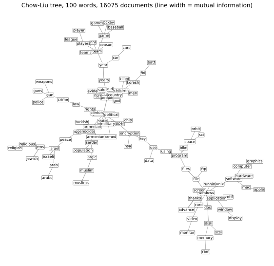
Setting the parameters to their maximum likelihood values (the empirical marginals \(\hat p\)), dividing by \(N\) gives \[ \frac1N\log p(\mathcal D\given\hat{\bm\theta},T)=-\sum_{t\in V}\Hent(\hat p_t)+\sum_{(s,t)\in E(T)}I(x_s;x_t\given\hat\theta_{st}), \tag{S30.12--S30.13} \] where \(I(x_s;x_t)=\sum_{j,k}\hat p(j,k)\log\frac{\hat p(j,k)}{\hat p(j)\hat p(k)}\ge0\) is the empirical mutual information (S(30.14)). The entropy term does not depend on \(T\), so the tree of maximum likelihood is the maximum weight spanning tree with weights \(I(x_s;x_t)\): the Chow-Liu algorithm [CL68]. Prim's and Kruskal's algorithms find it in \(O(E\log V)\) with \(E=D^2\); with the \(O(ND^2)\) cost of the mutual informations the total is \(O(ND^2+D^2\log D)\). Figure S30.8 shows the tree learned from binary bag-of-words data.
Filling the gap 30.4: the Chow-Liu theorem Supplement pp. 233–234, S(30.10)–S(30.14)
Proof
(i) (S30.10) is a normalised distribution. Root the tree at \(r\) and orient every edge away from it; let \(\pa(t)\) be the parent of \(t\ne r\). Then \(\prod_{(s,t)\in E}\frac{p(x_s,x_t)}{p(x_s)p(x_t)}=\prod_{t\ne r}\frac{p(x_t\given x_{\pa(t)})}{p(x_t)}\), so (S30.10) equals \(p(x_r)\prod_{t\ne r}p(x_t\given x_{\pa(t)})\): a directed model on a rooted tree, a product of normalised conditionals, hence normalised. It does not depend on the root. The marginals of this model on every node and every edge are the \(p(x_t)\) and \(p(x_s,x_t)\) used to build it (by summing the leaves out one at a time), so these are its parameters and (S30.10) is a faithful parametrisation of the tree model.
(ii) The MLE for a fixed tree. The log-likelihood of the rooted form is \(\sum_i\log p(x_{ir})+\sum_{t\ne r}\sum_i\log p(x_{it}\given x_{i,\pa(t)})\), a sum of terms each involving the separate free parameters of one family (the root marginal, and one conditional table for each other node). For one family, \(\sum_{j,k}N_{jk}\log\theta_{k\given j}\) is maximised, row by row under the constraint \(\sum_k\theta_{k\given j}=1\), by the empirical conditional \(N_{jk}/N_j\) (Gibbs' inequality: \(\sum_kp_k\log q_k\le\sum_kp_k\log p_k\)). Hence the maximised log-likelihood per case is \[ \frac1N\ell=-\Hent(\hat p_r)-\sum_{t\ne r}\Hent(\hat p_t\given\hat p_{\pa(t)}) \] in terms of empirical entropies, and conditional entropy is \(\Hent(x_t\given x_s)=\Hent(x_t)-I(x_s;x_t)\). Substituting gives \(-\sum_t\Hent(\hat p_t)+\sum_{t\ne r}I(x_{\pa(t)};x_t)\), the sum over the edges of the tree: (S30.12)–(S30.13). (Confirmed numerically: the direct likelihood and the entropy-plus-information formula agree to \(10^{-9}\) on the 100-word newsgroups data.)
(iii) Maximum weight spanning trees by Kruskal. Because every tree on \(D\) nodes has \(D-1\) edges and the same number of parameters, comparing maximised likelihoods across trees is fair, and the best tree maximises \(\sum_{E(T)}w_e\) with \(w_{st}=I(x_s;x_t)\). Cut property: for any partition of the nodes into two sets, the heaviest edge \(e\) crossing it lies in some maximum weight spanning tree. Indeed take a maximum tree \(T^*\) not containing \(e\); adding \(e\) closes a cycle, which crosses the cut at another edge \(f\in T^*\) with \(w_f\le w_e\); removing \(f\) leaves a spanning tree of weight at least \(w(T^*)\). Kruskal's algorithm scans the edges by decreasing weight and keeps an edge when it joins two different components; the edge it keeps is the heaviest one leaving the component of one end, so by the cut property (and induction on the edges kept) the result is a maximum weight spanning tree. The same argument with positive weights only gives gap 30.5. I confirmed numerically that Kruskal's tree has the same weight as scipy's, and that among all \(5^3=125\) labelled trees on five nodes the Chow-Liu tree has the largest likelihood.
(iv) Weights are non-negative, so the likelihood never prefers a forest. \(I\ge0\) (Gibbs' inequality again), so adding an edge never decreases the maximised likelihood; the maximum likelihood criterion never omits an edge (the next section changes this).
S30.2.2 Finding the MAP forest
Supplement pp. 234–235 If the marginal likelihood or a penalised likelihood replaces the likelihood, an optimal graph may be a forest. By the Dirichlet-multinomial marginal likelihood (gap 30.8), \(\log p(\mathcal D\given G)=\sum_t\mathrm{score}(\mathcal N_{t,\pa(t)})\) (S(30.15)). For graphs with at most one parent per node put \(w_{s,t}=\mathrm{score}(t\given s)-\mathrm{score}(t\given\emptyset)\), which may be negative; then \(\log p(\mathcal D\given T)=\sum_tw_{\pa(t),t}+\sum_t\mathrm{score}(t\given\emptyset)\) (S(30.16)), and finding the best forest is finding a maximal branching in a weighted directed graph [GGS84]. With a likelihood-equivalent score the weights are symmetric, \(\mathrm{score}(s\given t)+\mathrm{score}(t\given\emptyset)=\mathrm{score}(t\given s)+\mathrm{score}(s\given\emptyset)\) (S(30.17)), and then Kruskal's algorithm, run on the edges of positive weight only, gives the optimal forest.
S30.2.3 Mixtures of trees
Supplement pp. 235–236 A single tree is a weak model; a mixture of trees [MJ00] lets every component have its own tree, an unsupervised version of the tree-augmented naive Bayes classifier (Section 4.2.8). It is fitted by EM: the E step computes responsibilities, the M step runs a weighted version of Chow-Liu. Integrating over all trees gives an "infinite mixture of trees" in \(O(N_G^3)\) time through the matrix-tree theorem [MJ06].
Filling the gap 30.5: maximum weight forests, EM for mixtures of trees, and the matrix-tree theorem Supplement pp. 234–236
Proof
(i) Symmetry of the weights. For a family \((t\given s)\) with Dirichlet pseudo counts \(\alpha_{jk}\) on the joint states of \((x_s,x_t)\) whose marginals are \(\alpha_j=\sum_k\alpha_{jk}\), the product \(\mathrm{score}(s\given\emptyset)\,\mathrm{score}(t\given s)\) is, by the chain rule of the Dirichlet-multinomial, the marginal likelihood of the pair \((x_s,x_t)\) treated as one categorical variable with \(K_sK_t\) categories and Dirichlet prior \(\alpha_{jk}\) (the aggregation property of the Dirichlet: its marginal on \(x_s\) is \(\Dir(\alpha_j)\) and its conditionals on \(x_t\) given \(x_s=j\) are \(\Dir(\alpha_{j\cdot})\)). That expression is symmetric in \(s\) and \(t\) when the pseudo counts are; the BDeu prior \(\alpha/(K_sK_t)\) is (gap 30.8). Therefore \(w_{st}=\mathrm{score}(t\given s)-\mathrm{score}(t\given\emptyset)=\mathrm{score}(s\given t)-\mathrm{score}(s\given\emptyset)=w_{ts}\), which is (S30.17). I checked this numerically.
(ii) Optimal forest. A directed graph in which every node has at most one parent and no cycle is a branching, and it is an orientation of an undirected forest in which every component is rooted. Because \(w\) is symmetric, the total weight \(\sum_tw_{\pa(t),t}\) of a branching equals the weight of its underlying undirected forest, whichever roots are chosen; so the best branching has the weight of the best undirected forest. Removing an edge of negative weight raises the total, so the best forest uses only edges with \(w>0\). Let \(G'\) be the graph with the non-positive edges deleted; any forest of \(G'\) is a forest of \(G\), and a maximum weight forest of \(G'\) is a maximum weight spanning tree in each connected component of \(G'\) (a forest restricted to a component is a forest; adding weight is only possible by connecting that component). Running Kruskal on all positive-weight edges does exactly this without computing the components: the edges that join different components of the growing forest are the ones kept. (A brute-force search over all forests of six nodes with mixed signs agrees with this: checked.)
(iii) EM for a mixture of trees. With \(p(\bm x)=\sum_k\pi_kp(\bm x\given T_k,\bm\theta_k)\) the E step is \(r_{nk}\propto\pi_kp(\bm x_n\given T_k,\bm\theta_k)\) and the M step maximises \(\sum_{n,k}r_{nk}\log\big(\pi_kp(\bm x_n\given T_k,\bm\theta_k)\big)\). For each component this is the tree log-likelihood in which the data are weighted by \(r_{nk}\), so by gap 30.4 it is solved by the empirical marginals under weights \(r_{nk}/\sum_nr_{nk}\) and a maximum weight spanning tree of the \(r\)-weighted mutual informations, i.e. a weighted Chow-Liu step; \(\pi_k=\sum_nr_{nk}/N\). EM is monotone in the likelihood (Volume 1, gap 21.4).
(iv) The matrix-tree theorem. Put a weight \(w_e\ge0\) on every edge of the complete graph on \(n\) nodes and define the weight of a tree \(T\) by \(w(T)=\prod_{e\in T}w_e\) and \(Z=\sum_Tw(T)\) over all spanning trees. Then \(Z\) is the determinant of the weighted graph Laplacian \(\bm L=\diag(\bm W\bm 1)-\bm W\) with one row and the same column removed. Proof. Give every edge an arbitrary orientation and let \(\bm B\) be the \(n\times m\) incidence matrix (\(+1\) at the tail, \(-1\) at the head). Then \(\bm L=\bm B\diag(\bm w)\bm B^{\T}\). Let \(\bm B_r\) be \(\bm B\) with row \(r\) removed, so the reduced Laplacian is \(\bm L_r=\bm B_r\diag(\bm w)\bm B_r^{\T}\). The Cauchy-Binet formula for the product of an \((n-1)\times m\) and an \(m\times(n-1)\) matrix gives \(\det\bm L_r=\sum_{S}\det(\bm B_r[:,S])^2\prod_{e\in S}w_e\) over all sets \(S\) of \(n-1\) edges. If the edges of \(S\) contain a cycle, the corresponding columns of \(\bm B\) are linearly dependent (signed sum around the cycle is zero), hence so are those of \(\bm B_r\), and \(\det=0\). If \(S\) is a spanning tree, \(\det\bm B_r[:,S]=\pm1\): order the nodes so that a leaf other than \(r\) comes last, expand along its row (it has a single \(\pm1\)), and repeat on the smaller tree. Hence \(\det\bm L_r=\sum_Tw(T)=Z\).
(v) Edge marginals. Under \(p(T)=w(T)/Z\), \(\Pr(e\in T)=w_e\,\partial\log Z/\partial w_e\) (differentiate \(Z=\sum_T\prod w_e\): each tree containing \(e\) contributes its weight divided by \(w_e\)). By Jacobi's formula \(\partial\log\det\bm L_r=\Tr(\bm L_r^{-1}\partial\bm L_r)\), and \(\partial\bm L_r/\partial w_e=\bm b_e\bm b_e^{\T}\) with \(\bm b_e\) the column of \(\bm B_r\) of edge \(e\). Hence \(\Pr(e\in T)=w_e\,\bm b_e^{\T}\bm L_r^{-1}\bm b_e\), the weight times the effective resistance between the ends of \(e\) when edges are conductances \(w_e\). For an edge \((i,j)\) with neither end the removed node, \(\bm b_e^{\T}\bm L_r^{-1}\bm b_e=(\bm L_r^{-1})_{ii}+(\bm L_r^{-1})_{jj}-2(\bm L_r^{-1})_{ij}\); with the removed node as one end the first and cross terms are absent. All edge marginals cost one matrix inverse, \(O(n^3)\), which is the "exact Bayesian inference over all trees" of the supplement; they sum to \(n-1\). I verified (iv) and (v) against a sum over all 125 labelled trees on five nodes (Prüfer sequences).
S30.3 Learning DAG structures supplement
Supplement pp. 236–255 We estimate the structure of a directed model from observational data (Bayes net structure learning). This is only possible under the faithfulness assumption (S30.3.1), and the answer is only an equivalence class of DAGs, not a single graph (S30.3.2). If the DAG is read causally the same techniques give causal discovery, which needs further assumptions about confounding. See [GZS19].
S30.3.1 Faithfulness
Supplement p. 236 The Markov assumption lets us read conditional independences of \(p\) off a graph \(G\): every d-separation in \(G\) is a conditional independence of \(p\), \(I(G)\subseteq I(p)\). To go the other way we assume faithfulness (also called stability): \(I(p)=I(G)\), i.e. no conditional independence of \(p\) is due to a particular setting of parameters rather than to the graph. Consider the linear Gaussian model with independent errors \[ X=E_X,\quad Y=aX+E_Y,\quad Z=bY+cX+E_Z \tag{S30.18--S30.20} \] on the graph \(X\to Y\to Z\), \(X\to Z\). If \(ab+c=0\) then \(X\indep Z\), though the graph does not imply it. Such cancellations have probability zero when the coefficients are drawn from densities ([SGS00], Theorem 3.2).
Filling the gap 30.6: the cancellation, and why it has probability zero Supplement p. 236, S(30.18)–S(30.20)
Proof
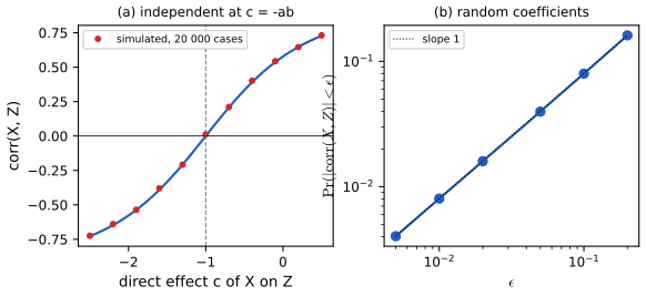
(i) The covariance. With \(\var(E_X)=\sigma_X^2\): \(Z=bY+cX+E_Z=(ab+c)X+bE_Y+E_Z\), and \(X\), \(E_Y\), \(E_Z\) are independent, so \(\cov(X,Z)=(ab+c)\sigma_X^2\) and \(\var(Z)=(ab+c)^2\sigma_X^2+b^2\sigma_Y^2+\sigma_Z^2\). For jointly Gaussian variables \(X\indep Z\) iff \(\cov(X,Z)=0\) iff \(ab+c=0\): the path \(X\to Y\to Z\) (effect \(ab\)) is exactly cancelled by the direct path (effect \(c\)). With \(\sigma\)'s equal to 1 the correlation is \(\rho=(ab+c)/\sqrt{(ab+c)^2+b^2+1}\) (Figure x30.1(a), simulated points on the curve).
(ii) Probability zero. The set \(\{(a,b,c):ab+c=0\}\) is the zero set of a non-zero polynomial, a surface in \(\R^3\), hence of Lebesgue measure zero; if \((a,b,c)\) has a density, \(\Pr(ab+c=0)=0\). More quantitatively, the density of \(\rho\) is positive and finite at 0 for random \((a,b,c)\), so \(\Pr(|\rho|<\epsilon)\) grows linearly in \(\epsilon\), and an approximate cancellation is as rare as the tolerance (Figure x30.1(b): slope 1 on the log-log plot, 400 000 draws of standard normal coefficients). For a general linear Gaussian DAG each partial correlation that the graph does not force to vanish is a ratio of polynomials in the parameters that is not identically zero, so the faithfulness violations lie in a finite union of proper algebraic sets, again of measure zero [SGS00]. Non-faithful distributions exist, but they are exceptional; they matter because a near-cancellation (small \(ab+c\)) makes the independence test fail at realistic sample sizes.
S30.3.2 Markov equivalence
Supplement pp. 237–238 Even with faithfulness a distribution does not identify its DAG. The three graphs \(X\to Y\to Z\), \(X\leftarrow Y\leftarrow Z\) and \(X\leftarrow Y\to Z\) all encode the same independences \(X\indep Z\given Y\), \(X\nindep Z\) (S(30.21)); they are Markov equivalent. The collider \(X\to Y\leftarrow Z\) encodes \(X\indep Z\), \(X\nindep Z\given Y\), a different model. Verma and Pearl (1990) proved:
Theorem S30.3.1. Two DAGs are Markov equivalent iff they have the same skeleton (the same edges, ignoring direction) and the same v-structures (colliders \(a\to c\leftarrow b\) with \(a,b\) not adjacent).
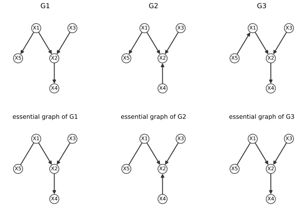
In Figure S30.10, \(G_1\not\equiv G_2\) because reversing \(2\to4\) creates a new v-structure, while \(G_1\equiv G_3\) because reversing \(1\to5\) does not. A class is represented by a partially directed graph, the PDAG (also essential graph or CPDAG), whose undirected edges are reversible and whose directed ones are compelled (Figure S30.11). One can learn a DAG only "up to Markov equivalence", even from infinite data, and one should not over-interpret individual edge directions.
Filling the gap 30.7: the Markov equivalence theorem, the covered-edge lemma and the essential graph Supplement pp. 237–238, Theorem S30.3.1
Proof
Write \(I(G)\) for the set of statements \(a\indep b\given S\) that hold in every distribution Markov to \(G\) (d-separations). \(G\) and \(H\) are equivalent when \(I(G)=I(H)\).
(i) Equivalent graphs have the same skeleton. If \(a,b\) are adjacent in \(G\), no \(S\) d-separates them (the edge is an active path without intermediate nodes). If they are not adjacent, one is not a descendant of the other, say \(b\) is not a descendant of \(a\); by the local Markov property \(a\indep b\given\pa(a)\) (a node is independent of its non-descendants given its parents, and \(b\notin\pa(a)\)), so some \(S\) separates them. Hence adjacency is the property "no separating set exists", which is read off \(I(G)\).
(ii) Equivalent graphs have the same v-structures. Let \(a\to c\leftarrow b\) be a v-structure of \(G\). Any set \(S\) separating \(a,b\) in \(G\) (one exists by (i)) must exclude \(c\) and all its descendants: otherwise the path \(a\to c\leftarrow b\) would be active. Suppose \(H\) has the same skeleton but \(c\) is not a collider on \(a - c - b\) in \(H\). Then this path is blocked only by conditioning on \(c\), so every separating set of \(H\) contains \(c\). Since \(I(G)=I(H)\), a set that separates \(a,b\) in \(G\) and excludes \(c\) also separates them in \(H\), a contradiction. So \(a\to c\leftarrow b\) is a v-structure of \(H\) as well (and \(a,b\) are non-adjacent in both). This proves "only if".
(iii) The converse. For "if", I use the lemma below and quote a theorem of graph theory. Covered edge lemma. An edge \(x\to y\) of a DAG is covered if \(\pa(y)=\pa(x)\cup\{x\}\). Let \(Z=\pa(x)\) and let \(H\) be \(G\) with \(x\to y\) reversed. A distribution factorises on \(G\) as \(\prod_{v}p(v\given\pa(v))\) in which the factors of \(x\) and \(y\) are \(p(x\given\bm z)\,p(y\given\bm z,x)=p(x,y\given\bm z)=p(y\given\bm z)\,p(x\given\bm z,y)\); the right side is the pair of factors for \(H\), where \(\pa_H(y)=Z\) and \(\pa_H(x)=Z\cup\{y\}\). All other nodes have the same parents in \(G\) and \(H\) (only the children lists of \(x,y\) change, and no other parent set contains \(x\) or \(y\) differently). So the two models contain exactly the same distributions, hence the same independences, and the same likelihood and (see gap 30.8) the same BDeu score. Chickering's theorem (1995): two DAGs have the same skeleton and v-structures iff one can be turned into the other by a sequence of covered edge reversals. Together with the lemma this gives the "if" of Theorem S30.3.1. I did not reprove Chickering's theorem; instead I checked the whole statement by brute force: for each of the 543 DAGs on four nodes I computed the set of all d-separation statements, and two DAGs have the same set exactly when they have the same skeleton and v-structures. There are 185 classes on four nodes and 8782 on five (1, 2, 11, 185, 8782 for 1 to 5 nodes), found by grouping the 29 281 five-node DAGs; on 3 nodes, 11 classes of 25 DAGs (practice problem 30.2).
(iv) The essential graph and Meek's rules. The essential graph of a class has the skeleton, the edges of the v-structures directed, and then every edge directed that all members of the class orient the same way. Three rules give such edges. R1: if \(a\to b - c\) and \(a,c\) are not adjacent, then \(b\to c\) (otherwise \(c\to b\) would make \(a\to b\leftarrow c\) a new v-structure). R2: if \(a\to b\to c\) and \(a - c\), then \(a\to c\) (otherwise \(c\to a\) closes the cycle \(a\to b\to c\to a\)). R3: if \(b - a_1\to c\), \(b - a_2\to c\), \(b - c\) and \(a_1,a_2\) non-adjacent, then \(b\to c\): if instead \(c\to b\), the paths \(a_i\to c\to b\) force \(a_i\to b\) (to avoid a cycle \(b\to a_i\to c\to b\)), creating the v-structure \(a_1\to b\leftarrow a_2\). Applying R1 to R3 until nothing changes to the skeleton with the v-structures oriented gives the essential graph (that these rules are also sufficient is Meek's theorem, 1995, quoted). In my code cpdag does this, and on 300 random six-node DAGs the output of the PC algorithm run with a d-separation oracle (gap 30.10) equals cpdag of the true graph exactly.

S30.3.3 Bayesian model selection: statistical foundations
Supplement pp. 238–241 To compute the exact posterior \(p(G\given\mathcal D)\) (ignoring tractability) assume complete data and no hidden variables, and take all variables categorical with tabular CPDs: \(x_{it}\in\{1,\dots,K_t\}\), \(\theta_{tck}=p(x_t=k\given\bm x_{\pa(t)}=c)\) for \(c=1,\dots,C_t\), with \(C_t=\prod_{s\in\pa(t)}K_s\). The likelihood is \[ p(\mathcal D\given G,\bm\theta)=\prod_{i=1}^N\prod_{t=1}^{N_G}\prod_{c}\prod_k\theta_{tck}^{\Ind[x_{it}=k,\,\bm x_{i,\pa(t)}=c]}=\prod_t\prod_c\prod_k\theta_{tck}^{N_{tck}}, \tag{S30.22--S30.23} \] with counts \(N_{tck}\). Maximum likelihood would choose a complete graph, so we use the marginal likelihood \(p(\mathcal D\given G)\), the Bayesian Occam's razor. Under global and local prior parameter independence the prior of each CPT row is a Dirichlet [GH97], and \[ p(\mathcal D\given G)=\prod_{t=1}^{N_G}\prod_{c=1}^{C_t}\frac{\Bt(\bm N_{tc}+\bm\alpha_{tc})}{\Bt(\bm\alpha_{tc})}=\prod_t\prod_c\frac{\Gamma(\alpha_{tc})}{\Gamma(N_{tc}+\alpha_{tc})}\prod_k\frac{\Gamma(N_{tck}+\alpha_{tck})}{\Gamma(\alpha_{tck})}, \tag{S30.24--S30.28} \] where \(N_{tc}=\sum_kN_{tck}\) and \(\alpha_{tc}=\sum_k\alpha_{tck}\), and \(\Bt\) is the multivariate Beta function. It decomposes over nodes (a product of local scores). The pseudo counts are set by the BDe prior \(\alpha_{tck}=\alpha\,p_0(x_t=k,\bm x_{\pa(t)}=c)\) with an "equivalent sample size" \(\alpha\) ([GH97]: the only Dirichlet prior that makes Markov equivalent complete graphs score equal); with uniform \(p_0\) this is the BDeu prior \(\alpha_{tck}=\alpha/(K_tC_t)\), the standard choice. The Jeffreys prior \(\alpha_{tck}=\tfrac12\) violates likelihood equivalence. Non-tabular CPDs: linear Gaussian CPDs give closed forms with normal-gamma priors [GH94], mixed discrete-Gaussian ("conditional Gaussian") DAGs also [BD03]; in the general case one uses BIC, S(30.30).
Filling the gap 30.8: the Dirichlet marginal likelihood, BDeu, and likelihood equivalence Supplement pp. 238–240, S(30.24)–S(30.29)
Proof
(i) The marginal likelihood. Under the independence assumptions \(p(\bm\theta)=\prod_t\prod_c\Dir(\bm\theta_{tc}\given\bm\alpha_{tc})\), and the likelihood (S30.23) is a product over \((t,c)\) of \(\prod_k\theta_{tck}^{N_{tck}}\). The integral over \(\bm\theta\) therefore factorises into one integral per \((t,c)\): \(\int\prod_k\theta_k^{N_k}\,\dfrac{\Gamma(\alpha_0)}{\prod_k\Gamma(\alpha_k)}\prod_k\theta_k^{\alpha_k-1}\d\bm\theta=\dfrac{\Gamma(\alpha_0)}{\prod_k\Gamma(\alpha_k)}\cdot\dfrac{\prod_k\Gamma(N_k+\alpha_k)}{\Gamma(N+\alpha_0)}\) (the Dirichlet integral), which is (S30.26). The product over \(t\) shows that \(\log p(\mathcal D\given G)=\sum_t\mathrm{score}(t\given\pa(t))\) is a sum of local terms, each a function of the counts of one family only. I confirmed one local term against numerical integration of the Beta-Bernoulli integrals.
(ii) BDeu per node and per family. With \(\alpha_{tck}=\alpha/(K_tC_t)\), \(\alpha_{tc}=\alpha/C_t\) and the sum over all \(C_tK_t\) cells is \(\alpha\) for every node, whatever its parents: the prior mass does not grow with the number of parents, so a family with many parents is not favoured by a hidden "more prior data" effect; the Occam penalty comes from the integral.
(iii) Likelihood equivalence for BDeu. Consider a covered edge \(x\to y\) with \(\pa(x)=Z\), \(\pa(y)=Z\cup\{x\}\), and fix a configuration \(\bm z\) of \(Z\) (\(C_Z\) of them). The product of the two local scores restricted to \(\bm z\) is \(\mathrm{score}(x\given\bm z)\,\mathrm{score}(y\given\bm z,x)\), where \(x\) has pseudo counts \(\alpha/(K_xC_Z)\) and \(y\) has \(\alpha/(K_yK_xC_Z)\). By the Dirichlet chain rule (gap 30.5(i)) this is the marginal likelihood of the pair \((x,y)\), as one categorical variable with \(K_xK_y\) states and Dirichlet pseudo counts \(\alpha/(K_xK_yC_Z)\) in every cell, because summing those cells over \(y\) gives \(\alpha/(K_xC_Z)\), the pseudo counts of \(x\). This pair marginal likelihood is symmetric under swapping \(x\) and \(y\); hence the score of \(y\to x\) is the same. Therefore BDeu gives equal scores to DAGs that differ by a covered edge reversal, and by Chickering's theorem (gap 30.7(iii)) to all Markov equivalent DAGs (checked on all pairs of equivalent four-node DAGs, and on covered reversals in 117 cases).
(iv) Jeffreys' prior fails. Take two binary variables and two cases, \((x,y)=(0,0)\) and \((0,1)\), with pseudo count \(\tfrac12\) in every cell of every table. For \(X\to Y\): \(x\) is 0 twice, \(\Pr=\Bt(2.5,0.5)/\Bt(0.5,0.5)=3/8\); \(y\) given \(x=0\) is 0 once and 1 once, \(\Bt(1.5,1.5)/\Bt(0.5,0.5)=1/8\); total \(3/64\). For \(Y\to X\): \(y\) is 0 once and 1 once, \(1/8\); \(x\) given \(y=0\) is 0 once, \(1/2\), and given \(y=1\) also \(1/2\); total \(1/32=2/64\). The two Markov equivalent graphs get different scores (confirmed numerically), as the text says.
(v) Parameter modularity (a node with the same parents in two graphs has the same prior) lets the hyper-parameters of every graph be obtained from the pseudo counts of one prior joint distribution \(p_0\) by marginalising: summing \(\alpha p_0(x_t,\bm x_{\pa(t)})\) gives the family's table. Equivalent sample size \(\alpha\) is a tuning parameter; [SKM07] discuss it.
(vi) Local moves. Since the score is a sum of family scores, adding, deleting or reversing one edge changes at most two family scores (the child of an added or removed edge; both ends of a reversed edge), and the change in log posterior \(\delta(G\to G')=\log p(G'\given\mathcal D)-\log p(G\given\mathcal D)\) is computed from those alone: constant time with cached counts. I confirmed that the full score changes by exactly the local difference.
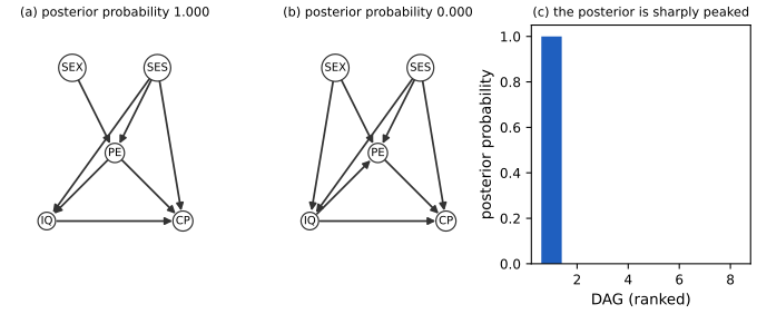
S30.3.3.4 Example: the college plans data. Supplement pp. 240–241 [HMC97] analysed five variables measured for 10 318 Wisconsin high school seniors: sex, socio-economic status (SES), IQ, parental encouragement (PE) and college plans (CP). They computed the exact posterior of all 29 281 five-node DAGs, assigning prior probability 0 to those in which SEX or SES have parents or CP has children, using BDeu with \(\alpha=5\). The most probable graph carries essentially all the mass; it suggests that SES, IQ and PE influence the college decision, that sex acts only through PE, and, surprisingly, a direct link between SES and IQ (perhaps a hidden common cause, revisited in S30.3.8). The data are not distributed with the book. Figure S30.12 redoes the computation on 10 318 cases simulated from the network the supplement later displays (a single hidden binary variable, Figure S30.16, with binary SES and IQ), with the hidden variable discarded: the exact posterior over the allowed DAGs again puts probability 0.9999 on one graph, and that graph has the direct SES-IQ link; the best graph without that adjacency has a log marginal likelihood 59 lower. The simulated data show how a hidden common cause appears as an edge in a model that has no room for it.
S30.3.4 Bayesian model selection: algorithms
Supplement pp. 241–243 Known ordering: K2. If a total order of the nodes is known, the parents of each node can be chosen independently (no cycle is possible): enumerate parent sets among the predecessors and score them. Returning the best set for each node is the K2 algorithm [CH92]; with \(\ell_1\) regularisation the best set is found by a lasso [SNMM07]. Dynamic programming. With an unknown order the globally optimal MAP DAG (up to equivalence) is found by dynamic programming over subsets [KS04; SM06], and posterior edge marginals \(p(G_{st}=1\given\mathcal D)\) likewise [Koi06; PK11], but at cost \(N_G2^{N_G}\), intractable beyond about 16 nodes. For knowledge discovery the MAP DAG can mislead, and edge marginals are the better summary. Size of the space. The number of DAGs on \(D\) nodes obeys Robinson's recurrence (S30.31), with values 1, 3, 25, 543, 29 281, 3 781 503, ... and finding the optimal DAG is NP-complete [Chi96].
Filling the gap 30.9: Robinson's recurrence, and why greedy search and order-based sampling work Supplement pp. 241–243, S(30.31)
Proof
(i) Robinson's recurrence. Let \(a_n\) be the number of labelled DAGs on \(n\) nodes, \(a_0=1\). Every non-empty DAG has at least one source (a node without parents: follow parents backwards; acyclicity ends the walk). Count pairs \((G,S)\) with \(S\) a non-empty set of \(i\) sources of \(G\): choose \(S\) (\(\binom ni\) ways), choose the DAG on the other \(n-i\) nodes (\(a_{n-i}\)), and choose any edges from \(S\) to the rest (\(2^{i(n-i)}\)); no edge may enter \(S\) or join two members of \(S\). Let \(A_S\) be the set of DAGs in which every node of \(S\) is a source. The DAGs we want are the union over singletons \(S=\{v\}\), and by inclusion-exclusion \(\big|\bigcup_vA_{\{v\}}\big|=\sum_{S\ne\emptyset}(-1)^{|S|+1}|A_S|\), since \(\bigcap_{v\in S}A_{\{v\}}=A_S\). Hence \[ a_n=\sum_{i=1}^n(-1)^{i+1}\binom ni2^{i(n-i)}a_{n-i},\qquad a_0=1, \tag{S30.31} \] which gives \(a_1=1\), \(a_2=2\cdot2\cdot1-1=3\), \(a_3=3\cdot4\cdot3-3\cdot2\cdot1+1=25\), \(a_4=543\), \(a_5=29\,281\), \(a_6=3\,781\,503\). (The book writes "for \(D>2\)" with base case \(a_1=1\); the recurrence is valid for all \(n\ge1\) with \(a_0=1\), and the values for \(D=2\) also need \(a_2=3\).) Brute-force enumeration confirms 543 and 29 281.
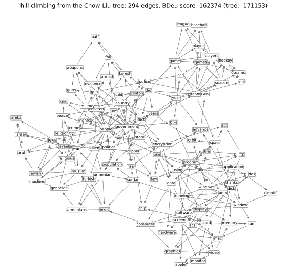
(ii) Greedy hill climbing. By gap 30.8(vi), the neighbours of a DAG under add, delete and reverse moves are scored by at most two family scores each, and only the families of the nodes touched by an accepted move change, so after the first sweep each iteration rescores \(O(D)\) candidates rather than \(O(D^2)\). Acyclicity of an added edge \(s\to t\) is checked by whether \(t\) reaches \(s\) (a transitive closure, \(O(D^3)\), or a search). The search stops at a local maximum; it is initialised at the Chow-Liu tree (gap 30.4) in Figure S30.13. On five nodes the exact global optimum is available by enumeration, and from the empty graph greedy search reaches it on the first 3000 cases of the data of Figure S30.12 (checked: no neighbour is better, and the score equals the global maximum). Searching the space of essential graphs instead (greedy equivalence search, [Chi02]) makes each step more complicated but the space smaller.
(iii) Order-based sampling. Given a total order \(\prec\), \(p(\mathcal D\given\prec)=\prod_t\sum_{\pa\subseteq\{s\prec t\}}\mathrm{score}(t\given\pa)\), because the parent sets are chosen independently and no cycle can arise; the sum is over at most \(2^{t-1}\) sets (or fewer with a fan-in bound). A Metropolis-Hastings chain on orders (swap two neighbours) with this collapsed target mixes faster than a chain on graphs [FK03; EW08]; edge probabilities are averaged over the parent-set posteriors given the order.
S30.3.5 Constraint-based approach
Supplement pp. 243–246 The constraint-based approach learns a DAG up to Markov equivalence (it outputs a PDAG) from local conditional independence tests rather than a global score, and needs no complete model (though each test implicitly assumes one [SP18]). The IC algorithm of Verma and Pearl has three steps: (1) for each pair \(a,b\) look for a set \(S_{ab}\) with \(a\indep b\given S_{ab}\), and connect \(a,b\) in an undirected graph iff none exists; (2) for each non-adjacent pair with a common neighbour \(c\), orient \(a\to c\leftarrow b\) iff \(c\notin S_{ab}\); (3) orient as many remaining edges as possible without creating a new v-structure or a directed cycle, using the three rules of Figure S30.14 (the rules R1–R3 of gap 30.7(iv)). The PC algorithm [SG91] speeds up step 1 by trying separating sets in order of increasing size: start from the complete graph, remove an edge as soon as a separating set is found, first with sets of size 0, then size 1, and so on (Figure S30.15). With the maximal degree \(K\) its cost is \(O(D^{K+1})\) [SGS00].
Filling the gap 30.10: why the PC algorithm returns the essential graph, and the Fisher z test Supplement pp. 243–245
Proof
Assume \(p\) is faithful to a DAG \(G\) and that the independence test is an oracle (it answers by d-separation in \(G\)).
(i) Adjacency. By gap 30.7(i), \(a\) and \(b\) are adjacent in \(G\) iff no set \(S\) makes them conditionally independent. Edges are only deleted when a separating set is found, so no true edge is ever removed.
(ii) The search can be restricted to neighbours. If \(a,b\) are non-adjacent, one of them is not a descendant of the other, say \(b\) of \(a\); then \(a\indep b\given\pa(a)\) (local Markov property), and \(\pa(a)\subseteq\mathrm{adj}(a)\setminus\{b\}\) in the true skeleton. Since the current graph always contains the true skeleton (i), \(\pa(a)\) is a subset of the current neighbours of \(a\) other than \(b\). So if a separating set exists, one exists among the subsets of the neighbours of \(a\) (or of \(b\)) in the current graph, and PC, which tries all subsets of the current neighbours of each end of size \(0,1,2,\dots\) up to the largest neighbourhood, finds one; at the end the graph is exactly the skeleton. Removing edges only shrinks the neighbourhoods, which is why increasing the size level by level is efficient (the stable version used here freezes the neighbourhoods within a level).
(iii) Orientation of v-structures is well defined. For an unshielded triple \(a - c - b\) (\(a,b\) non-adjacent) and any separating set \(S\) of \(a,b\): if \(a\to c\leftarrow b\) is a v-structure, \(c\notin S\) (conditioning on \(c\) or a descendant activates the path); if \(c\) is not a collider on this path, then \(c\in S\) (otherwise the path \(a - c - b\) is active, contradicting separation). So membership of \(c\) in the separating set decides, whichever separating set was found. This is step 2.
(iv) Propagation. Meek's rules (gap 30.7(iv)) orient all remaining edges that every member of the class orients identically. In 300 random six-node DAGs the PC output with a d-separation oracle equalled the essential graph of the truth in every case, and on the five-node graph of Figure S30.15 it removed no edge at size 0, the edges \(A\)-\(C\), \(A\)-\(D\), \(A\)-\(E\), \(C\)-\(D\) at size 1 (each given \(B\)) and \(B\)-\(E\) at size 2 (given \(\{C,D\}\)), as in the figure.
(v) A real test: Fisher's z. For Gaussian data, \(x_a\indep x_b\given\bm x_S\) iff the partial correlation vanishes. If \(\bm P\) is the inverse of the covariance matrix of \((x_a,x_b,\bm x_S)\), the conditional covariance of \((x_a,x_b)\) given \(\bm x_S\) is the inverse of the leading \(2\times2\) block of \(\bm P\) (Schur complement), so the partial correlation is \(\hat\rho_{ab\cdot S}=-P_{ab}/\sqrt{P_{aa}P_{bb}}\). Under the null, \(z=\sqrt{N-|S|-3}\;\mathrm{artanh}\,\hat\rho\) is approximately \(\N(0,1)\); one declares independence when the two-sided \(p\)-value exceeds \(\alpha\). Tests are few at low levels and many at high levels, so errors early in the algorithm (small \(N\)) delete true edges or keep false ones, and the orientation rules then propagate the error: the demonstration shows this, and why one often uses PC to prune the search of a Bayesian method (S30.3.5.3).

S30.3.5.3 Frequentist versus Bayesian. PC relies on an independence oracle. Hypothesis tests (chi-squared for discrete data) work poorly for small samples, face multiple testing, and one wrong test propagates through the constraints. A common hybrid uses PC to build an initial structure and then speeds up Bayesian model selection, which avoids hard independence decisions. One can also learn the undirected skeleton (the Markov blankets) by variable selection instead of tests [PE08].
S30.3.6 Methods based on sparse optimisation
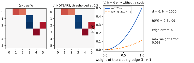
Supplement p. 246 A sparse graph is a sparse adjacency matrix, so one can learn structure by continuous optimisation with a sparsity penalty, as in the lasso (Volume 1, Section 11.4). For undirected graphs this is a convex problem (S30.4.2). For DAGs the acyclicity constraint is the difficulty; [Zhe+18] ("DAGs with no tears", NOTEARS) encode it as a smooth equation, \[ \min_{\bm W\in\R^{D\times D}}f(\bm W)\ \text{s.t.}\ G(\bm W)\in\mathrm{DAGs}\quad\Longleftrightarrow\quad\min_{\bm W}f(\bm W)\ \text{s.t.}\ h(\bm W)=0, \tag{S30.32} \] with the weighted adjacency \(\bm W\), \(G(\bm W)\) the graph of its non-zero entries and the score, for linear Gaussian data, \(f(\bm W)=\frac1{2N}\|\bm X-\bm X\bm W\|_F^2+\lambda\|\bm W\|_1\) (S(30.34)). The constraint function is built from the matrix powers of \(\bm W\): \(h(\bm W)=\Tr\big((\bm I+\alpha\bm W)^D\big)-D\propto\Tr\sum_k\alpha^k\bm W^k\) (S(30.33)), since the diagonal of \(\bm W^k\) counts closed paths of length \(k\). A local optimum of the constrained problem is found by gradient methods at a cost \(O(D^3)\) per iteration. Extensions replace the linear Gaussian model by a VAE with graph neural networks [Yu+19], or by neural network dependencies [Lac+20].
Filling the gap 30.11: what the acyclicity function measures, with a correction Supplement p. 246, S(30.32)–S(30.34)
Proof
(i) Closed walks and cycles. Let \(\bm A\) be a matrix with non-negative entries and \(G(\bm A)\) its graph (edge \(i\to j\) iff \(A_{ij}>0\)). The entry \((\bm A^k)_{ii}=\sum A_{ii_1}A_{i_1i_2}\cdots A_{i_{k-1}i}\) is the total weight of closed walks of length \(k\) through \(i\), a sum of non-negative terms. It is positive iff a closed walk exists, and a closed walk contains a directed cycle, so \(\Tr\bm A^k>0\) for some \(k\) iff \(G(\bm A)\) has a directed cycle. A directed cycle has length at most \(D\), so it suffices to look at \(k\le D\); and if there is no cycle, \(\bm A\) is nilpotent (\(\bm A^D=0\)).
(ii) The constraint functions. Expanding the binomial, \(\Tr(\bm I+\alpha\bm A)^D-D=\sum_{k=1}^D\binom Dk\alpha^k\Tr(\bm A^k)\ge0\), with equality iff all the traces vanish, i.e. iff \(G(\bm A)\) is acyclic. Likewise \(\Tr e^{\bm A}-D=\sum_{k\ge1}\Tr(\bm A^k)/k!\) is zero iff \(G(\bm A)\) is acyclic; this is the form Zheng et al. optimise. The value \(\alpha=1/D\) keeps \((\bm I+\alpha\bm A)^D\) from overflowing.
(iii) The correction: use \(\bm W\circ\bm W\). The argument needs non-negative entries, but \(\bm W\) has weights of both signs. Take \(\bm A=\bm W\circ\bm W\) (elementwise square), which has the same non-zero pattern as \(\bm W\); then \(h(\bm W)=\Tr(\bm I+\alpha\,\bm W\circ\bm W)^D-D\) vanishes iff \(G(\bm W)\) is a DAG. With \(\bm W\) itself, as printed in S(30.33), closed walks of different signs cancel in the trace: for \(D=3\), \(\alpha=1/3\) and \(\bm W=\begin{pmatrix}0&1&0\\-1&0&2\\3&0&0\end{pmatrix}\) (a 2-cycle \(1\leftrightarrow2\) of product \(-1\) and a 3-cycle \(1\to2\to3\to1\) of product 6), \(\Tr\bm W^2=-2\), \(\Tr\bm W^3=18\) and \(h=3\alpha^2\Tr\bm W^2+\alpha^3\Tr\bm W^3=-\tfrac23+\tfrac23=0\), although \(G(\bm W)\) has cycles. The squared form gives \(h>0\) here (confirmed numerically).
(iv) The gradient. For \(h(\bm W)=\Tr e^{\bm W\circ\bm W}-D\), the derivative of the trace of a matrix exponential is \(\partial\Tr e^{\bm A}/\partial\bm A=(e^{\bm A})^{\T}\), and \(\partial A_{ij}/\partial W_{ij}=2W_{ij}\), so \(\nabla h=(e^{\bm W\circ\bm W})^{\T}\circ2\bm W\) (checked by finite differences). The augmented Lagrangian method minimises \(f(\bm W)+\tfrac\rho2h(\bm W)^2+\mu h(\bm W)\) over \(\bm W=\bm W^+-\bm W^-\) with box constraints (so that the \(\ell_1\) penalty is smooth), increasing \(\rho\) tenfold until \(h\) drops by a factor of 4, then \(\mu\leftarrow\mu+\rho h\).
(v) Identifiability. The least squares score is Markov equivalence invariant for general error variances, so the DAG is recovered only up to its class unless the error variances are equal (or the noise non-Gaussian), in which case the DAG is identifiable (Peters and Bühlmann 2014). The experiment of Figure x30.3 uses equal variances. The problem is non-convex: the result is a local optimum.
S30.3.7 Consistent estimators
Supplement pp. 246–247 Can any of these algorithms recover the true DAG, up to equivalence, as \(N\to\infty\), when the data come from a distribution \(p\) faithful to \(G^*\)? Any exact Bayesian procedure is consistent, as are greedy equivalence search [Chi02] and the PC algorithm [SGS00; KB07], though their running time may be exponential, and all assume full observation.
Filling the gap 30.12: consistency of score-based search, in detail Supplement pp. 246–247
Proof
The book says that "the posterior mode converges to the MLE, which converges to the true graph". The MLE of the parameters of a fixed graph does converge, but the statement about the graph needs an argument, which has three steps. Let \(\mathcal M(G)\) be the distributions that factorise on \(G\), so that \(I(G)\subseteq I(p)\) iff \(p\in\mathcal M(G)\) for positive \(p\).
(i) Wrong graphs lose at rate \(N\). For a fixed graph \(G\), by the law of large numbers \(\frac1N\max_{\bm\theta}\log p(\mathcal D\given G,\bm\theta)\to\max_{\bm\theta}\E_p\log p_{\bm\theta}=-\Hent(p)-\min_{\bm\theta}\Dkl(p\|p_{\bm\theta})\) (for a finite model with continuous dependence on \(\bm\theta\) the maximiser converges), and \(\min_{\bm\theta}\Dkl(p\|p_{\bm\theta})=0\) iff \(p\in\mathcal M(G)\). By faithfulness \(I(p)=I(G^*)\), so \(p\in\mathcal M(G)\) iff \(I(G)\subseteq I(G^*)\) (\(G\) is an I-map of \(p\)). A graph that is not an I-map has strictly smaller limiting log-likelihood per case, so it loses by a term of order \(N\); the BIC or Dirichlet marginal likelihood penalty is of order \(\log N\) and cannot compensate.
(ii) Among I-maps the penalty decides. All I-maps reach the same limiting log-likelihood (the entropy of \(p\)), differing by \(O(1)\) terms, so the \(\log N\) penalty on the number of free parameters selects those with the fewest parameters.
(iii) The minimal I-maps are the true class. By a theorem of Chickering (2002), if \(I(G)\subseteq I(G^*)\) then \(G\) has at least as many edges as \(G^*\), with equality iff \(G\equiv G^*\) (I quote this graph-theoretic fact). Since the number of free parameters grows with the edges (for tabular CPDs, \(\sum_tC_t(K_t-1)\)), the unique minimiser of the penalty among I-maps is the equivalence class of \(G^*\) (up to ties among parameter counts, which are broken by equivalence). This is the same conclusion as Haughton (1988) for BIC, and the Dirichlet marginal likelihood has the BIC expansion \(\log p(\mathcal D\given G)=\ell_{\max}-\frac{\dim}{2}\log N+O(1)\), so it is consistent too. The posterior concentrates on the true class.
Numerically: for data simulated from a five-node binary DAG with moderate dependences, the exact posterior over all 29 281 DAGs puts 0.90 of its mass on the true Markov class at \(N=20\,000\) and 0.97 at \(N=100\,000\) (the weakest edges need many cases); PC with Fisher z tests recovers the essential graph for \(N\ge300\) on the demonstration graphs.
S30.3.8 Handling latent variables
Supplement pp. 247–255 If some variables are hidden or missing the complete data assumption fails; the marginal likelihood becomes \[ p(\mathcal D\given G)=\int\sum_{\bm h}p(\mathcal D,\bm h\given\bm\theta,G)\,p(\bm\theta\given G)\d\bm\theta, \tag{S30.35} \] which is intractable (a mixture with \(K\) clusters has \(K^N\) completions, each with a closed-form integral). It also raises new problems: how many hidden variables to add and how to connect them.
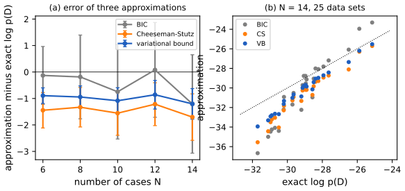
S30.3.8.2–S30.3.8.4 Approximations to the marginal likelihood. BIC: \(\log p(\mathcal D\given\hat{\bm\theta},G)-\tfrac{\log N}2\dim(G)\) (S(30.36)), which can severely underestimate the marginal likelihood [CH97]. Cheeseman-Stutz [CS96]: fit \(\hat{\bm\theta}\) (by EM), fill in the hidden variables by their expected sufficient statistics to get \(\bar{\mathcal D}\), and correct the exact marginal likelihood of the filled-in data, \[ \log p(\mathcal D\given G)\approx\log p(\bar{\mathcal D}\given G)+\log p(\mathcal D\given\hat{\bm\theta},G)-\log p(\bar{\mathcal D}\given\hat{\bm\theta},G). \tag{S30.41} \] Variational Bayes EM: with \(q(\bm\theta,\bm z)=q(\bm\theta)\prod_iq(\bm z_i)\) (S(30.42)); the free energy is a lower bound on the log marginal likelihood and [BG06] found it a much better approximation than BIC or CS.
Filling the gap 30.13: Cheeseman-Stutz, the variational bound against the exact value, and the structural EM inequality Supplement pp. 247–250, S(30.37)–S(30.44)
Proof
(i) Where Cheeseman-Stutz comes from. Write \(\log p(\mathcal D)=\log p(\bar{\mathcal D})+\big[\log p(\mathcal D)-\log p(\bar{\mathcal D})\big]\) (S(30.38)). The first term, with the data completed by expected counts, has a closed-form marginal likelihood (the Dirichlet formula of gap 30.8, valid for fractional counts). The bracket compares two marginal likelihoods of models with the same parameters and prior, so applying the BIC expansion to both, the penalties \(\frac{\log N}2\dim(G)\) cancel and the bracket is approximated by the difference of maximised log-likelihoods \(\log p(\mathcal D\given\hat{\bm\theta})-\log p(\bar{\mathcal D}\given\hat{\bm\theta})\) (S(30.39)–S(30.40)). Adding gives (S30.41). The first term of the bracket is the exact observed-data likelihood at \(\hat{\bm\theta}\) (a sum over hidden states, by inference in the model); the second is the complete-data log-likelihood of the filled-in counts, \(\sum_kN_{k}\log\theta_k\).
(ii) The variational bound is a bound. For any \(q(\bm\theta,\bm z)\), \(\log p(\mathcal D)=\mathcal F(q)+\Dkl\big(q\,\|\,p(\bm\theta,\bm z\given\mathcal D)\big)\ge\mathcal F(q)\) with \(\mathcal F=\E_q\log\frac{p(\mathcal D,\bm z,\bm\theta)}{q(\bm\theta,\bm z)}\). For the latent class model with Dirichlet and Beta priors the VB-EM updates are closed form: \(q(\bm\pi)=\Dir(\alpha+\bar N_k)\), \(q(\theta_{dk})=\mathrm{Beta}(1+\bar N_{dk1},1+\bar N_{dk0})\), with responsibilities \(r_{nk}\propto\exp\big(\E\log\pi_k+\sum_d\E\log\theta_{dk,x_{nd}}\big)\) in terms of digamma functions.
(iii) An experiment against the exact value. For a latent class model (one hidden binary class, three binary features, uniform priors) with \(N\le14\) cases the exact \(\log p(\mathcal D)\) is a sum over \(2^N\) completions. Both CS and VB describe one labelling of the classes, while the exact value integrates over both, so \(\log K!\) must be added to each approximation (for \(K=2\), \(+0.69\)). The exact value agrees with a Monte Carlo estimate over the prior (to two decimals). In 125 simulated data sets (Figure x30.2) the raw VB value is always below the exact value (it is a bound), and after the label correction the average errors (approximation minus exact) are \(-1.00\) for VB, \(-1.45\) for CS and \(-0.44\) for BIC, with standard deviations 0.47, 0.79 and 1.62. So VB is better than CS in bias and spread, as the supplement says; BIC is on average closest here but wildly variable (its error is random, not systematically small), and the claim "VB is always more accurate than CS, which is always more accurate than BIC" is not something one should read as a theorem for such small samples.
(iv) The structural EM inequality. Let \(Q(\bm\theta,G\given\bm\theta_0,G_0)=\E_{\bm h\sim p(\bm h\given\mathcal D,\bm\theta_0,G_0)}\log p(\mathcal D,\bm h\given\bm\theta,G)\). For any \((\bm\theta,G)\), \(\log p(\mathcal D\given\bm\theta,G)=Q(\bm\theta,G\given\bm\theta_0,G_0)+\Hent\big(p(\bm h\given\mathcal D,\bm\theta_0,G_0)\big)+\Dkl\big(p(\bm h\given\mathcal D,\bm\theta_0,G_0)\,\|\,p(\bm h\given\mathcal D,\bm\theta,G)\big)\) (take the expectation of \(\log p(\mathcal D)=\log p(\mathcal D,\bm h)-\log p(\bm h\given\mathcal D)\)). Subtracting the same identity at \((\bm\theta_0,G_0)\), where the KL term is 0, \[ \log p(\mathcal D\given\bm\theta,G)-\log p(\mathcal D\given\bm\theta_0,G_0)\ \ge\ Q(\bm\theta,G\given\bm\theta_0,G_0)-Q(\bm\theta_0,G_0\given\bm\theta_0,G_0). \] The penalties \(\frac{\log N}2\dim(G)\), \(\log p(G)\), \(\log p(\bm\theta\given G)\) are functions of \((\bm\theta,G)\) alone, so they can be added to both sides: a move that improves the penalised expected-data score improves the penalised observed-data score by at least as much. (The direction printed in S(30.44) has the expected-data and observed-data differences interchanged: the guaranteed inequality is the displayed one.) I confirmed it on 200 random pairs of latent class models. Structural EM therefore fills in the data once, with one run of inference in the current model, scores all neighbouring graphs by the expected counts (the complete-data log-likelihood is a sum over families, so this is a decomposable local score again) and moves to the best; it is monotone in the penalised log-likelihood, a generalised EM in the space of graphs.
S30.3.8.5 Example: college plans revisited. Introducing a hidden binary variable \(H\) as a common parent of SES and IQ (and variants with \(H\to\)PE, with the SES-PE and PE-IQ edges dropped or kept, and 2 to 6 states for \(H\): 40 models scored by the CS approximation), [HMC97] found a model with one binary hidden variable (Figure S30.16) that is \(2\cdot10^{10}\) times more likely than the best model without hidden variables and \(5\cdot10^9\) times more likely than the second best with one: again a very peaked posterior. It is read as a hidden "parent quality". The arc \(H\to\)SES can be reversed without changing the v-structures, so hidden variables are hard to interpret; and the model has the same conditional independences among the visible variables as the best visible-only model, so constraint-based methods cannot tell them apart, whereas the Bayesian score, which accounts for parsimony and not just independence, can. The figure itself (a network with conditional probability tables) is not reproduced; its model is the data-generating process of Figure S30.12.
S30.3.8.6 Structural EM. Evaluating every neighbour by running inference is costly because the marginal likelihood (and its approximations) no longer decomposes. The structural EM algorithm [Fri97; Thi+98] fills in the data once using the current model and graph, scores all neighbours on the filled-in data and picks the best, then refits and repeats (refitting only every few steps for speed). It underlies learning of phylogenetic trees, with observed leaves and unobserved internal nodes [Fri+02], and of sparse mixture models, where one decides which features depend on the cluster [BF02] (see also [LFJ04]). The justification is the inequality of gap 30.13(iv).
S30.3.8.7–S30.3.8.10 Discovering hidden variables, Rephil, spectral methods, ADMGs. To find hidden variables one can look for near-cliques in the structure learned over the visible variables (marginalising a hidden parent induces a clique), add a hidden variable and let structural EM sort out the details [Eli+00]; this heuristic works poorly because structure learners are biased against dense cliques. Another idea is clustering: a hidden variable should have high mutual information with its children, and a tree of latent variables, each explaining few children, gives a hierarchical latent class model [Zha04] (finding the optimal latent tree is NP-hard [Roc06]; [HW11] give a fast agglomerative algorithm with two children per latent node, with exact inference in time linear in the nodes, an alternative to topic models). [Cho+11] start from the Chow-Liu tree, add hidden nodes for higher-order dependencies, and can recover the exact latent tree when the data come from one (all variables with the same cardinality). Google's Rephil is a very large learned network: 12 million word nodes, about 1 million latent concept nodes, 350 million noisy-OR links, depth 555, trained on about \(10^{11}\) snippets and used in advertising; structure is learned by "fire together, wire together", merging, pruning, and inference by iterated conditional modes in milliseconds. These models are described but not reproduced (figures S30.17–S30.20). Spectral methods give identifiability, with the method of moments, for three or more independent views of the latent variable, for a latent categorical variable with Gaussian mixture children [Ana+14], and for binary latents with noisy-OR children [JHS13; Aro+16]. Finally one can marginalise the latent variables and work with acyclic directed mixed graphs, with Bayesian selection [SG09] or the IC*/FCI algorithms [Pea09; SGS00] whose output is a partially oriented inducing path graph with four kinds of edge mark (marked arrow, unmarked arrow, bidirected, undirected); FCI shares the weaknesses of PC and the output cannot be used for prediction.
S30.4 Learning undirected graph structures supplement
Supplement pp. 255–261 Learning undirected structure is easier than learning a DAG in one respect (no acyclicity constraint) and harder in another: the likelihood does not decompose over the graph because of the global partition function (Section 4.3.9). Greedy search and MCMC are then too expensive, since scoring a neighbour needs a refit from scratch. The solutions below avoid or approximate the partition function.
S30.4.1 Dependency networks
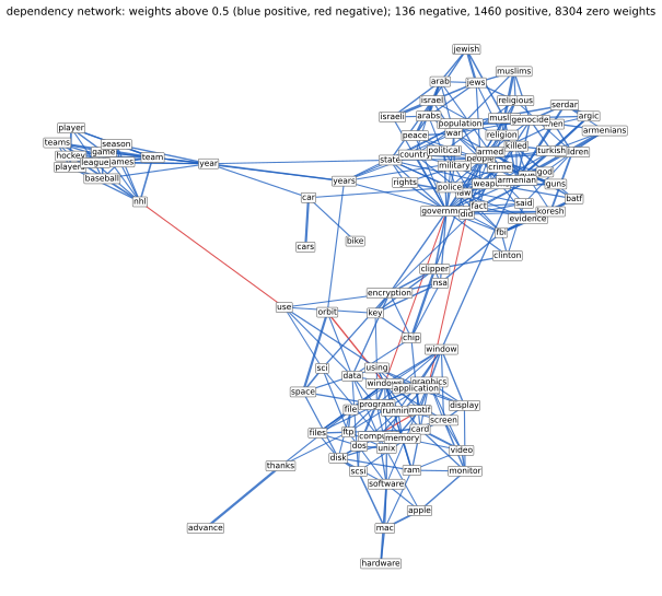
Supplement pp. 255–257 A simple way to learn the structure of an undirected model is to learn each full conditional \(p(x_d\given\bm x_{-d})\) separately and define \[ p(\bm x)\;\propto\;\prod_{d=1}^Dp(x_d\given\bm x_{-d}) \tag{S30.45} \] (the pseudo-likelihood). A product of independently estimated full conditionals need not be consistent with any joint distribution, but the collection (a dependency network [Hec+00]) can still be used in a Gibbs sampler, for example for imputation. The main advantage is that each conditional can be estimated by a sparse regression, whose non-zero coefficients are the Markov blanket: classification trees [Hec+00], \(\ell_1\)-regularised linear regression [MB06] or logistic regression [WRL06; WSD19], Bayesian variable selection [Dob09]. Figure S30.21 shows a dependency network for the newsgroups data, with each penalty chosen by BIC; the weights are informative, since negative ones (dissociation) are as meaningful as positive ones.
S30.4.2 Graphical lasso for GGMs
Supplement pp. 257–258 For a Gaussian graphical model there is a one-to-one map between sparse parameters and sparse structures: \(\Omega_{st}=0\) iff there is no edge \(s-t\). This lets us use \(\ell_1\) estimation (Volume 1, Section 11.4); the method is the graphical lasso or glasso [FHT08; MH12].
S30.4.2.1 MLE for a GGM. Computing the MLE of a non-decomposable GGM is covariance selection [Dem72]. With \(\hat{\bm\mu}=\bar{\bm x}\) and the empirical covariance \(\bm S\), the log-likelihood per case, up to a constant, is \[ \ell(\bm\Omega)=\log\det\bm\Omega-\Tr(\bm S\bm\Omega), \tag{S30.46} \] with gradient \(\nabla\ell(\bm\Omega)=\bm\Omega^{-1}-\bm S\) (S(30.47)); one must enforce \(\Omega_{st}=0\) for absent edges, easy, and positive definiteness, a convex but non-trivial constraint (handled by a penalty [DVR08] or by coordinate descent [HTF09, p. 633]). The MLE satisfies \(\Sigma_{st}=S_{st}\) whenever \(G_{st}=1\) or \(s=t\), and \(\Omega_{st}=0\) otherwise: \(\bm\Sigma\) is a positive definite matrix completion of \(\bm S\), keeping the entries of \(\bm S\) on the edges and filling the rest to maximise the likelihood. Worked example (from [HTF09, p. 652]): for the cycle \(X_1-X_2-X_3-X_4-X_1\) and \[ \bm S=\begin{pmatrix}10&1&5&4\\1&10&2&6\\5&2&10&3\\4&6&3&10\end{pmatrix}\ \text{the MLE is}\ \hat{\bm\Sigma}=\begin{pmatrix}10.00&1.00&1.31&4.00\\1.00&10.00&2.00&0.87\\1.31&2.00&10.00&3.00\\4.00&0.87&3.00&10.00\end{pmatrix},\ \hat{\bm\Omega}=\begin{pmatrix}0.12&-0.01&0&-0.05\\-0.01&0.10&-0.02&0\\0&-0.02&0.11&-0.03\\-0.05&0&-0.03&0.13\end{pmatrix}. \tag{S30.49} \] (The book prints 0.11 for \(\hat\Omega_{22}\); it is 0.105.) The entries of \(\bm\Sigma\) that were free to change are \(\Sigma_{13}\) and \(\Sigma_{24}\), the absent edges.
S30.4.2.2 Promoting sparsity. The \(\ell_1\)-penalised negative log-likelihood is \[ J(\bm\Omega)=-\log\det\bm\Omega+\Tr(\bm S\bm\Omega)+\lambda\|\bm\Omega\|_1,\qquad\|\bm\Omega\|_1=\sum_{j,k}|\omega_{jk}|. \tag{S30.50} \] It is convex, non-smooth and constrained to \(\bm\Omega\succ0\). Algorithms exist [YL07; BGd08; DGK08]; the simplest is block coordinate descent of [FHT08], and an even faster method uses soft thresholding [FS18; FZS18]. Figure 30.1 (Section 30.3.2) shows the graphs learned on the flow cytometry data as \(\lambda\) is swept; the data were sampled under intervention, which this method ignores, and the learned graphs can contain the feedback loops that a DAG cannot (compare the DAG of Main Figure 20.7, and the discussion in [SM09]). The graphical lasso is not model-selection consistent [Mei05].
Filling the gap 30.15: the Gaussian MLE, the optimality conditions and the graphical lasso algorithm Supplement pp. 257–258, S(30.46)–S(30.50)
Proof
(i) The log-likelihood and its gradient. For \(N\) cases from \(\N(\bm\mu,\bm\Omega^{-1})\), \(\sum_i\log p(\bm x_i)=\frac N2\big[\log\det\bm\Omega-\Tr(\bm S\bm\Omega)\big]-\frac{ND}2\log2\pi\) at \(\bm\mu=\bar{\bm x}\), since \(\sum_i(\bm x_i-\bar{\bm x})^{\T}\bm\Omega(\bm x_i-\bar{\bm x})=N\Tr(\bm S\bm\Omega)\). By Jacobi's formula \(\d\log\det\bm\Omega=\Tr(\bm\Omega^{-1}\d\bm\Omega)\) and \(\d\Tr(\bm S\bm\Omega)=\Tr(\bm S\,\d\bm\Omega)\), so the derivative in direction \(\d\bm\Omega\) is \(\Tr\big((\bm\Omega^{-1}-\bm S)\d\bm\Omega\big)\): this is S(30.47) (a finite difference check agrees). \(\log\det\) is strictly concave on the positive definite cone and \(\Tr(\bm S\bm\Omega)\) is linear, so \(\ell\) is strictly concave (when \(\bm S\succ0\)).
(ii) The constrained MLE. Maximise \(\ell\) over the subspace of matrices with \(\Omega_{st}=0\) for non-edges. Parametrise it by the free entries (the diagonal and the edges); the gradient with respect to a free entry \(\Omega_{st}\) is \((\bm\Omega^{-1}-\bm S)_{st}\) (times 2 off the diagonal), which must vanish at an interior maximum. Hence \(\Sigma_{st}=S_{st}\) on the diagonal and the edges, while \(\Omega_{st}=0\) off them: the two properties of the text, and by strict concavity the solution is unique when it exists (it exists iff \(\bm S\) has a positive definite completion on the pattern). Algorithm (modified regression). Let \(\bm W\) be the current estimate of \(\bm\Sigma\) and partition it with node \(j\) last: \(\bm W=\begin{pmatrix}\bm W_{11}&\bm w_{12}\\\bm w_{12}^{\T}&w_{22}\end{pmatrix}\). From \(\bm W\bm\Omega=\bm I\) one gets \(\bm w_{12}=\bm W_{11}\bm\beta\) with \(\bm\beta=-\bm\omega_{12}/\omega_{22}\), so the last column of \(\bm\Omega\) is zero outside the neighbours of \(j\) iff \(\bm\beta\) is. The condition \(\bm w_{12}=\bm s_{12}\) on the neighbour entries then reads \(\bm W_{11}[N,N]\bm\beta_N=\bm s_{12}[N]\), where \(N\) is the neighbour set. Cycling over \(j\), solving this small system and updating \(\bm w_{12}=\bm W_{11}\bm\beta\) (padding \(\bm\beta\) with zeros), converges to the fixed point that satisfies both conditions. On the example above this reproduces S(30.49): \(\Sigma_{13}=1.31\), \(\Sigma_{24}=0.87\), and the zeros of \(\bm\Omega\) are exact.
(iii) Optimality conditions of the graphical lasso. \(J\) is convex. At a minimiser \(\bm\Omega\succ0\), \(0\in\partial J\): \(-\bm\Omega^{-1}+\bm S+\lambda\bm\Gamma=0\) with \(\Gamma_{jk}=\sgn(\Omega_{jk})\) where \(\Omega_{jk}\ne0\) and \(\Gamma_{jk}\in[-1,1]\) where \(\Omega_{jk}=0\). With \(\bm W=\bm\Omega^{-1}\): \[ W_{jj}=S_{jj}+\lambda,\qquad W_{jk}-S_{jk}=\lambda\sgn(\Omega_{jk})\ \text{if}\ \Omega_{jk}\ne0,\qquad |W_{jk}-S_{jk}|\le\lambda\ \text{if}\ \Omega_{jk}=0 \] (for the diagonal \(\Omega_{jj}>0\) and the diagonal is penalised, as in S(30.50); if only the off-diagonal were penalised, \(W_{jj}=S_{jj}\)). No edges iff \(\lambda\ge\max_{j\ne k}|S_{jk}|\): the diagonal matrix \(\bm\Omega=(\diag\bm S+\lambda\bm I)^{-1}\), with \(\bm W=\diag\bm S+\lambda\bm I\), satisfies all the conditions when \(\lambda\ge\max|S_{jk}|\) (its diagonal is \(S_{jj}+\lambda\), and the off-diagonal \(W_{jk}-S_{jk}=-S_{jk}\) lies in \([-\lambda,\lambda]\)), so by uniqueness (strict convexity) it is the solution; if some \(|S_{jk}|>\lambda\) it violates the condition, so an edge appears. On the flow cytometry data this occurs for \(\lambda\ge\max|S_{jk}|\) and an edge appears just below (confirmed).
(iv) Block coordinate descent. Partition as in (ii) with \(\bm\Omega=\begin{pmatrix}\bm\Theta_{11}&\bm\theta_{12}\\\bm\theta_{12}^{\T}&\theta_{22}\end{pmatrix}\). The identity \(\bm W\bm\Omega=\bm I\) gives \(\bm w_{12}=-\bm W_{11}\bm\theta_{12}/\theta_{22}=\bm W_{11}\bm\beta\) with \(\bm\beta=-\bm\theta_{12}/\theta_{22}\); since \(\theta_{22}>0\), \(\sgn(\bm\theta_{12})=-\sgn(\bm\beta)\). The off-diagonal block of the optimality condition becomes \(\bm W_{11}\bm\beta-\bm s_{12}+\lambda\,\sgn(\bm\beta)\ni0\) (with \(\bm W_{11}\) held fixed, as block coordinate descent does). This is exactly the optimality condition of the lasso problem \(\min_{\bm\beta}\tfrac12\bm\beta^{\T}\bm W_{11}\bm\beta-\bm s_{12}^{\T}\bm\beta+\lambda\|\bm\beta\|_1\), i.e. the lasso regression of node \(j\) on the others with the Gram matrix \(\bm W_{11}\) of the current covariance estimate and the cross-product vector \(\bm s_{12}\). It is solved by coordinate descent: \(\beta_k\leftarrow\mathrm{soft}\big(s_{k}-\sum_{l\ne k}W_{kl}\beta_l,\lambda\big)/W_{kk}\), \(\mathrm{soft}(u,\tau)=\sgn(u)\max(|u|-\tau,0)\). After convergence \(\bm w_{12}\leftarrow\bm W_{11}\bm\beta\); cycling over \(j\) until \(\bm W\) stops changing gives the solution, and \(\bm\Omega\) is recovered by the block inverse, \(\theta_{22}=1/(w_{22}-\bm w_{12}^{\T}\bm\beta)\), \(\bm\theta_{12}=-\bm\beta\theta_{22}\). My implementation agrees with scikit-learn's graphical lasso (which penalises only the off-diagonal) to \(10^{-11}\) when the diagonal is left unpenalised, satisfies the conditions above on the flow cytometry data at \(\lambda=7\), and its objective is below the objective at 100 random feasible perturbations.
(v) The sample-size effect. The estimate depends on the data only through \(\bm S\); with few cases \(\bm S\) is noisy and false edges survive, which the demonstration shows (60 versus 1000 cases of a chain).
S30.4.3 Graphical lasso for discrete MRFs and CRFs
Supplement p. 259 For discrete models every edge has a block of parameters, so the lasso becomes a group lasso (Volume 1, Section 11.4.7). For a pairwise CRF with node and edge potentials linear in \(\bm x\) (S(30.51)) one minimises \[ J=-\sum_i\Big[\sum_t\log\psi_t(y_{it},\bm x_i,\bm v_t)+\sum_{s<t}\log\psi_{st}(y_{is},y_{it},\bm x_i,\bm w_{st})\Big]+\lambda_1\sum_{s<t}\|\bm w_{st}\|_p+\lambda_2\sum_t\|\bm v_t\|_2^2, \tag{S30.52} \] with \(p=2\) or \(\infty\) ([Sch+08]; for binary MRFs [LGK06]). It is convex but each evaluation needs inference (the global partition function): use few evaluations (a projected quasi-Newton method [Sch+09]) or loopy belief propagation. A much faster alternative applies the group lasso to the pseudo-likelihood, with no inference [HT09] (Figure S30.22). The GRISE estimator [VML19] of sparse full conditionals takes polynomial time with near-optimal sample complexity [Lok+18].
Filling the gap 30.14: nodewise regression, incompatible conditionals, the pseudo-likelihood for binary MRFs, and the group lasso step Supplement pp. 255–259, S(30.45), S(30.52)
Proof
(i) Neighbours are the support of a regression. For \(\bm x\sim\N(\bm 0,\bm\Omega^{-1})\) the full conditional of \(x_d\) has density \(\propto\exp\big(-\tfrac12\Omega_{dd}x_d^2-x_d\sum_{j\ne d}\Omega_{dj}x_j\big)\) (the terms of \(\tfrac12\bm x^{\T}\bm\Omega\bm x\) containing \(x_d\)); completing the square gives \(x_d\given\bm x_{-d}\sim\N\big(-\sum_{j\ne d}\tfrac{\Omega_{dj}}{\Omega_{dd}}x_j,\ \tfrac1{\Omega_{dd}}\big)\). The population regression coefficients are therefore \(-\Omega_{dj}/\Omega_{dd}\), zero iff \(\Omega_{dj}=0\) iff there is no edge: the Markov blanket of \(d\) is the support of the regression. The lasso estimates this support, node by node [MB06], and the graph combines the \(D\) supports by "and" or "or" (an edge needs both nodes to select each other, or at least one). Their theory requires the irrepresentable condition. (Checked numerically: for a precision matrix with off-diagonals 0.3 the population coefficients equal \(-\Omega_{dj}/\Omega_{dd}\).)
(ii) Independent conditionals can be incompatible. Two binary variables, with conditionals \(a_u=p(x_1=1\given x_2=u)\) and \(b_v=p(x_2=1\given x_1=v)\) estimated separately. For any positive joint \(p\), the odds ratio is symmetric: \(\frac{a_1/(1-a_1)}{a_0/(1-a_0)}=\frac{p_{11}p_{00}}{p_{01}p_{10}}=\frac{b_1/(1-b_1)}{b_0/(1-b_0)}\). So the tables are compatible with a joint only if the two odds ratios agree (and then a joint exists: choose \(p_{00}\) and solve). With \(a=(0.5,0.9)\) (odds ratio 9) and \(b=(0.5,0.6)\) (odds ratio 1.5) no joint has these conditionals; the product (S30.45) is then not a normalised distribution with those conditionals as its own, and Gibbs sampling from it (a "pseudo-Gibbs sampler") has a stationary law that depends on the order of the sweeps.
(iii) The pseudo-likelihood of a binary pairwise MRF. For \(x_t\in\{-1,+1\}\) and \(p(\bm x)\propto\exp\big(\sum_tb_tx_t+\sum_{s<t}w_{st}x_sx_t\big)\), the log odds of \(x_t=+1\) against \(-1\) given the rest are \(2\big(b_t+\sum_{s\ne t}w_{ts}x_s\big)\) (the terms not containing \(x_t\) cancel, including the partition function), so \(p(x_t\given\bm x_{-t})=\sigma\big(2x_t(b_t+\sum_sw_{ts}x_s)\big)\). The negative log pseudo-likelihood is \(-\frac1N\sum_n\sum_t\log\sigma(2x_{nt}h_{nt})\), \(h_{nt}=b_t+\sum_sw_{ts}x_{ns}\), convex in \((\bm b,\bm W)\), and with the penalty \(\lambda\sum_{s<t}|w_{st}|\) (one coupling per edge, shared by the two conditionals) it is minimised by a proximal gradient method: a gradient step on the smooth part, then soft thresholding of each \(w_{st}\) at \(\lambda/L\); the gradient is \(-2x\,\sigma(-2xh)\) in \(h\) (accelerated: FISTA). The step is \(1/L\) with \(L\) bounding the largest curvature (the second derivative of \(-\log\sigma(2u)\) is at most 1). Figure S30.22 uses \(\lambda=0.08\).
(iv) The group lasso step. For edges with parameter blocks \(\bm w_{st}\) the penalty is \(\lambda\|\bm w_{st}\|_2\) and its proximal map solves \(\min_{\bm u}\tfrac12\|\bm u-\bm v\|^2+\tau\|\bm u\|\). If \(\|\bm v\|\le\tau\) the minimiser is \(\bm u=\bm0\) (the subdifferential of the norm at 0 is the unit ball, which contains \(\bm v/\tau\)). Otherwise the minimiser is non-zero and \(\bm u-\bm v+\tau\bm u/\|\bm u\|=0\), so \(\bm u\) is parallel to \(\bm v\) with \(\|\bm u\|=\|\bm v\|-\tau\): \(\bm u=\max(0,1-\tau/\|\bm v\|)\,\bm v\) (block soft thresholding). A whole block of parameters is zero together, so an edge is either present with all its parameters or absent; for binary variables the block has one entry and the group lasso is the ordinary lasso. With \(p=\infty\) the dual ball is the \(\ell_1\) ball, with a more involved projection.
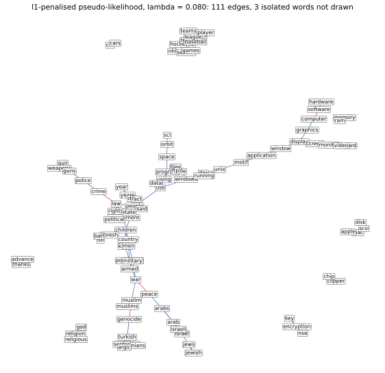
S30.4.4 Bayesian inference for undirected graph structures
Supplement pp. 259–261 The graphical lasso gives only a point estimate and is not model-selection consistent. A Bayesian treatment integrates out the parameters and computes \(p(G\given\mathcal D)\) and edge marginals \(p(G_{ij}=1\given\mathcal D)\). For decomposable (chordal) graphs with conjugate priors the marginal likelihood is available in closed form [DL93] and the decomposable neighbours of a graph are cheap to enumerate [TG09b], so stochastic local search is feasible [GG99; Arm+08; SC08]. But decomposable graphs are a vanishing fraction of all graphs: the numbers of decomposable graphs on \(2,\dots,8\) nodes are 2, 8, 61, 822, 18 154, 617 675, 30 888 596 against \(2^{N_G(N_G-1)/2}\) undirected graphs, ratios 1, 1, 0.95, 0.80, 0.55, 0.29, 0.12. (I verified the first five counts by enumerating all graphs and testing chordality; the book prints the sixth as "61,7675".) For non-decomposable Gaussian graphs one needs approximations to the marginal likelihood under a G-Wishart prior [Rov02]: Monte Carlo is slow [AKM05], a Laplace approximation needs the MAP estimate, found by iterative proportional scaling [LD08] (which needs the cliques, NP-hard in general) or, much faster, by the gradient methods of S30.4.2.1 [Mog+09], with a diagonal Laplace approximation that is more accurate than BIC at the same cost; this outperformed the graphical lasso in prediction and structure recovery.
30.3.2 Applications
pp. 1044–1045 There are three main reasons to learn the structure of a probabilistic graphical model: understanding, prediction and causal inference.
Understanding. Sparse graphs help to understand how many variables interact. In systems biology, [Sac+05] measured the phosphorylation status of proteins in a cell by flow cytometry (7466 cells, 11 proteins); the graphical lasso yields the graphs of Figure 30.1 as the sparsity level \(\lambda\) changes. Other examples: the neural "wiring diagram" of a bird recovered from multivariate EEG time series [Smi+06].
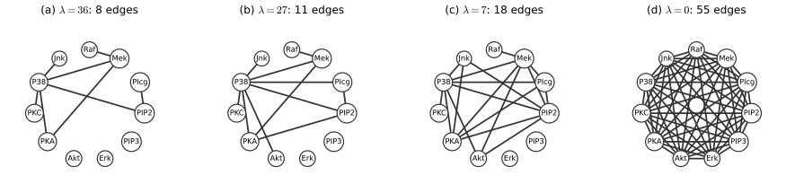
Prediction. Sometimes the graph is used only to predict. In portfolio management a sparse graph of the covariance of many stocks can be the basis of a trading strategy that beats methods without sparsity [CW07]; the deployed JamBayes system predicts traffic jams near Seattle with a directed model whose structure was learned from data [Hor+05].
Causal inference. To predict the effect of interventions, or to reason about counterfactuals, we need a structural causal model (Section 4.7): a directed model whose non-root relations are deterministic. Techniques for learning DAGs can therefore learn structural causal models if we assume something about confounders; this is causal discovery (Section S30.5).
S30.5 Learning causal DAGs supplement
Supplement pp. 261–266 Causal reasoning depends on knowing the DAG (though [JZB19] answer some queries knowing it only up to Markov equivalence); learning it is causal discovery [GZS19]. With two variables the models \(X\to Y\) and \(X\leftarrow Y\) are Markov equivalent, so they cannot be told apart from observational data, yet they make different causal predictions (S30.5.1). With more variables we need general methods, and interventions to shrink the equivalence class [Sol19] (S30.5.2). When the data are low level (pixels) the causal variables must be learned (S30.5.3). Further reading: [Ebe17; PJS17; HDMM18; Guo+21].
S30.5.1 Learning cause-effect pairs
Supplement pp. 261–265 Conditional independence tests need three variables, but intuitively causal relations of pairs can be learned: altitude causes temperature, not conversely. Measure both in two countries, the Netherlands (low) and Switzerland (high): in the factorisation \(p(X)p(Y\given X)\) the mechanism \(p(Y\given X)\) is stable across the populations and only \(p(X)\) changes, while in \(p(Y)p(X\given Y)\) both factors must change; the causal factorisation is the "simpler" one. The following methods exploit this idea, following [PJS17].
S30.5.1.1 Algorithmic information theory. With \(X\in\{0,1\}\) and \(Y\in\R\), \[ p(x,y)=\Ber(x\given\theta)\,\N(y\given\mu_x,1)\ \Longleftrightarrow\ p(y)\,p(x\given y)=\big[\theta\N(y\given\mu_1,1)+(1-\theta)\N(y\given\mu_0,1)\big]\,\Ber\big(x\given\sigma(\alpha+\beta y)\big) \tag{S30.53--S30.54} \] (my notation: \(\mu_1,\mu_0\) are the means when \(x=1,0\); the supplement calls them \(\mu_1,\mu_2\)), with \(\alpha=\mathrm{logit}(\theta)+(\mu_0^2-\mu_1^2)/2\) and \(\beta=\mu_1-\mu_0\). The first form (\(X\to Y\)) consists of two simple generic distributions; in the second, \(p(Y)\) is a more complex mixture tied to the specific form of \(p(X\given Y)\). [JS10] formalise this: \(X\) causes \(Y\) if \(P_X\) and \(P_{Y\given X}\) are algorithmically independent, \(K(P_{X,Y})=K(P_X)+K(P_{Y\given X})\) with \(K\) the Kolmogorov complexity (S(30.55)). Since \(K\) cannot be computed this is only conceptual.
S30.5.1.2 Additive noise models. A general SCM \(X\to Y\) with \(Y=f_Y(X,U_Y)\) is not identifiable from finite data: if \(U\) merely selects a function \(f_u\) the induced law is a mixture of mappings. For instance with \(X\) and \(U\) Bernoulli and \(U\) choosing between identity and negation, \(Y\) is uniform and independent of \(X\) even though \(X\to Y\). One restricts the functions: additive noise models (ANM) [Hoy+09], \(X_i=f_i(X_{\pa(i)})+U_i\) (S(30.56)); for two variables \(Y=f(X)+U\). If \(X,U\) are Gaussian and \(f\) linear the law is jointly Gaussian and symmetric, so the direction is not identified; with a nonlinear \(f\), or a non-Gaussian \(X\) or \(U\), it is.
S30.5.1.3 Nonlinear additive noise models. For \(Y=f(X)+U\) with \(f\) nonlinear, in general there is no ANM in the other direction. So regress \(Y\) on \(X\) nonlinearly and test whether the residual is independent of \(X\); then swap the roles. The theory [PJS17] says the test passes only in the causal direction (Figure S30.23).
S30.5.1.4 Linear models with non-Gaussian noise. With a linear \(f\) and Gaussian noise the symmetry of Figure S30.23 remains; with non-Gaussian noise identifiability returns. ICA (Section 28.6) is the noise-free case, \(\bm y=\bm A\bm x\) with non-Gaussian sources; intuitively linear combinations tend to be more Gaussian (central limit theorem), so if \(X\to Y\) then \(p(Y)\) looks more Gaussian than \(p(X)\). With non-Gaussian observation noise, \(\bm y=\bm A\bm x+\bm U_Y\), we have a "linear non-Gaussian acyclic model" (LiNGAM) [Shi+06], whose joint law differs between \(X\to Y\) and \(Y\to X\).
Filling the gap 30.16: the logistic form, the Gaussian symmetry, and identifiability of linear non-Gaussian models Supplement pp. 262–263, S(30.53)–S(30.56)
Proof
(i) S(30.54). By Bayes' rule, \(p(x=1\given y)=\dfrac{\theta\N(y\given\mu_1,1)}{\theta\N(y\given\mu_1,1)+(1-\theta)\N(y\given\mu_0,1)}=\sigma\Big(\log\tfrac{\theta}{1-\theta}+\log\tfrac{\N(y\given\mu_1,1)}{\N(y\given\mu_0,1)}\Big)\), and \(\log\frac{\N(y\given\mu_1,1)}{\N(y\given\mu_0,1)}=-\tfrac12(y-\mu_1)^2+\tfrac12(y-\mu_0)^2=(\mu_1-\mu_0)y+\tfrac12(\mu_0^2-\mu_1^2)\). Hence \(\alpha=\mathrm{logit}\,\theta+\frac12(\mu_0^2-\mu_1^2)\) and \(\beta=\mu_1-\mu_0\); the supplement's text is missing the factor \(\tfrac12\) in \(\alpha\) (confirmed numerically on a grid of \(y\)).
(ii) The Gaussian case is symmetric. If \((X,Y)\) is jointly Gaussian with variances \(\sigma_x^2,\sigma_y^2\) and correlation \(\rho\), then \(Y=aX+U\) with \(a=\rho\sigma_y/\sigma_x\) and \(U=Y-aX\), which is Gaussian and uncorrelated with, hence independent of, \(X\); and in the same way \(X=bY+V\) with \(b=\rho\sigma_x/\sigma_y\), \(V\) independent of \(Y\). Both directions are valid linear ANMs.
(iii) The unidentifiable example. \(X,U\sim\Ber(\tfrac12)\) independent and \(Y=\Ind[X=U]\): \(\Pr(Y=1\given X=x)=\Pr(U=x)=\tfrac12\) for both \(x\), so \(X\indep Y\) although \(X\) is a parent; the graph is unfaithful and the structure invisible.
(iv) Linear non-Gaussian models are identified. I use the Darmois-Skitovich theorem (quoted): if \(L_1=\sum a_iZ_i\) and \(L_2=\sum b_iZ_i\) are linear forms in independent random variables \(Z_i\) and \(L_1\indep L_2\), then every \(Z_i\) with \(a_ib_i\ne0\) is Gaussian. Suppose \(Y=aX+U\) with \(X\indep U\), \(a\ne0\), and that there is also a backward model \(X=bY+V\) with \(V\indep Y\). Then \(b\ne0\) (else \(X\indep Y\), contradicting \(\cov(X,Y)=a\var X\ne0\)) and \[ V=X-bY=(1-ab)X-bU,\qquad Y=aX+U. \] These are linear forms in \(X,U\); \(U\) has coefficients \(-b\ne0\) and 1, so by the theorem \(U\) is Gaussian; \(X\) has coefficients \(1-ab\) and \(a\ne0\), so \(X\) is Gaussian unless \(ab=1\). If \(ab=1\), then \(V=-bU\) and \(V\indep Y=aX+U\) gives \(\cov(U,aX+U)=\var U=0\), so \(U\) is constant. Conclusion: if \(U\) is non-Gaussian (and non-degenerate), the data admit an ANM in at most one direction; the direction is identified. If \(X\) and \(U\) are both Gaussian, both directions work ((ii)).
(v) Nonlinear ANM. The result for nonlinear \(f\) [Hoy+09; PJS17] is quoted: if both directions admit an ANM, \(f\), \(p_X\) and \(p_U\) satisfy a differential equation that holds only in exceptional cases (for example linear \(f\) with Gaussian variables, or special exponentials). I confirm it by simulation rather than prove it.
(vi) Testing independence. The residual \(r\) and the regressor \(x\) are compared by the Hilbert-Schmidt independence criterion, \(\mathrm{HSIC}=\|\mathcal C_{xr}\|_{HS}^2\), which is 0 iff \(x\indep r\) for characteristic (Gaussian) kernels [Gre+05]; the biased estimate is \(\Tr(\bm K\bm H\bm L\bm H)/N^2\) with Gram matrices \(\bm K,\bm L\) (kernel widths: median distances) and \(\bm H=\bm I-\bm 1\bm 1^{\T}/N\); a permutation test gives \(p\)-values. With cases \(N=500\) of the three demonstration data sets: for the nonlinear model with Gaussian noise (a degree 5 polynomial fit) the HSIC is 0.00036 in the causal direction (permutation \(p=0.43\), 200 permutations) against 0.0042 (\(p=0.005\)); for the linear Gaussian model neither direction is rejected (\(p=0.48\) and \(0.22\)); for linear uniform noise the wrong direction is rejected (HSIC 0.0045, \(p=0.005\)) and the right one is not (0.0003, \(p=0.53\)). A linear fit to the nonlinear data, or a polynomial that cannot represent \(f\), gives dependent residuals in both directions and the test is uninformative: the regression must be flexible enough.
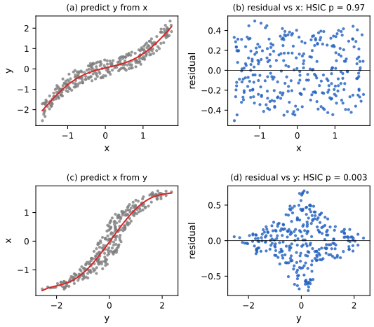
S30.5.1.5 Information-geometric causal inference. The IGCI method [Dan+10; Jan+12] assumes a deterministic, strictly increasing \(f\) on \([0,1]\) with \(f(0)=0\), \(f(1)=1\), and \(Y=f(X)\). The peaks of \(p_Y\) occur where \(f\) is flat (\(f^{-1}\) steep), so \(p_Y\) and \(f^{-1}\) are related, while \(p_X\) and \(f\) are not (Figure S30.24). View \(\log f'\) and \(p_X\) as random variables on \([0,1]\) with the uniform measure; the model satisfies IGCI if \(\mathrm{Cov}[\log f',p_X]=\int_0^1\log f'(x)p_X(x)\d x-\int_0^1\log f'(x)\d x=0\) (S(30.57)), and then \(\mathrm{Cov}[\log(f^{-1})',p_Y]\ge0\) with equality iff \(f\) is linear. The slope-based test is \[ \hat C_{X\to Y}=\frac1{N-1}\sum_{j=1}^{N-1}\log\frac{|y_{j+1}-y_j|}{|x_{j+1}-x_j|}\approx\int_0^1\log f'(x)p(x)\d x,\tag{S30.58} \] with the \(x_j\) sorted, and \(\hat C_{Y\to X}\) analogous; choose \(X\to Y\) if \(\hat C_{X\to Y}<\hat C_{Y\to X}\). An IGCI model also has \(H(X)\le H(Y)\) according to the supplement (it says that applying \(f\) adds irregularity so \(p_Y\) is less uniform), and one can choose the direction by entropy estimates [Moo+16].
Filling the gap 30.17: the IGCI identities, and a sign error in the entropy statement Supplement pp. 264–265, S(30.57)–S(30.58)
Proof
Let \(f:[0,1]\to[0,1]\) be a strictly increasing, differentiable bijection (\(f'>0\)), \(X\sim p_X\), \(Y=f(X)\), so \(p_Y(f(x))f'(x)=p_X(x)\).
(i) \(C_{Y\to X}=-C_{X\to Y}\). Define \(C_{X\to Y}=\int\log f'(x)p_X(x)\d x\) and \(C_{Y\to X}=\int\log(f^{-1})'(y)p_Y(y)\d y\). With \(y=f(x)\), \((f^{-1})'(f(x))=1/f'(x)\) and \(p_Y(y)\d y=p_X(x)\d x\), so \(C_{Y\to X}=-\int\log f'(x)p_X(x)\d x=-C_{X\to Y}\). Hence the rule "\(\hat C_{X\to Y}<\hat C_{Y\to X}\)" is the rule "\(\hat C_{X\to Y}<0\)". The same holds exactly for the estimators: for increasing \(f\) the sorted-by-\(x\) and sorted-by-\(y\) sample points coincide, so \(\hat C_{Y\to X}=-\hat C_{X\to Y}\) (confirmed).
(ii) Under IGCI, \(C_{X\to Y}\le0\). IGCI says \(\int\log f'(x)p_X(x)\d x=\int\log f'(x)\d x\) (S(30.57); the second integral is over \([0,1]\) with \(\int p_X=1\)). By Jensen, \(\int_0^1\log f'\d x\le\log\int_0^1f'\d x=\log(f(1)-f(0))=0\), with equality iff \(f'\equiv1\). So \(C_{X\to Y}\le0\le C_{Y\to X}\) and the rule is right in the population (strictly unless \(f\) is the identity).
(iii) The claim about \(f^{-1}\). By (i)-(ii) and the substitution \(y=f(x)\) (\(\d y=f'(x)\d x\)): \(\int_0^1\log(f^{-1})'(y)\d y=-\int_0^1\log f'(x)f'(x)\d x\). Hence \(\mathrm{Cov}[\log(f^{-1})',p_Y]=\int\log(f^{-1})'p_Y\d y-\int\log(f^{-1})'\d y=-\int\log f'\,p_X\d x+\int\log f'\,f'\d x\). With IGCI the first term is \(-\int\log f'\d x\), so \(\mathrm{Cov}=\int_0^1\log f'(x)\,(f'(x)-1)\d x\ge0\), since \(\log t\,(t-1)\ge0\) for all \(t>0\), with equality iff \(f'\equiv1\). This proves the statement of the text; a quadrature check with \(f(x)=(1-e^{-2.5x})/(1-e^{-2.5})\) gives \(\int\log f'=-0.248\) and a covariance of \(0.474\).
(iv) The entropy statement has the wrong sign. The change of variables \(p_Y(f(x))=p_X(x)/f'(x)\) gives \(\Hent(Y)=-\int p_Y\log p_Y\d y=-\int p_X(x)\big[\log p_X(x)-\log f'(x)\big]\d x=\Hent(X)+\int p_X\log f'\d x=\Hent(X)+C_{X\to Y}\). Under IGCI \(C_{X\to Y}\le0\) by (ii), so \(\Hent(Y)\le\Hent(X)\), not \(\Hent(X)\le\Hent(Y)\) as printed: the effect has the smaller entropy. This is also what the supplement's own intuition says (\(p_Y\) is less uniform than \(p_X\), and the uniform law on \([0,1]\) has the largest entropy, 0). So the entropy rule is "choose \(X\to Y\) if \(\Hent(X)>\Hent(Y)\)". For the estimators, with the spacing estimate \(\hat\Hent(X)=\psi(N)-\psi(1)+\frac1{N-1}\sum\log|x_{j+1}-x_j|\) the identity \(\hat\Hent(Y)-\hat\Hent(X)=\hat C_{X\to Y}\) holds exactly, so the slope and entropy rules coincide for monotone data (both choose correctly on 255 of 300 simulated random pairs, Figure S30.24(c)). On the bimodal data of the figure, \(\hat C_{X\to Y}=-0.37\) and \(\hat\Hent(X)=-0.007>\hat\Hent(Y)=-0.374\).
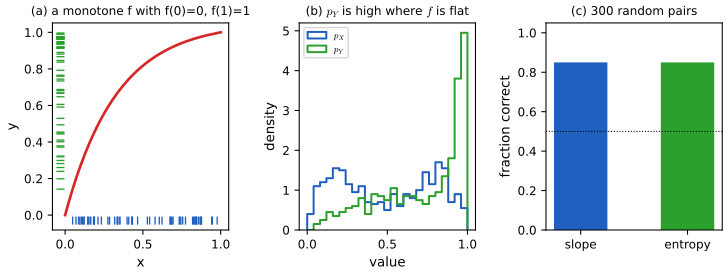
S30.5.2 Learning causal DAGs from interventional data
Supplement p. 265 Observational methods cannot separate Markov equivalent DAGs (gap 30.7). Interventional data, in which some variables have been set and the effects measured, can. For a perfect intervention (a variable is set deterministically), modify the likelihood-based method of S30.3: when computing the counts \(N_{ijk}=\sum_nI(X_{ni}=j,\bm X_{n,\pa(i)}=k)\) for node \(i\), leave out the cases \(n\) in which \(X_i\) was set from outside rather than drawn from \(\theta_{ijk}\) [CY99]; this is Bayesian parameter inference on a set of "mutilated" models with shared parameters. Real experiments rarely control one variable ("fat hand" interventions that touch several): model the interventions as extra nodes with no edges between them and none from regular nodes into them, and learn the larger augmented DAG. Dealing with the flow cytometry data of [Sac+05] this way (median graph of edges with posterior probability above 0.5, by the exact algorithm of [Koi06; EM07]) is Main Figure 20.7. To choose the best interventions with little data is active learning or experimental design [Mur01; HG09; KB14; HB14; Mue+17].
Filling the gap 30.18: why the counts omit the intervened cases, and why interventions break Markov equivalence Supplement p. 265
Proof
(i) The mutilated likelihood. Under a perfect intervention \(\mathrm{do}(X_i=x)\) the mechanism of node \(i\) is replaced by the constant \(x\) and all the others are unchanged (truncated factorisation): the density of a case is \(\prod_{t\ne i}p(x_t\given\bm x_{\pa(t)},\theta_t)\) with \(x_i=x\) fixed. So the log-likelihood of an intervened case has no term for node \(i\): in the counts \(N_{tck}\) of node \(i\)'s own family (but not of its children's families, in which \(X_i\) appears only as a parent) the case does not count. Since the parameters \(\theta_{tc}\) are shared between observational and interventional cases and the priors are the same Dirichlets, the integrals factorise as in gap 30.8 with the modified counts; the formula (S30.26) and BDeu are used unchanged.
(ii) Interventions separate the two orientations. Take binary \(X,Y\) with true model \(X\to Y\). With observational data BDeu gives equal scores to \(X\to Y\) and \(Y\to X\) (gap 30.8(iii); confirmed to 1e-9), so \(p(X\to Y\given\mathcal D)=\tfrac12\) whatever \(N\) is. Now let half of the cases set \(X\) by an intervention. Under \(X\to Y\) the intervened cases still inform \(p(y\given x)\) and are left out only of the marginal \(p(x)\); under \(Y\to X\) the intervened cases are left out of \(p(x\given y)\) but enter \(p(y)\), which in that model cannot depend on the value set for \(X\) (in the mutilated model \(Y\) is a root), whereas in the data the distribution of \(Y\) in the intervened cases clearly depends on the value set. A single \(p(y)\) fitted to a mixture of two different laws loses in likelihood a term proportional to the number of intervened cases (a Jensen-gap between \(p(y\given x=0)\) and \(p(y\given x=1)\)), so the Bayes factor for \(X\to Y\) grows exponentially in \(N\). In Figure x30.4 the posterior of the true direction goes from 0.5 (observational data only) to 0.76 at \(N=20\), 0.99 at \(N=200\) and 1.00 at \(N=1000\) with half of the cases intervened, in 40 repetitions per \(N\).
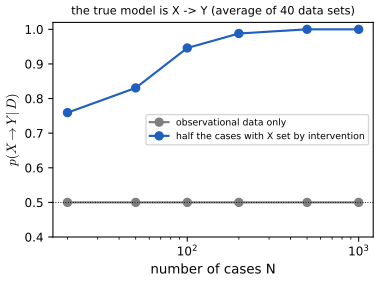
S30.5.3 Learning from low-level inputs
Supplement pp. 265–266 Often the data are low level (pixels) and are generated by higher-level latent causal factors (objects interacting in a scene). Learning such models is causal representation learning: causal discovery combined with latent variable models such as VAEs (Chapter 21) and representation learning (Murphy 2023, Chapter 32); see [CEP17; Sch+21].
Practice problems
The book has no end-of-chapter exercises for Chapter 30, so here are three short problems of my own, with complete solutions (hidden).
Practice problem 30.1 (Chow-Liu on a Markov chain). Three binary variables form a Markov chain \(x_1\to x_2\to x_3\) with \(p(x_1=1)=\tfrac12\), \(x_2\) equal to \(x_1\) with probability 0.9, and \(x_3\) equal to \(x_2\) with probability 0.8. (a) Compute the three pairwise mutual informations (in nats). (b) Which tree does the Chow-Liu algorithm return from the exact distribution? (c) Show that for any Markov chain the weight of the "skip" edge \((1,3)\) is smaller than the weights of both chain edges, so the true chain is recovered.
Solution
(a) By symmetry each variable is uniform, and for a binary symmetric channel with flip probability \(\epsilon\), \(I=\log2-h(\epsilon)\) with \(h(\epsilon)=-\epsilon\log\epsilon-(1-\epsilon)\log(1-\epsilon)\). Then \(I(x_1;x_2)=\log2-h(0.1)=0.6931-0.3251=0.3681\) and \(I(x_2;x_3)=\log2-h(0.2)=0.6931-0.5004=0.1927\). The variable \(x_3\) differs from \(x_1\) with probability \(0.1\cdot0.8+0.9\cdot0.2=0.26\), so \(I(x_1;x_3)=\log2-h(0.26)=0.6931-0.5731=0.1201\). (The values from a direct computation on the joint table are 0.36806, 0.19274 and 0.12009.) (b) The maximum weight spanning tree takes the two heaviest edges, \((1,2)\) and \((2,3)\), whose union is a tree: the true chain (the third edge would close a cycle). (c) By the data processing inequality for the chain \(x_1\to x_2\to x_3\), \(I(x_1;x_3)\le I(x_1;x_2)\) and, applying it to the reversed chain \(x_3\to x_2\to x_1\), \(I(x_1;x_3)\le I(x_2;x_3)\). So the weight of the skip edge is at most the smaller of the chain weights; with strict inequality (as here) Kruskal always rejects it. This is why Chow-Liu recovers the structure of any tree-structured distribution in the limit \(N\to\infty\).
Practice problem 30.2 (counting DAGs and equivalence classes on three nodes). How many DAGs are there on three labelled nodes, and how many Markov equivalence classes? List the classes by skeleton.
Solution
Count by skeleton. No edges: 1 DAG, 1 class. One edge (3 skeletons): 2 orientations each, 6 DAGs, and the two orientations are equivalent (no v-structure possible): 3 classes. Two edges (a path, 3 skeletons): 4 orientations each, 12 DAGs; the three orientations without a collider (chain either way, fork) form one class and the collider is a second class: 6 classes. Three edges (the triangle): the acyclic orientations are the \(3!=6\) transitive tournaments; every v-structure would need two non-adjacent parents, but all pairs are adjacent, so there are no v-structures and the 6 DAGs form 1 class. Totals: \(1+6+12+6=25\) DAGs (Robinson's \(a_3=25\)) and \(1+3+6+1=11\) classes, as brute-force enumeration confirms (the counts of classes for 1, 2, 3, 4, 5 nodes are 1, 2, 11, 185, 8782).
Practice problem 30.3 (the graphical lasso for two variables). Let \(\bm S=\begin{pmatrix}1&s\\s&1\end{pmatrix}\) with \(s>0\). Using the optimality conditions of gap 30.15 (diagonal penalised), find the solution of S(30.50) in closed form, show that an edge is present iff \(s>\lambda\), and evaluate \(\hat{\bm\Omega}\) for \(s=0.6\), \(\lambda=0.2\).
Solution
The covariance estimate starts at \(\bm W=\bm S+\lambda\bm I\) with \(W_{11}=W_{22}=1+\lambda\). The regression of node 2 on node 1 is a scalar lasso with Gram value \(W_{11}=1+\lambda\) and cross-product \(s\): \(\beta=\mathrm{soft}(s,\lambda)/(1+\lambda)\), which is non-zero iff \(s>\lambda\). Hence the off-diagonal \(\hat\Omega_{12}=-\beta\hat\Omega_{22}\) is non-zero iff \(s>\lambda\): an edge appears exactly when the sample correlation exceeds the penalty (the rule \(\lambda\ge\max|S_{jk}|\) of gap 30.15 for \(D=2\)). Then \(w_{12}=W_{11}\beta=s-\lambda\), \(\hat\Omega_{22}=1/(w_{22}-w_{12}\beta)=1/\big(1+\lambda-(s-\lambda)^2/(1+\lambda)\big)\) and, by symmetry, \(\hat\Omega_{11}=\hat\Omega_{22}\). For \(s=0.6\), \(\lambda=0.2\): \(\beta=0.4/1.2=\tfrac13\), \(w_{12}=0.4\), \(\hat\Omega_{22}=1/(1.2-0.1333)=0.9375\) and \(\hat\Omega_{12}=-0.3125\). The code (
glasso) returns \(\begin{pmatrix}0.9375&-0.3125\\-0.3125&0.9375\end{pmatrix}\) and the covariance \(\bm W=\begin{pmatrix}1.2&0.4\\0.4&1.2\end{pmatrix}\), whose inverse it is; for \(\lambda=0.7\) (above \(s\)) it returns no edge.
Demonstrations
- The graphical lasso path (Figure 30.1, Section S30.4.2): the flow cytometry covariance, two simulated chains and the example (S30.48); move \(\lambda\) and watch the edges and the partial correlations.
- The PC algorithm and Markov equivalence (Section S30.3.5): three true DAGs, the oracle or Fisher z tests, the number of cases and the test level; the output against the true essential graph.
- Which way does the arrow point? (Section S30.5.1): additive noise models tested with HSIC in both directions, plus the IGCI slope and entropy rules, on four data sets.
Python code for every figure: code index. Data used by the demos: data/ch30-glasso.json, data/ch30-pc.json, data/ch30-pairs.json, data/ch30-sachs.json. Companion demos: Gaussian graphical models (Chapter 4), All of Statistics (graphs, causal inference).
Notes on the book
Points where the book (mostly the supplement) is imprecise or wrong
- S(30.33). \(h(\bm W)=\Tr(\bm I+\alpha\bm W)^D-D\) does not characterise DAGs for a matrix \(\bm W\) with entries of both signs: closed walks with opposite signs cancel in the trace (a cyclic \(\bm W\) with \(h=0\) is given in gap 30.11). The entries must be squared, \(\bm W\circ\bm W\), as in the original paper.
- Section S30.5.1.5. "An IGCI model satisfies \(H(X)\le H(Y)\)": the sign is reversed. By change of variables \(H(Y)=H(X)+\E\log f'(X)\), and under IGCI \(\E\log f'(X)=\int\log f'\le0\) (Jensen), so \(H(Y)\le H(X)\) (gap 30.17); the direction is chosen by \(H(X)>H(Y)\). The sentence about \(p_Y\) being "less uniform" is consistent with the correct sign.
- S(30.49). The worked example prints \(\hat\Omega_{22}=0.11\); the constrained MLE has \(\hat\Omega_{22}=0.1048\), which rounds to 0.10 (the other entries agree).
- S(30.53)–S(30.54). The text indexes the means by \(\mu_x\) in the first form and by \(\mu_1,\mu_2\) in the second; and \(\alpha=\mathrm{logit}(\theta)+(\mu_0^2-\mu_1^2)/2\) needs the factor \(\tfrac12\), lost in the draft (gap 30.16(i)).
- S(30.30). The BIC penalty is written \(K_tC_t/2\log N\); a CPT has \(C_t(K_t-1)\) free parameters, so the penalty should be \(C_t(K_t-1)/2\cdot\log N\).
- S(30.31). The recurrence is stated "for \(D>2\)" with base case \(f(1)=1\); it holds for all \(D\ge1\) with \(f(0)=1\) (it gives \(f(2)=3\)), and the claim in the footnote that the numbers equal the number of \((0,1)\) matrices with positive real eigenvalues is a separate theorem [McK+04].
- Footnote 4 (Section S30.4.4). The number of decomposable graphs on 7 nodes is printed "61,7675"; it is 617,675 (checked by enumeration up to 6 nodes: 2, 8, 61, 822, 18 154).
- Sections S30.3.7 and S30.3.8.6. "The MAP converges to the MLE, which converges to the true graph" omits the argument (gap 30.12: faithfulness, I-maps and the minimal parameter count); and S(30.44) writes the structural EM inequality with the expected-data and observed-data score differences in the wrong order (the guaranteed direction is the one proved in gap 30.13(iv)).
- Section S30.3.8.4. "One can prove that the variational bound is always more accurate than CS, which is always more accurate than BIC": for small samples BIC is on average close to the exact value but very variable, and CS was less accurate than the variational bound in my experiment (Figure x30.2); I would read the statement as an empirical finding of [BG06], not as a theorem.
References
Keys in square brackets are the ones used in the book and its supplement.
- Murphy, K. P. (2023). Probabilistic Machine Learning: Advanced Topics. MIT Press, Cambridge, MA. Chapter 30, pp. 1043–1045, and supplementary material, Chapter 30. probml.github.io/pml-book/book2.html.
- [Air+08] Airoldi, E. M., Blei, D. M., Fienberg, S. E. and Xing, E. P. (2008). Mixed membership stochastic blockmodels. Journal of Machine Learning Research, 9, 1981–2014.
- [Ana+14] Anandkumar, A., Ge, R., Hsu, D., Kakade, S. M. and Telgarsky, M. (2014). Tensor decompositions for learning latent variable models. Journal of Machine Learning Research, 15, 2773–2832.
- [BG06] Beal, M. J. and Ghahramani, Z. (2006). Variational Bayesian learning of directed graphical models with hidden variables. Bayesian Analysis, 1(4), 793–832.
- [CH92] Cooper, G. F. and Herskovits, E. (1992). A Bayesian method for the induction of probabilistic networks from data. Machine Learning, 9, 309–347.
- [Chi96] Chickering, D. M. (1996). Learning Bayesian networks is NP-complete. In Learning from Data: Artificial Intelligence and Statistics V. Springer. [Chi02] Chickering, D. M. (2002). Optimal structure identification with greedy search. Journal of Machine Learning Research, 3, 507–554. Chickering, D. M. (1995). A transformational characterization of equivalent Bayesian network structures. Uncertainty in Artificial Intelligence.
- [CL68] Chow, C. K. and Liu, C. N. (1968). Approximating discrete probability distributions with dependence trees. IEEE Transactions on Information Theory, 14(3), 462–467.
- [CS96] Cheeseman, P. and Stutz, J. (1996). Bayesian classification (AutoClass): theory and results. In Advances in Knowledge Discovery and Data Mining. AAAI Press.
- [CY99] Cooper, G. F. and Yoo, C. (1999). Causal discovery from a mixture of experimental and observational data. Uncertainty in Artificial Intelligence.
- [Dan+10] Daniusis, P., Janzing, D., Mooij, J., Zscheischler, J., Steudel, B., Zhang, K. and Schölkopf, B. (2010). Inferring deterministic causal relations. Uncertainty in Artificial Intelligence. [Jan+12] Janzing, D., Mooij, J., Zhang, K., Lemeire, J., Zscheischler, J., Daniusis, P., Steudel, B. and Schölkopf, B. (2012). Information-geometric approach to inferring causal directions. Artificial Intelligence, 182–183, 1–31.
- [Dem72] Dempster, A. P. (1972). Covariance selection. Biometrics, 28(1), 157–175.
- Darmois, G. (1953). Analyse générale des liaisons stochastiques. Revue de l'Institut International de Statistique, 21, 2–8. Skitovich, V. P. (1953). On a property of the normal distribution. Doklady Akademii Nauk SSSR, 89, 217–219.
- [FHT08] Friedman, J., Hastie, T. and Tibshirani, R. (2008). Sparse inverse covariance estimation with the graphical lasso. Biostatistics, 9(3), 432–441.
- [FK03] Friedman, N. and Koller, D. (2003). Being Bayesian about network structure: a Bayesian approach to structure discovery in Bayesian networks. Machine Learning, 50, 95–125.
- [Fri97] Friedman, N. (1997). Learning belief networks in the presence of missing values and hidden variables. International Conference on Machine Learning. [Thi+98] Thiesson, B., Meek, C., Chickering, D. M. and Heckerman, D. (1998). Learning mixtures of DAG models. Uncertainty in Artificial Intelligence.
- [GH94] Geiger, D. and Heckerman, D. (1994). Learning Gaussian networks. Uncertainty in Artificial Intelligence. [GH97] Geiger, D. and Heckerman, D. (1997). A characterization of the Dirichlet distribution through global and local parameter independence. Annals of Statistics, 25(3), 1344–1369.
- [Gre+05] Gretton, A., Bousquet, O., Smola, A. and Schölkopf, B. (2005). Measuring statistical dependence with Hilbert-Schmidt norms. Algorithmic Learning Theory.
- [GZS19] Glymour, C., Zhang, K. and Spirtes, P. (2019). Review of causal discovery methods based on graphical models. Frontiers in Genetics, 10, 524.
- [Hec+00] Heckerman, D., Chickering, D. M., Meek, C., Rounthwaite, R. and Kadie, C. (2000). Dependency networks for inference, collaborative filtering, and data visualization. Journal of Machine Learning Research, 1, 49–75.
- [HGC95] Heckerman, D., Geiger, D. and Chickering, D. M. (1995). Learning Bayesian networks: the combination of knowledge and statistical data. Machine Learning, 20, 197–243. [HMC97] Heckerman, D., Meek, C. and Cooper, G. (1997). A Bayesian approach to causal discovery. Microsoft Research Technical Report MSR-TR-97-05.
- [Hoy+09] Hoyer, P. O., Janzing, D., Mooij, J., Peters, J. and Schölkopf, B. (2009). Nonlinear causal discovery with additive noise models. Advances in Neural Information Processing Systems, 21.
- [HTF09] Hastie, T., Tibshirani, R. and Friedman, J. (2009). The Elements of Statistical Learning, 2nd edition. Springer (see also ESL Chapter 17 on this site). Haughton, D. (1988). On the choice of a model to fit data from an exponential family. Annals of Statistics, 16(1), 342–355.
- [HW11] Harmeling, S. and Williams, C. K. I. (2011). Greedy learning of binary latent trees. IEEE Transactions on Pattern Analysis and Machine Intelligence, 33(6), 1087–1097. [Cho+11] Choi, M. J., Tan, V. Y. F., Anandkumar, A. and Willsky, A. S. (2011). Learning latent tree graphical models. Journal of Machine Learning Research, 12, 1771–1812.
- [JHS13] Jernite, Y., Halpern, Y. and Sontag, D. (2013). Discovering hidden variables in noisy-or networks using quartet tests. Advances in Neural Information Processing Systems, 26. [Aro+16] Arora, S., Ge, R., Ma, T. and Risteski, A. (2016). Provable learning of noisy-or networks. arXiv:1612.08795.
- [JS10] Janzing, D. and Schölkopf, B. (2010). Causal inference using the algorithmic Markov condition. IEEE Transactions on Information Theory, 56(10), 5168–5194.
- [Kem+06] Kemp, C., Tenenbaum, J. B., Griffiths, T. L., Yamada, T. and Ueda, N. (2006). Learning systems of concepts with an infinite relational model. AAAI.
- [Koi06] Koivisto, M. (2006). Advances in exact Bayesian structure discovery in Bayesian networks. Uncertainty in Artificial Intelligence. [KS04] Koivisto, M. and Sood, K. (2004). Exact Bayesian structure discovery in Bayesian networks. Journal of Machine Learning Research, 5, 549–573.
- [Lac+20] Lachapelle, S., Brouillard, P., Deleu, T. and Lacoste-Julien, S. (2020). Gradient-based neural DAG learning. International Conference on Learning Representations.
- [Mee95] Meek, C. (1995). Causal inference and causal explanation with background knowledge. Uncertainty in Artificial Intelligence.
- [MB06] Meinshausen, N. and Bühlmann, P. (2006). High-dimensional graphs and variable selection with the lasso. Annals of Statistics, 34(3), 1436–1462. [Mei05] Meinshausen, N. (2005). A note on the lasso for Gaussian graphical model selection. Technical report, ETH Zürich.
- [MJ00] Meilă, M. and Jordan, M. I. (2000). Learning with mixtures of trees. Journal of Machine Learning Research, 1, 1–48. [MJ06] Meilă, M. and Jaakkola, T. (2006). Tractable Bayesian learning of tree belief networks. Statistics and Computing, 16, 77–92.
- [Moo+16] Mooij, J. M., Peters, J., Janzing, D., Zscheischler, J. and Schölkopf, B. (2016). Distinguishing cause from effect using observational data: methods and benchmarks. Journal of Machine Learning Research, 17, 1–102.
- [NS01] Nowicki, K. and Snijders, T. A. B. (2001). Estimation and prediction for stochastic blockstructures. Journal of the American Statistical Association, 96(455), 1077–1087.
- [Pea09] Pearl, J. (2009). Causality, 2nd edition. Cambridge University Press. [PJS17] Peters, J., Janzing, D. and Schölkopf, B. (2017). Elements of Causal Inference. MIT Press. Peters, J. and Bühlmann, P. (2014). Identifiability of Gaussian structural equation models with equal error variances. Biometrika, 101(1), 219–228.
- [Rob73] Robinson, R. W. (1973). Counting labeled acyclic digraphs. In New Directions in the Theory of Graphs, Academic Press, 239–273.
- [Sac+05] Sachs, K., Perez, O., Pe'er, D., Lauffenburger, D. A. and Nolan, G. P. (2005). Causal protein-signaling networks derived from multiparameter single-cell data. Science, 308(5721), 523–529.
- [SG91] Spirtes, P. and Glymour, C. (1991). An algorithm for fast recovery of sparse causal graphs. Social Science Computer Review, 9(1), 62–72. [SGS00] Spirtes, P., Glymour, C. and Scheines, R. (2000). Causation, Prediction, and Search, 2nd edition. MIT Press. [VP90] Verma, T. and Pearl, J. (1990). Equivalence and synthesis of causal models. Uncertainty in Artificial Intelligence.
- [Shi+06] Shimizu, S., Hoyer, P. O., Hyvärinen, A. and Kerminen, A. (2006). A linear non-Gaussian acyclic model for causal discovery. Journal of Machine Learning Research, 7, 2003–2030.
- [Zhe+18] Zheng, X., Aragam, B., Ravikumar, P. and Xing, E. P. (2018). DAGs with NO TEARS: continuous optimization for structure learning. Advances in Neural Information Processing Systems, 31.
The numerical statements in the text (the collapsed block-model likelihood and its sampler on the ring example; the Chinese restaurant prior; the Chow-Liu likelihood identity, optimality over all trees, and the forest, matrix-tree and edge-marginal results; the Markov equivalence theorem on all four-node DAGs and the counts of DAGs and classes; the faithfulness cancellation; the Dirichlet marginal likelihood, BDeu likelihood equivalence and the failure of the Jeffreys prior; the exact posterior over all five-node DAGs and local optimality of hill climbing; the PC algorithm with an oracle and with Fisher z tests; the Gaussian MLE of the worked example, the gradient, the glasso optimality conditions, scikit-learn agreement and the edge counts of Figure 30.1; the acyclicity function, its gradient and the counterexample; NOTEARS recovery; the exact latent class marginal likelihood against Monte Carlo and the three approximations; the structural EM inequality; the additive noise tests, the IGCI identities and the interventional scores; the counts of decomposable graphs) were confirmed numerically.