Autoregressive models
An autoregressive model (ARM) writes the joint distribution of a sequence by the chain rule, \(p(x_{1:T})=\prod_t p(x_t\given x_{1:t-1})\), and puts all its modelling effort into the conditionals. Because every factor is a normalised distribution, the likelihood is exact and cheap to evaluate and to maximise; sampling is sequential. The chapter goes through the ways to parametrise the conditionals: Markov truncation, the neural autoregressive density estimator (NADE) and the masked autoencoder (MADE), causal and dilated convolutions (WaveNet, PixelCNN), and causal self-attention (GPT and the large language models). These notes prove that each architecture really is autoregressive, count what each design costs, locate the PixelCNN blind spot exactly, solve the linear Gaussian ARM in closed form, and tie perplexity to code length.
Ch. 1 Introduction Ch. 2 Probability Ch. 3 Statistics Ch. 4 Graphical models Ch. 5 Information theory Ch. 6 Optimisation Ch. 7 Inference algorithms Ch. 8 Gaussian filtering Ch. 9 Message passing Ch. 10 Variational inference Ch. 11 Monte Carlo Ch. 12 MCMC Ch. 13 Sequential Monte Carlo Ch. 14 Predictive models Ch. 15 GLMs Ch. 16 Deep networks Ch. 17 Bayesian neural networks Ch. 18 Gaussian processes Ch. 19 Beyond iid Ch. 20 Generative models Ch. 21 VAEs Ch. 22 Autoregressive models Ch. 23 Normalizing flows Ch. 24 Energy-based models Ch. 25 Diffusion models Ch. 26 GANs Ch. 27 Discovery methods Ch. 28 Latent factor models Ch. 29 State-space models Ch. 30 Graph learning Ch. 31 Nonparametric Bayes Ch. 32 Representation learning Ch. 33 Interpretability Ch. 34 Decision making Ch. 35 Reinforcement learning Ch. 36 Causality
How to read these notes
They follow the book. Sections carry the book's numbers, and equations the book numbers keep their numbers, e.g. \((22.1)\); equations without a number are steps the book skips. The online supplement for this chapter has only a title page (see Supplement Chapter 22).
Filling the gaps. The chapter is a short survey and states its architectural claims (the model is autoregressive, a dilated stack sees far into the past, the mask removes the dependence on the future, transformers train in parallel) without proof. Each gets an orange Filling the gap box with the full argument. Proofs start hidden: open one with its bar, or use the buttons below. Results proved elsewhere on the site (the chain rule of probability, entropy and cross-entropy, the maximum-likelihood identities, the Gaussian conditioning formulas) are stated and linked rather than repeated.
Figures and demonstrations. The chapter's figures are diagrams (22.1 to 22.3), quotations of model output (22.4, 22.5) and samples of models with billions of parameters (22.6), so none is reproduced. Three figures of my own (22.x1 to 22.x3) illustrate results proved here; the Python code makes all of them. They are computed on small problems: a simulated binary source, the 8 × 8 digits data set bundled with scikit-learn, and exact enumerations. The ▶ Demo boxes open an interactive page set to the case being discussed.
Main reference
K. P. Murphy, Probabilistic Machine Learning: Advanced Topics, MIT Press (2023; online draft of December 2025), Chapter 22, pages 821–828 (book page: probml.github.io/pml-book/book2.html), and the supplementary material, Chapter 22, pages 199–200. Section, equation and figure numbers below refer to this book. The explanations, derivations, figures and code are my own. The book has no end-of-chapter exercises for Chapter 22; the practice problems at the end are mine.
Companion courses
Volume 1 treats the same models at an introductory level: Chapter 15 has RNNs with teacher forcing, causal 1d CNNs and transformers, and Section 6.1.5 defines perplexity. The deep-learning course covers autoregressive models and transformer language models in its Chapter 12, with a character-level transformer demo. Within this course, Section 16.3.4 and 16.3.5 introduce RNNs and transformers, Chapter 20 places ARMs among generative models, and Section 21.5.3 shows that an autoregressive model is a VAE with a trivial latent.
What this chapter adds: the proof that the chain rule gives a normalised density for any conditionals and for any ordering; why more context costs more data (with a source whose conditional entropy is known exactly); the MADE mask proof and the path matrix; the exact linear Gaussian ARM and its Cholesky structure; the receptive field of a dilated stack and the exact size of the PixelCNN blind spot; causal attention and its cost with and without a cache; perplexity as code length.
The chapter at a glance
- 22.1 Chain rule gives a valid joint for any conditionals and any order (gap 22.1); order-k Markov models, parameters and overfitting (22.2).
- 22.2 NADE recurrence and MADE masks (gap 22.3); the linear Gaussian ARM (22.4).
- 22.3 Dilated causal convolutions (gap 22.5); the PixelCNN blind spot (22.6).
- 22.4 Causal attention, parallel training, cost of sampling (gap 22.7).
- 22.5 Perplexity and compression (gap 22.8).
Notation. \(x_{1:t}=(x_1,\dots,x_t)\); \(x_{<t}=x_{1:t-1}\); \(h_2(p)=-p\log_2p-(1-p)\log_2(1-p)\) is the binary entropy in bits; \(\oplus\) is addition modulo 2; \(\mathrm{PP}\) is perplexity.
Prerequisites. Chapters 2 and 5 of the book, and Chapter 15 of Volume 1.
22.1 Introduction
pp. 821–822 By the chain rule of probability any joint distribution of \(T\) variables factorises as \[ p(x_{1:T})=p(x_1)p(x_2\given x_1)p(x_3\given x_{1:2})\cdots=\prod_{t=1}^Tp(x_t\given x_{1:t-1}), \tag{22.1} \] with \(p(x_1\given x_{1:0})=p(x_1)\). A model of this form is an autoregressive model (ARM). In graphical-model language it is the fully connected directed graph in which each node has all earlier nodes as parents (Figure 22.1, a diagram). The conditionals may also depend on a context \(c\), which is left implicit. The reverse ordering gives the "anti-causal" factorisation \[ p(x_{1:T})=\prod_{t=T}^{1}p(x_t\given x_{t+1:T}). \tag{22.2} \] Both are exact for the true distribution; which is easier to learn depends on the family used for the conditionals (gap 22.1).
Each factor depends on more and more arguments, so the unrestricted conditionals are costly and need a lot of data. Three ways out are described: (i) the first-order Markov assumption \(p(x_t\given x_{1:t-1})=p(x_t\given x_{t-1})\) (an AR model of order 1), which is very restrictive; (ii) a hidden state \(z_t\) that summarises the past, deterministic in an RNN (Section 16.3.4) and stochastic in a hidden Markov model (Section 9.2); (iii) keep the general form (22.1) but let a neural network with a restricted architecture compute \(p(x_t\given x_{1:t-1})\), so that the compact summary of the past is learned implicitly. This chapter follows route (iii).
The strength of ARMs is that the exact likelihood of a sequence is computable and can be optimised directly; the weaknesses are that generation is inherently sequential and that the model has no compact latent representation of the data.
Filling the gap 22.1: the chain rule gives a valid density for any conditionals and any ordering, and training is cross-entropy pp. 821–822, (22.1), (22.2)
Proof
(a) Any conditionals give a normalised joint. Let \(q_t(\cdot\given x_{<t})\) be, for every history \(x_{<t}\), a probability mass function (or density) on \(\mathcal X\), chosen in any way whatsoever (a table, a logistic regression, a neural network). Define \(q(x_{1:T})=\prod_tq_t(x_t\given x_{<t})\). Summing over the last variable first, \[ \sum_{x_T}q(x_{1:T})=q(x_{1:T-1})\sum_{x_T}q_T(x_T\given x_{<T})=q(x_{1:T-1}), \] and repeating down to \(t=1\) gives \(\sum_{x_{1:T}}q(x_{1:T})=1\) (integrals and Fubini's theorem for densities). There is no partition function and no constraint between the factors: every conditional is normalised on its own, which is why ARMs have exact likelihoods. Confirmed numerically for random conditional tables of four binary variables.
(b) Every joint, in every ordering, can be written this way. Let \(p\) be any joint and \(\pi\) any permutation of \(\{1,\dots,T\}\). Define \(p(x_{\pi(t)}\given x_{\pi(1)},\dots,x_{\pi(t-1)})=p(x_{\pi(1:t)})/p(x_{\pi(1:t-1)})\) wherever the denominator is positive (and arbitrarily elsewhere). The product telescopes to \(p(x_{\pi(1:T)})=p(x_{1:T})\). So an unrestricted ARM is a universal model of discrete distributions, for each of the \(T!\) orderings. The ordering matters only through the class of conditionals allowed: a Markov model of order 1 is exact for a Markov chain in the forward order, and typically not exact in an arbitrary other order. Confirmed numerically on a random joint of four binary variables with the natural order and a shuffled order.
(c) Training. For data \(x^{(1)},\dots,x^{(N)}\) the average log-likelihood is \[ \frac1N\sum_n\log q_\theta(x^{(n)}_{1:T})=\frac1N\sum_n\sum_{t}\log q_{\theta,t}\big(x^{(n)}_t\given x^{(n)}_{<t}\big), \] which is minus the cross-entropy between the empirical distribution and the model. Every term uses the observed history, so all \(T\) conditionals can be computed at once (this is called teacher forcing, Volume 1, Section 15.2.4) if the architecture allows it. For a true distribution \(p\) the expected loss splits as \(\E_p[-\log q]=\Hent(p)+\Dkl(p\|q)\) and the KL divergence obeys a chain rule, obtained by telescoping the log ratio: \[ \Dkl(p\|q)=\sum_{t=1}^T\E_{x_{<t}\sim p}\,\Dkl\big(p(\cdot\given x_{<t})\,\|\,q_t(\cdot\given x_{<t})\big). \] So the whole sequence loss is the sum of the per-step conditional errors, each weighted by how often the history occurs.
(d) Cost. Evaluating \(q(x_{1:T})\) needs \(T\) conditionals, which are independent given the data. Drawing a sample needs \(x_{<t}\) before \(x_t\): \(T\) sequential steps, which cannot be parallelised across \(t\).
(e) The direction. The book says the anti-causal direction (22.2) is often harder to learn and cites Peters, Janzing and Schölkopf (2017). For a stationary Gaussian AR(1), \(x_t=\varphi x_{t-1}+e_t\), the forward and backward factorisations are both exact with the same form (the process is reversible): the log density of a draw is the same, to rounding error, in the two orders, and equals the multivariate normal log density. The asymmetry the book refers to appears for non-Gaussian noise and for restricted families, where the backward conditional is not "predictor plus independent noise"; that statement is quoted from the reference and not reproved here. \(\square\)
Filling the gap 22.2: Markov models, why more context costs more data, and a source where the answer is known p. 821 (the Markov assumption), Section 2.6.3.2
Proof
The model class. For binary data the order-\(k\) Markov model has \(p(x_t=1\given x_{t-k:t-1})=\theta_c\) for each of the \(2^k\) contexts \(c\), so it has \(2^k\) free parameters (plus a table for the first \(k\) symbols), against \(2^{t-1}\) for the unrestricted conditional at step \(t\). Fitting is counting: with \(n_{c,v}\) the number of times symbol \(v\) follows context \(c\), the maximum-likelihood estimate is \(\hat\theta_c=n_{c,1}/n_c\). A symmetric Dirichlet (Beta) prior with constant \(\alpha\) gives the predictive probability \((n_{c,v}+\alpha)/(n_c+2\alpha)\). The product of these sequential predictive probabilities over the data equals the Dirichlet-multinomial marginal likelihood \(\prod_c B(n_{c,1}+\alpha,n_{c,0}+\alpha)/B(\alpha,\alpha)\) (a Pólya urn identity; confirmed numerically), so smoothing is a Bayesian choice and not an ad hoc trick.
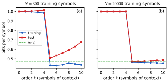
More context never hurts the population loss. For the best order-\(k\) conditional the expected log loss is the conditional entropy \(H_k=H(x_t\given x_{t-k:t-1})\), because \(\E[-\log q]=H+\Dkl\) and the KL term is zero for \(q\) equal to the true conditional. Conditioning cannot increase entropy: \(H_{k}-H_{k+1}=I(x_t;x_{t-k-1}\given x_{t-k:t-1})\ge0\). Hence \(H_0\ge H_1\ge\cdots\), with equality at step \(k\) exactly when \(x_t\) is conditionally independent of \(x_{t-k-1}\) given the nearer symbols. The same argument applied to the empirical distribution shows that the training log loss of the count-based maximum-likelihood fit is non-increasing in \(k\) (it is the empirical conditional entropy; confirmed numerically).
The test loss is not monotone. With \(2^k\) parameters and \(N\) observations the estimates are noisy when \(n_c\) is small: contexts seen once get probabilities 0 or 1, the training loss keeps falling (memorisation) and the test loss rises. This is the usual overfitting of maximum likelihood with many parameters.
A source with a known answer. Let \(x_0,\dots,x_4\) be fair coins and \(x_t=x_{t-2}\oplus x_{t-5}\oplus e_t\) with \(e_t\sim\mathrm{Ber}(\varepsilon)\) independent. Claim: for every \(t\ge5\) the window \((x_{t-5},\dots,x_{t-1})\) is uniform on \(\{0,1\}^5\). Induction: if the window is uniform, then given \((x_{t-4},\dots,x_{t-1})\) the symbol \(x_{t-5}\) is a fair coin independent of them and of \(e_t\), so \(x_t\) is a fair coin given \((x_{t-4},\dots,x_{t-1})\); hence \((x_{t-4},\dots,x_t)\) is uniform. Consequences: for \(k\le4\), \(x_t\) given the last \(k\) symbols is \(\mathrm{Ber}(1/2)\) (the missing \(x_{t-5}\) randomises it), so \(H_k=1\) bit; for \(k\ge5\), \(x_t\) given the last five symbols is \(x_{t-2}\oplus x_{t-5}\) flipped with probability \(\varepsilon\), so \(H_k=h_2(\varepsilon)\), which is 0.469 bits for \(\varepsilon=0.1\). On simulated data the order-4 test loss is 1.000 bits and the order-5 loss is 0.472 bits with \(N=20\,000\) (Figure 22.x1b), and a simulated residual \(x_t\oplus x_{t-2}\oplus x_{t-5}\) has flip rate 0.1004 in \(2\times10^5\) symbols. \(\square\)
See also: entropy and conditional entropy (Chapter 5), Dirichlet-multinomial estimation (Chapter 3), teacher forcing (Volume 1).
22.2 Neural autoregressive density estimators (NADE)
p. 822 A simple way to model each conditional is a generalised linear model such as logistic regression (Frey, 1998). A neural network makes it more powerful: the neural autoregressive density estimator (NADE; Larochelle and Murray, 2011). For real-valued data, letting each conditional be a mixture of Gaussians, \[ p(x_t\given x_{1:t-1})=\sum_{k=1}^K\pi_{t,k}\,\N(x_t\given\mu_{t,k},\sigma_{t,k}^2),\qquad(\bm\mu_t,\bm\sigma_t,\bm\pi_t)=f_t(x_{1:t-1};\theta_t), \tag{22.3} \] gives RNADE (Uria, Murray and Larochelle, 2013). Rather than \(T\) separate networks \(f_1,\dots,f_T\) it is more efficient to use one network with \(T\) inputs and \(T\) outputs and masking: the masked autoencoder for density estimation, MADE (Germain et al., 2015). A drawback of this family is that it needs a natural linear ordering, sensible for time series and not for images or graphs; orderless variants exist (Uria et al., 2014, 2016).
Whatever the parameters, (22.3) is a probability density in \(x_t\) (a convex combination of normal densities), so by gap 22.1(a) the product over \(t\) is a density in \(x_{1:T}\) and no further normalisation is needed.
Filling the gap 22.3: the NADE recurrence and why the MADE masks make a network autoregressive p. 822
Proof
NADE. Take binary data. Let the hidden pre-activation for the conditional of \(x_d\) be \(\bm a_d=\bm c+\sum_{j<d}\bm W_{:,j}x_j\in\R^H\) and let \(p(x_d=1\given x_{<d})=\sigma(b_d+\bm V_{d,:}^\T\sigma(\bm a_d))\). The weights \(\bm W\in\R^{H\times D}\) are tied across the conditionals (column \(j\) is used by every conditional that sees \(x_j\)). Then \(\bm a_{d+1}=\bm a_d+\bm W_{:,d}x_d\): each new pre-activation costs \(O(H)\) from the previous one, so the whole density costs \(O(DH)\) instead of \(O(D^2H)\), and the parameter count is \(2DH+H+D\) instead of \(H\,D(D-1)/2\) for untied first layers (for \(D=8,H=6\): 48 against 168 weights of the first layer). The recurrence agrees with the from-scratch computation to rounding error, and the probabilities of all \(2^8\) configurations of a random NADE sum to 1, as part (a) of gap 22.1 requires.
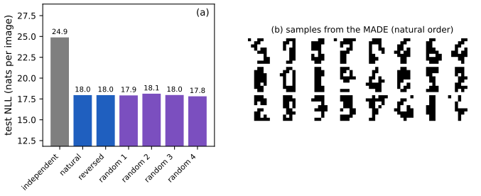
MADE. Give input \(d\) a position \(p_d\in\{1,\dots,D\}\) in the ordering (a permutation; \(x_d\) is modelled after all inputs with smaller position). Give each hidden unit \(j\) of each hidden layer \(\ell=1,\dots,L\) a degree \(m^\ell_j\in\{1,\dots,D-1\}\). Mask the weights of the ordinary network by \[ M^1_{jd}=\mathbb 1[m^1_j\ge p_d],\qquad M^\ell_{jk}=\mathbb 1[m^\ell_j\ge m^{\ell-1}_k]\ (\ell\ge2),\qquad M^{\rm out}_{dk}=\mathbb 1[p_d>m^L_k]. \] Claim. Hidden unit \(j\) of layer \(\ell\) depends only on inputs \(d\) with \(p_d\le m^\ell_j\), and output \(d\) depends only on inputs with \(p_{d'}<p_d\). Proof by induction on the layer. Layer 1: unit \(j\) is connected only to inputs with \(p_d\le m^1_j\). Step: unit \(j\) of layer \(\ell\) is connected only to units \(k\) of layer \(\ell-1\) with \(m^{\ell-1}_k\le m^\ell_j\), and each such unit depends only on inputs with \(p\le m^{\ell-1}_k\le m^\ell_j\). Output \(d\) is connected only to units with \(m^L_k<p_d\), which depend only on inputs with \(p\le m^L_k<p_d\). \(\square\) So the \(d\)-th output is a function of \(x_{\{d':p_{d'}<p_d\}}\) alone and may be taken as the parameters of \(p(x_d\given x_{\{d':p_{d'}<p_d\}})\); the product of the \(D\) outputs is a normalised density by gap 22.1(a). Confirmed numerically: the autograd Jacobian of the logits of a random 2-layer MADE with a shuffled ordering has non-zeros only where position \(p_{d'}<p_d\); the \(2^{10}\) probabilities of that network sum to 1; ancestral sampling reproduces the exact distribution of a small MADE (total variation 0.007 for 40 000 draws).
The path matrix. Multiplying the masks, \(P=M^{\rm out}M^L\cdots M^1\) has entry \(P_{dd'}\) equal to the number of paths from input \(d'\) to output \(d\); by the claim \(P_{dd'}=0\) unless \(p_{d'}<p_d\). Conversely, a pair with \(p_{d'}<p_d\) is connected as soon as some hidden degree lies in \([p_{d'},p_d-1]\) at every layer: take a chain of units all of degree \(m=p_{d'}\) (allowed, since \(m\ge p_{d'}\), \(m\ge m\) and \(p_d>m\)). With degrees \(1+(j\bmod(D-1))\) and \(H\ge D-1\) every earlier-to-later pair is connected, so the network is as expressive as the dependency pattern permits; with fewer hidden units some pairs have no path (demo preset 3). The unit of position 1 has no incoming connection at all: its conditional is the marginal of that variable, a bias only. Different orderings define different, equally valid models of the same data; training with many orderings sampled at random (and averaging) is the "orderless" extension. \(\square\)
Linear Gaussian autoregressions (own result)
The simplest ARM with real data replaces the network by a linear map: \(x_t\given x_{<t}\sim\N(\bm w_t^\T x_{<t},\,d_t)\). It is a useful reference point because everything is explicit.
Filling the gap 22.4: the linear Gaussian ARM is a Gaussian, with a Cholesky structure own result; relates to (22.1), (22.3)
Proof
The model is a multivariate normal. Let \(\bm B\) be strictly lower triangular with \(B_{t,1:t-1}=\bm w_t^\T\), \(\bm D=\diag(d_t)\) and \(\bm\epsilon\sim\N(\bm0,\bm D)\). The model says \(\bm x=\bm B\bm x+\bm\epsilon\), i.e. \((\bm I-\bm B)\bm x=\bm\epsilon\). Because \(\bm I-\bm B\) is unit lower triangular it is invertible with determinant 1, so \(\bm x\sim\N(\bm0,\bm\Sigma)\) with \[ \bm\Sigma=(\bm I-\bm B)^{-1}\bm D(\bm I-\bm B)^{-\T},\qquad \bm\Sigma^{-1}=(\bm I-\bm B)^\T\bm D^{-1}(\bm I-\bm B),\qquad \det\bm\Sigma=\prod_td_t. \] The change of variables \(\bm\epsilon=(\bm I-\bm B)\bm x\) has Jacobian 1, so \(\log p(\bm x)=\sum_t\log\N(x_t\given\bm w_t^\T x_{<t},d_t)\), the chain-rule sum, equals the multivariate normal log density. Confirmed numerically for a random \(5\times5\) covariance.
Every Gaussian is representable, in every ordering. For \(\bm\Sigma\succ0\) the LDL factorisation \(\bm\Sigma=\bm L\bm D\bm L^\T\), \(\bm L\) unit lower triangular, \(\bm D\) diagonal positive, is unique; set \(\bm I-\bm B=\bm L^{-1}\). So a linear Gaussian ARM represents any Gaussian exactly in any ordering (reordering the variables reorders \(\bm\Sigma\) and changes \(\bm B\) and \(\bm D\), not the density: the log density is the same to rounding error for a random permutation). The ordering therefore matters only for sparsity: if \(\bm\Sigma^{-1}\) is banded with half-bandwidth \(q\), the factor \(\bm I-\bm B\) in \(\bm\Sigma^{-1}=(\bm I-\bm B)^\T\bm D^{-1}(\bm I-\bm B)\) (a Cholesky factorisation of the precision matrix) is banded with the same half-bandwidth, because Cholesky factors of banded matrices have no fill-in outside the band. In particular a tridiagonal precision matrix gives \(x_t\) depending on \(x_{t-1}\) only (a first-order autoregression); checked numerically. The stationary AR(1) of gap 22.1(e) is this case. A neural ARM replaces \(\bm w_t^\T x_{<t}\) and \(d_t\) by networks; what the linear case shows is that the factorisation costs nothing in generality for exact families, and what it does not show (the interesting part of the chapter) is how to choose a restricted architecture that is both cheap and flexible. \(\square\)
22.3 Causal CNNs
p. 822 To represent \(p(x_t\given x_{1:t-1})\) one can look for patterns in the history that predict \(x_t\). If a pattern can occur anywhere, a convolution is natural, provided it only touches the past: a masked or causal convolution.
22.3.1 1d causal CNN (convolutional Markov models)
p. 823 The convolutional Markov model for a discrete sequence is \[ p(x_{1:T})=\prod_{t=1}^Tp(x_t\given x_{1:t-1};\theta)=\prod_{t=1}^T\Cat\Big(x_t\,\Big|\,\softmax\Big(\varphi\Big(\sum_{\tau=1}^{t-k}\bm w^\T x_{\tau:\tau+k}\Big)\Big)\Big), \tag{22.4} \] with a filter \(\bm w\) of size \(k\) and a single nonlinearity \(\varphi\) (see the note in Notes on the book about the index range). Deeper models and conditioning features can be added. To capture long-range dependence one uses dilated convolutions, which skip inputs with a stride \(d\) (Volume 1, Section 14.4.1). This is the WaveNet model of van den Oord et al. (2016a) for speech synthesis, a conditional model \(p(\bm x\given\bm c)\) with \(\bm c\) linguistic features and \(\bm x\) the raw audio waveform; Tacotron (Wang et al., 2017) is end-to-end from words. WaveNet is too slow for production but can be distilled into a parallel generative model (van den Oord et al., 2018; the book's Section 23.2.4.3). Figure 22.2 shows dilation factors 1, 2, 4, 8.
Filling the gap 22.5: causality and the receptive field of a dilated causal stack p. 823, Figure 22.2
Proof
Causal means shifted. A causal convolution of kernel size \(k\) and dilation \(d\), \(h_t=\varphi(\sum_{j=0}^{k-1}w_jh'_{t-jd})\), is an ordinary convolution after padding \((k-1)d\) zeros on the left, and \(h_t\) uses only inputs at times \(\le t\). A stack of such layers has the same property by induction: the output at \(t\) of layer \(\ell\) depends on layer-\((\ell-1)\) outputs at times \(t-j_\ell d_\ell\), \(j_\ell\in\{0,\dots,k-1\}\), all \(\le t\). So the stack defines \(p(x_{t+1}\given x_{1:t})\) from the inputs up to \(t\) only (an output head predicts the next symbol).
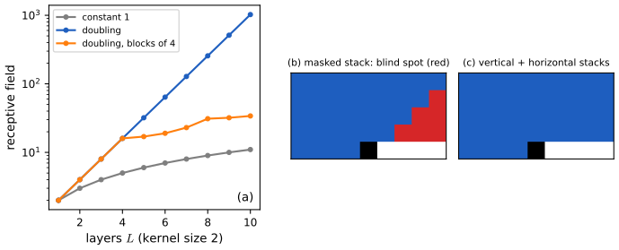
Receptive field. Unrolling the \(L\) layers, the output at time \(t\) depends exactly on the inputs at times \(t-\sum_{\ell=1}^Lj_\ell d_\ell\) over all choices \(j_\ell\in\{0,\dots,k-1\}\), so the oldest input seen is \(t-(k-1)\sum_\ell d_\ell\) and the receptive field (number of positions up to and including \(t\)) is at most \[ 1+(k-1)\sum_{\ell=1}^Ld_\ell, \] with equality in the sense of the oldest position reached (checked by propagating the dependency graph for several \((k,\bm d)\)). Without dilation (\(d_\ell=1\)) the field grows linearly in \(L\). Doubling: for \(k=2\) and \(d_\ell=2^{\ell-1}\) the reachable lags are \(\sum_\ell j_\ell2^{\ell-1}\) with \(j_\ell\in\{0,1\}\): the binary expansions of \(0,1,\dots,2^L-1\), each integer exactly once. So the field is the full window of \(2^L\) positions, with no gaps, and each input reaches the output by one unique path. Figure 22.2 (\(L=4\)): 16. For a sampling rate of 16 kHz one second is 16 000 samples, and \(L=14\) doubling layers give 16 384; the WaveNet recipe repeats the block \(1,2,\dots,512\) several times, and three blocks give \(3\cdot1023+1=3070\) positions (about 0.19 s at 16 kHz). For \(k=3\) and dilations \(3^{\ell-1}\) the reachable lags are all integers up to \(3^L-1\) (base-3 digits), so \(L=9\) layers give 19 683. \(\square\)
22.3.2 2d causal CNN (PixelCNN)
p. 823 The extension to images conditions each pixel on all earlier pixels in raster-scan order, \[ p(\bm x\given\theta)=\prod_{r=1}^R\prod_{c=1}^Cp\big(x_{r,c}\given f_\theta(\bm x_{1:r-1,1:C},\bm x_{r,1:c-1})\big), \tag{22.5} \] the PixelCNN (van den Oord et al., 2016b); Figure 22.3 shows the binary mask on the top-left context and the two-stack design that avoids blind spots (a vertical stack with all previous rows and a horizontal stack with the current row). Generating an image of \(N=RC\) pixels takes \(N\) sequential steps; Reed et al. (2017) use a multiscale approach to reduce the number of sequential steps to \(O(\log N)\) (see the note in Notes on the book). Extensions: PixelCNN++ (Salimans et al., 2017) uses a mixture of logistics for the multimodal conditional; PixelRNN (van den Oord, Kalchbrenner and Kavukcuoglu, 2016) combines masked convolution with an RNN; the Subscale Pixel Network (Menick and Kalchbrenner, 2019) samples high-order bits first, so that fine detail is conditioned on a low-resolution version of the whole image.
Filling the gap 22.6: mask A, mask B, and the exact size of the blind spot p. 823, Figure 22.3
Proof
Setup. Use offsets \((\Delta r,\Delta c)\) from the output pixel and let \(h=\lfloor k/2\rfloor\). A \(k\times k\) kernel covers \(|\Delta r|\le h\), \(|\Delta c|\le h\). Let \(\mathcal N=\{(\Delta r,\Delta c):\Delta r<0\text{ or }(\Delta r=0,\Delta c<0)\}\) be the raster-past. Mask A keeps the kernel offsets in \(\mathcal N\) (the centre is dropped); mask B keeps those in \(\mathcal N\cup\{(0,0)\}\). A stack of \(L\) masked convolutions (first layer A, the rest B) lets the output depend on the input at offset \(\bm\delta\) iff \(\bm\delta\) is a sum \(\bm\delta_1+\dots+\bm\delta_L\) of kernel offsets, one per layer, taken from the allowed sets.
Causality. The set \(\mathcal N\) is closed under addition (lexicographic order is compatible with addition), and \(\mathcal N\cup\{0\}\) too. A sum in which at least one term is in \(\mathcal N\) therefore lies in \(\mathcal N\): never the centre pixel and never a pixel in the future. That is why the first layer must be mask A; if it were mask B the all-zero choice would put the centre pixel (the value being predicted) in the receptive field.
The reach. Which \(\bm\delta\in\mathcal N\) are sums? Upper bound on the right. A layer that moves up (\(\Delta r\le-1\)) can move right by at most \(h\); a layer that stays in the row (\(\Delta r=0\)) can only move left or stay (\(\Delta c\le0\)). To reach row \(-j\) the number of layers that move up is at most \(\min(j,L)\) (each decreases the row by at least 1), so the column is at most \(h\min(j,L)\). The rows reached satisfy \(j\le Lh\), the columns \(|\Delta c|\le Lh\). Everything else is reached (construct the layers: for \(1\le j\le Lh\) take \(n=\min(j,L)\) layers that move up, with row steps in \([1,h]\) summing to \(j\), possible since \(n\le j\le nh\); put the first, mask-A, layer among them; give them column steps in \([-h,h]\) summing to the target \(m\) with \(m\le hn\); let the other layers stay at \((0,0)\) with mask B; negative columns down to \(-Lh\), and the current row to the left, are reached the same way). So \[ \text{reached}=\{(-j,m):1\le j\le Lh,\ -Lh\le m\le h\min(j,L)\}\ \cup\ \{(0,m):-Lh\le m\le-1\}, \] and the blind spot, the raster-past pixels inside the box \(|\Delta r|\le Lh,|\Delta c|\le Lh\) that the output can never see, is \[ \{(-j,m):\ h\min(j,L)<m\le Lh\},\qquad \#=\sum_{j=1}^{Lh}\big(Lh-h\min(j,L)\big)=\frac{h\,L(L-1)}2 . \] For \(j\ge L\) the term vanishes, and \(\sum_{j=1}^L(Lh-hj)=hL(L-1)/2\). A single layer has no blind spot (\(L=1\)); for \(k=3\) the blind spot has \(0,1,3,6,10\) pixels for \(L=1,\dots,5\); for \(k=5\), \(L=3\) it has 6 and for \(k=7\), \(L=5\) it has 30. The formula was confirmed by propagating the sets for \(k=3,5,7\) and \(L=1,\dots,5\), and the picture of the reach (Figure 22.x3b) is the exact set for \(k=3\), \(L=4\) (6 red pixels, the top-right triangle).
The two-stack remedy. The vertical stack is an ordinary (not column-masked) convolution over the rows above the current one, so its output at a pixel sees a full rectangle of rows above with columns \(\pm h\) per layer; the horizontal stack adds the current row to the left and receives the vertical stack's output from the row above (shifted down by one, so that no value from the current row leaks). The union is the whole box of raster-past pixels: no blind spot (Figure 22.x3c; the bookkeeping of the exact first-layer offsets, which the book leaves to the reference, only changes the box by a row). \(\square\)
See also: causal 1d CNNs for sequence generation (Volume 1) and convolutional networks (deep-learning course).
22.4 Transformers
p. 824 Transformers (Section 16.3.5 of the book; notes) can encode sequences (BERT), decode them, or do both in an encoder-decoder for conditional generation \(p(y\given c)\). Alternatively one defines a joint sequence model \(p(c,y)\) and conditions on the prompt \(c\) by feeding it as the initial context.
The decoder works as follows. At step \(t\) it applies masked (causal) self-attention (Section 16.2.7) to the first \(t\) inputs \(y_{1:t}\), computing attention weights \(a_{1:t}\) and an activation \(\bm z_t=\sum_{\tau\le t}a_{t,\tau}\bm y_\tau\) (see the note on the printed indices in Notes on the book), which goes through a feed-forward layer, \(\bm h_t=\mathrm{MLP}(\bm z_t)\); this repeats in every layer, and the last layer predicts the next element, \(y_{t+1}\sim\Cat(\softmax(\bm W\bm h_t))\). At training time all predictions happen in parallel, because the target sequence is known: the output at position \(t\) predicts \(y_{t+1}\) from \(y_{1:t}\) for all \(t\) at once. At test time the model must be applied sequentially, feeding each generated element back in. The running time is \(O(T^2)\), and many more efficient variants exist (Volume 1, Section 15.6).
Filling the gap 22.7: causal attention is autoregressive, trains in parallel, and what sampling costs p. 824
Proof
Autoregressive. One head of masked self-attention maps inputs \(\bm u_1,\dots,\bm u_T\) to outputs \(\bm o_t=\sum_{\tau\le t}a_{t,\tau}\bm v_\tau\) with \(a_{t,\tau}=\exp(\bm q_t^\T\bm k_\tau/\sqrt d)/\sum_{s\le t}\exp(\bm q_t^\T\bm k_s/\sqrt d)\), where \(\bm q_t,\bm k_t,\bm v_t\) are linear functions of \(\bm u_t\) alone. Masking means "add \(-\infty\) to the score when \(\tau>t\) before the softmax", which makes those weights exactly 0. So \(\bm o_t\) is a function of \(\bm u_{1:t}\) only. The feed-forward layers, normalisation layers, residual connections and the output projection act on each position separately, so by induction over layers the final representation at position \(t\) depends on \(y_{1:t}\) only. Taking \(\Cat(\softmax(\bm W\bm h_t))\) as \(p(y_{t+1}\given y_{1:t})\) defines an ARM (gap 22.1(a) gives normalisation). This was confirmed numerically: changing the keys and values at positions \(\ge5\) leaves the outputs at positions \(<5\) exactly unchanged, and a numpy implementation agrees with PyTorch's causal attention to \(10^{-12}\).
Parallel training. One pass computes all \(T\) score rows at once; the weight matrix \(\bm A=(a_{t,\tau})\) is lower triangular with \(T(T+1)/2\) non-zero entries, so one layer costs \(O(T^2d)\) time and \(O(T^2)\) memory, and the loss \(-\sum_t\log p(y_{t+1}\given y_{1:t})\) of all positions is obtained in the same pass.
Sampling. Step \(t\) needs the keys and values of all earlier positions. With a key-value cache the earlier ones are stored, the new position costs \(O(td)\) per layer (one query against \(t\) keys), and the whole generation costs \(\sum_{t=1}^Tt\,d=O(T^2d)\) per layer, the same total as one parallel pass, but in \(T\) sequential steps. Recomputing the prefix at every step instead costs \(O(t^2d)\) at step \(t\) and \(O(T^3d)\) in total. The cached sequential outputs equal the parallel ones to \(10^{-12}\) (the prefix-by-prefix evaluation matches the one-pass evaluation). \(\square\)
22.4.1 Text generation (GPT, etc.)
p. 825 GPT (Radford et al., 2018) is a decoder-only transformer with causal attention; GPT-2 (Radford et al., 2019) is a 1.5-billion-parameter version trained by maximum likelihood on 40 GB of web text; GPT-3 (Brown et al., 2020) has 175 billion parameters and 300 billion words of training data, on the same principles. ChatGPT adds interactive dialogue trained with reinforcement learning from human feedback (Ouyang et al., 2022; the PPO algorithm is in the book's Section 35.3.4): a pre-trained ranking model estimates how well responses match human intent. Models of this kind trained on very large data are called large language models (LLMs) or foundation models. The basic ideas are simple (maximum-likelihood training of an autoregressive transformer; about 300 lines of code), but scale brings new capabilities (Wei et al., 2022); for instance in-context learning: the prompt contains example pairs \((x_i,y_i)\), \(i=1{:}N\), and a test input \(x_*\), and the model generates \(y_*\) (Figure 22.4; the book's Section 19.5.1.2). Open problems include confident hallucination (Ji et al., 2022), biased or toxic output, and the cost of training and serving. Figure 22.5 is a chat transcript.
22.4.2 Image generation (DALL-E, etc.)
pp. 825–827 DALL-E (Ramesh et al., 2021) turns an image \(\bm x\) into a sequence of discrete tokens \(\bm z\) with a discrete VAE (Section 21.6.5; notes) and fits a transformer to the concatenation of image tokens and text tokens \(\bm y\), i.e. a joint model \(p(\bm z,\bm y)\). To draw an image for a prompt \(\bm y\) it samples \(\bm z\sim p(\bm z\given\bm y)\) by conditioning on the prompt and decodes \(\bm x\sim p(\bm x\given\bm z)\); several candidates are generated and ranked by the contrastive CLIP critic, \(s_n=\mathrm{critic}(\bm x_n,\bm y_n)\), which improves the results considerably. Most of the effort went into data (250 million image-text pairs) and scale (12 billion parameters). The book points to the "variable binding" problem (does the hedgehog or the dog wear the sweater?) as an illustration (Figure 22.6). Parti (Yu et al., 2022) follows the same pattern at larger scale; DALL-E 2, Imagen and Stable Diffusion use diffusion instead (the book's Section 25.6.4).
22.4.3 Other applications
p. 828 Transformers are used for other discrete data: MIDI music (Huang et al., 2018), protein sequences (see the book's reference list), and so on.
22.5 Large Language Models (LLMs)
p. 828 A large language model is an autoregressive generative model of discrete tokens (words, or quantised pieces of other modalities such as image patches), almost always a transformer trained by maximum likelihood. The book defers to Section 22.4.1 and the references for detail. The natural score for such a model is perplexity, and it has a direct reading in terms of compression.
Filling the gap 22.8: perplexity is an effective branching factor, and log-likelihood is code length p. 828, Section 22.5
Proof
Definition. For a model \(q\) and a held-out sequence of \(T\) tokens the average negative log-likelihood per token is \(\ell=-\frac1T\sum_t\log q(x_t\given x_{<t})\) (in nats), and the perplexity is \(\mathrm{PP}=e^{\ell}=2^{\ell/\ln2}\), the inverse of the geometric mean of the probabilities assigned to the tokens that occurred. A model that is uniform over a vocabulary of \(V\) tokens has \(\ell=\log V\) and \(\mathrm{PP}=V\); in general \(\mathrm{PP}\) is the size of the uniform vocabulary that would be equally surprised: an effective branching factor. 3.0 nats per token is 4.33 bits and a perplexity of 20.1.
Lower bound. By \(\E[-\log q]=\Hent+\Dkl\) (gap 22.1(c)), the expected per-token loss is at least the entropy rate of the source, so the perplexity of any model is at least \(e^{\text{entropy rate}}\), with equality iff the model equals the true conditionals. In the simulated source of gap 22.2 the order-5 model reaches \(\mathrm{PP}=1.387\) on test data against \(2^{h_2(0.1)}=1.384\), while models with too little context have perplexity 2 (a fair coin).
Code length. For a pmf \(q\) over sequences take lengths \(\lceil-\log_2q(x)\rceil\): Kraft's inequality \(\sum_x2^{-\ell(x)}\le\sum_xq(x)=1\) says a prefix code with these lengths exists, so a sequence costs less than \(-\log_2q(x)+1\) bits. Arithmetic coding, which uses exactly the conditionals \(q(x_t\given x_{<t})\) one at a time, gets within 2 bits of \(-\log_2q(x)\) for the whole sequence. Hence the average code length per token is \(\ell/\ln2\) bits plus \(O(1/T)\): an ARM trained by maximum likelihood is a compressor, and its bits per token is the compression rate. \(\square\)
Supplement Chapter 22 supplement
The online supplement has a page for Chapter 22 (pages 199–200) that contains only the chapter title, "Auto-regressive models". There is no additional material to cover; the chapter's results are all in the sections above.
Practice problems
The book has no end-of-chapter exercises for Chapter 22, so here are three short problems of my own, with complete solutions (hidden).
Practice problem 22.1 (counting parameters). Binary sequences of length \(T\). (a) How many free parameters does the unrestricted ARM (22.1) have, and the order-\(k\) Markov model (\(T>k\))? (b) How many for logistic-regression conditionals \(p(x_t=1\given x_{<t})=\sigma(b_t+\bm w_t^\T x_{<t})\)? (c) A NADE with \(H\) hidden units and \(T\) variables? Evaluate for \(T=64,k=5,H=100\).
Solution
(a) The conditional at step \(t\) has \(2^{t-1}\) free probabilities (one per history), so the total is \(\sum_{t=1}^T2^{t-1}=2^T-1\), the full joint table. The order-\(k\) model has, for \(t>k\), \(2^k\) contexts and one parameter each, and for \(t\le k\) the tables \(\sum_{t=1}^k2^{t-1}=2^k-1\); it is time-homogeneous if the same table is used at every step, giving \(2^k\) parameters in all (counted for the homogeneous model, as in Figure 22.x1). (b) Step \(t\) has \(t-1\) weights and one bias: \(\sum_tt=T(T+1)/2=2080\) for \(T=64\). (c) \(\bm W\) (\(HT\)), \(\bm V\) (\(TH\)), \(\bm c\) (\(H\)), \(\bm b\) (\(T\)): \(2HT+H+T=12\,800+100+64=12\,964\). With \(k=5\): \(2^5=32\) for the Markov model. The ordering is \(32\ll2080\ll12\,964\ll2^{64}-1\approx1.8\times10^{19}\).
Practice problem 22.2 (how deep must a WaveNet be?). (a) With kernel size 2 and dilations \(1,2,4,\dots\), how many layers give a receptive field of at least 16 000 samples? (b) With kernel size 3 and dilations \(1,3,9,\dots\)? (c) With three repeated blocks \(1,2,\dots,512\) and kernel 2, what is the field?
Solution
Use the receptive field \(1+(k-1)\sum_\ell d_\ell\) of gap 22.5. (a) \(2^L\ge16\,000\) needs \(L=14\) (\(2^{13}=8192\) is too small; \(2^{14}=16\,384\)). (b) The field is \(3^L\): \(3^8=6561\), \(3^9=19\,683\), so \(L=9\) layers. (c) One block has \(\sum d=1023\), three blocks \(3069\), so the field is \(3070\) samples. Rather than 14 layers, 30 layers (3 blocks) give a smaller field but a richer model, which is the point of repeating blocks: more non-linearity per unit of field.
Practice problem 22.3 (blind spots). A PixelCNN stack has first-layer mask A and then mask B, kernel size \(k\) and \(L\) layers. (a) How many pixels of the raster-past box are never seen? Give \(k=5,L=3\) and \(k=7,L=5\). (b) What is the largest number of layers for which there is no blind spot? (c) For \(k=3\), in which row, counted upwards, is the blind spot widest?
Solution
From gap 22.6 the count is \(hL(L-1)/2\) with \(h=\lfloor k/2\rfloor\). (a) \(k=5\) (\(h=2\)), \(L=3\): \(2\cdot3\cdot2/2=6\); \(k=7\) (\(h=3\)), \(L=5\): \(3\cdot5\cdot4/2=30\) (both confirmed by propagating the offset sets). (b) \(L(L-1)=0\) iff \(L=1\): a single layer has none, two layers already have \(h\) pixels, because the second layer can move right only after the first moved up. (c) In row \(-j\) the number of missed pixels is \(Lh-h\min(j,L)\) (if positive), which decreases in \(j\) up to \(j=L\); it is largest in the row just above the current one, \(j=1\), with \(h(L-1)\) pixels (\(k=3\), \(L=4\): 3 pixels, as the red triangle of Figure 22.x3b shows).
Demonstrations
- How much context does an autoregressive model need? (Section 22.1): order-k Markov models fitted by counting to a source with a known conditional entropy; training and test bits against \(k\), \(N\) and the smoothing.
- The masks of a MADE network (Section 22.2): degree assignment, the masks of each layer and the path matrix, for any ordering.
- Receptive fields of causal convolutions and the PixelCNN blind spot (Section 22.3): dilated 1-d stacks and masked 2-d stacks.
Python code for every figure: code index. Data used by the demos: data/ch22-markov.json.
Notes on the book
Points where the book is imprecise or wrong
- (22.4). The sum \(\sum_{\tau=1}^{t-k}\bm w^\T x_{\tau:\tau+k}\) uses windows \(x_{\tau:\tau+k}\), which if the range is inclusive have \(k+1\) entries and, for \(\tau=t-k\), end at \(x_t\), the symbol being predicted. A causal filter of size \(k\) should use windows \(x_{\tau:\tau+k-1}\) ending at \(x_{t-1}\) at the latest. The causality requirement in the text is right; the index range is an off-by-one (the notes treat the filter size as the window length). Also, the nonlinearity \(\varphi\) is applied to a sum over positions, which is a pooled feature and not a sequence of filter outputs; the usual form applies \(\varphi\) to each window and then combines.
- Section 22.3.2. "Naive sampling takes \(O(N)\) time" counts the sequential steps: \(N=RC\) network evaluations. Each evaluation of the full convolutional network costs at least \(O(N)\) if the whole image is recomputed, so a naive sampler costs \(O(N^2)\) arithmetic; caching activations brings it down. The multiscale method of Reed et al. reduces the number of sequential steps to \(O(\log N)\), not the arithmetic.
- Section 22.4. \(\bm z_t=\sum_{\tau=1}^ta_t\bm y_t\) has the index of the summand attached to the wrong symbol: the weight depends on both \(t\) and \(\tau\), and the summed vector is a value projection of \(\bm y_\tau\), \(\bm z_t=\sum_{\tau\le t}a_{t,\tau}\bm v_\tau\) (gap 22.7).
- Section 22.1. "Anti-causal direction is often harder to learn": for exact conditionals both directions represent the same joint (gap 22.1(b)); the claim is about restricted families and non-Gaussian noise (gap 22.1(e)).
References
- Murphy, K. P. (2023). Probabilistic Machine Learning: Advanced Topics. MIT Press, Cambridge, MA. Chapter 22, pp. 821–828, and supplementary material, Chapter 22. probml.github.io/pml-book/book2.html
- Brown, T. et al. (2020). Language models are few-shot learners. Advances in Neural Information Processing Systems, 33.
- Frey, B. J. (1998). Graphical Models for Machine Learning and Digital Communication. MIT Press.
- Germain, M., Gregor, K., Murray, I. and Larochelle, H. (2015). MADE: masked autoencoder for distribution estimation. International Conference on Machine Learning.
- Huang, C.-Z. A. et al. (2018). Music transformer. International Conference on Learning Representations (2019).
- Ji, Z. et al. (2022). Survey of hallucination in natural language generation. ACM Computing Surveys.
- Larochelle, H. and Murray, I. (2011). The neural autoregressive distribution estimator. Artificial Intelligence and Statistics.
- Menick, J. and Kalchbrenner, N. (2019). Generating high fidelity images with subscale pixel networks and multidimensional upscaling. International Conference on Learning Representations.
- van den Oord, A., Dieleman, S., Zen, H., Simonyan, K., Vinyals, O., Graves, A., Kalchbrenner, N., Senior, A. and Kavukcuoglu, K. (2016). WaveNet: a generative model for raw audio. arXiv:1609.03499.
- van den Oord, A., Kalchbrenner, N. and Kavukcuoglu, K. (2016). Pixel recurrent neural networks. International Conference on Machine Learning.
- van den Oord, A., Kalchbrenner, N., Vinyals, O., Espeholt, L., Graves, A. and Kavukcuoglu, K. (2016). Conditional image generation with PixelCNN decoders. Advances in Neural Information Processing Systems, 29.
- van den Oord, A. et al. (2018). Parallel WaveNet: fast high-fidelity speech synthesis. International Conference on Machine Learning.
- Ouyang, L. et al. (2022). Training language models to follow instructions with human feedback. Advances in Neural Information Processing Systems, 35.
- Peters, J., Janzing, D. and Schölkopf, B. (2017). Elements of Causal Inference. MIT Press.
- Radford, A., Narasimhan, K., Salimans, T. and Sutskever, I. (2018). Improving language understanding by generative pre-training. OpenAI.
- Radford, A., Wu, J., Child, R., Luan, D., Amodei, D. and Sutskever, I. (2019). Language models are unsupervised multitask learners. OpenAI.
- Ramesh, A. et al. (2021). Zero-shot text-to-image generation. International Conference on Machine Learning.
- Reed, S. et al. (2017). Parallel multiscale autoregressive density estimation. International Conference on Machine Learning.
- Salimans, T., Karpathy, A., Chen, X. and Kingma, D. P. (2017). PixelCNN++: improving the PixelCNN with discretized logistic mixture likelihood and other modifications. International Conference on Learning Representations.
- Shannon, C. E. (1948). A mathematical theory of communication. Bell System Technical Journal, 27, 379–423, 623–656.
- Uria, B., Murray, I. and Larochelle, H. (2013). RNADE: the real-valued neural autoregressive density-estimator. Advances in Neural Information Processing Systems, 26. Uria, B., Murray, I. and Larochelle, H. (2014). A deep and tractable density estimator. International Conference on Machine Learning. Uria, B., Côté, M.-A., Gregor, K., Murray, I. and Larochelle, H. (2016). Neural autoregressive distribution estimation. Journal of Machine Learning Research, 17(205).
- Wang, Y. et al. (2017). Tacotron: towards end-to-end speech synthesis. Interspeech.
- Wei, J. et al. (2022). Emergent abilities of large language models. Transactions on Machine Learning Research.
- Yu, J. et al. (2022). Scaling autoregressive models for content-rich text-to-image generation. Transactions on Machine Learning Research.
The numerical statements in the text (the chain-rule normalisation and universality, the reversibility of the Gaussian AR(1), the entropy of the lag-5 source and the order curves, the Dirichlet predictive identity, the NADE recurrence and normalisation, the MADE masks, Jacobian, normalisation and sampling, the Gaussian ARM identities, the receptive fields, the blind-spot counts, causal attention and its cached evaluation, perplexity, and the digits results) were confirmed numerically.