Causality
Prediction asks what we will see if the world keeps running as it did when the data were collected; causal inference asks what we will see if we change something. The chapter has one recipe: define the estimand as a property of an intervened world, find assumptions under which it equals a functional of the observed distribution (identification), and only then estimate that functional, where machine learning models for the outcome and for the treatment enter as nuisance functions. These notes prove each identification result, show why the doubly robust estimators tolerate slowly converging nuisance models, and derive the sensitivity analysis behind Austen plots, with simulations for every claim.
Ch. 1 Introduction Ch. 2 Probability Ch. 3 Statistics Ch. 4 Graphical models Ch. 5 Information theory Ch. 6 Optimisation Ch. 7 Inference algorithms Ch. 8 Gaussian filtering Ch. 9 Message passing Ch. 10 Variational inference Ch. 11 Monte Carlo Ch. 12 MCMC Ch. 13 Sequential Monte Carlo Ch. 14 Predictive models Ch. 15 GLMs Ch. 16 Deep networks Ch. 17 Bayesian neural networks Ch. 18 Gaussian processes Ch. 19 Beyond iid Ch. 20 Generative models Ch. 21 VAEs Ch. 22 Autoregressive models Ch. 23 Normalizing flows Ch. 24 Energy-based models Ch. 25 Diffusion models Ch. 26 GANs Ch. 27 Discovery methods Ch. 28 Latent factor models Ch. 29 State-space models Ch. 30 Graph learning Ch. 31 Nonparametric Bayes Ch. 32 Representation learning Ch. 33 Interpretability Ch. 34 Decision making Ch. 35 Reinforcement learning Ch. 36 Causality
How to read these notes
They follow the book. Sections carry the book's numbers (the chapter is pages 1185–1233 of the December 2025 draft; the online supplement has only the chapter title page for Chapter 36, so there are no supplement sections). Equations keep the book's numbers; equations without a number are steps the book skips. The text states the main results, the orange Filling the gap boxes prove what the book quotes without proof, leaves to references ("it can be shown", "the proof is left to [VZ20]") or states wrongly (a list of errors is in Notes on the book). Proofs start hidden: open one with its bar, or use the buttons below.
Figures and data. The book's examples use data it does not distribute (US ice cream and drowning series, smoking and lung cancer across countries, the Card and Krueger fast food survey, a blood pressure study). Every example here is a simulation from a structural model written in the text, and the captions say which figure each simulation stands in for. Figures of my own are numbered x36.k. All code is in the Python module, written from scratch (least squares, logistic regression by Newton's method, every estimator of the chapter), and every formula in the text was confirmed numerically against exact enumeration or simulation.
Main reference
K. P. Murphy, Probabilistic Machine Learning: Advanced Topics, MIT Press (2023; online draft of December 2025), Chapter 36 (by Victor Veitch and Alex D'Amour), pages 1185–1233 (book page: probml.github.io/pml-book/book2.html). The chapter has no end-of-chapter exercises, so the practice problems at the end are my own.
Companion courses
Potential outcomes, randomisation, the adjusted treatment effect with positivity, inverse probability weighting, Simpson's paradox and the bounds that identify nothing are proved in All of Statistics Chapter 16 (randomisation, its standard error, the adjusted effect, positivity, weighting, Exercise 16.3), and structural causal models, the do operator and counterfactuals in Section 4.7 of this course (Result 4.13, seeing against doing; Result 4.14, counterfactuals are not determined by interventions). Learning the graph from data (causal discovery, cause-effect pairs, interventional data) is Section S30.5 of Chapter 30; here the graph is given. The predictive models used as nuisance functions are Chapter 14 and Chapter 15; proper scoring rules, which make the propensity fit consistent, are Chapter 14.
What this chapter adds beyond those: the identification of the ATE from a causal graph (not from ignorability), the estimators that combine an outcome model and a propensity model (augmented weighting, double machine learning, cross fitting) with their influence-function theory, instruments and the local average treatment effect, difference in differences, and sensitivity analysis. The one-line "See also" notes mark each overlap.
The chapter at a glance
- 36.2 Structural causal models and graph surgery (gap 36.1); why the data can never identify the ATE without assumptions, and why every assumption has untestable content (36.2).
- 36.3 to 36.4 Randomisation and backdoor adjustment: Theorem 2 with its proof and the overlap condition (gap 36.3, 36.4); outcome adjustment, IPTW, Hajek (36.5); the influence curve, double robustness and the product rate (36.6); efficiency (36.7); cross fitting (36.8); matching and balancing scores (36.9); what to adjust for (36.10); the ATT (36.11).
- 36.5 Instruments: additive confounding (gap 36.12); monotonicity and the LATE, with and without defiers (36.13), its double machine learning estimator (36.14); two stage least squares and weak instruments (36.15).
- 36.6 Difference in differences (gap 36.16).
- 36.7 Placebo checks and the Austen sensitivity model: the bias, the three theorems about its parameters, the plateau of the curve (gap 36.17, 36.18).
- 36.8 The do-calculus, backdoor and front-door adjustment (gap 36.20).
Notation. \(A\) is the treatment, \(Y\) the outcome, \(X\) the covariates, \(U\) an unobserved variable, \(Z\) an instrument. \(Q(a,x)=\E[Y\given A=a,X=x]\) is the conditional expected outcome and \(g(x)=\Pr(A=1\given X=x)\) the propensity score; \(\hat Q,\hat g\) are fitted versions (nuisance functions). \(\do(A=a)\) is an intervention, \(\tau\) a parameter of the observed distribution, \(\operatorname{ATE}\) the causal quantity it should equal. \(\sigma(\cdot)\) is the sigmoid and \(\psi_1\) the trigamma function.
Prerequisites. Conditional expectation and the tower property, least squares and logistic regression, d-separation (Section 4.2.4.1), the central limit theorem and Slutsky's lemma.
36.1 Introduction
pp. 1185–1186 A predictive model summarises the associations in the data it was fitted to. Causal questions are about a different world: what would the outcome be if we set the treatment? Two strong associations can have different answers: ice cream production and drownings rise together because both follow the temperature, so banning ice cream changes nothing, while smoking and lung cancer also rise together and banning cigarettes does help. The data alone cannot tell the two situations apart, because the three stories (the treatment causes the outcome, the outcome causes the treatment, a common cause drives both) can generate exactly the same observed distribution. A causal hypothesis must be added, and the chapter's three steps are: (1) define the causal estimand as a property of the intervened world; (2) identify it, that is, show that under stated assumptions it equals a statistical estimand, a functional of the observed distribution; (3) estimate that functional from a finite sample, where flexible prediction models are useful.
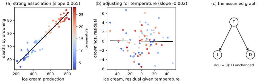
See also All of Statistics 16.1 for the potential-outcome version of the same warning, and Section 4.7.3 for seeing against doing.
36.2 Causal formalism
pp. 1187–1194 To make "intervene" precise and to encode causal knowledge as assumptions we need a model class that says more than a probability distribution does. The running example has four variables: smoking \(A\), lung cancer \(Y\), health consciousness \(H\) and a genetic predisposition \(G\).
36.2.1 Structural causal models
pp. 1187–1188, (36.1)–(36.8) Any joint distribution can be factorised in many orders, as in (36.1)–(36.4), and the orders carry the same information. A structural causal model (SCM) instead assigns each variable from its causes and independent exogenous noise, \[ G\leftarrow f_G(\xi_0),\quad H\leftarrow f_H(\xi_1),\quad A\leftarrow f_A(H,\xi_2),\quad Y\leftarrow f_Y(G,H,A,\xi_3) \tag{36.5--36.8} \] with the \(\xi_j\) independent. Sampling the noise and evaluating the assignments in order draws from \(P^{\mathrm{obs}}(G,H,A,Y)=P(G)P(H)P(A\given H)P(Y\given A,H,G)\), so an SCM implies a probabilistic model, but not conversely: the assignments are mechanisms, assumed invariant, and an intervention is an edit of one assignment. Setting smoking to zero replaces the third line by \(A\leftarrow0\), written \(\do(A=0)\). Because the order of the lines is load-bearing, an SCM cannot be rearranged by Bayes' rule without changing what it says about interventions (compare Section 4.7.2). SCMs do not capture every kind of causality (laws based on conservation or equilibrium, such as the ideal gas law, do not map to assignments), and the chapter confines itself to them.
36.2.2 Causal DAGs
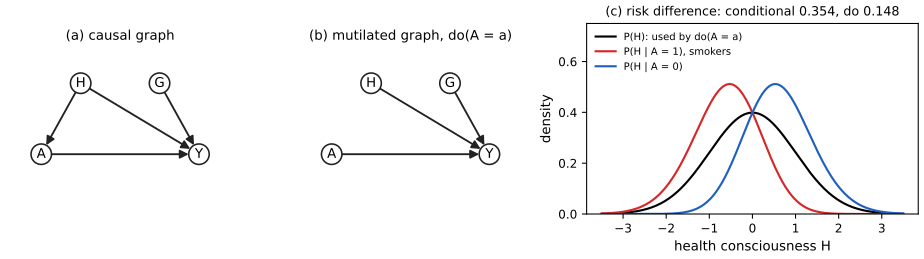
pp. 1188–1190, (36.9)–(36.11), Figure 36.2 Drawing an arrow from each right-hand-side variable to the left-hand side of each assignment gives the causal DAG of Figure 36.2(a). It implies the same conditional independences as a Bayesian network (d-separation, Section 4.2.4.1): a fork \(X\leftarrow Y\to Z\) gives \(X\indep Z\given Y\), and a collider \(X\to Y\leftarrow Z\) makes \(X\) and \(Z\) dependent given \(Y\), even if they are independent marginally. What the causal DAG adds is the meaning of intervention: graph surgery deletes every arrow into the intervened variable (Figure 36.2(b)) and then conditions on its value. The average treatment effect is \[ \ATE=\E[Y\given\do(A=1)]-\E[Y\given\do(A=0)]. \tag{36.9} \] Two variables can be associated through a directed path (smoking causes cancer), or through a backdoor path that starts with an arrow into \(A\) (\(A\leftarrow H\to Y\)). Even in a world with no effect of smoking, the backdoor path makes smoking and cancer associated, which is why association and causation differ. In the example, conditioning on \(A=a\) and intervening differ in a single factor: \[ P(Y,H,G\given A=a)=P(Y\given H,G,A=a)P(G)\,P(H\given A=a),\qquad P(Y,H,G\given\do(A=a))=P(Y\given H,G,A=a)P(G)\,P(H). \tag{36.10--36.11} \] Smokers are less health conscious than average, so \(P(H\given A=1)\) puts more mass on low \(H\) than \(P(H)\) does; the intervention instead keeps the population composition fixed.
Filling the gap 36.1: graph surgery equals the intervened SCM; (36.10) and (36.11) pp. 1189–1190
Proof
Take a Markovian SCM, \(V_i\leftarrow f_i(\pa_i,\xi_i)\) with independent noises. Then \(P(v)=\prod_iP(v_i\given\pa_i)\) with \(P(v_i\given\pa_i)=\Pr(f_i(\pa_i,\xi_i)=v_i)\), since given the parents the only randomness in \(V_i\) is \(\xi_i\), independent of the other noises. The SCM edited by \(A\leftarrow a\) is again a Markovian SCM, with the mechanism of \(A\) replaced by the constant \(a\) and all others unchanged, so its distribution is \(\prod_{i\ne A}P(v_i\given\pa_i)\) evaluated at \(A=a\): the factor \(P(a\given\pa_A)\) is deleted and \(a\) is substituted elsewhere. This is the truncated factorisation; it is what "delete the arrows into \(A\) and condition on \(A=a\)" computes, because in the surgically altered graph \(A\) is a root with the point-mass distribution at \(a\), and the CPDs of all other nodes are untouched.
For the graph of Figure 36.2, \(P(g,h,a,y)=P(g)P(h)P(a\given h)P(y\given g,h,a)\), so deleting the factor \(P(a\given h)\) gives \(P(g,h,y\given\do(A=a))=P(g)P(h)P(y\given g,h,a)\), which is (36.11). Conditioning on \(A=a\) instead keeps the factor and divides by \(P(a)\): \(P(g,h,y\given a)=P(g)P(h)P(a\given h)P(y\given g,h,a)/P(a)=P(g)P(h\given a)P(y\given g,h,a)\) by Bayes' rule, which is (36.10) (here \(G\indep A\)). The two differ exactly in the weight on \(H\): \(P(h\given a)\) against \(P(h)\).
Numbers. Let \(G\sim\mathrm{Bern}(0.3)\), \(H\sim\N(0,1)\), \(A=\Ind[\xi<-1.2H]\) with \(\xi\sim\N(0,1)\) (so \(P(A=1\given h)=\Phi(-1.2h)\)), and \(Y\sim\mathrm{Bern}(\sigma(-1.5+0.8A-0.9H+G))\). By quadrature over \(H\), the conditional risk difference \(P(Y{=}1\given A{=}1)-P(Y{=}1\given A{=}0)\) is \(0.354\), while the interventional one, \(\ATE\), is \(0.148\); smokers are enriched in low \(H\), which independently raises the risk, so more than half of the association is confounding. Simulating three million units from the SCM, with and without the edit of the \(A\) line, gives the same numbers (Figure 36.2(c)). In a discrete version of the same model I also confirmed (36.11) by enumeration. ∎
See also Result 4.13 (the truncated factorisation for a three-variable SCM) and All of Statistics Chapter 17 for d-separation.
36.2.3 Identification
pp. 1190–1192, (36.12) Many SCMs generate the same observed distribution, however large the sample. If a binary common cause \(U\) of treatment and outcome is unobserved, the data cannot say whether \(A\) has a strong effect, or none and \(U\) alone produces the association (Gap 36.2 builds both models). A causal estimand is identified under a set of assumptions, an identification strategy, if the assumptions leave only one value compatible with the observed distribution; the usual proof is by construction: write the estimand with no \(\do\) in it, a statistical estimand. In the running example, under the SCM above, \[ \ATE\overset{(*)}{=}\tau^{\mathrm{ATE}}\triangleq\E\bigl[\E[Y\given H,A=1]-\E[Y\given H,A=0]\bigr] \tag{36.12} \] (a special case of Theorem 2 below, with \(H\) the confounder; \(G\) need not be adjusted for because it affects only \(Y\)). Assumptions range from fully parametric (the cancer probability is additive on the logit scale in \(A,G,H\)), to monotonicity (smoking never lowers anyone's cancer risk), to purely structural statements of which variable affects which, as in a causal DAG. Non-parametric assumptions are minimal and are the plausible ones; some useful assumptions cannot be drawn in a graph (additive confounding in Section 36.5.1, parallel trends in 36.6) but are still weaker than a full parametric model.
Filling the gap 36.2: non-identifiability, and why every identifying assumption has untestable content pp. 1190–1192
Proof
(i) Two SCMs, one observed law. Let \(U\sim\mathrm{Bern}(\tfrac12)\), \(P(A=1\given U=u)=0.2+0.6u\), and in model 1 let \(P(Y=1\given A,U)=0.2+0.6U\) (no effect of \(A\)). The observed joint of \((A,Y)\) has \(P(A=1)=\tfrac12\) and \(P(Y=1\given A=a)=0.2+0.6P(U=1\given A=a)=0.68\) for \(a=1\) and \(0.32\) for \(a=0\). In model 2 there is no \(U\); \(A\sim\mathrm{Bern}(\tfrac12)\) and \(P(Y=1\given A=a)\) is set to the same two numbers. The two observed joints coincide, but \(\ATE=0\) in model 1 and \(0.68-0.32=0.36\) in model 2. Hence no estimator, however much data it sees, can learn the ATE from \((A,Y)\) alone, and the same holds for the whole distribution \(P(Y\given\do(A=1))\).
(ii) The width-one bounds. For binary \(A\) and \(Y\) without assumptions, \(\E[Y\given\do(A=1)]\in[P(Y=1,A=1),\,P(Y=1,A=1)+P(A=0)]\) (the unobserved outcomes of the untreated may be all 0 or all 1), and similarly for \(A=0\), so the ATE lies in an interval of width exactly 1 (Exercise 16.3 of All of Statistics works this out). Every value in the interval is generated by some SCM with the observed law.
(iii) Identifying assumptions cannot be fully checked. Suppose a class \(\mathcal M_0\) of SCMs is the set allowed by an identification strategy, so that on \(\mathcal M_0\) the ATE is a function \(\phi(P^{\mathrm{obs}})\). Take a model \(m\in\mathcal M_0\) with a non-degenerate law. By (ii), there is an SCM \(m'\), with the same observed law, whose ATE differs from that of \(m\). If \(m'\) were in \(\mathcal M_0\), then \(\mathrm{ATE}(m')=\phi(P^{\mathrm{obs}})=\mathrm{ATE}(m)\), a contradiction; so \(m'\notin\mathcal M_0\). The data from \(m\) therefore cannot distinguish \(m\), where the assumptions hold, from \(m'\), where they fail. This is the precise form of the book's statement that identification assumptions have unobservable implications: the assumptions may also have testable parts (overlap and instrument relevance can be read off the data), but never only testable parts. ∎
See also All of Statistics, gap 16.1 (what the data can never tell, in terms of response types).
36.2.4 Counterfactuals and the causal hierarchy
pp. 1192–1194, (36.13)–(36.15) SCMs support three kinds of query. Observational: statements about associations in the population. Interventional: statements about the population under a different assignment, \(P(Y\given\do(A=a))\); these only involve the marginal law of each potential outcome. Counterfactual: statements about individuals, "would Alice have developed cancer had she not smoked?", which need the joint law of her outcomes in different worlds. In the SCM, the potential outcome of unit \(i\) runs its noise through the intervened SCM, \[ Y_i(a)\triangleq f_Y(G_i,H_i,a,\xi_{3,i}). \tag{36.13} \] By Gap 36.1 the law of \(Y(a)\) is \(P(Y\given\do(A=a))\), and since the unedited SCM is the edited SCM at the realised \(A_i\), \(Y_i=Y_i(A_i)\) (consistency). Writing a query with potential outcomes does not make it counterfactual: the ATE is \(\E[Y(1)-Y(0)]\) (36.14), which only needs the two marginals, while a query that conditions on one potential outcome, such as \(\E[Y_i(0)\given Y_i(1)=1,A_i=1]\) (36.15), needs the dependence of \(Y(0)\) and \(Y(1)\) within individuals, which no data can show, since each unit reveals one of them. That is why counterfactual queries require assumptions on the functional form of the SCM, and interventional ones often only on the graph (Result 4.14 gives two couplings with identical interventional laws and different counterfactual answers). Potential outcomes and graphs are mathematically equivalent ways of stating the same assumptions: potential outcomes map directly to mechanistic intuition ("would I have smoked if I were more health conscious?"), graphs to many-variable structure.
36.3 Randomized control trials
pp. 1194–1195, (36.16)–(36.17), Figure 36.3 The simplest causal setting has no common cause of \(A\) and \(Y\). A randomised trial enforces this by design: assignment depends on nothing about the units, so \(A\) has no parents, graph surgery changes nothing, and \(P(Y\given\do(A=a))=P(Y\given A=a)\); the book remarks that the surgery definition is chosen to make this true, as any sensible formalisation of causality should. The ATE is then the parameter \(\tau^{\mathrm{RCT}}=\E[Y\given A=1]-\E[Y\given A=0]\) of the observed law, estimated by the difference of group means \[ \hat\tau^{\mathrm{RCT}}=\frac1{n_A}\sum_{i:A_i=1}Y_i-\frac1{n-n_A}\sum_{i:A_i=0}Y_i. \tag{36.17} \] Randomised trials are the gold standard because the triangle graph's no-unobserved-confounding assumption is true by design, but they can be infeasible (cost, regulation, outcomes observed decades later) and unrepresentative (trial participants may be younger and poorer than the patients who will take the drug). The estimator's unbiasedness, its variance \(\sigma_1^2/n_1+\sigma_0^2/n_0\), the Wald confidence interval, and the finite-population version are proved in Theorem 16.3 and Filling the gap 16.3 of All of Statistics; in a simulation of 2000 trials of 200 units with unequal variances, the 95 percent Neyman interval covered the ATE 94.6 percent of the time. Footnote 1 of the book points to more efficient trial estimators that adjust for covariates (Fisher, Lin, Bloniarz et al.); those are the estimators of Section 36.4.2 with \(g\equiv\tfrac12\) known.
36.4 Confounder adjustment
pp. 1195–1208 Now the data are observational, but we observe the common causes \(X\) of \(A\) and \(Y\) (Figure 36.3). The ATE is also called the average causal effect.
36.4.1 Causal estimand, statistical estimand, and identification
pp. 1195–1198, Theorem 2, (36.18)–(36.24), Definition 1 Confounders are common causes. Horseback riding in childhood and adult health are associated, but both are influenced by wealth \(X\): the riders are wealthier, so they are healthier even if riding has no benefit. The identification result needs two assumptions.
Theorem 2 (adjustment with no unobserved confounders) p. 1196, (36.19)
Observe \((A,Y,X)\sim P\). Suppose (1) confounders observed: the data follow the structure of Figure 36.3, so that \(X\) contains all common causes of \(A\) and \(Y\) and no variable in \(X\) is caused by \(A\) or \(Y\); (2) overlap: \(0<P(A=1\given X=x)<1\) for all \(x\). Then \(\ATE=\tau\), where \[ \tau=\E\bigl[\E[Y\given A=1,X]\bigr]-\E\bigl[\E[Y\given A=0,X]\bigr]=\E\bigl[Q(1,X)-Q(0,X)\bigr]. \tag{36.19} \]
Filling the gap 36.3: proof of Theorem 2 in the structural model, and the decomposition of the naive contrast pp. 1196–1197, (36.20)–(36.24)
Proof
Setting. Assumption (1) says: \(X\leftarrow f_X(\xi_X)\), \(A\leftarrow f_A(X,\xi_A)\), \(Y\leftarrow f_Y(A,X,\xi_Y)\) with \((\xi_X,\xi_A,\xi_Y)\) independent (\(X\) may be a vector of several variables with their own causes; only its non-descendance of \(A\) matters). Fix \(a\in\{0,1\}\).
Step 1 (what \(\do\) does). In the edited SCM, \(A\leftarrow a\), the mechanisms of \(X\) and \(Y\) are unchanged. So \(X\) has its original law, \(P(X\given\do(A=a))=P(X)\) (it is a non-descendant of \(A\)), and given \(X=x\) the outcome is \(f_Y(a,x,\xi_Y)\) with \(\xi_Y\) independent of \(X\). Hence \(\E[Y\given\do(A=a),X=x]=\E[f_Y(a,x,\xi_Y)]\), and by the tower property (36.21) \[ \E[Y\given\do(A=a)]=\E_X\bigl[\E[f_Y(a,X,\xi_Y)]\bigr]. \] Step 2 (what observation does). In the unedited SCM, on the event \(\{A=a,X=x\}\) the outcome is \(f_Y(a,x,\xi_Y)\), and \(\xi_Y\) is independent of \((\xi_X,\xi_A)\) and hence of \((X,A)\), which are functions of \((\xi_X,\xi_A)\). So \(\E[Y\given A=a,X=x]=\E[f_Y(a,x,\xi_Y)]\) for every \(x\) with \(P(A=a\given X=x)>0\). This is (36.22): the conditional law of \(Y\) given \((A,X)\) is the same in the original and the mutilated graph, because the only mechanism that changed is that of \(A\).
Step 3 (overlap). The right side of Step 2 must hold for \(P_X\)-almost every \(x\); the conditional expectation \(Q(a,x)\) is only determined where \(P(A=a\given X=x)>0\). With overlap, \(Q(1,x),Q(0,x)\) are defined for almost every \(x\), and \(\E[Y\given\do(A=a)]=\E[Q(a,X)]\). Subtracting gives (36.19). ∎
The naive contrast. By the tower property over \(X\), \(\E[Y\given A=a]=\int Q(a,x)P(x\given A=a)\,\d x\), so \[ \E[Y\given A=1]-\E[Y\given A=0]=\int Q(1,x)P(x\given A=1)\d x-\int Q(0,x)P(x\given A=0)\d x, \tag{36.24} \] whereas \(\tau\) integrates both against the same \(P(x)\) (36.23). The naive contrast equals \(\tau\) plus a selection term \(\int Q(1,x)[P(x\given A{=}1)-P(x)]\d x-\int Q(0,x)[P(x\given A{=}0)-P(x)]\d x\). For a linear outcome \(Q(a,x)=\beta_0+\tau a+\beta^\T x\) it equals \(\tau+\beta^\T\bigl(\E[X\given A=1]-\E[X\given A=0]\bigr)\): the bias is the effect of the covariates on \(Y\) times the imbalance of the covariates between the arms. On a discrete example (three covariate values, propensities 0.2, 0.5, 0.8) the naive contrast is 1.114 and \(\tau=1.150\), and (36.24) holds exactly. The proof is the same as Filling the gap 16.6 of All of Statistics written in graph language.
Definition 1 (overlap) p. 1197
\(P\) on \((A,X)\) satisfies overlap if \(0<P(A=1\given x)<1\) for all \(x\), and strict overlap if \(\epsilon<P(A=1\given x)<1-\epsilon\) for some \(\epsilon>0\).
pp. 1197–1198 Overlap says every unit could have received either treatment. Without it, an estimand cannot be identified without extra assumptions: if a drug was only ever given to men, nothing in the data informs \(E[Y\given A=1,X=\text{female}]\). With many covariates, combinations of traits can predict treatment almost perfectly even if no single trait does (men over 70 with BMI above 25 are rarely given the drug), and strict overlap then forces the confounders to be balanced almost as in a trial.
Filling the gap 36.4: why overlap is necessary, and how the variance of every estimator depends on it pp. 1197–1198, 1206
Proof
(i) Necessity. Let \(P(A=1\given X=x_0)=0\) on a set \(S\) of covariate values with \(P(X\in S)>0\). The observed law fixes \(Q(0,x)\) on \(S\) but places no restriction on \(Q(1,x)\), \(x\in S\): replacing \(Q(1,\cdot)\) by \(Q(1,\cdot)+h(\cdot)\mathbf 1_S\) leaves the law of \((X,A,Y)\) unchanged, while the ATE moves by \(\E[h(X)\mathbf 1_S]\), arbitrary. So the ATE is not a function of the observed law. On a discrete example (propensity 0 at one covariate value of mass 0.3) adding 5 to the unobserved \(Q(1,x_0)\) moves the ATE by 1.5 and changes nothing observable. The ATT of Section 36.4.5.3 is not affected (Gap 36.11).
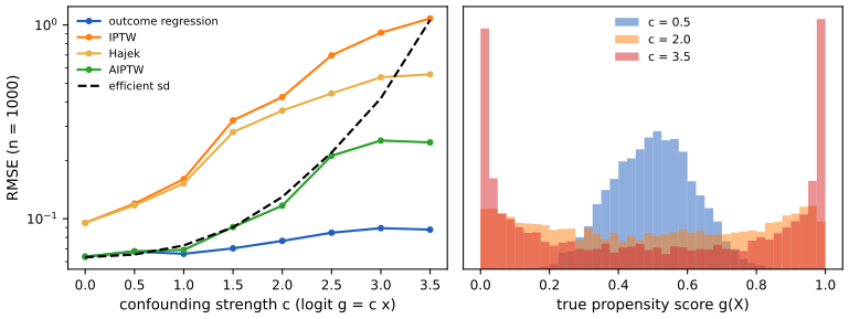
(ii) The variance depends on \(1/g\). Let \(\sigma_a^2(x)=\var(Y\given A=a,X=x)\) and \(\tau(x)=Q(1,x)-Q(0,x)\). The influence curve of Section 36.4.2.3 is \(\varphi=\tau(X)-\tau+A\varepsilon/g(X)-(1-A)\varepsilon/(1-g(X))\), where \(\varepsilon=Y-Q(A,X)\). Given \((A,X)\), \(\varepsilon\) has mean zero, so the cross terms vanish and \[ \E[\varphi^2]=\E\bigl[(\tau(X)-\tau)^2\bigr]+\E\Bigl[\frac{\sigma_1^2(X)}{g(X)}+\frac{\sigma_0^2(X)}{1-g(X)}\Bigr], \] because \(\E[A\varepsilon^2/g^2\given X]=\sigma_1^2/g\) and \(\E[(1-A)\varepsilon^2/(1-g)^2\given X]=\sigma_0^2/(1-g)\). This is the asymptotic variance of the best possible estimator (Gap 36.7), and it grows without bound as \(g\) approaches 0 or 1 on a non-negligible set: with homoskedastic noise it is \(\sigma^2\E[1/(g(1-g))]\) plus the heterogeneity term. For \(X\sim\N(0,1)\) and \(\logit g=cX\) one has \(1/(g(1-g))=2+e^{cX}+e^{-cX}\), hence \(\E[1/(g(1-g))]=2+2e^{c^2/2}\): 5.3 for \(c=1\), 47.5 for \(c=2.5\), 4.0 for \(c=0\) (confirmed by quadrature and simulation). Figure x36.2 shows the root mean square error of each estimator following this trend. The IPTW estimator has the extra problem that its own variance can be infinite (Gap 36.5).
(iii) Trimming changes the estimand. Dropping units with \(\hat g\notin[\epsilon,1-\epsilon]\) estimates the effect on the subpopulation \(\{\epsilon\le g\le1-\epsilon\}\), which equals the ATE only if the effect does not vary with \(g\) across the dropped and kept units. ∎
36.4.2 ATE estimation with observed confounders
pp. 1198–1203 Under the conditions of Theorem 2 the ATE equals the statistical estimand \(\tau\), and these estimation strategies are collectively called backdoor adjustment (the name comes from Section 36.8). Since confounders affect both treatment and outcome, one can model their influence on the outcome, on the treatment, or both.
36.4.2.1 Outcome model adjustment
pp. 1198–1199, (36.25)–(36.26) Define the conditional expected outcome \(Q(a,x)=\E[Y\given A=a,X=x]\) (36.25). Then \(\tau=\E[Q(1,X)-Q(0,X)]\), suggesting g-computation: fit \(\hat Q\) and average the predicted contrast over the empirical distribution of \(X\), \[ \hat\tau^{Q}=\frac1n\sum_i\hat Q(1,x_i)-\hat Q(0,x_i). \tag{36.26} \] \(Q\) is the minimiser over all square-integrable functions of \(\E[(Y-f(A,X))^2]\) (the mean minimises squared error: for any \(f\), \(\E[(Y-f)^2\given A,X]=\var(Y\given A,X)+(Q-f)^2\)), so fitting by least squares with a flexible model estimates it. For a unit that was treated, \(\hat Q(0,x_i)\) is a guess for the unseen counterfactual. If \(Q(A,X)=\beta_0+\beta_AA+\beta_X^\T X\) is linear, then \(Q(1,X)-Q(0,X)=\beta_A\) and \(\tau=\beta_A\): "fit a linear regression and report the coefficient of the treatment", a common way of estimating the association, is the special case of (36.26) in which the linear model is correct (I confirmed that my g-computation equals the least squares coefficient, and that both agree with statsmodels).
36.4.2.2 Propensity score adjustment
pp. 1199–1200, Definition 3, (36.27)–(36.29) The confounding effect can also be seen as the difference between \(P(X\given A=1)\) and \(P(X\given A=0)\). Reweighting the units so that the covariates have the same distribution in both arms removes it. The key quantity is the propensity score \(g(x)=P(A=1\given X=x)\) (Definition 3). Since \(A\) is binary, \[ \tau=\E\Bigl[\frac{YA}{g(X)}-\frac{Y(1-A)}{1-g(X)}\Bigr], \tag{36.27} \] which suggests the inverse probability of treatment weighted (IPTW) estimator and its self-normalised Hajek version, with \(\hat g\) fitted by predicting \(A\) from \(X\) (cross-entropy and squared error are proper scoring rules, so the minimiser is \(P(A=1\given X)\)): \[ \hat\tau^{\mathrm{IPTW}}=\frac1n\sum_i\frac{Y_iA_i}{\hat g(X_i)}-\frac{Y_i(1-A_i)}{1-\hat g(X_i)},\qquad \hat\tau^{h\text{-}\mathrm{IPTW}}=\frac{\sum_iY_iA_i/\hat g(X_i)}{\sum_iA_i/\hat g(X_i)}-\frac{\sum_iY_i(1-A_i)/(1-\hat g(X_i))}{\sum_i(1-A_i)/(1-\hat g(X_i))}. \tag{36.28--36.29} \] The estimator upweights treated units who were unlikely to be treated: they look like the untreated population, so their outcomes say what treatment would do to a typical untreated unit. It is asymptotically valid but unstable when estimated propensities are close to 0 or 1; the Hajek version helps somewhat, clipping weights is a common heuristic, and Khan and Ugander (2021) discuss improvements.
Filling the gap 36.5: proof of (36.27); what makes IPTW unstable and what the Hajek version fixes pp. 1199–1200
Proof
(i) The identity. \(\E[YA\given X]=\E[Y\given A=1,X]P(A=1\given X)=Q(1,X)g(X)\) (the term with \(A=0\) vanishes), so \(\E[YA/g(X)\given X]=Q(1,X)\), and likewise \(\E[Y(1-A)/(1-g)\given X]=Q(0,X)\). Averaging over \(X\) gives (36.27) from (36.19). This is an identity between two functionals of the observed law and uses no causal assumption; only overlap is needed so the divisions are defined. On the discrete example it holds exactly.
(ii) Consistency and variance. With the true \(g\), \(\hat\tau^{\mathrm{IPTW}}\) is a mean of iid terms, hence unbiased and root-\(n\) consistent when its summands have finite variance. The second moment of the treated term is \(\E[Y^2A/g^2]=\E[(\sigma_1^2+Q(1,X)^2)/g(X)]\), which is infinite when \(\E[1/g(X)]=\infty\) and \(Q(1,\cdot)\) is bounded away from 0 there. Example: \(X\sim\mathrm{Unif}(0,1)\), \(g(x)=x/2\), \(Q(1,x)=1\): \(\E[1/g]=\int_0^1(2/x)\d x=\infty\), so \(\hat\tau^{\mathrm{IPTW}}\) has infinite variance and no central limit theorem at the \(\sqrt n\) rate (strict overlap rules this out). This is the extreme version of the instability the book warns about.
(iii) The Hajek estimator. Write the treated half as \(\sum_iw_iY_i/\sum_iw_i\) with \(w_i=A_i/\hat g(X_i)\): it is a weighted average of the treated outcomes with weights summing to one, so it always lies between the smallest and largest treated outcome, whereas the IPTW estimate can leave that range. Consistency: by the law of large numbers \(\frac1n\sum w_iY_i\to\E[YA/g]=\E[Q(1,X)]\) and \(\frac1n\sum w_i\to\E[A/g]=1\), so the ratio converges to \(\E[Q(1,X)]\) by Slutsky's lemma. It is location equivariant: adding a constant \(c\) to every \(Y\) changes each weighted mean by \(c\) and the difference by 0, while \(\hat\tau^{\mathrm{IPTW}}\) changes by \(c\,(\frac1n\sum A_i/\hat g_i-\frac1n\sum(1-A_i)/(1-\hat g_i))\), which is \(0\) only in expectation. The Hajek version cannot remove strata where treatment is truly rare, or fix an overfitted \(\hat g\), so extreme weights can persist. ∎
See also All of Statistics, gap 16.8 (inverse probability weighting and its stratified estimate).
36.4.2.3 Double machine learning
pp. 1200–1202, (36.30)–(36.39) Each of the two strategies above is a two step procedure: fit a nuisance model, then plug it in. The quality of \(\hat\tau\) then depends on the quality of \(\hat Q\) or \(\hat g\), which may be complex functions that need many samples, so the naive estimators of the one-dimensional \(\tau\) can converge slowly. The augmented inverse probability of treatment weighted estimator (AIPTW) combines them: \[ \hat\tau^{\mathrm{AIPTW}}=\frac1n\sum_i\hat Q(1,X_i)-\hat Q(0,X_i)+A_i\frac{Y_i-\hat Q(1,X_i)}{\hat g(X_i)}-(1-A_i)\frac{Y_i-\hat Q(0,X_i)}{1-\hat g(X_i)}. \tag{36.30} \] It is the outcome-adjustment estimator plus a weighted-residual correction, and a member of the class of semiparametrically efficient or double machine learning estimators (Chernozhukov et al., 2017). With the influence curve \[ \phi(X_i,A_i,Y_i;Q,g,\tau)=Q(1,X_i)-Q(0,X_i)+A_i\frac{Y_i-Q(1,X_i)}{g(X_i)}-(1-A_i)\frac{Y_i-Q(0,X_i)}{1-g(X_i)}-\tau \tag{36.31} \] one has \(\hat\tau^{\mathrm{AIPTW}}-\tau=\frac1n\sum_i\phi(\cdot;\hat Q,\hat g,\tau)\). If \(Q,g\) were known, the central limit theorem would give \(\sqrt n(\hat\tau^{\mathrm{ideal}}-\tau)\to\N(0,\E[\phi(\cdot;Q,g,\tau)^2])\) (36.32). The naive outcome estimator, in contrast, needs \(\sqrt n\,\|\hat Q-Q\|_{L^2}\to0\): a root-\(n\) rate for \(Q\) itself. The book splits the error of \(\hat\tau^{\mathrm{AIPTW}}\) into three terms, (36.33)–(36.36): the ideal term, an empirical-process term for reusing the data, and a nuisance misestimation term, whose key property is that the errors of \(Q\) and \(g\) multiply. In the book's words the AIPTW is also doubly robust, non-parametrically efficient and asymptotically normal under a weak condition on the product of errors; Gaps 36.6 to 36.8 prove each of these properties and correct two misprints in the statement of the condition.
Filling the gap 36.6: the error decomposition, the exact bias formula, double robustness and the product rate pp. 1201–1202, (36.33)–(36.39)
Proof
Let \(Z=(X,A,Y)\) and \(\eta=(Q,g)\). Write \(\hat\phi=\phi(\cdot;\hat\eta,\tau)\), \(\phi_0=\phi(\cdot;\eta,\tau)\), \(P\) for the expectation over a fresh \(Z\) (with \(\hat\eta\) held fixed) and \(P_n\) for the sample mean.
(i) Decomposition. \(\hat\tau^{\mathrm{AIPTW}}-\tau=P_n\hat\phi=P_n\phi_0+(P_n-P)(\hat\phi-\phi_0)+P(\hat\phi-\phi_0)\), using \(P\phi_0=0\) (which holds by (36.19) and the tower property: \(\E[A(Y-Q(1,X))/g\given X]=0\)). Multiplying by \(\sqrt n\) gives the three terms of (36.34)–(36.36). The first is asymptotically \(\N(0,\E\phi_0^2)\) by the central limit theorem; the second is the empirical-process term (Gap 36.8); the third is the nuisance bias \(\sqrt n\,P(\hat\phi-\phi_0)\).
(ii) The exact bias. For fixed \(\hat Q,\hat g\), conditioning on \(X\) and using \(\E[A(Y-\hat Q_1)\given X]=g(Q_1-\hat Q_1)\) with \(Q_a=Q(a,X)\), \[ P\hat\phi=\E\Bigl[\hat Q_1-\hat Q_0+\frac{g(Q_1-\hat Q_1)}{\hat g}-\frac{(1-g)(Q_0-\hat Q_0)}{1-\hat g}\Bigr]-\tau. \] Subtract \(\tau=\E[Q_1-Q_0]\): the treated terms combine to \(\hat Q_1-Q_1+g(Q_1-\hat Q_1)/\hat g=(\hat Q_1-Q_1)(1-g/\hat g)=(\hat Q_1-Q_1)(\hat g-g)/\hat g\), and the control terms to \(-(\hat Q_0-Q_0)+(1-g)(\hat Q_0-Q_0)/(1-\hat g)=(\hat Q_0-Q_0)(\hat g-g)/(1-\hat g)\). Therefore \[ P(\hat\phi-\phi_0)=\E\Bigl[\frac{\hat g(X)-g(X)}{\hat g(X)}\bigl(\hat Q(1,X)-Q(1,X)\bigr)+\frac{\hat g(X)-g(X)}{1-\hat g(X)}\bigl(\hat Q(0,X)-Q(0,X)\bigr)\Bigr]. \] This is the book's (36.37)–(36.38) except that the denominators are \(\hat g\) and \(1-\hat g\), not \(g\) and \(1-g\) (with \(g\) the formula is wrong whenever \(\hat g\ne g\): on a discrete example with exact enumeration the right side is 0.306, the printed version \(-0.073\)). Both terms are products of an error in \(g\) and an error in \(Q\).
(iii) Double robustness. If \(\hat Q=Q\) (any \(\hat g\)) or \(\hat g=g\) (any \(\hat Q\)), every product vanishes, so \(P\hat\phi=0\) and \(\hat\tau\) is consistent as soon as \((P_n-P)\hat\phi\to0\): one correct nuisance suffices. Exact enumeration on three covariate values confirms this (correct \(Q\), wrong \(g\): unbiased; wrong \(Q\), correct \(g\): unbiased; both wrong: bias 0.306). The outcome estimator \(\hat\tau^Q\) is unbiased only if \(\hat Q=Q\) and IPTW only if \(\hat g=g\): the augmentation term corrects the first-order error of each.
(iv) The product rate. Assume strict overlap for the fit, \(\epsilon\le\hat g\le1-\epsilon\). By the Cauchy–Schwarz inequality, \[ \sqrt n\,|P(\hat\phi-\phi_0)|\le\frac{\sqrt n}{\epsilon}\,\|\hat g-g\|_{L^2}\bigl(\|\hat Q(1,\cdot)-Q(1,\cdot)\|_{L^2}+\|\hat Q(0,\cdot)-Q(0,\cdot)\|_{L^2}\bigr). \] So the third term vanishes if \(\sqrt n\,\|\hat g-g\|_2\max_a\|\hat Q(a,\cdot)-Q(a,\cdot)\|_2\to0\), that is, if the product of the two root mean square errors is \(o(n^{-1/2})\); each decreasing like \(o(n^{-1/4})\) suffices, which nonparametric learners can often attain. (The text says "the product of the misestimation errors is \(o(\sqrt n)\)", which is a slip: the displayed condition is \(\sqrt n\) times the product tends to 0. The weak condition printed before (36.39), \(\sqrt n\,\E(\hat Q-Q)^2\E(\hat g-g)^2\to0\), omits the square roots; with the square of the \(L^2\) norms it would allow, for example, errors of order \(n^{-1/8}\) each, for which the product \(n^{-1/4}\) times \(\sqrt n\) diverges.) By contrast \(\hat\tau^Q\) has nuisance bias \(P(\hat Q_1-\hat Q_0-Q_1+Q_0)\), first order in \(\|\hat Q-Q\|\), and \(\hat\tau^{\mathrm{IPTW}}\) has a bias first order in \(\|\hat g-g\|\): they need \(n^{-1/2}\) rates.
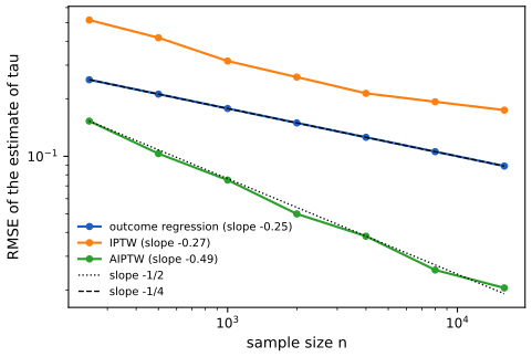
Simulation. I perturbed the true nuisances by \(n^{-1/4}\) times fixed smooth functions and recorded the root mean square error of three estimators over sample sizes from 250 to 16 000 (Figure x36.1): outcome regression, slope \(-0.25\); IPTW, \(-0.27\); AIPTW, \(-0.49\), the parametric rate. ∎
Filling the gap 36.7: \(\phi\) is the efficient influence curve, so \(\mathrm E[\phi^2]\) is the best possible variance p. 1202; footnote 6
Proof
The book states that AIPTW is non-parametrically efficient and omits the general theory (footnote 6). Here is the derivation for the ATE. Let \(\psi(P)=\E_P[Q_P(1,X)-Q_P(0,X)]=\int(\E_P[Y\given A=1,x]-\E_P[Y\given A=0,x])\,\d P(x)\) on the non-parametric model (all laws with overlap and finite variance). Take a smooth one-dimensional path \(P_\varepsilon\) with score \(s=s_X(x)+s_A(a\given x)+s_Y(y\given a,x)\), where each part has conditional mean zero given its conditioning variables. Then \[ \frac{\d}{\d\varepsilon}\psi(P_\varepsilon)\Big|_0=\E\bigl[(\tau(X)-\tau)s_X(X)\bigr]+\E\bigl[\partial_\varepsilon Q_\varepsilon(1,X)-\partial_\varepsilon Q_\varepsilon(0,X)\bigr]. \] The first term comes from differentiating \(\d P_\varepsilon(x)\) (subtracting \(\tau\) is free because \(\E s_X=0\)). For the second, \(\partial_\varepsilon Q_\varepsilon(a,x)=\E[(Y-Q(a,x))s_Y(Y\given a,x)\given A=a,X=x]\), so \(\E_X[\partial_\varepsilon Q(1,X)]=\E\bigl[\tfrac{A}{g(X)}(Y-Q(1,X))s_Y\bigr]\) (divide by \(P(A=1\given X)\), then multiply back by \(A\)). Because \(\E[Y-Q(A,X)\given A,X]=0\), the same expression with the full score \(s\) in place of \(s_Y\) is unchanged (the parts \(s_X(X)\) and \(s_A(A\given X)\) are functions of \((A,X)\) and multiply a conditionally mean-zero factor). Collecting terms, \[ \frac{\d}{\d\varepsilon}\psi(P_\varepsilon)\Big|_0=\E[\phi_0(Z)\,s(Z)],\qquad\phi_0=\tau(X)-\tau+\frac{A(Y-Q(1,X))}{g(X)}-\frac{(1-A)(Y-Q(0,X))}{1-g(X)}, \] which is (36.31). A function with this property that lies in the tangent space is the efficient influence function; in a non-parametric model the tangent space is all of \(L^2_0(P)\), so \(\phi_0\) is the only influence function, and the convolution (Hajek–Le Cam) theorem (van der Vaart, 1998, Theorem 25.20), which I quote, says that every regular estimator has asymptotic variance at least \(\E[\phi_0^2]\). An estimator with \(\hat\tau-\tau=P_n\phi_0+o_P(n^{-1/2})\), as AIPTW has under the conditions of Gap 36.6, attains it. By Gap 36.4 this variance is \(\E[(\tau(X)-\tau)^2]+\E[\sigma_1^2/g+\sigma_0^2/(1-g)]\); a simulation of three million units from a three-valued covariate model gives \(\E[\phi^2]=7.785\) against the closed form \(7.798\). ∎
36.4.2.4 Cross fitting
p. 1202 The empirical-process term (36.35) is the price of using the same data to fit \(Q,g\) and to average. For many model classes it is negligible, but not always. A simple remedy is sample splitting, fitting on one half and averaging on the other, at the cost of using only half the data for each task. Cross fitting with \(K\) folds improves on it: for each fold \(j\), fit \(\hat Q_{-j},\hat g_{-j}\) on the other \(K-1\) folds and evaluate \(\hat Q_{-j}(a_i,x_i),\hat g_{-j}(x_i)\) for the points \(i\) in fold \(j\); then plug the out-of-fold predictions into (36.30). The code is aiptw_crossfit.
Filling the gap 36.8: why cross fitting makes the empirical-process term vanish; the variance estimator pp. 1202–1203, (36.40)
Proof
(i) The empirical-process term. Let fold \(j\) have \(n_j\) points and let \(\hat\eta_{-j}\) be fitted on the other folds. Define the contribution of the fold, \(R_j=n^{-1/2}\sum_{i\in\text{fold }j}\bigl[\hat\phi_j(Z_i)-\phi_0(Z_i)-P(\hat\phi_j-\phi_0)\bigr]\) with \(\hat\phi_j=\phi(\cdot;\hat\eta_{-j},\tau)\). Conditional on the training folds, the \(Z_i\) in fold \(j\) are iid and independent of \(\hat\eta_{-j}\), so the summands are iid with mean zero, and \[ \E[R_j^2\given\hat\eta_{-j}]=\frac{n_j}n\,\var\bigl(\hat\phi_j(Z)-\phi_0(Z)\given\hat\eta_{-j}\bigr)\le\frac{n_j}{n}\,\|\hat\phi_j-\phi_0\|_{L^2(P)}^2. \] If the nuisance estimators are \(L^2\)-consistent and strict overlap holds, then \(\|\hat\phi_j-\phi_0\|_{L^2}\to0\) (each term of \(\phi\) is a Lipschitz function of \(\hat Q,\hat g\) when \(\hat g\) is bounded away from 0 and 1), so \(R_j\to0\) in probability by Chebyshev's inequality, for each of the \(K\) folds. The sum \(\sum_jR_j\) is the second term of the decomposition, and it vanishes without any complexity condition on the model class (a Donsker condition would be needed without splitting). The price is \(K\) model fits and models trained on \(\tfrac{K-1}{K}n\) points. Cross fitting has the same asymptotic guarantee as the idealised estimator.
(ii) The variance estimator (36.40). The estimator \(\hat V=\frac1n\sum_i\phi(Z_i;\hat\eta,\hat\tau)^2\) satisfies \(\bigl|\hat V^{1/2}-(P_n\phi_0^2)^{1/2}\bigr|\le\bigl(P_n(\hat\phi-\phi_0)^2\bigr)^{1/2}\) by the triangle inequality in \(\mathbb R^n\) (the Minkowski inequality), and the right side tends to 0 in probability when \(\|\hat\phi-\phi_0\|_{L^2}\to0\) and \(\hat\tau\to\tau\) (take expectations over folds as above and use Markov's inequality), while \(P_n\phi_0^2\to\E\phi_0^2\) by the law of large numbers. So \(\hat V\to\E[\phi_0^2]\), the interval \(\hat\tau\pm1.96\sqrt{\hat V/n}\) has asymptotic coverage 95 percent, and no bootstrap with nuisance refitting is needed. In 400 simulated samples of size 800 (5 folds, quadratic outcome and propensity models, the setting of Figure 36.3 with both models flexible) the interval covered the true ATE 96.3 percent of the time. ∎
36.4.3 Uncertainty quantification
p. 1203, (36.40) A point estimate needs a measure of uncertainty. The asymptotic normality (36.39) gives intervals from the limiting variance \(\E[\phi(Z;Q,g,\tau)^2]\); the plug-in estimate (36.40), \(\hat V[\hat\tau]=\frac1n\sum_i\phi(Z_i;\hat Q,\hat g,\hat\tau)^2\), gives a 95 percent interval \(\hat\tau\pm1.96\sqrt{\hat V/n}\) (Gap 36.8). The alternative is the bootstrap, which must refit the nuisance functions for every replicate and can be too expensive.
36.4.4 Matching
pp. 1203–1204, (36.41)–(36.42) Matching pairs each treated unit with controls that have the same (or close) confounders and compares the outcomes. For a discrete \(X\) with \(\mathcal A_x\) the treated and \(\mathcal C_x\) the untreated units at \(X=x\), \[ \hat\tau^{\mathrm{matching}}=\sum_x\hat P(x)\Bigl(\frac1{|\mathcal A_x|}\sum_{i\in\mathcal A_x}Y_i-\frac1{|\mathcal C_x|}\sum_{j\in\mathcal C_x}Y_j\Bigr). \tag{36.41} \] Writing \(Y_i=Q(A_i,X_i)+\xi_i\) with \(\E[\xi_i\given A_i,X_i]=0\) gives (36.42): the matching estimator is \(\sum_x\hat P(x)(Q(1,x)-Q(0,x))\) plus a difference of averages of mean-zero noise, which tends to 0 as the cell counts grow. Two remarks of the book: the argument has nothing to do with identification (matching estimates the observational \(\tau\); whether \(\tau\) is causal is decided by Theorem 2), and matching is a particular choice of outcome model, \(\hat Q(1,x)=\) the cell mean. When any function \(\varphi(X)\) satisfies \(A\indep X\given\varphi(X)\), adjusting for \(\varphi(X)\) alone suffices, and the most popular choice is the propensity score itself (propensity score matching).
Filling the gap 36.9: matching is a saturated outcome regression; balancing scores pp. 1203–1204
Proof
(i) Matching equals g-computation with cell means. Let the outcome model be saturated in \(x\): \(Q(a,x)\) is a separate parameter for every cell \((a,x)\). Least squares fits it by the cell mean, \(\hat Q(1,x)=|\mathcal A_x|^{-1}\sum_{\mathcal A_x}Y_i\), and then \(\hat\tau^Q\) in (36.26), which weights cells by the empirical frequency \(\hat P(x)\), is exactly (36.41). This was confirmed numerically (4000 units, three covariate values). If a stratum lacks treated or control units the estimator is undefined, which is the finite-sample face of the overlap condition; my code drops such strata and renormalises.
(ii) Balancing scores. Suppose \(g(X)=P(A=1\given X)\) and \(\varphi(X)\) is any function with \(g(X)=P(A=1\given\varphi(X))\) (the propensity score, or anything that determines it). Then \(P(A=1\given X,\varphi(X))=P(A=1\given X)=g(X)\), which is a function of \(\varphi(X)\), so \(P(A=1\given X,\varphi)=P(A=1\given\varphi)\), that is, \(A\indep X\given\varphi(X)\). Consequently, within a stratum of \(\varphi\), the covariate distribution is the same in the treated and control arms: the propensity score balances the covariates (checked on a five-valued covariate with two propensity values: \(P(X\given A=1,g)=P(X\given A=0,g)=P(X\given g)\)).
(iii) Adjusting for \(\varphi\) alone gives the same \(\tau\). Let \(\tilde Q(a,\varphi)=\E[Y\given A=a,\varphi(X)]\). By the tower property and the balance in (ii), \(\tilde Q(a,\varphi)=\E[Q(a,X)\given A=a,\varphi]=\E[Q(a,X)\given\varphi]\), the last step using \(X\indep A\given\varphi\). Hence \(\E[\tilde Q(1,\varphi)-\tilde Q(0,\varphi)]=\E[Q(1,X)-Q(0,X)]=\tau\). The same follows from (36.27), in which \(\tau\) depends on \(X\) only through \(g(X)\). Reducing \(X\) to a coarser \(\varphi\) with the same propensity cannot change \(\tau\); checked exactly on the five-valued example. This is why propensity score matching is a valid estimator of \(\tau\), and why, once more, validity as a causal estimate depends only on Theorem 2. ∎
36.4.5 Practical considerations and procedures
36.4.5.1 What to adjust for
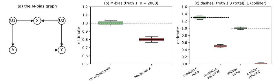
pp. 1204–1206, Figure 36.4 With the full graph the rule is clear: adjust for the common causes (in particular for the parents of \(A\), Gap 36.10), and Section 36.8 generalises this. Without the graph, it is tempting to condition on everything observed, and that can hurt. A mediator \(M\), on a directed path from \(A\) to \(Y\), carries part of the effect; conditioning on it removes that part, and since the mediated effect may run opposite to the direct one, the estimate can shrink, grow or flip sign. A collider \(C\), caused by both \(A\) and \(Y\), induces a dependence between them when conditioned on. Limiting adjustment to pre-treatment variables avoids both, but can still go wrong: if a covariate \(X\) is a collider of two unobserved causes \(U_1\to A\) and \(U_2\to Y\) (the M-bias graph of Figure 36.4), where \(A\) and \(Y\) are not confounded, conditioning on \(X\) opens the path \(A\leftarrow U_1\to X\leftarrow U_2\to Y\) and creates bias even though \(X\) precedes the treatment. VanderWeele and Shpitser (2011) refine the heuristic to "condition on pre-treatment variables that are causes of treatment, outcome or both", which avoids M-bias but needs knowledge of causal ancestry. Variance can be reduced by dropping variables that are known to affect only the treatment (instruments, Section 36.5). Finally, if no observed set blocks all backdoor paths, every adjusted estimate is biased, and the bias does not necessarily fall as more variables are added: adjusting for an instrument amplifies it (bias amplification, or z-bias, Gap 36.17).
Filling the gap 36.10: adjusting for the parents of \(A\) is valid; closed forms for M-bias, a mediator and a collider pp. 1204–1206
Proof
(i) Parents suffice. Let \(X=\pa(A)\) be observed. A backdoor path from \(A\) to \(Y\) starts \(A\leftarrow P\cdots\) with \(P\in\pa(A)\). On that path the node \(P\) has an outgoing arrow towards \(A\), so it is not a collider; conditioning on \(P\) blocks the path. Hence \(\pa(A)\) blocks every backdoor path, and contains no descendant of \(A\) in a DAG, so it satisfies the backdoor criterion of Section 36.8, and Theorem 2 applies with \(X=\pa(A)\). (In the SCM of Theorem 2 this is the statement that \(\xi_A\) is independent of the noise that drives \(Y\) once \(X=\pa(A)\) is fixed.)
(ii) M-bias in the linear Gaussian model. Let \(U_1,U_2\) be standard normal and \(A=U_1+\epsilon_A\), \(X=U_1+U_2+\epsilon_X\), \(Y=\tau A+U_2+\epsilon_Y\), all noises standard normal and independent. Then \(\var A=2\), \(\var X=3\), \(\cov(A,X)=1\), \(\cov(A,Y)=2\tau\), \(\cov(X,Y)=\tau+1\). Without adjustment the coefficient of \(A\) is \(\cov(A,Y)/\var A=\tau\): there is no confounding. Regressing \(Y\) on \((A,X)\) the coefficient of \(A\) is \[ \frac{\var X\,\cov(A,Y)-\cov(A,X)\cov(X,Y)}{\var A\,\var X-\cov(A,X)^2}=\frac{6\tau-(\tau+1)}{5}=\tau-\tfrac15 . \] Adjusting for \(X\) biases the effect by \(-0.2\): 0.8 for \(\tau=1\) (simulation of four million units: 0.7997, Figure 36.4(b)).
(iii) Mediator. Let \(M=0.8A+\epsilon\), \(Y=0.5A+M+\epsilon'\) with a randomised standard normal \(A\). The total effect is \(0.5+0.8\cdot1=1.3\), which is what the regression of \(Y\) on \(A\) estimates (no confounding); regressing on \((A,M)\) gives the direct effect 0.5. If the mediated path were negative (\(M\leftarrow 0.8A\), \(Y\leftarrow-1.5M+0.5A\)), the total effect would be \(0.5-1.2=-0.7\) while the coefficient adjusted for \(M\) is \(+0.5\): the sign flips, because the adjusted coefficient is always the direct edge.
(iv) Collider. Let \(A\sim\N(0,1)\), \(Y=A+\epsilon\), \(C=A+Y+\nu\) with standard normal noises. Then \(\var C=6\), \(\cov(A,C)=2\), \(\cov(Y,C)=3\), \(\cov(A,Y)=1\) and the coefficient of \(A\) in the regression of \(Y\) on \((A,C)\) is \((6\cdot1-2\cdot3)/(1\cdot6-2^2)=0\): the true effect 1 is estimated as exactly zero (Figure 36.4(c)). ∎
36.4.5.2 Overlap
p. 1206 With infinite data any amount of overlap suffices, but near failures hurt in practice: the asymptotic variance \(\E[\phi^2]/n\) contains terms proportional to \(1/g(X)\) and \(1/(1-g(X))\) and balloons when units have \(g\approx0\) or \(1\) (Gap 36.4). A simple check, which the analysis needs anyway, is to fit \(\hat g\) and look at its values; if some are extreme, the simplest resolution is to drop those units, which changes the estimand to the average effect over the subpopulation with overlap, and whether that answers the real-world question has to be argued from domain knowledge. Figure x36.2 shows the effect: with confounding strength \(c\) (so \(\logit g=cX\)) the efficient standard deviation grows like \(\sqrt{2+2e^{c^2/2}}\), and the weighting estimators follow it while outcome regression, whose model here is correct, does not.
36.4.5.3 Choice of estimand and the average treatment effect on the treated
pp. 1206–1207, (36.43)–(36.47) The goal is often qualitative (the sign, whether the effect is large), and an estimand that answers it more easily may be preferable to the ATE. The average treatment effect on the treated is \[ \ATT\triangleq\E_{X\given A=1}\bigl[\E[Y\given X,\do(A=1)]-\E[Y\given X,\do(A=0)]\bigr]. \tag{36.43} \] It is useful when many units are very unlikely to receive treatment but the treated had a reasonable probability of being controls, for example controls sampled from the population and the treated self-selected from a subpopulation: the ATT omits the units with no similar treated unit. Under the structure of Figure 36.3 and the weaker overlap condition \(P(A=1\given X=x)<1\) for all \(x\), \(\ATT=\tau^{\mathrm{ATT}}=\E_{X\given A=1}\bigl[\E[Y\given A=1,X]-\E[Y\given A=0,X]\bigr]\) (36.44). Estimators translate by averaging over the treated only; a double machine learning estimator that also uses the untreated units is \[ \hat\tau^{\mathrm{ATT\text{-}AIPTW}}=\frac1n\sum_i\frac{A_i}{P(A=1)}\bigl(Y_i-\hat Q(0,X_i)\bigr)-\frac{(1-A_i)\hat g(X_i)}{P(A=1)(1-\hat g(X_i))}\bigl(Y_i-\hat Q(0,X_i)\bigr), \tag{36.45} \] with variance estimated from the influence curve \(\phi^{\mathrm{ATT}}\) of (36.46)–(36.47). It needs no model for \(Q(1,X)\), a real advantage when the treated are rare.
Filling the gap 36.11: identification of the ATT with weaker overlap, and double robustness of (36.45) pp. 1206–1207
Proof
(i) Identification. The population averaged over is that of the treated, \(P(X\given A=1)\), which has density ratio \(P(x\given A{=}1)/P(x)=g(x)/P(A{=}1)\) with respect to \(P(X)\); so the only values of \(x\) that matter have \(g(x)>0\). By Step 1 of Gap 36.3, \(\E[Y\given X=x,\do(A=a)]=f(a,x)\triangleq\E f_Y(a,x,\xi_Y)\) and \(f(a,x)=Q(a,x)\) whenever \(P(A=a\given X=x)>0\). For \(a=1\) this holds on \(\{g>0\}\), which has probability one under \(P(X\given A=1)\); for \(a=0\) one needs \(g(x)<1\) there, which is the stated overlap condition. Hence the ATT equals (36.44). Nothing is required about \(Q(1,x)\) or \(Q(0,x)\) where \(g(x)=0\) (units never treated) or about \(Q(0,x)\) at \(g(x)=1\) (but \(g=1\) must have probability zero among the treated). On the discrete example with \(g=0\) at one covariate value (mass 0.3), where the ATE is not identified (Gap 36.4), the ATT is \(1.366\) and the estimator (36.45) applied to 1.5 million units gives 1.366.
(ii) Double robustness of (36.45). Let \(p_A=P(A=1)\) and write \(\hat Q_0=\hat Q(0,X)\), \(\hat g=\hat g(X)\). Conditioning on \(X\), \(\E[A(Y-\hat Q_0)\given X]=g(Q_1-\hat Q_0)\) and \(\E[(1-A)(Y-\hat Q_0)\given X]=(1-g)(Q_0-\hat Q_0)\), so \[ p_A\E[\hat\tau^{\mathrm{ATT\text{-}AIPTW}}]=\E\Bigl[g(Q_1-\hat Q_0)-\frac{(1-g)\hat g}{1-\hat g}(Q_0-\hat Q_0)\Bigr]. \] If \(\hat Q_0=Q_0\) the second term vanishes and the right side is \(\E[g(Q_1-Q_0)]=p_A\tau^{\mathrm{ATT}}\). If \(\hat g=g\) the bracket is \(g(Q_1-\hat Q_0)-g(Q_0-\hat Q_0)=g(Q_1-Q_0)\) again. So it is consistent if either \(Q(0,\cdot)\) or \(g\) is. The ATT is generally different from the ATE when the effect varies with \(X\) (on the example, the ATE is 1.30 and the ATT 1.366). ∎
36.4.6 Summary and practical advice
pp. 1207–1208, Figure 36.3 (estimation) All estimators follow the same recipe: fit \(\hat Q(a,x)\) and/or \(\hat g(x)\); compute \(\hat Q(0,x_i),\hat Q(1,x_i),\hat g(x_i)\); combine into an estimate. No estimator is uniformly best; the double machine learning estimators have appealing asymptotics and a recipe for uncertainty without bootstrap, but can underperform their naive counterparts in practice (Kang and Schafer, 2007). Causal problems have fewer guardrails than prediction: the estimand is a functional of a different distribution from the observed one, so a train-test split cannot validate it. The sanity checks are to (i) compute several estimators (regression, weighting, doubly robust) with comparably flexible models, and see whether they agree; (ii) look at the distribution of the (cross-fitted) \(\hat g(x_i)\), even if the final estimator is outcome regression; (iii) report a standard error, bootstrapping the whole procedure or using the influence-curve variance, remembering that a huge variance often signals overlap trouble and a tiny one deserves suspicion; and (iv) assess the no-unobserved-confounding assumption itself (Section 36.7), whose violation can dominate estimation error.
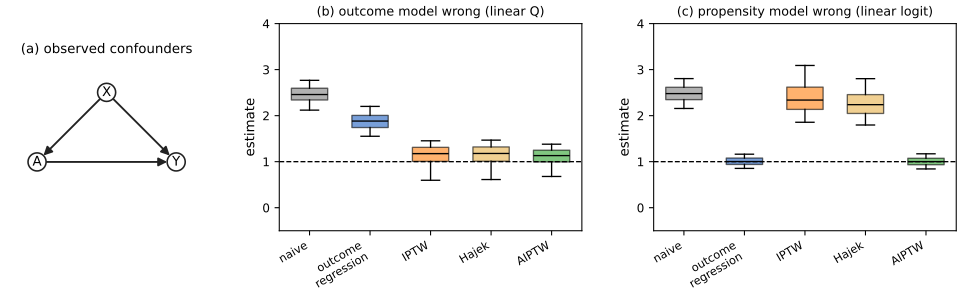
Figure 36.3 is a simulation of the whole story. One normal confounder \(X\) drives treatment through \(\logit g(x)=x+0.6(x^2-1)\) and the outcome through \(Y=A+x+1.2(x^2-1)+\epsilon\) (true ATE 1, standard normal noise). The table gives the mean and standard deviation of each estimator over 500 samples of size 500, fitting the outcome and propensity models either with a quadratic term (right) or without (wrong):
| estimator | both models right | outcome model wrong | propensity model wrong | both wrong |
|---|---|---|---|---|
| naive difference in means | 2.47 (0.21) | 2.46 (0.20) | 2.48 (0.20) | 2.45 (0.19) |
| outcome regression | 1.00 (0.09) | 1.88 (0.20) | 1.01 (0.10) | 1.87 (0.19) |
| IPTW | 0.99 (1.92) | 1.07 (0.67) | 2.41 (0.51) | 2.36 (0.40) |
| Hajek | 1.09 (0.60) | 1.11 (0.43) | 2.28 (0.38) | 2.24 (0.32) |
| AIPTW | 1.00 (0.13) | 1.06 (0.50) | 1.00 (0.10) | 2.39 (0.42) |
The naive contrast is off by a factor 2.5; with one correct nuisance the AIPTW estimator is right (doubly robust), with both wrong it is as wrong as the others. The standard deviations of IPTW are large (1.92 in the first column, from a few very large weights), the point of Gap 36.5. The demonstration lets you change the confounding, the overlap and the misspecification.
36.5 Instrumental variable strategies
pp. 1208–1216, Figure 36.5 Adjustment needs every confounder observed. Sometimes an effect can still be identified when an unobserved confounder \(U\) affects both \(A\) and \(Y\), if there is an instrumental variable \(Z\): a variable that affects \(Y\) only through \(A\) (Figure 36.5). Informally, one finds the causal effect of \(Z\) on \(Y\), the causal effect of \(Z\) on \(A\), and combines them. For this to work, with observed covariates \(X\), the instrument must satisfy three conditions: (1) relevance, \(Z\nindep A\given X\); (2) unconfoundedness, every backdoor path between \(Z\) and \(Y\) is blocked by \(X\), even conditional on \(A\); (3) exclusion restriction, every directed path from \(Z\) to \(Y\) passes through \(A\). These are necessary but not sufficient: they must be supplemented by an assumption on the form of the process (historically, linearity; below, additive confounding or monotonicity). Instruments are common: the random assignment of a drug with non-compliance (relevance if assignment changes uptake; unconfoundedness by randomisation; exclusion plausible unless unassigned patients seek other treatment), or the judge fixed-effects design (the identity of the judge assigned to a criminal case, which is randomised, instruments the sentence). Relevance can be checked from the data; unconfoundedness is often satisfied by design; the exclusion restriction needs domain knowledge, since it fails if judges add unrecorded punishments.
36.5.1 Additive unobserved confounding
pp. 1210–1211, (36.48)–(36.55), Theorem 3 Assume the outcome mechanism is additive in the unobserved confounder, \[ Y\leftarrow f(A,X)+f_U(U), \tag{36.48} \] so everyone responds to treatment in the same way (no interaction of \(A\) with \(U\)). Then \(\E[Y\given X,\do(A=a)]-\E[Y\given X,\do(A=a')]=f(a,X)-f(a',X)\), and this contrast is the target.
Theorem 3 (additive confounding identification) pp. 1210–1211, (36.49)–(36.51)
If the instrumental variable assumptions and additive unobserved confounding hold, there is a function \(\tilde f(a,x)\) with \(\E[Y\given x,\do(A=a)]-\E[Y\given x,\do(A=a')]=\tilde f(a,x)-\tilde f(a',x)\) for all \(x,a,a'\), and \(\tilde f\) satisfies \[ \E[Y\given z,x]=\int\tilde f(a,x)\,p(a\given z,x)\,\d a. \tag{36.50} \] If \(g\) is the unique solution of \(\E[Y\given z,x]=\int g(a,x)p(a\given z,x)\d a\), then \(g=\tilde f\) and the effect is identified.
The point is that the left side and the kernel \(p(a\given z,x)\) of (36.51) are identified by the data, so \(\tilde f\) is identified implicitly as a solution; one fits models for \(\E[Y\given z,x]\) and \(p(a\given z,x)\) and solves the equation (see the references of the book for concrete methods, for example neural networks with a norm penalty to pick one solution). Relevance does not enter the proof; it enters through uniqueness.
Filling the gap 36.12: proof of Theorem 3, and when the integral equation has a unique solution pp. 1210–1211
Proof
(i) The causal contrast. In the SCM \(Y\leftarrow f(A,X)+f_U(U)\), the intervention \(\do(A=a)\) does not change the law of \((X,U)\) (neither is a descendant of \(A\)), so \(\E[Y\given X=x,\do(A=a)]=f(a,x)+\E[f_U(U)\given X=x]\). The second term does not depend on \(a\) and cancels in the contrast: \(f(a,x)-f(a',x)\), which also shows that additivity is what makes the second term cancel (with an \(A\)-\(U\) interaction it would not).
(ii) The observed identity. Instrument unconfoundedness gives \(U\indep Z\given X\) (the exclusion restriction is implied by the additive structure: \(Z\) does not appear in the outcome equation). Then \[ \E[Y\given Z,X]=\E[f(A,X)\given Z,X]+\E[f_U(U)\given Z,X]=\E[f(A,X)\given Z,X]+\E[f_U(U)\given X], \] and with \(\tilde f(a,x)=f(a,x)+\E[f_U(U)\given x]\) this is \(\E[\tilde f(A,X)\given Z,X]=\int\tilde f(a,X)p(a\given Z,X)\d a\), which is (36.50). Because \(\tilde f\) differs from \(f\) by a function of \(x\) alone, \(\tilde f(a,x)-\tilde f(a',x)=f(a,x)-f(a',x)\), the causal contrast. If a second function \(g\) solves (36.51) then \(g=\tilde f\) by the uniqueness assumption, so the contrast is identified from observables. (Without uniqueness, only the set of solutions is identified.)
(iii) Uniqueness is relevance and more. For fixed \(x\), (36.51) is a Fredholm integral equation of the first kind in \(a\mapsto g(a,x)\). If \(Z\) and \(A\) are discrete with \(K_A\) and \(K_Z\) values, it is the linear system \(\bm P\bm g=\bm m\) with \(P_{za}=p(a\given z)\) and \(m_z=\E[Y\given z]\). Its solution is unique iff \(\operatorname{rank}\bm P=K_A\), which requires \(K_Z\ge K_A\) (at least as many instrument values as treatment levels) and distinct rows. An irrelevant instrument has \(p(a\given z)\) not depending on \(z\), so all rows are equal, the rank is 1, and one only learns \(\sum_ag(a)p(a)\); a weak instrument has nearly equal rows, so \(\bm P\) is ill-conditioned and tiny errors in \(\hat{\bm m}\) or \(\hat{\bm P}\) become huge errors in \(\hat{\bm g}\). On a three-level example with \(P=\begin{pmatrix}0.6&0.3&0.1\\0.3&0.4&0.3\\0.1&0.3&0.6\end{pmatrix}\) and \(f=(0,1,3)\), solving the system with the observed \(\E[Y\given z]\) (including a constant confounding shift) recovers the contrasts \(f(1)-f(0)=1\), \(f(2)-f(1)=2\) exactly; with identical rows the rank is 1. For continuous \(A\), uniqueness is the completeness of \(p(a\given z)\) (\(\int h(a)p(a\given z)\d a=0\) for all \(z\) implies \(h=0\); Newey and Powell, 2003), a stronger condition than correlation and one that makes the estimation problem ill-posed. When \(f\) is linear in \(a\), (36.50) reduces to the single equation of Section 36.5.3. ∎
36.5.2 Instrument monotonicity and local average treatment effect
pp. 1212–1215, (36.56)–(36.82), Theorem 4 When both the instrument and treatment are binary, think of \(Z\) as assignment to treatment. The population has four types: compliers (take the treatment iff assigned), always takers, never takers and defiers (refuse iff assigned). The ATE cannot be identified, because always and never takers never respond to the instrument; the target is the effect among compliers, the local average treatment effect (complier average treatment effect), \[ \LATE=\E[Y\given\do(A=1),\text{complier}]-\E[Y\given\do(A=0),\text{complier}]. \tag{36.56} \] (The book writes LATE because CATE is already used for the conditional average treatment effect.) Identification needs monotonicity: assignment never lowers the probability of taking the treatment, \(P(\text{defier})=0\).
Theorem 4 p. 1212, (36.57)
Under the instrumental variable assumptions and monotonicity, \(\LATE=\tau^{\mathrm{LATE}}\) with \[ \tau^{\mathrm{LATE}}=\frac{\E\bigl[\E[Y\given X,Z=1]-\E[Y\given X,Z=0]\bigr]}{\E\bigl[P(A=1\given X,Z=1)-P(A=1\given X,Z=0)\bigr]}. \tag{36.57} \]
Filling the gap 36.13: the LATE proof, what monotonicity buys, and what fails without it pp. 1212–1213, (36.58)–(36.70)
Proof
The book's proof is complete; here it is in its simplest form, with \(X\) absent (with \(X\), apply the steps within strata of \(X\), average numerator and denominator over \(P(X)\), and note that (36.58) uses Theorem 2 with \(Z\) as the treatment, which is exactly what unconfoundedness of the instrument given \(X\) provides). Each unit has potential treatments \(A(1),A(0)\) and potential outcomes \(Y(a)\); the type is a function of \((A(0),A(1))\), and the instrument is independent of \((A(0),A(1),Y(0),Y(1))\) (unconfoundedness without covariates), with \(Y=Y(A)\) and exclusion (the potential outcome depends on \(Z\) only through \(A\)).
(i) The decomposition. \(\E[Y\given Z=1]-\E[Y\given Z=0]=\sum_{t}P(t)\bigl(\E[Y(A(1))\given t]-\E[Y(A(0))\given t]\bigr)\) over types \(t\), because the type distribution is the same in both instrument arms (\(Z\) is independent of the type; this is the book's statement that interventions on the instrument do not change the population composition). By type: compliers, \(A(1)=1,A(0)=0\): \(\E[Y(1)-Y(0)\given c]=\LATE\); always takers, \(A(1)=A(0)=1\), and never takers, \(A(1)=A(0)=0\): zero (they ignore the instrument; exclusion makes the outcome the same in both arms); defiers, \(A(1)=0,A(0)=1\): \(-\E[Y(1)-Y(0)\given d]\). With \(P(d)=0\): \[ \text{ITT}\triangleq\E[Y\given Z{=}1]-\E[Y\given Z{=}0]=P(c)\,\LATE. \] (ii) The first stage. \(P(A=1\given Z=1)=P(c)+P(a)+0\cdot P(n)+0\) and \(P(A=1\given Z=0)=P(a)\) (always takers and, absent defiers, nobody else), so \(P(A=1\given Z{=}1)-P(A=1\given Z{=}0)=P(c)\). Dividing, \(\LATE=\text{ITT}/\text{(first stage)}\), the Wald estimator's population version, which is (36.57) and (36.58). It requires \(P(c)>0\), that is, relevance.
(iii) Without monotonicity. Let \(\theta_c,\theta_d\) be the average effects among compliers and defiers. The same decomposition gives \(\text{ITT}=P(c)\theta_c-P(d)\theta_d\) and the first stage is \(P(c)-P(d)\), so the Wald ratio is \(\dfrac{P(c)\theta_c-P(d)\theta_d}{P(c)-P(d)}\), an effect-weighted difference in which defiers enter with a negative weight: it can lie outside the range of the effects and can have the wrong sign (with \(P(c)=0.5\), \(\theta_c=1\) and \(\theta_d=2\): \(P(d)=0.1\) gives 0.75, \(P(d)=0.2\) gives 0.33, \(P(d)=0.25\) gives \(0\)). Figure x36.3(a) shows the formula against a simulation of 400 000 units: the points follow it, and the as-treated contrast stays far off because always takers and never takers are different kinds of people.
(iv) Exclusion fails. If \(Z\) has a direct effect \(\rho\) on \(Y\), the ITT gains \(\rho\) and the Wald ratio becomes \(\LATE+\rho/P(c)\) (here \(1+0.3/0.5=1.6\), confirmed by simulation): a small violation is magnified by the inverse of the complier share.
(v) A misprint. Equations (36.59) and (36.69) write \(\E[Y\given\do(Z=1)]-\E[Y\given\do(Z=1)]\); the second term should be \(\do(Z=0)\). ∎
See also All of Statistics 16.1 for response types without an instrument; the compliance strata here are the four response types for the treatment.
36.5.2.1 Estimation
pp. 1213–1215, (36.71)–(36.82) A double machine learning estimator works with generic supervised learners. With the nuisances \(\mu(z,x)=\E[Y\given z,x]\), \(m(z,x)=P(A=1\given x,z)\), \(p(x)=P(Z=1\given x)\), define the scores \[ \phi_{Z\to Y}=\mu(1,X)-\mu(0,X)+\frac{Z(Y-\mu(1,X))}{p(X)}-\frac{(1-Z)(Y-\mu(0,X))}{1-p(X)},\qquad \phi_{Z\to A}\text{ the same with }(A,m), \tag{36.75--36.76} \] \(\phi=\phi_{Z\to Y}-\tau\,\phi_{Z\to A}\) (36.77), and let \(\hat\tau^{\mathrm{LATE}}\) solve \(\frac1n\sum_i\phi(X_i;\hat\mu,\hat m,\hat p,\hat\tau)=0\), that is, the ratio of the double machine learning estimates of the effect of \(Z\) on \(Y\) and on \(A\) (36.78). Fit \(\hat\mu\) (squared error), \(\hat m\) and \(\hat p\) (cross-entropy), with cross fitting. If the nuisance estimators are \(L^2\)-consistent and \(\|\hat p-p\|_2(\|\hat\mu-\mu\|_2+\|\hat m-m\|_2)=o(n^{-1/2})\), then \(\sqrt n(\hat\tau^{\mathrm{LATE}}-\tau^{\mathrm{LATE}})\to\N\bigl(0,\E[\phi^2]/\E[m(1,X)-m(0,X)]^2\bigr)\) (36.79), and the variance estimate (36.81) uses \(\hat\tau_{Z\to A}=\frac1n\sum\phi_{Z\to A}\). The variance estimate also needs all nuisances at rate \(n^{-1/4}\); it is unnecessary when \(p\) is known, as for a randomised instrument. (The text writes "\(o(\sqrt n)\)" in the product condition; as in Gap 36.6 it should be \(o(n^{-1/2})\).)
Filling the gap 36.14: the LATE estimator is a ratio of two AIPTW estimators; its influence curve and rate pp. 1214–1215, (36.77)–(36.82)
Proof
Apply the AIPTW theory of Gaps 36.6 and 36.7 with \(Z\) as the treatment and \(Y\), then \(A\), as the outcome: \(\frac1n\sum\phi_{Z\to Y}\) estimates \(\theta_Y=\E[\mu(1,X)-\mu(0,X)]\) and \(\frac1n\sum\phi_{Z\to A}\) estimates \(\theta_A=\E[m(1,X)-m(0,X)]\), each with the product-rate property in \((\hat p,\hat\mu)\) or \((\hat p,\hat m)\). The parameter is \(\tau=\theta_Y/\theta_A\). Solving \(P_n\hat\phi_{Z\to Y}-\hat\tau P_n\hat\phi_{Z\to A}=0\) gives exactly (36.78). Subtracting \(\tau\) times the second sum,
\[ \hat\tau-\tau=\frac{P_n\bigl(\hat\phi_{Z\to Y}-\tau\hat\phi_{Z\to A}\bigr)}{P_n\hat\phi_{Z\to A}}=\frac{P_n\hat\phi(\tau)}{P_n\hat\phi_{Z\to A}}. \]
The denominator converges to \(\theta_A=P(\text{complier})>0\) (relevance; the identity follows from Gap 36.13(ii)). The numerator is \(P_n\hat\phi\) for the score (36.77) at the true \(\tau\), whose expectation at the truth is zero (\(\theta_Y-\tau\theta_A=0\)). Exactly as in Gap 36.6, with the same product bias terms for \(\phi_{Z\to Y}\) and (times \(\tau\)) \(\phi_{Z\to A}\), it equals \(P_n\phi_0+o_P(n^{-1/2})\) under the stated product condition and cross fitting. By Slutsky, \(\sqrt n(\hat\tau-\tau)\to\N(0,\E\phi_0^2/\theta_A^2)\), which is (36.79). The delta method for the ratio \(\theta_Y/\theta_A\) gives the same influence function \((\phi_{Z\to Y}-\tau\phi_{Z\to A})/\theta_A\), the efficient one, and (36.81) estimates it by the plug-in. The factor \(1/\theta_A^2\) is why weak instruments are costly: halving the complier share quadruples the variance of the estimator. When \(Z\) is randomised, \(p\) is known, the product terms involving \(\hat p-p\) vanish, and the estimator is root-\(n\) consistent for arbitrary \(\hat\mu,\hat m\) (a consistent \(\hat\mu\) is not even needed); in the code, late_dml, 150 simulated samples of 2000 units with a confounded binary instrument centre at \(1.008\) (truth 1, standard deviation 0.089). The Wald estimator's delta-method standard error (influence function \(\psi_{\mathrm{ITT}}-\tau\psi_{\mathrm{FS}}\) over the first stage) agrees with the bootstrap (0.1443 against 0.1447). ∎
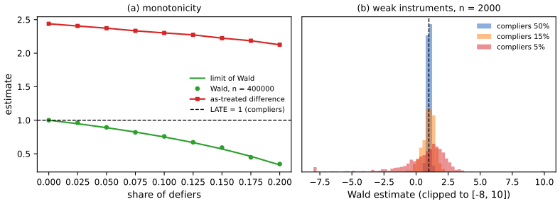
The IV demonstration lets you change the complier, always-taker and defier shares, the selection and the exclusion violation, and compares the as-treated contrast, the intention-to-treat effect and the Wald estimate.
36.5.3 Two stage least squares
pp. 1215–1216, (36.83)–(36.85) Commonly, the instrumental variable assumptions are supplemented by linear structural equations for \(A\) and \(Y\), \[ A\leftarrow\alpha_0+\alpha Z+\gamma_A^\T X+\xi^A,\qquad Y\leftarrow\beta_0+\beta A+\gamma_Y^\T X+\xi^Y \tag{36.83--36.84} \] (the book writes the covariate terms twice, \(\delta_AX+\gamma_AX\); one covariate coefficient vector per equation is what is meant). Substituting the first into the second gives \(Y\leftarrow\tilde\beta_0+\beta\alpha Z+\tilde\gamma^\T X+\tilde\xi\) (36.85): \(\beta\) is the coefficient of the instrument in the outcome equation divided by its coefficient in the treatment equation. Fitting both linear models and dividing the coefficients is two stage least squares (2SLS). The simplicity is seductive, but linearity is hard to satisfy and the consequences can be severe: misspecification together with weak relevance can make the standard errors far too small, so large "significant" estimates appear when the truth is a weak or null effect (the book cites Reiersol, Young, Andrews et al., Lal et al.).
Filling the gap 36.15: why 2SLS works, the ordinary least squares limit, and weak instruments pp. 1215–1216; Figure 36.5
Proof
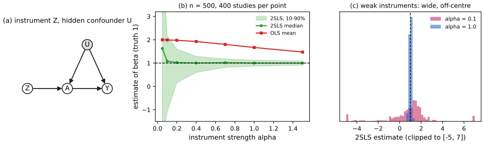
(i) Consistency. Take the model of Figure 36.5(b) with no covariates: \(U,Z\sim\N(0,1)\), \(A=\alpha Z+U+\eta\), \(Y=\beta A+2U+\epsilon\) with standard normal \(\eta,\epsilon\). Then \(\cov(Z,Y)=\beta\alpha\) (as \(Z\) is independent of \(U,\epsilon\)) and \(\cov(Z,A)=\alpha\), so \(\hat\beta^{2SLS}=\widehat{\cov}(Z,Y)/\widehat{\cov}(Z,A)\to\beta\) as long as \(\alpha\ne0\). (With one instrument and no covariates, the two-stage procedure of regressing \(Y\) on the fitted values \(\hat A=\hat\pi Z\) gives \(\hat\beta=\widehat\cov(\hat A,Y)/\widehat\var(\hat A)=\widehat\cov(Z,Y)/\widehat\cov(Z,A)\), and for a binary \(Z\) this is the Wald estimator exactly: both equalities were confirmed to machine precision.) Ordinary least squares converges instead to \[ \beta+\frac{\cov(A,2U+\epsilon)}{\var A}=\beta+\frac{2}{\alpha^2+2}, \] the confounded limit: 1.667 for \(\alpha=1\) (simulation: 1.661), and nearly \(\beta+1\) as \(\alpha\to0\).
(ii) Weak instruments. \(\hat\beta-\beta=\sum z_i(2u_i+\epsilon_i)/\sum z_iA_i\). The denominator has mean \(n\alpha\) and standard deviation of order \(\sqrt n\), so when \(\alpha\) is of the order \(n^{-1/2}\) it is often near 0 and the ratio is heavy-tailed: in the just-identified case the 2SLS estimator has no finite mean (Kinal, 1980, whose result I quote). With \(n=500\) and \(\alpha=0.05\) the 10–90 percent range of 400 simulated estimates is 6.9 wide (0.25 for \(\alpha=1\)), the median has moved from 1.00 to 1.53 towards the OLS limit 2.0, and Figure 36.5(c) shows the wide, off-centre distribution. The median bias towards OLS is the typical weak-instrument behaviour: the first-stage fit \(\hat A\) is dominated by the noise in \(A\) that is correlated with \(U\). Intervals computed as if the estimator were normal are then wrong, hence the book's warning. ∎
36.6 Difference in differences
pp. 1216–1219, (36.86)–(36.94), Theorem 5, Figure 36.6 Causes precede effects, and observing each unit at several times gives a further identification strategy. In the simplest panel data case there are two periods: in the first no unit is treated and we observe \(Y_{0i}\); then a subset (\(A_i=1\)) is treated and in the second period we observe \(Y_{1i}\). The goal is the average effect on the treated: the average difference between what we saw for the treated and what we would have seen had they not been treated. The strategy is called difference in differences (DiD). The motivating example is Card and Krueger's (1994) study of the minimum wage: New Jersey (\(A=1\)) raised its minimum wage on 1 April 1992, from 4.25 to 5.05 dollars, and Pennsylvania did not; fast-food restaurants in both states were surveyed in February and November 1992, \(Y_{ti}\) the number of full-time employees. The classical assumption is the structural equation \[ Y_{ti}\leftarrow W_i+S_t+\tau A_i\Ind(t=1)+\xi_{ti},\qquad\E[\xi_{ti}\given W_i,S_t,A_i]=0, \tag{36.86} \] where \(W_i\) is a unit effect constant over time (location, management) and \(S_t\) a time effect common to all units (the economy), both unobserved, and \(\tau\) is the target effect. Unit, time and treatment effects are additive: this is the parallel trends assumption, that without treatment the two groups would have moved in parallel. It gives \[ \tau=\E[Y_{1i}-Y_{0i}\given A=1]-\E[Y_{1i}-Y_{0i}\given A=0],\qquad\hat\tau=\frac1{n_A}\sum_{i:A_i=1}(Y_{1i}-Y_{0i})-\frac1{n-n_A}\sum_{i:A_i=0}(Y_{1i}-Y_{0i}). \tag{36.87--36.88} \] The root problem it solves is \(\E[W_i\given A=1]\ne\E[W_i\given A=0]\): New Jersey and Pennsylvania restaurants differ in unobserved ways that affect employment, so the levels cannot be compared; here, however, \(W_i\) need not cause treatment (unlike a confounder). The assumption can be too strong: if expensive chains (more common in New Jersey) are hit harder by a recession than cheap ones, trends differ even absent the policy. So the book states a version that requires parallel trends only after adjusting for covariates, with a non-parametric causal estimand: using the notation \(P_{A=1}(Y\given\do(A=a))\triangleq\int P(Y\given A=a,\text{parents of }Y)\,\d P(\text{parents of }Y\given A=1)\) (36.89)–(36.90) (the do operator with the covariate distribution of the treated), the estimand is \[ \ATT^{\mathrm{DiD}}=\E_{A=1}[Y_1-Y_0\given\do(A=1)]-\E_{A=1}[Y_1-Y_0\given\do(A=0)] \tag{36.91} \] and the identifying assumption is conditional parallel trends: \(\E_{A=1}[Y_1-Y_0\given X,\do(A=0)]=\E[Y_1-Y_0\given X,A=0]\) (36.92): had New Jersey not raised its wage, its McDonald's would have had the same expected change as Pennsylvania's McDonald's.
Theorem 5 (difference in differences identification) pp. 1218–1219, (36.93)
Observe \((A,Y_0,Y_1,X)\sim P\). Suppose (1) the data follow the graph of Figure 36.6 (the change \(Y_1-Y_0\) is influenced by \(A\), unobserved factors \(U\) and covariates \(X\)); (2) conditional parallel trends (36.92); (3) overlap: \(P(A=1)>0\) and \(P(A=1\given X=x)<1\) for all \(x\). Then \(\ATT^{\mathrm{DiD}}=\tau^{\mathrm{DiD}}\), where \[ \tau^{\mathrm{DiD}}=\E\Bigl[\E[Y_1-Y_0\given A=1,X]-\E[Y_1-Y_0\given A=0,X]\Bigm|A=1\Bigr]. \tag{36.93} \]
Filling the gap 36.16: the DiD identification in potential outcomes, the bias when trends depend on covariates, and estimation pp. 1216–1219
Proof
(i) The classical model. From (36.86), \(Y_{1i}-Y_{0i}=S_1-S_0+\tau A_i+\xi_{1i}-\xi_{0i}\); the unit effect \(W_i\) cancels, whatever its dependence on \(A_i\). Taking expectations in each arm, \(\E[\Delta Y\given A=a]=\E[S_1-S_0\given A=a]+\tau a\) (the noise terms have mean zero given \(A\)), and under parallel trends, \(\E[S_1-S_0\given A=1]=\E[S_1-S_0\given A=0]\), the difference of arms is \(\tau\), which is (36.87).
(ii) Theorem 5 in potential outcomes. Let \(Y_1(a)\) be the second-period outcome under treatment \(a\), with \(Y_0\) the first-period (untreated, no anticipation) outcome and \(Y_1=Y_1(A)\). The target is \(\ATT=\E[Y_1(1)-Y_1(0)\given A=1]\). Then \[ \ATT=\E[Y_1-Y_0\given A=1]-\E[Y_1(0)-Y_0\given A=1], \] the second term being the unobserved trend of the treated had they not been treated. Conditional parallel trends says \(\E[Y_1(0)-Y_0\given X,A=1]=\E[Y_1(0)-Y_0\given X,A=0]=\E[Y_1-Y_0\given X,A=0]\) (the last by consistency, since \(A=0\) units show \(Y_1(0)\)), defined on the support of \(X\) among the treated because \(P(A=0\given X)>0\) there (overlap). Averaging over \(P(X\given A=1)\) yields (36.93). This is the book's "unrolling of definitions": the first line of the proof is \(\E_{A=1}[Y_1-Y_0\given\do(A=1),X]=\E[Y_1-Y_0\given A=1,X]\) (consistency) and the second is the assumption (36.92).
(iii) Unconditional DiD can be biased. In the simulation of Figure 36.6, restaurants are cheap (0) or expensive (1); expensive chains are in the treated state with probability 0.7, cheap with 0.3, and the trend without treatment is \(-0.5\) for cheap and \(-1.5\) for expensive chains. Then \(\E[S\text{-trend}\given A=1]-\E[\cdot\given A=0]=(-1.5-(-0.5))(P(X{=}1\given A{=}1)-P(X{=}1\given A{=}0))=-1\cdot(0.7-0.3)=-0.4\), and the unadjusted estimator (36.88) has bias \(-0.40\) (simulation of three million units: \(-0.402\)), whereas (36.93) estimated by regression of the change on \(X\) in the control group has bias below 0.005. Parallel trends needs to hold conditional on the right covariates.
(iv) The estimation task is the ATT task. Put \(\tilde Y=Y_1-Y_0\). Then (36.93) is \(\E[\E[\tilde Y\given A=1,X]-\E[\tilde Y\given A=0,X]\given A=1]\), the ATT estimand of (36.44) with outcome \(\tilde Y\), so every estimator of Section 36.4.5.3 applies unchanged: outcome regression (fit \(\hat Q(0,x)\) on the controls and average \(\tilde Y_i-\hat Q(0,X_i)\) over the treated, my did_adjusted), the weighted estimator and the double machine learning estimator (36.45). The identification argument differs from the adjustment case, the estimation task does not. The classical estimator (36.88) also equals the coefficient of the interaction \(A_i\Ind(t=1)\) in the two-way least squares regression of \(Y\) on treated-arm, period and their interaction (checked to machine precision): the saturated \(2\times2\) model reproduces the four cell means.
(v) Credibility. Parallel trends is needed at the treatment date only, so it cannot be refuted by later divergences (administrative data show Pennsylvania's employment falling relative to New Jersey's between 1993 and 1996), but divergences make it less credible; a placebo analysis of earlier periods (Section 36.7.1) is the usual check. ∎
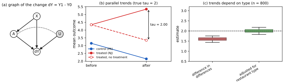
36.7 Credibility checks
pp. 1219–1228 After choosing an identification strategy and producing an estimate, the question is whether to believe it. That depends on the identification assumptions, the quality of the models and the sampling variability. The last two are familiar: assess models on held-out data and report confidence intervals. The assumptions come in two kinds. Some can be checked from the data (overlap, instrument relevance), and must be. Others cannot (no unobserved confounding, the exclusion restriction, conditional parallel trends: Gap 36.2); two supplementary analyses help to judge them.
36.7.1 Placebo checks
p. 1220 A placebo treatment is a variable known to have no effect on the outcome but expected to be confounded in the same way as the real treatment: to study a COVID vaccine one might use HPV vaccination, since health consciousness and fear of needles affect both. If the identification strategy is valid for the real treatment, it should be valid for the placebo and give \(\hat\tau\approx0\), or at least an interval containing 0; otherwise confounders are still lurking. A null outcome works the same way: an outcome the treatment cannot affect but that shares confounders with the real one (symptomatic COVID within 7 days of vaccination, when the biology says the vaccine cannot have acted yet), analysed with the same strategy. In a linear example with a hidden confounder \(U\) (treatment \(A=U+\eta\), outcome \(Y=U+\epsilon\), no true effect, \(\eta,\epsilon\) standard normal), a regression of \(Y\) on a placebo treatment \(A'=U+\eta'\) gives the coefficient \(\cov(A',Y)/\var(A')=1/2\), far from 0 with any reasonable sample, and flags the confounding that the same adjustment would leave in the real analysis. A passing placebo is evidence, not proof: the placebo's confounding may just differ from the real treatment's.
36.7.2 Sensitivity analysis to unobserved confounding
pp. 1221–1228, (36.96)–(36.106), Theorems 6–8, Figure 36.7 For the adjustment setting of Section 36.4, causal identification rests on "no unobserved confounding", which the data cannot test. A violation can explain the association entirely or partly, so we ask how strong a hidden confounder would have to be. Cornfield et al. (1959) showed for smoking and lung cancer that a hormone would have to raise the probability of smoking by at least a factor of nine to explain the association away, which is implausible for a hormone. To make such judgements routine one must define "strength of confounding" and translate it into bias.
Imbens' model. Imbens (2003) (after Rosenbaum and Rubin, 1983) posits a binary hidden confounder with \[ U_i\sim\mathrm{Bern}(\tfrac12),\quad A_i\given X_i,U_i\sim\mathrm{Bern}(\sigma(\gamma X_i+\alpha U_i)),\quad Y_i\given X_i,A_i,U_i\sim\N(\tau A_i+\beta X_i+\delta U_i,\sigma^2). \tag{36.96--36.98} \] Given plausible \(\alpha^*\) (influence of \(U\) on treatment) and \(\delta^*\) (on outcome), the other parameters can be estimated, giving \(\hat\tau(\alpha^*,\delta^*)\). The drawback is that it requires a parametric model of the whole data (logistic for the treatment, linear for the outcome), which rules out the neural networks and random forests that are state of the art for effect estimation.
Austen plots (Veitch and Zaveri, 2020) decouple the sensitivity analysis from the modelling of the observed data. The idea is to posit a simple, interpretable form for the influence of the hidden confounder, with no constraint on the observed-data models, and to formalise confounding strength with unitless parameters, comparable with the strength of the observed covariates. The plot shows the curve of all sensitivity parameters that would induce a given bias, moving the analyst's judgement from "what are plausible values of the parameters?" to "are parameters this extreme plausible?".
Setup. Data \((Y_i,A_i,X_i,U_i)\) are iid, \(U_i\) unobserved. If \(X\) contains all common causes then \(\ATE=\tau\) with \(\tau=\E[Q(1,X)-Q(0,X)]\) (36.99). With a hidden \(U\), \(\tau\) is not the ATE and the inference splits in two tasks: the statistical one (estimate \(\tau\) well, with any \(\hat Q,\hat g,\hat\tau\)) and the causal one (assess \(\mathrm{bias}\), the gap between \(\tau\) and the ATE, which concerns misidentification, not the statistical bias of the estimator). Imbens' functional form is \(\logit P(A=1\given x,u)=h(x)+\alpha u\) and \(\E[Y\given a,x,u]=l(a,x)+\delta u\) (36.100–36.101); eliminating \(u\) shows that \(U\) influences the outcome only through the propensity \(\tilde g(x,u)=P(A=1\given x,u)\) (Definition 36.7.1). So one can put a distribution on \(\tilde g\) directly, centred at the observed propensity score: \[ \tilde g(X,U)\given X\sim\mathrm{Beta}\Bigl(g(X)\bigl(\tfrac1\alpha-1\bigr),\,(1-g(X))\bigl(\tfrac1\alpha-1\bigr)\Bigr),\quad A\given X,U\sim\mathrm{Ber}(\tilde g(X,U)), \tag{36.103--36.104} \] \[ \E[Y\given A,X,U]=Q(A,X)+\delta\bigl(\logit\tilde g(X,U)-\E[\logit\tilde g(X,U)\given A,X]\bigr). \tag{36.105} \] For \(\alpha\) near 0, \(\tilde g\) is tightly concentrated at \(g(X)\) and \(U\) tells us little about treatment; for \(\alpha\) near 1 it piles up at 0 and 1 and \(U\) nearly determines treatment (Figure x36.4(b)). The model is built so that \(P(A=1\given X)=g(X)\) and \(\E[Y\given A,X]=Q(A,X)\): it imposes nothing on the observed data. The sensitivity parameters are \(\alpha\) and \(\delta\).
Theorem 6 pp. 1224–1225
Under the Austen model (36.105), an unobserved confounder with influence \(\alpha\) and \(\delta\) induces a bias of absolute size \[ |\mathrm{bias}|=\frac{|\delta|}{1/\alpha-1}\,\E\Bigl[\frac1{g(X)}+\frac1{1-g(X)}\Bigr]=|\delta|\,\frac{\alpha}{1-\alpha}\,\E\Bigl[\frac1{g(X)(1-g(X))}\Bigr]. \]
The bias is determined by the sensitivity parameters and the realised propensity score; more extreme propensity scores give more extreme bias for the same confounding. In particular, conditioning on a covariate that affects treatment but not the outcome (an instrument) increases any bias due to unobserved confounding: z-bias.
Filling the gap 36.17: the bias of the Austen model (Theorem 6), its sign, and z-bias pp. 1223–1225
Proof
Write \(k=1/\alpha-1\), \(a=g(X)k\), \(b=(1-g(X))k\) and \(L=\logit\tilde g\).
(i) The model reproduces the observed law. \(\tilde g\given X\sim\mathrm{Beta}(a,b)\) has mean \(a/(a+b)=g(X)\), so \(P(A=1\given X)=\E[\tilde g\given X]=g(X)\), and variance \(\dfrac{ab}{(a+b)^2(a+b+1)}=g(1-g)\alpha\) (since \(a+b+1=1/\alpha\)). In (36.105), \(\E[Y\given A,X]=\E[\E[Y\given A,X,U]\given A,X]=Q(A,X)\) because the correction \(L-\E[L\given A,X]\) has conditional mean zero.
(ii) Beta-Bernoulli conjugacy. Given \(X\), the prior of \(\tilde g\) is \(\mathrm{Beta}(a,b)\) and \(A\given\tilde g\sim\mathrm{Ber}(\tilde g)\), so the posterior of \(\tilde g\) given \(A=1\) is \(\mathrm{Beta}(a+1,b)\) and given \(A=0\) is \(\mathrm{Beta}(a,b+1)\). For \(u\sim\mathrm{Beta}(a',b')\), \(\E\log u=\psi(a')-\psi(a'+b')\) and \(\E\log(1-u)=\psi(b')-\psi(a'+b')\) with \(\psi\) the digamma function, so \(\E\,\logit u=\psi(a')-\psi(b')\). Hence \[ m_1\triangleq\E[L\given X,A=1]=\psi(a+1)-\psi(b),\qquad m_0\triangleq\E[L\given X,A=0]=\psi(a)-\psi(b+1), \] \[ m_1-m_0=[\psi(a+1)-\psi(a)]+[\psi(b+1)-\psi(b)]=\frac1a+\frac1b=\frac1k\Bigl(\frac1g+\frac1{1-g}\Bigr)=\frac{\alpha}{1-\alpha}\,\frac1{g(1-g)} \] by the recurrence \(\psi(x+1)-\psi(x)=1/x\) (verified by numerical quadrature of the two posterior means for several \((g,\alpha)\)).
(iii) The bias and its sign. By (36.105), \(\E[Y\given A=a',X,U]=Q(a',X)+\delta(L-m_{a'})\) for \(a'\in\{0,1\}\) (the unit's propensity \(L\) is the same under both treatments: \(U\) does not change). The model's ATE, using the identification from \((X,U)\), is \[ \ATE=\E\bigl[\E[Y\given A{=}1,X,U]-\E[Y\given A{=}0,X,U]\bigr]=\tau+\delta\,\E_X[m_0-m_1]=\tau-\delta\,\frac{\alpha}{1-\alpha}\E\Bigl[\frac1{g(1-g)}\Bigr], \] since the terms in \(L\) cancel in the difference. The magnitude of \(\ATE-\tau\) is the Theorem 6 bias. The sign: for \(\delta>0\), the hidden confounder raises both treatment probability and outcome, so the observed contrast overstates the effect and \(\ATE<\tau\); the book writes the bias with a plus sign but defines it as \(\ATE-\tau\) (a sign slip). A simulation of 400 000 units with \(g=0.35\), \(\alpha=0.3\), \(\delta=0.8\) gives \(\ATE-\tau=-1.507\) against \(-\delta\frac{\alpha}{1-\alpha}\frac1{g(1-g)}=-1.507\) (Figure x36.4(a) shows the match over a grid; the plot gives \(\tau-\ATE\)).
(iv) z-bias. The size depends on the propensity only through \(\E[1/(g(1-g))]\). The function \(h(u)=1/(u(1-u))\) is strictly convex on \((0,1)\); conditioning additionally on a variable \(W\) replaces \(g(X)\) by the finer \(g'(X,W)\) with \(\E[g'\given X]=g(X)\) (law of total probability), and Jensen's inequality gives \(\E[h(g')]\ge\E[h(g)]\), strictly unless \(g'=g\). So for the same sensitivity parameters, adding any variable that predicts treatment (and is not a confounder, hence does not reduce the confounding) raises the bias. In a linear model \(A=\alpha_zZ+\delta U+\eta\), \(Y=\tau A+\gamma U+\epsilon\) with \(U\) hidden, the OLS bias of \(\tau\) is \(\gamma\delta/\var(A)\) without adjusting for \(Z\) and \(\gamma\delta/\var(A\given Z)\) after: with \(\alpha_z=1.5\), \(\delta=\gamma=1\), unit noise, \(0.235\) against \(0.5\) (simulation: 0.2353 and 0.5003 for three million units). A variable that explains much more of the variation in treatment than in the outcome can amplify bias and should be treated with caution. ∎
Sensitivity parameters in standard units. The scale of \(\delta\) is arbitrary, so the book re-expresses the outcome influence by a partial coefficient of determination, \[ R^2_{Y,\mathrm{par}}(\alpha,\delta)=1-\frac{\E(Y-\E[Y\given A,X,U])^2}{\E(Y-Q(A,X))^2}, \] and computes it with the trigamma function \(\psi_1\) (Theorem 7: \(R^2_{Y,\mathrm{par}}=\delta^2\sum_{a=0}^1\E[\,\cdot\,]/\E[(Y-Q(A,X))^2]\), whose proof the book defers; the formula is derived in Gap 36.18). The treatment influence \(\alpha\) is already on a unitless scale, and Theorem 8 gives \(\alpha=1-\E[\tilde g(1-\tilde g)]/\E[g(1-g)]\): \(\alpha\) measures how much more extreme the propensity scores become when we condition on \(U\), which is also (36.106) \(\alpha=R^2_{A,\mathrm{par}}=1-\E(A-\tilde g)^2/\E(A-g)^2\): the partial coefficient of determination of \(U\) for \(A\), the same measure as for the outcome. Combining Theorems 6 and 7, the bias can be written in \(\alpha\) and \(R^2_{Y,\mathrm{par}}\), with \(\hat Q,\hat g\) and sample means replacing the expectations.
Filling the gap 36.18: Theorems 7 and 8, the equivalent forms of \(\alpha\), and the plateau of the Austen curve pp. 1225–1226
Proof
Notation as in Gap 36.17.
(i) Theorem 8 and (36.106). From the variance of the Beta law, \(\E[\tilde g^2\given X]=g^2+g(1-g)\alpha\), so \(\E[\tilde g(1-\tilde g)\given X]=g-g^2-g(1-g)\alpha=g(1-g)(1-\alpha)\). Taking expectations over \(X\), \(\E[\tilde g(1-\tilde g)]=(1-\alpha)\E[g(1-g)]\), which is Theorem 8. Given \((X,U)\), \(A\) is Bernoulli with mean \(\tilde g\), so \(\E[(A-\tilde g)^2\given X,U]=\tilde g(1-\tilde g)\) and similarly \(\E(A-g)^2=\E[g(1-g)]\); hence the ratio in (36.106) is the same ratio and \(\alpha=R^2_{A,\mathrm{par}}\). (36.102), \(\alpha=\E[\tilde g\given A=1]-\E[\tilde g\given A=0]\), is true given \(X\): \(\E[\tilde g\given X,A=1]=\E[\tilde g^2\given X]/g=g+(1-g)\alpha\) and \(\E[\tilde g\given X,A=0]=\E[\tilde g(1-\tilde g)\given X]/(1-g)=g-g\alpha\), whose difference is \(\alpha\) for every \(x\) (verified by integrating against Beta densities). Without conditioning on \(X\) it fails when \(g(X)\) varies: for \(g\in\{0.2,0.8\}\) equally likely and \(\alpha=0.3\) the unconditional difference is \(0.776-0.224=0.552\).
(ii) Theorem 7. Because \(Y-E[Y\given A,X,U]\) is orthogonal to functions of \((A,X,U)\), \(\E(Y-Q)^2=\E(Y-\E[Y\given A,X,U])^2+\E\bigl(\E[Y\given A,X,U]-Q\bigr)^2\), and by (36.105) the last term is \(\delta^2\E[\var(L\given A,X)]\). So \(R^2_{Y,\mathrm{par}}=\delta^2\E[\var(L\given A,X)]/\E(Y-Q)^2\). If \(u\sim\mathrm{Beta}(a',b')\), then \(u=G_1/(G_1+G_2)\) with independent gamma variables and \(\logit u=\log G_1-\log G_2\); the moment generating function of \(\log G\) for \(G\sim\mathrm{Gamma}(s)\) is \(\Gamma(s+t)/\Gamma(s)\), so \(\var\log G=\psi_1(s)\) and \(\var(\logit u)=\psi_1(a')+\psi_1(b')\). Using the conjugate posteriors of Gap 36.17(ii), \(\var(L\given X,A=1)=\psi_1(a+1)+\psi_1(b)\) and \(\var(L\given X,A=0)=\psi_1(a)+\psi_1(b+1)\), weighted by \(P(A=1\given X)=g\) and \(1-g\): \[ \E[\var(L\given A,X)]=\E\bigl[g\bigl(\psi_1(a+1)+\psi_1(b)\bigr)+(1-g)\bigl(\psi_1(a)+\psi_1(b+1)\bigr)\bigr]. \] A simulation of the model agrees (empirical 2.336, formula 2.342 at \(g=0.35,\alpha=0.3\)).
(iii) The curve and where it is valid. Setting the bias of Theorem 6 equal to \(B\) gives \(\delta(\alpha)=B(1-\alpha)/(\alpha K)\) with \(K=\E[1/(g(1-g))]\), and \(R^2(\alpha)=\delta(\alpha)^2\,\E[\var(L\given A,X)]/\E(Y-Q)^2\): every point of the Austen curve has bias exactly \(B\) (checked). \(R^2\) is a proportion, so only the part of the curve with \(R^2\le1\) is attainable; for a large bias relative to the outcome noise the whole curve exceeds 1 and no hidden confounder of this form could produce so much bias. As \(\alpha\to1\), \(k=1/\alpha-1\to0\), \(\delta\sim Bk/K\) and \(\psi_1(s)\sim1/s^2\) for small \(s\), so \(\E\var(L\given A,X)\sim k^{-2}\E[g/(1-g)^2+(1-g)/g^2]\) and the curve flattens at \[ R^2_\infty=\frac{B^2\,\E\bigl[g/(1-g)^2+(1-g)/g^2\bigr]}{K^2\,\E(Y-Q)^2}, \] the horizontal part of the curve in Figure 36.7; it agrees with the numerical curve at \(\alpha=0.99999\) to six digits (0.19567 in my example). ∎
Calibration by observed covariates. To judge a hidden confounder against the observed ones, the book measures for each observed covariate \(Z\), given the rest \(X\setminus Z\), its influence on the outcome, \(\hat R^2_{Y\cdot Z\given A,X\setminus Z}=1-\dfrac{\sum(y_i-\hat Q(a_i,x_i))^2}{\sum(y_i-\hat Q_Z(a_i,x_i\setminus z_i))^2}\) (\(\hat Q_Z\) fitted without \(Z\)), and on treatment, by Theorem 8 with the reduced propensity \(\hat g_{X\setminus Z}\) fitted without \(Z\): \(\hat\alpha_{Z\given X\setminus Z}=1-\dfrac{\sum\hat g(1-\hat g)}{\sum\hat g_{X\setminus Z}(1-\hat g_{X\setminus Z})}\). Related covariates should be grouped (income, location and race as "socioeconomic variables"), otherwise redundancy makes each appear weak. The procedure is: estimate \(\hat\tau\) with any tools, and \(\hat g,\hat Q\); pick the bias that would change the qualitative conclusion (for example the lower end of the 95 percent interval); plot the curve of \((\alpha,R^2_{Y,\mathrm{par}})\) giving that bias with Theorems 6 and 7; add the dots for the observed covariates.
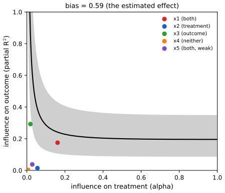
The book is careful about what such a plot can and cannot say. It rests on (36.105), which imposes a parametric form on the relation of \(U\) with \(A\) and \(Y\) that has no substantive justification; so Austen plots are useful where the conclusion is obvious to a domain expert (an unobserved confounder like socioeconomic status would not change the qualitative finding), and not for statements such as "a latent confounder could only be 90 percent as strong as age, so there is a small non-zero effect". Many other sensitivity models allow any machine learning model for the data analysis, but none is yet routine. The calibration needs care: it conditions on \(X\setminus Z\), whereas the hidden confounder acts given all of \(X\). Cinelli and Hazlett (2020) give an example where \(Z\) and \(U\) are the same variable but the influence of \(U\) given \((A,X)\) exceeds that of \(Z\) given \((A,X\setminus Z)\); and if \(U\) and \(Z\) are independent and both influence \(A\), then conditioning on the collider \(A\) creates an interaction. Conversely, if \(U\) and \(Z\) are dependent (race and wealth), omitting \(U\) increases the apparent importance of \(Z\), a conservative dot. An analyst should be sceptical whenever a strong confounder is believed to be omitted. The Austen demonstration reproduces the plot of Figure 36.7 and lets you move a hypothetical confounder across it.
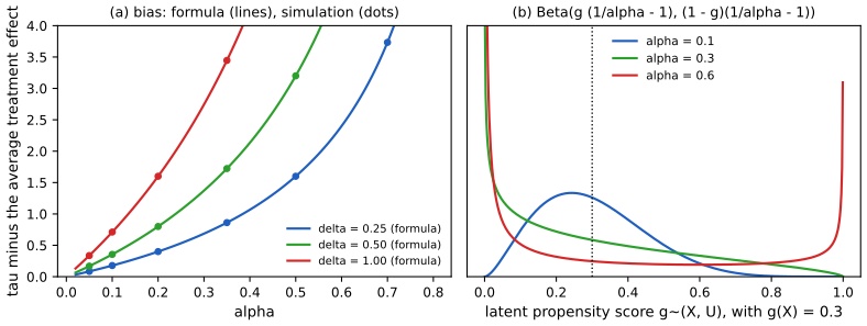
36.8 The do-calculus
pp. 1228–1232, (36.107)–(36.115), Figure 36.8 Confounder adjustment relied only on the assumed causal graph, whereas instruments and difference in differences also needed partial functional-form assumptions, which are hard to justify. It is natural to ask when the graph alone suffices. The do-calculus (Pearl) gives three rewrite rules which, when identification is possible, reduce an expression with \(\do\) to one with only observed quantities. With \(X,Y,Z,W\) disjoint sets of nodes of a causal DAG \(G\), \(G_{\overline X}\) the graph with the arrows into \(X\) removed and \(G_{\underline Z}\) the graph with the arrows out of \(Z\) removed:
- Rule 1 (insert or delete observations): \(p(y\given\do(x),z,w)=p(y\given\do(x),w)\) if \((Y\indep Z\given X,W)\) in \(G_{\overline X}\) (36.107).
- Rule 2 (exchange action and observation): \(p(y\given\do(x),\do(z),w)=p(y\given\do(x),z,w)\) if \((Y\indep Z\given X,W)\) in \(G_{\overline X\underline Z}\) (36.108). The simplest case is a root \(Z\), where \(\do(z)\) is conditioning because the mutilated graph equals the original.
- Rule 3 (insert or delete actions): \(p(y\given\do(x),\do(z),w)=p(y\given\do(x),w)\) if \((Y\indep Z\given X,W)\) in \(G_{\overline X\,\overline{Z(W)}}\), where \(Z(W)\) is the set of \(Z\)-nodes that are not ancestors of any \(W\)-node in \(G_{\overline X}\) (36.109).
(The book's statement of the graphs is slightly informal: it writes \(G_{XZ}\) for the graph that cuts the arrows into \(X\) and out of \(Z\), and \(G_{XZ^*}\) for the one that cuts those into \(X\) and \(Z^*\).) Rule 1 is d-separation in the mutilated graph; the rules are theorems of Pearl (1995), quoted here.
Backdoor adjustment. If we observe all parents \(X\) of \(A\), \(p(y\given\do(a))=\sum_xp(y\given x,\do(a))p(x\given\do(a))=\sum_xp(y\given x,a)p(x)\) (36.110–36.111). Generally a set \(S\) satisfies the backdoor criterion if no node of \(S\) is a descendant of \(A\) and \(S\) blocks every backdoor path from \(A\) to \(Y\); then \[ p(y\given\do(a))=\E_S\bigl[p(y\given S,A=a)\bigr],\qquad\ATE=\E_S\bigl[\E[Y\given A=1,S]-\E[Y\given A=0,S]\bigr]. \tag{36.112} \] Both the parents of \(A\) and the set of all common causes satisfy it (Gap 36.10), so the estimators of Section 36.4 apply with \(S\) in place of \(X\). The requirement that \(S\) has no descendants of \(A\) protects against adjusting for mediators and colliders.
Front-door adjustment. Backdoor adjustment needs an observed variable on every backdoor path. In Figure 36.8 the effect of smoking \(A\) on cancer \(Y\) passes entirely through a mediator \(M\) (tar, tissue damage), and a latent genotype \(U\) confounds \(A\) and \(Y\). The effect of \(A\) on \(M\) and that of \(M\) on \(Y\) are both identified by backdoor adjustment, and combining them, \[ p(y\given\do(a))=\sum_mp(y\given\do(m))p(m\given\do(a))=\sum_m\sum_{a'}p(y\given a',m)\,p(a')\,p(m\given a). \tag{36.113--36.114} \] A set \(M\) satisfies the front-door criterion for \((A,Y)\) if (1) \(M\) intercepts all directed paths from \(A\) to \(Y\); (2) no unblocked backdoor path joins \(A\) and \(M\); (3) every backdoor path from \(M\) to \(Y\) is blocked by \(A\); with \(p(A,M)>0\) for all values the effect is identified by (36.114). In the smoking example, (1) says smoking affects cancer only via tar and tissue damage, (2) and (3) that the genotype acts on \(M\) only through smoking, and positivity that high tar must also arise from other causes (so \(p(A=0,M=1)>0\)). Estimation fits \(\hat p(y\given m,a)\), \(\hat p(m\given a)\), and the empirical \(\hat p(a)\) and plugs in (36.115); average-effect estimators follow, and Fulcher et al. (2020) give robust versions and generalisations.
Filling the gap 36.20: the backdoor formula from rules 3 and 2, and a direct proof of the front-door formula pp. 1229–1232
Proof
(i) Backdoor. Let \(S\) satisfy the backdoor criterion. By probability, \(p(y\given\do(a))=\sum_sp(y\given\do(a),s)\,p(s\given\do(a))\). Rule 3 gives \(p(s\given\do(a))=p(s)\): in \(G_{\overline A}\) (the arrows into \(A\) removed), \(A\) is connected only to its descendants, and \(S\) contains none, so \(A\) and \(S\) are d-separated with no conditioning. Rule 2 gives \(p(y\given\do(a),s)=p(y\given a,s)\) if \(Y\indep A\given S\) in \(G_{\underline A}\), the graph without the arrows out of \(A\); there every path between \(A\) and \(Y\) is a backdoor path, and \(S\) blocks all of them, which is the second half of the criterion. Hence (36.112). The parents-only case (36.110–36.111) is the special case \(S=\pa(A)\).
(ii) Front-door, directly. In the graph \(U\to A\to M\to Y\), \(U\to Y\) the joint is \(p(u,a,m,y)=p(u)p(a\given u)p(m\given a)p(y\given m,u)\). By the truncated factorisation (Gap 36.1), \(p(y\given\do(a))=\sum_{u,m}p(u)p(m\given a)p(y\given m,u)\). On the other side, \(y\indep a'\given m,u\) (the only path from \(A\) to \(Y\) is through \(M\)) and \(u\indep m\given a'\) (\(U\) reaches \(M\) only through \(A\)), so \[ p(y\given m,a')=\sum_up(y\given m,u)p(u\given m,a')=\sum_up(y\given m,u)p(u\given a'), \] and therefore \(\sum_{a'}p(a')p(y\given m,a')=\sum_up(y\given m,u)\sum_{a'}p(a')p(u\given a')=\sum_up(y\given m,u)p(u)\). Substituting, \(\sum_mp(m\given a)\sum_{a'}p(a')p(y\given m,a')=\sum_{m,u}p(m\given a)p(u)p(y\given m,u)=p(y\given\do(a))\), which is (36.114): all that remains on the left side is observable, although \(U\) is not.
(iii) A numerical example. Take binary variables with \(P(U=1)=\tfrac12\), \(P(A=1\given U)=0.2+0.6U\), \(P(M=1\given A)=0.1+0.7A\) and \(P(Y=1\given M,U)=0.1+0.5M+0.3U\). The truth is \(P(Y=1\given\do(A=0))=0.30\) and \(P(Y=1\given\do(A=1))=0.65\), the ATE is 0.35. The naive conditional risks, using only \((A,M,Y)\), are 0.21 and 0.74 (the naive contrast is 0.53), and the front-door formula (36.114) computed from the observed joint returns 0.30 and 0.65 to machine precision (Figure x36.5). ∎
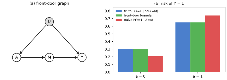
See also d-separation, Section 4.2.4.1, and constraint-based structure learning (S30.3.5), which estimates the graph that the do-calculus assumes known.
36.9 Further reading
pp. 1232–1233 The book points to textbooks with different emphases: Pearl (2009) for causal graphs, Angrist and Pischke (2008) for econometrics, Hernán and Robins (2020) for epidemiology, Imbens and Rubin (2015) for statistics, Morgan and Winship (2015) for the social sciences, and Shalizi (2022, Chapter 7) for a treatment of matching. Double machine learning is an instance of non-parametric estimation (Chernozhukov et al., 2017), with lucid explanations by Kennedy and by Fisher and Kennedy; estimators with the same asymptotics can differ in finite samples (van der Laan and Rose, 2011 for targeted estimators). The estimation of heterogeneous treatment effects (the effect for a given covariate profile) uses the same identification arguments but harder estimation. Other strategies: regression discontinuity (a sharp threshold in treatment assignment: compare units just below and just above), synthetic controls (a weighted average of untreated units balancing demographics, compared with the treated unit, for example for a smoking ban in California) and time-series versions of the idea (predict the untreated future of a series from its past and compare with what happened, Brodersen et al., 2015). Finally the book mentions the converse use of causality in machine learning: building predictors that are robust under domain shift or that avoid spurious correlations.
Practice problems
The chapter has no end-of-chapter exercises, so here are three short problems of my own, with complete solutions (hidden).
Practice problem 36.1 (LATE arithmetic). In a randomised encouragement design, \(P(A=1\given Z=1)=0.7\), \(P(A=1\given Z=0)=0.3\), \(\E[Y\given Z=1]=5.2\) and \(\E[Y\given Z=0]=4.4\). Assume the instrument conditions and monotonicity. (a) Find the shares of compliers, always takers and never takers and the LATE. (b) What can you conclude if the first stage were 0 while the difference \(\E[Y\given Z=1]-\E[Y\given Z=0]=0.8\)? (c) Why can the ATE not be found from these four numbers?
Solution
(a) By Gap 36.13, \(P(A=1\given Z=0)=P(\text{always})=0.3\) and the first stage is \(P(\text{complier})=0.7-0.3=0.4\), so never takers have share \(1-0.3-0.4=0.3\). The intention-to-treat effect is \(5.2-4.4=0.8=P(\text{complier})\cdot\LATE\), so \(\LATE=0.8/0.4=2.0\). (The Wald estimator, \(\text{ITT}/\text{first stage}\).) (b) Then \(Z\) changes the outcome without changing the treatment, so either the exclusion restriction or the unconfoundedness of the instrument must fail: a nonzero reduced form with a zero first stage is impossible under the instrument assumptions (the ITT equals \(P(\text{complier})\LATE=0\)). (c) The data constrain only the compliers' effect and the share of each type; always takers (30 percent) are never seen untreated-by-choice and never takers never treated, so their effects, and hence the ATE, are unrestricted. The ATE equals \(0.4\cdot2.0+0.3\theta_a+0.3\theta_n\) with arbitrary \(\theta_a,\theta_n\).
Practice problem 36.2 (difference in differences with a covariate). A policy hits restaurants of two types, 1 (cheap) and 2 (expensive). Mean changes \(\E[Y_1-Y_0]\): treated, type 1: 3.0, type 2: 1.0; controls, type 1: 1.0, type 2: \(-1.0\). The share of cheap restaurants is 0.4 among the treated and 0.8 among the controls. Compute the unadjusted difference in differences and the estimate (36.93), and explain the discrepancy.
Solution
Mean change of the treated: \(0.4\cdot3+0.6\cdot1=1.8\); of the controls: \(0.8\cdot1+0.2\cdot(-1)=0.6\); unadjusted difference in differences: \(1.8-0.6=1.2\). The adjusted estimate averages the within-type differences with the treated's type shares: \(0.4(3-1)+0.6(1-(-1))=0.8+1.2=2.0\). Under conditional parallel trends the counterfactual change of the treated is the controls' change type by type, \(0.4\cdot1+0.6\cdot(-1)=-0.2\), not the controls' overall average \(0.6\): the controls are mostly cheap restaurants, which trend upward, so the unadjusted estimator subtracts too much. The bias is \(1.2-2.0=-0.8=0.6-(-0.2)\) times \(-1\), the difference of the two counterfactual trends.
Practice problem 36.3 (an Austen bias). The propensity score is the constant \(g=0.25\), the confounder has \(\alpha=0.2\) and \(\delta=1.5\). (a) Find the bias of Theorem 6. (b) Find it for \(g=0.5\). (c) Find it if an instrument splits the population into two equal halves with \(g=0.1\) and \(g=0.4\).
Solution
The bias magnitude is \(|\delta|\frac{\alpha}{1-\alpha}\E[1/(g(1-g))]\) with \(\frac{\alpha}{1-\alpha}=0.25\). (a) \(1/(0.25\cdot0.75)=5.333\): bias \(=1.5\cdot0.25\cdot5.333=2.0\). (b) \(1/(0.5\cdot0.5)=4\): bias \(1.5\). (c) The mean propensity is still 0.25, but \(\E[1/(g(1-g))]=\tfrac12\bigl(1/0.09+1/0.24\bigr)=\tfrac12(11.11+4.167)=7.639\), so the bias is \(1.5\cdot0.25\cdot7.639=2.865\): conditioning on the instrument increases the bias by 43 percent for the same \(\alpha,\delta\), the z-bias of Gap 36.17(iv) (strict convexity of \(u\mapsto1/(u(1-u))\)). (b) also shows that the most balanced propensity (0.5) gives the smallest bias.
Demonstrations
- Adjusting for confounders (Section 36.4, Figure 36.3): one confounder, with the naive contrast, outcome regression, IPTW, Hajek and AIPTW estimators and their sampling distributions; change the confounding, the overlap and which nuisance model is wrong. Presets: 1 randomised, 3 wrong outcome model, 4 wrong propensity model, 6 poor overlap.
- Instruments and the local average treatment effect (Section 36.5.2, Figure x36.3): compliers, always takers, never takers and defiers; the as-treated contrast, the intention-to-treat effect and the Wald estimator; weak instruments, defiers and exclusion violations.
- Austen plots (Section 36.7.2, Figure 36.7): the bias formula, the curve of confounding strengths giving a chosen bias, and the calibration against observed covariates, on the simulated study.
Python code for every figure: code index. Data used by the demonstrations: data/ch36-observational.json, data/ch36-iv.json, data/ch36-austen.json. Companion: All of Statistics, Chapter 16; causal discovery demonstrations of Chapter 30.
Notes on the book
Points where the chapter is imprecise or wrong
- (36.37)–(36.38), page 1202. The error of the AIPTW estimator is \(\E[\frac{\hat g-g}{\hat g}(\hat Q_1-Q_1)+\frac{\hat g-g}{1-\hat g}(\hat Q_0-Q_0)]\): the denominators are \(\hat g\) and \(1-\hat g\), not \(g\) and \(1-g\) (gap 36.6: on an exact example the printed form gives \(-0.073\) where the true error is \(0.306\)).
- Page 1202, the condition for the root-\(n\) rate. "The product of the misestimation errors is \(o(\sqrt n)\)" should be \(o(n^{-1/2})\), and the displayed condition before (36.39), \(\sqrt n\,\E(\hat Q-Q)^2\E(\hat g-g)^2\to0\), lacks the exponent \(\tfrac12\) on each mean square (it would permit \(n^{-1/8}\) rates). The same slip, \(o(\sqrt n)\), is in the LATE condition on page 1214 (gaps 36.6, 36.14).
- (36.59) and (36.69), pages 1212–1213. Both write \(\E[Y\given\do(Z=1)]-\E[Y\given\do(Z=1)]\); the second term should have \(\do(Z=0)\) (gap 36.13).
- Page 1224, the bias. The bias is defined as \(\ATE-\tau\) and written with a positive sign, \(\delta(\E[\logit\tilde g\given X,A=1]-\E[\logit\tilde g\given X,A=0])\). The ATE equals \(\tau\) minus that quantity, so \(\ATE-\tau\) is negative for \(\delta>0\) (the hidden confounder inflates the observed contrast); Theorem 6 gives the right magnitude (gap 36.17, simulation).
- (36.102), page 1224. \(\alpha=\E[\tilde g\given A=1]-\E[\tilde g\given A=0]\) holds conditionally on \(X\), not unconditionally (for \(g\in\{0.2,0.8\}\), \(\alpha=0.3\) the unconditional difference is 0.552; gap 36.18).
- Figure 36.1(a). The text speaks of 1931; the title printed in the panel reads "USA, 2020".
- (36.83), page 1215. The covariate terms \(\delta_AX+\gamma_AX\) (and \(\delta_YX+\gamma_YX\) in (36.84)) repeat the same product; one coefficient vector per equation is meant.
References
Keys of the book's bibliography are in square brackets where it uses them.
- Murphy, K. P. (2023). Probabilistic Machine Learning: Advanced Topics. MIT Press, Cambridge, MA. Chapter 36 (Victor Veitch and Alex D'Amour), pp. 1185–1233. probml.github.io/pml-book/book2.html.
- [AP08] Angrist, J. D. and Pischke, J.-S. (2008). Mostly Harmless Econometrics. Princeton University Press. [AIR96] Angrist, J. D., Imbens, G. W. and Rubin, D. B. (1996). Identification of causal effects using instrumental variables. Journal of the American Statistical Association, 91(434), 444–455.
- [CK94] Card, D. and Krueger, A. B. (1994). Minimum wages and employment: a case study of the fast-food industry in New Jersey and Pennsylvania. American Economic Review, 84(4), 772–793.
- [Che+17] Chernozhukov, V., Chetverikov, D., Demirer, M., Duflo, E., Hansen, C., Newey, W. and Robins, J. (2018). Double/debiased machine learning for treatment and structural parameters. The Econometrics Journal, 21(1), C1–C68.
- [CH20] Cinelli, C. and Hazlett, C. (2020). Making sense of sensitivity: extending omitted variable bias. Journal of the Royal Statistical Society, Series B, 82(1), 39–67.
- [Cor+59] Cornfield, J., Haenszel, W., Hammond, E. C., Lilienfeld, A. M., Shimkin, M. B. and Wynder, E. L. (1959). Smoking and lung cancer: recent evidence and a discussion of some questions. Journal of the National Cancer Institute, 22(1), 173–203.
- [Imb03] Imbens, G. W. (2003). Sensitivity to exogeneity assumptions in program evaluation. American Economic Review, 93(2), 126–132. [IA94] Imbens, G. W. and Angrist, J. D. (1994). Identification and estimation of local average treatment effects. Econometrica, 62(2), 467–475. [IR15] Imbens, G. W. and Rubin, D. B. (2015). Causal Inference for Statistics, Social, and Biomedical Sciences. Cambridge University Press.
- [KS07] Kang, J. D. Y. and Schafer, J. L. (2007). Demystifying double robustness: a comparison of alternative strategies for estimating a population mean from incomplete data. Statistical Science, 22(4), 523–539.
- Kinal, T. W. (1980). The existence of moments of k-class estimators. Econometrica, 48(1), 241–249.
- Newey, W. K. and Powell, J. L. (2003). Instrumental variable estimation of nonparametric models. Econometrica, 71(5), 1565–1578.
- [Pea09] Pearl, J. (2009). Causality, 2nd edition. Cambridge University Press. Pearl, J. (1995). Causal diagrams for empirical research. Biometrika, 82(4), 669–688.
- Robins, J. M., Rotnitzky, A. and Zhao, L. P. (1994). Estimation of regression coefficients when some regressors are not always observed. Journal of the American Statistical Association, 89(427), 846–866. Rosenbaum, P. R. and Rubin, D. B. (1983). The central role of the propensity score in observational studies for causal effects. Biometrika, 70(1), 41–55.
- van der Vaart, A. W. (1998). Asymptotic Statistics. Cambridge University Press.
- [VS11] VanderWeele, T. J. and Shpitser, I. (2011). A new criterion for confounder selection. Biometrics, 67(4), 1406–1413.
- [VZ20] Veitch, V. and Zaveri, A. (2020). Sense and sensitivity analysis: simple post-hoc analysis of bias due to unobserved confounding. Advances in Neural Information Processing Systems, 33.
- Wasserman, L. (2004). All of Statistics. Springer (Chapter 16, see the companion notes).
The numerical statements in the text (the truncated factorisation and the risk differences of the smoking model; the non-identifiable pair of models; the decomposition of the naive contrast; the inverse weighting identity; the double robustness and the exact error of the augmented estimator; the efficiency bound; the coverage of the cross-fitted and randomised-trial intervals; the equality of matching and the saturated regression; balancing scores; the ATT with failing overlap; the closed forms for M-bias, a mediator and a collider; the equality of the Wald and two stage least squares estimators, the principal-strata limits with defiers and exclusion violations, the additive-confounding integral equation; the rate and coverage of the double machine learning estimators; difference in differences, its regression form and its bias; the Beta identities, the bias formula, the trigamma formula and the plateau of the Austen model; z-bias and placebo values; the front-door formula) were confirmed numerically by exact enumeration or simulation.