Representation learning
A representation is a transformation of raw inputs chosen so that tasks we have not yet seen become easy. Nobody can write down the transformation directly, so the field designs a surrogate task whose solution forces the network to build a useful one: predict labels, reconstruct or denoise the input, predict a hidden part of it, or make two views of the same example agree. These notes prove what the book states without proof about each stage: how to compare two representations (centred kernel alignment and canonical correlations, with their invariances and their failure when there are more neurons than examples), what a linear autoencoder and a denoising autoencoder actually learn, why InfoNCE is a bound on mutual information and what its gradient does, why collapse is a global minimum that Barlow Twins, BYOL and DINO avoid, and why a factorial latent model cannot be identified from the data law alone. Small experiments on the scikit-learn digits compare the pretext tasks by linear evaluation.
Ch. 1 Introduction Ch. 2 Probability Ch. 3 Statistics Ch. 4 Graphical models Ch. 5 Information theory Ch. 6 Optimisation Ch. 7 Inference algorithms Ch. 8 Gaussian filtering Ch. 9 Message passing Ch. 10 Variational inference Ch. 11 Monte Carlo Ch. 12 MCMC Ch. 13 Sequential Monte Carlo Ch. 14 Predictive models Ch. 15 GLMs Ch. 16 Deep networks Ch. 17 Bayesian neural networks Ch. 18 Gaussian processes Ch. 19 Beyond iid Ch. 20 Generative models Ch. 21 VAEs Ch. 22 Autoregressive models Ch. 23 Normalizing flows Ch. 24 Energy-based models Ch. 25 Diffusion models Ch. 26 GANs Ch. 27 Discovery methods Ch. 28 Latent factor models Ch. 29 State-space models Ch. 30 Graph learning Ch. 31 Nonparametric Bayes Ch. 32 Representation learning Ch. 33 Interpretability Ch. 34 Decision making Ch. 35 Reinforcement learning Ch. 36 Causality
How to read these notes
They follow the book. Sections carry the book's numbers, and equations the book numbers keep their numbers, e.g. \((32.17)\); equations without a number are steps the book skips. The online supplement has no content for this chapter (see S32).
Filling the gaps. Wherever the book writes "it can be shown", quotes a result from the literature, or leaves a step to the reader, an orange Filling the gap box gives the full argument. Proofs start hidden: open one with its bar, or use the buttons below. Results already proved elsewhere on the site (the principal subspace of a linear autoencoder, the optimal denoiser and Tweedie's formula, the InfoNCE bound by the variational route, the Eckart–Young theorem) are stated and linked, and the boxes spend their space on what this chapter adds: the invariances and the rank structure of CKA and CCA, the exact relation of three similarity indexes to regression, why regularised linear evaluation depends on the basis, an independent proof of the InfoNCE bound with K = M + 1 candidates, the gradient and the zero-temperature limit of InfoNCE, a one-mode model in which BYOL's collapse can be computed, and an explicit entangling map behind the non-identifiability theorem.
Figures, scale and demonstrations. Every computed figure is reproduced by the Python code (numpy, scikit-learn and PyTorch on one CPU thread; the figures take about six minutes in all). Figures 32.2 to 32.5 are diagrams and photographs and are not reproduced; Figure 32.1 is redrawn from two small networks; seven figures marked (own) go beyond the book. The numbers in the text come from these experiments. Three interactive demonstrations are linked where their topics arise.
Main reference
K. P. Murphy, Probabilistic Machine Learning: Advanced Topics, MIT Press (2023; online draft of December 2025), Chapter 32, pages 1049–1071, written by Ben Poole and Simon Kornblith (book page: probml.github.io/pml-book/book2.html), and the supplementary material, Chapter 32, pages 301–302 (a chapter heading only). Section, equation, figure and algorithm numbers below refer to this book.
Companion courses
Volume 1 treats representation learning from the label-efficiency side: transfer learning and fine-tuning, SimCLR and the InfoNCE bound by the variational route and the CLIP loss. The deep-learning course proves the principal-subspace property of linear autoencoders, the optimal denoiser and Tweedie's formula and the optimal denoiser for masking noise, and has a linear autoencoder demonstration. In this volume, Section 5.6.1 and gap 5.23 derive the information bottleneck, Section 21.3.1.1 discusses disentangled VAEs, Section 28.3.4 treats canonical correlation analysis as a probabilistic model, Section 28.6.2 independent component analysis, Section 16.3.3 autoencoders, Section 19.5.1 transfer learning, Section S3.3 Tweedie's formula and gap 26.13 BiGAN.
What this chapter adds: the rank and invariance structure of CKA and CCA (and the identification of three indexes of Section 32.2.2.2 with regression), the dependence of regularised linear evaluation on the basis, the precise statement of what a linear autoencoder and a linear denoising autoencoder learn, an independent proof of the InfoNCE bound, the gradient and temperature limits of InfoNCE, the collapse analysis of Barlow Twins, BYOL and DINO, the explicit entangling map behind the identifiability theorem, and the facts about deterministic encoders and mutual information estimators; plus an experiment that compares twelve learners and baselines on the same data.
The chapter at a glance
- 32.1 What a representation is for; Figure 32.1 redrawn with two small networks.
- 32.2.1 Linear evaluation is not invariant to the basis of the representation (gap 32.1).
- 32.2.2 Centred kernel alignment and its identity (32.2) (gap 32.2); CCA by QR and SVD, invariances, the curse of dimensionality and its exact size (32.3); SVCCA, PWCCA and their invariances (32.4); the identities (32.9)–(32.12) and a correction to the condition for (32.9) (32.5).
- 32.3.2–32.3.3 What linear autoencoders learn (gap 32.6); denoising and masked prediction as conditional means (32.7).
- 32.3.4 The InfoNCE bound (gap 32.8) and its gradient (32.9); Barlow Twins (32.10); BYOL and SimSiam in a one-mode model (32.11); DINO (32.12).
- 32.4 The entangling map behind non-identifiability (gap 32.13); infinite information, estimator ceilings and InfoMax (32.14).
Notation. \(X\in\R^{n\times p_1}\) and \(Y\in\R^{n\times p_2}\) are representation matrices of the same \(n\) examples, \(H=I-\tfrac1n\bm 1\bm 1^\T\) centres the rows, \(\tilde X=HX\), \(\tilde Y=HY\). \(\Fn{\cdot}\) is the Frobenius norm. For a pair \((x,y)\), \(\MI(X;Y)\) is mutual information in nats, \(r(x,y)=p(y\given x)/p(y)\) the density ratio. Learned maps are \(f_\theta\) (encoder) and \(g_\phi\) (decoder or second tower).
Prerequisites. Chapter 5 of the book (KL divergence, mutual information), Chapter 16 (autoencoders) and Volume 1, Chapters 7 and 20 (linear algebra, dimensionality reduction).
32.1 Introduction
p. 1049 Supervised learning fixes the task at training time. A representation is meant for the opposite situation: we learn a map \(\bm z=f_\theta(\bm x)\) before we know which questions will be asked, hoping that the right questions become easy in \(\bm z\) (a few labelled examples suffice, nearby points are similar, nuisance information is gone). The difficulty is that "useful for unknown tasks" cannot be turned into a loss, so every method replaces it by a surrogate task: classify, reconstruct, predict a masked part, or pull two views together. The book groups the surrogate tasks into supervised, generative and self-supervised (Section 32.3), after first fixing how a representation is judged (Section 32.2), and ends with theory (Section 32.4).
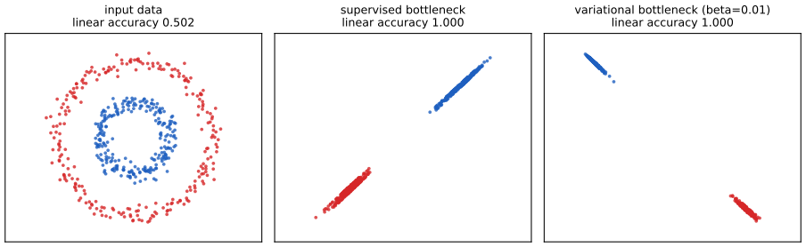
See also: variational information bottleneck (this volume) and transfer learning (Volume 1).
32.2 Evaluating and comparing learned representations
pp. 1049–1050 A representation lives in a high-dimensional space, so any judgement of its quality summarises it by a few scalars. Two families of summaries are used: how well the representation serves a task (Section 32.2.1), and how it relates to another representation, with no task in sight (Section 32.2.2). Each summary builds in an assumption about which structure matters, and the theorems below make those assumptions explicit as invariances.
32.2.1 Downstream performance
p. 1050 Downstream performance means adapting the representation to one or more tasks believed typical. The downstream task can share the input distribution with pretraining (labels that pretraining ignored, as when ImageNet images are used without labels for pretraining and with labels for evaluation) or differ in it (transfer learning, Section 19.5.1).
32.2.1.1 Linear classifiers and linear evaluation
pp. 1050–1051 In linear evaluation the network is frozen and a linear classifier, today usually an \(\ell_2\)-regularised multinomial logistic regression, is trained on the features of one layer. The problem is convex, so with all features in memory a full-batch quasi-Newton method (L-BFGS) with a warm start along the regularisation path is reliable, whereas stochastic gradient descent needs tuned schedules and many epochs. The book's remark that "even an invertible linear transformation of a representation can affect linear evaluation accuracy" is exact and easy to quantify.
Filling the gap 32.1: regularised linear evaluation depends on the basis of the representation pp. 1050–1051
Proof
Claim. Let \(Z=XA\) with \(A\in\R^{d\times d}\) invertible, and consider the \(\ell_2\)-regularised linear problem \(\min_{\bm\beta}\ \ell(Z\bm\beta;\bm y)+\lambda\|\bm\beta\|^2\) for any loss \(\ell\) that depends on the features only through the scores. Writing \(\bm w=A\bm\beta\), the scores are \(Z\bm\beta=X\bm w\) and \(\|\bm\beta\|^2=\bm w^\T(AA^\T)^{-1}\bm w\). So the problem in the new coordinates is the problem in the old ones with the penalty \(\lambda\,\bm w^\T(AA^\T)^{-1}\bm w\) instead of \(\lambda\|\bm w\|^2\): the data term is basis free, the penalty is not.
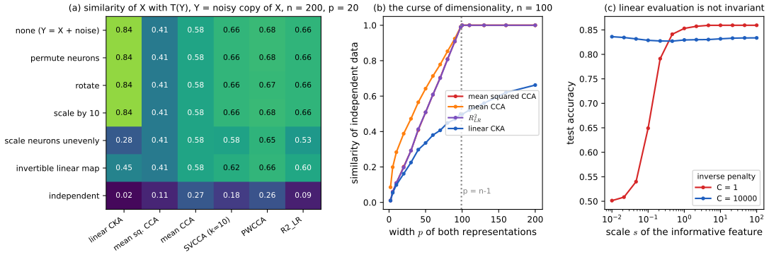
When are the predictions unchanged? For ridge regression with \(X=I_d\) (so \(n=d\)) and arbitrary \(\bm y\), the old fit is \(\hat{\bm y}=(1+\lambda)^{-1}\bm y\) and the new fit is \(A(A^\T A+\lambda I)^{-1}A^\T\bm y=(I+\lambda(AA^\T)^{-1})^{-1}\bm y\). These agree for every \(\bm y\) and \(\lambda\) iff \((AA^\T)^{-1}=I\), i.e. \(A\) is orthogonal. For \(A=cQ\) with \(Q\) orthogonal the effect is only to replace \(\lambda\) by \(\lambda/c^2\). Orthogonal maps (rotations, permutations of neurons) are therefore harmless, a uniform rescaling is harmless once \(\lambda\) is re-tuned, and everything else is not. As \(\lambda\to0\) with a unique minimiser the dependence disappears, because then only the data term remains.
A one-coordinate example. Multiplying a single feature by \(s\) divides its weight by \(s\) and so multiplies the effective penalty on the corresponding coefficient by \(1/s^2\): a feature scaled down by a factor 10 is penalised 100 times more, and the classifier ignores it. Panel (c) of Figure 32.x.a shows this on a two-class problem with one informative coordinate among ten and 60 training points: with \(C=1\) the test accuracy rises from 0.50 (at \(s=0.01\)) to 0.86 (\(s\ge1\)), while with \(C=10^4\) (almost no regularisation) it stays near 0.83 for every \(s\). Both statements were confirmed numerically (ridge predictions equal under orthogonal maps and differ under a diagonal rescaling; the transformed problem equals the old one with the penalty \(\bm w^\T(AA^\T)^{-1}\bm w\)).
32.2.1.2 Fine-tuning
pp. 1051–1052 Fine-tuning attaches a new head and updates every parameter on the downstream data, usually at a smaller learning rate than pretraining. It costs a backward pass through the whole network but beats linear evaluation except when there are very few labelled examples per class (about five in the cited studies). Variants keep the old weights fixed and add capacity: Net2Net widens a network while preserving its function, and adapter modules insert small trainable blocks, so only the adapters need storing per task (adapters in Volume 1). Detection and segmentation add a feature pyramid network that combines several layers. There is nothing here to prove; the experiment of Figure 32.x.e shows the few-label regime for linear evaluation.
32.2.1.3 Disentanglement
p. 1052 When the data are generated from known factors of variation (position, shape, colour) one can ask whether each factor is recovered by a single coordinate of the representation. Most metrics measure how close the dependence between factors and coordinates is to a one-to-one correspondence. Whether such a representation can be learned at all is the subject of Section 32.4.1; the models are in Section 21.3.1.1.
32.2.2 Representational similarity
p. 1052 Here two fixed representations of the same \(n\) examples are compared directly: \(X\in\R^{n\times p_1}\) and \(Y\in\R^{n\times p_2}\), possibly from different layers or networks and with different widths. Rows are examples, columns are neurons. Neurons have no canonical order, so any sensible index must at least ignore permutations of columns.
32.2.2.1 Representational similarity analysis and centered kernel alignment
pp. 1052–1053 Representational similarity analysis (RSA) compares the \(n\times n\) matrices of pairwise similarities between examples, \(K_{ij}=k(X_{i,:},X_{j,:})\) and \(K'_{ij}=k'(Y_{i,:},Y_{j,:})\), through a matrix similarity \(s(K,K')\); the common choice is the Spearman correlation of the entries. Centred kernel alignment (CKA) takes positive semi-definite kernels and the cosine similarity of the centred kernel matrices, \[ s(K,K')=\frac{\langle HKH,HK'H\rangle_{\mathrm F}}{\Fn{HKH}\,\Fn{HK'H}}, \tag{32.1} \] and for the linear kernel \(K=XX^\T\) it can be written with feature-feature matrices, \[ s(K,K')=\frac{\langle\tilde X\tilde X^\T,\tilde Y\tilde Y^\T\rangle_{\mathrm F}}{\Fn{\tilde X\tilde X^\T}\Fn{\tilde Y\tilde Y^\T}}=\frac{\Fn{\tilde X^\T\tilde Y}^2}{\Fn{\tilde X^\T\tilde X}\,\Fn{\tilde Y^\T\tilde Y}}. \tag{32.2} \]
Filling the gap 32.2: the identity (32.2), the range of CKA and its invariances pp. 1052–1053
Proof
The identity. \(H\) is symmetric and idempotent, so for \(K=XX^\T\), \(HKH=(HX)(HX)^\T=\tilde X\tilde X^\T\), and likewise for \(Y\). By the cyclic property of the trace, \(\langle\tilde X\tilde X^\T,\tilde Y\tilde Y^\T\rangle_{\mathrm F}=\Tr(\tilde X\tilde X^\T\tilde Y\tilde Y^\T)=\Tr(\tilde X^\T\tilde Y\tilde Y^\T\tilde X)=\Fn{\tilde X^\T\tilde Y}^2\), and \(\Fn{\tilde X\tilde X^\T}^2=\Tr(\tilde X\tilde X^\T\tilde X\tilde X^\T)=\Fn{\tilde X^\T\tilde X}^2\). This is (32.2). Dividing numerator and denominator by \(n^2\) turns it into \(\Tr(\Sigma_{XY}\Sigma_{YX})/\sqrt{\Tr(\Sigma_{XX}^2)\Tr(\Sigma_{YY}^2)}\) with the sample (cross-)covariances, the RV coefficient of Robert and Escoufier (1976), as the book says.
Range. For symmetric positive semi-definite \(A,B\): \(\langle A,B\rangle_{\mathrm F}=\Tr(A^{1/2}BA^{1/2})\ge0\), and Cauchy–Schwarz in the Frobenius inner product gives \(\langle A,B\rangle\le\Fn A\Fn B\). Hence \(0\le\mathrm{CKA}\le1\), with \(\mathrm{CKA}=1\) iff \(HKH\) and \(HK'H\) are proportional. In particular \(\mathrm{CKA}(X,X)=1\).
Invariances (linear kernel). If \(Y\to YQ\) with \(Q\) orthogonal, \(\tilde Y\tilde Y^\T\) is unchanged, and \(Y\to cY\) multiplies numerator and denominator by \(c^2\): CKA is invariant to rotations, permutations and one overall scale. It is not invariant to an invertible linear map \(A\): then \(\tilde Y\tilde Y^\T\to\tilde Y AA^\T\tilde Y^\T\), which reweights directions. Numerical example (confirmed): for \(n=120\) and a 15-neuron structured representation and a 12-neuron noisy linear image, CKA is 0.809, unchanged by rotation and scaling, and 0.440 after a condition-number-100 linear map. By (32.12) below CKA weights the overlap of principal components by the products of their variances, which is why it is dominated by the leading directions.
See also: the kernel trick and positive semi-definite matrices in Volume 1, Chapter 17.
32.2.2.2 Canonical correlation analysis and related methods
pp. 1053–1055 Canonical correlation analysis (CCA) finds weight vectors \((\bm w_i,\bm w_i')\) such that the canonical variates \(\tilde X\bm w_i\) and \(\tilde Y\bm w'_i\) have the largest possible correlation, successively, with each new variate orthogonal to the previous ones in its own representation: \[ \operatorname*{maximise}\ \corr[\tilde X\bm w_i,\tilde Y\bm w_i']\quad\text{s.t. }\ \tilde X\bm w_i\perp\tilde X\bm w_j,\ \tilde Y\bm w'_i\perp\tilde Y\bm w'_j\ (j<i),\ \ \|\tilde X\bm w_i\|=\|\tilde Y\bm w'_i\|=1. \tag{32.3} \] The usual algorithm (Björck and Golub, 1973) factorises \(\tilde X=QR\), \(\tilde Y=Q'R'\) with \(Q,Q'\) having orthonormal columns, takes an SVD \(Q^\T Q'=U\Sigma V^\T\), and reads off the canonical correlations \(\rho=\operatorname{diag}\Sigma\), the canonical variates \(QU\) and \(Q'V\) and the weights \(W=R^{-1}U\), \(W'=R'^{-1}V\). Two scalar summaries are the mean squared and the mean canonical correlation, \[ R^2_{\mathrm{CCA}}(X,Y)=\|\rho\|_2^2/p=\Fn{Q^\T Q'}^2/p,\qquad \bar\rho=\sum_{i=1}^p\rho_i/p=\|Q^\T Q'\|_*/p , \tag{32.4}\ (32.5) \] with \(p=\min(\rank X,\rank Y)\) and \(\|\cdot\|_*\) the nuclear norm.
Filling the gap 32.3: why the SVD of \(Q^\T Q'\) solves (32.3); invariances; the curse of dimensionality and its size pp. 1053–1054
Proof
Algorithm. Let \(r=\rank\tilde X\), \(r'=\rank\tilde Y\), so \(Q\in\R^{n\times r}\), \(R\in\R^{r\times p_1}\) has full row rank \(r\) (and likewise \(Q',R'\)). For a weight vector \(\bm w\) put \(\bm a=R\bm w\in\R^r\); as \(\bm w\) ranges over \(\R^{p_1}\), \(\bm a\) ranges over all of \(\R^r\), and \(\|\tilde X\bm w\|=\|Q\bm a\|=\|\bm a\|\), \(\langle\tilde X\bm w_i,\tilde X\bm w_j\rangle=\langle\bm a_i,\bm a_j\rangle\). With \(\bm b=R'\bm w'\) the correlation of two variates is \(\bm a^\T Q^\T Q'\bm b/(\|\bm a\|\|\bm b\|)\) and (32.3) becomes: maximise \(\bm a_i^\T M\bm b_i\) for unit, mutually orthogonal sequences \(\bm a_i\), \(\bm b_i\), where \(M=Q^\T Q'\). This is the variational characterisation of the SVD: the maximum of \(\bm a^\T M\bm b\) over unit vectors is \(\sigma_1(M)\), attained at the top singular pair, and under orthogonality to the earlier pairs the maximum is \(\sigma_i(M)\) (Courant–Fischer). So \(\rho_i=\sigma_i(M)\), the variates are \(Q\bm u_i\) and \(Q'\bm v_i\), and a weight vector solving \(R\bm w=\bm u_i\) is \(\bm w=R^{+}\bm u_i\) (equal to \(R^{-1}\bm u_i\) when \(R\) is square; it is not unique if \(p_1>r\)). All correlations lie in \([0,1]\) because \(\|M\|_2\le\|Q\|_2\|Q'\|_2=1\).
A projector form. \(\Fn{Q^\T Q'}^2=\Tr(Q^\T Q'Q'^\T Q)=\Tr(P_XP_Y)\), with \(P_X=QQ^\T\), \(P_Y=Q'Q'^\T\) the orthogonal projectors onto the two (centred) column spaces. So \(R^2_{\mathrm{CCA}}=\Tr(P_XP_Y)/p\) depends on the data only through the two column spaces, and the number of unit canonical correlations is \(\dim(\operatorname{col}\tilde X\cap\operatorname{col}\tilde Y)\).
Invariances. If \(X\to XG\) with \(G\) invertible, the column space, hence \(P_X\), is unchanged, so every canonical correlation, \(R^2_{\mathrm{CCA}}\) and \(\bar\rho\) are invariant to all invertible linear maps of either representation (permutations, rotations and rescalings included); this is the strongest invariance in the family, and the reason (32.4) and (32.5) cannot tell a representation from an arbitrary invertible linear image of it. Confirmed numerically, together with agreement of the first three correlations with an independent CCA routine.
The curse of dimensionality, exactly. Centring removes the direction \(\bm 1\), so \(\operatorname{col}\tilde X\subseteq\bm 1^\perp\), an \((n-1)\)-dimensional space, and \(r\le n-1\). If \(r=n-1\), i.e. \(X\) has at least \(n-1\) linearly independent neurons, then \(\operatorname{col}\tilde X=\bm 1^\perp\) contains \(\operatorname{col}\tilde Y\) for any \(Y\), so \(P_XP_Y=P_Y\), all \(r'\) canonical correlations equal 1 and \(R^2_{\mathrm{CCA}}=\bar\rho=1\), whatever \(Y\) is. (The book says "more neurons than examples"; \(n-1\) neurons already suffice, and only one of the two representations has to be wide.) Before that threshold the index is large for unrelated data too: if the columns of \(X\) and \(Y\) are independent Gaussian, \(\operatorname{col}\tilde Y\) is a uniformly random \(r'\)-dimensional subspace of \(\bm 1^\perp\) independent of \(P_X\), so \(\E P_Y=\frac{r'}{n-1}P_{\bm 1^\perp}\) and \[ \E\,\Tr(P_XP_Y)=\frac{r\,r'}{n-1},\qquad \E\,R^2_{\mathrm{CCA}}=\frac{\max(r,r')}{n-1}. \] For \(n=100\) and two independent \(p\)-neuron representations the mean squared canonical correlation is therefore about \(p/99\): 0.20 at \(p=20\), 0.51 at \(p=50\), 0.91 at \(p=90\) and 1.00 for \(p\ge99\), as in panel (b) of Figure 32.x.a. Linear CKA also grows with \(p\) for unrelated data (0.50 at \(p=100\)) but stays well below 1 and is not saturated by the threshold.
See also: CCA as a probabilistic model and as reduced-rank regression, gap 28.7.
p. 1054 To fight the curse, SVCCA keeps only the \(k\) leading principal components of each representation before running CCA (the book's (32.6) sets \(Q=U_{:,1:k}\), \(R=\Sigma_{1:k,1:k}V_{:,1:k}^\T\)); Raghu et al. choose \(k\) to explain 99% of the variance, but then representations with a slowly decaying spectrum need more components and look spuriously more similar to everything, so a common fixed \(k\) is better. Projection-weighted CCA averages the correlations with weights that measure how much of the second representation each canonical variate carries: \[ \mathrm{PWCCA}(X,Y)=\frac{\sum_{i=1}^p\alpha_i\rho_i}{\sum_{i=1}^p\alpha_i},\qquad \alpha_i=\|(\tilde Y\bm w_i')^\T\tilde Y\|_1 . \tag{32.7} \] Replacing the \(\ell_1\) norm by the squared \(\ell_2\) norm gives a rotation-invariant variant, \[ R^2_{\mathrm{LR}}(X,Y)=\frac{\sum_{i=1}^p\alpha_i'\rho_i^2}{\sum_{i=1}^p\alpha_i'},\qquad \alpha_i'=\|(\tilde Y\bm w_i')^\T\tilde Y\|_2^2 , \tag{32.8} \] (I read the printed \(\sum_{j}\) in \(\alpha_i'\) as the sum over the \(p_2\) neurons that the squared \(\ell_2\) norm already contains), and the book states that for \(p_2\ge p_1\) it equals the share of the variance of \(\tilde Y\) explained by regressing every neuron of \(\tilde Y\) on \(\tilde X\), \[ R^2_{\mathrm{LR}}(X,Y)=1-\sum_{i=1}^{p_2}\min_{\bm\beta}\|\tilde Y_{:,i}-\tilde X\bm\beta\|^2\big/\Fn{\tilde Y}^2 . \tag{32.9} \]
Filling the gap 32.4: what SVCCA and PWCCA are invariant to, why PWCCA is asymmetric, and the effect of \(k\) pp. 1054–1055, (32.6)–(32.7)
Proof
SVCCA. The principal components of \(\tilde X\) are its left singular vectors \(U\). For an orthogonal \(Q_o\), \(\tilde XQ_o=U\Sigma(Q_o^\T V)^\T\) is again an SVD with the same \(U\) and \(\Sigma\) (only the right singular vectors change), so \(U_{:,1:k}\) and hence the SVCCA correlations are unchanged: SVCCA is invariant to rotations, permutations and overall scale. An invertible non-orthogonal map changes the singular vectors \(U\) (it reweights directions before the SVD) and with it the top-\(k\) subspace, so SVCCA is not invariant to it (table in Figure 32.x.a, panel (a): rescaling neurons unevenly moves SVCCA from 0.66 to 0.58 while the canonical correlations stay put).
Monotone in \(k'\). For fixed \(Q_k\) (the top \(k\) components of \(X\)) and nested subspaces \(Q'_{k'}\subset Q'_{k''}\), the matrix \(Q_k^\T Q'_{k''}\) is \(Q_k^\T Q'_{k'}\) with extra columns appended; appending columns cannot decrease any singular value, because \(MM^\T\preceq[M\ m][M\ m]^\T\) in the Loewner order, so the \(i\)-th singular value is non-decreasing (Weyl's monotonicity). Hence for fixed \(\min(k,k')\) the CCA-based similarity can only grow with \(\max(k,k')\), as the book warns (numerically, 0.773, 0.888, 0.893 for \(k'=5,8,12\) and \(k=5\)).
PWCCA. Let \(\bm h_i=Q'\bm v_i\) be the \(i\)-th canonical variate of \(\tilde Y\). \(\alpha_i=\|\bm h_i^\T\tilde Y\|_1=\sum_j|\bm h_i^\T\tilde Y_{:,j}|\) sums absolute inner products with the individual neurons. Under \(\tilde Y\to\tilde YQ_o\) the vector \(\bm h_i\) is unchanged (the column space is the same) but the vector \((\bm h_i^\T\tilde Y_{:,j})_j\) is rotated, and the \(\ell_1\) norm is not rotation invariant (\(\|(1,0)\|_1=1\) but \(\|(\tfrac1{\sqrt2},\tfrac1{\sqrt2})\|_1=\sqrt2\)), so PWCCA changes. Numerically: 0.6649 for a noisy copy of a structured representation and 0.6697 after a random rotation of the copy. It is asymmetric because the weights come from \(Y\) only: \(\mathrm{PWCCA}(X,Y)=0.7994\) but \(\mathrm{PWCCA}(Y,X)=0.8015\) in the same example.
The \(\ell_2\) variant is rotation invariant. \(\alpha_i'=\bm h_i^\T\tilde Y\tilde Y^\T\bm h_i\) depends on \(\tilde Y\) only through \(\tilde Y\tilde Y^\T\), which is unchanged by \(\tilde Y\to\tilde YQ_o\); \(\bm h_i\) and \(\rho_i\) are unchanged too. Hence \(R^2_{\mathrm{LR}}\) is invariant to rotations (confirmed), and, like CKA, not to uneven rescalings (its \(\alpha'_i\) are variances).
Filling the gap 32.5: the identities (32.9)–(32.12), and the condition for (32.9) pp. 1055, (32.8)–(32.12)
Proof
Setup. Let \(\tilde X=U\Sigma V^\T\) and \(\tilde Y=U'\Sigma'V'^\T\) be thin SVDs with the numerical ranks \(r\), \(r'\), and put \(\lambda_i=\Sigma_{ii}^2\), \(\lambda'_j=\Sigma'^2_{jj}\) (the variances up to \(1/n\)). Take \(Q=U\), \(Q'=U'\), \(R'=\Sigma'V'^\T\).
Regression and (32.11). Regressing each column of \(\tilde Y\) on \(\tilde X\) gives the fitted matrix \(P_X\tilde Y=UU^\T\tilde Y\), so the variance explained is \(\|U^\T\tilde Y\|_{\mathrm F}^2/\Fn{\tilde Y}^2\) (the residual and the fit are orthogonal, so \(\Fn{\tilde Y}^2=\Fn{P_X\tilde Y}^2+\Fn{(I-P_X)\tilde Y}^2\)). Now \(U^\T\tilde Y=U^\T U'\Sigma'V'^\T\) and \(V'\) has orthonormal columns, so \(\|U^\T\tilde Y\|_{\mathrm F}^2=\|U^\T U'\Sigma'\|_{\mathrm F}^2=\sum_{i,j}\lambda'_j(\bm u_i^\T\bm u'_j)^2\) and \(\Fn{\tilde Y}^2=\sum_j\lambda'_j\). Hence the regression \(R^2\), the right-hand side of (32.9), equals \[ \frac{\sum_{i=1}^{p_1}\sum_{j=1}^{p_2}\lambda'_j(\bm u_i^\T\bm u_j')^2}{\sum_{j=1}^{p_2}\lambda'_j}, \tag{32.11} \] for every pair of ranks.
(32.8) versus (32.9). Let \(Q^\T Q'=U_c\operatorname{diag}(\rho)V_c^\T\) be the SVD of the canonical analysis, \(\bm h_i=Q'\bm v_{c,i}\), so \(\tilde Y^\T\bm h_i=R'^\T Q'^\T Q'\bm v_{c,i}=R'^\T\bm v_{c,i}\) and \(\alpha_i'=\|R'^\T\bm v_{c,i}\|^2\). Since \(U\) has orthonormal columns, \(\|U^\T\tilde Y\|^2_{\mathrm F}=\|Q^\T Q'R'\|_{\mathrm F}^2=\|\operatorname{diag}(\rho)V_c^\T R'\|_{\mathrm F}^2=\sum_i\rho_i^2\alpha_i'\). This is the numerator of (32.8) and of (32.9) (regression \(R^2\) times \(\Fn{\tilde Y}^2\)). The denominators are \(\sum_i\alpha_i'=\|V_c^\T R'\|_{\mathrm F}^2\) and \(\Fn{R'}^2=\Fn{\tilde Y}^2\). They are equal iff \(V_c\) (of size \(r'\times p\)) is an orthogonal square matrix, i.e. \(p=r'\): (32.8) equals (32.9) exactly when \(\rank\tilde Y\le\rank\tilde X\). In general \(\sum\alpha_i'\le\Fn{\tilde Y}^2\), so (32.8) \(\ge\) (32.9): when \(Y\) is the wider representation, some variance of \(Y\) lies outside the canonical directions and cannot be predicted from \(X\), and (32.8) ignores it. The book states the condition as \(p_2\ge p_1\), which is the reverse; with a 100-example, 8-neuron \(X\) and a 20-neuron \(Y\) we found 0.154 for (32.8) against 0.065 for (32.9), and 0.184 for both when \(X\) has 20 and \(Y\) has 8 neurons.
(32.10) and (32.12). With \(Q=U\), \(Q'=U'\): \(R^2_{\mathrm{CCA}}=\Fn{U^\T U'}^2/p=\sum_{i,j}(\bm u_i^\T\bm u'_j)^2/p\), which is (32.10) once \(p\) is read as \(\min(p_1,p_2)\) (the book divides by \(p_1\), correct for \(p_1\le p_2\)). For CKA, \(\tilde X^\T\tilde Y=V\Sigma U^\T U'\Sigma'V'^\T\) and \(V,V'\) have orthonormal columns, so \(\Fn{\tilde X^\T\tilde Y}^2=\Fn{\Sigma U^\T U'\Sigma'}^2=\sum_{i,j}\lambda_i\lambda'_j(\bm u_i^\T\bm u_j')^2\), while \(\Fn{\tilde X^\T\tilde X}^2=\Fn{V\Sigma^2V^\T}^2=\sum_i\lambda_i^2\). Inserting in (32.2) gives (32.12). All three indexes are sums over the overlaps \((\bm u_i^\T\bm u_j')^2\) of principal components, weighted by 1 (CCA), by \(\lambda'_j/\sum\lambda'\) (regression) and by \(\lambda_i\lambda'_j\) (CKA): the more variance a component has, the more it counts. Each identity (32.9)–(32.12), with the corrected condition, was confirmed numerically.
32.2.2.3 Comparing representational similarity measures
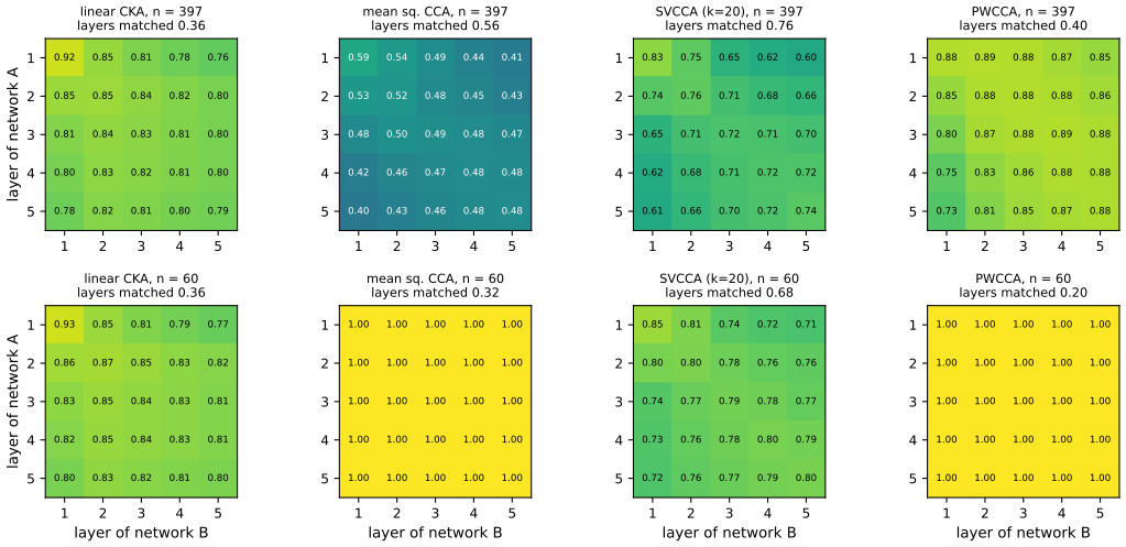
pp. 1055–1056 What a similarity index should be invariant to has no single answer. Permutations of neurons are the minimum (symmetric initialisations make every ordering equally likely). Invariance to every invertible map, which is what mutual information gives, is too much, because most trained networks are injective on their input, so an invertible map exists between any two layers. In practice indexes are invariant to rotations (CKA, SVCCA, \(R^2_{\mathrm{LR}}\)), to all invertible linear maps (the CCA correlations alone), or to neither (PWCCA with \(\ell_1\) weights). Kornblith et al. suggest an empirical sanity check: for two identical architectures trained from different initialisations, each layer of the first network should be most similar to the same layer of the second. CKA passed it for flattened convolutional features where other indexes failed; on Transformer tokens all indexes were adequate; and Maheswaranathan et al. found that CCA and CKA are both sensitive to harmless recurrent-network design choices.
32.3 Approaches for learning representations
pp. 1056–1057 The goal is a parametric map \(\bm z=f_\theta(\bm x)\) that makes future tasks easy, but since the tasks are unknown the training signal has to come from a proxy. The proxy must not be too easy (a shortcut solves it without learning anything interesting) nor too far from the downstream task (an object detector needs position, a classifier does not). The book's Figure 32.2 draws three families (supervised, generative, self-supervised) as a diagram; it contains nothing computed and is not reproduced. The experiment of Figure 32.x.e compares twelve learners and baselines on one data set.
32.3.1 Supervised representation learning and transfer
pp. 1057–1059 Networks trained on large labelled sets produced the first strong visual representations and remain the standard. Larger networks and datasets generally give better pretraining and downstream accuracy, but the correlation between the two weakens when the downstream domain differs (natural images to medical images); regularisers that help the pretraining task (dropout on the penultimate layer, label smoothing) can hurt transfer, whereas group normalisation with weight standardisation, adversarial training and a stronger weight decay on the last layer have helped it. To avoid human labels one uses weak supervision: hashtags, automatically generated labels, or captions. Image–text pairs allow word-prediction, captioning or masked-language objectives, and contrastive image–text pretraining (CLIP, ALIGN) learns two towers whose embeddings of matched pairs are close (Section 32.3.4.2); it also gives zero-shot classifiers built from the text of the class names, which are less accurate than a trained linear head but far more robust to distribution shift. There is no result to prove in this section; the CLIP loss and the zero-shot rule are derived in Volume 1. The experiment of Figure 32.x.e includes the supervised network as a reference for what labels buy.
32.3.2 Generative representation learning
p. 1059 Supervised features can fail for tasks that differ from the pretraining task, because they are trained to discard what the labels do not need (the style of a handwritten digit, for instance). Generative representation learning fits a model \(p_\theta(\bm x)\) of the whole data distribution in the hope that a model able to produce all the data must contain whatever any question would need. There are two routes: latent-variable models, whose latents (or an approximation to their posterior) are the representation, and fully observed models, from whose hidden layers a representation is read.
32.3.2.1 Latent-variable models
pp. 1059–1060 The principle is analysis by synthesis: if a model with few latent variables can synthesise the observations, the latents should track the factors that really generated them (position, size and type of a shape). Extraction means inference, \(\bm z\sim p_\theta(\bm z\given\bm x)\) or its mean. Greedy stacks of energy-based or sparse-coding models learned increasingly abstract features but did not scale to natural images. Where the generative process is known (strokes composing characters) building it in works very well; where it must be learned there is a trade-off between imposed structure (sparsity) and learned structure. Variational autoencoders (Chapter 21) learn a prior, a decoder and an amortised encoder \(q_\phi(\bm z\given\bm x)\) used to extract features on new points; \(\beta\)-VAEs recover factors of variation on simple synthetic data and VAEs help semi-supervised learning, but VAEs for natural images have not matched supervised or contrastive features. Adversarial models with an encoder (BiGAN, ALI) learn classification-quality features at small scale and BigBiGAN at ImageNet scale (gap 26.13 shows what the BiGAN optimum is).
32.3.2.2 Fully observed models
p. 1060 Autoregressive models (Chapter 22) or flows (Chapter 23) have no latent variables, yet their internal activations can be excellent features: ImageGPT, an autoregressive transformer on pixels, gives features that classify well, taken from a hidden layer rather than from a latent code. In language, masked training (BERT) typically beats left-to-right likelihood for representation quality.
32.3.2.3 Autoencoders
pp. 1060–1061 An autoencoder learns an encoder \(\bm z=f_\theta(\bm x)\) and a decoder \(g_\phi(\bm z)\) so that the input can be rebuilt, here with squared error, \[ L(\theta,\phi)=\frac1{|\mathcal D|}\sum_{\bm x\in\mathcal D}\|\bm x-g_\phi(f_\theta(\bm x))\|_2^2. \tag{32.13} \] Unlike a generative model it does not assign likelihoods or sample. Without constraints and with \(\dim\bm z=\dim\bm x\) the identity pair is optimal and nothing is learned, so the representation is restricted: by a smaller dimension, a sparsity penalty (\(\ell_1\) on \(\bm z\)), a smoothness penalty (contractive autoencoders), or noise added to the input or to hidden layers (denoising autoencoders, dropout). With linear maps and squared error the autoencoder "learns the principal components"; the precise statement is a little different.
Filling the gap 32.6: what a linear autoencoder learns: the principal subspace, not the components pp. 1060–1061, (32.13)
Proof
Statement. Let \(X\in\R^{n\times d}\) have sample covariance \(S=X^\T X/n\) with eigenvalues \(\lambda_1\ge\dots\ge\lambda_d\) and eigenvectors \(\bm v_i\), and fit \(\bm x\approx W_dW_e\bm x\) with \(W_e\in\R^{k\times d}\), \(W_d\in\R^{d\times k}\), \(k<d\), by minimising (32.13). Then the minimum is \(\sum_{i>k}\lambda_i\); if \(\lambda_k>\lambda_{k+1}\) and \(S\) is invertible the product \(M=W_dW_e\) is at every global minimum the orthogonal projector \(V_kV_k^\T\) onto the top-\(k\) eigenspace, \(\operatorname{col}W_d=\operatorname{col}V_k\), and the pair \((W_d,W_e)\) is determined only up to \((W_dG^{-1},GW_e)\) with \(G\in GL_k\); the columns of \(W_d\) need not be eigenvectors, nor orthogonal.
Proof. \(XM^\T\)-type products have rank at most \(k\), so by the Eckart–Young–Mirsky theorem (Result 7.5 of Volume 1) \(\Fn{X-XM^\T}\ge\Fn{X-X_k}\) where \(X_k=U_k\Sigma_kV_k^\T\) is the truncated SVD, with equality iff \(XM^\T=X_k\) when \(\sigma_k>\sigma_{k+1}\). The projector \(M=V_kV_k^\T\) attains it (\(XV_kV_k^\T=X_k\)), and since \(S\) is invertible \(X\) has full column rank, so \(XM^\T=X_k\) determines \(M\) uniquely. As \(\rank M=k\) forces \(\operatorname{col}M=\operatorname{col}W_d\) we get the claimed subspace. Any factorisation \(M=W_dW_e=(W_dG^{-1})(GW_e)\) is equally good, so the weights are fixed only up to \(G\); the deviation of \(W_d\) from the eigenvectors is therefore a property of the initialisation: along gradient flow \(\dot W_d=-2(M-I)SW_e^\T\), \(\dot W_e=-2W_d^\T(M-I)S\), one finds \(\tfrac{\d}{\d t}W_d^\T W_d=\tfrac{\d}{\d t}W_eW_e^\T=-2\big(W_e S(M-I)^\T W_d+W_d^\T(M-I)SW_e^\T\big)\), so \(W_d^\T W_d-W_eW_e^\T\) is conserved, and the limiting \(G\) is not forgotten. The deep-learning course gives the same statement and proof with more detail (Result 19.1); the nonlinear-hidden-units case is Result 19.2.
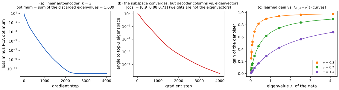
Numerical illustration. Ten-dimensional data with eigenvalues \((4,2.5,1.5,0.8,0.4,0.2,0.1,0.08,0.05,0.03)\), \(k=3\), full-batch gradient descent from a small random start with larger decoder than encoder weights: the loss reaches the Eckart–Young floor \(\sum_{i>3}\lambda_i=1.639\) (to \(10^{-15}\)), the largest sine of the principal angle between \(\operatorname{col}W_d\) and \(\operatorname{col}V_3\) falls below \(10^{-9}\), \(W_dW_e\) converges to the projector, and yet the cosines between the three decoder columns and the three eigenvectors are 0.90, 0.88 and 0.71 (Figure 32.x.c, (a) and (b)).
p. 1061 Other regularised autoencoders maintain a wide representation instead: sparse coding, contractive penalties, input noise, dropout. Stacking and greedily pretraining them was later shown to hurt compared with end-to-end training from scratch; denoising returns in Section 32.3.3.1 with richer corruptions.
32.3.2.4 Challenges in generative representation learning
p. 1061 A generative objective must account for every axis of variation of the data, however irrelevant for the tasks one cares about (the exact blades of grass in a photograph), so a good generator does not guarantee features that isolate the semantic content. How to bias generative models toward the semantic part and away from "noise" is open.
32.3.3 Self-supervised representation learning
pp. 1061–1062 Supervised learning works well when labels are available; generative modelling must explain everything. Self-supervised learning instead designs a pretext task whose labels can be manufactured from the data itself, and then uses the supervised toolbox: train on the pretext labels, discard the task-specific head, and transfer the representation by a linear classifier or by fine-tuning.
32.3.3.1 Denoising and masked prediction
pp. 1062–1063 In denoising a corrupted input is mapped back to the clean input; masked prediction corrupts by hiding parts (patches, tokens) and asks for those parts only. The denoising autoencoder was the first deep model of this kind; BERT masks 15% of the tokens, replacing 80% of those by a [MASK] symbol, 10% by random tokens and leaving 10% unchanged so that fine-tuning inputs (which have no [MASK]) are not entirely out of distribution; context encoders inpaint image regions; colourisation hides colour deterministically; BEiT predicts discrete visual tokens of 16×16 patches (40% masked) and the masked autoencoder (MAE, Figure 32.3) predicts pixels directly with a light decoder, masking 75% of the patches and encoding only the visible ones, so the expensive encoder sees a quarter of the tokens. The book's Figure 32.3 is the MAE schematic with photographs and is not reproduced. What these models learn can be said exactly.
Filling the gap 32.7: the optimal denoiser and the optimal masked predictor are conditional means; the linear Gaussian case pp. 1062–1063
Proof
Conditional mean. For a corruption \(\tilde{\bm x}\sim c(\cdot\given\bm x)\) and any predictor \(\bm g\), \(\E\|\bm x-\bm g(\tilde{\bm x})\|^2=\E\|\bm x-\bm m(\tilde{\bm x})\|^2+\E\|\bm m(\tilde{\bm x})-\bm g(\tilde{\bm x})\|^2\) with \(\bm m(\tilde{\bm x})=\E[\bm x\given\tilde{\bm x}]\) (the cross term vanishes by the tower property), so the population minimiser of the squared error is \(\bm m\). For Gaussian corruption \(\tilde{\bm x}=\bm x+\sigma\bm\varepsilon\) this is Tweedie's formula \(\bm m(\tilde{\bm x})=\tilde{\bm x}+\sigma^2\nabla\log p_\sigma(\tilde{\bm x})\) (Section S3.3 and Result 19.4 of the deep-learning course), so a denoising autoencoder estimates the score of the noisy data density, which is the link to diffusion models (Chapter 25) and the reason the corrupted-input task forces the network to learn the shape of the data distribution. For masking noise the optimal predictor of the hidden coordinates is \(\E[\bm x_M\given\bm x_V]\) (Result 19.3).
Linear Gaussian case (new). Let \(\bm x\sim\N(0,\Sigma)\) with \(\Sigma=V\operatorname{diag}(\lambda)V^\T\) and \(\tilde{\bm x}=\bm x+\sigma\bm\varepsilon\). Then \(\tilde{\bm x}\sim\N(0,\Sigma+\sigma^2I)\), \((\bm x,\tilde{\bm x})\) is jointly Gaussian with cross-covariance \(\Sigma\), and Gaussian conditioning gives \(\E[\bm x\given\tilde{\bm x}]=\Sigma(\Sigma+\sigma^2I)^{-1}\tilde{\bm x}=V\operatorname{diag}\!\big(\tfrac{\lambda_i}{\lambda_i+\sigma^2}\big)V^\T\tilde{\bm x}\). The best denoiser (even among all functions, since it is linear) acts on the \(i\)-th principal coordinate by the gain \(\lambda_i/(\lambda_i+\sigma^2)\): near 1 for directions with variance far above the noise, near 0 below it. It is a soft version of the projection onto the top principal components, with effective rank \(\sum_i\lambda_i/(\lambda_i+\sigma^2)\), and as \(\sigma\to0\) it tends to the identity, the trivial solution of the plain autoencoder. Check with a least-squares fit on 200 000 corrupted samples of the ten-dimensional data above: the fitted gains agree with the formula to 0.002 at \(\sigma=0.7\) and the off-diagonal entries of the fitted matrix in the principal basis are below 0.02 (Figure 32.x.c, (c)). For Gaussian one-dimensional data of variance \(\lambda\), \(\tilde x+\sigma^2\partial_{\tilde x}\log p_\sigma(\tilde x)=\tilde x-\sigma^2\tilde x/(\lambda+\sigma^2)=\tfrac{\lambda}{\lambda+\sigma^2}\tilde x\), the same number.
Masked prediction is conditioning, and its optimum can be uninformative. If \(\bm x\sim\N(0,\Sigma)\) and the visible coordinates are \(V\), the optimal \(\ell_2\) predictor of the masked coordinates is \(\Sigma_{MV}\Sigma_{VV}^{-1}\bm x_V\) (Gaussian conditioning, Chapter 2); a least-squares fit on 400 000 draws with \(\Sigma=\begin{pmatrix}2&1.2&0.3\\1.2&1.5&0.5\\0.3&0.5&1\end{pmatrix}\) and the last coordinate masked returned coefficients \((-0.094,0.409)\) against the exact \((-0.096,0.410)\). For a multimodal conditional, for example \(x_M=\pm1\) with equal probability given \(\bm x_V\), the \(\ell_2\) optimum is 0, a value the data never take; a cross-entropy objective over a vocabulary of tokens (BERT, BEiT) instead recovers the whole conditional distribution, which is one reason discrete targets are used.
See also: denoising and masked autoencoders and a live denoising-score demonstration (deep-learning course).
32.3.3.2 Transformation prediction
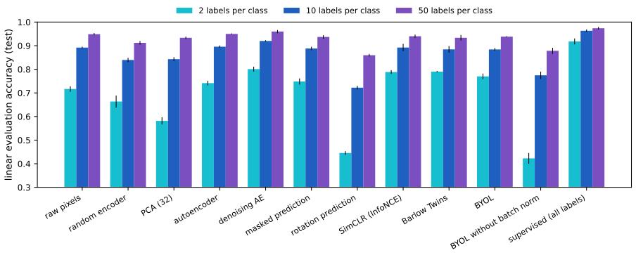
pp. 1063–1064 Another pretext task applies a transformation to the input and asks which transformation was used (Figure 32.4, a diagram, not reproduced). The reward is that it reuses the standard classification pipeline. The risk is a shortcut: trivial cues (chromatic aberration, matching pixels at patch borders) can solve the task without learning object structure, so the tasks add gaps between patches or colour jitter. Variants: relative position of two patches (an eight-way classification), jigsaw puzzles over a restricted set of permutations, and the prediction of one of four rotations (0, 90, 180, 270 degrees), the simplest and often the best of them. All have been overtaken by contrastive and masked methods. In our digits experiment rotation prediction is among the weakest pretext tasks (Figure 32.x.e): linear evaluation with 50 labels per class gives 0.86, below raw pixels (0.95); a plausible reason is that identifying a rotation of an 8×8 digit relies on the orientation of strokes, which does not separate 6 from 9 or 1 from 7 any better than pixels do.
32.3.4 Multiview representation learning
pp. 1064–1065 Multiview learning maps "similar" inputs, usually two views of one example, to nearby points and dissimilar inputs to distant ones. It needs (i) a supply of positive pairs, (ii) a mechanism that prevents all points from collapsing to one, and (iii) a loss combining an attraction of positive pairs with that mechanism. The family covers contrastive learning (positive and negative pairs), metric learning and non-contrastive learning (no negatives). Its strength is that prior knowledge about what should be close enters simply through the data, even across modalities. (Figure 32.5 draws the positive and negative pairs of SimCLR, CMC, SupCon and CLIP; it is a diagram and is not reproduced.)
32.3.4.1 View selection
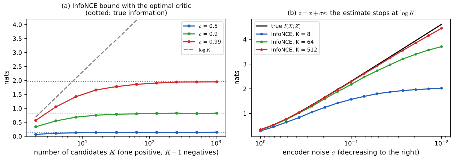
pp. 1065–1066 A training example is an anchor \(\bm x\), a positive \(\bm x^+\sim p^+(\bm x,\bm x^+)\) and negatives \(\bm x^-\sim p^-(\bm x^-\given\bm x)\); normally \(p^-\) ignores \(\bm x\) (an augmented view of another image). SimCLR forms \(\bm x=t(\bm x_0)\), \(\bm x^+=t'(\bm x_0)\) from two random augmentations (crops with flips, colour distortion, blur); SupCon takes as positives the examples with the same label; contrastive multiview coding splits an image into complementary channels (luma and chroma) with one encoder each; CLIP uses an image and its caption. Negatives are usually the other members of the minibatch; hard-negative mining picks negatives close to the anchor but costs a database of negatives, and reweighting within the batch captures part of the gain. Which views work best is the open question: Tian et al. argue for a "sweet spot" in the mutual information between the views, neither too small nor too large. The bound of gap 32.8 makes the first half of that statement precise: the contrastive loss cannot teach more than \(\MI(\text{view}_1;\text{view}_2)\) nats about the shared content, and if the views share nothing, for example because the augmentations are so strong that nothing survives, the loss stays at \(\log K\).
32.3.4.2 Contrastive losses
pp. 1066–1067 Given positives and negatives we look for an embedding \(f_\theta\) with \(f_\theta(\bm x)\) close to \(f_\theta(\bm x^+)\) and far from \(f_\theta(\bm x^-)\) (metric learning). The contrastive loss of Chopra, Hadsell and LeCun, as instantiated by Hadsell et al., pulls positives together and pushes negatives out to a distance \(\epsilon\): \[ \mathcal L_{\mathrm{contrastive}}=\E_{\bm x,\bm x^+,\bm x^-}\Big[\|f_\theta(\bm x)-f_\theta(\bm x^+)\|^2+\max\big(0,\epsilon-\|f_\theta(\bm x)-f_\theta(\bm x^-)\|^2\big)\Big], \tag{32.14} \] the triplet loss asks the positive to be closer than the negative by a margin \(\epsilon\) and gives no gradient once it is, \[ \mathcal L_{\mathrm{triplet}}=\E\Big[\max\big(0,\|f_\theta(\bm x)-f_\theta(\bm x^+)\|^2-\|f_\theta(\bm x)-f_\theta(\bm x^-)\|^2+\epsilon\big)\Big], \tag{32.15} \] and the InfoNCE (or multiclass \(N\)-pair) loss, with \(M\) negatives, avoids the margin altogether: \[ \mathcal L_{\mathrm{InfoNCE}}=-\E_{\bm x,\bm x^+,\bm x^-_{1:M}}\Bigg[\log\frac{\exp\big(f_\theta(\bm x)^\T g_\phi(\bm x^+)\big)}{\exp\big(f_\theta(\bm x)^\T g_\phi(\bm x^+)\big)+\sum_{i=1}^M\exp\big(f_\theta(\bm x)^\T g_\phi(\bm x_i^-)\big)}\Bigg]. \tag{32.16} \] Embeddings are normally \(\ell_2\)-normalised and the inner products divided by a temperature \(\tau\). The loss is a cross-entropy over \(K=M+1\) candidates, "which of these is the positive?", and the book relates it to mutual information, \[ \MI(X;Z)\ \ge\ \log M-\mathcal L_{\mathrm{InfoNCE}} . \tag{32.17} \]
Filling the gap 32.8: the bound (32.17), with \(K=M+1\) candidates, by classification p. 1067, (32.16)–(32.17)
Proof
Volume 1 proves the bound by a variational route (gap 19.5). Here is an independent argument that exposes the structure and the right constant. Take an anchor \(x\sim p(x)\), a candidate list of \(K\) points \(y_{1:K}\) in which a uniformly random position \(J\) holds a draw from \(p(y\given x)\) and every other position an independent draw from the marginal \(p(y)\). Write \(r(x,y)=p(y\given x)/p(y)\).
(i) InfoNCE is a classification loss. By Bayes' rule \(\Pr(J=j\given x,y_{1:K})\propto p(y_j\given x)\prod_{k\ne j}p(y_k)=\prod_kp(y_k)\,r(x,y_j)\), so the posterior of \(J\) is \(\operatorname{softmax}_j(\log r(x,y_j))\). For a critic \(f(x,y)\), the InfoNCE loss with the positive at position \(J\) is the cross-entropy \(L(f)=-\E\log\operatorname{softmax}_J\big(f(x,y_{1:K})\big)\) of the classifier \(\operatorname{softmax}(f)\) against the true law of \(J\). Cross-entropy equals entropy plus an expected KL divergence, so \[ L(f)=H(J\given x,y_{1:K})+\E\,\Dkl\big(\Pr(J\given x,y_{1:K})\,\|\,\operatorname{softmax}(f)\big)\ \ge\ H(J\given x,y_{1:K})=\log K-\MI(J;x,y_{1:K}), \] with equality iff \(f=\log r+c(x)\) (any function of \(x\) alone cancels in the softmax). Here \(H(J)=\log K\).
(ii) The information about the position is at most \(\MI(X;Y)\). The anchor \(x\) is independent of \(J\) (its marginal is \(p(x)\) for every \(J\)), so \(\MI(J;x,y_{1:K})=\MI(J;x)+\MI(J;y_{1:K}\given x)=\MI(J;y_{1:K}\given x)\). Fix \(x\). Given \(J=j\), \(y_{1:K}\) has law \(P_j=p(y_j\given x)\prod_{k\ne j}p(y_k)\), and mutual information is the mean KL divergence from the components to their mixture \(\bar P\). The mean KL divergence to any other distribution \(Q\) is larger (compensation identity: \(\frac1K\sum_j\Dkl(P_j\|Q)=\MI(J;y_{1:K}\given x)+\Dkl(\bar P\|Q)\)). Take \(Q=\prod_kp(y_k)\): then \(\Dkl(P_j\|Q)=\Dkl(p(y\given x)\|p(y))\) for every \(j\) (the factors for \(k\ne j\) cancel). Averaging over \(x\), \[ \MI(J;x,y_{1:K})\le\E_x\Dkl\big(p(y\given x)\|p(y)\big)=\MI(X;Y). \]
(iii) Conclusion. \(L(f)\ge\log K-\MI(J;x,y_{1:K})\ge\log K-\MI(X;Y)\), i.e. \(\MI(X;Y)\ge\log K-L(f)\) for every critic. Since \(L\ge0\), the estimate can never exceed \(\log K\). With \(M\) negatives \(K=M+1\), so the sharp form of (32.17) is \(\MI\ge\log(M+1)-\mathcal L_{\mathrm{InfoNCE}}\); the book's \(\log M\) is valid but weaker by \(\log(1+1/M)\). The bound is tight (as \(K\to\infty\)) for the optimal critic because \(\MI(J;x,y_{1:K})\to\MI(X;Y)\) (gap 19.5, remark (a)).
Numerical experiments. (a) In a finite example with a 3×3 joint distribution (\(\MI=0.0497\) nats) the exact optimal bound \(\log K-L^*\) is 0.0254, 0.0337 and 0.0378 for \(K=2,3,4\): below \(\MI\) and increasing in \(K\). (b) For a standard bivariate Gaussian pair with correlation \(\rho\) and the optimal critic \(\log r\), 60 000 anchors give, for \(\rho=0.9\) (\(\MI=0.830\)), 0.674 at \(K=8\) and 0.806 at \(K=64\); for \(\rho=0.99\) (\(\MI=1.959\)) 1.787 at \(K=32\); for \(\rho=0.5\) (\(\MI=0.144\)) 0.141 at \(K=512\) (Figure 32.x.d, (a)). A constant critic gives exactly \(\log K-L=0\).
Filling the gap 32.9: the gradient of InfoNCE, what the temperature does, and the limit to the triplet loss pp. 1066–1067, (32.15)–(32.16)
Proof
Gradient. Let \(s_0\) be the (temperature-scaled) similarity of the anchor with the positive and \(s_1,\dots,s_M\) with the negatives, \(L=-s_0+\log\sum_{k=0}^Me^{s_k}\). Then \(\partial L/\partial s_k=w_k-\mathbb 1[k=0]\) with the softmax weights \(w_k=e^{s_k}/\sum_je^{s_j}\) (confirmed by finite differences). With \(s_k=f(\bm x)^\T g(\bm y_k)/\tau\) the gradient on the anchor embedding is \[ \nabla_{f(\bm x)}L=\frac1\tau\Big(\sum_{k=0}^Mw_kg(\bm y_k)-g(\bm y_0)\Big)=\frac1\tau\big(\E_w[g]-g(\bm y_0)\big): \] the anchor is pulled toward the positive and pushed away from the \(w\)-weighted average of all candidates, so each negative is pushed with force proportional to its softmax weight. Negatives that already look unlike the anchor have exponentially small weight and contribute almost nothing (the soft counterpart of the triplet loss giving no gradient once satisfied), while the hardest negatives dominate.
Temperature. As \(\tau\to\infty\) all weights tend to \(1/K\) and the loss tends to \(\log K\) with a vanishing, undiscriminating gradient; as \(\tau\to0\) the weights concentrate on the largest \(s_k\). Precisely, with temperature-free similarities \(a_k=\tilde s_k-\tilde s_0\) (so that \(s_k-s_0=a_k/\tau\)), \[ \tau L_\tau=\tau\log\Big(1+\sum_{k\ge1}e^{a_k/\tau}\Big)\ \xrightarrow[\tau\to0]{}\ \max\big(0,\max_{k\ge1}a_k\big)=\max\big(0,\ s^{\mathrm{neg}}_{\max}-s^{\mathrm{pos}}\big), \] because \(\tau\log\sum_ke^{b_k/\tau}\to\max_kb_k\) (bounded between \(\max_kb_k\) and \(\max_kb_k+\tau\log K\)). So at small temperature InfoNCE becomes a hinge loss on the hardest negative with margin zero, which is the triplet loss (32.15) with \(\epsilon=0\) restricted to the hardest negative (confirmed: for negatives \((0.1,0.35,-0.2,0)\) and \(\tau=10^{-3}\), \(\tau L_\tau\) is \(2\times10^{-25}\) when the positive scores 0.4 and 0.0500 when it scores 0.3, the values \(\max(0,0.35-s^{\mathrm{pos}})\)). The difference from (32.15) at finite \(\tau\) is that the loss is smooth, never exactly zero and has no margin to tune.
The loss cannot reach zero for normalised embeddings. If \(f(\bm x),g(\bm y)\) have unit norm every inner product is in \([-1,1]\), so \(s_0\le1/\tau\) and \(s_k\ge-1/\tau\), and \(L\ge\log\big(1+M e^{-2/\tau}\big)\), with equality when the positive is identical to the anchor and every negative antipodal. For \(\tau=0.2\) and \(K=256\) this floor is 0.0113 (confirmed); the loss is then bounded away from zero by the geometry, which is why the learned embeddings never become infinitely separated.
32.3.4.3 Negative-free losses
pp. 1067–1068 Non-contrastive methods use only positive pairs and prevent collapse in other ways. Some add an explicit anti-collapse term: Barlow Twins drives the cross-correlation matrix \(C\) of the (batch-standardised) features of two views to the identity, \[ \mathcal L_{\mathrm{BT}}=\sum_{i=1}^p(1-C_{ii})^2+\lambda\sum_{i=1}^p\sum_{j\ne i}C_{ij}^2, \tag{32.18} \] and VICReg keeps the variance of each feature away from zero. Others have only an attractive term and rely on the dynamics of learning: BYOL and SimSiam minimise the squared distance between a predictor of the online representation and a target, \[ \mathcal L_{\mathrm{BYOL}}=\E_{\bm x,\bm x^+}\big[\|g_\phi(f_\theta(\bm x))-f_{\theta'}(\bm x^+)\|^2\big], \tag{32.19} \] with the target weights \(\theta'\) not receiving gradients: BYOL sets \(\theta'\) to an exponential moving average of \(\theta\), SimSiam copies \(\theta\) with a stop-gradient. DINO uses a cross-entropy between sharpened, batch-centred target outputs and the online outputs, \[ \mathcal L_{\mathrm{DINO}}=\E_{\bm x,\bm x^+}\big[H\big(f_{\theta'}(\bm x)/\tau,\ \operatorname{center}(f_\theta(\bm x^+))/\tau'\big)\big], \tag{32.20} \] and LeCun's joint-embedding predictive architecture (JEPA) generalises the squared distance to any notion of closeness in the embedding space. The common danger is collapse: the constant map makes every attraction term vanish.
Filling the gap 32.10: Barlow Twins: the minimum, why constant and redundant features are not optimal, and the link to CCA p. 1067, (32.18)
Proof
Let \(\hat A,\hat B\in\R^{n\times p}\) be the features of the two views standardised over the batch (zero mean, unit variance per column) and \(C=\hat A^\T\hat B/n\), so \(C_{ij}=\corr(\hat A_{:,i},\hat B_{:,j})\in[-1,1]\).
The minimum. \(\mathcal L_{\mathrm{BT}}\ge0\) and \(=0\) iff \(C=I\). Then \(C_{ii}=1\) means the \(i\)-th feature of both views is perfectly correlated, and, both being standardised, equal (equality in the Cauchy–Schwarz inequality), \(\hat A_{:,i}=\hat B_{:,i}\); and \(C_{ij}=0\) for \(i\ne j\) then says \(\corr(\hat A_{:,i},\hat A_{:,j})=0\): the features are decorrelated. So the optimum is a representation that is the same for both views and has an identity correlation matrix (whitened) on the batch. Check: two identical whitened views give \(\mathcal L_{\mathrm{BT}}=10^{-29}\).
Collapse is not a minimum. A constant feature has zero variance, so standardisation (or the variance term of VICReg) is undefined or penalised; the BT loss as a function of the correlation matrix cannot be lowered by constancy. A redundant representation, all \(p\) features equal, has \(C=\bm 1\bm 1^\T\) when the views agree, hence \(\mathcal L_{\mathrm{BT}}=\lambda p(p-1)\) (confirmed for \(p=6\), \(\lambda=0.1\): 3.0), strictly positive: the second term is what penalises dimensional collapse. Independent views give \(C\approx0\) and a loss of about \(p\) (5.9 for \(p=6\)), the cost of having no attraction.
Link to CCA. If each view's features are decorrelated (\(\hat A^\T\hat A/n=\hat B^\T\hat B/n=I\)), then \(Q=\hat A/\sqrt n\) and \(Q'=\hat B/\sqrt n\) have orthonormal columns and \(C=Q^\T Q'\), so the singular values of \(C\) are the canonical correlations \(\rho_i\) of the two views (confirmed). For \(\lambda=1\), \(\mathcal L_{\mathrm{BT}}=\Fn{C-I}^2=\Fn C^2-2\Tr C+p\ge\sum_i\rho_i^2-2\sum_i\rho_i+p=\sum_i(1-\rho_i)^2\), because \(\Tr C\le\|C\|_*=\sum\rho_i\); equality when \(C\) is symmetric positive semi-definite. So Barlow Twins on whitened features is a CCA-type objective, pushing all canonical correlations to 1, and its off-diagonal term is what enforces the whitening assumed by this reading. The kernel-independence (HSIC) connection mentioned by the book is of the same nature.
Filling the gap 32.11: BYOL and SimSiam in a one-mode linear model: a conserved quantity, the equilibrium and the collapse condition pp. 1067–1068, (32.19)
Proof
The book says that "the reasons why BYOL and SimSiam avoid collapse are not entirely clear" and cites a gradient-flow analysis of a linear model by Tian, Chen and Ganguli, who show that collapse can be avoided "given properly set hyperparameters". The following one-mode model is a deliberately small cousin of that analysis (my own simplification, not their theorem) in which everything can be computed.
Model. One direction of the data has variance \(s>0\); two views add independent noise of variance \(\sigma^2\): \(x_v=x+\sigma\varepsilon_v\), \(v=1,2\). Put \(a=\E x_1^2=s+\sigma^2\) and \(b=\E x_1x_2=s\), so \(a>b\) iff \(\sigma^2>0\). The online encoder is the scalar \(w\), the predictor the scalar \(p\), the target uses \(w\) with a stop-gradient. The loss is \(\mathcal L=\E(p\,w\,x_1-\sg(w)\,x_2)^2=w^2(p^2a-2pb+a)\) when the target is read at the same \(w\). The collapsed solution \(w=0\) has \(\mathcal L=0\), a global minimum.
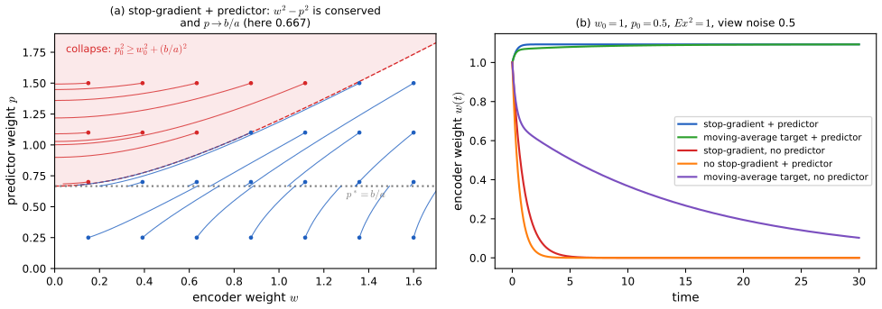
Gradient flow with stop-gradient and predictor (SimSiam). Differentiate only through the online branch: with \(e=pa-b\), \(\partial_w\mathcal L=2p\,w\,e\) and \(\partial_p\mathcal L=2w^2e\), so \[ \dot w=-2p\,w\,(pa-b),\qquad \dot p=-2w^2(pa-b). \] Then \(\tfrac{\d}{\d t}w^2=-4pw^2(pa-b)=\tfrac{\d}{\d t}p^2\), hence \(w^2-p^2\) is conserved. The fixed points are \(w=0\) (collapse, any \(p\)) and \(p=b/a\) (any \(w\)). For \(w\ne0\), \(p\) obeys \(\dot p=-2w^2a(p-b/a)\), so \(p\to b/a=s/(s+\sigma^2)<1\) (the predictor learns the shrinkage that predicts one view from the other), and \(w^2\to w_0^2-p_0^2+(b/a)^2\). This is possible only if the right side is positive: collapse happens iff \(p_0^2\ge w_0^2+(b/a)^2\) (if the quantity \(w_0^2-p_0^2+(b/a)^2\) is negative the flow reaches \(w=0\) at \(p=\sqrt{p_0^2-w_0^2}\); if it is zero it tends to \(w=0\) asymptotically). Confirmed: for \(s=1\), \(\sigma^2=0.5\) (\(b/a=0.6667\)), \(w_0=1\), \(p_0=0.5\) the flow ends at \(w=1.0929\), \(p=0.6667\) and \(w^2-p^2\) drifts by \(3\times10^{-10}\) over the whole run; the predicted collapse region agrees with simulation on all 64 starting points of an 8×8 grid (Figure 32.x.g, (a)). A predictor that is initially large compared with the encoder absorbs the signal and lets the encoder vanish; a predictor that is small does not.
Variants that collapse. (i) No predictor (\(p\equiv1\)): \(\dot w=-2w(a-b)=-2\sigma^2w\), so \(w(t)=w_0e^{-2\sigma^2t}\to0\): the views differ by their noise and the cheapest agreement is to output nothing (confirmed: \(e^{-10}\) at \(t=10\)). (ii) No stop-gradient: with the full gradient, \(\dot w=-2w(p^2a-2pb+a)\) and \(p^2a-2pb+a\ge a-b^2/a=\sigma^2(a+b)/a>0\), so \(w\to0\) at least exponentially for every \(p\). (iii) Moving-average target and no predictor: with target \(w'\), \(\dot w=-2(aw-bw')\), \(\dot w'=\eta(w-w')\), a linear system with matrix \(\begin{pmatrix}-2a&2b\\\eta&-\eta\end{pmatrix}\) of trace \(-(2a+\eta)\) and determinant \(2\eta(a-b)>0\), so both eigenvalues have negative real part: collapse, only more slowly. (iv) Moving-average target with a predictor (BYOL): the flow \(\dot w=-2pe'\), \(\dot p=-2we'\), \(\dot w'=\eta(w-w')\) with \(e'=pwa-w'b\) has the same fixed line \(w'=w\), \(p=b/a\); from \(w_0=1\), \(p_0=0.5\), \(\eta=0.2\) it ends at \(w=1.0925\), \(p=0.6661\) and does not collapse. The five variants are plotted in Figure 32.x.g, (b), and in the demonstration.
Limits. One mode only: with several data directions the predictor must align with the eigenbasis of the view covariance for the argument to go through, which is the content of the cited analysis; and real networks have normalisation layers, whose absence changed our digits experiment drastically (Figure 32.x.e: BYOL without batch normalisation in the projector and predictor reaches 0.42 with two labels per class against 0.77 with it).
Filling the gap 32.12: DINO: what centring and sharpening prevent p. 1068, (32.20)
Proof
For logits \(\bm S\) (online) and \(\bm T\) (target network) over \(K\) outputs and a batch of \(B\) inputs, let \(\bm q=\operatorname{softmax}\big((\bm T-\bar{\bm T})/\tau_t\big)\) with \(\bar{\bm T}\) the batch mean of the target logits ("center") and \(\bm p=\operatorname{softmax}(\bm S/\tau_s)\), and take \(\mathcal L=-\frac1B\sum_b\sum_kq_{bk}\log p_{bk}\). (The text of the book attaches the centring and the lower temperature \(\tau'<\tau\) to the target network; the printed (32.20) attaches them to the online argument, apparently by a slip of the subscripts; I follow the text.)
Collapse without centring. If every input gets the same output with a dominant coordinate, both \(\bm q\) and \(\bm p\) are (nearly) one-hot on the same class and \(\mathcal L\to0\), the global minimum: one-class collapse is optimal. (Numerically, for \(K=10\) and logits \(12\) on class 0: loss \(<10^{-6}\).)
Centring. If the target output is the same for every input, \(\bm T-\bar{\bm T}=0\), so \(\bm q\) is uniform and \(\mathcal L=H(\text{uniform},\bm p)=-\frac1K\sum_k\log p_k\ge\log K\) with equality iff \(\bm p\) is uniform (Jensen). Thus every constant-output state, including the one-hot collapse, has loss at least \(\log K\), while a balanced state, in which different inputs are assigned confidently to different classes with every class used equally often, is not penalised by centring: with logits \(12\) on class \(b\bmod K\) the centred target logits keep their argmax, \(\bm q\) is still one-hot to within \(e^{-\text{large}}\), \(\bm p\) matches it and \(\mathcal L<10^{-3}\) (here \(1.8\times10^{-126}\)). So centring removes one-class collapse by making it cost \(\ge\log K\), at the price of pushing the target toward the uniform distribution, since subtracting the mean flattens the dominant logit.
Sharpening. The uniform state is the other trivial state, and in it \(\mathcal L=\log K\) exactly (confirmed). Sharpening, the lower temperature \(\tau_t\), counteracts the flattening: the entropy of \(\bm q=\operatorname{softmax}(\bm z/\tau)\) is increasing in \(\tau\). With \(\beta=1/\tau\) and \(\log Z(\beta)=\log\sum_ke^{\beta z_k}\), \(H=\log Z-\beta\,\partial_\beta\log Z\), so \(\partial_\beta H=-\beta\,\partial^2_\beta\log Z=-\beta\operatorname{Var}_q(\bm z)\) and \(\partial_\tau H=\operatorname{Var}_q(\bm z)/\tau^3\ge0\). Lower \(\tau_t\) therefore lowers the entropy of the target (confirmed: the entropy is strictly decreasing along \(\tau=2,1,0.5,0.1\) for a random logit vector), which keeps the target away from uniform. The two devices act against opposite collapses and neither suffices alone, as the book says; whether this guarantees a non-trivial solution is a question about the dynamics, not about the loss, and has not been proved in general.
32.3.4.4 Tricks of the trade
pp. 1068–1069 Normalising the embeddings and using cosine similarity bounds the inner products in \([-1,1]\), after which a temperature \(\tau\) is needed (fixed or annealed; its effect is in gap 32.9). Contrastive losses with strong augmentation make the last layer too invariant for some tasks, so one either reads an earlier layer or inserts a projection head before the loss and discards it afterwards. Because the denominator of InfoNCE sums over negatives, large batches (4096 or more) are needed; MoCo keeps a queue of embeddings of earlier batches as extra negatives, with a momentum encoder (an exponential moving average of the online encoder) so that queued embeddings stay consistent, and an extra predictor, as in BYOL, removes the need for the queue. Vision transformers have replaced convolutional backbones in most recent work.
32.4 Theory of representation learning
p. 1069 Deep representation learning has displaced hand-designed features, but what these methods learn and what they guarantee is poorly understood. The book reviews three directions: identifiability (can the true latent factors be recovered?), information maximisation (does keeping information help?), and transfer bounds (the last of these is announced in the chapter's introduction but the text of this draft does not develop it).
32.4.1 Identifiability
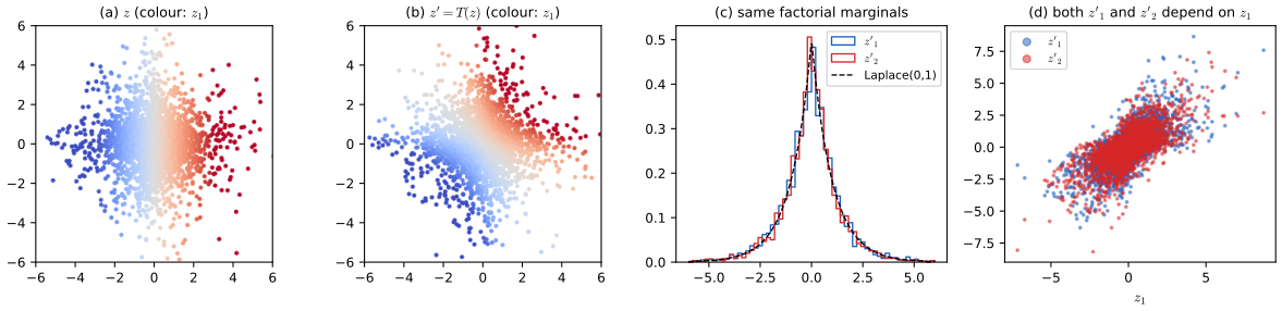
pp. 1069–1070 Assume the data are generated as \(\bm x=g(\bm z)\) with latents \(\bm z\sim p(\bm z)\) and a deterministic generator \(g\), and look for a representation \(\bm h=f_\theta(\bm x)\) that inverts it, \(\bm h=\bm z\). The model is identifiable if this is possible; since permutations and coordinate-wise reparametrisations \(h_i=f_i(z_{\pi(i)})\) are indistinguishable from the truth, theory aims at recovery up to those, and such a representation is called disentangled. Locatello et al. showed that, without extra assumptions on the data or the model, several popular methods cannot work: with a factorial prior \(p(\bm z)=\prod_ip_i(z_i)\) there is a bijection \(\bm z'=T(\bm z)\) that preserves the prior law and entangles all coordinates, and since it preserves the law of \(\bm z\) it preserves the law of the data, so the marginal likelihood cannot tell the two models apart; past successes came from tuning hyperparameters on supervised disentanglement scores. Additional information restores identifiability: auxiliary observations related to the latents through an exponential family (nonlinear ICA), data from several environments (causal representation learning), pairs of observations that differ in one latent factor, or a mixture prior (Kivva et al.).
Filling the gap 32.13: an explicit entangling bijection that preserves a factorial prior; why the data law cannot select the disentangled model pp. 1069–1070
Proof
Why a law-preserving \(T\) defeats identification. Suppose \(\bm z\sim p\) and \(\bm x=g(\bm z)\). If \(T\) is a bijection with \(T(\bm z)\sim p\), put \(\bm z'=T(\bm z)\) and \(g'=g\circ T^{-1}\). Then \(g'(\bm z')=g(\bm z)=\bm x\) and \(\bm z'\sim p\): the pair \((p,g')\) generates exactly the same law of \(\bm x\) as \((p,g)\), for the same prior, so no functional of the law of \(\bm x\) (the marginal likelihood included) separates them. If \(T\) makes every \(z'_i\) depend on every \(z_j\), then at most one of the two models can be disentangled with respect to the true factors.
Construction. Let \(F_i\) be the continuous, strictly increasing CDF of \(p_i\), \(\Phi\) the standard normal CDF, \(R\in SO(2)\) (or \(SO(d)\)) a rotation, and \[ T(\bm z)=F^{-1}\Big(\Phi\big(R\,\Phi^{-1}(F(\bm z))\big)\Big)\qquad(\text{coordinate-wise }F,\Phi). \] \(F_i(z_i)\) is uniform, so \(\bm\zeta=\Phi^{-1}(F(\bm z))\sim\N(0,I)\) has independent standard normal coordinates; \(R\bm\zeta\sim\N(0,I)\) by the rotation invariance of the standard normal density; \(\Phi(R\bm\zeta)\) has independent uniform coordinates and \(F^{-1}\) of these has independent coordinates with laws \(p_i\). So \(T(\bm z)\sim p\) and \(T\) is a bijection (a composition of bijections). Entanglement. By the chain rule, with \(\bm\zeta'=R\bm\zeta\), \(\bm z'=T(\bm z)\) and \(f_i=p_i\), \(\varphi=\Phi'\), \[ \frac{\partial z'_i}{\partial z_j}=\frac{\varphi(\zeta'_i)}{f_i(z'_i)}\ R_{ij}\ \frac{f_j(z_j)}{\varphi(\zeta_j)}, \] and both fractions are positive, so \(\partial z_i'/\partial z_j\ne0\) wherever \(R_{ij}\ne0\): for a rotation by 45 degrees every output coordinate depends on every input coordinate. (Confirmed by finite differences; and the map is measure preserving in the density form \(p(\bm z)=p(\bm z')|\det J|\), checked at two points.) Example. For a factorial Laplace prior in two dimensions and \(R\) the 45 degree rotation, \(40\,000\) transformed points have Laplace marginals (Kolmogorov–Smirnov \(p\)-values 0.80 and 0.30), their coordinates are independent (\(\operatorname{corr}(|z_1'|,|z_2'|)=0.0008\)), and yet \(|\operatorname{corr}(z_2',z_1)|\) and \(|\operatorname{corr}(z_1',z_1)|\) both exceed 0.3 (Figure 32.x.f).
The linear case is different. A linear rotation of the Gaussian prior is already law preserving (rotation invariance), which is why factor analysis latents are identified only up to a rotation. For a non-Gaussian factorial prior a linear rotation changes the law: for the Laplace prior and the 45 degree rotation \(\operatorname{corr}(|z_1|,|z_2|)=0.43\) after rotating, so the rotated coordinates are no longer independent and linear independent component analysis can find the unmixing up to permutation and scale, provided at most one source is Gaussian (the Darmois–Skitovich theorem, used by Comon (1994); Section 28.6.2). Non-identifiability is therefore a statement about nonlinear generators with a prior that admits law-preserving nonlinear maps (any factorial prior with continuous marginals does, as above); linear ICA escapes it only because the rotation of non-Gaussian sources is not law preserving.
See also: the ICA rotation demonstration (this volume) for the identifiable linear case, and unmixing demonstration (deep-learning course).
32.4.2 Information maximization
pp. 1070–1071 A natural desideratum is to lose as little information about the input as possible (the InfoMax principle of Linsker and of Bell and Sejnowski). But information theory does not say which bits matter, and for artificial networks there is a trivial solution that biological systems do not have: copy the input. Constraints (architecture, optimisation) or side information (labels) must say which bits to keep. The information bottleneck (Section 5.6.1) uses a second variable \(Y\) to say which bits matter, and trades compression against prediction, \[ \operatorname*{maximise}_\theta\ \ \MI(Z;Y)-\beta\,\MI(X;Z), \tag{32.21} \] whose self-consistent solution and variational version (VIB) are derived in gap 5.23 and Section 5.6.2; Figure 32.1 above was produced with a VIB. Many recent InfoMax-motivated methods (CPC, deep InfoMax) have no compression term; they maximise a lower bound of information subject to architectural constraints. The difficulty is that most learned encoders are deterministic maps from continuous inputs to continuous representations, and then the true information is infinite and all estimators are weak lower bounds; Tschannen et al. showed that for invertible networks, whose true information is infinite throughout training, maximising an estimator still gives useful features, so the success of these methods may owe more to the geometry and bias of the estimators than to information itself.
Filling the gap 32.14: infinite information of deterministic encoders, the ceiling of estimators, and the trivial InfoMax solution pp. 1070–1071
Proof
InfoMax alone is satisfied by the identity. By the data-processing inequality \(\MI(X;Z)\le\MI(X;X)\) for any \(Z\) that is a (possibly random) function of \(X\), so \(Z=X\), or any injective function of \(X\), maximises \(\MI(X;Z)\) (the value is \(H(X)\) for a discrete \(X\)).
Continuous input and an injective deterministic encoder: \(\MI=+\infty\). Let \(X\) have a density and \(Z=f(X)\) with \(f\) injective and measurable. Let \(q_m(X)\) be the index of the cell of a partition of the input space into \(m\) cells of equal probability. Since \(q_m(X)\) is a function of \(Z\) (\(f\) is injective, so \(Z\) determines \(X\)), \(\MI(X;Z)\ge\MI(q_m(X);Z)=H(q_m(X))=\log m\to\infty\). The same computation is visible for a one-dimensional normal: quantised into \(4,16,64,256\) equal-probability cells the information is \(1.386,2.773,4.159,5.545\) nats \(=\log m\) (confirmed). A mutual information that is infinite throughout training carries no signal about the quality of the representation. A sharper picture is given by adding noise: for \(x\sim\N(0,1)\) and \(z=x+\sigma\varepsilon\), \[ \MI(X;Z)=\tfrac12\log\big(1+\sigma^{-2}\big)\ \xrightarrow[\sigma\to0]{}\ \infty, \] the Gaussian channel formula (Chapter 5): \(0.805\) nats at \(\sigma=0.5\), \(2.31\) at \(\sigma=0.1\) and \(4.61\) at \(\sigma=0.01\).
Estimators saturate. Any estimate of the form \(\log K-L\) with \(L\ge0\) (InfoNCE, gap 32.8) is at most \(\log K\), whatever the true information. Distribution-free lower bounds from \(N\) samples cannot certify more than order \(\log N\) either (McAllester and Stratos, 2020), so in the regime of large information the estimators are weak, as the book says. In the noisy-encoder example the estimate with the optimal critic tracks the truth up to \(\log K\) and then flattens: at \(K=2048\) it is 0.792 against 0.805 for \(\sigma=0.5\) and 2.293 against 2.308 for \(\sigma=0.1\), while for \(\sigma=0.01\) with only \(K=64\) candidates it remains below \(\log64=4.16\) although the truth is 4.61 (Figure 32.x.d, (b)).
p. 1071 Some work learns stochastic representations whose information is constrained (the variational bottleneck of Alemi et al.), and Fischer and Alemi show a gain in robustness, but scaling up models and data with deterministic representations still gives the best results; whether constraining information helps general representations is open.
S32 Supplement supplement
The online supplement's Chapter 32 (pages 301–302) consists of the chapter title only; there is no material to cover.
Practice problems
The book has no end-of-chapter exercises for Chapter 32, so here are three short problems of my own, with complete solutions (hidden).
Practice problem 32.1 (CKA and CCA by hand). Four examples have the two-neuron representation \(X\) with rows \((1,0),(-1,0),(0,1),(0,-1)\) and \(Y=X\operatorname{diag}(1,3)\). (a) Compute linear CKA of \(X\) and \(Y\). (b) Compute the canonical correlations and \(R^2_{\mathrm{CCA}}\), \(R^2_{\mathrm{LR}}\). (c) What is the CKA of \(X\) and \(X\) rotated by 90 degrees? (d) Check (a) with the formula (32.12).
Solution
Both matrices are already centred (each column sums to 0). (a) \(X^\T Y=\operatorname{diag}(2,6)\), \(\Fn{X^\T Y}^2=4+36=40\); \(X^\T X=\operatorname{diag}(2,2)\), \(\Fn{X^\T X}=\sqrt8\); \(Y^\T Y=\operatorname{diag}(2,18)\), \(\Fn{Y^\T Y}=\sqrt{4+324}=\sqrt{328}\). By (32.2), \(\mathrm{CKA}=40/\sqrt{8\cdot328}=40/\sqrt{2624}=0.7809\). (b) \(Y=XD\) with \(D\) invertible, so the column spaces coincide and both canonical correlations are 1 (gap 32.3): \(R^2_{\mathrm{CCA}}=\bar\rho=1\); the regression of \(Y\) on \(X\) is exact, so \(R^2_{\mathrm{LR}}=1\) (gap 32.5, equal ranks). CKA is less than 1 because \(D\) is not orthogonal (gap 32.2). (c) \(X\to XR\) with \(R\) orthogonal leaves \(XX^\T\) unchanged, so CKA \(=1\). (d) The principal components of \(X\) and \(Y\) are the same two unit vectors in the same order, so \((\bm u_i^\T\bm u'_j)^2=\delta_{ij}\); with \(\lambda=(2,2)\), \(\lambda'=(2,18)\) the numerator of (32.12) is \(2\cdot2+2\cdot18=40\) and the denominator \(\sqrt{4+4}\sqrt{4+324}\), the same value. (Confirmed numerically.)
Practice problem 32.2 (what InfoNCE can certify). (a) A critic is constant. What are the InfoNCE loss and the bound with \(K\) candidates? (b) How many candidates are needed to certify \(\MI(X;Y)=3\) nats? (c) For unit-norm embeddings what is the smallest possible loss for \(\tau=0.1\), \(K=128\), and for \(\tau=0.2\), \(K=256\)?
Solution
(a) All scores are equal, so the softmax is uniform and \(L=\log K\); the bound \(\log K-L=0\). (b) The bound never exceeds \(\log K\) (gap 32.8), so certifying 3 nats needs \(\log K>3\), i.e. \(K>e^3=20.09\), so \(K\ge21\) candidates (20 negatives); and since a finite \(K\) is never tight, in practice more (for \(\rho=0.99\), where \(\MI=1.96\) and \(e^{\MI}=7.1\), the estimate needed \(K=512\) to come within 0.02, Figure 32.x.d). (c) The floor is \(\log(1+(K-1)e^{-2/\tau})\) (gap 32.9): \(\log(1+127e^{-20})=2.6\times10^{-7}\) for \(\tau=0.1\), \(K=128\), and \(\log(1+255e^{-10})=0.0113\) for \(\tau=0.2\), \(K=256\). The loss therefore cannot be driven to zero when the embeddings are normalised and the temperature is not tiny.
Practice problem 32.3 (the one-mode SimSiam model). Take signal variance \(s=1\) and view-noise variance \(\sigma^2=3\), stop-gradient with predictor, initial weights \(w_0=0.8\), \(p_0=0.3\). (a) Find \(a\), \(b\), the limiting predictor and encoder. (b) For which \(p_0\) (with \(w_0=0.8\)) does the encoder collapse? (c) Without the predictor, how fast does \(w\) decay and what is \(w(1)\)?
Solution
(a) \(a=s+\sigma^2=4\), \(b=s=1\), so \(p\to b/a=0.25\); the conserved quantity is \(w_0^2-p_0^2=0.64-0.09=0.55\), so \(w^2\to0.55+0.0625=0.6125\) and \(w\to0.7826\) (gap 32.11; simulation gives 0.7826 and 0.2500). (b) Collapse iff \(p_0^2\ge w_0^2+(b/a)^2=0.64+0.0625=0.7025\), i.e. \(p_0\ge0.8382\). (c) With \(p\equiv1\), \(\dot w=-2\sigma^2w=-6w\), so \(w(t)=0.8\,e^{-6t}\) and \(w(1)=0.8e^{-6}=0.00198\).
Demonstrations
- Comparing two representations: CKA and CCA (Section 32.2.2): six similarity indexes of a representation and a transformed noisy copy or unrelated data, as the number of examples and neurons, the noise and the transformation change.
- The InfoNCE bound, negatives and temperature (Section 32.3.4.2): the estimate against the number of candidates and the true information, and the softmax weights of the gradient.
- Why BYOL and SimSiam need not collapse (Section 32.3.4.3): the one-mode flow for five variants, with its conserved quantity and collapse region.
Python code for every figure: code index. Data used by the demonstrations: data/ch32-reps.json (the representation tables of the first demonstration), data/ch32-infonce.json (the draws of the second); the third computes everything in the page. Companion demos: Volume 1 and the deep-learning course.
Notes on the book
Points where the book is imprecise or wrong
- After (32.8), the condition for (32.9). The text says the variance-weighted CCA index (32.8) equals the regression \(R^2\) (32.9) "when \(p_2\ge p_1\)". The identity holds exactly when \(\rank\tilde Y\le\rank\tilde X\), the opposite direction (gap 32.5): with an 8-neuron \(X\) and a 20-neuron \(Y\) the two are 0.154 and 0.065, and with a 20-neuron \(X\) and an 8-neuron \(Y\) both are 0.184.
- (32.10). The mean squared canonical correlation is divided by \(p_1\); the definition (32.4) divides by \(p=\min(\rank X,\rank Y)\), which equals \(p_1\) only for \(p_1\le p_2\) with full-rank representations.
- (32.17). With \(M\) negatives the InfoNCE bound is \(\MI\ge\log(M+1)-\mathcal L_{\mathrm{InfoNCE}}\), because there are \(K=M+1\) candidates (gap 32.8). The printed \(\log M\) is true but weaker.
- Section 32.3.4, paragraph after Figure 32.5. "They all involve a repulsion component that pulls positive pairs closer together": the component that pulls positive pairs together is an attraction; repulsion pushes negatives apart.
- Section 32.3.4.1. "negative examples are selected by randomly choosing \(x^+\) from other elements in a minibatch" should read \(x^-\).
- (32.20). The text says the centring and the lower temperature \(\tau'<\tau\) are applied to the target network, but the printed formula attaches both to the online network \(f_\theta(\bm x^+)\) and the plain temperature to the target \(f_{\theta'}(\bm x)\) (gap 32.12).
- Section 32.3.2.3. "the resulting linear autoencoder model can learn the principal components": the minimisers of (32.13) learn the principal subspace; the weights are determined only up to an invertible matrix and need not be the principal components (gap 32.6).
- Section 32.2.2.2, curse of dimensionality. The condition "more neurons than examples" can be weakened to \(n-1\) linearly independent neurons in one of the representations, because centring removes one dimension, and nothing is needed of the other (gap 32.3).
- Introduction and Section 32.4. The introduction announces "transfer bounds" as the third part of the theory, but Section 32.4 treats only identifiability and information maximisation.
References
- Alemi, A. A., Fischer, I., Dillon, J. V. and Murphy, K. (2017). Deep variational information bottleneck. International Conference on Learning Representations.
- Björck, A. and Golub, G. H. (1973). Numerical methods for computing angles between linear subspaces. Mathematics of Computation, 27(123), 579–594.
- Caron, M., Touvron, H., Misra, I., Jégou, H., Mairal, J., Bojanowski, P. and Joulin, A. (2021). Emerging properties in self-supervised vision transformers. IEEE/CVF International Conference on Computer Vision.
- Chen, T., Kornblith, S., Norouzi, M. and Hinton, G. (2020). A simple framework for contrastive learning of visual representations. International Conference on Machine Learning.
- Chen, X. and He, K. (2021). Exploring simple Siamese representation learning. IEEE/CVF Conference on Computer Vision and Pattern Recognition.
- Comon, P. (1994). Independent component analysis, a new concept? Signal Processing, 36(3), 287–314.
- Eckart, C. and Young, G. (1936). The approximation of one matrix by another of lower rank. Psychometrika, 1(3), 211–218.
- Grill, J.-B. et al. (2020). Bootstrap your own latent: a new approach to self-supervised learning. Advances in Neural Information Processing Systems, 33.
- He, K., Chen, X., Xie, S., Li, Y., Dollár, P. and Girshick, R. (2022). Masked autoencoders are scalable vision learners. IEEE/CVF Conference on Computer Vision and Pattern Recognition.
- Kornblith, S., Norouzi, M., Lee, H. and Hinton, G. (2019). Similarity of neural network representations revisited. International Conference on Machine Learning.
- Locatello, F. et al. (2019). Challenging common assumptions in the unsupervised learning of disentangled representations. International Conference on Machine Learning.
- McAllester, D. and Stratos, K. (2020). Formal limitations on the measurement of mutual information. International Conference on Artificial Intelligence and Statistics.
- Morcos, A. S., Raghu, M. and Bengio, S. (2018). Insights on representational similarity in neural networks with canonical correlation. Advances in Neural Information Processing Systems, 31.
- Murphy, K. P. (2023). Probabilistic Machine Learning: Advanced Topics. MIT Press (December 2025 online draft).
- van den Oord, A., Li, Y. and Vinyals, O. (2018). Representation learning with contrastive predictive coding. arXiv:1807.03748.
- Poole, B., Ozair, S., van den Oord, A., Alemi, A. and Tucker, G. (2019). On variational bounds of mutual information. International Conference on Machine Learning.
- Raghu, M., Gilmer, J., Yosinski, J. and Sohl-Dickstein, J. (2017). SVCCA: singular vector canonical correlation analysis for deep learning dynamics and interpretability. Advances in Neural Information Processing Systems, 30.
- Robert, P. and Escoufier, Y. (1976). A unifying tool for linear multivariate statistical methods: the RV-coefficient. Journal of the Royal Statistical Society C, 25(3), 257–265.
- Tian, Y., Chen, X. and Ganguli, S. (2021). Understanding self-supervised learning dynamics without contrastive pairs. International Conference on Machine Learning.
- Tishby, N., Pereira, F. C. and Bialek, W. (2000). The information bottleneck method. arXiv:physics/0004057.
- Tschannen, M., Djolonga, J., Rubenstein, P. K., Gelly, S. and Lucic, M. (2020). On mutual information maximization for representation learning. International Conference on Learning Representations.
- Vincent, P., Larochelle, H., Bengio, Y. and Manzagol, P.-A. (2008). Extracting and composing robust features with denoising autoencoders. International Conference on Machine Learning.
- Zbontar, J., Jing, L., Misra, I., LeCun, Y. and Deny, S. (2021). Barlow Twins: self-supervised learning via redundancy reduction. International Conference on Machine Learning.
The numerical statements in the text (the identity (32.2) and the range and invariances of CKA; the CCA algorithm, its invariances, the rank and expected-overlap formulas and the saturation at \(n-1\) neurons; the SVCCA, PWCCA and \(R^2_{\mathrm{LR}}\) properties and the identities (32.9)–(32.12) with the corrected condition; the basis dependence of ridge regression; the linear autoencoder optimum and subspace, the linear denoiser gains and Gaussian masked prediction; the InfoNCE bound, its gradient, its zero-temperature limit and its floor for unit vectors; Barlow Twins, DINO and the one-mode BYOL model with its conserved quantity and collapse region; the entangling map and its Jacobian; the Gaussian channel and the estimator ceiling; the worked practice problems and the trained-network numbers) were confirmed numerically.