Optimization
Fitting a model means minimising a loss. This chapter is a toolbox of solvers and of the theory that says when they work. It starts with what a minimum is (optimality conditions, convexity, smoothness, subgradients), then moves through first-order methods (gradient descent, line search, momentum), second-order methods (Newton, BFGS, trust regions) and the stochastic methods that dominate machine learning (SGD, learning-rate schedules, averaging, variance reduction, adaptive steps). It then adds constraints (Lagrange multipliers, KKT, linear and quadratic programs), non-smooth regularisers (proximal methods) and bound optimisation, whose most famous instance is the EM algorithm. The notes prove the convergence rates and characterisations the book quotes.
Ch. 1 Introduction Ch. 2 Univariate probability Ch. 3 Multivariate probability Ch. 4 Statistics Ch. 5 Decision theory Ch. 6 Information theory Ch. 7 Linear algebra Ch. 8 Optimisation Ch. 9 Discriminant analysis Ch. 10 Logistic regression Ch. 11 Linear regression Ch. 12 GLMs Ch. 13 Networks for tabular data Ch. 14 Networks for images Ch. 15 Networks for sequences Ch. 16 Exemplar-based methods Ch. 17 Kernel methods Ch. 18 Trees and boosting Ch. 19 Fewer labels Ch. 20 Dimensionality reduction Ch. 21 Clustering Ch. 22 Recommender systems Ch. 23 Graph embeddings
How to read these notes
They follow the book. Sections carry the book's numbers (8.2.3, 8.4.6.3, ...) and equations the book numbers keep their numbers, e.g. \((8.29)\); equations without a number are steps the book skips. Sections 8.4.5, 8.5.5, 8.6 and 8.7 are starred (optional) in the book; they are covered here because the later chapters (lasso, SVMs, mixtures) rely on them.
Filling the gaps. Wherever the book writes "one can show", quotes a rate from the literature or skips a step, an orange Filling the gap box (or a Result box with its proof) gives the full argument. Proofs start hidden: open one with its bar, or use the buttons below.
Notation. The loss is \(\cL(\bth)\) with gradient \(\bm g(\bth)=\nabla\cL(\bth)\) and Hessian \(\bm H(\bth)=\nabla^2\cL(\bth)\); \(\bth^*\) is a minimiser and \(\cL^*=\cL(\bth^*)\). The plain letter \(L\) is a Lipschitz constant of the gradient and \(m\) a strong-convexity constant, with condition number \(\kappa=L/m\). \(\|\cdot\|\) is the Euclidean norm.
Figures and demonstrations. Every computed figure is reproduced by the Python code, and the book's illustrations are redrawn from computed examples; two hand-drawn sketches (Figures 8.3 and 8.13) are not reproduced. Data: simulated points for LMS (Figure 8.16), a small MNIST network instead of FashionMNIST (Figure 8.17), the galaxy velocities of Roeder (1990) as the density of Figure 8.24, and Old Faithful for EM (Figure 8.25), as stated in the captions. Six supplementary figures (8.S1–8.S6) illustrate the filled gaps. The ▶ Demo boxes open an interactive demonstration set to the case being discussed.
Main reference
K. P. Murphy, Probabilistic Machine Learning: An Introduction, MIT Press (2022), Chapter 8, pages 275–320 (book page: probml.github.io/pml-book/book1.html). Section, equation, figure and exercise numbers below refer to this book. The explanations, derivations, figures and code are my own.
Companion courses
Parts of this chapter are developed, in other notation, elsewhere on this site. Where a result is proved in full there, these notes give the statement and a short sketch and link to it.
- Foundations of Deep Learning (Bishop and Bishop): 7.1 error surfaces, 7.2 gradient descent and SGD, 7.3.1 momentum, 7.3.2 learning-rate schedules, 7.3.3 RMSProp and Adam, Appendix C.1 Lagrange multipliers, C.2 the KKT conditions, 15.3 EM, 15.4 the evidence lower bound.
- Bayesian and Probabilistic Machine Learning (Bishop): 5.2.2 local quadratic approximation, 5.2.4 gradient descent optimisation, 9.2.2 EM for Gaussian mixtures, 9.4 the EM algorithm in general.
- The Elements of Statistical Learning: 3.4.2 the lasso, 3.8.6 pathwise coordinate optimisation, 8.5 the EM algorithm.
What this chapter adds: the convexity toolkit (strong convexity, conjugates, subgradients), convergence rates with proofs (exact line search, gradient descent, Newton, heavy ball, accelerated and proximal methods), quasi-Newton and trust-region methods, variance-reduced SGD, the failure of Adam and its repairs, linear and quadratic programming, proximal operators (including quantisation) and MM algorithms beyond EM.
The chapter at a glance
- 8.1 Optimality conditions (Result 8.1); convex functions, the Hessian test and strong convexity (Results 8.2–8.3); smoothness and the descent lemma (Result 8.4); subgradients.
- 8.2 Gradient descent: the step-size bound (Result 8.5), exact line search and the Kantorovich rate (Result 8.6), the \(O(1/t)\) and linear rates (Result 8.7), heavy ball and Nesterov momentum.
- 8.3 Newton's method and its quadratic convergence (Result 8.8), BFGS (Result 8.9), trust regions (Result 8.10).
- 8.4 SGD: minibatch variance, convergence and the Robbins–Monro conditions (Result 8.11), averaging, SVRG and SAGA, AdaGrad, RMSProp, Adam, and why Adam can fail.
- 8.5 Lagrange multipliers (Result 8.12), KKT conditions (Result 8.13), linear and quadratic programs.
- 8.6 Proximal operators, projected and proximal gradient, ISTA and FISTA rates (Result 8.15).
- 8.7 MM algorithms, EM, EM for Gaussian mixtures with MLE and MAP updates.
Prerequisites. Multivariate calculus (gradients, Hessians, Taylor's theorem), the linear algebra of Chapter 7 (eigenvalues, positive definite matrices), and the likelihood and KL divergence of Chapters 4 and 6.
8.1 Introduction
p. 275 Parameter estimation is the optimisation problem \[ \bth^*\in\argmin_{\bth\in\Theta}\cL(\bth), \tag{8.1} \] with \(\Theta\subseteq\R^D\) (continuous optimisation). Maximising a reward \(R\) is minimising \(-R\). An algorithm that solves (8.1) is a solver.
8.1.1 Local vs global optimization
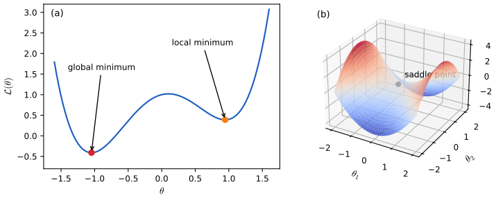
pp. 275–276 A point satisfying (8.1) is a global optimum; finding one is intractable in general. \(\bth^*\) is a local minimum if \(\cL(\bth^*)\le\cL(\bth)\) for all \(\bth\) within some distance \(\delta>0\) (8.2), and a strict local minimum if the inequality is strict for \(\bth\ne\bth^*\) (8.3). A method that converges to a stationary point from any start is called globally convergent, which says nothing about reaching a global minimum.
8.1.1.1 Optimality conditions for local vs global optima
Result 8.1 (first- and second-order optimality conditions) pp. 276–277
Let \(\cL\) be twice continuously differentiable on an open set containing \(\bth^*\), with \(\bm g^*=\nabla\cL(\bth^*)\) and \(\bm H^*=\nabla^2\cL(\bth^*)\).
- Necessary. If \(\bth^*\) is a local minimum then \(\bm g^*=\bm 0\) and \(\bm H^*\succeq0\).
- Sufficient. If \(\bm g^*=\bm 0\) and \(\bm H^*\succ0\) then \(\bth^*\) is a strict local minimum.
Neither condition is both: \(\cL=\theta_1^2+\theta_2^3\) has \(\bm g^*=\bm 0\) and \(\bm H^*=\diag(2,0)\succeq0\) at the origin, which is not a minimum; \(\cL=\theta^4\) has a strict minimum with \(\bm H^*=0\).
Proof
Gradient. Fix a direction \(\bm d\) and set \(\varphi(\eta)=\cL(\bth^*+\eta\bm d)\). It has a local minimum at \(\eta=0\), so \(\varphi'(0)=\bm d^\T\bm g^*=0\). As this holds for every \(\bm d\) (take \(\bm d=\bm g^*\)), \(\bm g^*=\bm 0\).
Hessian. By Taylor's theorem with \(\bm g^*=\bm 0\), \(\varphi(\eta)=\varphi(0)+\tfrac12\eta^2\bm d^\T\bm H^*\bm d+o(\eta^2)\). If \(\bm d^\T\bm H^*\bm d<0\) for some \(\bm d\), then \(\varphi(\eta)<\varphi(0)\) for all small \(\eta\ne0\), contradicting minimality. So \(\bm H^*\succeq0\).
Sufficiency. Let \(\lambda_0>0\) be the smallest eigenvalue of \(\bm H^*\). By continuity of the Hessian there is a ball \(B\) around \(\bth^*\) on which every \(\nabla^2\cL(\bm\xi)\) has smallest eigenvalue at least \(\lambda_0/2\). For \(\bth\in B\), the mean-value form of Taylor's theorem gives a point \(\bm\xi\) on the segment from \(\bth^*\) to \(\bth\) with \[ \cL(\bth)=\cL(\bth^*)+\tfrac12(\bth-\bth^*)^\T\nabla^2\cL(\bm\xi)(\bth-\bth^*)\ge\cL(\bth^*)+\tfrac{\lambda_0}{4}\|\bth-\bth^*\|^2, \] which is larger than \(\cL(\bth^*)\) for \(\bth\ne\bth^*\). \(\square\)
Saddles. If \(\bm H^*\) has eigenvalues of both signs, the eigenvectors give directions of increase and of decrease, so the stationary point is a saddle. The converse fails: in the example \(\theta_1^2+\theta_2^3\) above the origin is a saddle (the function changes sign along \(\theta_2\)) although \(\bm H^*\) has no negative eigenvalue. For non-smooth convex functions the first-order condition becomes \(\bm 0\in\partial\cL(\bth^*)\) (Filling the gap 8.3).
8.1.2 Constrained vs unconstrained optimization
p. 277 Constraints split into inequalities \(g_j(\bth)\le0\), \(j\in\mathcal I\), and equalities \(h_k(\bth)=0\), \(k\in\mathcal E\); the feasible set is \[ \mathcal C=\{\bth:g_j(\bth)\le0,\ j\in\mathcal I,\ h_k(\bth)=0,\ k\in\mathcal E\}\subseteq\R^D, \tag{8.4} \] and the problem is \(\argmin_{\bth\in\mathcal C}\cL(\bth)\) (8.5). Constraints can create optima (Figure 8.2) or make \(\mathcal C\) empty (an infeasible problem). Penalty terms and the Lagrangian (Section 8.5) turn constraints into objective terms.
8.1.3 Convex vs nonconvex optimization
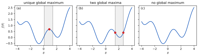
pp. 277–281 A set \(\mathcal S\) is convex if \(\lambda\bm x+(1-\lambda)\bm x'\in\mathcal S\) for all \(\bm x,\bm x'\in\mathcal S\), \(\lambda\in[0,1]\) (8.6) (Figure 8.3 of the book, a hand-drawn gallery of shapes, is not reproduced). A function on a convex set is convex if \[ f(\lambda\bm x+(1-\lambda)\bm y)\le\lambda f(\bm x)+(1-\lambda)f(\bm y),\qquad\lambda\in[0,1], \tag{8.7} \] equivalently if its epigraph \(\epi f=\{(\bm x,t):t\ge f(\bm x)\}\) is a convex set; strictly convex if the inequality is strict for \(\bm x\ne\bm y\), \(\lambda\in(0,1)\); (strictly) concave if \(-f\) is (strictly) convex.
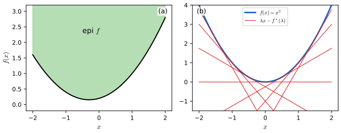
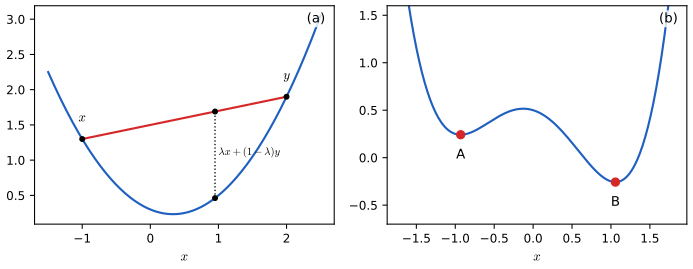
Filling the gap 8.1: why convexity makes every local minimum global, and the six examples pp. 277–279
Derivation
Local is global. Let \(\cL\) be convex on the convex set \(\mathcal C\) and \(\bth^*\) a local minimiser. If some \(\bth'\in\mathcal C\) had \(\cL(\bth')<\cL(\bth^*)\), the points \(\bth_\lambda=\bth^*+\lambda(\bth'-\bth^*)\in\mathcal C\) would satisfy \(\cL(\bth_\lambda)\le(1-\lambda)\cL(\bth^*)+\lambda\cL(\bth')<\cL(\bth^*)\) for every \(\lambda\in(0,1]\), and \(\bth_\lambda\to\bth^*\) as \(\lambda\to0\): no neighbourhood of \(\bth^*\) would be free of better points. The same inequality shows that the set of minimisers is convex, and a strictly convex function has at most one minimiser (the midpoint of two would be strictly better).
Epigraph. If (8.7) holds and \((\bm x,s),(\bm y,t)\in\epi f\) then \(f(\lambda\bm x+(1-\lambda)\bm y)\le\lambda s+(1-\lambda)t\), so the mixture is in the epigraph. Conversely, applying epigraph convexity to \((\bm x,f(\bm x))\) and \((\bm y,f(\bm y))\) gives (8.7).
The examples on p. 279. On their domains the second derivatives are \((x^2)''=2\), \((e^{ax})''=a^2e^{ax}\), \((-\log x)''=x^{-2}\), \((x^a)''=a(a-1)x^{a-2}\ge0\) for \(a\ge1\) (also for \(a\le0\)), \((x\log x)''=1/x\), all non-negative, so Result 8.2 applies. \(|x|^a\) with \(a\ge1\) is not twice differentiable at 0; it is the composition of the convex non-decreasing \(t\mapsto t^a\) on \([0,\infty)\) with the convex \(|x|\), and such a composition is convex: \[|\lambda x+(1-\lambda)y|^a\le(\lambda|x|+(1-\lambda)|y|)^a\le\lambda|x|^a+(1-\lambda)|y|^a. \] \(\square\)
8.1.3.3 Characterization of convex functions
Result 8.2 (Theorem 8.1.1: the first-order and Hessian tests) p. 280
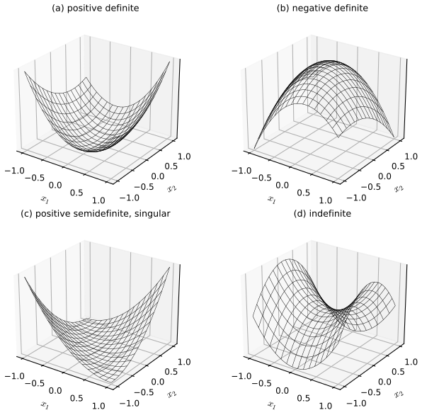
Let \(f\) be differentiable on an open convex set \(\mathcal S\). (a) \(f\) is convex iff \(f(\bm y)\ge f(\bm x)+\nabla f(\bm x)^\T(\bm y-\bm x)\) for all \(\bm x,\bm y\in\mathcal S\). (b) If \(f\) is twice differentiable, \(f\) is convex iff \(\nabla^2f(\bm x)\succeq0\) for all \(\bm x\in\mathcal S\); and \(\nabla^2f\succ0\) everywhere implies strict convexity (not conversely: \(x^4\)). In particular the quadratic form \(\bm x^\T\bm A\bm x\) (8.8), with Hessian \(2\bm A\) for symmetric \(\bm A\), is convex iff \(\bm A\succeq0\), strictly convex iff \(\bm A\succ0\), and neither convex nor concave when \(\bm A\) has eigenvalues of both signs (Figure 8.6).
Proof
(a) If \(f\) is convex, (8.7) with \(\bm z=\bm x+\lambda(\bm y-\bm x)\) gives \(\frac{f(\bm x+\lambda(\bm y-\bm x))-f(\bm x)}{\lambda}\le f(\bm y)-f(\bm x)\); letting \(\lambda\downarrow0\), the left side tends to \(\nabla f(\bm x)^\T(\bm y-\bm x)\). Conversely, put \(\bm z=\lambda\bm x+(1-\lambda)\bm y\) and apply the inequality at \(\bm z\) to \(\bm x\) and to \(\bm y\): \(f(\bm x)\ge f(\bm z)+\nabla f(\bm z)^\T(\bm x-\bm z)\), \(f(\bm y)\ge f(\bm z)+\nabla f(\bm z)^\T(\bm y-\bm z)\). Weighting by \(\lambda\) and \(1-\lambda\) and adding, the gradient terms cancel because \(\lambda(\bm x-\bm z)+(1-\lambda)(\bm y-\bm z)=\bm 0\), leaving (8.7).
(b) Convexity is a property of the restrictions to lines: \(f\) is convex iff every \(\varphi(t)=f(\bm x+t\bm v)\) is convex on its interval, and \(\varphi''(t)=\bm v^\T\nabla^2f(\bm x+t\bm v)\bm v\). So it suffices to show, in one dimension, that \(\varphi\) is convex iff \(\varphi''\ge0\). If \(\varphi\) is convex, (a) at \(s\) and at \(t\) gives \(\varphi'(s)(t-s)\le\varphi(t)-\varphi(s)\) and \(\varphi'(t)(s-t)\le\varphi(s)-\varphi(t)\); adding, \((\varphi'(t)-\varphi'(s))(t-s)\ge0\), so \(\varphi'\) is non-decreasing and \(\varphi''\ge0\). If \(\varphi''\ge0\), \(\varphi'\) is non-decreasing and \(\varphi(t)-\varphi(s)=\int_s^t\varphi'(u)\,du\ge\varphi'(s)(t-s)\) for either order of \(s,t\), which is (a). With \(\varphi''>0\) the integral inequality is strict for \(t\ne s\), and the mixing argument of (a) then gives strict inequality in (8.7). \(\square\)
8.1.3.4 Strongly convex functions
Result 8.3 (equivalent forms of strong convexity) pp. 280–281, (8.9)–(8.10)
Let \(f\) be twice continuously differentiable on an open convex set and \(m>0\). The following are equivalent: (a) \((\nabla f(\bm x)-\nabla f(\bm y))^\T(\bm x-\bm y)\ge m\|\bm x-\bm y\|^2\) (8.9); (b) \(\nabla^2f(\bm x)\succeq m\bm I\) for all \(\bm x\); (c) \(J(\bm x)=f(\bm x)-\frac m2\|\bm x\|^2\) is convex (8.10); (d) \[f(\bm y)\ge f(\bm x)+\nabla f(\bm x)^\T(\bm y-\bm x)+\frac m2\|\bm y-\bm x\|^2. \] Consequences: \(f\) is strictly convex; it has at most one minimiser, and when \(\bm x^*\) exists, \[ f(\bm x)-f(\bm x^*)\le\frac1{2m}\|\nabla f(\bm x)\|^2 \qquad\text{(the Polyak–Łojasiewicz inequality).} \] Strict does not imply strong: \(e^x\) on \(\R\) has \(f''>0\) but no \(m>0\) with \(f''\ge m\).
Proof
(b)\(\Leftrightarrow\)(c): \(\nabla^2J=\nabla^2f-m\bm I\); apply Result 8.2(b) to \(J\). (c)\(\Leftrightarrow\)(a): a differentiable function is convex iff its gradient is monotone, \((\nabla J(\bm x)-\nabla J(\bm y))^\T(\bm x-\bm y)\ge0\) (adding the two first-order inequalities gives monotonicity; conversely, monotonicity makes every \(\varphi'\) non-decreasing along lines, which is convexity by the proof of Result 8.2). Since \[\nabla J(\bm x)-\nabla J(\bm y)=\nabla f(\bm x)-\nabla f(\bm y)-m(\bm x-\bm y), \] monotonicity of \(\nabla J\) is (a). (c)\(\Leftrightarrow\)(d): (d) is the first-order inequality of Result 8.2(a) for \(J\), after expanding \[\frac m2\|\bm y\|^2-\frac m2\|\bm x\|^2-m\bm x^\T(\bm y-\bm x)=\frac m2\|\bm y-\bm x\|^2. \]
Strictness follows from (d), whose right side exceeds the tangent plane for \(\bm y\ne\bm x\). For the last inequality, minimise the right side of (d) over \(\bm y\): the minimum is at \(\bm y=\bm x-\nabla f(\bm x)/m\) and equals \(f(\bm x)-\|\nabla f(\bm x)\|^2/(2m)\); since the left side is at least \(f(\bm x^*)\) for every \(\bm y\), \(f(\bm x^*)\ge f(\bm x)-\|\nabla f(\bm x)\|^2/(2m)\). \(\square\)
Filling the gap 8.2: a convex function is the envelope of its supporting lines (Figure 8.4b) p. 279
Derivation
For differentiable convex \(f\) on \(\R^n\) define the conjugate \(f^*(\bm\lambda)=\sup_{\bm x}\{\bm\lambda^\T\bm x-f(\bm x)\}\). By definition \(f^*(\bm\lambda)\ge\bm\lambda^\T\bm x-f(\bm x)\) for all \(\bm x\) (the Fenchel–Young inequality), so every affine function \(\bm x\mapsto\bm\lambda^\T\bm x-f^*(\bm\lambda)\) lies below \(f\), and \(\sup_{\bm\lambda}\{\bm\lambda^\T\bm x-f^*(\bm\lambda)\}\le f(\bm x)\). Equality holds with \(\bm\lambda=\nabla f(\bm x)\): by Result 8.2(a), \(\bm\lambda^\T\bm z-f(\bm z)\le\bm\lambda^\T\bm x-f(\bm x)\) for every \(\bm z\), so \(f^*(\nabla f(\bm x))=\nabla f(\bm x)^\T\bm x-f(\bm x)\) and the line with slope \(\nabla f(\bm x)\) touches \(f\) at \(\bm x\). Hence \(f=f^{**}\) and \(\epi f\) is the intersection of the half-spaces above these lines. For \(f=x^2\), \(f^*(\lambda)=\max_x(\lambda x-x^2)=\lambda^2/4\) at \(x=\lambda/2\), the lines of Figure 8.4b. (For non-differentiable closed convex functions the same holds, the Fenchel–Moreau theorem, with subgradients in place of gradients.) \(\square\)
8.1.4 Smooth vs nonsmooth optimization
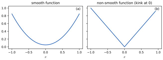
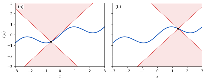
pp. 281–282 A function is Lipschitz with constant \(L\) if \(|f(x_1)-f(x_2)|\le L|x_1-x_2|\) (8.11): its graph stays outside a double cone of slope \(L\) placed at any of its points (Figure 8.8). For optimisation the relevant smoothness is that of the gradient: \(\cL\) is \(L\)-smooth if \(\|\nabla\cL(\bm x)-\nabla\cL(\bm y)\|\le L\|\bm x-\bm y\|\), which for twice differentiable \(\cL\) means \(-L\bm I\preceq\nabla^2\cL\preceq L\bm I\). A composite objective \(\cL=\cL_s+\cL_r\) (8.12) has a smooth part (the data loss) and a non-smooth part (a regulariser such as \(\|\bth\|_1\)).
Result 8.4 (the descent lemma)
If \(\cL\) is \(L\)-smooth then for all \(\bm x,\bm y\) \[ \cL(\bm y)\le\cL(\bm x)+\nabla\cL(\bm x)^\T(\bm y-\bm x)+\frac L2\|\bm y-\bm x\|^2. \] In particular a gradient step \(\bm y=\bm x-\eta\nabla\cL(\bm x)\) gives \(\cL(\bm y)\le\cL(\bm x)-\eta\big(1-\frac{L\eta}2\big)\|\nabla\cL(\bm x)\|^2\).
Proof
By the fundamental theorem of calculus along the segment, \[\cL(\bm y)-\cL(\bm x)-\nabla\cL(\bm x)^\T(\bm y-\bm x)=\int_0^1\big(\nabla\cL(\bm x+t(\bm y-\bm x))-\nabla\cL(\bm x)\big)^\T(\bm y-\bm x)\,dt. \] By Cauchy–Schwarz and the Lipschitz bound the integrand is at most \(Lt\|\bm y-\bm x\|^2\), and \(\int_0^1Lt\,dt=L/2\). Substituting \(\bm y-\bm x=-\eta\nabla\cL(\bm x)\) gives the second statement. \(\square\)
8.1.4.1 Subgradients
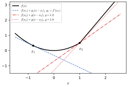
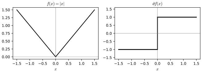
pp. 282–283 For convex \(f\), \(\bm g\) is a subgradient at \(\bm x\) if \[ f(\bm z)\ge f(\bm x)+\bm g^\T(\bm z-\bm x)\quad\text{for all }\bm z\in\dom f, \tag{8.13} \] and the set of subgradients is the subdifferential \(\partial f(\bm x)\). For the absolute value, \[ \partial|x|=\{-1\}\ (x<0),\qquad[-1,1]\ (x=0),\qquad\{+1\}\ (x>0). \tag{8.14} \]
Filling the gap 8.3: computing subdifferentials, and the optimality condition \(\bm 0\in\partial f(\bm x^*)\) pp. 277, 282
Derivation
(8.14). For \(x>0\) and \(0<\varepsilon<x\), (8.13) at \(z=x\pm\varepsilon\) gives \(x+\varepsilon\ge x+g\varepsilon\) and \(x-\varepsilon\ge x-g\varepsilon\), i.e. \(g\le1\) and \(g\ge1\); so \(\partial|x|=\{1\}\), and symmetrically \(\{-1\}\) for \(x<0\). At \(x=0\), (8.13) reads \(|z|\ge gz\) for all \(z\), which holds iff \(|g|\le1\).
Differentiable points. If \(f\) is convex and differentiable at \(\bm x\), then \(\partial f(\bm x)=\{\nabla f(\bm x)\}\): \(\nabla f(\bm x)\) is a subgradient by Result 8.2(a), and any subgradient \(\bm g\) satisfies \(f(\bm x+\varepsilon\bm d)-f(\bm x)\ge\varepsilon\bm g^\T\bm d\); dividing by \(\varepsilon\downarrow0\) gives \(\nabla f(\bm x)^\T\bm d\ge\bm g^\T\bm d\) for every \(\bm d\), and with \(\pm\bm d\) equality, so \(\bm g=\nabla f(\bm x)\).
Optimality. \(\bm 0\in\partial f(\bm x^*)\) means \(f(\bm z)\ge f(\bm x^*)\) for all \(\bm z\): it is exactly global minimality, with no smoothness needed. This is how the soft-thresholding operator of Section 8.6.2 and Exercise 8.1 are derived. \(\square\)
8.2 First-order methods
pp. 282–283 First-order methods use gradients only. From a start \(\bth_0\) they iterate \[ \bth_{t+1}=\bth_t+\eta_t\bm d_t \tag{8.15} \] with step size (learning rate) \(\eta_t\) and a descent direction \(\bm d_t\), such as \(-\bm g_t\).
See also (companion): Foundations of Deep Learning, 7.2 gradient descent, Bayesian and Probabilistic ML, 5.2.4.
8.2.1 Descent direction
p. 284 \(\bm d\) is a descent direction if \(\cL(\bth+\eta\bm d)<\cL(\bth)\) for all \(0<\eta<\eta_{\max}\) (8.16). With \(\bm g_t=\nabla\cL(\bth_t)\) (8.17), any \(\bm d\) with \[ \bm d^\T\bm g_t=\|\bm d\|\,\|\bm g_t\|\cos\vartheta<0 \tag{8.18} \] is a descent direction, where \(\vartheta\) is the angle between \(\bm d\) and \(\bm g_t\) (so \(\bm d\) is within \(90^\circ\) of \(-\bm g_t\)). Proof: \(\varphi(\eta)=\cL(\bth_t+\eta\bm d)\) has \(\varphi'(0)=\bm d^\T\bm g_t<0\), so by the definition of the derivative \(\varphi(\eta)<\varphi(0)\) for all small \(\eta>0\). Among unit vectors, \(-\bm g_t/\|\bm g_t\|\) minimises \(\bm d^\T\bm g_t\) (Cauchy–Schwarz): the steepest descent direction.
8.2.2 Step size (learning rate)
8.2.2.1 Constant step size
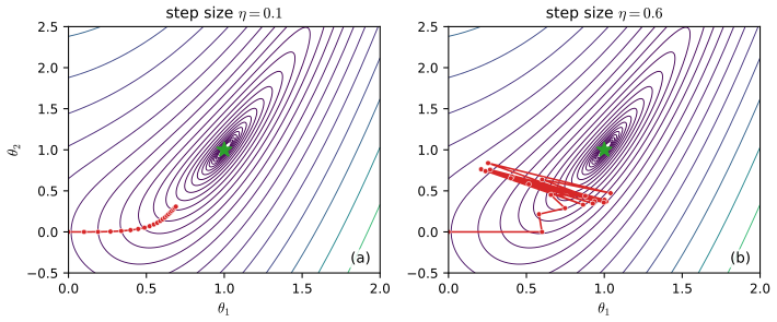
pp. 284–285 The book's example is \[ \cL(\bth)=0.5(\theta_1^2-\theta_2)^2+0.5(\theta_1-1)^2, \tag{8.19} \] minimised at \((1,1)\). Figure 8.11 runs 20 steps of \(\bth_{t+1}=\bth_t-\eta\bm g_t\) from \((0,0)\). The book calls (8.19) convex; it is not (see the notes on the book): at \((0,1)\) the Hessian is \(\diag(-1,1)\), and \(\cL(0,1)=1\) exceeds the average \(0.906\) of \(\cL(\pm0.5,1)\). Near the minimum it behaves like a quadratic with Hessian eigenvalues \(3\pm2\sqrt2\approx5.83,\ 0.17\), which explains the figure through (8.20): steps above \(2/5.83=0.34\) cannot settle at the minimum.
Result 8.5 (the step-size bound (8.20) and its general form) pp. 284–285
(a) For \(\cL(\bth)=\frac12\bth^\T\bm A\bth+\bm b^\T\bth+c\) with \(\bm A\succ0\), constant-step gradient descent converges to \(\bth^*=-\bm A^{-1}\bm b\) from every start iff \[ 0<\eta<\frac2{\lambda_{\max}(\bm A)}. \tag{8.20} \] The error contracts by \(\max_i|1-\eta\lambda_i|\) per step, minimised by \(\eta=2/(\lambda_{\min}+\lambda_{\max})\) at the rate \((\kappa-1)/(\kappa+1)\). (b) For any \(L\)-smooth \(\cL\) bounded below, \(0<\eta<2/L\) makes \(\cL(\bth_t)\) decrease at every step and \(\nabla\cL(\bth_t)\to\bm 0\).
Proof
(a) Since \(\bm g_t=\bm A(\bth_t-\bth^*)\), the error \(\bm e_t=\bth_t-\bth^*\) obeys \(\bm e_{t+1}=(\bm I-\eta\bm A)\bm e_t\). In the eigenbasis of \(\bm A\) the components evolve independently, \(e_{t+1,i}=(1-\eta\lambda_i)e_{t,i}\), so \(\bm e_t\to\bm 0\) for every \(\bm e_0\) iff \(|1-\eta\lambda_i|<1\), i.e. \(0<\eta\lambda_i<2\), for all \(i\); the binding case is \(\lambda_{\max}\). The contraction factor \(\max(|1-\eta\lambda_{\min}|,|1-\eta\lambda_{\max}|)\) is smallest when the two are equal, \(1-\eta\lambda_{\min}=\eta\lambda_{\max}-1\), giving \(\eta=2/(\lambda_{\min}+\lambda_{\max})\) and factor \((\lambda_{\max}-\lambda_{\min})/(\lambda_{\max}+\lambda_{\min})\). (If \(\bm A\) is only positive semidefinite, the components in its null space never move, and the iterates converge to a minimiser iff \(\bm b\) is in the range of \(\bm A\) and the same bound holds for the nonzero eigenvalues.)
(b) Result 8.4 gives \(\cL(\bth_{t+1})\le\cL(\bth_t)-c\|\bm g_t\|^2\) with \(c=\eta(1-L\eta/2)>0\). Summing from 0 to \(T-1\), \(c\sum_t\|\bm g_t\|^2\le\cL(\bth_0)-\inf\cL<\infty\), so \(\|\bm g_t\|\to0\) and \(\min_{t<T}\|\bm g_t\|^2\le(\cL(\bth_0)-\inf\cL)/(cT)\). This is "global convergence" to stationary points in the sense of Section 8.1.1; for the general \(L\)-smooth case, \(2/L\) is the analogue of \(2/\lambda_{\max}\). \(\square\)
See also (companion): the step-size demo of Foundations of Deep Learning, which plots the factors \(|1-\eta\lambda_i|\).
8.2.2.2 Line search
pp. 285–286 Exact line search picks \(\eta_t=\argmin_{\eta>0}\varphi_t(\eta)\), \(\varphi_t(\eta)=\cL(\bth_t+\eta\bm d_t)\) (8.21), a convex one-dimensional problem when \(\cL\) is convex. For the quadratic (8.22), \(\varphi'(\eta)=\bm d^\T(\bm A\bth+\bm b)+\eta\bm d^\T\bm A\bm d\) (8.23)–(8.25), so \[ \eta=-\frac{\bm d^\T(\bm A\bth+\bm b)}{\bm d^\T\bm A\bm d}. \tag{8.26} \] Inexact searches only ask for sufficient decrease, the Armijo condition \[ \cL(\bth_t+\eta\bm d_t)\le\cL(\bth_t)+c\,\eta\,\bm d_t^\T\nabla\cL(\bth_t),\qquad c\in(0,1),\ \text{typically }10^{-4}, \tag{8.27} \] enforced by backtracking: start at \(\eta_0\) and multiply by \(\rho\in(0,1)\) until (8.27) holds.
Filling the gap 8.4: backtracking stops, and the accepted step is not too small p. 286
Derivation
Take \(\bm d=-\bm g\) and an \(L\)-smooth \(\cL\). By Result 8.4, \(\cL(\bth-\eta\bm g)\le\cL(\bth)-\eta(1-L\eta/2)\|\bm g\|^2\), and the right side is at most \(\cL(\bth)-c\eta\|\bm g\|^2\), which is (8.27), as soon as \(1-L\eta/2\ge c\), i.e. \(\eta\le2(1-c)/L\). Backtracking from \(\eta_0\) therefore stops after at most \(1+\lceil\log(\eta_0L/(2(1-c)))/\log(1/\rho)\rceil\) trials, with an accepted step \(\eta\ge\min\{\eta_0,\,2\rho(1-c)/L\}\) (it stops at the first trial value below the threshold, or earlier). The decrease per step is then at least \(c\min\{\eta_0,2\rho(1-c)/L\}\|\bm g\|^2\), so the conclusions of Result 8.5(b) hold without knowing \(L\). For a general descent direction the same argument works with \(\bm d^\T\bm g<0\) in place of \(-\|\bm g\|^2\). \(\square\)
8.2.3 Convergence rates
pp. 286–287 A method converges linearly with rate \(\mu\in(0,1)\) if \(|\cL(\bth_{t+1})-\cL(\bth^*)|\le\mu|\cL(\bth_t)-\cL(\bth^*)|\) (8.28). For steepest descent with exact line search on a quadratic with \(\bm A\succ0\), \[ \mu=\Big(\frac{\lambda_{\max}-\lambda_{\min}}{\lambda_{\max}+\lambda_{\min}}\Big)^2=\Big(\frac{\kappa-1}{\kappa+1}\Big)^2,\qquad\kappa=\frac{\lambda_{\max}}{\lambda_{\min}}. \tag{8.29} \]
Result 8.6 (the rate (8.29) of exact line search, via the Kantorovich inequality) p. 286
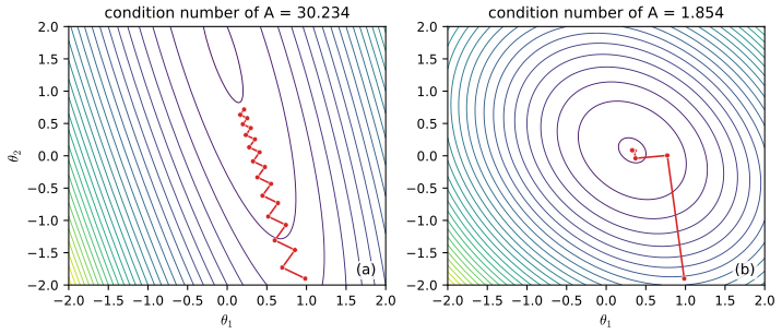
For \(\cL=\frac12\bth^\T\bm A\bth+\bm b^\T\bth+c\), \(\bm A\succ0\), steepest descent with the exact step (8.26) satisfies \(\cL(\bth_{t+1})-\cL^*\le\mu\,(\cL(\bth_t)-\cL^*)\) with \(\mu\) as in (8.29), and the bound is attained at every step when the gradient has equal weight on the eigenvectors of \(\lambda_{\min}\) and \(\lambda_{\max}\). Consecutive gradients are orthogonal, \(\bm g_{t+1}^\T\bm g_t=0\), which produces the zig-zag.
Proof
Write \(\bm e=\bth_t-\bth^*\) and \(\bm g=\bm A\bm e\). Then \(\cL(\bth_t)-\cL^*=\frac12\bm e^\T\bm A\bm e=\frac12\bm g^\T\bm A^{-1}\bm g\). With \(\bm d=-\bm g\), (8.26) gives \(\eta=\bm g^\T\bm g/\bm g^\T\bm A\bm g\) and \[ \cL(\bth_t-\eta\bm g)=\cL(\bth_t)-\eta\,\bm g^\T\bm g+\tfrac12\eta^2\bm g^\T\bm A\bm g=\cL(\bth_t)-\frac{(\bm g^\T\bm g)^2}{2\,\bm g^\T\bm A\bm g}, \] so \[ \frac{\cL(\bth_{t+1})-\cL^*}{\cL(\bth_t)-\cL^*}=1-\frac{(\bm g^\T\bm g)^2}{(\bm g^\T\bm A\bm g)(\bm g^\T\bm A^{-1}\bm g)}. \] Kantorovich inequality: for \(\bm A\succ0\) with extreme eigenvalues \(m\le M\), \((\bm g^\T\bm A\bm g)(\bm g^\T\bm A^{-1}\bm g)\le\frac{(M+m)^2}{4Mm}(\bm g^\T\bm g)^2\). To prove it, normalise \(\|\bm g\|=1\) and let \(p_i\ge0\), \(\sum p_i=1\), be the squared coordinates of \(\bm g\) in the eigenbasis, so the two factors are \(\bar\lambda=\sum p_i\lambda_i\) and \(\sum p_i/\lambda_i\). For \(\lambda\in[m,M]\), \((\lambda-m)(\lambda-M)\le0\), which after dividing by \(\lambda Mm\) reads \(1/\lambda\le(M+m-\lambda)/(Mm)\). Averaging, \(\sum p_i/\lambda_i\le(M+m-\bar\lambda)/(Mm)\), and \(\bar\lambda(M+m-\bar\lambda)\le(M+m)^2/4\) (a parabola in \(\bar\lambda\) with maximum at \((M+m)/2\)). Hence the ratio is at most \(1-\frac{4Mm}{(M+m)^2}=\big(\frac{M-m}{M+m}\big)^2\). Equality needs \(p\) concentrated on \(m\) and \(M\) with \(\bar\lambda=(M+m)/2\), i.e. weights \(\frac12,\frac12\).
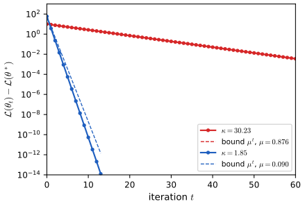
Orthogonality. \(\bm g_{t+1}=\bm A(\bth_t-\eta\bm g)+\bm b=\bm g-\eta\bm A\bm g\), so \(\bm g^\T\bm g_{t+1}=\bm g^\T\bm g-\eta\bm g^\T\bm A\bm g=0\) by the choice of \(\eta\). In two dimensions this forces the gradients to alternate between two fixed directions; if the first gradient has equal weights, so do all later ones, and the bound is attained at every step: Figures 8.12a and 8.S1 show the measured ratio \(0.876033=\mu\) for \(\kappa=30.234\). \(\square\)
Result 8.7 (rates of gradient descent) p. 286
Let \(\cL\) be convex and \(L\)-smooth with a minimiser \(\bth^*\), and run \(\bth_{t+1}=\bth_t-\frac1L\nabla\cL(\bth_t)\). (a) \(\cL(\bth_t)-\cL^*\le\dfrac{L\|\bth_0-\bth^*\|^2}{2t}\) (sublinear). (b) If \(\cL\) is also \(m\)-strongly convex, \(\cL(\bth_{t+1})-\cL^*\le(1-\tfrac1\kappa)(\cL(\bth_t)-\cL^*)\) with \(\kappa=L/m\): the linear rate (8.28) with \(\mu=1-1/\kappa\). Strong convexity (or the Polyak–Łojasiewicz inequality of Result 8.3) is what makes the rate linear: on \(\cL=\theta^4\), convex and smooth near the optimum, gradient descent is only sublinear.
Proof
Write \(\bm g=\nabla\cL(\bth)\) and \(\bth^+=\bth-\bm g/L\). Result 8.4 gives \(\cL(\bth^+)\le\cL(\bth)-\frac1{2L}\|\bm g\|^2\) (monotone decrease).
(a) Convexity gives \(\cL(\bth)\le\cL^*+\bm g^\T(\bth-\bth^*)\). Combining, \[ \cL(\bth^+)-\cL^*\le\bm g^\T(\bth-\bth^*)-\frac1{2L}\|\bm g\|^2=\frac L2\Big(\|\bth-\bth^*\|^2-\big\|\bth-\bth^*-\tfrac1L\bm g\big\|^2\Big)=\frac L2\big(\|\bth-\bth^*\|^2-\|\bth^+-\bth^*\|^2\big). \] Summing over the first \(t\) steps the right side telescopes: \(\sum_{s=1}^t(\cL(\bth_s)-\cL^*)\le\frac L2\|\bth_0-\bth^*\|^2\). The terms decrease, so the last is at most the average: \(t(\cL(\bth_t)-\cL^*)\le\frac L2\|\bth_0-\bth^*\|^2\).
(b) By Result 8.3, \(\|\bm g\|^2\ge2m(\cL(\bth)-\cL^*)\). Then \(\cL(\bth^+)-\cL^*\le\cL(\bth)-\cL^*-\frac mL(\cL(\bth)-\cL^*)\).
The counterexample. For \(\cL=\theta^4\) and step \(\eta\), \(\theta_{t+1}=\theta_t(1-4\eta\theta_t^2)\): the contraction factor tends to 1 as \(\theta_t\to0\), and \(\theta_t\sim(8\eta t)^{-1/2}\), not geometric. Both rates were confirmed numerically on the logistic loss used in Figure 8.S3 (\(m=0.01\)). \(\square\)
p. 286 Near a local optimum a smooth objective is close to its quadratic model, so \(\kappa(\bm H)\) at the optimum governs the local rate; second-order methods (Section 8.3) remove the dependence on \(\kappa\), and conjugate gradients remove the zig-zag for quadratics (Shewchuk, 1994).
8.2.4 Momentum methods
8.2.4.1 Momentum
pp. 287–288 The heavy-ball method (Polyak, 1964) is \[ \bm m_t=\beta\bm m_{t-1}+\bm g_{t-1},\qquad\bth_t=\bth_{t-1}-\eta_t\bm m_t, \tag{8.30, 8.31} \] with \(0<\beta<1\), typically 0.9. Unrolling, \(\bm m_t=\sum_{\tau=0}^{t-1}\beta^\tau\bm g_{t-\tau-1}\) (8.32), a discounted sum of past gradients; for a constant gradient \(\bm m_t=\bm g\sum_{\tau=0}^{t-1}\beta^\tau\to\bm g/(1-\beta)\) (8.33)–(8.34), a tenfold step for \(\beta=0.9\).
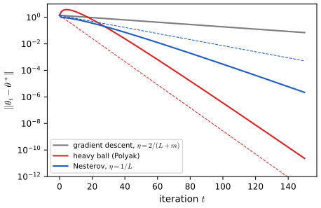
Filling the gap 8.5: why momentum helps on ill-conditioned problems, with Polyak's parameters
Derivation
On \(\cL=\frac12\bth^\T\bm A\bth\) with eigenvalues in \([m,L]\), eliminating \(\bm m\) from (8.30)–(8.31) gives the two-step recursion \(\bth_{t+1}=\bth_t-\eta\bm A\bth_t+\beta(\bth_t-\bth_{t-1})\). Along an eigenvector with eigenvalue \(\lambda\) the coordinate obeys \(e_{t+1}=(1+\beta-\eta\lambda)e_t-\beta e_{t-1}\), whose characteristic polynomial is \(z^2-(1+\beta-\eta\lambda)z+\beta\). If its discriminant is non-positive, \(|1+\beta-\eta\lambda|\le2\sqrt\beta\), the two roots are complex conjugates (or a double root) with product \(\beta\), hence modulus \(\sqrt\beta\), and the coordinate decays like \(\sqrt\beta^{\,t}\) (times \(t\) for a double root). The condition is equivalent to \((1-\sqrt\beta)^2\le\eta\lambda\le(1+\sqrt\beta)^2\). Choose \[ \eta=\frac4{(\sqrt L+\sqrt m)^2},\qquad\beta=\Big(\frac{\sqrt\kappa-1}{\sqrt\kappa+1}\Big)^2: \] then \((1-\sqrt\beta)^2=\frac4{(\sqrt\kappa+1)^2}=\eta m\) and \((1+\sqrt\beta)^2=\frac{4\kappa}{(\sqrt\kappa+1)^2}=\eta L\), so every \(\lambda\in[m,L]\) satisfies the condition and every mode contracts at rate \(\sqrt\beta=\frac{\sqrt\kappa-1}{\sqrt\kappa+1}\). Plain gradient descent achieves at best \(\frac{\kappa-1}{\kappa+1}\) (Result 8.5). For \(\kappa=100\) the factors are \(0.818\) and \(0.980\): about 10 times fewer iterations for the same accuracy (Figure 8.S2; the measured rate was 0.8205). For non-quadratic functions the heavy ball has no such global guarantee, which is one motivation for Nesterov's method. \(\square\)
See also (companion): Foundations of Deep Learning, 7.3.1 momentum and the optimiser paths demo.
8.2.4.2 Nesterov momentum
pp. 288–289 Nesterov's accelerated gradient evaluates the gradient after an extrapolation: \[ \tilde\bth_{t+1}=\bth_t+\beta(\bth_t-\bth_{t-1}),\qquad\bth_{t+1}=\tilde\bth_{t+1}-\eta_t\nabla\cL(\tilde\bth_{t+1}), \tag{8.35, 8.36} \] equivalently \[ \bm m_{t+1}=\beta\bm m_t-\eta_t\nabla\cL(\bth_t+\beta\bm m_t),\qquad\bth_{t+1}=\bth_t+\bm m_{t+1}. \tag{8.37, 8.38} \] (The book's Figure 8.13, a vector sketch of the look-ahead, is not reproduced; Figure 8.S2 shows the method at work.)
Filling the gap 8.6: the two forms are the same method, and what "accelerated" means pp. 288–289
Derivation
Equivalence. Define \(\bm m_t=\bth_t-\bth_{t-1}\) (with \(\bth_{-1}=\bth_0\), so \(\bm m_0=\bm 0\)). Then (8.35)–(8.36) say \(\bth_{t+1}=\bth_t+\beta\bm m_t-\eta_t\nabla\cL(\bth_t+\beta\bm m_t)\); subtracting \(\bth_t\), \(\bm m_{t+1}=\beta\bm m_t-\eta_t\nabla\cL(\bth_t+\beta\bm m_t)\), which is (8.37), and \(\bth_{t+1}=\bth_t+\bm m_{t+1}\) is (8.38). Both forms produce identical iterates (confirmed numerically to rounding error). Compared with (8.30)–(8.31), the only change is where the gradient is evaluated.
Rates. For convex \(L\)-smooth \(\cL\), with \(\eta=1/L\) and the schedule \(\beta_t=(s_t-1)/s_{t+1}\), \(s_1=1\), \(s_{t+1}=\frac12(1+\sqrt{1+4s_t^2})\), the method satisfies \(\cL(\bth_t)-\cL^*\le\frac{2L\|\bth_0-\bth^*\|^2}{(t+1)^2}\). This is the special case \(\cL_r=0\) of Result 8.15 below (FISTA), where the proof is given in full. The \(O(1/t^2)\) rate cannot be improved by any method that only combines gradients (Nesterov, 2004), against \(O(1/t)\) for gradient descent (Result 8.7): that is the sense of "accelerated". For \(m\)-strongly convex functions a constant \(\beta=\frac{\sqrt\kappa-1}{\sqrt\kappa+1}\) gives the linear rate \(1-1/\sqrt\kappa\) in function value, against \(1-1/\kappa\). \(\square\)
8.3 Second-order methods
p. 289 Second-order methods use curvature (the Hessian or an approximation of it) to rescale the gradient, which removes the dependence on the condition number seen in Figure 8.12.
See also (companion): Bayesian and Probabilistic ML, 5.2.2 local quadratic approximation, 5.4 the Hessian matrix.
8.3.1 Newton's method
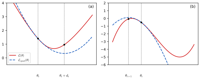
pp. 289–290 Newton's method takes \[ \bth_{t+1}=\bth_t-\eta_t\bm H_t^{-1}\bm g_t,\qquad\bm H_t=\nabla^2\cL(\bth_t), \tag{8.39, 8.40} \] the minimiser of the second-order Taylor model \[ \cL_{\rm quad}(\bth)=\cL(\bth_t)+\bm g_t^\T(\bth-\bth_t)+\tfrac12(\bth-\bth_t)^\T\bm H_t(\bth-\bth_t), \tag{8.41} \] which is \(\bth=\bth_t-\bm H_t^{-1}\bm g_t\) (8.42).
Algorithm 8.1: Newton's method for minimising a function p. 289
- Initialise \(\bth_0\).
- For \(t=0,1,2,\dots\) until convergence: evaluate \(\bm g_t=\nabla\cL(\bth_t)\) and \(\bm H_t=\nabla^2\cL(\bth_t)\); solve \(\bm H_t\bm d_t=-\bm g_t\); choose \(\eta_t\) by line search along \(\bm d_t\) (pure Newton: \(\eta_t=1\)); set \(\bth_{t+1}=\bth_t+\eta_t\bm d_t\).
Filling the gap 8.7: when the Newton step descends, and the one-step solution of least squares pp. 289–290, (8.42)–(8.43)
Derivation
(8.42). \(\nabla\cL_{\rm quad}(\bth)=\bm g_t+\bm H_t(\bth-\bth_t)\) vanishes at \(\bth_t-\bm H_t^{-1}\bm g_t\). This is the minimiser of the model iff \(\bm H_t\succeq0\) (unique iff \(\bm H_t\succ0\)); if \(\bm H_t\) has a negative eigenvalue the stationary point is a saddle or maximum of the model, the situation of Figure 8.14b. The Newton direction \(\bm d=-\bm H_t^{-1}\bm g_t\) has \(\bm d^\T\bm g_t=-\bm g_t^\T\bm H_t^{-1}\bm g_t\), negative when \(\bm H_t\succ0\), so then it is a descent direction (8.18), and a line search makes every iteration decrease \(\cL\).
(8.43). For least squares \(\cL(\bm w)=\frac12\|\bm X\bm w-\bm y\|^2\), \(\bm g=\bm X^\T\bm X\bm w-\bm X^\T\bm y\) and \(\bm H=\bm X^\T\bm X\) does not depend on \(\bm w\): the quadratic model is the function itself, so one pure Newton step from any \(\bm w_0\) lands on \((\bm X^\T\bm X)^{-1}\bm X^\T\bm y\) (confirmed numerically to \(10^{-10}\)). Newton's method is also invariant to affine reparametrisations \(\bth=\bm B\bm\phi\): the iterates in \(\bm\phi\) map exactly to those in \(\bth\), which is why the condition number does not matter. \(\square\)
Result 8.8 (local quadratic convergence of Newton's method)
Suppose \(\nabla^2\cL\) is Lipschitz with constant \(M\) near a minimiser \(\bth^*\) with \(\nabla^2\cL(\bth^*)\succeq\mu\bm I\), \(\mu>0\). If \(\|\bth_0-\bth^*\|\le\mu/(2M)\), pure Newton steps satisfy \[ \|\bth_{t+1}-\bth^*\|\le\frac M\mu\,\|\bth_t-\bth^*\|^2 , \] so the number of correct digits roughly doubles at every step.
Proof
Let \(\bm e=\bth_t-\bth^*\). Since \(\bm g^*=\bm 0\), \(\bm g_t=\int_0^1\nabla^2\cL(\bth^*+s\bm e)\bm e\,ds\), so \[ \bth_{t+1}-\bth^*=\bm e-\bm H_t^{-1}\bm g_t=\bm H_t^{-1}\int_0^1\big(\bm H_t-\nabla^2\cL(\bth^*+s\bm e)\big)\bm e\,ds. \] The Lipschitz bound gives \(\|\bm H_t-\nabla^2\cL(\bth^*+s\bm e)\|\le M(1-s)\|\bm e\|\), and \(\int_0^1(1-s)ds=\frac12\). Also \(\|\bm H_t-\nabla^2\cL(\bth^*)\|\le M\|\bm e\|\le\mu/2\), so the smallest eigenvalue of \(\bm H_t\) is at least \(\mu/2\) and \(\|\bm H_t^{-1}\|\le2/\mu\). Together, \(\|\bth_{t+1}-\bth^*\|\le\frac2\mu\cdot\frac M2\|\bm e\|^2\). Because \(\frac M\mu\|\bm e\|\le\frac12\), the next error is at most half the current one, the iterates stay in the ball, and the argument repeats. On the Rosenbrock function the ratios \(e_{t+1}/e_t^2\) stayed between 1 and 2.4 until machine precision. \(\square\)
p. 290 Far from the optimum the pure step can overshoot or go uphill; a line search (Algorithm 8.1) or a trust region (Section 8.3.3) is needed. For logistic regression Newton's method takes several iterations (Section 10.2.6 of the book).
8.3.2 BFGS and other quasi-Newton methods
pp. 290–291 BFGS keeps an approximation \(\bm B_t\approx\bm H_t\) updated by a rank-two correction, \[ \bm B_{t+1}=\bm B_t+\frac{\bm y_t\bm y_t^\T}{\bm y_t^\T\bm s_t}-\frac{(\bm B_t\bm s_t)(\bm B_t\bm s_t)^\T}{\bm s_t^\T\bm B_t\bm s_t},\qquad\bm s_t=\bth_t-\bth_{t-1},\quad\bm y_t=\bm g_t-\bm g_{t-1}, \tag{8.44–8.46} \] or, equivalently, an approximation \(\bm C_t\approx\bm H_t^{-1}\) of the inverse, \[ \bm C_{t+1}=\Big(\bm I-\frac{\bm s_t\bm y_t^\T}{\bm y_t^\T\bm s_t}\Big)\bm C_t\Big(\bm I-\frac{\bm y_t\bm s_t^\T}{\bm y_t^\T\bm s_t}\Big)+\frac{\bm s_t\bm s_t^\T}{\bm y_t^\T\bm s_t}. \tag{8.48} \] The step size should satisfy the Wolfe conditions: the Armijo condition (8.27) and the curvature condition, which in its standard form reads \[ \bm d_t^\T\nabla\cL(\bth_t+\eta\bm d_t)\ge c_2\,\bm d_t^\T\nabla\cL(\bth_t),\qquad c_2\in(c,1) \tag{8.47} \] (the book's display drops the inner product with \(\bm d_t\) on the left and has a stray \(\eta\) on the right). L-BFGS stores only the last \(M\) pairs \((\bm s,\bm y)\), \(M\) between 5 and 20, and applies \(\bm C_t\) to a vector in \(O(MD)\) operations by unrolling (8.48) in two loops; scikit-learn's logistic regression uses it by default.
Result 8.9 (the BFGS update: secant equation, positive definiteness, and the inverse form) pp. 290–291
Let \(\bm B_t\succ0\), \(\bm C_t=\bm B_t^{-1}\) and \(\rho=1/(\bm y^\T\bm s)\). (a) \(\bm B_{t+1}\bm s=\bm y\) and \(\bm C_{t+1}\bm y=\bm s\) (the secant equations: the new model reproduces the observed change in gradient). (b) \(\bm B_{t+1}\succ0\) iff \(\bm y^\T\bm s>0\). (c) If \(\bm d_t^\T\bm g_t<0\) and the step satisfies the curvature condition (8.47) with \(c_2<1\), then \(\bm y^\T\bm s>0\). (d) (8.48) is the inverse of (8.44): \(\bm C_{t+1}=\bm B_{t+1}^{-1}\).
Proof
(a) \(\bm B_{t+1}\bm s=\bm B\bm s+\bm y\frac{\bm y^\T\bm s}{\bm y^\T\bm s}-\bm B\bm s\frac{\bm s^\T\bm B\bm s}{\bm s^\T\bm B\bm s}=\bm y\). With \(\bm V=\bm I-\rho\bm s\bm y^\T\), \(\bm V^\T\bm y=\bm y-\rho\bm y(\bm s^\T\bm y)=\bm 0\), so \(\bm C_{t+1}\bm y=\bm V\bm C\bm V^\T\bm y+\rho\bm s(\bm s^\T\bm y)=\bm s\).
(b) For \(\bm v\ne\bm 0\), \[ \bm v^\T\bm B_{t+1}\bm v=\Big(\bm v^\T\bm B\bm v-\frac{(\bm v^\T\bm B\bm s)^2}{\bm s^\T\bm B\bm s}\Big)+\frac{(\bm y^\T\bm v)^2}{\bm y^\T\bm s}. \] The bracket is non-negative by the Cauchy–Schwarz inequality for the inner product \(\langle\bm u,\bm w\rangle=\bm u^\T\bm B\bm w\), and zero only if \(\bm v=\alpha\bm s\). If \(\bm y^\T\bm s>0\) the last term is non-negative, and for \(\bm v=\alpha\bm s\) it equals \(\alpha^2\bm y^\T\bm s>0\); so the sum is positive for every \(\bm v\ne\bm 0\). Conversely, if \(\bm B_{t+1}\succ0\) then by (a) \(\bm y^\T\bm s=\bm s^\T\bm B_{t+1}\bm s>0\).
(c) \(\bm s=\eta\bm d_t\), so \[\bm y^\T\bm s=\eta\big(\bm d_t^\T\nabla\cL(\bth_{t+1})-\bm d_t^\T\bm g_t\big)\ge\eta(c_2-1)\bm d_t^\T\bm g_t>0. \]
(d) The vectors \(\bm y\) and \(\bm s^\perp=\{\bm w:\bm s^\T\bm w=0\}\) span \(\R^D\) because \(\bm s^\T\bm y\ne0\); it suffices to check \(\bm B_{t+1}\bm C_{t+1}\bm v=\bm v\) on them. For \(\bm y\): \(\bm B_{t+1}\bm C_{t+1}\bm y=\bm B_{t+1}\bm s=\bm y\) by (a). For \(\bm w\in\bm s^\perp\): \(\bm V^\T\bm w=\bm w\), so \(\bm C_{t+1}\bm w=\bm V\bm C\bm w=\bm C\bm w-\rho\bm s(\bm y^\T\bm C\bm w)\), and \[ \bm B_{t+1}\bm C\bm w=\bm w+\rho\bm y(\bm y^\T\bm C\bm w)-\frac{\bm B\bm s\,(\bm s^\T\bm w)}{\bm s^\T\bm B\bm s}=\bm w+\rho\bm y(\bm y^\T\bm C\bm w), \] while \(\bm B_{t+1}\bm s=\bm y\); hence \[\bm B_{t+1}\bm C_{t+1}\bm w=\bm w+\rho\bm y(\bm y^\T\bm C\bm w)-\rho(\bm y^\T\bm C\bm w)\bm y=\bm w. \] \(\square\)
All four statements were confirmed numerically on random pairs; in the run of the demonstration on the Rosenbrock function every \(\bm C_t\) stayed positive definite.
8.3.3 Trust region methods
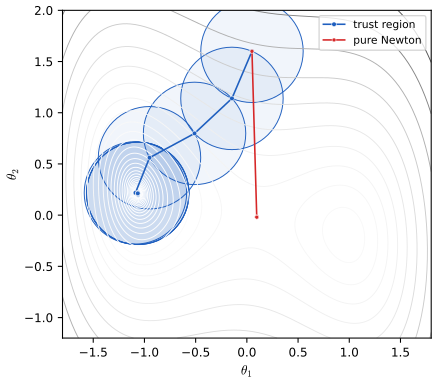
pp. 291–292 When \(\bm H_t\) is not positive definite the Newton direction may point uphill. A trust-region method minimises the quadratic model \(M_t(\bm\delta)=\cL(\bth_t)+\bm g_t^\T\bm\delta+\frac12\bm\delta^\T\bm H_t\bm\delta\) (8.50) only over a region \(R_t\) where it is trusted, usually a ball \(\|\bm\delta\|\le r\) (8.49): it picks the distance first and then the best direction, the reverse of line search. With a multiplier \(\lambda\ge0\) for the ball, the solution has the form \[ \bm\delta=-(\bm H+\lambda\bm I)^{-1}\bm g, \tag{8.52} \] Tikhonov damping; \(\lambda\to0\) recovers Newton, large \(\lambda\) a short gradient step. The book's (8.51) adds \(\lambda\|\bm\delta\|^2\) to the model, which gives \(\bm H+2\lambda\bm I\) in (8.52); with the penalty \(\frac\lambda2\|\bm\delta\|^2\) the formula is as stated (a change of the constant only).
Result 8.10 (characterisation of the trust-region step; Moré and Sorensen, 1983) p. 292
\(\bm\delta^*\) minimises \(m(\bm\delta)=\bm g^\T\bm\delta+\frac12\bm\delta^\T\bm H\bm\delta\) over \(\|\bm\delta\|\le r\) (for any symmetric \(\bm H\)) iff \(\|\bm\delta^*\|\le r\) and there is \(\lambda\ge0\) with \[ (\bm H+\lambda\bm I)\bm\delta^*=-\bm g,\qquad\bm H+\lambda\bm I\succeq0,\qquad\lambda\,(r-\|\bm\delta^*\|)=0. \] So \(\lambda\ge\max(0,-\lambda_{\min}(\bm H))\): the damping lifts every negative eigenvalue of \(\bm H\) to a non-negative one. In the eigenbasis of \(\bm H\), \(\|\bm\delta(\lambda)\|^2=\sum_i\tilde g_i^2/(\lambda_i+\lambda)^2\) is decreasing in \(\lambda\), so \(\lambda\) is found by a one-dimensional search, which is how the code and the demonstration solve the subproblem exactly.
Proof of sufficiency
Expanding both sides and using \(\bm g=-(\bm H+\lambda\bm I)\bm\delta^*\), one checks the identity, valid for every \(\bm\delta\), \[ m(\bm\delta)=m(\bm\delta^*)+\tfrac12(\bm\delta-\bm\delta^*)^\T(\bm H+\lambda\bm I)(\bm\delta-\bm\delta^*)+\tfrac\lambda2\big(\|\bm\delta^*\|^2-\|\bm\delta\|^2\big). \] The middle term is non-negative because \(\bm H+\lambda\bm I\succeq0\). The last is non-negative for \(\|\bm\delta\|\le r\): either \(\lambda=0\), or \(\|\bm\delta^*\|=r\ge\|\bm\delta\|\). Hence \(m(\bm\delta)\ge m(\bm\delta^*)\) on the ball. Necessity is Theorem 4.1 of Nocedal and Wright (2006). The exact solver in the code was checked against a brute-force search of the disc for 20 random indefinite problems. \(\square\)
p. 291 A trust-region method compares the actual decrease \(\cL(\bth_t)-\cL(\bth_t+\bm\delta)\) with the predicted one \(M_t(\bm0)-M_t(\bm\delta)\): if the ratio is small the radius shrinks (and the step may be rejected); if it is close to 1 and the step reached the boundary, the radius grows.
8.4 Stochastic gradient descent
p. 292 In stochastic optimisation \(\cL(\bth)=\E_{q(\bm z)}[\cL(\bth,\bm z)]\) (8.53) and each step uses an unbiased estimate of the gradient, \[ \bth_{t+1}=\bth_t-\eta_t\nabla_{\bth}\cL(\bth_t,\bm z_t)=\bth_t-\eta_t\bm g_t,\qquad\bm z_t\sim q. \tag{8.54} \]
See also (companion): Foundations of Deep Learning, 7.2.3 SGD and 7.2.4 minibatches.
8.4.1 Application to finite sum problems
p. 293 Empirical risk minimisation is a finite sum, \(\cL(\bth)=\frac1N\sum_{n=1}^N\cL_n(\bth)\) (8.55), with gradient (8.56) costing \(N\) evaluations. A minibatch \(\mathcal B_t\) of size \(B\ll N\) gives \(\bm g_t\approx\frac1{|\mathcal B_t|}\sum_{n\in\mathcal B_t}\nabla\cL_n(\bth_t)\) (8.57). Per unit of computation SGD often wins early on, when the parameters are poor and an exact gradient is wasted effort.
Filling the gap 8.8: the minibatch gradient is unbiased, and its variance p. 293, (8.57)
Derivation
Fix \(\bth\), write \(\bm a_n=\nabla\cL_n(\bth)\), \(\bar{\bm a}=\frac1N\sum_n\bm a_n=\nabla\cL(\bth)\), and work with one coordinate \(a_n\) (the argument is coordinatewise), \(\sigma^2=\frac1N\sum_n(a_n-\bar a)^2\). Let \(Z_n=1\) if \(n\) is in the batch.
Without replacement (a uniformly random subset of size \(B\)): \(\E Z_n=B/N\), so \(\E\big[\frac1B\sum_nZ_na_n\big]=\bar a\): unbiased. For the variance, since \(\sum_nZ_n=B\) is fixed we may replace \(a_n\) by \(a_n-\bar a\) (which sum to zero). With \(\var Z_n=\frac BN(1-\frac BN)\) and, for \(n\ne n'\), \(\cov(Z_n,Z_{n'})=\frac{B(B-1)}{N(N-1)}-\frac{B^2}{N^2}=-\frac{B(N-B)}{N^2(N-1)}\), and using \(\sum_{n\ne n'}(a_n-\bar a)(a_{n'}-\bar a)=-\sum_n(a_n-\bar a)^2\), \[ \var\Big(\sum_nZ_na_n\Big)=N\sigma^2\Big[\frac{B(N-B)}{N^2}+\frac{B(N-B)}{N^2(N-1)}\Big]=\sigma^2\frac{B(N-B)}{N-1}, \] so the minibatch mean has variance \(\frac{\sigma^2}B\cdot\frac{N-B}{N-1}\). With replacement (independent uniform indices, as in the demonstration) the variance is \(\sigma^2/B\). Both vanish only if all \(\nabla\cL_n(\bth)\) coincide; at the optimum \(\bar a=0\) but \(\sigma^2>0\) in general, which is why constant-step SGD does not converge (Section 8.4.3). Checked by enumerating all subsets for \(N=7\). \(\square\)
8.4.2 Example: SGD for fitting linear regression
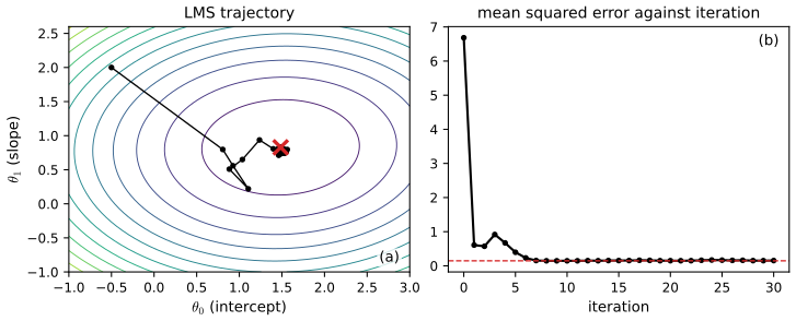
pp. 293–294 For \(\cL(\bth)=\frac1{2N}\|\bm X\bth-\bm y\|^2\) (8.58), with gradient (8.59), SGD with \(B=1\) is the least mean squares (LMS) or Widrow–Hoff rule \[ \bth_{t+1}=\bth_t-\eta_t(\bth_t^\T\bm x_n-y_n)\bm x_n. \tag{8.60} \]
See also (companion): the LMS demo of Foundations of Deep Learning.
8.4.3 Choosing the step size (learning rate)
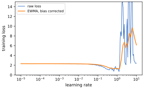
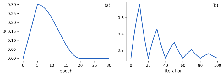
pp. 294–296 Too small a learning rate underfits, too large is unstable (Figure 8.17). The "learning-rate range test" trains briefly while increasing \(\eta\) and picks a value somewhat below the one with the lowest loss. Common schedules are \[ \eta_t=\eta_i\ \text{for}\ t_i\le t\le t_{i+1},\qquad\eta_t=\eta_0e^{-\lambda t},\qquad\eta_t=\eta_0(\beta t+1)^{-\alpha}, \tag{8.62–8.64} \] piecewise constant (step decay, or reduce-on-plateau when the milestones are adaptive), exponential (usually too fast) and polynomial (\(\alpha=0.5,\beta=1\) is the square-root schedule \(\eta_0/\sqrt{t+1}\)). Warm-up followed by a cosine decay, and cyclical schedules (with warm restarts and snapshot ensembles) are common in deep learning (Figure 8.19). Line searches can be used with SGD when the gradient noise vanishes at the optimum, as for models that interpolate the data.
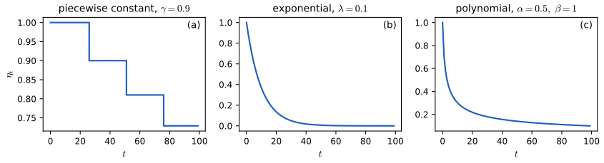
p. 295 The book states the Robbins–Monro conditions as \(\eta_t\to0\) and \(\sum_t\eta_t^2/\sum_t\eta_t\to0\) (8.61). The classical conditions of Robbins and Monro (1951) are \[ \sum_{t=1}^\infty\eta_t=\infty,\qquad\sum_{t=1}^\infty\eta_t^2<\infty: \] enough total movement to reach the optimum, and noise whose accumulated variance stays finite. Result 8.11 shows where each version comes from. Note that the recommended square-root schedule violates \(\sum\eta_t^2<\infty\) (\(\sum1/t\) diverges) but satisfies the ratio form, since \(\sum_{t\le T}\eta_t^2/\sum_{t\le T}\eta_t\approx\log T/(2\sqrt T)\to0\).
Result 8.11 (convergence of SGD and the two forms of the Robbins–Monro conditions) pp. 293, 295
Assume \(\E[\bm g_t\given\bth_t]=\nabla\cL(\bth_t)\) and \(\E\|\bm g_t\|^2\le G^2\), and let \(R=\|\bth_0-\bth^*\|\).
(a) If \(\cL\) is convex, the weighted average \(\bar\bth_T=\sum_{t<T}\eta_t\bth_t/\sum_{t<T}\eta_t\) satisfies \[ \E\,\cL(\bar\bth_T)-\cL^*\le\frac{R^2+G^2\sum_{t<T}\eta_t^2}{2\sum_{t<T}\eta_t}, \] which tends to 0 whenever \(\sum\eta_t=\infty\) and \(\sum_{t<T}\eta_t^2/\sum_{t<T}\eta_t\to0\) (the book's (8.61)). With \(\eta_t=\eta_0/\sqrt{t+1}\) the bound is \(O(\log T/\sqrt T)\).
(b) If \(\cL\) is \(m\)-strongly convex, \(a_t=\E\|\bth_t-\bth^*\|^2\) tends to 0 whenever \(\sum\eta_t=\infty\) and \(\sum\eta_t^2<\infty\) (the classical conditions), e.g. \(\eta_t=\eta_0/t\).
Proof
Expanding the update, \[\|\bth_{t+1}-\bth^*\|^2=\|\bth_t-\bth^*\|^2-2\eta_t\bm g_t^\T(\bth_t-\bth^*)+\eta_t^2\|\bm g_t\|^2. \] Conditioning on \(\bth_t\), \(\E[\bm g_t^\T(\bth_t-\bth^*)\given\bth_t]=\nabla\cL(\bth_t)^\T(\bth_t-\bth^*)\).
(a) By convexity this is at least \(\cL(\bth_t)-\cL^*\), so \(2\eta_t\E[\cL(\bth_t)-\cL^*]\le a_t-a_{t+1}+\eta_t^2G^2\). Summing over \(t<T\), the \(a\)'s telescope and \(a_T\ge0\): \(2\sum_t\eta_t\E[\cL(\bth_t)-\cL^*]\le R^2+G^2\sum_t\eta_t^2\). By Jensen's inequality \(\cL(\bar\bth_T)\le\sum_t\eta_t\cL(\bth_t)/\sum_t\eta_t\). Dividing gives the bound. For \(\eta_t=\eta_0/\sqrt{t+1}\), \(\sum_{t<T}\eta_t\ge\eta_0\sqrt T\) and \(\sum\eta_t^2\le\eta_0^2(1+\log T)\).
(b) Strong convexity (Result 8.3(a) with \(\nabla\cL(\bth^*)=\bm 0\)) gives \(\nabla\cL(\bth_t)^\T(\bth_t-\bth^*)\ge m\|\bth_t-\bth^*\|^2\), so \(a_{t+1}\le(1-2m\eta_t)a_t+\eta_t^2G^2\). Summing, \(a_T+2m\sum_{t<T}\eta_ta_t\le a_0+G^2\sum_t\eta_t^2<\infty\): the \(a_t\) are bounded and \(\sum\eta_ta_t<\infty\), which with \(\sum\eta_t=\infty\) forces \(\liminf a_t=0\). Moreover \(b_t=a_t+G^2\sum_{s\ge t}\eta_s^2\) is non-increasing (\(b_{t+1}-b_t\le-2m\eta_ta_t\le0\)) and non-negative, so it converges; since the tail sum tends to 0, \(a_t\) converges, and its limit is its \(\liminf\), 0. \(\square\)
The averaged bound was checked by simulation on the logistic problem of Figure 8.S3 (mean gap \(0.011\) against a bound of \(2.1\) after 2000 steps), and the series facts numerically (\(\sum_{t\le10^6}1/t>13\)).
8.4.4 Iterate averaging
p. 297 Polyak–Ruppert averaging reports the running mean of the iterates, \[ \bar\bth_t=\frac1t\sum_{i=1}^t\bth_i=\frac1t\bth_t+\frac{t-1}t\bar\bth_{t-1}, \tag{8.65} \] the recursion following from \(t\bar\bth_t=\bth_t+(t-1)\bar\bth_{t-1}\). With steps \(\eta_t\propto t^{-\alpha}\), \(\alpha\in(\frac12,1)\), \(\sqrt t(\bar\bth_t-\bth^*)\) is asymptotically normal with covariance \(\bm H^{-1}\bm\Sigma\bm H^{-1}\) (\(\bm\Sigma\) the covariance of \(\nabla\cL_n(\bth^*)\)), the best possible, as good as a stochastic Newton method (Polyak and Juditsky, 1992). With a constant step, averaging removes most of the fluctuation but not a bias of order \(\eta\) when the loss is not quadratic (Figure 8.S3 and the demonstration). Stochastic weight averaging (SWA) averages the iterates of a cyclical or high constant learning rate in deep networks to find flatter, better-generalising solutions.
8.4.5 Variance reduction *
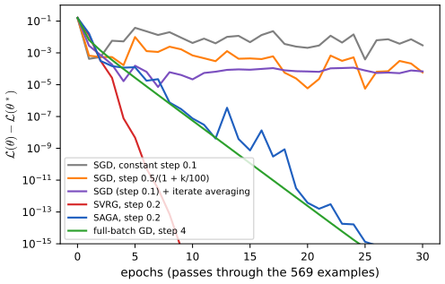
pp. 297–298 For finite sums one can reduce the variance of the gradient estimate rather than of the iterates, and recover a linear rate with a constant step.
SVRG (Johnson and Zhang, 2013) keeps a snapshot \(\tilde\bth\) and its full gradient \(\nabla\cL(\tilde\bth)\), refreshed every epoch, and uses \[ \bm g_t=\nabla\cL_n(\bth_t)-\nabla\cL_n(\tilde\bth)+\nabla\cL(\tilde\bth). \tag{8.66} \] SAGA (Defazio et al., 2014) stores the last gradient \(\bm g_n^{\rm local}\) of every example and their average \(\bm g^{\rm avg}\), and uses \[ \bm g_t=\nabla\cL_n(\bth_t)-\bm g_n^{\rm local}+\bm g^{\rm avg}, \tag{8.67} \] then replaces \(\bm g_n^{\rm local}\) by \(\nabla\cL_n(\bth_t)\) and updates the average: no periodic full pass, at the price of storing \(N\) gradients. Batch normalisation, data augmentation and dropout break the finite-sum structure these methods rely on, which limits their use in deep learning (8.4.5.3).
Filling the gap 8.9: SVRG and SAGA are unbiased, and their variance vanishes at the optimum pp. 297–298
Derivation
Unbiasedness. With \(n\) uniform on \(\{1,\dots,N\}\) and everything else fixed, \(\E_n[\nabla\cL_n(\bth)-\nabla\cL_n(\tilde\bth)]=\nabla\cL(\bth)-\nabla\cL(\tilde\bth)\), so \(\E_n\bm g_t=\nabla\cL(\bth_t)\) for SVRG. For SAGA, \(\E_n[\bm g_n^{\rm local}]=\bm g^{\rm avg}\) by definition of the average, so again \(\E_n\bm g_t=\nabla\cL(\bth_t)\).
Variance. For SVRG, \(\bm g_t-\nabla\cL(\bth_t)=\bm u_n-\E_n\bm u_n\) with \(\bm u_n=\nabla\cL_n(\bth_t)-\nabla\cL_n(\tilde\bth)\), so \[ \E_n\|\bm g_t-\nabla\cL(\bth_t)\|^2\le\E_n\|\bm u_n\|^2\le L_{\max}^2\|\bth_t-\tilde\bth\|^2 \] if every \(\cL_n\) is \(L_{\max}\)-smooth (a variance is at most the second moment). As \(\bth_t\) and \(\tilde\bth\) approach \(\bth^*\) the variance tends to 0, whereas plain SGD keeps the variance \(\frac1N\sum_n\|\nabla\cL_n(\bth^*)\|^2>0\) at the optimum. The same holds for SAGA with \(\tilde\bth\) replaced by the points at which the stored gradients were computed.
Rate (quoted). For \(m\)-strongly convex \(\cL\), \(L\)-smooth \(\cL_n\), step \(\eta<1/(4L)\) and \(K\) inner steps per snapshot, Johnson and Zhang prove \(\E[\cL(\tilde\bth_{s+1})-\cL^*]\le\alpha\,\E[\cL(\tilde\bth_s)-\cL^*]\) with \(\alpha=\frac1{m\eta(1-2L\eta)K}+\frac{2L\eta}{1-2L\eta}<1\) for \(K\) large enough: linear convergence per epoch, like full gradient descent, at the cost of about two example gradients per step plus one full gradient per epoch. Figure 8.S3 shows it. \(\square\)
8.4.6 Preconditioned SGD
pp. 298–299 Preconditioned SGD takes \(\bth_{t+1}=\bth_t-\eta_t\bm M_t^{-1}\bm g_t\) (8.68) with a positive definite \(\bm M_t\), in practice diagonal because noisy Hessians are hard to estimate and full matrices expensive to invert.
8.4.6.1 AdaGrad
p. 299 AdaGrad (Duchi et al., 2011) divides each coordinate by the root of its accumulated squared gradients, \[ \theta_{t+1,d}=\theta_{t,d}-\eta_t\frac{g_{t,d}}{\sqrt{s_{t,d}+\epsilon}},\qquad s_{t,d}=\sum_{i=1}^tg_{i,d}^2, \tag{8.69, 8.70} \] i.e. \(\bm M_t=\diag(\bm s_t+\epsilon)^{1/2}\). Rare features (coordinates with small accumulated gradients) get large steps. The vector form (8.71) puts \(\epsilon\) outside the square root, \(\bm g_t/(\sqrt{\bm s_t}+\epsilon)\), a slightly different but equally common variant.
8.4.6.2 RMSProp and AdaDelta
pp. 299–300 AdaGrad's denominator only grows. RMSProp replaces the sum by an exponentially weighted moving average, \(s_{t+1,d}=\beta s_{t,d}+(1-\beta)g_{t,d}^2\) (8.72), and steps by \(-\eta_t\bm g_t/(\sqrt{\bm s_t}+\epsilon)\) (8.74). Unrolling from \(\bm s_0=\bm 0\), \(s_{t,d}=(1-\beta)\sum_{\tau=1}^{t}\beta^{t-\tau}g_{\tau,d}^2\): the root of an exponentially weighted mean of squares over roughly the last \(1/(1-\beta)\) steps, with weights summing to \(1-\beta^t\); this is the precise meaning of the "RMS" in (8.73), which writes it as an unweighted mean over all steps. AdaDelta (8.75)–(8.76) also tracks the squared updates \(\delta_t\) and multiplies by \(\sqrt{\delta_{t-1}+\epsilon}\), so the update has the units of \(\bth\).
8.4.6.3 Adam
p. 300 Adam (Kingma and Ba, 2015) combines a moving average of gradients (momentum) with RMSProp: \[ \bm m_t=\beta_1\bm m_{t-1}+(1-\beta_1)\bm g_t,\qquad\bm s_t=\beta_2\bm s_{t-1}+(1-\beta_2)\bm g_t^2,\qquad\bth_t=\bth_{t-1}-\eta_t\frac{\hat{\bm m}_t}{\sqrt{\hat{\bm s}_t}+\epsilon}, \tag{8.77–8.79} \] with the bias-corrected moments \[ \hat{\bm m}_t=\bm m_t/(1-\beta_1^t),\qquad\hat{\bm s}_t=\bm s_t/(1-\beta_2^t), \tag{8.80, 8.81} \] and the defaults \(\beta_1=0.9\), \(\beta_2=0.999\), \(\epsilon=10^{-8}\) of the original paper (the book quotes \(10^{-6}\), and writes \(\bth_t\) on both sides of (8.79)).
Filling the gap 8.10: why the bias correction (8.80)–(8.81) divides by \(1-\beta^t\) p. 300
Derivation
From \(\bm m_0=\bm 0\), \(\bm m_t=(1-\beta_1)\sum_{i=1}^t\beta_1^{t-i}\bm g_i\). If the gradients have a common mean, \(\E\bm g_i=\bar{\bm g}\), then \(\E\bm m_t=\bar{\bm g}(1-\beta_1)\sum_{i=1}^t\beta_1^{t-i}=\bar{\bm g}(1-\beta_1^t)\) (a finite geometric sum). So \(\bm m_t\) is biased towards 0 by the factor \(1-\beta_1^t\), large for small \(t\) (\(1-0.999^t\) is still 0.095 at \(t=100\) for the second moment), and \(\hat{\bm m}_t\) is unbiased; the same computation with \(\bm g_i^2\) gives (8.81). For a constant gradient the correction is exact at every step (checked to \(10^{-12}\)). This is the bias-corrected moving average of the book's Section 4.4.2.2 (Chapter 4 notes). \(\square\)
See also (companion): Foundations of Deep Learning, 7.3.3 RMSProp and Adam.
8.4.6.4 Issues with adaptive learning rates
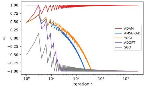
p. 301 Because the effective step \(\eta_0\bm M_t^{-1}\) need not decrease, EWMA methods can fail to converge even on convex problems (Reddi et al., 2018). Remedies include AMSGrad (use the running maximum of \(\bm s_t\)), Padam, Yogi, which replaces \(\bm s_t=\bm s_{t-1}+(1-\beta_2)(\bm g_t^2-\bm s_{t-1})\) (8.82) by \[ \bm s_t=\bm s_{t-1}+(1-\beta_2)\,\bm g_t^2\odot\sgn(\bm g_t^2-\bm s_{t-1}), \tag{8.83} \] so that \(\bm s\) moves by a bounded amount towards \(\bm g_t^2\), and ADOPT (Taniguchi et al., 2024), which normalises the gradient by the previous second moment before averaging, \(\bm m_t=\beta_1\bm m_{t-1}+(1-\beta_1)\bm g_t/\sqrt{\bm s_{t-1}+\epsilon}\), and steps by \(-\eta_t\bm m_t\).
Filling the gap 8.11: a convex problem on which Adam converges to the worst point p. 301
Derivation
Reddi et al. (2018) take the online problem on \(x\in[-1,1]\) with \(f_t(x)=Cx\) when \(t\bmod3=1\) and \(f_t(x)=-x\) otherwise, \(C>2\). Over a cycle the losses sum to \((C-2)x\), minimised at \(x=-1\). Plain projected SGD moves by \(-\eta(C-2)\) per cycle (for slowly varying \(\eta_t\)) and reaches \(-1\).
Now run Adam with \(\beta_1=0\) (no momentum), \(\beta_2=1/(1+C^2)\), no bias correction, steps \(\eta_t=\alpha/\sqrt t\). Take \(C=3\), so \(\beta_2=0.1\). In the periodic regime let \(v_1,v_2,v_3\) be the second-moment values after the gradients \(3,-1,-1\): \(v_1=0.1v_3+0.9\cdot9\), \(v_2=0.1v_1+0.9\), \(v_3=0.1v_2+0.9\). Solving the linear system, \(v_3=1.071/0.999=1.07207\), \(v_2=1.72072\), \(v_1=8.20721\). The three normalised steps are \(3/\sqrt{v_1}=1.04719\) (downwards) and \(1/\sqrt{v_2}=0.76234\), \(1/\sqrt{v_3}=0.96579\) (upwards). Net movement per cycle: \[\eta(0.76234+0.96579-1.04719)=+0.68094\,\eta. \] The large but rare gradient is divided by its own large \(\sqrt v\), while the small frequent gradients are divided by a \(\sqrt v\) that has already decayed: the informative gradient is muted. Since \(\sum\eta_t=\infty\) (and the variation of \(\eta_t\) within a cycle is \(O(t^{-3/2})\), summable), \(x_t\) is driven to the boundary \(+1\), where the average loss is largest.
AMSGrad divides every step by \(\sqrt{\hat v}\) with \(\hat v=\max v\approx8.21\), the same for all three steps, so the net movement per cycle is \(-\eta(3-2)/\sqrt{\hat v}<0\) and \(x_t\to-1\). Yogi's bounded change of \(s\) and ADOPT's normalisation by the previous second moment also restore convergence. Figure 8.S4 shows all of this numerically: after 30,000 steps Adam is at \(x=1.000\), AMSGrad at \(-0.998\), ADOPT at \(-0.997\). \(\square\)
8.4.6.5 Non-diagonal preconditioning matrices
p. 301 Diagonal scalings do not undo correlations between parameters. Full-matrix AdaGrad uses the outer products of past gradients \(\bm G_t=[\bm g_t,\dots,\bm g_1]\) (8.85) and the step \(-\eta\big[(\bm G_t\bm G_t^\T)^{1/2}+\epsilon\bm I\big]^{-1}\bm g_t\); in the notation of (8.68) the preconditioner is \(\bm M_t=(\bm G_t\bm G_t^\T)^{1/2}+\epsilon\bm I\), not its inverse as (8.84) writes. Storing and inverting a \(D\times D\) matrix is too costly for large models; Shampoo uses one block per layer with a Kronecker-factored approximation.
8.5 Constrained optimization
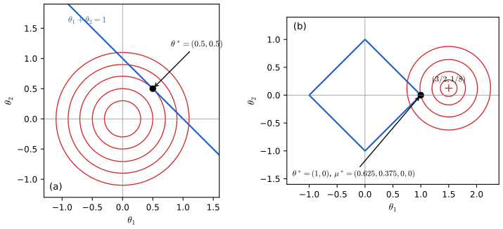
p. 302 The problem is \(\bth^*=\argmin_{\bth\in\mathcal C}\cL(\bth)\) (8.86) with \(\mathcal C=\{\bth:h_i(\bth)=0,\ i\in\mathcal E,\ g_j(\bth)\le0,\ j\in\mathcal I\}\) (8.87). Figure 8.20 shows the two running examples.
See also (companion): Foundations of Deep Learning, Appendix C.1 and its Lagrange multiplier demo.
8.5.1 Lagrange multipliers
pp. 302–303 On the surface \(h(\bth)=0\) the gradient \(\nabla h\) is orthogonal to the surface (8.88); at a constrained minimum \(\nabla\cL\) must be orthogonal to it too, hence parallel to \(\nabla h\) (8.89). This is the stationarity of the Lagrangian \[ L(\bth,\lambda)\triangleq\cL(\bth)+\lambda h(\bth),\qquad\nabla_{\bth,\lambda}L=\bm 0\iff\nabla\cL(\bth)+\lambda\nabla h(\bth)=\bm 0,\ h(\bth)=0, \tag{8.90, 8.91} \] and with several constraints \(L=\cL+\sum_j\lambda_jh_j\) (8.92): \(D+m\) equations in \(D+m\) unknowns. (With this Lagrangian the condition is \(\nabla\cL=-\lambda\nabla h\); the book's (8.89) and (8.91) differ by this sign, which is a matter of convention.)
Result 8.12 (the Lagrange multiplier theorem) pp. 302–303
Let \(\cL,h_1,\dots,h_m\) be continuously differentiable and \(\bth^*\) a local minimiser of \(\cL\) on \(\{\bm h(\bth)=\bm 0\}\) at which \(\nabla h_1(\bth^*),\dots,\nabla h_m(\bth^*)\) are linearly independent (a regularity condition). Then there are unique \(\lambda_1^*,\dots,\lambda_m^*\) with \(\nabla\cL(\bth^*)+\sum_j\lambda_j^*\nabla h_j(\bth^*)=\bm 0\). If \(\cL\) is convex and the \(h_j\) are affine, any such point is a global minimiser.
Proof
Let \(\bm N\) be the \(D\times m\) matrix with columns \(\nabla h_j(\bth^*)\) (full column rank) and \(\bm v\) any vector with \(\bm N^\T\bm v=\bm 0\) (tangent to the surface). Consider \(\bm F(s,\bm u)=\bm h(\bth^*+s\bm v+\bm N\bm u)\) for \(s\in\R\), \(\bm u\in\R^m\). \(\bm F(0,\bm 0)=\bm 0\) and \(\partial\bm F/\partial\bm u(0,\bm 0)=\bm N^\T\bm N\) is invertible, so by the implicit function theorem there is a \(C^1\) function \(\bm u(s)\) with \(\bm u(0)=\bm 0\) and \(\bm F(s,\bm u(s))=\bm 0\) near \(s=0\); differentiating, \(\bm N^\T\bm v+\bm N^\T\bm N\bm u'(0)=\bm 0\), so \(\bm u'(0)=\bm 0\). The curve \(\gamma(s)=\bth^*+s\bm v+\bm N\bm u(s)\) stays on the surface with \(\gamma(0)=\bth^*\), \(\gamma'(0)=\bm v\). Since \(\cL(\gamma(s))\) has a local minimum at \(s=0\), \(\nabla\cL(\bth^*)^\T\bm v=0\). Thus \(\nabla\cL(\bth^*)\) is orthogonal to the null space of \(\bm N^\T\), i.e. it lies in the column space of \(\bm N\): \(\nabla\cL(\bth^*)=-\bm N\bm\lambda^*\), unique because \(\bm N\) has full rank.
Global optimality in the convex case. If \(\cL\) is convex and \(h_j(\bth)=\bm a_j^\T\bth-b_j\), then for any feasible \(\bth\), \[\cL(\bth)=\cL(\bth)+\sum_j\lambda_j^*h_j(\bth)\ge\cL(\bth^*)+\big(\nabla\cL(\bth^*)+\sum_j\lambda_j^*\bm a_j\big)^\T(\bth-\bth^*)+\sum_j\lambda_j^*h_j(\bth^*)=\cL(\bth^*), \] by convexity (the Lagrangian is convex in \(\bth\) whatever the signs of the \(\lambda_j\), since the \(h_j\) are affine) and stationarity. \(\square\)
8.5.1.1 Example: 2d quadratic objective with one linear equality constraint
p. 303 For \(\min\theta_1^2+\theta_2^2\) subject to \(\theta_1+\theta_2=1\), \(L=\theta_1^2+\theta_2^2+\lambda(\theta_1+\theta_2-1)\) (8.93); \(2\theta_1+\lambda=0\), \(2\theta_2+\lambda=0\), \(\theta_1+\theta_2=1\) (8.94)–(8.96) give \(\bth^*=(0.5,0.5)\) and \(\lambda^*=-1\), a global minimum by Result 8.12.
8.5.2 The KKT conditions
pp. 304–305 An inequality \(g(\bth)\le0\) could be imposed by the infinite penalty \(\infty\,\mathbb I(g(\bth)>0)\) (8.97); instead use \(L(\bth,\mu)=\cL(\bth)+\mu g(\bth)\) with \(\mu\ge0\) (8.98), because \[ \max_{\mu\ge0}L(\bth,\mu)=\begin{cases}\infty&g(\bth)>0,\\ \cL(\bth)&g(\bth)\le0,\end{cases} \tag{8.99} \] (if \(g>0\), \(\mu g\) is unbounded; if \(g\le0\), the maximum is at \(\mu=0\)). So the problem is \(\min_{\bth}\max_{\mu\ge0}L\) (8.100), and with all constraints \(\min_{\bth}\max_{\bm\mu\ge0,\bm\lambda}L(\bth,\bm\mu,\bm\lambda)\), \(L=\cL+\sum_i\mu_ig_i+\sum_j\lambda_jh_j\) (8.101)–(8.102). The Karush–Kuhn–Tucker conditions are
- primal feasibility: \(\bm g(\bth^*)\le\bm 0\), \(\bm h(\bth^*)=\bm 0\) (8.103);
- stationarity: \[\nabla\cL(\bth^*)+\sum_i\mu_i\nabla g_i(\bth^*)+\sum_j\lambda_j\nabla h_j(\bth^*)=\bm 0\] (8.104);
- dual feasibility: \(\bm\mu\ge\bm 0\) (8.105);
- complementary slackness: \(\bm\mu\odot\bm g(\bth^*)=\bm 0\) (8.106).
An active constraint (\(g_i=0\)) behaves like an equality, and stationarity then says \(\nabla\cL=-\mu_i\nabla g_i\) with \(\mu_i\ge0\): the objective's descent direction \(-\nabla\cL\) points out of the feasible set, along the outward normal \(\nabla g_i\). An inactive one (\(g_i<0\)) has \(\mu_i=0\).
Result 8.13 (when the KKT conditions are sufficient, and when necessary) p. 305
(a) Sufficiency. If \(\cL\) and the \(g_i\) are convex and differentiable and the \(h_j\) affine, any \((\bth^*,\bm\mu,\bm\lambda)\) satisfying (8.103)–(8.106) makes \(\bth^*\) a global minimiser. (b) Necessity needs a constraint qualification: if the constraints are affine (linear and quadratic programs), or convex with a strictly feasible point (Slater's condition), or have linearly independent active gradients, then every local minimiser has KKT multipliers. Without one it can fail: for \(\min\theta\) subject to \(\theta^2\le0\) the only feasible point \(\theta^*=0\) is optimal, but \(1+\mu\cdot2\theta^*=1\ne0\) for every \(\mu\).
Proof
(a) For feasible \(\bth\), since \(\bm\mu\ge\bm0\), \(\bm g(\bth)\le\bm 0\) and \(\bm h(\bth)=\bm0\), \[ \cL(\bth)\ge L(\bth,\bm\mu,\bm\lambda)\ge L(\bth^*,\bm\mu,\bm\lambda)+\nabla_{\bth}L(\bth^*,\bm\mu,\bm\lambda)^\T(\bth-\bth^*)=L(\bth^*,\bm\mu,\bm\lambda)=\cL(\bth^*). \] The second inequality holds because \(L(\cdot,\bm\mu,\bm\lambda)\) is convex (a non-negative combination of convex functions plus affine ones), the equality after it is stationarity, and the last equality is complementary slackness with \(\bm h(\bth^*)=\bm0\).
(b), affine constraints \(\bm a_i^\T\bth\le b_i\), \(\bm c_j^\T\bth=d_j\). Let \(S\) be the active set at a local minimiser \(\bth^*\). If a direction \(\bm d\) had \(\bm a_i^\T\bm d\le0\) (\(i\in S\)), \(\bm c_j^\T\bm d=0\) and \(\nabla\cL(\bth^*)^\T\bm d<0\), then \(\bth^*+\eta\bm d\) would be feasible for small \(\eta>0\) (inactive constraints have slack, active ones and equalities are kept by linearity) and better (Section 8.2.1), a contradiction. So the linear system has no solution, and by Farkas' lemma (a theorem of the alternative for linear inequalities, e.g. Boyd and Vandenberghe 2004, Section 5.8.3) there exist \(\mu_i\ge0\) (\(i\in S\)) and \(\lambda_j\) with \(\nabla\cL(\bth^*)+\sum_{i\in S}\mu_i\bm a_i+\sum_j\lambda_j\bm c_j=\bm0\). Setting \(\mu_i=0\) off \(S\) gives (8.103)–(8.106). The Slater and independence cases are proved in Boyd and Vandenberghe (2004, Section 5.5.3) and Nocedal and Wright (2006, Theorem 12.1). \(\square\)
See also (companion): Foundations of Deep Learning, Appendix C.2 the KKT conditions; SVMs in Bayesian and Probabilistic ML, 7.1 use exactly these conditions.
8.5.3 Linear programming
pp. 305–306 A linear program in standard form is \[ \min_{\bth}\bm c^\T\bth\quad\text{s.t.}\quad\bm A\bth\le\bm b,\ \bth\ge\bm 0; \tag{8.107} \] its feasible set is a convex polytope (an intersection of half-spaces). Either the feasible set is empty (the problem is infeasible), or the objective is unbounded below on it (unbounded), or an optimum exists, and then one is attained at a vertex. (The book describes the second case as "infeasible", which is the name of the first.)
Filling the gap 8.12: an optimum of a linear program is attained at a vertex p. 306
Derivation
Suppose the feasible set \(P\) is a nonempty bounded polytope. By the Minkowski (Krein–Milman) theorem for polytopes, \(P\) is the convex hull of its finitely many vertices \(\bm v_1,\dots,\bm v_K\). Any \(\bth\in P\) is \(\sum_k\alpha_k\bm v_k\) with \(\alpha_k\ge0\), \(\sum\alpha_k=1\), so \(\bm c^\T\bth=\sum_k\alpha_k\bm c^\T\bm v_k\ge\min_k\bm c^\T\bm v_k\): the best vertex is optimal. If the optimum is unique it is that vertex; if several vertices tie, the whole face they span is optimal (the level line is parallel to a face). For unbounded \(P\) with \(\bm c^\T\bth\) bounded below the conclusion still holds when \(P\) contains no line, which \(\bth\ge\bm0\) guarantees (the fundamental theorem of linear programming; see Bertsekas 2016). The simplex method of Figure 8.21 walks along edges from vertex to vertex, never increasing the objective; with Bland's anti-cycling rule it terminates. The code's implementation reaches \((3.2,2.4)\) in 3 pivots and agrees with scipy's linear programming solver; an empty set and an unbounded objective are reported by that solver as two different failure codes. \(\square\)
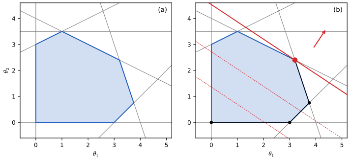
p. 306 The simplex method can take exponentially many steps in the worst case but is usually fast; interior-point methods are polynomial. LPs appear in robust (\(\ell_1\)) regression (Section 11.6.1.1 of the book) and in inference for graphical models.
8.5.4 Quadratic programming
pp. 306–307 A quadratic program is \[ \min_{\bth}\tfrac12\bth^\T\bm H\bth+\bm c^\T\bth\quad\text{s.t.}\quad\bm A\bth\le\bm b,\ \bm C\bth=\bm d, \tag{8.108} \] convex when \(\bm H\succeq0\); then by Result 8.13 the KKT conditions are necessary and sufficient.
8.5.4.1 Example: 2d quadratic objective with linear inequality constraints
pp. 306–307 Minimise \[(\theta_1-\frac32)^2+(\theta_2-\frac18)^2=\frac12\bth^\T\bm H\bth+\bm c^\T\bth+\const\] with \(\bm H=2\bm I\), \(\bm c=-(3,\frac14)\) (8.109), subject to \(|\theta_1|+|\theta_2|\le1\) (8.110), i.e. the four rows \(\theta_1+\theta_2\le1\), \(\theta_1-\theta_2\le1\), \(-\theta_1+\theta_2\le1\), \(-\theta_1-\theta_2\le1\) (8.111)–(8.113). The centre lies outside the diamond, to the right, so constraints 3 and 4 are inactive and \(\mu_3=\mu_4=0\). Stationarity \(\bm H\bth+\bm c+\bm A^\T\bm\mu=\bm0\) (8.114) on the active rows 1, 2 gives the system (8.115), with solution \[ \bth^*=(1,0)^\T,\qquad\bm\mu^*=(0.625,0.375,0,0)^\T. \tag{8.116} \]
Filling the gap 8.13: checking every KKT condition for (8.116), and why the active set is right p. 307
Derivation
With rows 1 and 2 active, \(\theta_1+\theta_2=1\) and \(\theta_1-\theta_2=1\) give \(\bth=(1,0)\). Stationarity reads \(2\theta_1-3+\mu_1+\mu_2=0\) and \(2\theta_2-\frac14+\mu_1-\mu_2=0\), i.e. \(\mu_1+\mu_2=1\), \(\mu_1-\mu_2=\frac14\), so \(\mu_1=0.625\), \(\mu_2=0.375\). Now all four conditions: feasibility, \(\bm A\bth^*=(1,1,-1,-1)\le\bm 1\); dual feasibility, \(\bm\mu^*\ge\bm0\); complementary slackness, rows 1–2 have zero slack and rows 3–4 zero multipliers; stationarity, by construction. Since \(\bm H=2\bm I\succ0\), Result 8.13(a) makes \((1,0)\) the unique global minimiser. The guess of the active set matters: had we assumed only row 1 active, the KKT system would give \(\bth=(1.1875,-0.1875)\) with \(\mu_1=0.625\), which violates row 2; the code's solver tries the active sets in turn and keeps the one passing all checks, and the result agrees with a general-purpose constrained solver. Geometrically, \[-\nabla\cL(\bth^*)=(1,0.25)=0.625(1,1)+0.375(1,-1)\] lies in the cone of the two outward normals at the vertex, which is the picture the demonstration draws. \(\square\)
p. 307 Applications. The lasso, \(\min\|\bm X\bm w-\bm y\|^2+\lambda\|\bm w\|_1\), is a QP after splitting \(\bm w=\bm w^+-\bm w^-\) with \(\bm w^\pm\ge\bm0\) and replacing \(\|\bm w\|_1\) by \(\bm1^\T(\bm w^++\bm w^-)\): at an optimum \(w_d^+w_d^-=0\) (otherwise subtracting \(\min(w_d^+,w_d^-)\) from both lowers the penalty and leaves the fit unchanged), so the two problems agree. SVMs are QPs (Section 17.3 of the book).
8.5.5 Mixed integer linear programming *
pp. 307–308 An integer linear program adds \(\bth\in\mathbb Z^D\) to (8.107) (8.117); with only some integer variables it is a mixed integer program (MIP). MIPs are NP-hard in general and are solved by branch and bound on LP relaxations; they are used for routing, scheduling and for verifying neural networks.
8.6 Proximal gradient method *
p. 308 For a composite objective \(\cL=\cL_s+\cL_r\) (8.118) with \(\cL_s\) smooth and \(\cL_r\) convex but possibly non-smooth, the proximal gradient method takes a gradient step on \(\cL_s\) and then a proximal step on \(\cL_r\): \[ \bth_{t+1}=\prox_{\eta_t\cL_r}\big(\bth_t-\eta_t\nabla\cL_s(\bth_t)\big),\qquad\prox_{\eta\cL_r}(\bth)\triangleq\argmin_{\bm z}\Big\{\cL_r(\bm z)+\frac1{2\eta}\|\bm z-\bth\|^2\Big\}. \tag{8.119, 8.120} \] Equivalently the prox minimises \(\cL_r\) over a ball \(\|\bm z-\bth\|\le\rho\) (8.121), with \(\rho=\|\prox_{\eta\cL_r}(\bth)-\bth\|\), a radius that depends on \(\bth\) as well as \(\eta\): if a point \(\bm z\) of that ball had \(\cL_r(\bm z)<\cL_r(\bm z^*)\), it would also have a smaller value of the objective in (8.120).
Result 8.14 (proximal operators used in this section) pp. 308–311
- For convex, closed \(\cL_r\) the prox exists and is unique: the objective in (8.120) is \(\frac1\eta\)-strongly convex.
- The prox of the indicator \(I_{\mathcal C}\) of a closed convex set (8.124) is the Euclidean projection \(\proj_{\mathcal C}(\bth)=\argmin_{\bth'\in\mathcal C}\|\bth'-\bth\|\) (8.125), for every \(\eta\).
- For a box \(\{\bm l\le\bth\le\bm u\}\) the projection clips each coordinate (8.126); for \(\bth\ge\bm0\) it is \(\bth_+\) (8.127).
- For \(\cL_r=\lambda\|\bth\|_1\) the prox with \(\eta=1\) is soft thresholding, \[ \prox_{\lambda\|\cdot\|_1}(\bth)=\sgn(\bth)\odot(|\bth|-\lambda)_+. \tag{8.133–8.135} \]
- The projection on the \(\ell_1\) ball \(\{\|\bth\|_1\le r\}\) is soft thresholding \(\sgn(\bth)(|\bth|-\tau)_+\) at the level \(\tau\ge0\) for which the result has norm \(r\) (\(\tau=0\) if \(\bth\) is already inside).
Proof
1. A strongly convex closed function is coercive, so a minimiser exists, and strong convexity makes it unique (Filling the gap 8.1). 2. \(I_{\mathcal C}(\bm z)+\frac1{2\eta}\|\bm z-\bth\|^2\) is infinite off \(\mathcal C\) and equals \(\frac1{2\eta}\|\bm z-\bth\|^2\) on it. 3. \(\|\bm z-\bth\|^2=\sum_d(z_d-\theta_d)^2\) and the constraints act on separate coordinates, so each \(z_d\) minimises \((z_d-\theta_d)^2\) over \([l_d,u_d]\): the clipped value. 4. The problem separates; in one coordinate, by Filling the gap 8.3, \(0\in\lambda\,\partial|z|+z-\theta\). If \(z>0\) this says \(z=\theta-\lambda\), possible iff \(\theta>\lambda\); if \(z<0\), \(z=\theta+\lambda\), possible iff \(\theta<-\lambda\); \(z=0\) works iff \(\theta\in[-\lambda,\lambda]\). The three cases partition the line, giving (8.133). (The book's (8.132) says "with \(\eta=1\)" but is the case \(\eta=\lambda\) of (8.120) applied to \(|z|\), which is the same thing.) 5. The Lagrangian of \(\min\frac12\|\bm z-\bth\|^2\) s.t. \(\|\bm z\|_1\le r\) is \(\frac12\|\bm z-\bth\|^2+\tau(\|\bm z\|_1-r)\); for fixed \(\tau\) its minimiser is soft thresholding at \(\tau\) (part 4), and complementary slackness picks \(\tau=0\) inside or \(\|\bm z\|_1=r\) on the boundary; \(\tau\) is found by sorting \(|\theta_d|\) (Duchi et al., 2008). \(\square\)
Result 8.15 (rates of proximal gradient descent (ISTA) and its accelerated version (FISTA))
Let \(F=\cL_s+\cL_r\) with \(\cL_s\) convex and \(L\)-smooth, \(\cL_r\) convex and closed, and \(\bth^*\) a minimiser. (a) ISTA, \(\bth_{k+1}=\prox_{\cL_r/L}(\bth_k-\frac1L\nabla\cL_s(\bth_k))\), decreases \(F\) at every step and \(F(\bth_k)-F^*\le\frac{L\|\bth_0-\bth^*\|^2}{2k}\). (b) FISTA (Beck and Teboulle, 2009): \(\bm x_k=p(\bm y_k)\) with \(p\) the ISTA map, \(\bm y_1=\bm x_0\), \(s_1=1\), \(s_{k+1}=\frac12(1+\sqrt{1+4s_k^2})\), \(\bm y_{k+1}=\bm x_k+\frac{s_k-1}{s_{k+1}}(\bm x_k-\bm x_{k-1})\), satisfies \(F(\bm x_k)-F^*\le\frac{2L\|\bm x_0-\bth^*\|^2}{(k+1)^2}\). With \(\cL_r=0\), (a) is Result 8.7(a) and (b) is Nesterov's method (8.35)–(8.36) with \(\beta_k=(s_k-1)/s_{k+1}\).
Proof
Key inequality. For any \(\bm y,\bm z\), let \(\bm y^+=p(\bm y)\) and \(\bm G=L(\bm y-\bm y^+)\). The optimality condition of the prox is \(\bm G-\nabla\cL_s(\bm y)\in\partial\cL_r(\bm y^+)\). Add three inequalities: the descent lemma \[\cL_s(\bm y^+)\le\cL_s(\bm y)+\nabla\cL_s(\bm y)^\T(\bm y^+-\bm y)+\frac L2\|\bm y^+-\bm y\|^2; \] convexity of \(\cL_s\), \(\cL_s(\bm y)\le\cL_s(\bm z)+\nabla\cL_s(\bm y)^\T(\bm y-\bm z)\); and the subgradient inequality \[\cL_r(\bm y^+)\le\cL_r(\bm z)+(\bm G-\nabla\cL_s(\bm y))^\T(\bm y^+-\bm z). \] The \(\nabla\cL_s\) terms cancel and, with \(\bm y^+-\bm y=-\bm G/L\), \[ F(\bm y^+)\le F(\bm z)+\bm G^\T(\bm y-\bm z)-\frac1{2L}\|\bm G\|^2.\qquad(*) \] (a) With \(\bm z=\bm y=\bth_k\): \(F(\bth_{k+1})\le F(\bth_k)-\|\bm G\|^2/(2L)\), monotone. With \(\bm z=\bth^*\): \[F(\bth_{k+1})-F^*\le\bm G^\T(\bth_k-\bth^*)-\frac1{2L}\|\bm G\|^2=\frac L2(\|\bth_k-\bth^*\|^2-\|\bth_{k+1}-\bth^*\|^2). \] Summing and using monotonicity as in Result 8.7, \(k(F(\bth_k)-F^*)\le\frac L2\|\bth_0-\bth^*\|^2\).
(b) Rewrite (*) as \[F(\bm z)-F(p(\bm y))\ge\frac L2\|p(\bm y)-\bm y\|^2+L\langle\bm y-\bm z,p(\bm y)-\bm y\rangle. \] Let \(v_k=F(\bm x_k)-F^*\). At \(\bm y=\bm y_{k+1}\) with \(\bm z=\bm x_k\) and with \(\bm z=\bth^*\): \[ v_k-v_{k+1}\ge\tfrac L2\|\bm x_{k+1}-\bm y_{k+1}\|^2+L\langle\bm y_{k+1}-\bm x_k,\bm x_{k+1}-\bm y_{k+1}\rangle,\qquad -v_{k+1}\ge\tfrac L2\|\bm x_{k+1}-\bm y_{k+1}\|^2+L\langle\bm y_{k+1}-\bth^*,\bm x_{k+1}-\bm y_{k+1}\rangle. \] Multiply the first by \(s_{k+1}-1\ge0\), add the second, multiply by \(s_{k+1}\), and use \(s_{k+1}^2-s_{k+1}=s_k^2\) (the defining recursion): \[ s_k^2v_k-s_{k+1}^2v_{k+1}\ge\tfrac L2\Big(\|s_{k+1}(\bm x_{k+1}-\bm y_{k+1})\|^2+2s_{k+1}\langle\bm x_{k+1}-\bm y_{k+1},\,s_{k+1}\bm y_{k+1}-(s_{k+1}-1)\bm x_k-\bth^*\rangle\Big). \] With \[\|\bm b-\bm a\|^2+2\langle\bm b-\bm a,\bm a-\bm c\rangle=\|\bm b-\bm c\|^2-\|\bm a-\bm c\|^2\] for \(\bm a=s_{k+1}\bm y_{k+1}\), \(\bm b=s_{k+1}\bm x_{k+1}\), \(\bm c=(s_{k+1}-1)\bm x_k+\bth^*\), and \(\bm u_k=s_k\bm x_k-(s_k-1)\bm x_{k-1}-\bth^*\), the definition of \(\bm y_{k+1}\) gives \(\bm a-\bm c=\bm u_k\) and \(\bm b-\bm c=\bm u_{k+1}\). Hence \[s_{k+1}^2v_{k+1}+\frac L2\|\bm u_{k+1}\|^2\le s_k^2v_k+\frac L2\|\bm u_k\|^2\le\dots\le v_1+\frac L2\|\bm x_1-\bth^*\|^2\le\frac L2\|\bm x_0-\bth^*\|^2, \] the last step by (*) at \(\bm y=\bm x_0\), \(\bm z=\bth^*\). Finally \(s_{k+1}\ge s_k+\frac12\) (as \(\sqrt{1+4s^2}\ge2s\)), so \(s_k\ge\frac{k+1}2\) and \(v_k\le\frac{2L\|\bm x_0-\bth^*\|^2}{(k+1)^2}\). \(\square\)
Both bounds were checked at every iteration on the lasso of Figure 8.S5b, whose FISTA solution agrees with scikit-learn's coordinate-descent lasso to \(10^{-6}\).
8.6.1 Projected gradient descent
pp. 308–309 To minimise \(\cL_s\) over a convex set \(\mathcal C\) (8.122), take \(\cL_r=I_{\mathcal C}\) (8.123)–(8.124): the proximal gradient step becomes "gradient step, then project" (Result 8.14). Box constraints clip (8.126), non-negativity takes the positive part (8.127).
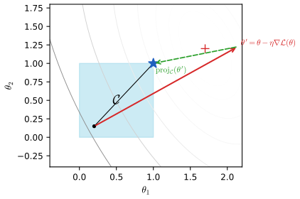
8.6.2 Proximal operator for \(\ell_1\)-norm regularizer
pp. 310–311 The penalty \(\|\bth\|_1=\sum_d|\theta_d|\) (8.128) prefers sparse vectors: \((1,0)\) and \((1/\sqrt2,1/\sqrt2)\) have the same \(\ell_2\) norm (8.129) but \(\ell_1\) norms 1 and \(\sqrt2\) (8.130). For \(\operatorname{NLL}(\bth)+\lambda\|\bth\|_1\) (8.131) the proximal step is soft thresholding (8.132)–(8.135), Result 8.14.4: proximal gradient descent for the lasso is ISTA.
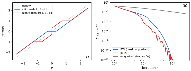
See also (companion): The Elements of Statistical Learning, 3.4.2 the lasso, the l1 and l2 paths demo, and Chapter 11 of the book (Section 11.4) for sparse regression.
8.6.3 Proximal operator for quantization
p. 311 To keep parameters near \(\mathcal C=\{-1,+1\}^D\), penalise the distance \(\cL_r(\bth)=\inf_{\bth_0\in\mathcal C}\|\bth-\bth_0\|_1=\|\bth-\sgn(\bth)\|_1\) (8.136)–(8.137), with quantiser \(q(\bth)=\sgn(\bth)\) (8.138). BinaryConnect uses the straight-through estimator: evaluate the gradient at \(q(\bth_t)\) and update \(\bth_t\) (8.139)–(8.140). ProxQuant takes a proximal step instead (8.141), with \[ \prox_{\lambda\cL_r}(\bth)=\sgn(\bth)+\sgn(\bth-\sgn(\bth))\odot(|\bth-\sgn(\bth)|-\lambda)_+. \tag{8.143} \]
Filling the gap 8.14: deriving the quantisation prox (8.143) p. 311
Derivation
The problem separates over coordinates: minimise \(\phi(z)=\lambda|z-\sgn(z)|+\frac12(z-\theta)^2\). Take \(\theta>0\). For any \(z<0\), its mirror \(-z>0\) has the same penalty (\(|-z-1|=|z+1|\)) and a strictly smaller quadratic term (\((-z-\theta)^2<(z-\theta)^2\) since \(z\theta<0\)); so the minimiser has \(z\ge0\), where \(\phi(z)=\lambda|z-1|+\frac12(z-\theta)^2\). This is the soft-thresholding problem in the variable \(z-1\) with data \(\theta-1\), whose solution is \(z=1+\sgn(\theta-1)(|\theta-1|-\lambda)_+\), and it is non-negative (if \(\theta-1<-\lambda\) it equals \(\theta+\lambda>0\)). This is (8.143) with \(\sgn(\theta)=1\); \(\theta<0\) is symmetric. At \(\theta=0\) the two signs tie: \(\cL_r\) is not convex, and its prox can be set-valued; (8.143) picks \(\sgn(0)=+1\). The formula agrees with a grid minimisation of \(\phi\) to \(2\times10^{-16}\) at 40 test points (Figure 8.S5a). \(\square\)
8.6.4 Incremental (online) proximal methods
p. 311 For sums of per-example losses the proximal step can be applied one example at a time, an online method; Kalman-filter interpretations give a probabilistic view.
8.7 Bound optimization *
8.7.1 The general algorithm
p. 312 To maximise \(\ell(\bth)\), an MM (minorise–maximise) algorithm builds a surrogate \(Q(\bth,\bth_t)\le\ell(\bth)\) with \(Q(\bth_t,\bth_t)=\ell(\bth_t)\) and sets \(\bth_{t+1}=\argmax_{\bth}Q(\bth,\bth_t)\) (8.144). Then \[ \ell(\bth_{t+1})\ge Q(\bth_{t+1},\bth_t)\ge Q(\bth_t,\bth_t)=\ell(\bth_t), \tag{8.145} \] monotone ascent: a decrease signals a bug. Unlike Newton's quadratic approximation, a quadratic lower bound can never overshoot (Figure 8.24).
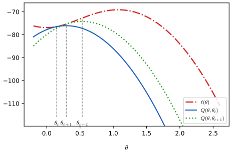
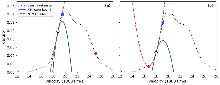
Filling the gap 8.15: mean shift is an MM algorithm (Figure 8.24) p. 313
Derivation
Let \(\hat p(x)=\frac1n\sum_i\kappa\big(u_i(x)\big)\) with \(u_i(x)=(x-x_i)^2/h^2\) and the Gaussian profile \(\kappa(u)=c\,e^{-u/2}\), which is convex in \(u\). A convex function lies above its tangents: \[\kappa(u)\ge\kappa(u_0)+\kappa'(u_0)(u-u_0)=\kappa(u_0)\big(1-\frac12(u-u_0)\big). \] Applying this to each term at \(u_{i0}=u_i(x_0)\), \[ \hat p(x)\ge Q(x,x_0)=\frac1n\sum_iw_i\Big(1-\tfrac12\big(u_i(x)-u_i(x_0)\big)\Big),\qquad w_i=\kappa(u_i(x_0)), \] with equality at \(x=x_0\): a minoriser. \(Q\) is a concave quadratic in \(x\) (the \(u_i\) are convex quadratics with positive weights), maximised where \(\sum_iw_i(x-x_i)=0\), i.e. at the weighted mean \(x_1=\sum_iw_ix_i/\sum_iw_i\): the mean-shift update. By (8.145) every mean-shift step increases \(\hat p\) (Fashing and Tomasi, 2005). Newton's step \(x_0-\hat p'(x_0)/\hat p''(x_0)\) uses the local curvature instead: where \(\hat p''>0\) it seeks a minimum, and where \(\hat p''\) is slightly negative it jumps far. All of this was checked numerically at four starting points. \(\square\)
8.7.2 The EM algorithm
pp. 312–315 EM (Dempster, Laird and Rubin, 1977) is the MM algorithm for latent-variable models. For \(\ell(\bth)=\sum_n\log\sum_{\bm z_n}p(\bm y_n,\bm z_n\given\bth)\) (8.146), any distributions \(q_n\) give, by Jensen's inequality, the evidence lower bound \[ \ell(\bth)\ge\sum_n\sum_{\bm z_n}q_n(\bm z_n)\log\frac{p(\bm y_n,\bm z_n\given\bth)}{q_n(\bm z_n)}=\sum_n\Big(\E_{q_n}[\log p(\bm y_n,\bm z_n\given\bth)]+\mathbb H(q_n)\Big)=\text{Ł}(\bth,q_{1:N}) \tag{8.147–8.150} \] and each term equals \(\log p(\bm y_n\given\bth)-D_{\rm KL}(q_n\|p(\bm z_n\given\bm y_n,\bth))\) (8.151)–(8.154). The E step sets \(q_n=p(\bm z_n\given\bm y_n,\bth_t)\), making the bound tight (8.155); \(Q(\bth,\bth_t)=\text{Ł}(\bth,\{p(\bm z_n\given\bm y_n,\bth_t)\})\) (8.156) is then a minoriser in the sense of Section 8.7.1. The M step maximises the expected complete-data log-likelihood \(\ell_t(\bth)=\sum_n\E_{q_n^t}[\log p(\bm y_n,\bm z_n\given\bth)]\) (8.157), (8.159). Approximate posteriors give variational EM.
See also (companion): Bayesian and Probabilistic ML, 9.4 the EM algorithm in general (the decomposition and monotonicity proved in full), its EM bound demo, and Chapter 6 notes for the KL divergence.
Filling the gap 8.16: the M step for exponential families is moment matching p. 315, (8.158)
Derivation
If \[p(\bm y,\bm z\given\bth)=h(\bm y,\bm z)\exp(\bth^\T\mathcal T(\bm y,\bm z)-A(\bth)), \] then up to a constant \(\ell_t(\bth)=\bth^\T\sum_n\E[\mathcal T(\bm y_n,\bm z_n)]-NA(\bth)\) (8.158). Since \(A\) is convex (its Hessian is the covariance of \(\mathcal T\)), \(\ell_t\) is concave, and its maximiser solves \(\nabla A(\bth)=\frac1N\sum_n\E[\mathcal T(\bm y_n,\bm z_n)]\). As \(\nabla A(\bth)=\E_{\bth}[\mathcal T]\), the M step chooses the parameter whose expected sufficient statistics equal the average expected sufficient statistics from the E step: moment matching. So the E step only needs to return \(\sum_n\E[\mathcal T(\bm y_n,\bm z_n)]\). \(\square\)
8.7.3 Example: EM for a GMM
pp. 315–316 E step: the responsibilities \[ r_{nk}^{(t)}=\frac{\pi_k^{(t)}\N(\bm y_n\given\bm\mu_k^{(t)},\bm\Sigma_k^{(t)})}{\sum_{k'}\pi_{k'}^{(t)}\N(\bm y_n\given\bm\mu_{k'}^{(t)},\bm\Sigma_{k'}^{(t)})}. \tag{8.160} \] M step: with \(r_k^{(t)}=\sum_nr_{nk}^{(t)}\), \[ \bm\mu_k^{(t+1)}=\frac{\sum_nr_{nk}^{(t)}\bm y_n}{r_k^{(t)}},\qquad\bm\Sigma_k^{(t+1)}=\frac{\sum_nr_{nk}^{(t)}(\bm y_n-\bm\mu_k^{(t+1)})(\bm y_n-\bm\mu_k^{(t+1)})^\T}{r_k^{(t)}},\qquad\pi_k^{(t+1)}=\frac{r_k^{(t)}}N. \tag{8.165–8.167} \]
Filling the gap 8.17: the GMM M step p. 316, (8.161)–(8.167)
Derivation
With one-hot \(z_{nk}\), \[\log p(\bm y_n,\bm z_n\given\bth)=\sum_kz_{nk}(\log\pi_k+\log\N(\bm y_n\given\bm\mu_k,\bm\Sigma_k)), \] and \(\E[z_{nk}]=r_{nk}\), so \(\ell_t\) is (8.164): a sum of a term in \(\bm\pi\) only and one term per component. Weights: maximise \(\sum_kr_k\log\pi_k\) on the simplex; by Gibbs' inequality applied to \((r_k/N)_k\) and \(\bm\pi\) (as in Chapter 4 notes, gap 4.1) the maximiser is \(\pi_k=r_k/N\). Component \(k\): maximise \(\sum_nr_{nk}\log\N(\bm y_n\given\bm\mu_k,\bm\Sigma_k)\), the Gaussian log-likelihood with weights \(r_{nk}\). The gradient in \(\bm\mu_k\) is \(\bm\Sigma_k^{-1}\sum_nr_{nk}(\bm y_n-\bm\mu_k)\), zero at the weighted mean; with the trace trick the gradient in \(\bm\Lambda_k=\bm\Sigma_k^{-1}\) is \(\frac{r_k}2\bm\Sigma_k-\frac12\sum_nr_{nk}(\bm y_n-\bm\mu_k)(\bm y_n-\bm\mu_k)^\T\), zero at the weighted scatter divided by \(r_k\). Global optimality is the unweighted argument of Chapter 4 notes, gap 4.3, with \(N\) replaced by \(r_k\). The second form of (8.166) follows by expanding the outer product and using \(\sum_nr_{nk}\bm y_n=r_k\bm\mu_k\). The M step was confirmed against a numerical maximisation of \(\ell_t\). \(\square\)
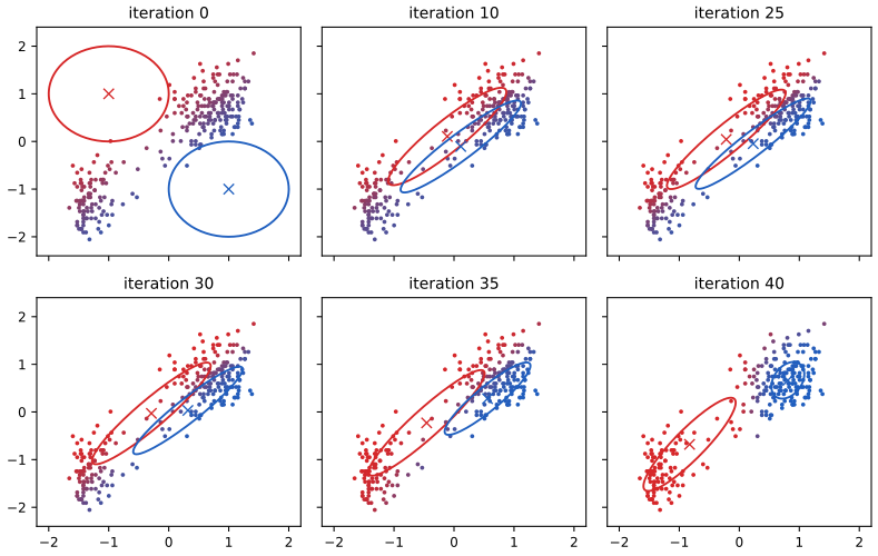
See also (companion): Bayesian and Probabilistic ML, 9.2.2 EM for Gaussian mixtures, Foundations of Deep Learning, 15.3.1, and its EM and ELBO demo.
8.7.3.4 MAP estimation
pp. 317–318 The GMM likelihood is unbounded: centring a component on one data point and letting its variance shrink sends that term to infinity (8.168), the collapsing-variance problem (Figure 8.26a). MAP estimation fixes it. The E step is unchanged; the M step maximises \(\ell_t(\bth)+\log p(\bm\pi)+\sum_k\log p(\bth_k)\) (8.169). With a Dirichlet prior \(\operatorname{Dir}(\bm\alpha)\), \[ \tilde\pi_k=\frac{r_k+\alpha_k-1}{N+\sum_k\alpha_k-K}, \tag{8.170} \] and with a normal-inverse-Wishart prior with \(\breve\kappa=0\) (no prior on the means) and \(\breve\nu,\breve{\bm S}\), the means are unchanged (8.172) and \[ \tilde{\bm\Sigma}_k=\frac{\breve{\bm S}+r_k\hat{\bm\Sigma}_k}{\breve\nu+r_k+D+2}, \tag{8.173, corrected} \] where \(\hat{\bm\Sigma}_k\) is the MLE (8.166). The book's (8.173) has \(\breve{\bm S}+\hat{\bm\Sigma}_k\) in the numerator, which is dimensionally inconsistent (a covariance added to a scatter-type matrix) and shrinks to \(\bm 0\) as \(r_k\) grows. A common choice is \(\breve{\bm S}=K^{-2/D}\diag(s_1^2,\dots,s_D^2)\) (8.174) with the pooled variances \(s_d^2\), and the weakest proper \(\breve\nu=D+2\).
Filling the gap 8.18: the singularity, and the MAP updates (8.170) and (8.173) pp. 317–318
Derivation
Unbounded likelihood. Take \(K\ge2\), \(\bm\Sigma_k=\sigma_k^2\bm I\), \(\bm\mu_1=\bm y_1\), and fix all other parameters. Every factor \(p(\bm y_n\given\bth)\ge\pi_2\N(\bm y_n\given\bm\mu_2,\bm\Sigma_2)\) is bounded below by a positive constant, and \(p(\bm y_1\given\bth)\ge\pi_1(2\pi\sigma_1^2)^{-D/2}\) (in \(D\) dimensions; (8.168) shows \(D=1\)). As \(\sigma_1\to0\) the likelihood tends to infinity, so no MLE exists; EM may approach such a point, where \(\bm\Sigma_1\) becomes singular.
Weights (8.170). The terms in \(\bm\pi\) are \(\sum_k(r_k+\alpha_k-1)\log\pi_k\). If all \(r_k+\alpha_k-1>0\), the Gibbs argument of gap 8.17 with weights proportional to \(r_k+\alpha_k-1\) gives \(\tilde\pi_k\propto r_k+\alpha_k-1\); the normaliser is \(\sum_k(r_k+\alpha_k-1)=N+\sum\alpha_k-K\). \(\alpha_k=1\) recovers the MLE.
Covariances (8.173). The NIW log density, as a function of \(\bm\Sigma\) with \(\breve\kappa=0\), contributes \(-\frac{\breve\nu+D+2}2\log|\bm\Sigma|-\frac12\operatorname{tr}(\bm\Sigma^{-1}\breve{\bm S})\) (the inverse-Wishart exponent \(\frac{\breve\nu+D+1}2\) plus \(\frac12\) from the normal factor of the mean). The expected complete-data log-likelihood contributes \(-\frac{r_k}2\log|\bm\Sigma|-\frac12\operatorname{tr}(\bm\Sigma^{-1}\bm S_k)\) with the weighted scatter \(\bm S_k=\sum_nr_{nk}(\bm y_n-\bm\mu_k)(\bm y_n-\bm\mu_k)^\T=r_k\hat{\bm\Sigma}_k\). The sum has the form \(-\frac a2\log|\bm\Sigma|-\frac12\operatorname{tr}(\bm\Sigma^{-1}\bm B)\), maximised at \(\bm\Sigma=\bm B/a\) (gap 8.17), here \(\bm B=\breve{\bm S}+r_k\hat{\bm\Sigma}_k\) and \(a=\breve\nu+r_k+D+2\). A numerical maximisation of the posterior on the Old Faithful responsibilities returns this matrix and not the book's. \(\square\)
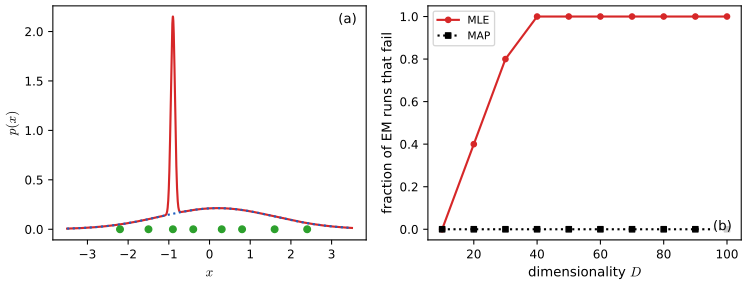
8.7.3.5 Nonconvexity of the NLL
p. 319 The mixture log-likelihood (8.175) is invariant under the \(K!\) relabelings of the components, so a maximiser comes with up to \(K!\) copies (label switching, Figure 8.27). It cannot be concave: the maximisers of a concave function form a convex set, which would contain the average of all relabelings, a point where all components coincide, which is typically far from optimal. Finding a global optimum is NP-hard in general; in practice EM is started from k-means++.
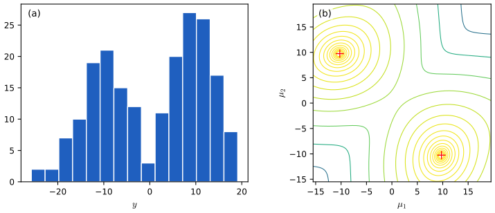
8.8 Blackbox and derivative free optimization
pp. 319–320 When the objective can only be evaluated, as for a validation loss as a function of hyperparameters, gradient methods do not apply. Grid search is the simplest method but scales exponentially with the dimension; random search, Bayesian optimisation and evolutionary methods are treated in the sequel to the book. Unrolling a gradient-based training procedure gives hypergradients in limited settings.
8.9 Exercises
Both exercises of Chapter 8 (Murphy, 2022, p. 320), restated in my own words, with complete solutions (hidden). The dagger marks the book's own flag for exercises with solutions in its solution material; here every solution is worked independently.
Exercise 8.1 † (subderivative of the hinge loss). For \(f(x)=(1-x)_+=\max(0,1-x)\), find \(\partial f(0)\), \(\partial f(1)\) and \(\partial f(2)\).
Solution
\(f\) is convex (a maximum of two affine functions). At \(x=0\) it is differentiable with \(f(x)=1-x\) nearby, so \(\partial f(0)=\{-1\}\) (Filling the gap 8.3). At \(x=2\) it is identically 0 nearby, so \(\partial f(2)=\{0\}\). At the kink \(x=1\), \(g\in\partial f(1)\) iff \((1-z)_+\ge g(z-1)\) for all \(z\). For \(z>1\) this reads \(0\ge g(z-1)\), so \(g\le0\). For \(z<1\) it reads \((1-z)\ge-g(1-z)\), i.e. \((1-z)(1+g)\ge0\), so \(g\ge-1\). Hence \(\partial f(1)=[-1,0]\), the interval between the left and right derivatives. (Checked numerically: every \(g\in[-1,0]\) satisfies (8.13) on a grid and \(g=0.1\) does not.) \(\square\)
Exercise 8.2 (EM for the Student distribution). Derive EM for the maximum likelihood estimate of a multivariate Student distribution \(\mathcal T(\bm x\given\bm\mu,\bm\Sigma,\nu)\), with \(\nu\) known and with \(\nu\) unknown, using its representation as a scale mixture of Gaussians.
Solution
Representation. If \(z\sim\operatorname{Ga}(\frac\nu2,\text{rate}\ \frac\nu2)\) and \(\bm x\given z\sim\N(\bm\mu,\bm\Sigma/z)\), then \(\bm x\sim\mathcal T(\bm\mu,\bm\Sigma,\nu)\): integrating \(z^{D/2}e^{-z\delta/2}\cdot z^{\nu/2-1}e^{-\nu z/2}\) over \(z\), with \(\delta=(\bm x-\bm\mu)^\T\bm\Sigma^{-1}(\bm x-\bm\mu)\), gives a constant times \((\nu+\delta)^{-(\nu+D)/2}\), the Student kernel.
Complete-data log-likelihood with latent \(z_n\): \[ \ell_c=\sum_n\Big[-\tfrac12\log|\bm\Sigma|-\tfrac{z_n}2\delta_n(\bm\mu,\bm\Sigma)+\tfrac\nu2\log\tfrac\nu2-\log\Gamma(\tfrac\nu2)+\tfrac\nu2(\log z_n-z_n)\Big]+(\text{terms in }z_n\text{ only}). \] E step. The same kernel shows \(z_n\given\bm x_n\sim\operatorname{Ga}\big(\frac{\nu+D}2,\text{rate}\ \frac{\nu+\delta_n}2\big)\), so with the current parameters \[ w_n=\E[z_n\given\bm x_n]=\frac{\nu+D}{\nu+\delta_n},\qquad\E[\log z_n\given\bm x_n]=\psi\Big(\frac{\nu+D}2\Big)-\log\frac{\nu+\delta_n}2 . \] M step, \(\nu\) known. Maximise \(\sum_n[-\frac12\log|\bm\Sigma|-\frac{w_n}2\delta_n]\): a weighted Gaussian likelihood with weights \(w_n\) on the quadratic term only, so \[ \bm\mu=\frac{\sum_nw_n\bm x_n}{\sum_nw_n},\qquad\bm\Sigma=\frac1N\sum_nw_n(\bm x_n-\bm\mu)(\bm x_n-\bm\mu)^\T \] (note the divisor \(N\), not \(\sum w_n\)). Outlying points have large \(\delta_n\) and small \(w_n\): EM is iteratively reweighted, and robust.
\(\nu\) unknown. The terms in \(\nu\) are \[N[\frac\nu2\log\frac\nu2-\log\Gamma(\frac\nu2)]+\frac\nu2\sum_n(\E\log z_n-w_n). \] Setting the derivative to zero (an ECM step, Liu and Rubin 1995, holding the E-step quantities fixed): \[ \log\frac\nu2-\psi\Big(\frac\nu2\Big)+1+\frac1N\sum_n\big(\E[\log z_n]-w_n\big)=0 . \] The function \(\log x-\psi(x)\) decreases from \(+\infty\) to 0 on \((0,\infty)\), and \(c=1+\frac1N\sum_n(\E\log z_n-\E z_n)\le0\) because \(\E\log z\le\log\E z\le\E z-1\) (Jensen and \(\log t\le t-1\)); so the equation \(\log\frac\nu2-\psi(\frac\nu2)=-c\) has a unique root when \(c<0\) (and \(\nu=\infty\), the Gaussian, when \(c=0\)), found by one-dimensional root finding. Each EM and ECM step increases the observed-data likelihood (Section 8.7.1).
Computation. On 150 bivariate Gaussian points with 10 gross outliers, the code's EM increases the log-likelihood at every iteration, reaches the same \((\bm\mu,\bm\Sigma)\) as a direct numerical maximisation of the Student likelihood with \(\nu=4\), and the ECM version reaches the joint maximiser with \(\hat\nu=2.32\) (Figure 8.S6). The Student fit ignores the outliers that inflate the Gaussian ellipse. \(\square\)
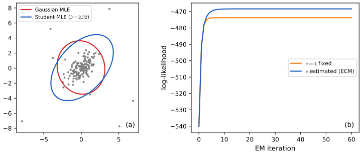
Demonstrations
| Page | What it shows | In the notes |
|---|---|---|
| Line search, Newton, BFGS and trust regions | Constant-step, Armijo and exact-line-search gradient descent, damped Newton, BFGS and a trust-region method on a quadratic of adjustable condition number, the valley (8.19), a Rosenbrock function and a saddle; click to move the start. Presets: 1 step 0.1; 2 step 0.6; 3 exact line search, κ = 30; 4 Rosenbrock; 5 saddle. | 8.2.2, Result 8.6, 8.3 |
| SGD, iterate averaging and variance reduction | SGD with constant and decaying steps and minibatches, Polyak–Ruppert averaging, SVRG, SAGA, Adam and full-batch gradient descent on a 569-term logistic regression. Presets: 1 noise floor; 2 decaying step; 3 averaging; 4 SVRG and SAGA; 5 Adam. | 8.4.3–8.4.6, Result 8.11, gap 8.9 |
| KKT multipliers, projections and proximal steps | A quadratic over an \(\ell_1\) ball, a box or a line, or with an \(\ell_1\) penalty: exact solution, multipliers, KKT residuals, the balance of forces at the solution, and projected or proximal gradient descent. Presets: 1 the book's QP; 2 equality; 3 nothing active; 4 soft thresholding; 5 tilted box. | 8.5, gap 8.13, 8.6 |
The Python code that produces every figure of this page is code/ch08_optimization.py (see the code index). Companion demos: step sizes and momentum, optimiser paths, Lagrange multipliers, the EM bound.
Notes on the book
Points where the book is imprecise or wrong
- (8.19) is not convex. Section 8.2.2.1 calls it convex and says the oscillation of Figure 8.11b happens "even though this is a convex problem". Its Hessian at \((0,1)\) is \(\diag(-1,1)\), and \[\cL(0,1)=1>0.906=\frac12(\cL(-0.5,1)+\cL(0.5,1))\] violates (8.7). The oscillation is explained by (8.20) applied to the Hessian at the minimum (\(\eta=0.6>2/5.83\)).
- Section 8.1.1.1, saddles. "At a saddle point, the eigenvalues of the Hessian will be both positive and negative" is sufficient but not necessary: \(\theta_1^2+\theta_2^3\) has a saddle at the origin with Hessian \(\diag(2,0)\) (Result 8.1).
- (8.18). The text speaks of the angle between \(\bm d\) and \(-\bm g_t\) being below \(90^\circ\), but the formula \(\|\bm d\|\|\bm g_t\|\cos\vartheta<0\) uses the angle between \(\bm d\) and \(\bm g_t\), which must exceed \(90^\circ\).
- Section 8.2.3. A linear rate for "certain convex problems, with a gradient with bounded Lipschitz constant" needs strong convexity or a Polyak–Łojasiewicz condition; \(\theta^4\) is convex and smooth near its minimum, and gradient descent on it is sublinear (Result 8.7).
- (8.47). The curvature condition should read \(\bm d_t^\T\nabla\cL(\bth_t+\eta\bm d_t)\ge c_2\bm d_t^\T\nabla\cL(\bth_t)\): the book's left side is a vector and its right side carries an extra \(\eta\).
- (8.51). Adding \(\lambda\|\bm\delta\|_2^2\) to the model gives the minimiser \(-(\bm H+2\lambda\bm I)^{-1}\bm g\), not (8.52); the penalty should be \(\frac\lambda2\|\bm\delta\|^2\) (checked numerically).
- (8.61), Robbins–Monro conditions. The classical conditions are \(\sum_t\eta_t=\infty\) and \(\sum_t\eta_t^2<\infty\). The ratio condition stated is a different one (it controls the averaged iterate in the convex case, Result 8.11), and the recommended square-root schedule satisfies it but violates \(\sum\eta_t^2<\infty\).
- (8.69) and (8.71). The first puts \(\epsilon\) inside the square root, the second outside; only the first matches \(\bm M_t=\diag(\bm s_t+\epsilon)^{1/2}\).
- (8.73). With the moving average (8.72), \(\sqrt{s_{t,d}}\) is an exponentially weighted root mean square, not the unweighted \(\sqrt{\frac1t\sum_{\tau\le t}g_{\tau,d}^2}\).
- (8.79) and the Adam defaults. The update should read \(\bth_t=\bth_{t-1}-\dots\); Kingma and Ba's default is \(\epsilon=10^{-8}\), not \(10^{-6}\).
- (8.84). With the update (8.68), \(\bth-\eta\bm M^{-1}\bm g\), full-matrix AdaGrad needs \(\bm M_t=(\bm G_t\bm G_t^\T)^{1/2}+\epsilon\bm I\); the book defines \(\bm M_t\) as the inverse of this, which would multiply the gradient by the root of its outer products. The line after (8.85) also writes \(\bm g_i=\nabla\psi c(\psi_i)\), a leftover of other notation.
- (8.89) against (8.91). Stationarity of \(\cL+\lambda h\) gives \(\nabla\cL=-\lambda\nabla h\), not \(\lambda\nabla h=\nabla\cL\); the same sign slip occurs in the explanation of complementary slackness ("\(\nabla\cL=\mu\nabla g\)"), which must be \(\nabla\cL=-\mu\nabla g\) with \(\mu\ge0\) to agree with (8.104).
- Section 8.5.2, necessity of KKT. The conditions are necessary only under a constraint qualification; \(\min\theta\) s.t. \(\theta^2\le0\) has no KKT multiplier (Result 8.13).
- Section 8.5.3. "There may also be no optima inside the feasible set; in this case, the problem is said to be infeasible": infeasible means the feasible set is empty; a nonempty set on which the objective has no minimum makes the problem unbounded.
- (8.121). The radius \(\rho\) depends on \(\bth\) as well as on \(\eta\); and (8.132) says "with \(\eta=1\)" for what is the case \(\eta=\lambda\) applied to \(|z|\).
- (8.168)–(8.169). In \(D\) dimensions the normaliser is \((2\pi\sigma_k^2)^{-D/2}\); in (8.169) \(\log\pi_{nk}\) should be \(\log\pi_k\).
- (8.173). The MAP covariance is \((\breve{\bm S}+r_k\hat{\bm\Sigma}_k)/(\breve\nu+r_k+D+2)\); the book omits the factor \(r_k\) (gap 8.18, confirmed by numerical maximisation of the posterior).
- Figure 8.7. The caption says the non-smooth function has "a discontinuity at the origin"; the function drawn, \(|x|\)-shaped, is continuous, and it is its derivative that jumps.
References
- Murphy, K. P. (2022). Probabilistic Machine Learning: An Introduction. MIT Press, Cambridge, MA. Chapter 8, pp. 275–320. probml.github.io/pml-book/book1.html.
- Beck, A. and Teboulle, M. (2009). A fast iterative shrinkage-thresholding algorithm for linear inverse problems. SIAM Journal on Imaging Sciences, 2(1), 183–202.
- Bertsekas, D. P. (2016). Nonlinear Programming, 3rd edition. Athena Scientific, Belmont, MA.
- Boyd, S. and Vandenberghe, L. (2004). Convex Optimization. Cambridge University Press.
- Defazio, A., Bach, F. and Lacoste-Julien, S. (2014). SAGA: a fast incremental gradient method with support for non-strongly convex composite objectives. Advances in Neural Information Processing Systems 27.
- Dempster, A. P., Laird, N. M. and Rubin, D. B. (1977). Maximum likelihood from incomplete data via the EM algorithm. Journal of the Royal Statistical Society, Series B, 39(1), 1–38.
- Duchi, J., Hazan, E. and Singer, Y. (2011). Adaptive subgradient methods for online learning and stochastic optimization. Journal of Machine Learning Research, 12, 2121–2159.
- Duchi, J., Shalev-Shwartz, S., Singer, Y. and Chandra, T. (2008). Efficient projections onto the l1-ball for learning in high dimensions. Proceedings of the 25th International Conference on Machine Learning.
- Fashing, M. and Tomasi, C. (2005). Mean shift is a bound optimization. IEEE Transactions on Pattern Analysis and Machine Intelligence, 27(3), 471–474.
- Fraley, C. and Raftery, A. E. (2007). Bayesian regularization for normal mixture estimation and model-based clustering. Journal of Classification, 24, 155–181.
- Johnson, R. and Zhang, T. (2013). Accelerating stochastic gradient descent using predictive variance reduction. Advances in Neural Information Processing Systems 26.
- Kingma, D. P. and Ba, J. (2015). Adam: a method for stochastic optimization. International Conference on Learning Representations.
- Liu, C. and Rubin, D. B. (1995). ML estimation of the t distribution using EM and its extensions, ECM and ECME. Statistica Sinica, 5, 19–39.
- Moré, J. J. and Sorensen, D. C. (1983). Computing a trust region step. SIAM Journal on Scientific and Statistical Computing, 4(3), 553–572.
- Nesterov, Y. (2004). Introductory Lectures on Convex Optimization: A Basic Course. Kluwer, Boston.
- Nocedal, J. and Wright, S. J. (2006). Numerical Optimization, 2nd edition. Springer, New York.
- Polyak, B. T. (1964). Some methods of speeding up the convergence of iteration methods. USSR Computational Mathematics and Mathematical Physics, 4(5), 1–17.
- Polyak, B. T. and Juditsky, A. B. (1992). Acceleration of stochastic approximation by averaging. SIAM Journal on Control and Optimization, 30(4), 838–855.
- Reddi, S. J., Kale, S. and Kumar, S. (2018). On the convergence of Adam and beyond. International Conference on Learning Representations.
- Robbins, H. and Monro, S. (1951). A stochastic approximation method. Annals of Mathematical Statistics, 22(3), 400–407.
- Roeder, K. (1990). Density estimation with confidence sets exemplified by superclusters and voids in the galaxies. Journal of the American Statistical Association, 85(411), 617–624.
- Shewchuk, J. R. (1994). An Introduction to the Conjugate Gradient Method Without the Agonizing Pain. Technical report, Carnegie Mellon University.
- Taniguchi, S. and co-authors (2024). ADOPT: modified Adam can converge with any β2 with the optimal rate. Advances in Neural Information Processing Systems 37.
- Zaheer, M., Reddi, S., Sachan, D., Kale, S. and Kumar, S. (2018). Adaptive methods for nonconvex optimization. Advances in Neural Information Processing Systems 31.
The numerical statements in the text (the non-convexity of (8.19), the Kantorovich rate 0.876033, the gradient-descent, heavy-ball, Newton, ISTA and FISTA rates, the BFGS identities, the trust-region characterisation, the minibatch variance, the SGD bound, the Adam example 0.68094, the KKT solutions (8.94)–(8.96) and (8.116), the simplex and lasso solutions, the proximal operators, the EM and MAP updates, the mean-shift bound and the answers to the exercises) were confirmed numerically.