Kernel Methods
A kernel method predicts at a new input by comparing it with the training inputs through a similarity function, the kernel, instead of through a fixed set of learned parameters. The chapter first characterises the functions that may serve as kernels (Mercer, or positive semi-definite, kernels), builds a toolbox of them, and then uses one kernel in two ways: as the covariance of a Gaussian process, a prior over functions that is updated exactly by Gaussian conditioning, and as the inner product of a support vector machine, a large-margin estimator whose solution depends on a few training points only. Sparse Bayesian variants (relevance vector machines) sit between the two. The chapter is marked as optional in the book and its proofs are mostly left out; these notes supply them: Bochner's theorem and the Matern family, the closure rules, the conditioning formulas, the equivalence of the weight-space and function-space views, the gradient of the marginal likelihood, random Fourier features and their exact variance, the hard-margin, soft-margin and \(\nu\)-SVM duals with their KKT conditions, the representer theorem, kernel ridge regression, support vector regression and the evidence updates of the RVM.
Ch. 1 Introduction Ch. 2 Univariate probability Ch. 3 Multivariate probability Ch. 4 Statistics Ch. 5 Decision theory Ch. 6 Information theory Ch. 7 Linear algebra Ch. 8 Optimisation Ch. 9 Discriminant analysis Ch. 10 Logistic regression Ch. 11 Linear regression Ch. 12 GLMs Ch. 13 Networks for tabular data Ch. 14 Networks for images Ch. 15 Networks for sequences Ch. 16 Exemplar-based methods Ch. 17 Kernel methods Ch. 18 Trees and boosting Ch. 19 Fewer labels Ch. 20 Dimensionality reduction Ch. 21 Clustering Ch. 22 Recommender systems Ch. 23 Graph embeddings
How to read these notes
They follow the book. Sections carry the book's numbers (17.2.6, 17.3.3, ...) and equations the book numbers keep their numbers, e.g. \((17.54)\); equations without a number are steps the book skips. The whole chapter is starred in the book (optional); it is covered here at the same depth as the other chapters where the mathematics is new, and more briefly where a companion course already proves the result in full.
Filling the gaps. Wherever the book writes "one can show", leaves a step out, or quotes a result from the literature, an orange Filling the gap box gives the full argument. Proofs start hidden: open one with its bar, or use the buttons below.
Figures and demonstrations. Every computed figure is reproduced by the Python code, written from scratch (the Gaussian process formulas, a sequential minimal optimisation solver for the SVM duals, the relevance vector machine, the random features). Figures 17.6, 17.12, 17.13 and 17.16 are hand-drawn diagrams and are not reproduced; Figures 17.4 and 17.5 are redrawn with my own kernels. Data: the iris measurements (Figure 17.10), the simulated mixture of Hastie, Tibshirani and Friedman (Figure 17.18), and simulations elsewhere, because the book's own point sets are not available offline; the captions say so. The ▶ Demo boxes open an interactive demonstration set to the case being discussed.
Main reference
K. P. Murphy, Probabilistic Machine Learning: An Introduction, MIT Press (2022), Chapter 17, pages 567–602 (book page: probml.github.io/pml-book/book1.html). Section, equation, figure and exercise numbers below refer to this book. The explanations, derivations, figures and code are my own.
Companion courses
Kernels, Gaussian processes and support vector machines are developed, in other notation, in two other courses on this site. Where a result is proved in full there, these notes give the statement and a short sketch and link to it.
- Bayesian and Probabilistic Machine Learning (Bishop): 6.2 constructing kernels (with Result 6.1, Mercer's theorem and the closure rules), 6.4 Gaussian processes (regression, learning the hyperparameters, classification, the link to neural networks), 7.1 maximum margin classifiers and 7.2 relevance vector machines.
- Elements of Statistical Learning (Hastie, Tibshirani, Friedman): 12.2 the support vector classifier, 12.3 SVMs and kernels (the SVM as penalisation, reproducing kernels, the path algorithm, SVM regression, kernel ridge regression), 5.8 reproducing kernel Hilbert spaces, 6.1 kernel smoothers.
What this chapter adds: Bochner's theorem with the Matern spectral density and its limit, kernel sums and products as structure, the Cholesky recipe and the anatomy of the marginal likelihood surface, Gaussian process classification by MCMC with kernel learning, inducing points and random Fourier features (with orthogonal and positive features), the \(\nu\)-SVM, Platt scaling and the calibration of SVM outputs, kernel ridge regression from the matrix inversion lemma, and the comparison of dense and sparse kernel machines (L2VM, L1VM, RVM, SVM).
The chapter at a glance
- 17.1 A Mercer kernel is a function whose Gram matrices are positive semi-definite (gap 17.1); it is an inner product of (possibly infinitely many) features (gap 17.2). Stationary kernels are Fourier transforms of spectra (gap 17.3); periodic kernels (gap 17.4); new kernels from old (gap 17.5).
- 17.2 Gaussian processes: conditioning gives the posterior (gap 17.6), compared with kernel smoothing (gap 17.7) and with Bayesian linear regression (gap 17.8); Cholesky computations and the marginal likelihood with its gradient (gap 17.9); classification (gap 17.10); wide networks (gap 17.11); inducing points (gap 17.12) and random features (gap 17.13).
- 17.3 SVMs: the margin (gap 17.14), the hard- and soft-margin duals (gap 17.15, gap 17.16), the \(\nu\)-SVM (gap 17.17), the kernel trick and the representer theorem (gap 17.18), probabilities and the hinge loss (gap 17.19), choosing \(C\) and \(\gamma\) (gap 17.20), kernel ridge regression (gap 17.21), SVM regression (gap 17.22).
- 17.4 Sparse vector machines; the RVM's evidence updates (gap 17.23); a comparison of four kernel machines.
Notation. Inputs \(\bm x\in\mathcal X\) (usually \(\R^D\)), training set \(\mathcal D=\{(\bm x_n,y_n)\}_{n=1}^N\), \(\bm X\) the \(N\times D\) design matrix. \(\kern(\bm x,\bm x')\) is the kernel, \(\bm K=\bm K_{X,X}=[\kern(\bm x_i,\bm x_j)]\) the Gram matrix, \(\bm K_\sigma=\bm K+\sigma_y^2\bm I_N\), \(\bm k_*=[\kern(\bm x_*,\bm x_n)]_n\), \(k_{**}=\kern(\bm x_*,\bm x_*)\). For classification \(y\in\{0,1\}\) and \(\tilde y=2y-1\in\{-1,+1\}\). "PSD" means positive semi-definite (\(\bm c^\T\bm A\bm c\ge0\)), "PD" positive definite (\(>0\) for \(\bm c\ne\bm 0\)).
Prerequisites. Gaussian conditioning (Section 3.2.3), the matrix inversion lemma (Section 7.3.3), eigendecompositions (Section 7.4), constrained optimisation and the KKT conditions (Section 8.5), ridge regression and Bayesian linear regression (Sections 11.3 and 11.7), logistic regression (Chapter 10).
17.1 Mercer kernels
pp. 567–568 A nonparametric method predicts \(f(\bm x_*)\) as a weighted combination of the training responses, with weights set by how similar \(\bm x_*\) is to each \(\bm x_n\). Similarity is measured by a Mercer kernel (or positive definite kernel): a symmetric \(\kern:\mathcal X\times\mathcal X\to\R\) such that \[ \sum_{i=1}^N\sum_{j=1}^N\kern(\bm x_i,\bm x_j)c_ic_j\ge0 \tag{17.1} \] for every \(N\), every choice of points and every \(c_1,\dots,c_N\in\R\); equivalently, every Gram matrix \(\bm K=[\kern(\bm x_i,\bm x_j)]_{i,j}\) (17.2) is positive semi-definite. The workhorse is the squared exponential (SE, RBF, Gaussian) kernel \[ \kern(\bm x,\bm x')=\exp\Big(-\frac{\|\bm x-\bm x'\|^2}{2\ell^2}\Big), \tag{17.3} \] with length scale (bandwidth) \(\ell\): inputs much closer than \(\ell\) are "similar", inputs much farther apart are nearly unrelated. A Gaussian process (Section 17.2) turns the kernel into a covariance, so that similar inputs have strongly correlated outputs; a support vector machine (Section 17.3) uses it as an inner product in an implicit feature space.
Filling the gap 17.1: semi-definite or definite? What (17.1) does and does not require pp. 567–568, (17.1)–(17.2)
Derivation
Two definitions in the text. The book defines a Mercer kernel by (17.1) (a semi-definite condition), then adds "we assume \(\kern(\bm x_i,\bm x_j)>0\), so that we can only achieve equality in the above equation if \(c_i=0\) for all \(i\)", and later calls \(\kern\) Mercer iff every Gram matrix on distinct points is positive definite. These are different conditions, and the added assumption does not connect them.
Positive entries do not give definiteness. The constant kernel \(\kern\equiv1\) has all entries positive and is a valid kernel (it is \(\phi(\bm x)\phi(\bm x')\) with \(\phi\equiv1\)), but its Gram matrix \(\bm 1\bm 1^\T\) has rank one: \(\bm c=(1,-1,0,\dots)\) gives \(\bm c^\T\bm K\bm c=0\). Conversely, kernels used throughout the chapter take negative values (the linear kernel \(\bm x^\T\bm x'\), the cosine kernel (17.15)), so the range \(\R_+\) in the definition is too narrow; the codomain is \(\R\).
The standard terminology. A positive (semi-)definite kernel satisfies (17.1); it is strictly positive definite if, for every set of distinct points, equality forces \(\bm c=\bm 0\). The linear kernel on \(\R^D\) is PSD but not strictly PD (its Gram matrix \(\bm X\bm X^\T\) has rank at most \(D\)), the cosine kernel has rank-2 Gram matrices; both are perfectly good kernels for SVMs and GPs. Only the semi-definite condition (17.1) is needed for everything in this chapter; where a Gram matrix must be invertible, the noise term \(\sigma_y^2\bm I\) or a small "jitter" supplies definiteness.
Result 17.1 (the SE kernel is strictly positive definite). For distinct \(\bm x_1,\dots,\bm x_N\in\R^D\) the matrix \(\bm K\) of (17.3) is positive definite.
Proof. The Gaussian characteristic function gives \(\exp(-\|\bm r\|^2/(2\ell^2))=\int e^{i\bm\omega^\T\bm r}p(\bm\omega)\,\d\bm\omega\) with \(p=\N(\bm 0,\ell^{-2}\bm I)\). Hence \[ \bm c^\T\bm K\bm c=\int\Big|\sum_jc_je^{i\bm\omega^\T\bm x_j}\Big|^2p(\bm\omega)\,\d\bm\omega\ge0 . \] If it is zero, the continuous function \(g(\bm\omega)=\sum_jc_je^{i\bm\omega^\T\bm x_j}\) vanishes wherever \(p>0\), i.e. everywhere. Choose a direction \(\bm u\) with distinct projections \(a_j=\bm u^\T\bm x_j\) (all but finitely many hyperplanes of directions work). Then \(h(t)=g(t\bm u)=\sum_jc_je^{ita_j}=0\) for all real \(t\), and for each \(k\) \[ 0=\frac1{2T}\int_{-T}^Th(t)e^{-ita_k}\,\d t=c_k+\sum_{j\ne k}c_j\frac{\sin((a_j-a_k)T)}{(a_j-a_k)T}\xrightarrow[T\to\infty]{}c_k , \] so every \(c_k=0\). \(\square\) The same argument shows that any stationary kernel whose spectral measure has a density that is positive everywhere (the Matern kernels of Section 17.1.2.1, for example) is strictly positive definite.
17.1.1 Mercer's theorem
pp. 568–569 For a finite set of points the eigendecomposition \(\bm K=\bm V\bm\Lambda\bm V^\T\) writes every Gram entry as an inner product of feature vectors, \[ k_{ij}=\phi(\bm x_i)^\T\phi(\bm x_j)=\sum_m\phi_m(\bm x_i)\phi_m(\bm x_j),\qquad \phi(\bm x_i)=\bm\Lambda^{1/2}\bm V_{i,:}^\T , \tag{17.4, 17.5} \] and Mercer's theorem says the same holds for the kernel function, with eigenfunctions in place of eigenvectors. The quadratic kernel \(\kern(\bm x,\bm x')=(\bm x^\T\bm x')^2\) in 2-D, for instance, is the inner product of the explicit features \(\phi(\bm x)=[x_1^2,\sqrt2x_1x_2,x_2^2]\) (17.6); the SE kernel needs infinitely many features (Section 17.2.9.3).
Filling the gap 17.2: Result 17.2 (Mercer's theorem) and the finite-dimensional version pp. 568–569, (17.4)–(17.6)
Derivation
Finite version. \(\bm K\) is symmetric PSD, so \(\bm K=\bm V\bm\Lambda\bm V^\T=\sum_m\lambda_m\bm v_m\bm v_m^\T\) with orthonormal eigenvectors \(\bm v_m\) (the columns of \(\bm V\)) and \(\lambda_m\ge0\). Entry \((i,j)\) is \(\sum_m\lambda_mV_{im}V_{jm}=\sum_m(\sqrt{\lambda_m}V_{im})(\sqrt{\lambda_m}V_{jm})\), which is (17.5) with \(\phi_m(\bm x_i)=\sqrt{\lambda_m}V_{im}\). (The book writes \(\bm K=\bm U^\T\bm\Lambda\bm U\), so its \(\bm U_{:i}\) is the \(i\)-th row of \(\bm V\); the two statements agree.) Nonnegativity of the \(\lambda_m\) is exactly what makes the square roots real: the feature representation exists if and only if \(\bm K\) is PSD. Conversely any \(\kern(\bm x,\bm x')=\phi(\bm x)^\T\phi(\bm x')\) is PSD, since \(\bm c^\T\bm K\bm c=\|\sum_ic_i\phi(\bm x_i)\|^2\).
The quadratic kernel. \[ (x_1x_1'+x_2x_2')^2=x_1^2x_1'^2+2x_1x_2x_1'x_2'+x_2^2x_2'^2=\phi(\bm x)^\T\phi(\bm x') \] with \(\phi(\bm x)=[x_1^2,\sqrt2x_1x_2,x_2^2]\). (The book prints \(\phi(\bm x)^\T\phi(\bm x)\); the second argument should be \(\bm x'\).)
Statement (Mercer, 1909). Let \(\mathcal X\) be compact, \(\mu\) a finite Borel measure with full support, and \(\kern\) continuous, symmetric and PSD. The integral operator \((T_\kern g)(\bm x)=\int\kern(\bm x,\bm x')g(\bm x')\,\d\mu(\bm x')\) on \(L^2(\mu)\) has orthonormal eigenfunctions \(\phi_m\) and eigenvalues \(\lambda_m\ge0\) with \(\sum_m\lambda_m<\infty\), and \[ \kern(\bm x,\bm x')=\sum_{m=1}^\infty\lambda_m\phi_m(\bm x)\phi_m(\bm x'), \] the series converging absolutely and uniformly. Sketch. \(T_\kern\) is compact (its kernel is continuous on a compact set), self-adjoint and positive, so the spectral theorem gives the eigen-expansion in \(L^2\); continuity of the eigenfunctions, positivity of the remainder kernels \(\kern-\sum_{m\le M}\lambda_m\phi_m\phi_m\) and Dini's theorem upgrade the convergence on the diagonal, and then everywhere, to uniform convergence. The feature map \(\bm x\mapsto(\sqrt{\lambda_m}\phi_m(\bm x))_m\in\ell^2\) is the infinite version of (17.5). The full proof is in the companion course: Bayesian and Probabilistic ML, Result 6.2 and Result 6.1 (a kernel is valid iff all its Gram matrices are PSD). \(\square\)
17.1.2 Some popular Mercer kernels
17.1.2.1 Stationary kernels for real-valued vectors
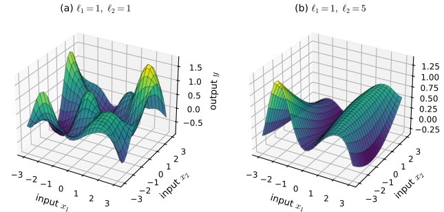
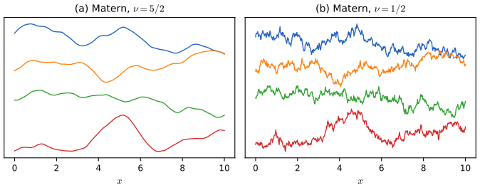
pp. 569–571 A kernel is stationary if it depends on the inputs only through \(\bm r=\bm x-\bm x'\) (and isotropic if only through \(\|\bm r\|\)). ARD. Replacing the Euclidean distance in the SE kernel by a Mahalanobis distance gives \(\kern(\bm r)=\sigma^2\exp(-\frac12\bm r^\T\bm\Sigma^{-1}\bm r)\) (17.7); with \(\bm\Sigma=\diag(\ell_1^2,\dots,\ell_D^2)\) it factorises into one-dimensional SE kernels, \[ \kern(\bm r;\bm\ell,\sigma^2)=\sigma^2\exp\Big(-\frac12\sum_{d=1}^D\frac{r_d^2}{\ell_d^2}\Big)=\prod_{d=1}^D\kern(r_d;\ell_d,\sigma^{2/D}),\qquad\kern(r;\ell,\tau^2)=\tau^2\exp\Big(-\frac{r^2}{2\ell^2}\Big), \tag{17.8, 17.9} \] (the amplitudes multiply to \((\sigma^{2/D})^D=\sigma^2\)). A large \(\ell_d\) switches input \(d\) off: automatic relevance determination (Figure 17.1). Matern. \[ \kern(r;\nu,\ell)=\frac{2^{1-\nu}}{\Gamma(\nu)}\Big(\frac{\sqrt{2\nu}\,r}{\ell}\Big)^\nu K_\nu\Big(\frac{\sqrt{2\nu}\,r}{\ell}\Big), \tag{17.10} \] with \(K_\nu\) the modified Bessel function of the second kind. Sample paths are rougher than under the SE kernel (Figure 17.2): the process is \(k\) times differentiable (in mean square) iff \(\nu>k\), and the kernel tends to the SE kernel as \(\nu\to\infty\). For half-integer \(\nu\) the Bessel function is elementary: \[ \kern(r;\tfrac12,\ell)=e^{-r/\ell},\quad \kern(r;\tfrac32,\ell)=\Big(1+\frac{\sqrt3r}{\ell}\Big)e^{-\sqrt3r/\ell},\quad \kern(r;\tfrac52,\ell)=\Big(1+\frac{\sqrt5r}{\ell}+\frac{5r^2}{3\ell^2}\Big)e^{-\sqrt5r/\ell}. \tag{17.11–17.13} \] \(\nu=\frac12\) is the Ornstein-Uhlenbeck process, continuous but nowhere differentiable.
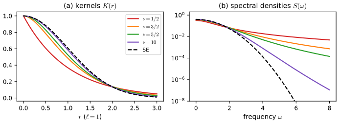
Filling the gap 17.3: Bochner's theorem, the Matern spectral density, the closed forms (17.11)–(17.13), the limit \(\nu\to\infty\) and "differentiable iff \(\nu>k\)" pp. 569–571, (17.7)–(17.13)
Derivation
Bochner's theorem. A continuous stationary \(\kern(\bm r)\) on \(\R^D\) is PSD iff \(\kern(\bm r)=\int e^{i\bm\omega^\T\bm r}\,\d\mu(\bm\omega)\) for a finite nonnegative symmetric measure \(\mu\) (the spectral measure; its density, when it exists, is the spectral density \(S\)). The direction used in this chapter is the easy one: if \(\kern\) has this form then, exactly as in Result 17.1, \[ \sum_{ij}c_ic_j\kern(\bm x_i-\bm x_j)=\int|\sum_jc_je^{i\bm\omega^\T\bm x_j}|^2\d\mu\ge0 \]. The converse (every continuous stationary PSD kernel has such a representation) is Bochner (1933); it is what makes the spectral density a complete description of a stationary kernel. Examples: the SE kernel has \(S(\bm\omega)=\N(\bm\omega\given\bm 0,\ell^{-2}\bm I)\) (the Fourier transform of a Gaussian), and this is the basis of the random features of Section 17.2.9.3.
The Matern spectral density. In one dimension, with \(a=\sqrt{2\nu}/\ell\), \[ S_\nu(\omega)=\frac{\Gamma(\nu+\frac12)}{\Gamma(\nu)\sqrt\pi}\,\frac{a^{2\nu}}{(a^2+\omega^2)^{\nu+1/2}} . \] Basset's integral for \(K_\nu\) (Watson, 1944), \[ \int_0^\infty\cos(\omega r)(a^2+\omega^2)^{-\nu-1/2}\,\d\omega=\frac{\sqrt\pi}{\Gamma(\nu+\frac12)}\big(\frac r{2a}\big)^\nu K_\nu(ar) \], gives \[ \int_{-\infty}^\infty S_\nu(\omega)\cos(\omega r)\,\d\omega=\frac{2a^{2\nu}}{\Gamma(\nu)}\Big(\frac r{2a}\Big)^\nu K_\nu(ar)=\frac{2^{1-\nu}}{\Gamma(\nu)}(ar)^\nu K_\nu(ar), \] which is (17.10). So the Matern kernel is PSD by Bochner's theorem, and strictly PD because \(S_\nu>0\) everywhere. (In \(D\) dimensions the exponent is \(\nu+D/2\).) The identity was confirmed numerically for \(\nu=\frac12,\frac32,4\) (quadrature against (17.10), agreement to \(10^{-7}\)).
Closed forms. For half-integer order, \(K_{1/2}(z)=\sqrt{\pi/(2z)}\,e^{-z}\), \(K_{3/2}(z)=\sqrt{\pi/(2z)}\,e^{-z}(1+z^{-1})\), \(K_{5/2}(z)=\sqrt{\pi/(2z)}\,e^{-z}(1+3z^{-1}+3z^{-2})\). With \(z=\sqrt{2\nu}\,r/\ell\): \(\nu=\frac12\): \(\frac{2^{1/2}}{\sqrt\pi}z^{1/2}\sqrt{\frac\pi{2z}}e^{-z}=e^{-z}\), \(z=r/\ell\), which is (17.11); \(\nu=\frac32\): \(\frac{2^{-1/2}}{\sqrt\pi/2}z^{3/2}\sqrt{\frac\pi{2z}}e^{-z}(1+z^{-1})=(1+z)e^{-z}\), \(z=\sqrt3r/\ell\), which is (17.12); \(\nu=\frac52\): \[ \frac{2^{-3/2}}{3\sqrt\pi/4}z^{5/2}\sqrt{\frac\pi{2z}}e^{-z}(1+3z^{-1}+3z^{-2})=(1+z+\frac{z^2}3)e^{-z} \], \(z=\sqrt5r/\ell\), and \(z^2/3=5r^2/(3\ell^2)\) gives (17.13).
The limit \(\nu\to\infty\). Write \(S_\nu(\omega)=c_\nu\,(1+\ell^2\omega^2/(2\nu))^{-\nu-1/2}\) with \(c_\nu=\frac{\Gamma(\nu+1/2)}{\Gamma(\nu)\sqrt\pi}\frac{\ell}{\sqrt{2\nu}}\). Since \(\Gamma(\nu+\frac12)/\Gamma(\nu)\sim\sqrt\nu\), \(c_\nu\to\ell/\sqrt{2\pi}\); and \((1+u/\nu)^{-\nu-1/2}\to e^{-u}\) with \(u=\ell^2\omega^2/2\). So \(S_\nu\) converges pointwise to \(\frac{\ell}{\sqrt{2\pi}}e^{-\ell^2\omega^2/2}\), the spectral density of the SE kernel. For \(\nu\ge2\), the binomial inequality \((1+u/\nu)^\nu\ge1+u+\frac{\nu-1}{2\nu}u^2\ge1+u+u^2/4\) gives the integrable bound \(S_\nu(\omega)\le C/(1+u+u^2/4)\), so by dominated convergence \(\int S_\nu\cos(\omega r)\,\d\omega\to e^{-r^2/(2\ell^2)}\) for every \(r\). Numerically the maximum gap to the SE kernel is \(8.4\times10^{-2}\), \(2.3\times10^{-2}\), \(7.7\times10^{-3}\) and \(2.3\times10^{-3}\) at \(\nu=2.5,10,30,100\) (Figure 17.S2).
Differentiability. Let \(f\) be a zero-mean stationary process on \(\R\) with covariance \(\kern(r)=\int e^{i\omega r}\d\mu\). Then \[ \E[(\sum_ja_jf(x_j))(\sum_kb_kf(x_k))]=\int(\sum_ja_je^{i\omega x_j})\overline{(\sum_kb_ke^{i\omega x_k})}\,\d\mu \]. The difference quotient \(D_h=(f(x+h)-f(x))/h\) therefore has \(\E[(D_h-D_{h'})^2]=\int|\frac{e^{i\omega h}-1}h-\frac{e^{i\omega h'}-1}{h'}|^2\d\mu\). If \(\int\omega^2\d\mu<\infty\), the integrand is bounded by \(4\omega^2\) and tends to 0, so \(D_h\) is Cauchy in \(L^2\): \(f\) is mean-square differentiable. If instead \(f\) is m.s. differentiable, \(\E D_h^2=\int\frac{2(1-\cos\omega h)}{h^2}\d\mu\) stays bounded, and Fatou's lemma gives \(\int\omega^2\d\mu\le\liminf\E D_h^2<\infty\). Iterating, \(f\) is \(k\) times m.s. differentiable iff \(\int\omega^{2k}\d\mu<\infty\). For the Matern kernel \(S_\nu(\omega)\asymp|\omega|^{-2\nu-1}\), and \(\int^\infty\omega^{2k-2\nu-1}\d\omega<\infty\iff k<\nu\). So "\(k\) times differentiable iff \(\nu>k\)" holds in mean square; sample paths have the same smoothness up to the boundary case (Stein, 1999, Section 2.7). The SE spectral density has all moments, hence infinitely differentiable paths. (Numerically, \(\int_0^W\omega^2S_\nu\) grows tenfold from \(W=10^2\) to \(10^3\) for \(\nu=\frac12\) and is unchanged to \(2\times10^{-5}\) for \(\nu=\frac52\).) \(\square\)
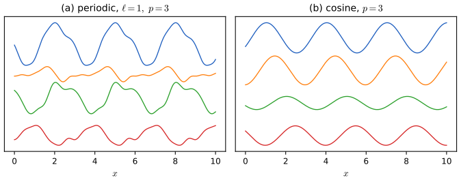
p. 571 Periodic kernels. \(\kern_{\rm per}(r;\ell,p)=\exp(-\frac2{\ell^2}\sin^2(\pi r/p))\) (17.14) gives functions that repeat with period \(p\); the cosine kernel \(\kern(r;p)=\cos(2\pi r/p)\) (17.15) gives pure sinusoids (Figure 17.3).
Filling the gap 17.4: why the periodic and cosine kernels are valid, and why cosine samples are sinusoids p. 571, (17.14)–(17.15)
Derivation
Map \(x\in\R\) to the circle, \(\bm u(x)=(\cos(2\pi x/p),\sin(2\pi x/p))\). Then \(\|\bm u(x)-\bm u(x')\|^2=2-2\cos(2\pi r/p)=4\sin^2(\pi r/p)\), so \[ \kern_{\rm per}(x,x')=\exp\Big(-\frac{\|\bm u(x)-\bm u(x')\|^2}{2\ell^2}\Big), \] the SE kernel applied to \(\bm u(x)\) and \(\bm u(x')\). A kernel composed with any map is a kernel (its Gram matrix on \(\{x_i\}\) is the Gram matrix of the original kernel on \(\{\bm u(x_i)\}\)), so (17.14) is valid; the identity is confirmed numerically to \(10^{-13}\). Likewise \(\cos(2\pi(x-x')/p)=\bm u(x)^\T\bm u(x')\) is the linear kernel on \(\bm u\): valid, with Gram matrices of rank at most 2. A zero-mean GP with this kernel is \(f(x)=a\cos(2\pi x/p)+b\sin(2\pi x/p)\) with \(a,b\) independent \(\N(0,1)\) (its covariance is exactly \(\bm u(x)^\T\bm u(x')\)), i.e. a sinusoid of period \(p\) with random amplitude \(\sqrt{a^2+b^2}\) and uniform random phase, which is what Figure 17.3b shows. \(\square\)
See also: Bayesian and Probabilistic ML, gap 6.9 (sampling a GP; the exponential kernel is the Ornstein-Uhlenbeck process) and gap 6.12 (valid and invalid kernels on the circle); the kernel functions demo.
17.1.2.2 Making new kernels from old
p. 572 If \(\kern_1,\kern_2\) are valid, so are \(c\kern_1\) for \(c>0\) (17.16), \(f(\bm x)\kern_1(\bm x,\bm x')f(\bm x')\) for any \(f\) (17.17), \(q(\kern_1)\) for any polynomial \(q\) with nonnegative coefficients (17.18), \(\exp(\kern_1)\) (17.19), and \(\bm x^\T\bm A\bm x'\) for any PSD \(\bm A\) (17.20). From the linear kernel these give the polynomial kernels \((\bm x^\T\bm x')^M\) (all monomials of degree \(M\)) and \((\bm x^\T\bm x'+c)^M\) (all monomials up to degree \(M\)) (17.21, 17.22), and, since \(\|\bm x-\bm x'\|^2=\bm x^\T\bm x+\bm x'^\T\bm x'-2\bm x^\T\bm x'\) (17.23), the Gaussian kernel \[ \exp\Big(-\frac{\|\bm x-\bm x'\|^2}{2\sigma^2}\Big)=e^{-\bm x^\T\bm x/(2\sigma^2)}\,e^{\bm x^\T\bm x'/\sigma^2}\,e^{-\bm x'^\T\bm x'/(2\sigma^2)} \tag{17.24} \] is valid: the middle factor is \(\exp\) of a positive multiple of the linear kernel, (17.16) and (17.19), and the outer factors are \(f(\bm x)f(\bm x')\), (17.17).
17.1.2.3 Combining kernels by addition and multiplication
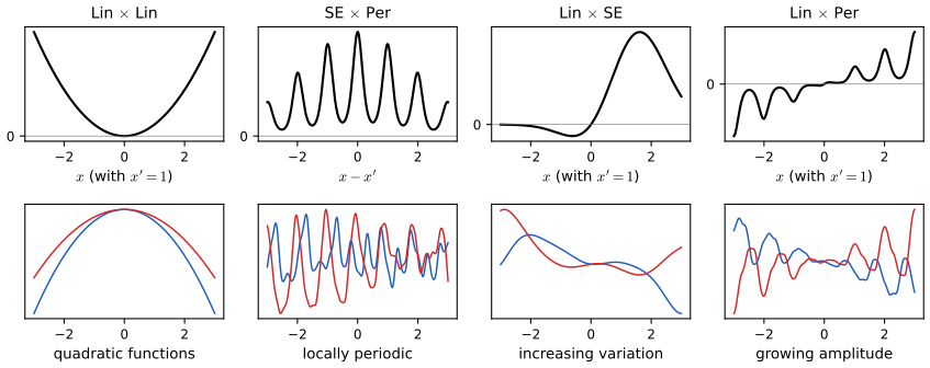
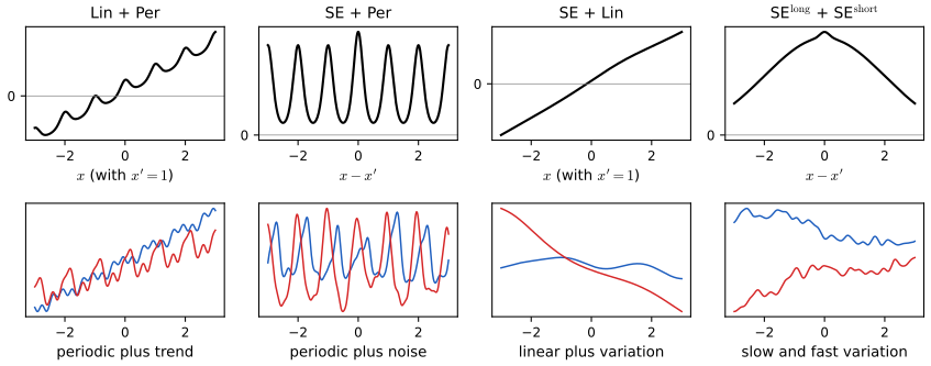
pp. 572–573 Sums \(\kern_1+\kern_2\) (17.25) and products \(\kern_1\kern_2\) (17.26) of kernels are kernels. A sum behaves like a disjunction of the two structures (a trend plus a periodic part, slow plus fast variation, Figure 17.5); a product like a conjunction (similar only if similar under both: locally periodic functions, growing amplitude, Figure 17.4).
Filling the gap 17.5: Result 17.3 (the closure rules (17.16)–(17.20), (17.25), (17.26)) and what sums and products mean pp. 572–573
Derivation
Fix distinct points and write \(\bm K_1,\bm K_2\) for the Gram matrices; it suffices to show each new Gram matrix is PSD.
(17.16) \(\bm c^\T(c\bm K_1)\bm c=c\,\bm c^\T\bm K_1\bm c\ge0\). (17.25) \(\bm c^\T(\bm K_1+\bm K_2)\bm c\) is a sum of two nonnegative numbers. (17.17) The Gram matrix is \(\bm F\bm K_1\bm F\) with \(\bm F=\diag(f(\bm x_i))\), and \(\bm c^\T\bm F\bm K_1\bm F\bm c=(\bm F\bm c)^\T\bm K_1(\bm F\bm c)\ge0\). (17.20) \(\bm c^\T\bm X\bm A\bm X^\T\bm c=(\bm X^\T\bm c)^\T\bm A(\bm X^\T\bm c)\ge0\).
(17.26) Schur product theorem. Write \(\bm K_1=\sum_m\lambda_m\bm v_m\bm v_m^\T\) with \(\lambda_m\ge0\). The Gram matrix of the product kernel is the entrywise (Hadamard) product \[ \bm K_1\circ\bm K_2=\sum_m\lambda_m(\bm v_m\bm v_m^\T)\circ\bm K_2=\sum_m\lambda_m\diag(\bm v_m)\bm K_2\diag(\bm v_m) \], a nonnegative combination of matrices that are PSD by the argument for (17.17).
(17.18) \(q(\kern_1)=\sum_ka_k\kern_1^k\) with \(a_k\ge0\): the constant term \(a_0\bm 1\bm 1^\T\) is PSD, \(\kern_1^k\) is a kernel by \(k-1\) applications of the Schur product theorem, and the sum is PSD by (17.16) and (17.25). (17.19) The partial sums \(\sum_{k\le n}\bm K_1^{\circ k}/k!\) are PSD by (17.18) and converge entrywise to the Gram matrix of \(\exp(\kern_1)\); the set of PSD matrices is closed (it is an intersection of the closed half-spaces \(\{\bm A:\bm c^\T\bm A\bm c\ge0\}\)), so the limit is PSD.
Typos in (17.21)–(17.22). The expansions should read \((x_1x_1'+x_2x_2')^2=(x_1x_1')^2+(x_2x_2')^2+2(x_1x_1')(x_2x_2')\) and contain \((x_2x_2')(x_1x_1')\); the book drops two primes. The text also calls \(\bm X\bm X^\T\) "the (scaled) covariance matrix of the data"; it is the \(N\times N\) matrix of inner products (the covariance is the \(D\times D\) matrix \(\frac1N\bm X^\T\bm X\) of centred data), PSD because \(\bm c^\T\bm X\bm X^\T\bm c=\|\bm X^\T\bm c\|^2\).
Sums and products as structure. If \(f_1\sim\GP(0,\kern_1)\) and \(f_2\sim\GP(0,\kern_2)\) are independent, \(f_1+f_2\) is a GP with kernel \(\kern_1+\kern_2\): the function has both structures at once, and either can explain a feature of the data. The product \(f_1f_2\) has covariance \(\E[f_1(x)f_2(x)f_1(x')f_2(x')]=\kern_1(x,x')\kern_2(x,x')\) (it is not Gaussian, but a GP with kernel \(\kern_1\kern_2\) has the same covariance): two inputs are strongly correlated only if both kernels say so. With \(\kern_1=\) SE and \(\kern_2=\) periodic this gives patterns that repeat but slowly change shape ("locally periodic"); with a linear kernel \(xx'\) as one factor, the variance \(x^2\kern_2(x,x)\) grows with \(|x|\) ("growing amplitude"). All seven rules were confirmed on random Gram matrices (smallest eigenvalues at rounding level). Proofs in the companion course: Bayesian and Probabilistic ML, Result 6.3. \(\square\)
17.1.2.4 Kernels for structured inputs
p. 573 Kernels need no vector representation of the inputs, only a PSD similarity, so they apply to strings (e.g. counting shared \(n\)-grams: the inner product of \(n\)-gram count vectors, hence valid) and graphs (e.g. the random walk kernel, which counts common walks in the two graphs and can be computed through the product graph). Validity of such kernels follows from writing them as inner products of (possibly huge) count vectors, exactly as in (17.5).
17.2 Gaussian processes
p. 574 A Gaussian process \(f\sim\GP(m,\kern)\) is a random function such that for every finite set of inputs \(\bm x_1,\dots,\bm x_M\) the vector \((f(\bm x_1),\dots,f(\bm x_M))\) is Gaussian with mean \((m(\bm x_i))_i\) and covariance \([\kern(\bm x_i,\bm x_j)]_{ij}\). The kernel must be PSD for these to be covariance matrices, and the family of finite-dimensional laws is consistent (marginalising a Gaussian drops rows and columns), so by Kolmogorov's extension theorem such a process exists. Prediction is then Gaussian conditioning on the \(N+1\) (or \(N+N_*\)) dimensional vector of training and test function values (Figure 17.6, a diagram, is not reproduced).
17.2.1 Noise-free observations
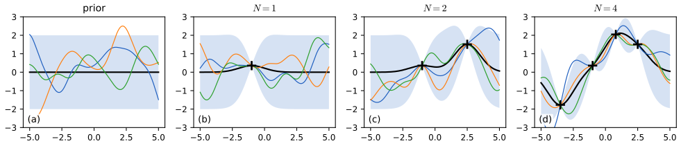
pp. 574–575 If \(y_n=f(\bm x_n)\) exactly, the joint law of training values \(\bm f_X\) and test values \(\bm f_*\) is \[ \begin{pmatrix}\bm f_X\\\bm f_*\end{pmatrix}\sim\N\left(\begin{pmatrix}\bm\mu_X\\\bm\mu_*\end{pmatrix},\begin{pmatrix}\bm K_{X,X}&\bm K_{X,*}\\\bm K_{X,*}^\T&\bm K_{*,*}\end{pmatrix}\right), \tag{17.27} \] and conditioning gives \(p(\bm f_*\given\bm X_*,\mathcal D)=\N(\bm f_*\given\bm\mu_{*|X},\bm\Sigma_{*|X})\) with \[ \bm\mu_{*|X}=m(\bm X_*)+\bm K_{X,*}^\T\bm K_{X,X}^{-1}(\bm f_X-m(\bm X)),\qquad \bm\Sigma_{*|X}=\bm K_{*,*}-\bm K_{X,*}^\T\bm K_{X,X}^{-1}\bm K_{X,*}. \tag{17.28–17.30} \] The posterior interpolates the data and its uncertainty grows away from them (Figure 17.7).
17.2.2 Noisy observations
pp. 575–576 With \(y_n=f(\bm x_n)+\epsilon_n\), \(\epsilon_n\sim\N(0,\sigma_y^2)\) independent of \(f\), \(\cov[y_i,y_j]=\kern(\bm x_i,\bm x_j)+\sigma_y^2\delta_{ij}\), i.e. \(\cov[\bm y\given\bm X]=\bm K_{X,X}+\sigma_y^2\bm I_N=\bm K_\sigma\) (17.31, 17.32), and \(\cov[\bm y,\bm f_*]=\bm K_{X,*}\). Conditioning on \(\bm y\) in the joint law (17.33): \[ \bm\mu_{*|X}=\bm\mu_*+\bm K_{X,*}^\T\bm K_\sigma^{-1}(\bm y-\bm\mu_X),\qquad\bm\Sigma_{*|X}=\bm K_{*,*}-\bm K_{X,*}^\T\bm K_\sigma^{-1}\bm K_{X,*}; \tag{17.34–17.36} \] for one test point and zero mean, \[ p(f_*\given\mathcal D,\bm x_*)=\N\big(f_*\given\bm k_*^\T\bm K_\sigma^{-1}\bm y,\;k_{**}-\bm k_*^\T\bm K_\sigma^{-1}\bm k_*\big),\qquad \mu_{*|X}=\bm k_*^\T\bm\alpha=\sum_{n=1}^N\kern(\bm x_*,\bm x_n)\alpha_n,\ \ \bm\alpha=\bm K_\sigma^{-1}\bm y . \tag{17.37, 17.38} \] The mean is a linear combination of \(N\) kernel functions centred at the data, the same form as kernel ridge regression (17.108). The predictive law of a new noisy observation \(y_*\) adds \(\sigma_y^2\) to the variance.
Filling the gap 17.6: the conditioning formulas (17.28)–(17.38), and why the noise-free GP interpolates pp. 574–576
Derivation
Gaussian conditioning in three lines. Let \((\bm a,\bm b)\) be jointly Gaussian with means \(\bm\mu_a,\bm\mu_b\), covariances \(\bm\Sigma_{aa},\bm\Sigma_{bb}\), cross-covariance \(\bm\Sigma_{ab}\), and \(\bm\Sigma_{aa}\) invertible. Put \(\bm z=\bm b-\bm\Sigma_{ab}^\T\bm\Sigma_{aa}^{-1}\bm a\). Then \[ \cov[\bm z,\bm a]=\bm\Sigma_{ab}^\T-\bm\Sigma_{ab}^\T\bm\Sigma_{aa}^{-1}\bm\Sigma_{aa}=\bm 0 \], and since \((\bm z,\bm a)\) is jointly Gaussian, \(\bm z\) is independent of \(\bm a\). Hence, given \(\bm a\), \(\bm b=\bm z+\bm\Sigma_{ab}^\T\bm\Sigma_{aa}^{-1}\bm a\) is Gaussian with mean \[ \E\bm z+\bm\Sigma_{ab}^\T\bm\Sigma_{aa}^{-1}\bm a=\bm\mu_b+\bm\Sigma_{ab}^\T\bm\Sigma_{aa}^{-1}(\bm a-\bm\mu_a) \] and covariance \(\cov\bm z=\bm\Sigma_{bb}-\bm\Sigma_{ab}^\T\bm\Sigma_{aa}^{-1}\bm\Sigma_{ab}\). With \(\bm a=\bm f_X\), \(\bm b=\bm f_*\) this is (17.29)–(17.30); with \(\bm a=\bm y\), whose covariance is \(\bm K_\sigma\) and whose cross-covariance with \(\bm f_*\) is \(\cov[\bm f_X+\bm\epsilon,\bm f_*]=\bm K_{X,*}\) (the noise is independent of \(f\)), it is (17.35)–(17.36). (The general result, with the information form, is proved in Section 3.2.3 of these notes.)
Interpolation. Take a test point equal to a training input, \(\bm x_*=\bm x_n\). Then \(\bm k_*\) is the \(n\)-th column of \(\bm K_{X,X}\), i.e. \(\bm k_*=\bm K_{X,X}\bm e_n\), so in the noise-free case \(\mu_*=\bm e_n^\T\bm K_{X,X}\bm K_{X,X}^{-1}\bm f_X=f_n\) and \(\sigma_*^2=k_{nn}-\bm e_n^\T\bm K_{X,X}\bm e_n=0\): the GP returns the observed value with no uncertainty. With noise, \(\mu_*=\bm e_n^\T\bm K_{X,X}(\bm K_{X,X}+\sigma_y^2\bm I)^{-1}\bm y\), a shrunken value (gap 17.7). In the code the noise-free posterior is computed with a jitter \(10^{-10}\); its variance at the data is below \(10^{-9}\) and its mean equals the data to \(10^{-6}\). See also Bayesian and Probabilistic ML, Result 6.4. \(\square\)
17.2.3 Comparison to kernel regression
pp. 576–577 Kernel (Nadaraya-Watson) regression predicts \(\E[y\given\bm x,\mathcal D]=\sum_ny_nw_n(\bm x)\) with \(w_n(\bm x)=\kern_h(\bm x-\bm x_n)/\sum_{n'}\kern_h(\bm x-\bm x_{n'})\) (17.39, 17.40), also a weighted sum of the responses. The differences: a GP uses a Mercer kernel (so structured inputs are allowed), interpolates when \(\sigma_y=0\), learns its kernel by maximising the marginal likelihood instead of by cross-validation, and costs \(O(N^3)\) to fit against \(O(N)\) per prediction for kernel regression.
Filling the gap 17.7: the GP as a linear smoother, its equivalent kernel, and why kernel regression does not interpolate pp. 576–577, (17.38)–(17.40)
Derivation
The GP mean is a weighted sum of the responses too. \(\mu_*=\bm k_*^\T\bm K_\sigma^{-1}\bm y=\sum_nh_n(\bm x_*)y_n\) with weights \(\bm h(\bm x_*)=\bm K_\sigma^{-1}\bm k_*\), the equivalent kernel. Unlike the Nadaraya-Watson weights, which are positive and sum to one, these can be negative and need not sum to one: they come from solving a linear system, not from normalising a similarity. At the training inputs the fitted values are \(\bm S\bm y\) with the smoother matrix \(\bm S=\bm K(\bm K+\sigma_y^2\bm I)^{-1}\). If \(\bm K=\bm U\bm\Lambda\bm U^\T\), then \(\bm S=\bm U\diag(\lambda_i/(\lambda_i+\sigma_y^2))\bm U^\T\): each eigen-direction of the data is shrunk by a factor in \([0,1)\), strongly for the small eigenvalues (rough directions) and weakly for the large ones; \(\tr\bm S\) is the effective number of parameters. When \(\sigma_y^2\to0\) and \(\bm K\) is invertible, \(\bm S\to\bm I\): interpolation.
Kernel regression does not interpolate. Its fitted value at \(\bm x_n\) is \(\sum_mw_m(\bm x_n)y_m\) with \(w_n(\bm x_n)=\kern_h(\bm 0)/\sum_m\kern_h(\bm x_n-\bm x_m)<1\) as soon as any other point has positive kernel weight, so the fit is a proper average of \(y_n\) and its neighbours and differs from \(y_n\) unless the neighbours share its value. On the 7 points of Figure 17.9 with an SE kernel of width 1, the Nadaraya-Watson fit misses the data by up to 0.53, while the noise-free GP reproduces them. (It can be turned into an interpolator by repeatedly smoothing the residuals, as the book notes.) See also Elements of Statistical Learning, 6.1 and Bayesian and Probabilistic ML, 6.3.1. \(\square\)
17.2.4 Weight space vs function space
p. 577 Bayesian linear regression \(f(\bm x)=\bm w^\T\phi(\bm x)\) with prior \(\bm w\sim\N(\bm 0,\bm\Sigma_w)\) has posterior \(\N(\bm w\given\sigma_y^{-2}\bm A^{-1}\bm\Phi^\T\bm y,\bm A^{-1})\), \(\bm A=\sigma_y^{-2}\bm\Phi^\T\bm\Phi+\bm\Sigma_w^{-1}\) (17.41, 17.42), and predictive \[ p(f_*\given\mathcal D,\bm x_*)=\N\big(f_*\given\sigma_y^{-2}\phi_*^\T\bm A^{-1}\bm\Phi^\T\bm y,\;\phi_*^\T\bm A^{-1}\phi_*\big). \tag{17.43} \] This is exactly the GP prediction (17.37) with kernel \(\kern(\bm x,\bm x')=\phi(\bm x)^\T\bm\Sigma_w\phi(\bm x')\): \[ \mu_{*|X}=\phi_*^\T\bm\Sigma_w\bm\Phi^\T(\bm K+\sigma_y^2\bm I)^{-1}\bm y=\bm k_*^\T\bm K_\sigma^{-1}\bm y,\qquad \Sigma_{*|X}=k_{**}-\bm k_*^\T\bm K_\sigma^{-1}\bm k_*. \tag{17.44–17.46} \] The "weight-space" computation inverts a \(D\times D\) matrix, the "function-space" one an \(N\times N\) matrix, and the latter only needs the kernel, which may correspond to infinitely many features.
Filling the gap 17.8: from (17.43) to (17.45)–(17.46) with the matrix inversion lemma p. 577
Derivation
Let \(\bm K=\bm\Phi\bm\Sigma_w\bm\Phi^\T\), \(\bm k_*=\bm\Phi\bm\Sigma_w\phi_*\), \(k_{**}=\phi_*^\T\bm\Sigma_w\phi_*\). Push-through identity. \[ \bm\Phi^\T(\bm K+\sigma_y^2\bm I)=\bm\Phi^\T\bm\Phi\bm\Sigma_w\bm\Phi^\T+\sigma_y^2\bm\Phi^\T=\sigma_y^2(\sigma_y^{-2}\bm\Phi^\T\bm\Phi+\bm\Sigma_w^{-1})\bm\Sigma_w\bm\Phi^\T=\sigma_y^2\bm A\bm\Sigma_w\bm\Phi^\T . \] Multiplying by \(\bm A^{-1}\) on the left and \((\bm K+\sigma_y^2\bm I)^{-1}\) on the right: \(\bm A^{-1}\bm\Phi^\T=\sigma_y^2\bm\Sigma_w\bm\Phi^\T(\bm K+\sigma_y^2\bm I)^{-1}\). So the mean in (17.43) is \[ \sigma_y^{-2}\phi_*^\T\bm A^{-1}\bm\Phi^\T\bm y=\phi_*^\T\bm\Sigma_w\bm\Phi^\T\bm K_\sigma^{-1}\bm y=\bm k_*^\T\bm K_\sigma^{-1}\bm y \], which is (17.45).
Woodbury identity. \[ (\bm\Sigma_w^{-1}+\bm\Phi^\T\sigma_y^{-2}\bm\Phi)^{-1}=\bm\Sigma_w-\bm\Sigma_w\bm\Phi^\T(\sigma_y^2\bm I+\bm\Phi\bm\Sigma_w\bm\Phi^\T)^{-1}\bm\Phi\bm\Sigma_w \] (check: multiply the right side by \(\bm A\) and simplify with the push-through identity; see Section 7.3.3). Hence \(\phi_*^\T\bm A^{-1}\phi_*=k_{**}-\bm k_*^\T\bm K_\sigma^{-1}\bm k_*\), which is (17.46). Both identities hold for any PD \(\bm\Sigma_w\) and any \(\bm\Phi\); a random instance agrees to \(10^{-9}\). If \(D<N\), \(\bm K\) has rank at most \(D\): a finite-feature GP is a degenerate GP, and its posterior variance far from the data is bounded by what \(D\) features allow. A nonzero mean is absorbed by a constant feature. Companion proof: Bayesian and Probabilistic ML, gap 6.10. \(\square\)
17.2.5 Numerical issues
pp. 577–578 Never invert \(\bm K_\sigma\). Factor \(\bm K_\sigma=\bm L\bm L^\T\) (Cholesky, \(O(N^3)\)), solve \(\bm\alpha=\bm L^\T\backslash(\bm L\backslash\bm y)\), and then for each test point \[ \mu_*=\bm k_*^\T\bm\alpha,\qquad\sigma_*^2=k_{**}-\bm v^\T\bm v,\ \bm v=\bm L\backslash\bm k_*,\qquad \log p(\bm y\given\bm X)=-\tfrac12\bm y^\T\bm\alpha-\sum_{n=1}^N\log L_{nn}-\tfrac N2\log(2\pi), \tag{17.47–17.49} \] at cost \(O(N)\) for the mean and \(O(N^2)\) for the variance.
17.2.6 Estimating the kernel
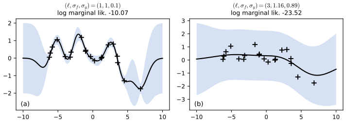
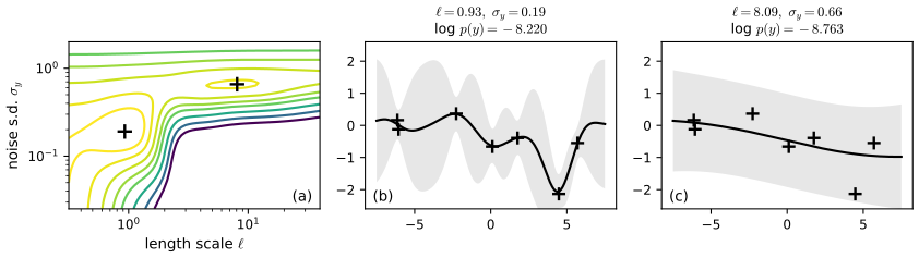
pp. 578–580 Kernel parameters have a large effect on the fit. For the SE kernel \(\kern(x_p,x_q)=\sigma_f^2\exp(-\frac1{2\ell^2}(x_p-x_q)^2)\) (17.50) with noise \(\sigma_y\), \(\ell\) sets the horizontal scale of variation and \(\sigma_f\) the vertical one (Figure 17.8).
17.2.6.1 Empirical Bayes
pp. 579–580 Choose \(\bm\theta\) by maximising the marginal likelihood (type-II maximum likelihood, Section 4.6.5.3) \[ p(\bm y\given\bm X,\bm\theta)=\int p(\bm y\given\bm f,\bm X)p(\bm f\given\bm X,\bm\theta)\,\d\bm f,\qquad \log p(\bm y\given\bm X,\bm\theta)=-\tfrac12\bm y^\T\bm K_\sigma^{-1}\bm y-\tfrac12\log|\bm K_\sigma|-\tfrac N2\log(2\pi), \tag{17.51, 17.52} \] a data-fit term, a complexity penalty and a constant. Its gradient is \[ \frac{\partial}{\partial\theta_j}\log p(\bm y\given\bm X,\bm\theta)=\tfrac12\bm y^\T\bm K_\sigma^{-1}\frac{\partial\bm K_\sigma}{\partial\theta_j}\bm K_\sigma^{-1}\bm y-\tfrac12\tr\Big(\bm K_\sigma^{-1}\frac{\partial\bm K_\sigma}{\partial\theta_j}\Big)=\tfrac12\tr\Big((\bm\alpha\bm\alpha^\T-\bm K_\sigma^{-1})\frac{\partial\bm K_\sigma}{\partial\theta_j}\Big), \tag{17.53, 17.54} \] \(O(N^3)\) once and \(O(N^2)\) per parameter. The surface is not concave and can have several local maxima (Figure 17.9).
Filling the gap 17.9: the Cholesky formulas, the marginal likelihood, its gradient, and the shape of the surface in Figure 17.9 pp. 577–580, (17.47)–(17.54)
Derivation
Cholesky formulas. From \(\bm K_\sigma=\bm L\bm L^\T\), \(\bm K_\sigma^{-1}=\bm L^{-\T}\bm L^{-1}\), so \(\bm\alpha=\bm L^{-\T}(\bm L^{-1}\bm y)\) (two triangular solves, \(O(N^2)\)) and \(\bm k_*^\T\bm K_\sigma^{-1}\bm k_*=\|\bm L^{-1}\bm k_*\|^2=\bm v^\T\bm v\), giving (17.47)–(17.48). Since \(|\bm K_\sigma|=|\bm L|^2=\prod_nL_{nn}^2\), \(\frac12\log|\bm K_\sigma|=\sum_n\log L_{nn}\), giving (17.49). The Cholesky factorisation is backward stable and costs \(N^3/3\) flops, a third of an explicit inverse; if \(\bm K_\sigma\) is numerically singular (tiny \(\sigma_y\), long \(\ell\)), a jitter \(\epsilon\bm I\) is added.
The marginal likelihood (17.52). \(\bm y=\bm f_X+\bm\epsilon\) with \(\bm f_X\sim\N(\bm 0,\bm K)\) and \(\bm\epsilon\sim\N(\bm 0,\sigma_y^2\bm I)\) independent, so \(\bm y\sim\N(\bm 0,\bm K+\sigma_y^2\bm I)\) and the integral (17.51) needs no computation: (17.52) is the log density of this Gaussian. It agrees with a library implementation of GP regression to 10 digits.
The gradient (17.53)–(17.54). Two matrix facts. (i) Differentiating \(\bm K\bm K^{-1}=\bm I\) gives \(\partial(\bm K^{-1})=-\bm K^{-1}(\partial\bm K)\bm K^{-1}\). (ii) \(\partial\log|\bm K|=\tr(\bm K^{-1}\partial\bm K)\): \[ |\bm K+t\bm B|=|\bm K|\,|\bm I+t\bm K^{-1}\bm B|=|\bm K|(1+t\tr(\bm K^{-1}\bm B)+O(t^2)) \]. Then \[ \partial_j(-\frac12\bm y^\T\bm K_\sigma^{-1}\bm y)=\frac12\bm y^\T\bm K_\sigma^{-1}(\partial_j\bm K_\sigma)\bm K_\sigma^{-1}\bm y=\frac12\bm\alpha^\T(\partial_j\bm K_\sigma)\bm\alpha=\frac12\tr(\bm\alpha\bm\alpha^\T\partial_j\bm K_\sigma) \], and \[ \partial_j(-\frac12\log|\bm K_\sigma|)=-\frac12\tr(\bm K_\sigma^{-1}\partial_j\bm K_\sigma) \]. Adding gives (17.54). For symmetric matrices \(\tr(\bm A\bm B)=\sum_{ij}A_{ij}B_{ij}\), so each parameter costs \(O(N^2)\) once \(\bm K_\sigma^{-1}\) is known. For the SE kernel in log parameters (positivity for free): \(\partial\bm K_\sigma/\partial\log\ell=\bm K_f\circ\bm D^{(2)}/\ell^2\) with \(D^{(2)}_{pq}=(x_p-x_q)^2\), \(\partial\bm K_\sigma/\partial\log\sigma_f=2\bm K_f\), \(\partial\bm K_\sigma/\partial\log\sigma_y=2\sigma_y^2\bm I\). These agree with finite differences to \(10^{-6}\). (Same result in the companion course: Bayesian and Probabilistic ML, gap 6.13.)
Why the surface looks as it does. Fix \(\sigma_f=1\). (a) Very short length scale. For distinct inputs, \(\bm K_f\to\sigma_f^2\bm I\) as \(\ell\to0\), so \(\log p\to\log\N(\bm y\given\bm 0,(\sigma_f^2+\sigma_y^2)\bm I)\), which depends on \(\sigma_y\) only through \(\sigma_f^2+\sigma_y^2\); for \(\sigma_y\le0.3\) this sum changes by less than 10 percent, so the contours are nearly vertical (each point is "explained" by its own bump). (b) Very large noise. If \(\sigma_y^2\gg\sigma_f^2\), \(\bm K_\sigma=\sigma_y^2(\bm I+\sigma_y^{-2}\bm K_f)\) and \(\log p=\log\N(\bm y\given\bm 0,\sigma_y^2\bm I)+O(\sigma_f^2/\sigma_y^2)\), independent of \(\ell\) to first order: horizontal contours. (c) Very long length scale. \(\bm K_f\to\sigma_f^2\bm 1\bm 1^\T\): the model degenerates to "a constant plus noise". Between these regimes the fit term \(-\frac12\bm y^\T\bm\alpha\) rewards short \(\ell\) and small \(\sigma_y\) while the complexity term \(-\frac12\log|\bm K_\sigma|\) penalises them (\(|\bm K_\sigma|\) is large when \(\bm K\) is near-diagonal, small when it is near rank one); their balance can be struck in more than one place. On the 7 points of Figure 17.9 the two maxima are \((\ell,\sigma_y)=(0.929,0.191)\) with \(\log p=-8.220\) and \((8.09,0.658)\) with \(\log p=-8.763\), both with zero gradient to \(10^{-5}\); the wiggly explanation is \(e^{0.543}=1.72\) times as probable (the book reports about 1.6 for its data). Note that both are maxima of the marginal likelihood (the book's caption says "minima"). \(\square\)
See also: Bayesian and Probabilistic ML, 6.4.3 learning the hyperparameters and 6.4.4 automatic relevance determination; the Gaussian process regression demo.
17.2.6.2 Bayesian inference
p. 580 With few data a point estimate of \(\bm\theta\) can be poor; one can instead sample \(p(\bm\theta\given\mathcal D)\propto p(\bm y\given\bm X,\bm\theta)p(\bm\theta)\) by slice sampling, Hamiltonian Monte Carlo or sequential Monte Carlo. For regression the integrand is available in closed form (17.52), so any MCMC method on the low-dimensional \(\bm\theta\) applies directly; for classification the latent \(\bm f\) must be sampled as well (next section).
17.2.7 GPs for classification
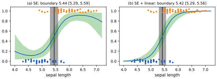
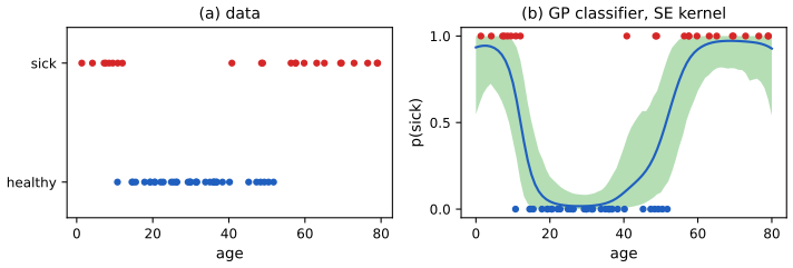
pp. 581–582 With a Bernoulli likelihood the posterior over \(\bm f\) is no longer Gaussian. The book samples the latent function and the kernel parameters jointly by Hamiltonian Monte Carlo on \[ -\mathcal E(\bm f,\bm\theta)=\log\N(\bm f\given\bm 0,\bm K(\bm X,\bm X))+\sum_{n=1}^N\log\Ber(y_n\given\sigma(f_n))+\log p(\bm\theta) \tag{17.55} \] (up to a constant). On the iris flowers (setosa against versicolor from sepal length) with an SE kernel and a \(\mathrm{Ga}(2,0.5)\) prior on \(\ell\), the predicted probability drifts back to \(\frac12\) away from the data; adding a linear kernel \((x-c)(x'-c)\) (17.56), scaled by \(\tau\), \[ \kern(x,x')=\tau(x-c)(x'-c)+\exp\Big(-\frac{(x-x')^2}{2\ell^2}\Big), \tag{17.57} \] encodes a monotone trend and removes the artefact (Figure 17.10). Unlike logistic regression, the GP also fits non-monotone patterns from few data (Figure 17.11).
Filling the gap 17.10: the posterior over the latent function, why the SE classifier returns to \(\frac12\), and the sampler used here pp. 581–582, (17.55)–(17.57)
Derivation
The posterior over \(\bm f\) is log-concave. For fixed \(\bm\theta\), \[ -\log p(\bm f\given\bm y,\bm\theta)=\frac12\bm f^\T\bm K^{-1}\bm f+\sum_n\log(1+e^{-\tilde y_nf_n})+\const \]. The Hessian is \(\bm K^{-1}+\bm W\) with \(\bm W=\diag(\sigma(f_n)(1-\sigma(f_n)))\succ\bm 0\), positive definite: the negative log posterior is strictly convex, so it has a unique mode, which is what the Laplace approximation of the companion course expands around (Bayesian and Probabilistic ML, gap 6.16). Jointly in \((\bm f,\bm\theta)\) there is no such guarantee.
Return to one half. With the SE kernel, \(\kern(x,x_n)\to0\) as \(|x-x_n|\to\infty\) for every \(n\), so \(f(x)\) becomes independent of \(\bm f_X\) and its posterior reverts to the prior \(\N(0,\sigma_f^2)\). Because this law is symmetric and \(\sigma(-a)=1-\sigma(a)\), \(\E[\sigma(f(x))]=\frac12\) exactly: far from the data the classifier says "don't know". With the linear term (17.57), \(f(x)=\beta(x-c)+g(x)\) with \(\beta\sim\N(0,\tau)\) and \(g\) an SE process; the data pin \(\beta\) to positive values, and as \(x\) moves away from the data \(g\) reverts to its prior while \(\beta(x-c)\) keeps growing, so \(p(y=1\given x)\to1\) on one side and \(0\) on the other.
The sampler. Instead of HMC the code writes \(\bm f=\bm L_{\bm\theta}\bm\nu\) with \(\bm L_{\bm\theta}\) the Cholesky factor of the kernel matrix at the training and plotting points and \(\bm\nu\sim\N(\bm 0,\bm I)\), and alternates (i) an elliptical slice sampling update of \(\bm\nu\) (Murray, Adams and MacKay, 2010), which proposes points on the ellipse \(\bm\nu\cos a+\bm\nu'\sin a\) through the current state and a fresh prior draw and shrinks the angle bracket until the likelihood exceeds a uniform threshold, leaving \(\N(\bm\nu\given\bm 0,\bm I)\prod_n\Ber(y_n\given\sigma(f_n))\) invariant without any tuning; and (ii) a random-walk Metropolis update of the unconstrained \(\bm\theta\) (log length scale, log scale, offset) with \(\bm\nu\) held fixed, which is valid for the same joint target and mixes better than updating \(\bm\theta\) with \(\bm f\) fixed. On a one-point problem the sampler reproduces the posterior mean of \(\sigma(f)\) computed by quadrature (0.634 against 0.637 from 40000 draws). \(\square\)
See also: Bayesian and Probabilistic ML, 6.4.5–6.4.6 GP classification and the Laplace approximation; the GP classification demo.
17.2.8 Connections with deep learning
p. 582 A network with one infinitely wide layer of RBF units and random output weights is a GP with an RBF kernel; more generally, infinitely wide networks of many architectures are GPs, and the neural tangent kernel (Jacot et al., 2018) describes the training dynamics of wide networks.
Filling the gap 17.11: an infinitely wide layer of RBF units is a GP with an RBF kernel p. 582
Derivation
Let \(f_H(x)=H^{-1/2}\sum_{h=1}^Hv_h\phi(x;\mu_h)\) with \(\phi(x;\mu)=\exp(-(x-\mu)^2/(2s^2))\), independent output weights \(v_h\sim\N(0,\sigma_v^2)\) and independent centres \(\mu_h\) with density \(q\). For fixed inputs \(x_1,\dots,x_M\), the vector \((f_H(x_m))_m\) is \(H^{-1/2}\) times a sum of \(H\) i.i.d. zero-mean vectors with covariance \(C(x,x')=\sigma_v^2\E_\mu[\phi(x;\mu)\phi(x';\mu)]\) (finite, since \(0\le\phi\le1\)). By the multivariate central limit theorem it converges in law to \(\N(\bm 0,[C(x_i,x_j)])\): the limit is a GP with kernel \(C\). Completing the square, \[ (x-\mu)^2+(x'-\mu)^2=2\Big(\mu-\frac{x+x'}2\Big)^2+\frac{(x-x')^2}2,\qquad \int\phi(x;\mu)\phi(x';\mu)\,\d\mu=\sqrt\pi\,s\,\exp\Big(-\frac{(x-x')^2}{4s^2}\Big). \] So if the centres are spread uniformly over an interval \([-B,B]\) (density \(1/2B\)) and \(\sigma_v^2\) is scaled with \(B\), then as \(B\to\infty\) the covariance at fixed \(x,x'\) tends to a multiple of the SE kernel with length scale \(\ell=\sqrt2\,s\) (in \(D\) dimensions the factor is \((\sqrt\pi s)^D\)); the integral identity is confirmed by quadrature to \(10^{-9}\). With Gaussian-distributed centres instead, the same computation gives a non-stationary kernel (Williams, 1998). Neal's general argument for one hidden layer is in the companion course: Bayesian and Probabilistic ML, Result 6.5. \(\square\)
17.2.9 Scaling GPs to large datasets
pp. 582–584 Exact GP inference costs \(O(N^3)\) time and \(O(N^2)\) memory. Three remedies.
17.2.9.1 Sparse (inducing-point) approximations. Summarise the \(N\) training points by \(M\ll N\) inducing points \(\bm Z\) and their function values \(\bm f_Z\); predictions use \(p(f_*\given\bm f_Z)\) instead of \(p(f_*\given\bm f_X)\), at cost \(O(NM^2)\). Learning \(\bm Z\) and the law of \(\bm f_Z\) is done rigorously by variational inference (in the book's sequel).
Filling the gap 17.12: the simplest inducing-point approximation and its \(O(NM^2)\) cost p. 583
Derivation
Replace the GP by the finite-rank process \(\tilde f(\bm x)=\bm k_Z(\bm x)^\T\bm K_{ZZ}^{-1}\bm f_Z\) with \(\bm f_Z\sim\N(\bm 0,\bm K_{ZZ})\), \(\bm k_Z(\bm x)=[\kern(\bm x,\bm z_m)]_m\): the posterior mean of \(f(\bm x)\) given \(\bm f_Z\), used as if it were the function (the "subset of regressors" approximation). Its kernel is the Nyström kernel \(\tilde\kern(\bm x,\bm x')=\bm k_Z(\bm x)^\T\bm K_{ZZ}^{-1}\bm k_Z(\bm x')\), which agrees with \(\kern\) whenever one argument is an inducing point. This is Bayesian linear regression with features \(\phi(\bm x)=\bm k_Z(\bm x)\) and prior covariance \(\bm\Sigma_w=\bm K_{ZZ}^{-1}\) (write \(\bm f_Z=\bm K_{ZZ}\bm w\)), so by gap 17.8 the predictive mean can be computed in weight space: \[ \tilde\mu_*=\bm k_Z(\bm x_*)^\T\big(\sigma_y^2\bm K_{ZZ}+\bm K_{ZX}\bm K_{XZ}\big)^{-1}\bm K_{ZX}\bm y , \] which needs \(\bm K_{ZX}\bm K_{XZ}\) (\(O(NM^2)\)) and an \(M\times M\) solve (\(O(M^3)\)), instead of the \(N\times N\) solve of the function-space formula with \(\tilde\kern\). The two formulas agree numerically. The price is a degenerate prior: far from the inducing points \(\tilde\kern(\bm x,\bm x)\to0\), so this approximation becomes overconfident there, which is what the more careful approximations (FITC, the variational method of the sequel; Quiñonero-Candela and Rasmussen, 2005) correct. \(\square\)
17.2.9.2 Exploiting parallelisation and kernel matrix structure. Krylov-subspace methods (conjugate gradients, Lanczos) solve \(\bm K_\sigma\bm\alpha=\bm y\) and estimate \(\log|\bm K_\sigma|\) using only matrix-vector products, which parallelise well on GPUs and exploit structure (Toeplitz, Kronecker, sparsity). Conjugate gradients on an \(N\times N\) PD system terminates in at most \(N\) steps in exact arithmetic and, in practice, reaches useful accuracy in far fewer when \(\bm K_\sigma\) is well conditioned.
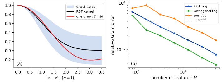
17.2.9.3 Random feature approximation. For the RBF kernel with bandwidth \(\sigma\), \[ \kern(\bm x,\bm x')\approx\phi(\bm x)^\T\phi(\bm x'),\qquad \phi(\bm x)=\frac1{\sqrt T}\big[\sin(\bm\Omega\bm x),\cos(\bm\Omega\bm x)\big],\quad\bm\Omega\in\R^{T\times D},\ \Omega_{td}\sim\N(0,\sigma^{-2}), \tag{17.58–17.60} \] with \(M=2T\) features: random Fourier features (Rahimi and Recht, 2007). A GP or kernel ridge regression on these features costs \(O(NM^2+M^3)\) instead of \(O(N^3)\). Positive random features (17.61) use \(\exp(\bm\omega_m^\T\bm x)\) instead of sines and cosines; orthogonal random features draw the rows of \(\bm\Omega\) orthogonal, which lowers the variance (Yu et al., 2016). Fastfood replaces \(\bm\Omega\) by products of Hadamard and diagonal matrices: \(O(M)\) memory and \(O(M\log D)\) time. Extreme learning machines are one-hidden-layer networks \(f(\bm x)=\bm W h(\bm\Omega\bm x)\) (17.62) with random fixed \(\bm\Omega\) and only \(\bm W\) trained, i.e. linear models on random features.
Filling the gap 17.13: random Fourier features are unbiased, with variance \((1-k^2)^2/(2T)\); positive and orthogonal features pp. 583–584, (17.58)–(17.62)
Derivation
Unbiasedness. For \(\bm\omega\sim\N(\bm 0,\sigma^{-2}\bm I)\), the characteristic function of a Gaussian gives \(\E[e^{i\bm\omega^\T\bm\delta}]=e^{-\|\bm\delta\|^2/(2\sigma^2)}\); taking real parts, \(\E[\cos(\bm\omega^\T\bm\delta)]=\kern(\bm\delta)\) (Bochner's theorem, gap 17.3, with the spectral density of the SE kernel). Since \(\sin a\sin b+\cos a\cos b=\cos(a-b)\), \[ \phi(\bm x)^\T\phi(\bm x')=\frac1T\sum_{t=1}^T\cos\big(\bm\omega_t^\T(\bm x-\bm x')\big), \] an average of \(T\) i.i.d. unbiased estimates of \(\kern(\bm x,\bm x')\). So the approximation is unbiased for every \(M\); what decreases with \(M\) is its variance (the book says "the bias decreases").
Exact variance. With \(k=\kern(\bm\delta)\), \[ \E[\cos^2(\bm\omega^\T\bm\delta)]=\frac12(1+\E\cos(2\bm\omega^\T\bm\delta))=\frac12(1+\kern(2\bm\delta)) \], and for the SE kernel \(\kern(2\bm\delta)=k^4\). Hence \(\var[\cos(\bm\omega^\T\bm\delta)]=\frac12(1+k^4)-k^2=\frac12(1-k^2)^2\) and \[ \var\big[\phi(\bm x)^\T\phi(\bm x')\big]=\frac{(1-k^2)^2}{2T}. \] The error vanishes for identical points (\(k=1\)), is largest, \(1/(2T)\), for distant ones, and the Gram-matrix error falls like \(M^{-1/2}\) (Figure 17.S1). 20000 simulated estimates give variance 0.011257 against the formula's 0.011173. Uniform error bounds over a compact set (Rahimi and Recht, 2007) add a \(\sqrt{D\log(\cdot)}\) factor.
Positive features: a correction to (17.61). For \(\bm\omega\sim\N(\bm 0,\bm I)\) the Gaussian moment generating function gives \[ \E[e^{\bm\omega^\T\bm x}e^{\bm\omega^\T\bm y}]=e^{\|\bm x+\bm y\|^2/2}=e^{\|\bm x\|^2/2+\|\bm y\|^2/2+\bm x^\T\bm y} \]. With the prefactor \(e^{-\|\bm x\|^2/2}\) of (17.61) the estimate is therefore of \(e^{\bm x^\T\bm y}\), the "softmax" kernel used for attention (Choromanski et al., 2021), not of the RBF kernel. Since \(e^{-\|\bm x-\bm y\|^2/2}=e^{-\|\bm x\|^2/2-\|\bm y\|^2/2+\bm x^\T\bm y}\), the RBF kernel needs the prefactor \(e^{-\|\bm x\|^2}\): \(\phi(\bm x)=M^{-1/2}e^{-\|\bm x\|^2}(e^{\bm\omega_m^\T\bm x})_m\) (with bandwidth \(\sigma\), replace \(\bm x\) by \(\bm x/\sigma\)). Monte Carlo confirms both statements to \(10^{-3}\). The variance of one term is \(e^{4\bm x^\T\bm y}-k^2\), which for \(\bm x=\bm y\) is \(e^{4\|\bm x\|^2}-1\): positive features are excellent near the origin and useless far from it (demo, preset 5).
Orthogonal features. If \(\bm G\) has i.i.d. \(\N(0,1)\) entries, the orthogonal factor \(\bm Q\) of its QR (Gram-Schmidt) decomposition is uniformly (Haar) distributed, so each row of \(\bm Q\) is a uniform unit vector; multiplying row \(i\) by an independent \(\chi_D\) length makes it exactly \(\N(\bm 0,\bm I)\). Each frequency therefore has the same marginal law as before (unbiasedness is kept) while the frequencies within a block are negatively dependent, which reduces the variance (Yu et al., 2016). Numerically, for \(D=16\) and \(M=64\) the mean relative Gram error over 8 draws is 0.384 against 0.479 for i.i.d. features (Figure 17.S1b).
Costs and normalisation. Ridge regression on \(M\) features forms \(\bm\Phi^\T\bm\Phi\) at cost \(O(NM^2)\), so the total is \(O(NM^2+M^3)\), not the \(O(NM+M^3)\) printed in the text. And with \(M=2T\) features \([\sin,\cos]\), the normalisation \(\sqrt{1/M}\) in (17.62) gives \(\frac12\kern\); the consistent factor is \(1/\sqrt T=\sqrt{2/M}\), as in (17.59). \(\square\)
17.3 Support vector machines (SVMs)
p. 585 A support vector machine predicts with \(f(\bm x)=\sum_{i=1}^N\alpha_i\kern(\bm x,\bm x_i)\) (17.63) (plus a bias), where constraints make most \(\alpha_i\) zero; the training points with \(\alpha_i\ne0\) are the support vectors. It is not probabilistic: it estimates a decision rule, not a distribution.
17.3.1 Large margin classifiers
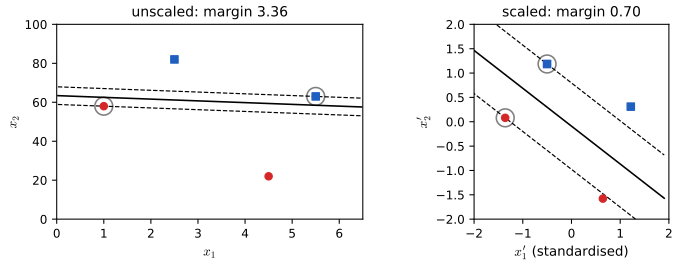
pp. 585–587 For a linear rule \(h(\bm x)=\sign(f(\bm x))\), \(f(\bm x)=\bm w^\T\bm x+w_0\) (17.64), with labels \(\tilde y\in\{-1,+1\}\), the signed distance of \(\bm x\) from the boundary is \(r=f(\bm x)/\|\bm w\|\) (decompose \(\bm x=\bm x_\perp+r\bm w/\|\bm w\|\) and use \(f(\bm x_\perp)=0\), (17.65)–(17.66)). Among the separating hyperplanes, the one of maximum margin (the largest distance to the closest point, Figure 17.12, a sketch) solves \[ \max_{\bm w,w_0}\frac1{\|\bm w\|}\min_{n}\tilde y_n(\bm w^\T\bm x_n+w_0) \tag{17.67} \] and, after fixing the scale so that the closest point has \(\tilde y_nf_n=1\), \[ \min_{\bm w,w_0}\tfrac12\|\bm w\|^2\quad\text{s.t.}\quad\tilde y_n(\bm w^\T\bm x_n+w_0)\ge1,\ n=1:N. \tag{17.68} \] Because the margin is a Euclidean distance, the inputs should be standardised first (Figure 17.14).
Filling the gap 17.14: why (17.67) and (17.68) have the same solution, and why it is unique pp. 586–587
Derivation
Assume the data are linearly separable, so some \((\bm w,w_0)\) has \(\tilde y_nf_n>0\) for all \(n\). The objective of (17.67), \(g(\bm w,w_0)=\min_n\tilde y_n(\bm w^\T\bm x_n+w_0)/\|\bm w\|\), is invariant under \((\bm w,w_0)\mapsto(c\bm w,cw_0)\), \(c>0\). Every separating \((\bm w,w_0)\) can therefore be rescaled so that \(\min_n\tilde y_nf_n=1\); on this set \(g=1/\|\bm w\|\), and the constraint set \(\{\tilde y_nf_n\ge1\ \forall n\}\) contains it and has the same supremum of \(1/\|\bm w\|\) (a point with \(\min_n\tilde y_nf_n=m>1\) can be scaled down by \(m\), which increases \(1/\|\bm w\|\)). Maximising \(1/\|\bm w\|\) is minimising \(\frac12\|\bm w\|^2\): (17.68). Existence and uniqueness. The feasible set of (17.68) is a nonempty closed convex polyhedron and \(\frac12\|\bm w\|^2\) is continuous and coercive in \(\bm w\), so a minimiser exists; strict convexity in \(\bm w\) makes \(\hat{\bm w}\) unique. Given \(\hat{\bm w}\), the feasible \(w_0\) form an interval, and at the optimum both classes have a point with \(\tilde y_nf_n=1\) (otherwise \(w_0\) could be shifted to make all constraints slack, and then \(\bm w\) shrunk), which pins \(\hat w_0\) down. Companion proofs: Bayesian and Probabilistic ML, gap 7.1 and Result 7.1. \(\square\)
17.3.2 The dual problem
pp. 587–589 (17.68) is a quadratic program in the \(D+1\) variables \((\bm w,w_0)\) with \(N\) linear constraints. With multipliers \(\bm\alpha\ge\bm 0\) the Lagrangian is \[ L(\bm w,w_0,\bm\alpha)=\tfrac12\bm w^\T\bm w-\sum_{n=1}^N\alpha_n\big(\tilde y_n(\bm w^\T\bm x_n+w_0)-1\big), \tag{17.69} \] and stationarity in \(\bm w\) and \(w_0\) gives \(\hat{\bm w}=\sum_n\hat\alpha_n\tilde y_n\bm x_n\) and \(\sum_n\hat\alpha_n\tilde y_n=0\) (17.71)–(17.74). Substituting, \[ \max_{\bm\alpha}\ \sum_n\alpha_n-\frac12\sum_{i,j}\alpha_i\alpha_j\tilde y_i\tilde y_j\bm x_i^\T\bm x_j\quad\text{s.t.}\ \sum_n\alpha_n\tilde y_n=0,\ \alpha_n\ge0 , \tag{17.75–17.77} \] a QP in \(N\) variables, solved by specialised methods such as sequential minimal optimisation (SMO, Platt 1998). The KKT conditions \[ \alpha_n\ge0,\qquad\tilde y_nf(\bm x_n)-1\ge0,\qquad\alpha_n\big(\tilde y_nf(\bm x_n)-1\big)=0 \tag{17.78–17.80} \] say that \(\alpha_n>0\) only for points on the margin, \(\tilde y_nf(\bm x_n)=1\): the support vectors \(\mathcal S\). Prediction uses \(f(\bm x)=\sum_{n\in\mathcal S}\alpha_n\tilde y_n\bm x_n^\T\bm x+\hat w_0\) (17.81), with \(\hat w_0=\frac1{|\mathcal S|}\sum_{n\in\mathcal S}(\tilde y_n-\hat{\bm w}^\T\bm x_n)\) (17.82).
Filling the gap 17.15: the dual (17.77), why min-max equals max-min, and the KKT conditions pp. 587–589
Derivation
The dual function. For fixed \(\bm\alpha\ge\bm 0\), \(L\) is a strictly convex quadratic in \(\bm w\) plus the linear term \(-w_0\sum_n\alpha_n\tilde y_n\). Its infimum over \(w_0\in\R\) is \(-\infty\) unless \(\sum_n\alpha_n\tilde y_n=0\); then the infimum over \(\bm w\) is at \(\bm w=\sum_n\alpha_n\tilde y_n\bm x_n\) (17.73), and substituting, \(\frac12\|\bm w\|^2-\bm w^\T\bm w-0+\sum_n\alpha_n\) (17.75)–(17.76), which is (17.77). So the dual problem is "maximise (17.77) subject to \(\sum\alpha_n\tilde y_n=0,\ \bm\alpha\ge\bm 0\)".
No duality gap. Weak duality, \(g(\bm\alpha)\le\frac12\|\bm w\|^2\) for every dual-feasible \(\bm\alpha\) and primal-feasible \((\bm w,w_0)\), is immediate (the subtracted terms are nonnegative). For a convex quadratic program with linear constraints that is feasible and bounded below, strong duality holds and the dual optimum is attained (no Slater condition is needed for affine constraints; see Section 8.5.2). Therefore the saddle point (17.70) exists, and the KKT conditions are necessary and sufficient for optimality: primal feasibility (17.79), dual feasibility (17.78), stationarity (17.73)–(17.74) and complementary slackness (17.80).
Support vectors lie on the margin. By (17.80), \(\alpha_n>0\) forces \(\tilde y_nf(\bm x_n)=1\), i.e. distance \(1/\|\hat{\bm w}\|\) from the boundary: the point is on the margin hyperplane, not on the decision boundary \(f=0\) as the text says. The solution depends only on \(\mathcal S\): removing any other point and refitting gives the same classifier.
The bias. For \(n\in\mathcal S\), \(\tilde y_n(\hat{\bm w}^\T\bm x_n+\hat w_0)=1\); multiplying by \(\tilde y_n\) (with \(\tilde y_n^2=1\)) gives \(\hat w_0=\tilde y_n-\hat{\bm w}^\T\bm x_n\) for every support vector, so the average (17.82) is the same number in exact arithmetic and simply reduces rounding error (on the data of Figure 17.14, 0.101628 by both routes). Companion results: Elements of Statistical Learning, Result 12.1; Bayesian and Probabilistic ML, Results 7.2–7.4. \(\square\)
17.3.3 Soft margin classifiers
pp. 589–590 For non-separable data, slack variables \(\xi_n\ge0\) relax the constraints to \(\tilde y_nf_n\ge1-\xi_n\): \[ \min_{\bm w,w_0,\bm\xi}\ \tfrac12\|\bm w\|^2+C\sum_{n=1}^N\xi_n\quad\text{s.t.}\ \xi_n\ge0,\ \tilde y_n(\bm x_n^\T\bm w+w_0)\ge1-\xi_n . \tag{17.83} \] The dual has the same objective as (17.77), \[ \mathcal L(\bm\alpha)=\sum_i\alpha_i-\frac12\sum_{i,j}\alpha_i\alpha_j\tilde y_i\tilde y_j\bm x_i^\T\bm x_j,\qquad0\le\alpha_n\le C,\quad\sum_n\alpha_n\tilde y_n=0, \tag{17.85–17.87} \] with the box constraint as the only change. Points with \(\alpha_n=0\) are outside the margin; \(0<\alpha_n<C\) on it; \(\alpha_n=C\) inside it or misclassified. The bias is averaged over the points on the margin, \(\mathcal M=\{n:0<\alpha_n<C\}\) (17.88). In the \(\nu\)-SVM (Schölkopf et al., 2000) the parameter \(\nu\in(0,1]\) replaces \(C\): \[ \max_{\bm\alpha}-\frac12\sum_{i,j}\alpha_i\alpha_j\tilde y_i\tilde y_j\bm x_i^\T\bm x_j\quad\text{s.t.}\ 0\le\alpha_n\le\frac1N,\ \sum_n\alpha_n\tilde y_n=0,\ \sum_{n=1}^N\alpha_n\ge\nu , \tag{17.89–17.92} \] and \(\nu\) bounds the fraction of margin errors from above and the fraction of support vectors from below.
Filling the gap 17.16: the soft-margin dual, the box \(0\le\alpha_n\le C\), and the three kinds of points pp. 589–590, (17.83)–(17.88)
Derivation
Dual. The Lagrangian (17.84) has multipliers \(\alpha_n\ge0\) for the margin constraints and \(\mu_n\ge0\) for \(\xi_n\ge0\). Stationarity: \(\partial_{\bm w}\): \(\bm w=\sum\alpha_n\tilde y_n\bm x_n\); \(\partial_{w_0}\): \(\sum\alpha_n\tilde y_n=0\); \(\partial_{\xi_n}\): \(C-\alpha_n-\mu_n=0\). Substituting, every term in \(\bm\xi\) cancels (\(C\xi_n-\alpha_n\xi_n-\mu_n\xi_n=0\)) and the dual objective is (17.85), the same as before. The only trace of \(\bm\xi\) is the constraint \(\mu_n=C-\alpha_n\ge0\), i.e. \(\alpha_n\le C\): the box (17.86). Strong duality holds as in gap 17.15.
Three kinds of points (complementary slackness \(\alpha_n(\tilde y_nf_n-1+\xi_n)=0\) and \(\mu_n\xi_n=0\)). If \(\alpha_n=0\): \(\mu_n=C>0\), so \(\xi_n=0\) and \(\tilde y_nf_n\ge1\) (on or outside the margin, correct side). If \(0<\alpha_n<C\): \(\mu_n>0\) gives \(\xi_n=0\), and \(\alpha_n>0\) gives \(\tilde y_nf_n=1-\xi_n=1\): exactly on the margin. If \(\alpha_n=C\): \(\mu_n=0\), so \(\xi_n\ge0\) is free and \(\tilde y_nf_n=1-\xi_n\le1\): inside the margin, correctly classified if \(\xi_n\le1\), misclassified if \(\xi_n>1\). Hence \(\sum_n\xi_n\ge\#\{n:\xi_n>1\}\ge\#\{\)training errors\(\}\). The bias (17.88) follows from \(\tilde y_nf_n=1\) on \(\mathcal M\) as in the hard-margin case; if \(\mathcal M\) is empty, \(\hat w_0\) is only pinned to an interval and any point of it is optimal.
Checked numerically. The SMO solver in the code (second-order working-set selection, Fan, Chen and Lin, 2005) reaches the same dual objective and support set as libsvm at all five \((\gamma,C)\) tried; the KKT pattern above holds to \(10^{-4}\); and the primal (17.83) equals the dual (17.85) at the solution. Companion proofs: Bayesian and Probabilistic ML, Result 7.6, Elements of Statistical Learning, Result 12.2; the SMO step is derived in Bayesian and Probabilistic ML, gap 7.3. \(\square\)
Filling the gap 17.17: Result 17.5 (the \(\nu\)-SVM: its primal, its dual (17.89)–(17.92), and the \(\nu\)-property) p. 590
Derivation
Primal. The \(\nu\)-SVM makes the margin width a variable \(\rho\ge0\): \[ \min_{\bm w,w_0,\bm\xi,\rho}\ \tfrac12\|\bm w\|^2-\nu\rho+\frac1N\sum_n\xi_n\quad\text{s.t.}\ \tilde y_n(\bm w^\T\bm x_n+w_0)\ge\rho-\xi_n,\ \xi_n\ge0,\ \rho\ge0 . \] Dual. With multipliers \(\alpha_n,\mu_n,\delta\ge0\): \(\partial_{\bm w}\): \(\bm w=\sum\alpha_n\tilde y_n\bm x_n\); \(\partial_{w_0}\): \(\sum\alpha_n\tilde y_n=0\); \(\partial_{\xi_n}\): \(\frac1N-\alpha_n-\mu_n=0\), so \(0\le\alpha_n\le\frac1N\); \(\partial_\rho\): \(-\nu+\sum\alpha_n-\delta=0\), so \(\sum\alpha_n=\nu+\delta\ge\nu\). Substituting leaves only \(-\frac12\|\sum\alpha_n\tilde y_n\bm x_n\|^2\): this is (17.89)–(17.92), with the upper limit of the sum in (17.92) equal to \(N\) (the book prints \(M\)).
Result 17.5 (\(\nu\)-property). If the optimal \(\rho>0\), then (fraction of margin errors) \(\le\nu\le\) (fraction of support vectors), where a margin error is a point with \(\xi_n>0\). Proof. \(\rho>0\) and complementary slackness \(\delta\rho=0\) give \(\delta=0\), so \(\sum_n\alpha_n=\nu\). A margin error has \(\xi_n>0\), so \(\mu_n=0\) and \(\alpha_n=\frac1N\); hence \(\frac{\#\text{margin errors}}N=\sum_{\text{m.e.}}\alpha_n\le\sum_n\alpha_n=\nu\). Every \(\alpha_n\le\frac1N\) and only support vectors have \(\alpha_n>0\), so \(\nu=\sum_n\alpha_n\le\frac{\#\text{SV}}N\). \(\square\) The bounds are on fractions, not numbers as the text says. On the moons data, \(\nu=0.2\) gives fractions 0.17 and 0.23, \(\nu=0.5\) gives 0.46 and 0.52. Companion: Bayesian and Probabilistic ML, Result 7.7.
17.3.4 The kernel trick
p. 590 The dual and the prediction involve the inputs only through inner products \(\bm x^\T\bm x'\). Replacing them by a Mercer kernel gives \[ f(\bm x)=\sum_{n\in\mathcal S}\alpha_n\tilde y_n\kern(\bm x_n,\bm x)+\hat w_0,\qquad\hat w_0=\frac1{|\mathcal S|}\sum_{i\in\mathcal S}\Big(\tilde y_i-\sum_{j\in\mathcal S}\hat\alpha_j\tilde y_j\kern(\bm x_j,\bm x_i)\Big), \tag{17.93, 17.94} \] a linear classifier in the feature space of \(\kern\), nonlinear in the inputs, computed without ever forming the features.
Filling the gap 17.18: why kernelising is legitimate: the RKHS and Result 17.4 (the representer theorem) p. 590
Derivation
The feature space. Given a PSD kernel, let \(\mathcal H_0\) be the finite combinations \(f=\sum_ia_i\kern(\cdot,\bm x_i)\) with \[ \langle\sum_ia_i\kern(\cdot,\bm x_i),\sum_jb_j\kern(\cdot,\bm z_j)\rangle=\sum_{ij}a_ib_j\kern(\bm x_i,\bm z_j) \]. This is well defined: it equals \(\sum_jb_jf(\bm z_j)\) and also \(\sum_ia_ig(\bm x_i)\) for \(f=\sum_ia_i\kern(\cdot,\bm x_i)\), \(g=\sum_jb_j\kern(\cdot,\bm z_j)\), so it does not depend on how \(f\) and \(g\) are written; it is symmetric, and \(\langle f,f\rangle=\bm a^\T\bm K\bm a\ge0\) by (17.1). The reproducing property \(\langle f,\kern(\cdot,\bm x)\rangle=f(\bm x)\) holds by construction, and Cauchy-Schwarz gives \(|f(\bm x)|\le\|f\|\sqrt{\kern(\bm x,\bm x)}\), so \(\|f\|=0\) implies \(f\equiv0\): \(\langle\cdot,\cdot\rangle\) is an inner product. Completing \(\mathcal H_0\) gives the reproducing kernel Hilbert space \(\Hk\) (Aronszajn, 1950), with the feature map \(\phi(\bm x)=\kern(\cdot,\bm x)\) and \(\langle\phi(\bm x),\phi(\bm x')\rangle=\kern(\bm x,\bm x')\). A kernel SVM is the linear SVM in \(\Hk\): \(f=g+w_0\) with \(g\in\Hk\) and \(\|\bm w\|^2\) replaced by \(\|g\|^2_{\Hk}\).
Result 17.4 (representer theorem; Kimeldorf and Wahba, 1971). Let \(\ell\) be any loss and \(\lambda>0\). Every minimiser over \(g\in\Hk\), \(w_0\in\R\) of \(\sum_n\ell(\tilde y_n,g(\bm x_n)+w_0)+\lambda\|g\|^2_{\Hk}\) has the form \(g=\sum_{n=1}^N\alpha_n\kern(\cdot,\bm x_n)\). Proof. Write \(g=g_\parallel+g_\perp\) with \(g_\parallel\) in the span \(V\) of \(\kern(\cdot,\bm x_1),\dots,\kern(\cdot,\bm x_N)\) and \(g_\perp\perp V\) (orthogonal projection onto the finite-dimensional, hence closed, \(V\)). By the reproducing property \[ g(\bm x_n)=\langle g,\kern(\cdot,\bm x_n)\rangle=\langle g_\parallel,\kern(\cdot,\bm x_n)\rangle=g_\parallel(\bm x_n) \]: the data term does not see \(g_\perp\). But \(\|g\|^2=\|g_\parallel\|^2+\|g_\perp\|^2\), so replacing \(g\) by \(g_\parallel\) strictly decreases the objective unless \(g_\perp=0\). \(\square\) With the hinge loss this is the kernel SVM (17.93); with the squared loss, kernel ridge regression (Section 17.3.9); with the log loss, kernel logistic regression (the L2VM of Section 17.4). In all cases \(\|g\|^2_{\Hk}=\bm\alpha^\T\bm K\bm\alpha\), so the infinite-dimensional problem becomes an \(N\)-dimensional one. Companion results: Elements of Statistical Learning, Result 12.7 and Section 5.8.
17.3.5 Converting SVM outputs into probabilities
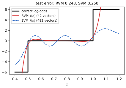
p. 591 Platt scaling treats the SVM score as a log-odds after an affine map, \[ p(y=1\given\bm x,\bm\theta)=\sigma(af(\bm x)+b), \tag{17.95} \] with \(a,b\) fitted by maximum likelihood on a separate validation set (on the training set it overfits). The result is often poorly calibrated, because nothing in SVM training makes \(f\) a log-odds. Tipping's example: \(p(x\given y=0)=\mathrm{Unif}(0,1)\), \(p(x\given y=1)=\mathrm{Unif}(0.5,1.5)\), equal priors; the true log-odds is \(-\infty\) below 0.5, 0 on \([0.5,1]\) and \(+\infty\) above 1, and the Bayes error is 25%. Both an RVM and an SVM reach about that error, but only the RVM's output resembles the log-odds (Figure 17.15).
17.3.6 Connection with logistic regression
pp. 591–592 At the optimum of (17.83), \(\xi_n=\max(0,1-\tilde y_nf(\bm x_n))\), so the soft-margin SVM minimises \[ \mathcal L(\bm w)=\sum_{n=1}^N\ell_{\rm hinge}(\tilde y_n,f(\bm x_n))+\lambda\|\bm w\|^2,\quad\lambda=(2C)^{-1},\qquad\ell_{\rm hinge}(\tilde y,\eta)=\max(0,1-\tilde y\eta), \tag{17.96, 17.97} \] while penalised logistic regression minimises the same with the log loss \(\ell_{ll}(\tilde y,\eta)=\log(1+e^{-\tilde y\eta})\) (17.98, 17.99). The hinge loss is piecewise linear (non-differentiable at \(\tilde y\eta=1\), where a subgradient is used) and exactly zero for \(\tilde y\eta\ge1\), which is what produces sparse solutions. Both are convex surrogates for the 0-1 loss \(\ind(\tilde y\hat y<0)\) (17.100).
Filling the gap 17.19: the hinge form, upper bounds on the 0-1 loss, and why the SVM output is not a log-odds pp. 591–592, (17.95)–(17.100)
Derivation
The hinge form. For fixed \((\bm w,w_0)\), (17.83) is minimised over each \(\xi_n\) separately: \(\xi_n\ge0\) and \(\xi_n\ge1-\tilde y_nf_n\), with a positive cost, so \(\xi_n=\max(0,1-\tilde y_nf_n)\). Then \[ \frac12\|\bm w\|^2+C\sum_n\xi_n=C\big[\sum_n\ell_{\rm hinge}+\frac1{2C}\|\bm w\|^2\big] \], which is \(C\) times (17.96) with \(\lambda=1/(2C)\) (checked to machine precision).
Upper bounds. \(\max(0,1-\eta)\ge\ind(\eta<0)\): for \(\eta<0\) the left side exceeds 1, otherwise it is \(\ge0\). The log loss in natural logarithms is not an upper bound: at \(\eta=0\) it equals \(\log2\approx0.693<1\). Its base-2 version \(\log_2(1+e^{-\eta})\) is (it equals 1 at \(\eta=0\) and is convex and decreasing with slope \(-1/(2\log 2)\) there, hence above the step). The statement "both are convex upper bounds" needs this rescaling.
Population minimisers. Let \(p=\Pr(\tilde y=1\given\bm x)\). The conditional risk of the log loss, \(p\log(1+e^{-\eta})+(1-p)\log(1+e^{\eta})\), has derivative \(-p\sigma(-\eta)+(1-p)\sigma(\eta)=\sigma(\eta)-p\), zero at \(\eta=\log\frac p{1-p}\): logistic regression estimates the log-odds. The hinge risk \(p\max(0,1-\eta)+(1-p)\max(0,1+\eta)\) is piecewise linear in \(\eta\) with slopes \(-1\) (for \(\eta<-1\)), \(1-2p\) (on \([-1,1]\)), \(+1\) (for \(\eta>1\)); it is minimised at \(\eta=\sign(2p-1)\) when \(p\ne\frac12\), and is flat on \([-1,1]\) when \(p=\frac12\). So the SVM estimates the Bayes decision \(\sign(2p-1)\), not \(p\): its output carries no probability beyond the sign. In Tipping's overlap region \(p=\frac12\), every value in \([-1,1]\) is equally good, which is why the SVM in Figure 17.15 wanders between \(\pm1\) there while the RVM, a likelihood-based model, stays near the true log-odds 0. Platt scaling (17.95) is a one-feature logistic regression on \(f\), convex and solved by Newton's method (code: platt); on the training set it overfits because many training scores sit exactly at \(\tilde yf=1\) by construction. Companion results: Elements of Statistical Learning, Result 12.6 (population minimisers) and Bayesian and Probabilistic ML, gap 7.4. \(\square\)
17.3.7 Multi-class classification with SVMs
pp. 592–593 One-versus-the-rest trains \(C\) binary SVMs (class \(c\) against all others) and predicts \(\argmax_cf_c(\bm x)\); its scores are not calibrated against each other, the binary problems are imbalanced (10% positives with 10 classes), and without the argmax some regions would be claimed by several classes or by none (Figure 17.16a, a sketch). One-versus-one trains \(C(C-1)/2\) pairwise SVMs and takes a majority vote, which can tie (Figure 17.16b). Probabilistic multiclass models (softmax over kernel features, Section 17.4) avoid both problems.
17.3.8 How to choose the regularizer C
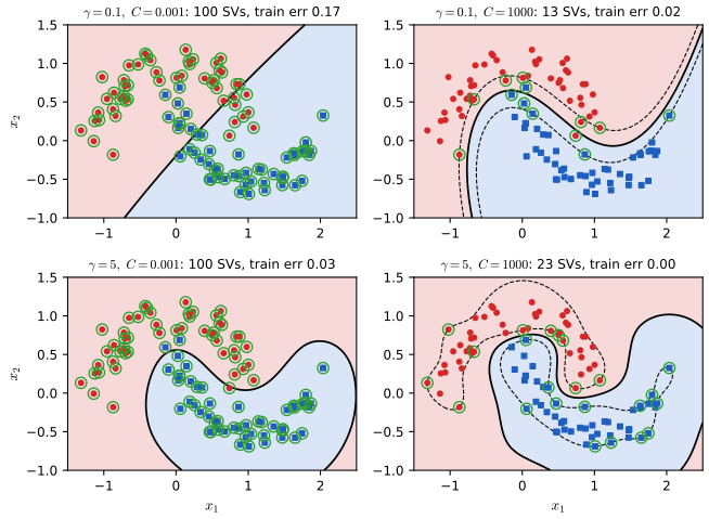
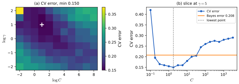
pp. 593–594 \(C\) and the kernel precision \(\gamma=1/(2\sigma^2)\) of the RBF kernel \(\exp(-\gamma\|\bm x-\bm x'\|^2)\) interact strongly: narrow kernels (large \(\gamma\)) need strong regularisation (small \(C\)), wide kernels the opposite (Figure 17.17). The usual recipe is cross-validation on a grid, e.g. \(C\in\{2^{-5},2^{-3},\dots,2^{15}\}\), \(\gamma\in\{2^{-15},\dots,2^3\}\) (Figure 17.18). The whole path of solutions in \(C\) is piecewise linear and can be computed exactly (Hastie et al., 2004).
Filling the gap 17.20: why \(\gamma\) and \(C\) are coupled, and what the regularisation path really does pp. 593–594
Derivation
Wide kernels: only \(\gamma C\) matters. For small \(\gamma\), \(\kern_{ij}=e^{-\gamma d_{ij}^2}=1-\gamma d_{ij}^2+O(\gamma^2)\) with \(d_{ij}^2=\|\bm x_i\|^2+\|\bm x_j\|^2-2\bm x_i^\T\bm x_j\). In the dual quadratic form \(\sum_{ij}\alpha_i\alpha_j\tilde y_i\tilde y_j\kern_{ij}\) the constant 1 contributes \((\sum_i\alpha_i\tilde y_i)^2=0\), and each \(\|\bm x_i\|^2\) term contributes \((\sum_i\alpha_i\tilde y_i\|\bm x_i\|^2)(\sum_j\alpha_j\tilde y_j)=0\), by the constraint (17.87). What remains is \[ 2\gamma\sum_{ij}\alpha_i\alpha_j\tilde y_i\tilde y_j\bm x_i^\T\bm x_j+O(\gamma^2\|\bm\alpha\|^2) \]. With \(\bm\beta=2\gamma\bm\alpha\) the dual becomes \[ \frac1{2\gamma}\big[\sum_n\beta_n-\frac12\sum_{ij}\beta_i\beta_j\tilde y_i\tilde y_j\bm x_i^\T\bm x_j\big] \] with \(0\le\beta_n\le2\gamma C\), up to a relative error \(O(\gamma)\): the dual of a linear SVM with cost \(C'=2\gamma C\). The decision function reduces the same way, \(f(\bm x)=\sum_n\beta_n\tilde y_n\bm x_n^\T\bm x+\const\). So for wide kernels the RBF SVM is a linear SVM whose effective cost is \(2\gamma C\): shrinking \(\gamma\) must be compensated by a proportionally larger \(C\), which is the diagonal valley in Figure 17.18a. (Checked on the moons data with \(2\gamma C=2\): the multipliers \(2\gamma\alpha_n\) differ from those of the linear SVM with \(C'=2\) by at most 0.019 for \(\gamma=10^{-3}\) and 0.003 for \(\gamma=10^{-4}\).)
Narrow kernels memorise. As \(\gamma\to\infty\), \(\bm K\to\bm I\) for distinct inputs and \(\kern(\bm x,\bm x_n)\to0\) away from the data. The dual becomes \(\max\sum\alpha_n-\frac12\|\bm\alpha\|^2\) with the box and \(\sum\alpha_n\tilde y_n=0\); for balanced classes the solution is \(\alpha_n=\min(1,C)\): every point is a support vector and \(f\) is a sum of spikes at the training points plus a constant. Only a small \(C\) (heavy shrinkage of the spikes) gives a sensible fit, and even then generalisation relies on the bias alone far from the data.
The path. In the parametrisation of Hastie et al. (2004), \(\lambda=1/C\) and \(\alpha_n\in[0,1]\) after rescaling. For \(\lambda\) large (small \(C\)) every point is inside the margin with \(\alpha_n=1\) (at the bound); as \(\lambda\) decreases, points leave the margin one at a time and their \(\alpha_n\) move to 0, piecewise linearly in \(\lambda\) (Elements of Statistical Learning, Result 12.8). For separable data the path ends at the hard-margin SVM, which keeps at least one support vector on each side (with no point strictly inside the margin); the book's "no support vectors remain" is not right. \(\square\)
See also: Elements of Statistical Learning, 12.3.5 the path algorithm and its SVM path demo; the SVM demo of Bayesian and Probabilistic ML.
17.3.9 Kernel ridge regression
pp. 594–595 Ridge regression \(\hat{\bm w}=(\bm X^\T\bm X+\lambda\bm I_D)^{-1}\bm X^\T\bm y\) (17.101) can be rewritten with the matrix inversion lemma as \(\bm w=\bm X^\T(\bm X\bm X^\T+\lambda\bm I_N)^{-1}\bm y=\bm X^\T\bm\alpha\) (17.102)–(17.104), so that \(f(\bm x)=\bm w^\T\bm x=\sum_n\alpha_n\bm x_n^\T\bm x\) (17.105); kernelising, \[ f(\bm x)=\sum_{n=1}^N\alpha_n\kern(\bm x_n,\bm x),\qquad\bm\alpha=(\bm K+\lambda\bm I_N)^{-1}\bm y,\qquad f(\bm x)=\bm k^\T(\bm K+\lambda\bm I_N)^{-1}\bm y , \tag{17.106–17.108} \] kernel ridge regression, identical to the GP posterior mean (17.38) with \(\lambda=\sigma_y^2\). The coefficient vector is dense: every training point is used at test time.
Filling the gap 17.21: (17.102)–(17.108) correctly, and kernel ridge regression as a penalised fit in the RKHS pp. 594–595
Derivation
Push-through. \(\bm X^\T(\bm X\bm X^\T+\lambda\bm I_N)=(\bm X^\T\bm X+\lambda\bm I_D)\bm X^\T\); multiplying by the two inverses gives \[ (\bm X^\T\bm X+\lambda\bm I_D)^{-1}\bm X^\T=\bm X^\T(\bm X\bm X^\T+\lambda\bm I_N)^{-1} \] for any \(\lambda>0\). This is (17.102) and defines \(\bm\alpha=(\bm X\bm X^\T+\lambda\bm I_N)^{-1}\bm y\) (17.103). Here \(\bm X\bm X^\T\) is the \(N\times N\) Gram matrix \([\bm x_i^\T\bm x_j]_{ij}\); the book's rewriting of it as "\(\sum_n\bm x_n^\T\bm x_n\)" is a scalar (the sum of squared norms), and with that reading the formula is wrong (checked numerically). In (17.101) the \(\tilde y_n\) should be \(y_n\) (real responses).
Kernelising. \(\bm X\bm X^\T\) and \(\bm X\bm x\) contain the inputs only through inner products, so replacing \(\bm x_i^\T\bm x_j\) by \(\kern(\bm x_i,\bm x_j)\) gives (17.106)–(17.108). Directly in the RKHS: by Result 17.4 the minimiser of \(\|\bm y-\bm g\|^2+\lambda\|g\|^2_{\Hk}\) (with \(\bm g=(g(\bm x_n))_n\)) is \(g=\sum\alpha_n\kern(\cdot,\bm x_n)\), so \(\bm g=\bm K\bm\alpha\) and the objective is \(\|\bm y-\bm K\bm\alpha\|^2+\lambda\bm\alpha^\T\bm K\bm\alpha\). Its gradient is \(2\bm K[(\bm K+\lambda\bm I)\bm\alpha-\bm y]\), which vanishes at \(\bm\alpha=(\bm K+\lambda\bm I)^{-1}\bm y\) (if \(\bm K\) is singular other \(\bm\alpha\) may also vanish it, but all give the same function \(g\)). Comparing with (17.38): the GP posterior mean is this function with \(\lambda=\sigma_y^2\), equal numerically to \(10^{-12}\). The Bayesian reading of \(\lambda\) is the noise variance relative to the prior scale of \(f\). Companion: Elements of Statistical Learning, Result 12.10; ridge regression in Section 11.3. \(\square\)
17.3.10 SVMs for regression
pp. 595–597 In the \(\ell_2\)-regularised empirical risk \(J(\bm w,\lambda)=\lambda\|\bm w\|^2+\sum_n\ell(\tilde y_n,\hat y_n)\) (17.109) the squared loss gives (kernel) ridge regression. The \(\epsilon\)-insensitive loss \[ L_\epsilon(y,\hat y)=\begin{cases}0&|y-\hat y|<\epsilon\\|y-\hat y|-\epsilon&\text{otherwise}\end{cases} \tag{17.110} \] ignores errors smaller than \(\epsilon\) (an "\(\epsilon\)-tube" around the fit, Figure 17.19) and makes the solution sparse. The usual form is \(J=\frac12\|\bm w\|^2+C\sum_nL_\epsilon(\tilde y_n,\hat y_n)\) (17.111); with slacks \(\xi_n^\pm\ge0\) for points above and below the tube, \(\tilde y_n\le f(\bm x_n)+\epsilon+\xi_n^+\), \(\tilde y_n\ge f(\bm x_n)-\epsilon-\xi_n^-\), it is a QP in \(2N+D+1\) variables (17.112)–(17.114), whose solution is \[ \hat{\bm w}=\sum_n\alpha_n\bm x_n,\qquad f(\bm x)=\hat w_0+\sum_{n:\alpha_n\ne0}\alpha_n\kern(\bm x_n,\bm x), \tag{17.115–17.117} \] with \(\alpha_n=0\) for the points strictly inside the tube: support vector regression (Vapnik, Golowich and Smola, 1997). Small \(C\) regularises strongly; small \(\epsilon\) narrows the tube and increases the number of support vectors (Figure 17.20).
Filling the gap 17.22: the SVR dual, the signs of the coefficients, and why points inside the tube drop out pp. 596–597, (17.111)–(17.117)
Derivation
Lagrangian. With multipliers \(\alpha_n^+,\alpha_n^-\ge0\) for the two tube constraints and \(\mu_n^\pm\ge0\) for \(\xi_n^\pm\ge0\): \[ L=\tfrac12\|\bm w\|^2+C\sum_n(\xi_n^++\xi_n^-)-\sum_n\alpha_n^+(\epsilon+\xi_n^++f_n-y_n)-\sum_n\alpha_n^-(\epsilon+\xi_n^--y_n+f_n)-\sum_n(\mu_n^+\xi_n^++\mu_n^-\xi_n^-). \] Stationarity: \(\bm w=\sum_n(\alpha_n^+-\alpha_n^-)\bm x_n\); \(\sum_n(\alpha_n^+-\alpha_n^-)=0\); \(C-\alpha_n^\pm-\mu_n^\pm=0\), so \(0\le\alpha_n^\pm\le C\). Substituting, with \(\beta_n=\alpha_n^+-\alpha_n^-\), the dual is \[ \max\ -\tfrac12\sum_{ij}\beta_i\beta_j\kern(\bm x_i,\bm x_j)-\epsilon\sum_n(\alpha_n^++\alpha_n^-)+\sum_ny_n\beta_n\quad\text{s.t.}\ \sum_n\beta_n=0,\ 0\le\alpha_n^\pm\le C . \] So (17.115) holds with the coefficient \(\beta_n=\alpha_n^+-\alpha_n^-\in[-C,C]\), which is signed: points above the tube get \(\beta_n>0\), points below get \(\beta_n<0\) (Figure 17.23d shows both signs; "\(\alpha_n\ge0\)" in the text is wrong unless \(\alpha_n\) means \(\alpha_n^+\) and \(\alpha_n^-\) separately).
Sparsity from complementary slackness. \(\alpha_n^+(\epsilon+\xi_n^++f_n-y_n)=0\) and \(\alpha_n^-(\epsilon+\xi_n^--y_n+f_n)=0\). If \(|y_n-f_n|<\epsilon\), both brackets are positive (since \(\xi_n^\pm\ge0\)), so \(\alpha_n^+=\alpha_n^-=0\): points strictly inside the tube are not support vectors. Both multipliers cannot be positive at once (that would need \(y_n-f_n=\epsilon+\xi_n^+\) and \(f_n-y_n=\epsilon+\xi_n^-\), adding to \(0=2\epsilon+\xi_n^++\xi_n^-\)), so \(\alpha_n^+\alpha_n^-=0\). Points on the tube boundary have \(|\beta_n|\in(0,C)\); points outside have \(|\beta_n|=C\). The bias comes from any point with \(0<|\beta_n|<C\), for which \(|y_n-f_n|=\epsilon\) exactly.
Two smaller points. Dividing \(\frac12\|\bm w\|^2+C\sum L_\epsilon\) by \(C\) gives (17.109) with \(\lambda=1/(2C)\), not \(C=1/\lambda\) (the same factor 2 as in (17.96)). And the \(\epsilon\)-insensitive loss is not a variant of the Huber loss (which is quadratic near zero): it is the absolute loss with a dead zone (Figure 17.19a). The code solves this dual with the same SMO routine as the classifier, on \(2N\) variables with labels \((+1,\dots,-1,\dots)\); its primal objective matches libsvm's to \(10^{-4}\) relative (and is never larger), and the KKT pattern above holds. Companion results: Bayesian and Probabilistic ML, Result 7.9, Elements of Statistical Learning, Result 12.9. \(\square\)
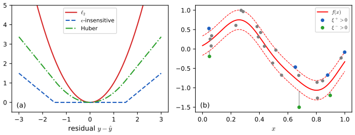
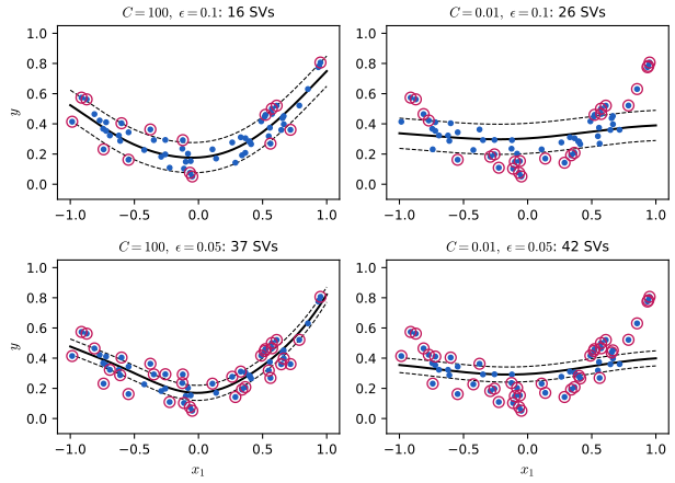
17.4 Sparse vector machines
pp. 597–598 GPs need all \(N\) training points at test time; SVMs are sparse but not probabilistic. A middle way uses the kernel only to build a feature vector, \[ \phi(\bm x)=[\kern(\bm x,\bm x_1),\dots,\kern(\bm x,\bm x_N)], \tag{17.118} \] and fits any parametric model, e.g. logistic or linear regression, on these \(N\) features. Here \(\kern\) need not be a Mercer kernel. With an \(\ell_2\) penalty (the L2VM) the weights are dense; a sparsity-promoting prior gives a sparse vector machine that keeps only a few "exemplars".
17.4.1 Relevance vector machines (RVMs)
p. 598 An \(\ell_1\) penalty (the L1VM, MAP estimation under a Laplace prior) gives sparsity but sometimes not enough. The relevance vector machine (Tipping, 2001) instead puts an independent Gaussian prior \(w_i\sim\N(0,\alpha_i^{-1})\) on each weight and estimates the precisions \(\alpha_i\) by maximising the marginal likelihood (ARD, Section 11.7.7); many \(\alpha_i\) go to infinity and their basis functions are pruned.
Filling the gap 17.23: the RVM evidence, its derivative, and the re-estimation rule \(\alpha_i=\gamma_i/\mu_i^2\) p. 598
Derivation
Model. \(\bm y=\bm\Phi\bm w+\bm\epsilon\), \(\bm\epsilon\sim\N(\bm 0,\beta^{-1}\bm I)\), \(\bm w\sim\N(\bm 0,\bm A^{-1})\), \(\bm A=\diag(\alpha_i)\). The posterior is \(\N(\bm\mu,\bm\Sigma)\) with \(\bm\Sigma=(\beta\bm\Phi^\T\bm\Phi+\bm A)^{-1}\), \(\bm\mu=\beta\bm\Sigma\bm\Phi^\T\bm y\) (Bayesian linear regression, Section 11.7), and the evidence is \(p(\bm y\given\bm\alpha,\beta)=\N(\bm y\given\bm 0,\bm C)\), \(\bm C=\beta^{-1}\bm I+\bm\Phi\bm A^{-1}\bm\Phi^\T\).
Two identities. (i) By the matrix determinant lemma, \(|\bm C|=\beta^{-N}|\bm A|^{-1}|\bm\Sigma^{-1}|\), so \(\log|\bm C|=-N\log\beta-\sum_i\log\alpha_i-\log|\bm\Sigma|\). (ii) \[ \bm y^\T\bm C^{-1}\bm y=\min_{\bm w}\{\beta\|\bm y-\bm\Phi\bm w\|^2+\bm w^\T\bm A\bm w\} \], attained at \(\bm w=\bm\mu\) (complete the square in \(\bm w\); the Woodbury identity turns the minimum value into the quadratic form). Hence \[ \log p(\bm y\given\bm\alpha,\beta)=\tfrac12\Big[N\log\beta+\sum_i\log\alpha_i+\log|\bm\Sigma|-\beta\|\bm y-\bm\Phi\bm\mu\|^2-\bm\mu^\T\bm A\bm\mu-N\log2\pi\Big]. \] Derivative. \[ \partial\log|\bm\Sigma|/\partial\alpha_i=-\partial\log|\bm\Sigma^{-1}|/\partial\alpha_i=-\tr(\bm\Sigma\,\bm e_i\bm e_i^\T)=-\Sigma_{ii} \] (gap 17.9), and by the envelope theorem the derivative of the minimum in (ii) is the partial derivative at fixed \(\bm w=\bm\mu\), namely \(\mu_i^2\). So \[ \frac{\partial\log p}{\partial\alpha_i}=\frac12\Big(\frac1{\alpha_i}-\Sigma_{ii}-\mu_i^2\Big)=0\iff\alpha_i=\frac{1-\alpha_i\Sigma_{ii}}{\mu_i^2}=\frac{\gamma_i}{\mu_i^2}, \] with \(\gamma_i=1-\alpha_i\Sigma_{ii}\in[0,1]\) measuring how well \(w_i\) is determined by the data. Similarly \(\partial/\partial\beta=0\) gives \(\beta^{-1}=\|\bm y-\bm\Phi\bm\mu\|^2/(N-\sum_i\gamma_i)\). Iterating these fixed-point equations (MacKay, 1992) and pruning when \(\alpha_i\) exceeds \(10^9\) is the algorithm in the code; at convergence the equations hold to \(10^{-4}\), and the pruned model has a higher evidence than keeping all basis functions.
Why weights are pruned, and non-convexity. As a function of one \(\alpha_i\) with the others fixed, the evidence has a finite maximiser iff \(q_i^2>s_i\) (a "quality" exceeds a "sparsity" factor), and otherwise increases monotonically to \(\alpha_i=\infty\), i.e. the weight is switched off; this analysis is carried out in full in the companion course (Bayesian and Probabilistic ML, Results 7.16–7.18). The objective is not concave in \(\log\bm\alpha\), so the RVM can stop at different local optima from different starts, which is the "not convex" entry of Table 17.1. For classification the Gaussian likelihood is replaced by the Bernoulli one and the posterior by its Laplace approximation at the mode (Result 7.20); the same \(\alpha_i=\gamma_i/\mu_i^2\) update is used. \(\square\)
17.4.2 Comparison of sparse and dense kernel methods
pp. 598–601 On a 2-D classification problem with an RBF kernel of bandwidth 0.3, the L2VM, L1VM, RVM and SVM predict about equally well, and the RVM is by far the sparsest (Figure 17.21). On 1-D regression of a noisy sinc function the predictions are again similar, and the sparsity order is RVM, then L1VM, then SVM (Figures 17.22 and 17.23).
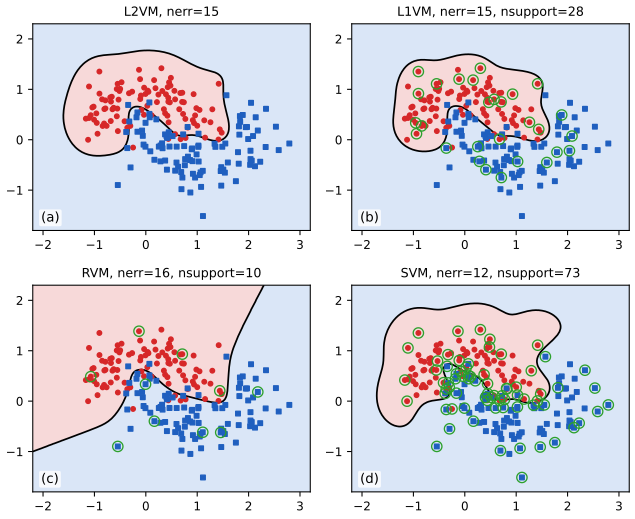
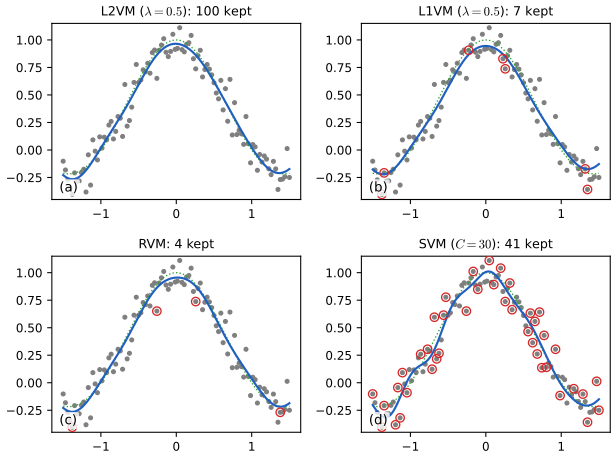
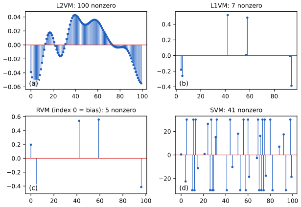
pp. 599–601 Table 17.1 compares the methods, here with the reasons behind each entry.
| Method | Optimise \(\bm w\) | Tune kernel | Sparse | Probabilistic | Multiclass | Non-Mercer \(\kern\) |
|---|---|---|---|---|---|---|
| SVM | convex QP (dual) | CV | yes (hinge zero region) | no (gap 17.19) | indirectly (OvR/OvO) | no (needs the dual) |
| L2VM | convex | EB (Gaussian prior) | no | yes | yes (softmax) | yes |
| L1VM | convex | CV | yes (\(\ell_1\)) | yes | yes | yes |
| RVM | not convex (gap 17.23) | EB | yes (ARD) | yes | yes | yes |
| GP | integrated out | EB (gap 17.9) | no | yes | yes | no (covariance) |
EB = empirical Bayes (maximise the marginal likelihood by gradients), CV = cross-validation. Methods that only use \(\phi(\bm x)\) of (17.118) as fixed features accept any similarity function; the SVM and the GP need a PSD kernel because they use it as an inner product or a covariance. Sparsity speeds up prediction but tends to make the predictive uncertainty overconfident far from the kept exemplars (the same degeneracy as in gap 17.12).
See also: Bayesian and Probabilistic ML, 7.2 relevance vector machines and the RVM demo.
17.5 Exercises
The single exercise of Chapter 17 (Murphy, 2022, pp. 601–602), restated in my own words, with a complete solution (hidden). A dagger marks the book's own flag for solutions available in its solution material; the solution here is worked independently.
Exercise 17.1 (fitting an SVM classifier by hand) †. Two points on the line: \(x_1=0\) with label \(y_1=-1\) and \(x_2=\sqrt2\) with label \(y_2=+1\), mapped to \(\R^3\) by \(\phi(x)=[1,\sqrt2x,x^2]^\T\) (the features of a second-order polynomial kernel). The maximum-margin classifier solves \(\min\|\bm w\|^2\) subject to \(y_i(\bm w^\T\phi(x_i)+w_0)\ge1\), \(i=1,2\) (17.119)–(17.121). (a) Give a vector parallel to the optimal \(\bm w\). (b) What margin does it achieve? (c) Find \(\bm w\) from margin \(=1/\|\bm w\|\). (d) Find \(w_0\). (e) Write \(f(x)=w_0+\bm w^\T\phi(x)\) explicitly as a function of \(x\).
Solution
The feature vectors are \(\phi(x_1)=(1,0,0)\) and \(\phi(x_2)=(1,2,2)\).
(a) With two points (one per class) both are support vectors, and the stationarity condition (17.73) gives \(\bm w=\alpha_1y_1\phi(x_1)+\alpha_2y_2\phi(x_2)\) with \(\alpha_1y_1+\alpha_2y_2=0\) (17.74), i.e. \(\alpha_1=\alpha_2=\alpha\) and \(\bm w=\alpha(\phi(x_2)-\phi(x_1))=\alpha(0,2,2)\). So \(\bm w\parallel(0,1,1)\): the optimal hyperplane is the perpendicular bisector of the segment joining the two feature vectors. (The first coordinate of \(\bm w\) is 0 because the constant feature cannot separate anything; its role is taken by \(w_0\).)
(b) For two points the maximum margin is half their distance: \(\|\phi(x_2)-\phi(x_1)\|=\|(0,2,2)\|=2\sqrt2\), so the margin is \(\sqrt2\).
(c) Margin \(=1/\|\bm w\|=\sqrt2\) gives \(\|\bm w\|=1/\sqrt2\). With \(\bm w=c(0,1,1)\), \(\|\bm w\|=c\sqrt2\), so \(c=\frac12\) and \(\bm w=(0,\frac12,\frac12)\) (and \(\alpha=\frac14\)).
(d) Both constraints are active: \(y_1(\bm w^\T\phi(x_1)+w_0)=-(0+w_0)=1\) gives \(w_0=-1\); check: \(y_2(\bm w^\T\phi(x_2)+w_0)=(1+1)-1=1\).
(e) \(f(x)=-1+\frac12\sqrt2\,x+\frac12x^2=\frac{x^2}2+\frac x{\sqrt2}-1\). It is \(-1\) at \(x=0\) and \(+1\) at \(x=\sqrt2\), and its positive root \(x=(\sqrt{10}-\sqrt2)/2\approx0.874\) is the decision boundary between the two points (the other root, \(-(\sqrt{10}+\sqrt2)/2\approx-2.29\), is a second boundary that the quadratic features create on the far left). The code's SMO solver with \(C=10^8\) on these two feature vectors returns \(\bm w=(0,0.5,0.5)\) and \(w_0=-1\) to seven digits. \(\square\)
Demonstrations
| Page | What it shows | In the notes |
|---|---|---|
| The marginal likelihood surface | GP regression with the SE kernel on the data of Figures 17.8 and 17.9: the log marginal likelihood over (length scale, noise), its data-fit and complexity terms, gradient ascent with the exact gradient, and the fit for any point of the map. Presets: 1 wiggly optimum; 2 smooth optimum; 3 everything is noise; 4 interpolation regime; 5 20 points. | 17.2.5, 17.2.6, gap 17.9 |
| The kernel width and the regulariser C | An RBF SVM solved live by SMO on the two-moons data and on the mixture data, with the support vectors, margins, training, test and cross-validation errors, and a clickable cross-validation map. Presets: 1–4 the four panels of Figure 17.17; 5 the mixture at its cross-validation optimum. | 17.3.3, 17.3.8, gap 17.16, gap 17.20 |
| Random Fourier features | Kernel approximation by i.i.d., orthogonal and positive random features, the Gram error against the number of features, and ridge regression on random features against exact kernel ridge regression on the noisy sinc data. Presets: 1 4 features; 2 32; 3 512; 4 orthogonal features in 16 dimensions; 5 positive features far from the origin. | 17.2.9, 17.3.9, gap 17.13 |
The Python code that produces every figure of this page is code/ch17_kernel_methods.py (see the code index). Companion demos: Gaussian process regression, GP classification, kernel functions, support vector machine, relevance vector machine, SVM path.
Notes on the book
Points where the book is imprecise or wrong
- (17.1)–(17.2), the definition. Positive entries \(\kern(\bm x_i,\bm x_j)>0\) do not make (17.1) an equality only at \(\bm c=\bm 0\) (the constant kernel is a counterexample), kernels need not be nonnegative (linear, cosine), and the linear kernel's Gram matrices are only semi-definite although the book uses it as a valid kernel. The standard (and sufficient) definition is the semi-definite one (gap 17.1).
- (17.6). \(\phi(\bm x)^\T\phi(\bm x)\) should be \(\phi(\bm x)^\T\phi(\bm x')\).
- (17.21)–(17.22). \((x_2x_2)^2\) and \((x_2x_2)(x_1x_1')\) are missing primes: \((x_2x_2')^2\), \((x_2x_2')(x_1x_1')\). The Gram matrix of the linear kernel is the \(N\times N\) inner-product matrix \(\bm X\bm X^\T\), not "the (scaled) covariance matrix of the data" (gap 17.5).
- Section 17.1.2.1, Matern smoothness. "\(k\) times differentiable iff \(\nu>k\)" is the mean-square statement (gap 17.3).
- Figure 17.9 caption and text. The two points are local maxima of the marginal likelihood, not minima (gap 17.9).
- Section 17.2.9.1. \(\bm f_X=\{f(\bm x):\bm x\in\bm Z\}\) should read \(\bm x\in\bm X\).
- Section 17.2.9.3, "the bias of the approximation decreases as we increase \(M\)". Random Fourier features are unbiased for every \(M\); their variance, \((1-k^2)^2/(2T)\), is what decreases (gap 17.13). The cost of using them is \(O(NM^2+M^3)\), not \(O(NM+M^3)\).
- (17.61), positive features. With \(\bm\omega\sim\N(\bm 0,\bm I)\) the prefactor \(e^{-\|\bm x\|^2/2}\) gives an unbiased estimate of \(e^{\bm x^\T\bm x'}\) (the softmax kernel), not of the RBF kernel; for the RBF kernel the prefactor is \(e^{-\|\bm x\|^2}\) (with bandwidth \(\sigma\): \(e^{-\|\bm x\|^2/\sigma^2}\) and \(\bm\omega\sim\N(\bm 0,\sigma^{-2}\bm I)\)). The \(\cdots,(\exp(\bm\omega_M^\T\bm x)\) also has an unmatched parenthesis.
- (17.62). \(h(\bm a)=\sqrt{1/M}[\sin\bm a,\cos\bm a]\) with \(M=2T\) features estimates \(\frac12\kern\); the normalisation of (17.59) is \(1/\sqrt T\).
- Section 17.3.2, size of the primal. The hard-margin problem (17.68) has \(D+1\) variables, not \(N+D+1\) (that count belongs to the soft-margin problem with slacks).
- After (17.80). An active constraint \(\tilde y_n(\hat{\bm w}^\T\bm x_n+\hat w_0)=1\) puts the point on the margin, not on the decision boundary (gap 17.15).
- Section 17.3.3. "replace the hard constraints that \(\tilde y_nf_n\ge0\)" should be \(\ge1\).
- (17.92). The sum runs to \(N\), not \(M\); and \(\nu\) bounds the fraction, not the number, of support vectors from below (gap 17.17).
- Section 17.3.6, "both functions are convex upper bounds on the 0-1 loss". True for the hinge loss and for the log loss in base 2; the natural-log loss \(\log(1+e^{-\eta})\) (17.99) equals \(\log2<1\) at \(\eta=0\) (gap 17.19).
- Section 17.3.8, the path. When \(C\) is large (separable data) the path ends at the hard-margin SVM, which keeps at least one support vector per class on the margin; it is not true that "no support vectors remain" (gap 17.20).
- (17.101)–(17.103). \(\sum_n\bm x_n^\T\bm x_n\) is a scalar; the matrix to invert is the Gram matrix \(\bm X\bm X^\T=[\bm x_i^\T\bm x_j]\). In (17.101) \(\tilde y_n\) should be \(y_n\) (gap 17.21).
- (17.111). Relative to (17.109), \(\frac12\|\bm w\|^2+C\sum L_\epsilon\) corresponds to \(\lambda=1/(2C)\), not \(C=1/\lambda\). The \(\epsilon\)-insensitive loss is not a variant of the Huber loss.
- (17.115). The SVR coefficients \(\alpha_n=\alpha_n^+-\alpha_n^-\) are signed (Figure 17.23d); only the two multipliers are nonnegative (gap 17.22).
References
- Murphy, K. P. (2022). Probabilistic Machine Learning: An Introduction. MIT Press, Cambridge, MA. Chapter 17, pp. 567–602. probml.github.io/pml-book/book1.html.
- Aronszajn, N. (1950). Theory of reproducing kernels. Transactions of the American Mathematical Society, 68(3), 337–404.
- Bochner, S. (1933). Monotone Funktionen, Stieltjessche Integrale und harmonische Analyse. Mathematische Annalen, 108, 378–410.
- Choromanski, K., Likhosherstov, V., Dohan, D., Song, X., Gane, A., Sarlos, T., Hawkins, P., Davis, J., Mohiuddin, A., Kaiser, L., Belanger, D., Colwell, L. and Weller, A. (2021). Rethinking attention with Performers. International Conference on Learning Representations.
- Duvenaud, D. (2014). Automatic Model Construction with Gaussian Processes. PhD thesis.
- Fan, R.-E., Chen, P.-H. and Lin, C.-J. (2005). Working set selection using second order information for training support vector machines. Journal of Machine Learning Research, 6, 1889–1918.
- Hastie, T., Rosset, S., Tibshirani, R. and Zhu, J. (2004). The entire regularization path for the support vector machine. Journal of Machine Learning Research, 5, 1391–1415.
- Hastie, T., Tibshirani, R. and Friedman, J. (2009). The Elements of Statistical Learning, 2nd edition. Springer, New York.
- Jacot, A., Gabriel, F. and Hongler, C. (2018). Neural tangent kernel: convergence and generalization in neural networks. Advances in Neural Information Processing Systems, 31.
- Kimeldorf, G. and Wahba, G. (1971). Some results on Tchebycheffian spline functions. Journal of Mathematical Analysis and Applications, 33(1), 82–95.
- MacKay, D. J. C. (1992). Bayesian interpolation. Neural Computation, 4(3), 415–447.
- Mercer, J. (1909). Functions of positive and negative type, and their connection with the theory of integral equations. Philosophical Transactions of the Royal Society A, 209, 415–446.
- Murray, I., Adams, R. P. and MacKay, D. J. C. (2010). Elliptical slice sampling. Proceedings of the Thirteenth International Conference on Artificial Intelligence and Statistics, 541–548.
- Platt, J. C. (1998). Sequential Minimal Optimization: A Fast Algorithm for Training Support Vector Machines. Technical report MSR-TR-98-14, Microsoft Research.
- Platt, J. C. (2000). Probabilistic outputs for support vector machines and comparisons to regularized likelihood methods. In Advances in Large Margin Classifiers, MIT Press, 61–74.
- Quiñonero-Candela, J. and Rasmussen, C. E. (2005). A unifying view of sparse approximate Gaussian process regression. Journal of Machine Learning Research, 6, 1939–1959.
- Rahimi, A. and Recht, B. (2007). Random features for large-scale kernel machines. Advances in Neural Information Processing Systems, 20.
- Rasmussen, C. E. and Williams, C. K. I. (2006). Gaussian Processes for Machine Learning. MIT Press, Cambridge, MA.
- Schölkopf, B., Smola, A. J., Williamson, R. C. and Bartlett, P. L. (2000). New support vector algorithms. Neural Computation, 12(5), 1207–1245.
- Schölkopf, B. and Smola, A. J. (2002). Learning with Kernels. MIT Press, Cambridge, MA.
- Stein, M. L. (1999). Interpolation of Spatial Data: Some Theory for Kriging. Springer, New York.
- Tipping, M. E. (2001). Sparse Bayesian learning and the relevance vector machine. Journal of Machine Learning Research, 1, 211–244.
- Vapnik, V., Golowich, S. E. and Smola, A. (1997). Support vector method for function approximation, regression estimation, and signal processing. Advances in Neural Information Processing Systems, 9.
- Watson, G. N. (1944). A Treatise on the Theory of Bessel Functions, 2nd edition. Cambridge University Press.
- Williams, C. K. I. (1998). Computation with infinite neural networks. Neural Computation, 10(5), 1203–1216.
- Yu, F. X., Suresh, A. T., Choromanski, K., Holtmann-Rice, D. and Kumar, S. (2016). Orthogonal random features. Advances in Neural Information Processing Systems, 29.
The numerical statements in the text (the validity of the kernels and closure rules, the Matern spectral density and its limit, the conditioning and Cholesky formulas, the marginal likelihood and its gradient against finite differences and a library, the two optima of Figure 17.9, the weight-space and function-space predictions, the inducing-point formula, the sampler on a quadrature example, the mean and variance of random features, the corrected positive features, the SMO solutions against libsvm with their KKT conditions and zero duality gap, the \(\nu\)-property, the SVR coefficients, kernel ridge regression, Platt scaling, the RVM fixed point and the answer to Exercise 17.1) were confirmed numerically.