Variational autoencoders
A variational autoencoder (VAE) is a deep latent variable model fitted by amortised stochastic variational inference: a decoder network defines the likelihood \(p_{\bm\theta}(\bm x\given\bm z)\), an encoder network outputs the approximate posterior \(q_{\bm\phi}(\bm z\given\bm x)\), and both are trained together on the evidence lower bound with the reparameterisation trick. These notes cover the basic model and its fitting algorithm, the comparison with the deterministic autoencoder, three exact rewritings of the ELBO, the \(\beta\)-VAE and InfoVAE families, multimodal, semi-supervised, sequential and missing-data VAEs, posterior collapse and its remedies, hierarchical VAEs, and vector-quantised VAEs. Beyond the book, the notes solve the linear Gaussian \(\beta\)-VAE exactly: it selects its latent directions by reverse water-filling, which shows precisely when and why posterior collapse happens.
Ch. 1 Introduction Ch. 2 Probability Ch. 3 Statistics Ch. 4 Graphical models Ch. 5 Information theory Ch. 6 Optimisation Ch. 7 Inference algorithms Ch. 8 Gaussian filtering Ch. 9 Message passing Ch. 10 Variational inference Ch. 11 Monte Carlo Ch. 12 MCMC Ch. 13 Sequential Monte Carlo Ch. 14 Predictive models Ch. 15 GLMs Ch. 16 Deep networks Ch. 17 Bayesian neural networks Ch. 18 Gaussian processes Ch. 19 Beyond iid Ch. 20 Generative models Ch. 21 VAEs Ch. 22 Autoregressive models Ch. 23 Normalizing flows Ch. 24 Energy-based models Ch. 25 Diffusion models Ch. 26 GANs Ch. 27 Discovery methods Ch. 28 Latent factor models Ch. 29 State-space models Ch. 30 Graph learning Ch. 31 Nonparametric Bayes Ch. 32 Representation learning Ch. 33 Interpretability Ch. 34 Decision making Ch. 35 Reinforcement learning Ch. 36 Causality
How to read these notes
They follow the book. Sections carry the book's numbers, and equations the book numbers keep their numbers, e.g. \((21.24)\); equations without a number are steps the book skips. Sections from the online supplement are labelled supplement and placed where the book refers to them (supplement equations are written S(21.n)).
Filling the gaps. Wherever the book writes "one can show", quotes a result from the literature, or leaves a step to the reader, an orange Filling the gap box gives the full argument. Proofs start hidden: open one with its bar, or use the buttons below. Results already proved elsewhere on the site (the ELBO identity, the reparameterisation estimator, the Gumbel-max trick, the straight-through estimator, the product of Gaussians, the MMD, the variational information bottleneck, the ignorability of missing data) are stated and linked rather than repeated.
Figures, scale and demonstrations. Every computed figure is reproduced by the Python code. Figures 21.1, 21.4 to 21.6, 21.9 to 21.14, 21.16 to 21.18 and S21.1 are diagrams and are not reproduced; Figures 21.7, 21.8 and 21.13 show samples of a text VAE-RNN, of sketch-RNN and of a 78-layer VDVAE trained on faces, which need those models and data sets and, for the last, GPU-scale training. All networks here are small and trained on the CPU: one hidden layer, 20 000 MNIST training digits, 15 to 40 epochs, in seconds to a minute each. The book's Figures 21.2, 21.3 and S21.2 use CelebA faces and convolutional models trained for 20 minutes on a GPU, so my versions are MNIST stand-ins and show the same effects less sharply; each caption says so. Five extra figures (21.x1 to 21.x5) illustrate results proved here. The ▶ Demo boxes open an interactive demonstration set to the case being discussed.
Main reference
K. P. Murphy, Probabilistic Machine Learning: Advanced Topics, MIT Press (2023; online draft of December 2025), Chapter 21, pages 791–819 (book page: probml.github.io/pml-book/book2.html), and the supplementary material, Chapter 21, pages 195–197. Section, equation, figure and algorithm numbers below refer to this book. The explanations, derivations, figures and code are my own. The book has no end-of-chapter exercises for this chapter; three practice problems are given instead.
Companion courses
The elementary VAE is introduced in Volume 1, Section 20.3.5 (and probabilistic PCA, which Section 21.3.1 below turns out to contain, in Section 20.2.2); the deep-learning course treats autoencoders and VAEs in Chapter 19. Earlier chapters of this course supply the tools: the ELBO, amortisation and the IWAE bound (gap 10.1, gap 10.3, gap 10.25), the reparameterisation trick (Section 10.2.1, gap 6.5), the Gumbel softmax and the straight-through estimator (gap 6.6, gap 6.7), the product of Gaussians (gap 2.12), the MMD (gap 2.28), rate-distortion and the information bottleneck (gap 5.20, gap 5.24) and the ignorability of missing data (gap 3.35). The generative-model overview (Section 20.3.5, latent-space interpolation) shows what VAEs are used for.
What this chapter adds: the exact form of the VAE gradient and its relation to the likelihood gradient, the correct version of Algorithm 21.1, the three decompositions of the ELBO and the split of the rate into mutual information and aggregate-posterior mismatch, why VAEs blur, the monotone effect of \(\beta\), a complete solution of the linear \(\beta\)-VAE (reverse water-filling, posterior collapse and the link to probabilistic PCA), the total-correlation split, the InfoVAE objective and the MMD in closed form, the product of experts and missing data, the M2 semi-supervised bound, why posterior collapse is a global optimum, the hierarchical ELBO, the autoregressive limit, and the VQ-VAE codebook update with its dead-code behaviour.
The chapter at a glance
- 21.2 The VAE gradient versus the likelihood gradient (gap 21.1); Algorithm 21.1 corrected (21.2); the ELBO in the augmented space and the rate split (21.3).
- 21.3 Blur and the effect of \(\beta\) (gap 21.4); the linear \(\beta\)-VAE (21.5); total correlation and the bottleneck (21.6); InfoVAE and the MMD (21.7); products of experts (21.8); missing data (21.9); the M2 bound (21.10).
- 21.4 Posterior collapse is a global optimum; free bits (gap 21.11).
- 21.5 The hierarchical ELBO and the top-down posterior (gap 21.12); autoregressive models as VAEs (21.13); the residual posterior (21.14).
- 21.6 The VQ-VAE: constant KL, straight-through, EMA codebook, dead codes (gap 21.15); the Gumbel softmax (21.16).
Notation. \(\bm x\) is the data, \(\bm z\) the latent code, \(p_{\bm\theta}(\bm x,\bm z)=p_{\bm\theta}(\bm z)p_{\bm\theta}(\bm x\given\bm z)\) the generative model with decoder \(d_{\bm\theta}\), \(q_{\bm\phi}(\bm z\given\bm x)\) the encoder, \(p_{\mathcal D}\) the data distribution, and \(\ELBO\) the evidence lower bound (the book's \(\text{Ł}\)). Densities are with respect to a reference measure, so every statement holds for discrete or continuous variables.
Prerequisites. Chapters 5, 6 and 10 of the book, and Chapter 20 of Volume 1.
21.1 Introduction
p. 791 The models of this chapter are deep latent variable models (DLVMs): a latent code \(\bm z\sim p_{\bm\theta}(\bm z)\) (21.1) is decoded by a neural network \(d_{\bm\theta}(\bm z)\) into the parameters of an exponential-family likelihood, \(\bm x\given\bm z\sim\mathrm{Expfam}(\bm x\given d_{\bm\theta}(\bm z))\) (21.2). With a Gaussian prior the model is a deep latent Gaussian model. Neither the posterior \(p_{\bm\theta}(\bm z\given\bm x)\) nor the marginal likelihood \(p_{\bm\theta}(\bm x)=\int p_{\bm\theta}(\bm x\given\bm z)p_{\bm\theta}(\bm z)\,\d\bm z\) (21.3) is available in closed form, so the model is fitted with an inference network \(q_{\bm\phi}(\bm z\given\bm x)\) trained at the same time (amortised inference, Section 10.1.5). The pair is a variational autoencoder (Kingma and Welling, 2014; Rezende, Mohamed and Wierstra, 2014): a probabilistic version of the deterministic autoencoder, in which the code is stochastic and a KL term keeps it close to the prior.
21.2 VAE basics
21.2.1 Modeling assumptions
pp. 791–792 The simplest VAE has \[ p_{\bm\theta}(\bm z,\bm x)=p_{\bm\theta}(\bm z)\,p_{\bm\theta}(\bm x\given\bm z) \tag{21.4} \] with a Gaussian prior and, for binary data, a product of Bernoullis, \[ p_{\bm\theta}(\bm x\given\bm z)=\prod_{d=1}^D\Ber\big(x_d\given\sigm(d_{\bm\theta}(\bm z))_d\big), \tag{21.5} \] together with the recognition model \[ q_{\bm\phi}(\bm z\given\bm x)=q(\bm z\given e_{\bm\phi}(\bm x))\approx p_{\bm\theta}(\bm z\given\bm x),\qquad q_{\bm\phi}(\bm z\given\bm x)=\N\big(\bm z\given\bm\mu,\diag(\exp\bm\ell)\big),\quad(\bm\mu,\bm\ell)=e_{\bm\phi}(\bm x), \tag{21.6--21.8} \] where the book writes \(\bm\ell=\log\bm\sigma\). The encoder squeezes \(\bm x\) through a stochastic bottleneck and the decoder reconstructs it (Figure 21.1, a diagram). The idea of learning a network that inverts the generative network, instead of optimising a posterior approximation per data point, goes back to the Helmholtz machine (Dayan et al., 1995), which was trained by wake-sleep (Section 10.6) and had no single objective; the VAE optimises one bound.
Two remarks on the text. First, with \(\bm\ell=\log\bm\sigma\) the covariance is \(\diag(\exp(2\bm\ell))=\diag(\bm\sigma^2)\), not \(\diag(\exp\bm\ell)\) as printed in (21.7). Second, the sentence "the VAE optimizes a variational lower bound on the log-likelihood, which means that convergence to a locally optimal MLE of the parameters is guaranteed" says more than is true; gap 21.1 shows what is and is not guaranteed.
Filling the gap 21.1: the VAE gradient is not the likelihood gradient, and the closed-form KL pp. 791–793, (21.4)–(21.8)
Proof
The bound. For each \(\bm x\), \(\log p_{\bm\theta}(\bm x)=\ELBO(\bm\theta,\bm\phi\given\bm x)+\Dkl(q_{\bm\phi}(\cdot\given\bm x)\|p_{\bm\theta}(\cdot\given\bm x))\) (gap 10.1), so the average ELBO is a lower bound on the average log-likelihood, tight exactly when the encoder returns the exact posterior at every training point.
The gradient with respect to \(\bm\theta\). Differentiating under the integral, \(\nabla_{\bm\theta}\ELBO=\E_{q_{\bm\phi}(\bm z\given\bm x)}[\nabla_{\bm\theta}\log p_{\bm\theta}(\bm x,\bm z)]\) (the entropy of \(q\) does not depend on \(\bm\theta\)). Fisher's identity gives the likelihood gradient: \(\nabla_{\bm\theta}\log p_{\bm\theta}(\bm x)=\frac{1}{p_{\bm\theta}(\bm x)}\int\nabla_{\bm\theta}p_{\bm\theta}(\bm x,\bm z)\,\d\bm z=\int p_{\bm\theta}(\bm z\given\bm x)\nabla_{\bm\theta}\log p_{\bm\theta}(\bm x,\bm z)\,\d\bm z\). The same integrand is averaged over \(q\) in the first and over the exact posterior in the second, so \[ \nabla_{\bm\theta}\ELBO=\nabla_{\bm\theta}\log p_{\bm\theta}(\bm x)-\nabla_{\bm\theta}\Dkl\big(q_{\bm\phi}\|p_{\bm\theta}(\cdot\given\bm x)\big)\Big|_{q\ \text{fixed}}, \] and a stationary point of the ELBO in \(\bm\theta\) is a stationary point of the likelihood only if the last gradient vanishes, in particular when \(q\) is the exact posterior. What stochastic gradient ascent on the ELBO can deliver, with unbiased gradients (the reparameterised estimator, gap 6.5) and suitable step sizes, is convergence to a stationary point of the ELBO in \((\bm\theta,\bm\phi)\) jointly. That is a point where the likelihood is only bounded below, and the book itself says in Section 21.2.4 that a limited posterior family makes the two objectives conflict. In the linear Gaussian case of gap 21.5 the posterior family does contain the exact posterior at the optimum, and the VAE then recovers the maximum-likelihood (probabilistic PCA) solution.
The closed-form KL. For \(q=\N(\bm\mu,\diag(\bm\sigma^2))\) and \(p=\N(\bm0,\bm I)\), using \(\E(z_k-\mu_k)^2=\sigma_k^2\) and \(\E z_k^2=\mu_k^2+\sigma_k^2\), \[ \Dkl(q\|p)=\sum_k\E_q\Big[\log\frac{q(z_k)}{p(z_k)}\Big]=\sum_k\Big[-\log\sigma_k-\tfrac12+\tfrac12(\mu_k^2+\sigma_k^2)\Big]=\frac12\sum_k\big(\mu_k^2+\sigma_k^2-1-2\log\sigma_k\big), \] which is zero iff \(\bm\mu=\bm0,\bm\sigma=\bm1\). On the trained 16-dimensional VAE of Figure 21.2 the formula gives 22.577 nats per image against 22.568 for the sample mean of \(\log q-\log p\) over 20 draws per test image. \(\square\)
21.2.2 Model fitting
p. 793 A VAE is fitted by amortised stochastic variational inference (Section 10.2.1). With a diagonal Bernoulli likelihood and a full-covariance Gaussian posterior, \(\bm z=\bm L\bm\epsilon+\bm\mu\) with \(\bm L=\bm M\odot\bm L'+\diag(\bm\sigma)\) where \(\bm M\) masks \(\bm L'\) to its strictly lower triangle, and the loss is the negative ELBO of one sample.
Algorithm 21.1: fitting a VAE with Bernoulli likelihood and full-covariance Gaussian posterior (corrected)
- Initialise \(\bm\theta,\bm\phi\).
- Repeat: sample \(\bm x\sim p_{\mathcal D}\) and \(\bm\epsilon\sim\N(\bm0,\bm I)\); compute \((\bm\mu,\log\bm\sigma,\bm L')=e_{\bm\phi}(\bm x)\); build \(\bm M=\mathrm{tril}(\bm1,-1)\) (strictly lower), \(\bm L=\bm M\odot\bm L'+\diag(\bm\sigma)\); set \(\bm z=\bm L\bm\epsilon+\bm\mu\) and \(\bm p=\sigma(d_{\bm\theta}(\bm z))\).
- \(\log q=-\sum_k(\frac12\epsilon_k^2+\frac12\log2\pi+\log\sigma_k)\); \(\log p(\bm z)=-\sum_k(\frac12z_k^2+\frac12\log2\pi)\); \(\log p(\bm x\given\bm z)=\sum_d[x_d\log p_d+(1-x_d)\log(1-p_d)]\).
- \(\mathcal L=-\log p(\bm x\given\bm z)-\log p(\bm z)+\log q\) (the negative ELBO); update \(\bm\theta\leftarrow\bm\theta-\eta\nabla_{\bm\theta}\mathcal L\), \(\bm\phi\leftarrow\bm\phi-\eta\nabla_{\bm\phi}\mathcal L\); until converged.
The book's pseudocode (based on Kingma and Welling, 2019) differs in two places, explained in gap 21.2: its mask is np.triu(np.ones(K), -1), which is not strictly lower triangular, and its loss adds the prior and entropy terms with the wrong sign.
Filling the gap 21.2: Algorithm 21.1, the density of \(\bm L\bm\epsilon+\bm\mu\), the mask and the signs p. 793, Algorithm 21.1
Proof
Density of the sample. If \(\bm\epsilon\sim\N(\bm0,\bm I)\) and \(\bm z=\bm\mu+\bm L\bm\epsilon\) with \(\bm L\) invertible, then by the change-of-variables formula \(\log q(\bm z)=\log\N(\bm\epsilon;\bm0,\bm I)-\log|\det\bm L|\), i.e. \(\bm z\sim\N(\bm\mu,\bm L\bm L^\T)\). For a triangular \(\bm L\) the determinant is the product of the diagonal, \(\det\bm L=\prod_k\sigma_k\), so \[ \log q(\bm z\given\bm x)=-\sum_k\big(\tfrac12\epsilon_k^2+\tfrac12\log2\pi+\log\sigma_k\big), \] which is line 10 of the algorithm. It needs \(\bm L\) triangular.
The mask. np.triu(np.ones(K), -1) keeps the main diagonal, everything above it and the first sub-diagonal, so \(\bm M\odot\bm L'+\diag(\bm\sigma)\) is not triangular; its determinant is not \(\prod\sigma_k\) and line 10 no longer computes \(\log q\). For \(K=4\) and a random \(\bm L'\) the printed mask gives \(\log|\det\bm L|\ne\sum_k\log\sigma_k\), while np.tril(np.ones(K), -1) gives equality to machine precision. The intended mask is the strictly lower triangle.
The signs. With the definitions on lines 10 to 12, Llogqz \(=\log q(\bm z\given\bm x)\), Llogpz \(=\log p(\bm z)\), and Llogpx \(=-\log p(\bm x\given\bm z)\) (it carries the minus sign). The negative ELBO of the sample is \(-\log p(\bm x\given\bm z)-\log p(\bm z)+\log q(\bm z\given\bm x)\) = Llogpx - Llogpz + Llogqz. Line 13 as printed, Llogpx + Llogpz - Llogqz, is \(-\log p(\bm x\given\bm z)+\log p(\bm z)-\log q\): descending it would lower the prior density of the code and the entropy of the posterior. Numerically, for one random example the printed loss is \(-4.38\) and the correct negative ELBO is \(12.14\); the corrected loss equals \(-(\log p(\bm x\given\bm z)+\log p(\bm z)-\log q)\) computed with scipy.stats.multivariate_normal to \(10^{-9}\).
The gradient. Because \(\bm z\) is a differentiable function of \((\bm\mu,\bm\sigma,\bm L',\bm\epsilon)\) with \(\bm\epsilon\) independent of \(\bm\phi\), the loss is an unbiased estimate of the negative ELBO whose \(\bm\phi\)-gradient is unbiased for the true gradient (gap 6.5, gap 10.5). \(\square\)
21.2.3 Comparison of VAEs and autoencoders
pp. 793–795 A deterministic autoencoder (AE) differs from a VAE in two ways: its objective is the reconstruction log-likelihood without a KL term, and its encoding is deterministic, \(\E[\bm z\given\bm x]\) instead of a distribution. The same code base implements both. The book fits both to CelebA with a convolutional encoder (channels 32, 64, 128, 256, 512; latent size 256), 5 epochs of batch size 256, about 20 minutes on a GPU, and compares a deterministic AE, a \(\beta\)-VAE with \(\beta=0.5\) and a VAE (Figures 21.2 and 21.3).
The main advantage of a VAE is that it is a proper generative model: decoding \(\bm z\sim\N(\bm0,\bm I)\) gives plausible images, because training pressed the encoder's codes towards the prior. An AE decodes only the codes it produced for the training set and does poorly on random inputs. Both reconstruct their inputs well; the VAE and \(\beta\)-VAE reconstructions are blurrier, for the reasons in Section 21.3.1.
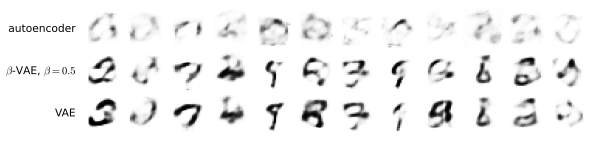
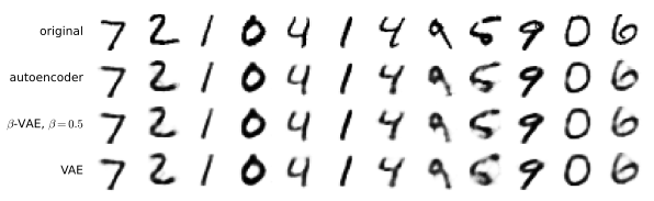
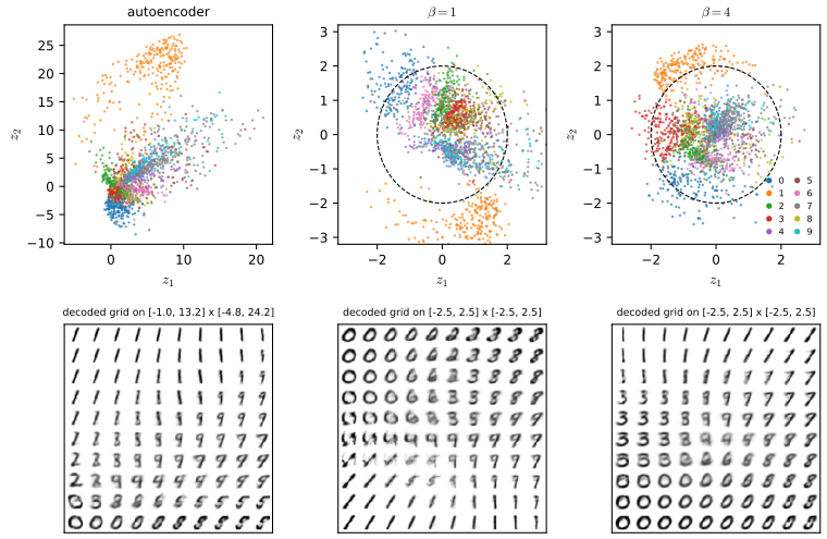
The ordering in Figure 21.3 is the rate-distortion trade-off of Section 21.3.1: more weight on the KL term means a lower rate and a higher reconstruction error. A two-dimensional latent code makes the difference between an AE and a VAE visible (Figure 21.x1): the AE places the classes wherever the reconstruction loss likes, over a range of 25 units with empty space between them, while the VAE codes are pulled into the unit-variance prior and the decoded grid changes smoothly across the plane.
See also: latent-space interpolation (Chapter 20) and VAEs in the deep-learning course.
21.2.4 VAEs optimize in an augmented space
pp. 794–796 Several equivalent forms of the ELBO explain what a VAE is optimising. Define the generative joint \(p_{\bm\theta}(\bm x,\bm z)=p_{\bm\theta}(\bm z)p_{\bm\theta}(\bm x\given\bm z)\) (21.9) with marginal \(p_{\bm\theta}(\bm x)\) (21.10) and posterior \(p_{\bm\theta}(\bm z\given\bm x)\) (21.11), and the joint inference distribution \[ q_{\mathcal D,\bm\phi}(\bm z,\bm x)=p_{\mathcal D}(\bm x)q_{\bm\phi}(\bm z\given\bm x),\qquad p_{\mathcal D}(\bm x)=\frac1N\sum_n\delta(\bm x_n-\bm x) \tag{21.12--21.13} \] with the aggregated posterior \(q_{\mathcal D,\bm\phi}(\bm z)=\int q_{\mathcal D,\bm\phi}(\bm x,\bm z)\,\d\bm x\) (21.14) and the inference likelihood \(q_{\mathcal D,\bm\phi}(\bm x\given\bm z)\) (21.15). The ELBO averaged over the data is \[ \ELBO(\bm\theta,\bm\phi\given\mathcal D)=\E_{p_{\mathcal D}}\Big[\E_{q_{\bm\phi}(\bm z\given\bm x)}[\log p_{\bm\theta}(\bm x\given\bm z)]\Big]-\E_{p_{\mathcal D}}\Dkl\big(q_{\bm\phi}(\bm z\given\bm x)\|p_{\bm\theta}(\bm z)\big) \tag{21.16} \] \[ =\E_{q_{\mathcal D,\bm\phi}}\big[\log p_{\bm\theta}(\bm x\given\bm z)+\log p_{\bm\theta}(\bm z)-\log q_{\bm\phi}(\bm z\given\bm x)\big] \tag{21.17} \] \[ =\E_{q_{\mathcal D,\bm\phi}}\Big[\log\frac{p_{\bm\theta}(\bm x,\bm z)}{q_{\mathcal D,\bm\phi}(\bm x,\bm z)}+\log p_{\mathcal D}(\bm x)\Big] \tag{21.18} \] \[ =-\Dkl\big(q_{\mathcal D,\bm\phi}(\bm x,\bm z)\|p_{\bm\theta}(\bm x,\bm z)\big)+\E_{p_{\mathcal D}}[\log p_{\mathcal D}(\bm x)] \tag{21.19} \] and, up to the additive constant \(\E_{p_{\mathcal D}}\log p_{\mathcal D}\) (written \(\overset{c}{=}\)), \[ \ELBO\overset{c}{=}-\Dkl\big(q_{\mathcal D,\bm\phi}(\bm x,\bm z)\|p_{\bm\theta}(\bm x,\bm z)\big) \tag{21.20} \] \[ \overset{c}{=}-\Dkl\big(p_{\mathcal D}(\bm x)\|p_{\bm\theta}(\bm x)\big)-\E_{p_{\mathcal D}}\Dkl\big(q_{\bm\phi}(\bm z\given\bm x)\|p_{\bm\theta}(\bm z\given\bm x)\big) \tag{21.21} \] \[ \overset{c}{=}-\Dkl\big(q_{\mathcal D,\bm\phi}(\bm z)\|p_{\bm\theta}(\bm z)\big)-\E_{q_{\mathcal D,\bm\phi}(\bm z)}\Dkl\big(q_{\mathcal D,\bm\phi}(\bm x\given\bm z)\|p_{\bm\theta}(\bm x\given\bm z)\big). \tag{21.22} \] Equation (21.21) says the ELBO is maximised by maximum likelihood (the first KL) and by fitting the true posterior (the second); with a restricted posterior family the two goals can conflict. Equation (21.22) says the VAE tries to match the aggregated posterior to the prior and, at the same time, to make the inference likelihood match the decoder. Since \(\bm x\) is usually much higher-dimensional than \(\bm z\), the second term dominates, and the VAE favours accurate reconstruction over a good posterior.
Filling the gap 21.3: the four forms of the ELBO, why the data KL is a lower bound, and the rate split pp. 794–796, (21.16)–(21.22)
Proof
Setting. Let \(p_{\mathcal D}\) have full support (a distribution on a finite set, or a density). The empirical distribution (21.13) is a sum of delta functions, for which \(\Dkl(p_{\mathcal D}\|p_{\bm\theta})\) and \(\E\log p_{\mathcal D}\) are infinite for continuous \(\bm x\); the equalities below hold as written for the population density, and for the empirical distribution of continuous data they hold with the infinite constants removed, which is what \(\overset{c}{=}\) means.
(21.16)=(21.17) is the definition of the expectation over \(q_{\mathcal D,\bm\phi}(\bm x,\bm z)=p_{\mathcal D}(\bm x)q_{\bm\phi}(\bm z\given\bm x)\), with \(\Dkl(q\|p)=\E_q[\log q-\log p]\). (21.18): write \(\log p_{\bm\theta}(\bm x\given\bm z)+\log p_{\bm\theta}(\bm z)=\log p_{\bm\theta}(\bm x,\bm z)\) and \(\log q_{\bm\phi}(\bm z\given\bm x)=\log q_{\mathcal D,\bm\phi}(\bm x,\bm z)-\log p_{\mathcal D}(\bm x)\); the \(\log p_{\mathcal D}\) terms cancel, so (21.17) equals (21.18). (21.19) follows by splitting the expectation of (21.18) into the KL and the constant.
(21.21). The chain rule of KL (the identity \(\log\frac{q(a,b)}{p(a,b)}=\log\frac{q(a)}{p(a)}+\log\frac{q(b\given a)}{p(b\given a)}\) averaged over \(q(a,b)\)) with \(a=\bm x\), \(b=\bm z\) gives \(\Dkl(q_{\mathcal D,\bm\phi}(\bm x,\bm z)\|p_{\bm\theta}(\bm x,\bm z))=\Dkl(p_{\mathcal D}\|p_{\bm\theta})+\E_{p_{\mathcal D}}\Dkl(q_{\bm\phi}(\bm z\given\bm x)\|p_{\bm\theta}(\bm z\given\bm x))\). (21.22). The same rule with \(a=\bm z\), \(b=\bm x\) gives \(\Dkl(q(\bm z)\|p(\bm z))+\E_{q(\bm z)}\Dkl(q(\bm x\given\bm z)\|p(\bm x\given\bm z))\). The book's (21.20) writes \(q_{\bm\phi}(\bm x,\bm z)\) for \(q_{\mathcal D,\bm\phi}(\bm x,\bm z)\).
Consequences. (i) Since both terms of (21.21) are non-negative, \(\Dkl(q_{\mathcal D,\bm\phi}(\bm x,\bm z)\|p_{\bm\theta}(\bm x,\bm z))\ge\Dkl(p_{\mathcal D}\|p_{\bm\theta})\), with equality iff the encoder is the exact posterior \(p_{\bm\theta}(\bm z\given\bm x)\) a.e. (Figure 21.4); this is again \(\ELBO\le\E\log p_{\bm\theta}(\bm x)\). (ii) A tiny discrete model (4 data values, 3 latent states, a random encoder) confirms that all four expressions equal each other to \(10^{-9}\).
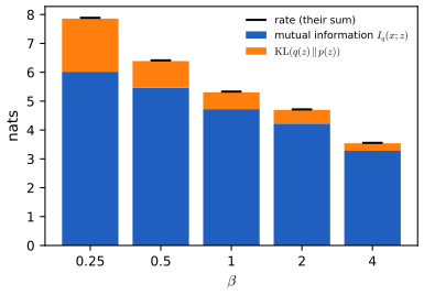
The rate split (own). The KL term of the ELBO, the rate \(R=\E_{p_{\mathcal D}}\Dkl(q_{\bm\phi}(\bm z\given\bm x)\|p(\bm z))\), splits exactly: since \(\log\frac{q(\bm z\given\bm x)}{p(\bm z)}=\log\frac{q(\bm z\given\bm x)}{q(\bm z)}+\log\frac{q(\bm z)}{p(\bm z)}\), taking \(\E_{q_{\mathcal D,\bm\phi}}\) gives \[ R=\underbrace{I_q(\bm x;\bm z)}_{\text{information about }\bm x\text{ in the code}}+\underbrace{\Dkl\big(q_{\mathcal D,\bm\phi}(\bm z)\|p(\bm z)\big)}_{\text{aggregate posterior}\ \neq\ \text{prior}}. \] Only the first part is information the code genuinely stores; the second is a mismatch that makes prior samples land where no code lives (the holes of Figure 21.x1), and it is the only part that a better prior or a better-matched posterior can remove for free. For the two-dimensional VAE with \(\beta=1\) of Figure 21.x1, \(R=5.33\) nats on test data splits into \(I_q=4.72\) and \(\Dkl(q(\bm z)\|p(\bm z))=0.58\) (Figure 21.x3); the aggregated posterior is a mixture of the 2 000 Gaussians \(q(\bm z\given\bm x_n)\), so \(\log q(\bm z)\) is exact and only the outer expectation is estimated (one draw per test digit; the sum of the two parts matches the closed-form rate to 0.03 nats). \(\square\)
21.3 VAE generalizations
21.3.1 β-VAE
pp. 797–798 VAEs tend to produce blurry images; models that optimise the exact likelihood (PixelCNNs, flows) do not. With a Gaussian decoder of fixed variance, \(\log p_{\bm\theta}(\bm x\given\bm z)=-\frac1{2\sigma^2}\|\bm x-d_{\bm\theta}(\bm z)\|_2^2+\const\) (21.23). Let \(e_{\bm\phi}(\bm x)=\E[q_{\bm\phi}(\bm z\given\bm x)]\) be the encoding and \(\mathcal X(\bm z)=\{\bm x:e_{\bm\phi}(\bm x)=\bm z\}\) the set of inputs mapped to \(\bm z\). For a fixed encoder the best decoder under squared error returns the average of the inputs in \(\mathcal X(\bm z)\), hence the blur. Better posteriors or decoders (so that distinct inputs stop sharing a code) cure it; a cheaper cure is to weaken the KL penalty, \[ \mathcal L_\beta(\bm\theta,\bm\phi\given\bm x)=\underbrace{-\E_{q_{\bm\phi}(\bm z\given\bm x)}[\log p_{\bm\theta}(\bm x\given\bm z)]}_{\mathcal L_E}+\beta\underbrace{\Dkl\big(q_{\bm\phi}(\bm z\given\bm x)\|p_{\bm\theta}(\bm z)\big)}_{\mathcal L_R}, \tag{21.24} \] the \(\beta\)-VAE (Higgins et al., 2017): \(\beta=1\) is the standard VAE and \(\beta=0\) the standard autoencoder. Varying \(\beta\) from 0 to \(\infty\) traces a rate-distortion curve (Section 5.4.2): \(\mathcal L_E\) is the distortion and \(\mathcal L_R\) the rate. With \(\beta<1\) more bits about each input are stored and reconstructions are sharper; with \(\beta>1\) the representation is more compressed.
Filling the gap 21.4: why the optimal decoder blurs, and how \(\beta\) moves the rate and the distortion pp. 797–798, (21.23)–(21.24)
Proof
The optimal decoder is the conditional mean. Fix the encoder. The decoder enters (21.16) only through \(\E_{q_{\mathcal D,\bm\phi}(\bm x,\bm z)}[\log p_{\bm\theta}(\bm x\given\bm z)]=-\frac1{2\sigma^2}\E_{q(\bm z)}\E_{q(\bm x\given\bm z)}\|\bm x-d(\bm z)\|^2+\const\), and for each \(\bm z\) with \(\bm m(\bm z)=\E_{q(\bm x\given\bm z)}[\bm x]\), \[ \E_{q(\bm x\given\bm z)}\|\bm x-\bm d\|^2=\E_{q(\bm x\given\bm z)}\|\bm x-\bm m(\bm z)\|^2+\|\bm m(\bm z)-\bm d\|^2 \] (expand around the mean; the cross term vanishes). So the unique minimiser is \(d(\bm z)=\bm m(\bm z)\) (a.e. in \(q(\bm z)\)) and the minimum is \(\tr\cov_{q(\bm x\given\bm z)}[\bm x]\), the spread of the inputs that share the code. With a deterministic encoder, \(q(\bm x\given\bm z)\) is uniform on \(\mathcal X(\bm z)\) and this is the book's statement; with a stochastic encoder \(q(\bm x\given\bm z)\propto\sum_n\delta(\bm x-\bm x_n)q_{\bm\phi}(\bm z\given\bm x_n)\), so the decoded image is the average of all training images whose posterior overlaps \(\bm z\), weighted by \(q(\bm z\given\bm x_n)\). It is sharp only if \(q(\bm x\given\bm z)\) is nearly a point mass. For the Bernoulli likelihood (21.5) the same holds: \(p\mapsto-\E[x\log p+(1-x)\log(1-p)]\) is minimised at \(p=\E[x]\) (set the derivative to zero), and for any exponential family the negative log-likelihood is a Bregman divergence in the mean parameter, minimised by the conditional mean. Both cases were confirmed by numerical minimisation on three codes with random binary inputs.
The effect of \(\beta\). Let \(D(\bm\vartheta)=\E[\mathcal L_E]\) and \(R(\bm\vartheta)=\E[\mathcal L_R]\) for parameters \(\bm\vartheta=(\bm\theta,\bm\phi)\), and let \(\bm\vartheta_i\) minimise \(D+\beta_iR\) with \(\beta_1<\beta_2\); write \(D_i,R_i\) for the values. Optimality of each gives \(D_1+\beta_1R_1\le D_2+\beta_1R_2\) and \(D_2+\beta_2R_2\le D_1+\beta_2R_1\). Adding, \((\beta_2-\beta_1)(R_2-R_1)\le0\), so \(R_2\le R_1\): a larger \(\beta\) never increases the rate. The first inequality then gives \(D_2-D_1\ge\beta_1(R_1-R_2)\ge0\): it never decreases the distortion. At an interior optimum of a smooth frontier the first-order condition is \(\d D=-\beta\,\d R\): \(\beta\) is the price, in distortion, of one nat of rate. This is the book's sentence on the rate-distortion curve made precise (and it needs only global optimality, not convexity of the achievable set).
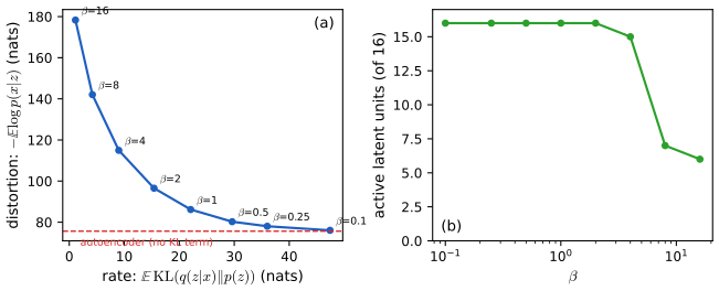
Numerically (16 latent dimensions, 20 epochs, test set of 2 000 digits; rate and distortion in nats per image, Figure 21.x2): the autoencoder has distortion 75.6; \(\beta=0.1\): rate 47.4, distortion 76.1; \(0.25\): 36.0, 78.0; \(0.5\): 29.6, 80.3; \(1\): 22.1, 86.2; \(2\): 15.4, 96.5; \(4\): 9.0, 115.0; \(8\): 4.2, 142.0; \(16\): 1.1, 178.3. Rate decreases and distortion increases at every step, as proved. \(\square\)
An exactly solvable case: the linear Gaussian β-VAE
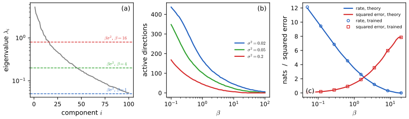
The book (footnote 5 of Section 21.4) notes that posterior collapse also occurs in linear VAEs, where the ELBO is the exact marginal likelihood. The linear model can be solved completely and shows what \(\beta\) does to each latent direction. Let the data be zero-mean Gaussian with covariance \(\bm\Sigma\) with eigenvalues \(\lambda_1\ge\dots\ge\lambda_D>0\), the decoder \(p(\bm x\given\bm z)=\N(\bm W\bm z,\sigma^2\bm I)\), the prior \(\N(\bm0,\bm I_K)\), and a Gaussian encoder with a diagonal covariance, \(q(\bm z\given\bm x)=\N(\bm A\bm x,\diag(s_1^2,\dots,s_K^2))\) as in (21.7). The \(\beta\)-VAE loss, up to constants, is \(\frac1{2\sigma^2}\E\|\bm x-\bm W\bm z\|^2+\beta\,\E\Dkl\).
Result 21.1 (reverse water-filling of the linear \(\beta\)-VAE)
For \(K\ge D\), minimising over \(\bm W,\bm A,\bm s\) gives, along the \(i\)th principal direction, \(u_i=\max\{1,\lambda_i/(\beta\sigma^2)\}\), a rate \(\frac12\log u_i\), a residual mean squared error \(\lambda_i/u_i=\min\{\lambda_i,\beta\sigma^2\}\) and a posterior variance \(1/u_i\); the minimum loss is \(\sum_i[\lambda_i/(2\sigma^2u_i)+\frac\beta2\log u_i]\). A direction with \(\lambda_i\le\beta\sigma^2\) is collapsed (posterior equal to the prior, rate 0). For \(K<D\) only the \(K\) largest directions can be used.
Filling the gap 21.5: proof of Result 21.1, the link to probabilistic PCA, and posterior collapse in the linear VAE pp. 797–798 and footnote 5, p. 807
Proof
Step 1, the decoder. Fix \((\bm A,\bm S)\), \(\bm S=\diag(\bm s^2)\). Then \(\bm z=\bm A\bm x+\bm S^{1/2}\bm\varepsilon\) and \((\bm x,\bm z)\) are jointly Gaussian. Minimising \(\E\|\bm x-\bm W\bm z\|^2\) over \(\bm W\) is least squares: \(\bm W^*=\E[\bm x\bm z^\T]\E[\bm z\bm z^\T]^{-1}=\bm\Sigma\bm A^\T(\bm A\bm\Sigma\bm A^\T+\bm S)^{-1}\) and the minimum is the posterior covariance of \(\bm x\) given \(\bm z\), by the Woodbury identity \[ \mathfrak D^*=\Tr\big(\bm\Sigma-\bm\Sigma\bm A^\T(\bm A\bm\Sigma\bm A^\T+\bm S)^{-1}\bm A\bm\Sigma\big)=\Tr\big((\bm\Sigma^{-1}+\bm B)^{-1}\big),\qquad\bm B=\bm A^\T\bm S^{-1}\bm A. \] Step 2, the rate. Averaging the Gaussian KL over \(\bm x\), \(\mathfrak R=\frac12\sum_k[(\bm A\bm\Sigma\bm A^\T)_{kk}+s_k^2-1-\log s_k^2]\). Let \(\tilde{\bm A}=\bm S^{-1/2}\bm A\) (rows \(\tilde{\bm a}_k^\T\)), so \(\bm B=\tilde{\bm A}^\T\tilde{\bm A}\), and \(c_k=\tilde{\bm a}_k^\T\bm\Sigma\tilde{\bm a}_k\), so \((\bm A\bm\Sigma\bm A^\T)_{kk}=s_k^2c_k\). With \(t=s_k^2(1+c_k)\) each summand is \(t-1-\log t+\log(1+c_k)\ge\log(1+c_k)\), because \(t-1-\log t\ge0\) with equality iff \(t=1\). Hence \(\mathfrak R\ge\frac12\sum_k\log(1+c_k)\), with equality iff \(s_k^2=1/(1+c_k)\). Note that \(\mathfrak D^*\) depends on \((\bm A,\bm S)\) only through \(\bm B\).
Step 3, Hadamard. The matrix \(\bm I_K+\tilde{\bm A}\bm\Sigma\tilde{\bm A}^\T\) is positive semi-definite with diagonal entries \(1+c_k\), so Hadamard's inequality gives \(\prod_k(1+c_k)\ge\det(\bm I_K+\tilde{\bm A}\bm\Sigma\tilde{\bm A}^\T)=\det(\bm I_D+\bm\Sigma^{1/2}\bm B\bm\Sigma^{1/2})=\det(\bm I+\bm C)\), by Sylvester's determinant identity, with \(\bm C=\bm\Sigma^{1/2}\bm B\bm\Sigma^{1/2}\succeq0\) of rank at most \(K\), with equality iff \(\tilde{\bm A}\bm\Sigma\tilde{\bm A}^\T\) is diagonal. Since \((\bm\Sigma^{-1}+\bm B)^{-1}=\bm\Sigma^{1/2}(\bm I+\bm C)^{-1}\bm\Sigma^{1/2}\), \[ \mathcal L\ \ge\ g(\bm C)=\frac1{2\sigma^2}\Tr\big(\bm\Sigma(\bm I+\bm C)^{-1}\big)+\frac\beta2\log\det(\bm I+\bm C). \] Step 4, von Neumann. For positive semi-definite \(\bm P,\bm Q\), \(\Tr(\bm P\bm Q)\ge\sum_i\lambda_i^{\downarrow}(\bm P)\lambda_i^{\uparrow}(\bm Q)\) (the trace is smallest when the largest eigenvalues of one are paired with the smallest of the other; von Neumann's trace inequality). Let \(\gamma_1\ge\dots\ge\gamma_D\ge0\) be the eigenvalues of \(\bm C\); then \((\bm I+\bm C)^{-1}\) has eigenvalues \(1/(1+\gamma_i)\) in ascending order, so \(g(\bm C)\ge\sum_i f_i(1+\gamma_i)\) with \(f_i(u)=\frac{\lambda_i}{2\sigma^2u}+\frac\beta2\log u\), and at most \(K\) of the \(\gamma_i\) are non-zero.
Step 5, the scalar problems. \(f_i'(u)=\frac1{2u}(\beta-\frac{\lambda_i}{\sigma^2u})\) is negative for \(u<\lambda_i/(\beta\sigma^2)\) and positive beyond, so over \(u\ge1\) the minimiser is \(u_i=\max\{1,\lambda_i/(\beta\sigma^2)\}\); this is non-increasing in \(i\), consistent with the ordering of the \(\gamma_i\). The lower bound is \(\sum_if_i(u_i)\) (with the constraint \(\gamma_i=0\) for \(i>K\) when \(K<D\)).
Step 6, attainment. Let \(\bm U\) hold the eigenvectors and put \(\bm A=\bm S^{1/2}\diag(\sqrt{(u_i-1)/\lambda_i})\bm U^\T\) with \(s_i^2=1/u_i\) (rows for \(i\le K\); unused units have \(\bm A\)-row 0 and \(s=1\), i.e. they equal the prior). Then \(c_i=u_i-1\), \(\tilde{\bm A}\bm\Sigma\tilde{\bm A}^\T=\diag(u_i-1)\) is diagonal (Hadamard equality), \(s_i^2=1/(1+c_i)\) (Step 2 equality), and \(\bm B\) shares eigenvectors with \(\bm\Sigma\) (von Neumann equality). By Step 1 the decoder is \(\bm w_i=\sqrt{\lambda_i(u_i-1)/u_i}\,\bm U_{\cdot i}\). \(\square\)
Consequences. (1) Reverse water-filling. Each direction costs \(\frac12\log(\lambda_i/(\beta\sigma^2))\) nats and leaves error exactly \(\beta\sigma^2\); the "water level" \(\beta\sigma^2\) caps the error, as in Gaussian rate-distortion theory (gap 5.20). (2) Posterior collapse. Direction \(i\) is unused iff \(\lambda_i\le\beta\sigma^2\): its posterior equals the prior, KL is exactly 0, and this is a global optimum, not a failed optimisation. Raising \(\beta\) or \(\sigma^2\) lifts the water over the spectrum and switches directions off from the weakest up. (3) Probabilistic PCA. At \(\beta=1\), \(\bm W\bm W^\T=\bm U(\bm\Lambda-\sigma^2\bm I)_+\bm U^\T\), the maximum-likelihood solution of probabilistic PCA with noise \(\sigma^2\) (Volume 1, Section 20.2.2): the VAE with a linear decoder recovers it, and the diagonal posterior is what aligns the code with the principal axes. (4) The rate-distortion slope. Summing over directions, the total error \(D(\beta)\) and rate \(R(\beta)\) satisfy \(\d D/\d R=-2\sigma^2\beta\) (the factor \(2\sigma^2\) because \(D\) is a squared error and the loss uses \(D/(2\sigma^2)\)), the first-order condition of gap 21.4. (5) Numbers. For eigenvalues \((4,2,1,0.5,0.25,0.1)\), \(\sigma^2=0.25\) and \(\beta=1\): four directions are used, the last two (\(\lambda\le\sigma^2\)) are collapsed, the rate is 3.466 nats, the error 1.350 and the loss 6.166. The exact expected loss was minimised by Adam on data rotated by a random orthogonal matrix (so the optimiser has to find the eigenbasis): for \(\beta=0.3,1,3\) the trained loss, rate and error agree with the formulas to three decimals (e.g. \(\beta=1\): 6.1657 against 6.1657), the decoder's \(\bm W\bm W^\T\) has eigenvalues \((3.75,1.75,0.75,0.25,0,0)=(\lambda-\sigma^2)_+\), and 3 000 random encoders never beat the water-filling loss. \(\blacksquare\)
21.3.1.1 Disentangled representations
p. 798 A representation is "disentangled" if each latent coordinate captures a different factor of variation, formalised by the total correlation (the multi-information) \[ \mathrm{TC}(\bm z)=\sum_k\Hent(z_k)-\Hent(\bm z)=\Dkl\Big(p(\bm z)\Big\|\prod_kp_k(z_k)\Big), \tag{21.25} \] zero iff the components are independent. Achille and Soatto (2018) prove that \(\beta>1\) decreases it. Locatello et al. (2019; the book's [Loc+18]) prove that nonlinear latent-variable models are unidentifiable: for any disentangled representation there is an equivalent fully entangled one with exactly the same likelihood, so tuning \(\beta\) cannot by itself recover the true factors; an inductive bias in the encoder, decoder, prior, data or algorithm is needed (Section 32.4.1).
21.3.1.2 Connection with information bottleneck
pp. 798–799 The \(\beta\)-VAE is an unsupervised information bottleneck (Section 5.6). With input \(\bm x\), bottleneck \(\bm z\) and target \(\tilde{\bm x}\) the unsupervised IB objective is \(\mathcal L_{\mathrm{UIB}}=\beta I(\bm z;\bm x)-I(\bm z;\tilde{\bm x})\) (21.26)–(21.27), with \(p(\bm x,\bm z)=p_{\mathcal D}(\bm x)p(\bm z\given\bm x)\) (21.28) and \(p(\bm z,\tilde{\bm x})=\int p_{\mathcal D}(\bm x)p(\bm z\given\bm x)p(\tilde{\bm x}\given\bm z)\,\d\bm x\) (21.29): predict \(\tilde{\bm x}\) from \(\bm z\) while memorising as little as possible of \(\bm x\). Its variational upper bound (5.181) is \[ \mathcal L_{\mathrm{UVIB}}=-\E_{q_{\mathcal D,\bm\phi}(\bm z,\bm x)}[\log p_{\bm\theta}(\bm x\given\bm z)]+\beta\,\E_{p_{\mathcal D}}\Dkl\big(q_{\bm\phi}(\bm z\given\bm x)\|p_{\bm\theta}(\bm z)\big), \tag{21.30} \] which is the \(\beta\)-VAE objective (21.24) averaged over the data.
Filling the gap 21.6: the three-way split of the rate, the bound (21.30), and what unidentifiability means pp. 798–799, (21.25)–(21.30)
Proof
Total correlation. \(\sum_k\Hent(z_k)-\Hent(\bm z)=\E[\log p(\bm z)-\sum_k\log p_k(z_k)]=\Dkl(p\|\prod_kp_k)\ge0\), zero iff \(p=\prod_kp_k\) (Volume 1, Result 6.2).
Where the total correlation sits in the ELBO (own). For a factorised prior \(p(\bm z)=\prod_kp_k(z_k)\) and the aggregated posterior \(q(\bm z)\) with marginals \(q_k\), adding and subtracting \(\log\prod_kq_k(z_k)\) in \(\log\frac{q(\bm z)}{p(\bm z)}\) gives \(\Dkl(q(\bm z)\|p(\bm z))=\mathrm{TC}(q)+\sum_k\Dkl(q_k\|p_k)\). With gap 21.3, \[ \E_{p_{\mathcal D}}\Dkl(q(\bm z\given\bm x)\|p(\bm z))=I_q(\bm x;\bm z)+\mathrm{TC}(q)+\sum_k\Dkl(q_k\|p_k). \] A larger \(\beta\) weights all three terms. The identity does not by itself say that \(\beta>1\) lowers the TC more than the other two (the cited result is a statement about trained representations); methods such as the \(\beta\)-TCVAE therefore penalise the TC term alone. A toy check: for a \(2\times2\) joint distribution and a factorised reference, the split holds to \(10^{-9}\).
The bound (21.30). (i) \(I(\bm z;\bm x)=\E_{p_{\mathcal D}}\Dkl(q(\bm z\given\bm x)\|q(\bm z))\le\E_{p_{\mathcal D}}\Dkl(q(\bm z\given\bm x)\|p(\bm z))\) for every \(p(\bm z)\), the gap being \(\Dkl(q(\bm z)\|p(\bm z))\ge0\) (gap 21.3). (ii) With \(\tilde{\bm x}=\bm x\), \(I(\bm z;\bm x)=\Hent(\bm x)-\Hent(\bm x\given\bm z)\) and \(\Hent(\bm x\given\bm z)=-\E\log q(\bm x\given\bm z)\le-\E\log p_{\bm\theta}(\bm x\given\bm z)\) (cross-entropy exceeds entropy), so \(-I(\bm z;\bm x)\le-\Hent(\bm x)-\E\log p_{\bm\theta}(\bm x\given\bm z)\). Combining, \(\beta I(\bm z;\bm x)-I(\bm z;\bm x)\) is bounded above by \(\mathcal L_{\mathrm{UVIB}}-\Hent(\bm x)\); the constant \(\Hent(\bm x)\) does not depend on the parameters. The full variational IB bounds, with their slacks, are in gap 5.24.
Unidentifiability, the linear-Gaussian case. If the posterior covariance is isotropic and the prior is \(\N(\bm0,\bm I)\), the ELBO is unchanged by replacing \(\bm z\) with \(\bm R\bm z\) for any orthogonal \(\bm R\) (encoder \(\bm R\bm A\), decoder \(\bm W\bm R^\T\)): the KL and the likelihood are invariant. The rotated code has independent components too, yet each now mixes all the factors, so the objective cannot tell a disentangled solution from an entangled one. A diagonal, non-isotropic posterior breaks this symmetry in the linear model, which is why gap 21.5 finds the principal axes. In the nonlinear case Locatello et al. (2019) show that the symmetry group is much larger. \(\square\)
21.3.2 InfoVAE
pp. 799–800 The standard ELBO has two drawbacks (Section 21.2.4): it ignores the latent code when the decoder is powerful (Section 21.4), and the KL terms in data space and latent space are mismatched. The InfoVAE objective (Zhao, Song and Ermon, 2019) generalises it: \[ \ELBO(\bm\theta,\bm\phi\given\bm x)=-\lambda\,\Dkl\big(q_{\bm\phi}(\bm z)\|p_{\bm\theta}(\bm z)\big)-\E_{q_{\bm\phi}(\bm z)}\Dkl\big(q_{\bm\phi}(\bm x\given\bm z)\|p_{\bm\theta}(\bm x\given\bm z)\big)+\alpha\,I_q(\bm x;\bm z), \tag{21.31} \] with \(\alpha\ge0\) weighting the mutual information and \(\lambda\ge0\) trading the latent-space against the data-space KL; \(\alpha=0,\lambda=1\) is (21.22). Because \(I_q\) is intractable (21.32), use \(q(\bm x\given\bm z)=p_{\mathcal D}(\bm x)q(\bm z\given\bm x)/q(\bm z)\) to rewrite it as \[ \ELBO=\E_{q_{\bm\phi}(\bm x,\bm z)}\Big[\log p_{\bm\theta}(\bm x\given\bm z)-\log\frac{q_{\bm\phi}(\bm z)^{\lambda+\alpha-1}p_{\mathcal D}(\bm x)}{p_{\bm\theta}(\bm z)^\lambda q_{\bm\phi}(\bm z\given\bm x)^{\alpha-1}}\Big] \tag{21.33--21.34} \] \[ =\E_{p_{\mathcal D}}\E_{q_{\bm\phi}(\bm z\given\bm x)}[\log p_{\bm\theta}(\bm x\given\bm z)]-(1-\alpha)\E_{p_{\mathcal D}}\Dkl\big(q_{\bm\phi}(\bm z\given\bm x)\|p_{\bm\theta}(\bm z)\big)-(\alpha+\lambda-1)\Dkl\big(q_{\bm\phi}(\bm z)\|p_{\bm\theta}(\bm z)\big)-\E_{p_{\mathcal D}}\log p_{\mathcal D}(\bm x). \tag{21.35} \] The first two terms are optimised by reparameterisation. The last KL involves the aggregated posterior \(q_{\bm\phi}(\bm z)\), which is intractable but easy to sample (draw \(\bm x\sim p_{\mathcal D}\), then \(\bm z\sim q_{\bm\phi}(\bm z\given\bm x)\)): an implicit distribution, as in a GAN, so one may replace the KL by any strict divergence, and this does not affect the optimum. Theorem 1 (Zhao et al., 2019, Proposition 2): for continuous \(\mathcal X,\mathcal Z\), \(\alpha<1\) and \(\lambda>0\), and any fixed value of \(I_q(\bm x;\bm z)\), the approximate InfoVAE loss with any strict divergence \(D(q_{\bm\phi}(\bm z),p_{\bm\theta}(\bm z))\) is globally optimised if \(p_{\bm\theta}(\bm x)=p_{\mathcal D}(\bm x)\) and \(q_{\bm\phi}(\bm z\given\bm x)=p_{\bm\theta}(\bm z\given\bm x)\).
21.3.2.1 Connection with MMD VAE
p. 800 For \(\alpha=1\) the objective is \(\ELBO\overset{c}{=}\E_{p_{\mathcal D}}\E_{q(\bm z\given\bm x)}[\log p(\bm x\given\bm z)]-\lambda\Dkl(q(\bm z)\|p(\bm z))\) (21.36). The MMD VAE replaces the KL by the squared maximum mean discrepancy (Section 2.7.3); with \(\lambda=1\) and the sign swapped, \(\mathcal L=\E_{p_{\mathcal D}}\E_{q(\bm z\given\bm x)}[-\log p(\bm x\given\bm z)]+\mathrm{MMD}(q_{\bm\phi}(\bm z),p(\bm z))\) (21.37), with \[ \mathrm{MMD}(p,q)=\E_{p(\bm z),p(\bm z')}K(\bm z,\bm z')+\E_{q(\bm z),q(\bm z')}K(\bm z,\bm z')-2\E_{p(\bm z),q(\bm z')}K(\bm z,\bm z') \tag{21.38} \] and \(K\) an RBF kernel \(e^{-\|\bm z-\bm z'\|^2/(2\sigma^2)}\). In practice the posterior means \(\bm z_n=e_{\bm\phi}(\bm x_n)\) of a minibatch are compared with as many draws from \(\mathcal N(\bm0,\bm I)\). With a Gaussian decoder of fixed variance the negative log-likelihood is \(\|\bm x-d_{\bm\theta}(\bm z)\|^2\) (21.39) and the whole model is deterministic. 21.3.2.2 \(\beta\)-VAEs. With \(\alpha=0,\lambda=1\) one gets back the ELBO; for free \(\lambda>0\) and \(\alpha=1-\lambda\) one gets the \(\beta\)-VAE with \(\beta=\lambda\). 21.3.2.3 Adversarial autoencoders. With \(\alpha=\lambda=1\) and \(D\) the Jensen–Shannon divergence (minimised by training a binary discriminator, Section 26.2.2 of the book) one gets the adversarial autoencoder (Makhzani et al., 2015).
Filling the gap 21.7: the InfoVAE rewriting, its special cases, Theorem 1, and the MMD in closed form pp. 799–800, (21.31)–(21.39)
Proof
(21.33)–(21.35). All expectations are under \(q_{\bm\phi}(\bm x,\bm z)=p_{\mathcal D}(\bm x)q_{\bm\phi}(\bm z\given\bm x)\). Write the three terms of (21.31) as expectations of log-ratios: \(-\lambda\log\frac{q(\bm z)}{p(\bm z)}-\log\frac{q(\bm x\given\bm z)}{p(\bm x\given\bm z)}-\alpha\log\frac{q(\bm z)}{q(\bm z\given\bm x)}\) (the mutual information is \(\E\log\frac{q(\bm z\given\bm x)}{q(\bm z)}\), (21.32)). Insert \(\log q(\bm x\given\bm z)=\log p_{\mathcal D}(\bm x)+\log q(\bm z\given\bm x)-\log q(\bm z)\). The terms are then \[ \log p(\bm x\given\bm z)-\log p_{\mathcal D}(\bm x)+\lambda\log p(\bm z)-(\lambda+\alpha-1)\log q(\bm z)+(\alpha-1)\log q(\bm z\given\bm x), \] which is (21.34). Using \(\lambda=(1-\alpha)+(\alpha+\lambda-1)\), regroup the three \(\log\)-density terms as \(-(1-\alpha)[\log q(\bm z\given\bm x)-\log p(\bm z)]-(\alpha+\lambda-1)[\log q(\bm z)-\log p(\bm z)]\); the expectation of the first bracket is the rate and of the second \(\Dkl(q(\bm z)\|p(\bm z))\): this is (21.35). On a small discrete model with random encoder and decoder, (21.31) and (21.35) agree to \(10^{-9}\) for five choices of \((\alpha,\lambda)\).
Special cases. \(\alpha=0,\lambda=1\): the coefficients are \((1,0)\) and (21.35) is the averaged ELBO of (21.16) minus \(\E\log p_{\mathcal D}\) (the constant). \(\alpha=1-\lambda\): the coefficients are \((\lambda,0)\): \(\E\log p(\bm x\given\bm z)-\lambda\cdot\mathrm{rate}\), the \(\beta\)-VAE with \(\beta=\lambda\). \(\alpha=1\): the coefficients are \((0,\lambda)\), which is (21.36). (21.35) needs \(1-\alpha\ge0\) for the second term to be a penalty, which is why the theorem requires \(\alpha<1\).
Theorem 1. Fix \(I_q(\bm x;\bm z)\), so the third term of (21.31) is fixed. The remaining two terms are \(-\lambda D(q(\bm z),p(\bm z))\le0\) and \(-\E_{q(\bm z)}\Dkl(q(\bm x\given\bm z)\|p(\bm x\given\bm z))\le0\) (for \(D\) a strict divergence), both zero iff \(q(\bm z)=p(\bm z)\) and \(q(\bm x\given\bm z)=p(\bm x\given\bm z)\) a.e. Together these say \(q_{\mathcal D,\bm\phi}(\bm x,\bm z)=p_{\bm\theta}(\bm x,\bm z)\); marginalising over \(\bm z\) gives \(p_{\mathcal D}=p_{\bm\theta}\) and dividing by it gives \(q_{\bm\phi}(\bm z\given\bm x)=p_{\bm\theta}(\bm z\given\bm x)\). Conversely, those two conditions make both terms vanish, so the loss attains its maximum over all models with that value of \(I_q\). (If the model class cannot reach the condition at the prescribed \(I_q\), the statement is about the unconstrained maximum; the theorem is a statement about what the objective rewards, not about what a given network class attains.)
The MMD in closed form for Gaussians (own). Let \(K(\bm z,\bm z')=e^{-\|\bm z-\bm z'\|^2/(2s^2)}\), \(\bm z\sim\N(\bm m_1,\bm\Sigma_1)\), \(\bm z'\sim\N(\bm m_2,\bm\Sigma_2)\) independent. Then \(\bm u=\bm z-\bm z'\sim\N(\bm m_1-\bm m_2,\bm\Sigma_1+\bm\Sigma_2)\) and \(K=(2\pi s^2)^{d/2}\N(\bm u;\bm0,s^2\bm I)\), so \[ \E K=(2\pi s^2)^{d/2}\int\N(\bm u;\bm0,s^2\bm I)\N(\bm u;\bm m_1-\bm m_2,\bm\Sigma_1+\bm\Sigma_2)\,\d\bm u=\det\!\big(\bm I+(\bm\Sigma_1+\bm\Sigma_2)/s^2\big)^{-1/2}\exp\!\Big(-\tfrac12(\bm m_1-\bm m_2)^\T(s^2\bm I+\bm\Sigma_1+\bm\Sigma_2)^{-1}(\bm m_1-\bm m_2)\Big), \] using \(\int\N(\bm u;\bm a,\bm A)\N(\bm u;\bm b,\bm B)\,\d\bm u=\N(\bm a;\bm b,\bm A+\bm B)\). For \(\N(0,1)\) against \(\N(\delta,1)\) with \(s=1\) in one dimension, \(\E K_{pp}=\E K_{qq}=1/\sqrt3\) and \(\E K_{pq}=e^{-\delta^2/6}/\sqrt3\), so \(\mathrm{MMD}^2=\frac2{\sqrt3}(1-e^{-\delta^2/6})\) (see practice problem 21.3). For \(\delta=1.3\) this is 0.2835; the estimator (21.38) with 3 000 draws from each gives 0.278. The MMD vanishes iff \(p=q\) for a characteristic kernel such as the RBF kernel, and its estimators are discussed in gap 2.28. \(\square\)
21.3.3 Multimodal VAEs
pp. 800–802 To model several kinds of data (images, text, ...) jointly, assume \(M\) modalities conditionally independent given one code, \[ p_{\bm\theta}(\bm x_1,\dots,\bm x_M,\bm z)=p(\bm z)\prod_{m=1}^Mp_{\bm\theta}(\bm x_m\given\bm z), \tag{21.40} \] with ELBO \(\E_{q(\bm z\given\bm X)}[\sum_m\log p(\bm x_m\given\bm z)]-\Dkl(q(\bm z\given\bm X)\|p(\bm z))\) (21.41). Weights \(\lambda_m\ge0\) rescale the likelihoods and \(\beta\ge0\) the KL (21.42); an indicator \(O_m\) marks the observed modalities, so only \(\sum_{m:O_m=1}\lambda_m\log p(\bm x_m\given\bm z)\) appears (21.43). The difficulty is computing \(q(\bm z\given\bm X)\) for any subset of modalities. The exact posterior is \[ p(\bm z\given\bm X)=\frac{p(\bm z)}{p(\bm X)}\prod_mp(\bm x_m\given\bm z)\propto p(\bm z)\prod_m\frac{p(\bm z\given\bm x_m)}{p(\bm z)}\approx p(\bm z)\prod_m\tilde q(\bm z\given\bm x_m) \tag{21.44--21.46} \] a product of experts (Section 24.1.1) with one learned expert \(\tilde q(\bm z\given\bm x_m)\) per modality and the prior as an extra expert; any subset is handled by dropping the missing factors. For Gaussians, \(\prod_{m=0}^M\N(\bm z\given\bm\mu_m,\bm\Lambda_m^{-1})\propto\N(\bm z\given\bm\mu,\bm\Sigma)\) with \[ \bm\Sigma=\Big(\sum_m\bm\Lambda_m\Big)^{-1},\qquad\bm\mu=\bm\Sigma\sum_m\bm\Lambda_m\bm\mu_m \tag{21.47} \] (Equation (2.154)): precisions add and the mean is the precision-weighted average (Figure 21.5, a diagram). For a linear Gaussian (factor-analysis) model with \(\tilde q(\bm z\given\bm x_m)=p(\bm z\given\bm x_m)\) form this is exactly the posterior (Wu and Goodman, 2018); in general it is an approximation. The individual experts must be trained as well as the joint model; Vedantam et al. (2018) use a "triple ELBO", and Wu and Goodman (2018) the simpler sum of the ELBO for all modalities, each single modality and \(J\) random subsets, \[ \ELBO(\bm\theta,\bm\phi\given\bm X)=\ELBO(\bm x_1,\dots,\bm x_M)+\sum_{m=1}^M\ELBO(\bm x_m)+\sum_{j\in\mathcal J}\ELBO(\bm X_j), \tag{21.48} \] which extends to the semi-supervised case with few aligned pairs. This handles a fixed set of missingness patterns; arbitrary patterns are treated in the supplement (next).
Filling the gap 21.8: the product of experts is the exact posterior in the linear Gaussian case, and dropping a modality is exact pp. 801–802, (21.44)–(21.47)
Proof
(21.44)–(21.46). Conditional independence gives \(p(\bm x_1,\dots,\bm x_M\given\bm z)=\prod_mp(\bm x_m\given\bm z)\) and Bayes' rule \(p(\bm x_m\given\bm z)=p(\bm z\given\bm x_m)p(\bm x_m)/p(\bm z)\); the \(p(\bm x_m)\) do not depend on \(\bm z\). If only a subset \(\mathcal O\) of the modalities is observed, \(p(\bm z\given\bm X_{\mathcal O})\propto p(\bm z)\prod_{m\in\mathcal O}p(\bm x_m\given\bm z)\): the unobserved modalities are integrated out, \(\int p(\bm x_m\given\bm z)\,\d\bm x_m=1\), so their factors are simply absent. That is the sense in which dropping a modality is exact and needs no new inference network.
The Gaussian product (21.47). Multiplying Gaussian densities adds the quadratic forms in the exponent: precisions add and the linear terms \(\bm\Lambda_m\bm\mu_m\) add (gap 2.12); this is a statement about the product of densities, which is normalised afterwards. A numerical experiment on random 2-d experts confirms that the product of the densities is proportional to \(\N(\bm\mu,\bm\Sigma)\) with constant log-ratio to \(10^{-10}\).
Exactness for a linear Gaussian model. Let \(p(\bm z)=\N(\bm0,\bm I)\), \(p(\bm x_m\given\bm z)=\N(\bm W_m\bm z,\sigma_m^2\bm I)\). Then \(p(\bm x_m\given\bm z)\) is, as a function of \(\bm z\), an unnormalised Gaussian with precision \(\bm\Lambda_m=\bm W_m^\T\bm W_m/\sigma_m^2\) and \(\bm\Lambda_m\bm\mu_m=\bm W_m^\T\bm x_m/\sigma_m^2\), which is exactly the ratio expert \(p(\bm z\given\bm x_m)/p(\bm z)\) (its precision is the single-modality posterior precision minus the prior precision, \(\bm\Lambda_m=\bm P_m-\bm I\)). The product (21.47) of the prior and these experts is then the joint posterior. The expert may be singular (if \(\dim\bm x_m<K\)), which is why one adds precisions in information form instead of inverting each. Numerically, with \(K=3\) and two modalities of dimensions 4 and 5, the PoE mean and precision equal the exact joint posterior to machine precision, and dropping one modality reproduces the single-modality posterior exactly. In a trained MVAE the experts are not constrained to be ratios and the PoE is an approximation; it is also a poor model if the experts are overconfident. \(\square\)
S21.0.1 VAEs with missing data supplement
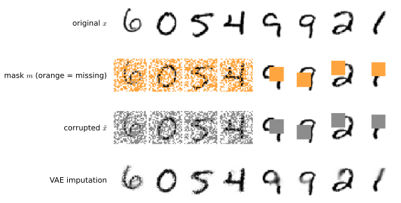
Supplement pp. 195–197 Parts of the data vector may be unknown. Let \(\bm m\in\{0,1\}^D\) with \(m_j=1\) if \(x_j\) is missing, and split \(\bm X\) into the observed \(\bm X_o\) and hidden \(\bm X_h\). The mechanism is MCAR if \(p(\bm M\given\bm X_o,\bm X_h)=p(\bm M)\), MAR if it equals \(p(\bm M\given\bm X_o)\), and NMAR otherwise. In the first two cases the mechanism can be ignored; for NMAR it must be modelled, because the absence of a value is informative (Little and Rubin, 1987). For VAEs, MCAR is modelled by treating the missing values as latent variables: since missing leaf nodes of a directed model do not affect their parents, they are ignored when computing \(p(\bm z\given\bm x_o)\). The trouble is the amortised encoder, which is trained on complete inputs; the product-of-experts solution handles missing blocks (modalities) but not arbitrary patterns such as occluded pixels, and does not handle NMAR. Collier, Nazabal and Williams (2020) include the indicators in the model (Figure S21.1, a diagram): the model always generates all \(x_j\) but only the corrupted \(\tilde x_j\) is seen, equal to \(x_j\) if \(m_j=0\) and to a special value (such as 0) if \(m_j=1\); correlation between missingness is carried by a latent \(\bm z_m\), and for NMAR the mask also depends on the data latent \(\bm z\). The decoder is \(p(\bm x_o\given\bm z,\bm m)\), the encoder \(q(\bm z\given\tilde{\bm x},\bm m)\), the prior \(p(\bm z)\) does not depend on \(\bm m\), and \[ \log p(\bm x_o\given\bm m)\ge\E_{q(\bm z\given\tilde{\bm x},\bm m)}[\log p(\bm x_o\given\bm z,\bm m)]-\Dkl\big(q(\bm z\given\tilde{\bm x},\bm m)\|p(\bm z)\big) \tag{S21.5} \] (the chain S(21.1)–S(21.4) is the integral over \(\bm x_h\) and \(\bm z\), the importance-sampling identity and Jensen's inequality), fitted in the usual way (Figure S21.2).
Filling the gap 21.9: marginalising the hidden pixels, validity of (S21.5), ignorability, and the missing-pixel experiment supplement pp. 195–197, S(21.1)–S(21.5)
Proof
S(21.1)–S(21.2). Given \(\bm z\) the decoder factorises over coordinates (a product of independent likelihoods, (21.5)), so integrating out the hidden coordinates \(\bm x_h\) leaves \(\prod_{j\in o}p(x_j\given\bm z)=p(\bm x_o\given\bm z)\): the hidden pixels have no influence, which is the "missing leaves" remark. (If the decoder were not factorised, one would have to integrate \(\bm x_h\) out explicitly.) S(21.3)–S(21.5). For any density \(q\) with \(q>0\) wherever \(p(\bm z)p(\bm x_o\given\bm z)>0\), \(\log\int p(\bm x_o\given\bm z)p(\bm z)\,\d\bm z=\log\E_q[p(\bm x_o\given\bm z)p(\bm z)/q(\bm z)]\ge\E_q[\log p(\bm x_o\given\bm z)+\log p(\bm z)-\log q(\bm z)]\) by Jensen. The inequality therefore holds for an encoder that depends on \((\tilde{\bm x},\bm m)\), because those are functions of the observed data: validity does not need \(q\) to be the posterior, only a legitimate distribution over \(\bm z\); it is tight iff \(q(\bm z\given\tilde{\bm x},\bm m)=p(\bm z\given\bm x_o)\) (Jensen's gap is the KL, gap 10.1).
Ignorability. If the mechanism is MCAR or MAR, \(p(\bm x_o,\bm m\given\bm\theta,\bm\psi)=p(\bm x_o\given\bm\theta)\,p(\bm m\given\bm x_o,\bm\psi)\), the second factor does not involve the decoder parameters \(\bm\theta\), so maximising the likelihood over \(\bm\theta\) can ignore \(\bm m\) (proof in gap 3.35); a grid computation of the likelihood of a Gaussian mean with a logistic MAR mechanism changes it by a constant only. Hence one may use \(p(\bm x_o\given\bm z,\bm m)=p(\bm x_o\given\bm z)\) in the MCAR/MAR case; under NMAR the mask depends on the hidden values and the joint \(p(\bm x_o,\bm m)\) (the model of Figure S21.1c) has to be fitted. The bound (S21.5) is a bound on \(\log p(\bm x_o\given\bm m)\), the right target in all three cases.
Tightness test. For a linear Gaussian decoder with \(K=2\), \(D=6\), four observed coordinates, \(p(\bm x_o)=\N(\bm0,\bm W_o\bm W_o^\T+\sigma^2\bm I)\) exactly; the ELBO with the exact posterior given the observed coordinates equals \(\log p(\bm x_o)\) (Monte Carlo error 0.003), and a displaced, wider Gaussian gives a smaller value. \(\square\)
21.3.4 Semisupervised VAEs
p. 803 With labelled data \(\mathcal D_L=\{(\bm x_n,y_n)\}\) and unlabelled data \(\mathcal D_U=\{\bm x_n\}\), the M2 model (Kingma et al., 2014) assumes \(p_{\bm\theta}(\bm x,y)=p_{\bm\theta}(y)\int p_{\bm\theta}(\bm x\given y,\bm z)p_{\bm\theta}(\bm z)\,\d\bm z\) (21.49), with \(p_{\bm\theta}(\bm z)=\N(\bm0,\bm I)\), \(p_{\bm\theta}(y)=\Cat(y\given\bm\pi)\) and \(p_{\bm\theta}(\bm x\given y,\bm z)=p(\bm x\given f_{\bm\theta}(y,\bm z))\). The label is observed for labelled data and latent otherwise. For labelled data use \(q_{\bm\phi}(\bm z\given y,\bm x)=\N(\bm z\given\bm\mu_{\bm\phi}(y,\bm x),\diag\bm\sigma_{\bm\phi}(y,\bm x))\) (21.50) and the bound \[ \log p_{\bm\theta}(\bm x,y)\ge\E_{q_{\bm\phi}(\bm z\given\bm x,y)}\big[\log p_{\bm\theta}(\bm x\given y,\bm z)+\log p_{\bm\theta}(y)+\log p_{\bm\theta}(\bm z)-\log q_{\bm\phi}(\bm z\given\bm x,y)\big]=-\mathcal L(\bm x,y). \tag{21.51} \] For unlabelled data \(y\) must also be inferred, with \(q_{\bm\phi}(\bm z,y\given\bm x)=q_{\bm\phi}(\bm z\given\bm x)q_{\bm\phi}(y\given\bm x)\) (21.52)–(21.54), \(q_{\bm\phi}(y\given\bm x)=\Cat(y\given\bm\pi_{\bm\phi}(\bm x))\) acting as a classifier that imputes the label, and \[ \log p_{\bm\theta}(\bm x)\ge\E_{q_{\bm\phi}(\bm z,y\given\bm x)}\big[\log p_{\bm\theta}(\bm x\given y,\bm z)+\log p_{\bm\theta}(y)+\log p_{\bm\theta}(\bm z)-\log q_{\bm\phi}(\bm z,y\given\bm x)\big]=-\sum_yq_{\bm\phi}(y\given\bm x)\mathcal L(\bm x,y)+\Hent(q_{\bm\phi}(y\given\bm x))=-\mathcal U(\bm x). \tag{21.55--21.56} \] Because the classifier \(q_{\bm\phi}(y\given\bm x)\) is then trained only through the unlabelled likelihood, add a classification loss on the labelled data: \[ \mathcal L(\bm\theta)=\E_{(\bm x,y)\sim\mathcal D_L}[\mathcal L(\bm x,y)]+\E_{\bm x\sim\mathcal D_U}[\mathcal U(\bm x)]+\alpha\,\E_{(\bm x,y)\sim\mathcal D_L}[-\log q_{\bm\phi}(y\given\bm x)], \tag{21.57} \] where \(\alpha\) weighs generative against discriminative learning.
Filling the gap 21.10: the M2 bounds, the inconsistency between (21.52) and (21.56), and the optimal classifier p. 803, (21.49)–(21.57)
Proof
(21.51) is the ELBO of the labelled pair \((\bm x,y)\) with latent \(\bm z\) (gap 10.1 with the observed variable \((\bm x,y)\)). (21.55)–(21.56). Take the variational distribution \(q(\bm z,y\given\bm x)=q(y\given\bm x)q(\bm z\given\bm x,y)\) (chain rule). Then \(\log p(\bm x\given y,\bm z)+\log p(y)+\log p(\bm z)-\log q(\bm z,y\given\bm x)=[\log p(\bm x\given y,\bm z)+\log p(y)+\log p(\bm z)-\log q(\bm z\given\bm x,y)]-\log q(y\given\bm x)\), and taking \(\E_{q(\bm z\given\bm x,y)}\) inside \(\sum_yq(y\given\bm x)\) gives exactly \(-\sum_yq(y\given\bm x)\mathcal L(\bm x,y)+\Hent(q(y\given\bm x))\), where \(\mathcal L\) is that of (21.51), which uses the inference network \(q_{\bm\phi}(\bm z\given\bm x,y)\).
The inconsistency. The book writes the unlabelled posterior as \(q(\bm z\given\bm x)q(y\given\bm x)\) in (21.52), with a \(q(\bm z\given\bm x)\) that does not depend on \(y\), but then evaluates the bound with \(\mathcal L(\bm x,y)\) built from \(q(\bm z\given\bm x,y)\). These are different variational distributions, and (21.56) is the bound for the second. On a discrete toy model (3 labels, 4 latent states, one observation) the bound \(-\sum_yq(y\given\bm x)\mathcal L(\bm x,y)+\Hent(q(y\given\bm x))\) with \(q(\bm z\given\bm x,y)\) equals the ELBO of \(q(y\given\bm x)q(\bm z\given\bm x,y)\) to machine precision (\(-4.256\)), whereas the ELBO of the product-form posterior (21.52), whose \(y\)-free \(q(\bm z\given\bm x)\) is the \(q(y\given\bm x)\)-mixture of the same \(q(\bm z\given\bm x,y)\), is a different number (\(-4.181\)); both are below \(\log p(\bm x)\). The correct statement uses \(q_{\bm\phi}(\bm z,y\given\bm x)=q_{\bm\phi}(y\given\bm x)q_{\bm\phi}(\bm z\given\bm x,y)\) (as in Kingma et al., 2014).
The optimal classifier. For fixed \(\bm\theta\) and \(q(\bm z\given\bm x,y)\), the bound \(-\sum_yq(y)\mathcal L(\bm x,y)+\Hent(q)\) is maximised over \(q(y\given\bm x)\) by \(q^*(y\given\bm x)\propto e^{-\mathcal L(\bm x,y)}\) (Gibbs' variational principle: it equals \(\log\sum_ye^{-\mathcal L(\bm x,y)}-\Dkl(q\|q^*)\)), so \(\mathcal U(\bm x)\ge-\log\sum_ye^{-\mathcal L(\bm x,y)}\), with equality at the softmax of the negative per-class bounds. A discriminative classifier is thus implicitly defined by the generative model, and \(q_{\bm\phi}(y\given\bm x)\) is its amortisation; adding \(\alpha\E[-\log q_{\bm\phi}(y\given\bm x)]\) in (21.57) supervises it directly with the labels. \(\square\)
21.3.5 VAEs with sequential encoders/decoders
pp. 804–806 For variable-length sequences \(\bm x_{1:T}\) (text, biosequences) with a fixed-size latent \(\bm z\in\R^K\) (a sequence of latents is the dynamic VAE of Section 29.13), only the decoder and encoder change. 21.3.5.1 Models. The VAE-RNN (Bowman et al., 2016) has \(p(\bm z,\bm x_{1:T})=p(\bm z)\mathrm{RNN}(\bm x_{1:T}\given\bm z)\), the code injected as the initial state or as an input at every step, and \(q(\bm z\given\bm x_{1:T})=\N(\bm z\given\bm\mu(\bm h),\bm\Sigma(\bm h))\) with \(\bm h=[\bm h_T^\to,\bm h_1^\leftarrow]\) from a bidirectional RNN (Figure 21.6, a diagram). With transformers (Optimus, Li et al., 2020) the encoder is BERT, with \(q(\bm z\given\bm x)\) read from the embedding of a dummy class token; the decoder is a GPT-style autoregressive model that gets \(\bm z\) either added to every token embedding, \(\bm h_i'=\bm h_i+\bm W\bm z\), or (better) as a memory vector \(\bm h_m=\bm W\bm z\) that all layers attend to. The transformer VAE (a funnel-transformer encoder and a T5 decoder) uses an MMD VAE to avoid posterior collapse. 21.3.5.2 Applications. Text: the VAE-RNN does not improve perplexity but gives a semantic code that allows interpolation between sentences (Figure 21.7a, with intermediate sentences that stay grammatical), whereas a deterministic autoencoder with the same networks has "holes" in its latent space that decode to nonsense (Figure 21.7b); posterior collapse must be addressed (Section 21.4), by KL annealing or by InfoVAE (adversarial and MMD autoencoders). Sketches: sketch-RNN (Ha and Eck, 2018) models pen trajectories, with a Gaussian mixture for offsets and a softmax for the pen state; the temperature \(\tau\) multiplies the mixture variances and divides the discrete logits (Figure 21.8): at low \(\tau\) the model reconstructs the input, and for atypical inputs (a three-eyed cat) reconstructions are regularised towards the typical one. Molecules: VAE-RNNs on SMILES strings with a property-prediction head allow gradient-based optimisation in the continuous latent space (Figure 21.9); the main problem is that latent points should decode to valid molecules, addressed by grammar VAEs whose decoder is a stochastic context-free grammar. These figures need those models and data and are not reproduced; the holes of a deterministic autoencoder's latent space are shown for digits in Figure 21.x1.
21.4 Avoiding posterior collapse
pp. 806–809 If the decoder \(p_{\bm\theta}(\bm x\given\bm z)\) is powerful (a PixelCNN, an RNN for text) the VAE need not use the latent code at all: posterior collapse, also called variational overpruning. Look at (21.21): if some \(\bm\theta^*\) gives \(p_{\bm\theta^*}(\bm x\given\bm z)=p_{\mathcal D}(\bm x)\) for every \(\bm z\), then \(\Dkl(p_{\mathcal D}\|p_{\bm\theta})=0\); the generator ignores the code, so \(p_{\bm\theta}(\bm z\given\bm x)=p_{\bm\theta}(\bm z)\), and the encoder can set \(q_{\bm\phi}(\bm z\given\bm x)=p_{\bm\theta}(\bm z)\), making the second KL zero too. The ELBO is then maximal and the code carries no information. The same happens in linear VAEs, where the ELBO is the exact likelihood (footnote 5: Lucas et al., 2019; Dai, Wang and Wipf, 2020), so it is not only a symptom of powerful decoders: gap 21.5 gives the exact condition \(\lambda_i\le\beta\sigma^2\). The figure of the active units (Figure 21.x2b) shows units collapsing as \(\beta\) grows in a small MLP-VAE with a Bernoulli decoder.
Filling the gap 21.11: collapse is a global optimum of the ELBO, KL annealing, free bits, and why a fixed-concentration vMF cannot collapse pp. 806–809, (21.58)–(21.59)
Proof
Collapse is optimal, not an optimisation failure. For any \((\bm\theta,\bm\phi)\), \(\ELBO\le\E_{p_{\mathcal D}}\log p_{\bm\theta}(\bm x)\) (gap 21.3) and, for a population \(p_{\mathcal D}\), \(\E_{p_{\mathcal D}}\log p_{\bm\theta}(\bm x)=\E_{p_{\mathcal D}}\log p_{\mathcal D}-\Dkl(p_{\mathcal D}\|p_{\bm\theta})\le\E_{p_{\mathcal D}}\log p_{\mathcal D}\) (Gibbs). If the decoder class contains a code-independent distribution equal to \(p_{\mathcal D}\), the collapsed solution (\(\bm\theta^*\), \(q=p(\bm z)\)) attains this upper bound exactly (its ELBO is \(\E\log p_{\mathcal D}-0-0\)), so it is a global maximiser. It is not the only one: any model with \(p_{\bm\theta}=p_{\mathcal D}\) and \(q\) the exact posterior is also optimal, and the ELBO does not prefer it. Maximum likelihood is indifferent to whether the latent is used; stochastic optimisation tends to land on the collapsed solution because it is easy to reach. This identifies the remedies: they change the objective or the constraint, not the optimiser. In the linear case the collapse of direction \(i\) is the exact global optimum when \(\lambda_i\le\beta\sigma^2\) (gap 21.5).
KL annealing (21.4.1). Replace \(\beta\) by a schedule increasing from 0 (an autoencoder, whose codes are informative) to 1; cyclical annealing repeats it to warm-start each cycle from the previous representation (Fu et al., 2019). By gap 21.4 the rate is non-increasing in \(\beta\), so starting from small \(\beta\) places the optimiser at a high-rate solution, and in the linear model the active set at \(\beta\) is \(\{\lambda_i>\beta\sigma^2\}\), which shrinks as \(\beta\) rises to 1; annealing cannot make a direction with \(\lambda_i\le\sigma^2\) survive at the end, it only changes the path.
Lower bounding the rate (21.4.2). A von Mises–Fisher posterior \(\mathrm{vMF}(\bm\mu(\bm x),\kappa)\) with fixed concentration against a uniform prior on the sphere has \(\Dkl\) independent of \(\bm\mu\) (rotational symmetry: the KL is the same for every mean direction), equal to a positive constant increasing in \(\kappa\); the rate cannot go to zero and \(\kappa\) sets it (Xu and Durrett, 2018; Davidson et al., 2018). The \(\delta\)-VAE (Razavi, van den Oord, Poole and Vinyals, 2019) obtains \(\Dkl\ge\delta\) by constraining an autoregressive prior and a diagonal posterior.
Free bits (21.4.3). With the hinge \(\mathcal L_R'=\sum_i\max\{\lambda,\Dkl(q_{\bm\phi}(z_i\given\bm x)\|p_{\bm\theta}(z_i))\}\) (21.59), the gradient with respect to a unit's parameters is zero whenever its KL is below \(\lambda\), so those units feel no pull towards the prior; \(\mathcal L_R'\ge\mathcal L_R\) (it is an upper bound on the true rate) and its minimum is at least \(K\lambda\) for \(K\) units. In the linear VAE of gap 21.5 with eigenvalues \((4,2,1,0.5,0.25,0.1)\), \(\sigma^2=0.25\), \(\beta=2\) (water level 0.5): without free bits exactly three units are used (KL 0.693, 1.040 and 0.347, i.e. \(\frac12\log u_i\) for \(u=4,8,2\)), the other three have KL below \(10^{-3}\); with \(\lambda=0.25\) nats the three unused units sit at KL exactly 0.25 (the three used ones keep KL 0.693, 1.040 and 0.25 to 0.35), and the total squared error falls from 2.350 to 1.971. The hinge keeps every unit alive; it is the objective's way of making the use of a unit free up to \(\lambda\), not a statement that the extra information is worth storing.
Skip connections, improved inference, alternative objectives (21.4.4–21.4.6). Skip-VAEs (Dieng et al., 2019) add direct links from \(\bm z\) to every decoder layer so the decoder cannot easily ignore it. He et al. (2019) update the inference network more aggressively before each decoder step, which addresses the part of collapse due to the amortisation gap (gap 10.3) but not the part due to the KL term penalising deviation from a simple prior (variational pruning); tighter bounds (Section 10.5.1), richer posteriors (Section 10.4) or hierarchical models (Section 21.5) address the latter. The InfoVAE objective (gap 21.7) rewards the mutual information explicitly. \(\square\)
21.5 VAEs with hierarchical structure
pp. 809–811 A hierarchical VAE (HVAE) with \(L\) stochastic layers is \[ p_{\bm\theta}(\bm x,\bm z_{1:L})=p_{\bm\theta}(\bm z_L)\Big[\prod_{l=L-1}^{1}p_{\bm\theta}(\bm z_l\given\bm z_{l+1})\Big]p_{\bm\theta}(\bm x\given\bm z_1), \tag{21.60} \] with layer \(\bm z_1\) closest to the data and \(\bm z_L\) the most abstract. Making it non-Markovian, each \(\bm z_l\) depending on all higher layers, \[ p_{\bm\theta}(\bm x,\bm z)=p_{\bm\theta}(\bm z_L)\Big[\prod_{l=L-1}^{1}p_{\bm\theta}(\bm z_l\given\bm z_{l+1:L})\Big]p_{\bm\theta}(\bm x\given\bm z_{1:L}), \tag{21.61} \] is like adding skip connections and is easy to implement with a deterministic residual backbone that accumulates the stochastic choices and passes them down (Figure 21.11, left, a diagram).
21.5.1 Bottom-up vs top-down inference
pp. 810–811 A bottom-up inference model is \(q_{\bm\phi}(\bm z\given\bm x)=q_{\bm\phi}(\bm z_1\given\bm x)\prod_{l=2}^Lq_{\bm\phi}(\bm z_l\given\bm x,\bm z_{1:l-1})\) (21.62); a top-down one is \[ q_{\bm\phi}(\bm z\given\bm x)=q_{\bm\phi}(\bm z_L\given\bm x)\prod_{l=L-1}^{1}q_{\bm\phi}(\bm z_l\given\bm x,\bm z_{l+1:L}), \tag{21.63} \] in which each layer combines bottom-up information from \(\bm x\) with top-down information from the layers above (Figure 21.11, right). The ELBO is (with \(\bm z_{>l}=\bm z_{l+1:L}\)) \[ \ELBO=\E_{q_{\bm\phi}(\bm z\given\bm x)}[\log p_{\bm\theta}(\bm x\given\bm z)]-\Dkl\big(q_{\bm\phi}(\bm z_L\given\bm x)\|p_{\bm\theta}(\bm z_L)\big)-\sum_{l=L-1}^{1}\E_{q_{\bm\phi}(\bm z_{>l}\given\bm x)}\Dkl\big(q_{\bm\phi}(\bm z_l\given\bm x,\bm z_{>l})\|p_{\bm\theta}(\bm z_l\given\bm z_{>l})\big) \tag{21.64--21.65} \] with \(q_{\bm\phi}(\bm z_{>l}\given\bm x)=\prod_{i=l+1}^Lq_{\bm\phi}(\bm z_i\given\bm x,\bm z_{>i})\) (21.66). Top-down is better because it matches the structure of the true layer posterior \[ p_{\bm\theta}(\bm z_l\given\bm x,\bm z_{l+1:L})\propto p_{\bm\theta}(\bm z_l\given\bm z_{l+1:L})\,p_{\bm\theta}(\bm x\given\bm z_l,\bm z_{l+1:L}) \tag{21.67} \] (a top-down prior times a bottom-up likelihood), which suggests \(q_{\bm\phi}(\bm z_l\given\bm x,\bm z_{l+1:L})\propto p_{\bm\theta}(\bm z_l\given\bm z_{l+1:L})\tilde q_{\bm\phi}(\bm z_l\given\bm x,\bm z_{l+1:L})\) (21.68) with a learned Gaussian \(\tilde q\); for a Gaussian prior and \(\tilde q\) the product is a Gaussian in closed form (the ladder network, Sønderby et al., 2016), or \(q\) can share parameters with the learned prior (Kingma et al., 2016).
Filling the gap 21.12: the hierarchical ELBO, the exact layer posterior and the closed-form product pp. 810–811, (21.62)–(21.68)
Proof
(21.64)–(21.66). Write \(\log p_{\bm\theta}(\bm x,\bm z)-\log q_{\bm\phi}(\bm z\given\bm x)=\log p(\bm x\given\bm z)+[\log p(\bm z_L)-\log q(\bm z_L\given\bm x)]+\sum_{l=1}^{L-1}[\log p(\bm z_l\given\bm z_{>l})-\log q(\bm z_l\given\bm x,\bm z_{>l})]\) using the factorisations (21.61) and (21.63). Take \(\E_{q(\bm z\given\bm x)}\). The term for layer \(l\) depends only on \(\bm z_{\ge l}\), so the layers below integrate out and the expectation is over \(q(\bm z_{>l}\given\bm x)q(\bm z_l\given\bm x,\bm z_{>l})\); the inner expectation over \(\bm z_l\) of \(\log\frac{p(\bm z_l\given\bm z_{>l})}{q(\bm z_l\given\bm x,\bm z_{>l})}\) is \(-\Dkl(q(\bm z_l\given\bm x,\bm z_{>l})\|p(\bm z_l\given\bm z_{>l}))\), which leaves the outer expectation (21.66). The top layer gives the first KL. This is the chain rule for KL, term by term. Numerically, in a two-layer scalar linear Gaussian hierarchy with Gaussian \(q\) (\(\bm z_2\sim\N(0.3,0.5)\), \(\bm z_1\given\bm z_2\sim\N(0.4+0.7z_2,0.2)\)) the Monte Carlo ELBO from two million samples is \(-1.9733\) and the right side of (21.64) is \(-1.9735\).
(21.67). From (21.61), the factors containing \(\bm z_l\) in the joint with \(\bm z_{>l}\) fixed are \(p(\bm z_l\given\bm z_{>l})\) and \(p(\bm x\given\bm z_{1:L})\) together with the lower layers' conditionals, which integrate to the marginal \(p(\bm x\given\bm z_l,\bm z_{>l})=\int p(\bm x\given\bm z_{1:L})\prod_{j<l}p(\bm z_j\given\bm z_{j+1:L})\,\d\bm z_{<l}\). Bayes' rule gives (21.67). For the Markov model (21.60), \(p(\bm x\given\bm z_l,\bm z_{>l})=p(\bm x\given\bm z_l)\) and \(p(\bm z_l\given\bm z_{>l})=p(\bm z_l\given\bm z_{l+1})\), so the exact posterior is itself Markov in the top-down direction: \(p(\bm z\given\bm x)=p(\bm z_L\given\bm x)\prod_lp(\bm z_l\given\bm z_{l+1},\bm x)\), with the structure the top-down encoder is built to represent: the prior \(p(\bm z_l\given\bm z_{l+1})\) is shared with the generative model, and only the bottom-up likelihood factor \(p(\bm x\given\bm z_l)\), which is intractable, is learned (as \(\tilde q\) in (21.68)). The bottom-up factorisation (21.62) is also exact in principle (any chain-rule order is), but its conditionals do not reuse the generative model's conditionals.
(21.68), Gaussian case. If \(p(\bm z_l\given\bm z_{>l})=\N(\bm\mu_p,\bm\Lambda_p^{-1})\) and \(\tilde q=\N(\bm\mu_q,\bm\Lambda_q^{-1})\) then the normalised product has precision \(\bm\Lambda_p+\bm\Lambda_q\) and mean \((\bm\Lambda_p+\bm\Lambda_q)^{-1}(\bm\Lambda_p\bm\mu_p+\bm\Lambda_q\bm\mu_q)\) (gap 2.12). In the scalar hierarchy with \(\bm z_1\given\bm z_2\sim\N(0.8z_2,0.36)\), \(x\given z_1\sim\N(1.2z_1,0.25)\), \(x=0.9\), the exact posterior of \(z_1\) given \((x,z_2=0.5)\), computed on a grid, has mean and standard deviation equal to the product formula (precision \(1/0.36+1.44/0.25\)) to \(10^{-4}\). \(\square\)
21.5.2 Example: very deep VAE
pp. 811–812 The very deep VAE (VD-VAE; Child, 2021) is a convolutional HVAE with bidirectional inference (Figure 21.12, a diagram): at each layer both prior and posterior are diagonal Gaussians; nearest-neighbour upsampling in the decoder works much better than transposed convolution and avoids collapse, which lets it train with the plain ELBO. The low-resolution latents at the top capture global structure; the high-resolution ones fill in detail, so the model suggests lossy compression (details can be "hallucinated" from the prior rather than sent), and it can sample at several resolutions (Figure 21.13: a 78-layer model on FFHQ-256, not reproduced: GPU scale).
21.5.3 Connection with autoregressive models
pp. 812–813 Hierarchical VAEs with many layers can beat autoregressive models in likelihood and sample quality with fewer parameters and less compute. Any autoregressive model is a degenerate VAE (Figure 21.14, left): the encoder copies the input into the latent, \(\bm z_{1:D}=\bm x_{1:D}\) (\(q_{\bm\phi}(z_i=x_i\given\bm z_{>i},\bm x)=1\)), the prior is autoregressive, \(p_{\bm\theta}(\bm z_{1:D})=\prod_dp(z_d\given\bm z_{1:d-1})\), and the decoder copies the latent to the output, \(p_{\bm\theta}(x_i=z_i\given\bm z)=1\). The encoder is the exact (degenerate) posterior, so \(q_{\bm\phi}(\bm z\given\bm x)=p_{\bm\theta}(\bm z\given\bm x)\), the ELBO is tight and \[ \log p_{\bm\theta}(\bm x)=\log p_{\bm\theta}(\bm z)=\sum_d\log p_{\bm\theta}(x_d\given\bm x_{<d}). \tag{21.69} \] So a VAE with at least \(D\) stochastic layers can emulate any AR model. Data lie on lower-dimensional manifolds, which permits a compact code; Figure 21.14 (right) shows a tree-like hierarchy whose lower latents are conditionally independent given the layer above and can be generated in parallel, in \(O(\log D)\) steps against \(O(D)\) for an AR model (a 32 × 32 colour image has \(D=3072\)); the hierarchy also needs far fewer parameters than a flat model, through the multi-scale design (a small spatial grid at the top, doubled in resolution at each layer).
Filling the gap 21.13: an autoregressive model is a tight degenerate VAE pp. 812–813, (21.69)
Proof
Take discrete data (the delta functions of the book are then ordinary indicator probabilities). The joint is \(p(\bm x,\bm z)=p(\bm z)\mathbb 1[\bm x=\bm z]\), with marginal \(p(\bm x)=p(\bm z{=}\bm x)\) and posterior \(p(\bm z\given\bm x)=\mathbb 1[\bm z=\bm x]=\delta_{\bm x}(\bm z)\). The encoder \(q(\bm z\given\bm x)=\delta_{\bm x}(\bm z)\) equals it, so \(\Dkl(q\|p(\cdot\given\bm x))=0\) and by gap 10.1 \(\ELBO=\log p(\bm x)\). Directly, \(\ELBO=\E_q[\log p(\bm x\given\bm z)+\log p(\bm z)-\log q(\bm z\given\bm x)]=0+\log p(\bm z{=}\bm x)-0\), since \(p(\bm x\given\bm z{=}\bm x)=1\) and \(q(\bm z{=}\bm x\given\bm x)=1\); the chain rule of probability then gives (21.69). Checked on a 3-bit autoregressive model: the ELBO equals \(\log p(\bm x)\) for all eight states to \(10^{-12}\). With a continuous \(\bm x\) the deltas are singular densities and the statement holds in the limit of vanishing noise. The generation time: if layer \(l\) has \(b^{\,L-l}\) units sampled in parallel given the layer above, \(L=\log_bD\) sequential steps suffice. \(\square\)
21.5.4 Variational pruning
p. 814 Higher layers of an HVAE are often ignored (variational pruning), the analogue of posterior collapse. A heuristic cure is KL balancing: penalise \(\sum_{l=1}^L\gamma_l\E_{q_{\bm\phi}(\bm z_{>l}\given\bm x)}\Dkl(q_{\bm\phi}(\bm z_l\given\bm x,\bm z_{>l})\|p_{\bm\theta}(\bm z_l\given\bm z_{>l}))\) (21.70), with \(\gamma_l\) small when a layer's KL is small (to encourage its use) and large when it is large, during a warm-up period; Vahdat and Kautz (2020) set \(\gamma_l\propto s_l\,\E_{\bm x\sim\mathcal B}[\E_q\Dkl(q(\bm z_l\given\bm x,\bm z_{>l})\|p(\bm z_l\given\bm z_{>l}))]\) (21.71) with \(s_l\) the size of layer \(l\) and \(\mathcal B\) the minibatch.
21.5.5 Other optimization difficulties
p. 814 The KL term is unbounded, which makes training unstable. Child (2021) scales the initial weights of the last convolution in each residual block by \(1/\sqrt L\) and skips an update if the gradient norm exceeds a threshold. The Nouveau VAE (NVAE; Vahdat and Kautz, 2020) uses batch normalisation with tweaks, a spectral penalty \(\beta\sum_i\lambda_i\) with \(\lambda_i\) the largest singular value of the \(i\)th convolution (one power iteration), inverse autoregressive flows in each layer, and a residual posterior: with prior \(p(z_l^i\given\bm z_{>l})=\N(\mu_i(\bm z_{>l}),\sigma_i(\bm z_{>l}))\) (21.72), the posterior is \[ q(z_l^i\given\bm x,\bm z_{>l})=\N\big(\mu_i(\bm z_{>l})+\Delta\mu_i(\bm z_{>l},\bm x),\ \sigma_i(\bm z_{>l})\cdot\Delta\sigma_i(\bm z_{>l},\bm x)\big), \tag{21.73} \] with KL \[ \Dkl=\frac12\Big(\frac{\Delta\mu_i^2}{\sigma_i^2}+\Delta\sigma_i^2-\log\Delta\sigma_i^2-1\Big), \tag{21.74} \] so, for \(\sigma_i\) bounded below, the KL is controlled through the encoder outputs.
Filling the gap 21.14: the residual-posterior KL (21.74) p. 814, (21.72)–(21.74)
Proof
For univariate Gaussians, \(\Dkl(\N(m_1,v_1)\|\N(m_0,v_0))=\frac12\big[\log\frac{v_0}{v_1}+\frac{v_1+(m_1-m_0)^2}{v_0}-1\big]\) (the Gaussian KL; gap 21.1 for \(v_0=1\)). Put \(m_1-m_0=\Delta\mu\), \(v_0=\sigma^2\), \(v_1=\sigma^2\Delta\sigma^2\) (the standard deviation is \(\sigma\Delta\sigma\)): \(\frac12[-\log\Delta\sigma^2+\Delta\sigma^2+\Delta\mu^2/\sigma^2-1]\), which is (21.74). Note it depends on the prior only through the ratio \(\Delta\mu/\sigma\): rescaling the prior's standard deviation does not change the KL if the encoder's relative shift \(\Delta\mu/\sigma\) is held fixed; and the term in \(\Delta\sigma\) is the KL between \(\N(0,\Delta\sigma^2)\) and \(\N(0,1)\), non-negative and zero at \(\Delta\sigma=1\). The value at \((\Delta\mu,\Delta\sigma)=(0,1)\) is 0 (posterior equals prior). Confirmed against the direct Gaussian KL formula to machine precision. \(\square\)
21.6 Vector quantization VAE
p. 815 The VQ-VAE (van den Oord, Vinyals and Kavukcuoglu, 2017; Razavi, van den Oord and Vinyals, 2019) is a VAE with discrete latents.
21.6.1 Autoencoder with binary code
p. 815 Add a discretisation layer to the encoder, \(\bm z_e(\bm x)\in\{0,\dots,S-1\}^K\) with \(S\) states and \(K\) discrete latents; for \(S=2\), clip \(\bm z\) to \(\{0,1\}^K\) (useful for compression). With a uniform prior over the codes and a deterministic encoder the KL is a constant, which avoids posterior collapse (the book says it equals \(\log K\); see below). The quantiser is discontinuous, so training uses the straight-through estimator (Section 6.3.8); with a Gaussian likelihood the loss is \[ \mathcal L=\|\bm x-d(e(\bm x))\|_2^2, \tag{21.75} \] with \(e(\bm x)\in\{0,1\}^K\) and \(d(\bm z)\in\R^{28\times28}\) (Figure 21.15).
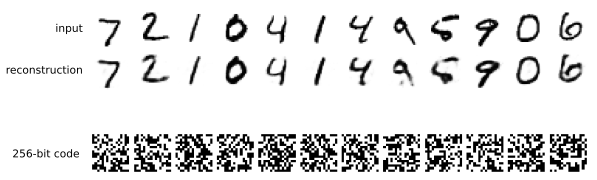
21.6.2 VQ-VAE model
pp. 815–817 A richer model uses a 3d tensor of discrete latents, \(\bm z\in\R^{H\times W\times K}\) with \(K\) values per latent position. Compare the continuous encoder output \(\bm z_e(\bm x)_{ij}\) with a codebook \(\{\bm e_k\in\R^D\}_{k=1}^K\) and pick the nearest entry: \[ q(z_{ij}=k\given\bm x)=\begin{cases}1&k=\arg\min_{k'}\|\bm z_e(\bm x)_{ij}-\bm e_{k'}\|_2\\0&\text{otherwise}\end{cases} \tag{21.76} \] and pass \((\bm z_q)_{ij}=\bm e_k\) when \(z_{ij}=k\) (21.77) to the decoder (Figure 21.16, a diagram). The distributed code is very expressive: a \(32\times32\) grid with \(K=512\) represents \(512^{32\times32}=2^{9216}\) distinct images. The negative log-likelihood is minimised by the straight-through estimator, which passes the decoder-input gradient \(\partial\mathcal L/\partial\bm z_q\) to the encoder output \(\bm z_e\), skipping (21.76). The codebook then receives no learning signal, so add the codebook loss with a stop-gradient operator \(\mathrm{sg}\): \[ \mathcal L=-\log p(\bm x\given\bm z_q(\bm x))+\|\mathrm{sg}(\bm z_e(\bm x))-\bm e\|_2^2. \tag{21.78} \] Alternatively, update the codebook by moving averages. For the \(n_i\) encoder outputs \(\bm z_{i,1},\dots,\bm z_{i,n_i}\) closest to \(\bm e_i\), minimising \(\sum_j\|\bm z_{i,j}-\bm e_i\|_2^2\) (21.79) has the closed form \(\bm e_i=\frac1{n_i}\sum_j\bm z_{i,j}\) (21.80), the M step of a Gaussian mixture. In minibatches, with \(n_i^t\) the count in the batch at step \(t\), \[ N_i^t=\gamma N_i^{t-1}+(1-\gamma)n_i^t,\qquad\bm m_i^t=\gamma\bm m_i^{t-1}+(1-\gamma)\sum_j\bm z_{i,j}^t,\qquad\bm e_i^t=\frac{\bm m_i^t}{N_i^t}, \tag{21.81--21.83} \] with \(\gamma=0.9\) working well. A third term, the commitment loss, keeps the encoder from changing its mind too often: \[ \mathcal L=-\log p(\bm x\given\bm z_q(\bm x))+\|\mathrm{sg}(\bm z_e(\bm x))-\bm e\|_2^2+\beta\|\bm z_e(\bm x)-\mathrm{sg}(\bm e)\|_2^2, \tag{21.84} \] with \(\beta=0.25\) working well (its value depends on the scale of the reconstruction loss). The decoder optimises only the first term, the encoder the first and the last, and the embeddings the middle term.
Filling the gap 21.15: the constant KL, straight-through and the three loss terms, the EMA codebook as a weighted mean, dead codes pp. 815–817, (21.75)–(21.84)
Proof
The KL is a constant. For a deterministic quantiser the posterior at each position is a point mass \(\delta_{k^*(\bm x)}\) and the prior is uniform, \(p(k)=1/K\): \(\Dkl=\sum_kq(k)\log\frac{q(k)}{p(k)}=\log\frac1{1/K}=\log K\) per position, whatever the input: the KL cannot be reduced by ignoring the code (no collapse), and it contributes no gradient. For the binary autoencoder of Section 21.6.1 there are \(K\) positions with \(S=2\) states, so the KL against the uniform prior on \(S^K\) codes is \(\log S^K=K\log S=K\log2\): 177.45 nats for \(K=256\), not \(\log K\) as printed in the book (where \(K\) means the number of latent variables, not the number of states).
Straight-through and which loss feeds which parameter. Write \(\bm z_q=\bm z_e+\mathrm{sg}(\bm e-\bm z_e)\): its value is \(\bm e\), and its Jacobian with respect to \(\bm z_e\) is the identity (the straight-through estimator, which is biased; what it estimates is analysed in gap 6.7) and with respect to \(\bm e\) is zero. The reconstruction loss \(\ell(\bm z_q)\) therefore gives the decoder its true gradient and the encoder \(\partial\ell/\partial\bm z_q\), and gives the codebook nothing. The codebook loss \(\|\mathrm{sg}(\bm z_e)-\bm e\|^2\) has gradient \(2(\bm e-\bm z_e)\) with respect to the assigned code only, and the commitment loss \(\beta\|\bm z_e-\mathrm{sg}(\bm e)\|^2\) has gradient \(2\beta(\bm z_e-\bm e)\) with respect to the encoder only. Verified by automatic differentiation on a random example: the encoder gradient equals the decoder gradient at \(\bm z_q\) plus \(2\beta(\bm z_e-\bm e)\), and the codebook gradient equals \(2\sum(\bm e-\bm z_e)\) over assigned outputs.
(21.79)–(21.80). \(\nabla_{\bm e}\sum_j\|\bm z_j-\bm e\|^2=2\sum_j(\bm e-\bm z_j)=0\) at \(\bm e=\frac1n\sum_j\bm z_j\); the objective is a strictly convex quadratic, so this is the unique global minimiser.
The EMA is a weighted mean. Unrolling (21.81)–(21.82) from \(N^0\) and \(\bm m^0\), \[ N_i^t=\gamma^tN_i^0+(1-\gamma)\sum_{s=1}^t\gamma^{t-s}n_i^s,\qquad\bm m_i^t=\gamma^t\bm m_i^0+(1-\gamma)\sum_{s=1}^t\gamma^{t-s}\sum_j\bm z_{i,j}^s, \] so \(\bm e_i^t=\bm m_i^t/N_i^t\) is a weighted mean of the initial code (weight \(\gamma^tN_i^0\), with \(\bm m^0=N^0\bm e^0\)) and every encoder output ever assigned to the code, each with weight \((1-\gamma)\gamma^{t-s}\): the sum of the weights is \(N^t\), so it is a proper average (a ratio of two exponential moving averages, consistent but biased for a finite window when the batches are noisy). Three limits: \(\gamma=0\) gives exactly one k-means step per update, the batch mean of the assigned points (21.80); \(\gamma\to1\) averages over a long history and moves slowly; and with full batches \(n_i^t\) is the cluster size, so \(N^t\) estimates the cluster size.
Dead codes do not move. If code \(i\) is never nearest to any output, \(n_i^s=0\) and the sums vanish: \(N_i^t=\gamma^tN_i^0\), \(\bm m_i^t=\gamma^t\bm m_i^0\), so \(\bm e_i^t=\bm e_i^0\) for all \(t\) (both numerator and denominator decay at the same rate) and \(N_i^t\) decays geometrically to 0. The EMA update cannot revive an unused code; in practice dead codes are re-initialised from random encoder outputs, a device the book does not discuss. This is what Figure 21.x5 and the demo show: a code started outside the data keeps its initial position and its \(N\) falls as \(0.9^t\) (after 60 steps \(2\times10^{-3}\)).
Numbers (full batch, \(n=800\) points from five Gaussian blobs, eight codes, six started near the origin and two far outside the data). After 60 steps the mean squared quantisation error is 0.1711 for \(\gamma=0.5\), 0.1971 for \(\gamma=0.9\) and 0.1987 for \(\gamma=0.99\); Lloyd's k-means from the same start reaches 0.1843. The error after 5 steps is 0.190, 0.219 and 0.302: a large \(\gamma\) is slower. With \(\gamma=0.5\) all eight codes end up in use and the error ends below the k-means value, whose iteration stops in a worse local minimum; with \(\gamma=0.9\) and 0.99 one of the two far codes is never used and stays at its starting point. The implementation matches the hand recursion exactly, and with \(\gamma=0\) matches one Lloyd step.
Capacity. \(512^{32\cdot32}=(2^9)^{1024}=2^{9216}\). \(\square\)
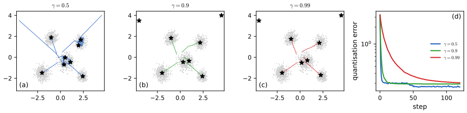
21.6.3 Learning the prior
p. 817 After training, a better prior can be fitted to the aggregated posterior: encode the data to discrete sequences \(\{\bm z_n\}\) and fit any sequence model to \(p(\bm z)\) (a causal-convolution PixelCNN in the original paper, transformer decoders more recently); samples are decoded by the VQ-VAE decoder.
21.6.4 Hierarchical extension (VQ-VAE-2)
pp. 817–818 VQ-VAE-2 (Razavi et al., 2019) uses a hierarchical code: on \(256\times256\times3\) images the first latent layer is \(64\times64\) and the second \(32\times32\), so the top level captures semantics and the lower level texture (Section 21.5). The prior over the top level is a PixelCNN with self-attention (PixelSNAIL), over the lower level a plain PixelCNN (attention would be too expensive); Figure 21.17 is a diagram.
21.6.5 Discrete VAE
p. 818 VQ-VAE uses a one-hot code, \(q(z=k\given\bm x)=1\) iff \(k=\arg\min_k\|\bm z_e(\bm x)-\bm e_k\|_2\), so it captures no uncertainty about the code and needs the straight-through estimator. The DALL-E model (Section 22.4.2) uses the Gumbel-softmax relaxation instead. A sample from \(q(z=k\given\bm x)\) is \(\arg\max_k g_k+\log q(z=k\given\bm x)\) with \(g_k\) Gumbel; the relaxation replaces the argmax by a softmax with temperature \(\tau>0\), \[ w_k=\frac{\exp\big((g_k+\log q(z=k\given\bm x))/\tau\big)}{\sum_{j=1}^K\exp\big((g_j+\log q(z=j\given\bm x))/\tau\big)},\qquad\bm z_q=\sum_{k=1}^Kw_k\bm e_k. \tag{21.85--21.86} \] As \(\tau\to0\) the weights become one-hot and \(\bm z_q\) a codebook entry; for finite \(\tau\) the space between the vectors is filled in. The objective is the usual differentiable one, \[ \mathcal L=-\E_{q(\bm z\given\bm x)}[\log p(\bm x\given\bm z)]+\beta\Dkl(q(\bm z\given\bm x)\|p(\bm z)), \tag{21.87} \] where, unlike VQ-VAE, the KL is not constant because the encoder is stochastic; the Gumbel noise is independent of the encoder parameters, so the reparameterisation trick (Section 6.3.5) applies.
Filling the gap 21.16: the Gumbel-max trick and the limits of the relaxation p. 818, (21.85)–(21.87)
Proof
The proof that \(\arg\max_kg_k+\log q_k\) is a sample from \(\Cat(\bm q)\) when the \(g_k\) are i.i.d. standard Gumbel, and the two limits of the relaxation (one-hot as \(\tau\to0\), uniform as \(\tau\to\infty\)), are in gap 6.6. Numerically, for \(\bm q=(0.1,0.2,0.3,0.4)\) and \(2\times10^5\) draws the argmax frequencies are \((0.100,0.200,0.302,0.399)\), at \(\tau=10^{-3}\) the largest weight exceeds 0.99 for over 98% of the draws (a draw lands near a tie with probability about \(\tau\)), and at \(\tau=10^3\) all weights are within 0.01 of \(1/4\). Two cautions beyond the book: the relaxed \(\bm z_q\) at finite \(\tau\) is a different model from the discrete one, so the resulting objective (21.87) is not a bound on the discrete model's log-likelihood unless \(\tau\) is annealed to zero (Maddison et al., 2017; Jang et al., 2017), and the book's notation uses \(w_k\) for both the sampled index and the relaxed weight. \(\square\)
21.6.6 VQ-GAN
p. 819 VQ-VAE's squared-error reconstruction loss gives blurry samples. VQ-GAN (Esser, Rombach and Ommer, 2021) replaces it by a patch-wise GAN loss (Chapter 26) with a perceptual loss, and models the latent prior with a transformer (Section 16.3.5; Figure 21.18 is a diagram); Yu et al. (2021) replace the CNN encoder and decoder by transformers (vector-quantised image modelling, VIM).
Practice problems
The book has no end-of-chapter exercises for Chapter 21, so here are three short problems of my own, with complete solutions (hidden).
Practice problem 21.1 (collapse in a one-dimensional linear VAE). Data \(x\sim\N(0,\lambda)\), decoder \(x\given z\sim\N(wz,\sigma^2)\), prior \(z\sim\N(0,1)\), encoder \(z\given x\sim\N(ax,s^2)\), loss \(\frac1{2\sigma^2}\E(x-wz)^2+\beta\,\E\Dkl\). (a) Show that the optimum is collapsed iff \(\lambda\le\beta\sigma^2\). (b) For \(\lambda=2\), \(\sigma^2=1\) find the optimal rate and error for \(\beta=1\) and \(\beta=2\). (c) With free bits \(\lambda_{\rm fb}=0.1\) on a collapsed unit (\(\lambda=0.5\), \(\sigma^2=1\), \(\beta=1\)), what happens and what is the loss?
Solution
(a) This is Result 21.1 with \(D=K=1\): \(f(u)=\frac{\lambda}{2\sigma^2u}+\frac\beta2\log u\) over \(u\ge1\) has \(f'(u)=\frac1{2u}(\beta-\frac{\lambda}{\sigma^2u})\), which is \(\ge0\) for all \(u\ge1\) iff \(\lambda\le\beta\sigma^2\); then \(u=1\) (rate 0, error \(\lambda\), \(a=0\), \(s=1\)). Otherwise \(u^*=\lambda/(\beta\sigma^2)\). (b) \(\beta=1\): \(u=2\), rate \(\frac12\log2=0.3466\), error \(\lambda/u=1=\beta\sigma^2\), loss \(\frac1{2}+0.3466=0.8466\). \(\beta=2\): \(\lambda=2=\beta\sigma^2\), the boundary: \(u=1\), rate 0, error 2, loss 1. Training the exact loss by gradient descent for \(\lambda=2\), \(\beta=1\) gives rate 0.3466 and for \(\lambda=0.2\) the collapse (rate \(10^{-17}\)). (c) With the hinge, a unit with KL below 0.1 costs a flat \(\beta\lambda_{\rm fb}=0.1\), so it should spend its free budget: \(\frac12\log u=0.1\), \(u=e^{0.2}=1.2214\) (a larger \(u\) is not worth it since \(u^*=\lambda/(\beta\sigma^2)=0.5<1\)). The error is \(0.5/1.2214=0.4094\) instead of 0.5, and the penalised loss \(\frac{0.4094}{2}+0.1=0.3047\), against \(0.25+0.1=0.35\) if it stayed at the prior (the hinge charges 0.1 even at KL 0). So free bits keep the unit alive at KL exactly \(\lambda_{\rm fb}\).
Practice problem 21.2 (product of experts with a missing modality). A one-dimensional latent has prior \(\N(0,1)\) and two modality experts \(\N(2,1)\) and \(\N(-1,\tfrac12)\) (mean, variance). (a) Find the posterior \(q(z\given\bm x_1,\bm x_2)\). (b) Find it if modality 2 is missing. (c) By how much does the posterior standard deviation grow?
Solution
The precisions are 1 (prior), 1 and 2. (a) By (21.47): precision \(1+1+2=4\), variance 0.25 (sd 0.5), mean \(\frac14(1\cdot0+1\cdot2+2\cdot(-1))=0\). (b) Drop the second expert: precision \(1+1=2\), variance 0.5, mean \(\frac12(0+2)=1\). (c) The sd rises from 0.5 to \(0.7071\) (by 41%), and the mean moves from 0 to 1, because the missing expert was the one pulling to the left; the posterior with fewer modalities is wider and located where the remaining evidence puts it. Computed with
poein the code.Practice problem 21.3 (the MMD between two Gaussians). With \(K(z,z')=e^{-(z-z')^2/2}\) (\(s=1\)) in one dimension, compute \(\mathrm{MMD}^2\) between \(\N(0,1)\) and \(\N(\delta,1)\) from (21.38). Evaluate at \(\delta=1.3\), find its behaviour for small \(\delta\), and compare with an estimate from 3 000 draws of each.
Solution
Use the closed form of gap 21.7 with \(d=1\), \(s^2=1\): \(\E K=(1+\Sigma_1+\Sigma_2)^{-1/2}\exp(-\frac{(m_1-m_2)^2}{2(1+\Sigma_1+\Sigma_2)})\), with \(\Sigma_1+\Sigma_2=2\) for the two Gaussians and the within-distribution pairs. For \(pp\) and \(qq\): \(m_1=m_2\), so \(\E K=1/\sqrt3\) each. For \(pq\): \(\E K=\frac1{\sqrt3}e^{-\delta^2/6}\). Hence \(\mathrm{MMD}^2=\frac2{\sqrt3}-\frac2{\sqrt3}e^{-\delta^2/6}=\frac2{\sqrt3}(1-e^{-\delta^2/6})\). At \(\delta=1.3\): \(\delta^2/6=0.2817\), \(e^{-0.2817}=0.7544\), \(\mathrm{MMD}^2=1.1547\times0.2456=0.2835\). For small \(\delta\), \(\mathrm{MMD}^2\approx\frac{\delta^2}{3\sqrt3}=0.1925\,\delta^2\): quadratic in \(\delta\), so \(\mathrm{MMD}\) (the square root) is linear. For large \(\delta\) it saturates at \(2/\sqrt3\): the kernel cannot tell apart distributions that are far apart, a reason to choose the bandwidth with care (gap 2.28). The estimator (21.38) with 3 000 draws from each (the biased V-statistic of the code) gives 0.278, within the sampling error of the exact value.
Demonstrations
- Reverse water-filling in a linear β-VAE (Sections 21.3.1, 21.4): \(\beta\), \(\sigma^2\) and the spectrum; which directions are used, the rate and error of each, and the rate-distortion curve.
- The latent plane of a VAE (Sections 21.2.3, 21.3.1): decode any point of an autoencoder or a \(\beta\)-VAE with two latent dimensions, interpolate, draw from the prior; rate, its split and the hole fraction.
- The VQ-VAE codebook and its moving-average update (Section 21.6.2): \(\gamma\), minibatch size and start; dead codes and the k-means comparison.
Python code for every figure: code index. Data used by the demos: data/ch21-linear.json, data/ch21-latent-ae.json, 0p25, 1, 4, data/ch21-vq.json. Companion demos: Volume 1 (PCA and factor analysis), the deep-learning course.
Notes on the book
Points where the book is imprecise or wrong
- (21.7). With \(\bm\ell=\log\bm\sigma\), \(\diag(\exp\bm\ell)\) is \(\diag(\bm\sigma)\); the covariance is \(\diag(\exp(2\bm\ell))\). The same convention slip is in (21.50)–(21.54).
- Section 21.2.1. "Convergence to a locally optimal MLE of the parameters is guaranteed" is too strong: stochastic gradient ascent on the ELBO converges to a stationary point of the ELBO, which is stationary for the likelihood only if \(q\) is the posterior (gap 21.1).
- Algorithm 21.1, line 6.
M = np.triu(np.ones(K), -1)is not strictly lower triangular; it should benp.tril(np.ones(K), -1), otherwise \(\det\bm L\ne\prod_k\sigma_k\) and line 10 is not \(\log q\) (gap 21.2). - Algorithm 21.1, line 13. With
Llogpxdefined as the negative log-likelihood andLlogqz,Llogpzas log-densities, \(\mathcal L=\)Llogpx + Llogpz - Llogqzcarries the wrong sign on the prior and entropy terms; the negative ELBO isLlogpx - Llogpz + Llogqz(printed value \(-4.38\) against \(12.14\) on a test example). - (21.19)–(21.22). With \(p_{\mathcal D}\) the empirical (delta) distribution, \(\Dkl(p_{\mathcal D}\|p_{\bm\theta})\) and \(\E\log p_{\mathcal D}\) are infinite for continuous data; the identities are for a population density, and the "up to a constant" in (21.20)–(21.22) hides infinities. (21.20) writes \(q_{\bm\phi}(\bm x,\bm z)\) for \(q_{\mathcal D,\bm\phi}(\bm x,\bm z)\).
- (21.52) versus (21.56). The unlabelled posterior is written \(q(\bm z\given\bm x)q(y\given\bm x)\), but (21.56) is the bound for \(q(y\given\bm x)q(\bm z\given\bm x,y)\) (gap 21.10).
- Section 21.6.1. "The KL divergence reduces to a constant, equal to \(\log K\)": with \(K\) binary latents against a uniform prior it is \(K\log2\) (177.4 nats for the 256 bits of Figure 21.15), not \(\log K\) (\(=5.5\)); \(\log K\) holds per position for a codebook of \(K\) entries (gap 21.15).
- (21.85). \(w_k\) denotes both the (hard) sample \(w_k\sim q(z=k\given\bm x)\) and the relaxed weight; the first should be an index \(k^*=\arg\max_kg_k+\log q(z=k\given\bm x)\).
- Section 21.4 and footnote 5. The text attributes collapse to a powerful decoder and the footnote adds linear models; the exact condition for the linear case (\(\lambda_i\le\beta\sigma^2\)) and the fact that collapse is a global optimum in both cases are in gap 21.5 and gap 21.11.
References
- Murphy, K. P. (2023). Probabilistic Machine Learning: Advanced Topics. MIT Press, Cambridge, MA. Chapter 21, pp. 791–819, and supplementary material, Chapter 21. probml.github.io/pml-book/book2.html.
- Achille, A. and Soatto, S. (2018). Information dropout: learning optimal representations through noisy computation. IEEE Transactions on Pattern Analysis and Machine Intelligence, 40(12), 2897–2905.
- Bowman, S. R., Vilnis, L., Vinyals, O., Dai, A. M., Jozefowicz, R. and Bengio, S. (2016). Generating sentences from a continuous space. Conference on Computational Natural Language Learning.
- Child, R. (2021). Very deep VAEs generalize autoregressive models and can outperform them on images. International Conference on Learning Representations.
- Collier, M., Nazabal, A. and Williams, C. K. I. (2020). VAEs in the presence of missing data. ICML Workshop on the Art of Learning with Missing Values.
- Dai, B., Wang, Z. and Wipf, D. (2020). The usual suspects? Reassessing blame for VAE posterior collapse. International Conference on Machine Learning.
- Dayan, P., Hinton, G. E., Neal, R. M. and Zemel, R. S. (1995). The Helmholtz machine. Neural Computation, 7(5), 889–904.
- Dieng, A. B., Kim, Y., Rush, A. M. and Blei, D. M. (2019). Avoiding latent variable collapse with generative skip models. AISTATS.
- Esser, P., Rombach, R. and Ommer, B. (2021). Taming transformers for high-resolution image synthesis. IEEE/CVF Conference on Computer Vision and Pattern Recognition.
- Fu, H., Li, C., Liu, X., Gao, J., Celikyilmaz, A. and Carin, L. (2019). Cyclical annealing schedule: a simple approach to mitigating KL vanishing. NAACL.
- Gretton, A., Borgwardt, K. M., Rasch, M. J., Schölkopf, B. and Smola, A. (2012). A kernel two-sample test. Journal of Machine Learning Research, 13, 723–773.
- Ha, D. and Eck, D. (2018). A neural representation of sketch drawings. International Conference on Learning Representations.
- He, J., Spokoyny, D., Neubig, G. and Berg-Kirkpatrick, T. (2019). Lagging inference networks and posterior collapse in variational autoencoders. International Conference on Learning Representations.
- Higgins, I., Matthey, L., Pal, A., Burgess, C., Glorot, X., Botvinick, M., Mohamed, S. and Lerchner, A. (2017). β-VAE: learning basic visual concepts with a constrained variational framework. International Conference on Learning Representations.
- Jang, E., Gu, S. and Poole, B. (2017). Categorical reparameterization with Gumbel-softmax. International Conference on Learning Representations. Maddison, C. J., Mnih, A. and Teh, Y. W. (2017). The concrete distribution. International Conference on Learning Representations.
- Kingma, D. P. and Welling, M. (2014). Auto-encoding variational Bayes. International Conference on Learning Representations. Kingma, D. P. and Welling, M. (2019). An introduction to variational autoencoders. Foundations and Trends in Machine Learning, 12(4), 307–392.
- Kingma, D. P., Mohamed, S., Rezende, D. J. and Welling, M. (2014). Semi-supervised learning with deep generative models. Advances in Neural Information Processing Systems, 27. Kingma, D. P., Salimans, T., Jozefowicz, R., Chen, X., Sutskever, I. and Welling, M. (2016). Improved variational inference with inverse autoregressive flow. Advances in Neural Information Processing Systems, 29.
- Little, R. J. A. and Rubin, D. B. (1987). Statistical Analysis with Missing Data. Wiley.
- Locatello, F., Bauer, S., Lucic, M., Rätsch, G., Gelly, S., Schölkopf, B. and Bachem, O. (2019). Challenging common assumptions in the unsupervised learning of disentangled representations. International Conference on Machine Learning.
- Lucas, J., Tucker, G., Grosse, R. and Norouzi, M. (2019). Don't blame the ELBO! A linear VAE perspective on posterior collapse. Advances in Neural Information Processing Systems, 32.
- Makhzani, A., Shlens, J., Jaitly, N., Goodfellow, I. and Frey, B. (2015). Adversarial autoencoders. arXiv:1511.05644.
- van den Oord, A., Vinyals, O. and Kavukcuoglu, K. (2017). Neural discrete representation learning. Advances in Neural Information Processing Systems, 30. Razavi, A., van den Oord, A. and Vinyals, O. (2019). Generating diverse high-fidelity images with VQ-VAE-2. Advances in Neural Information Processing Systems, 32.
- Rezende, D. J., Mohamed, S. and Wierstra, D. (2014). Stochastic backpropagation and approximate inference in deep generative models. International Conference on Machine Learning.
- Sønderby, C. K., Raiko, T., Maaløe, L., Sønderby, S. K. and Winther, O. (2016). Ladder variational autoencoders. Advances in Neural Information Processing Systems, 29.
- Tipping, M. E. and Bishop, C. M. (1999). Probabilistic principal component analysis. Journal of the Royal Statistical Society B, 61(3), 611–622.
- Vahdat, A. and Kautz, J. (2020). NVAE: a deep hierarchical variational autoencoder. Advances in Neural Information Processing Systems, 33.
- Vedantam, R., Fischer, I., Huang, J. and Murphy, K. (2018). Generative models of visually grounded imagination. International Conference on Learning Representations.
- Wu, M. and Goodman, N. (2018). Multimodal generative models for scalable weakly-supervised learning. Advances in Neural Information Processing Systems, 31.
- Xu, J. and Durrett, G. (2018). Spherical latent spaces for stable variational autoencoders. EMNLP. Davidson, T. R., Falorsi, L., De Cao, N., Kipf, T. and Tomczak, J. M. (2018). Hyperspherical variational auto-encoders. Uncertainty in Artificial Intelligence.
- Razavi, A., van den Oord, A., Poole, B. and Vinyals, O. (2019). Preventing posterior collapse with delta-VAEs. International Conference on Learning Representations.
- Yu, J. et al. (2021). Vector-quantized image modeling with improved VQGAN.
- Zhao, S., Song, J. and Ermon, S. (2019). InfoVAE: balancing learning and inference in variational autoencoders. AAAI.
The numerical statements in the text (the discrete-model identities for the four forms of the ELBO, the rate split, the total correlation and the InfoVAE rewriting; the Gaussian product of experts and its exactness; the M2 bound; the conditional-mean decoder; the water-filling optimum, its link to probabilistic PCA and its collapse threshold; the corrected Algorithm 21.1; the hierarchical ELBO and the residual KL; the autoregressive limit; the Gumbel-softmax limits; the EMA codebook, dead codes and straight-through gradients; the closed-form MMD; and the trained-network numbers) were confirmed numerically.