Bayesian neural networks
A neural network trained by maximum likelihood returns one function; a Bayesian neural network returns a whole distribution over functions and averages the predictions of all of them. The averaging is exact in theory and out of reach in practice, so the chapter is a tour of priors (what functions does a Gaussian prior on the weights prefer?), of approximate posteriors (Laplace, variational inference, Hamiltonian Monte Carlo, SGD iterates, ensembles), of why averaging helps generalisation (flat minima, effective dimension, PAC-Bayes) and fails when the prior is poor, and of sequential updating with the extended Kalman filter, assumed density filtering and variational continual learning.
Ch. 1 Introduction Ch. 2 Probability Ch. 3 Statistics Ch. 4 Graphical models Ch. 5 Information theory Ch. 6 Optimisation Ch. 7 Inference algorithms Ch. 8 Gaussian filtering Ch. 9 Message passing Ch. 10 Variational inference Ch. 11 Monte Carlo Ch. 12 MCMC Ch. 13 Sequential Monte Carlo Ch. 14 Predictive models Ch. 15 GLMs Ch. 16 Deep networks Ch. 17 Bayesian neural networks Ch. 18 Gaussian processes Ch. 19 Beyond iid Ch. 20 Generative models Ch. 21 VAEs Ch. 22 Autoregressive models Ch. 23 Normalizing flows Ch. 24 Energy-based models Ch. 25 Diffusion models Ch. 26 GANs Ch. 27 Discovery methods Ch. 28 Latent factor models Ch. 29 State-space models Ch. 30 Graph learning Ch. 31 Nonparametric Bayes Ch. 32 Representation learning Ch. 33 Interpretability Ch. 34 Decision making Ch. 35 Reinforcement learning Ch. 36 Causality
How to read these notes
They follow the book. Sections carry the book's numbers (17.2, 17.3.8, ...) and displayed equations that appear in the book carry its equation numbers, e.g. \((17.1)\). Equations without a number are steps the book skips. Sections of the online supplement are labelled "(supplement)" and placed where the book refers to them.
Filling the gaps. Wherever the book states a result without proof, leaves a calculation to the reader or quotes the literature, an orange Filling the gap box gives the argument. Derivations start hidden: open one with its bar, or use the button below. Results already proved in full in the companion courses are stated and linked rather than repeated.
Figures and demonstrations. Every figure of the chapter that is computed from data, a model or a simulation is reproduced from scratch by the Python code, apart from those that need GPU-scale training (Figures 17.12 and 17.14) or a large pretrained network (17.9), and the diagrams and sketches (17.3, 17.5, 17.6, 17.8, 17.10, 17.13, 17.18). Figures 17.S1 to 17.S8 are extra ones made for the gaps. The ▶ Demo boxes open an interactive demonstration already set to the case under discussion.
Main reference
K. P. Murphy, Probabilistic Machine Learning: Advanced Topics, MIT Press (2023; the December 2025 draft is followed), Chapter 17 (coauthored with Andrew Wilson), pages 647–680, and Supplementary Section 17.1, pages 181–182 of the supplement (book web page: probml.github.io/pml-book/book2.html). Section, equation, figure and algorithm numbers refer to this book. Chapter 17 has no end-of-chapter exercises, so three practice problems with solutions are given instead.
The explanations, derivations, figures and code are my own; equations are cited by their numbers in the book.
Companion courses
This chapter uses material that is developed elsewhere on this site, and the proofs there are not repeated here:
- The Laplace approximation, evidence maximisation and Bayesian networks in Bishop's notation: Bayesian and Probabilistic ML, Section 5.7.
- Fixed-form variational inference and the reparameterisation trick, expectation propagation: Section 10.2, 10.2.1 and 10.7 of the Chapter 10 notes.
- Hamiltonian Monte Carlo, stochastic gradient Langevin dynamics and SGD as a Langevin sampler, the non-centred parameterisation: Section 12.5, 12.7.1, Filling the gap 12.15 and Section 12.6.5 of the Chapter 12 notes.
- The extended Kalman filter and assumed density filtering (including ADF for DNNs): Section 8.3.2, 8.6.3 and 8.6.4; the Laplace approximation in general: Section 7.4.3; empirical Bayes and the marginal likelihood: Section 3.7 and 3.8.
- Neural networks and dropout in the first volume: Probabilistic Machine Learning: An Introduction, Chapter 13.
New here: the variance recursion behind Xavier and LeCun scaling, evidence maximisation and the effective dimension, why MC dropout does not shrink with the data, the generalised Gauss–Newton and linearised Laplace predictive, the local reparameterisation trick, random features and spectral normalisation, the weight-space symmetries of the posterior, the stationary law of constant-step SGD and the SWA average, randomize-then-optimise ensembles, the Laplace bridge, tempering and the Gibbs variational principle, the Occam factor and reparameterisation, the McAllester-type PAC-Bayes proof, the posterior-equals-prior phenomenon behind poor BMA under shift, ReLU overconfidence, sequential Laplace and EWC, the EKF as a Gauss–Newton step, the ADF moment formulas, the GVCL limit and the decoupled and mini-batch EKF of the supplement.
The chapter at a glance
- 17.1–17.2 Bayesian model averaging is the log-loss optimal predictor and its gain is the epistemic uncertainty (Result 17.1); a Gaussian prior on the weights is a prior on functions whose scale is set by the layer variances (Filling the gap 17.2); evidence maximisation (17.3).
- 17.3 MC dropout does not concentrate (17.4); the generalised Gauss–Newton and the linearised predictive (17.5); Bayes by backprop and local reparameterisation (17.6); the probit integral and last-layer methods (17.7); random features and spectral normalisation (17.8); symmetries of the posterior (17.9); constant-step SGD and SWA (17.10); random-prior ensembles (17.11); batch ensemble (17.12); the Laplace bridge (17.13); distillation (17.14); tempering (17.15).
- 17.4 The Occam factor and reparameterisation (17.16); the effective dimension (17.17); the conservation of evidence (17.18); PAC-Bayes (17.19); poor BMA under shift (17.20); ReLU overconfidence (17.21).
- 17.5–17.6 Sequential Laplace and EWC (17.22); the EKF as a Gauss–Newton step (17.23); the decoupled and mini-batch EKF of the supplement (17.24, 17.25); ADF (17.26); variational continual learning (17.27); partial pooling (17.28).
Notation. \(\th\) is the vector of all weights and biases, \(P\) its length, \(f(\bm x;\th)\) the network output (the logits for classification), \(\mathcal D=\{(\bm x_n,y_n)\}_{n\le N}\) the data, \(p(\th)\) the prior and \(p(\th\given\mathcal D)\propto p(\mathcal D\given\th)p(\th)\) the posterior. \(\bm J_{\th}(\bm x)=\partial f/\partial\th\) is the Jacobian (the book is not consistent about \(C\times P\) against \(P\times C\); these notes use \(C\times P\)).
Prerequisites. Gaussian conditioning and the Bayesian linear model (Chapters 2 and 3), the ELBO and the Laplace approximation (Chapters 7 and 10), Hamiltonian Monte Carlo (Chapter 12).
17.1 Introduction
p. 647, (17.1) A network trained by (penalised) maximum likelihood returns one parameter vector, although many settings fit the training set equally well and generalise differently (underspecification, Figure 17.11). The Bayesian alternative averages their predictions with the posterior as weights,
\[ p(y\given\bm x,\mathcal D)=\int p(y\given\bm x,\th)\,p(\th\given\mathcal D)\,\d\th,\qquad p(\th\given\mathcal D)\propto p(\th)\,p(\mathcal D\given\th). \tag{17.1}\]Two obstacles dominate: choosing a prior (Section 17.2) and computing or approximating a posterior over millions of parameters (Section 17.3). "Bayesian deep learning" (BDL) is Bayesian inference for network weights; "deep Bayesian learning" (DBL) is the use of networks to speed up inference for classical models (amortised inference, Section 10.1.5).
Result 17.1 (why average? the log-loss optimality of the posterior predictive and the epistemic term) p. 647, (17.1)
Let \(\th\sim p(\th\given\mathcal D)\) and \(y\given\th\sim p(y\given\bm x,\th)\). (a) Among all densities \(q(y)\), the posterior predictive \(\bar p=p(y\given\bm x,\mathcal D)\) minimises the expected log loss \(\E_\th\E_{y\given\th}[-\log q(y)]\), and the minimum is the entropy \(\mathbb H[\bar p]\). (b) With \(\mathbb I(y;\th\given\bm x,\mathcal D)\) the mutual information between the output and the weights, \[ \mathbb H[\bar p]=\E_\th\,\mathbb H[p(y\given\bm x,\th)]+\mathbb I(y;\th\given\bm x,\mathcal D)\ \ge\ \E_\th\,\mathbb H[p(y\given\bm x,\th)]. \] (c) Consequently the log loss of any equally weighted mixture of \(M\) models is at most the average of their log losses, and for a Gaussian likelihood the predictive variance splits as \[ \var[y]=\E_\th[\sigma^2(\bm x,\th)]+\var_\th[\mu(\bm x,\th)] \] (aleatoric plus epistemic).
Filling the gap 17.1: proof of Result 17.1 p. 647
The book asserts that "considering all of these models together can lead to improved accuracy and uncertainty representation"; this is the precise sense.
Derivation
(a) Taking the expectation over \(\th\) first, \[ \E_\th\E_{y\given\th}[-\log q(y)]=\E_{y\sim\bar p}[-\log q(y)] \] because \(\bar p=\int p(y\given\th)p(\th\given\mathcal D)\d\th\) is the marginal of \(y\). Then \[ \E_{\bar p}[-\log q]=\mathbb H[\bar p]+\KL(\bar p\,\|\,q)\ge\mathbb H[\bar p] \] with equality iff \(q=\bar p\) (Gibbs' inequality, Section 5.1).
(b) By definition \(\mathbb I(y;\th)=\mathbb H[y]-\mathbb H[y\given\th]\), with \(\mathbb H[y]=\mathbb H[\bar p]\) and \(\mathbb H[y\given\th]=\E_\th\mathbb H[p(y\given\th)]\); \(\mathbb I\ge0\) because it is a KL divergence between the joint and the product of the marginals.
(c) Applying (a) to a discrete posterior that puts mass \(1/M\) on each of \(M\) models gives \[ -\log\big(\tfrac1M\sum_mp_m(y)\big)\le\tfrac1M\sum_m(-\log p_m(y)) \] pointwise, which is Jensen's inequality for the convex function \(-\log\). The gap is exactly the mutual information between \(y\) and the model index. For a Gaussian likelihood \(p(y\given\bm x,\th)=\N(\mu(\bm x,\th),\sigma^2(\bm x,\th))\) the law of total variance gives the stated split.
These identities are exact for the posterior mean over \(\th\); every method of Section 17.3 replaces the posterior by an approximation \(q\), and then (a) holds with \(\bar p\) replaced by the predictive of \(q\). The mutual information term is the epistemic uncertainty: it vanishes when all posterior draws agree, which is what a point estimate (and, as shown in Filling the gap 17.4, MC dropout on a large data set) wrongly assumes.
17.2 Priors for BNNs
p. 647 To do Bayesian inference for a network we must choose \(p(\th)\). The common choices are summarised here.
17.2.1 Gaussian priors
pp. 648–650, (17.2)–(17.11), Figure 17.1 An MLP with \(L-1\) hidden layers and a linear output is \[ f(\bm x;\th)=\bm W_L\,\phi(\cdots\phi(\bm W_1\bm x+\bm b_1))+\bm b_L \] (17.2)–(17.4), and the standard prior is factored Gaussian,
\[ \bm W_\ell\sim\N(\bm 0,\alpha_\ell^2\bm I),\quad \bm b_\ell\sim\N(\bm 0,\beta_\ell^2\bm I),\qquad \alpha_\ell^2=\frac{2}{n_{\rm in}+n_{\rm out}}\ \text{(Xavier)},\quad \alpha_\ell^2=\frac1{n_{\rm in}}\ \text{(LeCun)}. \tag{17.5--17.7}\]Writing \(\bm W_\ell=\alpha_\ell\bm\eta_\ell\) and \(\bm b_\ell=\beta_\ell\bm\epsilon_\ell\) with standard normal \(\bm\eta,\bm\epsilon\) (17.8) turns every setting of \((\alpha,\beta)\) into a random function (17.9). Figure 17.1 draws ten such functions for a scalar-input, scalar-output MLP with twelve sigmoid hidden units.
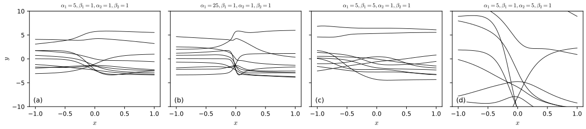
fig_17_1. Reproduces Murphy (2023), Figure 17.1. Download: PDF · SVGFilling the gap 17.2: what the scales do, and where Xavier, LeCun and the ReLU rescaling (17.10)–(17.11) come from pp. 648–649
The book describes the effect of \(\alpha_1,\beta_1,\alpha_2\) in words and quotes the initialisations. All of it follows from the distribution of one pre-activation.
Derivation
The exact law of a pre-activation. Given the previous layer's output \(\bm z\in\R^{n_{\rm in}}\), the pre-activation \(a_i=\sum_jW_{ij}z_j+b_i\) is a linear combination of independent Gaussians, hence \(a_i\given\bm z\sim\N(0,\ \alpha^2\|\bm z\|^2+\beta^2)\), exactly and independently across \(i\). For the output of the one-hidden-layer MLP (scalar input and output, \(H\) units) the prior variance of \(f(x)\) is therefore \[ \var f(x)=H\alpha_2^2\,\E[\phi(u)^2]+\beta_2^2,\qquad u\sim\N(0,\alpha_1^2x^2+\beta_1^2), \] because the \(H\) terms \(W_{2j}\phi(u_j)\) are independent with mean zero. So \(\alpha_2\) scales the standard deviation of the functions linearly (panel (d); with five times larger \(\alpha_2\) the standard deviation is about five times larger once \(H\alpha_2^2\E\phi^2\) dominates \(\beta_2^2\)).
Steps and their centres. A sigmoid unit \(\sigma(w x+b)\) with \(w=\alpha_1\eta\), \(b=\beta_1\epsilon\) has its centre at \(x_c=-b/w\). The ratio of two independent standard normals is Cauchy, so \(x_c\sim\mathrm{Cauchy}(0,\beta_1/\alpha_1)\) and the proportion of units whose centre lies in \([-1,1]\) is \(\tfrac2\pi\arctan(\alpha_1/\beta_1)\): 87% for \(\alpha_1/\beta_1=5\), 97.5% for 25 and 50% for \(\alpha_1/\beta_1=1\). This is the content of panels (b) and (c): raising \(\alpha_1\) sharpens the steps and keeps them inside the plotting window, raising \(\beta_1\) pushes most centres outside it, leaving nearly constant functions. The width of a step is \(1/|w|\sim1/\alpha_1\).
Variance preservation (LeCun, Xavier). Let \(q_\ell=\E[a_i^2]\) be the second moment of a pre-activation in layer \(\ell\), with \(\beta=0\). For large width the average \(\|\bm z\|^2/n_{\rm in}\) concentrates on \(m_{\ell-1}=\E\phi(a)^2\) with \(a\sim\N(0,q_{\ell-1})\) (law of large numbers), so \[ q_\ell=\alpha_\ell^2\,n_{\rm in}\,m_{\ell-1}. \] With \(\alpha^2=1/n_{\rm in}\) (LeCun) this is \(q_\ell=m_{\ell-1}\): the signal variance is preserved when \(\phi\) is the identity or when \(\phi\) is close to the identity on the typical range (tanh), and is halved by each ReLU layer, since \(\E[\max(a,0)^2]=q/2\) for symmetric \(a\); this is why the ReLU-adapted value is \(2/n_{\rm in}\). The backward pass (gradients) multiplies by \(\bm W^\T\), so the same argument asks for \(\alpha^2=1/n_{\rm out}\). Xavier's \(2/(n_{\rm in}+n_{\rm out})\) is the harmonic mean of the two requirements.
The ReLU rescaling. If every \(\beta_\ell=0\) then \[ f(\bm x;\bm\alpha)=\alpha_L\bm\eta_L\phi(\cdots\phi(\alpha_1\bm\eta_1\bm x)) \]. The ReLU is positively homogeneous, \(\phi(cz)=c\,\phi(z)\) for \(c>0\) (the book's remark about negative \(\alpha\) is unnecessary, because \(\alpha_\ell\) is a standard deviation and is positive), so the scales factor out: \[ f(\bm x;\bm\alpha,\bm 0)=\alpha_L\cdots\alpha_1\,f(\bm x;\bm 1,\bm 0) \] (17.10)–(17.11). With non-zero biases the relative size of \(\alpha\) and \(\beta\) matters, because \(\phi(\alpha z+\beta)\ne\alpha\,\phi(z+\beta/\alpha)\) unless \(\phi\) is homogeneous and the bias is scaled too. These formulas were confirmed numerically.
17.2.2 Sparsity-promoting priors
p. 650 A Laplace prior \(p(w)=\frac1{2b}e^{-|w|/b}\) makes the negative log posterior \(-\log p(\mathcal D\given\th)+\frac1b\|\th\|_1+\mathrm{const}\), so the MAP estimate is the \(\ell_1\)-penalised (lasso) fit and many weights are exactly zero; for channels in a CNN a group version is used. The Gaussian prior gives the \(\ell_2\) penalty (weight decay) \(\frac1{2\alpha^2}\|\th\|^2\).
17.2.3 Learning the prior
p. 650, (17.12) Grid search over the prior scales by cross-validation grows exponentially with their number. Empirical Bayes maximises the marginal likelihood (the evidence), \[ \log p(\mathcal D\given\alpha,\beta)=\log\int p(\mathcal D\given\th)p(\th\given\alpha,\beta)\d\th \] (17.12), by gradient ascent; this can switch off irrelevant weights (automatic relevance determination). The integral is intractable for large networks, but for a model that is linear in the weights it has a closed form, and the Laplace approximation gives the same structure for a network.
Filling the gap 17.3: evidence maximisation for the prior scale, and the effective number of parameters p. 650, (17.12)
The book describes the method; here is the fixed-point update and its meaning, for the linear-in-the-weights case (a last layer, or a linearised network).
Derivation
Model. \(\bm y=\bm\Phi\bm w+\bm\varepsilon\), \(\bm w\sim\N(\bm 0,\alpha^{-1}\bm I_P)\) (\(\alpha\) is a precision here), \(\bm\varepsilon\sim\N(\bm 0,\sigma^2\bm I_N)\). Let \(\bm A=\alpha\bm I+\bm\Phi^\T\bm\Phi/\sigma^2\) and \(\bm m=\bm A^{-1}\bm\Phi^\T\bm y/\sigma^2\) (posterior precision and mean). Completing the square gives \[ \log p(\bm y\given\alpha)=-E(\bm m)+\tfrac P2\log\alpha-\tfrac12\log|\bm A|-\tfrac N2\log(2\pi\sigma^2),\qquad E(\bm w)=\tfrac\alpha2\|\bm w\|^2+\tfrac1{2\sigma^2}\|\bm y-\bm\Phi\bm w\|^2. \]
Derivative. Because \(\bm m\) minimises \(E\), the dependence of \(\bm m\) on \(\alpha\) does not contribute (envelope theorem), so \(\partial E(\bm m)/\partial\alpha=\tfrac12\|\bm m\|^2\). Also \(\partial\log|\bm A|/\partial\alpha=\Tr\bm A^{-1}\). With \(\lambda_i\) the eigenvalues of \(\bm\Phi^\T\bm\Phi/\sigma^2\), \(\Tr\bm A^{-1}=\sum_i(\lambda_i+\alpha)^{-1}\) and \[ \frac{P}{\alpha}-\Tr\bm A^{-1}=\sum_i\Big(\frac1\alpha-\frac1{\lambda_i+\alpha}\Big)=\frac1\alpha\sum_i\frac{\lambda_i}{\lambda_i+\alpha}=\frac\gamma\alpha,\qquad \gamma=\sum_{i=1}^P\frac{\lambda_i}{\lambda_i+\alpha}. \] Hence \[ \partial_\alpha\log p(\bm y\given\alpha)=\tfrac12(\gamma/\alpha-\|\bm m\|^2) \], which vanishes at the fixed point \[ \alpha=\frac{\gamma}{\|\bm m\|^2}. \] The iteration (re-estimate \(\bm m\), \(\gamma\), then \(\alpha\)) is MacKay's update.
Meaning of \(\gamma\). In the eigenbasis of \(\bm\Phi^\T\bm\Phi/\sigma^2\) direction \(i\) has prior variance \(1/\alpha\) and posterior variance \(1/(\lambda_i+\alpha)\); the fraction of the prior variance removed by the data is \(\lambda_i/(\lambda_i+\alpha)\in(0,1)\). So \(\gamma\) counts the well-determined parameters, and the update says that the prior variance of the weights equals the average squared size \(\|\bm m\|^2/\gamma\) of the well-determined ones. The same \(\gamma\), with \(\lambda_i\) the Hessian eigenvalues at a mode and \(\alpha\to c\), is the effective dimensionality (17.36) of Section 17.4.3; Filling the gap 17.17 relates it to the degrees of freedom of ridge regression. For a network, replacing the evidence by its Laplace approximation (17.16) with the generalised Gauss–Newton matrix for the Hessian gives the same update with \(\lambda_i\) the eigenvalues of \(\sum_n\bm J_n^\T\bm\Lambda_n\bm J_n\) (Immer et al. 2021). Per-weight precisions \(\alpha_i=\gamma_i/m_i^2\) give automatic relevance determination: directions with \(\lambda_i\ll\alpha_i\) are driven to zero. A numerical experiment confirms the fixed point maximises the exact evidence.
See also: evidence maximisation for a network with Bishop's notation: Bayesian and Probabilistic ML, Section 5.7.2.
p. 650 Learning is more meaningful on a separate but related data set. Sun et al. (2022) fit a point estimate \(\hat\th_1\) on a large data set \(\mathcal D_1\), derive an approximate low-rank Gaussian posterior with SWAG (Section 17.3.8) and use it as the prior when fine-tuning on \(\mathcal D_2\) (a MAP estimate or an MCMC posterior): "Bayesian transfer learning".
17.2.4 Priors in function space
p. 650 The map from a weight prior to a function prior is opaque. One can instead choose priors from desired invariances, encode locality, independence and symmetry with residual pathway priors (Finzi et al. 2021), or use kernel methods and Gaussian processes (Chapter 18) to state a prior directly on functions.
17.2.5 Architectural priors
p. 651 The architecture can matter more than the weight distribution: a CNN encodes translation equivariance and hierarchy, an RNN sequential structure, and neural architecture search is a form of structural prior learning. Untrained networks with the right structure already work: the deep image prior (Ulyanov et al. 2018) denoises, inpaints and super-resolves with a random CNN, random CNNs recognise faces (Pinto and Cox 2012) and give features that help kernel methods (Zhang et al. 2017).
17.3 Posteriors for BNNs
p. 651 The posterior \(p(\th\given\mathcal D)\) of a network is never available in closed form, so every method below approximates it or the predictive (17.1). They differ in what they assume (a local Gaussian, a factorised Gaussian, a set of modes) and in cost. Section 17.4.6.2 compares eight of them on one example (Figure 17.15), and the posterior-comparison demonstration lets you compare several against a long HMC run on a one-dimensional problem.
17.3.1 Monte Carlo dropout
pp. 651–652, (17.13), Figure 17.2 Dropout multiplies each hidden unit by a Bernoulli mask during training. Monte Carlo dropout (Gal and Ghahramani 2016) keeps the masks at test time and averages the predictive distributions of \(S\) random sub-networks,
\[ p(y\given\bm x,\mathcal D)\approx\frac1S\sum_{s=1}^Sp(y\given\bm x,\th_s) \tag{17.13}\]where \(\th_s\) is the trained parameter vector with a random subset of connections removed. Figure 17.2 trains a LeNet-type CNN with dropout on MNIST and feeds it a test digit "1" rotated in steps of 15 degrees.
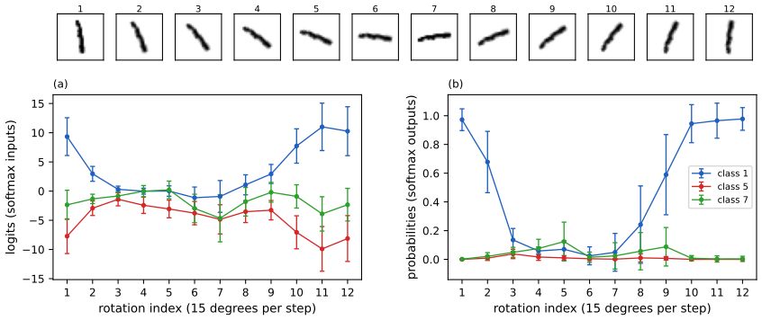
fig_17_2. Reproduces Murphy (2023), Figure 17.2 (our own network and rotated image). Download: PDF · SVGMC dropout is slow at test time (distillation, Section 17.3.10.3, removes the cost) and, more fundamentally, does not give proper uncertainty: although it is a variational method (Gal and Ghahramani), the approximating family is a mixture of point masses at zero and at the trained weight, which does not converge to the true posterior as \(N\to\infty\) because the dropout rate stays fixed (Osband 2016); the pathology is repaired if the rate is optimised (Gal et al. 2017).
Filling the gap 17.4: why the dropout predictive variance does not shrink with the data pp. 651–652
The book states that the dropout posterior "will not converge to the true posterior (a delta function at the MLE) even as the training set size goes to infinity". Here is the computation for a linear model, which shows the mechanism.
Derivation
Dropout on a linear model. Let \(f(\bm x;\bm w,\bm m)=\sum_im_iw_ix_i/(1-p)\) with independent masks \(m_i\sim\mathrm{Bernoulli}(1-p)\) (inverted dropout, so \(\E_m f=\bm w^\T\bm x\)). Over the masks, for fixed \(\bm w\) and \(\bm x\), \[ \var_m f=\sum_iw_i^2x_i^2\,\frac{p}{1-p}, \] since \(\var(m_i)=p(1-p)\). This is positive for every \(\bm w\) with a non-zero entry that meets a non-zero input and does not depend on \(N\).
The trained weights converge to a constant. Dropout least squares minimises \[ \E_m\|\bm y-\bm X(\bm m\odot\bm w)/(1-p)\|^2=\|\bm y-\bm X\bm w\|^2+\tfrac p{1-p}\sum_iw_i^2\|\bm X_{:i}\|^2 \], a ridge-type objective with solution \[ \hat{\bm w}=(\bm X^\T\bm X+\tfrac p{1-p}\diag(\bm X^\T\bm X))^{-1}\bm X^\T\bm y \]. Dividing numerator and denominator by \(N\) and applying the law of large numbers, \[ \hat{\bm w}\to(\bm\Sigma+\tfrac p{1-p}\diag\bm\Sigma)^{-1}\bm\Sigma\bm w^\star \] with \(\bm\Sigma=\E\bm x\bm x^\T\): a fixed vector with non-zero entries. So the MC dropout predictive variance converges to the positive constant \(\tfrac p{1-p}\sum_i\hat w_i^2x_i^2\) (in the limit it is also biased: the limit differs from \(\bm w^\star\)).
The exact posterior concentrates. With prior \(\N(\bm 0,\tau^2\bm I)\) and noise \(\sigma^2\), the posterior predictive variance of the function value is \[ \bm x^\T(\bm X^\T\bm X/\sigma^2+\bm I/\tau^2)^{-1}\bm x\le\sigma^2\bm x^\T(\bm X^\T\bm X)^{-1}\bm x=O(1/N)\to0 \]. The dropout "posterior" is a mixture of \(2^D\) point masses on the sub-vectors of \(\hat{\bm w}\): it assigns zero density to the neighbourhood of \(\bm w^\star\) in the full space, and its KL divergence to any continuous prior is infinite, so it is not a variational approximation in the sense of Chapter 10 unless the prior is also discrete (Hron et al. 2018). Figure 17.S4 shows the two behaviours; the bootstrap ensemble, like the exact posterior, shrinks as \(1/\sqrt N\).
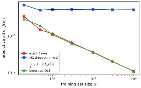
fig_17_S4. Download: PDF · SVG17.3.2 Laplace approximation
pp. 652–653, (17.14)–(17.16) The Laplace approximation (Section 7.4.3) is a Gaussian centred at the MAP estimate \(\th^\star\) whose precision is the Hessian of the negative log joint there. It can be applied to a pretrained network, but the Hessian is expensive and, because the loss is not convex, may be indefinite. With \(f(\bm x_n,\th)\in\R^C\), the residual \(\bm r(y;f)=\nabla_f\log p(y\given f)\), the noise term \(\bm\Lambda(y;f)=-\nabla_f^2\log p(y\given f)\), the Jacobian \(\bm J_\th(\bm x)\) (\(C\times P\)) and the network Hessian \(\bm H_\th(\bm x)\) (\(C\times P\times P\)),
\[ \nabla_\th\log p(y\given f(\bm x,\th))=\bm J_\th(\bm x)^\T\bm r(y;f),\qquad \nabla_\th^2\log p(y\given f(\bm x,\th))=\bm H_\th(\bm x)^\T\bm r(y;f)-\bm J_\th(\bm x)^\T\bm\Lambda(y;f)\bm J_\th(\bm x). \tag{17.14, 17.15}\]Dropping the network-Hessian term gives the generalised Gauss–Newton (GGN) approximation, which is positive semi-definite, and for a Gaussian prior \(\N(\bm m_0,\bm S_0)\) the Laplace approximation is \[ p(\th\given\mathcal D)\approx\N(\th^\star,\bm\Sigma_{\rm GGN}) \] with
\[ \bm\Sigma_{\rm GGN}^{-1}=\sum_{n=1}^N\bm J_{\th^\star}(\bm x_n)^\T\bm\Lambda(y_n;f_n)\bm J_{\th^\star}(\bm x_n)+\bm S_0^{-1}. \tag{17.16}\]Inverting a \(P\times P\) matrix costs \(O(P^3)\), so a diagonal approximation (\(O(P)\)) or a Kronecker-factored one (KFAC; Ritter et al. 2018) is used. The limits of the method: it is local (it knows only the curvature at the mode, so it can be too narrow or too broad, and a poor mode ruins it), and the curvature is used only after training, not while optimising; variational inference (next section) can be more accurate for similar cost.
Filling the gap 17.5: (17.14)–(17.16), positive definiteness of the GGN, and the linearised predictive (17.26)–(17.28) pp. 652–653, 661–662
The book quotes the gradient and Hessian, says the GGN is positive definite, and later (Section 17.3.10.1) that the linearised model gives a better predictive. All three follow from the chain rule and one observation.
Derivation
(17.14) and (17.15). Write \(\ell(\th)=\log p(y\given f(\bm x,\th))\). Chain rule: \[ \partial_{\theta_i}\ell=\sum_c(\partial_{f_c}\ell)(\partial_{\theta_i}f_c) \], so \(\nabla_\th\ell=\bm J^\T\bm r\). Differentiating again, \[ \partial_{\theta_i\theta_j}\ell=\sum_c\partial_{f_c}\ell\,\partial_{\theta_i\theta_j}f_c+\sum_{c,d}\partial_{f_cf_d}\ell\,\partial_{\theta_i}f_c\,\partial_{\theta_j}f_d \], that is \(\bm H^\T\bm r-\bm J^\T\bm\Lambda\bm J\) with \(\bm\Lambda=-\nabla_f^2\ell\). The first term is the part of the curvature that comes from the network's own non-linearity; it multiplies the residual and has no sign.
Positive semi-definiteness. If \(\ell\) is concave in \(f\) then \(\bm\Lambda\succeq0\), hence \(\bm J^\T\bm\Lambda\bm J\succeq0\) and \(\bm\Sigma_{\rm GGN}^{-1}\succ0\) (the prior adds \(\bm S_0^{-1}\succ0\)). Concavity holds for the usual likelihoods: Gaussian (\(\bm\Lambda=\sigma^{-2}\bm I\)), Bernoulli with logit \(f\) (\(\Lambda=\sigma(f)(1-\sigma(f))\)), categorical with logits (\(\bm\Lambda=\diag(\bm p)-\bm p\bm p^\T\), the covariance of the one-hot label) and generally every exponential family with the canonical link, for which \(\bm\Lambda\) is the covariance of the sufficient statistic. The full Hessian \(\sum_n(\bm H_n^\T\bm r_n)\) can make the sum indefinite at a point that is a saddle or a poor local minimum.
GGN = Fisher. For those likelihoods \(\E_{y\sim p(y\given f)}[\bm r\bm r^\T]=\bm\Lambda\), so \(\bm J^\T\bm\Lambda\bm J\) is the expected outer product of the score \(\nabla_\th\ell\): the GGN is the Fisher information matrix of the network, the matrix of natural-gradient methods (Chapter 6; Section 6.4).
Linearised model. Let \[ f_{\rm lin}(\bm x,\th)=f(\bm x,\th^\star)+\bm J(\bm x)(\th-\th^\star) \] (17.26). With a Gaussian likelihood and prior \(\N(\bm m_0,\bm S_0)\) the posterior of this model is Gaussian with precision \(\bm S_0^{-1}+\sum_n\bm J_n^\T\bm J_n/\sigma^2\), which is (17.16) with \(\bm\Lambda=\sigma^{-2}\bm I\). Its mean is \(\th^\star\): the gradient of the linearised log posterior at \(\th^\star\) equals that of the true one, because \(f_{\rm lin}\) and \(f\) agree to first order there, and the latter vanishes at the MAP. So the GGN Laplace approximation is exactly the posterior of the linearised model (Immer et al. 2021). Pushing a Gaussian through the linear map \(\th\mapsto f_{\rm lin}\) gives \[ p(\bm z\given\bm x,\mathcal D)=\N(\bm f(\bm x,\th^\star),\bm J(\bm x)\bm\Sigma\bm J(\bm x)^\T) \], (17.28) with the Jacobian written \(C\times P\) (the book's (17.28) writes \(\bm J^\T\bm\Sigma\bm J\) because there \(\bm J\) is \(P\times C\)). Sampling instead from the Gaussian and passing the samples through the nonlinear network (17.25) can put mass where the network is far from linear in \(\th\) and gives worse predictions; the linearised predictive avoids this. All statements were confirmed on a small network: the full Hessian differs from the GGN by the residual term and can have negative eigenvalues, and the posterior of the linearised model matches (17.16).
See also: the Laplace approximation of a Bayesian network, with its evidence, in Bayesian and Probabilistic ML, Section 5.7.1; the natural gradient and the Fisher matrix in Chapter 6, Section 6.4.
17.3.3 Variational inference
pp. 653–654, Figure 17.3 Fixed-form variational inference (Section 10.2) chooses \(q_\psi(\th)=\N(\th\given\bm\mu,\bm\Sigma)\) and minimises \(\KL(q\,\|\,p(\cdot\given\mathcal D))\); with the reparameterisation trick the ELBO gradient has low variance, but the minimiser differs from the Laplace approximation (it is mode-seeking over a region, not a local curvature). Hinton and Camp (1993) introduced variational methods for networks; Graves (2011) used a diagonal Gaussian (every weight gets its own mean and variance, Figure 17.3); Blundell et al. (2015) added the reparameterisation trick (Bayes by backprop, an instance of the SVI algorithm of Chapter 10 with a Gaussian prior and posterior). Extensions: the local reparameterisation trick (Kingma et al. 2015), VOGN (a noisy natural-gradient method; Khan et al. 2018, Osawa et al. 2019), low-rank plus diagonal posteriors (Mishkin et al. 2018) and a rank-one plus diagonal one (Tran et al. 2020).
Filling the gap 17.6: the Gaussian KL term, and why local reparameterisation reduces the variance p. 654
The book names the local reparameterisation trick without saying why it helps. Here is the variance computation, with the closed-form KL used by Bayes by backprop.
Derivation
The ELBO. With the fully factorised posterior \(q(\th)=\prod_i\N(\theta_i\given\mu_i,\sigma_i^2)\) and the prior \(\N(0,s^2)\) on every weight, \[ \ELBO(\bm\mu,\bm\sigma)=\E_q\Big[\sum_{n}\log p(y_n\given\bm x_n,\th)\Big]-\sum_i\Big(\log\frac{s}{\sigma_i}+\frac{\sigma_i^2+\mu_i^2}{2s^2}-\frac12\Big). \] The KL term is the standard Gaussian-to-Gaussian formula, summed over weights (the prior and the posterior are products). The reparameterisation \(\theta_i=\mu_i+\sigma_i\epsilon_i\) with \(\epsilon_i\sim\N(0,1)\) lets the gradient pass inside the expectation (Section 10.2.1): \(\nabla_{\bm\mu}\E_q[g]=\E_\epsilon[\nabla_\th g]\), \[ \nabla_{\sigma_i}\E_q[g]=\E_\epsilon[\epsilon_i\partial_{\theta_i}g] \].
Why sharing one weight sample across a minibatch is costly. For one layer \(\bm a_b=\bm W^\T\bm z_b\) with minibatch \(b=1,\dots,B\), the estimate of the data term is \(\frac1B\sum_bg_b(\bm W)\) with a single draw \(\bm W\) shared by all examples. Its variance is \[ \var\Big[\frac1B\sum_bg_b\Big]=\frac1{B^2}\sum_b\var g_b+\frac1{B^2}\sum_{b\ne b'}\cov(g_b,g_{b'}). \] The first term is \(O(1/B)\). The second is \(O(1)\) (it has \(B(B-1)\) terms and a \(1/B^2\) factor), so it does not vanish as the minibatch grows: the examples all feel the same weight noise, and their gradients are positively correlated.
Local reparameterisation. If \(W_{ij}\sim\N(\mu_{ij},\sigma_{ij}^2)\) independently and \(\bm z\) is fixed, the pre-activation \(a_j=\sum_iW_{ij}z_i\) is Gaussian with \[ \E a_j=\sum_i\mu_{ij}z_i,\qquad\var a_j=\sum_i\sigma_{ij}^2z_i^2, \] and, for fixed \(\bm z_b\), the activations of different examples are marginally of this form. Drawing \(a_{bj}=\gamma_{bj}+\delta_{bj}\xi_{bj}\) with \(\gamma_{bj}=\sum_i\mu_{ij}z_{bi}\), \(\delta_{bj}^2=\sum_i\sigma_{ij}^2z_{bi}^2\) and an independent \(\xi_{bj}\sim\N(0,1)\) for each example gives the same marginal law for each \(a_b\) but removes the covariance between examples, because the noises \(\xi_{bj}\) are independent. The estimator is then unbiased for the same expectation (the objective only depends on the marginals of the activations of each single example) with variance \(O(1/B)\). It is also cheaper: it needs \(B\times n_{\rm out}\) random numbers instead of \(n_{\rm in}\times n_{\rm out}\). A numerical experiment with a Bayesian linear layer (32 examples, six inputs) confirmed that the two estimators have the same mean for the gradients with respect to the mean and to the standard deviation, and that the shared-sample estimator of the latter has about twelve times the variance of the local one.
See also: the SVI algorithm and the reparameterisation estimator: Chapter 10 notes, Section 10.2.1; online variational inference is Section 17.5.4 below.
17.3.4 Expectation propagation
p. 654 Expectation propagation (EP) locally minimises \(\KL(p\,\|\,q)\) rather than \(\KL(q\,\|\,p)\) (Section 10.7; notes). Assumed density filtering (ADF, Section 8.6) is the first pass of EP; Hernández-Lobato and Adams (2015) applied it to networks as probabilistic backpropagation (PBP), approximating every weight by a Gaussian factor (Figure 17.3). The updates are derived in Filling the gap 17.26 and the algorithm is Section 17.5.3.
17.3.5 Last layer methods
pp. 654–655, (17.17) The simplest approximation is Bayesian only about the last layer and uses MAP estimates elsewhere: the neural-linear model (Riquelme et al. 2018). With logits \(\bm z=\bm w_L^\T\bm\phi(\bm x;\th)\) the model is a Bayesian generalised linear model in the features \(\bm\phi\); Laplace (Section 15.3.5) gives \(p(\bm w_L\given\mathcal D)=\N(\bm\mu_L,\bm\Sigma_L)\) and
\[ p(\bm z\given\bm x,\mathcal D)=\N\big(\bm z\given\bm\mu_L\bm\phi(\bm x),\ \bm\phi(\bm x)\bm\Sigma_L\bm\phi(\bm x)^\T\big), \tag{17.17}\]which a softmax or a probit then turns into class probabilities (Section 15.3.6). Kristiadi et al. (2020) show that this reduces over-confidence away from the data; the price is that uncertainty in the feature extractor, where most parameters live, is ignored.
Filling the gap 17.7: the Gaussian-logit predictive (17.17) and the probit integral (17.52) pp. 655, 676
The book quotes (17.17) and the integral (17.52) of a Gaussian against the normal CDF without proof. Both are short.
Derivation
(17.17). If \(\bm w\sim\N(\bm\mu,\bm\Sigma)\) then each logit \(z_c=\bm w_c^\T\bm\phi\) is a linear function of a Gaussian vector for fixed \(\bm\phi\), hence Gaussian with mean \(\bm\mu_c^\T\bm\phi\) and covariance \(\bm\phi^\T\bm\Sigma\bm\phi\) (the covariance of a linear image). The variance grows with \(\|\bm\phi\|\), which is what makes the neural-linear model less confident for inputs whose features are far from the training features (when the features themselves do not collapse, see Section 17.3.6).
(17.52). Let \(U\sim\N(0,1)\) be independent of \(\eta\sim\N(\mu,\sigma^2)\). Then \(\Phi(y\eta)=\Pr(U\le y\eta\given\eta)\), so \[ \int\Phi(y\eta)\,\N(\eta\given\mu,\sigma^2)\d\eta=\Pr(U-y\eta\le0). \] Now \(U-y\eta\) is Gaussian with mean \(-y\mu\) and variance \(1+y^2\sigma^2=1+\sigma^2\) (for \(y=\pm1\)), so the probability is \(\Phi\big(y\mu/\sqrt{1+\sigma^2}\big)\). (The book writes \(\sqrt{1+\sigma}\) and \(\N(h\given\mu,\sigma)\); \(\sigma\) there is a variance and \(h\) should read \(\eta\).) For the logistic output, \(\sigma(a)\approx\Phi(\sqrt{\pi/8}\,a)\) (the two sigmoids have equal slope at the origin), so \[ \int\sigma(\eta)\N(\eta\given\mu,v)\d\eta\approx\sigma\big(\mu/\sqrt{1+\pi v/8}\big) \], the probit approximation of Section 15.3.6. The numbers confirm the integral to quadrature precision, and the approximation to about 0.01 in probability.
17.3.6 SNGP
p. 655 A DNN can be a feature extractor for a Gaussian process (deep kernel learning, Section 18.6.6), but training for classification accuracy alone does not stop the features from collapsing far-apart inputs onto each other: there is no loss penalty for moving two inputs close together, if they are on the same side of the boundary, so an OOD input can land next to a training point. The spectrally normalised Gaussian process (SNGP; Liu et al. 2020, 2022) makes the extractor distance preserving by spectral normalisation of the weights (a bound on the Lipschitz constant) and puts a GP output layer, implemented with random features, on top.
Filling the gap 17.8: random Fourier features, and why spectral normalisation preserves distances p. 655
The book describes SNGP in prose. Two facts make it work and both have short proofs.
Derivation
Random features for the RBF kernel. Let \(k(\bm h,\bm h')=\exp(-\|\bm h-\bm h'\|^2/(2\ell^2))\). Draw \(\bm\omega\sim\N(\bm 0,\ell^{-2}\bm I)\) and \(b\sim\mathrm{Uniform}(0,2\pi)\) independently and set \(\varphi(\bm h)=\sqrt2\cos(\bm\omega^\T\bm h+b)\). By the product-to-sum identity, \[ \varphi(\bm h)\varphi(\bm h')=\cos(\bm\omega^\T(\bm h-\bm h'))+\cos(\bm\omega^\T(\bm h+\bm h')+2b) \]. The second term has mean zero over \(b\); the first has mean \[ \E\cos(\bm\omega^\T\bm\delta)=\exp(-\|\bm\delta\|^2/(2\ell^2)) \], the characteristic function of the Gaussian, with \(\bm\delta=\bm h-\bm h'\). So \(\E[\varphi(\bm h)\varphi(\bm h')]=k(\bm h,\bm h')\). With \(D\) independent copies and \(\bm\phi=\sqrt{2/D}\,\cos(\bm R^\T\bm h+\bm b)\) the estimate \(\bm\phi^\T\bm\phi'\) of \(k\) has variance \(\frac1D\big(1+\tfrac12k^4-k^2\big)\le\frac1D\), where the middle term comes from \[ \E\cos^2(\bm\omega^\T\bm\delta)=\tfrac12(1+\E\cos(2\bm\omega^\T\bm\delta))=\tfrac12(1+k^4) \]. A Bayesian linear model \(z=\bm\beta^\T\bm\phi(\bm h)\) with prior \(\bm\beta\sim\N(\bm 0,\bm I)\) is therefore (as \(D\to\infty\)) a GP with kernel \(k\) in the feature space \(\bm h\); its posterior is the last-layer posterior (17.17). The predictive variance of the logit is \(\bm\phi^\T\bm\Sigma\bm\phi\to k(\bm h,\bm h)=1\) minus what the training points explain, and the explained part is \(k(\bm h,\bm h_n)\to0\) when \(\bm h\) is far from every training feature. Distance awareness therefore holds if distances between features reflect distances between inputs.
Spectral normalisation. Let \(g(\bm x)=\phi_L(\bm W_L\cdots\phi_1(\bm W_1\bm x))\) with each \(\phi_\ell\) 1-Lipschitz (ReLU, tanh). Since \(\|\bm W\bm u-\bm W\bm v\|\le\|\bm W\|_2\|\bm u-\bm v\|\) with \(\|\bm W\|_2\) the largest singular value, \[ \|g(\bm x)-g(\bm x')\|\le\prod_\ell\|\bm W_\ell\|_2\,\|\bm x-\bm x'\| \]; rescaling each \(\bm W_\ell\) to \(\|\bm W_\ell\|_2\le c\) bounds the Lipschitz constant by \(c^L\). That is an upper bound: it prevents expansion but not collapse. The lower bound comes from the residual form \(\bm h_{\ell+1}=\bm h_\ell+r_\ell(\bm h_\ell)\) with \(r_\ell\) \(c\)-Lipschitz, \(c<1\): by the reverse triangle inequality \[ \|\bm h_{\ell+1}-\bm h'_{\ell+1}\|\ge\|\bm h_\ell-\bm h'_\ell\|-\|r_\ell(\bm h_\ell)-r_\ell(\bm h'_\ell)\|\ge(1-c)\|\bm h_\ell-\bm h'_\ell\| \], so \[ (1-c)^L\|\bm x-\bm x'\|\le\|\bm h_L(\bm x)-\bm h_L(\bm x')\|\le(1+c)^L\|\bm x-\bm x'\| \]: the extractor is bi-Lipschitz, and distant inputs stay distant. A numerical experiment with random residual blocks of spectral norm 0.9 confirmed both bounds and the random-feature variance.
17.3.7 MCMC methods
pp. 655–656, Figure 17.4 Neal (1996) used Hamiltonian Monte Carlo (Section 12.5; notes) for networks, and it is generally regarded as the gold standard since it makes no assumption on the shape of the posterior; recent work scales it up (Izmailov et al. 2021; Cobb and Jalaian 2021). Figure 17.4 fits a two-hidden-layer MLP to 50 two-moons points with HMC and plots the posterior mean and standard deviation of \(p(y=1\given\bm x)\): the uncertainty grows away from the data. HMC needs the whole training set at every step; stochastic-gradient MCMC (Section 12.7.1) uses minibatches.
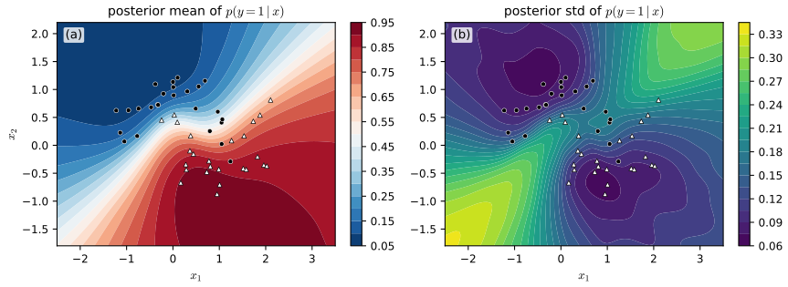
fig_17_4, hmc_batched. Reproduces Murphy (2023), Figure 17.4 (our own network and sampler). Download: PDF · SVGFilling the gap 17.9: the posterior of a network has at least \(2^HH!\) copies of every mode pp. 655–656, 659
The book remarks that "modern deep neural networks have highly multi-modal posteriors". Part of the multimodality is exact, and it is easy to count.
Derivation
Symmetries. Take a hidden layer of \(H\) units with an odd activation (tanh) and weights \((\bm W_{\rm in}\in\R^{H\times n},\bm b,\bm W_{\rm out}\in\R^{m\times H})\). (i) Permuting the hidden units (the rows of \((\bm W_{\rm in},\bm b)\) and the columns of \(\bm W_{\rm out}\) in the same way) leaves \(f(\bm x;\th)\) unchanged, because the layer output is a sum over units. (ii) Negating unit \(j\) (its row of \(\bm W_{\rm in}\), its bias and its column of \(\bm W_{\rm out}\)) leaves \(f\) unchanged, because \(\tanh(-a)=-\tanh(a)\). Together they form a group of size \(2^HH!\) acting on the weight space; for generic weights its images are distinct points. For ReLU units sign flips are not symmetries, but permutations and the rescalings \[ (\bm w_{\rm in},b,\bm w_{\rm out})\to(c\bm w_{\rm in},cb,\bm w_{\rm out}/c) \] are.
Consequence for the posterior. The i.i.d. symmetric Gaussian prior \(p(\th)\) is invariant under permutation and sign change of coordinates, and the likelihood \(p(\mathcal D\given\th)=\prod_np(y_n\given f(\bm x_n;\th))\) depends on \(\th\) only through \(f\). Hence the posterior is invariant, and each mode has \(2^HH!\) images (384 for \(H=4\), about \(10^{16}\) for \(H=16\)), related by an isometry. Two things follow. First, the posterior mean of the weights is meaningless (the average over the sign-flip orbit of a unit's outgoing weight is zero) and parameter-space summaries of a chain are not interpretable; only function-space quantities such as \(p(y\given\bm x,\mathcal D)\) are. Second, a Markov chain that stays inside one copy of a mode still explores the posterior over functions near that mode, so the quantities in Figures 17.4 and 17.15 are well defined; what is not explored by a local sampler is the set of functionally distinct modes (Section 17.3.9 below) separated by high-loss barriers. A numerical experiment confirmed (i) and (ii) for a random network and the counts above.
See also: hierarchical models in Section 17.6 break these symmetries between tasks because all tasks share the global weights.
17.3.8 Methods based on the SGD trajectory
pp. 656–657, Figure 17.5 Under some assumptions the iterates of SGD at a fixed learning rate are samples from a Gaussian around a local mode (Mandt et al. 2017; Chaudhari and Soatto 2018; Smith and Le 2018), so SGD can generate approximate posterior samples, much as SG-MCMC does except that no noise is added and the step size is not decayed. Izmailov et al. (2018) noted that these iterates lie on the periphery of a region of good solutions (Figure 17.5) and averaged iterates taken once per epoch, \(\bar\th=\frac1S\sum_s\th_s\): stochastic weight averaging (SWA), which tends to find broader minima. SWA differs from Polyak–Ruppert averaging (learning rate decaying to zero, an exponential moving average, aimed at variance reduction) and relates to snapshot ensembles and fast geometric ensembles, which average predictions over cyclically collected iterates. Maddox et al. (2019) fit a Gaussian to the iterates, SWAG: the mean is the SWA solution and the covariance \[ \bm\Sigma=\tfrac12(\bm\Sigma_{\rm diag}+\bm\Sigma_{\rm lr}) \] averages a diagonal part \(\diag(\overline{\th^2}-\bar\th^2)\) and a low-rank part from the last \(K\) deviations \(\bm\Delta_i=\th_i-\bar\th_i\) (the running mean), \(\bm\Sigma_{\rm lr}=\frac1K\bm\Delta\bm\Delta^\T\) as printed (the original uses \(K-1\)).
Filling the gap 17.10: the stationary law of constant-step SGD and why averaging helps pp. 656–657
The book cites the claim and its corollary (the SWA point is better than the iterates). For a quadratic loss both are exact computations.
Derivation
The stationary distribution. Let \(L(\th)=\tfrac12\th^\T\bm A\th\) and let the stochastic gradient be \(\bm A\th+\bm\xi\) with mean-zero independent noise of covariance \(\bm B\). With step \(\varepsilon\), \[ \th_{t+1}=(\bm I-\varepsilon\bm A)\th_t-\varepsilon\bm\xi_t \] is a stable linear recursion if \(\|\bm I-\varepsilon\bm A\|_2<1\), and its stationary covariance \(\bm\Sigma\) solves \[ \bm\Sigma=(\bm I-\varepsilon\bm A)\bm\Sigma(\bm I-\varepsilon\bm A)+\varepsilon^2\bm B. \] If \(\bm A=\diag(a_i)\) and \(\bm B=\diag(b_i^2)\), then \[ \Sigma_{ii}=\varepsilon^2b_i^2/(1-(1-\varepsilon a_i)^2)=\varepsilon b_i^2/(a_i(2-\varepsilon a_i)) \]. For small \(\varepsilon\) this is the continuous Lyapunov equation \(\bm A\bm\Sigma+\bm\Sigma\bm A=\varepsilon\bm B\). Two cases: if the noise is isotropic, \(\bm B=b^2\bm I\), then \(\bm\Sigma=\tfrac{\varepsilon b^2}2\bm A^{-1}\), the Gaussian \(\propto\exp(-L(\th)/T)\) with temperature \(T=\varepsilon b^2/2\), the posterior of Langevin dynamics (Filling the gap 12.15); if the noise covariance is proportional to the curvature, \(\bm B=c\bm A\) (the empirical Fisher is close to the Hessian near a minimum), then \(\bm\Sigma=\tfrac{\varepsilon c}2\bm I\). Either way the iterates form a Gaussian cloud around the minimum, not a point, with a width set by \(\varepsilon\) (Figure 17.S2a). The agreement of the exact discrete formula with simulation was confirmed.
Why the average is better. In \(D\) dimensions a single iterate satisfies \(\E\|\th_s\|^2=\Tr\bm\Sigma\), and the squared radius concentrates (it is a sum of \(D\) independent terms), so the iterates sit on a shell of radius \(\sqrt{\Tr\bm\Sigma}\) around the minimum, as in Figure 17.5. For the average of \(K\) iterates taken every \(\tau\) steps, coordinate \(i\) is an AR(1) process with lag-\(\tau\) correlation \(\rho_i=(1-\varepsilon a_i)^\tau\) (in the diagonal case), and for large \(K\) \[ \E\|\bar\th_K\|^2\simeq\frac1K\sum_i\Sigma_{ii}\,\frac{1+\rho_i}{1-\rho_i}, \] which is \(\Tr\bm\Sigma/K\) when the samples are essentially independent (\(\rho_i\approx0\)). The loss of the average is \[ \E L(\bar\th_K)=\tfrac12\sum_ia_i\E\bar\theta_{K,i}^2\approx\E L(\th_s)/K \]: averaging \(K\) spaced iterates reduces the excess loss by about a factor \(K\), without extra gradient evaluations (Figure 17.S2b, \(D=100\)). SWA is thus a cheap approximation of the posterior mean (the centre of the Gaussian), and SWAG adds the spread. For a non-quadratic loss the argument is local; the conclusion that the average lies in a flatter region is the point of Section 17.4.1.
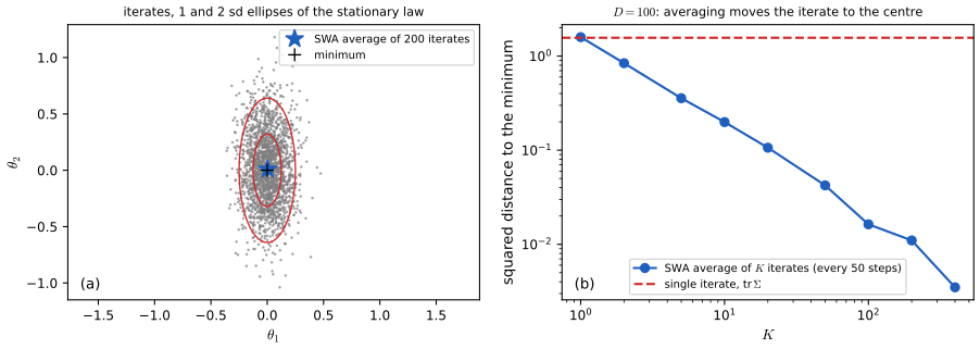
fig_17_S2, sgd_quadratic. Download: PDF · SVG17.3.9 Deep ensembles
pp. 657–661, (17.18)–(17.23), Figures 17.6–17.8 Most approximations are local to one mode, but the posterior of a deep network is highly multimodal and different modes encode different functions, while functions near one mode tend to agree. A local approximation therefore underestimates uncertainty. The simplest alternative is an equally weighted mixture of point masses at \(M\) independently trained MAP estimates,
\[ p(\th\given\mathcal D)\approx\frac1M\sum_{m=1}^M\delta(\th-\hat\th_m) \tag{17.18}\](Lakshminarayanan et al. 2017; Fort et al. 2019), the deep ensemble (Figure 17.6 sketches subspace methods around one mode against ensembles over distinct modes). The members may differ in seed, hyperparameters, architecture, or with an explicit repulsive term to force functional diversity.
17.3.9.1 Multi-SWAG
p. 658, (17.19) Fitting a SWAG Gaussian around each of the \(M\) modes gives the mixture \[ p(\th\given\mathcal D)\approx\frac1M\sum_m\N(\th\given\hat\th_m,\bm\Sigma_m) \] (17.19) (MultiSWAG; Wilson and Izmailov 2020): it averages across basins like a deep ensemble and within each basin, and can produce any number \(S>M\) of samples.
17.3.9.2 Deep ensembles with random priors
pp. 658–659, (17.20), Figure 17.7 Members trained from different initialisations on the same data are often similar. Diversity can be added by bootstrapping the data, or by letting member \(i\) be the sum of a trainable network \(t_i\) and a fixed random prior network \(p_i\) scaled by \(\beta\ge0\), \(g_i(\bm x;\th_i)=t_i(\bm x;\th_i)+\beta\,p_i(\bm x)\) (17.20); \(t_i\) learns the residual between the data and the prior function (Osband et al. 2018). Larger \(\beta\) means more data-independent variation among members and a more diffuse posterior. Figure 17.7 shows members (left) and the ensemble for four values of \(\beta\) (right).
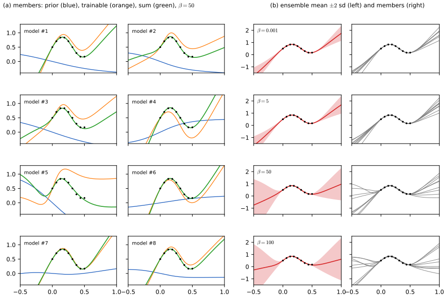
fig_17_7, random_prior_ensemble. Reproduces Murphy (2023), Figure 17.7 (our own data and networks; the scale of \(p_i\) is chosen so that \(\beta\) of order 100 matters). Download: PDF · SVGFilling the gap 17.11: random-prior ensembles are exact posterior samples for a linear model (randomize-then-optimise) pp. 658–659, (17.20)
The book presents (17.20) as a heuristic for diversity. For a linear model it is an exact sampler, which explains why \(\beta\) acts as the prior scale.
Derivation
Statement. Let \(\bm y=\bm\Phi\th+\bm\varepsilon\), \(\bm\varepsilon\sim\N(\bm 0,\sigma^2\bm I_N)\), prior \(\th\sim\N(\bm 0,\tau^2\bm I_P)\). Draw independently \(\th_0\sim\N(\bm 0,\tau^2\bm I)\) and \(\bm e\sim\N(\bm 0,\sigma^2\bm I_N)\) and let \[ \hat\th=\argmin_\th\ \frac1{\sigma^2}\|\bm y+\bm e-\bm\Phi\th\|^2+\frac1{\tau^2}\|\th-\th_0\|^2. \] Then \(\hat\th\sim\N(\bm m,\bm S)\), the exact posterior, with \(\bm S=\bm A^{-1}\), \(\bm A=\bm\Phi^\T\bm\Phi/\sigma^2+\bm I/\tau^2\), \(\bm m=\bm A^{-1}\bm\Phi^\T\bm y/\sigma^2\).
Proof. The objective is a quadratic with minimiser \[ \hat\th=\bm A^{-1}\big(\bm\Phi^\T(\bm y+\bm e)/\sigma^2+\th_0/\tau^2\big) \], a linear function of the independent Gaussians \(\bm e,\th_0\), hence Gaussian. Its mean is \(\bm A^{-1}\bm\Phi^\T\bm y/\sigma^2=\bm m\). Its covariance is \[ \bm A^{-1}\Big(\frac{\bm\Phi^\T(\sigma^2\bm I)\bm\Phi}{\sigma^4}+\frac{\tau^2\bm I}{\tau^4}\Big)\bm A^{-1}=\bm A^{-1}\Big(\frac{\bm\Phi^\T\bm\Phi}{\sigma^2}+\frac{\bm I}{\tau^2}\Big)\bm A^{-1}=\bm A^{-1}. \qquad\blacksquare \]
The random prior function. Write \(f(\bm x;\th)=\bm\phi(\bm x)^\T\th\), a random prior function \(p(\bm x)=\bm\phi(\bm x)^\T\th_0\) and a trainable part \(t(\bm x)=\bm\phi(\bm x)^\T\bm w\) with \(\bm w=\th-\th_0\). Then \(g=t+p=\bm\phi^\T\th\) and the penalty \(\|\th-\th_0\|^2/\tau^2=\|\bm w\|^2/\tau^2\) is an ordinary weight decay on the trainable part only, while the data term is the squared error of \(t+p\) to \(\bm y+\bm e\), i.e. \(t\) fits the residual \(\bm y+\bm e-p(\bm x_n)\). That is the random-prior ensemble of (17.20), with \(\beta\) absorbed into the scale \(\tau\) of the prior function (a larger \(\beta\) means a larger \(\tau\)). Two refinements: without the data-noise draw \(\bm e\) the covariance is \(\bm A^{-1}\bm I\bm A^{-1}/\tau^2\preceq\bm S\) (too small in the directions the data determine), and without \(\th_0\) it is \(\bm A^{-1}\bm\Phi^\T\bm\Phi\bm A^{-1}/\sigma^2\) (too small away from the data); Figure 17.S3 shows both failures. For a network the statement holds approximately in the linearised ("lazy") regime (He et al. 2020) and otherwise only as a heuristic. A simulation of the three variants matched the formulas.
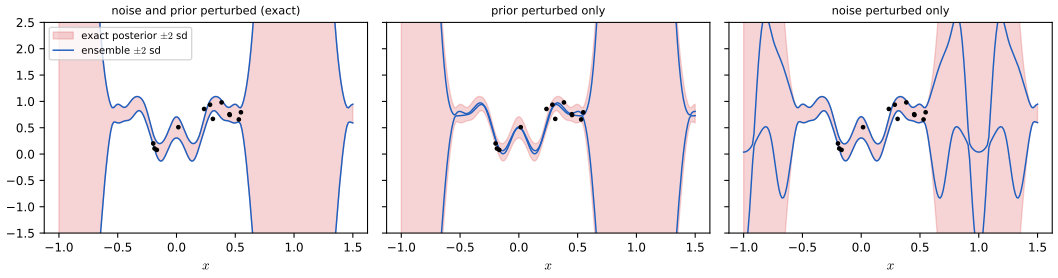
fig_17_S3, rto_samples. Download: PDF · SVG17.3.9.3 Deep ensembles as approximate Bayesian inference
p. 659 No inference scheme for a network is exact; they lie on a spectrum of how closely they approximate the true posterior predictive. Because point masses at different modes represent more functional diversity than samples from one basin, deep ensembles can approximate the Bayesian model average better than a single-basin method. The accuracy of any approximation \(q\) is governed by Result 17.1 applied to \(q\): the ensemble predictive is the mixture of its members, never worse in log loss than their average, with the epistemic term measuring their disagreement.
17.3.9.4 Deep ensembles vs classical ensembles
pp. 659–660 Bagging and random forests (Dietterich 2000) get diversity from resampled data or features, which is necessary when the base learner is a convex problem (a linear model or a shallow tree: the same data give the same solution). Deep ensembles train every member on the same data and features; the diversity comes from the initialisation, the SGD noise and the non-convexity. Diversity can also be enforced, provably improving performance (Theisen and Brewer 2022).
17.3.9.5 Deep ensembles vs mixtures of experts and stacking
p. 660, (17.21) A Bayesian model average weights the models by their posterior probabilities \(p(m\given\mathcal D)\propto p(\mathcal D\given m)p(m)\). In the large-sample limit the ratio of two marginal likelihoods behaves like \(e^{-N\Delta}\) with \(\Delta\) the difference of the KL divergences of the two models from the data-generating law, so the weights concentrate on one model; a deep ensemble keeps \(M\) equal weights, so BMA and ensembling differ, and ensembling can enlarge the expressive power of the predictive (Minka 2000; Oh et al. 2021). Making the weights depend on the input, \[ p(y\given\bm x,\mathcal D)=\sum_mw_m(\bm x)\,p(y\given\bm x,\th_m),\tag{17.21}\] gives a mixture of experts when \(w_m\ge0\), \(\sum_mw_m=1\); allowing any positive weights gives stacking (Wolpert 1992; Yao et al. 2018), whose weights are fitted on held-out data and are more robust to misspecification.
17.3.9.6 Batch ensemble
pp. 660–661, (17.22)–(17.23), Figure 17.8 An ensemble costs \(M\) times the memory and time. Batch ensemble (Wen et al. 2020) shares a "slow" weight matrix \(\bm W\) and gives member \(m\) a rank-one "fast" perturbation, \(\bm W_m=\bm W\odot\bm F_m\) with \(\bm F_m=\bm s_m\bm r_m^\T\). The layer output on example \(\bm x_n\) is
\[ \bm y_n^m=\phi\big(\bm W_m^\T\bm x_n\big)=\phi\big((\bm W\odot\bm s_m\bm r_m^\T)^\T\bm x_n\big)=\phi\big((\bm W^\T(\bm x_n\odot\bm s_m))\odot\bm r_m\big), \tag{17.22}\]and for a minibatch \(\bm X\), \(\bm Y_m=\phi(((\bm X\odot\bm S_m)\bm W)\odot\bm R_m)\) (17.23), with \(\bm S_m,\bm R_m\) the vectors replicated over the rows. Only \(2M\) vectors per layer are stored beyond \(\bm W\), and all members can be run in one batched matrix product.
Filling the gap 17.12: the batch-ensemble identity (17.22) and the parameter count pp. 660–661
The book states the identity and the saving without proof.
Derivation
Let \(\bm W\in\R^{n_{\rm in}\times n_{\rm out}}\), \(\bm s\in\R^{n_{\rm in}}\), \(\bm r\in\R^{n_{\rm out}}\). The \((i,j)\) entry of \(\bm W\odot\bm s\bm r^\T\) is \(W_{ij}s_ir_j\), so \[ \big[(\bm W\odot\bm s\bm r^\T)^\T\bm x\big]_j=\sum_iW_{ij}s_ir_jx_i=r_j\sum_iW_{ij}(s_ix_i)=\big[(\bm W^\T(\bm x\odot\bm s))\odot\bm r\big]_j, \] which is (17.22): scale the input elementwise by \(\bm s\), multiply by the shared matrix, then scale the output elementwise by \(\bm r\). The matrix-vector product with the shared \(\bm W\) is the only quadratic cost, and it can be done for all members as one product on the stacked inputs \(\bm X\odot\bm S_m\), which gives (17.23). Parameters: \(n_{\rm in}n_{\rm out}+M(n_{\rm in}+n_{\rm out})\) per layer against \(Mn_{\rm in}n_{\rm out}\) for \(M\) separate networks, a saving by a factor of about \(M\) when the layer is wide. The members are not independent networks: they are rank-one rescalings of one matrix, which limits their diversity (Wen et al. 2020 combine the method with MC dropout for this reason). A numerical experiment of (17.22), (17.23) and the counts agreed.
17.3.10 Approximating the posterior predictive distribution
p. 661, (17.24)–(17.25) Given \(q(\th)\approx p(\th\given\mathcal D)\) the predictive is \(\int q(\th)p(y\given\bm x,\th)\d\th\) (17.24), approximated by Monte Carlo \(\frac1S\sum_sp(y\given f(\bm x,\th_s))\) with \(\th_s\sim q\) (17.25).
17.3.10.1 A linearized approximation
pp. 661–662, (17.26)–(17.28) Samples of \(\th\) from a Gaussian centred at the MAP can lie where \(f(\bm x;\th)\) is far from its linearisation, giving poor predictions (Immer et al. 2021). Replacing \(f\) by \[ f^{\th^\star}_{\rm lin}(\bm x,\th)=f(\bm x,\th^\star)+\bm J(\bm x)(\th-\th^\star) \] (17.26) gives a generalised linear model whose Gaussian predictive over logits is \(\N(f(\bm x,\bm\mu),\bm J\bm\Sigma\bm J^\T)\) (17.28), and the predictive (17.27) uses samples through the linear map. The class probabilities then follow from a probit approximation or the Laplace bridge. The derivation is in Filling the gap 17.5.
17.3.10.2 The Laplace bridge approximation
pp. 662–664, (17.29)–(17.31), Figure 17.9 A point estimate of the class probabilities does not say how sure we are of them. The Laplace bridge (Hobbhahn et al. 2022) turns a Gaussian approximation of the logits \(\N(\bm z\given\bm m,\bm V)\) (from (17.28) or (17.17)) into a Dirichlet over the probabilities, as a post-processing step:
\[ \alpha_i=\frac1{V_{ii}}\Big(1-\frac2C+\frac{e^{m_i}}{C^2}\sum_{j=1}^Ce^{-m_j}\Big), \tag{17.29}\]with \(C\) the number of classes, and \(p_c=\alpha_c/\alpha_0\). The derivation assumes the logits sum to zero (a Dirichlet has one degree of freedom fewer), so first condition on \(\bm 1^\T\bm z=0\):
\[ p(\bm z\given\bm x,\mathcal D)=\N\Big(\bm z\ \Big|\ \bm m-\frac{\bm V\bm1\bm1^\T\bm m}{\bm1^\T\bm V\bm1},\ \bm V-\frac{\bm V\bm1\bm1^\T\bm V}{\bm1^\T\bm V\bm1}\Big)=\N(\bm z\given\bm m',\bm V'). \tag{17.30}\]To avoid sparse \(\bm\alpha\), the bridge also rescales \(\bm m''=\bm m'/\sqrt c\), \(\bm V''=\bm V'/c\) with \(c=(\sum_iV'_{ii})/\sqrt{C/2}\). Since Dirichlet marginals are Beta distributions, the marginal over the probability of the top class is \(\mathrm{Beta}(\tilde\alpha_1,\alpha_0-\tilde\alpha_1)\) (17.31) (labels sorted by \(\tilde\alpha\)), and similarly for the others; returning all labels whose marginals overlap that of the top label gives an adaptive prediction set, in the spirit of conformal prediction (Section 14.3.1) but Bayesian and per-instance. Figure 17.9 (ImageNet with a pretrained network) is not reproduced; the bridge is examined on Gaussian logits in Figure 17.S1, where it is accurate only for large concentrations and when the logit variances have the pattern of a Dirichlet.
Filling the gap 17.13: where (17.29) and (17.30) come from pp. 662–663
The book quotes the formula from Hobbhahn et al. (2022). It is the inverse of the Laplace approximation of a Dirichlet in the softmax basis, read off its diagonal.
Derivation
A Dirichlet is a normalised vector of gammas. If \(g_k\sim\mathrm{Gamma}(\alpha_k,1)\) independently, \(\bm\pi=\bm g/\sum_kg_k\sim\Dir(\bm\alpha)\). With \(y_k=\log g_k\) the logits \(z_k=y_k-\bar y\) (\(\bar y\) the mean) are the zero-sum logits of \(\bm\pi\), up to a constant.
Laplace approximation of one \(y_k\). The density of \(y_k\) is proportional to \(\exp(\alpha_ky-e^y)\) (the Jacobian \(e^y\) of \(g=e^y\) multiplies \(g^{\alpha_k-1}\)). Its mode is \(y=\log\alpha_k\), and the second derivative of the log density is \(-e^y=-\alpha_k\) there, so \(y_k\approx\N(\log\alpha_k,1/\alpha_k)\), independently over \(k\). Centring with \(\bm P=\bm I-\bm1\bm1^\T/C\): \[ \bm z\approx\N\big(\log\bm\alpha-\overline{\log\alpha}\,\bm1,\ \bm P\diag(1/\bm\alpha)\bm P\big), \] that is \(\mu_k=\log\alpha_k-c\) with \(c=\frac1C\sum_l\log\alpha_l\), and \[ \Sigma_{kk}=\frac1{\alpha_k}\Big(1-\frac2C\Big)+\frac1{C^2}\sum_u\frac1{\alpha_u}, \] using \((\bm P\bm D\bm P)_{kk}=D_k-\frac2CD_k+\frac1{C^2}\sum_uD_u\) for diagonal \(\bm D=\diag(1/\bm\alpha)\). This is the Laplace approximation of a Dirichlet in the softmax basis (MacKay 1998).
Inversion. Given a Gaussian \((\bm m,\bm V)\) with \(\sum_im_i=0\), match \(m_i=\log\alpha_i-c\) and \(V_{ii}=\Sigma_{ii}\). From the first, \(1/\alpha_u=e^{-c}e^{-m_u}\). Substituting, \[ V_{ii}=e^{-c}\Big[\Big(1-\frac2C\Big)e^{-m_i}+\frac1{C^2}\sum_ue^{-m_u}\Big],\qquad\text{so}\qquad e^{c}=\frac{(1-2/C)+\frac{e^{m_i}}{C^2}\sum_ue^{-m_u}}{V_{ii}\,e^{m_i}}. \] Then \[ \alpha_i=e^{c}e^{m_i}=\dfrac1{V_{ii}}\Big(1-\dfrac2C+\dfrac{e^{m_i}}{C^2}\sum_ue^{-m_u}\Big) \], which is (17.29). The constant \(c\) is the same for all \(i\) in the true Dirichlet, but the diagonal matching solves for it separately for each \(i\); when \((\bm m,\bm V)\) comes from a Dirichlet the two agree, and applying (17.29) to the Laplace approximation of a Dirichlet returns \(\bm\alpha\) exactly (a numerical experiment). The bridge only uses the diagonal of \(\bm V\), so the correlations between the logits are lost.
(17.30). Conditioning a Gaussian on a linear constraint \(\bm1^\T\bm z=0\): the joint of \(\bm z\) and \(s=\bm1^\T\bm z\) is Gaussian with \(\cov(\bm z,s)=\bm V\bm1\), \(\var s=\bm1^\T\bm V\bm1\), so \(\bm z\given s=0\) has mean \(\bm m-\bm V\bm1(\bm1^\T\bm m)/(\bm1^\T\bm V\bm1)\) and covariance \(\bm V-\bm V\bm1\bm1^\T\bm V/(\bm1^\T\bm V\bm1)\), which is (17.30) (it is a conditioning, not an orthogonal projection, though the book calls it a projection). (17.31) is the marginal of a Dirichlet: \(\pi_1=g_1/(g_1+\sum_{k\ne1}g_k)\) with \(\sum_{k\ne1}g_k\sim\mathrm{Gamma}(\alpha_0-\alpha_1,1)\), the beta-gamma algebra.
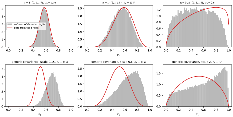
fig_17_S1, laplace_bridge. Not a reproduction of Figure 17.9, which needs a pretrained ImageNet network. Download: PDF · SVG17.3.10.3 Distillation
p. 664 The Monte Carlo predictive is \(S\) times slower than a deterministic network. Distillation fits a parametric student \(p_s(y\given\bm x)\) to the semi-parametric teacher \(p_t\) of (17.25) by minimising \(\E_{\bm x}[\KL(p_t(y\given\bm x)\,\|\,p_s(y\given\bm x))]\) (Hinton et al. 2014: "dark knowledge", the information in the teacher's probabilities beyond the one-hot labels; Korattikara et al. 2015 for an HMC teacher, "Bayesian dark knowledge"; Balan et al. 2016 and Gurau et al. 2018 for MC dropout). A student with a single Gaussian or softmax is less flexible than the teacher and tends to be over-confident; a mixture student is safer (Shen and Gao 2005; Tran et al. 2020).
Filling the gap 17.14: the distillation objective is a cross-entropy with soft labels p. 664
Why is distillation just "training on the teacher's probabilities"?
Derivation
\[ \KL(p_t\,\|\,p_s)=\sum_cp_{t,c}\log p_{t,c}-\sum_cp_{t,c}\log p_{s,c} \]. The first sum does not depend on the student, so minimising the KL over the student parameters is minimising the cross-entropy \(-\sum_cp_{t,c}\log p_{s,c}\) with the teacher's probabilities as soft labels; averaging over inputs and over the Monte Carlo teacher \(p_t=\frac1S\sum_sp(y\given\bm x,\th_s)\) gives the same as maximum likelihood on labels drawn from the teacher (infinitely many pseudo-labels per input). For a softmax student \(p_s=\softmax(\bm z)\), \(\partial\log p_{s,c'}/\partial z_c=\delta_{cc'}-p_{s,c}\), so \[ \frac{\partial}{\partial z_c}\Big(-\sum_{c'}p_{t,c'}\log p_{s,c'}\Big)=-p_{t,c}+p_{s,c}\sum_{c'}p_{t,c'}=p_{s,c}-p_{t,c}, \] the same simple gradient as for one-hot labels, with the teacher's probabilities in place of the labels. If the student's family is an exponential family, the minimiser matches the expected sufficient statistics of the teacher (moment matching); in particular a single Gaussian student matches the teacher's mean and variance, and a unimodal student cannot represent a bimodal teacher, which is why a mixture is preferred.
17.3.11 Tempered and cold posteriors
pp. 664–665, (17.32)–(17.35) For classification the likelihood is \(p(y\given\bm x,\th)=\Cat(y\given\softmax(f(\bm x;\th)))\) (17.32), but BNNs often predict better when the likelihood is raised to a power \(\alpha\) (Zhang et al. 2018; Wenzel et al. 2020): the tempered or power posterior \[ p_{\rm tempered}(\th\given\mathcal D)\propto p(\bm y\given\bm X,\th)^\alpha p(\th) \], i.e.
\[ \log p_{\rm tempered}(\th\given\mathcal D)=\alpha\log p(\bm y\given\bm X,\th)+\log p(\th)+\mathrm{const}. \tag{17.33}\]The cold posterior is \[ p_{\rm cold}(\th\given\mathcal D)\propto p(\th\given\bm X,\bm y)^{1/T} \], \[ \log p_{\rm cold}=\frac1T\log p(\bm y\given\bm X,\th)+\frac1T\log p(\th)+\mathrm{const} \] (17.34), "cold" when \(T<1\). For a Gaussian prior \(\N(\bm 0,\sigma_{\rm cold}^2\bm I)\) the factor \(1/T\) on the log prior is \(-\sum_i\theta_i^2/(2T\sigma^2_{\rm cold})\), the log of \(\N(\bm 0,T\sigma_{\rm cold}^2\bm I)\) (17.35), so the cold posterior is the tempered posterior with \(\alpha=1/T\) and prior variance \(\sigma^2_{\rm tempered}=T\sigma_{\rm cold}^2\). Kapoor et al. (2022) show that the cold-posterior effect comes from under-representing aleatoric (label) uncertainty: CIFAR labels are essentially certain, but a softmax classifier with a Bayesian posterior has high label uncertainty. With data augmentation, SGLD (Wenzel et al. 2020) effectively raises the likelihood to the power \(1/K\) for minibatches of size \(K\), which cold posteriors undo; Izmailov et al. (2021b) found the effect disappears without augmentation, and Kapoor et al. use a Dirichlet observation model to represent the absence of label noise and remove the effect even with augmentation. The curation hypothesis (Aitchison 2021) is a special case. Tempering is useful when the model is misspecified (Section 14.1.3, generalised variational inference; Knoblauch et al. 2022).
Filling the gap 17.15: what tempering does, in closed form, and the Gibbs variational principle pp. 664–665, (17.33)–(17.35)
The book gives the definitions and the equivalence (17.35). Here is the effect in a model where everything is exact, and the sense in which the tempered posterior is a "posterior" at all.
Derivation
Bayesian linear regression. With \(y=\bm\phi^\T\th+\varepsilon\), noise variance \(\sigma^2\), prior \(\N(\bm 0,\tau^2\bm I)\), the posterior precision is \(\bm A=\bm\Phi^\T\bm\Phi/\sigma^2+\bm I/\tau^2\) and the mean \(\bm A^{-1}\bm\Phi^\T\bm y/\sigma^2\). (a) Tempering: \[ p^\alpha(\bm y\given\th)\propto\exp(-\alpha\|\bm y-\bm\Phi\th\|^2/(2\sigma^2)) \] is the likelihood with noise variance \(\sigma^2/\alpha\). The tempered posterior is Gaussian with precision \(\alpha\bm\Phi^\T\bm\Phi/\sigma^2+\bm I/\tau^2\) and mean \((\alpha\bm\Phi^\T\bm\Phi/\sigma^2+\bm I/\tau^2)^{-1}\alpha\bm\Phi^\T\bm y/\sigma^2\): the mean moves towards the data-only fit (the prior counts for less) and the covariance shrinks (\(\alpha>1\)). (b) Cooling: \(p^{1/T}\) multiplies the whole log posterior by \(1/T\), the precision becomes \(\bm A/T\) and the mean is unchanged: the cold posterior is the exact posterior with its covariance multiplied by \(T\), the same mean. (c) Equivalence (17.35): the cold posterior with prior \(\sigma_{\rm cold}^2\) equals the tempered posterior with \(\alpha=1/T\) and prior \(T\sigma^2_{\rm cold}\) (precision \[ \alpha\bm\Phi^\T\bm\Phi/\sigma^2+\bm I/(T\sigma_{\rm cold}^2)=\bm A/T \] when \(\tau=\sigma_{\rm cold}\)): both multiply every log term by \(1/T\). (d) Data augmentation. If augmentation makes the effective power of the likelihood \(1/K\) (as Kapoor et al. show for the SGLD of Wenzel et al.), a cold posterior with \(\alpha=K\), i.e. \(T=1/K\), restores the power 1. All of (a)–(c) were confirmed numerically.
Why the power posterior is a legitimate object. For a loss \(\ell(\th)=-\log p(\mathcal D\given\th)\) and \(\alpha>0\), the distribution \(q\) minimising \(\E_q[\alpha\ell(\th)]+\KL(q\,\|\,p)\) is the tempered posterior: for any \(q\), \[ \E_q[\alpha\ell]+\KL(q\|p)=\KL(q\,\|\,q^\star)-\log Z_\alpha \] with \(q^\star=p\,e^{-\alpha\ell}/Z_\alpha\) and \(Z_\alpha=\int p\,e^{-\alpha\ell}\d\th\), which is minimised at \(q=q^\star\) (Gibbs variational principle; Bissiri et al. 2016, "general Bayesian updating"). Dividing by \(\alpha\) shows it is the same as minimising the expected loss with the KL term down-weighted by \(\beta=1/\alpha\): this is the \(\beta\) in the generalised variational continual learning objective (17.55) of Section 17.5.4.
17.4 Generalization in Bayesian deep learning
p. 665 Why does "being Bayesian" improve accuracy and generalisation, and when does it not?
17.4.1 Sharp vs flat minima
pp. 665–666, Figure 17.10 Some optimisers find "needles in haystacks": narrow, deep holes in the loss, with very low training loss (sharp minima, Figure 17.10 right). Such solutions tend to overfit; flat minima are more robust and generalise better (Hochreiter and Schmidhuber 1997). A flat minimum is a region with much posterior uncertainty, whose samples cannot memorise irrelevant details of the training set (Achille and Soatto 2018), and it has a short description length: fewer bits are needed to specify the weights to the precision that keeps the loss low (MacKay 2003). SGD finds flat minima because its noise keeps it out of narrow regions (Section 12.5.7), and flat regions occupy much more volume in high dimension. Smith and Le (2018) show that the probability that SGD enters a basin \(A\) is proportional to \(\int_Ae^{-L(\th)}\d\th\), the evidence of that region (Section 3.8.1), which is invariant to reparameterisation, unlike measures of sharpness (against Dinh et al. 2017). If a single solution must be used, a flat one best approximates the Bayesian average (17.1); a fuller average selects for flatness automatically, without having to define it.
Filling the gap 17.16: the Occam factor of a basin, and why it, unlike sharpness, is parameterisation invariant pp. 665–666
The book says the SGD basin probability is "proportional to the model evidence for that region" and that the evidence is parameterisation invariant. Both claims need one computation each.
Derivation
The Laplace evidence of a basin. Let \(E(\th)=-\log p(\mathcal D\given\th)-\log p(\th)\) have a minimum at \(\th^\star\) with Hessian \(\bm H\succ0\). Then \[ \int_Ae^{-E(\th)}\d\th\approx e^{-E(\th^\star)}\int e^{-\frac12(\th-\th^\star)^\T\bm H(\th-\th^\star)}\d\th=p(\mathcal D\given\th^\star)\,p(\th^\star)\,(2\pi)^{P/2}|\bm H|^{-1/2}. \] The factor \(p(\th^\star)(2\pi)^{P/2}|\bm H|^{-1/2}\) is the Occam factor: the fraction of the prior volume occupied by the posterior mode. For equal best-fit loss, a basin with large \(|\bm H|\) (sharp) has a small factor and small evidence, and by the Smith–Le result is entered by SGD with small probability. In terms of the eigenvalues \(\lambda_i\) of \(\bm H\), the log Occam factor contains \(-\frac12\sum_i\log\lambda_i\): every flat direction (\(\lambda_i\) small) adds to the evidence.
Invariance. The exact evidence does not depend on how the weights are parameterised. Let \(\th=g(\bm\varphi)\) with \(g\) a smooth bijection and Jacobian \(\bm J=\partial\th/\partial\bm\varphi\). The prior density transforms as \(p_\varphi(\bm\varphi)=p_\theta(g(\bm\varphi))|\det\bm J|\), and \[ \int p(\mathcal D\given g(\bm\varphi))p_\varphi(\bm\varphi)\d\bm\varphi=\int p(\mathcal D\given\th)p_\theta(\th)\d\th \] by change of variables. Its Laplace approximation shares this property exactly for an affine map \(\th=\bm A\bm\varphi\) (constant \(\bm J=\bm A\)): modes correspond, \(\bm H_\varphi=\bm A^\T\bm H_\theta\bm A\), so \[ -\frac12\log|\bm H_\varphi|=-\frac12\log|\bm H_\theta|-\log|\det\bm A| \], while \[ \log p_\varphi(\bm\varphi^\star)=\log p_\theta(\th^\star)+\log|\det\bm A| \]; the two Jacobian terms cancel in the Occam factor \(\log p(\th^\star)-\frac12\log|\bm H|\). (For a non-linear map the Laplace approximation is taken around a different point and is invariant only up to its accuracy.) By contrast, the largest eigenvalue or the trace of the Hessian are not invariant at all: for the ReLU network \(f=w_2\max(w_1x,0)\), the reparameterisation \(w_1\to cw_1\), \(w_2\to w_2/c\) leaves \(f\), the loss and the evidence unchanged, but at a zero-residual solution the only non-zero Hessian eigenvalue \(x^2(w_1^2+w_2^2)\) (for a single input \(x>0\)) becomes \(x^2(c^2w_1^2+w_2^2/c^2)\), arbitrarily large, so "sharpness" can be made as large as we like (Dinh et al. 2017). The book's argument that preferring flat minima is parameterisation-free when stated through the evidence is therefore correct; it applies to the volume \(\int_Ae^{-L}\), not to the sharpness. A numerical experiment confirmed the cancellation in an exactly solvable Gaussian model.
17.4.2 Mode connectivity and the loss landscape
pp. 666–667, Figure 17.11 Networks have many low-loss solutions that explain the data differently. Garipov et al. (2018) showed that two independently trained SGD solutions can be joined by a curve along which the training loss stays near zero (mode connectivity), yet the points on the curve give very different functions (Figure 17.11: predictions on a one-dimensional problem along a curve between two MAP estimates). A Bayesian model average over such functions beats a single flat solution (Izmailov et al. 2019), and there are large simplexes of low-loss solutions (Benton et al. 2021). Figure 17.11 reproduces the experiment: two tanh MLPs (1–40–40–1) trained from different initialisations on 28 points with a gap, a quadratic Bezier curve \(\th(t)=(1-t)^2\th_1+2t(1-t)\bm\phi+t^2\th_2\) whose single control point \(\bm\phi\) is trained to minimise the expected loss over \(t\sim\mathrm{Uniform}(0,1)\), and the loss on the plane through the two modes and the curve's mid-point.
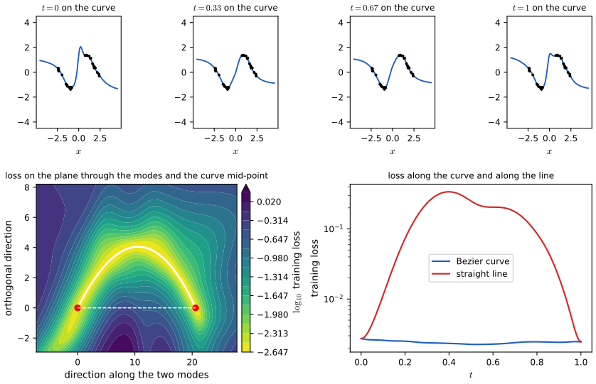
fig_17_11, mode_connectivity. Reproduces Murphy (2023), Figure 17.11 (our own data and networks). Download: PDF · SVG17.4.3 Effective dimensionality of a model
pp. 667–668, (17.36), Figure 17.12 Modern DNNs have millions of parameters, but most are not well determined by the data. Following Maddox et al. (2020) and MacKay (1992), the effective dimensionality is
\[ N_{\rm eff}(\bm H,c)=\sum_{i=1}^k\frac{\lambda_i}{\lambda_i+c}, \tag{17.36}\]with \(\lambda_i\) the eigenvalues of the Hessian at a mode and \(c>0\) a regularisation constant: it counts the parameters that are well determined. A flat minimum has many small eigenvalues and low effective dimension, so inference can be done in a low-dimensional subspace (Izmailov et al. 2019) and the network is compressible; of two models with the same training loss, the one with lower \(N_{\rm eff}\) compresses the data better. Figure 17.12 shows for CNNs on CIFAR-100 that \(N_{\rm eff}\) tracks generalisation among models with near-zero training loss, that the parameter count alone does not, that wide shallow models overfit, and that depth lowers the effective dimension. (That figure needs GPU-scale training and is not reproduced; Figure 17.S6 shows the same quantities on a small problem.)
Filling the gap 17.17: three meanings of \(N_{\rm eff}\) p. 667, (17.36)
The book says that \(N_{\rm eff}\) "counts the number of well-determined parameters". Here is a precise statement for the linear-Gaussian case, which is the local model of a network at a mode.
Derivation
Take \(\bm y=\bm\Phi\th+\bm\varepsilon\), noise variance \(\sigma^2\), prior \(\th\sim\N(\bm 0,c^{-1}\bm I)\). The Hessian of the negative log likelihood is \(\bm H=\bm\Phi^\T\bm\Phi/\sigma^2\), with eigenvalues \(\lambda_i\ge0\) and eigenvectors \(\bm v_i\). (a) Ridge degrees of freedom. The posterior mean fit is \[ \hat{\bm y}=\bm\Phi(\bm\Phi^\T\bm\Phi+\sigma^2c\bm I)^{-1}\bm\Phi^\T\bm y=\bm S\bm y \], with trace \[ \Tr\bm S=\sum_i\frac{\sigma^2\lambda_i}{\sigma^2\lambda_i+\sigma^2c}=\sum_i\frac{\lambda_i}{\lambda_i+c}=N_{\rm eff} \] (using the singular values of \(\bm\Phi\): \[ \Tr[\bm\Phi(\bm\Phi^\T\bm\Phi+\mu\bm I)^{-1}\bm\Phi^\T]=\sum_i s_i^2/(s_i^2+\mu) \] with \(s_i^2=\sigma^2\lambda_i\), \(\mu=\sigma^2c\)). This is the effective degrees of freedom of the ridge smoother (the trace of the hat matrix). (b) Fraction of prior variance removed. In direction \(\bm v_i\) the prior variance is \(1/c\) and the posterior variance is \(1/(\lambda_i+c)\), so the fraction removed is \(1-c/(\lambda_i+c)=\lambda_i/(\lambda_i+c)\), and \(N_{\rm eff}=P-c\,\Tr\bm\Sigma_{\rm post}\), the same \(\gamma\) as in Filling the gap 17.3. (c) Information. The mutual information between \(\th\) and \(\bm y\) is \(I=\tfrac12\sum_i\log(1+\lambda_i/c)\). Since \(\log(1+x)\ge x/(1+x)\) for \(x\ge0\), \(N_{\rm eff}\le2I\), with near equality when all \(\lambda_i\ll c\) (the weak-data regime). As \(c\to0\), \(N_{\rm eff}\to\operatorname{rank}\bm H\); as \(c\to\infty\), \(N_{\rm eff}\to0\); it decreases monotonically in \(c\). For a network, \(\bm H\) is the Hessian (or the GGN) of the negative log likelihood at the mode and \(c\) the prior precision; the interpretation as a local linear-Gaussian model is exact for the linearised network of Filling the gap 17.5. The three expressions were confirmed numerically on random designs.
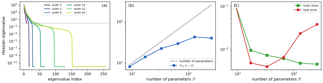
fig_17_S6, width_study. A small-scale analogue of Figure 17.12 (not a reproduction). Download: PDF · SVG17.4.4 The hypothesis space of DNNs
pp. 668–669, Figure 17.13 Zhang et al. (2017) found that CNNs fit CIFAR-10 with random labels perfectly and yet generalise on the true labels, which seems to contradict classical learning theory. The Bayesian resolution (Wilson and Izmailov 2020): a CNN is flexible enough (a universal approximator) to represent random labels, but its architecture is a prior over patterns, and a data set with random labels gets very low marginal likelihood because it violates the prior, while a data set whose labels follow patterns in the inputs gets much higher marginal likelihood. Gaussian processes behave in the same way. One should distinguish the support of a model (the functions it can represent) from the inductive bias (the distribution over that support). We want large support and a bias that puts mass on the functions we expect; then the posterior collapses on the truth after a few observations (Figure 17.13 sketches a linear model, an MLP and a CNN).
Filling the gap 17.18: the evidence is a distribution over data sets, so flexibility is paid for pp. 668–669
"Such solutions receive very low marginal likelihood" follows from a conservation law.
Derivation
Conservation of evidence. For a fixed model \(\mathcal M\) and fixed inputs, the marginal likelihood \[ p(\bm y\given\mathcal M)=\int p(\bm y\given\th)p(\th\given\mathcal M)\d\th \] is a probability distribution over labellings \(\bm y\): it is non-negative and, by Fubini, \[ \sum_{\bm y}p(\bm y\given\mathcal M)=\int p(\th\given\mathcal M)\sum_{\bm y}p(\bm y\given\th)\d\th=1 \]. Hence the number of labellings with evidence at least \(\delta\) is at most \(1/\delta\) (Markov's inequality in counting form: \(\delta\,|\{\bm y:p\ge\delta\}|\le\sum p=1\)). With \(N\) binary labels there are \(2^N\) labellings, and for \(\delta=2^{k-N}\) at most \(2^{N-k}\) of them, a fraction \(2^{-k}\), can have evidence \(\ge\delta\). If a model can fit every labelling equally well, its prior must spread mass over all of them and each gets about \(2^{-N}\).
Structured against random labels. A model whose prior concentrates on smooth functions puts most of its mass on the few labellings that vary smoothly with the input; it can still represent random labellings (support), but only with a small prior probability, \(\ll2^{-N}\) for most of them. Figure 17.S7 shows this for a Gaussian process with an RBF kernel (an infinitely wide network's limit): on 50 points of a smooth function, a model with length scale 1.5 assigns the true labels a log evidence of \(+24.7\) and 300 shuffled copies a log evidence of about \(-1013\) on average; a very flexible model (length scale 0.03, which behaves like white noise and can fit nearly anything) gives \(-47\) to the true labels and \(-99\) on average to the shuffled ones, both far below the \(+24.7\) of the matched model (it pays the Occam penalty on every data set), and the model with length scale 0.4 is in between. The data with structure are explained by the model with the matching inductive bias, and a random-label data set is "a priori unlikely" without being outside the support.
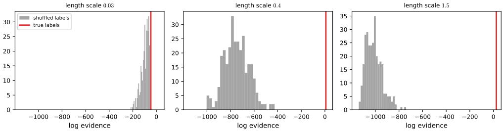
fig_17_S7, gp_log_evidence. Download: PDF · SVG17.4.5 PAC-Bayes
p. 669, (17.37) PAC-Bayes bounds (McAllester 1999; Langford and Caruana 2002; Guedj 2019; Alquier 2021) yield non-vacuous generalisation bounds for large stochastic networks whose weights are drawn from a distribution \(Q\) (Neyshabur et al. 2017; Dziugaite and Roy 2017). The gap between the generalisation error and the training error is bounded by a term of the form
\[ \sqrt{\frac{\KL(Q\,\|\,P)+c}{2(N-1)}}, \tag{17.37}\]with \(c\) a constant (it depends on the confidence level and on \(N\) only logarithmically), \(P\) a prior and \(Q\) any distribution, which can be optimised. The authors stress that this view is complementary to the Bayesian marginalisation of this chapter: the bound is about the risk of a single sample from \(Q\), not of the average, is not prescriptive (reducing the number of parameters or using compact priors does not typically improve generalisation) and is only logarithmically affected by multimodal averaging, so it is loose.
Filling the gap 17.19: a proof of a PAC-Bayes bound of the form (17.37) p. 669, (17.37)
The book quotes (17.37) with an unspecified constant. The change-of-measure proof is short, and shows where each term comes from.
Derivation
Setting. A loss \(\ell(\th;z)\in[0,1]\), the risk \(L(\th)=\E_z\ell(\th;z)\) and the empirical risk \(\hat L(\th)=\frac1N\sum_n\ell(\th;z_n)\) on \(N\) i.i.d. examples. \(P\) is a prior chosen before seeing the data and \(Q\) any distribution (it may depend on the data). \(L(Q)=\E_{\th\sim Q}L(\th)\), \(\hat L(Q)=\E_{\th\sim Q}\hat L(\th)\).
Step 1 (change of measure; Donsker–Varadhan). For any measurable \(g\), \(\E_Q[g]\le\KL(Q\,\|\,P)+\log\E_P[e^g]\). Proof: with \(R=\E_P[e^g]\) and \(\tilde P=Pe^g/R\), \(0\le\KL(Q\,\|\,\tilde P)=\KL(Q\,\|\,P)-\E_Q[g]+\log R\).
Step 2 (Hoeffding). For fixed \(\th\), \(L(\th)-\hat L(\th)\) is the mean of \(N\) independent centred variables with range 1, so \[ \E_S\exp(\lambda(L(\th)-\hat L(\th)))\le\exp(\lambda^2/(8N)) \] (Hoeffding's lemma, applied to each of the \(N\) terms with \(\lambda/N\)).
Step 3 (Markov, with Fubini). \[ \E_S\E_P\exp(\lambda(L-\hat L))=\E_P\E_S\exp(\lambda(L-\hat L))\le e^{\lambda^2/(8N)} \], so by Markov's inequality with probability at least \(1-\delta\) over \(S\), \(\E_P\exp(\lambda(L-\hat L))\le e^{\lambda^2/(8N)}/\delta\). Because \(P\) does not depend on \(S\), the exchange is legitimate.
Step 4. On that event, for every \(Q\), Step 1 with \(g=\lambda(L-\hat L)\) gives \[ \lambda(L(Q)-\hat L(Q))\le\KL(Q\,\|\,P)+\lambda^2/(8N)+\log(1/\delta) \], i.e. \[ L(Q)\le\hat L(Q)+\frac{\KL(Q\,\|\,P)+\log(1/\delta)}{\lambda}+\frac\lambda{8N}. \] For \(\lambda=\sqrt{8N(\KL+\log(1/\delta))}\) the right side is \(\hat L(Q)+\sqrt{(\KL(Q\|P)+\log(1/\delta))/(2N)}\), the form (17.37). \(\lambda\) must be fixed before the data, so this choice presupposes a guess of the KL. A union bound over a grid of \(\lambda\), or the moment bound of Maurer (2004), gives a bound of the same order that holds for every \(Q\) simultaneously, with \(c=\log(2\sqrt N/\delta)\) and denominator \(2N\) (the printed \(2(N-1)\) is a convention of the original statements). The book's wording is therefore right in form: the gap is of order \(\sqrt{\KL/N}\), small only when \(Q\) is close to \(P\) and \(N\) is large.
Why it is loose for ensembles. The KL enters only through its square root divided by \(\sqrt N\); averaging over \(M\) modes changes \(\KL(Q\|P)\) by at most \(\log M\), a logarithmic effect, however large the change in the predictive accuracy. A simulation with a one-dimensional threshold classifier and Gaussian \(P,Q\) confirmed that the bound holds with the stated frequency and is far from tight.
17.4.6 Out-of-distribution generalization for BNNs
pp. 669–671, Figure 17.14 Bayesian methods are often assumed to be more robust under distribution shift (Chapter 19) because they represent more uncertainty; there are subtleties.
17.4.6.1 BMA can give poor results with default priors
pp. 670–671, Figure 17.14 Deep ensembles are less over-confident than point estimates under some covariate shifts (Ovadia et al. 2019), but Izmailov et al. (2021b) noted that HMC, arguably the most accurate posterior approximation, often does worse under shift. This is a foundational issue of Bayesian model averaging with default priors, not of HMC (Izmailov et al. 2021a). MNIST digits have black corner pixels: first-layer weights attached to them multiply zero, so they can take any value without affecting the outputs. MAP training or a deep ensemble with a Gaussian prior drives them to zero, so corruption of those pixels is ignored; but their posterior is the prior, so a BMA multiplies the corruption by random numbers drawn from the prior. Figure 17.14(b, c) shows the first-layer weights of an HMC sample (noisy) and of the MAP (near zero at the boundary); panel (a) shows a Bayesian ResNet-20 under pixelation 25 percentage points worse than MAP. The general statement (Izmailov et al. 2021a) covers any linear dependence among the training inputs (data on a hyperplane): a shift orthogonal to it leaves the posterior equal to the prior in that direction. The fix is a prior aligned with the principal components of the inputs, the EmpCov prior \(p(\bm w_1)=\N(\bm 0,\alpha\hat{\bm\Sigma}+\epsilon\bm I)\) with \(\hat{\bm\Sigma}=\frac1{n-1}\sum_i\bm x_i\bm x_i^\T\), \(\alpha>0\) and a small \(\epsilon>0\) (to keep it positive definite).
Filling the gap 17.20: with a rank-deficient design the posterior equals the prior along the null space pp. 670–671
The book gives the statement and the remedy; here is the proof, in the model where it is exact, and the effect of the EmpCov prior.
Derivation
Posterior on the null space. Let \(\bm X\in\R^{N\times D}\) have rank \(r<D\), null space \(\mathcal N=\{\bm v:\bm X\bm v=\bm0\}\) (dimension \(D-r\)), and consider \(\bm y=\bm X\bm w+\bm\varepsilon\), prior \(\bm w\sim\N(\bm 0,\tau^2\bm I)\). The posterior precision is \(\bm X^\T\bm X/\sigma^2+\bm I/\tau^2\), and for \(\bm v\in\mathcal N\) it acts as \(\bm v/\tau^2\): the null space is an eigenspace with eigenvalue \(1/\tau^2\). Hence \(\cov(\bm w\given\mathcal D)\bm v=\tau^2\bm v\) and the projection of \(\bm w\) on \(\mathcal N\) has the same distribution as under the prior, and is independent of the projection on the row space. The posterior mean \(\bm m=\bm A^{-1}\bm X^\T\bm y/\sigma^2\) lies in the row space (\(\bm A\) preserves it and \(\bm X^\T\bm y\) is in it): the MAP, and the posterior mean of a linear model, put zero weight on the null directions.
Shifted test inputs. Let \(\bm x_*=\bm x+\bm\delta\) with \(\bm\delta\in\mathcal N\) (a shift the training data never explored). The posterior mean prediction is \(\bm m^\T\bm x_*=\bm m^\T\bm x\), unchanged, but the predictive variance acquires \(\tau^2\|\bm\delta\|^2\) from the null space. For a network, each posterior sample has a random first-layer weight vector in those directions, \(\bm w_1\sim\N(\bm 0,\tau^2)\) along \(\mathcal N\), and the corruption \(\bm\delta\) enters the hidden units through it: \[ \bm w_1^\T(\bm x+\bm\delta)=\bm w_1^\T\bm x+\bm w_1^\T\bm\delta \], a random term of standard deviation \(\tau\|\bm\delta\|\) that the nonlinearity does not average away. Averaging many samples, the BMA is a mixture of functions that are randomly perturbed by the shift, and its accuracy falls. The MAP and deep ensembles of MAPs have \(\bm w_1\bm\delta=0\).
The EmpCov prior. With prior covariance \(\alpha\hat{\bm\Sigma}+\epsilon\bm I\) the prior variance along a null direction \(\bm v\) (\(\bm X\bm v=\bm0\), so \(\hat{\bm\Sigma}\bm v=\bm0\)) is \(\epsilon\) and along a data direction it is \(\alpha\lambda_i(\hat{\bm\Sigma})+\epsilon\). The shift contributes variance \(\epsilon\|\bm\delta\|^2\) instead of \(\tau^2\|\bm\delta\|^2\), and \(\epsilon\) can be made very small. Prior variances along the directions the data do explore stay large, so no flexibility is lost where it is needed. This is demonstrated by the numbers in Figure 17.S5 and the demonstration, and confirmed on the linear model above.
p. 670 Figure 17.S5 and the covariate-shift demonstration reproduce the phenomenon in miniature. A one-hidden-layer tanh network with four units has a "dead" second input, exactly zero in the training set; its four weights have no influence on the likelihood, so their posterior is their prior (as above), while the other 13 parameters have an HMC posterior. The test inputs are a one-dimensional band problem with the dead input corrupted by \(s\) times a standard normal.
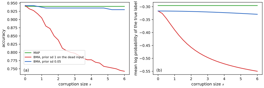
fig_17_S5, shift_posterior. Download: PDF · SVG17.4.6.2 BNNs can be overconfident on OOD inputs
pp. 671–672, Figure 17.15 We would like a model to say "I don't know" (probability 0.5) far from the training data. "Exact" inference (an MLP fitted with SGLD on MNIST is less over-confident than SGD on Fashion-MNIST inputs, Section 19.3.3.1) does not always achieve this. Figure 17.15 trains an MLP (8–16–16–8 ReLU units, sigmoid output) on a two-moons problem and shows predictions near a blob of OOD inputs (green) far from the training data, for eight methods: SGD, a deep ensemble, MC dropout, bootstrap, MCMC, variational inference, a Gaussian process classifier and SNGP. Only the GP and SNGP, which have an explicit distance-aware layer, go to 0.5 away from the data in the book. The lesson: being Bayesian only helps when the hypothesis class is good; a standard MLP with standard Gaussian priors has almost no prior mass on a compact decision region like that of the GP (Section 17.4.4), so one should use as rich a model class as can be afforded.
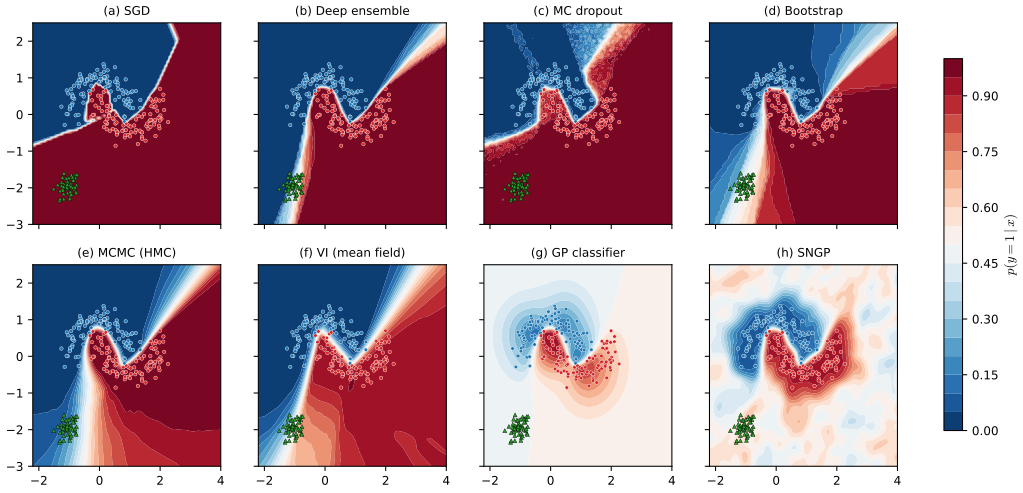
fig_17_15, moons_predictors. Reproduces Murphy (2023), Figure 17.15 (with 200 instead of 1000 training points and our own samplers; the book plots a standard deviation, we plot the probability itself). Download: PDF · SVGFilling the gap 17.21: ReLU networks are over-confident far from the data, for every parameter vector pp. 671–672
Why do the standard networks of Figure 17.15 not return 0.5 far away? A short argument shows they cannot, for any weights.
Derivation
Piecewise-linear networks are linear on rays. A ReLU network \(f:\R^d\to\R^C\) is continuous and piecewise affine with finitely many linear regions. Fix a direction \(\bm u\ne\bm0\). The ray \(\{t\bm u:t\ge0\}\) crosses each region in an interval, and there are finitely many regions, so for \(t\ge t_0\) it stays in one region, where \(f(\bm x)=\bm U\bm x+\bm c\). Hence \(\bm z(t)=f(t\bm u)=t\,\bm a+\bm c'\) with \(\bm a=\bm U\bm u\), a linear function of \(t\) with slope \(\bm a\) (Hein et al. 2019).
Softmax saturates. If \(\bm a\) has a unique largest component \(a_k\) with margin \(\gamma=a_k-\max_{j\ne k}a_j>0\) (true for generic weights), then \(\softmax(\bm z(t))_k\ge1-(C-1)e^{-\gamma t+O(1)}\to1\). For a binary sigmoid output the logit \(t\,a+c'\) tends to \(\pm\infty\) and the probability to 0 or 1, exponentially fast. So for each fixed \(\th\) the prediction far away is a one-hot vector in a direction-dependent class: arbitrarily confident, whatever the weights.
What a posterior average does. The BMA probability of class \(k\) in the limit is \(\Pr_{\th\sim p(\th\given\mathcal D)}[\arg\max_ja_j(\th)=k]\), the posterior probability that class \(k\) wins in the asymptotic direction. It equals 0.5 only if the posterior is split evenly over classes in that direction, which nothing in a standard Gaussian prior or in the training data forces; a posterior concentrated around one mode (Laplace, VI, a single basin of HMC, a deep ensemble whose members agree) predicts one class with probability near 1. Far from the data the logits of different posterior samples disagree by amounts \(\propto t\), but the probabilities only disagree if the winning class differs. A GP with an RBF kernel instead reverts to its prior mean (zero logit, probability 0.5) away from the data, because the kernel decays; SNGP imitates that. A numerical experiment with random ReLU networks confirmed linear growth of the logit along rays and saturation of the sigmoid.
17.4.7 Model selection for BNNs
p. 671 The marginal likelihood has historically selected architectures and hyperparameters (MacKay 1992), and Laplace-based estimates scale it to large networks (Immer et al. 2021; Daxberger et al. 2021). Lotfi et al. (2022) argue that the conditional marginal likelihood is much better (Section 3.8.5; notes, Section 3.8), because the marginal likelihood measures prior predictive performance, which includes the cost of the first few observations, while generalisation concerns the performance after learning.
17.5 Online inference
p. 672 So far inference was in batch. In sequential Bayesian inference the data arrive as a stream, \[ p(\th\given\mathcal D_{1:t})\propto p(\mathcal D_t\given\th)\,p(\th\given\mathcal D_{1:t-1}) \], and the posterior after step \(t-1\) is the prior for step \(t\). The methods below are used for continual learning (Section 19.7).
17.5.1 Sequential Laplace for DNNs
pp. 672–673, (17.38)–(17.40) Ritter et al. (2018) extended the Laplace approximation to the sequential setting. Let \[ p(\th\given\mathcal D_{1:t-1})\approx\N(\th\given\bm\mu_{t-1},\bm\Lambda_{t-1}^{-1}) \] (Kronecker-factored precision). The new mean solves the MAP problem
\[ \bm\mu_t=\argmax_\th\ \log p(\mathcal D_t\given\th)+\log p(\th\given\mathcal D_{1:t-1})=\argmax_\th\ \log p(\mathcal D_t\given\th)-\tfrac12(\th-\bm\mu_{t-1})^\T\bm\Lambda_{t-1}(\th-\bm\mu_{t-1}) \tag{17.38, 17.39}\](see the correction below: the quadratic form uses the precision \(\bm\Lambda_{t-1}\), not its inverse as printed), and the new precision adds the Hessian at \(\bm\mu_t\),
\[ \bm\Lambda_t=\lambda\bm H(\bm\mu_t)+\bm\Lambda_{t-1}, \tag{17.40}\]where \(\lambda\ge0\) trades the new data against the old. With a diagonal precision this is a quadratic penalty that keeps the new solution near the old one: elastic weight consolidation (EWC; Kirkpatrick et al. 2017).
Filling the gap 17.22: sequential Laplace and EWC are exact for a linear-Gaussian model; the precision in (17.39) pp. 672–673
The book gives the recursion without checking it. It has one misprint and one exact special case.
Derivation
The misprint. With \[ p(\th\given\mathcal D_{1:t-1})\approx\N(\bm\mu_{t-1},\bm\Lambda_{t-1}^{-1}) \], the log density is \(-\frac12(\th-\bm\mu_{t-1})^\T\bm\Lambda_{t-1}(\th-\bm\mu_{t-1})+\mathrm{const}\), with the precision \(\bm\Lambda_{t-1}\) in the middle. (17.39) prints \(\bm\Lambda_{t-1}^{-1}\) (the covariance), which would penalise deviations in the directions that are well determined least. (The transpose is also missing in the book's expression.)
Exactness. Let \(\bm y_t=\bm\Phi_t\th+\bm\varepsilon_t\), noise variance \(\sigma^2\), prior \(\N(\bm\mu_0,\bm\Lambda_0^{-1})\), and use \(\lambda=1\) with the exact Hessian of the negative log likelihood, \(\bm H_t=\bm\Phi_t^\T\bm\Phi_t/\sigma^2\) (independent of \(\th\)). Claim: \(\bm\mu_t,\bm\Lambda_t\) from (17.38)–(17.40) are the mean and precision of the exact posterior given \(\mathcal D_{1:t}\). By induction: if \[ p(\th\given\mathcal D_{1:t-1})=\N(\bm\mu_{t-1},\bm\Lambda_{t-1}^{-1}) \], then \[ p(\th\given\mathcal D_{1:t})\propto\exp\big(-\tfrac{1}{2\sigma^2}\|\bm y_t-\bm\Phi_t\th\|^2-\tfrac12(\th-\bm\mu_{t-1})^\T\bm\Lambda_{t-1}(\th-\bm\mu_{t-1})\big) \], a Gaussian whose mode is the solution of (17.39) and whose precision is the Hessian of the exponent, \(\bm H_t+\bm\Lambda_{t-1}=\bm\Lambda_t\). So in the linear-Gaussian case sequential Laplace equals batch Bayes (and the order of the batches does not matter). For a network the Hessian is evaluated at \(\bm\mu_t\) and the model is only locally linear, so the recursion is an approximation whose quality degrades as the posterior moves; a diagonal \(\bm\Lambda\) (EWC) discards correlations and is exact only when the data matrix has orthogonal columns. Both statements were verified numerically (batch and sequential agree to rounding error, and a diagonal precision does not).
17.5.2 Extended Kalman filtering for DNNs
p. 673, (17.41)–(17.44), Figure 17.16 For a linear regression model with known noise variance, \[ p(y_t\given\bm u_t,\th,\sigma^2)=\N(y_t\given\th^\T\bm u_t,\sigma^2) \] (17.41), the Kalman filter with the weights as the (static) state computes the exact posterior \(p(\th\given\mathcal D_{1:t},\sigma^2)\): recursive least squares (Section 29.7.2). For nonlinear regression, \[ p(y_t\given\bm u_t,\th,\sigma^2)=\N(y_t\given f(\th,\bm u_t),\sigma^2) \] (17.42), the extended Kalman filter (Section 8.3.2, notes; Singhal and Wu 1989) linearises \(f\) around the current mean: the dynamics are the identity, \(\th_t=\th_{t-1}+\bm q\), so the parameters are propagated unchanged except for artificial process noise \(\bm Q_t=q\bm I\) with a small \(q\) that lets the parameters drift slowly (it can be annealed from large to near zero), and the observation noise is \(R_t=\sigma^2\).
17.5.2.1 Example
pp. 673–674, (17.43)–(17.44) The data are drawn from the true function \(h^\star(u)=u-10\cos(u)\sin(u)+u^3\) (17.43) (the book prints \(x\) for the first term, which should be \(u\)) with Gaussian noise \(\sigma=3\), and fitted with an MLP with \(H\) hidden units, \(f(\th,u)=\bm W_2\tanh(\bm W_1u+\bm b_1)+b_2\) (17.44) with \(\bm W_1\in\R^{H\times1}\), \(\bm b_1\in\R^H\), \(\bm W_2\in\R^{1\times H}\), \(b_2\in\R\). With \(H=6\) there are \(D=19\) parameters. The prior is \(\N(\th_0,\bm\Sigma_0)\) with \(\bm\Sigma_0=100\bm I\) (the mean cannot be 0, where the gradient vanishes, so a random vector is used). Figure 17.16 shows the fit after 10, 20, 30 and 200 observations: the model adapts without a learning rate, and the predictions become more confident as the posterior concentrates.
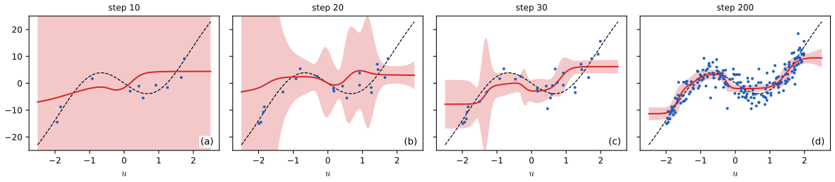
fig_17_16, ekf_mlp. Reproduces Murphy (2023), Figure 17.16. Download: PDF · SVGFilling the gap 17.23: the EKF update as a Gauss–Newton step, recursive least squares, and the role of \(q\) pp. 673–674; supplement 17.1.1
The book defers the algebra of the update to the supplement. Here it is derived, and its three properties that matter for networks are proved.
Derivation
The update. State \(\th_k=\th_{k-1}+\bm w_k\), \(\bm w_k\sim\N(\bm0,\bm Q)\); observation \(\bm y_k=h(\th_k)+\bm r_k\), \(\bm r_k\sim\N(\bm0,\bm R)\). Let the prior at step \(k\) be \(\N(\bm\mu,\bm\Sigma)\) (after adding \(\bm Q\)) and linearise \(h(\th)\approx h(\bm\mu)+\bm H(\th-\bm\mu)\), \(\bm H=\partial h/\partial\th|_{\bm\mu}\) (\(N\times M\)). Then \((\th,\bm y)\) is jointly Gaussian with \(\cov(\th,\bm y)=\bm\Sigma\bm H^\T\), \(\var\bm y=\bm S=\bm R+\bm H\bm\Sigma\bm H^\T\), and Gaussian conditioning gives \[ \bm K=\bm\Sigma\bm H^\T\bm S^{-1},\qquad\bm\mu^+=\bm\mu+\bm K(\bm y-h(\bm\mu)),\qquad\bm\Sigma^+=\bm\Sigma-\bm K\bm H\bm\Sigma. \]
Information form, and a Gauss–Newton step. By the Woodbury identity \(\bm\Sigma^{+\,-1}=\bm\Sigma^{-1}+\bm H^\T\bm R^{-1}\bm H\) and \(\bm K=\bm\Sigma^+\bm H^\T\bm R^{-1}\), so \[ \bm\mu^+=\bm\mu+\bm\Sigma^+\bm H^\T\bm R^{-1}(\bm y-h(\bm\mu)) \]. This is exactly one Gauss–Newton step started from \(\bm\mu\) on \[ J(\th)=\tfrac12\|\bm y-h(\th)\|^2_{\bm R^{-1}}+\tfrac12(\th-\bm\mu)^\T\bm\Sigma^{-1}(\th-\bm\mu) \]: the Gauss–Newton step is \(\bm\mu-(\bm H^\T\bm R^{-1}\bm H+\bm\Sigma^{-1})^{-1}\nabla J(\bm\mu)\) with \(\nabla J(\bm\mu)=-\bm H^\T\bm R^{-1}(\bm y-h(\bm\mu))\). So the EKF is online, second-order optimisation with a matrix-valued learning rate \(\bm\Sigma^+\bm H^\T\bm R^{-1}\) that adapts to what the data have determined: no learning rate has to be set. The noise variance \(\bm R\) scales the step, and the prior \(\bm\Sigma_0\) acts as the regulariser.
Recursive least squares. If \(h(\th)=\bm\Phi\th\) is linear and \(\bm Q=\bm 0\), the linearisation is exact and the recursion gives \[ \bm\Sigma_k^{-1}=\bm\Sigma_0^{-1}+\sum_{j\le k}\bm\Phi_j^\T\bm R^{-1}\bm\Phi_j \], the batch posterior precision, with the batch posterior mean: recursive least squares computes the exact posterior (the Kalman filter with a static state). A numerical experiment agreed to rounding error.
Process noise as a learning-rate floor. For a scalar parameter with \(H=1\) the predicted variance \(p\) at the steady state satisfies \(p=\frac{pR}{p+R}+q\), i.e. \(p^2-qp-qR=0\), \(p_\infty=\tfrac12(q+\sqrt{q^2+4qR})\), and the gain is \(K_\infty=p_\infty/(p_\infty+R)\approx\sqrt{q/R}\) for \(q\ll R\). With \(q=0\) the gain decays to 0 (the filter stops learning, the usual \(1/t\) of averaging) while \(q>0\) keeps a constant step, which is what lets the EKF follow a non-stationary or poorly linearised problem, and keeps \(\bm\Sigma\) positive definite (the supplement recommends \(q>0\) for this reason). Annealing \(q\) from large to small gives fast early progress and a precise final fit, like a learning-rate schedule. The scalar formulas were confirmed numerically.
17.5.2.2 Setting the variance terms
p. 674 The noise variance \(\sigma^2\) (which sets \(\bm R_t\), hence the effective learning rate) and the prior \(\bm\Sigma_0\) (the regularisation) were set by hand; methods to estimate them are discussed by Freitas et al. (2000).
17.5.2.3 Reducing the computational complexity
p. 675 The global EKF costs \(O(N_z^3)\) per step in the number of parameters \(N_z\), prohibitive for large networks. The decoupled EKF (Puskorius and Feldkamp 1991; Shah et al. 1992; reviewed by Puskorius and Feldkamp 2003) partitions the weights into \(G\) groups and keeps one covariance block per group: with \(G=1\) it is the global EKF; with every weight in its own group it is a fully diagonal approximation, which in practice works no better than SGD because it ignores the correlations; the useful compromise is one group per neuron (node decoupled EKF), used by Simón (2002) for RBF networks and by Gomez-Uribe and Karrer (2021) for exponential-family matrix factorisation. Another route uses the low effective dimension of DNNs (Section 17.4.3): write the parameters as \(\th=\th_0+\bm B\bm z\) with a low-dimensional \(\bm z\) and a random basis (Li et al. 2018; Gur-Ari et al. 2018; Larsen et al. 2022) or a PCA basis of SGD iterates (Izmailov et al. 2019), and run the EKF on \(\bm z\) (Duran-Martin et al. 2022). The details of the decoupled EKF are in the supplement, next.
Supplementary Section 17.1 (supplement): More details on EKF for training MLPs
suppl. pp. 181–182 The suggestion to train MLPs with the EKF is due to Singhal and Wu (1989); the summary below follows Puskorius and Feldkamp (2003, Section 2.2). Equations of the supplement are written (S17.k) to avoid confusion with those of the chapter.
Supplement 17.1.1 Global EKF
With the book's notation on the left (Puskorius and Feldkamp) and ours on the right, the global EKF step at time \(k\) is
\[ \begin{aligned} &\hat{\bm w}_k=\bm\mu_{k|k-1},\quad\bm P_k=\bm\Sigma_{k|k-1},\quad\bm H_k=\mathrm{Jac}(h)(\bm\mu_{k|k-1}),\quad\bm A_k=\bm S_k^{-1}=(\bm R_k+\bm H_k\bm\Sigma_{k|k-1}\bm H_k^\T)^{-1},\\ &\bm K_k=\bm\Sigma_{k|k-1}\bm H_k^\T\bm S_k^{-1},\quad\bm\xi_k=\bm y_k-h(\bm\mu_{k|k-1}),\\ &\hat{\bm w}_{k+1}=\bm\mu_{k+1|k}=\bm\mu_{k|k}=\bm\mu_{k|k-1}+\bm K_k\bm\xi_k,\\ &\bm P_{k+1}=\bm\Sigma_{k+1|k}=\bm\Sigma_{k|k}+\bm Q_k=\bm\Sigma_{k|k-1}-\bm K_k\bm H_k\bm\Sigma_{k|k-1}+\bm Q_k \end{aligned}\tag{S17.1–S17.8}\]With \(N\) outputs and \(M\) parameters (\(\bm H_k\) is \(N\times M\)): the Jacobian costs \(O(NM)\) (\(N\) times standard backprop, which has a scalar loss), \(\bm H\bm\Sigma\bm H^\T\) costs \(O(N^2M+NM^2)\), the inverse \(O(N^3)\), \(\bm\Sigma\bm H^\T\bm S^{-1}\) costs \(O(M^2N+MN^2)\); the total is \(O(N^3+N^2M+NM^2)\) and the memory \(O(M^2)\). The learning rate is controlled by the artificial process noise \(\bm Q_k=q\bm I\), annealed from large to small for faster convergence; keep \(q>0\) so that the covariance stays positive definite.
Supplement 17.1.2 Decoupled EKF
Partition the weights into \(g\) groups, \(\bm\mu^i\) the mean of group \(i\) (size \(M_i\)), \(\bm\Sigma^i\) its covariance, \(\bm H^i_k\) the Jacobian with respect to the group's weights (\(N\times M_i\)) and \(\bm K^i_k\) the gain. Then (in our notation, with (S17.11) corrected as in Filling the gap 17.24)
\[ \begin{aligned} &\bm\mu^i_{k|k-1}=\bm\mu^i_{k-1|k-1},\qquad\bm\Sigma^i_{k|k-1}=\bm\Sigma^i_{k-1|k-1}+\bm Q^i_{k-1},\\ &\bm S_k=\bm R_k+\sum_{j=1}^g\bm H^j_k\bm\Sigma^j_{k|k-1}(\bm H^j_k)^\T,\qquad\bm K^i_k=\bm\Sigma^i_{k|k-1}(\bm H^i_k)^\T\bm S_k^{-1},\\ &\bm\xi_k=\bm y_k-h(\bm\mu_{k|k-1}),\qquad\bm\mu^i_{k|k}=\bm\mu^i_{k|k-1}+\bm K^i_k\bm\xi_k,\qquad\bm\Sigma^i_{k|k}=\bm\Sigma^i_{k|k-1}-\bm K^i_k\bm H^i_k\bm\Sigma^i_{k|k-1}. \end{aligned}\tag{S17.9–S17.15}\]The time is \(O(N^3+N^2M+N\sum_{i=1}^gM_i^2)\) and the space \(O(\sum_iM_i^2)\). "Fully decoupled" means a diagonal covariance, similar in spirit to diagonal preconditioning (Adam); "node decoupled" means a block-diagonal covariance with one block for all the weights feeding a single neuron (which are strongly correlated). A serial scheme (Puskorius and Feldkamp 2003, Section 2.6.2) handles large \(N\) (multi-class problems) at cost \(O(N^2G+\sum_iM_i^2)\), \(G\) the number of nodes.
Filling the gap 17.24: the decoupled EKF is the global EKF with a block-diagonal covariance (and (S17.11) corrected) suppl. pp. 181–182
The supplement lists the equations; here is why they are what they are.
Derivation
Restriction of the global filter. Suppose the covariance is block diagonal, \(\bm\Sigma=\diag(\bm\Sigma^1,\dots,\bm\Sigma^g)\), and write \(\bm H=[\bm H^1\ \cdots\ \bm H^g]\). Then \[ \bm H\bm\Sigma\bm H^\T=\sum_j\bm H^j\bm\Sigma^j(\bm H^j)^\T \], so \(\bm S=\bm R+\sum_j\bm H^j\bm\Sigma^j(\bm H^j)^\T\), which is (S17.11) with the factors in the order \(\bm H^j\bm\Sigma^j(\bm H^j)^\T\) (the supplement prints \((\bm H^j)^\T\bm\Sigma^j\bm H^j\), an \(M_j\times M_j\) matrix with the wrong size for \(\bm S\), which is \(N\times N\)). The global gain \(\bm K=\bm\Sigma\bm H^\T\bm S^{-1}\) has, as its \(i\)-th block row, \(\bm\Sigma^i(\bm H^i)^\T\bm S^{-1}=\bm K^i\) (S17.12), and \(\bm\mu^+=\bm\mu+\bm K\bm\xi\) is blockwise (S17.14). The exact global covariance update \(\bm\Sigma-\bm K\bm H\bm\Sigma\) has diagonal block \(\bm\Sigma^i-\bm K^i\bm H^i\bm\Sigma^i\), which is (S17.15), and non-zero off-diagonal blocks \(-\bm K^i\bm H^j\bm\Sigma^j\) which the decoupled filter discards, restoring the block structure. So the decoupled EKF is the global EKF followed by a projection of the covariance onto block-diagonal matrices (it preserves the diagonal blocks), and equals it when the blocks are exactly independent a posteriori.
Cost. Forming \(\bm S\) costs \(\sum_j(N M_j^2+N^2M_j)=N\sum_jM_j^2+N^2M\), the inverse \(N^3\), each gain \(\bm\Sigma^i(\bm H^i)^\T\) (already available from forming \(\bm S\)) times \(\bm S^{-1}\) costs \(N^2M_i\), and the covariance updates \(NM_i^2\): the total is \(O(N^3+N^2M+N\sum_iM_i^2)\), with memory \(\sum_iM_i^2\) for the blocks. Compared with the global filter the quadratic-in-\(M\) terms are replaced by \(\sum_iM_i^2\le M^2\): for \(M_i=1\) the cost is linear in \(M\). A numerical experiment confirmed that the decoupled step with identical blocks reproduces the global step when the global covariance is block diagonal, and that the corrected \(\bm S\) is the one that makes the update consistent.
Supplement 17.1.3 Mini-batch EKF
A "multi-stream" (mini-batch) extension is due to Feldkamp and Puskorius (1994). Stack \(N_s\) observations into one observation vector \(\bm y_{k:l}\), \(l=k+N_s-1\), with the stacked Jacobian \(\bm H_{k:l}\), and do the (possibly decoupled) update as above. This is more expensive than averaging the gradients, as mini-batch SGD does, and potentially less accurate than updating after each example, because the linearisation point is the previous posterior \(\bm\mu_{k-1}\) even for the examples at the end of the mini-batch, which are at time \(l\gg k\); it may also be more expensive because \(\bm S_k\) is \(NN_s\times NN_s\). It may, however, be less sensitive to the order of the data.
Filling the gap 17.25: mini-batch EKF equals sequential EKF for a linear model and differs for a nonlinear one suppl. p. 182
The supplement states the trade-off qualitatively; this is the exact statement.
Derivation
Linear observation model. Let \(h_s(\th)=\bm\Phi_s\th\) for the examples \(s=1,\dots,N_s\), with independent noises of covariance \(\bm R\). Stacking gives \(\bm y=\bm\Phi\th+\bm\varepsilon\), \(\bm\Phi=[\bm\Phi_1;\dots;\bm\Phi_{N_s}]\), \(\bm\varepsilon\sim\N(\bm0,\bm I\otimes\bm R)\), and the stacked update gives the posterior with precision \[ \bm\Sigma^{-1}+\bm\Phi^\T(\bm I\otimes\bm R)^{-1}\bm\Phi=\bm\Sigma^{-1}+\sum_s\bm\Phi_s^\T\bm R^{-1}\bm\Phi_s \] (information form of Filling the gap 17.23). Applying the \(N_s\) single-example updates in any order gives the same precision, because each adds \(\bm\Phi_s^\T\bm R^{-1}\bm\Phi_s\), and the same mean, because both equal the exact Gaussian posterior. The mini-batch update is thus order-insensitive and equals the sequential one; its \(NN_s\times NN_s\) matrix \(\bm S\) is the price for solving all \(N_s\) examples at once (a cost \(O((NN_s)^3)\) against \(N_s\) solves of size \(N\)).
Nonlinear model. The sequential filter relinearises \(h_s\) at the posterior mean already updated by examples \(1,\dots,s-1\); the mini-batch filter uses the single point \(\bm\mu_{k-1}\) for all of them, so \(\bm H_s=\partial h_s/\partial\th|_{\bm\mu_{k-1}}\) and the innovations \(\bm y_s-h_s(\bm\mu_{k-1})\) are evaluated there. The two coincide to first order in the step size and differ at second order, with the difference growing with the curvature of \(h\) and the size of the update; the mini-batch version is the less affected by the order of the data (it has none within the batch) and the more affected by linearisation error. Both statements were verified numerically (equal for a linear \(h\), unequal for a small MLP).
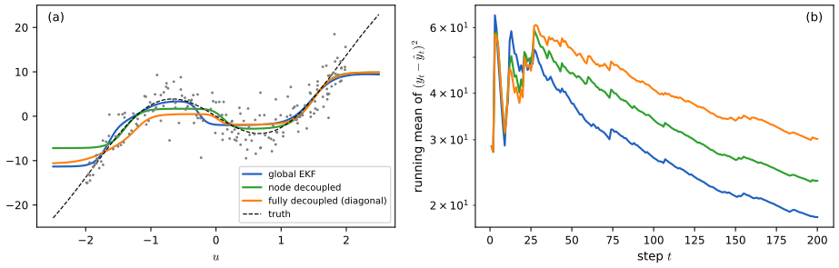
fig_17_S8, ekf_mlp (argument groups). Download: PDF · SVG17.5.3 Assumed density filtering for DNNs
pp. 675–676, (17.45)–(17.52) The EKF linearises the network; assumed density filtering (ADF; Section 8.6.3 for logistic regression, notes on ADF for DNNs) instead propagates Gaussian moments through the layers (Gaussian moment matching of the hidden activations). The likelihood is \[ p(y_t\given\bm u_t,\bm w_t)=\mathrm{Expfam}(y_t\given\ell^{-1}(f(\bm u_t;\bm w_t))) \] (17.45), for instance \(\mathrm{Ber}(y_t\given\sigma(\bm u_t^\T\bm w_t))\) (17.46) for a linear \(f\). Probabilistic backpropagation (PBP; Hernández-Lobato and Adams 2015) approximates the posterior of the weights by a fully factorised Gaussian
\[ p(\bm w_t\given\mathcal D_{1:t})\approx p_t(\bm w_t)=\prod_{l=1}^L\prod_{i=1}^{D_l}\prod_{j=1}^{D_{l-1}+1}\N(w_{ijl}\given\mu^t_{ijl},\tau^t_{ijl}) \tag{17.47}\](\(L\) layers, \(D_l\) neurons in layer \(l\); expectation backpropagation, Soudry et al. 2014, fixes the variances \(\tau=1\)). For static parameters the new posterior after the \(t\)-th observation is \[ \hat p_t(\bm w)=\frac1{Z_t}p(y_t\given\bm u_t,\bm w)\N(\bm w\given\bm\mu_{t-1},\bm\Sigma_{t-1}) \] (17.48) with \(\bm\Sigma_{t-1}=\diag(\bm\tau^{t-1})\), and it is projected onto factored Gaussians by matching moments (Minka 2001):
\[ \mu^t_{ijl}=\mu^{t-1}_{ijl}+\tau^{t-1}_{ijl}\frac{\partial\ln Z_t}{\partial\mu^{t-1}_{ijl}},\qquad \tau^t_{ijl}=\tau^{t-1}_{ijl}-(\tau^{t-1}_{ijl})^2\Big[\Big(\frac{\partial\ln Z_t}{\partial\mu^{t-1}_{ijl}}\Big)^2-2\frac{\partial\ln Z_t}{\partial\tau^{t-1}_{ijl}}\Big]. \tag{17.49, 17.50}\]The forward pass propagates \(\bm u_t\) through the model with Gaussian weights; for some activations (ReLU) the integrals for the moments of the hidden units are analytic, as in GP-neural networks (Section 18.7), so the output pre-activation is \(\N(\eta_t\given\mu,\Sigma)\) and \[ Z_t\approx\int p(y_t\given\eta_t)\N(\eta_t\given\mu,\Sigma)\d\eta_t \] (17.51). For probit classification with \(y\in\{-1,+1\}\) and \(p(y\given\bm x,\bm w)=\Phi(y\eta)\), \[ \int\Phi(y\eta)\N(\eta\given\mu,\sigma)\d\eta=\Phi(y\mu/\sqrt{1+\sigma}) \] (17.52); for logistic classification the probit approximation of Section 15.3.6 is used, and for multiclass problems a variational lower bound on \(\log Z_t\) (Gal et al. 2016 is cited for it). Gradients of \(\ln Z_t\) (by backpropagation) then update the moments.
Filling the gap 17.26: the moment-matching formulas (17.49)–(17.50) p. 676
The book attributes the formulas to Minka (2001) and uses them. They follow from differentiating the normaliser with respect to the parameters of the Gaussian.
Derivation
Fix one weight \(w\) with prior \(\N(w\given\mu,\tau)\) (the others integrated out; the update of each weight uses the same formulas with \(Z\) a function of all moments) and write \(Z(\mu,\tau)=\int\ell(w)\N(w\given\mu,\tau)\d w\), where \(\ell(w)\) is the likelihood (as a function of this weight, with the rest averaged). The tilted distribution is \(\hat p(w)=\ell(w)\N(w\given\mu,\tau)/Z\) and ADF sets the new Gaussian to have the mean and variance of \(\hat p\).
Mean. \[ \partial_\mu\N(w\given\mu,\tau)=\frac{w-\mu}\tau\N(w\given\mu,\tau) \], so \[ \partial_\mu Z=\frac1\tau\int\ell(w)(w-\mu)\N\d w=\frac Z\tau(\E_{\hat p}[w]-\mu) \]. Hence \[ \E_{\hat p}[w]=\mu+\tau\,\partial_\mu\ln Z. \]
Variance. \[ \partial_\tau\N(w\given\mu,\tau)=\big(\frac{(w-\mu)^2}{2\tau^2}-\frac1{2\tau}\big)\N(w\given\mu,\tau) \], so \[ \partial_\tau Z=\frac Z{2\tau^2}\big(\E_{\hat p}[(w-\mu)^2]-\tau\big) \], i.e. \(\E_{\hat p}[(w-\mu)^2]=\tau+2\tau^2\partial_\tau\ln Z\). Then \[ \var_{\hat p}(w)=\E_{\hat p}[(w-\mu)^2]-(\E_{\hat p}[w]-\mu)^2=\tau+2\tau^2\partial_\tau\ln Z-\tau^2(\partial_\mu\ln Z)^2=\tau-\tau^2\big[(\partial_\mu\ln Z)^2-2\,\partial_\tau\ln Z\big]. \] Both are exactly (17.49) and (17.50) (with \(\tau\) a variance). The identities hold for any likelihood for which the integrals exist; for the probit model with \(\bm w\sim\N(\bm\mu,\diag\bm\tau)\) one has \(\eta=\bm w^\T\bm x\sim\N(\bm\mu^\T\bm x,v)\), \(v=\sum_i\tau_ix_i^2\), so by (17.52) \(Z=\Phi(a)\), \(a=y\bm\mu^\T\bm x/\sqrt{1+v}\), and \[ \partial_{\mu_i}\ln Z=\frac{y\,x_i}{\sqrt{1+v}}\frac{\N(a)}{\Phi(a)} \]: the familiar ADF update of online probit regression (Section 8.6.3). Because the update only involves the moments of the single factor \(\hat p\), ADF is the first pass of expectation propagation, with no iteration to refine earlier factors. A numerical experiment compared the formulas with moments of the tilted distribution obtained by quadrature.
See also: ADF for online logistic regression and for DNNs: Section 8.6.3, 8.6.4; the Chapter 10 notes on EP: Section 10.7.
17.5.4 Online variational inference for DNNs
pp. 676–677, (17.53)–(17.56) Variational inference can be run online with the previous posterior as the prior: streaming variational Bayes (Broderick et al. 2013). At step \(t\)
\[ \bm\psi_t=\argmin_{\bm\psi}\ \E_{q(\th\given\bm\psi)}[\ell_t(\th)]+\KL\big(q(\th\given\bm\psi)\,\|\,q(\th\given\bm\psi_{t-1})\big)=\argmin_{\bm\psi}\E_{q(\th\given\bm\psi)}\big[\ell_t(\th)+\log q(\th\given\bm\psi)-\log q(\th\given\bm\psi_{t-1})\big], \tag{17.53, 17.54}\]with \(\ell_t(\th)=-\log p(\mathcal D_t\given\th)\) (or another loss) the loss of the \(t\)-th batch, minimised over \(\bm\psi\) (the negative of the quantity written \(\ELBO_t(\bm\psi)\)). For DNNs this is variational continual learning (VCL; Nguyen et al. 2018; an efficient version is FOO-VB, Zeno et al. 2021). A problem is variational overpruning (Trippe and Turner 2017): weights not needed to fit the current data keep their prior posterior, sampling them adds noise to the likelihood, and the optimiser reduces that noise by driving the bias to a large negative value, switching the unit off; such "dead units" stay stuck and the network lacks the capacity for the next task. Generalised VCL (GVCL; Loo et al. 2021) first down-weights the KL term by \(\beta<1\), and then tempers prior and posterior,
\[ \ELBO_t=\E_{q(\th\given\bm\psi)}[\ell_t(\th)]+\beta\,\KL\big(q(\th\given\bm\psi)\,\|\,q(\th\given\bm\psi_{t-1})\big),\qquad \ELBO^{\lambda}_t=\E_{q}[\ell_t(\th)]+\beta\,\KL\big(q^{\lambda}\,\|\,(q_{t-1})^{\lambda}\big), \tag{17.55, 17.56}\](the printed version of (17.56) has lost the arguments of the KL; the sense is that the Gaussians are raised to the power \(\lambda\), i.e. their covariances are scaled by \(\lambda^{-1}\), temperature \(\tau=1/\lambda\)), optimised by SGD when \(q\) is reparameterisable. In the limit \(\beta\to0\) GVCL recovers methods based on Laplace approximations: with a diagonal Gaussian it gives online EWC (Schwarz et al. 2018), with a block-diagonal Kronecker-factored one the online structured Laplace method of Ritter et al. (2018), and with a low-rank precision the SOLA method of Yin et al. (2020).
Filling the gap 17.27: why VCL is Bayes' rule in variational form, and the \(\beta\to0\) limit pp. 676–677
The book says "one can show" that GVCL tends to Laplace methods as \(\beta\to0\). Here is the derivation for Gaussians.
Derivation
(17.53)–(17.54). Bayes' rule is \[ p(\th\given\mathcal D_{1:t})=p(\mathcal D_t\given\th)q_{t-1}(\th)/Z_t \] with \(q_{t-1}\) the previous approximation. For any \(q\), \[ \KL(q\,\|\,p(\cdot\given\mathcal D_{1:t}))=\E_q[\log q-\log q_{t-1}-\log p(\mathcal D_t\given\th)]+\log Z_t \], so minimising it over \(q\) is minimising \(\E_q[\ell_t+\log q-\log q_{t-1}]\) with \(\ell_t=-\log p(\mathcal D_t\given\th)\), which is (17.54), and the term \(\E_q[\log q-\log q_{t-1}]=\KL(q\,\|\,q_{t-1})\) gives (17.53).
The limit. Let \(q=\N(\bm\mu,\bm\Sigma)\), \(q_{t-1}=\N(\bm\mu_0,\bm\Lambda_0^{-1})\) and expand the loss to second order about \(\bm\mu\): \[ \E_q\ell_t\approx\ell_t(\bm\mu)+\frac12\Tr(\bm H_t\bm\Sigma) \] with \(\bm H_t\) the Hessian of \(\ell_t\). With \[ \KL=\frac12[\Tr(\bm\Lambda_0\bm\Sigma)+(\bm\mu-\bm\mu_0)^\T\bm\Lambda_0(\bm\mu-\bm\mu_0)-P-\log|\bm\Lambda_0\bm\Sigma|] \], the objective \(\ell_t(\bm\mu)+\frac12\Tr(\bm H_t\bm\Sigma)+\beta\KL\) is stationary in \(\bm\Sigma\) when \[ \frac12\bm H_t+\frac\beta2(\bm\Lambda_0-\bm\Sigma^{-1})=\bm0 \], that is \[ \bm\Sigma^{-1}=\bm\Lambda_0+\frac1\beta\bm H_t,\qquad\bm\Sigma=\beta(\beta\bm\Lambda_0+\bm H_t)^{-1}. \] With \(\lambda=1/\beta\) this is \(\bm\Lambda_t=\bm\Lambda_{t-1}+\lambda\bm H_t\), exactly (17.40). For the mean, \[ \nabla\ell_t(\bm\mu)+\beta\bm\Lambda_0(\bm\mu-\bm\mu_0)=\bm0 \] (plus a term \(\frac12\Tr(\nabla\bm H_t\bm\Sigma)\) from the third derivative, which is \(O(\beta)\)), i.e. \(\bm\mu\) minimises \(\lambda\ell_t(\bm\mu)+\frac12(\bm\mu-\bm\mu_0)^\T\bm\Lambda_0(\bm\mu-\bm\mu_0)\): the weighted sequential Laplace step (17.39) with the data weighted by \(\lambda\). Since \(\bm\Sigma=O(\beta)\) the quadratic expansion of the loss is accurate as \(\beta\to0\): the second-order approximation becomes exact, and GVCL with a Gaussian family is the sequential Laplace/EWC recursion of Filling the gap 17.22, with the family fixing the structure of \(\bm\Lambda\) (diagonal: EWC; Kronecker-factored: structured Laplace). For a quadratic \(\ell_t\) the formulas are exact for every \(\beta\), and a direct numerical minimisation of the objective agreed with them. The role of \(\beta<1\) against variational overpruning is visible here: it divides the prior's pull by \(\beta\) relative to the data's, weakening the incentive to match the old posterior in directions the new data do not need.
17.6 Hierarchical Bayesian neural networks
pp. 677–678 When several related data sets are available (images from different hospitals), some aspects are shared and others are specific. A hierarchical Bayesian model lets each data set have its own parameters (random effects) drawn from a common prior (shared effects), as in the hierarchical GLMs of Section 15.5; the setting resembles domain generalisation (Section 19.6.2) except that we care about all the domains, not a held-out one.
17.6.1 Example: multimoons classification
pp. 678–680, (17.57), Figures 17.17–17.19 Solve \(J=18\) related nonlinear binary classification problems, each with its own boundary \(p(y\given\bm x,\bm w_j)\), similar to a common boundary \(p(y\given\bm x,\bm w_0)\) (concept shift, Section 19.2.3), with few examples (\(N_j=50\)) each. The data are the two-moons set rotated by a different amount for each task (Figure 17.17). Fitting separate MLPs works poorly (little data per task) and pooling all data does worse (different concepts). In the hierarchical model (Figure 17.18) the weight from unit \(i\) to unit \(k\) in layer \(l\) for task \(j\) is a common value plus a random offset, in the non-centred parameterisation of Section 12.6.5,
\[ w^j_{i,k,l}=w^0_{i,k,l}+\epsilon^j_{i,k,l}\,\sigma^0_l,\qquad\epsilon^j_{i,k,l}\sim\N(0,1), \tag{17.57}\]with a separate \(\sigma^0_l\) per layer so that the model controls the shrinkage to the prior layer by layer (the \(\sigma_l\) could also be task specific). The hyperpriors are \(\N(0,1)\) on \(w^0_{i,k,l}\) and \(\N^+(1)\) (half normal) on \(\sigma^0_l\). The posterior \(p(\bm\epsilon,\bm w^0,\bm\sigma^0\given\mathcal D)\) is computed by HMC (Section 12.5) and the model is evaluated on fresh data from each task; the book reports average accuracies of 86% (train) and 83% (test) for the separate models against 91% and 89% for the hierarchical one. Figure 17.19 shows why: the separate models fail to learn the common Z-shaped boundary, the hierarchical one recovers it while allowing group variation.
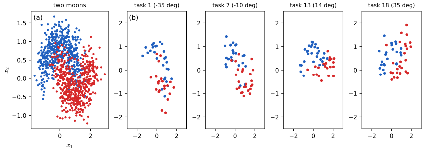
fig_17_17, multimoons. Reproduces Murphy (2023), Figure 17.17 (our own rotation angles). Download: PDF · SVGFilling the gap 17.28: partial pooling, in closed form, and the non-centred form (17.57) pp. 678–679
The book explains the benefit qualitatively. The linear-Gaussian version of (17.57) shows exactly how the group parameters are shrunk to the shared ones.
Derivation
Non-centred = centred. If \(\epsilon\sim\N(0,1)\) then \(w^0+\sigma^0\epsilon\sim\N(w^0,(\sigma^0)^2)\): (17.57) defines the same distribution of \(w^j\) as the centred form \(w^j\sim\N(w^0,(\sigma^0)^2)\); it differs only in the coordinates in which a sampler moves (and removes the funnel geometry between \(\sigma^0\) and \(\bm w^j\); Section 12.6.5).
Shrinkage. Suppose task \(j\) is a linear regression \(\bm y_j=\bm X_j\bm w_j+\bm\varepsilon_j\), noise variance \(\sigma^2\), with \(\bm w_j\sim\N(\bm w_0,\sigma_0^2\bm I)\). Given \((\bm w_0,\sigma_0)\) the posterior of \(\bm w_j\) is Gaussian with precision \(\bm\Lambda_j=\bm X_j^\T\bm X_j/\sigma^2+\bm I/\sigma_0^2\) and mean \[ \bm\Lambda_j^{-1}\Big(\frac{\bm X_j^\T\bm y_j}{\sigma^2}+\frac{\bm w_0}{\sigma_0^2}\Big)=(\bm I-\bm B_j)\hat{\bm w}_j+\bm B_j\bm w_0,\qquad\bm B_j=\Big(\bm I+\frac{\sigma_0^2}{\sigma^2}\bm X_j^\T\bm X_j\Big)^{-1}, \] where \(\hat{\bm w}_j=(\bm X_j^\T\bm X_j)^{-1}\bm X_j^\T\bm y_j\) is the task's least-squares fit (when it exists): a matrix-weighted average of the separate fit and the shared value. The eigenvalues of \(\bm B_j\) lie in \((0,1]\): directions that the task's data determine well (large eigenvalue of \(\bm X_j^\T\bm X_j\)) keep their own fit, directions that they do not are shrunk to \(\bm w_0\). As \(\sigma_0\to0\), \(\bm B_j\to\bm I\) (complete pooling: every task uses \(\bm w_0\)); as \(\sigma_0\to\infty\), \(\bm B_j\to\bm 0\) (separate fits). Learning \(\sigma_0^l\) per layer lets the data pick the amount of sharing per layer, which is the point of (17.57). With only 50 points per task and 51 weights, most directions are poorly determined and the shared prior carries most of the information, which is why the hierarchical network gains. A numerical experiment of the posterior mean formula agreed.
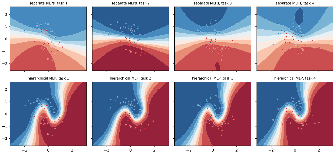
fig_17_19, hier_moons. Reproduces Murphy (2023), Figure 17.19 (the book reports 86/83 and 91/89). Download: PDF · SVGPractice problems
Chapter 17 of the book has no end-of-chapter exercises. Here are three short problems with worked solutions.
Problem 17.1 (the prior of a ReLU network grows linearly). A one-hidden-layer ReLU network with scalar input and output has \(H\) hidden units, \(W_1\sim\N(0,\alpha_1^2)\), \(W_2\sim\N(0,\alpha_2^2)\) and no biases. Find \(\var f(x)\) exactly and the distribution of \(f(x)/|x|\) for \(x\ne0\). For \(H=12\) and \(\alpha_1=\alpha_2=1\) what is the prior standard deviation at \(x=1\)?
Solution
By homogeneity \(f(x)=|x|\,f(\mathrm{sgn}(x))\), so \(f(x)/|x|\) has the same law for every \(x\ne0\) (the standard deviation grows linearly with \(|x|\)). At \(x=1\), \(f(1)=\sum_jW_{2j}\max(W_{1j},0)\); given \(W_1\) this is Gaussian with variance \(\alpha_2^2\sum_j\max(W_{1j},0)^2\), and \(\E\max(W_1,0)^2=\alpha_1^2/2\) (half of the mass, symmetric). Because the \(H\) terms are independent and centred, \(\var f(1)=H\alpha_2^2\alpha_1^2/2\), and \(\var f(x)=H\alpha_1^2\alpha_2^2x^2/2\). For \(H=12\), \(\alpha_1=\alpha_2=1\): \(\var f(1)=6\), standard deviation \(\sqrt6=2.449\). The distribution of \(f(1)\) is not Gaussian (a scale mixture of Gaussians with a chi-squared-like mixing variable), though it is for large \(H\) by the central limit theorem. A simulation of \(2\times10^5\) networks gave a standard deviation of 2.44 and the demonstration, with \(\alpha_1=1\), \(\alpha_2=1\), \(\beta=0\), \(H=12\) and ReLU, shows \(\sqrt6\) at \(x=1\).
Problem 17.2 (the Laplace bridge for two classes). For \(C=2\) take zero-sum logits \(\bm m=(\mu,-\mu)\) and covariance \(\bm V=s^2\bm I\) in (17.29) (ignore the optional rescaling). Show that the mean class probability \(\alpha_1/\alpha_0\) equals \(\sigma(2\mu)\), the sigmoid of the logit difference, and find the concentration \(\alpha_0\).
Solution
With \(C=2\), \(1-2/C=0\), so \(\alpha_i=\frac{e^{m_i}}{4s^2}\sum_je^{-m_j}\). Here \(\sum_je^{-m_j}=e^{-\mu}+e^{\mu}=2\cosh\mu\). Hence \[ \alpha_1=\frac{e^{\mu}\,2\cosh\mu}{4s^2}=\frac{e^\mu\cosh\mu}{2s^2} \] and \(\alpha_2=\frac{e^{-\mu}\cosh\mu}{2s^2}\). The mean probability is \[ \frac{\alpha_1}{\alpha_0}=\frac{e^\mu}{e^\mu+e^{-\mu}}=\sigma(2\mu) \], and \[ \alpha_0=\frac{\cosh\mu}{2s^2}(e^\mu+e^{-\mu})=\frac{\cosh^2\mu}{s^2} \]. So for two classes the bridge reproduces the plug-in probability \(\sigma(z_1-z_2)\) (the mean does not move towards 0.5 as the logit variance grows) and puts the uncertainty into the concentration \(\alpha_0=\cosh^2\mu/s^2\): larger logit variance \(s^2\) gives a smaller \(\alpha_0\), a more diffuse Beta distribution over \(\pi_1\). This was confirmed numerically for \(\mu=0.7\) and \(s^2=0.4\).
Problem 17.3 (tempering and the log loss). Observations \(y_i\sim\N(\theta,\sigma^2)\), a flat prior on \(\theta\), and the tempered posterior with power \(\alpha\) on the likelihood. For a new observation \(y_*\) the predictive is \(\N(\bar y,\sigma^2+\sigma^2/(\alpha N))\). Compute the expected log loss over data and \(y_*\) under the truth and show that it is minimised at \(\alpha=1\).
Solution
The tempered posterior is \(\N(\bar y,\sigma^2/(\alpha N))\) (the precision is \(\alpha N/\sigma^2\)), so the predictive has variance \(v_\alpha=\sigma^2(1+a)\) with \(a=1/(\alpha N)\). Under the truth, \(\bar y\sim\N(\theta_0,\sigma^2/N)\) and \(y_*\sim\N(\theta_0,\sigma^2)\) are independent, so \(\E(y_*-\bar y)^2=\sigma^2(1+1/N)\). The expected log loss is \[ \ell(\alpha)=\tfrac12\log(2\pi\sigma^2(1+a))+\frac{\sigma^2(1+1/N)}{2\sigma^2(1+a)}=\tfrac12\log(2\pi\sigma^2)+\tfrac12\log(1+a)+\tfrac12\frac{1+1/N}{1+a}. \] The derivative with respect to \(a\) is \(\frac1{2(1+a)}-\frac{1+1/N}{2(1+a)^2}\), zero at \(1+a=1+1/N\), i.e. \(a=1/N\), \(\alpha=1\); the second derivative is positive there, so it is a minimum. (This is Result 17.1(a) in a case that can be computed by hand: when the model is correct the exact posterior is optimal, and \(\alpha>1\) (cold) under-represents epistemic uncertainty, \(\alpha<1\) over-represents it.) A cold posterior can still help when the model is misspecified, as Section 17.3.11 explains. A Monte Carlo estimate with \(N=10\) confirmed \(\ell(1)<\ell(0.5)\) and \(\ell(1)<\ell(2)\) and the formula.
Demonstrations for this chapter
Each demonstration runs in the browser, with seeded random numbers so that a class sees the same pictures, and links back to these notes. The ▶ Demo boxes above open them already set to the case under discussion. The pages run the same algorithms as the Python code, with the same random-number generator for the draws, so their numbers are those of the code.
| Demonstration | What you can see | Sections and results |
|---|---|---|
| Priors over functions | Ten random functions from a Gaussian prior on a one-hidden-layer network, with the exact prior standard deviation, as the four scales, the width and the activation change. Presets: 1 Figure 17.1(a); 2 alpha1 = 25; 3 beta1 = 5; 4 alpha2 = 5; 5 ReLU without biases; 6 200 tanh units. | 17.2.1; Filling the gap 17.2; Problem 17.1 |
| Approximate posteriors against HMC | A one-dimensional regression with a gap: MAP, deep ensemble, MC dropout and two Laplace approximations against a long HMC run, with the standard deviation of the function at three inputs. Presets: 1 MAP; 2 ensemble; 3 MC dropout 0.1; 4 MC dropout 0.3; 5 Laplace, all weights; 6 Laplace, last layer. | 17.3.1, 17.3.2, 17.3.7, 17.3.9; Filling the gaps 17.4, 17.5, 17.9 |
| BMA under a shift | A network with an input that was constant in training: accuracy and log probability of the MAP and of the Bayesian average as the corruption of that input grows, for a wide or a narrow prior on its weights. Presets: 1 no corruption; 2 s = 3, prior sd 1; 3 s = 3, prior sd 0.05; 4 s = 6. | 17.4.6.1; Filling the gap 17.20; Figure 17.S5 |
The Python code that produces every figure of this page is code/ch17_bayesian_neural_networks.py (see the code index).
Errors and slips found in the book
Everything below was confirmed by recomputation or by the derivations above. Items marked (minor) are notational.
- (17.39): the quadratic penalty must use the precision \(\bm\Lambda_{t-1}\), not \(\bm\Lambda_{t-1}^{-1}\) (which is the covariance of the previous posterior, as the text just before (17.38) defines it); the transpose is also missing (Filling the gap 17.22).
- (17.43): \(h^\star(u)=x-10\cos(u)\sin(u)+u^3\) should read \(u-10\cos(u)\sin(u)+u^3\); with \(x\) undefined the example cannot be reproduced (Section 17.5.2.1).
- Supplement (17.11): \[ \bm S_k=\bm R_k+\sum_j(\bm H^j_k)^\T\bm\Sigma^j_{k|k-1}\bm H^j_k \] should be \(\bm R_k+\sum_j\bm H^j_k\bm\Sigma^j_{k|k-1}(\bm H^j_k)^\T\), the \(N\times N\) matrix; the printed product is \(M_j\times M_j\) (Filling the gap 17.24). Equation (17.16) of the supplement is empty (an alignment artefact).
- (17.26)–(17.28) and (17.16): the Jacobian is \(C\times P\) in (17.14)–(17.16) and \(P\times C\) in the text after (17.26); with the \(C\times P\) convention (17.28) should read \(\bm J\bm\Sigma\bm J^\T\), not \(\bm J^\T\bm\Sigma\bm J\) (Filling the gap 17.5).
- (17.52): \[ \int\Phi(y\eta)\N(\eta\given\mu,\sigma^2)\d\eta=\Phi(y\mu/\sqrt{1+\sigma^2}) \]: the book writes \(\sqrt{1+\sigma}\) with \(\sigma\) a variance and the integration variable as \(h\) in the density (Filling the gap 17.7).
- (17.53) and (17.55)–(17.56): the arguments of the KL divergence are missing in the draft (the underbrace label of (17.53) and the right-hand sides of (17.55), (17.56) are cut); the sense is \(\KL(q(\th\given\bm\psi)\,\|\,q(\th\given\bm\psi_{t-1}))\) and its tempered version (Section 17.5.4).
- (minor) Footnote 1 of Section 17.3.2: \(\nabla_f\|\bm y-\bm f\|^2=2(\bm f-\bm y)\) (a vector), not \(2\|\bm y-\bm f\|\). Sections 17.3.2 and 17.5.1: "posterior prediction matrix" should be "posterior precision matrix". (17.15): the last factor should be \(\bm J_\th(\bm x)\), not \(\bm J_\th(\th)\).
- (minor) Section 17.3.8: the low-rank SWAG covariance is written \(\frac1S\bm\Delta\bm\Delta^\T\) with \(\bm\Delta\) built from the last \(K\) deviations; the original SWAG paper normalises by \(K-1\), and the letter \(S\) is used for both the number of samples and \(K\). (17.10): the remark that \(\phi(\alpha z)=0\) for negative \(\alpha\) is unnecessary, since \(\alpha_\ell>0\) is a standard deviation (Filling the gap 17.2).
References
- Murphy, K. P. (2023). Probabilistic Machine Learning: Advanced Topics. MIT Press. Chapter 17 (pp. 647–680) and Supplementary Section 17.1. probml.github.io/pml-book/book2.html.
- Aitchison, L. (2021). A statistical theory of cold posteriors in deep neural networks. ICLR.
- Bissiri, P. G., Holmes, C. C. and Walker, S. G. (2016). A general framework for updating belief distributions. Journal of the Royal Statistical Society B, 78, 1103–1130.
- Blundell, C., Cornebise, J., Kavukcuoglu, K. and Wierstra, D. (2015). Weight uncertainty in neural networks. ICML.
- Dinh, L., Pascanu, R., Bengio, S. and Bengio, Y. (2017). Sharp minima can generalize for deep nets. ICML.
- Donsker, M. D. and Varadhan, S. R. S. (1975). Asymptotic evaluation of certain Markov process expectations for large time, I. Communications on Pure and Applied Mathematics, 28, 1–47.
- Feldkamp, L. A. and Puskorius, G. V. (1994). Training controllers for robustness: multi-stream DEKF. IEEE International Conference on Neural Networks.
- Gal, Y. and Ghahramani, Z. (2016). Dropout as a Bayesian approximation: representing model uncertainty in deep learning. ICML.
- Garipov, T., Izmailov, P., Podoprikhin, D., Vetrov, D. and Wilson, A. G. (2018). Loss surfaces, mode connectivity, and fast ensembling of DNNs. NeurIPS.
- Graves, A. (2011). Practical variational inference for neural networks. NeurIPS.
- He, B., Lakshminarayanan, B. and Teh, Y. W. (2020). Bayesian deep ensembles via the neural tangent kernel. NeurIPS.
- Hein, M., Andriushchenko, M. and Bitterwolf, J. (2019). Why ReLU networks yield high-confidence predictions far away from the training data and how to mitigate the problem. CVPR.
- Hernández-Lobato, J. M. and Adams, R. P. (2015). Probabilistic backpropagation for scalable learning of Bayesian neural networks. ICML.
- Hinton, G., Vinyals, O. and Dean, J. (2014). Distilling the knowledge in a neural network. NIPS Deep Learning Workshop.
- Hobbhahn, M., Kristiadi, A. and Hennig, P. (2022). Fast predictive uncertainty for classification with Bayesian deep networks. UAI.
- Hochreiter, S. and Schmidhuber, J. (1997). Flat minima. Neural Computation, 9, 1–42.
- Hoeffding, W. (1963). Probability inequalities for sums of bounded random variables. Journal of the American Statistical Association, 58, 13–30.
- Hron, J., Matthews, A. G. de G. and Ghahramani, Z. (2018). Variational Bayesian dropout: pitfalls and fixes. ICML.
- Immer, A., Bauer, M., Fortuin, V., Rätsch, G. and Khan, M. E. (2021). Scalable marginal likelihood estimation for model selection in deep learning. ICML.
- Immer, A., Korzepa, M. and Bauer, M. (2021). Improving predictions of Bayesian neural nets via local linearization. AISTATS.
- Izmailov, P., Podoprikhin, D., Garipov, T., Vetrov, D. and Wilson, A. G. (2018). Averaging weights leads to wider optima and better generalization. UAI.
- Izmailov, P., Vikram, S., Hoffman, M. D. and Wilson, A. G. (2021). What are Bayesian neural network posteriors really like? ICML.
- Izmailov, P., Nicholson, P., Lotfi, S. and Wilson, A. G. (2021). Dangers of Bayesian model averaging under covariate shift. NeurIPS.
- Kapoor, S., Maddox, W. J., Izmailov, P. and Wilson, A. G. (2022). On uncertainty, tempering, and data augmentation in Bayesian classification. NeurIPS.
- Kingma, D. P., Salimans, T. and Welling, M. (2015). Variational dropout and the local reparameterization trick. NeurIPS.
- Kirkpatrick, J. et al. (2017). Overcoming catastrophic forgetting in neural networks. Proceedings of the National Academy of Sciences, 114, 3521–3526.
- Kristiadi, A., Hein, M. and Hennig, P. (2020). Being Bayesian, even just a bit, fixes overconfidence in ReLU networks. ICML.
- Lakshminarayanan, B., Pritzel, A. and Blundell, C. (2017). Simple and scalable predictive uncertainty estimation using deep ensembles. NeurIPS.
- Liu, J. Z. et al. (2020). Simple and principled uncertainty estimation with deterministic deep learning via distance awareness. NeurIPS.
- Loo, N., Swaroop, S. and Turner, R. E. (2021). Generalized variational continual learning. ICLR.
- Lotfi, S., Izmailov, P., Benton, G., Goldblum, M. and Wilson, A. G. (2022). Bayesian model selection, the marginal likelihood, and generalization. ICML.
- MacKay, D. J. C. (1992). Bayesian interpolation. Neural Computation, 4, 415–447; and A practical Bayesian framework for backpropagation networks. Neural Computation, 4, 448–472.
- MacKay, D. J. C. (1998). Choice of basis for Laplace approximation. Machine Learning, 33, 77–86.
- Maddox, W. J., Izmailov, P., Garipov, T., Vetrov, D. and Wilson, A. G. (2019). A simple baseline for Bayesian uncertainty in deep learning. NeurIPS.
- Mandt, S., Hoffman, M. D. and Blei, D. M. (2017). Stochastic gradient descent as approximate Bayesian inference. Journal of Machine Learning Research, 18, 1–35.
- Maurer, A. (2004). A note on the PAC Bayesian theorem. Preprint.
- McAllester, D. A. (1999). PAC-Bayesian model averaging. COLT.
- Minka, T. P. (2001). A family of algorithms for approximate Bayesian inference. PhD thesis, MIT.
- Neal, R. M. (1996). Bayesian Learning for Neural Networks. Springer.
- Nguyen, C. V., Li, Y., Bui, T. D. and Turner, R. E. (2018). Variational continual learning. ICLR.
- Osband, I. (2016). Risk versus uncertainty in deep learning: Bayes, bootstrap and the dangers of dropout. NIPS Workshop on Bayesian Deep Learning.
- Osband, I., Aslanides, J. and Cassirer, A. (2018). Randomized prior functions for deep reinforcement learning. NeurIPS.
- Ovadia, Y. et al. (2019). Can you trust your model's uncertainty? Evaluating predictive uncertainty under dataset shift. NeurIPS.
- Puskorius, G. V. and Feldkamp, L. A. (2003). Parameter-based Kalman filter training: theory and implementation (the review cited by the book as PF03).
- Rahimi, A. and Recht, B. (2007). Random features for large-scale kernel machines. NIPS.
- Ritter, H., Botev, A. and Barber, D. (2018). A scalable Laplace approximation for neural networks. ICLR; and Online structured Laplace approximations for overcoming catastrophic forgetting. NeurIPS.
- Singhal, S. and Wu, L. (1989). Training multilayer perceptrons with the extended Kalman algorithm. NIPS.
- Smith, S. L. and Le, Q. V. (2018). A Bayesian perspective on generalization and stochastic gradient descent. ICLR.
- Wen, Y., Tran, D. and Ba, J. (2020). BatchEnsemble: an alternative approach to efficient ensemble and lifelong learning. ICLR.
- Wenzel, F. et al. (2020). How good is the Bayes posterior in deep neural networks really? ICML.
- Wilson, A. G. and Izmailov, P. (2020). Bayesian deep learning and a probabilistic perspective of generalization. NeurIPS.
- Zhang, C., Bengio, S., Hardt, M., Recht, B. and Vinyals, O. (2017). Understanding deep learning requires rethinking generalization. ICLR.
The numerical statements in the text (the prior standard deviations and the Cauchy fraction, the evidence fixed point, the dropout variance, the GGN and the linearised predictive, the local reparameterisation variances, the probit integral, the random-feature variance and the bi-Lipschitz bounds, the symmetry counts, the stationary SGD covariance and the SWA variance, randomize-then-optimise, the batch-ensemble identity, the Laplace bridge, tempering, the effective dimension, the PAC-Bayes bound, the ReLU growth along rays, sequential Laplace, the EKF identities, the ADF moments, the GVCL limit, the hierarchical shrinkage, and the practice problems) were confirmed numerically.