Graphical models
A graphical model writes a joint distribution as a product of small local pieces and reads the conditional independences of that distribution off a graph. This chapter covers the three families (directed graphs or Bayes nets, undirected graphs or Markov random fields, and conditional random fields), compares what each can and cannot express, and ends with extensions: factor graphs, sum-product networks, relational and logical models, and structural causal models. The notes fill in what the book leaves to the literature: the exact arithmetic of its worked examples, the learning equations, the critical couplings of the Ising and Potts models, how a Hopfield network fails, why restricted Boltzmann machines factorise, the Gaussian and mean-field computations, label bias, and why interventions and counterfactuals are different questions.
Ch. 1 Introduction Ch. 2 Probability Ch. 3 Statistics Ch. 4 Graphical models Ch. 5 Information theory Ch. 6 Optimisation Ch. 7 Inference algorithms Ch. 8 Gaussian filtering Ch. 9 Message passing Ch. 10 Variational inference Ch. 11 Monte Carlo Ch. 12 MCMC Ch. 13 Sequential Monte Carlo Ch. 14 Predictive models Ch. 15 GLMs Ch. 16 Deep networks Ch. 17 Bayesian neural networks Ch. 18 Gaussian processes Ch. 19 Beyond iid Ch. 20 Generative models Ch. 21 VAEs Ch. 22 Autoregressive models Ch. 23 Normalizing flows Ch. 24 Energy-based models Ch. 25 Diffusion models Ch. 26 GANs Ch. 27 Discovery methods Ch. 28 Latent factor models Ch. 29 State-space models Ch. 30 Graph learning Ch. 31 Nonparametric Bayes Ch. 32 Representation learning Ch. 33 Interpretability Ch. 34 Decision making Ch. 35 Reinforcement learning Ch. 36 Causality
How to read these notes
They follow the book. Sections carry the book's numbers (4.2, 4.3.5, ...) and displayed equations that appear in the book carry its equation numbers, e.g. \((4.17)\). Material from the online supplement is placed where it belongs and labelled (supplement). Equations without a number are steps the book skips.
Filling the gaps. Wherever the book states a result without proof, leaves a calculation to the reader or quotes the literature, an orange Filling the gap box (or a proof) gives the argument. Derivations start hidden: open one with its bar, or use the button below. Results already proved in full in the companion courses are stated and linked rather than repeated.
Figures and demonstrations. Every figure of the chapter that is computed from a model or a simulation is reproduced from scratch by the Python code; the hand-drawn diagrams are not redrawn. Figures named 4.S1 to 4.S5 are extra ones made for the gaps. The ▶ Demo boxes open an interactive demonstration already set to the case being discussed.
Main reference
K. P. Murphy, Probabilistic Machine Learning: Advanced Topics, MIT Press (2023; the December 2025 draft is followed), Chapter 4, pages 143–217, and Supplementary Chapter 4, pages 39–48 (book web page: probml.github.io/pml-book/book2.html). Section, equation, figure and exercise numbers refer to this book. Chapter 4 has no end-of-chapter exercises, so three short practice problems with solutions are added at the end.
The explanations, derivations, figures and code are my own; equations are cited by their numbers in the book.
Companion courses
This chapter overlaps with several finished courses on this site, and the proofs there are not repeated here:
- Directed and undirected graphical models in Bishop's notation, with full proofs of the d-separation theorem, the Markov blanket, Hammersley–Clifford, moralisation and perfect maps: Bayesian and Probabilistic ML, Chapter 8.
- Conditional independence, d-separation, Markov equivalence, interventions and the truncated factorisation: All of Statistics, Chapter 17; undirected graphs, Gaussian graphical models and partial correlation: Chapter 18; log-linear models and iterative proportional fitting: Chapter 19; causal inference: Chapter 16.
- EM, mean field and the forward–backward algorithm: Chapter 9, Chapter 10 and Chapter 13 of the same course; Murphy's first volume: maximum entropy and moment matching.
New here: the exact numbers of the worked examples and the errors found in them, the learning equations for incomplete data, noisy-OR, Haldane's map function, the critical couplings, the Hopfield and Boltzmann-machine analysis, the Gaussian MRF with a linear term (and a corrected AR(1) covariance), nonlinear Gaussian factors and INLA, pseudolikelihood, CRFs and label bias, unrolled undirected models, sum-product networks, Markov logic, and counterfactuals.
The chapter at a glance
- 4.2 A DAG factorises the joint into one conditional per node (Result 4.1); the exact arithmetic of the student and sprinkler networks, including a slip in the text (Filling the gap 4.1, 4.2); noisy-OR and Haldane (4.3, 4.4); Gaussian Bayes nets have sparse precision (Result 4.2); d-separation, explaining away, Berkson's paradox in closed form (4.6); learning CPTs from complete and incomplete data (Result 4.6, Filling the gap 4.7).
- 4.3 Gibbs distributions and Hammersley–Clifford (Result 4.7); Ising and Potts models and their critical couplings (Filling the gap 4.9); Hopfield capacity (4.10); RBMs (4.11, 4.12); Gaussian MRFs, with two corrections to the AR(1) example (Result 4.8); mean-field denoising (4.16); maximum likelihood is moment matching (Result 4.10) and pseudolikelihood is not always equal to it (4.18).
- 4.4–4.5 CRFs: gradient and algorithms (Result 4.11); neither directed nor undirected graphs are more expressive (Result 4.12); label bias (4.22); the VAR example (4.23).
- 4.6–4.7 Sum-product networks, relational models and Markov logic (4.24 to 4.26); seeing is not doing (Result 4.13) and doing is not imagining (Result 4.14).
Notation. \(\mathbf{x}=(x_1,\dots,x_{N_G})\) are the nodes of a graph \(G\); \(\pa(i)\), \(\ch(i)\), \(\nd(i)\), \(\mb(i)\) are the parents, children, non-descendants and Markov blanket of node \(i\); \(A\indep B\given C\) is conditional independence. Gaussians in information form have precision \(\bm\Lambda=\bm\Sigma^{-1}\) and \(\bm\eta=\bm\Lambda\bm\mu\).
Prerequisites. Chapters 2 and 3 of the book (exponential family, multivariate Gaussians), and the first volume's chapters on probability and information theory.
4.1 Introduction
p. 143 A probabilistic graphical model (PGM) defines a joint distribution on random variables through a graph whose nodes are the variables and whose missing edges encode conditional independence assumptions (Murphy, 2023, Section 4.1). Two principles do the work: factorisation (the joint is a product of local terms) and averaging (marginalising over what is unobserved). The graph can be directed, undirected or mixed.
4.2 Directed graphical models (Bayes nets)
p. 143 A directed PGM (DPGM, Bayes net, belief network) is built on a directed acyclic graph (DAG). The name "Bayesian" is misleading: a Bayes net is only a way of defining a distribution, and nothing in it is more subjective than any other probabilistic model.
See also (companion course): Section 8.1, Bayesian networks; All of Statistics, Chapter 17.
4.2.1 Representing the joint distribution
pp. 143–144, (4.1)–(4.2) The nodes of a DAG can be ordered so that parents precede children (a topological order). Relative to such an order the ordered Markov property says that each node is independent of its other predecessors given its parents,
\[ x_i\indep x_{\mathrm{pred}(i)\setminus\pa(i)}\given x_{\pa(i)}, \tag{4.1} \]and the joint is
\[ p(x_{1:N_G})=\prod_{i=1}^{N_G}p(x_i\given x_{\pa(i)}). \tag{4.2} \]Result 4.1 (the ordered Markov property is equivalent to the factorisation; parameter counts) p. 144, (4.1)–(4.2)
Let \(1,\dots,N_G\) be a topological order of a DAG. A distribution satisfies the ordered Markov property (4.1) if and only if it factorises as (4.2). With tabular conditional probability distributions (CPDs), node \(i\) with \(K_i\) states and parents of \(K_p\) states has \((K_i-1)\prod_{p\in\pa(i)}K_p\) free parameters, so the whole net has
\[ \sum_{i}(K_i-1)\prod_{p\in\pa(i)}K_p=O(N_GK^{N_P+1}) \]free parameters when every node has at most \(N_P\) parents and \(K\) states, against \(\prod_iK_i-1=O(K^{N_G})\) for an unstructured table.
Proof
(\(\Rightarrow\)) The chain rule gives \(p(x_{1:N_G})=\prod_ip(x_i\given x_{1:i-1})\) for any distribution, and (4.1) replaces each factor by \(p(x_i\given x_{\pa(i)})\) because \(x_i\) is independent of \(x_{\mathrm{pred}(i)\setminus\pa(i)}\) given \(x_{\pa(i)}\) and \(\mathrm{pred}(i)=\{1,\dots,i-1\}\). (\(\Leftarrow\)) Suppose (4.2) holds. Summing out \(x_{N_G}\) (a node with no children, since the order is topological), then \(x_{N_G-1}\), and so on, shows that the marginal of \(x_{1:i}\) is \(\prod_{j\le i}p(x_j\given x_{\pa(j)})\), because each summed-out CPD sums to one and does not appear in the other factors. Hence \[ p(x_i\given x_{1:i-1})=p(x_i\given x_{\pa(i)}) \], which is (4.1). The count: a row of a CPT is a probability vector on \(K_i\) states (\(K_i-1\) free numbers) and there is one row per joint parent state. ∎
The same statements are proved, with the normalisation of (4.2), in Result 8.2 and Result 8.4 of the companion course and Theorem 17.6 of All of Statistics. For the student network of Section 4.2.2.2 the count is \(1+1+8+2+3=15\) against \(2\cdot2\cdot3\cdot2\cdot2-1=47\); for a long chain with \(K\) states it is linear in the length.
4.2.2 Examples
4.2.2.1 Markov chains
pp. 144–145, (4.3)–(4.4) The chain \(x_1\to x_2\to\cdots\) has joint \(p(x_1)\prod_{t\ge2}p(x_t\given x_{t-1})\) (4.3), and the present is a sufficient statistic for the past: the past and future are independent given \(x_t\), by the ordered Markov property. An order-2 chain adds the edges \(x_{t-2}\to x_t\) (4.4); in the limit the DAG is complete and the graph encodes no independence. (Hidden Markov models and the Baum–Welch special case of Section 4.2.7.5 are in Chapter 13 of the companion course.) One slip: the second form of (4.3) is printed with \(p(x_t\given x_{1:t-1})\); the first-order model has \(p(x_t\given x_{t-1})\).
4.2.2.2 The "student" network
pp. 145–146, (4.5)–(4.7), Figure 4.2 Five discrete variables: difficulty \(D\) (easy/hard), intelligence \(I\) (low/high), grade \(G\) (A/B/C), SAT score \(S\) (bad/good) and letter \(L\) (bad/good), with the edges \(D\to G\), \(I\to G\), \(I\to S\), \(G\to L\). With the topological order \(I,D,G,S,L\) the chain rule (4.5) collapses to
\[ p(D,I,G,L,S)=p(L\given G)\,p(S\given I)\,p(G\given D,I)\,p(D)\,p(I). \tag{4.6} \]A CPT is a row-stochastic matrix \(\theta_{ijk}=p(x_i=k\given x_{\pa(i)}=j)\) (4.7). The tables of Figure 4.2 are:
| \(D\) | Easy | Hard | \(I\) | Low | High |
|---|---|---|---|---|---|
| 0.60 | 0.40 | 0.70 | 0.30 |
| \(p(G\given I,D)\) | A | B | C | \(p(S\given I)\) | Bad | Good | \(p(L\given G)\) | Bad | Good |
|---|---|---|---|---|---|---|---|---|---|
| Low, Easy | 0.30 | 0.40 | 0.30 | Low | 0.95 | 0.05 | A | 0.10 | 0.90 |
| Low, Hard | 0.05 | 0.25 | 0.70 | High | 0.20 | 0.80 | B | 0.40 | 0.60 |
| High, Easy | 0.90 | 0.08 | 0.02 | C | 0.99 | 0.01 | |||
| High, Hard | 0.50 | 0.30 | 0.20 |
Filling the gap 4.1: the student network by hand, and a slip in the text pp. 146, 155, Figure 4.8
The book quotes posterior probabilities for the student network without showing the arithmetic. Here they are, and one of the quoted numbers is attached to the wrong evidence.
Derivation
Observe \(G=C\). Summing the joint (4.6) over \(S\) and \(L\) (which give 1) leaves \(p(D,I,G=C)=p(D)p(I)p(C\given I,D)\):
\[ p(G=C)=0.7\cdot0.6\cdot0.3+0.7\cdot0.4\cdot0.7+0.3\cdot0.6\cdot0.02+0.3\cdot0.4\cdot0.2=0.3496. \]The terms with \(I=\)High add to \(0.0036+0.024=0.0276\) and those with \(D=\)Hard to \(0.4(0.49+0.06)=0.22\), so
\[ p(I=\text{High}\given G=C)=\tfrac{0.0276}{0.3496}=0.0789,\qquad p(D=\text{Hard}\given G=C)=\tfrac{0.22}{0.3496}=0.6293, \]the 0.08 and 0.63 of Figure 4.8(a). Now also observe \(S=\)Good. The extra factor \(p(S=\text{Good}\given I)\) is 0.05 for \(I=\)Low and 0.8 for High, so \[ p(G=C,S=\text{Good})=0.035\cdot0.46+0.24\cdot0.092=0.03818 \], where \(0.46=0.6\cdot0.3+0.4\cdot0.7\) and \(0.092=0.6\cdot0.02+0.4\cdot0.2\). Then
\[ p(I=\text{High}\given G=C,S=\text{Good})=\tfrac{0.02208}{0.03818}=0.5783,\qquad p(D=\text{Hard}\given G=C,S=\text{Good})=\tfrac{0.4(0.035\cdot0.7+0.24\cdot0.2)}{0.03818}=0.7596. \]The slip. Section 4.2.6.1 writes "\(p(D=\text{Hard}\given G=C)=0.76\)" for the second case, but 0.76 is the probability given both observations (Figure 4.8b); given \(G=C\) alone it is 0.63, as the same paragraph says one sentence earlier. The mechanism is the one the book describes: the good SAT score makes high intelligence likely, which explains the grade away from low intelligence and leaves the hard class as the remaining explanation. The demonstration reproduces all these numbers exactly.
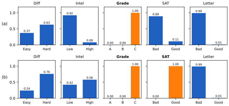
fig_4_8. Reproduces Murphy (2023), Figure 4.8. Download: PDF · SVG4.2.2.3 Sigmoid belief nets
p. 147, (4.8)–(4.10), Figure 4.3 A layered deep generative model \[ p(\mathbf{x},\mathbf{z})=p(\mathbf{z}_2)p(\mathbf{z}_1\given\mathbf{z}_2)p(\mathbf{x}\given\mathbf{z}_1) \] with binary hidden layers and logistic-regression CPDs \[ p(z_{\ell,k}=1\given\mathbf{z}_{\ell+1})=\sigma(\mathbf{w}_{\ell,k}^\T\mathbf{z}_{\ell+1}) \] is a sigmoid belief net (Neal, 1992); adding edges inside a layer gives a deep autoregressive network. Because the hidden units of one layer are parents of every unit below them, observing the bottom layer makes them dependent: the posterior over \(\mathbf{z}_1\) does not factorise (explaining away), in contrast with the undirected restricted Boltzmann machine of Section 4.3.3.2 (see Filling the gap 4.11).
Supplement 4.1: more examples of DGMs
Water sprinkler (supplement 4.1.1)
Supp. pp. 39–40, (4.1)–(4.2), Figure 4.1 Five binary variables: cloudy \(C\), sprinkler \(S\), rain \(R\), wet grass \(W\), slippery \(L\), with edges \(C\to S\), \(C\to R\), \(S\to W\), \(R\to W\), \(W\to L\). The joint is \[ p(C)p(S\given C)p(R\given C)p(W\given S,R)p(L\given W) \], where the supplement strikes out the conditioning variables that the graph makes unnecessary. It prints only the table of \(W\): \(p(W=1\given S,R)=0,0.9,0.9,0.99\) for \((S,R)=(0,0),(1,0),(0,1),(1,1)\).
Filling the gap 4.2: the sprinkler numbers 0.5, 0.7079 and 0.3204 Supp. p. 40
The supplement quotes \(p(R=1)=0.5\), \(p(R=1\given W=1)=0.7079\) and \(p(R=1\given W=1,S=1)=0.3204\) from code. The other tables are needed to reproduce them; the standard ones for this example are \(p(C=1)=0.5\), \(p(S=1\given C=0,1)=0.5,0.1\), \(p(R=1\given C=0,1)=0.2,0.8\), and they do give the quoted numbers (the table of \(L\) is not printed: the demonstration uses \(p(L=1\given W=0,1)=0,0.9\), our choice, which does not affect these probabilities).
Derivation
\(p(R=1)=0.5\cdot0.2+0.5\cdot0.8=0.5\). For the others, sum out \(C\) and \(S\). With \(R=1\) the factor for \(W=1\) is \(0.9\) if \(S=0\) and \(0.99\) if \(S=1\), so \[ p(W=1,R=1)=\sum_cp(c)p(R=1\given c)\big[p(S=0\given c)0.9+p(S=1\given c)0.99\big] \]:
\[ 0.5\cdot0.2\cdot0.945+0.5\cdot0.8\cdot0.909=0.4581. \]With \(R=0\) the factor is 0 for \(S=0\) and 0.9 for \(S=1\): \[ p(W=1,R=0)=0.5\cdot0.8\cdot0.45+0.5\cdot0.2\cdot0.09=0.189 \]. So \(p(R=1\given W=1)=0.4581/0.6471=0.7079\). Adding \(S=1\): \[ p(W=1,S=1,R=1)=0.99(0.5\cdot0.5\cdot0.2+0.5\cdot0.1\cdot0.8)=0.0891 \] and \[ p(W=1,S=1,R=0)=0.9(0.5\cdot0.5\cdot0.8+0.5\cdot0.1\cdot0.2)=0.189 \], whence \(0.0891/0.2781=0.3204\). Learning that the sprinkler was on explains the wet grass and lowers the probability of rain: explaining away again, now through a different collider (\(W\)).
Asia network (supplement 4.1.2)
Supp. pp. 40–41, Figure 4.2 The Asia network of Lauritzen and Spiegelhalter (1988) is a medical diagnosis example (visit to Asia, smoking, tuberculosis, lung cancer, bronchitis, X-ray, dyspnoea). The supplement shows only the marginals after each piece of evidence (dyspnoea present: cancer 5% to 10%, bronchitis 45% to 83%; then a visit to Asia: tuberculosis 2% to 9%; then smoking). The tables are not printed, so it is not recomputed here; it illustrates recursive Bayesian updating, which the demonstration lets you carry out on the student network.
The QMR network (supplement 4.1.3)
Supp. pp. 41–43, (4.3)–(4.6), Table 4.1 The quick medical reference (QMR) network is a bipartite DAG with hidden disease nodes \(z_k\) and visible symptom nodes \(x_d\), \[ p(\mathbf{z},\mathbf{x})=\prod_kp(z_k)\prod_dp(x_d\given\mathbf{z}_{\pa(d)}) \] (4.3). A symptom may have many parent diseases, so a CPT is too large; the noisy-OR model gives each parent link an independent chance to fail: \(\theta_{kd}=1-q_{kd}\) is the probability that the link \(k\to d\) fails. A leak node \(z_0\equiv1\) stands for all other causes, and (4.5) reads
\[ p(x_d=0\given\mathbf{z})=\theta_{0d}\prod_{k\in\pa(d)}\theta_{kd}^{z_k}. \tag{4.5} \]Filling the gap 4.3: noisy-OR as an OR of failing links, relation to logistic regression, and barren nodes Supp. pp. 42–43
The supplement states (4.4)–(4.6) and "barren node removal" without proof.
Derivation
Noisy-OR. Give each link from an active parent (including the leak) an independent Bernoulli variable \(u_{kd}\) with \(\Pr(u_{kd}=1)=q_{kd}\) ("the link works") and let \(x_d=\bigvee_{k:z_k=1}u_{kd}\). Then \(x_d=0\) iff every active link fails, which has probability \(\prod_{k:z_k=1}\theta_{kd}\), i.e. (4.5). Table 4.1 is the case of two diseases: the child is off with probability \(\theta_0\), \(\theta_0\theta_1\), \(\theta_0\theta_2\), \(\theta_0\theta_1\theta_2\) as the active set grows (confirmed numerically, together with a simulation of the failing links).
Relation to logistic regression. With \(w_{kd}=\log\theta_{kd}\le0\), (4.5) gives \[ p(x_d=1\given\mathbf{z})=1-\exp(w_{0d}+\sum_kz_kw_{kd}) \] (4.6). This has the same "linear score" but the link function is \(1-e^{-a}\) on \(a\le0\) instead of the sigmoid; it saturates at 1 only as all scores go to \(-\infty\), and a single parent active already gives the "causal power" \(q_{kd}\). The parameter count is linear in the number of parents, against \(2^{|\pa(d)|}\) for a CPT.
Barren nodes. An unobserved node with no observed descendants is barren: summing it out gives \(\sum_{x}p(x\given\mathbf{x}_{\pa})=1\), so its factor drops out of the joint over the other nodes. Hence unobserved symptoms can be deleted from the network before inference (assuming they are missing at random), which is how QMR keeps the cost proportional to the findings reported.
Genetic linkage analysis (supplement 4.1.4)
Supp. pp. 43–46, (4.7), Tables 4.2, Figures 4.4–4.5 For each person \(i\) and locus \(j\) the model has an observed phenotype \(P_{ij}\), hidden maternal and paternal alleles \(G^m_{ij},G^p_{ij}\) and hidden switching variables \(S^m_{ij},S^p_{ij}\). The penetrance model \(p(P\given G^m,G^p)\) maps genotypes to phenotypes (Table 4.2 is the many-to-one map from the ABO genotypes to blood types), the inheritance model (4.7) copies one of the parent's two alleles according to the switch, and the recombination model makes consecutive switches a two-state Markov chain that flips with probability \(\theta_j=\tfrac12(1-e^{-2d_j})\) at map distance \(d_j\).
Filling the gap 4.4: Haldane's recombination probability Supp. p. 45
The flip probability \(\theta=\tfrac12(1-e^{-2d})\) is quoted without derivation.
Derivation
Model crossovers along a chromosome as a Poisson process with rate 1 per Morgan (the definition of the map distance: one crossover expected per Morgan). Over a distance \(d\) the number of crossovers \(M\sim\mathrm{Poisson}(d)\). The inherited allele comes from the other grand-parental chromosome iff \(M\) is odd, so the switch flips with probability
\[ \Pr(M\text{ odd})=e^{-d}\sum_{m\text{ odd}}\frac{d^m}{m!}=e^{-d}\sinh d=\tfrac12\big(1-e^{-2d}\big). \]For small \(d\) this is \(\approx d\), so map distance and recombination fraction agree for close loci, and \(\theta\to\tfrac12\) (independent inheritance) for distant ones. Parities of crossovers over adjacent intervals are independent, so for adjacent distances \(d_1,d_2\), \[ \theta(d_1+d_2)=\theta_1(1-\theta_2)+\theta_2(1-\theta_1)=\theta_1+\theta_2-2\theta_1\theta_2 \]: the composition rule that makes the Markov-chain model of the switches consistent however the markers are subdivided. Both statements were checked by simulation and algebra.
The linkage likelihood needs the hidden \(S\) and \(G\) summed out, which is exact by variable elimination for small pedigrees and intractable for large ones (Chapter 9 of the book).
4.2.3 Gaussian Bayes nets
p. 148, (4.11)–(4.16) If every CPD is linear-Gaussian, \[ p(x_i\given x_{\pa(i)})=\N(x_i\given\mu_i+\mathbf{w}_i^\T x_{\pa(i)},\sigma_i^2) \] (4.11), the joint is a multivariate Gaussian (a directed Gaussian graphical model). Writing each node relative to its parents' means,
\[ x_i=\mu_i+\sum_{j\in\pa(i)}w_{ij}(x_j-\mu_j)+\sigma_iz_i,\quad z_i\sim\N(0,1), \tag{4.12} \]or \[ \mathbf{x}-\bm\mu=\mathbf{W}(\mathbf{x}-\bm\mu)+\mathbf{S}\mathbf{z} \] with \(\mathbf{W}\) strictly lower triangular in a topological order and \(\mathbf{S}=\diag(\sigma_i)\) (4.13)–(4.14).
Result 4.2 (moments and precision of a Gaussian Bayes net) p. 148, (4.15)–(4.16)
With \(\mathbf{U}=(\mathbf{I}-\mathbf{W})^{-1}\), \(\mathbf{x}\sim\N(\bm\mu,\bm\Sigma)\) with
\[ \bm\Sigma=\mathbf{U}\mathbf{S}^2\mathbf{U}^\T, \tag{4.16} \] \[ \bm\Lambda=\bm\Sigma^{-1}=(\mathbf{I}-\mathbf{W})^\T\mathbf{S}^{-2}(\mathbf{I}-\mathbf{W})=\sum_i\frac{1}{\sigma_i^2}(\mathbf{e}_i-\mathbf{w}_i)(\mathbf{e}_i-\mathbf{w}_i)^\T, \]where \(\mathbf{w}_i\) is the \(i\)th row of \(\mathbf{W}\) as a column. So \(\Lambda_{jk}\ne0\) only if \(j,k\) lie in a common family \(\{i\}\cup\pa(i)\): the sparsity pattern of the precision matrix is the moral graph (for generic weights), while \(\bm\Sigma\) is typically dense.
Proof
\(\mathbf{I}-\mathbf{W}\) is lower triangular with unit diagonal, so it is invertible and \[ \mathbf{x}-\bm\mu=\mathbf{U}\mathbf{S}\mathbf{z} \] is a linear map of a standard normal vector: Gaussian with mean \(\bm\mu\) (the \(\mathbf{z}\) have mean 0) and covariance \[ \mathbf{U}\mathbf{S}\mathbf{I}\mathbf{S}\mathbf{U}^\T \]. Inverting, \[ \bm\Sigma^{-1}=\mathbf{U}^{-\T}\mathbf{S}^{-2}\mathbf{U}^{-1}=(\mathbf{I}-\mathbf{W})^\T\mathbf{S}^{-2}(\mathbf{I}-\mathbf{W}) \]. Row \(i\) of \(\mathbf{I}-\mathbf{W}\) is \((\mathbf{e}_i-\mathbf{w}_i)^\T\), which is supported on \(\{i\}\cup\pa(i)\); the sum of rank-one terms follows, and each term contributes to the entries \((j,k)\) with \(j,k\in\{i\}\cup\pa(i)\), which is the family clique, joining every pair of parents of \(i\) (the "marriage"). Zeros can be created by cancellation for special weights, which is why the statement is for generic weights. The footnote of the book is also easy to see: if the parents' means are not subtracted, \(x_i=\mu_i+\sum_jw_{ij}x_j+\sigma_iz_i\) gives \[ \mathbb{E}[\mathbf{x}]=(\mathbf{I}-\mathbf{W})^{-1}\bm\mu \] and the same \(\bm\Sigma\). ∎
The companion course proves the same statement in Result 8.5. The precision formula is what the next sections use: it shows that a DAG on Gaussians and an undirected Gaussian model are two parameterisations of the same family (Section 4.5.5). Reproduced numerically: the covariance from 300,000 ancestral samples agrees with \(\mathbf{U}\mathbf{S}^2\mathbf{U}^\T\), the precision is its inverse, and the non-zero pattern is the moral graph.
4.2.4 Conditional independence properties
p. 149 Write \(X_A\indep_GX_B\given X_C\) when the graph \(G\) implies the independence, \(I(G)\) for the set of all such statements and \(I(p)\) for those true of a distribution \(p\). \(G\) is an I-map of \(p\) (\(p\) is Markov with respect to \(G\)) if \(I(G)\subseteq I(p)\); the complete graph is an I-map of every distribution; \(G\) is a minimal I-map if no subgraph is. It is a perfect map if \(I(G)=I(p)\) (Section 4.5.1).
4.2.4.1 Global Markov properties (d-separation)
pp. 149–151, (4.17)–(4.24), Figures 4.4–4.5, Table 4.1 A path is d-separated by \(C\) if it contains a chain \(s\to m\to t\) or \(s\leftarrow m\leftarrow t\) or a fork \(s\leftarrow m\to t\) with \(m\in C\), or a collider \(s\to m\leftarrow t\) such that neither \(m\) nor any descendant of \(m\) is in \(C\). \(A\) and \(B\) are d-separated by \(C\) if every path from \(A\) to \(B\) is, and then \(X_A\indep_GX_B\given X_C\) (4.17). The three elementary cases are proved in (4.18)–(4.24): conditioning on the middle of a chain or on the root of a fork separates the ends, while conditioning on the child of a collider links the parents. The Bayes ball algorithm (Shachter, 1998) is a way of checking this by bouncing balls along the graph.
Result 4.3 (the d-separation theorem) p. 149, (4.17)
Let \(G\) be a DAG and \(A,B,C\) disjoint node sets. (a) Soundness. If \(C\) d-separates \(A\) from \(B\), then \(X_A\indep X_B\given X_C\) for every distribution that factorises as (4.2). (b) Equivalent test. \(C\) d-separates \(A\) from \(B\) in \(G\) iff \(C\) separates \(A\) from \(B\) in the moralised ancestral graph \((G_{\mathrm{An}(A\cup B\cup C)})^m\) (Section 4.3.6.2). (c) Completeness (generic). If \(C\) does not d-separate \(A\) from \(B\), then for generic CPDs \(X_A\nindep X_B\given X_C\).
Proofs are in Result 8.9 of the companion course and Theorem 17.10 of All of Statistics; the part (b) is what makes the undirected route of Section 4.3.6.2 work, and its idea is the proof of soundness: the marginal on an ancestral set factorises over the families, each family is a clique of the moral graph, and factorisation over cliques implies the global Markov property of the undirected graph. In the code the two tests, a direct reachability search over (node, direction) pairs and the moral-ancestral test, are implemented independently; they agree on 1,500 random queries on random DAGs; for random CPTs every d-separated query has mutual information equal to zero to rounding error, and every non-d-separated one is strictly positive (part (c)). Table 4.1 of the book lists ten independences of the student network; all ten are d-separation statements and have exactly zero mutual information in the network (and the DAG implies 25 statements of the form \(x\indep y\given Z\) with single nodes \(x,y\) in all).
Filling the gap 4.5: the boundary conditions of Bayes ball p. 151, Figure 4.5
The book adds "boundary conditions": a ball hitting a hidden leaf stops, but one hitting an observed leaf bounces back. These are not extra rules: they are the collider rule applied to a descendant.
Derivation
Let \(Y'\) be a (possibly noisy) child of \(Y\) in the v-structure \(X\to Y\leftarrow Z\) with \(Y\to Y'\). The path \(X\to Y\leftarrow Z\) has \(Y\) as a collider, which is open iff \(Y\) or one of its descendants is observed. If \(Y'\) is observed, \(Y\) has an observed descendant, so the path is open: \(X\) and \(Z\) are dependent given \(Y'\). A ball sent down \(X\to Y\to Y'\) and bouncing back at \(Y'\) travels \(Y'\to Y\to Z\) and so reaches \(Z\). If \(Y'\) is hidden and a leaf it is barren; summing it out removes it without changing \(p(x,y,z)\), so no information passes. Quantitatively: with \(Y'=Y\oplus\) noise, observing \(Y'\) is a noisy observation of \(Y\), and by explaining away the posterior over \((X,Z)\) is \(\propto p(x)p(z)p(y'\given x,z)\), which does not factorise when \(p(y'\given x,z)\) depends on both.
4.2.4.2 Explaining away (Berkson's paradox)
pp. 151–153, (4.25), Figure 4.6 Conditioning on a common effect makes its causes dependent. The book's coin example: toss two coins 100 times and record the outcome only if at least one is heads. About 75 entries are recorded, and whenever coin 1 is tails coin 2 is heads, although the coins are independent: the recorded pairs are the pairs conditioned on a hidden common effect (the decision to record), which is selection bias. The Gaussian version is \(x\sim\N(-5,1)\), \(y\sim\N(5,1)\), \(z\given x,y\sim\N(x+y,1)\) (4.25), with the structure \(X\to Z\leftarrow Y\).
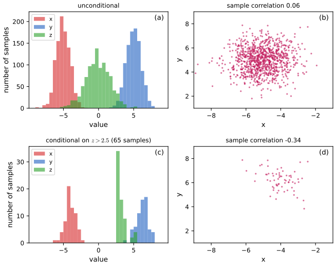
fig_4_6. Reproduces Murphy (2023), Figure 4.6. Download: PDF · SVGFilling the gap 4.6: Berkson's paradox in closed form p. 152, (4.25), Figure 4.6
The book shows samples. The induced correlation can be computed exactly, for conditioning on \(z\) and for selecting \(z>c\).
Derivation
Conditioning on \(z\). The joint of \((x,y,z)\) is Gaussian; in information form the posterior of \((x,y)\) given \(z\) has precision (prior precision \(\mathbf{I}\) plus the likelihood term \(\mathbf{1}\mathbf{1}^\T\) from \(z\given x,y\sim\N(x+y,1)\))
\[ \bm\Lambda_{xy\given z}=\begin{pmatrix}2&1\\1&2\end{pmatrix},\qquad \mathrm{Cov}(x,y\given z)=\tfrac13\begin{pmatrix}2&-1\\-1&2\end{pmatrix}, \]so \(\mathrm{corr}(x,y\given z)=-\tfrac12\) for every observed value of \(z\), and the conditional means are \(-5+z/3\) and \(5+z/3\) (\(\mathrm{Cov}(x,z)=1\), \(\mathrm{Var}(z)=3\)). Selecting \(z>c\). The law of total covariance with \(v=\mathrm{Var}(z\given z>c)\) (the variance of a \(\N(0,3)\) variable truncated to \((c,\infty)\)) gives
\[ \mathrm{Cov}(x,y\given z>c)=-\tfrac13+\tfrac{v}{9},\qquad \mathrm{Var}(x\given z>c)=\tfrac23+\tfrac{v}{9}, \]since the conditional means move with \(z\) at slope \(1/3\) each. With \(a=c/\sqrt3\) and the inverse Mills ratio \(\lambda=\varphi(a)/(1-\Phi(a))\), \(v=3(1+a\lambda-\lambda^2)\). For \(c=2.5\) this gives \(\mathrm{corr}=-0.3925\), selecting a fraction \(1-\Phi(2.5/\sqrt3)=0.0745\) of the samples, which is the 65 to 75 samples of Figure 4.6(c); a simulation of four million samples gives \(-0.391\). As \(c\to\infty\) the selected \(z\) concentrates, \(v\to0\) and \(\mathrm{corr}\to-\tfrac12\); for \(c\to-\infty\) it tends to \(0\). The unconditional correlation is 0, as the graph says (the collider is closed).
4.2.4.3 Markov blankets
pp. 153–154, (4.26)–(4.32), Figure 4.7 The Markov blanket of node \(i\) is the smallest set that renders \(i\) independent of all other nodes; in a DAG it is the parents, the children and the co-parents,
\[ \mb(i)=\ch(i)\cup\pa(i)\cup\mathrm{copa}(i), \tag{4.26} \]and the full conditional is proportional to the product of the family terms that contain \(x_i\),
\[ p(x_i\given x_{-i})=p(x_i\given x_{\mb(i)})\propto p(x_i\given x_{\pa(i)})\prod_{k\in\ch(i)}p(x_k\given x_{\pa(k)}). \tag{4.32} \]Result 4.4 (the Markov blanket of a DAG, with minimality) pp. 153–154, (4.26)–(4.32)
(4.32) holds, so \(x_i\indep x_{\text{rest}}\given x_{\mb(i)}\). Moreover no proper subset of \(\mb(i)\) has this property for generic distributions: if \(j\in\mb(i)\), then \(i\) and \(j\) are not d-separated by \(V\setminus\{i,j\}\).
Proof
The book's derivation (4.27)–(4.31) shows that all factors not involving \(x_i\) cancel between numerator and denominator, leaving (4.32). Minimality: let \(V\setminus\{i,j\}\) be observed. If \(j\) is a parent or a child of \(i\) the edge is an active path. If \(j\) is a co-parent, with common child \(k\), the path \(i\to k\leftarrow j\) has the collider \(k\) observed, so it is open. By Result 4.3(c) the dependence is present for generic CPDs; hence no element of \(\mb(i)\) can be dropped. ∎
Also proved in Result 8.10. Numerically, on random DAGs and CPTs, conditioning on the blanket leaves exactly zero mutual information with all other nodes, and (4.32) normalised reproduces the full conditional of the student network to \(10^{-18}\). The full conditionals are what the Gibbs sampler of Chapter 12 and the mean-field updates of Chapter 10 use.
4.2.4.4 Other Markov properties
pp. 153–154, (4.33)–(4.34), Figure 4.23 The local Markov property is \(i\indep\nd(i)\setminus\pa(i)\given\pa(i)\) (4.33), where \(\nd(i)\) are the non-descendants; the ordered property (4.34) is its restriction to predecessors in a topological order. The book states that the global (G), local (L), ordered (O) and factorisation (F) properties are equivalent and cites the literature.
Result 4.5 (the four directed Markov properties are equivalent) p. 154
For any distribution on the nodes of a DAG, \[ \mathrm{F}\Rightarrow\mathrm{G}\Rightarrow\mathrm{L}\Rightarrow\mathrm{O}\Rightarrow\mathrm{F} \], so all four hold or fail together.
Proof
\(\mathrm{F}\Rightarrow\mathrm{G}\) is soundness of d-separation (Result 4.3a). \(\mathrm{G}\Rightarrow\mathrm{L}\): \(\pa(i)\) d-separates \(i\) from \(\nd(i)\setminus\pa(i)\). Take a path from \(i\) to such a node \(v\). If its first edge points into \(i\), the first node after \(i\) is a parent \(p\in C=\pa(i)\); it is a non-collider on this path (the edge \(p\to i\) leaves \(p\)), so the path is blocked. If the first edge leaves \(i\), follow the path: if all its edges point forward it is a directed path \(i\to\cdots\to v\) and \(v\) would be a descendant, a contradiction; otherwise the first node where two arrows meet is a collider \(m\), which is a descendant of \(i\), and so are all its descendants; none lies in \(\pa(i)\) (a DAG has no cycles), so the collider is closed and the path is blocked. \(\mathrm{L}\Rightarrow\mathrm{O}\): \(\mathrm{pred}(i)\subseteq\nd(i)\) in a topological order, and independence of a bigger set implies independence of any subset (decomposition). \(\mathrm{O}\Rightarrow\mathrm{F}\) is the chain-rule argument of Result 4.1. ∎
This closes the cycle without citing Koller and Friedman (2009); it uses only soundness. For Figure 4.23(a) (reproduced in Section 4.3.6) the book's examples \(\nd(3)=\{1,2,4\}\), \(\pa(3)=\{1\}\), so \(3\indep\{2,4\}\given1\), and \(3\indep2\given1\) from the ordered property, are all confirmed by the code.
4.2.5 Generation (sampling)
p. 154 Visit the nodes in topological order and sample each from its CPD given the already sampled parents: ancestral sampling produces independent exact samples of (4.2). This is correct because the sample of \(x_{1:i}\) has the marginal \(\prod_{j\le i}p(x_j\given x_{\pa(j)})\) (the argument of Result 4.1), and each new draw is from the correct conditional. See Result 8.3.
4.2.6 Inference
p. 155, (4.35)–(4.37) Inference means computing the posterior of query nodes \(Q\) given visible nodes \(V\), marginalising over the nuisance nodes \(R\),
\[ p_\theta(Q\given V)=\frac{\sum_Rp_\theta(Q,V,R)}{p_\theta(V)}. \tag{4.35} \]In general this is NP-hard (Section 9.5.4), but chains, trees and sparse graphs admit dynamic programming (Chapter 9). Section 4.2.6.1 applies it to the student network, with the numbers of Filling the gap 4.1; here exact enumeration suffices.
4.2.6.1 Example: inference in the student network
Observing the grade C makes both explanations plausible, \(p(D=\text{Hard}\given C)=0.63\) and \(p(I=\text{High}\given C)=0.08\); also observing a good SAT score moves the probabilities to 0.76 and 0.58 (Figure 4.8, above). The demonstration lets you observe any subset and compare the d-separation verdict with the exact mutual information.
4.2.7 Learning
pp. 155–161, (4.38)–(4.62), Figures 4.9–4.10, Tables 4.2–4.3 With known structure \(G\) the task is parameter learning, computing the posterior \(p(\theta\given D)\) or a point estimate such as the MAP (structure learning is Section 30.3).
4.2.7.1 Learning from complete data
For a generative classifier with local variables \((x_n,y_n)\) and global parameters \(\theta_x,\theta_y\) (Figure 4.9), the CI structure gives \[ p(\theta,D)=[p(\theta_y)\prod_np(y_n\given\theta_y)][p(\theta_x)\prod_np(x_n\given y_n,\theta_x)] \] (4.38)–(4.40); in general \[ p(\theta,D)=\prod_ip(\theta_i)p(D_i\given\theta_i) \] (4.41), and the MLE decouples as \[ \hat\theta=\arg\max\prod_ip(D_i\given\theta_i) \] (4.42).
4.2.7.2 Example: computing the MLE for CPTs, and 4.2.7.3 computing the posterior for CPTs
Result 4.6 (learning tabular CPTs from complete data) pp. 157–159, (4.38)–(4.48), Tables 4.2–4.3
Let the data be complete and \(N_{ijk}=\sum_n\ind(x_{ni}=k,x_{n,\pa(i)}=j)\) (4.46). (a) The log-likelihood is \(\sum_{i,j,k}N_{ijk}\log\theta_{ijk}\), and its maximiser under the row constraints is \(\hat\theta_{ijk}=N_{ijk}/\sum_{k'}N_{ijk'}\) (4.47). (b) With independent priors \(\theta_{ij}\sim\mathrm{Dir}(\bm\alpha_{ij})\) on the rows, the posterior is a product of independent Dirichlets \[ \theta_{ij}\given D\sim\mathrm{Dir}(\mathbf{N}_{ij}+\bm\alpha_{ij}) \], with posterior mean \[ \bar\theta_{ijk}=(N_{ijk}+\alpha_{ijk})/\sum_{k'}(N_{ijk'}+\alpha_{ijk'}) \] (4.48); the MAP uses \(\alpha_{ijk}-1\) in place of \(\alpha_{ijk}\). (c) The marginal likelihood is \[ \prod_{i,j}\frac{\Gamma(\sum_k\alpha_{ijk})}{\Gamma(\sum_k\alpha_{ijk}+N_{ij})}\prod_k\frac{\Gamma(\alpha_{ijk}+N_{ijk})}{\Gamma(\alpha_{ijk})} \].
Proof
(a) The likelihood is a product over cases and nodes of \(\theta_{i,j(n),x_{ni}}\); collecting equal factors gives (4.44), \(\prod_{i,j,k}\theta_{ijk}^{N_{ijk}}\). The terms for different \((i,j)\) involve disjoint sets of parameters, so each row is maximised separately. For one row, maximise \(\sum_kN_k\log\theta_k\) subject to \(\sum_k\theta_k=1\): the Lagrangian \[ \sum_kN_k\log\theta_k+\lambda(1-\sum_k\theta_k) \] is stationary at \(\theta_k=N_k/\lambda\), and the constraint gives \(\lambda=\sum_kN_k\). The objective is concave (a sum of logarithms) and the constraint set is convex, so this is the global maximum on the simplex (rows with \(N_k=0\) give \(\hat\theta_k=0\)). (b) Prior times likelihood is \[ \prod_{ij}\prod_k\theta_{ijk}^{\alpha_{ijk}-1+N_{ijk}} \], a product of Dirichlet kernels with no coupling between rows, so the posterior factorises (this is (4.41): the graph has no path between the \(\theta_{ij}\) once all the \(x\) are observed). The Dirichlet mean is \(\alpha_k/\sum\alpha\) and its mode \((\alpha_k-1)/(\sum\alpha-K)\), giving (4.48) and the MAP statement. (c) Integrate each Dirichlet kernel with the normaliser \(\Gamma(\sum\alpha)/\prod\Gamma(\alpha_k)\). ∎
Dirichlet algebra is in Filling the gap 4.11 of the first volume's course; the tied-parameter and Bayesian chains are in Filling the gap 8.3. Table 4.3. From the seven training cases of Table 4.2 (columns \(I,D,G,S,L\)), the counts for \(G\) given \((I,D)\) are \([1,1,1]\) for (0,0), \([0,0,1]\) for (0,1), \([1,0,0]\) for (1,0) and \([0,1,1]\) for (1,1); so the MLE rows are \((\tfrac13,\tfrac13,\tfrac13)\), \((0,0,1)\), \((1,0,0)\), \((0,\tfrac12,\tfrac12)\), full of zeros, and the posterior means under a uniform Dirichlet(1,1,1) prior are \((\tfrac26,\tfrac26,\tfrac26)\), \((\tfrac14,\tfrac14,\tfrac24)\), \((\tfrac24,\tfrac14,\tfrac14)\), \((\tfrac15,\tfrac25,\tfrac25)\), exactly as the book prints; the zero-count problem is solved by the pseudo-counts. A check that the posterior really factorises: feeding the cases one at a time and multiplying the successive posterior-mean predictive probabilities of all the nodes gives the same number as the Dirichlet-multinomial formula (c), \(\log p(D)=-29.80\) for these seven cases.
4.2.7.4 Learning from incomplete data
pp. 159–160, (4.49)–(4.51), Figure 4.10 With a hidden node \(z_n\) in each case the likelihood is \[ \prod_n\sum_{z_n}p(z_n\given\theta_z)p(x_n\given z_n,\theta_x) \] and its logarithm (4.51) does not decompose over nodes: \(\log\) does not distribute over \(\sum_{z_n}\). In graph terms, \(\theta_z\to z_n\to x_n\leftarrow\theta_x\) has the observed collider \(x_n\), so the path between \(\theta_z\) and \(\theta_x\) is open and the posterior no longer factorises (footnote 2).
4.2.7.5 Using EM to fit CPTs, and 4.2.7.6 using SGD
Filling the gap 4.7: EM for CPTs and Fisher's identity pp. 160–161, (4.52)–(4.62)
The book describes the E step as returning "expected sufficient statistics" and states the SGD gradient (4.58)–(4.62). Here are the two derivations and the connection between them.
Derivation
EM. For tabular CPDs the complete-data log-likelihood is linear in the counts, \[ \log p(D_c\given\theta)=\sum_{ijk}N_{ijk}\log\theta_{ijk} \] (4.52). The EM auxiliary function is its expectation under the current posterior \(p(\mathbf{z}\given D,\theta^{\mathrm{old}})\); since the counts are sums of indicators, \[ \mathbb{E}[N_{ijk}]=\sum_np(x_{ni}=k,x_{n,\pa(i)}=j\given D_n,\theta^{\mathrm{old}})=:\bar N_{ijk} \] (4.54), the "family marginals", and (4.53) is \(\sum\bar N_{ijk}\log\theta_{ijk}\). This has the form of the complete-data problem with counts \(\bar N\), so the M step is the same Lagrange calculation as in Result 4.6: \[ \theta_{ijk}=\bar N_{ijk}/\sum_{k'}\bar N_{ijk'} \] (4.55); with a Dirichlet prior add \(\alpha_{ijk}-1\) (MAP). Each family marginal is a marginal of the posterior and can be computed by any inference algorithm, so the cost is that of inference. EM never decreases the likelihood (Result 9.15); in the code, EM for a latent-class DPGM \(z\to x_1,\dots,x_D\) (the net of Figure 4.10 with a naive-Bayes observation model) increases the log-likelihood at each of 60 iterations, and the Baum–Welch algorithm is the same recipe on an HMM.
SGD. Collapse \(\mathbf{z}_n\): \(\ell(\theta)=\sum_n\log p(x_n\given\theta)\). Then
\[ \nabla_\theta\log p(x_n\given\theta)=\frac{1}{p(x_n\given\theta)}\sum_{z}\nabla_\theta p(z,x_n\given\theta)=\sum_z\frac{p(z,x_n\given\theta)}{p(x_n\given\theta)}\nabla_\theta\log p(z,x_n\given\theta)=\mathbb{E}_{p(z\given x_n,\theta)}\big[\nabla_\theta\log p(z,x_n\given\theta)\big], \]using \(\nabla p=p\nabla\log p\): this is (4.58)–(4.62), Fisher's identity. Thus the gradient of the incomplete-data log-likelihood is the posterior expectation of the complete-data gradient. EM and gradient ascent are connected: at the EM update the expected complete-data gradient vanishes, so a fixed point of EM has a vanishing gradient (4.62). Both facts were checked on the latent-class model: Fisher's identity reproduces a finite-difference gradient to \(10^{-7}\), and the gradient is essentially zero at the EM fixed point. Minibatches of the sum over \(n\) give the usual SGD.
4.2.8 Plate notation
pp. 161–164, (4.63)–(4.68), Figures 4.11–4.14 The data cases \(x_n\sim p(x\given\theta)\) are conditionally independent given \(\theta\), so \[ p(D,\theta)=p(\theta)\prod_np(x_n\given\theta) \] (4.64)–(4.65); permuting the leaves does not change the model, so the data are exchangeable. A plate is a box drawn around the repeated nodes, with the number of repetitions in the corner; nested plates carry doubly indexed variables. Examples: factor analysis \(p(\mathbf{z})=\N(\bm\mu_0,\bm\Sigma_0)\), \[ p(\mathbf{x}\given\mathbf{z})=\N(\mathbf{W}\mathbf{z}+\bm\mu,\bm\Psi) \] with diagonal \(\bm\Psi\) (4.66)–(4.67): the directed edges are the non-zeros of \(\mathbf{W}\); the naive Bayes classifier \[ p(\mathbf{x},y)=p(y\given\pi)\prod_dp(x_d\given y,\theta_d) \] (4.68), where "naive" refers to the conditional independence of the features given the class (parameters \(\theta_{dc}\) depend on \(d\) and \(c\), features \(x_{nd}\) on \(n\) and \(d\): nested plates); and the tree-augmented naive Bayes (Friedman et al., 1997), in which the features form a tree (possibly different for each class, a Bayesian multinet, i.e. a supervised mixture of trees). The naive Bayes model has \(C-1+CD\) parameters for binary features, linear in \(D\), because each feature has one parent.
4.3 Undirected graphical models (Markov random fields)
pp. 164–165, Figure 4.15 Some domains (images, spatial data) have no natural edge direction. An undirected PGM (UPGM, Markov random field, Markov network) drops the orientation; on a 2-D lattice the Markov blanket of a pixel is then just its four neighbours, whereas the directed Markov mesh has unnatural independences. The price is that the parameters are less modular and interpretable and that fitting needs the partition function (Section 4.3.9).
See also (companion course): Section 8.3, Markov random fields; All of Statistics, Chapter 18.
4.3.1 Representing the joint distribution
pp. 165–166, (4.69)–(4.73) Without a topological order there is no chain rule; instead each maximal clique \(c\) gets a non-negative potential \(\psi_c(x_c;\theta_c)\).
4.3.1.1 Hammersley–Clifford theorem
If \(p\) is positive and satisfies the CI properties of the undirected graph \(G\), then
\[ p(\mathbf{x}\given\theta)=\frac{1}{Z(\theta)}\prod_{c\in\mathcal{C}}\psi_c(x_c;\theta_c),\qquad Z(\theta)=\sum_{\mathbf{x}}\prod_{c\in\mathcal{C}}\psi_c(x_c;\theta_c). \tag{4.69, 4.70} \]Result 4.7 (Hammersley–Clifford theorem) p. 166, (4.69)–(4.70)
For a strictly positive distribution \(p\) and an undirected graph \(G\), the following are equivalent: (i) \(p\) factorises as (4.69) over the cliques of \(G\); (ii) \(p\) has the global Markov property; (iii) the local property; (iv) the pairwise property. Positivity is essential.
The book notes that the theorem "was never published" and cites Koller and Friedman for a proof; a complete proof (by Möbius inversion of \(\log p\) from a base configuration, showing that the interaction term of any non-clique vanishes) is in Result 8.13 of the companion course and, with the failure without positivity, in Theorem 18.H and Filling the gap 18.8. The inversion is easy to watch numerically: for a Gibbs distribution on the 4-cycle with random edge tables, every interaction on the two non-edges and on all triples and the 4-set vanishes to rounding error (\(10^{-15}\)), the edge interactions are of order 1, and summing the interactions reproduces \(\log p\) exactly; a generic positive distribution on four binary variables has non-zero interactions on the non-edges. This also supplies what the book leaves to the reference in Section 4.3.6: pairwise \(\Rightarrow\) Gibbs factorisation \(\Rightarrow\) global.
4.3.1.2 Gibbs distribution
Writing \(\psi_c=\exp(-E_c)\) gives the Gibbs (energy-based) form \[ p(\mathbf{x})=Z^{-1}\exp(-E(\mathbf{x};\theta)) \], \(E=\sum_cE_c\) (4.71)–(4.73); low energy is high probability. The energy can take any real value: the book's "\(E(\mathbf{x})>0\)" below (4.71) is not needed (adding a constant to \(E\) only changes \(Z\)).
4.3.2 Fully visible MRFs (Ising, Potts, Hopfield, etc.)
4.3.2.1 Ising models
pp. 167–169, (4.74)–(4.82), Figures 4.16–4.17 On a 2-D lattice \[ p(\mathbf{x})=Z^{-1}\prod_{i\sim j}\psi_{ij}(x_i,x_j) \] (4.74), and the Ising model takes binary spins \(x_i\in\{\pm1\}\) with \(\psi_{ij}=e^{J_{ij}}\) if \(x_i=x_j\) and \(e^{-J_{ij}}\) otherwise (4.75)–(4.76), i.e. energy \(E(\mathbf{x};J)=-J\sum_{i\sim j}x_ix_j\) (4.77)–(4.78) and, with an external field, \(E=-\alpha\sum_ix_i-J\sum_{i\sim j}x_ix_j\) (4.80)–(4.82). Large \(J>0\) (colder) couples neighbours tightly (ferromagnetic or associative); \(J<0\) is antiferromagnetic and frustrated. For \(J<0\) on an even periodic lattice the two checkerboard states are the ground states, with energy \(-2N|J|\) for \(N\) sites (Figure 4.16 of the book shows them).
Filling the gap 4.8: the Ising weights and the Potts model are the same family, and the Gibbs sampler pp. 167–169, (4.75)–(4.84)
The book uses \(\psi=e^{\pm J}\) in the Ising model and \(\psi=e^{J}\) or \(1\) in the Potts model, and says \(J_{\mathrm{Potts}}=2J_{\mathrm{Ising}}\) without showing it. It also uses Gibbs sampling for the figures.
Derivation
Equivalence. For \(x,x'\in\{\pm1\}\), \(xx'=2\ind(x=x')-1\), so \(e^{Jxx'}=e^{-J}\,e^{2J\ind(x=x')}\). Up to the constant \(e^{-J}\) per edge, which is absorbed by \(Z\), the Ising model with coupling \(J\) is a two-state Potts model with \(\psi=e^{J_P\ind(x=x')}\) and \(J_P=2J\). (Checked by exact enumeration of both distributions on a \(3\times3\) torus.) This also explains the factor 2 between the two critical values in (4.79) and (4.85): \(\log(1+\sqrt2)=2\cdot\tfrac12\log(1+\sqrt2)\).
Gibbs sampler. The full conditional of a site given the others depends only on its neighbours (the Markov blanket in an undirected graph): for the Ising model \[ p(x_i=+1\given\text{rest})=\sigma\big(2(J\sum_{j\sim i}x_j+h)\big) \], because the energy difference between \(x_i=\pm1\) is \(2(J\sum_jx_j+h)\); for the \(K\)-state Potts model \[ p(x_i=k\given\text{rest})\propto\exp(Jn_k+\alpha_k) \], \(n_k\) the number of neighbours in state \(k\). On a lattice whose sites are coloured like a checkerboard (even side, periodic boundary) the sites of one colour have no neighbours of the same colour, so they are conditionally independent given the other colour and can be updated together; alternating the two colours is a valid Gibbs sweep and is how the figures are made. The sampler was validated against exact enumeration: on the \(4\times4\) Ising torus at \(J=0.3\) the Gibbs estimates of \(\mathbb{E}|m|\) and of the bond energy match the exact \(0.520\) and \(0.844\) to 0.01 and 0.02; for a 3-state Potts model on a \(4\times4\) torus the aligned-bond fraction matches the value from the row transfer matrix (\(\log Z=\log\mathrm{Tr}\,M^4\)).
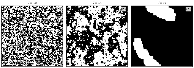
fig_4_17. Reproduces Murphy (2023), Figure 4.17. Download: PDF · SVGThe book says that as the lattice grows there is a critical value \(J_c=\tfrac12\log(1+\sqrt2)\approx0.44\) (4.79), the rapid change in global behaviour being a phase transition. Figure 4.S2 shows it directly.
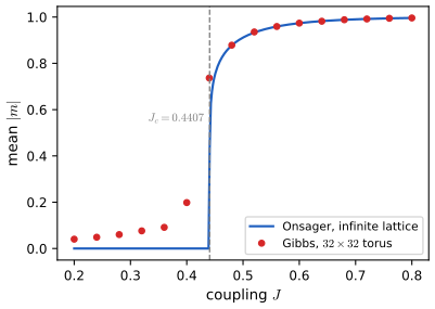
fig_4_S2. Download: PDF · SVG4.3.2.2 Potts models
pp. 169–170, (4.83)–(4.86), Figure 4.18 The Potts model with \(x_i\in\{1,\dots,K\}\) uses \(\psi_{ij}=e^{J}\) if \(x_i=x_j\) and \(1\) otherwise (4.84); with local evidence the energy is \[ -\sum_i\sum_k\alpha_k\ind(x_i=k)-J\sum_{i\sim j}\ind(x_i=x_j) \] (4.86). Its transition for the 2-D lattice is at \(J_c=\log(1+\sqrt K)\) (4.85); for \(K=10\) this is \(1.426\), the value used in Figure 4.18.
Filling the gap 4.9: where the critical couplings \(\tfrac12\log(1+\sqrt2)\) and \(\log(1+\sqrt K)\) come from p. 168, (4.79); p. 169, (4.85)
The book quotes both from the literature. The values are the self-dual points of a duality between low and high temperature; the argument below proves the duality and shows where the numbers come from. That the transition really occurs at the self-dual point is Onsager's (1944) exact solution for the Ising model, and Beffara and Duminil-Copin (2012) for the Potts model, and is not reproved here.
Derivation
High-temperature expansion. For spins \(x,x'=\pm1\), \(e^{Jxx'}=\cosh J\,(1+xx'\tanh J)\) (check \(xx'=\pm1\)). For a lattice with edge set \(E\),
\[ Z(J)=\sum_{\mathbf{x}}\prod_{e=(i,j)\in E}\cosh J\,(1+x_ix_j\tanh J)=(\cosh J)^{|E|}\sum_{A\subseteq E}(\tanh J)^{|A|}\sum_{\mathbf{x}}\prod_{i}x_i^{\deg_A(i)}. \]The sum over spins is \(2^N\) if every vertex has even degree in \(A\) (an even subgraph) and zero otherwise (a spin with odd degree sums to 0). Hence \[ Z(J)=2^N(\cosh J)^{|E|}\sum_{A\text{ even}}(\tanh J)^{|A|} \], which was confirmed by direct enumeration on a \(3\times3\) lattice.
Low-temperature expansion. A spin configuration is determined, up to a global flip, by the set \(\Gamma\) of bonds whose spins disagree, and on a planar lattice such a set corresponds to a collection of closed contours on the dual lattice (even subgraphs of the dual). Each disagreeing bond costs \(e^{-J}/e^{J}=e^{-2J}\) relative to the ground state, so \[ Z(J)=2e^{J|E|}\sum_{\Gamma\text{ even in dual}}(e^{-2J})^{|\Gamma|} \].
Duality. The square lattice is self-dual (its dual is again a square lattice). Define \(J^*\) by \(\tanh J^*=e^{-2J}\). The low-temperature sum for \(J\) is then the high-temperature sum for \(J^*\), so \(Z(J)\) and \(Z(J^*)\) agree up to explicit smooth prefactors, and the free energy is singular at \(J\) iff it is at \(J^*\). If there is a single transition it must sit at the fixed point \(J=J^*\), i.e. \(\tanh J=e^{-2J}\). With \(t=e^{-2J}\), \(\tanh J=(1-t)/(1+t)\), and \((1-t)/(1+t)=t\) gives \(t^2+2t-1=0\), \(t=\sqrt2-1\), so
\[ J_c=-\tfrac12\log(\sqrt2-1)=\tfrac12\log(1+\sqrt2)=0.4407,\qquad\text{equivalently }\sinh(2J_c)=1. \]Potts. With \(v=e^{J}-1\), \(e^{J\ind(x=x')}=1+v\,\ind(x=x')\). Expanding the product over edges, \[ Z=\sum_{A\subseteq E}v^{|A|}\sum_{\mathbf{x}}\prod_{e\in A}\ind(x_i=x_j)=\sum_{A}v^{|A|}K^{c(A)} \], where \(c(A)\) is the number of connected components of \((V,A)\) (each component must be monochromatic): the Fortuin–Kasteleyn random-cluster form. For the planar lattice the dual weight \(v^*\) satisfies \(vv^*=K\), so the self-dual point is \(v=\sqrt K\), \(e^{J}-1=\sqrt K\), \(J_c=\log(1+\sqrt K)\) (4.85). For \(K=2\) this is \(\log(1+\sqrt2)=2\cdot0.4407\), consistent with \(J_P=2J_I\). The transition is continuous for \(K\le4\) and first order for \(K>4\) (Baxter, 1973), so for \(K=10\) a sampler started at random can stay in the disordered phase for a long time just above \(J_c\), which is why Figure 4.18 needs many sweeps.
The Gibbs estimate of the magnetisation of a \(48\times48\) lattice at \(J=0.5\) agrees with Onsager's \(0.9113\) (finite-size effects are tiny this far above \(J_c\)).
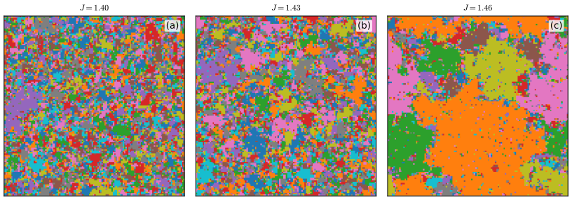
fig_4_18. Reproduces Murphy (2023), Figure 4.18. Download: PDF · SVG4.3.2.3 Potts models for protein structure prediction
p. 170 In direct coupling analysis a Potts model with \(V=21\) states (20 amino acids and a gap) is fitted to a multiple sequence alignment by (pseudo)maximum likelihood; the largest couplings \(J_{ij}\) between positions flag residues in physical contact (a contact map), which feeds structure prediction. This needs the MSA data and large-scale fitting, so it is not reproduced; the fitting method is analysed in Section 4.3.9.
4.3.2.4 Hopfield networks
pp. 170–172, (4.87)–(4.90), Figure 4.19 A Hopfield network is a fully connected Ising model with symmetric weights \(\mathbf{W}=\mathbf{W}^\T\), energy \[ E(\mathbf{x})=-\tfrac12\mathbf{x}^\T\mathbf{W}\mathbf{x} \] (4.87), \(x_i=\pm1\). As an associative memory, a partial pattern is completed by \(\mathbf{x}^*=\arg\min E\) (4.88), found by iterated conditional modes, \[ \mathbf{x}^{t+1}=\mathrm{sgn}(\mathbf{W}\mathbf{x}^t) \] (4.89). The outer-product rule is \[ \mathbf{W}=\big(\tfrac1N\sum_n\mathbf{x}_n\mathbf{x}_n^\T\big)-\mathbf{I} \] (4.90), where \(N\) is the number of stored patterns (not the number of units; below it is written \(P\)).
Filling the gap 4.10: energy descent, symmetric fixed points and capacity of a Hopfield network pp. 171–172, (4.88)–(4.90)
The book does not prove that ICM decreases the energy, and quotes the capacity \(\sim0.14N\).
Derivation
Energy descent. Let \(W_{ii}=0\) and \(W\) symmetric. The terms of \(E\) containing \(x_i\) are \(-x_i f_i\) with \(f_i=\sum_{k}W_{ik}x_k\) (which does not involve \(x_i\)). Setting \(x_i\leftarrow\mathrm{sgn}(f_i)\) minimises \(-x_if_i\) over \(x_i=\pm1\), so each asynchronous update (one site at a time) never increases \(E\); as there are finitely many states, the dynamics reach a fixed point, a local minimum of \(E\). (The zero diagonal in (4.90) is what makes \(f_i\) independent of \(x_i\); \(\mathbf{x}_n\mathbf{x}_n^\T\) has ones on its diagonal, hence the subtraction of \(\mathbf{I}\).) The synchronous rule (4.89) updates all sites at once and need not decrease \(E\); it can end in a 2-cycle. In the code the asynchronous energy is monotone, and the synchronous rule settled in one step on the images below. Because \(E(\mathbf{x})=E(-\mathbf{x})\), the outer-product rule stores the inverse of every pattern too, as the book says.
Crosstalk and capacity. Store \(P\) random \(\pm1\) patterns and present the first. The field on unit \(i\) is \[ f_i=\tfrac1P\sum_n x^n_i(\mathbf{x}^n\cdot\mathbf{x}^1)-x^1_i \]. The \(n=1\) term gives \(\tfrac{N}{P}x_i^1-x_i^1\), and in each term \(n\ge2\) the \(j=i\) part of \(\mathbf{x}^n\cdot\mathbf{x}^1\) gives \(x_i^1\) again, so the signal is \(x^1_i(N-1)/P\); the remaining noise \[ \tfrac1P\sum_{n\ge2}\sum_{j\ne i}x^n_ix^n_jx^1_j \] has mean 0 and variance \((P-1)(N-1)/P^2\). The bit \(i\) is wrong after one step with probability \[ \Phi\big(-\sqrt{(N-1)/(P-1)}\big)\approx\Phi(-\sqrt{N/P}) \]. A simulation with \(N=500\), \(P=60\) gives \(0.0018\), matching the formula's \(0.0018\). So retrieval is almost perfect for \(P\ll N\); but a few wrong bits perturb the next step. Whether the errors avalanche was settled by the replica analysis of Amit, Gutfreund and Sompolinsky (1985), which gives the capacity \(P/N\approx0.138\); that analysis is not reproduced here. Figure 4.S5 shows the transition numerically.
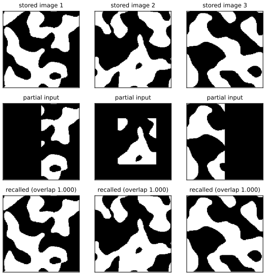
fig_4_19. Reproduces Murphy (2023), Figure 4.19 (with stand-in images). Download: PDF · SVG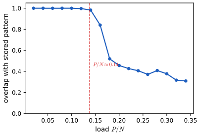
fig_4_S5. Download: PDF · SVG4.3.3 MRFs with latent variables (Boltzmann machines, etc.)
pp. 172–174, (4.91)–(4.92), Figures 4.20–4.22 A fully visible MRF can model correlation only by adding an edge. A Boltzmann machine adds hidden units \(\mathbf{z}\) to an Ising-type model on an arbitrary graph with states \(\{0,1\}\); exact inference is intractable. A restricted Boltzmann machine (RBM, or harmonium) is bipartite: no connections within a layer, so \[ p(\mathbf{z}\given\mathbf{x})=\prod_kp(z_k\given\mathbf{x}) \], in contrast with a directed two-layer model, where explaining away entangles the hidden units. Stacking layers gives a deep Boltzmann machine (4.91), \[ p(\mathbf{x},\mathbf{z}_1,\mathbf{z}_2)\propto\exp(\mathbf{x}^\T\mathbf{W}_1\mathbf{z}_1+\mathbf{z}_1^\T\mathbf{W}_2\mathbf{z}_2) \], and an RBM on top of a directed decoder gives a deep belief network (4.92), which is not a belief net (the book proposes calling it a deep Boltzmann network). Table 4.4 lists variants by visible and hidden type.
4.3.3.2 Restricted Boltzmann machines (RBMs)
RBMs in more detail (supplement 4.3)
Supp. pp. 46–48, (4.8)–(4.22) The binary RBM has joint \(p(\mathbf{x},\mathbf{z})=Z^{-1}\exp(-E)\) with \[ E(\mathbf{x},\mathbf{z})=-(\mathbf{x}^\T\mathbf{W}\mathbf{z}+\mathbf{x}^\T\mathbf{b}+\mathbf{z}^\T\mathbf{c}) \] (supplement 4.8)–(4.10), a \(D\times K\) weight matrix, visible bias \(\mathbf{b}\) and hidden bias \(\mathbf{c}\); the posterior is \[ p(\mathbf{z}\given\mathbf{x})=\prod_k\mathrm{Ber}(z_k\given\sigma(\mathbf{w}_{:,k}^\T\mathbf{x}+c_k)) \] (supplement 4.12); \[ \mathbb{E}[\mathbf{z}\given\mathbf{x}]=\sigma(\mathbf{W}^\T\mathbf{x}) \] and \[ \mathbb{E}[\mathbf{x}\given\mathbf{z}]=\sigma(\mathbf{W}\mathbf{z}) \] (with biases) (supplement 4.14)–(4.15) are the recognition and generative weights. A hidden unit \(k\) adds the term \(\mathbf{w}_k^\T\mathbf{x}\) to the energy when on, a "soft constraint"; turning on a subset of units multiplies the corresponding experts, so the model is a product of experts and a mixture of \(2^K\) components (a distributed representation), whereas a standard mixture model has \(K\) components (localist). The "doping" example of the supplement is the intersection of "sports" and "drugs" rather than their union.
Filling the gap 4.11: the RBM conditionals, free energy, mixture view and learning gradient Supp. pp. 46–47; main pp. 172–173
The supplement states the conditionals "by symmetry" and "one can show". Here are the derivations, and the contrast with a directed model.
Derivation
Conditionals. The energy is linear in each \(z_k\): \[ -E=\sum_kz_k(c_k+\mathbf{w}_{:,k}^\T\mathbf{x})+\mathbf{b}^\T\mathbf{x} \]. Hence \[ p(\mathbf{z}\given\mathbf{x})\propto\prod_k\exp\{z_k(c_k+\mathbf{w}_{:,k}^\T\mathbf{x})\} \], a product over \(k\), so the \(z_k\) are conditionally independent and \[ p(z_k=1\given\mathbf{x})=e^{a_k}/(1+e^{a_k})=\sigma(a_k) \] with \(a_k=c_k+\mathbf{w}_{:,k}^\T\mathbf{x}\) (supplement 4.12). The same argument in \(x_d\) gives (4.13). Both were confirmed by brute-force enumeration for a small RBM.
Free energy. Summing out each \(z_k\in\{0,1\}\) separately,
\[ \tilde p(\mathbf{x})=\sum_{\mathbf{z}}e^{-E}=e^{\mathbf{b}^\T\mathbf{x}}\prod_k\big(1+e^{c_k+\mathbf{w}_{:,k}^\T\mathbf{x}}\big)=e^{-F(\mathbf{x})},\quad F(\mathbf{x})=-\mathbf{b}^\T\mathbf{x}-\sum_k\mathrm{softplus}(c_k+\mathbf{w}_{:,k}^\T\mathbf{x}). \]So \(p(\mathbf{x})=e^{-F(\mathbf{x})}/Z\) and \(Z=\sum_{\mathbf{x}}e^{-F(\mathbf{x})}\), at cost \(O(2^DDK)\); summing out \(\mathbf{x}\) first gives the symmetric form with cost \(O(2^KDK)\). This is the reduction of the naive \(2^{D+K}\) to \(\min\{2^D,2^K\}\) times a polynomial factor claimed in the supplement (its printed exponents are lost in the text). The three ways of computing \(\log Z\) agree numerically. Mixture view. \[ p(\mathbf{x})=\sum_{\mathbf{z}}p(\mathbf{z})p(\mathbf{x}\given\mathbf{z}) \] with \[ p(\mathbf{x}\given\mathbf{z})\propto\exp\big((\mathbf{b}+\mathbf{W}\mathbf{z})^\T\mathbf{x}\big)=\prod_{k:z_k=1}e^{\mathbf{w}_{:,k}^\T\mathbf{x}}\cdot e^{\mathbf{b}^\T\mathbf{x}} \]: a product of the experts that are on.
Learning. Apply (4.135) of the book: with \(\theta=\mathbf{W}\) and features \(x_dz_k\), \[ \partial\ell/\partial W_{dk}=\mathbb{E}_{\mathrm{data}}[x_d\,\mathbb{E}(z_k\given\mathbf{x})]-\mathbb{E}_{p(\mathbf{x},\mathbf{z})}[x_dz_k] \]: clamped phase minus unclamped phase. The first term is cheap because of the conditional above; the second is an intractable expectation, and contrastive divergence (CD-1) replaces it by a single Gibbs step started at the data (Chapter 24 of the book). A finite-difference check on a small RBM reproduces the exact gradient to \(10^{-7}\). In Figure 4.21 CD-1 on binarised MNIST (100 hidden units, 5 epochs) makes the reconstruction of unseen digits steadily better.
Contrast with a directed layer. In a two-layer sigmoid belief net the hidden units are independent in the prior but, given a visible child, the posterior over them does not factorise: for two hidden units with Bernoulli(1/2) priors and an observed unit \(x=1\), \[ p(z_1,z_2\given x=1)\propto\sigma(2z_1+2z_2-2.5) \] differs from the product of its marginals by up to 0.03 in a numerical example, whereas for an RBM the posterior is exactly a product.
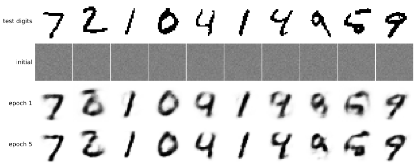
fig_4_21 (about 20 s). Reproduces Murphy (2023), Figure 4.21 (the book shows images generated by its own run). Download: PDF · SVGFilling the gap 4.12: categorical and Gaussian RBMs (supplement) Supp. pp. 47–48, (4.16)–(4.22)
The supplement lists the full conditionals of the categorical and Gaussian RBMs without derivation.
Derivation
Categorical visible units. With a one-of-\(C\) coding \(x_d^c\in\{0,1\}\), \(\sum_cx_d^c=1\), the energy (4.16) is linear in each \(\mathbf{x}_d\) given \(\mathbf{z}\): \[ -E=\sum_d\sum_cx_d^c(b_d^c+\sum_kz_kw_{dk}^c)+\sum_kz_kc_k \]. Thus \[ p(x_d=c\given\mathbf{z})\propto\exp(b_d^c+\sum_kz_kw^c_{dk}) \], the softmax (4.17); and \[ p(z_k=1\given\mathbf{x})=\sigma(c_k+\sum_{d,c}x_d^cw_{dk}^c) \] (4.18). Gaussian visible units. With the quadratic term entered with its correct positive sign (see the list of errors at the end), the \(x\)-dependent part of the Gaussian-RBM energy (4.19) is \(-x_d\sum_kw_{dk}z_k+\tfrac12(x_d-b_d)^2\); completing the square, \[ \tfrac12(x_d-b_d-\sum_kw_{dk}z_k)^2+\mathrm{const} \], so \[ p(x_d\given\mathbf{z})=\N(b_d+\sum_kw_{dk}z_k,1) \] (4.21), checked by quadrature. In information form \(\bm\Lambda=\mathbf{I}\) and \(\bm\eta=\sum_kz_k\mathbf{w}_{:,k}\), so the mean is the weighted sum of the prototypes of the active hidden units. The hidden conditional (4.22) is again a sigmoid (note that (4.19) writes the hidden bias as \(a_k\) and (4.22) as \(c_k\): one symbol is meant). With Gaussian hidden units too, the joint is a Gaussian and the model is an undirected version of factor analysis, mathematically equivalent to the directed one (Marks and Movellan, 2001), as the supplement says.
4.3.3.3 Deep Boltzmann machines and 4.3.3.4 deep belief networks
Described above; DBNs trained greedily played an important role in the history of deep learning but have been replaced by supervised networks with ReLU units and Adam, and by deep directed generative models such as VAEs (Section 21.2). The sampler for a DBM is Gibbs sampling over layers, because within a layer the units are conditionally independent given its neighbours.
4.3.4 Maximum entropy models
pp. 174–176, (4.93)–(4.100) The exponential family \[ p(\mathbf{x}\given\theta)=Z(\theta)^{-1}\exp(\theta^\T\bm\phi(\mathbf{x})) \] (4.93) is the maximum entropy distribution with given feature expectations (Section 2.4.7). If the features decompose over the cliques of a graph this is a maxent model or log-linear model \[ p(\mathbf{x})=Z^{-1}\exp(\sum_c\theta_c^\T\bm\phi(x_c)) \] (4.94)–(4.95); Gaussian graphical models have \(\bm\phi([x_i,x_j])=[x_i,x_j,x_ix_j]\) (4.96) and so do Ising models (4.97). The partition function costs \(O(D^3)\) for a Gaussian and \(O(2^D)\) in general. Feature induction (Della Pietra et al., 1997; 4.98–4.100) greedily adds features; in the book's English-spelling example the first feature \(\phi_1=\sum_i\ind(x_i\in\{a,\dots,z\})\) has fitted weight \(\hat\theta_1=1.944\), so a word with a lowercase letter in a position is \(e^{1.944}\approx7\) times more likely than one without. (The samples shown use annealed Gibbs sampling on a large corpus-trained model and are not reproduced.)
Filling the gap 4.13: why the exponential family is the maximum entropy distribution p. 174, (4.93)
The book refers to Section 2.4.7 (the exponential family has maximum entropy subject to matching the empirical feature expectations). A short proof, for discrete \(\mathbf{x}\) (densities are the same with integrals and differential entropy).
Proof
Let \[ p_\theta(\mathbf{x})=\exp(\theta^\T\bm\phi(\mathbf{x}))/Z(\theta) \] have \(\mathbb{E}_{p_\theta}[\bm\phi]=\mathbf{m}\), and let \(q\) be any distribution with \(\mathbb{E}_q[\bm\phi]=\mathbf{m}\). Then \[ \mathbb{E}_q[\log p_\theta]=\theta^\T\mathbf{m}-\log Z(\theta)=\mathbb{E}_{p_\theta}[\log p_\theta] \] because \(\log p_\theta\) is affine in \(\bm\phi\) and the two expectations of \(\bm\phi\) agree. Therefore \[ H(q)=-\mathbb{E}_q[\log q]=-\mathbb{E}_q[\log p_\theta]-\mathrm{KL}(q\,\|\,p_\theta)=H(p_\theta)-\mathrm{KL}(q\,\|\,p_\theta)\le H(p_\theta) \], with equality iff \(q=p_\theta\) (KL is non-negative and zero only for equality). So \(p_\theta\) is the unique maximiser of the entropy among distributions with the moments \(\mathbf{m}\). That a \(\theta\) with these moments exists when \(\mathbf{m}\) is in the interior of the set of achievable moments follows from the strict concavity of the likelihood (Result 4.10); the companion treatment of the same fact is in Filling the gap 10.12 of the first volume's course. A numerical experiment on six outcomes with two constraints: direct constrained entropy maximisation and the exponential family with matched moments agree to \(10^{-9}\). ∎
4.3.5 Gaussian MRFs
pp. 177–179, (4.101)–(4.114) A Gaussian MRF (Gaussian graphical model, GGM) is the pairwise MRF \[ p(\mathbf{x})=Z^{-1}\prod_{i\sim j}\psi_{ij}\prod_i\psi_i \] with \(\psi_{ij}=\exp(-\tfrac12x_i\Lambda_{ij}x_j)\), \[ \psi_i=\exp(-\tfrac12\Lambda_{ii}x_i^2+\eta_ix_i) \] (4.101)–(4.103), i.e. \[ p(\mathbf{x})\propto\exp(\bm\eta^\T\mathbf{x}-\tfrac12\mathbf{x}^\T\bm\Lambda\mathbf{x}) \] (4.105), the information form with \(\bm\Lambda=\bm\Sigma^{-1}\), \(\bm\eta=\bm\Lambda\bm\mu\). Zeros of \(\bm\Lambda\) ("structural zeros") are missing edges, which is what \(\ell_1\)-regularised graph estimation (the graphical lasso) exploits.
Result 4.8 (the Gaussian MRF) pp. 177–178, (4.101)–(4.107)
(a) \[ Z(\theta)=\int\exp(\bm\eta^\T\mathbf{x}-\tfrac12\mathbf{x}^\T\bm\Lambda\mathbf{x})\,d\mathbf{x}=(2\pi)^{D/2}|\bm\Lambda|^{-1/2}\exp\big(\tfrac12\bm\eta^\T\bm\Lambda^{-1}\bm\eta\big) \] for positive definite \(\bm\Lambda\). (b) \(x_i\indep x_j\given\mathbf{x}_{-ij}\) iff \(\Lambda_{ij}=0\), and the partial correlation is \[ \rho_{ij\cdot\mathrm{rest}}=-\Lambda_{ij}/\sqrt{\Lambda_{ii}\Lambda_{jj}} \]. (c) For the stationary AR(1) process \(x_t=\rho x_{t-1}+\tau\epsilon_t\), \(x_1\sim\N(0,\tau^2/(1-\rho^2))\), the precision matrix is the tridiagonal (4.106) and the covariance is
\[ \Sigma_{ij}=\frac{\tau^2}{1-\rho^2}\rho^{|i-j|}, \tag{replaces 4.107} \]dense although the precision matrix is sparse.
Proof
(a) Complete the square: \[ \bm\eta^\T\mathbf{x}-\tfrac12\mathbf{x}^\T\bm\Lambda\mathbf{x}=-\tfrac12(\mathbf{x}-\bm\mu)^\T\bm\Lambda(\mathbf{x}-\bm\mu)+\tfrac12\bm\mu^\T\bm\Lambda\bm\mu \] with \(\bm\mu=\bm\Lambda^{-1}\bm\eta\), and \[ \bm\mu^\T\bm\Lambda\bm\mu=\bm\eta^\T\bm\Lambda^{-1}\bm\eta \]; the Gaussian integral gives \((2\pi)^{D/2}|\bm\Lambda|^{-1/2}\). (b) The exponent contains \(x_i\) and \(x_j\) together only through \(-\Lambda_{ij}x_ix_j\). If \(\Lambda_{ij}=0\) the density given the rest factorises as a function of \(x_i\) times a function of \(x_j\) (factorisation criterion), so they are conditionally independent. Conversely the conditional of \((x_i,x_j)\) given the rest is Gaussian with precision the \(2\times2\) block \[ \begin{pmatrix}\Lambda_{ii}&\Lambda_{ij}\\\Lambda_{ij}&\Lambda_{jj}\end{pmatrix} \] (read off the quadratic form), whose covariance has off-diagonal entry \[ -\Lambda_{ij}/(\Lambda_{ii}\Lambda_{jj}-\Lambda_{ij}^2) \]; a Gaussian pair is independent iff this is zero, and the correlation is \(-\Lambda_{ij}/\sqrt{\Lambda_{ii}\Lambda_{jj}}\). The residual-correlation form was checked numerically. See also Theorems 18.J and 18.K. (c) The DAG form \(x_1\sim\N(0,s_1^2)\), \(x_t\given x_{t-1}\sim\N(\rho x_{t-1},\tau^2)\) with \(s_1^2=\tau^2/(1-\rho^2)\) has, by Result 4.2, \[ \bm\Lambda=\sum_i\sigma_i^{-2}(\mathbf{e}_i-\mathbf{w}_i)(\mathbf{e}_i-\mathbf{w}_i)^\T \]: node 1 contributes \(s_1^{-2}=(1-\rho^2)/\tau^2\) at \((1,1)\); node \(t\ge2\) contributes \(\tau^{-2}\) at \((t,t)\), \(\rho^2\tau^{-2}\) at \((t-1,t-1)\) and \(-\rho\tau^{-2}\) at \((t,t-1)\) and \((t-1,t)\). The \((1,1)\) entry is \(\tau^{-2}(1-\rho^2+\rho^2)=\tau^{-2}\), the interior ones \(\tau^{-2}(1+\rho^2)\), the last one \(\tau^{-2}\): this is (4.106). The covariance of a stationary AR(1) is \(\mathrm{Cov}(x_i,x_j)=\rho^{|i-j|}s_1^2\) (induction: \(\mathrm{Var}(x_t)=\rho^2s_1^2+\tau^2=s_1^2\), \[ \mathrm{Cov}(x_t,x_{t+k})=\rho^k\mathrm{Var}(x_t) \]), and \(\bm\Lambda\bm\Sigma=\mathbf{I}\) was verified for \(T=7\). ∎
An error in (4.104) and (4.107)
(1) The book gives \(Z(\theta)=(2\pi)^{D/2}|\bm\Lambda|^{-1/2}\) (4.104) for the model with linear terms \(\eta_ix_i\); this is the normaliser only when \(\bm\eta=0\): in general there is the factor \[ \exp(\tfrac12\bm\eta^\T\bm\Lambda^{-1}\bm\eta) \] of Result 4.8(a) (checked by numerical integration in two dimensions). (2) The matrix printed in (4.107) as \(\bm\Lambda^{-1}\) has diagonal \(\tau^2\rho\) and entries \(\tau^2\rho^{|i-j|+1}\); that cannot be the inverse of (4.106): its diagonal \(\tau^2\rho\) is smaller than the variance \(\tau^2/(1-\rho^2)\ge\tau^2\) of the stationary process. The correct covariance is \(\tau^2\rho^{|i-j|}/(1-\rho^2)\); with \(\rho=0.6\), \(\tau=1\) its first row is \(1.5625,0.9375,0.5625,\dots\) and the product of (4.106) with the printed (4.107) differs from the identity by up to 0.62. The statement the book draws from it is correct: the covariance is dense although the precision is sparse.
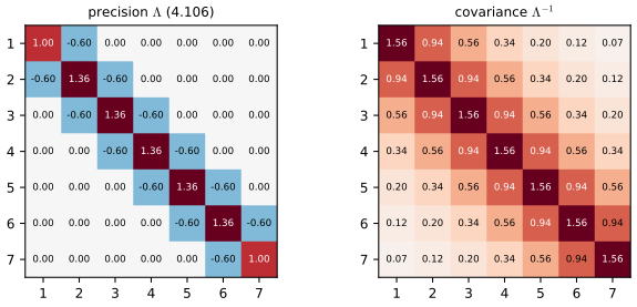
fig_4_S1. Download: PDF · SVG4.3.5.2 Nonlinear Gaussian MRFs
A nonlinear Gaussian MRF has \(p(\mathbf{x})=Z^{-1}\prod_c\psi_c(x_c)\), \(\psi_c=\exp(-E_c)\), \[ E_c=\tfrac12(f_c(x_c)-d_c)^\T\bm\Sigma_c^{-1}(f_c(x_c)-d_c) \] (4.108)–(4.110). For linear \(f_c(x)=\mathbf{J}_cx+\mathbf{b}_c\) (4.111) the energy is a Gaussian factor with \[ \bm\Lambda_c=\mathbf{J}_c^\T\bm\Sigma_c^{-1}\mathbf{J}_c \] and \[ \bm\eta_c=\mathbf{J}_c^\T\bm\Sigma_c^{-1}(d_c-\mathbf{b}_c) \] (4.112)–(4.113); for nonlinear \(f_c\) one linearises about a current estimate \(x_c^0\) (4.114) and iterates.
Filling the gap 4.14: iterating the linearisation is the Gauss–Newton method p. 178, (4.112)–(4.114)
The book says "this process can be iterated". What it computes is a known optimiser.
Derivation
Expand \(E_c\) for linear \(f_c\): \[ \tfrac12(\mathbf{J}x+\mathbf{b}-d)^\T\bm\Sigma^{-1}(\mathbf{J}x+\mathbf{b}-d)=\tfrac12x^\T\mathbf{J}^\T\bm\Sigma^{-1}\mathbf{J}x+x^\T\mathbf{J}^\T\bm\Sigma^{-1}(\mathbf{b}-d)+k \], which is (4.112) with \(\bm\Lambda_c\), \(-\bm\eta_c\), \(k_c\) as stated (expand and compare). For nonlinear \(f_c\), \(\mathbf{b}_c=f_c(x^0)-\mathbf{J}_cx^0\) (4.114). The Gaussian with \(\bm\Lambda=\sum_c\bm\Lambda_c\), \(\bm\eta=\sum_c\bm\eta_c\) has mode \[ \bm\Lambda^{-1}\bm\eta=x^0+\bm\Lambda^{-1}\sum_c\mathbf{J}_c^\T\bm\Sigma_c^{-1}(d_c-f_c(x^0))=x^0-\bm\Lambda^{-1}\nabla E(x^0) \], because \[ \nabla E=\sum_c\mathbf{J}_c^\T\bm\Sigma_c^{-1}(f_c-d_c) \]. That is the Gauss–Newton step for minimising the nonlinear least-squares energy \(E\): it uses \[ \bm\Lambda=\sum_c\mathbf{J}_c^\T\bm\Sigma_c^{-1}\mathbf{J}_c \] in place of the Hessian, dropping the terms with second derivatives of \(f_c\). So the iterated "temporary Gaussian factor" gives the MAP estimate of the nonlinear model, and \(\bm\Lambda\) at the last iterate is a Gaussian (Laplace-type) approximation of the posterior precision; the sparsity of \(\bm\Lambda\) is that of the factor graph.
4.3.5.3 INLA approximation
p. 179 For latent Gaussian models \[ p(\mathbf{y},\mathbf{x}\given\theta)=p(\mathbf{x}\given\theta)\prod_ip(y_i\given x_i,\theta) \] with a GMRF prior on \(\mathbf{x}\), the integrated nested Laplace approximation (INLA; Rue et al., 2009) approximates \(p(\theta\given\mathbf{y})\) using \[ p(\mathbf{y}\given\theta)=p(\mathbf{y}\given\mathbf{x}^*,\theta)p(\mathbf{x}^*\given\theta)/p(\mathbf{x}^*\given\mathbf{y},\theta) \] at the mode \(\mathbf{x}^*\) of a Gaussian approximation of \(p(\mathbf{x}\given\mathbf{y},\theta)\).
Filling the gap 4.15: the Laplace step of INLA, exactly p. 179
The identity and the iteration are stated without derivation.
Derivation
The identity. By the product rule \[ p(\mathbf{y},\mathbf{x}\given\theta)=p(\mathbf{y}\given\theta)p(\mathbf{x}\given\mathbf{y},\theta) \] for every \(\mathbf{x}\); solve for \(p(\mathbf{y}\given\theta)\). It becomes an approximation when the denominator \(p(\mathbf{x}^*\given\mathbf{y},\theta)\) is replaced by its Gaussian approximation \[ \N(\mathbf{x}\given\mathbf{x}^*,\bm\Lambda_*^{-1}) \] evaluated at its mean, which equals \((2\pi)^{-D/2}|\bm\Lambda_*|^{1/2}\):
\[ \log p(\mathbf{y}\given\theta)\approx\log p(\mathbf{y}\given\mathbf{x}^*,\theta)+\log p(\mathbf{x}^*\given\theta)-\tfrac12\log|\bm\Lambda_*|+\tfrac D2\log2\pi. \]This is exact when \(\mathbf{y}\given\mathbf{x}\) is Gaussian (then \(p(\mathbf{x}\given\mathbf{y})\) is exactly Gaussian); a check with \(\mathbf{x}\sim\N(0,\bm\Sigma)\), \[ \mathbf{y}\given\mathbf{x}\sim\N(\mathbf{x},s^2\mathbf{I}) \] reproduces \[ \log\N(\mathbf{y}\given0,\bm\Sigma+s^2\mathbf{I}) \] to rounding error.
The iteration. Let \[ L(\mathbf{x})=\log p(\mathbf{x}\given\theta)+f(\mathbf{x}) \] with \(f=\log p(\mathbf{y}\given\mathbf{x},\theta)\), gradient \(\mathbf{g}\) and diagonal Hessian \(\mathbf{H}\) (the likelihood factorises over nodes). The gradient of \(L\) is \[ -\bm\Sigma^{-1}(\mathbf{x}-\bm\mu)+\mathbf{g}(\mathbf{x}) \] and its Hessian \(-\bm\Sigma^{-1}+\mathbf{H}(\mathbf{x})\). A Newton step from \(\mathbf{x}^0\) with \(\mathbf{A}=\bm\Sigma^{-1}-\mathbf{H}_0\):
\[ \mathbf{x}^1=\mathbf{x}^0+\mathbf{A}^{-1}\big(-\bm\Sigma^{-1}(\mathbf{x}^0-\bm\mu)+\mathbf{g}_0\big)=\mathbf{A}^{-1}\big(\bm\Sigma^{-1}\bm\mu+\mathbf{g}_0-\mathbf{H}_0\mathbf{x}^0\big)=\bm\Lambda_0^{-1}\bm\eta_0, \]using \[ \mathbf{A}\mathbf{x}^0-\bm\Sigma^{-1}\mathbf{x}^0=-\mathbf{H}_0\mathbf{x}^0 \]: so the book's "precision \(\bm\Sigma^{-1}-\mathbf{H}_0\) and precision-weighted mean \[ \bm\Sigma^{-1}\bm\mu+\mathbf{g}_0-\mathbf{H}_0\mathbf{x}^0 \]" is exactly Newton's method on the log joint. Since \(\mathbf{H}_0\) is diagonal, \(\mathbf{A}\) has the sparsity pattern of \(\bm\Sigma^{-1}\) (the GMRF precision), so each step is one sparse linear solve and the sparse Cholesky symbolic pattern is reused. The marginals \[ p(x_i\given\mathbf{y})=\int p(x_i\given\theta,\mathbf{y})p(\theta\given\mathbf{y})d\theta \] are finally obtained by numerical integration over a few values of \(\theta\), feasible only when \(\theta\) is low-dimensional.
4.3.6 Conditional independence properties
4.3.6.1 Basic results
pp. 179–180, (4.115)–(4.116), Figures 4.23–4.24 In a UPGM, \(X_A\indep X_B\given X_C\) iff \(C\) separates \(A\) from \(B\): after deleting the nodes of \(C\) no path joins \(A\) to \(B\) (the global Markov property). The Markov blanket of \(t\), the smallest set with \[ t\indep V\setminus\mathrm{cl}(t)\given\mathrm{mb}(t) \] (4.115), is its set of neighbours (the local property), and \[ s\indep t\given V\setminus\{s,t\}\iff G_{st}=0 \] (4.116) is the pairwise property.
Result 4.9 (the undirected Markov properties) p. 180, Figure 4.24
For every distribution, global \(\Rightarrow\) local \(\Rightarrow\) pairwise. For strictly positive distributions all three are equivalent (and equivalent to the Gibbs factorisation of Result 4.7). Without positivity pairwise does not imply global.
Proof
Global \(\Rightarrow\) local: \(\mathrm{mb}(t)\) (the neighbours) separates \(t\) from the rest. Local \(\Rightarrow\) pairwise: if \(s,t\) are non-adjacent, \(s\) lies outside \(\mathrm{cl}(t)\), so \(t\indep s\given\mathrm{mb}(t)\), and weak union (adding \(V\setminus(\{s,t\}\cup\mathrm{mb}(t))\) to the conditioning set) gives \(t\indep s\given V\setminus\{s,t\}\). For positive \(p\), pairwise implies the Gibbs factorisation (the Möbius-inversion half of Result 4.7), and factorisation over cliques implies the global property (Result 8.12). The counterexample without positivity uses deterministic dependencies, e.g. two copies of one variable (Filling the gap 18.4). ∎
For Figure 4.23(b) the book lists \(X_1\indep X_7\given\text{rest}\) (pairwise), \(X_1\indep\text{rest}\given X_2,X_3\) (local) and \[ \{X_1,X_2\}\indep\{X_6,X_7\}\given\{X_3,X_4,X_5\} \] (global), and \(\mathrm{mb}(X_5)=\{X_2,X_3,X_4,X_6,X_7\}\); the code confirms all of them on the graph read off the figure.
4.3.6.2 An undirected alternative to d-separation
pp. 181, Figures 4.23, 4.25 Dropping the arrows of a DAG is wrong (a v-structure \(A\to B\leftarrow C\) would become the chain \(A-B-C\), which asserts \(A\indep C\given B\)). Moralisation marries the parents of each node first. It loses independences (\(X_4\indep X_5\given X_2\) holds in the DAG but the moral edge \(4-5\) hides it), unless one first forms the ancestral graph: delete every node that is neither in \(U=A\cup B\cup C\) nor an ancestor of \(U\), then moralise and test separation. This is exactly part (b) of Result 4.3, and the moralisation correctness and minimality are Result 8.15.
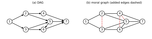
moralize. Code: fig_4_23. Reproduces Murphy (2023), Figure 4.23. Download: PDF · SVG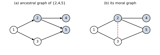
fig_4_25. Reproduces Murphy (2023), Figure 4.25. Download: PDF · SVG4.3.7 Generation (sampling)
pp. 181–182 Without an ordering there is no ancestral sampling, and even unconditional sampling needs MCMC (Chapter 12); the probability of a configuration is not available without \(Z\). For low treewidth with discrete or Gaussian potentials the junction tree gives exact samples by dynamic programming (Supplement Section 9.2.3). The checkerboard Gibbs sampler of Filling the gap 4.8 is the practical method on lattices.
4.3.8 Inference
pp. 182–183, (4.117), Figures 4.26–4.27 Let \(z_i\in\{\pm1\}\) be the pixels of a clean image and \(x_i\) noisy observations with \[ p(\mathbf{x},\mathbf{z})=\big[Z^{-1}\prod_{i\sim j}\psi_{ij}(z_i,z_j)\big]\prod_ip(x_i\given z_i) \], \(p(x_i\given z_i)=\N(x_i\given z_i,\sigma^2)\) (4.117): an undirected prior and a directed likelihood, a hybrid called a chain graph. The task is the posterior marginals or the MAP image; exact inference is intractable on a large grid (Section 9.5.4), and the book uses mean field (Section 10.3.2).
Filling the gap 4.16: the mean-field update for the Ising denoiser p. 183, (4.117), Figure 4.27
The book applies mean field without writing the update. For the Ising prior \(\psi_{ij}=e^{Jz_iz_j}\) and Gaussian noise it is \[ \mu_i\leftarrow\tanh\big(J\sum_{j\sim i}\mu_j+x_i/\sigma^2\big) \].
Derivation
Posterior. Because \(z_i^2=1\), \[ \log\N(x_i\given z_i,\sigma^2)=\text{const}+z_ix_i/\sigma^2 \], so the posterior is \[ p(\mathbf{z}\given\mathbf{x})\propto\exp\big(J\sum_{i\sim j}z_iz_j+\sum_iz_ix_i/\sigma^2\big) \], an Ising model with a site-dependent field \(x_i/\sigma^2\). Mean field. Approximate it by \(q(\mathbf{z})=\prod_iq_i(z_i)\) with means \(\mu_i=\mathbb{E}_q[z_i]\). Coordinate ascent on the evidence lower bound sets \[ \log q_i(z_i)=\mathbb{E}_{q_{-i}}[\log\tilde p(\mathbf{z})]+\text{const} \], and \(\mathbb{E}_{q_{-i}}\) of the terms containing \(z_i\) is \[ z_i\big(J\sum_{j\sim i}\mu_j+x_i/\sigma^2\big)=:z_ia_i \]. So \(q_i(z_i=+1)=e^{a_i}/(e^{a_i}+e^{-a_i})\) and \(\mu_i=\tanh(a_i)\). Order of updates. \(a_i\) depends only on the neighbours of \(i\), which on a bipartite (even) lattice are all of the other checkerboard colour, so one colour can be updated in parallel and this is still exact coordinate ascent. Each update does not decrease the lower bound (it maximises it over \(q_i\)), which was observed numerically; the final bound is below \(\log Z\) (34.42 against 34.43 on a \(4\times4\) torus). Quality. Mean field is exact only in the limit of weak coupling: on that \(4\times4\) problem the means differ from the exact posterior means by 0.016 on average, and Gibbs sampling (40,000 sweeps) reproduces the exact means to 0.02. In Figure 4.27 the fraction of pixels with the right sign rises from 68.6% (thresholding the noisy image) to 96.6% after 15 sweeps. With \(J=0\) the update reduces to \(\mu_i=\tanh(x_i/\sigma^2)\) per pixel, which does no better than thresholding; with a very strong prior (\(J=2\)) thin structures are eroded.
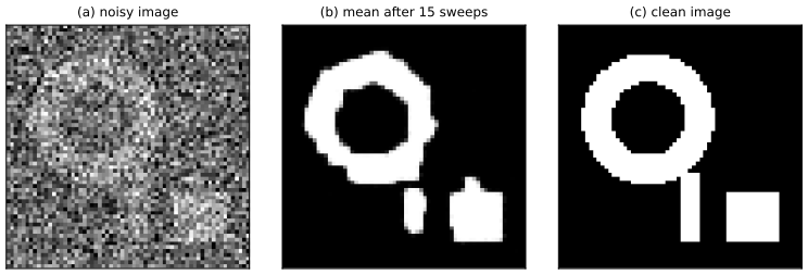
fig_4_27. Reproduces Murphy (2023), Figure 4.27. Download: PDF · SVG4.3.9 Learning
pp. 182–186, (4.118)–(4.135), Figure 4.28 Maximum likelihood for an MRF is expensive even with complete data because of \(Z(\theta)\), and the posterior over \(\theta\) is "doubly intractable" (it needs both \(Z(\theta)\) and \(p(D)\)); so point estimates are used.
4.3.9.1 Learning from complete data and 4.3.9.2 computational issues
Result 4.10 (maximum likelihood for log-linear MRFs is moment matching) pp. 183–184, (4.118)–(4.126)
Let \[ p(\mathbf{x}\given\theta)=Z(\theta)^{-1}\exp(\theta^\T\bm\phi(\mathbf{x})) \] (4.118) and \[ \ell(\theta)=\tfrac1N\sum_n\log p(\mathbf{x}_n\given\theta) \]. Then \(\nabla\log Z=\mathbb{E}_\theta[\bm\phi]\) (4.121), \[ \nabla^2\log Z=\mathrm{Cov}_\theta(\bm\phi)\succeq0 \], so
\[ \nabla\ell(\theta)=\mathbb{E}_{p_D}[\bm\phi]-\mathbb{E}_{p_\theta}[\bm\phi]\tag{4.122} \]and \(\ell\) is concave; \(\hat\theta\) is a maximiser iff \[ \mathbb{E}_{p_D}[\bm\phi]=\mathbb{E}_{p_{\hat\theta}}[\bm\phi] \] (4.123). It is unique when the features are affinely independent. Every gradient evaluation needs an expectation under the model: \[ \nabla\log Z=\mathbb{E}_{p}[\nabla\log\tilde p] \] (4.124)–(4.126).
Proof
Differentiate under the sum (finite) or integral: \[ \partial_\theta\log Z=Z^{-1}\sum_{\mathbf{x}}\bm\phi(\mathbf{x})e^{\theta^\T\bm\phi}=\mathbb{E}_\theta[\bm\phi] \]. A second derivative gives \[ Z^{-1}\sum\bm\phi\bm\phi^\T e^{\theta^\T\bm\phi}-\mathbb{E}[\bm\phi]\mathbb{E}[\bm\phi]^\T=\mathrm{Cov}_\theta(\bm\phi) \], positive semidefinite, and positive definite iff no non-zero \(a\) makes \(a^\T\bm\phi\) constant. Since \[ \ell(\theta)=\theta^\T\mathbb{E}_{p_D}[\bm\phi]-\log Z(\theta) \] with linear first term, \(\ell\) is concave with gradient (4.122) and Hessian \(-\mathrm{Cov}_\theta(\bm\phi)\). The gradient vanishes at (4.123), a global maximum by concavity. The log-derivative trick (4.124)–(4.126) is the identity \(\nabla\tilde p=\tilde p\,\nabla\log\tilde p\) applied inside \(Z^{-1}\nabla\sum\tilde p\), valid for any \(\tilde p\) (not only log-linear). Numerically, on a 5-node Ising ring with 10 features, the finite-difference gradient of \(\log Z\) equals the feature expectation to \(10^{-7}\), the covariance is positive semidefinite, and Newton's method (Hessian \(-\mathrm{Cov}\)) reaches the moment-matching solution to \(10^{-9}\). ∎
The positive phase (data expectation) is the clamped phase, the negative phase the unclamped phase. A first-volume account of "the MLE of a maxent model matches the features" is Filling the gap 10.12.
Filling the gap 4.17: iterative proportional fitting p. 184, footnote 9
For tabular clique potentials the book says moment matching can be solved by IPF, which converges in one iteration on decomposable graphs.
Derivation
The model is \(p\propto\prod_c\psi_c(x_c)\), and the moment-matching conditions say that the marginal of \(p\) on each clique equals the empirical clique marginal \(\hat p_c\). IPF starts from the uniform table and, cycling over cliques, multiplies \(p\) by \(\hat p_c(x_c)/p_c(x_c)\), where \(p_c\) is the current clique marginal. Each step keeps \(p\) in the model (it only rescales the \(\psi_c\)), makes clique \(c\) match its target, and is the exact maximisation of the likelihood over \(\psi_c\) with the others fixed, i.e. coordinate ascent on a concave objective; its convergence is Theorem 19.B of All of Statistics. Chain A–B–C with cliques \(\{A,B\}\), \(\{B,C\}\). From the uniform table, fitting \(\{A,B\}\) gives \(p^1=\hat p(a,b)/|C|\), whose \(\{B,C\}\) marginal is \(\hat p(b)/|C|\). Fitting \(\{B,C\}\) multiplies by \(\hat p(b,c)|C|/\hat p(b)\): \[ p^2(a,b,c)=\hat p(a,b)\hat p(b,c)/\hat p(b)=\hat p(a,b)\hat p(c\given b) \], which already matches both targets, so further sweeps change nothing: the solution is the closed form of the directed chain, reached in one sweep, as the footnote says (the same argument works along a junction-tree ordering of any decomposable graph, Filling the gap 19.9). Both the one-sweep convergence and, for the 4-cycle (not decomposable), the convergence to a table with the four edge marginals after many sweeps were confirmed numerically.
4.3.9.3 Maximum pseudolikelihood estimation
pp. 184–185, (4.127)–(4.128), Figure 4.28 The pseudolikelihood replaces the likelihood by the product of full conditionals, \[ \ell_{PL}(\theta)=\tfrac1N\sum_n\sum_{d}\log p(x_{nd}\given\mathbf{x}_{n,-d},\theta) \] (4.127); each term needs a normaliser over one node only.
Filling the gap 4.18: consistency of pseudolikelihood, and the claim "for Gaussian MRFs PL is equivalent to ML" p. 185
The book asserts consistency and that for Gaussian MRFs PL equals ML (Besag, 1975). The first is a short argument; the second holds only in a specific sense.
Derivation
Consistency. If the data come from \(p(\cdot\given\theta_0)\), then for each \(d\), \[ \mathbb{E}\log p(x_d\given\mathbf{x}_{-d},\theta)=\mathbb{E}\log p(x_d\given\mathbf{x}_{-d},\theta_0)-\mathbb{E}\,\mathrm{KL}\big(p(x_d\given\mathbf{x}_{-d},\theta_0)\,\|\,p(x_d\given\mathbf{x}_{-d},\theta)\big)\le\mathbb{E}\log p(x_d\given\mathbf{x}_{-d},\theta_0) \]. So \(\theta_0\) maximises the expected pseudolikelihood; with identifiability and a law of large numbers the maximiser converges to it. A check: for an 8-spin Ising ring with \(J=0.45\) and \(N=40{,}000\) the PL estimate is \(0.448\) and the ML estimate \(0.450\).
Gaussian case. The conditionals of a Gaussian MRF are \[ x_d\given\mathbf{x}_{-d}\sim\N\big(-\Lambda_{dd}^{-1}\sum_{j\ne d}\Lambda_{dj}x_j,\Lambda_{dd}^{-1}\big) \]: per-node linear regressions. If the precision matrix is unrestricted (a saturated model), the ML estimate \(\mathbf{S}^{-1}\) (sample covariance inverse) gives, for every node simultaneously, the ordinary least-squares regression on all the others, which maximises that node's conditional likelihood; so \(\mathbf{S}^{-1}\) maximises the sum, and PL and ML coincide (the gradient of the pseudolikelihood at \(\mathbf{S}^{-1}\) is zero to \(10^{-10}\) in the code). But with a sparse model (some \(\Lambda_{ij}\) fixed at zero) the two objectives are different functions of the remaining parameters and generally have different maximisers: for a ring with one free coupling and \(N=50\) the ML estimate is \(0.281\) and the PL estimate \(0.310\) (truth 0.3); at \(N=5000\) they are 0.2932 and 0.2939. Both are consistent, but they are not equal. The correct statement is therefore for the unrestricted model, not for a Gaussian MRF with a given sparse graph.
A restriction missing from the pseudolikelihood remark
"In the case of Gaussian MRFs, PL is equivalent to ML" (below (4.128)) is true for the saturated Gaussian model; for a graph-constrained precision matrix the two estimators differ in finite samples (numbers in Filling the gap 4.18).
The remaining remark of the book, that each node trusts its neighbours as if they were observed, is Hinton's symmetry analogy (footnote 10): a node that is a perfect predictor of its neighbour leads the model to ignore the local evidence, which is a failure only at test time when the neighbours are not observed.
4.3.9.4 Learning from incomplete data
Filling the gap 4.19: the gradient with hidden variables is clamped minus unclamped pp. 185–186, (4.129)–(4.135)
With \[ p(\mathbf{x},\mathbf{z}\given\theta)=\tilde p/Z(\theta) \], \[ \tilde p=\exp(\theta^\T\bm\phi(\mathbf{x},\mathbf{z})) \], the likelihood of the visible data is a ratio of two partition functions.
Derivation
\[ \log p(\mathbf{x}_n\given\theta)=\log\sum_{\mathbf{z}}\tilde p(\mathbf{x}_n,\mathbf{z})-\log Z(\theta)=\log Z(\theta,\mathbf{x}_n)-\log Z(\theta) \] (4.132)–(4.134), where \(Z(\theta,\mathbf{x}_n)\) is the partition function with \(\mathbf{x}\) clamped. Each is the log partition function of an exponential family, so by Result 4.10 its gradient is the feature expectation: under \(p(\mathbf{z}\given\mathbf{x}_n,\theta)\) for the clamped one and under \(p(\mathbf{x},\mathbf{z}\given\theta)\) for the other, which is (4.135). Unlike the fully visible case the objective is no longer concave (it is a difference of two convex functions of \(\theta\)). This is exactly the RBM gradient of Filling the gap 4.11.
4.4 Conditional random fields (CRFs)
pp. 186–194, (4.136)–(4.148), Figures 4.29–4.35 A CRF (Lafferty et al., 2001) is an MRF on label nodes \(\mathbf{y}\) whose joint is predicted given fixed inputs \(\mathbf{x}\): \[ p(\mathbf{y}\given\mathbf{x},\theta)=Z(\mathbf{x},\theta)^{-1}\prod_c\psi_c(y_c;\mathbf{x},\theta) \] (4.136), where the partition function now depends on \(\mathbf{x}\). With log-linear potentials \[ \psi_c=\exp(\theta_c^\T\bm\phi_c(\mathbf{x},y_c)) \] (4.137) this is a conditional maxent model, and nonlinear potentials (deep nets) are possible. CRFs capture dependencies among outputs and are used for structured prediction.
4.4.1 1d CRFs
For a chain, \[ p(y_{1:T}\given\mathbf{x},\theta)=Z^{-1}\prod_{t=1}^T\psi(y_t,x_t;\theta)\prod_{t=2}^T\psi(y_{t-1},y_t;\theta) \] (4.138). The alternative maximum entropy Markov model (MEMM) is the locally normalised chain \[ p(y_1\given x_1)\prod_tp(y_t\given y_{t-1},x_t) \] (4.139); its defect, label bias, is analysed in Section 4.5.3 (Filling the gap 4.22). Applications: noun phrase chunking (labels B, I, O for begin, inside, outside; the pairwise potentials encode that I cannot follow O), named entity recognition with skip-chain CRFs that link identical words (the graph depends on the input, an advantage of conditional models, at the price of larger treewidth), and parsing with a probabilistic context-free grammar in Chomsky normal form (inside–outside in \(O(T^3)\)) or its discriminative version \[ p(y\given x)\propto\exp(\mathbf{w}^\T\bm\Psi(x,y)) \] with rule counts \(\bm\Psi\). These need annotated corpora or trained networks and are not reproduced.
The chunking constraint as printed
The text says the constraint "B must precede I" is encoded by setting \(\psi(y_{t-1}=*,y_t=B,x_t)=0\) for any \(*\) other than O. As written this forbids B after I or after B, so the book's own "two adjacent noun phrases" would be impossible, and it does not forbid O followed by I. The standard constraint is \(\psi(y_{t-1}=O,y_t=I)=0\) (and no I at the start). Under that rule OBIIO, OBIOBIO and the adjacent chunks OBIBIO are valid and OIBIO is not; under the literal rule OBIBIO is rejected (checked by enumeration). (Also, OBIOBIO is two noun phrases separated by an O, not adjacent ones.)
4.4.2 2d CRFs
On a grid, \[ p(\mathbf{y}\given\mathbf{x})=Z(\mathbf{x})^{-1}\big[\prod_{i\sim j}\psi_{ij}(y_i,y_j)\big]\prod_ip(y_i\given x_i) \] (4.140), used for semantic segmentation (a CNN with a fully connected CRF on top and efficient mean-field inference, unrolled as a recurrent network so that the whole model trains end to end) and for deformable parts models (4.141), a tree-structured CRF whose nodes are the locations of body parts: brute-force MAP costs \(O(K^T)\), a tree reduces it to \(O(TK^2)\) and ordinal states to \(O(TK)\) (Felzenszwalb et al., 2010).
4.4.3 Parameter estimation
Result 4.11 (CRF likelihood, gradient and chain algorithms) pp. 193–194, (4.142)–(4.148)
For log-linear potentials the log-likelihood \[ \ell(\theta)=\tfrac1N\sum_n\big[\theta^\T\bm\phi(\mathbf{y}_n,\mathbf{x}_n)-\log Z(\mathbf{x}_n;\theta)\big] \] (4.143) is concave with gradient \[ \tfrac1N\sum_n\big[\bm\phi(\mathbf{y}_n,\mathbf{x}_n)-\mathbb{E}_{p(\mathbf{y}\given\mathbf{x}_n,\theta)}\bm\phi(\mathbf{y},\mathbf{x}_n)\big] \] (4.146); for a general score \(f\), \[ \nabla\ell=\tfrac1N\sum_n[\nabla f(\mathbf{x}_n,\mathbf{y}_n)-\nabla\log Z(\mathbf{x}_n)] \] (4.148). On a chain, \(\log Z(\mathbf{x})\), the marginals \(p(y_t\given\mathbf{x})\) (hence the expected features) and the MAP sequence cost \(O(TK^2)\).
Proof
For each \(n\) the term is that of Result 4.10 with the partition function \(Z(\mathbf{x}_n;\theta)\) of example \(n\) (a separate normaliser per example, which is why CRFs are slower to train than MRFs, as the book remarks), so (4.146) and concavity follow. Chain. Define \(\alpha_1(y)=\psi(y,x_1)\) and \[ \alpha_t(y)=\psi(y,x_t)\sum_{y'}\alpha_{t-1}(y')\psi(y',y) \]; then \(Z=\sum_y\alpha_T(y)\), computed in \(O(TK^2)\) (the sums of products distribute, Result 13.13). A symmetric backward pass \(\beta\) gives \[ p(y_t=k\given\mathbf{x})\propto\alpha_t(k)\beta_t(k) \] and the pairwise marginals needed for the edge features, and replacing the sum by a max gives the Viterbi algorithm (Result 13.22). ∎
In the code the forward algorithm, forward–backward marginals and Viterbi agree with brute-force enumeration over all \(3^5\) label sequences, and the finite-difference gradient of the log-likelihood with respect to the node scores equals "observed minus expected indicator" to \(10^{-7}\). The book suggests stochastic meta descent for the solver; any gradient method works for a concave problem.
4.4.4 Other approaches to structured prediction
p. 194 Non-probabilistic alternatives are max-margin Markov networks and the structural SVM; structured prediction energy networks predict by minimising an energy over \(\mathbf{y}\) (Chapter 24); graph neural networks and sequence-to-sequence models are the neural alternatives.
4.5 Comparing directed and undirected PGMs
4.5.1 CI properties
pp. 194–195, Figures 4.36–4.37 A graph is a perfect map of \(p\) if \(I(G)=I(p)\). Directed and undirected models are perfect maps for different sets of distributions (Figure 4.36); both for the chordal (decomposable) ones. UPGM independences are monotone (if \(A\indep B\given C\) then \(A\indep B\given C\cup D\)); DPGM ones are not (explaining away).
Result 4.12 (neither family is more expressive) pp. 194–195, Figure 4.37
(a) If \(p\) has exactly the independences of the v-structure \(A\to C\leftarrow B\) (namely \(A\indep B\) and nothing else), no undirected graph on \(\{A,B,C\}\) is a perfect map. (b) If \(p\) has exactly the independences of the undirected 4-cycle \(A-B-C-D-A\) (namely \(A\indep C\given\{B,D\}\) and \(B\indep D\given\{A,C\}\)), no DAG on \(\{A,B,C,D\}\) is a perfect map.
Proof
(a) The marginal independence \(A\indep B\) requires that \(A\) and \(B\) are not connected by any path, so \(C\) is adjacent to at most one of them. If \(C\) is adjacent to neither, \(C\) is isolated and \(A\indep C\), which \(p\) does not have. Otherwise, say \(C\) is adjacent to \(A\) but not \(B\): then \(B\) is isolated and \(B\indep\{A,C\}\), which implies \(B\indep A\given C\) (weak union), contradicting the dependence \(A\nindep B\given C\) of the v-structure. (b) A DAG that is a perfect map has \(A,C\) non-adjacent (they are separated by \(\{B,D\}\)), likewise \(B,D\), and every other pair adjacent (no independences hold for them), so its skeleton is the 4-cycle. Orient the four edges acyclically. If no node had two incoming edges every node would have in-degree at most 1, so the four edges would give in-degrees summing to 4 over 4 nodes, each exactly 1, a directed cycle: impossible. So some node \(M\) is a collider \(X\to M\leftarrow Y\) with \(X,Y\) its two neighbours, which are opposite corners and non-adjacent, e.g. \(A\to B\leftarrow C\). The independence \(A\indep C\given S\) of \(p\) requires \(S=\{B,D\}\) (the only conditioning set that works), and conditioning on the collider \(B\in S\) opens the path \(A\to B\leftarrow C\): \(A\nindep C\given\{B,D\}\) in the graph, a contradiction with \(p\). ∎
The same statements are Result 8.16 of the companion course. Brute force agrees: of the 543 labelled DAGs on four nodes none has exactly the two independences of the 4-cycle, and none of the 8 undirected graphs on three nodes has exactly \(\{A\indep B\}\). The two failed DAGs of Figure 4.37 assert an extra independence each, which the code computes from d-separation.
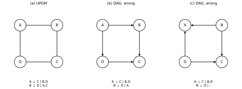
fig_4_37. Reproduces Murphy (2023), Figure 4.37. Download: PDF · SVG4.5.2 Converting between a directed and undirected model
4.5.2.1 Converting a DPGM to a UPGM
pp. 196–197, (4.149)–(4.152), Figure 4.38 Moralise, then drop arrows. For the full student network with \(C\) (coherence) and \(H\) (happiness), \(J\) (job), the joint is \[ p(C)p(D\given C)p(I)p(G\given I,D)p(S\given I)p(L\given G)p(J\given L,S)p(H\given G,J) \] (4.150) and moralisation adds the edges \(D-I\), \(G-J\) and \(L-S\) (the co-parents of \(G\), \(H\) and \(J\)). Each CPD becomes a factor on a clique (its family is a clique after moralisation), all potentials are locally normalised and \(Z=1\) (4.151)–(4.152). Safety: the resulting UPGM is an I-map of the DPGM (Result 8.15); but it asserts fewer independences. Over 120 random DAGs, 104 independences of the DAGs that the moral graph misses were found among the random queries, and no separation of the moral graph was ever absent from the DAG.
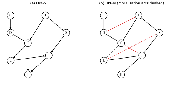
fig_4_38. Reproduces Murphy (2023), Figure 4.38. Download: PDF · SVG4.5.2.2 Converting a UPGM to a DPGM
Filling the gap 4.21: the dummy-child construction p. 197, Figure 4.39
The book converts an undirected model to a directed one by adding, for each potential \(\psi_c\), an observed dummy child \(Y_c=y_c^*\) with \(p(Y_c=y_c^*\given x_c)=\psi_c(x_c)\), and states that "\[ p_{\mathrm{undir}}(\mathbf{x})\propto p_{\mathrm{dir}}(\mathbf{x},\mathbf{y}^*) \]".
Derivation
Two conditions are implicit. First, \(p(Y_c=y^*\given x_c)\) must be at most 1, so \(\psi_c\) is first divided by \(\max\psi_c\), which only changes \(Z\). Second, the parent nodes \(\mathbf{x}\) need a prior; take the uniform one (a constant), or absorb the prior into one of the potentials. Then \[ p_{\mathrm{dir}}(\mathbf{x},\mathbf{Y}=\mathbf{y}^*)=p_0(\mathbf{x})\prod_c\psi_c(x_c)/\max\psi_c\propto\prod_c\psi_c(x_c) \], and conditioning on the observed dummies gives \[ p_{\mathrm{dir}}(\mathbf{x}\given\mathbf{y}^*)=p_{\mathrm{undir}}(\mathbf{x}) \] exactly. The observed child of \(x_c\) is a collider with observed descendant, so by Result 4.3 it makes all the members of \(c\) dependent, as in the clique of the UPGM. (Checked numerically on a random positive 4-variable potential.)
4.5.3 Conditional directed vs undirected PGMs and the label bias problem
pp. 197–198, Figures 4.40–4.41 The chain CRF (undirected) and the MEMM (directed, locally normalised) behave differently in the discriminative setting. In the MEMM \(y_{t-1}\indep x_t\given y_t\) for the posterior, "blocking information flow backwards in time"; the CRF, globally normalised, does not have this problem. In the part-of-speech example, "banks" may be a verb or a noun; a later word "fishing" should settle it, but in an MEMM it cannot reach the tag of "banks".
Filling the gap 4.22: why local normalisation blocks the backward flow of evidence p. 198
The book asserts \(y_{t-1}\indep x_t\given y_t\). Here is the argument, and a numerical contrast.
Derivation
In an MEMM, \[ p(\mathbf{y}\given\mathbf{x})=p(y_1\given x_1)\prod_{t\ge2}p(y_t\given y_{t-1},x_t) \] and each conditional sums to 1 over \(y_t\). Sum out \(y_T\), then \(y_{T-1}\), and so on: each sum over a node with no remaining dependants equals 1 regardless of \(x_t\). Hence \[ p(y_{1:s}\given\mathbf{x})=p(y_1\given x_1)\prod_{t=2}^sp(y_t\given y_{t-1},x_t) \] does not depend on \(x_{s+1},\dots,x_T\): later observations cannot change beliefs about earlier labels. In a CRF the factor \(Z(\mathbf{x})\) and the sums over later labels are not 1; \(\sum_{y_t}\psi(y_{t-1},y_t)\psi(y_t,x_t)\) depends on \(x_t\), so the marginal of \(y_{t-1}\) does depend on later observations. Numbers. Two tags, \(\phi_1=(0,0)\) for the ambiguous first word, edge scores \[ \psi=\begin{pmatrix}2&0\\0&2\end{pmatrix} \] (tags tend to agree) and node scores \((3,0)\) or \((0,3)\) for the second word. The CRF gives \(p(y_1=0\given x_1,x_2)=0.845\) or \(0.155\); the MEMM with the same scores gives \(0.5\) in both cases. In a random 5-position example the first marginal of the CRF moves noticeably when the adjacent observation's scores are changed by \(\pm4\), whereas the MEMM's is unchanged to \(10^{-12}\). The price of global normalisation, as the book says, is that there is no valid distribution over \(y_{1:T}\) before the whole sentence is seen, and training needs \(Z\) for every example.
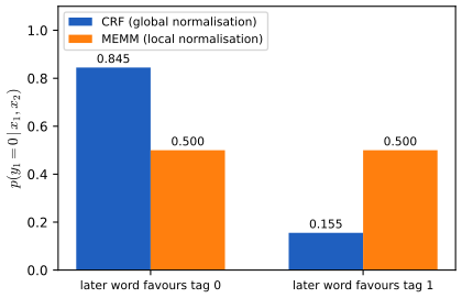
fig_4_S3. Download: PDF · SVG4.5.4 Combining directed and undirected graphs
pp. 198–200, (4.153)–(4.156), Figures 4.41–4.43 Chain graphs have directed and undirected edges but no directed cycles; the denoising model (4.153) has an undirected prior and a directed likelihood. A partially directed acyclic graph decomposes into chain components (connected by undirected edges) arranged in a DAG; the joint is \(\prod_ip(C_i\given\pa(C_i))\) with each factor a CRF (4.154)–(4.156), e.g. \[ p(C,D,E\given A,B)=Z(A,B)^{-1}\phi(A,C)\phi(B,E)\phi(C,D)\phi(D,E) \]. A latent-variable DAG can be projected so that each latent variable is a root with exactly two observed children (Pearl, 2009); replacing each by a bidirected edge gives an acyclic directed mixed graph (ADMG), whose independences are read by m-separation, d-separation after replacing \(Y_i\leftrightarrow Y_j\) by \(Y_i\leftarrow X_{ij}\to Y_j\); the linear-Gaussian case is the structural equation model of Section 4.7.2.
4.5.5 Comparing directed and undirected Gaussian PGMs
pp. 200–202, (4.157)–(4.159), Figures 4.44–4.45 Directed GGMs have sparse regression matrices \(\mathbf{W}\), undirected ones sparse precision matrices (Result 4.2, Result 4.8). The advantage of the directed form is that \(\mathbf{W}\), and so \(\bm\Sigma\), can depend on covariates without any positive-definiteness constraint (for any \(\mathbf{W}\) and positive \(\mathbf{S}\), \(\bm\Sigma=\mathbf{U}\mathbf{S}^2\mathbf{U}^\T\) is positive definite since \(\mathbf{U}\) is invertible); the disadvantage is its dependence on the node order. A combination is the Gaussian chain graph, e.g. a vector autoregression of order 2 (VAR(2)), \[ p(\mathbf{x}_t\given\mathbf{x}_{t-1},\mathbf{x}_{t-2})=\N(\mathbf{A}_1\mathbf{x}_{t-1}+\mathbf{A}_2\mathbf{x}_{t-2},\bm\Sigma) \] (4.157), with directed arcs between slices from the non-zeros of \(\mathbf{A}_1,\mathbf{A}_2\) and undirected arcs within a slice from the non-zeros of \(\bm\Sigma^{-1}\).
Filling the gap 4.23: the VAR example, and sparse covariance versus sparse precision pp. 200–202, (4.158)–(4.159)
The book prints \(\bm\Sigma\) and \(\bm\Sigma^{-1}\) with two decimals and draws the graph; the matrices behind the example and the covariance-graph statement need justification.
Derivation
The \(3\times3\) block of \(\bm\Sigma\) in (4.159) is \[ \begin{pmatrix}1&\tfrac12&\tfrac13\\\tfrac12&1&-\tfrac13\\\tfrac13&-\tfrac13&1\end{pmatrix} \] (the other two nodes are independent, with unit variance). Its inverse has exact entries \(\tfrac{32}{15}=2.133\), \(-\tfrac{22}{15}=-1.467\), \(-\tfrac65\), \(\tfrac65\), \(\tfrac95\), which round to the printed 2.13, \(-1.47\), \(-1.2\), 1.2, 1.8. The zeros in \(\bm\Sigma^{-1}\) are the missing within-slice undirected edges (nodes 4 and 5 have none), while the zero pattern of \(\mathbf{A}_1\) and \(\mathbf{A}_2\) (as read off the page: \(\mathbf{A}_1\) has 11 non-zeros, \(\mathbf{A}_2\) has 4) gives the missing directed arcs; Figure 4.44 is drawn from exactly these matrices.
Covariance graphs. A bidirected graph where an absent edge means marginal independence: in the Gaussian case \(\Sigma_{13}=0\) means \(Y_1\indep Y_3\), whereas the undirected model with a missing 1–3 edge means \(\Lambda_{13}=0\) and \(Y_1\indep Y_3\given Y_2\) (a chain \(1-2-3\) has \(\Lambda_{13}=0\) but \(\Sigma_{13}\ne0\), as in the demonstration). A bidirected edge corresponds to a hidden common cause: the DAG of Figure 4.45(b) with latent confounders \(Z_1,Z_2\) between \(Y_1,Y_2\) and \(Y_2,Y_3\) has \(Y_1\indep Y_3\) (no connecting path unless \(Y_2\) is observed as a collider) and \(Y_1\nindep Y_3\given Y_2\).
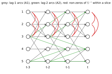
fig_4_44. Reproduces Murphy (2023), Figure 4.44 (redrawn from the printed matrices; the original is a figure taken from the literature). Download: PDF · SVG4.6 PGM extensions
4.6.1 Factor graphs
pp. 202–205, (4.160)–(4.166), Figures 4.46–4.49 A factor graph is a bipartite graph of variable nodes (round) and factor nodes (square), with an edge from each variable to every factor that mentions it; it represents a function \(f(\mathbf{x})=\prod_af_a(\mathbf{x}_a)\). The MRF of Figure 4.46(a) with one potential per maximal clique gives \(f_{124}(x_1,x_2,x_4)f_{234}(x_2,x_3,x_4)\) (4.160); one potential per edge gives \(f_{14}f_{12}f_{34}f_{23}f_{24}\) (4.161), a finer description of the same graph. A DPGM becomes a factor graph by one factor per CPD, e.g. \[ f_1(x_1)f_2(x_2)f_{123}(x_1,x_2,x_3)f_{34}f_{35} \] (4.162) with \(f_{123}=p(x_3\given x_1,x_2)\); when each node has at most one parent (chains and trees) there is one factor per edge and the model is a pairwise MRF. In a Forney (normal) factor graph nodes are factors and edges are variables (4.163); a variable used by more than two factors needs an equality node \(f_=(x,x_1,x_2)=\delta(x-x_1)\delta(x-x_2)\) (4.165), so that \[ f(x,y_1,y_2)=f_x(x)f_{y\given x}(y_1,x)f_{y\given x}(y_2,x) \] (4.166); FFGs compose hierarchically, e.g. \[ f_{\mathrm{prior}}(x_1,\dots,x_4)f_{\mathrm{lik}}(x_4,x_5) \] (4.164), and are the usual form for message-passing decoders of error-correcting codes. Message passing on them is Chapter 9.
4.6.2 Probabilistic circuits
pp. 205–206 A sum-product network (SPN; Poon and Domingos, 2011) is a directed tree-like graph whose leaves are univariate distributions and whose internal nodes are weighted sums (mixtures) and products; it is a deep mixture model, and context-specific independence lets exact inference cost the number of links rather than the treewidth. Einsum networks (Peharz et al., 2020) connect them to tensor contractions.
Filling the gap 4.24: why an SPN is a distribution with linear-time marginals p. 205
The book describes SPNs without a definition of validity. Call a sum node complete if all its children have the same scope (set of variables) and a product node decomposable if its children have pairwise disjoint scopes; take non-negative sum weights summing to 1.
Derivation
Claim: every node with scope \(S\) computes a normalised distribution of \(\mathbf{x}_S\), and replacing the leaf distributions of the variables in a subset \(M\) by the constant 1 returns the marginal over \(S\setminus M\). By induction on the structure. Leaves: a univariate distribution sums to 1, and setting it to 1 marginalises it. A product of children with disjoint scopes \(S_1,\dots,S_m\) is \(\prod_jp_j(\mathbf{x}_{S_j})\), the joint of independent blocks, normalised, and marginalisation distributes over the factors since the scopes are disjoint. A complete sum \(\sum_jw_jp_j(\mathbf{x}_S)\) with \(\sum w_j=1\) is a mixture, normalised, and summing a variable in \(S\) out of the mixture is the mixture of the marginals. So one bottom-up pass of cost linear in the number of edges evaluates a probability or any marginal. A tiny network \[ 0.3\,\mathrm{Ber}(x_1;0.9)\mathrm{Ber}(x_2;0.2)+0.7\,\mathrm{Ber}(x_1;0.1)\mathrm{Ber}(x_2;0.6) \] sums to 1 over the four states, and \(p(x_1=1)=0.3\cdot0.9+0.7\cdot0.1=0.34\) is obtained by setting the \(x_2\) leaves to 1 (verified). This is the same cost-saving idea as the barren-node and variable-elimination arguments, but with the independences coded in the structure of the circuit.
4.6.3 Directed relational PGMs
pp. 206–208, (4.167)–(4.175), Figures 4.50–4.51 A fixed Bayes net cannot express models whose repeated structure depends on the objects present (not even an HMM is expressible with plates). A relational probability model has objects, functions with type signatures and predicates. The book's book-review example has customers and books with \(H:\mathrm{Customer}\to\{T,F\}\) (honest), \(K\) (kindness, 1–5), \(Q:\mathrm{Book}\to\{1..5\}\) (quality) and \[ R:\mathrm{Customer}\times\mathrm{Book}\to\{1..5\} \] (rating), with priors \(H(c)\sim\mathrm{Cat}(0.99,0.01)\) (4.171), (4.172), (4.173) and a CPD \(R(c,b)\sim\mathrm{RecCPD}(H(c),K(c),Q(b))\) (4.174). Instantiating the template for \(C\) customers and \(B\) books gives a ground network.
Filling the gap 4.25: size of the ground network and of the CPD p. 206
Derivation
The ground variables are \(H(c)\) and \(K(c)\) for each customer (\(2C\)), \(Q(b)\) for each book (\(B\)) and \(R(c,b)\) for each pair (\(CB\)): \(CB+2C+B\) variables in all (22 for \(C=3\), \(B=4\)). The number of possible worlds is the product of the state counts, \(2^C\cdot5^C\cdot5^B\cdot5^{CB}=2^C5^{C+B+BC}\) (the book's "\(2C5C+B+BC\)" has lost its exponents). A RecCPD table has one row per joint configuration of its three parents, \(2\times5\times5=50\) rows of 5 entries. With identity uncertainty the rating depends on the whole vector \(Q(1{:}B)\) and a selector \(L(c)\), acting as a multiplexer: \(R(c,b)\sim\mathrm{RecCPD}(H(c),K(c),Q(b'))\), \(b'=L(c)\) (4.175); this is a mixture over which parent is active, so a node with \(B\) potential parents needs only the table of one. Dynamic unrolling instantiates only the part of the ground network relevant to a query.
4.6.4 Undirected relational PGMs
pp. 208–211, (4.176)–(4.182), Figure 4.52, Table 4.5 The undirected analogue is natural for discriminative problems, as for CRFs: collective classification of web pages uses a template CRF over the link structure with tied parameters. Markov logic networks (MLNs) attach a weight to each first-order rule. The rules "Smoking causes cancer", \(\forall x.\,Sm(x)\Rightarrow Ca(x)\) (4.176), and "friends of smokers smoke", \[ \forall x,y.\,Fr(x,y)\wedge Sm(x)\Rightarrow Sm(y) \] (4.177), have clausal forms \(\neg Sm(x)\vee Ca(x)\) and \(\neg Fr(x,y)\vee\neg Sm(x)\vee Sm(y)\) (4.178)–(4.179). With two people (A, B) there are eight ground atoms and \(2^8\) worlds; a hard potential gives 1 if the clause holds and 0 otherwise (4.180), a soft one \(e^w\) or \(e^0\) (4.181), and the joint is
\[ p(\mathbf{x})=\frac{1}{Z(\mathbf{w})}\exp\Big(\sum_iw_in_i(\mathbf{x})\Big), \tag{4.182} \]where \(n_i\) counts the true groundings of clause \(i\).
Filling the gap 4.26: the MLN with two people, and the size of an unrolled undirected model pp. 209–211
The book defines the model and then asserts that the size of an unrolled undirected model changes inference even when no new evidence is added. Here are the numbers.
Derivation
The MLN. Each grounding of a clause contributes a potential \(e^{w}\) when satisfied and 1 otherwise, so the product of potentials over groundings is \(\exp(\sum_iw_in_i)\), (4.182). With weights \(w_1\) (for the cancer rule, 2 groundings) and \(w_2\) (for the friendship rule, 4 groundings) the eight atoms Fr(A,A), Fr(A,B), Fr(B,A), Fr(B,B), Sm(A), Sm(B), Ca(A), Ca(B) give 256 worlds. For \(w_1=w_2=0\) the distribution is uniform. Exactly 112 worlds satisfy all six groundings; as \(w_1,w_2\to\infty\) the distribution tends to the uniform distribution on those 112 worlds (hard constraints), confirmed by counting and by \(w=12\). The probability \(p(Ca(A)\given Sm(A))\) is \(\tfrac12\) at \(w_1=0\) and increases towards 1 as \(w_1\) grows: the weight measures how strongly the rule is enforced, and "smoking does not always cause cancer" is a finite weight. Inference on the ground network uses the usual methods, with lifted inference avoiding the grounding.
Unrolling. Consider an undirected chain \(z_1-\cdots-z_n\) with edge potential \(\psi(z_t,z_{t+1})\) and evidence only on the first \(T\) nodes (model M1 has \(n=T\); model M2 extends it to \(n=2T\) with no new evidence). Marginalising the extra nodes out of M2 multiplies the weight of \(z_T\) by \[ m(z_T)=\sum_{z_{T+1}}\psi(z_T,z_{T+1})\sum_{z_{T+2}}\psi(z_{T+1},z_{T+2})\cdots \], which is a function of \(z_T\) unless the rows of \(\psi\) have equal sums. Since \(\psi\) is not a conditional probability, in general \(m\) is not constant and the posterior of \(z_t\) given \(y_{1:T}\) changes. In a directed chain every conditional sums to 1, so the same marginalisation gives \(m\equiv1\) and the added nodes have no effect (they are barren). Example: \(T=2\), \[ \psi=\begin{pmatrix}4&1\\0.5&1\end{pmatrix} \], likelihoods \((0.7,0.2)\) and \((0.3,0.6)\): \(p(z_1=0\given y_{1:2})=0.8936\) in M1 and \(0.9461\) in M2, whereas with the row-normalised \(\psi\) (a directed chain) both equal 0.7664. This is the sense in which locally normalised models are modular.
4.6.5 Open-universe probability models
pp. 211–212 Relational models assume a closed world with a known set of objects. In open-universe models (OUPMs) the number of objects and their identities are uncertain (an unknown number of aircraft to track, seismic events, matching citations); the first formal language was BLOG (Milch et al., 2005), and other languages and libraries support efficient inference. No new equations are introduced here.
4.6.6 Programs as probability models
pp. 211–212 In a probabilistic programming language the set of possible worlds is the set of execution traces of a program with two extra constructs: random draws (which define \(p(z,y)\)) and conditioning on observations (which gives \(p(z\given y)\)) (Gordon et al., 2014); inference is often by sequential Monte Carlo (Chapter 13) or MCMC. This is the procedural counterpart of the declarative OUPM.
4.7 Structural causal models
pp. 212–217, (4.183)–(4.192), Figures 4.53–4.55, Table 4.6 A structural causal model (SCM) is a triple \(M=(U,V,F)\): exogenous noise variables \(U_i\), endogenous variables \(V_i\), and deterministic mechanisms \(V_i=f_i(V_{\pa_i},U_i)\) whose dependency graph is a DAG. If the \(U_i\) are independent the SCM is Markovian; dependent noises (a bidirected edge) give a semi-Markovian SCM. Pushing the noise through the mechanisms induces a distribution over \(V\) like a PGM, but with stronger assumptions. The causal chapter of the book is Chapter 36; the companion treatments are Theorem 17.E, Theorem 17.F and Chapter 16.
4.7.1 Example: causal impact of education on wealth
Let \(X\) be education, \(Z\) debt and \(Y\) wealth, with \(X\to Z\), \(X\to Y\), \(Z\to Y\) (Figure 4.53). The SCM is \(X=f_X(U_x)\), \(Z=f_Z(X,U_z)\), \(Y=f_Y(X,Z,U_y)\) (4.183)–(4.185), and the PGM it induces is \(p(X)p(Z\given X)p(Y\given X,Z)\).
4.7.2 Structural equation models
A structural equation model (SEM, path diagram) has linear mechanisms and Gaussian noise: \(X=U_x\), \(Z=c_z+w_{xz}X+U_z\), \(Y=c_y+w_{xy}X+w_{zy}Z+U_y\) (4.186)–(4.188), equivalent to the Gaussian DGM \(p(X)=\N(\mu_x,\sigma_x^2)\), \(p(Z\given X)=\N(c_z+w_{xz}X,\sigma_z^2)\), \[ p(Y\given X,Z)=\N(c_y+w_{xy}X+w_{zy}Z,\sigma_y^2) \] (4.189)–(4.191) (read the noise term as a Gaussian variable, \(U_z\sim\N(0,\sigma_z^2)\); the book's \(p(U_z)=\N(U_x\given0,\sigma_z^2)\) and \(p(U_y)=\N(U_x\given\cdots)\) reuse the symbol \(U_x\) by mistake). Nonparametric SEMs are SCMs.
4.7.3 Do operator and augmented DAGs
A perfect intervention \(\mathrm{do}(X_i=x_i)\) clamps the variable and cuts its incoming edges ("graph surgery", Figure 4.54a); an additive intervention replaces \(Z=f_Z(X,U_z)\) by \(f_Z+\Delta\); the augmented DAG adds an action node \(A_z\in\{0,1\}\) as a parent (4.192).
Result 4.13 (seeing is not doing) pp. 214–215, (4.183)–(4.192)
In the Markovian SCM of (4.183)–(4.185): (a) the joint is \(p(x)p(z\given x)p(y\given x,z)\). (b) After \(\mathrm{do}(Z=z)\), \[ p(x,y\given\mathrm{do}(Z=z))=p(x)p(y\given x,z) \] (truncated factorisation); so \(p(X\given\mathrm{do}(Z=z))=p(X)\), whereas \(p(X\given Z=z)\ne p(X)\) in general, and \[ p(y\given\mathrm{do}(Z=z))=\sum_xp(x)p(y\given x,z) \], which differs from \(p(y\given z)=\sum_xp(x\given z)p(y\given x,z)\). (c) In the augmented DAG, \[ p(Q\given\mathrm{do}(A_z=a),E=e)=p(Q\given A_z=a,E=e) \], because \(A_z\) has no parents and so there are no edges to cut. (d) In the linear Gaussian SEM, \[ \mathbb{E}[Y\given\mathrm{do}(Z=z)]=c_y+w_{xy}\mathbb{E}[X]+w_{zy}z \], but the observational regression slope of \(Y\) on \(Z\) is \[ w_{zy}+w_{xy}\mathrm{Cov}(X,Z)/\mathrm{Var}(Z) \].
Proof
(a) The noises are independent, so each variable is a function of its parents and an independent noise: that is a Bayes net with the CPDs induced by the mechanisms. (b) Replacing the mechanism of \(Z\) by \(Z=z\) deletes the factor \(p(z\given x)\) from the joint and fixes \(z\) in the others: the surviving factors are \(p(x)\) and \(p(y\given x,z)\). Marginalising gives the two statements; \(X\) is not a descendant of \(Z\) so intervening on \(Z\) cannot change it. In contrast \(p(x\given z)\propto p(x)p(z\given x)\) depends on \(z\) whenever \(Z\) depends on \(X\). (c) \(p(Q\given A_z=a,E=e)\) is ordinary conditioning in the augmented joint, which has the new mechanism for \(Z\) selected by \(a\); setting an exogenous parent changes the mechanism and nothing else. (d) The first expression follows from (b). For the second, \[ \mathrm{Cov}(Z,Y)=w_{zy}\mathrm{Var}(Z)+w_{xy}\mathrm{Cov}(Z,X) \] since \(U_y\) is independent of \(X,Z\); divide by \(\mathrm{Var}(Z)\). ∎
In the example the book describes (pay off everyone's debt), \(p(X\ge1\given Z=0)\) is small (someone with no debt probably did not go to college) but \(p(X\ge1\given\mathrm{do}(Z=0))=p(X\ge1)\). Numerically, with \(\mu_x=1,\sigma_x=1\), \(w_{xz}=1.5\), \(\sigma_z=0.5\), \(w_{xy}=2\), \(w_{zy}=-1\), \(\sigma_y=0.5\): the observational slope of \(Y\) on \(Z\) is \(+0.20\) (more debt, apparently more wealth, because both reflect education), but the causal slope is \(-1\). In a simulation of two million cases the observational slope is \(0.2000\); under \(\mathrm{do}(Z=2)\) the mean of \(Y\) is \(c_y+w_{xy}\cdot1-2=1\) as predicted and the mean of \(X\) stays at 1, whereas among cases with \(Z\approx2\) the mean of \(X\) is 1.30. This is a confounding (omitted-variable) bias.
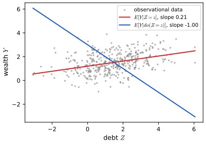
fig_4_S4. Download: PDF · SVG4.7.4 Counterfactuals
pp. 215–217, Table 4.6, Figure 4.55 Pearl's causal hierarchy has three levels: association \(p(Y\given a)\) (seeing), intervention \(p(Y\given\mathrm{do}(a))\) (doing) and counterfactuals \(p(Y^{a'}\given\mathrm{do}(a),y')\) (imagining). The potential outcome \(Y^{a'}\) is the outcome that would occur had action \(a'\) been taken. The book states that counterfactual reasoning needs strictly more assumptions than interventional reasoning. For a unit with exogenous noise \(U_i\), counterfactuals are computed by abduction (infer \(p(U_i\given A_i=a,Y_i=y)\)), action (replace \(A_i=a\) by \(a'\)) and prediction (push the posterior of \(U_i\) through the modified model). The potential-outcomes framework is the same SCM under SUTVA (units independent), shared mechanisms and noise unaffected by actions; both outcomes \(Y_i^0,Y_i^1\) exist but only one is observed (the fundamental problem of causal inference); twin networks clone the deterministic part.
Result 4.14 (counterfactuals are not determined by the interventional distribution) p. 216
Let \(A\in\{0,1\}\) be a treatment and \(Y^a=\ind(U<p_a)\) for \(U\sim\mathrm{Unif}(0,1)\) (a monotone coupling) with \(p_0<p_1\). Then \(\Pr(Y^0=1\given A=1,Y=1)=p_0/p_1\). A second SCM, \(Y^1=\ind(U<p_1)\) and \(Y^0=\ind(U>1-p_0)\) (antitone coupling), has the same interventional distributions \(\Pr(Y^a=1)=p_a\) but \[ \Pr(Y^0=1\given A=1,Y=1)=\max(0,p_0+p_1-1)/p_1 \]. So the interventional distribution does not determine the counterfactual.
Proof
Abduction: given \(A=1\) and \(Y=1\) (with \(A\) independent of \(U\) by randomisation) the posterior of \(U\) is uniform on \((0,p_1)\). Action and prediction in the first SCM: \(Y^0=1\) iff \(U<p_0\), which has probability \(p_0/p_1\) on \((0,p_1)\) (as \(p_0<p_1\)). In the second, \(Y^0=1\) iff \(U>1-p_0\); the overlap of \((1-p_0,1)\) with \((0,p_1)\) has length \(\max(0,p_0+p_1-1)\). Both SCMs give \(\Pr(Y^a=1)=p_a\) since \(\Pr(U<p_1)=p_1\) and \(\Pr(U>1-p_0)=p_0\), and the data (which reveal only one of \(Y^0,Y^1\) per unit) cannot tell them apart. ∎
For \(p_0=0.3\), \(p_1=0.6\) the two answers are \(0.5\) and \(0\) (confirmed by simulating two million units with each coupling): in the first model half of the treated, cured patients would have been cured anyway, in the second none would. The linear case is simpler: in \(Y=2X+U\), observing \((X=1,Y=3)\) gives \(U=1\) and so, had \(X\) been 0, \(Y\) would have been \(1\). Section 29.12.6 of the book gives a time-series application (the counterfactual impact of an intervention).
Practice problems
Chapter 4 of the book has no end-of-chapter exercises. Here are three short problems with worked solutions.
Problem 4.1. In the student network show that \(D\) and \(S\) are marginally independent, that they are still independent given \(\{L,I\}\), but dependent given \(L\) alone.
Solution
The only path from \(D\) to \(S\) is \(D\to G\leftarrow I\to S\) (and \(G\to L\) is a dead end). The collider \(G\) blocks it unless \(G\) or a descendant is observed. Marginally nothing is observed, so \(D\indep S\). Given \(\{L,I\}\) the node \(I\) is observed and is a non-collider on the path (a fork \(G\leftarrow I\to S\)), so the path is blocked: \(D\indep S\given\{L,I\}\) (this is in Table 4.1). Given \(L\) alone the collider \(G\) has the observed descendant \(L\), and \(I\) is not observed, so the path is open: \(D\nindep S\given L\). Numerically \(I(D;S\given L)=0.0035\) nats, while the other two mutual informations are zero to rounding error. The dependence is weak because \(L\) is a noisy function of \(G\).
Problem 4.2. An Ising chain \(x_1-x_2-\cdots-x_n\) (open ends, no field) has weight \(e^{Jx_ix_{i+1}}\) per edge. Show that \(\mathbb{E}[x_ix_{i+1}]=\tanh J\) and \(\mathbb{E}[x_1x_n]=(\tanh J)^{n-1}\). Why is the covariance dense although the graph is a chain?
Solution
Substitute \(b_i=x_ix_{i+1}\in\{\pm1\}\), \(i=1,\dots,n-1\): the map \((x_1,\dots,x_n)\mapsto(x_1,b_1,\dots,b_{n-1})\) is a bijection, the weight is \(\prod_ie^{Jb_i}\) and does not involve \(x_1\), so the \(b_i\) are independent with \[ \mathbb{E}b_i=(e^J-e^{-J})/(e^J+e^{-J})=\tanh J \]. Then \(x_1x_n=b_1\cdots b_{n-1}\) has expectation \((\tanh J)^{n-1}\). Every pair is correlated (with correlation \((\tanh J)^{|i-j|}\), decaying geometrically) although non-neighbours are conditionally independent given the nodes between them: the same mechanism as the AR(1) covariance of Result 4.8. A direct enumeration for \(J=0.7\), \(n=2,3,4\) gives 0.6044, 0.3653, 0.2208 as predicted.
Problem 4.3. In the collider \(x,y\sim\N(0,1)\) independent and \(z\given x,y\sim\N(x+y,s^2)\), find \(\mathrm{corr}(x,y\given z)\), and its limit as \(s\to0\) and \(s\to\infty\).
Solution
The posterior precision of \((x,y)\) given \(z\) is the prior precision \(\mathbf{I}\) plus the likelihood term \(s^{-2}\mathbf{1}\mathbf{1}^\T\), i.e. \[ \begin{pmatrix}1+s^{-2}&s^{-2}\\s^{-2}&1+s^{-2}\end{pmatrix} \]. Its inverse has off-diagonal entry proportional to \(-s^{-2}\) and diagonal proportional to \(1+s^{-2}\), so \(\mathrm{corr}=-s^{-2}/(1+s^{-2})=-1/(1+s^2)\), the same for every \(z\) (checked: \(-0.5\) for \(s=1\), \(-0.8\) for \(s=0.5\)). As \(s\to0\) (\(z=x+y\) exactly) the correlation tends to \(-1\); as \(s\to\infty\) the observation is uninformative and it tends to 0. This is the Gaussian version of explaining away.
Demonstrations for this chapter
Each demonstration runs in the browser, with seeded random numbers so that a class sees the same pictures, and links back to these notes. The ▶ Demo boxes above open them already set to the case under discussion. Their exact quantities (posterior marginals, correlations, precision matrices, exact enumerations of the \(4\times4\) lattice and the mean-field iterates) are the numbers of the Python code.
| Demonstration | What you can see | Sections and results |
|---|---|---|
| Inference and d-separation in a Bayes net | Exact posteriors in the student and sprinkler networks as evidence is added; a d-separation tester against the exact mutual information; selection in a Gaussian collider. Presets: 1 grade C; 2 also SAT good; 3 observe the letter; 4 wet grass; 5 sprinkler on; 6 select z>2.5; 7 weak selection. | 4.2.4, 4.2.6; Filling the gaps 4.1, 4.2, 4.6; Result 4.3 |
| Gaussian Bayes nets and Gaussian MRFs | A linear-Gaussian DAG with its precision (sparse, the moral graph) and covariance (dense) as heat maps; click a pair to compare marginal and conditional dependence. Presets: 1 AR(1); 2 v-structure; 3 chain; 4 fork; 5 Figure 4.23; 6 AR(1), rho = 0.9. | 4.2.3, 4.3.5, 4.5.5; Results 4.2, 4.8 |
| Ising and Potts models: Gibbs sampling and denoising | Checkerboard Gibbs sampling as the coupling crosses the critical value, with Onsager's curve and exact 4 × 4 numbers; mean-field denoising with an Ising prior. Presets: 1 J = 0.2; 2 J = 0.44; 3 J = 0.6 ordered; 4 J = 3; 5 antiferromagnet; 6 field; 7 Potts below; 8 Potts above; 9 denoise; 10 J = 0; 11 J = 2. | 4.3.2, 4.3.8; Filling the gaps 4.8, 4.9, 4.16 |
The Python code that produces every figure of this page is code/ch04_graphical_models.py (see the code index).
Errors and slips found in the book
Everything below was confirmed by recomputation. Items marked (minor) are notational.
- Section 4.2.6.1: "\(p(D=\text{Hard}\given G=C)=0.76\)" should read \(p(D=\text{Hard}\given G=C,S=\text{Good})\); given \(G=C\) alone it is 0.63 (Filling the gap 4.1).
- (4.107): the printed covariance of the AR(1) example is not the inverse of (4.106); the correct one is \(\tau^2\rho^{|i-j|}/(1-\rho^2)\) (box above).
- (4.104): the partition function of the Gaussian MRF with a linear term is missing the factor \[ \exp(\tfrac12\bm\eta^\T\bm\Lambda^{-1}\bm\eta) \].
- Below (4.128): "for Gaussian MRFs PL is equivalent to ML" holds for the saturated model only (Filling the gap 4.18).
- Section 4.4.1.1: the printed potential that is set to 0 to encode "B must precede I" forbids the wrong transitions (box above); also OBIOBIO is not an example of adjacent chunks.
- Supplement (4.19): the Gaussian RBM energy is printed with \(-\tfrac12\sum_d(x_d-b_d)^2\); with that sign \(e^{-E}\) grows in \(x\) and cannot be normalised. The sign of the quadratic term must be positive, \(+\tfrac12\sum_d(x_d-b_d)^2\), which is what the conditional (4.21) \(\N(b_d+\sum_kw_{dk}z_k,1)\) requires (Filling the gap 4.12). The hidden bias is written \(a_k\) in (4.19) and \(c_k\) in (4.22) (minor).
- (4.3): the second form of the first-order Markov joint is printed with \(p(x_t\given x_{1:t-1})\) (the chain rule) rather than \(p(x_t\given x_{t-1})\) (minor). Below (4.71): the energy is said to be positive, which is unnecessary (minor). Section 4.7.2: the Gaussian noise densities reuse the symbol \(U_x\) for all three noise terms (minor).
References
- Murphy, K. P. (2023). Probabilistic Machine Learning: Advanced Topics. MIT Press. Chapter 4 (pp. 143–217) and Supplementary Chapter 4. probml.github.io/pml-book/book2.html.
- Amit, D. J., Gutfreund, H. and Sompolinsky, H. (1985). Storing infinite numbers of patterns in a spin-glass model of neural networks. Physical Review Letters, 55, 1530–1533.
- Baxter, R. J. (1973). Potts model at the critical temperature. Journal of Physics C, 6, L445–L448.
- Beffara, V. and Duminil-Copin, H. (2012). The self-dual point of the two-dimensional random-cluster model is critical for \(q\ge1\). Probability Theory and Related Fields, 153, 511–542.
- Besag, J. (1975). Statistical analysis of non-lattice data. The Statistician, 24, 179–195.
- Della Pietra, S., Della Pietra, V. and Lafferty, J. (1997). Inducing features of random fields. IEEE Transactions on Pattern Analysis and Machine Intelligence, 19(4), 380–393.
- Felzenszwalb, P. F., Girshick, R. B., McAllester, D. and Ramanan, D. (2010). Object detection with discriminatively trained part-based models. IEEE Transactions on Pattern Analysis and Machine Intelligence, 32(9), 1627–1645.
- Friedman, N., Geiger, D. and Goldszmidt, M. (1997). Bayesian network classifiers. Machine Learning, 29, 131–163.
- Gordon, A. D., Henzinger, T. A., Nori, A. V. and Rajamani, S. K. (2014). Probabilistic programming. Future of Software Engineering.
- Haldane, J. B. S. (1919). The combination of linkage values and the calculation of distances between the loci of linked factors. Journal of Genetics, 8, 299–309.
- Hopfield, J. J. (1982). Neural networks and physical systems with emergent collective computational abilities. Proceedings of the National Academy of Sciences, 79, 2554–2558.
- Koller, D. and Friedman, N. (2009). Probabilistic Graphical Models. MIT Press.
- Lafferty, J., McCallum, A. and Pereira, F. (2001). Conditional random fields: probabilistic models for segmenting and labeling sequence data. ICML.
- Lauritzen, S. L. and Spiegelhalter, D. J. (1988). Local computations with probabilities on graphical structures and their application to expert systems. Journal of the Royal Statistical Society B, 50, 157–224.
- Marks, T. K. and Movellan, J. R. (2001). Diffusion networks, products of experts, and factor analysis. Proceedings of the 3rd International Conference on Independent Component Analysis and Signal Separation.
- Milch, B., Marthi, B., Russell, S., Sontag, D., Ong, D. L. and Kolobov, A. (2005). BLOG: probabilistic models with unknown objects. IJCAI.
- Neal, R. M. (1992). Connectionist learning of belief networks. Artificial Intelligence, 56, 71–113.
- Onsager, L. (1944). Crystal statistics. I. A two-dimensional model with an order-disorder transition. Physical Review, 65, 117–149.
- Pearl, J. (2009). Causality, 2nd edition. Cambridge University Press.
- Peharz, R., Lang, S., Vergari, A., Stelzner, K., Molina, A., Trapp, M., Van den Broeck, G., Kersting, K. and Ghahramani, Z. (2020). Einsum networks: fast and scalable learning of tractable probabilistic circuits. ICML.
- Poon, H. and Domingos, P. (2011). Sum-product networks: a new deep architecture. UAI.
- Potts, R. B. (1952). Some generalized order-disorder transformations. Proceedings of the Cambridge Philosophical Society, 48, 106–109.
- Richardson, M. and Domingos, P. (2006). Markov logic networks. Machine Learning, 62, 107–136.
- Rue, H., Martino, S. and Chopin, N. (2009). Approximate Bayesian inference for latent Gaussian models by using integrated nested Laplace approximations. Journal of the Royal Statistical Society B, 71, 319–392.
- Shachter, R. D. (1998). Bayes-ball: the rational pastime. UAI.
The numerical statements in the text (the posterior probabilities of the examples, d-separation against exact mutual information, learning equations, critical couplings, Onsager's magnetisation, Hopfield crosstalk, the RBM identities, Gaussian precision matrices, pseudolikelihood, CRF algorithms, the perfect-map claims, and the causal examples) were confirmed numerically.