Information Theory
Information theory gives machine learning three things. A scale for uncertainty (the entropy of a distribution), a way to say how far one distribution is from another (the Kullback–Leibler divergence, which turns maximum likelihood into a distance minimisation and defines the two kinds of variational fit), and a way to say how much one variable tells you about another (the mutual information, which is non-negative, can never be increased by processing, and bounds the error of any classifier through Fano's inequality). This chapter states these notions, proves what the book only states, and shows through four interactive demonstrations how the numbers behave.
Ch. 1 Introduction Ch. 2 Univariate probability Ch. 3 Multivariate probability Ch. 4 Statistics Ch. 5 Decision theory Ch. 6 Information theory Ch. 7 Linear algebra Ch. 8 Optimisation Ch. 9 Discriminant analysis Ch. 10 Logistic regression Ch. 11 Linear regression Ch. 12 GLMs Ch. 13 Networks for tabular data Ch. 14 Networks for images Ch. 15 Networks for sequences Ch. 16 Exemplar-based methods Ch. 17 Kernel methods Ch. 18 Trees and boosting Ch. 19 Fewer labels Ch. 20 Dimensionality reduction Ch. 21 Clustering Ch. 22 Recommender systems Ch. 23 Graph embeddings
How to read these notes
They follow the book. Sections carry the book's numbers (6.1, 6.2.4, ...) and every displayed equation that appears in the book carries the book's own equation number, e.g. \((6.31)\), so you can read these notes next to the book. Equations without a number are steps that the book skips.
Filling the gaps. Wherever the book says that something "can be shown", quotes a result, or gives only a sketch, an orange Filling the gap box gives the full argument. Derivations start hidden: open one with its bar, or use the button below.
Figures and demonstrations. Every figure of the chapter that is computed from data or a model is reproduced from scratch by the Python code; the schematic diagrams are not. The ▶ Demo boxes open an interactive demonstration already set to the case being discussed.
Main reference
K. P. Murphy, Probabilistic Machine Learning: An Introduction, MIT Press (2022; the April 2025 draft is the version used for page numbers), Chapter 6, pp. 207–227 (book web page: probml.github.io/pml-book/book1.html). Section, equation, figure and exercise numbers below refer to this book. Further reading is listed in the references.
The explanations, derivations, figures and code are my own; equations are cited by their numbers in the book.
Companion courses
Information theory is short in every course on this site, so the overlap is large. The proofs that are already written out in full are not repeated; these notes give the statement and a short argument and link to them.
- Bayesian and Probabilistic Machine Learning (Bishop, 2006), Section 1.6, information theory: entropy and its maximisation (Result 1.20, 1.21), Gibbs' inequality (Result 1.22) and mutual information (Result 1.23); forward versus reverse KL in Section 10.1.2.
- All of Statistics (Wasserman, 2004): Jensen's inequality (Theorem 4.9, with an interactive demonstration), the Kullback–Leibler divergence in the consistency of maximum likelihood (Section 9.5), and the decision-theoretic view of estimation (Chapter 12).
New here: the coding interpretation with Kraft's inequality, differential entropy and quantisation, the Gaussian KL derivation, the proof that the forward KL projection matches moments, the information-theoretic identities with conditional mutual information, the bias of the binned (plug-in) estimators, the maximal information coefficient, and Fano's inequality with its sharper form.
The chapter at a glance
- 6.1 The entropy \(\Hent(p)=-\sum_kp_k\log p_k\) is at most \(\log K\) (Result 6.1); cross entropy is the cost of coding with the wrong distribution (Filling the gap 6.1); joint, conditional entropy and the chain rule (6.2); perplexity; the differential entropy of continuous variables can be negative (6.3).
- 6.2 \(\Dkl(p\|q)=\Hce(p,q)-\Hent(p)\ge0\), with the Gaussian formula (Result 6.3, 6.4) and a proof by Jensen (6.5); minimising it to the empirical distribution is maximum likelihood; forward KL covers modes by matching moments, reverse KL seeks one mode (6.6).
- 6.3 \(\Imut(X;Y)=\Dkl(p(x,y)\|p(x)p(y))\) and its identities (6.7); for a Gaussian pair it is \(-\tfrac12\log(1-\rho^2)\), and binned estimates are biased (6.8); normalised mutual information and the maximal information coefficient (6.9); the data processing inequality and sufficiency (6.10); Fano's inequality (6.11).
Notation. \(\log\) is base 2 unless a formula says \(\ln\) (bits against nats; a result in nats is converted to bits by dividing by \(\ln2\)), and \(0\log0=0\). \(\Hent\) is entropy (discrete) and \(h\) the differential entropy, \(\Hce\) the cross entropy, \(\Dkl\) the KL divergence, \(\Imut\) the mutual information. Random variables are capitals, values lower case; \(p(x)\) is the mass or density.
Prerequisites. Discrete and continuous random variables, expectation and the multivariate Gaussian (Chapters 2 and 3 of the book), and convexity.
6.1 Entropy
p. 207 The entropy of a distribution measures how unpredictable a draw from it is. If \(p\) puts all its mass on one value, a sample tells you nothing you did not know; if \(p\) is spread out, each sample carries a lot of information. The data set \(\mathcal{D}=(X_1,\dots,X_n)\) of independent draws therefore has high information content exactly when \(p\) has high entropy; the link with data compression is made precise in Filling the gap 6.1.
See also (companion course): Section 1.6, information theory.
6.1.1 Entropy for discrete random variables
Definition 6.1 (entropy) p. 207, (6.1)
The entropy of a discrete random variable \(X\) with distribution \(p\) over \(K\) states is
\[ \Hent(X)\triangleq-\sum_{k=1}^Kp(X=k)\log_2p(X=k)=-\E_X[\log p(X)]. \tag{6.1} \]With base-2 logarithms the unit is the bit; with natural logarithms it is the nat. We also write \(\Hent(p)\): the entropy is a functional of the distribution, not of the values the variable takes.
For \(p=(0.25,0.25,0.2,0.15,0.15)\) the entropy is \(\Hent=2.29\) bits (more precisely 2.2855). Try this and four other cases in the entropy and KL demo.
Result 6.1 (entropy of the uniform and of a delta distribution; the binary entropy) pp. 207–208, (6.2)–(6.4); p. 215, (6.39)
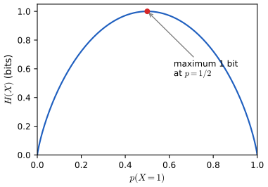
For a variable with \(K\) states, (a) \(0\le\Hent(X)\le\log K\); (b) \(\Hent(X)=0\) iff \(p\) is a delta distribution; (c) \(\Hent(X)=\log K\) iff \(p\) is uniform. For \(K=2\) with \(\theta=p(X=1)\) the entropy is the binary entropy function
\[ \Hent(\theta)=-[\theta\log\theta+(1-\theta)\log(1-\theta)], \tag{6.4} \]which is symmetric about \(\theta=\tfrac12\), where it attains its maximum of 1 bit (Figure 6.1).
Proof
(a) Each term \(-p_k\log p_k\) is \(\ge0\) because \(0\le p_k\le1\), so \(\Hent\ge0\), with equality iff every \(p_k\in\{0,1\}\), that is, iff exactly one \(p_k\) equals 1: (b). The upper bound is the non-negativity of the KL divergence from the uniform distribution \(u_k=1/K\): \[ 0\le\Dkl(p\|u)=\sum_kp_k\log(p_kK)=\log K-\Hent(p) \] (6.39), with equality iff \(p=u\) (Result 6.2); this is (c). Directly, \(\Hent(u)=-\sum_k\frac1K\log\frac1K=\log K\) (6.2). For \(K=2\), \(\Hent(\theta)=\Hent(1-\theta)\) by symmetry of (6.4), and the maximum is at \(\theta=\tfrac12\) by (c), where \(\Hent=\log2=1\) bit. ∎
6.1.1.1 Application: DNA sequence logos
pp. 208–209, (6.5), (6.6) Align \(N\) related DNA sequences and, at each position \(t\), count how often each letter occurs: \(N_{tk}=\sum_i\ind(X_{it}=k)\) for \(k\in\{A,C,G,T\}\), giving the column distribution \(\hat\theta_{tk}=N_{tk}/N\) (6.5), (6.6). The matrix of the \(\hat\theta_t\) is the position weight matrix (or sequence motif). In a sequence logo the stack at position \(t\) has total height \(R_t=2-\Hent(\hat\theta_t)\) bits, where \(2=\log_24\) is the largest possible entropy; the letters share that height in proportion to \(\hat\theta_{tk}\). A column that is the same letter everywhere has entropy 0 and height 2 (fully informative, typically conserved by evolution); a column with all four letters equally frequent has height 0.
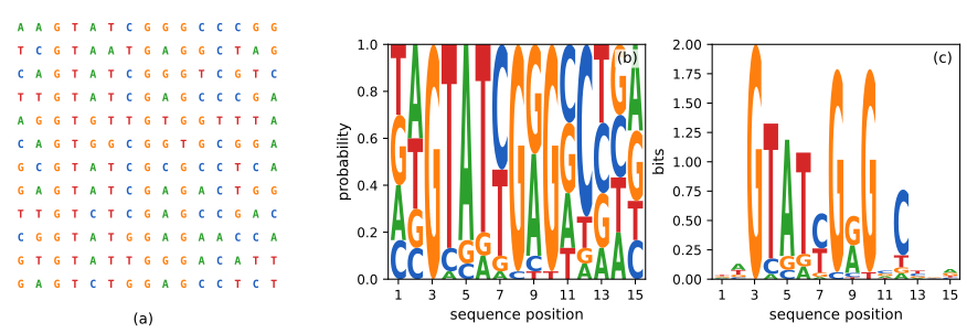
With only \(N=30\) sequences the empirical entropies are noisy: the plug-in estimate of an entropy is biased downwards (the estimated distribution is more concentrated than the truth on average), which makes columns look more conserved than they are. The next subsection says why and how large the effect is.
6.1.1.2 Estimating entropy
p. 209 Estimating \(\Hent\) means estimating \(p\), which needs many samples when there are many states (think of the distribution of words in English, with its long tail of rare words). The plug-in estimator \(\hat{\Hent}=\Hent(\hat p)\), with \(\hat p_k=n_k/N\), satisfies \(\E\hat{\Hent}\le\Hent(p)\) because \(\Hent\) is concave and \(\E\hat p=p\) (Jensen). To first order the bias is \(-(K-1)/(2N)\) nats, the correction of Miller (1955); for sharper remedies see Valiant and Valiant (2013), the paper the book cites. A numerical experiment at \(K=6\), \(N=40\) agrees with the first-order formula to within about 5 per cent (a bias of \(-0.0651\) nats against \(-0.0625\)).
6.1.2 Cross entropy
Definition 6.2 (cross entropy) p. 209, (6.7)
The cross entropy between distributions \(p\) and \(q\) on \(K\) states is
\[ \Hce(p,q)\triangleq-\sum_{k=1}^Kp_k\log q_k. \tag{6.7} \]It equals \(+\infty\) if \(q_k=0\) for some \(k\) with \(p_k>0\), and \(\Hce(p,p)=\Hent(p)\).
The book says that the cross entropy is the expected number of bits needed to compress samples from \(p\) using a code designed for \(q\), minimal at \(q=p\) (Shannon's source coding theorem). The statement needs two qualifications (integer code lengths, and what "designed for \(q\)" means), which are spelled out in the following box.
Filling the gap 6.1: the coding interpretation of entropy and cross entropy (Kraft's inequality and Shannon codes) pp. 207, 209, 214
Derivation
Setting. A prefix code assigns to state \(k\) a binary string of length \(l_k\in\{1,2,\dots\}\), no string being a prefix of another, so that a sequence of symbols can be decoded without separators. The expected length of the code under \(p\) is \(L=\sum_kp_kl_k\).
Kraft's inequality. The lengths of a prefix code satisfy \(\sum_k2^{-l_k}\le1\), and conversely any lengths with \(\sum_k2^{-l_k}\le1\) are the lengths of some prefix code. Proof. Let \(l_{\max}=\max_kl_k\) and picture the binary tree of depth \(l_{\max}\). A codeword of length \(l_k\) is a node at depth \(l_k\); its \(2^{l_{\max}-l_k}\) descendants at depth \(l_{\max}\) are disjoint from those of any other codeword (otherwise one codeword would be a prefix of the other). The total number of nodes at depth \(l_{\max}\) is \(2^{l_{\max}}\), so \(\sum_k2^{l_{\max}-l_k}\le2^{l_{\max}}\): the inequality. Conversely, order the lengths \(l_1\le\dots\le l_K\) and give state \(k\) the first \(l_k\) binary digits of \(\sum_{j\lt k}2^{-l_j}\); these strings are not prefixes of one another because \(\sum_{j\lt k}2^{-l_j}+2^{-l_k}\le1\) keeps the intervals \([\sum_{j\lt k}2^{-l_j},\sum_{j\le k}2^{-l_j})\) disjoint. \(\square\)
Entropy is a lower bound. Let \(c=\sum_k2^{-l_k}\le1\) and \(r_k=2^{-l_k}/c\), a distribution. Then \(l_k=-\log r_k-\log c\), so
\[ L=\sum_kp_kl_k=\Hce(p,r)+\log\tfrac1c=\Hent(p)+\Dkl(p\|r)+\log\tfrac1c\ \ge\ \Hent(p), \]because \(\Dkl\ge0\) (Result 6.2) and \(c\le1\). Equality needs \(r=p\) and \(c=1\), that is \(l_k=-\log p_k\) exactly, which is possible only if every \(p_k\) is a power of \(\tfrac12\).
A code designed for \(q\). Take the Shannon code lengths \(l_k=\lceil-\log q_k\rceil\). They satisfy Kraft, since \(\sum2^{-l_k}\le\sum q_k=1\). Because \(-\log q_k\le l_k\lt-\log q_k+1\), the expected length when the data really come from \(p\) obeys
\[ \Hce(p,q)\ \le\ L\ \lt\ \Hce(p,q)+1 . \]So, up to the integer-rounding of at most one bit per symbol (which disappears when long blocks of symbols are coded together), the cross entropy \(\Hce(p,q)\) is the cost per symbol of coding data from \(p\) with the code that is ideal for \(q\). Taking \(q=p\) gives \(\Hent(p)\le L\lt\Hent(p)+1\) (Shannon's source coding theorem for symbol codes), and the penalty for using \(q\) is \(\Hce(p,q)-\Hent(p)=\Dkl(p\|q)\) bits per symbol, the interpretation in Section 6.2.2. When \(q_k=0\) but \(p_k>0\) no finite code length is available: the cost is infinite. ∎
6.1.3 Joint entropy
pp. 209–210, (6.8)–(6.10) The joint entropy of two variables is the entropy of the pair,
\[ \Hent(X,Y)=-\sum_{x,y}p(x,y)\log_2p(x,y). \tag{6.8} \]Example: choose an integer \(n\) uniformly from \(\{1,\dots,8\}\), let \(X=1\) if \(n\) is even and \(Y=1\) if \(n\) is prime. The joint distribution has \(p(0,0)=p(1,1)=\tfrac18\) and \(p(0,1)=p(1,0)=\tfrac38\), and both marginals are uniform. Then
\[ \Hent(X,Y)=-\big(\tfrac18\log\tfrac18+\tfrac38\log\tfrac38+\tfrac38\log\tfrac38+\tfrac18\log\tfrac18\big)=1.81\text{ bits}, \tag{6.9} \]which is less than \(\Hent(X)+\Hent(Y)=2\) bits. The book states the general facts: \(\Hent(X,Y)\le\Hent(X)+\Hent(Y)\) with equality iff \(X\) and \(Y\) are independent, and
\[ \Hent(X,Y)\ \ge\ \max\{\Hent(X),\Hent(Y)\}\ \ge\ 0. \tag{6.10} \]Joint entropy extends to \(n\) variables in the obvious way. Use the joint entropy demo to reproduce 1.81 bits (preset 1) and to compare with a table of independent variables (preset 2).
6.1.4 Conditional entropy
Definition 6.3 (conditional entropy) pp. 210–211, (6.11)–(6.18)
The conditional entropy of \(Y\) given \(X\) is the average, over \(x\), of the entropy of the conditional distribution:
\[ \Hent(Y\given X)\triangleq\E_{p(X)}\big[\Hent(p(Y\given X))\big]=-\sum_{x,y}p(x,y)\log p(y\given x)=\Hent(X,Y)-\Hent(X). \tag{6.11--6.15} \]It satisfies \(\Hent(Y\given X)\le\Hent(Y)\) (6.16), with equality iff \(X\) and \(Y\) are independent, and the chain rule
\[ \Hent(X_1,\dots,X_n)=\sum_{i=1}^n\Hent(X_i\given X_1,\dots,X_{i-1}). \tag{6.18} \]If \(Y\) is a function of \(X\), then \(\Hent(Y\given X)=0\). The inequality (6.16) holds "on average": for a particular observation \(x\) the entropy of \(Y\) can go up, \(\Hent(Y\given X=x)\gt\Hent(Y)\) (see Exercise 6.3, where observing \(y=3\) raises the entropy of \(X\) from 1.75 to 2 bits).
Filling the gap 6.2: the chain rule, the two bounds on joint entropy, and when they are tight pp. 210–211, (6.10), (6.15)–(6.18)
Derivation
Chain rule (6.15), (6.17). Write \(p(x,y)=p(x)p(y\given x)\), so \(\log p(x,y)=\log p(x)+\log p(y\given x)\). Taking \(-\E_{p(x,y)}\) of both sides gives \[ \Hent(X,Y)=-\sum_xp(x)\log p(x)+\Hent(Y\given X) \], because \(\sum_yp(x,y)=p(x)\). For \(n\) variables use \[ p(x_1,\dots,x_n)=\prod_ip(x_i\given x_1,\dots,x_{i-1}) \] and the same argument (or induction on (6.17) applied to \((X_1,\dots,X_{n-1})\) and \(X_n\)), which is (6.18).
Upper bound. By (6.15), \(\Hent(Y\given X)\le\Hent(Y)\) is the same as \(\Hent(X,Y)\le\Hent(X)+\Hent(Y)\), which is the same as \(\Imut(X;Y)\ge0\) with \(\Imut(X;Y)=\Hent(X)+\Hent(Y)-\Hent(X,Y)\) (6.51). Now \[ \Hent(X)+\Hent(Y)-\Hent(X,Y)=\sum_{x,y}p(x,y)\log\frac{p(x,y)}{p(x)p(y)}=\Dkl(p(x,y)\|p(x)p(y))\ge0 \] by Result 6.2, with equality iff \(p(x,y)=p(x)p(y)\) for all \((x,y)\): independence. (The proof of Result 6.2 uses no property of \(\Imut\); there is no circularity.)
Lower bound (6.10). \[ \Hent(Y\given X)=\sum_xp(x)\Hent(p(Y\given X=x))\ge0 \], as an average of non-negative numbers, so \[ \Hent(X,Y)=\Hent(X)+\Hent(Y\given X)\ge\Hent(X) \]; by symmetry also \(\ge\Hent(Y)\). Equality \(\Hent(X,Y)=\Hent(X)\) holds iff \(\Hent(Y\given X=x)=0\) for every \(x\) with \(p(x)\gt0\), iff each conditional distribution \(p(\cdot\given x)\) is a delta: \(Y\) is a function of \(X\) (with probability 1).
"On average" only. Exercise 6.3(c)–(d) is a worked counterexample for individual values: \(\Hent(X\given Y=3)=2\gt\Hent(X)=\tfrac74\), yet \(\Hent(X\given Y)=\tfrac{11}8\lt\tfrac74\). ∎
6.1.5 Perplexity
pp. 211–212, (6.19)–(6.23) The perplexity of a distribution \(p\) is
\[ \operatorname{perplexity}(p)\triangleq2^{\Hent(p)}, \tag{6.19} \]the number of equally likely outcomes that would have the same entropy: a uniform distribution on \(K\) states has perplexity \(K\), and the smallest possible value is \(2^0=1\) (perfect prediction). For data \(\mathcal D\) with empirical distribution \(p_{\mathcal D}=\frac1N\sum_n\delta_{x_n}\) (6.20) and a model \(p\), the perplexity of the model is
\[ \operatorname{perplexity}(p_{\mathcal D},p)=2^{\Hce(p_{\mathcal D},p)},\qquad \Hce(p_{\mathcal D},p)=-\frac1N\sum_{n=1}^N\log p(x_n), \tag{6.21--6.22} \] \[ \operatorname{perplexity}(p_{\mathcal D},p)=2^{-\frac1N\log\prod_np(x_n)}=\Big(\prod_{n=1}^N\frac1{p(x_n)}\Big)^{1/N}. \tag{6.23} \]This is the geometric mean of the inverse predicted probabilities (the "exponentiated cross entropy"), used to evaluate language models. For a model that predicts each word uniformly among \(K\) possibilities whatever the context, the perplexity is \(K\) (the "branching factor"). Since \(\Hce(p^*,p)\ge\Hent(p^*)\), no model can have perplexity below \(2^{\Hent(p^*)}\), the perplexity of the true source \(p^*\).
Note that (6.19) is stated with base-2 logarithms; with natural logarithms the perplexity is \(e^{H}\), the same number. The entropy and KL demo shows both \(2^{\Hent(p)}\) and \(2^{\Hce(p,q)}\).
6.1.6 Differential entropy for continuous random variables *
Definition 6.4 (differential entropy) pp. 212–213, (6.24)–(6.28)
For a continuous variable \(X\) with density \(p\),
\[ h(X)\triangleq-\int p(x)\log p(x)\,\d x, \tag{6.24} \]when the integral exists. Examples: \(X\sim U(0,a)\) has \(h(X)=\log a\) (6.25); a Gaussian has
\[ h(\N(\bm\mu,\bm\Sigma))=\tfrac12\ln|2\pi e\bm\Sigma|=\tfrac12\ln\big[(2\pi e)^d|\bm\Sigma|\big]=\tfrac d2+\tfrac d2\ln(2\pi)+\tfrac12\ln|\bm\Sigma|, \tag{6.26} \] \[ h(\N(\mu,\sigma^2))=\tfrac12\ln(2\pi e\sigma^2). \tag{6.27} \]Unlike the discrete entropy, \(h\) can be negative: a density may exceed 1. For \(X\sim U(0,\tfrac18)\), \(h(X)=\log_2\tfrac18=-3\) bits. A way to read the number: describing a real variable to \(n\) bits of accuracy needs about \(h(X)+n\) bits, so \(U(0,\tfrac18)\), whose first three binary digits are zero, needs only \(n-3\).
6.1.6.2 Connection with variance
p. 213 The Gaussian entropy (6.27) increases with the variance, but in general entropy and variance are different things. Take an equal mixture of two unit-variance Gaussians centred at \(\pm\mu\): as \(\mu\) goes from 1 to 10 the variance increases from 2 to 101, whereas the entropy only increases to \(h(\N(0,1))+\ln2\) (the extra \(\ln2\) is the uncertainty about which component the sample came from). Numerically \(h=1.4189+0.6931=2.1121\) nats at \(\mu=10\), against 1.7558 at \(\mu=1\). The proof is in Filling the gap 6.3.
6.1.6.3 Discretisation
p. 213, (6.28) A simple way to estimate \(h(X)\) or the mutual information is to bin the data and use the empirical probabilities of the bins. Scott's rule for the number of bins is
\[ B=N^{1/3}\,\frac{\max(\mathcal D)-\min(\mathcal D)}{3.5\,\sigma(\mathcal D)}, \tag{6.28} \]where \(\sigma(\mathcal D)\) is the empirical standard deviation (this is the bin width \(3.5\sigma N^{-1/3}\) that minimises the integrated squared error of a histogram for Gaussian data, Scott, 1979). Binning does not scale to many dimensions, because the number of cells is \(B^d\). The behaviour of the binned estimator, including its bias, is explored in the binned mutual information demo and analysed in Filling the gap 6.8.
Filling the gap 6.3: differential entropy of a Gaussian, change of variables, quantisation, and the mixture claim pp. 212–213, (6.25)–(6.27)
Derivation
The Gaussian (6.26). With \[ \ln\N(\mathbf{x}\given\bm\mu,\bm\Sigma)=-\tfrac12\big[d\ln(2\pi)+\ln|\bm\Sigma|+(\mathbf{x}-\bm\mu)^\T\bm\Sigma^{-1}(\mathbf{x}-\bm\mu)\big] \] and \[ \E[(\mathbf{x}-\bm\mu)^\T\bm\Sigma^{-1}(\mathbf{x}-\bm\mu)]=\E\Tr[\bm\Sigma^{-1}(\mathbf{x}-\bm\mu)(\mathbf{x}-\bm\mu)^\T]=\Tr[\bm\Sigma^{-1}\bm\Sigma]=d \],
\[ h=-\E\ln\N=\tfrac12\big[d\ln(2\pi)+\ln|\bm\Sigma|+d\big]=\tfrac12\ln\big[(2\pi e)^d|\bm\Sigma|\big], \]which is (6.26); \(d=1\) gives (6.27) (in nats; divide by \(\ln2\) for bits).
The uniform (6.25). \(p=1/a\) on \((0,a)\): \(h=-\int_0^a\frac1a\log\frac1a\,\d x=\log a\).
Change of variables. If \(Y=aX\) with \(a\ne0\), then \(p_Y(y)=p_X(y/a)/|a|\) and \[ h(Y)=-\E\log p_Y(Y)=-\E\log p_X(X)+\log|a|=h(X)+\log|a| \]. More generally \(h(\mathbf{A}X)=h(X)+\log|\det\mathbf{A}|\). So differential entropy depends on the units of the variable (unlike the discrete entropy, and unlike the mutual information, which is invariant under invertible changes of variables).
Quantisation. Let \(X\) have a Riemann-integrable density \(p\) with finite \(h\) and finite entropy of the unit-cell quantisation, and let \(X^\Delta\) be \(X\) rounded to the grid of cells \([i\Delta,(i+1)\Delta)\), with \[ P(X^\Delta=i)=p_i=\int_{i\Delta}^{(i+1)\Delta}p \]. By the mean value theorem \(p_i=p(x_i)\Delta\) for some \(x_i\) in the cell. Then
\[ \Hent(X^\Delta)=-\sum_ip(x_i)\Delta\log p(x_i)-\log\Delta\ \longrightarrow\ h(X)-\log\Delta\qquad(\Delta\to0), \]since the sum is a Riemann sum of \(-p\log p\). For \(\Delta=2^{-n}\) this is \(\Hent(X^\Delta)\approx h(X)+n\) bits, the statement on p. 212 (Cover and Thomas, 2006, Theorem 8.3.1). Numerically, for \(X\sim\N(0,1)\), \(h=2.0471\) bits, and the entropy of the \(n\)-bit quantisation is 6.0471, 8.0471 and 10.0471 bits for \(n=4,6,8\), matching to \(10^{-3}\).
Mixture (Section 6.1.6.2). Let \(Z\in\{1,2\}\) with probabilities \(w_1,w_2\) pick a component, and \(X\given Z=j\sim p_j\), so that \(X\) has the mixture density \(p=\sum_jw_jp_j\). (i) Concavity of \(-t\log t\) gives \(h(X)\ge\sum_jw_jh(p_j)\). (ii) The pair \((X,Z)\) has \(h(X,Z)=\Hent(Z)+\sum_jw_jh(p_j)\) by the chain rule, and \(h(X,Z)=h(X)+\Hent(Z\given X)\ge h(X)\) because the discrete \(\Hent(Z\given X)\ge0\). Hence
\[ \sum_jw_jh(p_j)\ \le\ h(X)\ \le\ \sum_jw_jh(p_j)+\Hent(w). \]For two equal-variance Gaussian components, \(\sum_jw_jh(p_j)=\tfrac12\ln(2\pi e\sigma^2)\) whatever the separation, and \(\Hent(w)\le\ln2\). The variance of the mixture is \(\sigma^2+4w_1w_2\mu^2\to\infty\), while \(h\) stays in an interval of length at most \(\ln2\). When the components are far apart the posterior of \(Z\) given \(X\) is almost deterministic, \(\Hent(Z\given X)\to0\), and the upper bound is attained: \(h\to\tfrac12\ln(2\pi e\sigma^2)+\ln2\). ∎
6.2 Relative entropy (KL divergence) *
p. 213 To say how far a distribution \(q\) is from a target \(p\) we use a divergence \(D(p,q)\): a function with \(D(p,q)\ge0\) and equality iff \(p=q\). A metric would in addition be symmetric and satisfy the triangle inequality; the divergence discussed here has neither property (Result 6.2(c)). It is the Kullback–Leibler (KL) divergence, also called information gain or relative entropy (Kullback and Leibler, 1951).
See also (companion course): Result 1.22, Gibbs' inequality, and the consistency proof for maximum likelihood through the KL divergence in All of Statistics, Section 9.5.
6.2.1 Definition
Definition 6.5 (KL divergence) p. 213, (6.29), (6.30)
For discrete distributions and for densities respectively,
\[ \Dkl(p\|q)\triangleq\sum_{k=1}^Kp_k\log\frac{p_k}{q_k},\qquad \Dkl(p\|q)\triangleq\int p(x)\log\frac{p(x)}{q(x)}\,\d x. \tag{6.29, 6.30} \]Terms with \(p_k=0\) contribute 0; if \(q_k=0\) for some \(k\) with \(p_k\gt0\) then \(\Dkl(p\|q)=+\infty\).
6.2.2 Interpretation
p. 214, (6.31) Splitting the logarithm,
\[ \Dkl(p\|q)=\underbrace{\sum_kp_k\log p_k}_{-\Hent(p)}\ \underbrace{-\sum_kp_k\log q_k}_{\Hce(p,q)}=\Hce(p,q)-\Hent(p). \tag{6.31} \]By Filling the gap 6.1, \(\Hce(p,q)\) is (up to integer rounding) the average code length per symbol when data from \(p\) are compressed with a code built for \(q\), and \(\Hent(p)\) is the best achievable, so the KL divergence is the extra number of bits paid for the wrong model. It has further interpretations (as the expected log-likelihood ratio, as a gain in information when updating from \(q\) to \(p\)); the sequel to the book discusses them.
6.2.3 Example: KL divergence between two Gaussians
Result 6.3 (KL divergence between Gaussians) p. 214, (6.32), (6.33)
For \(D\)-dimensional Gaussians,
\[ \Dkl\big(\N(\mathbf{x}\given\bm\mu_1,\bm\Sigma_1)\,\|\,\N(\mathbf{x}\given\bm\mu_2,\bm\Sigma_2)\big)=\tfrac12\Big[\Tr(\bm\Sigma_2^{-1}\bm\Sigma_1)+(\bm\mu_2-\bm\mu_1)^\T\bm\Sigma_2^{-1}(\bm\mu_2-\bm\mu_1)-D+\ln\frac{\det\bm\Sigma_2}{\det\bm\Sigma_1}\Big], \tag{6.32} \]in nats. In one dimension,
\[ \Dkl\big(\N(\mu_1,\sigma_1^2)\,\|\,\N(\mu_2,\sigma_2^2)\big)=\ln\frac{\sigma_2}{\sigma_1}+\frac{\sigma_1^2+(\mu_1-\mu_2)^2}{2\sigma_2^2}-\frac12. \tag{6.33} \]Filling the gap 6.4: derivation of (6.32) and (6.33) p. 214
Derivation
Write \[ \Dkl(p_1\|p_2)=\E_1[\ln p_1(\mathbf{x})]-\E_1[\ln p_2(\mathbf{x})] \], with \(\E_1\) the expectation under \(\N(\bm\mu_1,\bm\Sigma_1)\). From \[ \ln\N(\mathbf{x}\given\bm\mu,\bm\Sigma)=-\tfrac12\big[D\ln2\pi+\ln|\bm\Sigma|+(\mathbf{x}-\bm\mu)^\T\bm\Sigma^{-1}(\mathbf{x}-\bm\mu)\big] \], and \[ \E_1[(\mathbf{x}-\bm\mu_1)^\T\bm\Sigma_1^{-1}(\mathbf{x}-\bm\mu_1)]=D \] (Filling the gap 6.3),
\[ \E_1[\ln p_1]=-\tfrac12\big[D\ln2\pi+\ln|\bm\Sigma_1|+D\big]. \]For the second term write \[ \mathbf{x}-\bm\mu_2=(\mathbf{x}-\bm\mu_1)+(\bm\mu_1-\bm\mu_2) \] and expand; the cross term has expectation zero because \(\E_1[\mathbf{x}-\bm\mu_1]=\mathbf{0}\), so
\[ \E_1\big[(\mathbf{x}-\bm\mu_2)^\T\bm\Sigma_2^{-1}(\mathbf{x}-\bm\mu_2)\big]=\Tr(\bm\Sigma_2^{-1}\bm\Sigma_1)+(\bm\mu_1-\bm\mu_2)^\T\bm\Sigma_2^{-1}(\bm\mu_1-\bm\mu_2), \]using \[ \E[\mathbf{z}^\T\mathbf{A}\mathbf{z}]=\Tr(\mathbf{A}\,\E[\mathbf{z}\mathbf{z}^\T]) \]. Hence \[ \E_1[\ln p_2]=-\tfrac12\big[D\ln2\pi+\ln|\bm\Sigma_2|+\Tr(\bm\Sigma_2^{-1}\bm\Sigma_1)+(\bm\mu_1-\bm\mu_2)^\T\bm\Sigma_2^{-1}(\bm\mu_1-\bm\mu_2)\big] \]. Subtracting, the \(D\ln2\pi\) terms cancel and
\[ \Dkl=\tfrac12\Big[\ln\frac{|\bm\Sigma_2|}{|\bm\Sigma_1|}-D+\Tr(\bm\Sigma_2^{-1}\bm\Sigma_1)+(\bm\mu_1-\bm\mu_2)^\T\bm\Sigma_2^{-1}(\bm\mu_1-\bm\mu_2)\Big], \]which is (6.32) (the quadratic form is symmetric in \(\bm\mu_1,\bm\mu_2\)). For \(D=1\), \(\bm\Sigma_i=\sigma_i^2\): \[ \tfrac12\ln\frac{\sigma_2^2}{\sigma_1^2}=\ln\frac{\sigma_2}{\sigma_1} \], \(\tfrac12\frac{\sigma_1^2}{\sigma_2^2}\) and \(\tfrac12\frac{(\mu_1-\mu_2)^2}{\sigma_2^2}\), giving (6.33). Two quick checks: the value is 0 when the two Gaussians coincide, and a numerical integration of (6.30) for \(\N(0.4,0.7^2)\) and \(\N(-0.9,1.9^2)\) agrees with (6.33) to \(10^{-8}\); in two dimensions a Monte Carlo average of \(\ln p_1-\ln p_2\) agrees with (6.32) to \(10^{-2}\). ∎
6.2.4 Non-negativity of KL
pp. 214–215, (6.34)–(6.39) The proof uses Jensen's inequality: if \(f\) is convex, \(\lambda_i\ge0\) and \(\sum_i\lambda_i=1\), then
\[ f\Big(\sum_{i=1}^n\lambda_ix_i\Big)\le\sum_{i=1}^n\lambda_if(x_i), \tag{6.34} \]"\(f\) of the average is at most the average of the \(f\)'s". For the concave \(\log\) the direction reverses: \(\log\E_x g(x)\ge\E_x\log g(x)\) (6.35).
Result 6.2 (the information inequality, Theorem 6.2.1, and its corollaries) p. 215, (6.36)–(6.39)
(a) \(\Dkl(p\|q)\ge0\), with equality iff \(p=q\). (b) \(\Hent(X)\le\log|\mathcal X|\), with equality iff \(p\) is uniform (Corollary 6.2.1). (c) \(\Dkl\) is not symmetric and does not satisfy the triangle inequality: for \(p=(0.9,0.1)\), \(q=(0.5,0.5)\), \(r=(0.1,0.9)\) in bits, \(\Dkl(p\|q)=0.531\), \(\Dkl(q\|p)=0.737\), but
\[ \Dkl(p\|r)=2.536\ \gt\ \Dkl(p\|q)+\Dkl(q\|r)=1.268. \]Filling the gap 6.5: Jensen's inequality by induction, two proofs of Theorem 6.2.1, the continuous case pp. 214–215
Derivation
Jensen by induction. Let \(f\) be convex on an interval. The case \(n=2\) is the definition of convexity. Suppose it holds for \(n\) points and take weights \(\lambda_1,\dots,\lambda_{n+1}\) with \(\lambda_{n+1}\lt1\) (if \(\lambda_{n+1}=1\) the claim is trivial). Put \(\mu_i=\lambda_i/(1-\lambda_{n+1})\) for \(i\le n\), so \(\sum_{i\le n}\mu_i=1\). Then
\[ f\Big(\sum_{i=1}^{n+1}\lambda_ix_i\Big)=f\Big(\lambda_{n+1}x_{n+1}+(1-\lambda_{n+1})\sum_{i\le n}\mu_ix_i\Big)\le\lambda_{n+1}f(x_{n+1})+(1-\lambda_{n+1})f\Big(\sum_{i\le n}\mu_ix_i\Big)\le\sum_{i=1}^{n+1}\lambda_if(x_i), \]using convexity for two points, then the induction hypothesis. If \(f\) is strictly convex, equality holds iff all \(x_i\) with \(\lambda_i\gt0\) are equal (strictness at the first step forces \(x_{n+1}=\sum_{i\le n}\mu_ix_i\), and at the second, by induction, the others equal each other; the common value is then the average). For a random variable, \(f(\E X)\le\E f(X)\) follows by the same argument or by a supporting line at \(\E X\) (see All of Statistics, Theorem 4.9). Apply it to the convex function \(-\ln\).
Proof 1 (the book's, with the equality case made explicit). Let \(A=\{x:p(x)\gt0\}\). Jensen with weights \(p(x)\) on \(A\) and the concave \(\ln\) gives
\[ -\Dkl(p\|q)=\sum_{x\in A}p(x)\ln\frac{q(x)}{p(x)}\le\ln\sum_{x\in A}p(x)\frac{q(x)}{p(x)}=\ln q(A)\le\ln1=0. \]Equality in the first step needs \(q(x)/p(x)\) to be constant, \(=c\), on \(A\) (strict concavity), and in the second \(q(A)=1\). Then \(c\,p(A)=c=q(A)=1\), so \(q=p\) on \(A\), and \(q=0\) off \(A\) because \(q(A)=1\): \(q=p\). (Here \(c\) is the ratio \(q/p\); the book writes \(p=cq\) and the argument is the same.) If \(q(x)=0\) for some \(x\in A\) the divergence is \(+\infty\), consistent with the claim.
Proof 2 (one line). The inequality \(\ln t\le t-1\) holds for \(t\gt0\), with equality iff \(t=1\) (the tangent to the concave \(\ln\) at 1 lies above it). With \(t=q/p\), \[ -\Dkl(p\|q)=\sum_Ap\ln\frac qp\le\sum_Ap(\frac qp-1)=q(A)-1\le0 \], and equality needs \(q=p\) on \(A\) and \(q(A)=1\).
Continuous distributions. If \(P\) has density \(p\) and \(Q\) has density \(q\) and \(p\) vanishes wherever \(q\) does (\(P\ll Q\)), the same proof with sums replaced by integrals gives \(\Dkl(p\|q)\ge0\), with equality iff \(p=q\) almost everywhere; otherwise \(\Dkl=\infty\). The discrete and continuous cases are one theorem about densities with respect to a common reference measure.
Corollary 6.2.1. With \(u(x)=1/|\mathcal X|\): \(0\le\Dkl(p\|u)=\log|\mathcal X|-\Hent(X)\) (6.39).
The counter-examples of Result 6.2(c). In bits: \[ \Dkl(p\|q)=0.9\log_21.8+0.1\log_20.2=0.7634-0.2322=0.531 \]; \[ \Dkl(q\|p)=0.5\log_2\frac{0.5}{0.9}+0.5\log_2\frac{0.5}{0.1}=-0.4240+1.1610=0.737 \]; \(\Dkl(q\|r)=0.737\) by symmetry of the pair \((q,r)\) with \((q,p)\); \[ \Dkl(p\|r)=0.9\log_29+0.1\log_2\frac19=0.8\log_29=2.536 \]. ∎
Cross-references in the book
In the proof of Fano's inequality (p. 225) the book says "conditioning reduces entropy (see Section 6.2.4)"; that fact is (6.16) in Section 6.1.4 (and again follows from \(\Imut\ge0\) in Section 6.3.2). Section 6.2.4 is the section on Jensen's inequality and the information inequality, which is what the fact depends on.
6.2.5 KL divergence and MLE
pp. 215–216, (6.40)–(6.44) Suppose we look for the \(q\) closest to \(p\) in KL, \[ q^*=\arg\min_q\Dkl(p\|q)=\arg\min_q\big[\int p\log p-\int p\log q\big] \] (6.40). Take \(p\) to be the empirical distribution \(p_{\mathcal D}(x)=\frac1N\sum_n\delta(x-x_n)\) (6.41). The sifting property of the delta function gives
\[ \Dkl(p_{\mathcal D}\|q)=-\frac1N\sum_{n=1}^N\log q(x_n)+C,\qquad C=\int p_{\mathcal D}\log p_{\mathcal D}, \tag{6.42--6.44} \]where \(C\) does not depend on \(q\). So minimising the KL divergence to the empirical distribution is the same as minimising the average negative log likelihood (the "cross entropy objective"): maximum likelihood is KL minimisation. (For continuous data \(C=-\infty\) because \(p_{\mathcal D}\) is a sum of deltas; the equivalence is between the minimisers, and it is cleanest to read the identity for a discrete \(x\), where \(C=-\Hent(p_{\mathcal D})\) is finite.) For a categorical model this gives the empirical frequencies: minimising \[ \Hce(p_{\mathcal D},q)=\Hent(p_{\mathcal D})+\Dkl(p_{\mathcal D}\|q) \] over \(q\) is solved by \(q=p_{\mathcal D}\) by Result 6.2(a) (confirmed numerically with a generic optimiser). The same argument shows the consistency of maximum likelihood through the population version \(\Dkl(p^*\|q_\theta)\) (All of Statistics, Theorem 9.13).
The book points to the weakness of this view: the empirical distribution puts all its mass on the training points, so likelihood training puts too much weight on the training set, and techniques such as smoothing the empirical distribution (kernel density estimation) or data augmentation try to correct it.
6.2.6 Forward vs reverse KL
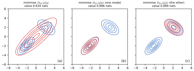
pp. 216–217, (6.45), (6.46) To approximate a distribution \(p\) by a simpler \(q\), one can minimise either divergence. The forward (inclusive) KL \(\Dkl(p\|q)=\int p\log\frac pq\) (6.45) is the M-projection (moment projection); it is infinite if \(q(x)=0\) where \(p(x)\gt0\), so \(q\) is pushed to cover all the mass of \(p\): zero avoiding, mode covering, typically over-estimating the support. The reverse (exclusive) KL \(\Dkl(q\|p)=\int q\log\frac qp\) (6.46) is the I-projection (information projection); it is infinite if \(q(x)\gt0\) where \(p(x)=0\), so \(q\) avoids regions where \(p\) is small: zero forcing, mode seeking, typically under-estimating the support. Figure 6.3 shows a unimodal Gaussian fitted to a bimodal \(p\).
Filling the gap 6.6: the forward KL projection matches moments; why reverse KL is mode seeking and has several minima pp. 216–217
Derivation
Forward KL onto Gaussians is moment matching. Let \(p\) have mean \(\mathbf{m}\) and covariance \(\mathbf{C}\) (finite). For \(q=\N(\bm\mu,\bm\Sigma)\),
\[ \Dkl(p\|q)=-h(p)+\tfrac12\ln|2\pi\bm\Sigma|+\tfrac12\E_p\big[(\mathbf{x}-\bm\mu)^\T\bm\Sigma^{-1}(\mathbf{x}-\bm\mu)\big], \]and \[ \E_p[(\mathbf{x}-\bm\mu)^\T\bm\Sigma^{-1}(\mathbf{x}-\bm\mu)]=\Tr(\bm\Sigma^{-1}\mathbf{C})+(\mathbf{m}-\bm\mu)^\T\bm\Sigma^{-1}(\mathbf{m}-\bm\mu) \]. The last term is \(\ge0\) and vanishes iff \(\bm\mu=\mathbf{m}\), whatever \(\bm\Sigma\). With \(\bm\mu=\mathbf{m}\) and \(\bm\Lambda=\bm\Sigma^{-1}\) we minimise \[ \tfrac12[-\ln|\bm\Lambda|+\Tr(\bm\Lambda\mathbf{C})] \] over positive definite \(\bm\Lambda\): this is convex (\(-\ln|\cdot|\) is convex), with gradient \(\tfrac12(-\bm\Lambda^{-1}+\mathbf{C})\), which vanishes at \(\bm\Sigma=\bm\Lambda^{-1}=\mathbf{C}\). So the minimiser is \(\N(\mathbf{m},\mathbf{C})\), the Gaussian with the same first two moments as \(p\) (Figure 6.3a). The same calculation for any exponential family \(q_\eta\propto\exp(\eta^\T T(x))\) shows that the forward KL is minimised when \(\E_{q}[T]=\E_p[T]\), hence the name "moment projection". For the mixture of the demonstration, \(p=w\N(-m,s^2)+(1-w)\N(m,s^2)\) has mean \((1-2w)m\) and variance \(s^2+4w(1-w)m^2\): for \(m=2.5\), \(s=1\), \(w=\tfrac12\) the fitted \(q\) is \(\N(0,2.69^2)\), a broad Gaussian that puts its mode where \(p\) has a valley.
Reverse KL is infinite off the support of \(p\). If \(q\) has mass where \(p=0\), \(\Dkl(q\|p)=\infty\); with \(p\) positive everywhere (as for a Gaussian mixture) the divergence is finite, but the integrand \(q\ln(q/p)\) is large where \(q\) is not small and \(p\) is, so \(q\) is penalised for placing mass in a valley of \(p\). This is the "zero forcing" behaviour.
Why two local minima. Take \(p=\tfrac12q_1+\tfrac12q_2\), with \(q_1=\N(-m,s^2)\), \(q_2=\N(m,s^2)\), and the candidate \(q=q_1\). Then
\[ \Dkl(q_1\|p)=\E_{q_1}\Big[\ln\frac{q_1}{\tfrac12q_1+\tfrac12q_2}\Big]=\ln2-\E_{q_1}\Big[\ln\Big(1+\frac{q_2}{q_1}\Big)\Big], \]and \(\E_{q_1}\ln(1+q_2/q_1)\gt0\) tends to 0 as \(m/s\to\infty\): the ratio is \(q_2/q_1=\exp(-2m^2/s^2+2mz/s)\) at \(x=-m+sz\), \(z\sim\N(0,1)\). So \(\Dkl(q_1\|p)\to\ln2\) from below as the modes separate, and the same holds for \(q_2\) by symmetry: there are two equally good fits, one per mode. They are local minima because moving \(q\) towards the valley between the modes increases the divergence (the demonstration shows the two dips of the reverse-KL profile), whereas the forward KL has the single moment-matching minimiser. In the demonstration (\(m=2.5\), \(s=1\), \(w=\tfrac12\)) the reverse minima have value 0.6665 nats at \(q\approx\N(\mp2.386,1.136^2)\) (slightly wider and nearer the centre than \(q_1\)); the forward optimum has \(\Dkl(p\|q)=0.3146\) nats, measured in its own direction. When the weights are unequal the minimum on the lighter component can disappear: for \(w=\tfrac14\) optimisers started at either mode end at the heavier one, with value 0.276, close to \(-\ln0.75=0.288\), the cost of the missing component. ∎
See also (companion course): Section 10.1.2, properties of factorised approximations, Result 10.6 (forward KL over factorised \(q\) gives the marginals; compare Exercise 6.4) and the Gaussian approximations demo.
6.3 Mutual information *
p. 217 How dependent are two random variables? One way to answer is to compare the true joint distribution with the one we would have if they were independent, and measure the gap with the KL divergence. This is the mutual information.
See also (companion course): Result 1.23, mutual information.
6.3.1 Definition
Definition 6.6 (mutual information) p. 217, (6.47), (6.48)
The mutual information between \(X\) and \(Y\) is the KL divergence between the joint distribution and the product of the marginals:
\[ \Imut(X;Y)\triangleq\Dkl\big(p(x,y)\,\|\,p(x)p(y)\big)=\sum_{y\in\mathcal Y}\sum_{x\in\mathcal X}p(x,y)\log\frac{p(x,y)}{p(x)p(y)}, \tag{6.47} \]with sums replaced by integrals for continuous variables. The notation \(\Imut(X;Y)\) with a semicolon allows \(X\) or \(Y\) to stand for several variables, e.g. \(\Imut(X;Y,Z)\). By Result 6.2,
\[ \Imut(X;Y)\ge0, \tag{6.48} \]with equality iff \(p(x,y)=p(x)p(y)\), that is, iff \(X\) and \(Y\) are independent. This holds for continuous variables too, since the proof does not use a sum.
6.3.2 Interpretation
p. 218, (6.49)–(6.51) As a KL divergence, \(\Imut\) is the information gained by moving from the model \(p(x)p(y)\) that treats the variables as independent to the true joint. In terms of entropies,
\[ \Imut(X;Y)=\Hent(X)-\Hent(X\given Y)=\Hent(Y)-\Hent(Y\given X), \tag{6.49} \] \[ \Imut(X;Y)=\Hent(X,Y)-\Hent(X\given Y)-\Hent(Y\given X), \tag{6.50} \] \[ \Imut(X;Y)=\Hent(X)+\Hent(Y)-\Hent(X,Y). \tag{6.51} \]So \(\Imut\) is the reduction in uncertainty about \(X\) after observing \(Y\), and symmetrically. It gives another proof that conditioning, on average, reduces entropy: \(0\le\Imut(X;Y)=\Hent(X)-\Hent(X\given Y)\). These identities are summarised by the information diagram of Figure 6.4 (a hand-drawn schematic, not reproduced here): \(\Hent(X)\) and \(\Hent(Y)\) are overlapping regions whose overlap is \(\Imut\), and \(\Hent(X,Y)\) is their union. The bars drawn by the joint entropy demo are the same picture with lengths in bits. (As a signed measure the diagram can be misleading for three or more variables, where the "triple overlap" can be negative; see the XOR example below.)
6.3.3 Example
p. 218, (6.52)–(6.55) In the even/prime example, normalising each row of the joint table gives \(p(Y\given X)\): \(p(Y=1\given X=0)=\tfrac34\), \(p(Y=1\given X=1)=\tfrac14\). Hence
\[ \Hent(Y\given X)=-\big(\tfrac18\log\tfrac14+\tfrac38\log\tfrac34+\tfrac38\log\tfrac34+\tfrac18\log\tfrac14\big)=0.81\text{ bits},\qquad \Imut(X;Y)=\Hent(Y)-\Hent(Y\given X)=0.19\text{ bits}, \tag{6.52, 6.53} \] \[ \Hent(X,Y)=\Hent(X\given Y)+\Imut(X;Y)+\Hent(Y\given X)=0.81+0.19+0.81=1.81\text{ bits}. \tag{6.54, 6.55} \]6.3.4 Conditional mutual information
Definition 6.7 (conditional mutual information and the chain rule) p. 219, (6.56)–(6.63)
\[ \Imut(X;Y\given Z)\triangleq\E_{p(z)}\big[\Imut(X;Y)\given Z=z\big]=\E_{p(x,y,z)}\Big[\log\frac{p(x,y\given z)}{p(x\given z)p(y\given z)}\Big], \tag{6.56, 6.57} \] \[ =\Hent(X\given Z)+\Hent(Y\given Z)-\Hent(X,Y\given Z)=\Hent(X\given Z)-\Hent(X\given Y,Z)=\Hent(Y\given Z)-\Hent(Y\given X,Z) \tag{6.58, 6.59} \] \[ =\Hent(X,Z)+\Hent(Y,Z)-\Hent(Z)-\Hent(X,Y,Z)=\Imut(Y;X,Z)-\Imut(Y;Z). \tag{6.60, 6.61} \]Rewriting (6.61) gives \(\Imut(Z,Y;X)=\Imut(Z;X)+\Imut(Y;X\given Z)\) (6.62), and for \(N\) variables the chain rule for mutual information
\[ \Imut(Z_1,\dots,Z_N;X)=\sum_{n=1}^N\Imut(Z_n;X\given Z_1,\dots,Z_{n-1}). \tag{6.63} \]The extra information that \(Y\) gives about \(X\) over and above what \(Z\) already does is \(\Imut(Y;X\given Z)\).
A notational slip in (6.56)
The book writes \[ \Imut(X;Y\given Z)\triangleq\E_{p(Z)}[\Imut(X;Y)\given Z] \], which reads as if \(\Imut(X;Y)\) were a random quantity conditioned on \(Z\). What is meant is the average over \(z\) of the mutual information of the conditional distribution \(p(x,y\given Z=z)\), which is (6.57); the values of (6.56) and (6.57) are the same, as checked numerically on a random three-way table.
Filling the gap 6.7: the identities (6.49)–(6.63) pp. 218–219
Derivation
(6.49). Use \(p(x,y)/(p(x)p(y))=p(x\given y)/p(x)\): \[ \Imut=\sum p(x,y)\log p(x\given y)-\sum_xp(x)\log p(x)=-\Hent(X\given Y)+\Hent(X) \], by (6.13). Exchanging \(X\) and \(Y\) gives the second form.
(6.51). Expanding the logarithm in (6.47), \[ \Imut=\sum p(x,y)\log p(x,y)-\sum_xp(x)\log p(x)-\sum_yp(y)\log p(y)=-\Hent(X,Y)+\Hent(X)+\Hent(Y) \].
(6.50). From the chain rule (6.15), \(\Hent(X\given Y)=\Hent(X,Y)-\Hent(Y)\) and \(\Hent(Y\given X)=\Hent(X,Y)-\Hent(X)\), so \[ \Hent(X,Y)-\Hent(X\given Y)-\Hent(Y\given X)=\Hent(X)+\Hent(Y)-\Hent(X,Y) \], which is (6.51).
Conditional MI. Fix \(z\) and apply (6.49), (6.51) to the conditional distribution \(p(x,y\given z)\); averaging over \(p(z)\) gives (6.58) and (6.59) with the conditional entropies \[ \Hent(\cdot\given Z)=\sum_zp(z)\Hent(\cdot\given Z=z) \]. By the chain rule \(\Hent(X,Y\given Z)=\Hent(X,Y,Z)-\Hent(Z)\), \(\Hent(X\given Z)=\Hent(X,Z)-\Hent(Z)\), so (6.58) becomes (6.60). For (6.61) write \[ \Imut(Y;X,Z)=\Hent(Y)+\Hent(X,Z)-\Hent(X,Y,Z) \] by (6.51) and \(\Imut(Y;Z)=\Hent(Y)+\Hent(Z)-\Hent(Y,Z)\); the difference is \(\Hent(X,Z)+\Hent(Y,Z)-\Hent(Z)-\Hent(X,Y,Z)\), which is (6.60).
(6.62) and (6.63). (6.61) with the roles of \(X\) and \(Y\) interchanged says \(\Imut(X;Y\given Z)=\Imut(X;Y,Z)-\Imut(X;Z)\), i.e. \(\Imut(X;Y,Z)=\Imut(X;Z)+\Imut(X;Y\given Z)\), and \(\Imut\) is symmetric: (6.62). For (6.63), induct on \(N\): apply (6.62) with \(Z=Z_1,\dots,Z_{N-1}\) and \(Y=Z_N\).
Non-negativity and an example where conditioning increases the information. \[ \Imut(X;Y\given Z)=\sum_zp(z)\Dkl(p(x,y\given z)\|p(x\given z)p(y\given z))\ge0 \]. But \(\Imut(X;Y\given Z)\) can be larger than \(\Imut(X;Y)\): let \(X,Y\) be independent fair bits and \(Z=X\oplus Y\) (exclusive or). Then \(\Imut(X;Y)=0\), while given \(Z\) the variable \(Y\) is determined by \(X\): \(\Imut(X;Y\given Z)=\Hent(X\given Z)=1\) bit. By (6.62), \(\Imut(X;Y,Z)=0+1=1\) bit although neither \(Y\) nor \(Z\) alone tells anything about \(X\). (In the information diagram of three variables the central region is therefore \(-1\) here.) All identities were also confirmed numerically on random three-way tables. ∎
6.3.5 MI as a "generalized correlation coefficient"
Result 6.4 (mutual information of a bivariate Gaussian) p. 220, (6.64)–(6.70)
If \[ (X,Y)\sim\N\big(\mathbf{0},\begin{pmatrix}\sigma^2&\rho\sigma^2\\\rho\sigma^2&\sigma^2\end{pmatrix}\big) \] (6.64), then \[ h(X,Y)=\tfrac12\log[(2\pi e)^2\sigma^4(1-\rho^2)] \] (6.65), \(h(X)=h(Y)=\tfrac12\log(2\pi e\sigma^2)\) (6.66), and
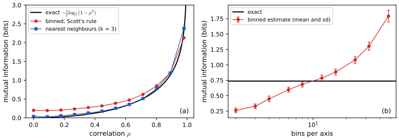
\[ \Imut(X;Y)=h(X)+h(Y)-h(X,Y)=-\tfrac12\log(1-\rho^2). \tag{6.67--6.70} \]It is 0 for \(\rho=0\) (independence) and tends to \(\infty\) as \(\rho\to\pm1\), where \(Y=\pm X\) and \(Y\) tells \(X\) exactly.
The mutual information of a Gaussian pair is thus a monotone function of \(|\rho|\) alone, which is why \(\Imut\) is called a generalised correlation coefficient: for non-Gaussian pairs it still measures dependence, but it can see non-linear relations that \(\rho\) misses. To estimate it from samples of two scalars one can bin both variables (the plug-in estimate described next), use the nearest-neighbour estimator of Kraskov, Stögbauer and Grassberger (2004) (the KSG estimator, in sklearn.feature_selection.mutual_info_regression), or a more recent estimator (Gao et al., 2018; Holmes and Nemenman, 2019, the papers the book cites).
Filling the gap 6.8: the Gaussian case, invariance, and the bias of the binned estimator pp. 220, 213
Derivation
(6.65)–(6.70). The covariance matrix \(\bm\Sigma\) in (6.64) has \[ \det\bm\Sigma=\sigma^4-\rho^2\sigma^4=\sigma^4(1-\rho^2) \] (positive iff \(|\rho|\lt1\)). By (6.26) with \(d=2\), \[ h(X,Y)=\tfrac12\log[(2\pi e)^2\sigma^4(1-\rho^2)] \]; by (6.27) the marginals are \(\N(0,\sigma^2)\) with \(h=\tfrac12\log(2\pi e\sigma^2)\). Then \[ h(X)+h(Y)-h(X,Y)=\log(2\pi e\sigma^2)-\tfrac12\log[(2\pi e\sigma^2)^2(1-\rho^2)]=-\tfrac12\log(1-\rho^2) \]: the factor \(2\pi e\sigma^2\) cancels, so the result does not depend on \(\sigma\). (For continuous variables the mutual information is the difference of differential entropies, (6.51) with \(h\), which is legitimate because \(\Imut=\Dkl(p(x,y)\|p(x)p(y))\) is an integral of the same logarithms as in (6.47).) Evaluating (6.26) in code reproduces (6.70) for \(\rho=0,0.5,0.9,-0.8\) to \(10^{-10}\).
Invariance. If \(X'=g(X)\) and \(Y'=k(Y)\) with \(g,k\) invertible and differentiable, the Jacobians cancel in the ratio \(p(x,y)/(p(x)p(y))\), so \(\Imut(X';Y')=\Imut(X;Y)\): unlike \(h\) (see Filling the gap 6.3), the mutual information does not depend on the scale or parametrisation of the variables. The correlation is invariant only under affine maps.
Bias of the binned (plug-in) estimator. Cut each variable into \(B\) cells and let \(n_{ij}\) count the points in cell \((i,j)\), \(N=\sum n_{ij}\), \(\hat p_{ij}=n_{ij}/N\) and \(\hat\imath=\Imut(\hat p)\) in nats. If \(X\) and \(Y\) are independent, the expected counts under independence are \(E_{ij}=n_{i\cdot}n_{\cdot j}/N\) and
\[ 2N\hat\imath=2\sum_{ij}n_{ij}\ln\frac{n_{ij}}{E_{ij}}=G, \]the likelihood-ratio ("G") statistic of the test of independence in a \(B\times B\) table. By the expansion of Exercise 6.2 (\(\ln(1+t)=t-t^2/2+\dots\) with \(t=(n_{ij}-E_{ij})/E_{ij}\) and \(\sum(n_{ij}-E_{ij})=0\)), \(G\approx\sum_{ij}(n_{ij}-E_{ij})^2/E_{ij}\), Pearson's statistic, and both converge in distribution to \(\chi^2_{(B-1)^2}\) when \(N\to\infty\) with \(B\) fixed (Pearson's theorem with the \(2(B-1)\) marginal parameters estimated). Therefore
\[ \E[\hat\imath]\approx\frac{(B-1)^2}{2N}\ \text{nats}\qquad(\text{independent variables, }N\gg B^2). \]In general the bias is of the same order, \((B_X-1)(B_Y-1)/(2N)\), so a table with many cells and few points reports dependence that is not there. In a simulation with \(N=2000\), \(B=8\) and independent Gaussians the average estimate is within 10 per cent of \((B-1)^2/(2N)=0.01225\) nats. The expansion fails when most cells are nearly empty: for \(N=100\) and \(B=20\) the formula would predict a bias of 1.8 nats, but the estimate cannot exceed the entropies of the two binned margins, and the demonstration shows 1.67 bits (1.16 nats) for independent data. A practical remedy is to compare the estimate with the same estimate after permuting one of the variables (the dashed curve in the demonstration), or to subtract the bias. Scott's rule (6.28) chooses a moderate \(B\) of order \(N^{1/3}\), so that \(B^2/N\to0\). ∎
6.3.6 Normalized mutual information
p. 221, (6.71)–(6.75) To get a measure of dependence between 0 and 1: since \[ \Imut(X;Y)=\Hent(X)-\Hent(X\given Y)\le\Hent(X) \] and likewise \(\le\Hent(Y)\) (6.71), (6.72),
\[ 0\le\Imut(X;Y)\le\min(\Hent(X),\Hent(Y)), \tag{6.73} \] \[ \operatorname{NMI}(X,Y)=\frac{\Imut(X;Y)}{\min(\Hent(X),\Hent(Y))}\le1. \tag{6.74} \]\(\operatorname{NMI}=0\) iff \(X,Y\) are independent. If \(\operatorname{NMI}=1\) and \(\Hent(X)\lt\Hent(Y)\), then \(\Hent(X\given Y)=0\) (6.75), so \(X\) is a function of \(Y\) (compare Result 6.1 and Gap 6.2). Example: \(X\) with pmf \((0.5,0.25,0.25)\) has \(\Hent(X)=1.5\) bits and \(\Imut(X;X)=\Hent(X)=1.5\), so \(\operatorname{NMI}(X,X)=1\). For continuous variables the normalisation by the differential entropy is awkward (it is not scale invariant and can be negative), so one normalises after quantising, which depends on the grid.
6.3.7 Maximal information coefficient
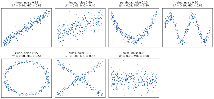
pp. 221–224, (6.76) The maximal information coefficient (MIC) of Reshef et al. (2011) searches over grids so as not to depend on a single binning:
\[ \operatorname{MIC}(X,Y)=\max_G\frac{\Imut\big((X,Y)|_G\big)}{\log\|G\|}, \tag{6.76} \]where \(G\) ranges over 2-d grids with \(G_x\) columns and \(G_y\) rows, \((X,Y)|_G\) is the discretisation of the data onto \(G\), and \(\|G\|=\min(G_x,G_y)\). The resolution is limited by \(G_xG_y\le B(n)=n^{\alpha}\), \(\alpha=0.6\) in the paper. For each grid shape \((k,l)\) one records the largest mutual information over all placements of the grid lines, divided by \(\log\min(k,l)\), to form the "characteristic matrix" \(M(k,l)\) (Figure 6.5, a schematic of the search, not reproduced); the MIC is its largest entry. The authors show that the statistic is equitable (it gives similar scores to equally noisy relationships of different forms). Reshef et al. (2016) give a faster estimator MICe, using one-dimensional optimisation with dynamic programming, and a second statistic TICe, the sum of the entries, which has more power to detect weak relationships and is suggested for screening. A value near 0 means no relationship and near 1 a noise-free relationship of any form, linear or not; for this reason the MIC has been called "a correlation for the 21st century". Figure 6.7 of the book applies it to 357 health indicators (63,546 pairs); that data set is not available here, and the figure is not reproduced.
The denominator in (6.76)
The book describes \(\log\|G\|\) as "the entropy of a uniform joint distribution". It is the largest value that the mutual information on a \(k\times l\) grid can take, \(\log\min(k,l)\): \[ \Imut\le\min(\Hent(X),\Hent(Y))\le\log\min(k,l) \], with equality when the cell variable with fewer values is uniform and determined by the other (Filling the gap 6.9). This is why each entry \(M(k,l)\le1\).
Filling the gap 6.9: why correlation misses a parabola; the range of NMI and MIC; the simplified MIC used here pp. 220–223
Derivation
Correlation is blind to even relationships. If \(X\) has a distribution symmetric about 0 (so \(\E X=\E X^3=0\)) and \(Y=X^2\), then \(\cov(X,Y)=\E X^3-\E X\,\E X^2=0\), so \(\rho=0\) although \(Y\) is a deterministic function of \(X\) and \(\Imut(X;Y)=\Hent(Y)\) (discrete case) is large. Figure 6.6 (parabola) and the demonstration (preset 2) show \(R^2\approx0.002\) with binned \(\Imut\approx1.1\) bits.
NMI and MIC are in \([0,1]\). \[ \Imut(X;Y)=\Hent(X)-\Hent(X\given Y)\le\Hent(X) \] because \(\Hent(X\given Y)\ge0\) (Gap 6.2); the same with \(Y\): (6.73). On a grid with \(k\) columns and \(l\) rows, \(\Hent(X|_G)\le\log k\) and \(\Hent(Y|_G)\le\log l\) (Result 6.1), so \(\Imut\big((X,Y)|_G\big)\le\log\min(k,l)\), which is the denominator in the definition of \(M(k,l)\) (Section 6.3.7): hence \(0\le M(k,l)\le1\) and \(\operatorname{MIC}\in[0,1]\). \(M(k,l)=1\) iff the grid cell variable with fewer values is uniform and a function of the other.
Invariance. The grid searches use the data only through ranks (equal-count rows) and the positions of cut points between ordered data values, so the MIC is unchanged by monotone increasing transformations of \(X\) or \(Y\) (confirmed numerically: \[ \operatorname{MIC}(e^{3X},Y)=\operatorname{MIC}(X,Y) \] for the sine example).
The search used in this course. The exact maximisation over all grids is expensive. The code (mic in ch06_information_theory.py) follows the idea of Reshef et al. (2011): for \(l\) rows it takes the equal-count partition of the \(y\)-axis and finds the best \(k\) column cuts of the \(x\)-axis by dynamic programming. The mutual information with fixed rows is \[ \Hent(\text{rows})-\Hent(\text{rows}\given\text{columns}) \], and \[ \Hent(\text{rows}\given\text{columns})=-\tfrac1N\sum_{\text{cols}}\sum_rn_{r,c}\ln(n_{r,c}/n_{\cdot c}) \] is a sum over columns, so the best split is found by \(f(c,j)=\max_i[f(c-1,i)+g(i,j)]\), where \(g(i,j)\) is the contribution of one column that spans candidate cut points \(i\) to \(j\). The cut points are restricted to at most 40 quantiles of the \(x\)-values, both axis orientations are tried, and the maximum is over \(kl\le n^{0.6}\). With these simplifications the values are lower bounds on the exact grid optimum and are not those of the published implementation, but the pattern (near 1 for a noiseless line, high for clear non-linear relations, near 0 for independence) is the same: a noiseless line gives 1.00, independent noise 0.08, the sine with noise 0.2 gives 0.86. The claim of equitability is an empirical property of the statistic, shown by simulation in the cited paper; it is not proved here. ∎
6.3.8 Data processing inequality
Result 6.5 (data processing inequality, Theorem 6.3.1) p. 223, (6.77)–(6.79)
If \(X\to Y\to Z\) is a Markov chain, that is \(X\perp Z\given Y\), then \(\Imut(X;Y)\ge\Imut(X;Z)\) and \(\Imut(Y;Z)\ge\Imut(X;Z)\). Equality in the first holds iff \(X\perp Y\given Z\).
Processing a noisy observation \(Y\) of an unknown \(X\) into \(Z=f(Y)\) (or any randomised function of \(Y\)) cannot increase the information about \(X\). The proof expands \(\Imut(X;Y,Z)\) with the chain rule (6.62) in two ways, \[ \Imut(X;Z)+\Imut(X;Y\given Z)=\Imut(X;Y)+\Imut(X;Z\given Y) \] (6.77), (6.78), and uses \(\Imut(X;Z\given Y)=0\) and \(\Imut(X;Y\given Z)\ge0\); the details and the equality case are in Filling the gap 6.10. Numerically, on 300 random chains over small alphabets both inequalities hold in every case.
6.3.9 Sufficient statistics
p. 224, (6.80), (6.81) Consider the chain \(\theta\to\mathcal D\to s(\mathcal D)\) (the statistic \(s\) is a function of the data, which are generated from \(\theta\)). By the data processing inequality,
\[ \Imut(\theta;s(\mathcal D))\le\Imut(\theta;\mathcal D). \tag{6.80} \]If equality holds, \(s(\mathcal D)\) is a sufficient statistic of the data for inferring \(\theta\): the statistic keeps all the information about \(\theta\). The data themselves are trivially sufficient; a minimal sufficient statistic compresses the data as much as possible, in the sense that it is a function of every other sufficient statistic: \[ \theta\to s(\mathcal D)\to s'(\mathcal D)\to\mathcal D \] (6.81). For \(N\) Bernoulli trials the number of successes \(N_1=\sum_n\ind(X_n=1)\) (with \(N\) known) is minimal sufficient, and for the mean of a Gaussian with known variance the sample mean (with \(N\)) is. (The book says the minimal statistic is "\(N\) and \(N_1\)"; \(N\) is a constant of the experiment, not a function of the data.)
Filling the gap 6.10: the data processing inequality with its equality case, and sufficiency as equality pp. 223–224
Derivation
The inequality. The chain rule (6.62) gives the two expansions \[ \Imut(X;Y,Z)=\Imut(X;Z)+\Imut(X;Y\given Z)=\Imut(X;Y)+\Imut(X;Z\given Y) \]. The Markov property \(X\perp Z\given Y\) means \(p(x,z\given y)=p(x\given y)p(z\given y)\), so every conditional mutual information in \(y\) is zero: \[ \Imut(X;Z\given Y)=\sum_yp(y)\Dkl(p(x,z\given y)\|p(x\given y)p(z\given y))=0 \]. Hence \[ \Imut(X;Y)=\Imut(X;Z)+\Imut(X;Y\given Z)\ge\Imut(X;Z) \], since \(\Imut(X;Y\given Z)\ge0\). Equality iff \(\Imut(X;Y\given Z)=0\), iff \(X\perp Y\given Z\) (the conditional version of the equality case of Result 6.2). The second inequality follows by applying the first to the reversed chain \(Z\to Y\to X\), which is Markov because conditional independence is symmetric: \(\Imut(Z;Y)\ge\Imut(Z;X)\).
Sufficiency is equality. Let \(s\) be any function of the data \(D\) (discrete data and a prior on \(\theta\), so that all the quantities are defined). The chain \(\theta\to D\to s(D)\) is Markov because \(s(D)\) depends on \(\theta\) only through \(D\). Since \((D,s(D))\) carries no more information than \(D\) itself, \(\Imut(\theta;D,s(D))=\Imut(\theta;D)\), and the chain rule gives
\[ \Imut(\theta;D)=\Imut(\theta;s(D))+\Imut(\theta;D\given s(D)). \]So \(\Imut(\theta;s(D))=\Imut(\theta;D)\) iff \(\Imut(\theta;D\given s(D))=0\), iff \(\theta\perp D\given s(D)\), iff \(p(D\given s(D),\theta)\) does not depend on \(\theta\). The last condition is the classical definition of a sufficient statistic (and, by the factorisation theorem, equivalent to \(p(D\given\theta)=g(s(D),\theta)\,h(D)\)). It also says \(\theta\to s(D)\to D\) is a Markov chain: given \(s\), the data can be regenerated without knowing \(\theta\), the statement in the book that "we can reconstruct the data from \(s(D)\) just as accurately as from \(\theta\)".
The Bernoulli example. For \(D=(X_1,\dots,X_N)\) iid Bernoulli(\(\theta\)), \[ p(D\given\theta)=\theta^{N_1}(1-\theta)^{N-N_1} \] depends on the data only through \(N_1\), and \(p(D\given N_1,\theta)=1/\binom N{N_1}\) is free of \(\theta\): \(N_1\) is sufficient. A numerical experiment with \(\theta\in\{0.2,0.5,0.8\}\) uniformly, \(N=4\): \(\Imut(\theta;D)=\Imut(\theta;N_1)\) to \(10^{-10}\) (both equal 0.5429 bits), whereas the first observation alone, \(s(D)=X_1\), gives only 0.1854 bits, as it must since it discards the other trials. ∎
6.3.10 Fano's inequality *
p. 225, (6.82)–(6.89) Selecting features with high mutual information with the label is common; Fano's inequality justifies it by bounding the error probability of any classifier \(\hat Y=f(X)\) from below in terms of the mutual information.
Result 6.6 (Fano's inequality, Theorem 6.3.2) p. 225, (6.82)–(6.84)
Let \(Y\to X\to\hat Y\) be a Markov chain, \(E=\ind(\hat Y\ne Y)\) the error indicator and \(P_e=P(E=1)\). Then
\[ \Hent(Y\given X)\le\Hent(Y\given\hat Y)\le\Hent(E)+P_e\log|\mathcal Y|, \tag{6.82} \]and since \(\Hent(E)\le1\) bit, \(1+P_e\log|\mathcal Y|\ge\Hent(Y\given X)\), i.e.
\[ P_e\ \ge\ \frac{\Hent(Y\given X)-1}{\log|\mathcal Y|}. \tag{6.83, 6.84} \]Maximising \(\Imut(X;Y)=\Hent(Y)-\Hent(Y\given X)\) minimises this lower bound on the error. The sharper form is \[ \Hent(Y\given\hat Y)\le\Hent(E)+P_e\log(|\mathcal Y|-1) \].
A reference in the proof
"Since conditioning reduces entropy (see Section 6.2.4)": the relevant statement is (6.16) in Section 6.1.4, as noted above.
Filling the gap 6.11: Fano's inequality, each step justified, and the sharper form p. 225
Derivation
First inequality. By the data processing inequality for \(Y\to X\to\hat Y\) (Result 6.5), \(\Imut(Y;\hat Y)\le\Imut(Y;X)\); subtracting both sides from \(\Hent(Y)\) gives \(\Hent(Y\given X)\le\Hent(Y\given\hat Y)\).
Second inequality. Expand \(\Hent(E,Y\given\hat Y)\) with the chain rule in two orders:
\[ \Hent(E,Y\given\hat Y)=\Hent(Y\given\hat Y)+\Hent(E\given Y,\hat Y)=\Hent(E\given\hat Y)+\Hent(Y\given E,\hat Y). \]Given \(Y\) and \(\hat Y\), the event \(E\) is determined (it is the indicator \(\hat Y\ne Y\)), so \(\Hent(E\given Y,\hat Y)=0\) (6.85) and \[ \Hent(Y\given\hat Y)=\Hent(E\given\hat Y)+\Hent(Y\given E,\hat Y) \] (6.86). Now bound each piece. Conditioning reduces entropy (6.16): \(\Hent(E\given\hat Y)\le\Hent(E)\). For the second piece,
\[ \Hent(Y\given E,\hat Y)=(1-P_e)\,\Hent(Y\given\hat Y,E=0)+P_e\,\Hent(Y\given\hat Y,E=1)\le(1-P_e)\cdot0+P_e\log|\mathcal Y|, \]because when \(E=0\) we have \(Y=\hat Y\), which is determined by the conditioning (entropy 0), and an entropy is at most \(\log|\mathcal Y|\) (Result 6.1). This proves (6.82). Sharper form. When \(E=1\) we know \(Y\ne\hat Y\), so \(Y\) takes one of at most \(|\mathcal Y|-1\) values and \[ \Hent(Y\given\hat Y,E=1)\le\log(|\mathcal Y|-1) \]; the same argument then gives \[ \Hent(Y\given\hat Y)\le\Hent(E)+P_e\log(|\mathcal Y|-1) \], where \(\Hent(E)=-P_e\log P_e-(1-P_e)\log(1-P_e)\) is the binary entropy of \(P_e\). The weaker form (6.82) replaces \(|\mathcal Y|-1\) by \(|\mathcal Y|\).
Corollary (6.83), (6.84). \(\Hent(E)\le\log2=1\) bit gives \(\Hent(Y\given X)\le1+P_e\log|\mathcal Y|\); solving for \(P_e\) gives (6.84) (use base-2 logarithms throughout, so that the binary entropy is at most 1). The bound is vacuous when \(\Hent(Y\given X)\le1\) bit.
Numerical confirmation. For 300 random joint distributions of a four-class \(Y\) and a six-valued \(X\), with \(\hat Y\) the most probable class given \(X\) (the best possible classifier), both (6.84) and the sharper inequality hold, as does (6.82). The estimator in the numerical experiment is the Bayes classifier, so \(P_e\) is the smallest possible error; the inequality is a statement about all \(f\), and \(P_e\) larger only helps the bound. ∎
6.4 Exercises
All four exercises of Chapter 6 (Murphy, 2022, pp. 226–227), restated in my own words, with complete solutions (hidden). Each solution was worked out independently; computational parts were also checked numerically.
Exercise 6.1 (mutual information in terms of entropies). Prove that
\[ \Imut(X;Y)=\Hent(X)-\Hent(X\given Y)=\Hent(Y)-\Hent(Y\given X) \tag{6.90} \]and that
\[ \Hent(X,Y)=\Hent(X\given Y)+\Hent(Y\given X)+\Imut(X;Y). \tag{6.91} \]Solution
Start from the definition \[ \Imut(X;Y)=\sum_{x,y}p(x,y)\log\frac{p(x,y)}{p(x)p(y)} \]. Since \(p(x,y)=p(x\given y)p(y)\), the ratio is \(p(x\given y)/p(x)\), so
\[ \Imut(X;Y)=\sum_{x,y}p(x,y)\log p(x\given y)-\sum_{x,y}p(x,y)\log p(x)=-\Hent(X\given Y)+\Hent(X), \]using \(\sum_yp(x,y)=p(x)\) in the second sum. Exchanging the roles of \(X\) and \(Y\) (the definition is symmetric) gives \(\Imut=\Hent(Y)-\Hent(Y\given X)\): (6.90). For (6.91), the chain rule \(\Hent(X,Y)=\Hent(Y)+\Hent(X\given Y)\) (Gap 6.2) and \(\Hent(Y)=\Imut+\Hent(Y\given X)\) from (6.90) give \[ \Hent(X,Y)=\Hent(X\given Y)+\Imut+\Hent(Y\given X) \]. The prime/even example confirms it: \(0.81+0.19+0.81=1.81\) bits. This is the argument of Filling the gap 6.7.
Exercise 6.2 (KL divergence and the chi-square statistic). Show that if \(p(x)\approx q(x)\) then \(\Dkl(p\|q)\approx\tfrac12\chi^2\) (6.92) with \(\chi^2=\sum_x(p(x)-q(x))^2/q(x)\) (6.93). Hint: write \(p=q+\Delta\) (6.94), \(p/q=1+\Delta/q\) (6.95) and expand \(\log(1+t)=t-t^2/2+t^3/3-\cdots\) (6.96).
Solution
Work in nats. With \(t=\Delta(x)/q(x)\) small, \(\ln(p/q)=\ln(1+t)=t-t^2/2+O(t^3)\), so
\[ \Dkl(p\|q)=\sum_x(q+\Delta)\Big[\frac\Delta q-\frac{\Delta^2}{2q^2}+O\Big(\frac{\Delta^3}{q^3}\Big)\Big]=\sum_x\Big[\Delta+\frac{\Delta^2}q-\frac{\Delta^2}{2q}+O\Big(\frac{\Delta^3}{q^2}\Big)\Big]. \]Both \(p\) and \(q\) sum to 1, so \(\sum_x\Delta(x)=0\), and what remains is \[ \sum_x\frac{\Delta^2}{2q}+O(\sum|\Delta|^3/q^2)=\tfrac12\chi^2+\text{(third order)} \], which is (6.92). In bits divide by \(\ln2\): \(\Dkl\approx\chi^2/(2\ln2)\). The expansion needs \(|\Delta/q|\lt1\) (the series (6.96) converges for \(-1\lt t\le1\)). Numerical experiment for \(p=(0.5,0.3,0.2)\) and \(q=p+\varepsilon(1,-\tfrac12,-\tfrac12)\): the ratio \(\Dkl/(\chi^2/2)\) is 0.9726, 0.9967, 0.9994 for \(\varepsilon=0.1,0.03,0.01\), tending to 1 with an error of order \(\varepsilon\), as the cubic remainder predicts. This is the expansion used in Filling the gap 6.8 to show that the plug-in mutual information of independent data is a chi-square statistic divided by \(2N\).
Exercise 6.3 (fun with entropies). The joint distribution \(p(X,Y)\) of \(X\in\{1,2,3,4\}\) (columns) and \(Y\in\{1,2,3,4\}\) (rows) is
\(x=1\) \(x=2\) \(x=3\) \(x=4\) \(y=1\) 1/8 1/16 1/32 1/32 \(y=2\) 1/16 1/8 1/32 1/32 \(y=3\) 1/16 1/16 1/16 1/16 \(y=4\) 1/4 0 0 0 (a) Find \(\Hent(X,Y)\). (b) Find \(\Hent(X)\) and \(\Hent(Y)\). (c) Compute \[ \Hent(X\given Y=y)=-\sum_xp(x\given y)\log p(x\given y) \] (6.97) for each \(y\); does the posterior entropy of \(X\) ever increase after observing \(Y\)? (d) Compute \(\Hent(X\given Y)=\sum_yp(y)\Hent(X\given Y=y)\) (6.98); does the entropy increase or decrease on average? (e) Find \(\Imut(X;Y)\).
Solution
(a) Group the cells by value: one cell of \(\tfrac14\) (with \(-\log\) equal to 2), two of \(\tfrac18\) (3), six of \(\tfrac1{16}\) (4) and four of \(\tfrac1{32}\) (5), so
\[ \Hent(X,Y)=\tfrac14\cdot2+2\cdot\tfrac18\cdot3+6\cdot\tfrac1{16}\cdot4+4\cdot\tfrac1{32}\cdot5=\tfrac12+\tfrac34+\tfrac32+\tfrac58=\tfrac{27}8=3.375\text{ bits}. \](b) The row sums give \(p(y)=(\tfrac14,\tfrac14,\tfrac14,\tfrac14)\), so \(\Hent(Y)=2\) bits. The column sums give \(p(x)=(\tfrac12,\tfrac14,\tfrac18,\tfrac18)\), so \[ \Hent(X)=\tfrac12\cdot1+\tfrac14\cdot2+2\cdot\tfrac18\cdot3=\tfrac74=1.75 \] bits.
(c) Divide each row by its sum \(\tfrac14\): \[ p(x\given y=1)=(\tfrac12,\tfrac14,\tfrac18,\tfrac18) \], \[ p(x\given y=2)=(\tfrac14,\tfrac12,\tfrac18,\tfrac18) \], \[ p(x\given y=3)=(\tfrac14,\tfrac14,\tfrac14,\tfrac14) \], \(p(x\given y=4)=(1,0,0,0)\). Hence \(\Hent(X\given y)=\tfrac74,\ \tfrac74,\ 2,\ 0\) bits. For \(y=3\) the posterior entropy (2 bits) is larger than the prior entropy \(\Hent(X)=\tfrac74\): a single observation can make us more uncertain, here because \(y=3\) is equally compatible with all four values of \(x\), which flattens the distribution that \(x=1\) had dominated.
(d) \[ \Hent(X\given Y)=\tfrac14(\tfrac74+\tfrac74+2+0)=\tfrac{11}8=1.375 \] bits, which is smaller than \(\Hent(X)=1.75\): on average, observing \(Y\) decreases the entropy, in agreement with (6.16). The chain rule check: \(\Hent(X,Y)-\Hent(Y)=\tfrac{27}8-2=\tfrac{11}8\).
(e) \[ \Imut(X;Y)=\Hent(X)-\Hent(X\given Y)=\tfrac74-\tfrac{11}8=\tfrac38=0.375 \] bits; also \[ \Hent(X)+\Hent(Y)-\Hent(X,Y)=\tfrac74+2-\tfrac{27}8=\tfrac38 \], and \[ \Hent(Y\given X)=\tfrac{27}8-\tfrac74=\tfrac{13}8 \]. These match a direct computation in code, and the joint entropy demo shows the same numbers (preset 4).
Exercise 6.4 (forwards versus reverse KL). Consider approximating a joint distribution \(p(x,y)\) by a factorised \(q(x,y)=q(x)q(y)\). (a) Show that the forward KL \(\Dkl(p\|q)\) is minimised by \(q(x)=p(x)\), \(q(y)=p(y)\): the product of the marginals. (b) For the joint (rows \(y\), columns \(x\))
\(x=1\) \(x=2\) \(x=3\) \(x=4\) \(y=1\) 1/8 1/8 0 0 \(y=2\) 1/8 1/8 0 0 \(y=3\) 0 0 1/4 0 \(y=4\) 0 0 0 1/4 show that the reverse KL \(\Dkl(q\|p)\) has three distinct minima, identify them and evaluate \(\Dkl(q\|p)\) at each. What is \(\Dkl(q\|p)\) for \(q(x,y)=p(x)p(y)\)?
Solution
(a) For \(q=q_1(x)q_2(y)\),
\[ \Dkl(p\|q)=\sum_{x,y}p\log p-\sum_{x,y}p(x,y)\log q_1(x)-\sum_{x,y}p(x,y)\log q_2(y)=-\Hent(p)+\Hce(p_X,q_1)+\Hce(p_Y,q_2), \]with \(p_X,p_Y\) the marginals of \(p\) (sum out the other variable in each term). The two cross entropies depend on \(q_1\) and \(q_2\) separately, and \(\Hce(p_X,q_1)=\Hent(p_X)+\Dkl(p_X\|q_1)\) is minimised iff \(q_1=p_X\) (Result 6.2); likewise \(q_2=p_Y\). The minimum value is \(-\Hent(p)+\Hent(p_X)+\Hent(p_Y)=\Imut(X;Y)\). For the table of (b), \(p_X=p_Y=(\tfrac14,\tfrac14,\tfrac14,\tfrac14)\), \(\Hent(p)\) comes from four cells of \(\tfrac18\) and two of \(\tfrac14\): \[ 4\cdot\tfrac18\cdot3+2\cdot\tfrac14\cdot2=\tfrac52 \] bits, so the forward minimum is \(2+2-\tfrac52=\tfrac32\) bits. (The factorised forward fit is the uniform \(q\) on all 16 cells.)
(b) Reverse KL \(\Dkl(q\|p)=\sum q\log(q/p)\) is infinite as soon as \(q\) puts mass on a cell where \(p=0\), so a finite value needs the support of \(q=q_1\otimes q_2\), a product set \(A\times B\) (with \(A\), \(B\) the supports of \(q_1\), \(q_2\)), to lie inside the support \(S\) of \(p\), which is \(\{1,2\}^2\cup\{(3,3)\}\cup\{(4,4)\}\). Let \(A\times B\subset S\). If \(A\) contains \(x\in\{1,2\}\), then \(B\subset\{y:(x,y)\in S\}=\{1,2\}\), and then every \(x'\in A\) must satisfy \((x',y)\in S\) for \(y\in B\subset\{1,2\}\), which forces \(x'\in\{1,2\}\): \(A\times B\subset\{1,2\}^2\). If \(3\in A\), then \(B\subset\{3\}\) and \(A\subset\{3\}\); likewise for 4. So a finite \(\Dkl(q\|p)\) needs \(q\) to live on one of three sets (the \(2\times2\) block, the cell \((3,3)\), the cell \((4,4)\)); moving mass from one set to another requires passing through products with infinite divergence, so these are three separate regions and each contains a local minimum:
- block: \(p=\tfrac18\) on the block, so \[ \Dkl(q\|p)=\sum q\log q+\log8=\log8-\Hent(q)\ge\log8-\log4=1 \] bit, with equality iff \(q\) is uniform on the block (a product of two uniform distributions on \(\{1,2\}\), allowed): value \(1\) bit (\(\ln2=0.693\) nats), the global minimum;
- cell \((3,3)\): \(q=\delta_{(3,3)}\), the only distribution on one cell, \(\Dkl=\log\frac1{1/4}=2\) bits;
- cell \((4,4)\): likewise 2 bits.
The values 0.693 and 1.386 nats were also found by running a generic optimiser from 60 random starting points of a softmax-parametrised \(q\). For \(q=p(x)p(y)\), the uniform distribution on the 16 cells, \(q\gt0\) where \(p=0\) (for example at \((1,3)\)), so \(\Dkl(q\|p)=+\infty\), while the forward KL of the same \(q\) is the smallest possible, \(\tfrac32\) bits. This is the opposite of mode seeking: forward KL spreads \(q\) over all the cells, reverse KL puts it on one block.
(Companion course: the same two results for a factorised Gaussian approximation are in Results 10.5 and 10.6.)
Demonstrations for this chapter
Each demonstration runs in the browser, with fixed random numbers so that a class sees the same pictures, and links back to these notes. The ▶ Demo boxes above open them already set to the case under discussion.
| Demonstration | What you can see | Sections and results |
|---|---|---|
| Entropy, cross entropy, KL divergence and perplexity | Two five-state distributions set by sliders; the entropy, cross entropy, both KL divergences, perplexities and the per-state contributions. Presets: 1 the book's example; 2 uniform maximum; 3 almost deterministic; 4 wrong code; 5 infinite KL. | 6.1.1, 6.1.2, 6.1.5, 6.2; Result 6.1, 6.2, Gap 6.1 |
| Forward versus reverse KL | A Gaussian fitted to a mixture of two Gaussians by minimising either divergence; the divergences against the mean of \(q\); separation, weights and spread of the mixture. Presets: 1 forward; 2 reverse, left; 3 reverse, right; 4 unequal weights; 5 overlapping modes. | 6.2.6; Figure 6.3; Gap 6.6 |
| Joint and conditional entropy, mutual information | An editable \(4\times4\) joint table; all entropies, the mutual information, the NMI and the information diagram as bars. Presets: 1 even and prime; 2 independent; 3 function of \(X\); 4 Exercise 6.3; 5 Exercise 6.4. | 6.1.3, 6.1.4, 6.3.1–6.3.4, 6.3.6; Exercises 6.3, 6.4 |
| Correlation versus binned mutual information | Six relationships, noise, sample size and number of bins; the binned mutual information against \(B\), with the estimate for data whose pairing has been broken as a baseline. Presets: 1 line; 2 parabola; 3 circle; 4 spurious information; 5 Scott's rule. | 6.1.6.3, 6.3.5, 6.3.7; Figures 6.6, 6.S1; Gap 6.8 |
The Python code that produces every figure of this page is code/ch06_information_theory.py (see the code index). Figures 6.4, 6.5 and 6.7 are not reproduced: the first is a hand-drawn schematic, the second a schematic from a paper, and the third needs a data set that is not available offline.
References
- Murphy, K. P. (2022). Probabilistic Machine Learning: An Introduction. MIT Press, Cambridge, MA. Chapter 6, pp. 207–227. probml.github.io/pml-book/book1.html.
- Bishop, C. M. (2006). Pattern Recognition and Machine Learning. Springer, New York.
- Cover, T. M. and Thomas, J. A. (2006). Elements of Information Theory, 2nd edition. Wiley, Hoboken, NJ.
- Gao, W., Oh, S. and Viswanath, P. (2018). Demystifying fixed k-nearest neighbor information estimators. IEEE Transactions on Information Theory, 64(8), 5629–5661.
- Kraskov, A., Stögbauer, H. and Grassberger, P. (2004). Estimating mutual information. Physical Review E, 69, 066138.
- Kullback, S. and Leibler, R. A. (1951). On information and sufficiency. Annals of Mathematical Statistics, 22(1), 79–86.
- MacKay, D. J. C. (2003). Information Theory, Inference, and Learning Algorithms. Cambridge University Press.
- Miller, G. A. (1955). Note on the bias of information estimates. In H. Quastler (ed.), Information Theory in Psychology, 95–100. Free Press, Glencoe, IL.
- Reshef, D. N., Reshef, Y. A., Finucane, H. K., Grossman, S. R., McVean, G., Turnbaugh, P. J., Lander, E. S., Mitzenmacher, M. and Sabeti, P. C. (2011). Detecting novel associations in large data sets. Science, 334(6062), 1518–1524.
- Reshef, Y. A., Reshef, D. N., Finucane, H. K., Sabeti, P. C. and Mitzenmacher, M. (2016). Measuring dependence powerfully and equitably. Journal of Machine Learning Research, 17(212), 1–63.
- Scott, D. W. (1979). On optimal and data-based histograms. Biometrika, 66(3), 605–610.
- Shannon, C. E. (1948). A mathematical theory of communication. Bell System Technical Journal, 27, 379–423 and 623–656.
- Valiant, G. and Valiant, P. (2013). Estimating the unseen: improved estimators for entropy and other properties. Advances in Neural Information Processing Systems 26.
- Wasserman, L. (2004). All of Statistics. Springer, New York.
The numerical statements in the text (the entropy and joint-entropy examples, the Gaussian entropy and KL formulas, the coding bounds, the non-negativity and counter-examples for KL, the forward and reverse fits of Figure 6.3, the mutual-information identities, the Gaussian value, the bias of the binned estimator, the data processing and Fano inequalities, and the solutions of the four exercises) were confirmed numerically.