Backpropagation
Training a network by gradient descent (Chapter 7) needs the gradient of the error with respect to every weight and bias, at every step. This chapter shows how to get all of it for roughly the price of two or three evaluations of the error: a forward pass that computes the activations, then a backward pass that sends "error" signals \(\delta\) from the outputs to the inputs (Section 8.1). The same message passing gives Jacobians, Hessians and Hessian-vector products. Section 8.2 explains how modern software derives the backward pass automatically from the code of the forward pass: automatic differentiation, in forward mode (tangents) and reverse mode (adjoints, of which backpropagation is a special case).
Ch. 1 Deep learning revolution Ch. 2 Probabilities Ch. 3 Standard distributions Ch. 4 Regression Ch. 5 Classification Ch. 6 Deep neural networks Ch. 7 Gradient descent Ch. 8 Backpropagation Ch. 9 Regularization Ch. 10 Convolutional networks Ch. 11 Structured distributions Ch. 12 Transformers Ch. 13 Graph neural networks Ch. 14 Sampling Ch. 15 Discrete latent variables Ch. 16 Continuous latent variables Ch. 17 GANs Ch. 18 Normalizing flows Ch. 19 Autoencoders Ch. 20 Diffusion models Appendices A to C
How to read these notes
They follow the book. Sections carry the book's numbers (8.1, 8.1.4, ...) and every displayed equation that appears in the book carries the book's own equation number, e.g. (8.13), so the notes can be read next to the book. Equations without a number are steps that the book skips.
Filling the gaps. Wherever the book states a result without proof, says it "can be shown", or leaves it to an exercise, an orange Filling the gap box or a proof gives the full argument. Proofs and derivations start hidden: open one with its bar, or use the button below.
Figures and demonstrations. Figure 8.2 is reproduced from a small network, and Figures 8.4 and 8.5 are drawn from the evaluation trace itself with every value filled in; Figures 8.1 and 8.3 are schematics of message passing and modules and are described in words. Four supplementary figures (8.S1 to 8.S4, our own) illustrate the gaps that are filled. The ▶ Demo boxes open an interactive demonstration already set to the case being discussed.
Main reference
C. M. Bishop and H. Bishop, Deep Learning: Foundations and Concepts, Springer (2024), Chapter 8, pages 233–252. Section, equation, figure and exercise numbers below refer to this book. Further reading is listed in the references; the book's website is www.bishopbook.com.
The explanations, derivations, figures and code are my own; equations are cited by their numbers in the book.
Companion course: Bayesian and Probabilistic Machine Learning
Most of Section 8.1 also appears in Chapter 5 of the companion course Bayesian and Probabilistic Machine Learning (Bishop 2006), where it is proved in full. Here those results are stated with a short argument and linked, while the material that is new in this book (general topology in matrix form, the error laws of finite differences, when the outer-product approximation is exact, the sequential inverse in practice, and all of automatic differentiation) gets the full treatment.
- Error backpropagation, the delta recursion and its algorithm: Section 5.3.1, Result 5.6, Algorithm 5.2 (here 8.1.2).
- The canonical-link error signal \(y_k-t_k\): Result 5.4 (here 8.1.1).
- The two-layer example and skip-layer weights: Section 5.3.2, Filling the gap 5.5 (here 8.1.3, Exercise 8.4).
- Efficiency and finite differences: Section 5.3.3, Filling the gap 5.6 (here 8.1.4).
- The Jacobian matrix: Section 5.3.4, Result 5.7 (here 8.1.5).
- The Hessian: diagonal approximation Result 5.8, outer product Result 5.9, sequential inverse Result 5.10, finite differences Filling the gap 5.7, exact two-layer Hessian Result 5.11, fast multiplication by the Hessian Algorithm 5.3 (here 8.1.6, Exercises 8.6–8.12).
- The Woodbury identity behind (8.80): Toolkit, Section 3.3.
- Demonstration: the backpropagation demo, with a gradient check against central differences.
The chapter at a glance
- 8.1.1–8.1.3 On any acyclic network, \(\partial E_n/\partial w_{ji}=\delta_jz_i\), with \(\delta_k=y_k-t_k\) at canonical outputs and \(\delta_j=h'(a_j)\sum_kw_{kj}\delta_k\) at hidden units (Result 8.1). In matrix form the backward pass multiplies by the transposed weight matrices (Filling the gap 8.2). The whole gradient costs at most \(3W\) multiply-adds (Result 8.2). A two-layer example is worked out with numbers (Filling the gap 8.3).
- 8.1.4 Finite differences have truncation error \(O(\epsilon)\), central differences \(O(\epsilon^2)\); round-off adds \(O(u/\epsilon)\), which fixes the best step and the best attainable accuracy and explains every slope in Figure 8.2 (Result 8.3). Their cost is \(O(W^2)\).
- 8.1.5 The Jacobian by a backward recursion (one pass per output) or a forward recursion (one pass per input) (Result 8.4).
- 8.1.6 The Hessian of a sum-of-squares error splits into an outer product of gradients plus a residual term (8.39). The outer product is always positive semi-definite and is exact when the residuals vanish or the model is linear in the weights; with noise it is justified by averaging, at rate \(N^{-1/2}\), but not when the model is too small (Result 8.5, Filling the gap 8.6). The exact two-layer Hessian (Result 8.6), the one-pass inverse and what its \(\alpha\) really does (Filling the gap 8.7), and Hessian-vector products in \(O(W)\) by the R-operator (Result 8.7).
- 8.2 Symbolic differentiation swells exponentially on nested expressions because it forgets shared sub-expressions (Filling the gap 8.8). Forward mode is arithmetic with dual numbers and gives \(\bJ\br\) in one pass (Result 8.8); reverse mode gives \(\bu^\T\bJ\) in one pass, at the price of storing the trace, and backpropagation is reverse mode applied to the error (Result 8.9). Nesting the two gives \(\bH\bv\) (Result 8.10).
Notation. \(\bw\in\R^W\) collects all \(W\) weights and biases; \(E(\bw)=\sum_nE_n(\bw)\). Unit \(j\) has pre-activation \(a_j\) and activation \(z_j=h(a_j)\); \(w_{ji}\) is the weight from unit \(i\) to unit \(j\); \(\delta_j=\partial E_n/\partial a_j\). For automatic differentiation, \(v_i\) are primal values, \(\dot v_i\) tangents and \(\bar v_i\) adjoints; \(\pa(i)\) and \(\ch(i)\) are the parents and children of node \(i\). \(u\approx1.1\times10^{-16}\) is the unit round-off of double precision.
Printings. The first printing has a few slips in this chapter (a wrong variable named as the derivative on p. 248, a wrong adjoint in (8.75), a vector called \(\bb\) instead of \(\bv\)), and the solutions manual has several more in Solutions 8.2 and 8.6. Each is flagged where it occurs and listed with the evidence in the errata summary.
pp. 233–234 The goal is an efficient way to evaluate \(\nabla E(\bw)\) for a feed-forward network. Historically the backward equations were derived by hand for each architecture and coded next to the forward pass, which was slow and error-prone; today software derives them from the forward code (automatic differentiation). The book uses "backpropagation" in a narrow sense: the procedure that evaluates derivatives by sending information backwards through the network, not the whole training loop. The same procedure also yields Jacobians and Hessians.
8.1 Evaluation of Gradients
See also the companion course, Section 5.3 (error backpropagation).
p. 234 Most error functions of interest, such as negative log likelihoods of i.i.d. data, are sums over the data points,
\[ E(\bw)=\sum_{n=1}^NE_n(\bw), \tag{8.1} \]so it is enough to differentiate one term \(E_n\). Stochastic gradient descent uses \(\nabla E_n\) directly; batch and mini-batch methods add the terms up (8.14).
8.1.1 Single-layer networks
See also the companion course, Section 5.3.1, and Result 5.4 (canonical link).
pp. 234–235 For a linear model with outputs
\[ y_k=\sum_iw_{ki}x_i \tag{8.2} \]and the sum-of-squares error of one data point
\[ E_n=\frac12\sum_k(y_{nk}-t_{nk})^2, \tag{8.3} \]the derivative with respect to one weight is
\[ \frac{\partial E_n}{\partial w_{ji}}=(y_{nj}-t_{nj})\,x_{ni}. \tag{8.4} \]Filling the gap 8.1: where (8.4) comes from, and why it is "local" p. 235, (8.4)
Derivation
The weight \(w_{ji}\) appears only in output \(j\): \(\partial y_{nk}/\partial w_{ji}=x_{ni}\) if \(k=j\) and \(0\) otherwise, i.e. \(\partial y_{nk}/\partial w_{ji}=I_{kj}x_{ni}\). Differentiating (8.3) term by term, \[\frac{\partial E_n}{\partial w_{ji}}=\sum_k(y_{nk}-t_{nk})\frac{\partial y_{nk}}{\partial w_{ji}}=\sum_k(y_{nk}-t_{nk})I_{kj}x_{ni}=(y_{nj}-t_{nj})x_{ni}.\] In matrix form \(\nabla_{\bW}E_n=(\by_n-\bt_n)\bx_n^\T\), an outer product of the error at the output end of the weights with the input at their input end. "Local" means that each weight needs only these two numbers, one at each end of its connection.
The same form holds for a logistic output with the cross-entropy and for softmax outputs with the multi-class cross-entropy, because each pair is "canonical": the derivative of the error with respect to the output pre-activation is \(y_k-t_k\) (proved in Section 5.4.6 of Chapter 5, in Result 6.7, and in the companion course's Result 5.4; autograd confirms it for all three pairs).
8.1.2 General feed-forward networks
See also the companion course, Result 5.6 and Algorithm 5.2; matrix form of the forward pass in Section 6.2.1.
pp. 235–236 Each unit forms a weighted sum of the activations of the units (or inputs) that send connections to it,
\[ a_j=\sum_iw_{ji}z_i, \tag{8.5} \](biases are weights from an extra unit with \(z=1\)) and applies an activation function,
\[ z_j=h(a_j). \tag{8.6} \]Running (8.5) and (8.6) over all units for one input vector is forward propagation. Since \(E_n\) depends on \(w_{ji}\) only through \(a_j\),
\[ \frac{\partial E_n}{\partial w_{ji}}=\frac{\partial E_n}{\partial a_j}\frac{\partial a_j}{\partial w_{ji}}. \tag{8.7} \]With the notation
\[ \delta_j\equiv\frac{\partial E_n}{\partial a_j} \tag{8.8} \]and, from (8.5),
\[ \frac{\partial a_j}{\partial w_{ji}}=z_i, \tag{8.9} \]we get
\[ \frac{\partial E_n}{\partial w_{ji}}=\delta_jz_i. \tag{8.10} \]At output units with the canonical link,
\[ \delta_k=y_k-t_k, \tag{8.11} \]and at a hidden unit the chain rule over the units \(k\) that \(j\) feeds gives
\[ \delta_j\equiv\frac{\partial E_n}{\partial a_j}=\sum_k\frac{\partial E_n}{\partial a_k}\frac{\partial a_k}{\partial a_j}, \tag{8.12} \] \[ \delta_j=h'(a_j)\sum_kw_{kj}\delta_k. \tag{8.13} \]Figure 8.1 (a schematic, not reproduced) shows a hidden unit \(j\) receiving \(z_i\) through \(w_{ji}\) on the forward pass and collecting \(\delta_k\) from the units it feeds through \(w_{kj}\) on the backward pass. In (8.5) the sum runs over the second index of the weights (the sources), in (8.13) over the first (the destinations).
Definition 8.1 (feed-forward network, topological order) p. 235
A feed-forward network is a directed acyclic graph whose nodes are the inputs, a bias node with value 1, and the units; an edge \(i\to j\) carries a weight \(w_{ji}\). Because the graph has no cycles, its nodes can be numbered so that every edge goes from a lower to a higher number (a topological order: repeatedly remove a node with no incoming edges). Forward propagation visits the units in this order, so every \(z_i\) in (8.5) is known when \(a_j\) is formed; backpropagation visits them in the reverse order. Outputs are the units whose activation is passed to the error; the topology is otherwise arbitrary (skip connections across layers are allowed), and each unit may have its own activation \(h_j\).
Result 8.1 (the backpropagation formulae) pp. 235–237, (8.7)–(8.13); Exercise 8.1
Let \(E_n\) be a differentiable function of the output pre-activations, every \(h_j\) differentiable, and \(\delta_j=\partial E_n/\partial a_j\). Then for every weight \(\partial E_n/\partial w_{ji}=\delta_jz_i\), at output units \(\delta_k=\partial E_n/\partial a_k\) (equal to \(y_k-t_k\) for canonical pairs), and at every hidden unit
\[\delta_j=h_j'(a_j)\sum_{k\in\ch(j)}w_{kj}\delta_k,\]where \(\ch(j)\) is the set of units that receive a connection from \(j\). Evaluated in reverse topological order, the recursion determines every \(\delta_j\).
Proof (and what "depends only through" means)
The chain rule on a graph. Fix the input. Think of \(E_n\) as a function \(F\) of the pre-activations of the units that come after unit \(j\) in the topological order, together with the activations of units up to \(j\): changing \(a_j\) (with everything earlier held fixed) changes \(z_j=h_j(a_j)\), and \(z_j\) enters the rest of the computation only through the pre-activations \(a_k=\sum_{j'}w_{kj'}z_{j'}\) of its children \(k\in\ch(j)\). Formally, \(E_n=G\big((a_k)_{k\in\ch(j)},\ \text{quantities not depending on }a_j\big)\), where every later quantity is computed from these \(a_k\) and from values that do not involve \(a_j\). The multivariable chain rule then gives exactly (8.12), with the sum over \(\ch(j)\). This is the precise content of "variations in \(a_j\) give rise to variations in the error only through variations in the \(a_k\)".
The local derivative. From (8.5), \(a_k=\sum_{j'}w_{kj'}h_{j'}(a_{j'})\), and \(a_j\) appears in it only through the term \(j'=j\), so \(\partial a_k/\partial a_j=w_{kj}h_j'(a_j)\) (Exercise 8.1). Substituting in (8.12) and using \(\delta_k=\partial E_n/\partial a_k\) gives (8.13).
Well-definedness. Order the units topologically. The last unit is an output, whose \(\delta\) is given directly. Suppose every \(\delta_k\) for units later than \(j\) has been computed. All children of \(j\) are later than \(j\), so the right side of (8.13) is known, and \(\delta_j\) follows. By induction backwards through the order every \(\delta\) is determined, regardless of the topology. (If an output unit also fed other units, its \(\delta\) would be the direct term \(\partial E_n/\partial a_k\) plus the sum of (8.13); the book's setting, where outputs are sinks, is the case without the sum.)
The weight derivative. \(w_{ji}\) appears only in \(a_j\), and with all activations before \(j\) held fixed \(\partial a_j/\partial w_{ji}=z_i\), so (8.7) and (8.9) give (8.10). Running Algorithm 8.1 on six random acyclic topologies with skip connections, mixed tanh, logistic and soft-ReLU units and linear, logistic and softmax outputs matches autograd to \(10^{-12}\).
Algorithm 8.1 (backpropagation) p. 237
Input \(\bx_n\), weights \(\bw\), error \(E_n\), activations \(h_j\).
- Forward: for each hidden and output unit \(j\) in topological order, \(a_j\leftarrow\sum_iw_{ji}z_i\), \(z_j\leftarrow h_j(a_j)\) (store all \(a_j,z_j\)).
- Output errors: for each output unit, \(\delta_k\leftarrow\partial E_n/\partial a_k\).
- Backward: for each hidden unit \(j\) in reverse topological order, \(\delta_j\leftarrow h_j'(a_j)\sum_kw_{kj}\delta_k\).
- Derivatives: for every weight, \(\partial E_n/\partial w_{ji}\leftarrow\delta_jz_i\).
For a batch, sum the results over the data points:
\[ \frac{\partial E}{\partial w_{ji}}=\sum_n\frac{\partial E_n}{\partial w_{ji}}. \tag{8.14} \](The book's listing evaluates the weight derivatives inside the backward loop over hidden units; the derivatives of the weights into the output units, \(\delta_kz_j\), are needed too, as in step 4.)
Filling the gap 8.2: the backward pass in matrix form, for one point and for a mini-batch (Exercise 8.2) p. 237; Exercise 8.2
The book asks for this as an exercise; it is how backpropagation is actually implemented.
Derivation
One data point. For a layered network (6.19), \(\ba^{(l)}=\bW^{(l)}\bz^{(l-1)}+\bb^{(l)}\) and \(\bz^{(l)}=h(\ba^{(l)})\) elementwise, with \(\bz^{(0)}=\bx\). Let \(\bdelta^{(l)}=\partial E_n/\partial\ba^{(l)}\) (a column vector). Each \(a^{(l-1)}_j\) feeds every \(a^{(l)}_k\) with weight \(W^{(l)}_{kj}\), so (8.13) reads \(\delta^{(l-1)}_j=h'(a^{(l-1)}_j)\sum_kW^{(l)}_{kj}\delta^{(l)}_k\), that is \[\bdelta^{(l-1)}=h'(\ba^{(l-1)})\odot\big(\bW^{(l)\T}\bdelta^{(l)}\big),\] where \(\odot\) is the elementwise product. The sum over the first index of \(W_{kj}\) is a multiplication by the transpose. The weight derivatives (8.10) collect into an outer product, \(\partial E_n/\partial\bW^{(l)}=\bdelta^{(l)}\bz^{(l-1)\T}\) and \(\partial E_n/\partial\bb^{(l)}=\bdelta^{(l)}\).
A mini-batch. Stack the \(B\) data points as rows: \(\mathbf{Z}^{(l)}\) is \(B\times M_l\) and \(\mathbf{A}^{(l)}=\mathbf{Z}^{(l-1)}\bW^{(l)\T}+\one\bb^{(l)\T}\). With \(\boldsymbol{\Delta}^{(l)}\) the \(B\times M_l\) matrix of deltas, the backward pass is \(\boldsymbol{\Delta}^{(l-1)}=h'(\mathbf{A}^{(l-1)})\odot(\boldsymbol{\Delta}^{(l)}\bW^{(l)})\), and the sum (8.14) over the batch is a single matrix product, \(\partial E/\partial\bW^{(l)}=\boldsymbol{\Delta}^{(l)\T}\mathbf{Z}^{(l-1)}\), \(\partial E/\partial\bb^{(l)}=\boldsymbol{\Delta}^{(l)\T}\one\). So a backward pass costs two matrix products per layer against one for the forward pass. (mlp_backward in the code; checked against autograd for a 5-8-6-3 network, and the batch sum against the sum of per-point gradients.)
Erratum (solutions manual). Solution 8.2 writes \(\bW^{(l-1)\T}\bdelta^{(l)}\); it must be \(\bW^{(l)\T}\bdelta^{(l)}\) (the matrix that produced \(\ba^{(l)}\)). With unequal widths the printed product does not even exist; with equal widths it exists but is wrong (checked).
Result 8.2 (backpropagation costs \(O(W)\): at most three passes' worth of multiply-adds) pp. 237, 239
For one data point, forward propagation takes exactly \(W\) multiply-adds (one per weight, in (8.5)) plus one activation per unit. The backward pass takes at most \(W\) more for the sums in (8.13) and exactly \(W\) for the products (8.10). The whole gradient therefore costs at most \(3W\) multiply-adds plus \(O(\text{units})\) activation derivatives: a small constant times one evaluation of \(E_n\).
Proof
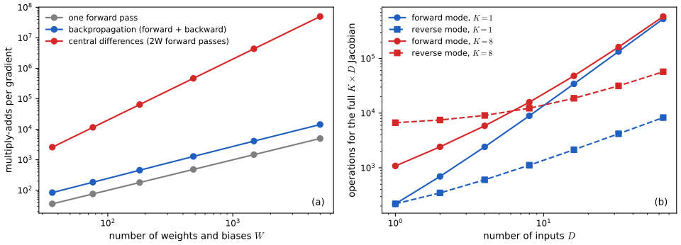
Each weight \(w_{ji}\) is used once in (8.5) (one multiply, one add). In (8.13) the term \(w_{kj}\delta_k\) is formed once for each edge out of a hidden unit, so at most once per weight (edges out of the inputs and the bias are not needed: no \(\delta\) is computed for inputs). Each derivative (8.10) is one multiplication per weight. The activation derivatives \(h'(a_j)\) cost one evaluation per unit and are often free: for tanh, \(h'=1-z^2\) reuses the stored \(z_j\) (8.16). Units are far fewer than weights in all but very sparse networks, so the total is \(\le3W+O(\text{units})\). Counted exactly by the instrumented code: on fully connected 8-\(M\)-\(M\)-4 networks the ratio (backprop)/(one forward pass) is 2.33 for \(W=36\) and 2.87 for \(W=4996\), approaching 3 from below (Figure 8.S1(a)).
p. 238 Nothing in the derivation required one activation function for all units: each unit simply uses its own \(h_j'\).
8.1.3 A simple example
See also the companion course, Section 5.3.2.
pp. 238–239 Take the two-layer network of Figure 6.9 with tanh hidden units and linear outputs. The tanh function
\[ h(a)\equiv\tanh(a) \tag{8.15} \]has the convenient derivative
\[ h'(a)=1-h(a)^2, \tag{8.16} \](since \(\tanh'=\operatorname{sech}^2=1-\tanh^2\)). With the sum-of-squares error
\[ E_n=\frac12\sum_{k=1}^K(y_k-t_k)^2, \tag{8.17} \]the forward pass is
\[ a_j=\sum_{i=0}^Dw^{(1)}_{ji}x_i, \tag{8.18} \] \[ z_j=\tanh(a_j), \tag{8.19} \] \[ y_k=\sum_{j=0}^Mw^{(2)}_{kj}z_j, \tag{8.20} \]with \(x_0=z_0=1\) for the biases. The output errors and the backpropagated hidden errors are
\[ \delta_k=y_k-t_k, \tag{8.21} \] \[ \delta_j=(1-z_j^2)\sum_{k=1}^Kw^{(2)}_{kj}\delta_k, \tag{8.22} \]and the derivatives are
\[ \frac{\partial E_n}{\partial w^{(1)}_{ji}}=\delta_jx_i,\qquad\frac{\partial E_n}{\partial w^{(2)}_{kj}}=\delta_kz_j. \tag{8.23} \]Filling the gap 8.3: the example with numbers pp. 238–239
Following one data point through every step makes the algorithm concrete. Take \(D=2\), \(M=2\), \(K=1\), the input \(\bx=(1,0.5)\), the target \(t=0.3\), and the weights (bias first)
\[\bW^{(1)}=\begin{pmatrix}0.1&0.5&-0.4\\-0.2&0.3&0.8\end{pmatrix},\qquad\bw^{(2)}=(0.05,\ 1.2,\ -0.7).\]Every step
Forward. \(a_1=0.1+0.5\cdot1-0.4\cdot0.5=0.4\) and \(a_2=-0.2+0.3+0.8\cdot0.5=0.5\); \(z_1=\tanh0.4=0.379949\), \(z_2=\tanh0.5=0.462117\); \(y=0.05+1.2\cdot0.379949-0.7\cdot0.462117=0.182457\), and \(E_n=\tfrac12(0.182457-0.3)^2=0.006908\).
Output error. \(\delta=y-t=-0.117543\).
Backward. \(\delta_1=(1-z_1^2)\,w^{(2)}_1\delta=0.855639\cdot1.2\cdot(-0.117543)=-0.120689\); \(\delta_2=(1-z_2^2)\,w^{(2)}_2\delta=0.786448\cdot(-0.7)\cdot(-0.117543)=0.064709\).
Derivatives.
| weight | bias | from \(x_1\) / \(z_1\) | from \(x_2\) / \(z_2\) |
|---|---|---|---|
| into hidden unit 1: \(\delta_1(1,x_1,x_2)\) | \(-0.120689\) | \(-0.120689\) | \(-0.060345\) |
| into hidden unit 2: \(\delta_2(1,x_1,x_2)\) | \(0.064709\) | \(0.064709\) | \(0.032355\) |
| into the output: \(\delta(1,z_1,z_2)\) | \(-0.117543\) | \(-0.044660\) | \(-0.054319\) |
Two features to notice. The output is too small, so every output weight should grow where its input is positive: all three output derivatives are negative. And hidden unit 2 connects to the output with a negative weight, so its error has the opposite sign from unit 1's. Central differences agree with all nine derivatives to \(10^{-8}\) (worked_example, checked).
Skip-layer weights \(u_{ki}\) from the inputs straight to the outputs add \(\sum_iu_{ki}x_i\) to (8.20); since \(u_{ki}\) enters only \(a_k\), \(\partial E_n/\partial u_{ki}=\delta_kx_i\) (Exercise 8.4; demo preset 4).
8.1.4 Numerical differentiation
See also the companion course, Section 5.3.3 and Filling the gap 5.6.
p. 239 Evaluating \(E_n\) once costs \(O(W)\) (Result 8.2). The alternative to backpropagation is to perturb each weight in turn. Forward (finite) differences give
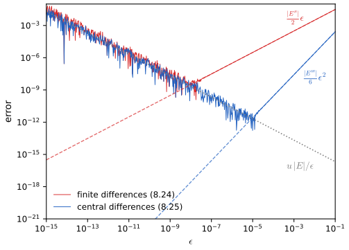
\[ \frac{\partial E_n}{\partial w_{ji}}=\frac{E_n(w_{ji}+\epsilon)-E_n(w_{ji})}{\epsilon}+O(\epsilon), \tag{8.24} \]and symmetric central differences, at twice the cost,
\[ \frac{\partial E_n}{\partial w_{ji}}=\frac{E_n(w_{ji}+\epsilon)-E_n(w_{ji}-\epsilon)}{2\epsilon}+O(\epsilon^2). \tag{8.25} \]Either way the cost is \(O(W)\) per weight and \(O(W^2)\) for the gradient, against \(O(W)\) for backpropagation; numerical derivatives remain valuable as a check of a backpropagation or autodiff implementation.
Result 8.3 (truncation and round-off: the shape of Figure 8.2) pp. 239–240, (8.24)–(8.25); Exercise 8.3
Let \(E\), as a function of one weight, have a continuous third derivative near \(w\). In exact arithmetic
\[\frac{E(w+\epsilon)-E(w)}{\epsilon}-E'(w)=\frac{\epsilon}{2}E''(\xi),\qquad\frac{E(w+\epsilon)-E(w-\epsilon)}{2\epsilon}-E'(w)=\frac{\epsilon^2}{6}E'''(\xi'),\]for some \(\xi,\xi'\) within \(\epsilon\) of \(w\). If each computed value of \(E\) carries a relative error of order the unit round-off \(u\), the total errors behave like
\[\text{forward: }\ \frac{\epsilon}{2}|E''|+\frac{2u|E|}{\epsilon},\qquad\text{central: }\ \frac{\epsilon^2}{6}|E'''|+\frac{u|E|}{\epsilon},\]which are smallest at \(\epsilon^\star=2\sqrt{u|E|/|E''|}\) (error \(2\sqrt{u|E||E''|}=O(u^{1/2})\)) and at \(\epsilon^\star=(3u|E|/|E'''|)^{1/3}\) (error \(\tfrac32u|E|/\epsilon^\star=O(u^{2/3})\)). On a log-log plot: slope 1 and slope 2 for large \(\epsilon\), slope \(-1\) for small \(\epsilon\), where both methods give the same noise.
Proof (Exercise 8.3, with the remainder terms)
Truncation. Taylor's theorem with the Lagrange remainder gives \(E(w+\epsilon)=E+\epsilon E'+\tfrac12\epsilon^2E''(\xi)\), which is the forward statement. For the central difference expand to third order on both sides: \[E(w\pm\epsilon)=E\pm\epsilon E'+\tfrac12\epsilon^2E''\pm\tfrac16\epsilon^3E'''(\xi_\pm).\] Subtracting, the even terms (\(E\) and \(\tfrac12\epsilon^2E''\)) cancel, which is the cancellation the book refers to: \(E(w+\epsilon)-E(w-\epsilon)=2\epsilon E'+\tfrac16\epsilon^3\big(E'''(\xi_+)+E'''(\xi_-)\big)\). Dividing by \(2\epsilon\), the error is \(\tfrac{\epsilon^2}{12}(E'''(\xi_+)+E'''(\xi_-))\), and since \(E'''\) is continuous the average of its two values is \(E'''(\xi')\) for some \(\xi'\) between them (intermediate value theorem): the error is \(\tfrac{\epsilon^2}{6}E'''(\xi')=O(\epsilon^2)\).
Round-off. The computer returns \(\widehat E(w\pm\epsilon)=E(w\pm\epsilon)(1+\theta_\pm)\) with \(|\theta_\pm|\) of order \(u\) (a model: a forward pass accumulates round-off, so in practice \(|\theta|\) is a modest multiple of \(u\)). The difference of the two computed values is then wrong by up to \(2u|E|\), and dividing by \(\epsilon\) (forward) or \(2\epsilon\) (central) multiplies this by \(1/\epsilon\) or \(1/(2\epsilon)\). Adding the truncation terms gives the two error models.
Best steps. For \(f(\epsilon)=A\epsilon+B/\epsilon\), \(f'=0\) at \(\epsilon^\star=\sqrt{B/A}\) with \(f(\epsilon^\star)=2\sqrt{AB}\); with \(A=|E''|/2\), \(B=2u|E|\) this is the forward result. For \(f=A\epsilon^2+B/\epsilon\), \(\epsilon^{\star3}=B/(2A)\); with \(A=|E'''|/6\), \(B=u|E|\), \(\epsilon^{\star3}=3u|E|/|E'''|\), and at the optimum \(A\epsilon^{\star2}=B/(2\epsilon^\star)\), so \(f=\tfrac32B/\epsilon^\star\).
The numbers of Figure 8.2. For the error and weight used there, \(|E|=0.190\), \(E'=0.4279\), \(E''=0.618\), \(E'''=0.159\) (the derivatives computed exactly with nested dual numbers, Section 8.2.1). The predicted best steps are \(1.2\times10^{-8}\) (forward) and \(7.4\times10^{-6}\) (central); the observed minima of the smoothed curves are at \(1.1\times10^{-8}\) and \(7.8\times10^{-6}\). The fitted slopes in the truncation regime are 1.000 and 2.000, and the leading constants \(|E''|/2\) and \(|E'''|/6\) match the observed errors to 0.01% (all checked). The observed errors at the best steps (as low as \(1.2\times10^{-10}\) and \(1.7\times10^{-13}\)) are below the worst-case model, because the individual round-off errors are random and partly cancel.
Filling the gap 8.4: gradient checking in practice, its cost, and where it fails pp. 239–240
The book recommends comparing backpropagation with central differences. Result 8.3 turns this advice into a procedure.
Derivation
Step and tolerance. In double precision use central differences with \(\epsilon\approx10^{-6}\) to \(10^{-5}\) (scaled by \(\max(1,|w_{ji}|)\)), and compare relative errors \(|g_{\rm bp}-g_{\rm fd}|/\max(|g_{\rm bp}|,|g_{\rm fd}|)\): agreement to \(10^{-7}\) or better is the signature of a correct implementation, while a bug typically shows as an error of order one. In single precision (\(u\approx6\times10^{-8}\)) the best attainable central-difference error is only about \(u^{2/3}\approx10^{-5}\) relative, so checks should be run in double precision.
Cost. Checking all \(W\) derivatives takes \(2W\) evaluations of \(E_n\), each \(O(W)\): \(O(W^2)\) work. For the 8-64-64-4 network of Figure 8.S1(a) (\(W=4996\)) that is \(5.0\times10^7\) multiply-adds against \(1.4\times10^4\) for backpropagation. A cheaper check uses a random direction \(\bv\): one central difference along \(\bv\) approximates the directional derivative \(\bv^\T\nabla E_n\) with two evaluations, which is compared with the inner product of \(\bv\) and the backpropagated gradient.
Kinks. Result 8.3 assumes smoothness. At a ReLU (or max-pooling) unit whose pre-activation is within \(\epsilon\) of the kink, \(E(w+\epsilon)\) and \(E(w-\epsilon)\) lie on different linear pieces, and the central difference returns the average of the two one-sided slopes. In demo preset 5 hidden unit 1 has \(a_1=10^{-6}\): the backpropagated derivative for the weight from \(x_1\) is 1.0347, the central difference with \(\epsilon=10^{-4}\) is 0.5260, and with \(\epsilon=10^{-8}\) it is 1.0347 again (checked). A failed check at a kink is therefore not a bug in backpropagation.
8.1.5 The Jacobian matrix
See also the companion course, Section 5.3.4 and Result 5.7.
pp. 240–242 The Jacobian of the network collects the derivatives of the outputs with respect to the inputs,
\[ J_{ki}\equiv\frac{\partial y_k}{\partial x_i}, \tag{8.26} \]each taken with the other inputs fixed. In a system of differentiable modules (Figure 8.3, a schematic, not reproduced: modules \(u\), \(v\), \(w\) in a chain, with the outputs \(\bz\) of one feeding the next), the derivative of the error with respect to a parameter \(w\) of an early module passes through the Jacobian of every later module:
\[ \frac{\partial E}{\partial w}=\sum_{k,j}\frac{\partial E}{\partial y_k}\frac{\partial y_k}{\partial z_j}\frac{\partial z_j}{\partial w}. \tag{8.27} \]The Jacobian also propagates small input errors to the outputs,
\[ \Delta y_k\simeq\sum_i\frac{\partial y_k}{\partial x_i}\Delta x_i, \tag{8.28} \]valid for small \(|\Delta x_i|\), and must be recomputed at each input because the network is nonlinear. It is computed by a backward recursion that starts like backpropagation:
\[ J_{ki}=\frac{\partial y_k}{\partial x_i}=\sum_j\frac{\partial y_k}{\partial a_j}\frac{\partial a_j}{\partial x_i}=\sum_jw_{ji}\frac{\partial y_k}{\partial a_j}, \tag{8.29} \] \[ \frac{\partial y_k}{\partial a_j}=\sum_l\frac{\partial y_k}{\partial a_l}\frac{\partial a_l}{\partial a_j}=h'(a_j)\sum_lw_{lj}\frac{\partial y_k}{\partial a_l}, \tag{8.30} \]where \(j\) runs over the units fed by input \(i\) and \(l\) over the units fed by \(j\). At the outputs, for linear units,
\[ \frac{\partial y_k}{\partial a_l}=\delta_{kl}, \tag{8.31} \]with the Kronecker delta
\[ \delta_{kl}=\begin{cases}1,&k=l,\\0,&\text{otherwise};\end{cases} \tag{8.32} \]for logistic outputs
\[ \frac{\partial y_k}{\partial a_l}=\delta_{kl}\sigma'(a_l), \tag{8.33} \]and for softmax outputs
\[ \frac{\partial y_k}{\partial a_l}=\delta_{kl}y_k-y_ky_l. \tag{8.34} \]A numerical test uses central differences in each input,
\[ \frac{\partial y_k}{\partial x_i}=\frac{y_k(x_i+\epsilon)-y_k(x_i-\epsilon)}{2\epsilon}+O(\epsilon^2), \tag{8.35} \]which takes \(2D\) forward passes, \(O(DW)\) in all.
Result 8.4 (the Jacobian by backward or forward propagation) pp. 241–242, (8.29)–(8.35); Exercise 8.5
(a) Backward: starting from \(\partial y_k/\partial a_l\) at the outputs, (8.31), (8.33) or (8.34), the recursion (8.30) in reverse topological order and then (8.29) give row \(k\) of \(\bJ\). One backward pass per output: \(O(KW)\) for the whole Jacobian.
(b) Forward: with \(G_{ji}=\partial a_j/\partial x_i\), \(G_{ji}=w_{ji}\) for first-layer units, and in topological order
\[G_{li}=\sum_jw_{lj}h'(a_j)G_{ji},\qquad J_{ki}=\sum_l\frac{\partial y_k}{\partial a_l}G_{li}.\]One forward pass per input: \(O(DW)\).
(c) Layered form: \(\bJ=\bS^{(L)}\bW^{(L)}\bS^{(L-1)}\bW^{(L-1)}\cdots\bS^{(1)}\bW^{(1)}\), with \(\bS^{(l)}=\diag(h'(\ba^{(l)}))\) for hidden layers and \(\bS^{(L)}=\partial\by/\partial\ba^{(L)}\). The backward recursion multiplies this product from the left, the forward one from the right.
(d) The approximation (8.28) has error \(O(\|\Delta\bx\|^2)\) when \(\by\) is twice differentiable.
Proof
(8.33) and (8.34). A logistic output \(y_k=\sigma(a_k)\) depends only on its own \(a_k\), so \(\partial y_k/\partial a_l=\delta_{kl}\sigma'(a_l)=\delta_{kl}y_l(1-y_l)\). For softmax, \(y_k=e^{a_k}/S\) with \(S=\sum_me^{a_m}\), and \(\partial S/\partial a_l=e^{a_l}\), so by the quotient rule \[\frac{\partial y_k}{\partial a_l}=\frac{\delta_{kl}e^{a_k}S-e^{a_k}e^{a_l}}{S^2}=\delta_{kl}y_k-y_ky_l.\]
(a). (8.29) is the chain rule through the units fed by input \(i\), using \(\partial a_j/\partial x_i=w_{ji}\) from (8.5). (8.30) is the chain rule through the children \(l\) of \(j\), with \(\partial a_l/\partial a_j=w_{lj}h'(a_j)\) exactly as in Result 8.1; the recursion is well defined in reverse topological order by the same induction. Each pass touches each weight a bounded number of times: \(O(W)\).
(b) (Exercise 8.5). Every path from input \(i\) to unit \(l\) passes through the parents \(j\) of \(l\), and \(a_l=\sum_jw_{lj}h(a_j)\), so \(\partial a_l/\partial x_i=\sum_jw_{lj}h'(a_j)\,\partial a_j/\partial x_i\) (for a parent that is an input, the term is \(w_{li}\) if it is input \(i\) and 0 otherwise). In topological order the right side is known. The last step is the chain rule through the output pre-activations.
(c). In a layered network \(\partial\ba^{(l)}/\partial\ba^{(l-1)}=\bW^{(l)}\diag(h'(\ba^{(l-1)}))\) and \(\partial\ba^{(1)}/\partial\bx=\bW^{(1)}\); the chain rule multiplies these. Evaluating the product as \(\be_k^\T\bS^{(L)}\bW^{(L)}\cdots\) (row vectors times matrices, from the left) is (a); evaluating \(\cdots\bS^{(1)}\bW^{(1)}\be_i\) (matrices times column vectors, from the right) is (b).
(d). Taylor's theorem: \(\by(\bx+\Delta\bx)=\by(\bx)+\bJ\Delta\bx+O(\|\Delta\bx\|^2)\). For a 4-6-5-3 network, shrinking \(\Delta\bx\) tenfold reduced the error of (8.28) by a factor 99.4. Backward, forward and autograd Jacobians agree to \(10^{-12}\) for linear, logistic and softmax outputs, and (8.35) to \(10^{-8}\) (checked).
Filling the gap 8.5: backpropagating through a module never needs its Jacobian pp. 240–241, (8.27)
Derivation
In (8.27) the sum over \(k\) can be done first: \(\partial E/\partial z_j=\sum_k(\partial E/\partial y_k)(\partial y_k/\partial z_j)\), i.e. the row vector \(\partial E/\partial\bz=(\partial E/\partial\by)\,\bJ\), a vector-Jacobian product. For a network module this product is exactly what one backward pass computes when the output deltas are set to \(\partial E/\partial\by\) (Result 8.4(c) multiplied from the left by a row vector), at cost \(O(W)\), whereas forming \(\bJ\) first would cost \(K\) backward passes. Chaining modules therefore costs one backward pass per module, not one per output of each module: this is backpropagation lifted from units to modules, and it is how every deep-learning library composes layers. The full Jacobian is needed only when it is the object of interest, for example for the sensitivity analysis (8.28).
8.1.6 The Hessian matrix
See also the companion course, Section 5.4 (the Hessian matrix, all six subsections), and here Section 7.1.1 (the Hessian in the local quadratic approximation).
pp. 242–243 Backpropagation also yields second derivatives,
\[ \frac{\partial^2E}{\partial w_{ji}\partial w_{lk}}, \tag{8.36} \]which, with all weights and biases in one vector \(\bw\), form the Hessian
\[ H_{ij}=\frac{\partial^2E}{\partial w_i\partial w_j},\qquad i,j\in\{1,\ldots,W\}. \tag{8.37} \]It appears in second-order optimisation, in Bayesian treatments (the Laplace approximation) and in compressing large models by reducing the precision of weights (Shen et al., 2019). Its size makes it expensive: \(W^2\) entries, \(O(W^2)\) work per data point even with the extended backpropagation of Bishop (1992), and \(O(W^3)\) to invert. Products \(\bv^\T\bH\) cost only \(O(W)\) (Møller, 1993; Pearlmutter, 1994; Result 8.7). Keeping only the diagonal needs \(O(W)\) storage and inversion, but its evaluation costs \(O(W^2)\) unless approximated further (Becker and LeCun, 1989), and real Hessians have large off-diagonal terms (see the companion course's Result 5.8).
pp. 243–244 A better approximation starts from the sum-of-squares error with one output,
\[ E=\frac12\sum_{n=1}^N(y_n-t_n)^2, \tag{8.38} \]whose Hessian is
\[ \bH=\nabla\nabla E=\sum_{n=1}^N\nabla y_n(\nabla y_n)^\T+\sum_{n=1}^N(y_n-t_n)\nabla\nabla y_n. \tag{8.39} \]The second sum is small for a well-trained network whose outputs are close to the targets, and averages out in general if the residuals \(y_n-t_n\) are zero-mean noise uncorrelated with \(\nabla\nabla y_n\). Dropping it gives the Levenberg–Marquardt or outer-product approximation
\[ \bH\simeq\sum_{n=1}^N\nabla a_n\nabla a_n^\T, \tag{8.40} \](here \(a_n=y_n\) for a linear output). It needs only first derivatives, \(O(W)\) per point by backpropagation, then \(O(W^2)\) to form; the book stresses that it is likely to be valid only for a network that has been trained. For a logistic output with the cross-entropy,
\[ \bH\simeq\sum_{n=1}^Ny_n(1-y_n)\nabla a_n\nabla a_n^\T, \tag{8.41} \]and an analogous result holds for softmax outputs (Exercises 8.10, 8.11). It also gives a one-pass algorithm for the inverse Hessian (Hassibi and Stork, 1993; Exercise 8.12).
Result 8.5 (the outer-product approximation: derivation, positivity and when it is exact) pp. 243–244, (8.38)–(8.41); Exercises 8.8, 8.10, 8.11
Let \(\ba_n\in\R^K\) be the output pre-activations for data point \(n\), \(\bB_n=\partial\ba_n/\partial\bw\) (a \(K\times W\) matrix of first derivatives), and let \(E=\sum_nE_n\) be a canonical error, with \(\partial E_n/\partial\ba_n=\by_n-\bt_n\) and \(\bM_n=\partial^2E_n/\partial\ba_n\partial\ba_n^\T\). Then
\[\bH=\underbrace{\sum_n\bB_n^\T\bM_n\bB_n}_{\HOP}+\sum_n\sum_k(y_{nk}-t_{nk})\nabla\nabla a_{nk},\qquad\bM_n=\begin{cases}\bI&\text{linear, sum-of-squares},\\\diag(y_{nk}(1-y_{nk}))&\text{logistic},\\\diag(\by_n)-\by_n\by_n^\T&\text{softmax}.\end{cases}\](i) \(\HOP\) is positive semi-definite, whatever \(\bw\) and the data. (ii) \(\HOP=\bH\) exactly when every residual \(y_{nk}-t_{nk}\) is zero, and also, whatever the residuals, on any block of weights in which every \(a_{nk}\) is affine (for example the weights of the output layer). (iii) For one linear output this is (8.39)–(8.40); for several, \(\HOP=\sum_n\sum_k\nabla y_{nk}\nabla y_{nk}^\T\) (Exercise 8.8); for one logistic output it is (8.41) (Exercise 8.10).
Proof
The decomposition. \(E_n\) depends on \(\bw\) only through \(\ba_n\). The chain rule gives \(\partial E_n/\partial w_r=\sum_k(y_{nk}-t_{nk})\,\partial a_{nk}/\partial w_r\). Differentiate again with respect to \(w_s\) by the product rule: the derivative of \(y_{nk}-t_{nk}\) is \(\sum_l(\partial y_{nk}/\partial a_{nl})(\partial a_{nl}/\partial w_s)=\sum_lM_{n,kl}B_{n,ls}\), because \(\partial^2E_n/\partial a_k\partial a_l=\partial y_k/\partial a_l\) for canonical pairs, and the derivative of \(\partial a_{nk}/\partial w_r\) is \(\partial^2a_{nk}/\partial w_r\partial w_s\). So \[\frac{\partial^2E_n}{\partial w_r\partial w_s}=\sum_{k,l}B_{n,kr}M_{n,kl}B_{n,ls}+\sum_k(y_{nk}-t_{nk})\frac{\partial^2a_{nk}}{\partial w_r\partial w_s},\] and summing over \(n\) gives the decomposition. The three \(\bM_n\) are \(\partial\by/\partial\ba\) from (8.31), (8.33) and (8.34). With \(K=1\) and a linear output, \(\bM_n=1\) and \(a_n=y_n\): (8.39), and dropping the second sum gives (8.40). With one logistic output, \(\bM_n=y_n(1-y_n)\): (8.41).
(i). \(\bv^\T\HOP\bv=\sum_n(\bB_n\bv)^\T\bM_n(\bB_n\bv)\), so it suffices that each \(\bM_n\) is positive semi-definite. For the identity and a nonnegative diagonal this is clear. For softmax, with \(\bc=\bB_n\bv\), \(\bc^\T(\diag\by-\by\by^\T)\bc=\sum_ky_kc_k^2-(\sum_ky_kc_k)^2\), the variance of \(c\) under the distribution \(\by\), which is \(\ge0\). The exact \(\bH\) has no such guarantee: at a random point of a 2-3-2 network its smallest eigenvalue was \(-3.51\) while that of \(\HOP\) was \(0\) to round-off (checked).
(ii). The difference \(\bH-\HOP\) is the residual sum, which vanishes term by term if every residual is zero, and on any block where \(\nabla\nabla a_{nk}=\bzero\). The output-layer weights enter \(a_{nk}\) linearly, so the output-layer block of \(\bH\) equals that of \(\HOP\) at any residuals (checked to \(10^{-12}\)). For a model linear in all its parameters (linear regression) \(\HOP\) is the exact Hessian, \(\Phi^\T\Phi\).
Numerical tests. When the targets are set equal to the outputs, \(\HOP\) matches autograd's Hessian to \(10^{-11}\) for sum-of-squares with two outputs, logistic, and softmax with three outputs.
Naming: \(\HOP\) is the Gauss–Newton matrix (generalised Gauss–Newton for the cross-entropies); the Levenberg–Marquardt method uses \(\HOP+\lambda\bI\) with an adaptive damping \(\lambda\). For the cross-entropies \(\HOP\) also equals the Fisher information of the model's predictive distribution.
Filling the gap 8.6: the averaging argument, made exact, and when it fails (Exercise 8.9) pp. 243–244; Exercise 8.9
The book justifies dropping the residual term because \(y_n-t_n\) has zero mean and is "uncorrelated" with \(\nabla\nabla y_n\). Here is what that means and how fast it works.
Derivation
Population version (Exercise 8.9). For \(E(\bw)=\frac12\iint\{y(\bx,\bw)-t\}^2p(\bx,t)\,\d\bx\,\d t\), differentiating twice under the integral and doing the \(t\)-integral first (\(\int(y-t)p(t\given\bx)\,\d t=y-\E[t\given\bx]\)), \[\frac{\partial^2E}{\partial w_r\partial w_s}=\int\frac{\partial y}{\partial w_r}\frac{\partial y}{\partial w_s}p(\bx)\,\d\bx+\int\big(y(\bx,\bw)-\E[t\given\bx]\big)\frac{\partial^2y}{\partial w_r\partial w_s}p(\bx)\,\d\bx.\] At weights \(\bws\) with \(y(\bx,\bws)=\E[t\given\bx]\) for all \(\bx\), the minimiser of (8.78) by (4.37) (Section 4.2), the second integral vanishes exactly and (8.79) follows. This needs the network to represent the regression function; otherwise the best network has a systematic bias \(b(\bx)=y(\bx,\bws)-\E[t\given\bx]\ne0\).
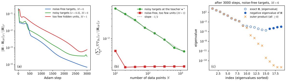
Finite samples at \(\bws\). Write \(t_n=\E[t\given\bx_n]+\varepsilon_n\) with independent zero-mean noise of variance \(\sigma^2\). The residual term is \(\bR_N=\sum_n(y_n-t_n)\nabla\nabla y_n=-\sum_n\varepsilon_n\nabla\nabla y(\bx_n)\): given the inputs it has mean \(\bzero\), and each entry has variance \(\sigma^2\sum_n(\partial^2y_n/\partial w_r\partial w_s)^2=O(N)\). So \(\|\bR_N\|=O(\sigma\sqrt N)\), while \(\HOP=\sum_n\nabla y_n\nabla y_n^\T\) grows like \(N\): the ratio falls like \(N^{-1/2}\). For a fitted network, the empirical minimiser differs from \(\bws\) by \(O(N^{-1/2})\), which changes \(\bR_N/N\) by the same order.
With a bias. If the model is too small, \(\bR_N/N\to\int b(\bx)\nabla\nabla y\,p(\bx)\,\d\bx\), which is not zero in general: the residuals are correlated with the curvature, and no amount of data removes the term.
Numbers (Figure 8.S2, 1-\(M\)-1 tanh networks on \(t=\sin\pi x\) plus noise). (a) After 3000 Adam steps, \(\|\bH-\HOP\|_F/\|\bH\|_F\) is 0.21 at initialisation and \(7.1\times10^{-5}\) (noise-free, \(M=6\)), \(3.1\times10^{-4}\) (\(\sigma=0.3\)) and \(7.7\times10^{-4}\) (\(M=1\)). (b) At a teacher network with noisy targets, \(\|\bR_N\|_F/\|\HOP\|_F\) falls with slope \(-0.51\) from \(N=10\) to 1280, while for \(M=1\) it stays at \(2.1\times10^{-3}\). Averaged over 4000 noise draws, \(\bR_N\) is \(0.008\) times a single draw: zero mean, as claimed. (c) Even for the noise-free fit, the four smallest eigenvalues of \(\bH\) are negative (down to \(-3.4\times10^{-4}\)), while \(\HOP\) is positive semi-definite: the approximation is excellent in the stiff directions and unreliable in the flat ones, which is where the Frobenius norm does not look. All checked.
Result 8.6 (exact Hessian of a two-layer network, with skip-layer weights) p. 243; Exercises 8.6, 8.7
For the network of Section 8.1.3 with any canonical output pair, let \(\delta_k=\partial E_n/\partial a_k\) and \(M_{kk'}=\partial^2E_n/\partial a_k\partial a_{k'}\) (8.77), \(x_0=z_0=1\), and \(I_{jj'}\) the identity. Then
\[\frac{\partial^2E_n}{\partial w^{(2)}_{kj}\partial w^{(2)}_{k'j'}}=z_jz_{j'}M_{kk'},\] \[\frac{\partial^2E_n}{\partial w^{(1)}_{ji}\partial w^{(1)}_{j'i'}}=x_ix_{i'}\Big[h''(a_j)I_{jj'}\sum_kw^{(2)}_{kj}\delta_k+h'(a_j)h'(a_{j'})\sum_{k,k'}w^{(2)}_{kj}w^{(2)}_{k'j'}M_{kk'}\Big],\] \[\frac{\partial^2E_n}{\partial w^{(1)}_{ji}\partial w^{(2)}_{kj'}}=x_ih'(a_j)\Big[\delta_kI_{jj'}+z_{j'}\sum_{k'}w^{(2)}_{k'j}M_{kk'}\Big].\]With skip-layer weights \(u_{ki}\) (Exercise 8.7) three more blocks appear:
\[\frac{\partial^2E_n}{\partial u_{ki}\partial u_{k'i'}}=M_{kk'}x_ix_{i'},\quad\frac{\partial^2E_n}{\partial u_{ki}\partial w^{(2)}_{k'j}}=M_{kk'}z_jx_i,\quad\frac{\partial^2E_n}{\partial u_{ki}\partial w^{(1)}_{ji'}}=x_ix_{i'}h'(a_j)\sum_{k'}M_{kk'}w^{(2)}_{k'j}.\]Every entry costs \(O(1)\) once the forward quantities, the \(\delta_k\) and \(\bM\) are known (for the double sums, precompute \(\bW^{(2)\T}\bM\bW^{(2)}\), \(O(KM^2)\)): \(O(W^2)\) per data point, the optimal order for an object with \(W^2\) entries.
Proof (Exercises 8.6 and 8.7)
Start from the gradients: \(\partial E_n/\partial w^{(2)}_{kj}=\delta_kz_j\), \(\partial E_n/\partial w^{(1)}_{ji}=x_ih'(a_j)\sum_kw^{(2)}_{kj}\delta_k\), \(\partial E_n/\partial u_{ki}=\delta_kx_i\). Two facts do all the work: \(\partial\delta_k/\partial(\text{weight})=\sum_{k'}M_{kk'}\,\partial a_{k'}/\partial(\text{weight})\), and the derivatives of the output pre-activations are \(\partial a_{k'}/\partial w^{(2)}_{k''j'}=I_{k'k''}z_{j'}\), \(\partial a_{k'}/\partial w^{(1)}_{j'i'}=w^{(2)}_{k'j'}h'(a_{j'})x_{i'}\), \(\partial a_{k'}/\partial u_{k''i'}=I_{k'k''}x_{i'}\).
Second layer. \(z_j\) does not depend on second-layer weights, so the derivative of \(\delta_kz_j\) with respect to \(w^{(2)}_{k'j'}\) is \(z_j\sum_{k''}M_{kk''}I_{k''k'}z_{j'}=z_jz_{j'}M_{kk'}\).
First layer. Differentiate \(x_ih'(a_j)\sum_kw^{(2)}_{kj}\delta_k\) with respect to \(w^{(1)}_{j'i'}\). The factor \(h'(a_j)\) changes only if \(j'=j\), by \(h''(a_j)x_{i'}\); this gives the first term. Each \(\delta_k\) changes by \(\sum_{k'}M_{kk'}w^{(2)}_{k'j'}h'(a_{j'})x_{i'}\); this gives the second.
Mixed. Differentiate \(\delta_kz_{j'}\) with respect to \(w^{(1)}_{ji}\): \(z_{j'}\) changes only if \(j'=j\), by \(h'(a_j)x_i\), giving \(\delta_kI_{jj'}h'(a_j)x_i\); \(\delta_k\) changes by \(\sum_{k'}M_{kk'}w^{(2)}_{k'j}h'(a_j)x_i\), multiplied by \(z_{j'}\).
Skip layer. Differentiate \(\delta_kx_i\) (the \(x_i\) are constants): the change of \(\delta_k\) with respect to \(u_{k'i'}\), \(w^{(2)}_{k'j}\) and \(w^{(1)}_{ji'}\) is \(M_{kk'}x_{i'}\), \(M_{kk'}z_j\) and \(\sum_{k'}M_{kk'}w^{(2)}_{k'j}h'(a_j)x_{i'}\) respectively.
Numerical tests. The assembled matrix equals autograd's Hessian to \(10^{-11}\) for linear outputs (\(W=26\)), softmax outputs (\(W=31\)), and with skip layers for linear (\(W=32\)), logistic (\(W=24\)) and softmax (\(W=40\)) outputs.
Errata (solutions manual, Solution 8.6). In (275) the factor must be \(h'(a_{j'})\), not \(h'(a_j)\); the text then says "we obtain (??)" and never writes the first-layer block; and the last line of the mixed block drops the factor \(z_{j'}\) in front of \(\sum_{k'}w^{(2)}_{k'j}M_{kk'}\) (it is present one line earlier). Without \(z_{j'}\) one entry of the test network comes out as \(0.01428\) instead of the correct \(-0.00783\) (checked against autograd). Solution 8.7 is correct but refers to "Section ??".
Algorithm 8.2 (the inverse outer-product Hessian in one pass) p. 244; Exercise 8.12
Set \(\bH_0^{-1}=\alpha^{-1}\bI\). For each data point (and each output) with gradient vector \(\bb=\nabla a_{n}\) (times \(\sqrt{y_n(1-y_n)}\) for a logistic output),
\[\bH_{L+1}^{-1}=\bH_L^{-1}-\frac{(\bH_L^{-1}\bb)(\bH_L^{-1}\bb)^\T}{1+\bb^\T\bH_L^{-1}\bb}.\]After all the data, the result is exactly \((\HOP+\alpha\bI)^{-1}\). Cost: \(O(W^2)\) per vector \(\bb\), one pass through the data, no matrix inversion.
Proof
\(\bH_{L+1}=\bH_L+\bb\bb^\T\) by (8.40), and the update is (8.80) with \(\bM=\bH_L\), \(\bv=\bb\), using the symmetry of \(\bH_L^{-1}\). (8.80) itself: multiply \(\bM+\bv\bv^\T\) by the right side; with \(s=\bv^\T\bM^{-1}\bv\) the product is \(\bI+\bv\bv^\T\bM^{-1}-\frac{\bv\bv^\T\bM^{-1}+s\,\bv\bv^\T\bM^{-1}}{1+s}=\bI\). It is the rank-one case of the Woodbury identity (Toolkit, Section 3.3; companion course Result 5.10). By induction \(\bH_N=\alpha\bI+\sum\bb\bb^\T=\HOP+\alpha\bI\). Checked: agreement with the direct inverse to \(3\times10^{-11}\) for every \(\alpha\ge10^{-5}\).
Filling the gap 8.7: what the initial \(\alpha\) really does Exercise 8.12
Exercise 8.12 says the results are "not particularly sensitive" to \(\alpha\). That holds only in a specific regime, which networks often miss.
Derivation
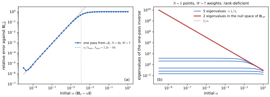
The algorithm returns \((\HOP+\alpha\bI)^{-1}\) exactly. In the eigenbasis of \(\HOP\) (eigenvalues \(\lambda_i\ge0\)) this has eigenvalues \(1/(\lambda_i+\alpha)\) against \(1/\lambda_i\), a relative change \(\alpha/(\lambda_i+\alpha)\). So the result approximates \(\HOP^{-1}\) to relative accuracy about \(\alpha/\lambda_{\min}\), and is insensitive to \(\alpha\) only if \(\alpha\ll\lambda_{\min}(\HOP)\).
Ill-conditioning. Network Hessians are badly conditioned. For the 1-2-1 network of Figure 8.S4 (\(W=7\), \(N=30\)), \(\lambda_{\min}=1.2\times10^{-4}\) against \(\lambda_{\max}=1.2\times10^3\), so \(\alpha\) must be below about \(10^{-6}\) for 1% accuracy; the observed error follows \(\alpha/\lambda_{\min}\) over five decades. Very small \(\alpha\) brings its own problem: the recursion starts from \(\alpha^{-1}\bI\) and subtracts large rank-one terms, and round-off grows like \(u\lambda_{\max}/\alpha\) (\(2.8\times10^{-6}\) at \(\alpha=10^{-10}\), checked).
Rank deficiency. If \(NK<W\), \(\HOP\) is singular: \(W-NK\) eigenvalues are zero, and the result has \(W-NK\) eigenvalues exactly \(1/\alpha\) (Figure 8.S4(b), \(N=5\), \(W=7\), checked). The output is then dominated by \(\alpha\): the choice of \(\alpha\) is not a numerical detail but a modelling decision, the precision of a Gaussian prior on the weights in the Laplace approximation (Chapter 5 of the companion course, Result 5.20).
Result 8.7 (Hessian-vector products in \(O(W)\): the R-operator) p. 243 (Møller, 1993; Pearlmutter, 1994)
Define \(\Rop\{f\}=\frac{\d}{\d r}f(\bw+r\bv)\big|_{r=0}\) for any quantity \(f\) computed from \(\bw\). Then \(\Rop\{\nabla E\}=\bH\bv\), and applying \(\Rop\) to every line of the forward and backward passes gives \(\bH\bv\) in one extended forward and one extended backward pass, \(O(W)\) operations. For the two-layer network of Section 8.1.3 (any canonical outputs, skip weights \(\bU\) optional), with \(\bv\) split like \(\bw\) into \(\bv^{(1)},\bv^{(2)},\bv^{(u)}\):
\[\Rop\{a_j\}=\sum_iv^{(1)}_{ji}x_i,\quad\Rop\{z_j\}=h'(a_j)\Rop\{a_j\},\quad\Rop\{a_k\}=\sum_j\big(w^{(2)}_{kj}\Rop\{z_j\}+v^{(2)}_{kj}z_j\big)+\sum_iv^{(u)}_{ki}x_i,\] \[\Rop\{\delta_k\}=\sum_{k'}M_{kk'}\Rop\{a_{k'}\},\quad\Rop\{\delta_j\}=h''(a_j)\Rop\{a_j\}\sum_kw^{(2)}_{kj}\delta_k+h'(a_j)\sum_kv^{(2)}_{kj}\delta_k+h'(a_j)\sum_kw^{(2)}_{kj}\Rop\{\delta_k\},\] \[(\bH\bv)_{w^{(1)}_{ji}}=x_i\Rop\{\delta_j\},\qquad(\bH\bv)_{w^{(2)}_{kj}}=\Rop\{\delta_k\}z_j+\delta_k\Rop\{z_j\},\qquad(\bH\bv)_{u_{ki}}=\Rop\{\delta_k\}x_i,\]summed over the data points. A finite-difference alternative is \(\bH\bv\approx[\nabla E(\bw+\epsilon\bv)-\nabla E(\bw-\epsilon\bv)]/(2\epsilon)\), two gradients, error \(O(\epsilon^2)\). Because \(\bH\) is symmetric, \(\bv^\T\bH=(\bH\bv)^\T\).
Proof
\(\frac{\d}{\d r}\frac{\partial E}{\partial w_i}(\bw+r\bv)\big|_{r=0}=\sum_j\frac{\partial^2E}{\partial w_i\partial w_j}v_j=(\bH\bv)_i\): \(\Rop\) is a directional derivative, so it is linear and obeys the product and chain rules, with \(\Rop\{w_i\}=v_i\) and \(\Rop\{x_i\}=0\). The backpropagation equations compute \(\nabla E\) exactly as a composition of sums, products and elementary functions of \(\bw\); applying \(\Rop\) to each of them line by line gives the stated equations (for example \(\Rop\{h(a_j)\}=h'(a_j)\Rop\{a_j\}\), and \(\Rop\{\delta_k\}=\sum_{k'}(\partial\delta_k/\partial a_{k'})\Rop\{a_{k'}\}\) with \(\partial\delta_k/\partial a_{k'}=M_{kk'}\)). Each extended line costs a constant multiple of the original one, so the total is \(O(W)\). For the finite difference, apply Result 8.3 to each component of \(r\mapsto\nabla E(\bw+r\bv)\). Numerical tests: the R-operator agrees with \(\bH\bv\) from the exact Hessian to \(10^{-11}\) for five output types and skip settings, and the finite difference to \(10^{-8}\). The same equations without skip weights are the companion course's Algorithm 5.3.
8.2 Automatic Differentiation
See also the companion course, Section 5.3.3 (efficiency of backpropagation), and here Section 7.2.1 (why gradients are worth their cost).
pp. 244–246 There are four ways to obtain the gradient of a network's error. (1) Derive the backward equations by hand and code them: efficient and exact, but slow to write, error-prone, and duplicated work whenever the architecture changes. (2) Finite differences: only the forward code is needed, accuracy is limited (Result 8.3), which matters little for noisy stochastic gradients, but the cost is \(O(W^2)\); they remain the standard check. (3) Symbolic differentiation: computer algebra applies the rules of calculus mechanically and returns expressions, exact and free of human error, but the expressions can become exponentially longer than the function (expression swell) and the method needs a closed-form expression, excluding loops, branches, recursion and procedure calls. (4) Automatic differentiation (autodiff; Baydin et al., 2018): from the code of the forward computation, generate code that evaluates the derivatives, reusing the intermediate values of the forward computation; exact to machine precision, as efficient as hand-written backpropagation, and indifferent to control flow because it differentiates the operations actually executed.
The redundancy of symbolic differentiation is visible already in a product,
\[ f(x)=u(x)v(x), \tag{8.42} \] \[ f'(x)=u'(x)v(x)+u(x)v'(x), \tag{8.43} \]where \(u\) and \(v\) are each needed twice. For a two-layer "network" with one input,
\[ z=h(w_1x+b_1), \tag{8.44} \] \[ y=h(w_2z+b_2), \tag{8.45} \]with the soft ReLU
\[ \zeta(a)=\ln(1+\exp(a)), \tag{8.46} \](the book writes \(h\) in (8.44)–(8.47) for this \(\zeta\)) the function is
\[ y(x)=h\big(w_2h(w_1x+b_1)+b_2\big), \tag{8.47} \]and its symbolic derivative with respect to \(w_1\) is
\[ \frac{\partial y}{\partial w_1}=\frac{w_2x\exp\big(w_1x+b_1+b_2+w_2\ln[1+e^{w_1x+b_1}]\big)}{\big(1+e^{w_1x+b_1}\big)\big(1+\exp(b_2+w_2\ln[1+e^{w_1x+b_1}])\big)}, \tag{8.48} \]longer than the function and with \(w_1x+b_1\) computed three times. (Exercise 8.13; the formula as printed agrees with reverse-mode autodiff to \(10^{-14}\) at two test points, checked.)
Filling the gap 8.8: how fast expressions swell, and why autodiff does not (Exercise 8.14) pp. 245–246; Exercises 8.13, 8.14
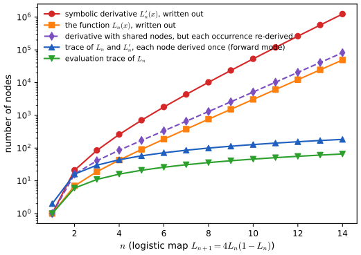
The book shows swell by example. The logistic map \(L_{n+1}=4L_n(1-L_n)\), \(L_1=x\), makes it exact.
Derivation
The function, written out. Substituting \(L_n\) twice into \(4\cdot(L_n\cdot(1-L_n))\) gives an expression tree with \(s_{n+1}=2s_n+5\) nodes (the two copies of \(L_n\), the constants 4 and 1, and three operations), \(s_1=1\), so \(s_n=6\cdot2^{n-1}-5\): the written-out function is already exponential. Simplification helps only partly (\(L_4=64x(1-x)(1-2x)^2(1-8x+8x^2)^2\) is a degree-8 polynomial; \(L_n\) has degree \(2^{n-1}\)).
The derivative, written out. The product rule turns \(4\cdot(L(1-L))\) into \(0\cdot(\ldots)+4\cdot\big(L'(1-L)+L\,(0-L')\big)\), which contains \(L_n\) twice and \(L_n'\) twice: \(d_{n+1}=2d_n+4s_n+15\), \(d_1=1\). Solving the linear recurrence, \(d_n=(6n-8)\,2^n+5\), so \(d_n/s_n\to2n\): the derivative is longer than the function by a factor that itself grows with \(n\). For \(n=12\): 12,283 nodes for \(L_{12}\), 262,149 for \(L_{12}'\) (computed by the code's small algebra system and matching the formulas).
Sharing is the cure. Store each sub-expression once (a directed acyclic graph instead of a tree): the evaluation trace of \(L_n\) has \(1+5(n-1)\) nodes, linear in \(n\). Sharing the function alone is not enough: if the derivative of a shared node is re-derived at each of its occurrences, the derivative graph still doubles at every step. If the derivative of each node is built once and reused, which is exactly forward-mode automatic differentiation, the trace of \(L_n\) together with \(L_n'\) has \(2+14(n-1)\) nodes (156 for \(n=12\)). Figure 8.S3 plots all five counts. The manual's explicit \(L_4'\) (its (308)) agrees with the forward-mode derivative at \(x=0.3\), \(L_4'(0.3)=1.3090816\) (checked).
p. 246 The key idea of autodiff is to augment the code that computes a function with extra variables, accumulated during execution, that hold derivatives. There are two principal forms: forward mode, conceptually the simpler, and reverse mode.
8.2.1 Forward-mode automatic differentiation
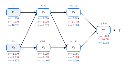
pp. 246–249 Each intermediate primal variable \(z_i\) is paired with a tangent variable \(\dot z_i\), the derivative of \(z_i\) with respect to a chosen input, and the code propagates the pairs \((z_i,\dot z_i)\). Every function is built from elementary operations (arithmetic, negation, exp, log, trigonometric functions) whose derivatives are known. Take
\[ f(x_1,x_2)=x_1x_2+\exp(x_1x_2)-\sin(x_2). \tag{8.49} \]Its evaluation trace (Figure 8.4) defines the primal variables
\[ v_1=x_1, \tag{8.50} \] \[ v_2=x_2, \tag{8.51} \] \[ v_3=v_1v_2, \tag{8.52} \] \[ v_4=\sin(v_2), \tag{8.53} \] \[ v_5=\exp(v_3), \tag{8.54} \] \[ v_6=v_3-v_4, \tag{8.55} \] \[ v_7=v_5+v_6. \tag{8.56} \]For \(\partial f/\partial x_1\), set \(\dot v_i=\partial v_i/\partial x_1\); the chain rule over the parents \(\pa(i)\) of node \(i\) gives
\[ \dot v_i=\frac{\partial v_i}{\partial x_1}=\sum_{j\in\pa(i)}\frac{\partial v_j}{\partial x_1}\frac{\partial v_i}{\partial v_j}=\sum_{j\in\pa(i)}\dot v_j\frac{\partial v_i}{\partial v_j}, \tag{8.57} \]and here
\[ \dot v_1=1, \tag{8.58} \] \[ \dot v_2=0, \tag{8.59} \] \[ \dot v_3=v_1\dot v_2+\dot v_1v_2, \tag{8.60} \] \[ \dot v_4=\dot v_2\cos(v_2), \tag{8.61} \] \[ \dot v_5=\dot v_3\exp(v_3), \tag{8.62} \] \[ \dot v_6=\dot v_3-\dot v_4, \tag{8.63} \] \[ \dot v_7=\dot v_5+\dot v_6. \tag{8.64} \]Executing the primal and tangent equations together for given \(x_1,x_2\) ends with \(\dot v_7=\partial f/\partial x_1\).
Erratum. The book says the computation runs "until we obtain \(\dot v_5\), which is the required derivative". It is \(\dot v_7\): at \((1,2)\), \(\dot v_5=2e^2=14.78\) while \(\partial f/\partial x_1=x_2+x_2e^{x_1x_2}=2+2e^2=16.78=\dot v_7\) (checked; Exercise 8.17).
Definition 8.2 (dual numbers) Section 8.2.1
A dual number is \(a+b\varepsilon\) with real \(a,b\) and a symbol \(\varepsilon\) obeying \(\varepsilon^2=0\). They add and multiply like polynomials in \(\varepsilon\): \((a+b\varepsilon)(c+d\varepsilon)=ac+(ad+bc)\varepsilon\), and \(1/(c+d\varepsilon)=1/c-(d/c^2)\varepsilon\) for \(c\ne0\). A differentiable function is extended by \(f(a+b\varepsilon)=f(a)+f'(a)\,b\,\varepsilon\). Forward mode is the evaluation of the original program on dual numbers: the primal is the real part, the tangent the \(\varepsilon\)-part.
Result 8.8 (forward mode: correctness, Jacobian-vector products and cost) pp. 247–249, (8.57), (8.66), (8.67); Exercises 8.15, 8.18
(a) For any evaluation trace and any seed \(\dot\bx\), the tangents computed by (8.57) in topological order are \(\dot v_i=\sum_j(\partial v_i/\partial x_j)\dot x_j\), the directional derivative of \(v_i\) along \(\dot\bx\). Running the program on dual numbers \(x_j+\dot x_j\varepsilon\) produces exactly these tangents.
(b) Seeding \(\dot\bx=\be_i\) gives column \(i\) of the \(K\times D\) Jacobian (8.66) in one pass; seeding \(\dot\bx=\br\) gives \(\bJ\br\) (8.67) in one pass (Exercise 8.18). The full Jacobian takes \(D\) passes.
(c) Each elementary operation with at most two arguments adds at most three arithmetic operations, plus one evaluation of a derivative \(f'\), for its tangent; a forward-mode pass therefore costs a small constant multiple of one function evaluation, and needs no storage beyond the current pairs.
Proof
(a) By induction in topological order. For an input, \(\dot v_j=\dot x_j\) by the seed. For node \(i\), \(v_i=\phi_i((v_j)_{j\in\pa(i)})\), and every \(v_j\) with \(j\in\pa(i)\) is a differentiable function of \(\bx\) whose directional derivative is \(\dot v_j\) by the induction hypothesis; the multivariable chain rule gives \(\sum_j(\partial\phi_i/\partial v_j)\dot v_j\), which is (8.57). For dual numbers: the rules of Definition 8.2 are exactly the derivative rules, since \((a+b\varepsilon)+(c+d\varepsilon)\) carries \(b+d\), the product carries \(ad+bc\) (the product rule), and for a composition \(f(g(a+b\varepsilon))=f(g(a)+g'(a)b\varepsilon)=f(g(a))+f'(g(a))g'(a)b\varepsilon\) (the chain rule). Hence every operation maps (value, tangent) to (value, tangent). (Applying (8.57) to (8.50)–(8.56) gives (8.58)–(8.64): Exercise 8.15.)
(b) The tangents are linear in the seed: \(\dot f_k=\sum_i(\partial f_k/\partial x_i)\dot x_i=(\bJ\dot\bx)_k\). With \(\dot\bx=\be_i\) this is \(J_{ki}\) for all \(k\) at once; with \(\dot\bx=\br\), \((\bJ\br)_k\).
(c) Tangent rules: \(u\pm w\): one addition; \(uw\): two multiplications and an addition; \(u/w\): a few more; \(f(u)\): \(f'(u)\) (often free, as \(\exp'=\exp\) or \(\tanh'=1-\tanh^2\)) and one multiplication. Each is bounded by a constant, so the pass costs a constant times the primal evaluation. On the graphs of Figure 8.S1(b) a pass costs \(n+2e\) operations for \(n\) primal operations and \(e\le1.49\,n\) edges (checked).
Numerical tests. On a function \(\R^3\to\R^4\), three forward passes reproduce autograd's Jacobian to \(10^{-14}\), and one pass with \(\dot\bx=\br\) gives \(\bJ\br\). Three nested dual numbers give the first three derivatives exactly; that is how the dashed lines of Figure 8.2 were computed.
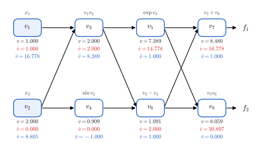
pp. 248–249 With a second output
\[ f_2(x_1,x_2)=(x_1x_2-\sin(x_2))\exp(x_1x_2), \tag{8.65} \]which is \(v_8=v_5v_6\) on the same trace (Figure 8.5), one forward pass gives both \(\partial f_1/\partial x_1\) and \(\partial f_2/\partial x_1\); the derivatives with respect to \(x_2\) need a second pass. In general one forward pass yields one column of the Jacobian
\[ \bJ=\begin{pmatrix}\frac{\partial f_1}{\partial x_1}&\cdots&\frac{\partial f_1}{\partial x_D}\\\vdots&\ddots&\vdots\\\frac{\partial f_K}{\partial x_1}&\cdots&\frac{\partial f_K}{\partial x_D}\end{pmatrix}, \tag{8.66} \]with seed \(\dot\bx=\be_i\), and the Jacobian-vector product
\[ \bJ\br=\begin{pmatrix}\frac{\partial f_1}{\partial x_1}&\cdots&\frac{\partial f_1}{\partial x_D}\\\vdots&\ddots&\vdots\\\frac{\partial f_K}{\partial x_1}&\cdots&\frac{\partial f_K}{\partial x_D}\end{pmatrix}\begin{pmatrix}r_1\\\vdots\\r_D\end{pmatrix} \tag{8.67} \]with seed \(\dot\bx=\br\). Forward mode suits few inputs and many outputs (\(K\gg D\)); training is the opposite case, one error and up to billions of weights, where forward mode would need one pass per weight.
8.2.2 Reverse-mode automatic differentiation
See also the companion course, Section 5.4.6 (fast multiplication by the Hessian).
pp. 249–250 Reverse mode generalises backpropagation. Each intermediate variable gets an adjoint
\[ \bar v_i=\frac{\partial f}{\partial v_i}, \tag{8.68} \]computed from the output backwards by the chain rule over the children \(\ch(i)\) (the nodes that use \(v_i\)):
\[ \bar v_i=\frac{\partial f}{\partial v_i}=\sum_{j\in\ch(i)}\frac{\partial f}{\partial v_j}\frac{\partial v_j}{\partial v_i}=\sum_{j\in\ch(i)}\bar v_j\frac{\partial v_j}{\partial v_i}. \tag{8.69} \]For the trace (8.50)–(8.56) this gives (Exercise 8.16)
\[ \bar v_7=1, \tag{8.70} \] \[ \bar v_6=\bar v_7, \tag{8.71} \] \[ \bar v_5=\bar v_7, \tag{8.72} \] \[ \bar v_4=-\bar v_6, \tag{8.73} \] \[ \bar v_3=\bar v_5v_5+\bar v_6, \tag{8.74} \] \[ \bar v_2=\bar v_3v_1+\bar v_4\cos(v_2), \tag{8.75} \] \[ \bar v_1=\bar v_3v_2. \tag{8.76} \]Erratum. (8.75) is printed as \(\bar v_2=\bar v_2v_1+\bar v_4\cos(v_2)\). The children of \(v_2\) are \(v_3=v_1v_2\) and \(v_4=\sin v_2\), so the first term is \(\bar v_3\,\partial v_3/\partial v_2=\bar v_3v_1\). As printed, the equation would force \(\bar v_4\cos v_2=0\) (with \(v_1=1\)), whereas at \((1,2)\) \(\bar v_4\cos v_2=0.416\); the corrected form gives \(\bar v_2=e^2+1-\cos2=\partial f/\partial x_2\) (checked). The solutions manual has the correct term.
One backward pass gives the derivatives with respect to all inputs; for a network error, all weight derivatives at once. With several outputs, one backward pass is needed per output. Reverse mode needs more memory, since every primal value must be stored for the backward pass, whereas forward mode can discard values as soon as they are used, which also makes it easier to implement. For both modes one pass costs at most a small constant times a function evaluation (the book quotes at most 6, typically 2 to 3; Griewank and Walther, 2008).
Result 8.9 (reverse mode: correctness, vector-Jacobian products, and backpropagation as a special case) pp. 249–250, (8.68)–(8.76); Exercise 8.16
(a) Process the nodes in reverse topological order, with the seed \(\bar f=1\) at the output. Then each \(\bar v_i\) from (8.69) equals the derivative of the output with respect to \(v_i\) when \(v_i\) is perturbed and everything computed from it is recomputed (all nodes not depending on \(v_i\) held fixed).
(b) Seeding the outputs with a vector \(\bu\) (\(\bar f_k=u_k\)) gives \(\bar x_j=(\bu^\T\bJ)_j\) at the inputs: a row of \(\bJ\) per pass with \(\bu=\be_k\), the whole gradient of a scalar in one pass.
(c) Applied to the trace of a network's error, the adjoint of each pre-activation is \(\bar a_j=\delta_j\) and the adjoint of each weight is \(\bar w_{ji}=\delta_jz_i\): Algorithm 8.1 is reverse mode on the error.
(d) Cost: one forward sweep that stores the \(n\) primal values, and one backward sweep with one multiply-add per edge (\(2e\) operations) plus the local partials, which reuse stored values. Memory: \(O(n)\).
Proof
(a) Reverse induction. For the output, \(\bar f=1\) is the derivative of \(f\) with respect to itself. Take node \(i\) and suppose the claim holds for every later node, in particular for its children. Perturbing \(v_i\) changes the output only through the values of its children (every other use of \(v_i\) is through a child), and each child \(v_j=\phi_j(\ldots,v_i,\ldots)\) changes by \((\partial\phi_j/\partial v_i)\,\d v_i\) to first order. By the chain rule and the induction hypothesis the output changes by \(\sum_{j\in\ch(i)}\bar v_j(\partial v_j/\partial v_i)\,\d v_i\), which is (8.69). The order is legitimate because all children of \(i\) come after \(i\). Applying (8.69) to Figure 8.4 node by node gives (8.70)–(8.76) (Exercise 8.16).
(b) The recursion is linear in the seeds, so seeding \(u_k\) on output \(k\) yields \(\sum_ku_k\,\partial f_k/\partial x_j\).
(c) In the network trace, \(a_j\) has the children \(z_j=h(a_j)\) only, with local derivative \(h'(a_j)\), and \(z_j\) has the children \(a_k\), \(k\in\ch(j)\), with local derivatives \(w_{kj}\). So \(\bar z_j=\sum_kw_{kj}\bar a_k\) and \(\bar a_j=h'(a_j)\bar z_j\), which is (8.13) with \(\bar a=\delta\); at the outputs \(\bar a_k=\partial E_n/\partial a_k=\delta_k\). A weight \(w_{ji}\) has the single child \(a_j\) with local derivative \(z_i\): \(\bar w_{ji}=\delta_jz_i\), which is (8.10). Checked on the worked example: the tape's adjoints equal the deltas and the gradient to \(10^{-15}\).
(d) Each edge \(i\to j\) contributes one product \(\bar v_j\cdot\partial v_j/\partial v_i\) and one addition. The local partials of the elementary operations are functions of the stored values (for \(v_3=v_1v_2\), they are \(v_2\) and \(v_1\); for \(v_5=e^{v_3}\), the stored \(v_5\) itself), which is why the values must be kept.
Filling the gap 8.9: the memory of reverse mode, and checkpointing p. 250
Derivation
For a network of \(L\) layers trained on a mini-batch of \(B\) points, reverse mode keeps every layer's pre-activations (or activations) for the whole batch until the backward sweep reaches that layer: memory \(O(B\sum_lM_l)\), usually far more than the weights themselves. Forward mode needs only the current layer, but would need one pass per weight.
Checkpointing trades time for memory. Store the activations only at every \(k\)-th layer (the checkpoints) during the forward sweep. During the backward sweep, when a segment of \(k\) layers is reached, recompute its activations from the checkpoint below it, use them, and discard them. Memory: \(L/k\) checkpoints plus one segment of \(k\) layers, minimised at \(k\approx\sqrt L\), giving \(O(\sqrt L)\) layers in memory instead of \(O(L)\). Time: every layer is recomputed at most once, so the cost rises by at most one forward pass, about a third more work than plain backpropagation (Result 8.2). Recursive schemes reduce memory to \(O(\log L)\) at a cost of \(O(\log L)\) recomputations per layer (Griewank and Walther, 2008).
p. 250 Hybrids of the two modes are useful too. For the product of the Hessian with a vector \(\bv\) at a point \(\bx\) (Pearlmutter, 1994): forward mode with \(\dot\bx=\bv\) gives the directional derivative \(\bv^\T\nabla f\), and reverse mode applied to that code gives \(\nabla^2f\,\bv=\bH\bv\), at cost \(O(W)\) although \(\bH\) is \(W\times W\). The full Hessian by automatic differentiation costs \(O(W^2)\).
Erratum. The text starts "from a vector \(\bb\) and a point \(\bx\)" and then uses \(\bv\); the vector is \(\bv\) throughout.
Result 8.10 (Hessian-vector products by nesting the two modes) p. 250
Let \(f\) be twice continuously differentiable. (a) Reverse over forward (the book's order): run forward mode with \(\dot\bx=\bv\) to obtain the program for \(g(\bx)=\bv^\T\nabla f(\bx)\); reverse mode on it gives \(\nabla g=\bH\bv\). (b) Forward over reverse: run reverse mode on inputs that carry the tangent \(\bv\) (each value a dual number); the tangent parts of the adjoints \(\bar\bx\) are \(\bH\bv\). Both cost a constant multiple of evaluating \(f\), \(O(W)\) for a network; the full Hessian takes \(W\) such products, \(O(W^2)\).
Proof
(a) \(g(\bx)=\sum_jv_j\,\partial f/\partial x_j\) with \(\bv\) constant, so \(\partial g/\partial x_i=\sum_jv_j\,\partial^2f/\partial x_i\partial x_j=(\bH\bv)_i\) (\(\bH\) is symmetric by Schwarz's theorem, since \(f\in C^2\)). By Result 8.8(a) the forward-mode program computes \(g\) exactly as a trace of elementary operations, and by Result 8.9(b) reverse mode returns its gradient. (b) Reverse mode computes \(\nabla f(\bx)\) through a program of elementary operations; running that program on \(\bx+\bv\varepsilon\) gives, by Result 8.8(a), \(\nabla f(\bx)+\varepsilon\,\frac{\d}{\d r}\nabla f(\bx+r\bv)|_{r=0}=\nabla f+\varepsilon\bH\bv\). Each nesting multiplies the cost by a constant, so the total is a constant times one evaluation of \(f\). This is the R-operator of Result 8.7 generated automatically. Checked: both orders, built from the code's own Dual and Var classes, agree with autograd's Hessian-vector product to \(10^{-13}\), and \(W\) products reproduce the full Hessian.
Filling the gap 8.10: why one pass costs only a constant times one evaluation p. 250
Derivation
Measure cost in elementary operations, each with at most two arguments. A trace with \(n\) operations has \(e\le2n\) edges. Forward mode adds, per operation, at most one derivative evaluation and one multiply-add per argument: at most \(n+2e\le5n\) operations including the primal ones, plus derivative evaluations. Reverse mode records the \(n\) primal operations and then, per edge, one multiplication by a stored local partial and one addition: \(n+2e\) again, plus the local partials. Neither count depends on the number of inputs or weights: that is the "cheap gradient principle" behind the book's bound (Griewank and Walther, 2008, prove a bound of this kind under a precise cost model; the exact constant depends on what is counted, memory traffic included). In the networks of Figure 8.S1, \(e/n\le1.49\), and backpropagation took 2.87 forward passes' worth of multiply-adds (checked), in line with the "factor of 2 or 3" quoted by the book.
Summary: errors and imprecisions found in the chapter (first printing) and in the solutions manual
- p. 248: the derivative \(\partial f/\partial x_1\) is \(\dot v_7\), not "\(\dot v_5\)" (at \((1,2)\): 16.78 against 14.78; checked).
- (8.75): \(\bar v_2=\bar v_3v_1+\bar v_4\cos v_2\), not \(\bar v_2v_1+\ldots\) (as printed the equation is self-referential and inconsistent at \((1,2)\); checked). The manual's Solution 8.16 has it right.
- p. 250: "a vector \(\bb\)" should be \(\bv\).
- (8.44)–(8.47): written with \(h\) although the soft ReLU is named \(\zeta\) in (8.46) (notation only).
- Section 8.1.6 and Exercise 8.9 (imprecision): the averaging argument and (8.79) need the network to be able to represent the regression function; with systematic residuals the dropped term does not vanish as \(N\) grows (Filling the gap 8.6, Figure 8.S2(b)).
- Exercise 8.12 (imprecision): the one-pass inverse is insensitive to \(\alpha\) only if \(\alpha\ll\lambda_{\min}(\HOP)\), and if \(NK<W\) it depends on \(\alpha\) entirely (Filling the gap 8.7, Figure 8.S4).
- Manual, Solution 8.1: "the chain rule of probability" should be the chain rule of calculus.
- Manual, Solution 8.2, (263): \(\bW^{(l-1)\T}\) should be \(\bW^{(l)\T}\) (checked against autograd).
- Manual, Solution 8.5: the initial value of \(\partial a_j/\partial x_i\) is \(w_{ji}\), not \(w_{ij}\).
- Manual, Solution 8.6: in (275) \(h'(a_j)\) should be \(h'(a_{j'})\); "we obtain (??)" leaves the first-layer block unwritten; the final mixed-layer formula drops \(z_{j'}\) (and writes \(w^{(1)}_{ij}\) for \(w^{(1)}_{ji}\)); checked numerically.
- Manual, Solution 8.7: "Section ??" (a broken reference; the formulas are correct).
- Manual, Solution 8.10: \(\nabla a_n\nabla a_n\) lacks the transpose; Solution 8.12: \(\bb_{L+1}\) is used for \(\nabla a_{L+1}\) without definition.
Exercises
All 18 exercises of Chapter 8 (Bishop and Bishop, 2024, pp. 250–252), restated in my own words, with complete solutions (hidden). Stars give the book's difficulty. Each was solved independently and then compared with the official solutions manual; where they differ, the solution says so and why.
Exercise 8.1 (★). Use (8.5), (8.6), (8.8) and (8.12) to derive the backpropagation formula (8.13).
Solution
By (8.12), \(\delta_j=\sum_k\delta_k\,\partial a_k/\partial a_j\). By (8.5), \(a_k=\sum_{j'}w_{kj'}z_{j'}\), and by (8.6), \(z_{j'}=h(a_{j'})\); only the term \(j'=j\) depends on \(a_j\), so \(\partial a_k/\partial a_j=w_{kj}h'(a_j)\). Hence \(\delta_j=h'(a_j)\sum_kw_{kj}\delta_k\). (Result 8.1 also explains why the sum runs only over the children of \(j\). Same as the manual, which says "chain rule of probability" for the chain rule of calculus.)
Exercise 8.2 (★★). For a layered network with forward equations (6.19), write (8.13) in matrix form and observe that transposed weight matrices appear.
Solution
\(\bdelta^{(l-1)}=h'(\ba^{(l-1)})\odot(\bW^{(l)\T}\bdelta^{(l)})\), and \(\nabla_{\bW^{(l)}}E_n=\bdelta^{(l)}\bz^{(l-1)\T}\); for a mini-batch, \(\boldsymbol\Delta^{(l-1)}=h'(\mathbf{A}^{(l-1)})\odot(\boldsymbol\Delta^{(l)}\bW^{(l)})\) and \(\nabla_{\bW^{(l)}}E=\boldsymbol\Delta^{(l)\T}\mathbf{Z}^{(l-1)}\) (Filling the gap 8.2). The transpose appears because (8.5) sums over the second index of \(w_{kj}\) and (8.13) over the first. The manual writes \(\bW^{(l-1)\T}\), an index slip: the matrix is the one that maps layer \(l-1\) to layer \(l\), \(\bW^{(l)}\) (checked).
Exercise 8.3 (★). Show with a Taylor expansion that the \(O(\epsilon)\) terms cancel in the central difference (8.25).
Solution
\(E(w\pm\epsilon)=E\pm\epsilon E'+\tfrac12\epsilon^2E''\pm\tfrac16\epsilon^3E'''(\xi_\pm)\). In the difference the terms \(E\) and \(\tfrac12\epsilon^2E''\) cancel, leaving \(2\epsilon E'+O(\epsilon^3)\); dividing by \(2\epsilon\) gives \(E'+O(\epsilon^2)\), with error exactly \(\tfrac{\epsilon^2}{6}E'''(\xi)\) (Result 8.3). In the one-sided difference, the term \(\tfrac12\epsilon^2E''\) survives and gives the \(O(\epsilon)\) error. Same as the manual.
Exercise 8.4 (★★). Add skip-layer weights from the inputs directly to the outputs of the two-layer network of Figure 6.9 and find the derivatives of the error with respect to them.
Solution
Only (8.20) changes: \(y_k=\sum_{j=0}^Mw^{(2)}_{kj}z_j+\sum_{i=1}^Du_{ki}x_i\) (no separate skip bias is needed; the output bias already exists). The weight \(u_{ki}\) enters only \(a_k\), with \(\partial a_k/\partial u_{ki}=x_i\), so \(\partial E_n/\partial u_{ki}=\delta_kx_i\), using the output errors (8.21) already computed. Nothing else in (8.21)–(8.23) changes, because the hidden units do not see the skip weights. Checked against central differences for linear and softmax outputs; demo preset 4. Same as the manual.
Exercise 8.5 (★★★). Derive a forward-propagation method for the Jacobian, as an alternative to the backward method of Section 8.1.5.
Solution
Propagate \(G_{ji}=\partial a_j/\partial x_i\) forwards with the activations: \(G_{ji}=w_{ji}\) for units fed by the inputs, and \(G_{li}=\sum_jw_{lj}h'(a_j)G_{ji}\) in topological order; finally \(J_{ki}=\sum_l(\partial y_k/\partial a_l)G_{li}\) with (8.31), (8.33) or (8.34). In matrix form this evaluates \(\bS^{(L)}\bW^{(L)}\cdots\bS^{(1)}\bW^{(1)}\) from the right. Each column \(i\) costs one forward pass, \(O(DW)\) in all; the backward method costs \(O(KW)\), so the forward one is preferable when \(D<K\) (Result 8.4; checked against autograd). Same as the manual, which writes the initial value as \(w_{ij}\) for \(w_{ji}\).
Exercise 8.6 (★★★). For a two-layer network, with \(\delta_k=\partial E_n/\partial a_k\) and \(M_{kk'}=\partial^2E_n/\partial a_k\partial a_{k'}\) (8.77), express the Hessian when (i) both weights are in the second layer, (ii) both in the first layer, (iii) one in each.
Solution
(i) \(z_jz_{j'}M_{kk'}\). (ii) \(x_ix_{i'}\big[h''(a_j)I_{jj'}\sum_kw^{(2)}_{kj}\delta_k+h'(a_j)h'(a_{j'})\sum_{k,k'}w^{(2)}_{kj}w^{(2)}_{k'j'}M_{kk'}\big]\). (iii) \(x_ih'(a_j)\big[\delta_kI_{jj'}+z_{j'}\sum_{k'}w^{(2)}_{k'j}M_{kk'}\big]\). The derivation is in Result 8.6; the assembled Hessian equals autograd's to \(10^{-11}\). The manual's route is the same, but its (275) has \(h'(a_j)\) where \(h'(a_{j'})\) belongs, its result for (ii) is a broken reference "(??)", and its final formula for (iii) omits \(z_{j'}\) (a wrong value, checked).
Exercise 8.7 (★★★). Extend Exercise 8.6 to a network with skip-layer weights from the inputs to the outputs.
Solution
Three new blocks: \(\partial^2E_n/\partial u_{ki}\partial u_{k'i'}=M_{kk'}x_ix_{i'}\), \(\partial^2E_n/\partial u_{ki}\partial w^{(2)}_{k'j}=M_{kk'}z_jx_i\), and \(\partial^2E_n/\partial u_{ki}\partial w^{(1)}_{ji'}=x_ix_{i'}h'(a_j)\sum_{k'}M_{kk'}w^{(2)}_{k'j}\); the three blocks of Exercise 8.6 are unchanged because the skip weights enter only the output pre-activations. Proof in Result 8.6; checked for linear, logistic and softmax outputs. Same as the manual.
Exercise 8.8 (★★). Extend the outer-product approximation (8.40) to a network with several outputs and the sum-of-squares error.
Solution
With \(E=\frac12\sum_n\|\by_n-\bt_n\|^2\), \(\bH=\sum_n\sum_k\nabla y_{nk}\nabla y_{nk}^\T+\sum_n\sum_k(y_{nk}-t_{nk})\nabla\nabla y_{nk}\), so \(\bH\simeq\sum_n\bB_n^\T\bB_n\) with \(\bB_n=\partial\by_n/\partial\bw\) (\(K\times W\)), a sum of \(NK\) outer products (Result 8.5 with \(\bM_n=\bI\); exact when the residuals vanish, checked). Same as the manual, which arranges \(\bB_n\) as \(W\times K\).
Exercise 8.9 (★★). For \(E(\bw)=\frac12\iint\{y(\bx,\bw)-t\}^2p(\bx,t)\,\d\bx\,\d t\) (8.78), use the fact that the minimising function is \(\E[t\given\bx]\) (4.37) to show that the second derivatives are \(\int(\partial y/\partial w_r)(\partial y/\partial w_s)p(\bx)\,\d\bx\) (8.79), and relate this to (8.40).
Solution
Differentiating twice and integrating over \(t\) first, \(\partial^2E/\partial w_r\partial w_s=\int\partial_ry\,\partial_sy\,p(\bx)\,\d\bx+\int(y-\E[t\given\bx])\,\partial_r\partial_sy\,p(\bx)\,\d\bx\). At weights where \(y(\bx,\bw)=\E[t\given\bx]\) the second integral vanishes, which is (8.79). Replacing the integral by an average over a sample \(\bx_1,\ldots,\bx_N\) from \(p(\bx)\) gives \(\frac1N\sum_n\nabla y_n\nabla y_n^\T\), the outer product (8.40) up to the factor \(1/N\) (from using an average rather than a sum). The step "the minimiser is \(\E[t\given\bx]\)" assumes the network can represent it; otherwise the second integral is \(\int b(\bx)\partial_r\partial_sy\,p\,\d\bx\) with the bias \(b\), which need not vanish (Filling the gap 8.6). Same as the manual, which makes that assumption silently.
Exercise 8.10 (★★). Derive the outer-product approximation (8.41) for one logistic-sigmoid output and the cross-entropy error.
Solution
For \(E=-\sum_n[t_n\ln y_n+(1-t_n)\ln(1-y_n)]\) with \(y_n=\sigma(a_n)\), \(\partial E/\partial a_n=y_n-t_n\), so \(\nabla E=\sum_n(y_n-t_n)\nabla a_n\). Differentiating again, with \(\partial y_n/\partial a_n=y_n(1-y_n)\), \(\nabla\nabla E=\sum_ny_n(1-y_n)\nabla a_n\nabla a_n^\T+\sum_n(y_n-t_n)\nabla\nabla a_n\); dropping the second sum gives (8.41). It is exact when \(y_n=t_n\) (checked) and always positive semi-definite. Same as the manual (which omits a transpose).
Exercise 8.11 (★★). Derive the outer-product approximation for \(K\) softmax outputs with the cross-entropy error.
Solution
\(\partial E/\partial a_{nk}=y_{nk}-t_{nk}\) and \(\partial y_{nk}/\partial a_{nl}=y_{nk}(I_{kl}-y_{nl})\) (8.34), so \(\bH=\sum_n\sum_{k,l}y_{nk}(I_{kl}-y_{nl})\nabla a_{nk}\nabla a_{nl}^\T+\sum_n\sum_k(y_{nk}-t_{nk})\nabla\nabla a_{nk}\), and \(\bH\simeq\sum_n\bB_n^\T(\diag\by_n-\by_n\by_n^\T)\bB_n\). The middle matrix is a covariance matrix, so the approximation is positive semi-definite; it equals autograd's Hessian when the targets equal the outputs (checked). Same as the manual.
Exercise 8.12 (★★★). Apply the rank-one identity (8.80) to the outer-product approximation to obtain a one-pass algorithm for the inverse Hessian, started from \(\bH=\alpha\bI\).
Solution
\(\bH_{L+1}=\bH_L+\bb_{L+1}\bb_{L+1}^\T\) with \(\bb_{L+1}=\nabla a_{L+1}\), so by (8.80) \(\bH_{L+1}^{-1}=\bH_L^{-1}-(\bH_L^{-1}\bb_{L+1})(\bH_L^{-1}\bb_{L+1})^\T/(1+\bb_{L+1}^\T\bH_L^{-1}\bb_{L+1})\), \(O(W^2)\) per point (Algorithm 8.2). The result is exactly \((\HOP+\alpha\bI)^{-1}\), and is close to \(\HOP^{-1}\) only if \(\alpha\ll\lambda_{\min}(\HOP)\) (Filling the gap 8.7; the exercise's "not particularly sensitive" needs this qualification). Same algorithm as the manual.
Exercise 8.13 (★★). Verify that differentiating (8.47) with respect to \(w_1\) gives (8.48).
Solution
\(\zeta'(a)=e^a/(1+e^a)=\sigma(a)\). With \(z=\zeta(w_1x+b_1)\), \(\partial z/\partial w_1=x\,e^{w_1x+b_1}/(1+e^{w_1x+b_1})\) and \(\partial y/\partial z=w_2\,e^{w_2z+b_2}/(1+e^{w_2z+b_2})\). Multiply, substitute \(z=\ln(1+e^{w_1x+b_1})\), and combine \(e^{w_1x+b_1}e^{w_2z+b_2}=\exp(w_1x+b_1+b_2+w_2\ln[1+e^{w_1x+b_1}])\): this is (8.48). Checked against reverse mode at two points. Same as the manual.
Exercise 8.14 (★★). For the logistic map \(L_{n+1}=4L_n(1-L_n)\), \(L_1=x\), write the evaluation traces of \(L_2,L_3,L_4\) and, without simplifying, the derivatives \(L_1',\ldots,L_4'\); compare how fast the expressions grow.
Solution
Trace: \(v_1=x\), and for each step \(u=1-L\), \(p=L\cdot u\), \(L_{\rm new}=4p\): three operations per step. Functions: \(L_2=4x(1-x)\), \(L_3=16x(1-x)(1-2x)^2\), \(L_4=64x(1-x)(1-2x)^2(1-8x+8x^2)^2\) (using \(1-L_3=(1-8x+8x^2)^2\)). Derivatives by the product rule, unsimplified: \(L_1'=1\), \(L_2'=4(1-x)-4x\), \(L_3'=16(1-x)(1-2x)^2-16x(1-2x)^2-64x(1-x)(1-2x)\), and \[L_4'=64(1-x)(1-2x)^2q^2-64x(1-2x)^2q^2-256x(1-x)(1-2x)q^2+128x(1-x)(1-2x)^2q(16x-8),\] with \(q=1-8x+8x^2\). Each derivative has more terms than the one before, roughly doubling, while each new function adds one factor; written out without sharing the counts are exact: \(s_n=6\cdot2^{n-1}-5\) and \(d_n=(6n-8)2^n+5\) (Filling the gap 8.8). The forward-mode trace grows by a fixed number of operations per step. Checked: \(L_4'(0.3)=1.3090816\) from the formula, the manual's (308) and forward mode. Same as the manual.
Exercise 8.15 (★★). Derive the tangent equations (8.58)–(8.64) from the trace (8.50)–(8.56) using (8.57).
Solution
Seeds \(\dot v_1=1\), \(\dot v_2=0\) for \(\partial/\partial x_1\). Then \(\dot v_3=\dot v_1\,\partial v_3/\partial v_1+\dot v_2\,\partial v_3/\partial v_2=\dot v_1v_2+\dot v_2v_1\); \(\dot v_4=\dot v_2\cos v_2\); \(\dot v_5=\dot v_3e^{v_3}\); \(\dot v_6=\dot v_3-\dot v_4\); \(\dot v_7=\dot v_5+\dot v_6\), using the parents shown in Figure 8.4. Same as the manual.
Exercise 8.16 (★★). Derive the adjoint equations (8.70)–(8.76) from the trace and Figure 8.4 using (8.69).
Solution
Children: \(\ch(7)=\varnothing\), \(\ch(6)=\ch(5)=\{7\}\), \(\ch(4)=\{6\}\), \(\ch(3)=\{5,6\}\), \(\ch(2)=\{3,4\}\), \(\ch(1)=\{3\}\). So \(\bar v_7=1\); \(\bar v_6=\bar v_7\cdot1\); \(\bar v_5=\bar v_7\cdot1\); \(\bar v_4=\bar v_6\cdot(-1)\); \(\bar v_3=\bar v_5e^{v_3}+\bar v_6=\bar v_5v_5+\bar v_6\); \(\bar v_2=\bar v_3v_1+\bar v_4\cos v_2\); \(\bar v_1=\bar v_3v_2\). The first term of \(\bar v_2\) is \(\bar v_3v_1\), not \(\bar v_2v_1\) as printed in (8.75) (see the erratum). Same as the manual.
Exercise 8.17 (★★★). Find \(\partial f/\partial x_1\) for (8.49) and evaluate it at \((1,2)\); then evaluate the primal, tangent and adjoint traces at that point and confirm that both modes give the same value.
Solution
\(\partial f/\partial x_1=x_2+x_2e^{x_1x_2}=2+2e^2=16.7781\). Primal: \(v_1=1\), \(v_2=2\), \(v_3=2\), \(v_4=\sin2=0.9093\), \(v_5=e^2=7.3891\), \(v_6=2-\sin2=1.0907\), \(v_7=2+e^2-\sin2=8.4798\). Tangents: \(1,0,2,0,2e^2,2,2+2e^2\), so \(\dot v_7=16.7781\). Adjoints: \(\bar v_7=\bar v_6=\bar v_5=1\), \(\bar v_4=-1\), \(\bar v_3=e^2+1=8.3891\), \(\bar v_2=e^2+1-\cos2=8.8052\), \(\bar v_1=2e^2+2=16.7781\). Both agree with the direct value, and reverse mode gives \(\partial f/\partial x_2=x_1+x_1e^{x_1x_2}-\cos x_2\) in the same pass (Figure 8.4; checked to \(10^{-15}\); demo preset 1). Same as the manual.
Exercise 8.18 (★★). Writing \(\br=\sum_ir_i\be_i\), show that \(\bJ\br\) (8.67) is obtained by one forward-mode pass with \(\dot\bx=\br\).
Solution
The tangent recursion (8.57) is linear in the seed, so the output tangents for \(\dot\bx=\sum_ir_i\be_i\) are \(\sum_ir_i\) times those for \(\be_i\), i.e. \(\sum_ir_i\bJ\be_i=\bJ\br\). Equivalently, \(\bx(s)=\bx+s\br\) is a one-input function whose Jacobian with respect to \(s\) is the single column \(\bJ\br\), and forward mode with \(\dot s=1\) induces \(\dot\bx=\br\) (Result 8.8(b); checked). Same as the manual.
Demonstrations
Three interactive pages, each linked above where its topic arises. They run in the browser and reproduce the Python code number for number (relative differences at most \(2.2\times10^{-16}\)).
- Backpropagation step by step, with a gradient check: Algorithm 8.1 stage by stage on a two-layer network (tanh, logistic or ReLU hidden units; linear, logistic or softmax outputs; optional skip weights), and the error of finite and central differences against \(\epsilon\) for any weight. Presets: 1 step by step, 2 Figure 8.2 live, 3 softmax outputs, 4 skip weights, 5 a ReLU at its kink.
- Forward mode and reverse mode on an evaluation trace: the traces of (8.49), Figure 8.5, the soft-ReLU network (8.47) and the logistic map, with tangents, adjoints, local derivatives on the edges and the cost of the full Jacobian. Presets: 1 forward mode (Exercise 8.17), 2 reverse mode, 3 two outputs, 4 a network, 5 expression swell.
- The Hessian, the outer-product approximation and Hessian-vector products: a 1-\(M\)-1 network trained live, its exact Hessian and \(\HOP\) as heat maps and eigenvalues, the error of the approximation during training, and \(\bH\bv\) by the R-operator and by finite differences. Presets: 1 initialisation, 2 trained, noise-free, 3 noisy targets, 4 too few hidden units, 5 Hessian-vector products.
References
- Bishop, C. M. and Bishop, H. (2024). Deep Learning: Foundations and Concepts. Springer, Cham. Chapter 8, pp. 233–252. doi:10.1007/978-3-031-45468-4. Book website: www.bishopbook.com.
- Bishop, C. M. and Bishop, H. (2024). Deep Learning: Foundations and Concepts, Solutions to Exercises, version 1.0 (Chapters 2–10).
- Baydin, A. G., Pearlmutter, B. A., Radul, A. A. and Siskind, J. M. (2018). Automatic differentiation in machine learning: a survey. Journal of Machine Learning Research, 18(153), 1–43.
- Becker, S. and LeCun, Y. (1989). Improving the convergence of back-propagation learning with second order methods. In Proceedings of the 1988 Connectionist Models Summer School, 29–37. Morgan Kaufmann.
- Bishop, C. M. (1992). Exact calculation of the Hessian matrix for the multilayer perceptron. Neural Computation, 4(4), 494–501.
- Bishop, C. M. (2006). Pattern Recognition and Machine Learning. Springer.
- Griewank, A. and Walther, A. (2008). Evaluating Derivatives: Principles and Techniques of Algorithmic Differentiation, 2nd edition. SIAM.
- Hassibi, B. and Stork, D. G. (1993). Second order derivatives for network pruning: Optimal Brain Surgeon. In Advances in Neural Information Processing Systems 5, 164–171.
- LeCun, Y., Denker, J. S. and Solla, S. A. (1990). Optimal brain damage. In Advances in Neural Information Processing Systems 2, 598–605.
- MacKay, D. J. C. (1992). A practical Bayesian framework for back-propagation networks. Neural Computation, 4(3), 448–472.
- Møller, M. (1993). Exact calculation of the product of the Hessian matrix of feed-forward network error functions and a vector in O(N) time. Technical report DAIMI PB-432, Aarhus University.
- Pearlmutter, B. A. (1994). Fast exact multiplication by the Hessian. Neural Computation, 6(1), 147–160.
- Ricotti, L. P., Ragazzini, S. and Martinelli, G. (1988). Learning of word stress in a sub-optimal second order back-propagation neural network. In Proceedings of the IEEE International Conference on Neural Networks, volume 1, 355–361.
- Shen, S., Dong, Z., Ye, J., Ma, L., Yao, Z., Gholami, A., Mahoney, M. W. and Keutzer, K. (2019). Q-BERT: Hessian based ultra low precision quantization of BERT. arXiv:1909.05840.
Every numerical statement in these notes comes from ch08_backpropagation.py.