Introduction
The book's first chapter is two pages: it argues for a model-based approach to machine learning (learn a parsimonious model of the data-generating process, so that systems are robust to change and learn from little data), separates Bayesian inference, which inverts a function, from the deep-learning use of the word, which evaluates one, and lays out the four kinds of task (prediction, generation, discovery, control) that organise the six Parts. These notes expand the map into a guide to the whole course, with links to the chapter that develops each Part and to the companion courses, and make the remark about inversion precise on a small example.
Ch. 1 Introduction Ch. 2 Probability Ch. 3 Statistics Ch. 4 Graphical models Ch. 5 Information theory Ch. 6 Optimisation Ch. 7 Inference algorithms Ch. 8 Gaussian filtering Ch. 9 Message passing Ch. 10 Variational inference Ch. 11 Monte Carlo Ch. 12 MCMC Ch. 13 Sequential Monte Carlo Ch. 14 Predictive models Ch. 15 GLMs Ch. 16 Deep networks Ch. 17 Bayesian neural networks Ch. 18 Gaussian processes Ch. 19 Beyond iid Ch. 20 Generative models Ch. 21 VAEs Ch. 22 Autoregressive models Ch. 23 Normalizing flows Ch. 24 Energy-based models Ch. 25 Diffusion models Ch. 26 GANs Ch. 27 Discovery methods Ch. 28 Latent factor models Ch. 29 State-space models Ch. 30 Graph learning Ch. 31 Nonparametric Bayes Ch. 32 Representation learning Ch. 33 Interpretability Ch. 34 Decision making Ch. 35 Reinforcement learning Ch. 36 Causality
How to read these notes
They follow the book. The book's Chapter 1 has no numbered sections and no equations; it is a two-page statement of aims and a map of the book. I label its parts 1.1 to 1.3 for navigation (these are my labels, not the book's). The notes expand the map into a guide to the whole course: each Part is a row of the table in Section 1.3, with links to the chapters of this course that develop it.
Filling the gaps. The chapter makes one technical remark, that Bayesian inference "inverts a function" and is a harder task than evaluating it; an orange Filling the gap box makes this precise on a tiny example. Proofs start hidden.
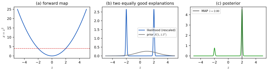
Figures. The chapter has no figure. One figure of my own illustrates the remark on inversion.
Main reference
K. P. Murphy, Probabilistic Machine Learning: Advanced Topics, MIT Press (2023; December 2025 draft), Chapter 1, pages 1–2 (book page: probml.github.io/pml-book/book2.html). The explanations, derivations, figure and code are my own.
Companion courses
- Probabilistic Machine Learning: An Introduction (Murphy's first volume, the prequel to this one): Chapter 1 introduction and the whole course home.
- Bayesian and Probabilistic Machine Learning (Bishop): Chapter 1.
- Foundations of Deep Learning (Bishop and Bishop): Chapter 1; Introduction to Statistical Learning: Chapter 1; All of Statistics: Chapter 1 and Chapter 6 (models, statistical inference and learning).
1.1 Why a model-based approach
p. 1 Much of current machine learning is about mapping inputs to outputs, \(f:\mathcal X\to\mathcal Y\), often with deep networks. Judea Pearl called this "glorified curve fitting"; the book finds that a little unfair, since for high-dimensional \(\mathcal X\) or \(\mathcal Y\) (images, sentences, graphs, sequences of actions) one-dimensional intuitions about curve fitting fail, but it agrees with what the quote points at: such methods concentrate on predicting observable patterns and not on understanding the latent structure behind them. Understanding of that kind matters for science and for applications such as healthcare, where the aim is to find the mechanism of a disease, and it is needed to build systems that are
- robust: they keep working when the data distribution changes unexpectedly (robotics is the standard example; see Chapter 19 on distribution shift);
- efficient, chiefly statistically efficient: they learn from small samples, which matters where data are scarce (healthcare, robotics) even though they are abundant for language and vision. Computational efficiency is a secondary concern.
The book's answer is a model-based approach: learn a parsimonious representation of the unknown data-generating process (DGP) from samples of one or more data sets, much as science proceeds by explaining observations with theories or models. One way to formalise this is Bayesian inference applied to probabilistic models. Part II of the book is about inference algorithms (the overview is Chapter 7); Part I collects background that a reader who knows probability, statistics, graphical models, information theory and optimisation can skip: Chapter 2 (probability), 3 (statistics), 4 (graphical models), 5 (information theory), 6 (optimisation).
1.2 Inference is inversion
p. 1, footnote 1 The word "inference" is used in two ways. In the deep-learning community it means applying a function to inputs to get outputs (the forward pass of a trained network). In Bayesian statistics it means inverting a function: from observed outputs, work backwards to the hidden inputs (causes) that could have produced them, which is a much harder task, and is closer to what the deep-learning community calls "training". The footnote's point is easiest to see when the forward map is many-to-one.
Filling the gap 1.1: why inversion needs a prior, on a small example p. 1, footnote 1
Derivation
Let a hidden scalar \(z\) produce an observation \(x=f(z)+\varepsilon\) with Gaussian noise \(\varepsilon\sim\mathcal N(0,\sigma^2)\), where \(f(z)=z^2\) (a many-to-one map: \(z\) and \(-z\) give the same \(x\)). Evaluating the forward map is trivial. To invert it, apply Bayes' rule with a prior \(p(z)\): \[ p(z\given x)=\frac{p(x\given z)\,p(z)}{\int p(x\given z')p(z')\,\d z'},\qquad p(x\given z)=\mathcal N(x\given z^2,\sigma^2). \] Because \(p(x\given z)=p(x\given-z)\), the likelihood has two exactly equal peaks at \(z=\pm\sqrt x\) (for \(x>0\), small \(\sigma\)), and so the likelihood alone cannot tell which cause produced the data: it is not even maximised at a unique point. What decides is the prior. Dividing the posterior at \(z\) by that at \(-z\), the equal likelihoods and the common denominator cancel: \[ \frac{p(z\given x)}{p(-z\given x)}=\frac{p(z)}{p(-z)}. \] So the evidence in the data about the sign is exactly nil, and the posterior odds of the two explanations are the prior odds. With the prior \(\mathcal N(1,1.5^2)\), \(x=4\) (so \(z=\pm2\)) the ratio is \(\exp\big(\frac{(-2-1)^2-(2-1)^2}{2\cdot1.5^2}\big)=e^{8/4.5}=5.92\): the explanation \(z=+2\) is about six times as probable as \(z=-2\), and the MAP estimate \(\hat z=\argmax p(z)p(x\given z)\) of equation (27.1) in Chapter 27 lies near \(+2\) (the own figure below; the ratio and the symmetry were confirmed on a grid). With a symmetric prior such as \(\mathcal N(0,\tau^2)\) the ratio is 1 and the posterior is exactly symmetric: it has two modes of equal height and a mean of 0 that is not a plausible cause at all (since \(z=0\) predicts \(x=0\), not 4). Forward evaluation was a function; inversion is a distribution, and a prior is what makes it well defined.
1.3 Four kinds of task and the plan of the book
p. 2 The right model depends on the task, the kind and amount of data and the metric of success. The book considers four kinds of task: prediction (classification and regression), generation (of images or text), discovery (of meaningful structure in data) and control (optimal decision making). The six Parts follow:
| Part | Subject | Chapters in this course | Companion courses |
|---|---|---|---|
| I Fundamentals | background that can be skipped by readers who know it | 2 probability, 3 statistics, 4 graphical models, 5 information theory, 6 optimisation | Introduction volume Chapters 2–8; All of Statistics; Bayesian and Probabilistic ML Chapters 1–2 |
| II Inference | computing posteriors: exact, Gaussian, message passing, variational, Monte Carlo | 7 overview, 8 Gaussian filtering and smoothing, 9 message passing, 10 variational inference, 11 Monte Carlo, 12 MCMC, 13 sequential Monte Carlo | ML 10, ML 11, AoS 24 |
| III Prediction | conditional models \(p(y\given x)\): one right answer, possibly uncertain | 14 overview, 15 GLMs, 16 deep networks, 17 Bayesian networks, 18 Gaussian processes, 19 beyond i.i.d. | PML 10–13, 17, Deep Learning, ISL |
| IV Generation | distributions \(p(x)\) or \(p(x\given c)\) with several valid outputs; harder to evaluate | 20 overview, 21 VAEs, 22 autoregressive, 23 flows, 24 energy-based, 25 diffusion, 26 GANs | DL 16–20 |
| V Discovery | latent-variable models \(p(z)p(x\given z)\) and the computation of \(p(z\given x)\); interpretation of predictive models | 27 overview, 28 latent factors, 29 state-space, 30 graphs, 31 nonparametric Bayes, 32 representations, 33 interpretability | PML 20–21, ML 12–13, NPS 10 |
| VI Decisions | decisions under uncertainty, ending with causality | 34 decision making, 35 reinforcement learning, 36 causality | PML 5, AoS 16 |
Prediction (Part III). Models \(p(y\given x)\) with a high-dimensional input \(x\in\mathcal X\) and low-dimensional output \(y\in\mathcal Y\); there is one right answer, though we may be uncertain about it. Generation (Part IV). Models \(p(x)\) or \(p(x\given c)\) for a conditioning input \(c\) such as a text prompt: many outputs match the prompt, so evaluation is harder than for prediction since the desired output is less clear. Discovery (Part V). Latent-variable models, joint distributions \(p(z,x)=p(z)p(x\given z)\) with hidden state \(z\) and observations \(x\), whose purpose is to compute \(p(z\given x)\) and uncover meaningful patterns; the part also covers ways of finding the patterns that predictive models \(p(y\given x)\) learn implicitly without an explicit model of the data. Control (Part VI). Models and algorithms for decisions under uncertainty, which leads to causality, with which the book closes. The book cannot go into detail on every topic: it covers the basics and, in places, a deeper dive into the research frontier, in the hope that bringing these areas together will make the connections between them clearer.
Supplement S1 (Introduction)
The supplement's Chapter 1 consists of a short note: it contains supplementary material for the book, some sections of which have been checked less carefully than the main text ("caveat lector"). It adds no technical content to this chapter. Where later chapters of this course cover supplementary sections (for instance Chapter 30 on graph learning and Chapter 31 on nonparametric Bayes live mostly in the supplement), each says so.
Practice problems
The book has no exercises for this chapter. These two short problems are my own.
Practice problem 1.1 (inversion with a prior). In the example of gap 1.1 take \(\sigma=0.3\), \(x=4\) and the prior \(\mathcal N(1,1.5^2)\). Show that the posterior odds of \(z=2\) against \(z=-2\) are \(e^{8/4.5}\), and find them for the prior \(\mathcal N(0,1.5^2)\).
Solution
The likelihood is the same at \(\pm2\) (it depends on \(z^2\)), so the odds equal the prior odds. For \(\mathcal N(1,s^2)\) with \(s=1.5\): \(\log\frac{p(2)}{p(-2)}=-\frac{(2-1)^2}{2s^2}+\frac{(-2-1)^2}{2s^2}=\frac{9-1}{2\cdot2.25}=\frac{8}{4.5}=1.778\), odds \(e^{1.778}=5.92\). For the prior \(\mathcal N(0,s^2)\) the density is even, so \(p(2)=p(-2)\) and the odds are exactly 1.
Practice problem 1.2 (mean versus mode of the aliased posterior). With the symmetric prior \(\mathcal N(0,\tau^2)\), what are the posterior mean and the MAP estimates of \(z\)? Which would you report?
Solution
The posterior is symmetric about 0 (even prior, even likelihood), so the mean is 0, whereas the two MAP estimates are \(\pm\hat z\) with \(\hat z>0\) near \(\sqrt x\) (for small \(\sigma\)), tied. The mean \(0\) predicts \(x=0\), far from the observation 4, so it is not a plausible cause; the right report is the whole bimodal posterior, or a summary of both modes. This is the finite version of the warning in Section 7.4.1: a posterior summary can be atypical of the posterior.
Notes on the book
No errors found
This chapter is a statement of aims and a map; it contains no derivation, and I found nothing in it to correct. The one external claim, that the deep-learning sense of "inference" is unrelated to Bayesian inference, is accurate as a statement of terminology.
References
- Murphy, K. P. (2023). Probabilistic Machine Learning: Advanced Topics. MIT Press, Cambridge, MA. Chapter 1, pp. 1–2. probml.github.io/pml-book/book2.html.
- Jaynes, E. T. (2003). Probability Theory: The Logic of Science. Cambridge University Press, Cambridge.
- Gelman, A., Carlin, J. B., Stern, H. S., Dunson, D. B., Vehtari, A. and Rubin, D. B. (2013). Bayesian Data Analysis, 3rd edition. Chapman and Hall/CRC, Boca Raton.
The numerical statements in the text (the symmetry of the likelihood, the posterior odds equal to the prior odds, and the location of the MAP estimate) were confirmed numerically.