Probability
Chapter 2 of the advanced volume collects the probability that the rest of the book assumes: the common distributions, the Gaussian in moment and information form with its calculus for linear systems, the exponential family and its duality with maximum entropy, transformations of random variables, Markov chains and their stationary distributions, and the divergences used to compare distributions (f-divergences, integral probability metrics, the MMD). Much of it repeats the first volume; these notes link those proofs and spend their effort on what is new, and on the places where the book says "it can be shown".
Ch. 1 Introduction Ch. 2 Probability Ch. 3 Statistics Ch. 4 Graphical models Ch. 5 Information theory Ch. 6 Optimisation Ch. 7 Inference algorithms Ch. 8 Gaussian filtering Ch. 9 Message passing Ch. 10 Variational inference Ch. 11 Monte Carlo Ch. 12 MCMC Ch. 13 Sequential Monte Carlo Ch. 14 Predictive models Ch. 15 GLMs Ch. 16 Deep networks Ch. 17 Bayesian neural networks Ch. 18 Gaussian processes Ch. 19 Beyond iid Ch. 20 Generative models Ch. 21 VAEs Ch. 22 Autoregressive models Ch. 23 Normalizing flows Ch. 24 Energy-based models Ch. 25 Diffusion models Ch. 26 GANs Ch. 27 Discovery methods Ch. 28 Latent factor models Ch. 29 State-space models Ch. 30 Graph learning Ch. 31 Nonparametric Bayes Ch. 32 Representation learning Ch. 33 Interpretability Ch. 34 Decision making Ch. 35 Reinforcement learning Ch. 36 Causality
How to read these notes
They follow the book. Sections carry the book's numbers and equations keep the book's numbers, e.g. \((2.78)\); equations without a number are steps the book skips. The two supplement sections (Supplementary Chapter 2, "More fun with MVNs" and "Google's PageRank") are placed where they belong and labelled (supplement); their equations are cited as "Supp. (2.23)".
Filling the gaps. Wherever the book says "it can be shown", points to a proof it does not give, or quotes a result, an orange Filling the gap box gives the argument. Proofs start hidden: open one with its bar, or use the buttons below.
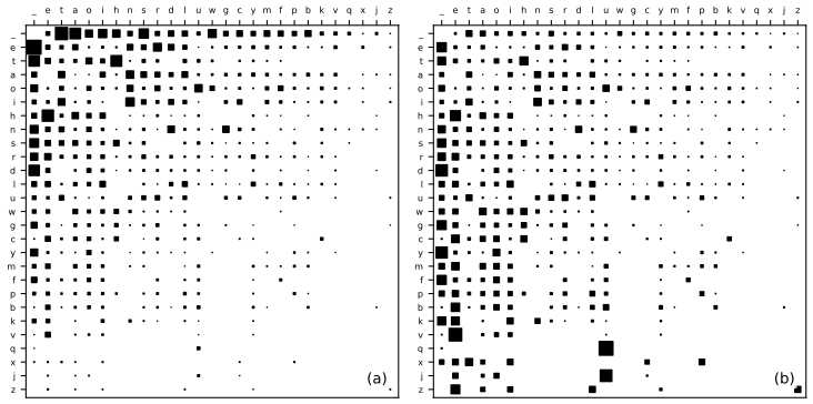
Figures and demonstrations. Every computed figure is reproduced by the Python code. Figures 2.9, 2.11, 2.15, 2.18 and 2.23 are cartoons, hand-drawn diagrams or figures from other papers and are not reproduced (2.9 is replaced by a computed version, Figure 2.S1). The book's texts (The Time Machine, the King James Bible) are replaced by a public-domain novel (Carroll's Alice's Adventures in Wonderland) in Figures 2.5, 2.16 and 2.17: same shapes, different numbers; the Harvard web graph of Supplementary Figure 2.3 is replaced by a simulated web graph. All other data are simulated. The book has no exercises for this chapter; Section 2.8 has three short practice problems with solutions.
Main reference
K. P. Murphy, Probabilistic Machine Learning: Advanced Topics, MIT Press (2023; December 2025 draft), Chapter 2, pages 5–62, and Supplementary Chapter 2 (book page: probml.github.io/pml-book/book2.html). Section, equation, figure numbers refer to this book. The explanations, derivations, figures and code are my own.
Companion courses
Much of this chapter restates Murphy's first volume in the same notation; where a result is proved in full there, these notes state it and link the proof.
- Probabilistic Machine Learning: An Introduction: Chapter 2, Chapter 3 (MVN, Bayes' rule for Gaussians, exponential family), Section 4.6.3 (Dirichlet-multinomial), Section 6.2 (KL divergence).
- Bayesian and Probabilistic Machine Learning (Bishop): Chapter 2, Section 13.1 (Markov models).
- All of Statistics: Chapter 1, Section 2.11, DKW inequality, Section 23.2.3 (convergence of Markov chains).
New here: information-form calculus and canonical potentials, the unknown-precision sensor fusion, exponential-family duality, PIT and KS, Markov chain convergence and PageRank, and all of Section 2.7.
The chapter at a glance
- 2.1 Axioms and Bayes' rule (gap 2.1).
- 2.2 Negative binomial (2.2), Student (2.3), chi-squared and inverse gamma (2.4), Pareto and Zipf (2.5), Dirichlet (2.6), Wishart (2.7), vMF and matrix normal (2.8).
- 2.3 Gaussian shells (2.9), marginals and conditionals (2.10), linear Gaussian systems (2.11), canonical potentials (2.12), missing data (2.13), unknown-precision sensor fusion (2.14).
- 2.4 Non-examples (2.15), cumulants (2.16), duality (2.17), MLE (2.18), maximum entropy (2.19).
- 2.5 Change of variables (2.20), PIT and KS (2.21).
- 2.6 Chapman–Kolmogorov, MLE, smoothing (2.22), stationary distributions (2.23), detailed balance and recurrence (2.24), PageRank (2.25).
- 2.7 f-divergences (2.26), TV and IPMs (2.27), MMD (2.28), density-ratio estimation (2.29).
Notation. \(\Ga\) is shape and rate; \(\bm\Lambda=\bm\Sigma^{-1}\) the precision, \(\bm\eta=\bm\Lambda\bm\mu\) the precision-weighted mean; for an exponential family \(\bm T(\bm x)\) is the sufficient statistic and \(A(\bm\eta)\) the log partition function. Markov chains use row vectors: \(\bm\pi_{t+1}=\bm\pi_t\bm A\).
Prerequisites. Chapters 2 to 4 of the first volume and block-matrix algebra.
2.1 Introduction
2.1.1 Probability space
p. 5 A probability space is a triple \((\Omega,\mathcal F,P)\): outcomes \(\Omega\), events \(\mathcal F\) and a measure \(P:\mathcal F\to[0,1]\) obeying the axioms of Section 2.1.4. For countable \(\Omega\) one takes all subsets as events; for uncountable \(\Omega\) one cannot define a countably additive \(P\) on all subsets that gives intervals their length, so a smaller \(\sigma\)-field is used.
See also: first volume, Section 2.1; All of Statistics, Chapter 1.
2.1.2 Discrete random variables
pp. 5–6 A random variable is a function \(X:\Omega\to\R\); its pmf is the pushforward \(p_X(a)=P[X=a]=P[X^{-1}(a)]\) (2.1). Two fair coin flips with \(X\) the number of heads give \(p_X=(\frac14,\frac12,\frac14)\): the outcomes \((T,H),(H,T)\) both map to 1.
2.1.3 Continuous random variables
pp. 6–7 For \(\Omega\subseteq\R\) the events form the Borel \(\sigma\)-field, generated by the half-lines \((-\infty,b]\); it contains every interval and point (2.2), see gap 2.1. A density \(p\ge0\) gives \(P([a,b])=\int_a^bp\) (2.3), and the cdf \(P_X(x)=\int_{-\infty}^xp_X\) (2.4) gives \(P(a\le X\le b)=P_X(b)-P_X(a)\) (2.5). A density is not a probability: it can exceed 1 (Figure 2.3a).
2.1.4 Probability axioms
p. 7 The Kolmogorov axioms: \(P[E]\ge0\), \(P[\Omega]=1\), and countable additivity \(P[\cup_iE_i]=\sum_iP[E_i]\) for disjoint events (2.6)–(2.7). They imply the complement rule \(P[E^c]=1-P[E]\) (2.8) and the addition rule \(P[E_1\cup E_2]=P[E_1]+P[E_2]-P[E_1\cap E_2]\) (2.9).
Filling the gap 2.1: the Borel \(\sigma\)-field contains all intervals; elementary consequences of the axioms pp. 6–8, (2.2), (2.8), (2.9)
Derivation
(2.2). The Borel \(\sigma\)-field contains \((-\infty,b]\) and is closed under complements and countable unions/intersections. Then \((a,b]=(-\infty,b]\cap(-\infty,a]^c\); \((b,\infty)=(-\infty,b]^c\); \(\{b\}=\bigcap_n(b-\frac1n,b]\); \((a,b)=\bigcup_n(a,b-\frac1n]\); \([a,b]=\{a\}\cup(a,b]\); \([a,b)=\{a\}\cup(a,b)\).
Consequences. (i) \(P[\emptyset]=0\): \(\Omega,\emptyset,\emptyset,\dots\) are disjoint with union \(\Omega\), so \(1=1+\sum_{i\ge2}P[\emptyset]\), and non-negativity forces \(P[\emptyset]=0\). (ii) Finite additivity (2.7) follows by padding with empty sets. (iii) \(E\) and \(E^c\) are disjoint with union \(\Omega\), so (2.8); and \(P[E]=1-P[E^c]\le1\) directly. (iv) Monotonicity: \(E\subseteq F\Rightarrow P[F]=P[E]+P[F\setminus E]\ge P[E]\). (v) Addition rule: \(E_1\cup E_2=E_1\sqcup(E_2\setminus E_1)\) and \(E_2=(E_1\cap E_2)\sqcup(E_2\setminus E_1)\), so \(P[E_1\cup E_2]=P[E_1]+P[E_2]-P[E_1\cap E_2]\). (vi) Total probability (2.14): for a partition \(A_i\), \(B=\sqcup_i(B\cap A_i)\) and \(P[B\cap A_i]=P[B\given A_i]P[A_i]\). Bayes' rule (2.15) is (2.11) read both ways, and (2.16) substitutes (2.14) for the denominator. \(\square\)
2.1.5–2.1.6 Conditional probability and Bayes' rule
pp. 7–8 \(P[E_1\given E_2]=P[E_1\cap E_2]/P[E_2]\) (2.10), independence \(P[E_1\cap E_2]=P[E_1]P[E_2]\) (2.12), conditional independence (2.13), and \[ p(X=k\given E)=\frac{p(E\given X=k)\,p(X=k)}{\sum_{k'}p(E\given X=k')\,p(X=k')}, \tag{2.16} \] posterior \(\propto\) likelihood \(\times\) prior, the denominator being the marginal likelihood; (2.17) is the continuous version. Worked examples: first volume, Section 2.3.
2.2 Some common probability distributions
p. 8 A catalogue. Most members are proved in the first volume, Chapter 2 and Bishop, Chapter 2; the notes add the proofs the book omits for the new ones.
2.2.1 Discrete distributions
pp. 9–10 Binomial (2.18), Bernoulli (2.19), categorical (2.20)–(2.21), multinomial (2.22)–(2.23), Poisson \(e^{-\lambda}\lambda^x/x!\) with mean and variance \(\lambda\) (2.24).
2.2.1.4 Negative binomial distribution
p. 10 Count successes (probability \(p\)) before the \(r\)-th failure: \[ \operatorname{NegBinom}(x\given r,p)=\binom{x+r-1}{x}(1-p)^rp^x,\qquad\E[x]=\frac{pr}{1-p},\quad\var[x]=\frac{pr}{(1-p)^2}. \tag{2.25, 2.26} \] Its variance exceeds its mean, \(\var=\E+\E^2/r\) (overdispersion); \(r=1\) is the geometric distribution. The book says \(\operatorname{Poi}(\lambda)=\lim_{r\to\infty}\operatorname{NegBinom}(r,\frac\lambda{1+\lambda})\): this has a slip, corrected below.
Filling the gap 2.2: the pmf, moments, the Poisson limit (with the right \(p\)) and the gamma-Poisson mixture p. 10, (2.25), (2.26)
Derivation
pmf. \(\{X=x\}\) means the \(r\)-th failure occurs at trial \(x+r\): that trial is a failure (\(1-p\)) and the first \(x+r-1\) trials hold \(x\) successes in \(\binom{x+r-1}x\) orders, each of probability \(p^x(1-p)^{r-1}\). For real \(r\) replace the coefficient by \(\Gamma(x+r)/(x!\Gamma(r))\).
Moments. The binomial series \((1-u)^{-r}=\sum_x\binom{x+r-1}xu^x\) gives \(G(s)=\E s^X=\big(\frac{1-p}{1-ps}\big)^r\). Then \(G'(1)=\frac{rp}{1-p}\), \(G''(1)=\frac{r(r+1)p^2}{(1-p)^2}\), and \(\var=G''(1)+G'(1)-G'(1)^2=\frac{rp}{(1-p)^2}\). With \(m=\E X\), \(p/(1-p)=m/r\), so \(\var=m+m^2/r\).
Poisson limit. With \(p=\lambda/(r+\lambda)\) the mean is \(\lambda\) for every \(r\), and \(G(s)=\big(1+\frac{\lambda(1-s)}r\big)^{-r}\to e^{-\lambda(1-s)}\), the Poisson generating function. With the book's \(p=\lambda/(1+\lambda)\) the mean is \(r\lambda\to\infty\): no limit. Correct statement: \(\operatorname{Poi}(\lambda)=\lim_{r\to\infty}\operatorname{NegBinom}(r,\frac{\lambda}{r+\lambda})\) (numerically, \(r=2000\), \(\lambda=2\): pmfs within \(10^{-3}\)).
Gamma-Poisson mixture (Practice problem 2.1): if \(\lambda\sim\Ga(r,\text{scale }\frac p{1-p})\) and \(X\given\lambda\sim\Poi(\lambda)\), \(p(x)=\int\frac{e^{-\lambda}\lambda^x}{x!}\frac{\lambda^{r-1}e^{-\lambda(1-p)/p}}{\Gamma(r)(p/(1-p))^r}\d\lambda=\frac{\Gamma(x+r)}{x!\Gamma(r)}(1-p)^rp^x\). "Contagious" counts are Poisson with a random rate, and \(\E^2/r\) is the variance of the rate. \(\square\)
2.2.2 Continuous distributions on \(\R\)
pp. 10–13 Gaussian (2.27)–(2.28), half-normal (2.29), Student with \(\nu\) degrees of freedom (2.30)–(2.31), Cauchy (\(\nu=1\), 2.34–2.35), Laplace (2.36). Student and Laplace have heavier tails than the Gaussian and are robust to outliers (Figure 2.1).
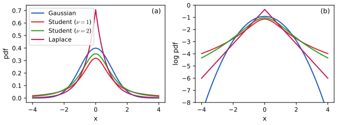
Filling the gap 2.3: the Student distribution as a Gaussian scale mixture: normaliser, moments, tails, Gaussian limit, multivariate case pp. 11–12, 17–18, (2.30), (2.31), (2.49)–(2.51)
Derivation
Scale mixture. Let \(\lambda\sim\Ga(\frac\nu2,\frac\nu2)\), \(x\given\lambda\sim\N(\mu,\sigma^2/\lambda)\), \(z=(x-\mu)/\sigma\). The joint is \(\propto\lambda^{1/2}e^{-\lambda z^2/2}\lambda^{\nu/2-1}e^{-\nu\lambda/2}\), and \(\int\lambda^{a-1}e^{-\lambda c}\d\lambda=\Gamma(a)c^{-a}\) gives \[ p(x)=\frac{(\nu/2)^{\nu/2}\Gamma(\frac{\nu+1}2)}{\Gamma(\frac\nu2)\sqrt{2\pi\sigma^2}}\Big(\frac2{\nu+z^2}\Big)^{\frac{\nu+1}2}=\frac{\Gamma(\frac{\nu+1}2)}{\Gamma(\frac\nu2)\sqrt{\nu\pi\sigma^2}}\Big(1+\frac{z^2}\nu\Big)^{-\frac{\nu+1}2}, \] which is (2.30) with \(Z=\sqrt{\nu\pi\sigma^2}\Gamma(\frac\nu2)/\Gamma(\frac{\nu+1}2)=\sqrt\nu\sigma B(\frac12,\frac\nu2)\) (2.31). The Student is a Gaussian with a random precision: an outlier is explained by a small \(\lambda\).
Moments, tails. The density decays like \(|x|^{-(\nu+1)}\), so \(\E|X|^k<\infty\) iff \(k<\nu\): mean for \(\nu>1\), variance for \(\nu>2\). By conditioning, \(\E X=\mu\) and \(\var X=\sigma^2\E[1/\lambda]=\frac\nu{\nu-2}\sigma^2\) (\(\E[1/\lambda]=b/(a-1)\), gap 2.4). Gaussian limit: \((1+z^2/\nu)^{-(\nu+1)/2}\to e^{-z^2/2}\) as \(\nu\to\infty\) and the mixing gamma (mean 1, variance \(2/\nu\)) concentrates at 1. Log-concavity: \((\log p)''=-\frac{\nu+1}{\nu\sigma^2}\frac{1-z^2/\nu}{(1+z^2/\nu)^2}>0\) for \(|z|>\sqrt\nu\), so the Student is never log-concave (it is unimodal).
Multivariate. With \(\bm x\given\lambda\sim\N(\bm\mu,\bm\Sigma/\lambda)\) and \(d=(\bm x-\bm\mu)^\T\bm\Sigma^{-1}(\bm x-\bm\mu)\) the same integral gives \(p(\bm x)=\frac{\Gamma(\frac{\nu+D}2)}{\Gamma(\frac\nu2)(\nu\pi)^{D/2}|\bm\Sigma|^{1/2}}(1+\frac d\nu)^{-\frac{\nu+D}2}\). So in (2.50) the normaliser has \(|\bm\Sigma|^{+1/2}\): the book prints \(|\bm\Sigma|^{-1/2}\) (numerical integration for \(D=2\), \(\nu=4\), \(|\bm\Sigma|=1.75\) gives \(Z=8.31\), matching \(+1/2\); \(-1/2\) gives 4.75). Covariance \(\E[1/\lambda]\bm\Sigma=\frac\nu{\nu-2}\bm\Sigma\) (2.51). \(\square\)
See also: first volume, Section 2.7.1; Bishop, Section 2.3.7.
2.2.2.6 Sub-Gaussian and super-Gaussian distributions
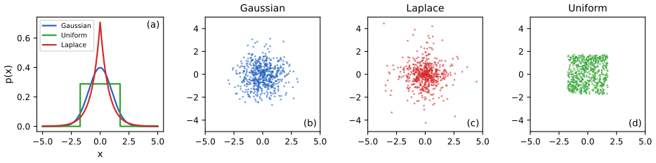
p. 13 The kurtosis \(\mu_4/\sigma^4\) (2.37) is 3 for a Gaussian. Positive excess kurtosis (Laplace: 3) is super-Gaussian (peaked, heavy tails); negative (uniform: \(-6/5\)) is sub-Gaussian (gap 2.4).
2.2.3 Continuous distributions on \(\R_+\)
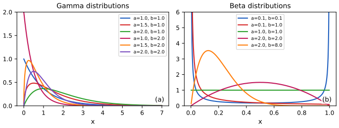
pp. 13–17 Gamma \(\Ga(x\given a,b)=\frac{b^a}{\Gamma(a)}x^{a-1}e^{-bx}\) (2.38)–(2.39); exponential \(\Ga(1,\lambda)\) (2.40); chi-squared \(\Ga(\frac\nu2,\frac12)\) (2.41), the law of a sum of \(\nu\) squared standard normals, so \(\E X^2=\sigma^2\), \(\var X^2=2\sigma^4\) for \(X\sim\N(0,\sigma^2)\) (2.42); inverse gamma, the law of \(1/X\) for \(X\sim\Ga(a,b)\) (2.43), with mean for \(a>1\), variance for \(a>2\); scaled inverse chi-squared \(\IG(\frac\nu2,\frac{\nu\sigma^2}2)\) (2.44)–(2.45).
Filling the gap 2.4: kurtosis values; the chi-squared law; inverse gamma moments pp. 13–15, (2.37), (2.41)–(2.45)
Derivation
Kurtosis. Gaussian: \(\E Z^4=3\sigma^4\), kurtosis 3. Laplace\((0,b)\): \(\E|X|^k=k!b^k\), so \(\mu_2=2b^2\), \(\mu_4=24b^4\), kurtosis 6 (excess 3). Uniform\((-a,a)\): \(\mu_2=a^2/3\), \(\mu_4=a^4/5\), kurtosis \(9/5\) (excess \(-6/5\)). Student, \(\nu>4\): \(\E[(X-\mu)^4]=3\sigma^4\E\lambda^{-2}=3\sigma^4\frac{\nu^2}{(\nu-2)(\nu-4)}\) (using \(\E\lambda^{-2}=\frac{b^2}{(a-1)(a-2)}\)), divided by \((\sigma^2\nu/(\nu-2))^2\): kurtosis \(3\frac{\nu-2}{\nu-4}\), excess \(\frac6{\nu-4}\).
Chi-squared. For \(Z\sim\N(0,1)\), \(Y=Z^2\) has density \(\phi(\sqrt y)/\sqrt y=(2\pi)^{-1/2}y^{-1/2}e^{-y/2}=\Ga(y\given\frac12,\frac12)\) (\(\Gamma(\frac12)=\sqrt\pi\)). The mgf of \(\Ga(a,b)\) is \((1-t/b)^{-a}\), so independent gammas with equal rate add shapes: \(\sum_{i\le\nu}Z_i^2\sim\Ga(\frac\nu2,\frac12)\) (2.41). \(\E Z^2=1\), \(\var Z^2=\E Z^4-1=2\), giving (2.42); \(\chi^2_\nu\) has mean \(\nu\), variance \(2\nu\).
Inverse gamma. If \(Y=1/X\), \(p_Y(y)=p_X(1/y)/y^2=\frac{b^a}{\Gamma(a)}y^{-(a+1)}e^{-b/y}\) (2.43). \(\E Y^k=b^k\Gamma(a-k)/\Gamma(a)\), finite iff \(a>k\): \(\E Y=\frac b{a-1}\), \(\var Y=\frac{b^2}{(a-1)^2(a-2)}\). (2.44)–(2.45) is (2.43) with \(a=\nu/2\), \(b=\nu\sigma^2/2\). \(\square\)
2.2.3.5 Pareto distribution
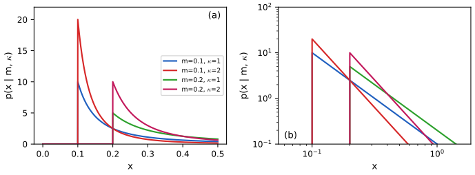
pp. 15–17 \(\operatorname{Pareto}(x\given m,\kappa)=\kappa m^\kappa x^{-(\kappa+1)}\ind(x\ge m)\) (2.46): a straight line of slope \(-(\kappa+1)\) on log-log axes (Figure 2.4b). It models heavy-tailed quantities (wealth, word counts); Zipf's law (2.47) says the word of rank \(r\) has frequency \(\propto r^{-a}\), \(a\approx1\) (Figure 2.5).
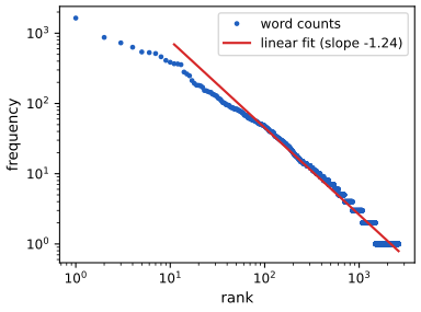
Filling the gap 2.5: moments and the 80-20 rule of the Pareto, and Zipf's law as a Pareto tail pp. 15–17, (2.46), (2.47)
Derivation
\(P(X>x)=(m/x)^\kappa\), so \(\E X^k=\kappa m^k/(\kappa-k)\) for \(k<\kappa\), infinite otherwise: the mean needs \(\kappa>1\), the variance \(\kappa>2\).
80-20. The richest fraction \(q\) lies above \(x_q=mq^{-1/\kappa}\); their share of the total is \(\frac{\int_{x_q}^\infty x\kappa m^\kappa x^{-\kappa-1}\d x}{\kappa m/(\kappa-1)}=(x_q/m)^{1-\kappa}=q^{1-1/\kappa}\). Setting \(q=0.2\), share \(0.8\): \(1-\frac1\kappa=\frac{\ln0.8}{\ln0.2}=0.1386\), \(\kappa=1.161\), the book's \(1.16\).
Zipf as Pareto. If rank \(r\) has frequency \(f=Cr^{-a}\), the number of words with frequency \(\ge f\) is \(r=(C/f)^{1/a}\): the distribution of word frequencies is Pareto with \(\kappa=1/a\). Zipf's \(a=1\) is the borderline \(\kappa=1\) (infinite mean); Figure 2.5's \(a=1.24\) gives \(\kappa\approx0.81\). \(\square\)
2.2.4 Continuous distributions on \([0,1]\)
p. 17 \(\operatorname{Beta}(x\given a,b)=x^{a-1}(1-x)^{b-1}/B(a,b)\) (2.48), the \(K=2\) Dirichlet (gap 2.6).
2.2.5 Multivariate continuous distributions
pp. 17–21 The multivariate Student is in gap 2.3; the von Mises–Fisher density \(\propto\exp(\kappa\bm\mu^\T\bm x)\) on the sphere (2.52)–(2.55) and the matrix normal (2.56)–(2.58) in gap 2.8; the Wishart (2.59)–(2.62) and inverse Wishart (2.63)–(2.66) in gap 2.7.
2.2.5.7 Dirichlet distribution
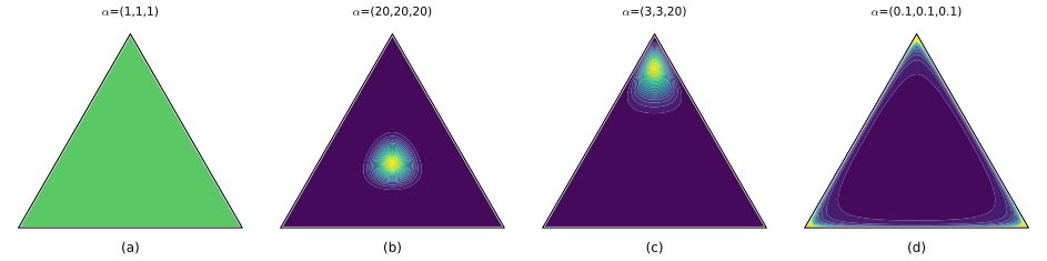
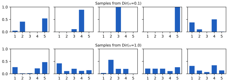
pp. 20–22 On the simplex \(\mathcal S_K\), \[ \Dir(\bm x\given\bm\alpha)=\frac1{B(\bm\alpha)}\prod_kx_k^{\alpha_k-1},\qquad B(\bm\alpha)=\frac{\prod_k\Gamma(\alpha_k)}{\Gamma(\alpha_0)},\ \alpha_0=\sum_k\alpha_k, \tag{2.68, 2.69} \] with moments (2.70). For \(\alpha_k=\alpha/K\): \(\E x_k=1/K\), \(\var x_k=\frac{K-1}{K^2(\alpha+1)}\). \(\Dir(20,20,20)\) and \(\Dir(1,1,1)\) share the mean \((\frac13,\frac13,\frac13)\) but the first is sure the die is fair (aleatoric uncertainty only) and the second admits any bias (epistemic uncertainty).
Filling the gap 2.6: the Dirichlet normaliser, moments and mode via the gamma construction pp. 17, 20, (2.48)–(2.50), (2.68)–(2.70)
Derivation
Construction. Let \(G_k\sim\Ga(\alpha_k,1)\) be independent. Set \(S=\sum G_k\), \(X_k=G_k/S\) (\(k<K\)); the inverse map \(g_k=sx_k\) has Jacobian \(s^{K-1}\). The joint density of \((S,X_1,\dots,X_{K-1})\) is \[ \frac{s^{\alpha_0-K}e^{-s}s^{K-1}}{\prod_k\Gamma(\alpha_k)}\prod_kx_k^{\alpha_k-1}=\Big[\frac{s^{\alpha_0-1}e^{-s}}{\Gamma(\alpha_0)}\Big]\Big[\frac{\Gamma(\alpha_0)}{\prod\Gamma(\alpha_k)}\prod_kx_k^{\alpha_k-1}\Big]. \] So \(S\sim\Ga(\alpha_0,1)\) is independent of \(\bm X\), and \(\bm X\) has density \(\prod x_k^{\alpha_k-1}/B(\bm\alpha)\): this proves (2.69) and \(\bm X\sim\Dir(\bm\alpha)\).
Moments. \(G_k=SX_k\) with \(S\perp\bm X\): \(\alpha_k=\alpha_0\E X_k\), and \(\alpha_k(\alpha_k+1)=\alpha_0(\alpha_0+1)\E X_k^2\), so \(\var X_k=\frac{\alpha_k(\alpha_k+1)}{\alpha_0(\alpha_0+1)}-\frac{\alpha_k^2}{\alpha_0^2}=\frac{\alpha_k(\alpha_0-\alpha_k)}{\alpha_0^2(\alpha_0+1)}\); likewise \(\operatorname{cov}(X_j,X_k)=-\frac{\alpha_j\alpha_k}{\alpha_0^2(\alpha_0+1)}\). For \(\alpha_k=\alpha/K\): \(\frac{K-1}{K^2(\alpha+1)}\).
Mode. Maximising \(\sum(\alpha_k-1)\log x_k\) on the simplex: \((\alpha_k-1)/x_k=\lambda\), so \(x_k=\frac{\alpha_k-1}{\alpha_0-K}\) when all \(\alpha_k>1\); if some \(\alpha_k<1\) the density is unbounded at that face (Figure 2.6d). \(\square\)
2.2.5.5–2.2.5.6 Wishart and inverse Wishart
pp. 19–20 The Wishart is the multivariate gamma, \(\Wi(\bm\Sigma\given\bm S,\nu)=\frac1Z|\bm\Sigma|^{(\nu-D-1)/2}\exp(-\frac12\Tr(\bm S^{-1}\bm\Sigma))\), mean \(\nu\bm S\), mode \((\nu-D-1)\bm S\) (2.59)–(2.61); the scatter matrix of \(N\) \(\N(\bm0,\bm\Sigma)\) vectors is \(\Wi(\bm\Sigma,N)\). The inverse Wishart is the law of \(\bm\Sigma\) when \(\bm\Sigma^{-1}\sim\Wi(\bm S^{-1},\nu)\), mean \(\bm S/(\nu-D-1)\), mode \(\bm S/(\nu+D+1)\) (2.63)–(2.65). The book's normalisers (2.60), (2.64) have the wrong sign of the exponent of \(|\bm S|\).
Filling the gap 2.7: Wishart and inverse Wishart: normalisers, moments, modes, the scatter-matrix theorem, one dimension pp. 19–20, (2.59)–(2.66)
Derivation
Multivariate gamma integral. For \(\bm A\succ0\), \(a>\frac{D-1}2\): \(\int_{\bm S\succ0}|\bm S|^{a-\frac{D+1}2}e^{-\Tr(\bm A\bm S)}\d\bm S=\Gamma_D(a)|\bm A|^{-a}\), \(\Gamma_D(a)=\pi^{D(D-1)/4}\prod_{j=1}^D\Gamma(a-\frac{j-1}2)\) (*). (Reduce to \(\bm A=\bm I\) by \(\bm S\mapsto\bm A^{-1/2}\bm S\bm A^{-1/2}\), Jacobian \(|\bm A|^{-(D+1)/2}\), then Cholesky \(\bm S=\bm L\bm L^\T\), Jacobian \(2^D\prod l_{ii}^{D-i+1}\); Muirhead 1982, Thm 2.1.11.)
Normaliser. (*) with \(a=\nu/2\), \(\bm A=\frac12\bm S^{-1}\): \(Z=\Gamma_D(\frac\nu2)|\frac12\bm S^{-1}|^{-\nu/2}=|\bm S|^{+\nu/2}2^{\nu D/2}\Gamma_D(\frac\nu2)\). The book's (2.60) has \(|\bm S|^{-\nu/2}\).
Laplace transform and mean. (*) with \(\bm A=\frac12\bm S^{-1}+\bm T\): \(\E e^{-\Tr(\bm T\bm\Sigma)}=|\bm I+2\bm S\bm T|^{-\nu/2}\). Differentiating at \(\bm T=\bm0\): \(\E\bm\Sigma=\nu\bm S\).
Scatter-matrix theorem. For \(\bm x_n\sim\N(\bm0,\bm\Sigma_0)\) independent, \(\E e^{-\Tr(\bm T\sum\bm x_n\bm x_n^\T)}=\prod_n\E e^{-\bm x_n^\T\bm T\bm x_n}=|\bm I+2\bm\Sigma_0\bm T|^{-N/2}\) (a Gaussian integral): the Laplace transform of \(\Wi(\bm\Sigma_0,N)\). Laplace transforms determine laws on the cone, so the scatter matrix is Wishart for \(N\ge D\); its \((1,1)\) entry is \(\Sigma_{0,11}\chi^2_N\).
Mode. The log density's gradient \(\frac{\nu-D-1}2\bm\Sigma^{-1}-\frac12\bm S^{-1}\) vanishes at \((\nu-D-1)\bm S\) (a maximum iff \(\nu>D+1\)).
One dimension. \(D=1\), scale \(s\): density \(\propto\lambda^{(\nu-2)/2}e^{-\lambda/(2s)}\), i.e. \(\Ga(\frac\nu2,\text{rate }\frac1{2s})\); \(s=1\) is \(\chi^2_\nu\). The book's (2.62) writes \(\Wi(\lambda\given s^{-1},\nu)=\Ga(\frac\nu2,\frac1{2s})\) and says \(s=2\) gives \(\chi^2\): with the convention of (2.59) the argument should be \(s\), and the chi-squared case is \(s=1\).
Inverse Wishart. \(\bm W\mapsto\bm W^{-1}\) has Jacobian \(|\bm W|^{-(D+1)}\), so if \(\bm W\sim\Wi(\bm\Psi^{-1},\nu)\), \(\bm\Sigma=\bm W^{-1}\) has density \(\propto|\bm\Sigma|^{-(\nu+D+1)/2}e^{-\frac12\Tr(\bm\Psi\bm\Sigma^{-1})}\) with \(Z_{IW}=|\bm\Psi|^{-\nu/2}2^{\nu D/2}\Gamma_D(\frac\nu2)\) (the book's (2.64) has \(+\nu/2\)). Mode: \(-\frac{\nu+D+1}2\bm\Sigma^{-1}+\frac12\bm\Sigma^{-1}\bm\Psi\bm\Sigma^{-1}=0\) at \(\bm\Psi/(\nu+D+1)\). Mean (integer \(\nu=N\)): \(\bm W=\bm X^\T\bm X\), \(1/(\bm W^{-1})_{11}=\bm x_1^\T(\bm I-\bm P)\bm x_1\sim\chi^2_{N-D+1}\) by Cochran (\(\bm P\) projects on the other \(D-1\) columns), and \(\E[1/\chi^2_k]=\frac1{k-2}\), so \(\E(\bm W^{-1})_{11}=\frac1{N-D-1}\); orthogonal invariance of \(\Wi(\bm I,N)\) makes \(\E\bm W^{-1}\) a multiple of \(\bm I\); \(\bm\Sigma=\bm\Psi^{1/2}\bm W^{-1}\bm\Psi^{1/2}\) gives \(\bm\Psi/(\nu-D-1)\) (2.65) (real \(\nu\): Bartlett decomposition, Muirhead Sec. 3.2). \(D=1\): \(\propto\sigma^{-(\nu+2)/2}e^{-s/(2\sigma)}=\IG(\frac\nu2,\frac s2)\) (2.66). All of this was confirmed numerically (normalisers, scatter-matrix law, modes, inverse mean). \(\square\)
Filling the gap 2.8: the von Mises–Fisher normaliser and the matrix normal pp. 18–19, (2.52)–(2.58)
Derivation
vMF. Take \(\bm\mu\) as the pole, \(\bm x=(\cos\theta,\sin\theta\,\bm u)\); the surface measure is \(\sin^{D-2}\theta\d\theta\d\sigma_{D-2}(\bm u)\), so \(Z=|S^{D-2}|\int_0^\pi e^{\kappa\cos\theta}\sin^{D-2}\theta\d\theta\), \(|S^{D-2}|=2\pi^{(D-1)/2}/\Gamma(\frac{D-1}2)\). The Poisson integral \(I_\nu(\kappa)=\frac{(\kappa/2)^\nu}{\sqrt\pi\Gamma(\nu+\frac12)}\int_0^\pi e^{\kappa\cos\theta}\sin^{2\nu}\theta\d\theta\) with \(\nu=\frac D2-1\) gives \(Z=(2\pi)^{D/2}\kappa^{1-D/2}I_{D/2-1}(\kappa)\) (2.53); \(D=2\): \(2\pi I_0(\kappa)\) (2.55).
Matrix normal. \(\Tr(\bm A^\T\bm B\bm A\bm C)=\operatorname{vec}(\bm A)^\T(\bm C\otimes\bm B)\operatorname{vec}(\bm A)\) turns the exponent of (2.56) into \(-\frac12\operatorname{vec}(\bm X-\bm M)^\T(\bm V\otimes\bm U^{-1})\operatorname{vec}(\bm X-\bm M)\): a Gaussian with precision \(\bm V\otimes\bm U^{-1}=(\bm V^{-1}\otimes\bm U)^{-1}\), i.e. (2.57). With \(|\bm V^{-1}\otimes\bm U|=|\bm V|^{-n}|\bm U|^p\) the normaliser is \(|\bm V|^{n/2}/((2\pi)^{np/2}|\bm U|^{p/2})\). Using \(\tilde{\bm V}=\bm V^{-1}\) (2.58) is the same density. (Checked for \(n=3,p=2\).) \(\square\)
2.3 Gaussian joint distributions
p. 22 The multivariate Gaussian is closed under marginals, conditionals, linear maps and products, is the maximum entropy law for given mean and covariance (gap 2.19), and is often a fair model.
See also: first volume, Section 3.2 and Section 3.3 (MVN, Bayes' rule for Gaussians, sensor fusion); Bishop, Section 2.3.
2.3.1 The multivariate normal
2.3.1.1 Definition
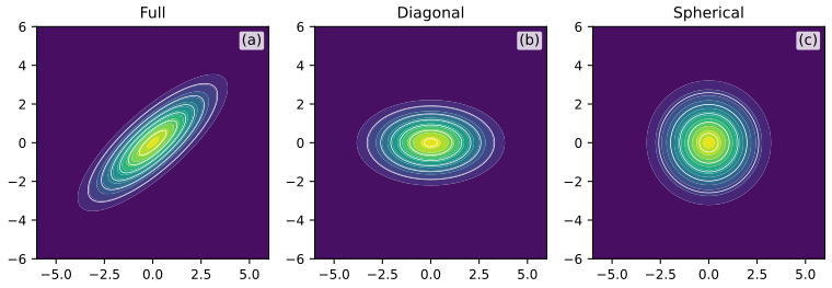
pp. 22–23 \(\N(\bm x\given\bm\mu,\bm\Sigma)=(2\pi)^{-D/2}|\bm\Sigma|^{-1/2}\exp(-\frac12(\bm x-\bm\mu)^\T\bm\Sigma^{-1}(\bm x-\bm\mu))\) (2.71), the exponent being the squared Mahalanobis distance (2.72); in 2-d (2.73). Full covariances have \(D(D+1)/2\) parameters and elliptical level sets, diagonal ones \(D\) and axis-aligned ellipses, spherical ones one and circles (Figure 2.8).
2.3.1.2 Gaussian shells
pp. 23–24 In high dimension a draw from \(\N(\bm0,\bm I_D)\) has norm concentrated near \(\sqrt D\), not near the mode. The book's argument has a small slip and states the shell thickness as \(O(\sigma D^{1/4})\); it is \(O(\sigma)\).
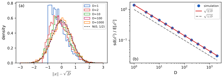
Filling the gap 2.9: the Gaussian soap bubble, quantitatively pp. 23–24, (2.74)
Derivation
\(d^2=\sum x_i^2\sim\chi^2_D\): \(\E d^2=D\) and, since \(\var x_i^2=\E x_i^4-1=2\), \(\var d^2=2D\) (the book gets \(D\) from \(\var x_i^2=1\)). So \(\operatorname{std}(d^2)/\E d^2=\sqrt{2/D}\to0\), the conclusion of (2.74). Non-asymptotically (Laurent–Massart 2000) \(P(|d^2-D|\ge2\sqrt{Dt}+2t)\le2e^{-t}\).
Thickness. \(d-\sqrt D=\frac{d^2-D}{d+\sqrt D}\), with numerator of size \(\sqrt{2D}\) and denominator \(\approx2\sqrt D\): the standard deviation of \(d\) tends to \(1/\sqrt2\), so the radial thickness is \(O(\sigma)\) (simulation at \(D=400\): 0.710; Figure 2.S1a). Relative to the radius it is \(O(D^{-1/2})\).
Atypical mode. \(\log p(\bm0)-\log p(\bm x)=d^2/2\approx D/2\): a typical sample has density \(e^{-D/2}\) times the peak. \(\square\)
2.3.1.3–2.3.1.6 Marginals, conditionals, information form
pp. 24–28 For \(\bm x=(\bm x_1,\bm x_2)\): \(p(\bm x_1)=\N(\bm\mu_1,\bm\Sigma_{11})\) (2.76)–(2.77) and \[ p(\bm x_1\given\bm x_2)=\N\big(\bm\mu_1+\bm\Sigma_{12}\bm\Sigma_{22}^{-1}(\bm x_2-\bm\mu_2),\ \bm\Sigma_{11}-\bm\Sigma_{12}\bm\Sigma_{22}^{-1}\bm\Sigma_{21}\big). \tag{2.78} \] In information form (\(\bm\Lambda=\bm\Sigma^{-1}\), \(\bm\eta=\bm\Lambda\bm\mu\), (2.80)–(2.83)): \[ p(\bm x_1\given\bm x_2)=\N_c(\bm\eta_1-\bm\Lambda_{12}\bm x_2,\bm\Lambda_{11}),\quad p(\bm x_1)=\N_c(\bm\eta_1-\bm\Lambda_{12}\bm\Lambda_{22}^{-1}\bm\eta_2,\ \bm\Lambda_{11}-\bm\Lambda_{12}\bm\Lambda_{22}^{-1}\bm\Lambda_{21}), \tag{2.84, 2.86} \] so marginalisation is easy in moment form and conditioning in information form.
Filling the gap 2.10: marginals, conditionals and information form via decorrelation and the block inverse pp. 24–28, (2.76)–(2.79), (2.84)–(2.93), (2.102)–(2.117)
Derivation
Block inverse. \(\bm M=\begin{pmatrix}\bm E&\bm F\\\bm G&\bm H\end{pmatrix}=\begin{pmatrix}\bm I&\bm F\bm H^{-1}\\\bm0&\bm I\end{pmatrix}\begin{pmatrix}\bm M/\bm H&\bm0\\\bm0&\bm H\end{pmatrix}\begin{pmatrix}\bm I&\bm0\\\bm H^{-1}\bm G&\bm I\end{pmatrix}\), \(\bm M/\bm H=\bm E-\bm F\bm H^{-1}\bm G\); inverting the factors gives (2.89), swapping roles (2.90), and equating the \((1,1)\) blocks the matrix inversion lemma (2.93).
Marginals. A linear image \(\bm A\bm x\) is \(\N(\bm A\bm\mu,\bm A\bm\Sigma\bm A^\T)\) (characteristic function); selecting coordinates gives (2.76)–(2.77) without integration. (The book points to Section 2.3.1.5 for this, which derives only the conditional.)
Conditional by decorrelation. Let \(\bm B=\bm\Sigma_{12}\bm\Sigma_{22}^{-1}\), \(\bm u=\bm x_1-\bm B\bm x_2\). \((\bm u,\bm x_2)\) is jointly Gaussian with \(\operatorname{cov}(\bm u,\bm x_2)=\bm\Sigma_{12}-\bm B\bm\Sigma_{22}=\bm0\), hence independent (block-diagonal covariance gives a factorising density); \(\operatorname{cov}(\bm u)=\bm\Sigma_{11}-\bm\Sigma_{12}\bm\Sigma_{22}^{-1}\bm\Sigma_{21}\). Since \(\bm x_1=\bm u+\bm B\bm x_2\), given \(\bm x_2\) only the second term is fixed: (2.78), and (2.79) by symmetry.
Information form. By (2.89) applied to \(\bm\Lambda\): \(\bm\Lambda_{11}=(\bm\Sigma/\bm\Sigma_{22})^{-1}\) (so the conditional precision is \(\bm\Lambda_{11}\), (2.107)) and \(\bm\Lambda_{12}=-\bm\Lambda_{11}\bm B\). The conditional precision-weighted mean is \(\bm\Lambda_{11}(\bm\mu_1+\bm B(\bm x_2-\bm\mu_2))=\bm\Lambda_{11}\bm\mu_1+\bm\Lambda_{12}\bm\mu_2-\bm\Lambda_{12}\bm x_2=\bm\eta_1-\bm\Lambda_{12}\bm x_2\) (2.109). For the marginal, (2.90) gives \(\Sigma_{11}=(\bm\Lambda/\bm\Lambda_{22})^{-1}\): the marginal precision is \(\bm\Lambda_{11}-\bm\Lambda_{12}\bm\Lambda_{22}^{-1}\bm\Lambda_{21}\) (2.116), and times \(\bm\mu_1\) it equals \(\bm\eta_1-\bm\Lambda_{12}\bm\Lambda_{22}^{-1}\bm\eta_2\) (substitute \(\bm\eta_2=\bm\Lambda_{21}\bm\mu_1+\bm\Lambda_{22}\bm\mu_2\)): (2.117). Duality: a Schur complement of \(\bm\Sigma\) is the conditional covariance; a Schur complement of \(\bm\Lambda\) is the marginal precision. All four formulas agree with brute-force evaluation for a random \(5\times5\) covariance. \(\square\)
2.3.2 Linear Gaussian systems
pp. 28–30 With \(p(\bm z)=\N(\breve{\bm\mu},\breve{\bm\Sigma})\), \(p(\bm y\given\bm z)=\N(\bm W\bm z+\bm b,\bm\Omega)\) (2.118–2.119) the joint is Gaussian with blocks \(\breve{\bm\Sigma}\), \(\bm C^\T=\breve{\bm\Sigma}\bm W^\T\), \(\bm S=\bm W\breve{\bm\Sigma}\bm W^\T+\bm\Omega\) (2.120), and Bayes' rule for Gaussians is \[ \hat{\bm\mu}=\breve{\bm\mu}+\bm K(\bm y-\bm m),\quad\hat{\bm\Sigma}=\breve{\bm\Sigma}-\bm K\bm C^\T=\breve{\bm\Sigma}-\bm K\bm S\bm K^\T,\quad\bm K=\bm C\bm S^{-1},\ \bm m=\bm W\breve{\bm\mu}+\bm b, \tag{2.121–2.126} \] equivalently \(\hat{\bm\Sigma}=(\breve{\bm\Sigma}^{-1}+\bm W^\T\bm\Omega^{-1}\bm W)^{-1}\), \(\hat{\bm\mu}=\hat{\bm\Sigma}[\bm W^\T\bm\Omega^{-1}(\bm y-\bm b)+\breve{\bm\Sigma}^{-1}\breve{\bm\mu}]\) (2.127–2.128), costing \(O(L^3)\) not \(O(D^3)\); and the evidence is \(p(\bm y)=\N(\bm m,\bm S)\) (2.129).
Filling the gap 2.11: joint, posterior in Kalman and information form, their equivalence, and the evidence pp. 28–29, (2.120)–(2.129)
Derivation
Joint. \(\bm y=\bm W\bm z+\bm b+\bm\varepsilon\), \(\bm\varepsilon\sim\N(\bm0,\bm\Omega)\perp\bm z\): \((\bm z,\bm y)\) is a linear image of \((\bm z,\bm\varepsilon)\), hence Gaussian, with \(\operatorname{cov}(\bm z,\bm y)=\breve{\bm\Sigma}\bm W^\T\), \(\operatorname{cov}\bm y=\bm S\).
Kalman form. (2.78) gives mean \(\breve{\bm\mu}+\bm C\bm S^{-1}(\bm y-\bm m)\), covariance \(\breve{\bm\Sigma}-\bm C\bm S^{-1}\bm C^\T\), and \(\bm K\bm S\bm K^\T=\bm C\bm S^{-1}\bm S\bm S^{-1}\bm C^\T=\bm K\bm C^\T\) (2.125).
Information form. The log posterior is \(-\frac12(\bm z-\breve{\bm\mu})^\T\breve{\bm\Sigma}^{-1}(\bm z-\breve{\bm\mu})-\frac12(\bm y-\bm W\bm z-\bm b)^\T\bm\Omega^{-1}(\cdot)+\mathrm{const}\): quadratic part \(\breve{\bm\Sigma}^{-1}+\bm W^\T\bm\Omega^{-1}\bm W\), linear part \(\breve{\bm\Sigma}^{-1}\breve{\bm\mu}+\bm W^\T\bm\Omega^{-1}(\bm y-\bm b)\): (2.127)–(2.128).
Equivalence. Woodbury (2.93) gives the covariances. Push-through: \((\breve{\bm\Sigma}^{-1}+\bm W^\T\bm\Omega^{-1}\bm W)\breve{\bm\Sigma}\bm W^\T=\bm W^\T\bm\Omega^{-1}(\bm\Omega+\bm W\breve{\bm\Sigma}\bm W^\T)\), so \(\bm K=\hat{\bm\Sigma}\bm W^\T\bm\Omega^{-1}\). With \(\hat{\bm\Sigma}\breve{\bm\Sigma}^{-1}=\bm I-\bm K\bm W\): \(\hat{\bm\Sigma}[\breve{\bm\Sigma}^{-1}\breve{\bm\mu}+\bm W^\T\bm\Omega^{-1}(\bm y-\bm b)]=(\bm I-\bm K\bm W)\breve{\bm\mu}+\bm K(\bm y-\bm b)=\breve{\bm\mu}+\bm K(\bm y-\bm m)\).
Evidence. \(p(\bm z\given\bm y)=p(\bm z)p(\bm y\given\bm z)/p(\bm y)\) holds for every \(\bm z\), so \(\log p(\bm y)=\log p(\bm z)+\log p(\bm y\given\bm z)-\log p(\bm z\given\bm y)\) for any \(\bm z\), equal to \(\log\N(\bm y\given\bm m,\bm S)\) (checked for \(L=3\), \(D=4\)). \(\square\)
2.3.2.3 Example: sensor fusion with known measurement noise
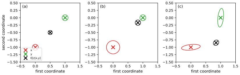
p. 30 Two measurements \(\bm x\sim\N(\bm z,\bm\Sigma_x)\), \(\bm y\sim\N(\bm z,\bm\Sigma_y)\) form a linear Gaussian system with \(\bm W=[\bm I;\bm I]\), \(\bm\Omega=\diag(\bm\Sigma_x,\bm\Sigma_y)\); with a broad prior \(\E[\bm z\given\bm x,\bm y]=(\bm\Sigma_x^{-1}+\bm\Sigma_y^{-1})^{-1}(\bm\Sigma_x^{-1}\bm x+\bm\Sigma_y^{-1}\bm y)\). Figure 2.10 (\(\bm x=(0,-1)\), \(\bm y=(1,0)\)): (a) equal noise \(0.01\bm I\): the midpoint \((0.5,-0.5)\); (b) \(\bm\Sigma_x=0.05\bm I\), \(\bm\Sigma_y=0.01\bm I\): precisions 20 and 100, mean \((0.833,-0.167)\); (c) \(\bm\Sigma_x=0.01\begin{pmatrix}10&1\\1&1\end{pmatrix}\), \(\bm\Sigma_y=0.01\begin{pmatrix}1&1\\1&10\end{pmatrix}\): \(\bm\Sigma_x^{-1}+\bm\Sigma_y^{-1}=\frac{100}9\begin{pmatrix}11&-2\\-2&11\end{pmatrix}\), \(\bm\Sigma_x^{-1}\bm x+\bm\Sigma_y^{-1}\bm y=\frac{100}9(11,-11)^\T\), so the mean is \((\frac{11}{13},-\frac{11}{13})\): vertically near \(x\)'s \(-1\), horizontally near \(y\)'s 1.
2.3.3 A general calculus for linear Gaussian systems
pp. 30–33 Inference in Gaussian graphical models uses potentials \(\phi(\bm x;g,\bm h,\bm K)=\exp(g+\bm h^\T\bm x-\frac12\bm x^\T\bm K\bm x)\) with \(\bm K=\bm\Sigma^{-1}\), \(\bm h=\bm K\bm\mu\), \(g=\log p-\frac12\bm\mu^\T\bm K\bm\mu\) (2.131)–(2.135). Operations: multiplication/division add/subtract \((g,\bm h,\bm K)\) (2.136–2.137); marginalising \(\bm x_1\): \(\hat{\bm K}=\bm K_{22}-\bm K_{21}\bm K_{11}^{-1}\bm K_{12}\), \(\hat{\bm h}=\bm h_2-\bm K_{21}\bm K_{11}^{-1}\bm h_1\), \(\hat g=g+\frac12(n_1\log2\pi-\log|\bm K_{11}|+\bm h_1^\T\bm K_{11}^{-1}\bm h_1)\) (2.139–2.142); conditioning on \(\bm y\) (2.143–2.144); converting a CPD \(\N(\bm x\given\bm\mu+\bm B^\T\bm u,\bm\Sigma)\) to a potential (2.145–2.153); and the product of two Gaussians (2.154)–(2.159).
Filling the gap 2.12: the potential calculus and the product of Gaussians, with the constant pp. 31–33, (2.131)–(2.159)
Derivation
Canonical form. \(-\frac12(\bm x-\bm\mu)^\T\bm K(\bm x-\bm\mu)=-\frac12\bm x^\T\bm K\bm x+\bm\mu^\T\bm K\bm x-\frac12\bm\mu^\T\bm K\bm\mu\). Products: exponents add (after zero-padding).
Marginalisation. \(\phi=e^{g+\bm h_2^\T\bm x_2-\frac12\bm x_2^\T\bm K_{22}\bm x_2}\,e^{\bm a^\T\bm x_1-\frac12\bm x_1^\T\bm K_{11}\bm x_1}\), \(\bm a=\bm h_1-\bm K_{12}\bm x_2\), and \(\int e^{\bm a^\T\bm x-\frac12\bm x^\T\bm K_{11}\bm x}\d\bm x=(2\pi)^{n_1/2}|\bm K_{11}|^{-1/2}e^{\frac12\bm a^\T\bm K_{11}^{-1}\bm a}\); expanding \(\frac12\bm a^\T\bm K_{11}^{-1}\bm a\) in \(\bm x_2\) gives \(\hat g,\hat{\bm h},\hat{\bm K}\) (needs \(\bm K_{11}\succ0\)).
Conditioning. Fixing \(\bm y\): \(\bm x^\T(\bm h_X-\bm K_{XY}\bm y)-\frac12\bm x^\T\bm K_{XX}\bm x\) plus the constant \(g+\bm h_Y^\T\bm y-\frac12\bm y^\T\bm K_{YY}\bm y\).
CPD. Expanding \(-\frac12(\bm x-\bm\mu-\bm B^\T\bm u)^\T\bm\Sigma^{-1}(\cdot)\): \(\bm K=\begin{pmatrix}\bm I\\-\bm B\end{pmatrix}\bm\Sigma^{-1}\begin{pmatrix}\bm I&-\bm B^\T\end{pmatrix}\) (2.150), \(\bm h=(\bm\Sigma^{-1}\bm\mu;-\bm B\bm\Sigma^{-1}\bm\mu)\) (2.149), \(g=-\frac12\bm\mu^\T\bm\Sigma^{-1}\bm\mu+\log c\). Scalar case: \(\bm K=\frac1{\sigma^2}\begin{pmatrix}1&-b\\-b&b^2\end{pmatrix}\); the book's (2.153) prints \(\frac1\sigma\), a slip.
Product. Adding \(\bm K\) and \(\bm h\): precision \(\bm\Sigma_1^{-1}+\bm\Sigma_2^{-1}\), precision-weighted mean \(\bm\Sigma_1^{-1}\bm\mu_1+\bm\Sigma_2^{-1}\bm\mu_2\) (2.155–2.156). Since \(\bm\Sigma_1^{-1}+\bm\Sigma_2^{-1}=\bm\Sigma_1^{-1}(\bm\Sigma_1+\bm\Sigma_2)\bm\Sigma_2^{-1}=\bm\Sigma_2^{-1}(\bm\Sigma_1+\bm\Sigma_2)\bm\Sigma_1^{-1}\), \(\bm\Sigma_3=\bm\Sigma_1(\bm\Sigma_1+\bm\Sigma_2)^{-1}\bm\Sigma_2\) (2.157), and \(\bm\Sigma_3\bm\Sigma_1^{-1}=\bm\Sigma_2(\bm\Sigma_1+\bm\Sigma_2)^{-1}\), \(\bm\Sigma_3\bm\Sigma_2^{-1}=\bm\Sigma_1(\bm\Sigma_1+\bm\Sigma_2)^{-1}\) give (2.158). The constant: \(\N(\bm x\given\bm\mu_1,\bm\Sigma_1)\N(\bm x\given\bm\mu_2,\bm\Sigma_2)=\N(\bm\mu_1\given\bm\mu_2,\bm\Sigma_1+\bm\Sigma_2)\N(\bm x\given\bm\mu_3,\bm\Sigma_3)\) (it integrates to the convolution density). All checked numerically on random matrices. \(\square\)
Supplement 2.1 More fun with MVNs (supplement)
Supplement 2.1.1 Inference in the presence of missing data
Supp. p. 15 If only \(\bm y_1\) of \(\bm y=(\bm y_1,\bm y_2)\) is observed, with \(\bm W=(\bm W_1;\bm W_2)\), \(\bm b=(\bm b_1;\bm b_2)\) and noise blocks \(\bm\Sigma_{ij}\), then \(\bm\Sigma_{z|1}^{-1}=\bm\Sigma_z^{-1}+\bm W_1^\T\bm\Sigma_{11}^{-1}\bm W_1\), \(\bm\mu_{z|1}=\bm\Sigma_{z|1}[\bm W_1^\T\bm\Sigma_{11}^{-1}(\bm y_1-\bm b_1)+\bm\Sigma_z^{-1}\bm\mu_z]\) (Supp. 2.4–2.5).
Filling the gap 2.13: posterior from partial observations Supp. p. 15, (2.3)–(2.5)
Derivation
\((\bm z,\bm y_1,\bm y_2)\) is Gaussian, so marginalising \(\bm y_2\) just reads off a sub-block (gap 2.10): \(\bm y_1\given\bm z\sim\N(\bm W_1\bm z+\bm b_1,\bm\Sigma_{11})\) whatever \(\bm W_2,\bm b_2,\bm\Sigma_{12},\bm\Sigma_{22}\) are. That is a linear Gaussian system, and (2.127)–(2.128) of gap 2.11 with \(\bm\Omega=\bm\Sigma_{11}\) give the result. \(\bm y_2\) is predicted afterwards from \(p(\bm y_2\given\bm y_1)\). (Checked against marginalise-then-condition on a random system.) \(\square\)
Supplement 2.1.2 Sensor fusion with unknown measurement noise
Supp. pp. 15–18 Now the precisions \(\lambda_x,\lambda_y\) are unknown. Scalar \(z\), flat prior, two readings each: \(x=(1.1,1.9)\), \(y=(2.9,4.1)\), so \(\bar x=1.5\), \(s_x^2=0.16\), \(\bar y=3.5\), \(s_y^2=0.36\) (divisor \(N\)).
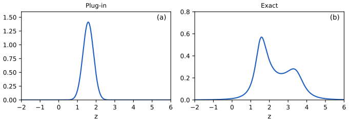
Plug-in. The joint MLE solves \(\hat z=\frac{N_x\hat\lambda_x\bar x+N_y\hat\lambda_y\bar y}{N_x\hat\lambda_x+N_y\hat\lambda_y}\), \(1/\hat\lambda_x=\frac1{N_x}\sum(x_n-\hat z)^2\), likewise \(y\) (Supp. 2.14–2.16), by fixed-point iteration from \(\lambda=1/s^2\): the first step gives \(\hat z=2.1154\) (variance 0.0554), the limit \(\hat z=1.5788\), \(1/\hat\lambda_x=0.1662\), \(1/\hat\lambda_y=4.0509\), plug-in posterior \(\N(1.5788,0.0798)\) (Figure S2.1a): device \(y\) is judged unreliable and ignored.
Exact. Integrating the precisions out under Jeffreys priors \(p(\lambda)\propto1/\lambda\): \[ p(z\given\mathcal D)\propto\frac1{(\bar x-z)^2+s_x^2}\cdot\frac1{(\bar y-z)^2+s_y^2}, \tag{Supp. 2.23} \] a posterior with two modes (Figure S2.1b): the data cannot tell which device is reliable, and the plug-in answer is overconfident. Monte Carlo (Supp. 2.24–2.25) averages \(p(z\given\mathcal D,\theta^s)\) over posterior samples of the precisions (Chapter 11).
Filling the gap 2.14: the exact posterior for general sample sizes, why the plug-in is a stationary point of it, and when it is bimodal Supp. pp. 15–17, (2.10)–(2.23)
Derivation
Exact posterior. \(\sum_n(x_n-z)^2=N_xb_x(z)\), \(b_x=s_x^2+(\bar x-z)^2\). The likelihood in \(\lambda_x\) is \(\lambda_x^{N_x/2}e^{-\lambda_xN_xb_x/2}\); with prior \(1/\lambda_x\), \(\int\lambda^{N_x/2-1}e^{-\lambda N_xb_x/2}\d\lambda\propto b_x^{-N_x/2}\). Hence, for any \(N_x,N_y\ge2\) (the book's \(N=2\) has exponent \(-1\), (2.19)–(2.22)), \[ p(z\given\mathcal D)\propto b_x(z)^{-N_x/2}\,b_y(z)^{-N_y/2}. \] Each factor is a Student kernel; the posterior depends on the data only through \((N,\bar x,s^2)\) of each device.
Plug-in. Maximising (2.10) over the precisions at fixed \(z\) gives \(\hat\lambda_x=1/b_x\), and the profile log-likelihood \(-\frac{N_x}2\log b_x-\frac{N_y}2\log b_y\) is the log of the exact posterior. So the joint MLE has \(\hat z\) at a mode of the exact posterior, and the fixed-point iteration converges to a stationary point of it (for the book's data the higher mode, \(1.5788\)). What the plug-in gets wrong is the width: it reports \(1/(N_x\hat\lambda_x+N_y\hat\lambda_y)=0.0798\) and ignores the second mode. A stationary point need not be a maximum: for exactly symmetric devices the iteration from \(\lambda=1/s^2\) stays at the midpoint, a local minimum of the exact posterior (demo preset 3).
Bimodality. Take \(N_x=N_y=2\), equal \(s\), \(u=z-\frac{\bar x+\bar y}2\), \(a=\frac{|\bar x-\bar y|}2\). The reciprocal posterior is \(g=(u^2+c)^2-4a^2u^2\), \(c=a^2+s^2\); in \(w=u^2\), \(\d g/\d w=2(w+c)-4a^2=0\) at \(w=a^2-s^2\). If \(a>s\) there are two modes at \(u=\pm\sqrt{a^2-s^2}\) and \(u=0\) is a valley; otherwise one mode. So the posterior is bimodal iff \(|\bar x-\bar y|>2s\) (Practice problem 2.3). For the book's means and \(s=0.4\) the modes are \(2.5\pm\sqrt{0.84}=1.58,3.42\). \(\square\)
2.4 The exponential family
pp. 33–44 The exponential family underlies GLMs (Chapter 15), variational inference (Chapter 10), conjugate priors and maximum entropy modelling.
See also: first volume, Section 3.4 (definition, examples, cumulants, maximum entropy); Bishop, Section 2.4.
2.4.1 Definition
p. 34 On a support not depending on \(\bm\eta\), \[ p(\bm x\given\bm\eta)=\frac{h(\bm x)}{Z(\bm\eta)}\exp[\bm\eta^\T\bm T(\bm x)]=h(\bm x)\exp[\bm\eta^\T\bm T(\bm x)-A(\bm\eta)], \tag{2.160} \] with sufficient statistics \(\bm T\), natural parameters \(\bm\eta\) and log partition function \(A=\log Z\) on \(\Omega=\{A<\infty\}\) (convex, gap 2.16). Minimal: no \(\bm\eta\ne\bm0\) has \(\bm\eta^\T\bm T\) constant. Curved: \(\bm\eta=\bm f(\bm\phi)\) nonlinear (2.161). Natural (NEF): \(\bm T(\bm x)=\bm x\) (2.162). Moment parameters: \(\bm m=\E\bm T\) (2.163).
2.4.2 Examples
pp. 35–39 Bernoulli (minimal): \(T=x\), \(\eta=\log\frac\mu{1-\mu}\), \(A=\log(1+e^\eta)\), \(\mu=\sigma(\eta)\) (2.168–2.173). Categorical: \(\eta_k=\log\frac{\mu_k}{\mu_K}\), \(A=\log\sum_ke^{\eta_k}\) (\(\eta_K=0\)), gradient softmax (2.174–2.186). Univariate Gaussian: \(\bm T=(x,x^2)\), \(\bm\eta=(\frac\mu{\sigma^2},-\frac1{2\sigma^2})\), \(A=\frac{\mu^2}{2\sigma^2}+\log\sigma=-\frac{\eta_1^2}{4\eta_2}-\frac12\log(-2\eta_2)\), \(\bm m=(\mu,\mu^2+\sigma^2)\) (2.187–2.193); fixed variance: \(\eta=\mu\), \(A=\mu^2/2\) (2.194–2.197; the printed (2.196) keeps a stray \(\sigma\)). Multivariate Gaussian: \(\bm T=(\bm x,\operatorname{vec}\bm x\bm x^\T)\), \(\bm\eta=(\bm\Lambda\bm\mu,-\frac12\operatorname{vec}\bm\Lambda)\), \(A=-\frac12\log|\bm\Lambda|+\frac12\bm\xi^\T\bm\Lambda^{-1}\bm\xi\), \(\bm m=(\bm\mu,\bm\mu\bm\mu^\T+\bm\Sigma)\) (2.198–2.214), not minimal as \(\bm\Lambda\) is symmetric.
2.4.2.6 Non-examples
Filling the gap 2.15: why the uniform and the Student are not exponential families p. 39, (2.215)
Derivation
Uniform. By (2.160), \(p>0\iff h>0\): the support is the same for all \(\bm\eta\). \(\operatorname{Unif}(\theta_1,\theta_2)\) has support \([\theta_1,\theta_2]\), which varies with the parameter.
Student. Fix \(\nu,\sigma=1\), vary \(\mu\). If \(p=h\exp(\bm\eta(\mu)^\T\bm T-A(\mu))\) with \(\bm T\in\R^K\), every \(\log p(x\given\mu)-\log p(x\given0)\) lies in \(\operatorname{span}\{1,T_1,\dots,T_K\}\), of dimension \(\le K+1\) independent of \(\mu\). But these functions are \(-\frac{\nu+1}2[\varphi_\mu-\varphi_0]\), \(\varphi_\mu(x)=\log(1+(x-\mu)^2/\nu)\), which are linearly independent for any number of distinct \(\mu\) (and constants): continued to complex \(x\), \(\varphi_\mu\) has logarithmic branch points at \(\mu\pm i\sqrt\nu\); in \(c_0+\sum c_j\varphi_{\mu_j}\equiv0\), continuation around \(\mu_1+i\sqrt\nu\), which no other term has, changes the sum by \(2\pi ic_1\), so \(c_1=0\), and likewise every \(c_j\). No finite \(K\) works. (The Student is a scale mixture, and mixtures of exponential families are generally not exponential.) \(\square\)
2.4.3 Log partition function is cumulant generating function
pp. 39–41 \(\nabla A=\E[\bm T]\), \(\nabla^2A=\operatorname{Cov}[\bm T]\) (2.216–2.217), with the Fisher information \(=\nabla^2A\) (2.231–2.232). The book differentiates under the integral in one dimension (2.218–2.230).
Filling the gap 2.16: convexity of \(\Omega\) and \(A\), differentiation under the integral, the cumulant generating function, strict convexity, Fisher information pp. 34, 39–41, (2.216)–(2.232)
Derivation
Convexity. For \(\bm\eta=\theta\bm\eta_1+(1-\theta)\bm\eta_2\), Hölder gives \(Z(\bm\eta)=\int he^{\theta\bm\eta_1^\T\bm T}e^{(1-\theta)\bm\eta_2^\T\bm T}\le Z(\bm\eta_1)^\theta Z(\bm\eta_2)^{1-\theta}\): \(\Omega\) is convex and \(A\) convex.
Differentiation. At an interior \(\bm\eta_0\) pick \(\epsilon\) with \(\bm\eta_0\pm\epsilon\bm e_k\in\Omega\). For \(\bm\eta\) near \(\bm\eta_0\), \(|T_k|e^{\bm\eta^\T\bm T}\le\frac1{\epsilon'}(e^{(\bm\eta+\epsilon'\bm e_k)^\T\bm T}+e^{(\bm\eta-\epsilon'\bm e_k)^\T\bm T})\), integrable against \(h\); dominated convergence justifies differentiating under the integral to every order. So \(\partial_kA=\partial_kZ/Z=\E T_k\) and \(\partial_j\partial_kA=\E[T_jT_k]-\E T_j\E T_k\).
Cumulants. \(\E e^{\bm t^\T\bm T}=e^{A(\bm\eta+\bm t)-A(\bm\eta)}\): \(A(\bm\eta+\cdot)-A(\bm\eta)\) is the cumulant generating function of \(\bm T\).
Strict convexity. \(\nabla^2A=\operatorname{Cov}\bm T\succeq0\) is singular iff some \(\bm a\ne\bm0\) has \(\bm a^\T\bm T\) a.s. constant, i.e. non-minimality; so minimal families have \(\nabla^2A\succ0\).
Fisher information. The score \(\bm T-\nabla A\) has mean 0 and covariance \(\nabla^2A\); the Hessian of \(\log p\) is \(-\nabla^2A\), independent of \(\bm x\), so both forms of (2.231) agree (observed = expected information for the canonical parameter). Examples: Poisson \(A=e^\eta\); Gaussian (2.191), checked by finite differences. \(\square\)
2.4.4 Canonical (natural) vs mean (moment) parameters
p. 41 \(\bm m=\nabla A(\bm\eta)\) (2.234–2.236), and for minimal families \(\bm\eta=\nabla A^*(\bm m)\) (2.237) with \(A^*(\bm m)=\sup_{\bm\eta}\bm m^\T\bm\eta-A(\bm\eta)\) (2.238); Bregman divergences \(B_A(\bm\lambda_1\|\bm\lambda_2)=A(\bm\lambda_1)-A(\bm\lambda_2)-(\bm\lambda_1-\bm\lambda_2)^\T\nabla A(\bm\lambda_2)\) (2.239), and with \(A^*\) (2.240). The printed (2.238) has \(\bm\mu\) for \(\bm m\) and (2.240) has \(A\) where \(A^*\) is meant.
Filling the gap 2.17: duality of natural and moment parameters, entropy as \(-A^*\), KL as a Bregman divergence p. 41, (2.234)–(2.240)
Derivation
Injectivity. For a minimal regular family \(A\) is strictly convex, so \((\nabla A(\bm\eta_1)-\nabla A(\bm\eta_2))^\T(\bm\eta_1-\bm\eta_2)>0\) for \(\bm\eta_1\ne\bm\eta_2\): \(\nabla A\) is injective.
(2.237). For \(\bm m=\nabla A(\bm\eta)\) the concave function \(\bm\eta'\mapsto\bm m^\T\bm\eta'-A(\bm\eta')\) has zero gradient at \(\bm\eta\), so \(A^*(\bm m)=\bm m^\T\bm\eta-A(\bm\eta)\); by the envelope theorem \(\nabla A^*(\bm m)=\bm\eta\), i.e. \(\nabla A^*=(\nabla A)^{-1}\). Bernoulli: \(A^*(m)=m\log m+(1-m)\log(1-m)\), \(\nabla A^*=\operatorname{logit}\).
Entropy. \(\E\log p=\bm\eta^\T\bm m-A+\E\log h\), so for \(h\equiv1\), \(A^*(\bm m)=-H(p_{\bm\eta})\).
KL. \(\KL(p_{\bm\eta_1}\|p_{\bm\eta_2})=\E_1[(\bm\eta_1-\bm\eta_2)^\T\bm T-A(\bm\eta_1)+A(\bm\eta_2)]=A(\bm\eta_2)-A(\bm\eta_1)-(\bm\eta_2-\bm\eta_1)^\T\nabla A(\bm\eta_1)=B_A(\bm\eta_2\|\bm\eta_1)\). With \(\bm m_i=\nabla A(\bm\eta_i)\): \(B_{A^*}(\bm m_1\|\bm m_2)=A^*(\bm m_1)-A^*(\bm m_2)-(\bm m_1-\bm m_2)^\T\bm\eta_2=(\bm\eta_1-\bm\eta_2)^\T\bm m_1-A(\bm\eta_1)+A(\bm\eta_2)\), the same. So \(\KL(p_{\bm\eta_1}\|p_{\bm\eta_2})=B_A(\bm\eta_2\|\bm\eta_1)=B_{A^*}(\bm m_1\|\bm m_2)\): the arguments flip between coordinate systems. Check: Gaussians \((0.8,0.6)\) and \((-0.4,1.3)\) give 0.67121 both ways. \(\square\)
2.4.5 MLE for the exponential family
pp. 42–43 \(p(\mathcal D\given\bm\eta)=[\prod h(\bm x_n)]\exp(\bm\eta^\T\bm T(\mathcal D)-NA(\bm\eta))\) (2.242–2.243); the Pitman–Koopman–Darmois theorem says exponential families are the only families with fixed-size sufficient statistics (2.244); the log likelihood is concave with gradient \(\bm T(\mathcal D)-N\E\bm T\) (2.246), so the MLE is moment matching \(\E\bm T=\frac1N\sum\bm T(\bm x_n)\) (2.248–2.249).
Filling the gap 2.18: sufficiency, concavity, existence of the MLE, Pitman–Koopman–Darmois pp. 42–43, (2.242)–(2.249)
Derivation
Sufficiency. (2.242) factorises into a part free of \(\bm\eta\) and a part depending on the data only through \(\bm T(\mathcal D)\): sufficient by Fisher–Neyman, which is (2.244).
Concavity. \(\ell=\bm\eta^\T\bm T(\mathcal D)-NA+\mathrm{const}\) has Hessian \(-N\operatorname{Cov}_{\bm\eta}\bm T\preceq0\) (gap 2.16): any stationary point is a global maximum, unique for minimal families.
Existence. For a regular minimal family \(\nabla A:\Omega\to\mathcal M^\circ\) (interior of the convex hull of the support of \(\bm T\)) is a bijection (Barndorff-Nielsen 1978, Thm 9.2), so the MLE exists iff \(\bar{\bm T}=\bm T(\mathcal D)/N\in\mathcal M^\circ\). It can fail: Bernoulli with all \(x_n=1\) (\(\bar T=1\notin(0,1)\), \(\eta\to\infty\)); a Gaussian with \(N=1\) (\(\sigma\to0\)).
Examples. Gaussian: \((\mu,\mu^2+\sigma^2)=(\bar x,\overline{x^2})\). Gamma (\(\bm T=(x,\log x)\)): \(a/b=\bar x\), \(\psi(a)-\log b=\overline{\log x}\), solved numerically (satisfied to \(10^{-5}\) on 5000 draws). Asymptotic covariance \((N\nabla^2A)^{-1}\).
PKD. The direction "exponential \(\Rightarrow\) fixed-dimension sufficient statistic" is the factorisation. The converse (Darmois 1935; Koopman 1936; Pitman 1936): i.i.d. samples from a family with parameter-free support, differentiable densities and a \(K\)-dimensional sufficient statistic for every \(N\ge N_0\) force the form (2.160). The support condition is essential: \(\operatorname{Unif}(0,\theta)\) has sufficient statistic \(\max x_n\) but is not exponential. \(\square\)
2.4.6 Exponential dispersion family
p. 43 \(p(x\given\eta,\sigma^2)=h(x,\sigma^2)\exp(\frac{\eta x-A(\eta)}{\sigma^2})\) (2.250): for fixed \(\sigma^2\) a natural family with log partition \(A/\sigma^2\), so \(\E x=A'(\eta)\), \(\var x=\sigma^2A''(\eta)\).
2.4.7 Maximum entropy derivation of the exponential family
pp. 43–44 Given only \(\E_p f_k=F_k\) (2.251), choose \(p\) closest in KL to a prior \(q\). Lagrange multipliers (2.252–2.253) give \[ p(\bm x)=\frac1Zq(\bm x)\exp\Big(-\sum_k\lambda_kf_k(\bm x)\Big), \tag{2.254–2.256} \] an exponential family with statistics \(\bm f\), natural parameters \(-\bm\lambda\), base measure \(q\); \(\bm f=(x,x^2)\) gives the Gaussian.
Filling the gap 2.19: the stationary point is the unique global optimum (Gibbs), the dual problem, the Gaussian maximises entropy pp. 43–44, (2.251)–(2.256)
Derivation
The Lagrange argument finds a stationary point, ignores \(p\ge0\) and does not show it is a minimum. Directly: suppose \(p_{\bm\lambda}=qe^{-\bm\lambda^\T\bm f}/Z(\bm\lambda)\) satisfies the constraints. For any \(p\) satisfying them (and \(p\ll q\)), \[ \KL(p\|q)=\KL(p\|p_{\bm\lambda})+\E_p\log\frac{p_{\bm\lambda}}q=\KL(p\|p_{\bm\lambda})-\bm\lambda^\T\bm F-\log Z(\bm\lambda). \] The last two terms do not depend on \(p\), and \(\KL(p\|p_{\bm\lambda})\ge0\) with equality iff \(p=p_{\bm\lambda}\): unique global minimiser, for pmfs and densities alike.
Finding \(\bm\lambda\). \(\log Z(\bm\lambda)+\bm\lambda^\T\bm F\) is convex with gradient \(\bm F-\E_{p_{\bm\lambda}}\bm f\): the constraints are its stationarity condition, the same problem as the MLE of Section 2.4.5 with \(\bar{\bm T}=\bm F\) (maximum entropy and maximum likelihood are dual).
Gaussian. Lebesgue base measure, \(\bm f=(x,x^2)\), \(\bm F=(\mu,\mu^2+\sigma^2)\): \(p_{\bm\lambda}\propto e^{-\lambda_1x-\lambda_2x^2}\) with \(\lambda_2=\frac1{2\sigma^2}>0\), \(\lambda_1=-\mu/\sigma^2\) is \(\N(\mu,\sigma^2)\). So every density with mean \(\mu\) and variance \(\sigma^2\) has \(h(p)\le\frac12\log(2\pi e\sigma^2)\). (Numerically, at variance 1.9 the Gaussian beats the Laplace, uniform and Student(5); and for a 6-point support with mean 1.7 the numerical maximiser has \(\log p\) linear in \(x\).) \(\square\)
2.5 Transformations of random variables
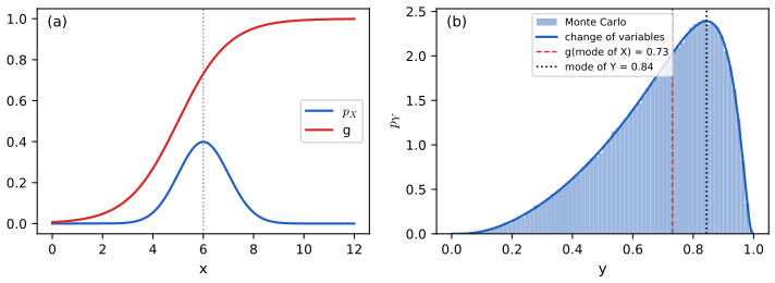
pp. 44–46 For a differentiable bijection \(\bm y=f(\bm x)\), \[ p_y(\bm y)=p_x(f^{-1}(\bm y))\,|\det\bm J_{f^{-1}}(\bm y)|,\qquad\bm J_{f^{-1}}=(\partial x_i/\partial y_j) \tag{2.257–2.258} \] (determinant = product of diagonal if triangular, 2.259). When the Jacobian is hard, use Monte Carlo \(\frac1S\sum\delta(\bm y-f(\bm x^s))\) (2.260). Figure 2.12: \(x\sim\N(6,1)\), \(y=\sigma(x-5)\); the mode of \(y\) is not the image of the mode of \(x\).
See also: first volume, Section 2.8.3; All of Statistics, Section 2.11.
Filling the gap 2.20: the change-of-variables formula, the sigmoid example, why modes are not equivariant pp. 44–45, (2.257)–(2.260)
Derivation
(2.257). With \(\bm g=f^{-1}\): \(P(\bm Y\in B)=P(\bm X\in\bm g(B))=\int_{\bm g(B)}p_x=\int_Bp_x(\bm g(\bm y))|\det\bm J_{\bm g}|\d\bm y\) (change of variables for integrals); true for all Borel \(B\), so the integrand is the density. The absolute value handles orientation reversal. Scalar: \(p_y=p_x(g(y))|g'(y)|\).
Example. \(g(y)=\operatorname{logit}y+5\), \(g'=\frac1{y(1-y)}\): \(p_Y=\N(\operatorname{logit}y+5\given6,1)/(y(1-y))\), integrating to 1 and matching the histogram.
Modes. The factor \(|g'|\) rescales the density by the stretching of space, so \(\arg\max p_Y\ne f(\arg\max p_X)\) unless \(f\) is affine: 0.844 against \(\sigma(1)=0.731\). Quantiles are equivariant for increasing \(f\), and so is the MLE; the MAP is not, so it depends on the parametrisation.
Monte Carlo. \(\frac1S\sum h(f(\bm x^s))\to\E h(f(\bm X))\) at rate \(S^{-1/2}\); the empirical measure converges weakly to the law of \(\bm Y\). No Jacobian or invertibility is needed. \(\square\)
2.5.3 Probability integral transform
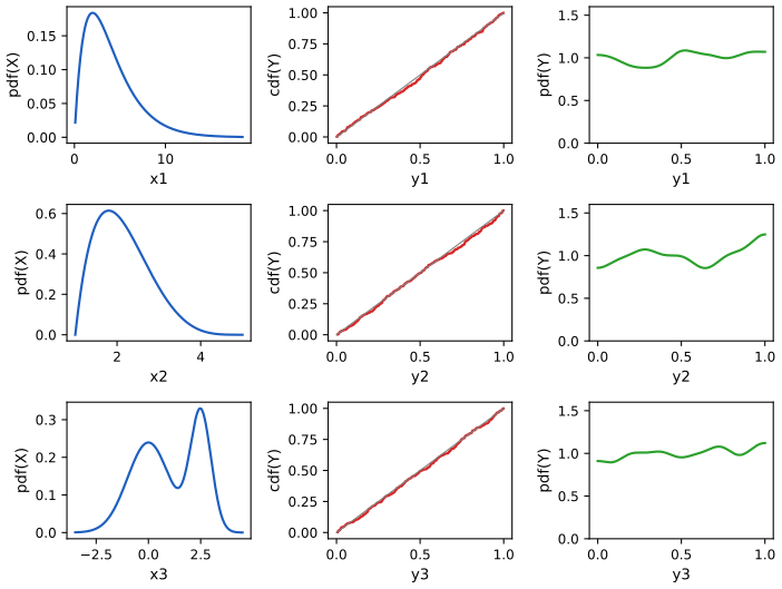
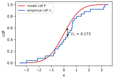
pp. 45–46 If \(X\) has cdf \(P_X\) then \(P_X(X)\sim\operatorname{Unif}(0,1)\) (2.261–2.262). Uses: sampling \(x=P_X^{-1}(u)\); testing with the Kolmogorov–Smirnov statistic \(D_n=\max_x|P_n(x)-P(x)|\) (2.263; Figure 2.14).
Filling the gap 2.21: the PIT for general cdfs, inverse-cdf sampling, and why the KS statistic is distribution-free pp. 45–46, (2.261)–(2.263)
Derivation
Quantile function. \(F^{-1}(u)=\inf\{x:F(x)\ge u\}\). Then \(F^{-1}(u)\le x\iff u\le F(x)\): if \(u\le F(x)\), \(x\) is in the set defining the infimum; conversely right-continuity gives \(F(F^{-1}(u))\ge u\), and monotonicity \(F(x)\ge u\).
Sampling. \(P(F^{-1}(U)\le x)=P(U\le F(x))=F(x)\) for every cdf, discrete or not.
PIT. The book's proof (2.261–2.262) uses \(P_X^{-1}\) as a true inverse (strictly increasing \(P_X\)). For continuous \(F\) and \(u\in(0,1)\), let \(x_u=\sup\{x:F(x)\le u\}\); \(F(x_u)=u\) and \(\{F(X)\le u\}=\{X\le x_u\}\) up to a null set, so \(P(F(X)\le u)=u\). For discrete \(X\), \(P(F(X)\le u)\le u\) (not uniform); randomise: \(U=F(X^-)+V(F(X)-F(X^-))\).
Distribution-free KS. For continuous \(F\), \(U_i=F(X_i)\) are i.i.d. uniform and \(F_n(x)=G_n(F(x))\) with \(G_n\) the empirical cdf of the \(U_i\), so \(D_n=\sup_u|G_n(u)-u|\) has a law free of \(F\). The sup is attained at a jump: \(D_n=\max_i\max\{\frac in-F(x_{(i)}),F(x_{(i)})-\frac{i-1}n\}\). Asymptotically \(\sqrt nD_n\to K\), \(P(K>t)=2\sum_{k\ge1}(-1)^{k-1}e^{-2k^2t^2}\), 5% point 1.358 (simulation at \(n=60\): 0.042); non-asymptotically \(P(D_n>\epsilon)\le2e^{-2n\epsilon^2}\) (DKW–Massart; proved in All of Statistics). Gaussian and exponential samples give indistinguishable \(D_n\) laws. Figure 2.14's 0.173 at \(n=25\) is below the 5% value 0.264: not rejected. \(\square\)
2.6 Markov chains
pp. 46–55 If \(\bm x_t\) is a sufficient statistic of the past for the future, \(p(\bm x_{t+\tau}\given\bm x_{1:t})=p(\bm x_{t+\tau}\given\bm x_t)\) (2.264), then \(p(\bm x_{1:T})=p(\bm x_1)\prod_{t\ge2}p(\bm x_t\given\bm x_{t-1})\) (2.265): a Markov chain.
See also: Bishop, Section 13.1; All of Statistics, Section 23.2.
2.6.1–2.6.3 Parameterization, language models, parameter estimation
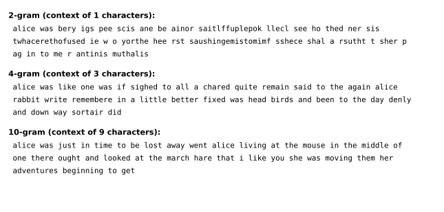
pp. 47–51 A time-invariant chain has a kernel \(p(x_t\given x_{t-1})\); for finite states, a row-stochastic matrix \(A_{ij}=p(X_t=j\given X_{t-1}=i)\) (e.g. the 2-state chain (2.266), the left-to-right chain (2.267)). The \(n\)-step matrix obeys the Chapman–Kolmogorov equations \(\bm A(m+n)=\bm A(m)\bm A(n)\), hence \(\bm A(n)=\bm A^n\) (2.268–2.271). Order-\(n\) chains (n-grams, 2.272) reduce to first order on an augmented state (2.273). Character n-gram language models generate text (Figure 2.16). The MLE from sequences is \(\hat\pi_j\propto N^1_j\), \(\hat A_{jk}=N_{jk}/N_j\) (2.274–2.278; bigram counts in Figure 2.17). With sparse data, \(\hat A_{jk}=\frac{N_{jk}+\alpha}{N_j+K\alpha}\) (2.279) (add-one for \(\alpha=1\)), which the book calls the MAP under a Dirichlet prior.
Filling the gap 2.22: Chapman–Kolmogorov, higher-order chains, the MLE, and add-\(\alpha\) smoothing is the posterior mean, not the MAP pp. 47–51, (2.265)–(2.279)
Derivation
Chapman–Kolmogorov. By total probability and the Markov property, \(P(X_{t+m+n}=j\given X_t=i)=\sum_kP(X_{t+m}=k\given X_t=i)P(X_{t+m+n}=j\given X_{t+m}=k)\) (the extra conditioning on \(X_t\) is dropped by the Markov property): \(A_{ij}(m+n)=\sum_kA_{ik}(m)A_{kj}(n)\), a matrix product; \(\bm A(n)=\bm A\bm A(n-1)\) gives \(\bm A^n\) by induction, and \(\bm\pi_n=\bm\pi_0\bm A^n\).
Higher order. For \(\tilde x_t=(x_{t-1},x_t)\) the kernel \(p(\tilde x_{t+1}\given\tilde x_t)=p(x_{t+1}\given x_{t-1},x_t)\) if the overlapping component matches and 0 otherwise: a first-order chain on \(K^n\) states, which is why \(K^{n-1}\) contexts cause sparsity.
MLE. \(\log p=\sum_jN^1_j\log\pi_j+\sum_jN_j\sum_k\frac{N_{jk}}{N_j}\log A_{jk}\) separates over rows. For a row, \(\sum_kN_{jk}\log\frac{A_{jk}}{\hat A_{jk}}\le N_j\log\sum_kA_{jk}=0\) (Jensen), so \(\hat A_{jk}=N_{jk}/N_j\); likewise \(\hat{\bm\pi}\).
Smoothing. With prior \(\bm A_{j:}\sim\Dir(\alpha\bm1)\) the posterior is \(\Dir(\bm N_{j:}+\alpha\bm1)\). Its mean is \(\frac{N_{jk}+\alpha}{N_j+K\alpha}\), which is (2.279) (Laplace's rule of succession for \(\alpha=1\)); its mode is \(\frac{N_{jk}+\alpha-1}{N_j+K(\alpha-1)}\) (gap 2.6), which for \(\alpha=1\) is the MLE: the uniform prior does nothing to the MAP. So (2.279) is the posterior mean (or the MAP under \(\Dir((\alpha+1)\bm1)\)). \(\square\)
2.6.4 Stationary distribution of a Markov chain
pp. 51–55 A distribution with \(\bm\pi=\bm\pi\bm A\) (2.280–2.282, the global balance equations) is stationary. It is found from \(\bm\pi\bm M=\bm r\) with \(\bm M=[\bm I-\bm A\text{ without its last column},\bm1]\), \(\bm r=(0,\dots,0,1)\) (2.283), or as the eigenvector of \(\bm A^\T\) for eigenvalue 1; for the chain of Figure 2.18a, \(\bm A=\begin{pmatrix}0&1&0\\\frac12&0&\frac12\\1&0&0\end{pmatrix}\), it is \((0.4,0.4,0.2)\). The 4-state chain of Figure 2.18b has two stationary distributions, \((\frac12,\frac12,0,0)\) and \((0,0,0,1)\). A limiting distribution requires irreducibility (no disconnected parts) and aperiodicity (period \(d(i)=\gcd\{t:A_{ii}(t)>0\}=1\)); then (Theorem 2.6.1) a finite irreducible aperiodic chain has a limiting distribution equal to its unique stationary distribution. For infinite state spaces one also needs recurrence and non-null states (ergodicity; Theorem 2.6.2). The detailed balance equations \(\pi_iA_{ij}=\pi_jA_{ji}\) (2.285) imply stationarity (Theorem 2.6.3). The demonstration below runs these chains. Figures 2.15 and 2.18 are diagrams of the chains and are not reproduced.
Filling the gap 2.23: existence, uniqueness and geometric convergence of the stationary distribution of a finite chain pp. 51–54, (2.280)–(2.284), Theorem 2.6.1
Derivation
Existence. The book says \(\bm A\bm1=\bm1\) gives an eigenvector, but the eigenvector of \(\bm A^\T\) for eigenvalue 1 need not be non-negative a priori. Elementary argument: for any distribution \(\bm\pi_0\) the Cesàro averages \(\bm c_n=\frac1n\sum_{t<n}\bm\pi_0\bm A^t\) lie in the compact simplex and \(\bm c_n\bm A-\bm c_n=(\bm\pi_0\bm A^n-\bm\pi_0)/n\to0\); any limit point is a stationary distribution.
Irreducible \(\Rightarrow\) positive and unique. If \(\pi_j>0\) and \(i\) is reachable from \(j\) in \(n\) steps, \(\pi_i=\sum_k\pi_kA^n_{ki}\ge\pi_jA^n_{ji}>0\): all \(\pi_i>0\). If \(\bm\pi,\bm\pi'\) are stationary, let \(c=\min_i\pi'_i/\pi_i>0\); \(\bm\pi'-c\bm\pi\ge0\) is stationary with a zero entry, so by positivity it is \(\bm0\) and \(\bm\pi'=c\bm\pi\), \(c=1\). Hence \(\operatorname{rank}(\bm I-\bm A)=K-1\), the columns of \(\bm I-\bm A\) sum to zero (so dropping the last one loses nothing), and (2.283) is a nonsingular system.
Convergence (Dobrushin). Let \(\bm B=\bm A^n>0\) (regular chain), \(m_j=\min_iB_{ij}\), \(\epsilon=\sum_jm_j>0\). For distributions \(\bm\mu,\bm\nu\), \(\bm w=\bm\mu-\bm\nu\) has \(\bm w\bm1=0\), so \(\bm w\bm B=\bm w(\bm B-\bm1\bm m^\T)\), where \(\bm B-\bm1\bm m^\T\ge0\) has row sums \(1-\epsilon\): \(\|\bm w\bm B\|_1\le(1-\epsilon)\|\bm w\|_1\). Taking \(\bm\nu=\bm\pi\) (stationary): \(\|\bm\mu\bm A^{kn}-\bm\pi\|_{TV}\le(1-\epsilon)^k\), and TV is non-increasing in \(t\): geometric convergence for every start, \(A^t_{ij}\to\pi_j\), and uniqueness. Irreducible and aperiodic imply regular: \(\{t:A_{ii}(t)>0\}\) is closed under addition with gcd 1, so contains all large integers (Schur), and irreducibility connects all pairs. The rate is governed by the second eigenvalue modulus (for two states \(|1-\alpha-\beta|\), Practice problem 2.2).
Failures. \(\alpha=\beta=1\): \(\bm A^2=\bm I\), no limit although \((\frac12,\frac12)\) is stationary. Figure 2.18b: the stationary distributions form a segment; starting in 3, the chain falls into \(\{1,2\}\) or 4 with probability \(\frac12\) each, so \(\lim\bm A^n_{3:}=(\frac14,\frac14,0,\frac12)\). (The book says the chain on \(\{1,2\}\) oscillates; with self-loops of 0.1 it is aperiodic and mixes to \((\frac12,\frac12)\).) \(\square\)
Filling the gap 2.24: detailed balance (and the typo in its proof), reversibility, and recurrence of the random walk on \(\mathbb Z\) pp. 53–55, Theorem 2.6.3, (2.285)–(2.286)
Derivation
Detailed balance. If \(\pi_iA_{ij}=\pi_jA_{ji}\) then \(\sum_i\pi_iA_{ij}=\pi_j\sum_iA_{ji}=\pi_j\), i.e. \(\bm\pi\bm A=\bm\pi\) (the book's proof ends with \(\bm\pi=\bm A\bm\pi\), wrong for the row convention). Regularity is not needed for stationarity, only for uniqueness and convergence. A stationary chain then runs backwards with the same kernel: \(P(X_t=i\given X_{t+1}=j)=\pi_iA_{ij}/\pi_j=A_{ji}\) (reversibility). The converse fails: in Figure 2.18a, \(\pi_1A_{12}=0.4\ne\pi_2A_{21}=0.2\). Detailed balance is how MCMC kernels are built (Chapter 12): choose \(\bm A\) to satisfy it for the target.
Random walk. \(A_{i,i+1}=p\), \(A_{i,i-1}=1-p=q\). \(P(S_{2n}=0)=\binom{2n}n(pq)^n\sim(4pq)^n/\sqrt{\pi n}\) (Stirling). The number of returns to 0 is geometric with mean \(f/(1-f)\) (\(f\) the return probability), so the walk is recurrent iff \(\sum_nP(S_{2n}=0)=\infty\). For \(p=\frac12\), \(\sum1/\sqrt{\pi n}\) diverges: recurrent. Otherwise \(4pq<1\), and \(\sum_{n\ge0}\binom{2n}nx^n=(1-4x)^{-1/2}\) gives expected returns \(\frac1{|1-2p|}-1\) (\(=4\) for \(p=0.6\), verified): transient. For \(p=\frac12\) the first-return generating function is \(F(s)=1-\sqrt{1-s^2}\) and the expected return time \(F'(1)=\lim s/\sqrt{1-s^2}=\infty\): null recurrent, so no stationary distribution. \(\square\)
Supplement 2.2 Google's PageRank (supplement)
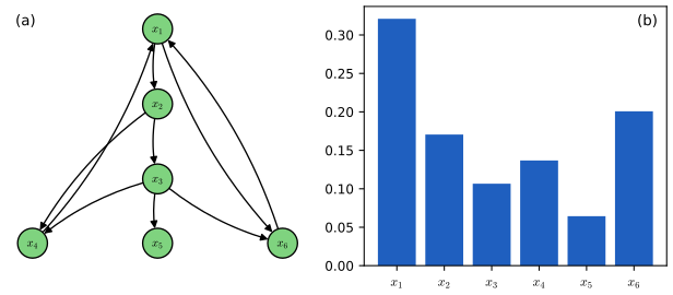
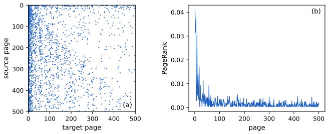
Supp. pp. 18–22 Web search retrieves pages containing the query words with an inverted index (each word stores the documents, and positions, in which it occurs; intersect the lists), then ranks by authority: \(\pi_j=\sum_iA_{ij}\pi_i\) (Supp. 2.27), the stationary distribution of a random surfer. To make the chain regular, with probability \(1-p\) the surfer jumps to a uniformly random page, giving the matrix \(M_{ij}=pG_{ij}/c_j+\delta\) if \(c_j\ne0\) and \(1/n\) otherwise (\(\delta=\frac{1-p}n\), \(c_j\) the out-degree, \(G_{ij}=1\) if \(j\to i\)), which is the rank-one perturbation \(\bm M=p\bm G\bm D+\bm1\bm z^\T\) of a sparse matrix (Supp. 2.29–2.32), and \(\bm v=\bm M\bm v\) is solved by the power method \(\bm v\leftarrow p\bm G\bm D\bm v+\bm1(\bm z^\T\bm v)\) (Supp. 2.33). For the six-page web of Figure S2.2a (links \(1\to2,6\); \(2\to3,4\); \(3\to4,5,6\); \(4\to1\); \(6\to1\); page 5 has no links) with \(p=0.85\) the stationary vector is \((0.3210,0.1705,0.1066,0.1368,0.0643,0.2007)\), within \(2\times10^{-4}\) of the book's (Supp. 2.28; the web's edges are read off the figure). Page 1 outranks pages 4 and 6 although all have one in-link: a link from an influential page counts more. Personalised PageRank (random walk with restart to page \(k\)) gives each page an importance relative to \(k\). Web spam (many links from low-rank pages) exploits the sum.
Filling the gap 2.25: the Google matrix, its rank-one form, regularity, and the convergence rate of the power method Supp. pp. 20–22, (2.27)–(2.33)
Derivation
Rank-one form. Columns of \(\bm M\) sum to 1: non-dangling \(j\): \(\sum_ipG_{ij}/c_j+n\delta=p+(1-p)=1\); dangling: \(n\cdot\frac1n\). With \(d_{jj}=1/c_j\) (0 if \(c_j=0\)) and \(z_j=\delta\) (non-dangling) or \(1/n\) (dangling), \((\bm G\bm D)_{ij}=G_{ij}/c_j\) and \(\bm M=p\bm G\bm D+\bm1\bm z^\T\) (Supp. 2.32): the sparse part is applied in \(O(\text{nnz})\) and \(\bm1\bm z^\T\bm v\) in \(O(n)\). All entries are at least \(\delta>0\), so the chain is regular and has a unique positive stationary vector (gap 2.23).
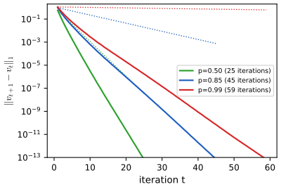
Rate. Write \(\bm M=p\tilde{\bm P}+(1-p)\frac1n\bm1\bm1^\T\) with \(\tilde{\bm P}\) the column-stochastic link matrix with dangling columns replaced by \(\frac1n\bm1\) (check columnwise). For \(\bm u=\bm v_t-\bm v\), \(\bm1^\T\bm u=0\), so \(\bm M\bm u=p\tilde{\bm P}\bm u\) and \(\|\bm M\bm u\|_1\le p\|\bm u\|_1\) (column-stochastic matrices do not increase the 1-norm): \(\|\bm v_t-\bm v\|_1\le2p^t\), and \(|\lambda_2(\bm M)|\le p\) (any eigenvector for \(\lambda\ne1\) has \(\bm1^\T\bm v=0\)). Iterations for tolerance \(\tau\): at most \(\log(\tau/2)/\log p\) (146 for \(p=0.85\), \(\tau=10^{-10}\); 41 observed on the small web). The bound is sharp for a directed cycle (its link matrix has unimodular eigenvalues): demo preset 6 contracts at exactly \(p\) per step; the simulated web is far better (Figure 2.S2). Warm starts reduce the work when the web changes.
Personalised PageRank. Restart at \(k\): \(\bm v=p\tilde{\bm P}\bm v+(1-p)\bm e_k\), so \(\bm v=(1-p)(\bm I-p\tilde{\bm P})^{-1}\bm e_k\) (the inverse exists as \(\|p\tilde{\bm P}\|_1<1\)). The Monte Carlo version counts visits of the random surfer, justified by the ergodic theorem. \(\square\)
2.7 Divergence measures between probability distributions
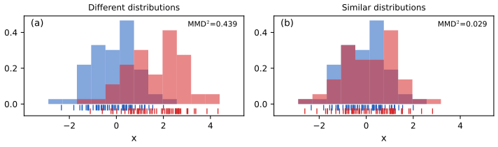
pp. 55–62 To decide whether samples \(\mathcal X\sim P\), \(\mathcal X'\sim Q\) come from the same distribution (a two-sample test, Figure 2.19) or how well a model fits data (goodness of fit), compare \(P\) and \(Q\) by a divergence: through the density ratio \(p/q\) (f-divergences) or the difference \(P-Q\) (integral probability metrics).
See also: first volume, Section 6.2 (KL divergence).
2.7.1 f-divergence
pp. 55–57 For convex \(f\) with \(f(1)=0\), \(D_f(p\|q)=\int q(x)f(p(x)/q(x))\d x\) (2.287): non-negative by Jensen, zero at \(p=q\). KL is \(f(r)=r\log r\) (2.288). The alpha divergence (Minka's form) \[ D_\alpha(p\|q)=\frac{1}{\alpha(1-\alpha)}\Big(1-\int p(x)^\alpha q(x)^{1-\alpha}\d x\Big),\qquad D^A_{\alpha'}=D^M_\alpha,\ \alpha'=2\alpha-1 \tag{2.289–2.290} \] tends to \(\KL(q\|p)\) as \(\alpha\to0\) and \(\KL(p\|q)\) as \(\alpha\to1\); \(\alpha=\frac12\) is the Hellinger case (2.291; \(f(r)=(\sqrt r-1)^2\)); \(\chi^2=\frac12\int(q-p)^2/q\) (2.293). Figure 2.20: the Gaussian \(q\) minimising \(D_\alpha(p\|q)\) for a two-component mixture \(p\) is mode-seeking for small \(\alpha\) and mass-covering for large \(\alpha\).

Filling the gap 2.26: non-negativity, the alpha family and its limits, the Hellinger metric, and why \(\alpha\) controls mode seeking pp. 55–57, (2.287)–(2.293)
Derivation
Non-negativity. Jensen: \(\int qf(p/q)\ge f(\int q\cdot p/q)=f(1)=0\). Adding \(c(r-1)\) to \(f\) does not change \(D_f\) (\(\int(p-q)=0\)).
Alpha divergence as an f-divergence. \(f(r)=\frac{1-r^\alpha}{\alpha(1-\alpha)}\) gives \(\int qf(p/q)=\frac{1-\int p^\alpha q^{1-\alpha}}{\alpha(1-\alpha)}\); it is convex for every \(\alpha\) (\(f''(r)=r^{\alpha-2}\ge0\)) with \(f(1)=0\). The Amari form (2.289) is the same with \(\alpha'=2\alpha-1\).
Limits. Put \(\alpha=1-\epsilon\): \(\int p^\alpha q^{1-\alpha}=\int pe^{\epsilon\log(q/p)}=1-\epsilon\KL(p\|q)+O(\epsilon^2)\) and \(\alpha(1-\alpha)=\epsilon(1-\epsilon)\), so \(D_\alpha\to\KL(p\|q)\). The same with \(\alpha=\epsilon\) gives \(\KL(q\|p)\).
Hellinger. \(D^M_{1/2}=4(1-\int\sqrt{pq})=2\int(\sqrt p-\sqrt q)^2=4D_H^2\) with \(D_H^2=\frac12\int(\sqrt p-\sqrt q)^2=1-\int\sqrt{pq}\) (2.291). It is the square of the metric \(D_H=\frac1{\sqrt2}\|\sqrt p-\sqrt q\|_2\) (an \(L^2\) distance, so the triangle inequality holds); the book's "squared Hellinger distance is a metric" and "\(\alpha=\frac12\) equals the Hellinger distance" hold only up to the square and the factor 4. \(\chi^2\) is \(f(r)=\frac12(r-1)^2\).
Mode seeking. \(\alpha=1\): minimising \(\KL(p\|q)\) over Gaussians \(q=\N(m,s^2)\) minimises \(\frac12\log s^2+\frac{\E_p(x-m)^2}{2s^2}\), so \(m=\E_px\) and \(s^2=\var_p\): moment matching, mass covering (\(q\) cannot be small where \(p\) has mass). For \(\alpha\ge1\) the integrand \(p^\alpha q^{1-\alpha}\) blows up where \(q\to0\) with \(p>0\): zero-avoiding. For \(\alpha\le0\) the divergence penalises \(q\) mass where \(p\) is small (\(\alpha=0\) is reverse KL): zero-forcing, and the optimum can be a local one. Numerically \(\alpha=1\) gives \((0.2000,2.3908)\) (moments of \(p\)), \(\alpha=0\) gives \((0.415,2.094)\), \(\alpha=-4\) gives \((1.985,1.015)\). \(\square\)
2.7.2–2.7.4 Integral probability metrics, MMD, total variation
pp. 57–61 An IPM is \(D_{\mathcal F}(P,Q)=\sup_{f\in\mathcal F}|\E_Pf-\E_Qf|\) (2.295), the maximiser being the witness function (Figure 2.21). With 1-Lipschitz \(f\) it is the Wasserstein-1 distance (2.296–2.297). With \(\mathcal F\) the unit ball of an RKHS it is the MMD, \(\MMD(P,Q)=\|\bm\mu_P-\bm\mu_Q\|\) (2.298–2.301), estimated by the kernel trick \[ \MMD^2(\mathcal X,\mathcal X')=\frac1{N^2}\sum_{n,n'}K(x_n,x_{n'})-\frac2{NM}\sum_{n,m}K(x_n,x'_m)+\frac1{M^2}\sum_{m,m'}K(x'_m,x'_{m'}) \tag{2.302–2.304} \] in \(O(N^2)\) time; the linear-time UME (2.305–2.306) evaluates the witness at \(J\) test locations; the bandwidth of a Gaussian kernel matters (Figure 2.22). The total variation \(\frac12\int|p-q|\) (2.307) is both an f-divergence (\(f=|r-1|/2\), 2.308) and an IPM.
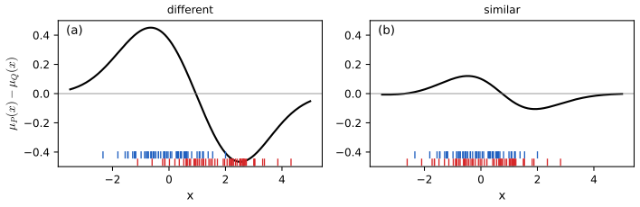
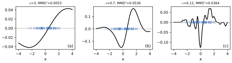
Filling the gap 2.27: total variation as a sup over events, an f-divergence and an IPM; the Wasserstein-1 dual pp. 57–61, (2.295)–(2.297), (2.307), (2.308)
Derivation
TV. For an event \(A\), \(P(A)-Q(A)=\int_A(p-q)\le\int_{p>q}(p-q)\), with equality at \(A=\{p>q\}\); since \(\int(p-q)=0\), \(\int_{p>q}(p-q)=\int_{p<q}(q-p)=\frac12\int|p-q|\). So \(\TV=\sup_A|P(A)-Q(A)|\). As an IPM: with \(\mathcal F=\{f:0\le f\le1\}\) the sup is attained at \(f=\ind_{\{p>q\}}\); with \(f=\frac12\operatorname{sign}(p-q)\) and \(\mathcal F=\{|f|\le\frac12\}\), \(\E_Pf-\E_Qf=\frac12\int|p-q|\). As an f-divergence: \(\int q\cdot\frac12|p/q-1|=\frac12\int|p-q|\) (2.308). The book cites Sriperumbudur et al. (2009) for TV being the only divergence in both classes.
Wasserstein-1. Kantorovich–Rubinstein duality: \(\inf_{\text{couplings}}\E|X-Y|=\sup_{\|f\|_L\le1}|\E_Pf-\E_Qf|\) (2.297); in one dimension both equal \(\int|F_P-F_Q|\d x\) (checked against a standard implementation). Any IPM is symmetric and satisfies the triangle inequality, and is a metric when \(\mathcal F\) separates distributions. \(\square\)
Filling the gap 2.28: the MMD: mean embeddings, the witness, the kernel trick, unbiased estimation, when MMD = 0 iff \(P=Q\), and the bandwidth limits pp. 58–60, (2.298)–(2.306)
Derivation
Mean embedding and (2.301). For a positive definite kernel \(K\) with RKHS \(\mathcal H\) and feature map \(\phi(x)=K(x,\cdot)\), \(f(x)=\langle f,\phi(x)\rangle\) (reproducing property). If \(\E\sqrt{K(x,x)}<\infty\), \(\bm\mu_P=\E_P\phi(x)\in\mathcal H\) and \(\E_Pf=\langle f,\bm\mu_P\rangle\) (a bounded linear functional). Hence \(\sup_{\|f\|\le1}\langle f,\bm\mu_P-\bm\mu_Q\rangle=\|\bm\mu_P-\bm\mu_Q\|\), attained at \(f^*=(\bm\mu_P-\bm\mu_Q)/\|\bm\mu_P-\bm\mu_Q\|\) (Cauchy–Schwarz): the witness is \(f^*(t)\propto\E_PK(x,t)-\E_QK(y,t)\), by the reproducing property.
Kernel trick. \(\|\bm\mu_P-\bm\mu_Q\|^2=\E K(x,x')+\E K(y,y')-2\E K(x,y)\); (2.304) is the plug-in (a V-statistic, biased). Dropping the diagonal terms \(n=n'\), \(m=m'\) and dividing by \(N(N-1)\), \(M(M-1)\) gives an unbiased U-statistic (checked: the average over 1500 samples is 0.1438 against the closed-form population value 0.1413, within Monte Carlo error). With explicit features the two forms agree to \(10^{-10}\) (checked with \(K=(1+xy)^2\), \(\bm\phi=(1,\sqrt2x,x^2)\)): this feature map compares only the first two moments, as the book says for \(\bm\phi=[x,x^2]\).
When \(\MMD=0\Rightarrow P=Q\). For \(K(x,y)=k(x-y)\) with \(k\) positive definite, Bochner gives \(k(u)=\int e^{i\bm\omega^\T u}\Lambda(\d\bm\omega)\) with a finite measure \(\Lambda\), and \(\MMD^2=\int|\varphi_P(\bm\omega)-\varphi_Q(\bm\omega)|^2\Lambda(\d\bm\omega)\) (\(\varphi\) the characteristic functions). The Gaussian kernel has \(\Lambda\) Gaussian with full support, so \(\MMD=0\) forces \(\varphi_P=\varphi_Q\) everywhere (continuity), hence \(P=Q\): the kernel is characteristic.
Bandwidth. \(K_\sigma=1-\frac{(x-y)^2}{2\sigma^2}+O(\sigma^{-4})\), so for \(\sigma\to\infty\), \(\MMD^2\approx(\mu_P-\mu_Q)^2/\sigma^2\): only the means; for equal means the leading term is of order \(\sigma^{-4}\) (Figure 2.22a is small). For \(\sigma\to0\), off-diagonal kernel values vanish and the V-statistic tends to \((\frac1N+\frac1M)\) (pure noise from the diagonal terms), so the test has no power: an intermediate \(\sigma\) is needed (Sutherland et al. 2017 maximise test power).
UME. \(\mu_P(v)=\E_PK(x,v)\) is estimated in \(O(N)\) per location; for analytic characteristic kernels and random \(v_j\), \(\mathrm{UME}^2>0\) almost surely if \(P\ne Q\) (Chwialkowski et al. 2015). \(\square\)
2.7.5 Density ratio estimation using binary classifiers
pp. 61–62 Label samples of \(P\) by \(y=1\) and of \(Q\) by \(y=0\), \(p(y=1)=\pi\). Bayes' rule gives \(\frac{P(x)}{Q(x)}=\frac{p(y=1\given x)}{p(y=0\given x)}\frac{1-\pi}\pi\) (2.309–2.310): with \(\pi=\frac12\), a classifier \(h(x)=p(y=1\given x)\) gives \(r=h/(1-h)\). Minimising the log-loss risk \(\pi\E_P[-\log h]+(1-\pi)\E_Q[-\log(1-h)]\) (2.311–2.312), or another loss, yields a divergence: Nguyen, Wainwright and Jordan (2009) show each f-divergence has a loss with \(-D_f=R^*_{\ell}\). The book pairs TV with hinge loss, Hellinger with exponential loss and \(\chi^2\) with logistic loss; and shows that \(\ell=-2\tilde yh\) gives the IPM (2.313–2.316).
Filling the gap 2.29: the Bayes-optimal classifier and the loss–divergence correspondence (and the correct partner of the logistic loss) pp. 61–62, (2.309)–(2.316)
Derivation
Ratio. \(\frac{p(y=1\given x)}{p(y=0\given x)}=\frac{P(x)\pi}{Q(x)(1-\pi)}\), rearranged. The risk is minimised pointwise: for each \(x\) minimise \(-\pi P(x)\log h-(1-\pi)Q(x)\log(1-h)\); by Gibbs' inequality, \(h^*=\frac{\pi P}{\pi P+(1-\pi)Q}\), the true posterior.
Bayes risks at \(\pi=\frac12\) (margin form \(\tilde y\in\{\pm1\}\), risk \(\frac12\E_P\ell(+1,h)+\frac12\E_Q\ell(-1,h)\), minimised pointwise over the score \(h\); integrals are \(\int\)\(\d x\)). Hinge \(\max(0,1-\tilde yh)\): the optimum is \(h=\pm1\), pointwise value \(\min(p,q)\), so \(R^*=\int\min(p,q)=1-\TV\). Exponential \(e^{-\tilde yh}\): \(\frac12(pe^{-h}+qe^h)\) is minimised at \(e^{2h}=p/q\) with value \(\sqrt{pq}\), so \(R^*=\int\sqrt{pq}=1-D_H^2\). Logistic \(\log(1+e^{-\tilde yh})\): optimum \(e^h=p/q\), value \(\frac12[p\log\frac{p+q}p+q\log\frac{p+q}q]\), so \(R^*=\log2-\JS(P,Q)\), with \(\JS=\frac12\KL(P\|M)+\frac12\KL(Q\|M)\), \(M=\frac{P+Q}2\) (the same as the cross-entropy risk, since \(-\log h^*=-\log\frac{p}{p+q}=-\log\frac p{M}+\log2\)). Square \((1-\tilde yh)^2\): optimum \(h=\frac{p-q}{p+q}\), value \(\frac{2pq}{p+q}\), so \(R^*=1-\frac12\int\frac{(p-q)^2}{p+q}\), the triangular discrimination (a symmetrised \(\chi^2\)). So TV, Hellinger and Jensen–Shannon (the GAN objective) go with hinge, exponential and logistic losses, and a \(\chi^2\)-type divergence with the square loss; the book's "\(\chi^2\) corresponds to logistic loss" is not right. Also \(-D_f=R^*\) holds up to an additive constant and scale. All five were confirmed by numerical integration for \(P=\N(0,1)\), \(Q=\N(1.3,1.4^2)\) (e.g. log-loss risk 0.552074 \(=\log2-\JS\)).
The IPM case. With \(\ell(\tilde y,h)=-2\tilde yh\) and \(\pi=\frac12\), \(R(h)=\E_Qh-\E_Ph\) (2.315); the infimum over \(h\) is \(-\sup_h(\E_Ph-\E_Qh)\), which is \(-\infty\) unless \(h\) ranges over a bounded class (Lipschitz functions, an RKHS ball): the classifier is the witness function of an IPM for that class. \(\square\)
2.8 Practice problems
The book has no exercises for Chapter 2; these three short problems practise the new material (each solution is worked independently and checked numerically).
Problem 2.1 (negative binomial as a gamma-Poisson mixture). Let \(\lambda\sim\Ga(r,\text{scale }\frac p{1-p})\) and \(X\given\lambda\sim\Poi(\lambda)\). Show that \(X\sim\operatorname{NegBinom}(r,p)\), and that \(\var X=\E X+(\E X)^2/r\). What happens as \(r\to\infty\) with the mean fixed?
Solution
\(p(x)=\int_0^\infty\frac{e^{-\lambda}\lambda^x}{x!}\frac{\lambda^{r-1}e^{-\lambda(1-p)/p}}{\Gamma(r)\theta^r}\d\lambda\) with \(\theta=\frac p{1-p}\). The exponent is \(e^{-\lambda(1+1/\theta)}=e^{-\lambda/p}\) since \(1+\frac{1-p}p=\frac1p\), and \(\int\lambda^{x+r-1}e^{-\lambda/p}\d\lambda=\Gamma(x+r)p^{x+r}\). So \(p(x)=\frac{\Gamma(x+r)p^{x+r}}{x!\Gamma(r)\theta^r}=\frac{\Gamma(x+r)}{x!\Gamma(r)}p^x(1-p)^r\), which is (2.25). Law of total variance: \(\var X=\E[\lambda]+\var[\lambda]=r\theta+r\theta^2\) and \(\E X=r\theta\), so \(\var X=\E X+(\E X)^2/r\). With \(\E X=m=r\theta\) fixed, \(\var\lambda=m^2/r\to0\): the rate becomes deterministic and \(X\to\Poi(m)\), the Poisson limit of gap 2.2. (Checked numerically for \(r=4\), \(p=0.3\).) \(\square\)
Problem 2.2 (the two-state chain). For \(\bm A=\begin{pmatrix}1-\alpha&\alpha\\\beta&1-\beta\end{pmatrix}\) with \(\alpha+\beta>0\), find the stationary distribution, a closed form for \(\bm A^n\), and the rate of convergence. What happens for \(\alpha=\beta=1\) and \(\alpha=\beta=0\)?
Solution
Global balance: \(\pi_1\alpha=\pi_2\beta\), with \(\pi_1+\pi_2=1\): \(\bm\pi=\frac1{\alpha+\beta}(\beta,\alpha)\). The eigenvalues are 1 and \(\lambda=1-\alpha-\beta\) (the trace is \(2-\alpha-\beta\)). Write \(\bm\Pi=\bm1\bm\pi\) (both rows \(\bm\pi\)); then \(\bm\Pi^2=\bm\Pi\) and \(\bm\Pi\bm A=\bm A\bm\Pi=\bm\Pi\) (stationarity and \(\bm A\bm1=\bm1\)). A direct check of the four entries (e.g. \(A_{11}-\Pi_{11}=1-\alpha-\frac\beta{\alpha+\beta}=\frac{\alpha(1-\alpha-\beta)}{\alpha+\beta}=\lambda(1-\Pi_{11})\)) shows \(\bm A-\bm\Pi=\lambda(\bm I-\bm\Pi)\). Since \(\bm I-\bm\Pi\) is a projection and \(\bm\Pi(\bm I-\bm\Pi)=\bm0\), \(\bm A^n=\bm\Pi+\lambda^n(\bm I-\bm\Pi)\). Hence \(\bm\pi_0\bm A^n-\bm\pi=\lambda^n(\bm\pi_0-\bm\pi)\): the total variation distance decays exactly as \(|1-\alpha-\beta|^n\) (demo preset 1: \(0.6^n\)). For \(\alpha=\beta=1\), \(\lambda=-1\): the chain alternates, \(\bm A^n\) does not converge (it is periodic) though \((\frac12,\frac12)\) is stationary. For \(\alpha=\beta=0\), \(\bm A=\bm I\): reducible, every distribution is stationary. (Checked for \(\alpha=0.3,\beta=0.1\) at \(n=9\).) \(\square\)
Problem 2.3 (when is the exact sensor-fusion posterior bimodal?). Two devices give \(N_x=N_y=2\) readings with the same sample standard deviation \(s\) and means \(\bar x,\bar y\). Show that the posterior \(\propto[((\bar x-z)^2+s^2)((\bar y-z)^2+s^2)]^{-1}\) has two modes iff \(|\bar x-\bar y|>2s\), and give them. For the book's means (1.5, 3.5) what is the largest \(s\) for which the posterior is bimodal?
Solution
This is the computation at the end of gap 2.14: with \(u=z-\frac{\bar x+\bar y}2\), \(a=\frac{|\bar x-\bar y|}2\), the reciprocal is \(g(u)=(u^2+a^2+s^2)^2-4a^2u^2\); as a function of \(w=u^2\) its derivative \(2(w+a^2+s^2)-4a^2\) vanishes at \(w=a^2-s^2\). If \(a>s\) then \(g\) has minima at \(u=\pm\sqrt{a^2-s^2}\) (modes of the posterior) and a local maximum at \(u=0\); if \(a\le s\) the single stationary point is \(u=0\). So bimodal iff \(|\bar x-\bar y|>2s\), with modes at \(\frac{\bar x+\bar y}2\pm\sqrt{a^2-s^2}\). For means 1.5 and 3.5, \(a=1\): bimodal iff \(s<1\); at \(s=0.4\) the modes are \(2.5\pm0.917=1.58,3.42\). (Confirmed by the demonstration: preset 3.) \(\square\)
Demonstrations
| Page | What it shows | In the notes |
|---|---|---|
| Sensor fusion with unknown noise | Two devices with unknown precisions: the plug-in Gaussian (maximum likelihood precisions) against the exact bimodal posterior, with sliders for the means, spreads and numbers of readings. Presets: 1 book's data; 2 agreeing; 3 symmetric disagreement; 4 ten readings; 5 noisy device. | Supp. 2.1.2, gap 2.14 |
| Alpha divergence | The Gaussian minimising \(D_\alpha(p\|q)\) to a two-mode mixture as \(\alpha\) moves from \(-4\) to \(4\). Presets: 1 \(\alpha=1\); 2 \(\alpha=0\); 3 \(\alpha=\frac12\); 4 \(\alpha=-4\); 5 \(\alpha=4\), wide gap. | 2.7.1, gap 2.26 |
| Markov chains and PageRank | Distribution after \(t\) steps and the total-variation error for two-state, three-state and reducible chains and PageRank on a small web, a 500-page web and a cycle. Presets: 1 two states; 2 periodic; 3 Figure 2.18a; 4 Figure 2.18b; 5 small web; 6 cycle. | 2.6.4, Supp. 2.2, gap 2.23, gap 2.25 |
The Python code that produces every figure of this page is code/ch02_probability.py (see the code index).
Notes on the book
Points where the book is imprecise or wrong
- Poisson limit of the negative binomial (Section 2.2.1.4). \(\operatorname{NegBinom}(r,\frac\lambda{1+\lambda})\) has mean \(r\lambda\); the limit needs \(p=\frac\lambda{r+\lambda}\) (gap 2.2).
- (2.50) The multivariate Student normaliser has \(|\bm\Sigma|^{+1/2}\), not \(-1/2\) (gap 2.3).
- (2.60) and (2.64) The Wishart normaliser is \(|\bm S|^{+\nu/2}2^{\nu D/2}\Gamma_D(\nu/2)\) and the inverse Wishart's is \(|\bm S|^{-\nu/2}2^{\nu D/2}\Gamma_D(\nu/2)\); the book has the opposite signs. (2.62): with the scale convention of (2.59), \(\Wi(\lambda\given s,\nu)=\Ga(\frac\nu2,\frac1{2s})\) and the chi-squared case is \(s=1\), not \(s=2\) (gap 2.7).
- Gaussian shells, before (2.74). \(\var[x_i^2]=2\), so \(\var d^2=2D\) and the coefficient of variation is \(\sqrt{2/D}\); the radial thickness of the shell is \(O(\sigma)\), not \(O(\sigma D^{1/4})\) (gap 2.9).
- (2.84)–(2.85) versus Section 2.3.1.6. The text says the section derives (2.85) and (2.86); it derives the conditional (2.86) and the marginal (2.116)–(2.117). Section 2.3.1.5 derives only the conditional, not the marginal (2.77) it is cited for (gap 2.10).
- (2.153) The scalar CPD potential has \(1/\sigma^2\), not \(1/\sigma\) (gap 2.12). (2.196) keeps a stray \(\sigma\) (\(A=\mu^2/2\) for unit variance).
- (2.238) and (2.240). The conjugate is \(\sup_{\bm\eta}\bm m^\T\bm\eta-A(\bm\eta)\) (the text writes \(\bm\mu\)), and the Bregman divergence of the conjugate uses \(A^*\), not \(A\) (gap 2.17).
- Hellinger (2.291). The (squared) Hellinger quantity is not itself a metric (its square root is), and the Minka alpha divergence at \(\alpha=\frac12\) is \(4D_H^2\), not \(D_H\) (gap 2.26).
- Theorem 2.6.3. The proof ends with \(\bm\pi=\bm A\bm\pi\); with the row convention it is \(\bm\pi\bm A=\bm\pi\). Regularity is not needed for \(\bm\pi\) to be stationary (gap 2.24).
- (2.279). \(\frac{N_{jk}+\alpha}{N_j+K\alpha}\) is the posterior mean under \(\Dir(\alpha\bm1)\) (Laplace's rule for \(\alpha=1\)); the MAP under that prior is \(\frac{N_{jk}+\alpha-1}{N_j+K(\alpha-1)}\), which for \(\alpha=1\) is the MLE (gap 2.22).
- Figure 2.18b discussion. With self-transition 0.1 the chain on \(\{1,2\}\) is aperiodic and does not oscillate; \((0.5,0.5,0,0)\) is the limit, not a cycle (gap 2.23).
- Section 2.7.5. The minimum logistic-loss risk is \(\log2-\JS(P,Q)\) (Jensen–Shannon), not a \(\chi^2\) divergence; the \(\chi^2\)-type partner is the square loss (gap 2.29). The IPM derivation (2.313)–(2.316) needs a bounded function class.
- Section 2.5.3, PIT. The proof assumes an invertible cdf; for general continuous \(P_X\) and for discrete variables see gap 2.21.
References
- Murphy, K. P. (2023). Probabilistic Machine Learning: Advanced Topics. MIT Press, Cambridge, MA. Chapter 2 and Supplementary Chapter 2. probml.github.io/pml-book/book2.html.
- Barndorff-Nielsen, O. (1978). Information and Exponential Families in Statistical Theory. Wiley, Chichester.
- Chwialkowski, K., Ramdas, A., Sejdinovic, D. and Gretton, A. (2015). Fast two-sample testing with analytic representations of probability measures. Advances in Neural Information Processing Systems, 28.
- Darmois, G. (1935). Sur les lois de probabilité à estimation exhaustive. Comptes Rendus de l'Académie des Sciences, 200, 1265–1266.
- Gretton, A., Borgwardt, K. M., Rasch, M. J., Schölkopf, B. and Smola, A. (2012). A kernel two-sample test. Journal of Machine Learning Research, 13, 723–773.
- Haveliwala, T. and Kamvar, S. (2003). The second eigenvalue of the Google matrix. Stanford technical report.
- Koopman, B. O. (1936). On distributions admitting a sufficient statistic. Transactions of the American Mathematical Society, 39, 399–409.
- Laurent, B. and Massart, P. (2000). Adaptive estimation of a quadratic functional by model selection. Annals of Statistics, 28(5), 1302–1338.
- Minka, T. (2005). Divergence measures and message passing. Microsoft Research technical report MSR-TR-2005-173.
- Muirhead, R. J. (1982). Aspects of Multivariate Statistical Theory. Wiley, New York.
- Nguyen, X., Wainwright, M. J. and Jordan, M. I. (2009). On surrogate loss functions and f-divergences. Annals of Statistics, 37(2), 876–904.
- Pitman, E. J. G. (1936). Sufficient statistics and intrinsic accuracy. Proceedings of the Cambridge Philosophical Society, 32, 567–579.
- Sriperumbudur, B. K., Fukumizu, K., Gretton, A., Schölkopf, B. and Lanckriet, G. (2009). On integral probability metrics, \(\phi\)-divergences and binary classification. arXiv:0901.2698.
- Sutherland, D. J., Tung, H.-Y., Strathmann, H., De, S., Ramdas, A., Smola, A. and Gretton, A. (2017). Generative models and model criticism via optimized maximum mean discrepancy. ICLR.
The numerical statements in the text (the density and moment formulas, the Wishart and Student normalisers, the Gaussian shell, the marginals, conditionals and potentials, the linear Gaussian system, the sensor-fusion numbers, the exponential-family identities, the change of variables and PIT, the stationary distributions, the PageRank vector, the alpha-divergence fits, the MMD identities, the loss-divergence correspondence and the answers to the practice problems) were confirmed numerically.