Monte Carlo methods
Monte Carlo replaces an integral by an average over random draws, and its error shrinks like \(1/\sqrt{N}\) whatever the dimension. This chapter, the first of three on sampling, builds the toolbox: how to draw from simple distributions (inverse cdf, polar Box-Muller), how to draw from an unnormalised target by rejection (and why that fails in high dimension), how to reweight draws from the wrong distribution (importance sampling, its self-normalised form and annealed importance sampling for normalising constants), and five ways to cut the variance (common random numbers, Rao-Blackwellisation, control variates, antithetic draws and quasi-Monte Carlo). The notes prove each result the book states without proof, check its numerical examples, and reproduce the computed figures with my own code.
Ch. 1 Introduction Ch. 2 Probability Ch. 3 Statistics Ch. 4 Graphical models Ch. 5 Information theory Ch. 6 Optimisation Ch. 7 Inference algorithms Ch. 8 Gaussian filtering Ch. 9 Message passing Ch. 10 Variational inference Ch. 11 Monte Carlo Ch. 12 MCMC Ch. 13 Sequential Monte Carlo Ch. 14 Predictive models Ch. 15 GLMs Ch. 16 Deep networks Ch. 17 Bayesian neural networks Ch. 18 Gaussian processes Ch. 19 Beyond iid Ch. 20 Generative models Ch. 21 VAEs Ch. 22 Autoregressive models Ch. 23 Normalizing flows Ch. 24 Energy-based models Ch. 25 Diffusion models Ch. 26 GANs Ch. 27 Discovery methods Ch. 28 Latent factor models Ch. 29 State-space models Ch. 30 Graph learning Ch. 31 Nonparametric Bayes Ch. 32 Representation learning Ch. 33 Interpretability Ch. 34 Decision making Ch. 35 Reinforcement learning Ch. 36 Causality
How to read these notes
They follow the book. Sections carry the book's numbers. The draft numbers many equations of this chapter, and I keep those numbers where I restate them, e.g. (11.7), (11.28), (11.58). The chapter is short, and its proofs are mostly sketched or omitted, so most of the work here is in the gap boxes.
Filling the gaps. Wherever the book states a result without proof (the standard error, the correctness of the Box-Muller and adaptive rejection samplers, the bias of self-normalised importance sampling, the validity of annealed importance sampling, the optimal control-variate coefficient, the rate of quasi-Monte Carlo), an orange Filling the gap box gives the full argument. Proofs start hidden.
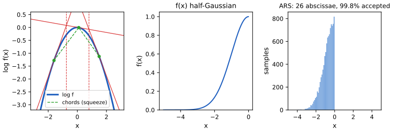
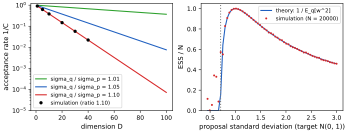
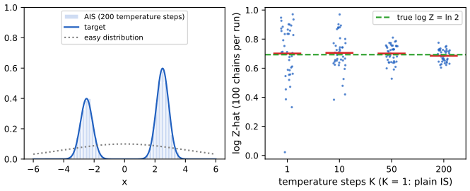
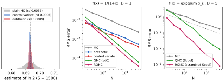
Figures. Figures 11.1 to 11.5 and 11.7 are reproduced from simulation with my own samplers (the adaptive rejection sampler, the polar method, the gamma rejection sampler, the Sobol point sets). Figures 11.4a and 11.6 are hand-drawn schematics and are not reproduced. Figures 11.8 to 11.10 are my own, for the topics the book only describes (annealed importance sampling, the high-dimensional behaviour of rejection and importance sampling, and the variance-reduction methods compared).
Main reference
K. P. Murphy, Probabilistic Machine Learning: Advanced Topics, MIT Press (2023; December 2025 draft), Chapter 11, pages 483–498 (book page: probml.github.io/pml-book/book2.html). The explanations, derivations, figures and code are my own.
Companion courses
- All of Statistics: 24.2 basic Monte Carlo integration and 24.3 importance sampling prove the unbiasedness, the \(1/\sqrt N\) rate, the optimal proposal and the effective sample size in the form used here.
- Bayesian and Probabilistic Machine Learning: Chapter 11 (sampling methods) proves inverse-cdf sampling, the polar Box-Muller method, rejection sampling and adaptive rejection sampling, and the exponential decay of the acceptance rate with dimension.
- Probabilistic Machine Learning: An Introduction: Chapter 2 (Monte Carlo approximation of expectations, Result 2.20).
- This course: 7.4.5 MCMC and 7.4.6 sequential Monte Carlo place these methods among the inference algorithms; gap 6.3 uses control variates and Rao-Blackwellisation on the score-function gradient estimator. Chapter 12 (MCMC) and Chapter 13 (sequential Monte Carlo) continue from here.
What this chapter adds: the sharp form of every constant (the gamma envelope and its optimal proposal rate, the effective sample size of a Gaussian proposal, the variance of control-variate and antithetic estimators for the book's worked example), a complete proof that annealed importance sampling is unbiased, and quasi-Monte Carlo with its limits.
The chapter at a glance
- 11.2 \(\E[f(x)]\approx\frac1{N}\sum_nf(x_n)\): unbiased, variance \(\sigma^2/N\), a confidence interval and a sample-size rule (gap 11.1).
- 11.3 The inverse-cdf transform (gap 11.2) and the polar Box-Muller method (gap 11.3).
- 11.4 Rejection sampling (gap 11.4), the gamma example and its optimal proposal (gap 11.5), adaptive rejection sampling (gap 11.6), and why it fails in high dimension (gap 11.7).
- 11.5 Importance sampling, direct and self-normalised (gap 11.8), the choice of proposal (gap 11.9) and annealed importance sampling (gap 11.10).
- 11.6 Variance reduction: common random numbers (gap 11.11), Rao-Blackwellisation (gap 11.12), control variates (gap 11.13), antithetic sampling (gap 11.14) and quasi-Monte Carlo (gap 11.15).
Notation. \(p(x)\) is the target, \(\tilde p\) or \(\tilde\gamma\) its unnormalised version, \(q\) a proposal, \(N_s\) or \(N\) the number of draws, \(\mu=\E[f(X)]\), \(\sigma^2=\var[f(X)]\), \(\tilde w_n\) unnormalised and \(W_n\) normalised importance weights.
11.1 Introduction
p. 483 Monte Carlo (MC) methods solve numerical integration problems by random sampling. This chapter gives the key ideas; MCMC (Chapter 12) and sequential Monte Carlo (Chapter 13) build on them. In the Bayesian setting the target is usually a posterior \(p(x\given y)\) known only up to its normalising constant, \(\tilde p(x)=p(x,y)\) with \(Z=p(y)=\int p(x,y)\d x\), so most of what follows works with unnormalised densities. For further reading the book cites Liu (2001), Robert and Casella (2004) and Kroese, Taimre and Botev (2011).
11.2 Monte Carlo integration
p. 483 The task is the expectation \[ \E[f(x)]=\int f(x)p(x)\d x,\qquad x\in\R^n,\ f:\R^n\to\R^m, \tag{11.1} \] which a grid (quadrature in 1-D, cubature in higher dimension) can do well only up to about three dimensions, because a grid with \(m\) points per axis needs \(m^D\) evaluations. Monte Carlo instead draws \(x_n\sim p\) and averages: \[ \E[f(x)]\approx\frac1{N_s}\sum_{n=1}^{N_s}f(x_n). \tag{11.2} \] It evaluates \(f\) only where \(p\) has mass, and its accuracy depends on \(N_s\) and on \(\var[f]\), not on the dimension of \(x\) (gap 11.1). The catch is that one must be able to draw from \(p\), and that \(\var[f]\) can be large, which is what the rest of the chapter addresses.
11.2.1 Example: estimating π by Monte Carlo integration
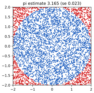
p. 484 The area of the disc of radius \(r\) is \(\pi r^2=\iint\ind(x^2+y^2\le r^2)\d x\d y\). With \(x,y\sim\Unif(-r,r)\) independent, so \(p(x)p(y)=1/(2r)^2\), \[ I=4r^2\iint f(x,y)p(x)p(y)\d x\d y\approx4r^2\frac1{N_s}\sum_{n=1}^{N_s}f(x_n,y_n),\qquad f=\ind(x^2+y^2\le r^2), \tag{11.3--11.6} \] and \(\hat\pi=\hat I/r^2=4\hat p\), where \(\hat p\) is the fraction of points inside the disc. The indicator is Bernoulli with success probability \(\pi/4\), so \(\operatorname{se}(\hat\pi)=\sqrt{\pi(4-\pi)/N_s}\) (gap 11.1). With \(N_s=5000\) this is \(0.0232\): my run with \(r=2\) and seed 0 gives \(\hat\pi=3.165\), \(\operatorname{se}=0.023\). The book quotes \(\hat\pi=3.10\) with standard error \(0.09\); the number \(0.09\) is the standard error of the area estimate \(\hat I\) (it is \(r^2=4\) times larger), not of \(\hat\pi\) (Notes on the book, item 1).
11.2.2 Accuracy of Monte Carlo integration
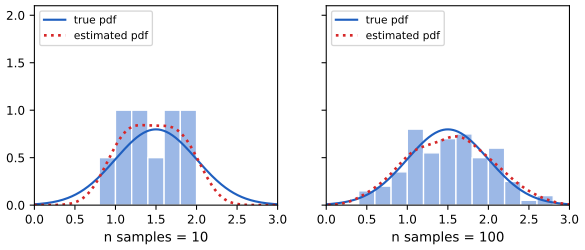
p. 484–485 Write \(\mu=\E[f(X)]\), \(\hat\mu\) for the average (11.2) and \(\sigma^2=\var[f(X)]=\E[f^2]-\E[f]^2\) (11.8). For independent draws, \[ \hat\mu-\mu\ \to\ \N\!\Big(0,\frac{\sigma^2}{N_s}\Big)\quad\text{(in the sense of the central limit theorem)}, \tag{11.7} \] \[ \hat\sigma^2=\frac1{N_s}\sum_n\big(f(x_n)-\hat\mu\big)^2,\qquad P\Big(\hat\mu-1.96\frac{\hat\sigma}{\sqrt{N_s}}\le\mu\le\hat\mu+1.96\frac{\hat\sigma}{\sqrt{N_s}}\Big)\approx0.95. \tag{11.9, 11.10} \] The quantity \(\hat\sigma/\sqrt{N_s}\) is the (numerical) standard error. To be within \(\pm\epsilon\) with probability about 95%, take \(N_s\ge(1.96)^2\hat\sigma^2/\epsilon^2\approx4\hat\sigma^2/\epsilon^2\). The error \(\sigma/\sqrt{N_s}\) does not depend on the dimension of the integral; what does depend on it is whether one can sample from \(p\) and how big \(\sigma^2\) is (gap 11.1).
Filling the gap 11.1: unbiasedness, variance, the confidence interval and the sample-size rule pp. 484–485
Derivation
Let \(X_1,\dots,X_N\) be i.i.d. from \(p\), \(Y_n=f(X_n)\) with \(\E|Y|<\infty\), and \(\hat\mu=\frac1N\sum_nY_n\).
Unbiased. \(\E\hat\mu=\frac1N\sum_n\E Y_n=\mu\) by linearity (no independence needed).
Variance. If \(\sigma^2<\infty\), then \(\var\hat\mu=\frac1{N^2}\big(\sum_n\var Y_n+\sum_{n\ne m}\cov(Y_n,Y_m)\big)=\sigma^2/N\), since independent variables are uncorrelated. In particular \(\hat\mu\to\mu\) in mean square, and almost surely by the strong law of large numbers. Nothing here involves \(\dim x\): the dimension enters only through \(\sigma^2\) and through the difficulty of sampling.
Confidence interval. By the central limit theorem \(\sqrt N(\hat\mu-\mu)/\sigma\to\N(0,1)\) in distribution. The plug-in (11.9) satisfies \(\hat\sigma^2=\frac1N\sum Y_n^2-\hat\mu^2\to\E Y^2-\mu^2=\sigma^2\) almost surely (law of large numbers applied to \(Y^2\) and to \(Y\), plus continuity), so by Slutsky's lemma \(\sqrt N(\hat\mu-\mu)/\hat\sigma\to\N(0,1)\). Since \(\Pr(|Z|\le1.96)=0.95\) for \(Z\sim\N(0,1)\), the interval \(\hat\mu\pm1.96\hat\sigma/\sqrt N\) covers \(\mu\) with probability tending to 0.95, which is (11.10). (Dividing by \(N-1\) instead of \(N\) in (11.9) makes \(\hat\sigma^2\) unbiased and changes nothing asymptotically.)
Sample size. The half-width \(1.96\hat\sigma/\sqrt N\) is at most \(\epsilon\) iff \(N\ge1.96^2\hat\sigma^2/\epsilon^2\), and \(1.96^2=3.84\le4\), so \(N\ge4\hat\sigma^2/\epsilon^2\) suffices. A non-asymptotic guarantee needs more: by Chebyshev, \(\Pr(|\hat\mu-\mu|\ge\epsilon)\le\sigma^2/(N\epsilon^2)\le0.05\) once \(N\ge20\sigma^2/\epsilon^2\); and if \(f\in[a,b]\), Hoeffding's inequality gives \(\Pr(|\hat\mu-\mu|\ge\epsilon)\le2e^{-2N\epsilon^2/(b-a)^2}\), so \(N\ge\frac{(b-a)^2}{2\epsilon^2}\ln40\) suffices.
The estimate of \(\pi\). With \(f=\ind(\text{disc})\) and uniform points on the square, \(f\) is Bernoulli\((p)\) with \(p=\pi r^2/(2r)^2=\pi/4\). Then \(\hat\pi=4\hat p\) and \(\var\hat\pi=16\,p(1-p)/N=\pi(4-\pi)/N\), so \(\operatorname{se}(\hat\pi)=\sqrt{\pi(4-\pi)/5000}=0.0232\). The area estimate \(\hat I=r^2\hat\pi\) has standard error \(r^2\cdot0.0232=0.093\) for \(r=2\). A sample size for \(\pm0.01\) at 95% is \(N\ge4\cdot\pi(4-\pi)/10^{-4}\approx1.08\times10^5\).
See also: All of Statistics, gap 24.2 (the proof and the dimension-free rate); Introduction volume, Chapter 2.
11.3 Generating random samples from simple distributions
p. 486 The main computational task is to draw from the target \(p^*(x)\) (often a posterior). This section gives exact methods for simple univariate distributions; they are the building blocks for the multivariate ones.
11.3.1 Sampling using the inverse cdf
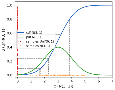
pp. 486–487 Theorem 11.3.1. If \(U\sim\Unif(0,1)\) and \(F\) is a cdf with inverse \(F^{-1}\), then \(F^{-1}(U)\sim F\). The book's proof applies \(F\) to both sides of \(F^{-1}(U)\le x\), which needs \(F\) strictly increasing and continuous; gap 11.2 proves it for every cdf by using the generalised inverse. For the exponential distribution \(F(x)=1-e^{-\lambda x}\) on \(x\ge0\), so \(F^{-1}(p)=-\ln(1-p)/\lambda\) (11.15), and because \(1-U\sim\Unif(0,1)\) as well, \(-\ln(U)/\lambda\) also works. Figure 11.3 shows the construction for \(\N(3,1)\): a height \(u\) on the vertical axis is slid across to the cdf and dropped to the \(x\) axis.
Filling the gap 11.2: the inverse-cdf theorem for an arbitrary cdf p. 486
Derivation
For a general cdf \(F\) (nondecreasing, right-continuous, with limits 0 and 1) define the generalised inverse \(F^{-1}(u)=\inf\{x:F(x)\ge u\}\) for \(u\in(0,1)\); the set is non-empty and bounded below. Claim: \(F^{-1}(u)\le x\iff u\le F(x)\).
(\(\Leftarrow\)) If \(u\le F(x)\) then \(x\) is in the set, so the infimum is at most \(x\). (\(\Rightarrow\)) Let \(x_0=F^{-1}(u)\). Choose \(x_k\downarrow x_0\) in the set, so \(F(x_k)\ge u\); right-continuity gives \(F(x_0)=\lim F(x_k)\ge u\), i.e. the infimum is attained. If \(x_0\le x\) then \(F(x)\ge F(x_0)\ge u\) by monotonicity.
Hence \(\Pr(F^{-1}(U)\le x)=\Pr(U\le F(x))=F(x)\), because \(\Pr(U\le y)=y\) on \([0,1]\). This holds for discrete and mixed distributions too: for a Bernoulli\((p)\), \(F^{-1}(u)=\ind(u>1-p)\), the familiar "compare \(u\) with the cumulative probabilities".
Exponential. \(F(x)=1-e^{-\lambda x}\) is continuous and strictly increasing on \([0,\infty)\); solving \(F(x)=u\) gives \(x=-\ln(1-u)/\lambda\). Since \(U\) and \(1-U\) have the same law, \(-\ln(U)/\lambda\) is also \(\Expon(\lambda)\) with mean \(1/\lambda\).
See also: Bayesian and Probabilistic ML, Result 11.3 (inverse distribution function method).
11.3.2 Sampling from a Gaussian (Box-Muller method)
p. 487 Draw \(z_1,z_2\sim\Unif(-1,1)\), keep the pair only if \(r^2=z_1^2+z_2^2\le1\) (so \(z\) is uniform on the unit disc), and set
\[ x_i=z_i\Big(\frac{-2\ln r^2}{r^2}\Big)^{1/2},\qquad i=1,2. \tag{11.16} \]
Then \(x_1,x_2\) are independent \(\N(0,1)\) draws (11.17); this is the polar form of the Box-Muller method (gap 11.3). For \(\N(\mu,\Sigma)\), factor \(\Sigma=LL^\T\) (Cholesky), draw \(x\sim\N(0,I)\) and set \(y=Lx+\mu\); then \(\cov[y]=L\,I\,L^\T=\Sigma\) (11.18). My code implements both (box_muller_polar, mvn_sample).
Filling the gap 11.3: why the polar method gives independent Gaussians, and its cost p. 487
Derivation
Rejection from the square keeps points uniform on the disc, with density \(1/\pi\). Write \(z=(\rho\cos\Theta,\rho\sin\Theta)\). The Jacobian of polar coordinates is \(\rho\), so \((\rho,\Theta)\) has density \(\rho/\pi\) on \((0,1)\times(0,2\pi)\): it factorises, so \(\rho\) and \(\Theta\) are independent, \(\Theta\sim\Unif(0,2\pi)\), and \(R=\rho^2\) has \(\Pr(R\le t)=\Pr(\rho\le\sqrt t)=t\), i.e. \(R\sim\Unif(0,1)\).
Now \(x_i=z_i\sqrt{-2\ln R}/\rho\), so \(x=S(\cos\Theta,\sin\Theta)\) with \(S=\sqrt{-2\ln R}\). \(S\) and \(\Theta\) are independent, and \(\Pr(S>s)=\Pr(R<e^{-s^2/2})=e^{-s^2/2}\), so \(S\) has density \(se^{-s^2/2}\) on \(s>0\). The point \(x=(S\cos\Theta,S\sin\Theta)\) therefore has polar density \(\frac{1}{2\pi}se^{-s^2/2}\), and converting back to Cartesian coordinates (divide by the Jacobian \(s\)) gives \(p(x_1,x_2)=\frac1{2\pi}e^{-(x_1^2+x_2^2)/2}=\N(x_1\given0,1)\N(x_2\given0,1)\): this is the book's equation (11.17), obtained without computing the Jacobian \(\partial(z)/\partial(x)\) directly.
Cost. The probability that a pair is accepted is the area ratio \(\pi/4\approx0.785\), so \(4/\pi\approx1.27\) uniform pairs are needed per pair of normals. Multivariate case. A linear map of a Gaussian vector is Gaussian, so \(y=Lx+\mu\) is Gaussian with mean \(\mu\) and covariance \(L\cov[x]L^\T=LL^\T=\Sigma\).
See also: Bayesian and Probabilistic ML, Results 11.4 and 11.5.
11.4 Rejection sampling
pp. 487–488 Let the target be \(p(x)=\tilde p(x)/Z_p\) with \(Z_p=\int\tilde p(x)\d x\) possibly unknown (11.19, 11.20). Rejection sampling needs a proposal \(q\) that can be sampled and a constant \(C\) with \(Cq(x)\ge\tilde p(x)\) for all \(x\). (Figure 11.4a, the schematic of the accept and reject regions under the envelope, is not reproduced.)
11.4.1 Basic idea
pp. 488–489 Draw \(x_0\sim q\), then \(u_0\sim\Unif(0,Cq(x_0))\), a height under the envelope; accept if \(u_0\le\tilde p(x_0)\), otherwise reject. The probability of accepting a given \(x_0\) is \(q(\text{accept}\given x_0)=\tilde p(x_0)/(Cq(x_0))\) (11.21), so \(q(x_0,\text{accept})=\tilde p(x_0)/C\) (11.22), \(q(\text{accept})=Z_p/C\) (11.23), and \[ q(x_0\given\text{accept})=\frac{\tilde p(x_0)/C}{Z_p/C}=p(x_0). \tag{11.24} \] For a normalised target the acceptance probability is \(1/C\), so \(C\) should be as small as possible (gap 11.4).
Filling the gap 11.4: the cost of rejection sampling and the "uniform under the graph" view p. 489
Derivation
The proof of (11.24) is complete as the book gives it; I add two consequences. Cost. Trials are independent, each accepted with probability \(a=Z_p/C\le1\) (since \(\tilde p\le Cq\) integrates to \(Z_p\le C\)), so the number of proposals per accepted draw is geometric with mean \(1/a=C/Z_p\). Using an envelope that is not tight multiplies the cost by the same factor, and the cost does not depend on how \(\tilde p\) is scaled as long as \(C\) is the smallest constant for that scaling.
Geometric view. The pair \((x_0,u_0)\) is uniform on the region \(\{(x,u):0\le u\le Cq(x)\}\) (its density is \(q(x)\cdot\frac1{Cq(x)}=\frac1C\)). Accepting when \(u_0\le\tilde p(x_0)\) restricts it to the region \(\{0\le u\le\tilde p(x)\}\) under the target's graph, where the density is still uniform, with total mass \(Z_p/C\); the \(x\)-marginal of a uniform distribution under the graph of \(\tilde p\) is \(\tilde p/Z_p\). This is (11.24) again and shows why the method needs no knowledge of \(Z_p\).
11.4.2 Example
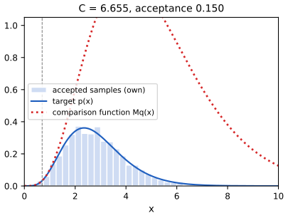
p. 489 To sample \(\Ga(x\given\alpha,\lambda)=\frac1{\Gamma(\alpha)}x^{\alpha-1}\lambda^\alpha e^{-\lambda x}\) (rate parametrisation) with non-integer \(\alpha\), use the proposal \(\Ga(k,\lambda-1)\) with \(k=\lfloor\alpha\rfloor\) (a sum of \(k\) exponential variables, which needs \(\lambda>1\)). The ratio is \[ \frac{p(x)}{q(x)}=\frac{\Gamma(k)\lambda^\alpha}{\Gamma(\alpha)(\lambda-1)^k}\,x^{\alpha-k}e^{-x}, \tag{11.26, 11.27} \] which is maximised at \(x=\alpha-k\), so \(C=\Ga(\alpha-k\given\alpha,\lambda)/\Ga(\alpha-k\given k,\lambda-1)\) (11.28). For \(\alpha=5.7\), \(\lambda=2\) this gives \(C=6.65\), an acceptance rate of \(0.150\). The book's choice of proposal rate \(\lambda-1\) is valid but far from tight: gap 11.5 shows that the best rate is \(k\lambda/\alpha\), for which \(C=1.07\) and the acceptance rate is \(0.935\). The rejection sampling demo lets you vary \(\alpha\), \(\lambda\) and the rule for the proposal rate (preset 2 shows the optimal rate).
Filling the gap 11.5: the gamma envelope, its constant, and the best proposal rate pp. 489, 487–488
Derivation
Sum of exponentials. If \(X_i\sim\Expon(\lambda)\) i.i.d., then \(\E e^{tX_i}=\lambda/(\lambda-t)\) for \(t<\lambda\), so \(Y=X_1+\dots+X_k\) has moment generating function \((\lambda/(\lambda-t))^k\), which is that of \(\Ga(k,\lambda)\); a mgf finite near 0 determines the law. This is the sampler for the proposal.
The ratio. Take a proposal \(\Ga(k,\lambda')\) with rate \(\lambda'\in(0,\lambda)\). Then \[ r(x)=\frac{p(x)}{q(x)}=K\,x^{\alpha-k}e^{-(\lambda-\lambda')x},\qquad K=\frac{\Gamma(k)\lambda^\alpha}{\Gamma(\alpha)\lambda'^{\,k}}. \] We need \(r\) bounded, which requires \(\lambda'<\lambda\) (otherwise, for \(\alpha>k\), \(r(x)\to\infty\) as \(x\to\infty\): the proposal must have the heavier tail), and this is why the book's choice \(\lambda'=\lambda-1\) needs \(\lambda>1\). With \(\alpha-k\in[0,1)\), \(\frac{d}{dx}\log r=\frac{\alpha-k}{x}-(\lambda-\lambda')\) vanishes at \[ x^*=\frac{\alpha-k}{\lambda-\lambda'}, \] and \(\log r\) is concave, so this is the global maximum and \(C=r(x^*)\). For \(\lambda'=\lambda-1\) it is \(x^*=\alpha-k\) and \(C=r(\alpha-k)\), the book's (11.28).
The best rate. At \(x^*\), \[ \ln C(\lambda')=\ln\Gamma(k)+\alpha\ln\lambda-\ln\Gamma(\alpha)-k\ln\lambda'-(\alpha-k)\ln(\lambda-\lambda')+(\alpha-k)\ln(\alpha-k)-(\alpha-k). \] Its derivative \(-k/\lambda'+(\alpha-k)/(\lambda-\lambda')\) vanishes at \(\lambda'=k\lambda/\alpha\), and its second derivative \(k/\lambda'^2+(\alpha-k)/(\lambda-\lambda')^2>0\), so this is the minimiser: the proposal \(\Ga(k,k\lambda/\alpha)\) has the same mean \(\alpha/\lambda\) as the target, and then \(x^*=\alpha/\lambda\). For \(\alpha=5.7,\lambda=2\) the best rate is \(10/5.7=1.754\) and \(C=1.070\); for the book's rate \(1\) it is \(C=6.655\). When \(\alpha\) is an integer, \(\alpha=k\), the best proposal is the target itself and \(C=1\).
11.4.3 Adaptive rejection sampling
pp. 489–490 For a log-concave one-dimensional density, \(h=\log f\) is concave and lies below each of its tangent lines. The minimum of the tangent lines at a set of abscissae \(x_1<\dots<x_k\) is a piecewise-linear upper bound of \(h\), so its exponential is a piecewise-exponential envelope,
\[ q(x)=C_i\lambda_i\exp(-\lambda_i(x-x_{i-1})),\qquad x_{i-1}<x\le x_i, \tag{11.29} \]
(one exponential piece per interval between consecutive breakpoints), which is easy to sample exactly. When a draw is rejected, it is added to the abscissae, the envelope tightens, and the rejection rate falls. This is adaptive rejection sampling (ARS; Gilks and Wild 1992) and works for unnormalised densities. Gap 11.6 proves the envelope property, shows how to sample each piece (including a piece that is unbounded on the left) and shows that adapting the envelope keeps the samples exactly distributed as \(f\). My code is the class ARS.
Filling the gap 11.6: the tangent envelope, sampling it, and why adapting is allowed pp. 489–490
Derivation
Envelope. If \(h\) is concave and differentiable, \(h(x)\le h(x_i)+h'(x_i)(x-x_i)=:\ell_i(x)\) for every \(x\) and every \(i\) (the tangent line lies above a concave function). Hence \(h\le u:=\min_i\ell_i\), and \(f\le e^u\). The function \(u\) is concave and piecewise linear. Consecutive tangents meet at \[ z_i=\frac{h(x_{i+1})-h(x_i)-x_{i+1}h'(x_{i+1})+x_ih'(x_i)}{h'(x_i)-h'(x_{i+1})}\in(x_i,x_{i+1}), \] because \(h'\) is non-increasing; the piece \(j\) of \(u\) is \(\ell_j\) on \([z_{j-1},z_j]\) (with \(z_0=\text{lower end}\), \(z_k=\text{upper end}\) of the support).
Sampling the piece. Write \(s_j=h'(x_j)\), \(a=z_{j-1}\), \(b=z_j\) (if \(s_j=0\) the piece is flat: mass \(e^{\ell_j}(b-a)\) and \(x=a+U(b-a)\); below \(s_j\ne0\)). Its mass is \(m_j=\int_a^be^{\ell_j}=(e^{\ell_j(b)}-e^{\ell_j(a)})/s_j\). Pick piece \(j\) with probability \(m_j/\sum_im_i\), then invert its cdf: the cdf of \(e^{\ell_j}\) on \([a,b]\) is \((e^{\ell_j(x)}-e^{\ell_j(a)})/(s_jm_j)\), so with \(U\sim\Unif(0,1)\) \[ x=a+\frac1{s_j}\ln\big(1+U\,s_jm_je^{-\ell_j(a)}\big). \] If \(b=+\infty\) the slope \(s_j\) must be negative, then \(s_jm_je^{-\ell_j(a)}=-1\) and \(x=a+\ln(1-U)/s_j\), an exponential tail. If \(a=-\infty\) (slope positive) use the mirror form \(x=b+\frac1{s_j}\ln\big(U\,s_jm_je^{-\ell_j(b)}\big)\). So the left-most abscissa needs positive slope and the right-most negative slope when the support is unbounded, otherwise the envelope has infinite mass. For \(f(x)=e^{-x^2/2}\) on \((-\infty,0]\), \(h'(x)=-x>0\) for all \(x<0\), so tangents are always valid on the left and the support ends at \(0\) on the right (Figure 11.5b,c).
Accepting. Given the current envelope \(e^u\), draw \(x\) from \(e^u/\int e^u\) and \(V\sim\Unif(0,1)\), accept if \(V\le f(x)/e^{u(x)}\). This is ordinary rejection sampling with \(C=\int e^u\) (gap 11.4), so an accepted \(x\) has density \(f/\int f\) given the envelope. The envelope depends only on earlier rejected points, and that conditional law does not depend on them, so each accepted draw is distributed as the target given the past, hence the accepted draws are independent with the correct law. Rejected points are used only to refine \(u\) and can never bias the output.
See also: Bayesian and Probabilistic ML, Result 11.8 and Algorithm 11.2 (adaptive rejection sampling).
11.4.4 Rejection sampling in high dimensions
p. 490 The proposal must be close to the target and above it, which is hard in high dimension. Take \(p=\N(0,\sigma_p^2I)\) and \(q=\N(0,\sigma_q^2I)\) in \(D\) dimensions: \(\sigma_q\ge\sigma_p\) is needed for an upper bound, the optimal constant is \(C=(\sigma_q/\sigma_p)^D\), and the acceptance rate \(1/C\) falls exponentially with \(D\). If \(\sigma_q\) is only 1% larger than \(\sigma_p\), then in \(D=1000\) the acceptance rate is \(1.01^{-1000}=1/20{,}959\), about \(1/20{,}000\) as the book says (gap 11.7; Figure 11.9a below).
Filling the gap 11.7: the optimal constant is \((\sigma_q/\sigma_p)^D\) p. 490
Derivation
The ratio of the two normalised densities is \[ \frac{p(x)}{q(x)}=\Big(\frac{\sigma_q}{\sigma_p}\Big)^D\exp\Big(-\frac{\|x\|^2}2\Big(\frac1{\sigma_p^2}-\frac1{\sigma_q^2}\Big)\Big). \] If \(\sigma_q<\sigma_p\) the exponent is positive and grows with \(\|x\|\): the ratio is unbounded, no \(C\) exists. If \(\sigma_q\ge\sigma_p\) the bracket is \(\ge0\), so the ratio is maximal at \(x=0\) and \(C=\sup p/q=(\sigma_q/\sigma_p)^D\). Both densities are normalised, so the acceptance rate is exactly \(1/C=(\sigma_p/\sigma_q)^D\) (gap 11.4). For a ratio \(1+\delta\): \(C=(1+\delta)^D\approx e^{\delta D}\); with \(\delta=0.01\), \(D=1000\) gives \(e^{9.95}\approx20{,}959\). More generally, for any target and proposal that factorise over coordinates, with each coordinate contributing a factor \(c>1\) to the envelope, \(C=c^D\).
See also: Bayesian and Probabilistic ML, Result 11.9 (acceptance falls exponentially with dimension).
11.5 Importance sampling
p. 490 Importance sampling (IS) estimates \(\E[\varphi(x)]=\int\varphi(x)\pi(x)\d x\) (11.30) for a target function \(\varphi\) and a target distribution \(\pi\) (often a posterior \(p(x\given y)\)) by drawing from a proposal \(q\) and weighting: \(\E[\varphi]\approx\sum_nW_n\varphi(x_n)\) (11.31).
11.5.1 Direct importance sampling
p. 491 If the normalised \(\pi\) can be evaluated, write \(\int\varphi\pi=\int\varphi\frac\pi qq\) (11.32); the support of \(q\) must contain that of \(\pi\). With \(x_n\sim q\), \[ \E[\varphi]\approx\frac1{N_s}\sum_n\tilde w_n\varphi(x_n),\qquad\tilde w_n=\frac{\pi(x_n)}{q(x_n)}, \tag{11.33, 11.34} \] which is unbiased (gap 11.8).
11.5.2 Self-normalized importance sampling
pp. 491–492 When only \(\tilde\gamma(x)=Z\pi(x)\) can be evaluated (11.35, 11.36), estimate the normaliser by IS as well and form the ratio (self-normalised IS, SNIS): \[ \E[\varphi]\approx\frac{\frac1{N_s}\sum_n\tilde w_n\varphi(x_n)}{\frac1{N_s}\sum_n\tilde w_n}=\sum_nW_n\varphi(x_n),\quad\tilde w_n=\frac{\tilde\gamma(x_n)}{q(x_n)},\quad W_n=\frac{\tilde w_n}{\sum_{n'}\tilde w_{n'}}, \tag{11.38--11.41} \] equivalently \(\pi(x)\approx\sum_nW_n\delta(x-x_n)\) (11.42), with the by-product \(Z\approx\hat Z=\frac1{N_s}\sum_n\tilde w_n\) (11.43). The estimate is a ratio, hence biased, but the bias vanishes as \(N_s\to\infty\); gap 11.8 derives the bias, the asymptotic variance and the effective sample size.
Filling the gap 11.8: unbiasedness of IS, bias and variance of SNIS, and the effective sample size pp. 491–492
Derivation
Direct IS. If \(\pi(x)>0\Rightarrow q(x)>0\), then \(\E_q[\tilde w\varphi]=\int_{q>0}\frac\pi q\varphi q=\int\varphi\pi\), so the average (11.33) is unbiased, with variance \(\frac1N(\E_q[\tilde w^2\varphi^2]-\mu^2)=\frac1N(\E_\pi[\tilde w\varphi^2]-\mu^2)\), which is finite only if \(\E_\pi[\tilde w\varphi^2]<\infty\). Likewise \(\E_q\tilde w=Z\) in the unnormalised case, so \(\hat Z\) in (11.43) is unbiased for \(Z\).
SNIS is consistent. Let \(A=\frac1N\sum\tilde w_n\varphi(x_n)\), \(B=\frac1N\sum\tilde w_n=\hat Z\). By the strong law \(A\to Z\mu\), \(B\to Z\) almost surely (when \(\E_q[\tilde w|\varphi|]<\infty\)), so \(A/B\to\mu\).
Asymptotic variance. Exactly, \(\frac AB-\mu=\frac{A-\mu B}{B}=\frac{\frac1N\sum_n\tilde w_n(\varphi(x_n)-\mu)}{B}\). The numerator is an average of i.i.d. terms with mean \(\E_q[\tilde w(\varphi-\mu)]=Z\mu-\mu Z=0\) and variance \(\E_q[\tilde w^2(\varphi-\mu)^2]\); the denominator tends to \(Z\). By the central limit theorem and Slutsky, \[ \sqrt N\Big(\frac AB-\mu\Big)\to\N\Big(0,\ \sigma_{\rm SNIS}^2\Big),\qquad \sigma^2_{\rm SNIS}=\frac{\E_q[\tilde w^2(\varphi-\mu)^2]}{Z^2}=\E_\pi\Big[\frac{\pi}{q}(\varphi-\mu)^2\Big]. \] Bias. A second-order expansion of \(A/B\) about \((\E A,\E B)=(Z\mu,Z)\) gives \(\E[A/B]\approx\mu+\frac{\mu\var B-\cov(A,B)}{Z^2}\), and \(\mu\var B-\cov(A,B)=\frac1N\{\mu(\E_q\tilde w^2-Z^2)-(\E_q\tilde w^2\varphi-\mu Z^2)\}=-\frac1N\E_q[\tilde w^2(\varphi-\mu)]\). So \[ \E\Big[\frac AB\Big]-\mu\approx-\frac{\E_q[\tilde w^2(\varphi-\mu)]}{N\,Z^2}=O(1/N), \] which is much smaller than the standard error \(O(1/\sqrt N)\): bias is rarely the issue; variance is.
Effective sample size. The weights should be nearly equal for the estimator to be as good as an i.i.d. average. Since \(\sum_nW_n^2=\frac{\sum\tilde w_n^2}{(\sum\tilde w_n)^2}\approx\frac{\E_q\tilde w^2}{N(\E_q\tilde w)^2}\), \[ \ess=\frac1{\sum_nW_n^2}\approx N\frac{(\E_q\tilde w)^2}{\E_q\tilde w^2}=\frac{N}{1+\var_q(\tilde w)/(\E_q\tilde w)^2}\in[1,N]. \] It equals \(N\) when all weights are equal (\(q=\pi\)) and 1 when one weight dominates. (It is a rule of thumb: the true variance depends on \(\varphi\) as the formula for \(\sigma^2_{\rm SNIS}\) shows.)
See also: All of Statistics, gap 24.8 (self-normalised importance sampling) and gap 24.9 (the effective sample size).
11.5.3 Choosing the proposal
pp. 492 The support of \(q\) must cover that of \(\tilde\gamma\), but a loose cover wastes draws; ideally the proposal also reflects \(\varphi\), as in Figure 11.6 (a schematic of a rare-event target function, not reproduced). One can learn a proposal by maximising the ELBO (Section 10.1.1.2), and importance-weighted autoencoders (Section 10.5.1) can be read as learning a good IS proposal (Domke and Sheldon 2018). Gap 11.9 proves what "ideal" means (the optimal proposal) and works out the Gaussian example of Figure 11.9b, where a proposal with too small a scale has infinite weight variance. The importance sampling demo lets you move and resize a proposal against a bimodal target and watch the weights, the effective sample size and the spread of the SNIS estimates (preset 2: a proposal that misses one mode; preset 3: light tails).
Filling the gap 11.9: the optimal proposal and a worked effective sample size p. 492
Derivation
Optimal proposal. Let \(\varphi\ge0\) and use direct IS. The variance is \(\frac1N(\int\varphi^2\pi^2/q-\mu^2)\). By the Cauchy-Schwarz inequality, \[ \Big(\int\varphi\pi\Big)^2=\Big(\int\frac{\varphi\pi}{\sqrt q}\sqrt q\Big)^2\le\int\frac{\varphi^2\pi^2}{q}\int q=\int\frac{\varphi^2\pi^2}{q}, \] with equality iff \(\varphi\pi/\sqrt q\propto\sqrt q\), i.e. \(q^*\propto\varphi\pi\). Then the variance is \(\frac1N(\mu^2-\mu^2)=0\): every draw gives exactly \(\mu\) (for general sign, \(q^*\propto|\varphi|\pi\) gives variance \(\frac1N((\E_\pi|\varphi|)^2-\mu^2)\)). This \(q^*\) needs \(\mu\) itself to normalise, so it is a guide only: put mass where \(\pi(x)|\varphi(x)|\) is large, which for a rare-event indicator means the rare region (Figure 11.6). For SNIS the same argument applied to \(\sigma^2_{\rm SNIS}=\int\pi^2(\varphi-\mu)^2/q\) gives \(q^*\propto\pi|\varphi-\mu|\) with variance \((\E_\pi|\varphi-\mu|)^2/N\).
Gaussian example (Figure 11.9b). Target \(\pi=\N(0,1)\), proposal \(q=\N(0,s^2)\), weight \(w=\pi/q\). Then \[ \E_q[w^2]=\int\frac{\pi^2}{q}=\frac{s}{\sqrt{2\pi}}\int e^{-x^2(1-1/(2s^2))}\d x=\frac{s}{\sqrt{2-1/s^2}}\quad\text{if }s^2>\tfrac12, \] and \(+\infty\) if \(s^2\le\frac12\) (the integrand does not decay). Since \(\E_qw=1\), \(\ess/N=1/\E_q[w^2]=\sqrt{2-1/s^2}/s\), which equals 1 at \(s=1\), is \(0.46\) at \(s=3\) (a proposal three times too wide wastes more than half the draws), and is 0 for \(s\le1/\sqrt2\): a proposal that is too narrow has infinite weight variance (its tails are too light), the worst case, and the sample estimates of the ESS in the figure then scatter because the weights are dominated by rare, huge values. Lighter tails are more dangerous than heavier tails.
See also: All of Statistics, Theorem 24.5 (the optimal proposal), gap 24.6 (light tails give infinite variance).
11.5.4 Annealed importance sampling (AIS)
pp. 492–494 Annealed importance sampling (Neal 2001) targets a complicated (multimodal, high-dimensional) \(p_0\propto f_0\) by moving from an easy distribution \(p_n\propto f_n\) (for example the prior) through intermediate distributions \[ f_j(x)=f_0(x)^{\beta_j}f_n(x)^{1-\beta_j},\qquad1=\beta_0>\beta_1>\dots>\beta_n=0, \tag{11.44} \] with inverse temperatures \(\beta_j\). Let \(T_j(x,x')=p_j(x'\given x)\) be a Markov kernel that leaves \(p_j\) invariant (built by the methods of Chapter 12, for instance Metropolis-Hastings). The algorithm: draw \(v_n\sim p_n\); for \(j=n,\dots,1\) multiply the weight by \(f_{j-1}(v_j)/f_j(v_j)\) (the ratio of the next distribution to the current one, at the current point) and then move \(v_{j-1}\sim T_{j-1}(v_j,\cdot)\); finally return \(x=v_0\) with the accumulated weight \[ w=\prod_{j=1}^{n}\frac{f_{j-1}(v_j)}{f_j(v_j)}. \tag{11.45, corrected} \] (The printed (11.45) evaluates each ratio after the move, which is not valid for kernels leaving \(p_j\) invariant; see Notes on the book, item 4.) Gap 11.10 shows by an importance-sampling argument on the extended space \(v=(v_0,\dots,v_n)\) that the weighted samples \((v_0,w)\) target \(p_0\) and that the average weight estimates a ratio of normalising constants.
11.5.4.1 Estimating normalizing constants using AIS
p. 494 Since \(Z_0=\int f_0\) and \(Z_n=\int f_n\), \[ \frac{Z_0}{Z_n}=\E_g\Big[\frac{\phi(v)}{g(v)}\Big]\approx\frac1S\sum_{s=1}^Sw_s,\qquad w_s=\frac{\phi(v^s)}{g(v^s)}, \tag{11.51} \] where \(\phi\) is the extended target and \(g\) the extended proposal of the gap box. In the labelling of Section 11.5.4 (\(f_n\) the easy distribution, for example a prior with known \(Z_n\), and \(f_0\) the unnormalised posterior) this estimates the evidence \(Z_0=p(\mathcal D)=Z_n\,\E[w]\); the book's closing sentence swaps the two labels. It is the method of choice for hard partition functions (Gelman and Meng 1998). The book writes the two extended densities as (11.46)–(11.50).
Filling the gap 11.10: annealed importance sampling is unbiased for \(Z_0/Z_n\) and samples \(p_0\) pp. 493–494
Derivation
Setup. \(f_0,\dots,f_n\) are positive unnormalised densities with \(Z_j=\int f_j\) and \(p_j=f_j/Z_j\); \(T_j\) is a kernel leaving \(p_j\) invariant, \(j=0,\dots,n-1\), applied as \(v_{j+1}\mapsto v_j\). The forward law of the run is \[ g(v_0,\dots,v_n)=f_n(v_n)\prod_{j=0}^{n-1}T_j(v_{j+1},v_j)\qquad\Big(\int g=Z_n\Big). \] Reversed kernels. The time reversal of \(T_j\) with respect to \(p_j\) is \(\tilde T_j(v,v')=T_j(v',v)f_j(v')/f_j(v)\) (the book's (11.48)). It is a Markov kernel: \(\int\tilde T_j(v,v')\d v'=\frac1{f_j(v)}\int T_j(v',v)f_j(v')\d v'=\frac{f_j(v)}{f_j(v)}=1\), where the integral equals \(f_j(v)\) by invariance, \(\int T_j(v',v)p_j(v')\d v'=p_j(v)\). Define the extended target \[ \phi(v_0,\dots,v_n)=f_0(v_0)\prod_{j=0}^{n-1}\tilde T_j(v_j,v_{j+1}). \] (The book's (11.46) prints \(\tilde T_2\) where \(\tilde T_1\) is meant.) Integrating out \(v_n\), then \(v_{n-1}\), ..., then \(v_1\), each reversed kernel integrates to 1, so \(\int\phi\,\d v_1\cdots\d v_n=f_0(v_0)\): the \(v_0\)-marginal of \(\phi\) is the target \(f_0\), and \(\int\phi=Z_0\).
The weight. Dividing, \[ \frac{\phi}{g}=\frac{f_0(v_0)}{f_n(v_n)}\prod_{j=0}^{n-1}\frac{f_j(v_{j+1})}{f_j(v_j)}=\prod_{j=1}^{n}\frac{f_{j-1}(v_j)}{f_j(v_j)}, \] since the kernel densities \(T_j\) cancel, and the last equality follows by collecting the factors at each point \(v_j\): \(f_{j-1}(v_j)\) from the numerator product, \(1/f_j(v_j)\) from the denominator product (the extra factors \(f_0(v_0)\) and \(1/f_n(v_n)\) cancel the unmatched ends). This is the weight (11.45, corrected), and it depends only on the visited points.
Unbiased for \(Z_0/Z_n\). With \(v\sim g/Z_n\) (the algorithm's own law), \(\E[\phi/g]=\int\frac\phi g\frac g{Z_n}=\frac{Z_0}{Z_n}\), which is (11.51); the average of \(S\) independent runs is unbiased. In particular, if \(Z_n\) is known (the easy distribution is normalised), \(Z_0=Z_n\E[w]\) is estimated without bias by \(Z_n\) times the average weight.
Samples from \(p_0\). For a test function \(h\) of \(v_0\), \(\E_g[\frac\phi gh(v_0)]=\int\phi\,h(v_0)=Z_0\E_{p_0}h\), so \(\E_g[wh(v_0)]/\E_g[w]=\E_{p_0}h\): \((v_0,w)\) is a self-normalised importance sample for \(p_0\).
Why more steps help. Suppose the kernels were perfect, \(v_j\sim p_j\) independently. With the geometric path \(f_{j-1}/f_j=(f_0/f_n)^{\beta_{j-1}-\beta_j}=\big(f_0/f_n\big)^{\Delta\beta}\) and equal steps \(\Delta\beta=1/n\), \(\log w=\frac1n\sum_{j=1}^nL(v_j)\) with \(L=\log(f_0/f_n)\), so \(\var\log w=\frac1{n^2}\sum_j\var_{p_j}(L)=O(1/n)\). With \(n=1\) the method is plain importance sampling of \(p_0\) from \(p_n\); more temperatures reduce the weight variance, at the price of \(n\) kernel steps per sample. With imperfect kernels the same ordering holds in practice (Figure 11.8).
11.6 Controlling Monte Carlo variance
p. 494 The standard error is \(O(1/\sqrt S)\), so halving it costs four times as many draws. The rest of the chapter shows how to lower the constant instead. The variance reduction demo runs the plain, control-variate, antithetic and randomised quasi-Monte Carlo estimators side by side.
11.6.1 Common random numbers
p. 494 To compare \(\E_{p(z)}[f(\theta,z)]\) with \(\E_{p(z)}[f(\theta',z)]\), evaluate both with the same draws \(z_s\), so that differences are due to \(\theta\) and not to noise; this also turns a stochastic optimisation problem into a deterministic one for fixed \(z_{1:S}\), which allows second-order optimisers (gap 11.11).
Filling the gap 11.11: why common random numbers reduce the variance of a difference p. 494
Derivation
Let \(D_\theta=\frac1S\sum_sf(\theta,z_s)\) and similarly \(D_{\theta'}\). With the same \(z_s\) in both, \(\var(D_\theta-D_{\theta'})=\frac1S\{\var f(\theta,z)+\var f(\theta',z)-2\cov(f(\theta,z),f(\theta',z))\}\); with independent draws the covariance term is absent. So CRN is better exactly when \(\cov(f(\theta,z),f(\theta',z))>0\), which is the typical case when \(f\) is continuous in \(\theta\): then \(\theta'\) near \(\theta\) gives nearly equal values.
Example. \(f(\theta,z)=(\theta-z)^2\) with \(z\sim\N(0,1)\). Then \(f(\theta,z)-f(\theta',z)=\theta^2-\theta'^2-2(\theta-\theta')z\), whose variance per draw is \(4(\theta-\theta')^2\), vanishing as \(\theta'\to\theta\). With independent draws it is \(\var f(\theta,\cdot)+\var f(\theta',\cdot)=(2+4\theta^2)+(2+4\theta'^2)\) per draw. At \(\theta=1\), \(\theta'=1.1\): \(0.04\) against \(12.84\), a factor of 321.
11.6.2 Rao-Blackwellization
pp. 494–495 To estimate \(\E[f(X,Y)]\) from \((X_s,Y_s)\sim p(X,Y)\), the naive estimator is \(\hat f_{\rm MC}=\frac1S\sum_sf(X_s,Y_s)\) (11.52). If \(Y\) can be integrated out analytically, \(f_X(X_s)=\int p(Y\given X_s)f(X_s,Y)\d Y=\E[f(X,Y)\given X=X_s]\) (11.53), the Rao-Blackwellised estimator is \(\hat f_{\rm RB}=\frac1S\sum_sf_X(X_s)\) (11.54). It is unbiased and has smaller variance, by the law of iterated variance (11.55; gap 11.12). Examples in the book are at Sections 6.3.4.2, 13.4 and 12.3.8.
Filling the gap 11.12: the law of total variance and Rao-Blackwellisation p. 495
Derivation
Let \(g(X)=\E[f\given X]\). Unbiased: \(\E g(X)=\E f\) by the tower property. Variance: decompose \(f-\mu=(f-g)+(g-\mu)\). The cross term vanishes: \(\E[(f-g)(g-\mu)]=\E[(g-\mu)\E[f-g\given X]]=0\). Therefore \(\var f=\E[(f-g)^2]+\var g=\E[\var(f\given X)]+\var(\E[f\given X])\), so \[ \var[\E[f(X,Y)\given X]]=\var[f(X,Y)]-\E\big[\var[f(X,Y)\given X]\big]\le\var[f(X,Y)] \tag{11.55} \] (the book writes the second term as \(\E[\var[f]\given X]\); the conditional variance is the object inside the outer expectation). Equality holds iff \(\var[f\given X]=0\) a.s., i.e. \(f\) does not depend on \(Y\) given \(X\). Averaging \(S\) i.i.d. copies divides both variances by \(S\).
Example. \(X\sim\N(0,1)\), \(Y\given X\sim\N(X,1)\), \(f=Y^2\). Marginally \(Y\sim\N(0,2)\), \(\var Y^2=2\cdot2^2=8\). Integrating out \(Y\): \(\E[Y^2\given X]=X^2+1\), variance \(\var(X^2)=2\). And \(\E\var(Y^2\given X)=\E(2+4X^2)=6\); indeed \(8=6+2\). Rao-Blackwellisation cuts the variance by a factor of 4.
See also: this course, gap 6.3 (control variates and Rao-Blackwellisation on a score-function gradient).
11.6.3 Control variates
pp. 495–496 Let \(m(X)\) be an unbiased estimator of \(\mu\) and \(b(X)\) a baseline with known mean \(\E b\). Then \[ m^*(X)=m(X)+c\,\big(b(X)-\E[b(X)]\big) \tag{11.56} \] is also unbiased, with \[ \var[m^*]=\var[m]+c^2\var[b]+2c\cov[m,b],\quad c^*=-\frac{\cov[m,b]}{\var[b]},\quad \var[m^*]=(1-\rho_{m,b}^2)\var[m] \tag{11.57--11.59} \] The estimator exploits the error in estimating the known quantity \(\E b\) to correct the error in estimating the unknown \(\mu\). The coefficient \(c^*\) is estimated from the same samples (gap 11.13).
11.6.3.1 Example
p. 496 Estimate \(\mu=\E[1/(1+X)]=\ln2=0.6931\) for \(X\sim\Unif(0,1)\) with \(S=1500\) draws, using the baseline \(b(X)=1+X\) with \(\E b=3/2\). Exact quantities (gap 11.13): \(\var f=\tfrac12-\ln^22=0.01955\), \(\cov(f,b)=1-\tfrac32\ln2=-0.03972\), \(\var b=\tfrac1{12}\), so \(c^*=0.4766\) (the book's sample estimate is 0.4773), \(\rho^2=0.9686\), and the standard error drops from \(\sqrt{\var f/S}=0.00361\) (book: 0.0037) to \(0.00064\) (book: 0.0007), a factor of 5.6.
Filling the gap 11.13: the optimal coefficient, the variance factor \(1-\rho^2\), and the worked example pp. 495–496
Derivation
Unbiased. \(\E m^*=\E m+c(\E b-\E b)=\mu\) for every \(c\). Variance. Expanding \(\var(m+cb)\) gives (11.57), a convex quadratic in \(c\) (\(\var b>0\)); setting the derivative \(2c\var b+2\cov(m,b)\) to zero gives \(c^*\) (11.58), and substituting, \[ \var m-\frac{\cov(m,b)^2}{\var b}=\var m\Big(1-\frac{\cov(m,b)^2}{\var m\var b}\Big)=(1-\rho_{m,b}^2)\var m. \] So the gain is governed by \(\rho^2\): a perfectly correlated baseline (\(|\rho|=1\)) removes all the variance; an uncorrelated one gives nothing (but \(c^*=0\) means no harm). The sign of \(c\) takes care of positive or negative correlation, and the cost of a baseline is one extra function evaluation.
Estimated \(c\). With \(\hat c\) computed from the same sample, \(m^*(\hat c)\) is not exactly unbiased (it is a nonlinear function of the sample), but \(\sqrt N(m^*(\hat c)-\mu)=\sqrt N(m^*(c^*)-\mu)+(\hat c-c^*)\sqrt N(\bar b-\E b)\), and the last term is a product of a term tending to 0 and one that is \(O_P(1)\), so it tends to 0: the bias is \(O(1/N)\) and the asymptotic variance is \((1-\rho^2)\sigma^2/N\) as for the ideal \(c^*\). The code uses the sample covariance (vr_estimators).
The example. \(f(x)=1/(1+x)\): \(\E f=\ln2\), \(\E f^2=\int_0^1(1+x)^{-2}\d x=\frac12\), so \(\var f=\frac12-\ln^22=0.019547\). \(\E[fb]=\E[1]=1\), so \(\cov(f,b)=1-\tfrac32\ln2=-0.039721\). \(\var b=\var X=\frac1{12}\). Hence \(c^*=-\cov(f,b)/\var b=0.039721\cdot12=0.47665\) (11.58), \(\rho^2=\cov^2/(\var f\var b)=0.96858\), \(\var m^*=0.0314\cdot0.019547=6.14\times10^{-4}\), and for \(S=1500\), \(\operatorname{se}=\sqrt{6.14\times10^{-4}/1500}=6.4\times10^{-4}\). A simulation of 2000 repetitions confirms \(0.0036\) and \(0.0006\).
See also: variance reduction demo, preset 1 (the book's example); preset 2 (a stronger baseline: \(e^x\)).
11.6.4 Antithetic sampling
p. 496 If \(Y_1\), \(Y_2\) are two unbiased draws of \(\theta=\E Y\), then \(\hat\theta=(Y_1+Y_2)/2\) has \(\var\hat\theta=\frac14(\var Y_1+\var Y_2+2\cov(Y_1,Y_2))\) (11.62), smaller than for independent draws when \(\cov(Y_1,Y_2)<0\): so pair each draw with an "opposite" one of the same law. For \(Y\sim\Unif(0,1)\), take \(y'=1-y\).
11.6.4.1 Example
p. 497 For \(\E[1/(1+X)]\) with the same budget of \(2N=1500\) evaluations (\(N=750\) pairs), plain MC has standard error \(0.00361\). Pairing \(f(U)\) with \(f(1-U)\) gives \(\cov(f(U),f(1-U))=\tfrac23\ln2-\ln^22=-0.01835\), so the variance of a pair average is \(\frac12(\var f+\cov)=6.0\times10^{-4}\), and the exact standard error is \(0.00089\) (gap 11.14). The book gives 0.0007 and says it matches the control variate result; the control variate is in fact somewhat better (0.00064), see Notes on the book.
Filling the gap 11.14: when antithetic draws help, and how much pp. 496–497
Derivation
For a pair \((Y_1,Y_2)\) with equal variances \(\sigma^2\), \(\var\frac{Y_1+Y_2}2=\frac{\sigma^2+\cov(Y_1,Y_2)}2=\frac{\sigma^2}2(1+\rho)\). Two independent draws give \(\sigma^2/2\) for the same cost, so the antithetic pair is better iff \(\rho<0\) (equal cost: each pair uses two evaluations).
Monotone functions. If \(f\) is monotone on \([0,1]\) then \(\cov(f(U),f(1-U))\le0\): \(g(u)=f(u)\) and \(h(u)=f(1-u)\) are monotone in opposite senses, so \((g(u)-g(v))(h(u)-h(v))\le0\) for all \(u,v\); taking the expectation over independent \(U,V\) gives \(2\cov(g(U),h(U))\le0\). For \(U\) itself, \(\cov(U,1-U)=-\var U=-\frac1{12}\), correlation \(-1\) (the book writes \(<1\); it should be \(<0\)). Hence for a linear \(f\) the pair average is exactly \(\mu\) with zero variance.
Non-monotone functions. For \(f(x)=(x-\tfrac12)^2\), \(f(1-x)=f(x)\): \(\rho=+1\), the pair average equals either member, and 750 pairs carry only the information of 750 draws: the variance is twice that of 1500 independent draws. Antithetic sampling is not free of risk.
The example. \(\cov(f(U),f(1-U))=\E\big[\frac1{(1+U)(2-U)}\big]-\ln^22\) and \(\frac1{(1+u)(2-u)}=\frac13\big(\frac1{1+u}+\frac1{2-u}\big)\) integrates to \(\frac23\ln2\); so the covariance is \(0.46210-0.48045=-0.018355\), \(\rho=-0.939\), and the pair-average variance is \(\frac12(0.019547-0.018355)=5.96\times10^{-4}\). For \(N=750\) pairs, \(\operatorname{se}=\sqrt{5.96\times10^{-4}/750}=8.9\times10^{-4}\); plain MC with 1500 draws gives \(3.61\times10^{-3}\), a ratio of 4.05.
11.6.5 Quasi-Monte Carlo (QMC)
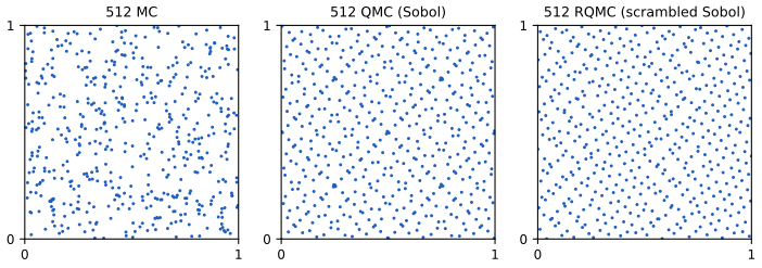
pp. 497–498 Quasi-Monte Carlo replaces random points by a low-discrepancy sequence (Halton, Sobol), which avoids the gaps and clusters of random points (Figure 11.7). For \(f=\int_{[0,1]^D}f(x)\d x\approx\hat f_N=\frac1N\sum_nf(x_n)\) (11.63), MC has error \(O(1/\sqrt N)\) while QMC has error \(O((\log N)^D/N)\), and the book states that for \(N>2^D\) the latter is smaller. QMC gives only a point estimate; randomised QMC (RQMC) repeats the construction \(R\) times with a random shift, \[ y_{i,r}=x_i+u_r\ \ (\mathrm{mod}\ 1),\qquad u_r\sim\Unif(0,1)^D, \tag{11.64} \] so that each \(y_{i,r}\) is uniform and the \(R\) replicates give a standard error (\(R\) is often a power of 2). Orthogonal MC conditions samples to be pairwise orthogonal. Gap 11.15 proves the one-dimensional error bound behind the \(O((\log N)^D/N)\) rate, the unbiasedness of the randomised version, and shows that the "\(N>2^D\)" threshold is too optimistic.
Filling the gap 11.15: the error of QMC, the randomised version, and the "\(N>2^D\)" claim pp. 497–498
Derivation
Discrepancy and the Koksma bound (D = 1). For points \(x_1,\dots,x_N\in[0,1]\) let \(F_N(t)=\frac1N\#\{n:x_n\le t\}\) and the star discrepancy \(D_N^*=\sup_t|F_N(t)-t|\). If \(f\) has bounded variation \(V(f)\) and is continuous, then \[ \hat f_N-\int_0^1f=\int_0^1f\,\d(F_N-t)=-\int_0^1(F_N(t)-t)\,\d f(t), \] by integration by parts (the boundary terms vanish because \(F_N-t\) is 0 at \(t=0\) and at \(t=1\)). Hence \(|\hat f_N-\int f|\le D_N^*V(f)\), Koksma's inequality. For random points \(D_N^*\) is of order \(1/\sqrt N\), but for the van der Corput sequence \(D_N^*\le c\,\log N/N\). In dimension \(D\) the Koksma-Hlawka inequality \(|\hat f_N-\int f|\le D_N^*V_{\rm HK}(f)\) holds with the Hardy-Krause variation, and the best known sequences (Halton, Sobol) have \(D_N^*=O((\log N)^D/N)\); this is the book's rate (see Niederreiter 1992 and Owen 2013 for these results, which I quote, not prove). The bound needs \(f\) of bounded Hardy-Krause variation, a strong smoothness condition.
Randomised QMC is unbiased. For fixed \(x\in[0,1]^D\) and \(u\sim\Unif(0,1)^D\), \(y=x+u\bmod1\) is uniform: translation modulo 1 preserves Lebesgue measure on the torus, so \(\Pr(y\in A)=|A|\) for every box \(A\). Hence \(\E f(y_{i,r})=\int f\) for each \(i\), each replicate \(\hat f_r=\frac1N\sum_if(y_{i,r})\) is unbiased, and replicates with independent \(u_r\) are i.i.d.: \(\bar f=\frac1R\sum_r\hat f_r\) has a standard error \(\hat s/\sqrt R\) computed from the \(R\) values, the missing uncertainty estimate of plain QMC. (Within a replicate the \(N\) points are not independent, so \(N\) points are not used for the variance estimate.) Scrambled Sobol sequences (Owen) are an improved randomisation, with errors that decay faster than \(N^{-1}\) for smooth integrands, as in Figure 11.10c.
The "\(N>2^D\)" threshold. The bound \(g(N)=(\ln N)^D/N\) is increasing on \(1<N<e^D\) (its log-derivative \(D/(N\ln N)-1/N\) is positive iff \(\ln N<D\)), so it is not even a decreasing bound until \(N>e^D\), and it is below the MC rate \(N^{-1/2}\) only when \((\ln N)^D<\sqrt N\). Writing \(t=\ln N\), this is \(D\ln t<t/2\): numerically it first holds permanently for \(N\approx e^{8.6}\approx5.5\times10^3\) at \(D=2\), \(e^{17}\approx2.4\times10^7\) at \(D=3\), \(e^{35.8}\approx3.8\times10^{15}\) at \(D=5\) and \(e^{90}\approx10^{39}\) at \(D=10\), against \(2^D=4,8,32,1024\). So as a statement about the bound, \(N>2^D\) is false for \(D\ge2\). QMC is nevertheless useful at modest \(N\) in moderate dimension because real integrands have low effective dimension and are smooth, and the bound is pessimistic (Figure 11.10c, \(D=5\), where Sobol points beat MC from \(N=64\) on).
Supplement S11 (Monte Carlo inference)
The supplement's Chapter 11 consists of the chapter title page only; there is no additional material for this chapter in the draft.
Demonstrations
Practice problems
The book has no exercises for this chapter. These three short problems are my own.
Practice problem 11.1 (a rare event). Estimate \(p=\Pr(Z>3)\) for \(Z\sim\N(0,1)\) by plain Monte Carlo to within 10% relative error at 95% confidence. How many draws are needed?
Solution
\(f=\ind(Z>3)\) is Bernoulli\((p)\), \(p=0.0013499\), \(\sigma^2=p(1-p)\). The half-width \(1.96\sqrt{p(1-p)/N}\) must be at most \(0.1p\): \(N\ge1.96^2(1-p)/(0.01\,p)=3.8416\cdot0.99865/(0.01\cdot0.0013499)\approx2.84\times10^5\) draws. The relative error is \(\approx1/\sqrt{Np}\), so rare events need \(N\gg1/p\). Importance sampling with \(q=\N(3,1)\) (gap 11.9: put the mass where \(\pi|\varphi|\) is large) needs far fewer: the weights \(\tilde w=e^{-3x+4.5}\) are bounded on the event \(x>3\), by \(e^{-4.5}\), and the variance is that of a single bounded average.
Practice problem 11.2 (inverse cdf). Give a sampler for (a) the density \(p(x)=2x\) on \([0,1]\) and (b) the standard Cauchy density.
Solution
(a) \(F(x)=x^2\) on \([0,1]\), \(F^{-1}(u)=\sqrt u\): draw \(u\sim\Unif(0,1)\) and return \(\sqrt u\). (b) \(F(x)=\frac12+\frac1\pi\arctan x\), so \(F^{-1}(u)=\tan(\pi(u-\tfrac12))\). Both follow from Theorem 11.3.1 (gap 11.2). Check for (a): \(\E x=\int_0^1x\cdot2x\d x=2/3=\E\sqrt U\).
Practice problem 11.3 (a control variate). Estimate \(\E[e^U]=e-1\), \(U\sim\Unif(0,1)\), with the baseline \(b=U\). Compute \(c^*\) and the variance reduction factor.
Solution
\(\var e^U=\frac{e^2-1}2-(e-1)^2=0.24204\). \(\E[Ue^U]=1\), so \(\cov(e^U,U)=1-\frac{e-1}2=0.14086\); \(\var U=\frac1{12}\). Then \(c^*=-\cov/\var b=-1.6903\), \(\rho^2=\cov^2/(\var e^U\cdot\frac1{12})=0.98372\), so the variance is multiplied by \(1-\rho^2=0.016280\), i.e. reduced by a factor of 61.4 (a standard error 7.8 times smaller). The baseline is so well correlated with \(e^U\) because \(e^u\) is nearly linear on \([0,1]\). My code confirms these numbers by simulation.
Notes on the book
Slips and sharpenings found while proving and checking the claims
- Section 11.2.1, the standard error of the \(\pi\) estimate. The book reports \(\hat\pi=3.10\) with standard error \(0.09\) for 5000 samples. The standard error of \(\hat\pi=4\hat p\) is \(\sqrt{\pi(4-\pi)/5000}=0.023\) (gap 11.1); \(0.09\) is the standard error of the area estimate \(\hat I=4\cdot\hat\pi\) for \(r=2\) (\(r^2\cdot0.0232=0.093\)). With the correct standard error, 3.10 is about 1.8 standard errors below \(\pi\), not 0.5.
- Section 11.6.4, the antithetic covariance. "\(\cov[y_i,y_i']<1\)" should read \(<0\); in fact \(\cov(U,1-U)=-1/12\) and the correlation is \(-1\) (gap 11.14).
- Section 11.6.4.1, the antithetic standard error. The exact standard error of the antithetic estimator with 750 pairs is \(0.00089\), not \(0.0007\), and the control variate with 1500 evaluations has \(0.00064\): the two do not "match"; the control variate is about 1.4 times better here. (Plain MC \(0.00361\) matches the book's 0.0037.) Both are confirmed by exact calculation and simulation.
- Section 11.5.4, annealed importance sampling. (a) The text says the kernel \(T_j\) leaves \(p_0\) invariant; it must leave \(p_j\) invariant. (b) In (11.46) \(\tilde T_2\) should be \(\tilde T_1\). (c) As I read (11.45), each ratio \(f_j(v_j)/f_{j+1}(v_j)\) is evaluated at the point obtained after the transition that leaves \(p_j\) invariant. That weight is not valid: for \(n=1\), \(f_0=3\,\N(0,1)\), \(f_1=\N(2,1)\) (so \(Z_0/Z_1=3\)) and \(v_0\sim p_0\) drawn exactly, the mean of \(f_0(v_0)/f_1(v_0)\) is \(3e^4=163.8\), not 3. The weight that equals \(\phi/g\) is \(\prod_{j=1}^nf_{j-1}(v_j)/f_j(v_j)\), evaluated at the point before it is moved (gap 11.10), which is how Neal (2001) states it. (d) The last sentence of 11.5.4.1 calls \(f_0\) the prior and \(f_n\) the posterior, the reverse of the roles in 11.5.4, where \(f_n\) is the easy distribution (the prior) and \(f_0\) the target; with the labels of 11.5.4 the estimator gives \(Z_0=Z_n\E[w]\). I checked these numerically.
- Section 11.6.5, the threshold \(N>2^D\). The bound \((\log N)^D/N\) is smaller than \(1/\sqrt N\) only for much larger \(N\) than \(2^D\) (about \(5\times10^3\), \(2\times10^7\), \(4\times10^{15}\), \(10^{39}\) for \(D=2,3,5,10\)); see gap 11.15. QMC can still beat MC at much smaller \(N\), but not because of this bound.
- Clarification (11.55). The second term is \(\E[\var[f(X,Y)\given X]]\), the expectation of the conditional variance; as printed, "\(\E[\var[f(X,Y)]\given X]\)" is not that object.
References
- Murphy, K. P. (2023). Probabilistic Machine Learning: Advanced Topics. MIT Press, Cambridge, MA. Chapter 11, pp. 483–498. probml.github.io/pml-book/book2.html.
- Domke, J. and Sheldon, D. (2018). Importance weighting and variational inference. Advances in Neural Information Processing Systems, 31.
- Gelman, A. and Meng, X.-L. (1998). Simulating normalizing constants: from importance sampling to bridge sampling to path sampling. Statistical Science, 13(2), 163–185.
- Gilks, W. R. and Wild, P. (1992). Adaptive rejection sampling for Gibbs sampling. Journal of the Royal Statistical Society C, 41(2), 337–348.
- Kroese, D. P., Taimre, T. and Botev, Z. I. (2011). Handbook of Monte Carlo Methods. Wiley.
- Liu, J. S. (2001). Monte Carlo Strategies in Scientific Computing. Springer.
- Neal, R. M. (2001). Annealed importance sampling. Statistics and Computing, 11(2), 125–139.
- Niederreiter, H. (1992). Random Number Generation and Quasi-Monte Carlo Methods. SIAM.
- Owen, A. B. (2013). Monte Carlo Theory, Methods and Examples. Online book.
- Owen, A. B. and Rudolf, D. (2021). A strong law of large numbers for scrambled net integration. SIAM Review, 63(2), 360–372.
- Robert, C. P. and Casella, G. (2004). Monte Carlo Statistical Methods, 2nd edition. Springer.
The numerical statements in the text (the standard error of the \(\pi\) estimate and the confidence-interval coverage, the inverse-cdf, polar Box-Muller and gamma samplers against their target laws, the gamma envelope constant and its optimal proposal rate, the adaptive rejection sampler, the exponential decay of the acceptance rate, the unbiasedness, bias and variance of importance sampling and the effective sample size, the unbiasedness of annealed importance sampling and the failure of the printed weights, the exact standard errors of the control-variate, antithetic and quasi-Monte Carlo estimators, and the practice problems) were confirmed numerically.