Predictive models: an overview
A predictive model is a conditional distribution \(p(y\given x)\) learned from labelled examples. This chapter, the opening of Part III, maps the family of such models (linear, neural, non-parametric, developed in Chapters 15 to 19), shows how fitting by maximum likelihood, empirical risk minimisation, MAP, Bayes and variational inference all descend from one variational objective, and then concentrates on how to evaluate a prediction: proper scoring rules, calibration and its repair by temperature scaling and binning, the difference between aleatoric and epistemic uncertainty in joint predictions, and conformal prediction, which gives finite-sample coverage guarantees from exchangeability alone. The notes prove each result the book states without proof and reproduce the computed figures with my own code.
Ch. 1 Introduction Ch. 2 Probability Ch. 3 Statistics Ch. 4 Graphical models Ch. 5 Information theory Ch. 6 Optimisation Ch. 7 Inference algorithms Ch. 8 Gaussian filtering Ch. 9 Message passing Ch. 10 Variational inference Ch. 11 Monte Carlo Ch. 12 MCMC Ch. 13 Sequential Monte Carlo Ch. 14 Predictive models Ch. 15 GLMs Ch. 16 Deep networks Ch. 17 Bayesian neural networks Ch. 18 Gaussian processes Ch. 19 Beyond iid Ch. 20 Generative models Ch. 21 VAEs Ch. 22 Autoregressive models Ch. 23 Normalizing flows Ch. 24 Energy-based models Ch. 25 Diffusion models Ch. 26 GANs Ch. 27 Discovery methods Ch. 28 Latent factor models Ch. 29 State-space models Ch. 30 Graph learning Ch. 31 Nonparametric Bayes Ch. 32 Representation learning Ch. 33 Interpretability Ch. 34 Decision making Ch. 35 Reinforcement learning Ch. 36 Causality
How to read these notes
They follow the book. Sections carry the book's numbers and equations keep theirs where the draft numbers them (e.g. (14.29), (14.49)). This chapter opens Part III, on models for prediction \(p(y\given x)\). It names the families of model (developed in Chapters 15 to 19), the ways of fitting them (maximum likelihood, MAP, empirical risk minimisation, Bayes, variational inference) and, most of the chapter, how to evaluate a predictive model: proper scoring rules, calibration and conformal prediction.
Filling the gaps. Wherever the book states a result without proof, an orange Filling the gap box gives the full argument. Proofs start hidden.
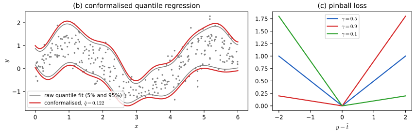
Figures. Figure 14.1 in the book uses a ResNet on CIFAR-100, which is too large to train here; it is replaced by synthetic over-confident scores that show the same effect, and the caption says so. Figures 14.2, 14.3 and 14.5b,c are computed from simulated data, with my own implementations of temperature scaling, Platt scaling, histogram binning, pool-adjacent-violators isotonic regression, the scaling-binning calibrator, quantile regression and split conformal prediction. Figures 14.4 and 14.5a show prediction sets for ImageNet images from a large pretrained network and are not reproduced. One further figure (own) shows how the coverage of conformal prediction is distributed.
Main reference
K. P. Murphy, Probabilistic Machine Learning: Advanced Topics, MIT Press (2023; December 2025 draft), Chapter 14, pages 575–590 (book page: probml.github.io/pml-book/book2.html). The explanations, derivations, figures and code are my own.
Companion courses
- Probabilistic Machine Learning: An Introduction: 5.1.6 probabilistic prediction problems (proper scoring rules, calibration), 5.4 empirical risk minimisation, 4.2 maximum likelihood and 4.5 regularisation (MAP), Chapter 10 logistic regression (the model that Platt scaling reuses).
- Bayesian and Probabilistic Machine Learning: 4.3 probabilistic discriminative models, 6.4 Gaussian processes (the non-parametric predictive model).
- All of Statistics: 22.8 assessing error rates, Chapter 13 (prediction intervals).
- Introduction to Statistical Learning: Chapter 5 resampling (cross-validation, the alternative to a held-out calibration set).
What this chapter adds: the Gibbs posterior that unifies ERM, Bayes and variational inference, calibration measures and recalibration methods, the evaluation of joint (not just marginal) predictions, and distribution-free conformal prediction with its finite-sample guarantee.
The chapter at a glance
- 14.1 Parametric and non-parametric predictive models; MLE, ERM and MAP (gap 14.1); Bayes, VI and generalised Bayes as the minimisers of one variational objective (gap 14.2).
- 14.2 Proper scoring rules: log score and Brier score (gap 14.3); calibration, ECE, temperature and Platt scaling, histogram binning and isotonic regression (gap 14.4); joint predictions and the epistemic-aleatoric distinction (gap 14.5).
- 14.3 Conformal prediction: a finite-sample coverage guarantee from exchangeability alone (gap 14.6), applied to classification, quantile regression and Bayesian predictive densities (gap 14.7).
Notation. Data \(\mathcal D=\{(x_n,y_n)\}_{n=1}^N\) with \(x_n\in\mathcal X\), \(y_n\in\mathcal Y\); \(f(x)_c=p(y=c\given x)\) is a classifier's predicted probability; \(\hat p_n=\max_cf(x_n)_c\) its confidence; \(\alpha\in(0,1)\) a miscoverage level.
14.1 Introduction
p. 575 Most of machine learning learns a function from inputs \(x\in\mathcal X\subseteq\mathbb R^D\) to outputs \(y\in\mathcal Y\subseteq\mathbb R^C\) from a labelled training set, and models the uncertainty about the right output by a conditional distribution \(p(y\given f(x))\). For discrete \(y\) this is a discriminative model (a classifier); for real \(y\), a regression model; the book uses the generic name predictive model. It is a special case of a conditional generative model (Chapter 20), distinguished by a low-dimensional output with one best answer.
14.1.1 Types of model
pp. 575–576 Parametric models have a number of parameters that does not grow with the data, and are fast to use but less flexible; non-parametric models store the training examples and predict from a similarity-weighted combination of their labels, \(\hat y=\sum_ns_ny_n\) with \(s_n=K(x,x_n)\ge0\): more flexible, slower. Gaussian processes (Chapter 18) are the leading example; nearest-neighbour models are in the first volume (Chapter 16). A parametric model has the form \(p(y\given f(x;\theta))\) where \(f\) outputs the parameters (a mean, or logits) of the output distribution. If \(f\) is linear in \(\theta\), \(f=\theta^\T\phi(x)\) for a fixed feature map, it is a generalised linear model (Chapter 15); if \(f\) is nonlinear and differentiable it is typically a neural network (Chapter 16, with Bayesian versions in Chapter 17); trees and forests are in the first volume. Chapter 19 relaxes the i.i.d. assumption (distribution shift, domain adaptation).
14.1.2 Model fitting using ERM, MLE, and MAP
p. 576 Maximum likelihood minimises the scaled negative log-likelihood \[ \hat\theta_{\rm mle}=\argmin_\theta\ \frac1N\sum_{n=1}^N\ell_n(\theta),\qquad\ell_n(\theta)=-\log p(y_n\given x_n,\theta), \] for i.i.d. data. Replacing the log loss by a general loss \(\ell\) gives empirical risk minimisation, \(r(\theta)=\frac1N\sum_n\ell_n(\theta)\), and adding a penalty \(\lambda C(\theta)\) (a complexity measure) guards against overfitting. With the log loss, \(C(\theta)=-\log\pi_0(\theta)\) for a prior \(\pi_0\) and a suitable \(\lambda\), this is MAP estimation (gap 14.1). All of these are optimisation problems, solved by the methods of Chapter 6.
Filling the gap 14.1: MAP is penalised ERM with the log loss p. 576
Derivation
For i.i.d. data and prior \(\pi_0\), \(\log p(\theta\given\mathcal D)=\sum_n\log p(y_n\given x_n,\theta)+\log\pi_0(\theta)-\log p(\mathcal D)\), and the last term does not depend on \(\theta\). Therefore \[ \hat\theta_{\rm map}=\argmax_\theta\Big[\sum_n\log p(y_n\given x_n,\theta)+\log\pi_0(\theta)\Big]=\argmin_\theta\Big[\sum_n\ell_n(\theta)-\log\pi_0(\theta)\Big]. \] Dividing the objective by \(N>0\) does not change the minimiser, so \(\hat\theta_{\rm map}=\argmin_\theta\{r(\theta)+\frac1N(-\log\pi_0(\theta))\}\), which is the regularised empirical risk with \(C=-\log\pi_0\) and \(\lambda=1/N\). The factor \(1/N\) records that the prior matters less as the data grow. Example: \(\pi_0=\mathcal N(0,\tau^2I)\) gives \(C(\theta)=\|\theta\|^2/(2\tau^2)\), i.e. ridge or weight decay.
See also: Introduction volume, 4.5 regularisation; 4.3 empirical risk minimisation.
14.1.3 Model fitting using Bayes, VI, and generalized Bayes
p. 577 Instead of a point estimate, estimate a distribution \(q(\theta)\) over parameters. Minimising the expected empirical risk \(\E_q[r(\theta)]\) alone collapses \(q\) to a delta at the ERM solution, so it does not prevent overfitting; the fix is to keep \(q\) close to the prior \(\pi_0\) in KL divergence: \[ q^*=\argmin_{q\in\mathcal P(\Theta)}\ \E_{q(\theta)}[r(\theta)]+\frac1\lambda\,\KL(q\,\|\,\pi_0),\qquad q^*(\theta)=\frac{\pi_0(\theta)e^{-\lambda r(\theta)}}{Z_\lambda}. \tag{Gibbs posterior} \] The minimiser is the Gibbs posterior used in PAC-Bayes theory (gap 14.2). Taking the log loss and \(\lambda=N\) gives exactly the Bayes posterior \(\propto\pi_0(\theta)\prod_np(y_n\given x_n,\theta)\). Restricting the search to a family \(\mathcal Q(\Theta)\subset\mathcal P(\Theta)\) gives variational inference (Chapter 10): minimise \(\E_q[-\log p(\mathcal D\given\theta)]+\KL(q\|\pi_0)\), the negative ELBO. Replacing the log loss by a general risk and the KL by a general divergence \(D(q\|\pi_0)\) weighted by \(\lambda\) gives generalised Bayesian inference, for models that are known to be misspecified.
Filling the gap 14.2: the Gibbs posterior solves the variational problem; Bayes and VI as special cases p. 577
Derivation
Let \(\pi_0\) have a density and let \(Z_\lambda=\int\pi_0(\theta)e^{-\lambda r(\theta)}\d\theta<\infty\); define \(q^*=\pi_0e^{-\lambda r}/Z_\lambda\). For any \(q\ll\pi_0\) with \(\E_q[r]<\infty\), \(\log\frac{q}{\pi_0}=\log\frac{q}{q^*}+\log\frac{q^*}{\pi_0}=\log\frac q{q^*}-\lambda r-\log Z_\lambda\). Taking the expectation under \(q\), \[ \KL(q\|\pi_0)=\KL(q\|q^*)-\lambda\E_q[r]-\log Z_\lambda\ \Longrightarrow\ \E_q[r]+\frac1\lambda\KL(q\|\pi_0)=\frac1\lambda\KL(q\|q^*)-\frac1\lambda\log Z_\lambda. \] The right side is minimised exactly at \(q=q^*\) (where \(\KL(q\|q^*)=0\), by Gibbs' inequality) with optimal value \(-\frac1\lambda\log Z_\lambda\); the minimiser is unique. This identity also shows what the KL regulariser does: the objective for a general \(q\) is the KL to the Gibbs posterior plus a constant, so restricting \(q\) to a family \(\mathcal Q\) (VI) is the same as finding the member of \(\mathcal Q\) closest in \(\KL(q\|q^*)\). Bayes: with \(r(\theta)=-\frac1N\sum_n\log p(y_n\given x_n,\theta)\) and \(\lambda=N\), \(e^{-\lambda r}=\prod_np(y_n\given x_n,\theta)\), so \(q^*\propto\pi_0\prod_np(\cdot)\), the Bayes posterior, and \(-\frac1\lambda\log Z_\lambda=-\frac1N\log p(\mathcal D)\): the optimal value is the negative per-example log evidence, so the ELBO is \(-N\) times the objective. VI: the objective with \(\lambda=N\) is \(\frac1N(\E_q[-\log p(\mathcal D\given\theta)]+\KL(q\|\pi_0))=-\frac1N\ELBO\). Numerically (a grid over \(\theta\) for the example of Chapter 7, with 10 heads and 1 tail) the Gibbs posterior with \(\lambda=N\) reproduces Beta(11,2), and random perturbations of it always increase the objective.
14.2 Evaluating predictive models
14.2.1 Proper scoring rules
p. 578 A scoring rule \(S(p_\theta,(y,x))\) assigns a number to the predictive distribution \(p_\theta(y\given x)\) when the outcome is \(y\); larger is better. Averaged over the true distribution \(p^*\), the expected score is \(S(p_\theta,p^*)=\E_{p^*(x)p^*(y\given x)}[S(p_\theta,(y,x))]\). The rule is proper if \(S(p_\theta,p^*)\le S(p^*,p^*)\) for every \(p_\theta\), with equality iff \(p_\theta=p^*\) (strictly proper): reporting the truth is the best policy, so maximising the score forces the model towards the true probabilities. The log score \(\log p_\theta(y\given x)\) (whose negative is the NLL or log loss) is proper by Gibbs' inequality; the Brier score \(-\sum_c(p_c-\ind(y=c))^2\), a negative squared error between the predicted probability vector and the one-hot label, is also proper and is less sensitive to rare events, whereas the log loss can over-emphasise tail probabilities (gap 14.3). For a Bayesian model replace \(p_\theta\) by the posterior predictive \(\int p_\theta\,p(\theta\given\mathcal D)\d\theta\).
Filling the gap 14.3: the log score and the Brier score are strictly proper p. 578
Derivation
Work pointwise in \(x\) with a categorical truth \(p^*=(p^*_1,\dots,p^*_C)\) and a forecast \(p\) in the simplex (the general case integrates over \(x\)). Log score. \(\E_{y\sim p^*}[\log p_y]=\sum_cp^*_c\log p_c\), so \[ \sum_cp_c^*\log p^*_c-\sum_cp^*_c\log p_c=\KL(p^*\|p)\ge0, \] with equality iff \(p=p^*\) (Gibbs' inequality, from \(\log t\le t-1\): \(-\KL(p^*\|p)=\sum_cp^*_c\log\frac{p_c}{p^*_c}\le\sum_cp^*_c(\frac{p_c}{p^*_c}-1)=0\), with equality iff \(p_c/p^*_c=1\) wherever \(p^*_c>0\)). Hence \(S(p,p^*)\le S(p^*,p^*)\) with the log score; the gap is the KL divergence. Brier. With \(Y\) one-hot, \(\E\|p-Y\|^2=\|p\|^2-2p^\T p^*+1\) (since \(\E Y=p^*\) and \(\|Y\|^2=1\)). Add and subtract \(\|p^*\|^2\): \(\E\|p-Y\|^2=\|p-p^*\|^2+(1-\|p^*\|^2)\). The second term does not depend on the forecast, so the expected (negative) Brier score is \(-\|p-p^*\|^2-(1-\|p^*\|^2)\), maximised uniquely at \(p=p^*\), where it equals \(-(1-\|p^*\|^2)=-\sum_cp^*_c(1-p^*_c)\). This also shows the Brier score is bounded (between \(-2\) and \(0\)) while the log score is unbounded below, which is the sense in which the log loss emphasises tail probabilities. Both statements were confirmed numerically on random forecasts for a three-class truth.
14.2.2 Calibration
pp. 578–582 A classifier is calibrated if its predicted probabilities match empirical frequencies: of the cases it labels with confidence 0.9, about 90% should be right. Optimising a proper score should in principle give calibration, but unbalanced data, overfitting and distribution shift break it.
14.2.2.1 Expected calibration error
Split the confidences \(\hat p_n=\max_cf(x_n)_c\) into \(B\) bins \(I_b=(\frac{b-1}B,\frac bB]\) with index sets \(B_b\). The bin accuracy is \(\operatorname{acc}(B_b)=\frac1{|B_b|}\sum_{n\in B_b}\ind(\hat y_n=y_n)\) and the average confidence \(\operatorname{conf}(B_b)=\frac1{|B_b|}\sum_{n\in B_b}\hat p_n\); plotting accuracy against confidence is a reliability diagram, and the gap is summarised by the expected calibration error \[ \operatorname{ECE}=\sum_{b=1}^B\frac{|B_b|}N\,\big|\operatorname{acc}(B_b)-\operatorname{conf}(B_b)\big|. \] It looks only at the top label; the marginal or static calibration error extends it to every class with importance weights \(w_c\) (with \(w_c=1/C\) when all classes matter equally), and good ECE can coexist with poor static calibration.
14.2.2.2–14.2.2.5 Improving calibration: Platt scaling, binning, temperature scaling
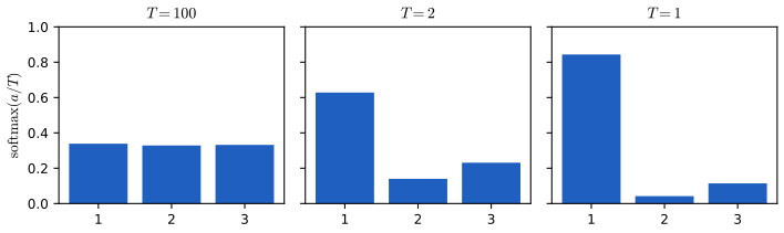
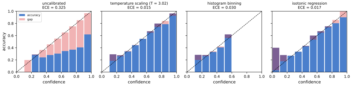
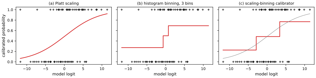
Recalibration maps the model's output to a better probability using a held-out validation set. Platt scaling (binary) replaces a logit \(z\) by \(q=\sigma(az+b)\), with \(a,b\) fitted by maximum likelihood on the validation set, which is a two-parameter logistic regression (the model of first-volume Chapter 10); matrix scaling uses \(q=\softmax(\bm Wz+\bm b)\) and, with \(K^2\) parameters, overfits unless \(\bm W\) is restricted. Histogram binning replaces each probability by the average label in its bin; isotonic regression fits a non-decreasing piecewise constant map; the scaling-binning calibrator first applies Platt scaling and then bins, averaging the scaled probabilities instead of the labels in each bin, which lowers variance. For several classes, the one-vs-rest versions need \(K\) separate maps and the outputs are not normalised. The simplest and in practice the most effective multiclass method is temperature scaling, \(q=\softmax(z/T)\) with \(T>0\) fitted on the validation set (Figure 14.3). It has one parameter, so it cannot overfit, and it never changes which class is most probable, so accuracy is unchanged (gap 14.4).
Filling the gap 14.4: properties of temperature scaling, and convexity of the fitting problem pp. 580–581
Derivation
Accuracy is preserved. Let \(z\in\mathbb R^K\) be the logits. For \(T>0\), \(q_c=e^{z_c/T}/\sum_je^{z_j/T}\), and \(t\mapsto e^{t/T}\) is strictly increasing, so \(q_c>q_{c'}\iff z_c>z_{c'}\): the order of the classes, and thus the arg max, is the same for every \(T>0\). The same is true of Platt scaling for \(a>0\) in the binary case and of any strictly increasing recalibration map.
Limits. As \(T\to\infty\), \(z_c/T\to0\) and \(q\to(1/K,\dots,1/K)\), the uniform distribution; as \(T\to0^+\), the largest logit dominates and \(q\to\) the one-hot vector on \(\argmax z\) (if the maximum is unique). \(T\) moves the model along a one-parameter family from maximum uncertainty to maximum confidence, with \(T=1\) the original. Entropy increases with \(T\) (Figure 14.3).
Unique fit. Put \(\beta=1/T>0\). The validation NLL is \(\operatorname{NLL}(\beta)=\sum_n\big[\lse(\beta z_n)-\beta z_{n,y_n}\big]\), where \(\lse(u)=\log\sum_je^{u_j}\). The log-sum-exp is convex and \(\beta\mapsto\beta z_n\) is linear, so the first term is convex in \(\beta\); the second is linear; hence the NLL is convex in \(\beta\) and any local minimiser (found by a one-dimensional search) is global. Its derivative is \(\sum_n[\,z_n^\T q(\beta z_n)-z_{n,y_n}]\), which vanishes when the model's average expected logit equals the average observed-class logit; the second derivative is \(\sum_n\operatorname{var}_{c\sim q}(z_{n,c})\ge0\). In the experiment of Figure 14.1 the synthetic scores are the true logits times 3 plus a little noise; the fitted temperature is \(T=3.02\), recovering the inflation factor, and it reduces the ECE from 0.325 to 0.015. The minimiser of the NLL need not minimise the ECE in general (a mis-specified model can have a calibrated average confidence and a poorly calibrated bin structure), which is why ECE is reported separately.
14.2.2.6 Label smoothing
pp. 581–582 Instead of the one-hot target \(y=(0,1,0)\), train on a softened target such as \((0.1,0.8,0.1)\), which spreads some mass over the other classes. It prevents the logits from growing without bound (a one-hot target is only approached as the logit gap goes to infinity) and usually improves calibration.
14.2.2.7 Bayesian methods
p. 582 A Bayesian predictive that integrates over parameter uncertainty is usually better calibrated than a plug-in, though even Bayesian models become miscalibrated under distribution shift (Chapter 19, Chapter 17).
14.2.3 Beyond evaluating marginal probabilities
pp. 582–584 Calibration concerns the marginal \(p(y\given x)\). In online learning and sequential decision making this can hide important differences. Two agents see coin tosses \(Y_t\sim\operatorname{Ber}(\theta)\). Agent 1 believes \(\theta=2/3\); agent 2 believes \(\theta\in\{0,1\}\) with probabilities \(1/3\) and \(2/3\). Both predict \(P(Y_{\rm next}=1)=2/3\), but over three tosses agent 1 gives \((2/3)^3=8/27\approx0.30\) to all heads while agent 2 gives \(2/3\): the first agent's uncertainty is aleatoric (irreducible noise), the second's is epistemic (ignorance of \(\theta\), reducible by data). A casino bettor facing agent 2's beliefs would be wise to explore first. This motivates evaluating the joint predictive distribution over \(\tau\) future outcomes \(y=Y_{T+1:T+\tau}\) at \(\tau\) inputs \(x\), given the past \(\mathcal D_T\). With true environment \(E\) (unknown), the Bayes-optimal predictive is \(P(y\given x,\mathcal D_T)=\int P(y\given x,E)P(E\given\mathcal D_T)\d E\), and an agent \(Q\) is scored by an expected KL divergence from the truth, averaged over environments and data, \[ d^{\rm KL}_{E,Q}=\E_{P(x,\mathcal D_T,E)}\big[\KL\big(P(y\given x,E)\,\|\,Q(y\given x,\mathcal D_T)\big)\big]. \] It cannot be computed without knowing \(P(y\given x,E)\), but ranking agents by it is the same as ranking by the cross-entropy, i.e. the NLL of \(Q\) on samples from the environment (the difference is a constant in the agent). In practice one samples \(J\) environments, draws a training set and \(N\) test sequences from each, and averages the log-probabilities: this is the "neural testbed" idea. Good joint accuracy (\(\tau>1\)) correlates with good performance on bandits and active learning (Chapter 34).
14.2.3.1 Proof of the decomposition (14.29)
Filling the gap 14.5: the KL to the environment equals the KL to the Bayes predictive plus a mutual information p. 583, (14.29), (14.40)
Derivation
Condition on \((x,\mathcal D_T)\) and write \(P(y\given x,E)\) for the true predictive. The key fact is that the past data carry no information about the future beyond the environment, \(P(y\given x,E,\mathcal D_T)=P(y\given x,E)\) (given \(E\), the data are i.i.d. draws). Let \(P_B(y)=P(y\given x,\mathcal D_T)\) be the Bayes predictive. Then, with the expectation over \(P(E,y\given x,\mathcal D_T)\), \[ \E\Big[\log\frac{P(y\given x,E)}{Q(y\given x,\mathcal D_T)}\Big]=\E\Big[\log\frac{P_B(y)}{Q(y\given x,\mathcal D_T)}\Big]+\E\Big[\log\frac{P(y\given x,E)}{P_B(y)}\Big]. \] The first expectation depends on \(E\) only through \(y\), whose marginal given \((x,\mathcal D_T)\) is \(P_B\), so it equals \(\KL(P_B\|Q)\), the distance of the agent from the Bayes-optimal one. The second equals \(\E\big[\log\frac{P(E,y\given x,\mathcal D_T)}{P(E\given x,\mathcal D_T)P(y\given x,\mathcal D_T)}\big]\) (using \(P(y\given x,E,\mathcal D_T)=P(y\given x,E)\)), which is the conditional mutual information \(I(y;E\given x,\mathcal D_T)\ge0\). Averaging over \((x,\mathcal D_T)\), \[ d^{\rm KL}_{E,Q}=\underbrace{\E\,\KL(P_B\|Q)}_{\text{the agent's own shortfall}}+\underbrace{I(y;E\given x,\mathcal D_T)}_{\text{epistemic uncertainty, independent of the agent}}. \] So ranking agents by \(d^{\rm KL}_{E,Q}\) is the same as ranking by their KL to the Bayes predictive, which is what a good agent should minimise, and no agent can go below the mutual information: that is the irreducible price of not knowing the environment. A small enumeration (two environments with \(\theta=0.2\) or \(0.9\), one observed toss, \(\tau=2\) future tosses, and a Beta(1,1) agent) reproduces the identity exactly.
14.3 Conformal prediction
pp. 584–589 Conformal prediction turns any predictor into a set (or interval) with guaranteed frequentist coverage, assuming only that the data are exchangeable. Start from a heuristic uncertainty (the softmax score, a predicted variance) and define a conformal score \(s(x,y)\in\mathbb R\) that is large when \(y\) conforms badly to \(x\). Compute the scores \(s_i=s(x_i,y_i)\) on a calibration set of \(n\) labelled examples not used for training (split conformal prediction), take the quantile \[ \hat q=\text{the }\lceil(n+1)(1-\alpha)\rceil\text{-th smallest of }s_1,\dots,s_n\ \ (\hat q=\infty\text{ if }\lceil(n+1)(1-\alpha)\rceil>n), \] and output \(\mathcal T(x_{n+1})=\{y:s(x_{n+1},y)\le\hat q\}\). The remarkable result is \[ 1-\alpha\ \le\ P^*\big(y_{n+1}\in\mathcal T(x_{n+1})\big)\ \le\ 1-\alpha+\frac1{n+1}, \] for every \(n\ge1\), every \(\alpha\in[0,1]\) and every data distribution (upper bound when the scores are almost surely distinct); the probability is over both the calibration set and the new point (gap 14.6). It is not a free lunch: the trivial set of all labels also covers, so the goal is the smallest sets meeting the guarantee, which depends on the score. The guarantee is marginal (an average over inputs), not conditional on a particular \(x\), and frequentist: it is not a per-instance Bayesian statement. Exchangeability excludes serially correlated time series and distribution shift (extensions exist).
Filling the gap 14.6: the finite-sample coverage guarantee, and the exact law of the coverage pp. 584–585, the coverage bound
Derivation
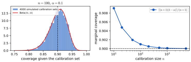
Let \(S_1,\dots,S_n,S_{n+1}\) be the scores of the \(n\) calibration points and the test point; since the pairs \((x_i,y_i)\) are exchangeable and the score function is fixed in advance, \(S_1,\dots,S_{n+1}\) are exchangeable. Assume first that they are almost surely distinct. By exchangeability the rank of \(S_{n+1}\) among the \(n+1\) values is uniform on \(\{1,\dots,n+1\}\), each with probability \(1/(n+1)\). Let \(k=\lceil(n+1)(1-\alpha)\rceil\) and \(\hat q=S_{(k)}\), the \(k\)-th smallest of the first \(n\) scores (if \(k>n\), \(\hat q=\infty\) and coverage is 1). The event \(\{y_{n+1}\in\mathcal T(x_{n+1})\}=\{S_{n+1}\le\hat q\}\) happens exactly when \(S_{n+1}\) has rank at most \(k\) among the \(n+1\) scores (for \(S_{n+1}\le S_{(k)}\), at most \(k-1\) of the calibration scores are below it, so its overall rank is \(\le k\), and conversely). Hence \[ P(S_{n+1}\le\hat q)=\frac{k}{n+1}=\frac{\lceil(n+1)(1-\alpha)\rceil}{n+1}. \] Because \(\lceil u\rceil\ge u\) and \(\lceil u\rceil<u+1\), we get \(1-\alpha\le k/(n+1)<1-\alpha+1/(n+1)\). When ties occur, the lower bound still holds (a tie can only enlarge the set \(\{S_{n+1}\le\hat q\}\), by breaking ties at random one reduces to the distinct case); the upper bound needs distinct scores (Lei et al. 2018). The marginal coverage for \(n=19\), \(\alpha=0.1\) is \(18/20=0.9\) exactly (simulation: 0.9005).
Conditional on the calibration set. With i.i.d. continuous scores let \(F\) be their cdf; \(F(S_i)\) are i.i.d. \(U(0,1)\), so the actual coverage given the calibration set, \(F(\hat q)\), is the \(k\)-th order statistic of \(n\) uniforms, distributed as \(\operatorname{Beta}(k,n+1-k)\). For \(n=100\), \(\alpha=0.1\): \(k=91\), \(\operatorname{Beta}(91,10)\) with mean \(91/101=0.901\) and standard deviation \(0.030\): a particular calibration set can leave coverage a few percent below 90% even though the average is 90.1%. The own figure below shows the simulated and exact distributions agree.
14.3.1 Conformalizing classification
p. 586 The simplest score for a classifier \(f\) is \(s(x,y)=1-f(x)_y\), giving prediction sets \(\mathcal T(x)=\{y:f(x)_y\ge1-\hat q\}\): all labels above a probability threshold. These sets have the smallest average size (Sadinle et al. 2019) but are too big on easy inputs and too small on hard ones. Adaptive prediction sets (Romano et al. 2020) sort the probabilities, \(f(x)_{\pi_1}\ge f(x)_{\pi_2}\ge\cdots\), and use as score the cumulative mass \(s(x,y)=\sum_{c=1}^kf(x)_{\pi_c}\) up to and including the true label \(y=\pi_k\); the set contains the labels, in decreasing order of probability, until the mass reaches \(\hat q\). It uses all the softmax scores, which improves adaptivity (Figures 14.4 and 14.5a in the book, ImageNet examples, are not reproduced).
14.3.2 Conformalizing regression
pp. 586–587 For \(y\in\mathbb R\) one outputs an interval. 14.3.2.1 Conformalized quantile regression (CQR). Fit the \(\gamma\)-quantile \(t_\gamma(x)\) of \(p(y\given x)\) by minimising the pinball (quantile) loss \(\rho_\gamma(y-\hat t)=\max\{\gamma(y-\hat t),(\gamma-1)(y-\hat t)\}\) (Figure 14.5c); the lower and upper fits \(\hat t_{\alpha/2}\) and \(\hat t_{1-\alpha/2}\) give an approximate \(1-\alpha\) interval, which may be mis-calibrated because the model is wrong. CQR corrects it with the score \(s(x,y)=\max\{\hat t_{\alpha/2}(x)-y,\ y-\hat t_{1-\alpha/2}(x)\}\), positive when \(y\) falls outside the interval and negative inside, and the interval \([\hat t_{\alpha/2}(x)-\hat q,\ \hat t_{1-\alpha/2}(x)+\hat q]\): wider if \(\hat q>0\) (over-confident base), narrower if \(\hat q<0\) (gap 14.7). 14.3.2.2 Conformalizing predicted variances. With an uncertainty \(u(x)\) (a predicted standard deviation) use \(s(x,y)=|y-f(x)|/u(x)\) and the interval \([f(x)-u(x)\hat q,\ f(x)+u(x)\hat q]\); it is simple and post hoc but symmetric about \(f(x)\), so typically wider than CQR.
Filling the gap 14.7: the pinball loss estimates a quantile, and the CQR interval is a conformal set pp. 586–587
Derivation
Pinball minimiser. Let \(Y\) have cdf \(F\) and finite mean, and let \(L(t)=\E\rho_\gamma(Y-t)=\gamma\E[(Y-t)_+]+(1-\gamma)\E[(t-Y)_+]\). Differentiating under the expectation (the integrand is convex and piecewise linear in \(t\)), \(L'(t)=-\gamma P(Y>t)+(1-\gamma)P(Y<t)=F(t)-\gamma\) at continuity points. The function \(L\) is convex, so any \(t\) with \(F(t-)\le\gamma\le F(t)\), i.e. a \(\gamma\)-quantile, minimises \(L\). For \(\gamma=\tfrac12\) it is half the absolute error and the minimiser is the median. In a simulation the empirical minimiser for \(\gamma=0.9\) of the pinball loss on 5000 standard normal draws was 1.248 against the sample 0.9-quantile 1.248.
CQR is a conformal set. With the score \(s(x,y)=\max\{\hat t_{\rm lo}(x)-y,\ y-\hat t_{\rm hi}(x)\}\) (functions \(\hat t\) fitted on a separate training split), \(s(x,y)\le\hat q\) iff both \(\hat t_{\rm lo}(x)-y\le\hat q\) and \(y-\hat t_{\rm hi}(x)\le\hat q\), i.e. \(\hat t_{\rm lo}(x)-\hat q\le y\le\hat t_{\rm hi}(x)+\hat q\). So the CQR interval is exactly the conformal set \(\{y:s(x,y)\le\hat q\}\), and the coverage guarantee the coverage bound applies with no further argument, whatever the quality of the quantile fits; the quality only controls the width. The sign of \(s\) is informative: if the base interval is too narrow, calibration points fall outside and the score quantile is positive.
14.3.3 Conformalizing Bayes
p. 587 Suppose we can compute the posterior predictive \(f(x)_y=p(y\given x)\). If the model is right, the best set for coverage \(1-\alpha\) is the highest-density set \(\{y:f(x)_y>t\}\) with \(t\) chosen to have mass \(1-\alpha\); it will miss the target if the model is wrong. Conformalise with \(s(x,y)=-f(x)_y\) and \(\mathcal T(x)=\{y:f(x)_y>-\hat q\}\): include every output whose predicted probability exceeds a calibrated threshold. Hoff (2021) proves that this has the smallest average size (Bayes risk) among all procedures with coverage \(1-\alpha\), so it is optimal in both the Bayesian and the frequentist sense.
14.3.4 What do we do if we don't have a calibration set?
p. 588 If data are too scarce to split, full conformal prediction (Vovk et al. 2005) refits the model for each candidate label in a leave-one-out fashion; cheaper alternatives are the Bayesian add-one-in importance sampling procedure of Fong and Holmes (2021) and the jackknife+ of Barber et al. (2021).
14.3.5 General conformal prediction/decision problems
p. 589 The construction extends to output sets more general than label sets or intervals, e.g. conformal abstention that tells a language model when not to answer, greatly widening the scope; see the references in the book.
Supplement S14 (Predictive models: an overview)
The supplement's Chapter 14 consists of the chapter title only; there is no additional material for this chapter in the draft.
Practice problems
The book has no exercises for this chapter. These three short problems are my own.
Practice problem 14.1 (ECE by hand). Four predictions have confidences \(0.9,0.9,0.6,0.6\) and are correct for the cases \(1,0,1,1\) respectively. Compute the ECE with ten equal-width bins.
Solution
The two 0.9 predictions fall in the bin \((0.8,0.9]\): accuracy \(1/2\), mean confidence 0.9, weight \(2/4\), gap \(0.4\). The two 0.6 predictions fall in \((0.5,0.6]\): accuracy 1, confidence 0.6, weight \(2/4\), gap \(0.4\). So \(\operatorname{ECE}=\frac12(0.4)+\frac12(0.4)=0.4\). Note the first bin is over-confident and the second under-confident, and the absolute value stops them cancelling.
Practice problem 14.2 (the smallest calibration set). For \(\alpha=0.1\), what is the smallest \(n\) for which the conformal quantile is finite, and what is the exact coverage for \(n=19\) and for \(n=99\)?
Solution
We need \(k=\lceil(n+1)(0.9)\rceil\le n\). For \(n=8\): \(\lceil8.1\rceil=9>8\), so \(\hat q=\infty\) (the set is everything); for \(n=9\): \(k=\lceil9\rceil=9\le9\), so \(\hat q\) is the largest calibration score and \(n=9\) is the smallest. For \(n=19\): \(k=\lceil18\rceil=18\), coverage \(18/20=0.90\); for \(n=99\): \(k=\lceil90\rceil=90\), coverage \(90/100=0.90\). For \(n=100\): \(k=\lceil90.9\rceil=91\), coverage \(91/101=0.9010\), slightly conservative.
Practice problem 14.3 (log versus Brier). A three-class forecast \(p=(0.7,0.2,0.1)\) is issued and class 1 occurs. Give its log score and Brier score, and say what happens to each if the forecast is \((0.001,0.5,0.499)\).
Solution
Log score \(\log0.7=-0.357\); Brier \(-[(0.3)^2+0.2^2+0.1^2]=-0.14\). For the second forecast the log score is \(\log0.001=-6.91\) and the Brier score \(-[(0.999)^2+0.5^2+0.499^2]=-1.50\). The log score fell by a factor of about 19 while the Brier score fell by a factor of about 11; and as the probability given to the true class goes to 0 the log score diverges to \(-\infty\) whereas the Brier score is bounded below by \(-2\). That is the sense in which the log loss is dominated by rare confident mistakes.
Notes on the book
Clarifications (no errors found that change a result)
- Section 14.1.2, scale of the penalty. The correspondence between MAP and penalised ERM depends on whether the empirical risk is a sum or a mean of the losses: with the mean \(r=\frac1N\sum_n\ell_n\) the weight on \(-\log\pi_0\) is \(\lambda=1/N\), with the sum it is \(\lambda=1\) (gap 14.1). When comparing with code, check which convention is in use.
- Section 14.3, the bound. The two-sided coverage bound needs the scores to be distinct for the upper bound; the book says so explicitly ("assume the scores are distinct"), and the gap above shows where it is used.
References
- Murphy, K. P. (2023). Probabilistic Machine Learning: Advanced Topics. MIT Press, Cambridge, MA. Chapter 14, pp. 575–590. probml.github.io/pml-book/book2.html.
- Angelopoulos, A. N. and Bates, S. (2021). A gentle introduction to conformal prediction and distribution-free uncertainty quantification. arXiv:2107.07511.
- Brier, G. W. (1950). Verification of forecasts expressed in terms of probability. Monthly Weather Review, 78(1), 1–3.
- Gneiting, T. and Raftery, A. E. (2007). Strictly proper scoring rules, prediction, and estimation. Journal of the American Statistical Association, 102(477), 359–378.
- Guo, C., Pleiss, G., Sun, Y. and Weinberger, K. Q. (2017). On calibration of modern neural networks. International Conference on Machine Learning.
- Hoff, P. D. (2021). Bayes-optimal prediction with frequentist coverage control. arXiv:2105.14045.
- Lei, J., G'Sell, M., Rinaldo, A., Tibshirani, R. J. and Wasserman, L. (2018). Distribution-free predictive inference for regression. Journal of the American Statistical Association, 113(523), 1094–1111.
- Platt, J. C. (1999). Probabilistic outputs for support vector machines and comparisons to regularized likelihood methods. In Advances in Large Margin Classifiers, MIT Press.
- Romano, Y., Patterson, E. and Candès, E. J. (2019). Conformalized quantile regression. Advances in Neural Information Processing Systems, 32.
- Romano, Y., Sesia, M. and Candès, E. J. (2020). Classification with valid and adaptive coverage. Advances in Neural Information Processing Systems, 33.
- Sadinle, M., Lei, J. and Wasserman, L. (2019). Least ambiguous set-valued classifiers with bounded error levels. Journal of the American Statistical Association, 114(525), 223–234.
- Vovk, V., Gammerman, A. and Shafer, G. (2005). Algorithmic Learning in a Random World. Springer, New York.
The numerical statements in the text (properness of the log and Brier scores, temperature scaling and its limits, the ECE of calibrated and over-confident predictions, isotonic regression and Platt scaling against library implementations, the exact conformal coverage and its Beta law, the pinball-loss minimiser, the coverage of conformalised quantile regression, the Gibbs posterior as the minimiser of the variational objective, the two-agent example and the mutual-information decomposition) were confirmed numerically.