Sequential Monte Carlo
Sequential Monte Carlo (SMC) represents a probability distribution by a cloud of weighted samples, called particles, and moves the cloud through a sequence of related distributions: the filtering distributions of a state-space model as data arrive, or a ladder of tempered distributions that leads from an easy prior to a hard, perhaps multimodal, target. The method rests on three ideas, importance sampling, resampling to fight weight degeneracy, and a good proposal. These notes prove everything the chapter states without proof (the weight recursions, the unbiasedness of the evidence estimate, the variance of the resampling schemes, the optimal proposal, Rao-Blackwellisation, the time-reversal weights of SMC samplers, the tempering schedule, the variational bound, and the pseudo-marginal validity of particle MCMC), reproduce the figures that are computed, and come with three interactive demonstrations.
Ch. 1 Introduction Ch. 2 Probability Ch. 3 Statistics Ch. 4 Graphical models Ch. 5 Information theory Ch. 6 Optimisation Ch. 7 Inference algorithms Ch. 8 Gaussian filtering Ch. 9 Message passing Ch. 10 Variational inference Ch. 11 Monte Carlo Ch. 12 MCMC Ch. 13 Sequential Monte Carlo Ch. 14 Predictive models Ch. 15 GLMs Ch. 16 Deep networks Ch. 17 Bayesian neural networks Ch. 18 Gaussian processes Ch. 19 Beyond iid Ch. 20 Generative models Ch. 21 VAEs Ch. 22 Autoregressive models Ch. 23 Normalizing flows Ch. 24 Energy-based models Ch. 25 Diffusion models Ch. 26 GANs Ch. 27 Discovery methods Ch. 28 Latent factor models Ch. 29 State-space models Ch. 30 Graph learning Ch. 31 Nonparametric Bayes Ch. 32 Representation learning Ch. 33 Interpretability Ch. 34 Decision making Ch. 35 Reinforcement learning Ch. 36 Causality
How to read these notes
They follow the book. Sections carry the book's numbers (13.2.4, 13.6.2, ...), and numbered equations keep their numbers, e.g. \((13.36)\). The book's online supplement has two sections for this chapter: S13.1 (more applications of particle filtering, which uses the bootstrap filter) and S13.2 (particle MCMC). They appear where they belong and are labelled "(supplement)".
Filling the gaps. Wherever the book states a result without proof, an orange Filling the gap box gives the full argument; proofs start hidden (use the buttons below). Results proved elsewhere on this site (importance sampling, Gaussian conditioning, Rao-Blackwellisation, the Metropolis–Hastings algorithm) are linked rather than repeated.
Figures and demonstrations. The Python code (code/ch13_sequential_monte_carlo.py) reproduces Figures 13.1–13.7, 13.10–13.12 and the supplement's Figure 13.1, and adds four figures of my own (labelled). Skipped because nothing is computed: Figure 13.2b (a diagram), Figures 13.8 and 13.9 (the SLAM graphical model and a sketch of loop closing) and the supplement's Figures 13.2 and 13.3 (images from other sources). Constants the book does not state (the spiral model, the neural-decoding model, the pendulum, the starting values of the switching system) are my own choices and are named in the captions. Three interactive pages, linked where their topic appears, run the algorithms in the browser.
Main reference
K. P. Murphy, Probabilistic Machine Learning: Advanced Topics, MIT Press (2023; the December 2025 draft is used here), Chapter 13, pages 543–571, and Supplement 13, pages 149–155 (book page: probml.github.io/pml-book/book2.html). Section, equation and figure numbers refer to this book. The explanations, derivations, figures and code are my own.
Companion courses
- Bayesian and Probabilistic Machine Learning (Bishop): 11.1.4 importance sampling, 11.1.5 sampling-importance-resampling, 11.6 estimating the partition function (annealed importance sampling), 13.3.1 inference in linear dynamical systems (the Kalman filter) and 13.3.4 particle filters.
- All of Statistics: 24.3 importance sampling and 24.4 the Metropolis–Hastings algorithm.
- This course: 7.4.6 sequential Monte Carlo (overview), Chapter 12 (MCMC, Hamiltonian Monte Carlo), Chapter 11 (Monte Carlo, importance sampling and Rao-Blackwellisation), Chapter 8 (Kalman, extended and unscented filters), Chapter 29 (state-space models); the Gaussian algebra used below is proved in gap 2.10 and gap 2.12.
What this chapter adds to those: the sequential view (a particle approximation propagated through a sequence of distributions), the unbiased evidence estimate that comes for free, and SMC as a competitor to MCMC for static problems.
The chapter at a glance
- 13.1 Two uses: particle filtering for state-space models and SMC samplers for static targets.
- 13.2 Self-normalised importance sampling (gap 13.1); sequential importance sampling and its weight degeneracy (gap 13.2); resampling and the bootstrap filter, why the evidence estimate is unbiased (gap 13.3) and path degeneracy (gap 13.4); the resampling schemes (gap 13.5) and the effective sample size (gap 13.6). Supplement S13.1 collects applications and the collapse of static parameters (gap 13.17).
- 13.3 Proposals: the locally optimal one (gap 13.7) and Gaussian approximations of it (gap 13.8).
- 13.4 Rao-Blackwellised filters (gap 13.9).
- 13.6 SMC samplers: the extended target and the reversal kernel (gap 13.10), tempering and the adaptive schedule (gap 13.11), data tempering (gap 13.12), rare events (gap 13.13), SMC-ABC (gap 13.14), the variational bound (gap 13.15) and twisting (gap 13.16). Supplement S13.2: particle MCMC (gap 13.18).
Notation. \(\tilde\gamma_t\) is an unnormalised target on \(\bm z_{1:t}\), \(\pi_t=\tilde\gamma_t/Z_t\) its normalisation, \(q_t\) a proposal, \(N_s\) (or \(N\)) the number of particles, \(\tilde w_t^i\) and \(W_t^i=\tilde w_t^i/\sum_j\tilde w_t^j\) unnormalised and normalised weights, \(\alpha_t\) incremental weights, \(\hat Z_t\) the estimate of \(Z_t\).
13.1 Introduction
p. 543 Sequential Monte Carlo samples from a sequence of related distributions. Its best-known use is filtering in state-space models; it also samples from a static, possibly multimodal, distribution by building an artificial sequence that leads to it, and it estimates the probability of rare events.
13.1.1 Problem statement
p. 543 The goal is to sample from \[ \pi_t(\bm z_{1:t})=\frac1{Z_t}\tilde\gamma_t(\bm z_{1:t}),\qquad t=1,\dots,T, \tag{13.1} \] where \(\tilde\gamma_t\) can be evaluated pointwise and \(Z_t=\int\tilde\gamma_t\,\d\bm z_{1:t}\) is unknown. If every marginal \(\pi_t(\bm z_t)\) matters (filtering), the method is particle filtering; if only the final \(\pi_T(\bm z_T)\) matters and the intermediate distributions are a computational device, it is an SMC sampler. "Particle" simply means "sample".
13.1.2 Particle filtering for state-space models
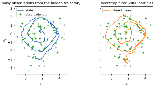
pp. 543–545 For a Markovian state-space model the target is the joint posterior of the states, \[ \pi_T(\bm z_{1:T})\propto p(\bm z_{1:T},\bm y_{1:T})=p(\bm z_1)p(\bm y_1\given\bm z_1)\prod_{t=2}^{T}p(\bm z_t\given\bm z_{t-1})p(\bm y_t\given\bm z_t), \tag{13.2} \] with the choice \(\tilde\gamma_t(\bm z_{1:t})=p(\bm z_{1:t},\bm y_{1:t})\) (13.3); it is a distribution over an ever longer sequence, but usually only its last marginal \(\tilde\gamma_t(\bm z_t)\) is needed, which avoids storing the history. (The book writes the product in (13.2) and (13.3) from \(t=1\) or \(s=1\), which counts the factors \(p(\bm y_1\given\bm z_1)\) and the first transition twice; the product starts at 2 as written here, see the notes on the book.) The book's running example is a 2-d nonlinear tracking problem, \[ p(\bm z_t\given\bm z_{t-1})=\N(\bm z_t\given\bm f(\bm z_{t-1}),q\bm I),\quad p(\bm y_t\given\bm z_t)=\N(\bm y_t\given\bm z_t,r\bm I),\quad \bm f(\bm z)=(z_1+\Delta\sin z_2,\;z_2+\Delta\cos z_1), \tag{13.4} \] filtered in Figure 13.1 by the simplest SMC algorithm, the bootstrap filter (Section 13.2.3.1). The point \((\pi/2,0)\) is a fixed point of \(\bm f\) whose Jacobian \(\begin{pmatrix}1&\Delta\\-\Delta&1\end{pmatrix}\) has eigenvalues \(1\pm i\Delta\) of modulus \(\sqrt{1+\Delta^2}>1\), so trajectories started near it spiral outward, which is the shape in the figure.
Particle filtering also applies to non-Markovian models, in which \(\bm z_t\) depends on the whole past and \(\bm y_t\) on \(\bm z_{1:t}\), with \[ \tilde\gamma_t(\bm z_{1:t})=p(\bm z_1)p(\bm y_1\given\bm z_1)\prod_{s=2}^t p(\bm z_s\given\bm z_{1:s-1})p(\bm y_s\given\bm z_{1:s}), \tag{13.5} \] for instance the 1-d Gaussian sequence model \[ p(z_t\given z_{1:t-1})=\N(z_t\given\phi z_{t-1},q),\qquad p(y_t\given z_{1:t})=\N\Big(y_t\,\Big|\,\sum_{s=1}^t\beta^{t-s}z_s,\;r\Big), \tag{13.6} \] which is a linear-Gaussian state-space model at \(\beta=0\) and becomes harder as \(\beta\) grows. It is used for Figures 13.2 and 13.3 below. Writing \(m_t=\sum_{s\le t}\beta^{t-s}z_s=\beta m_{t-1}+z_t\) shows that \((z_t,m_t)\) is a 2-d linear-Gaussian state, so the exact evidence is available from a Kalman filter; this is how the filters below are checked.
13.1.3 SMC samplers for static parameter estimation
p. 545 For a fixed data set \(\mathcal D=\{y_n\}_{n=1}^N\) with conditionally iid observations the posterior is \(p(\bm z\given\mathcal D)\propto p(\bm z)\prod_np(y_n\given\bm z)\): a single distribution, not a sequence. SMC makes a sequence out of it in two ways. In data tempering the target at step \(t\) uses the first \(t\) observations, \(\tilde\gamma_t(\bm z)=p(\bm z)p(\bm y_{1:t}\given\bm z)\), so \(T=N\). In likelihood tempering it is \(\tilde\gamma_t(\bm z)=p(\bm z)p(\mathcal D\given\bm z)^{\tau_t}\) with \(0=\tau_1<\dots<\tau_T=1\) (the book writes \(\tau_t=0\) for the first value; it is \(\tau_1\)). The marginal targets are then linked into targets over sequences by a backward kernel, which is the subject of Section 13.6.
13.2 Particle filtering
13.2.1 Importance sampling
pp. 545–546 To estimate \(\pi_t(\varphi)=\E_{\pi_t}[\varphi(\bm z_{1:t})]=\int\varphi\,\tilde\gamma_t/Z_t\) with a proposal \(q_t\), draw \(\bm z^i_{1:t}\overset{\mathrm{iid}}{\sim}q_t\) and form the unnormalised weights \(\tilde w^i_t=\tilde\gamma_t(\bm z^i_{1:t})/q_t(\bm z^i_{1:t})\) (13.9), the normaliser estimate \(\hat Z_t=\frac1{N_s}\sum_i\tilde w_t^i\) (13.10) and the normalised weights \(W_t^i=\tilde w_t^i/\sum_j\tilde w_t^j\) (13.11). The self-normalised estimate is \[ \pi_t(\varphi)\approx\frac1{\hat Z_t}\frac1{N_s}\sum_{i=1}^{N_s}\tilde w^i_t\varphi(\bm z^i_{1:t})=\sum_{i=1}^{N_s}W_t^i\varphi(\bm z_{1:t}^i),\qquad \pi_t\approx\hat\pi_t=\sum_iW^i_t\,\delta_{\bm z^i_{1:t}}. \tag{13.8, 13.12, 13.13} \] The difficulty in sequential problems is that the dimension grows with \(t\), so a single proposal over the whole sequence almost never lands where \(\pi_t\) has mass and a few weights dominate. (The fixed-dimension version of importance sampling is in Bishop 11.1.4, All of Statistics 24.3 and Chapter 11 of this course; what the book leaves open is how good the self-normalised estimate is.)
Filling the gap 13.1: consistency, bias and asymptotic variance of self-normalised importance sampling, and unbiasedness of \(\hat Z\) pp. 545–546, (13.8)–(13.13)
Derivation
Assumptions. \(q\) dominates \(\pi\) (\(q=0\) implies \(\tilde\gamma=0\)), \(w=\tilde\gamma/q\) has \(\E_q[w^2]<\infty\) and \(\E_q[w^2\varphi^2]<\infty\). Write \(A_N=\frac1N\sum_iw^i\varphi(z^i)\) and \(B_N=\hat Z=\frac1N\sum_iw^i\), \(z^i\) iid from \(q\).
Unbiasedness of \(\hat Z\). \(\E_q[w]=\int q\,\tilde\gamma/q=\int\tilde\gamma=Z\) (the support condition is used), so \(\E[B_N]=Z\) and \(\var(B_N)=\var_q(w)/N\) is finite by the second-moment assumption. This is the property that is inherited by SMC (gap 13.3).
Consistency. \(\E_q[w\varphi]=Z\pi(\varphi)\). By the strong law, \(A_N\to Z\pi(\varphi)\) and \(B_N\to Z\) almost surely, so \(\pi_N(\varphi)=A_N/B_N\to\pi(\varphi)\) almost surely (\(Z>0\)).
Asymptotic variance. Put \(\varphi_c=\varphi-\pi(\varphi)\). Then \[ \frac{A_N}{B_N}-\pi(\varphi)=\frac{A_N-\pi(\varphi)B_N}{B_N}=\frac{\frac1N\sum_iw^i\varphi_c(z^i)}{B_N}. \] The summands \(w^i\varphi_c(z^i)\) are iid with mean \(Z\pi(\varphi)-\pi(\varphi)Z=0\) and variance \(\E_q[w^2\varphi_c^2]\), so \(\sqrt N\) times the numerator converges in law to \(\N(0,\E_q[w^2\varphi_c^2])\) by the central limit theorem, while \(B_N\to Z\) in probability. Slutsky's lemma gives \[ \sqrt N\big(\pi_N(\varphi)-\pi(\varphi)\big)\Rightarrow\N\Big(0,\;\frac{\E_q[w^2(\varphi-\pi(\varphi))^2]}{Z^2}\Big). \] This is the delta method for the ratio \(g(a,b)=a/b\), whose gradient at \((Z\pi(\varphi),Z)\) is \((1/Z,-\pi(\varphi)/Z)\).
Bias. A second-order expansion of \(g\) gives \(\E[A_N/B_N]-\pi(\varphi)=\frac1N\,\big(\pi(\varphi)\var_q(w)-\cov_q(w\varphi,w)\big)/Z^2+o(1/N)\): the self-normalised estimate is biased, at the order \(1/N\), much smaller than the standard deviation \(O(N^{-1/2})\).
Numerical confirmation. For \(\pi=\N(0,1)\), \(q=\N(0,2^2)\), \(\varphi(z)=z^2\), \(N=400\), the formula gives an asymptotic variance that matches \(N\) times the variance observed over 4000 repetitions to within 1% (ratio 1.007), the mean of \(\hat Z\) is 1 up to simulation error, and the estimates of \(\E[z^2]=1\) average 0.9988.
See also: Bishop, 11.1.4 importance sampling; All of Statistics, 24.3.
13.2.2 Sequential importance sampling
pp. 547–548 Sequential importance sampling (SIS) gives the proposal an autoregressive structure, \(q_t(\bm z_{1:t})=q_{t-1}(\bm z_{1:t-1})\,q_t(\bm z_t\given\bm z_{1:t-1})\) (13.14): the old sequences are reused and "grown" by one step. The weights then obey a recursion, \[ \tilde w_t=\tilde w_{t-1}\,\alpha_t,\qquad \alpha_t(\bm z_{1:t})=\frac{\tilde\gamma_t(\bm z_{1:t})}{\tilde\gamma_{t-1}(\bm z_{1:t-1})\,q_t(\bm z_t\given\bm z_{1:t-1})}, \tag{13.17, 13.18} \] and, for a state-space model with \(\tilde\gamma_t=p(\bm z_{1:t},\bm y_{1:t})\), the incremental weight simplifies to \(\alpha_t=p(\bm y_t\given\bm z_{1:t})\,p(\bm z_t\given\bm z_{1:t-1})/q_t(\bm z_t\given\bm z_{1:t-1})\) (13.21). Algorithm 13.1 is this loop (in practice in log space with the log-sum-exp trick).
Algorithm 13.1 (Sequential importance sampling). For \(i=1{:}N_s\): draw \(\bm z_1^i\sim q_1\), set \(\tilde w^i_1=\tilde\gamma_1(\bm z_1^i)/q_1(\bm z_1^i)\). For \(t=2{:}T\) and each \(i\): draw \(\bm z^i_t\sim q_t(\cdot\given\bm z^i_{1:t-1})\), compute \(\alpha_t^i\) by (13.18), set \(\tilde w^i_t=\tilde w^i_{t-1}\alpha^i_t\); normalise to \(W^i_t\) and output \(\hat\pi_t=\sum_iW^i_t\delta_{\bm z^i_{1:t}}\).
Filling the gap 13.2: the weight recursion and why SIS degenerates pp. 547–548, (13.15)–(13.21), Figure 13.2
Derivation
Recursion. Insert (13.14) into the definition \(\tilde w_t=\tilde\gamma_t(\bm z_{1:t})/q_t(\bm z_{1:t})\) and multiply and divide by \(\tilde\gamma_{t-1}(\bm z_{1:t-1})\): \[ \tilde w_t=\frac{\tilde\gamma_{t-1}(\bm z_{1:t-1})}{q_{t-1}(\bm z_{1:t-1})}\cdot\frac{\tilde\gamma_t(\bm z_{1:t})}{\tilde\gamma_{t-1}(\bm z_{1:t-1})\,q_t(\bm z_t\given\bm z_{1:t-1})}=\tilde w_{t-1}\alpha_t. \] For a state-space model, \(p(\bm z_{1:t},\bm y_{1:t})=p(\bm y_t\given\bm z_{1:t})p(\bm z_t\given\bm z_{1:t-1})p(\bm z_{1:t-1},\bm y_{1:t-1})\) (chain rule, (13.19)), so the factor \(\tilde\gamma_{t-1}\) cancels in (13.18) and (13.21) follows. A direct numerical experiment on the non-Markovian model (13.6): for the dynamics as proposal, \(\log\tilde w_6\) computed as \(\log\tilde\gamma_6-\log q_6\) equals \(\sum_t\log p(y_t\given z_{1:t})\) to machine precision.
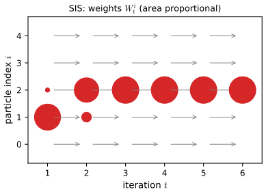
Degeneracy. Take the simplest case in which the target and the proposal factorise over time, \(\tilde\gamma_T/q_T=\prod_{s\le T}w(z_s)\) with \(w(z_s)>0\) iid under \(q\). Then \(\tilde w^i_T=\prod_sw(z^i_s)\) and, with \(\mu_k=\E_q[w^k]\), \[ \frac{N}{\mathrm{ESS}}=\frac{N\sum_i(\tilde w^i_T)^2}{(\sum_i\tilde w_T^i)^2}=\frac{\frac1N\sum_i(\tilde w^i_T)^2}{(\frac1N\sum_i\tilde w_T^i)^2}\;\xrightarrow[N\to\infty]{\text{a.s.}}\;\frac{\E_q[w^2]^T}{\E_q[w]^{2T}}=\rho^{T},\qquad \rho=\frac{\mu_2}{\mu_1^2}. \] By Jensen's (or Cauchy–Schwarz) inequality \(\rho\ge1\) with equality only if \(w\) is constant. Hence \(\mathrm{ESS}/N\to\rho^{-T}\) decays geometrically in \(T\): to keep a fixed ESS the number of particles must grow like \(\rho^T\). Numerically, for \(\pi=\N(0,1)^T\) and \(q=\N(0,1.5^2)^T\) one finds \(N/\mathrm{ESS}=1.203,\,1.448,\,1.740\) for \(T=1,2,3\) against \(\rho^T=1.203,\,1.448,\,1.743\). The reason for the explosion is that \(\log\tilde w_T\) is a sum of \(T\) iid terms, a random walk with a negative drift and fluctuations of order \(\sqrt T\), so the ratios between different particles' weights spread out like a log-normal with variance proportional to \(T\); eventually the largest weight dwarfs the rest (Figure 13.2a).
13.2.3 Sequential importance sampling with resampling
pp. 548–549 The cure is to resample: instead of growing every old sequence, first select \(N_s\) survivors by sampling from the old weighted approximation, then grow them. At step \(t\) the proposal is \[ q^{\mathrm{SISR}}_t(\bm z_{1:t})=\hat\pi_{t-1}(\bm z_{1:t-1})\,q_t(\bm z_t\given\bm z_{1:t-1}) \tag{13.22} \] (whereas SIS uses \(q_{t-1}^{\mathrm{SIS}}\) in the first factor, (13.23)). It is sampled in two steps: resample \(N_s\) ancestors from \(\hat\pi_{t-1}\) (Section 13.2.4) to get an equally weighted set, then extend each by \(\bm z_t^i\sim q_t\). The weights are computed as if the proposal were \(\tilde\gamma_{t-1}q_t\), so, since resampling resets the old weights to one, the new unnormalised weight is just the incremental weight \(\alpha_t\).
Algorithm 13.2 (SISR). Initialise as in Algorithm 13.1. For \(t=2{:}T\): compute ancestors \(a_{t-1}^{1:N_s}=\mathrm{resample}(\tilde w^{1:N_s}_{t-1})\); select \(\bm z^{1:N_s}_{1:t-1}\leftarrow\bm z^{a^{1:N_s}}_{1:t-1}\); reset \(\tilde w^{1:N_s}_{t-1}=1/N_s\); draw \(\bm z_t^i\sim q_t(\cdot\given\bm z_{1:t-1}^i)\); set \(\tilde w^i_t=\alpha^i_t\) from (13.18); normalise and output \(\hat\pi_t\).
Filling the gap 13.3: why SISR is valid and why \(\hat Z_T\) is unbiased pp. 548–550, (13.22)–(13.28); Supplement (13.2)
Derivation
The book says the "pretend" proposal is valid because \(\hat\pi_{t-1}\) is an unbiased estimate of the previous target, and the supplement states \(\E[\hat Z_t]=Z_t\) with a pointer to the literature. Here is a complete argument for multinomial resampling at every step; the same statement holds for any unbiased resampling scheme (gap 13.5) and for adaptive resampling (the decision to resample depends only on the past), which the numerical experiments below confirm.
Set-up. Let \(\alpha^i_t\) be the incremental weights of Algorithm 13.2 and \(\hat Z_t=\prod_{s\le t}\big(\frac1{N}\sum_i\alpha_s^i\big)\) (this is (13.26)–(13.28), since \(\tilde w_s^i=\alpha_s^i\) after the reset). For \(t\ge1\) and a bounded measurable \(f\) of \(\bm z_{1:t}\) define \[ \hat\Gamma_t(f)=\hat Z_{t-1}\;\frac1N\sum_{i=1}^N\alpha_t^i\,f(\bm z^i_{1:t}),\qquad \hat Z_0=1. \] Claim: \(\E[\hat\Gamma_t(f)]=\int\tilde\gamma_t f\,\d\bm z_{1:t}\) for all \(t\) and \(f\). Taking \(f\equiv1\): \(\hat\Gamma_t(1)=\hat Z_t\) and so \(\E[\hat Z_t]=Z_t\).
Proof by induction. For \(t=1\) this is plain importance sampling, \(\E[\alpha_1f]=\int q_1(\tilde\gamma_1/q_1)f\). Assume the claim at \(t-1\) for all test functions. Condition on \(\mathcal F_{t-1}\), everything generated up to the weights at step \(t-1\). The ancestors \(a^i\) are iid with \(\Pr(a^i=j)=W^j_{t-1}=\alpha_{t-1}^j/\sum_k\alpha^k_{t-1}\), and given the ancestor \(\bm z^i_t\sim q_t(\cdot\given\bm z^{a^i}_{1:t-1})\). Hence, with \(h(\bm z_{1:t-1})=\int\tilde\gamma_t(\bm z_{1:t-1},z_t)f(\bm z_{1:t-1},z_t)\,\d z_t\) and the identity \(q_t\alpha_t=\tilde\gamma_t/\tilde\gamma_{t-1}\), \[ \E\Big[\frac1N\sum_i\alpha_t^if(\bm z_{1:t}^i)\,\Big|\,\mathcal F_{t-1}\Big]=\sum_jW^j_{t-1}\int q_t\,\alpha_t\,f\,\d z_t=\sum_jW_{t-1}^j\frac{h(\bm z^j_{1:t-1})}{\tilde\gamma_{t-1}(\bm z^j_{1:t-1})}. \] Multiply by the \(\mathcal F_{t-1}\)-measurable \(\hat Z_{t-1}=\hat Z_{t-2}\frac1N\sum_k\alpha^k_{t-1}\): the product \(\hat Z_{t-1}W_{t-1}^j=\hat Z_{t-2}\alpha^j_{t-1}/N\), so \[ \E[\hat\Gamma_t(f)\given\mathcal F_{t-1}]=\hat Z_{t-2}\frac1N\sum_j\alpha^j_{t-1}\,g(\bm z^j_{1:t-1})=\hat\Gamma_{t-1}(g),\qquad g=\frac{h}{\tilde\gamma_{t-1}}. \] Taking expectations and applying the induction hypothesis to \(g\): \(\E[\hat\Gamma_t(f)]=\int\tilde\gamma_{t-1}\,g=\int h=\int\tilde\gamma_tf\). \(\square\)
Consequences. (i) \(\E[\hat Z_t]=Z_t\): the evidence estimate (13.26) is unbiased although the normalised estimates \(\sum_iW^i_t\varphi\) are only consistent. (ii) Unbiasedness is exact for every \(N\), including \(N=2\): on a two-state hidden Markov model with three observations (all \(2^3\) paths enumerable) the average of \(\hat Z\) over 300000 runs with \(N=2\) was 0.9993 times \(Z\). (iii) On the non-Markovian model (13.6) with \(T=10\), 3000 runs with 100 particles gave \(\E[\hat Z]/Z=1.0005\pm0.027\) (multinomial, resampling every step) and \(1.016\pm0.027\) (systematic, adaptive resampling); the SIS estimate is also unbiased but so skewed that its median is below 1% of \(Z\). (iv) The expected logarithm is not the log of the expectation: by Jensen \(\E\log\hat Z_T\le\log Z_T\), used in Section 13.6.7.
13.2.3.1 Bootstrap filter
p. 549 For a state-space model, take the dynamics as the proposal, \(q_t(\bm z_t\given\bm z_{1:t-1})=p(\bm z_t\given\bm z_{1:t-1})\) (13.24). Then (13.21) gives \(\alpha_t=p(\bm y_t\given\bm z_t)\) in the Markov case (more generally \(p(\bm y_t\given\bm z_{1:t})\), (13.25)): propagate each particle through the dynamics, weight by the likelihood, resample. This is the bootstrap filter (Gordon et al. 1993), also called survival of the fittest and, in computer vision, condensation. It needs only a sampler of the dynamics, not their density, which is why it is used for simulators defined by differential equations; but it ignores \(\bm y_t\) when proposing, which is inefficient when the observation is informative (Section 13.3). Demonstration: the bootstrap filter against the exact Kalman filter (presets 1, 4 and 7, the last the spiral of Figure 13.1).
13.2.3.2 Path degeneracy problem
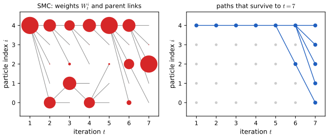
p. 550 Resampling removes weight degeneracy (Figure 13.3a: the weights stay balanced and the population turns over) but causes path degeneracy: when the whole path \(\bm z_{1:t}\) is of interest, the surviving paths share their early history, because resampling copies parents. In Figure 13.3b all five final paths trace back to one particle at time 1. The time at which all lineages meet is the coalescence time.
Filling the gap 13.4: how fast do the lineages coalesce? p. 550
Derivation
Look at two distinct particles at step \(t\) and ask whether they have the same parent at step \(t-1\). With ancestors drawn iid from the weights \(W^1,\dots,W^N\) (multinomial resampling), the probability that two given particles pick the same parent is \(\sum_jW_j^2=1/\mathrm{ESS}\) (gap 13.6). With equal weights it is \(1/N\). If this probability is constant, the number of generations one has to go back until the two lineages merge is geometric with success probability \(1/\mathrm{ESS}\), mean \(\mathrm{ESS}\le N\). Therefore the expected coalescence time of two lineages is of order \(\mathrm{ESS}\) steps (for \(N\) iid-uniform parents it is exactly \(N\), the Wright–Fisher result), and after \(T\gg N\) steps the whole population shares one ancestor at time 1; a smoothing estimate of \(\bm z_1\) from a particle filter is then just a single point. The estimate of the current state \(\bm z_t\) is not affected. In the demonstration, 500 particles resampled at every step for \(T=100\) leave only 4 distinct time-1 ancestors among the final particles (preset 1), while without resampling (preset 2) all 500 remain and the weights have collapsed instead: the two pathologies trade off, which is what adaptive resampling (Section 13.2.5) balances.
13.2.3.3 Estimating the normalizing constant
pp. 550–551 Because \(Z_T=p(\bm y_{1:T})=\prod_tp(\bm y_t\given\bm y_{1:t-1})\), the particle filter gives \[ \hat Z_T=\prod_{t=1}^T\hat Z_t\big/\hat Z_{t-1},\qquad \widehat{Z_t/Z_{t-1}}=\frac{\sum_i\tilde w^i_t}{\sum_i\tilde w^i_{t-1}}, \tag{13.26–13.28} \] the product of the mean incremental weights (with resampling at every step the denominator is 1 after the reset convention \(\tilde w=1/N_s\)). It is an unbiased estimate of the marginal likelihood (gap 13.3), which makes the particle filter usable for parameter estimation (Section S13.2). In the demonstration the estimate is shown next to the exact Kalman log-evidence; without resampling (SIS) it is far too small in a typical run (\(-137.9\) against \(-97.7\) in preset 2), although unbiased on average over runs.
13.2.4 Resampling methods
pp. 551–553 Given a weighted set \(\{(W^i,\bm z^i)\}\), draw ancestors \(A^1,\dots,A^N\) and keep \(\bm z^{A^1},\dots,\bm z^{A^N}\) with equal weights \(1/N\). If a single index has \(\Pr(A=i)=W^i\) then \(\E[f(\bm z^A)]=\sum_iW^if(\bm z^i)\) (13.30), and for \(N\) independent indices \(\E_{A_{1:N}}\big[\frac1N\sum_jf(\bm z^{A_j})\big]=\sum_iW^if(\bm z^i)\) (13.32): the resampled set gives the same expectation as the weighted one but drops low-weight particles and duplicates high-weight ones. What differs between schemes is the variance. Most schemes work by the inverse cdf: form the cumulative weights \(c_a=\sum_{j\le a}W^j\) (the staircase of Figure 13.4), take points \(U^1\le\dots\le U^N\) in \((0,1)\), and send \(U^i\) to the index \(a\) with \[ c_{a-1}\le U^i<c_a. \tag{13.33} \] Sorted points make this an \(O(N)\) sweep instead of \(O(N^2)\) (Listing 13.1 in the book does it with a binary search).
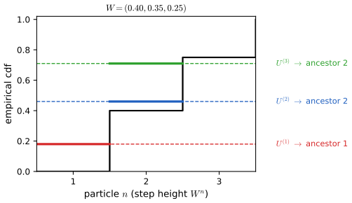
- 13.2.4.2 Multinomial: \(U^{1:N}\) are the order statistics of \(N\) iid uniforms. With equal weights the number of offspring of one particle is \(\mathrm{Bin}(N,1/N)\), so it has none with probability \((1-1/N)^N\to e^{-1}\approx0.37\): more than a third of the particles vanish although all were equally good.
- 13.2.4.3 Stratified: \(U^i\sim\mathrm{Unif}((i-1)/N,i/N)\) independently, one point in each stratum (13.34).
- 13.2.4.4 Systematic: \(U^i=\frac{i-1}N+\frac uN\) with one shared \(u\sim\mathrm{Unif}(0,1)\) (13.35): an evenly spaced comb shifted at random.
- 13.2.4.5 Comparison: all are unbiased; multinomial has provably larger variance and is not recommended; systematic is empirically the best (Hol et al. 2006) although stratified (and the scheme of Gerber et al. 2019) have better theoretical properties.
Filling the gap 13.5: unbiasedness and the offspring variances of the resampling schemes pp. 551–553, (13.30)–(13.35)
Derivation
Let \(O_n=\#\{i:A^i=n\}\) be the number of offspring of particle \(n\), and \(I_n=[c_{n-1},c_n)\) its interval, of length \(W^n\). Since \(\frac1N\sum_jf(\bm z^{A_j})=\frac1N\sum_nO_nf(\bm z^n)\), every scheme with \(\E[O_n]=NW^n\) is unbiased in the sense of (13.32).
Multinomial. \((O_1,\dots,O_N)\sim\mathrm{Mult}(N,W)\), so \(O_n\sim\mathrm{Bin}(N,W^n)\): mean \(NW^n\), variance \(NW^n(1-W^n)\), and \(\Pr(O_n=0)=(1-W^n)^N\). With \(W^n=1/N\) this is \((1-1/N)^N\), which decreases to \(e^{-1}=0.3679\) (0.358 for \(N=20\), 0.3676 for \(N=2000\) in simulation).
Systematic. The points \(U^i=(i-1+u)/N\) form a lattice of spacing \(\delta=1/N\). A half-open interval of length \(\ell\) contains \(\lfloor\ell/\delta\rfloor\) or \(\lceil\ell/\delta\rceil\) lattice points, whatever its position. So \(O_n\in\{\lfloor NW^n\rfloor,\lceil NW^n\rceil\}\). Also \(\E[O_n]=\sum_i\Pr(U^i\in I_n)=\sum_i N|I_n\cap[\tfrac{i-1}N,\tfrac iN)|=NW^n\) (each \(U^i\) is uniform on its stratum). A variable on \(\{k,k+1\}\) with mean \(k+\theta\) (\(\theta=\mathrm{frac}(NW^n)\)) has variance \(\theta(1-\theta)\le\tfrac14\). In particular with equal weights every particle receives exactly one offspring.
Stratified. The point of stratum \(k=[\tfrac{k-1}N,\tfrac kN)\) falls in \(I_n\) with probability \(p_{nk}=N|I_n\cap\text{stratum }k|\), independently over \(k\). So \(O_n=\sum_k\mathrm{Bernoulli}(p_{nk})\), with \(\E O_n=\sum_kp_{nk}=NW^n\) and \(\var(O_n)=\sum_kp_{nk}(1-p_{nk})\). A stratum inside \(I_n\) has \(p=1\), one disjoint from it \(p=0\); at most two strata (those containing the endpoints of \(I_n\)) overlap it partially, so \(\var(O_n)\le\tfrac14+\tfrac14=\tfrac12\). The exact value is what the demonstration plots.
Comparison. Per particle, multinomial \(NW(1-W)\) grows with \(N\) for a fixed \(W\) scale, whereas systematic is at most 1/4 and stratified at most 1/2. For 20 particles with log-normal weights (\(W^n\propto e^{g_n}\), \(g_n\) standard normal) the exact total offspring variance \(\sum_n\var O_n\) is 18.3 for multinomial, 5.9 for stratified and 3.7 for systematic (the demonstration shows the same ordering and lets one change the weights). A caveat: the variance of the resampled estimate \(\frac1N\sum_nO_nf(\bm z^n)\) also involves the covariances between the \(O_n\), and for systematic resampling these depend on the order of the particles (the points are strongly negatively correlated for neighbours); the figure below randomises the order, and the ranking multinomial \(>\) stratified \(>\) systematic persisted (standard deviations 0.031, 0.017, 0.014 at \(N=1000\)).
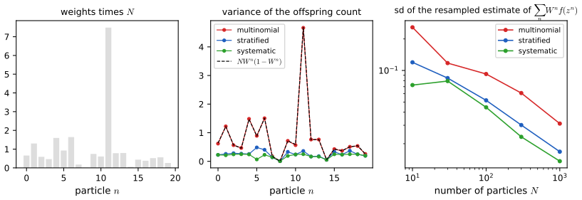
Demonstration: resampling schemes draws the staircase and the ancestors for any weights and compares exact and simulated offspring variances (presets 1 (equal weights: who disappears?), 3).
13.2.5 Adaptive resampling
p. 553 Resampling at every step loses diversity (path degeneracy), never resampling is SIS (weight degeneracy); a compromise resamples only when the effective sample size falls below a threshold, typically \(N/2\): \[ \mathrm{ESS}(W^{1:N})=\frac1{\sum_n(W^n)^2},\qquad \mathrm{ESS}(\tilde w^{1:N})=\frac{(\sum_n\tilde w^n)^2}{\sum_n(\tilde w^n)^2}. \tag{13.36, 13.37} \] (Murphy notes that this ESS differs from the MCMC one, which accounts for autocorrelation.) Algorithm 13.3 (SISR with adaptive resampling, the generic SMC algorithm): for \(t=1{:}T\), propose \(\bm z_t^i\sim q_t\), compute \(\alpha_t^i\), set \(\tilde w_t^i=\tilde w_{t-1}^i\alpha_t^i\), update \(\hat Z_t=\hat Z_{t-1}\sum_i\tilde w^i_t/\sum_i\tilde w^i_{t-1}\); if \(\mathrm{ESS}(\tilde w_t)<\mathrm{ESS}_{\min}\), resample and reset the weights to \(1/N\); then normalise (the book writes the test on \(\tilde w_{t-1}\); as the text says "resample when the ESS drops", the weights just computed are meant, see the notes on the book).
Filling the gap 13.6: properties of the effective sample size p. 553, (13.36), (13.37)
Derivation
(13.36) equals (13.37). With \(W^n=\tilde w^n/S\), \(S=\sum_n\tilde w^n\): \(1/\sum(W^n)^2=S^2/\sum(\tilde w^n)^2\).
Range. By Cauchy–Schwarz, \((\sum_nW^n\cdot1)^2\le N\sum_n(W^n)^2\), i.e. \(\mathrm{ESS}\le N\) with equality iff all weights are equal; and \(\sum(W^n)^2\le(\sum W^n)^2=1\) (all terms nonnegative), so \(\mathrm{ESS}\ge1\), with equality iff one weight is 1. If \(k\) weights equal 1 and \(N-k\) are 0, \(\mathrm{ESS}=k^2/k=k\).
Relation to the spread of the weights. Let \(\bar w=\frac1N\sum\tilde w^n\) and \(s^2=\frac1N\sum(\tilde w^n-\bar w)^2\). Then \(\sum(\tilde w^n)^2=N(s^2+\bar w^2)\), so \[ \mathrm{ESS}=\frac{N^2\bar w^2}{N(s^2+\bar w^2)}=\frac N{1+\mathrm{CV}^2},\qquad\mathrm{CV}=\frac s{\bar w}. \] The ESS is the number of equally weighted samples with the same weight dispersion. For iid weights \(N/\mathrm{ESS}\to\E[w^2]/\E[w]^2=1+\mathrm{CV}^2\), so (compare gap 13.1) the asymptotic variance of self-normalised importance sampling is that of an iid sample of size \(\mathrm{ESS}\) when \(\varphi\) is roughly independent of \(w\) (Kong's heuristic).
Link to path degeneracy. \(1/\mathrm{ESS}=\sum_n(W^n)^2\) is the probability that two multinomial draws pick the same parent (gap 13.4).
S13.1 More applications of particle filtering (supplement)
Supp. pp. 149–152 The supplement gives four applications of the bootstrap filter.
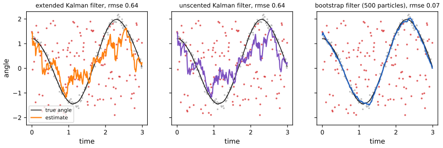
S13.1.1 A pendulum with outliers. The angle of a pendulum is observed through a sensor that, with probability 0.4, returns garbage drawn uniformly from \((-2,2)\). Deterministic filters assume a Gaussian posterior and are dragged by the outliers; the bootstrap filter, whose likelihood is the true two-component mixture, keeps a multimodal belief about which readings to trust. Figure S13.1 shows this with my own pendulum constants (the book's pendulum is from its Section 8.2.2).
S13.1.2 Visual object tracking (image sequences, a colour-histogram likelihood and about 250 particles) shows both the strength of the method (a bimodal posterior when a grey building looks like the grey helicopter) and its failure mode: the belief can lock onto the wrong mode, after which recovery from the proposals is unlikely; more particles or proposals from an object detector ("tracking by detection", Section 13.3) help. These figures are photographs and are not reproduced.
S13.1.3 Online parameter estimation. Treating a static parameter \(\bm\theta\) as part of the state with the "dynamics" \(p(\bm\theta_t\given\bm\theta_{t-1})=\delta(\bm\theta_t-\bm\theta_{t-1})\) does not work; adding artificial noise cures the collapse but washes out the prior and discounts old data. The SMC sampler of Section 13.6.3 (data tempering with rejuvenation moves) is the remedy.
Filling the gap 13.17: a particle filter for a static parameter collapses Supp. p. 151, Section S13.1.3
Derivation
With zero system noise the propagation step does nothing: each particle carries a fixed value \(\theta^i\), only the weights change. Resampling then only copies existing values. Let \(D_t\) be the number of distinct values among the \(N\) particles after step \(t\). Each resampling step can only copy, never create, values, so \(D_{t+1}\le D_t\). Moreover, as long as the weights are strictly positive (a Gaussian likelihood is), with probability at least \(\prod_{i=1}^N W^{i^*}>0\) all \(N\) ancestors are the same particle \(i^*\), so \(D=1\) is reachable from any state in one step. A finite Markov chain with a nonincreasing statistic and an absorbing state reachable from everywhere is absorbed almost surely: \(D_t\to1\), i.e. the posterior approximation collapses to a single point, however large \(N\) is; the posterior spread is lost entirely, not merely approximated badly. In a simulation with \(N=500\) particles for the mean of a \(\mathcal N(\theta,1)\) sample, the number of distinct values fell monotonically from 500 to 10 after 60 observations. Artificial noise would add new values but biases the posterior; the SMC-sampler remedy adds MCMC moves that leave the current posterior invariant (gap 13.12).
S13.1.4 Monte Carlo robot localisation. A robot with a known occupancy-grid map and a range sensor estimates where it is. The exact HMM filter costs \(O(K^2)\) per step for \(K\) grid cells; a particle filter is a sparse approximation of the belief. Starting from a uniform prior (global localisation) the cloud first spreads over every corridor, then, as the sensor sees more, contracts; perceptual aliasing (different places that look alike) keeps several clusters alive until a distinguishing observation arrives. The accompanying figure is from Thrun et al. (2006) and is not reproduced.
13.3 Proposal distributions
p. 553 The efficiency of a particle filter depends on the proposal: the bootstrap proposal ignores the newest observation, so with a precise sensor almost all particles are proposed where the likelihood is negligible. The remedy is a proposal that uses \(\bm y_t\).
13.3.1 Locally optimal proposal
p. 554 The one-step locally optimal proposal minimises \(\KL\big(\pi_{t-1}(\bm z_{1:t-1})q_t(\bm z_t\given\bm z_{1:t-1})\,\|\,\pi_t(\bm z_{1:t})\big)\) (13.38) and is \[ q_t^*(\bm z_t\given\bm z_{1:t-1})=\pi_t(\bm z_t\given\bm z_{1:t-1})=\frac{\tilde\gamma_t(\bm z_{1:t})}{\tilde\gamma_t(\bm z_{1:t-1})},\qquad\tilde\gamma_t(\bm z_{1:t-1})=\int\tilde\gamma_t\,\d\bm z_t, \tag{13.42} \] which for a state-space model is \(p(\bm z_t\given\bm z_{1:t-1},\bm y_{1:t})\): condition on all the data including \(\bm y_t\) (a guided particle filter). It is usually intractable, hence the approximations below.
Filling the gap 13.7: the locally optimal proposal minimises the KL and has constant incremental weight p. 554, (13.38)–(13.42)
Derivation
Factor the target as \(\pi_t(\bm z_{1:t})=\pi_t(\bm z_{1:t-1})\pi_t(\bm z_t\given\bm z_{1:t-1})\), where \(\pi_t(\bm z_{1:t-1})=\tilde\gamma_t(\bm z_{1:t-1})/Z_t\) is the marginal. Then \[ \KL(\pi_{t-1}q_t\|\pi_t)=\E_{\pi_{t-1}q_t}\Big[\log\frac{\pi_{t-1}(\bm z_{1:t-1})}{\pi_t(\bm z_{1:t-1})}+\log\frac{q_t(\bm z_t\given\bm z_{1:t-1})}{\pi_t(\bm z_t\given\bm z_{1:t-1})}\Big]=C+\E_{\pi_{t-1}}\big[\KL\big(q_t(\cdot\given\bm z_{1:t-1})\,\|\,\pi_t(\cdot\given\bm z_{1:t-1})\big)\big], \] where \(C=\E_{\pi_{t-1}}\log(\pi_{t-1}/\pi_t(\bm z_{1:t-1}))\) does not involve \(q_t\) (this is (13.39)–(13.41)). The second term is a mean of nonnegative KL divergences, zero iff \(q_t=\pi_t(\cdot\given\bm z_{1:t-1})\) for \(\pi_{t-1}\)-almost every past, which proves (13.42).
Weights. With \(q_t=\pi_t(\bm z_t\given\bm z_{1:t-1})=\tilde\gamma_t(\bm z_{1:t})/\tilde\gamma_t(\bm z_{1:t-1})\) the incremental weight (13.18) is \[ \alpha_t=\frac{\tilde\gamma_t(\bm z_{1:t})}{\tilde\gamma_{t-1}(\bm z_{1:t-1})}\cdot\frac{\tilde\gamma_t(\bm z_{1:t-1})}{\tilde\gamma_t(\bm z_{1:t})}=\frac{\tilde\gamma_t(\bm z_{1:t-1})}{\tilde\gamma_{t-1}(\bm z_{1:t-1})}, \] which does not depend on the new state \(\bm z_t\): given the past, all particles extended from it get the same weight, so the variance of the weights conditional on the past is zero, the smallest possible. For a Markov state-space model it equals \(p(\bm y_t\given\bm z_{t-1})\), the predictive likelihood. A numerical example (one linear-Gaussian step): five draws from the optimal proposal \(\N\big(\sigma^2(\mu/s_x+y/r),\sigma^2\big)\) with \(\sigma^{-2}=1/s_x+1/r\) all gave the incremental weight \(\N(y\given\mu,s_x+r)\) to machine precision.
13.3.2 Proposals based on the extended and unscented Kalman filter
p. 555 For \(\bm z_t=\bm f(\bm z_{t-1})+\bm q_t\), \(\bm y_t=\bm h(\bm z_t)+\bm r_t\), approximate, for each particle \(i\), the joint of neighbouring state and observation given the history as Gaussian, \[ p(\bm z_t,\bm y_t\given\bm z^i_{1:t-1})\approx\N\Big(\begin{pmatrix}\bm z_t\\\bm y_t\end{pmatrix}\Big|\hat{\bm\mu}^i,\hat{\bm\Sigma}^i\Big),\tag{13.43, 13.44} \] with \(\hat{\bm\mu}^i,\hat{\bm\Sigma}^i\) computed by linearising \(\bm f,\bm h\) (extended Kalman filter, giving the extended particle filter) or by propagating sigma points (unscented, giving the unscented particle filter), and then condition: \[ q(\bm z_t\given\bm z^i_{1:t-1},\bm y_t)=\N(\bm z_t\given\bm\mu^i_t,\bm\Sigma^i_t),\quad\bm\mu^i_t=\hat{\bm\mu}^i_z+\hat{\bm\Sigma}^i_{zy}(\hat{\bm\Sigma}^i_{yy})^{-1}(\bm y_t-\hat{\bm\mu}^i_y),\quad\bm\Sigma^i_t=\hat{\bm\Sigma}^i_{zz}-\hat{\bm\Sigma}^i_{zy}(\hat{\bm\Sigma}^i_{yy})^{-1}\hat{\bm\Sigma}^i_{yz}. \tag{13.45–13.47} \] The approximation is made separately for every particle. The importance weights are still computed with the exact densities, so any error in the Gaussian approximation costs efficiency, never correctness.
13.3.3 Proposals based on the Laplace approximation
pp. 555–556 For non-Gaussian observations (e.g. a GLM likelihood) with linear-Gaussian dynamics, find \(\bm z_t^*=\argmax\log p(\bm y_t\given\bm z_t)\) by Newton–Raphson and approximate the likelihood as a function of \(\bm z_t\) by \(\N(\bm z_t\given\bm z_t^*,-\bm H_t^{*-1})\) (13.48), \(\bm H_t^*\) the Hessian of the log likelihood at the mode; combining this with the Gaussian dynamics by a Kalman update gives the proposal: the Laplace Gaussian filter (Koyama et al. 2010).
Filling the gap 13.8: the Gaussian and Laplace proposals, derived pp. 555–556, (13.43)–(13.48)
Derivation
Conditioning (13.45)–(13.47). If \((\bm z,\bm y)\) is jointly Gaussian with the block mean and covariance of (13.44), then \(\bm z\given\bm y\) is Gaussian with mean \(\hat{\bm\mu}_z+\hat{\bm\Sigma}_{zy}\hat{\bm\Sigma}_{yy}^{-1}(\bm y-\hat{\bm\mu}_y)\) and covariance \(\hat{\bm\Sigma}_{zz}-\hat{\bm\Sigma}_{zy}\hat{\bm\Sigma}_{yy}^{-1}\hat{\bm\Sigma}_{yz}\): this is the conditioning formula proved in gap 2.10 (block inverse). For the EKF with \(\bm f,\bm h\) linearised at the particle, \(\hat{\bm\Sigma}\) is exactly the joint covariance of the linearised model, so (13.45) is the Kalman filter update.
Laplace proposal. Let the prior move be \(\N(\bm z_t\given\bm\mu_i,\bm Q)\) with \(\bm\mu_i=\bm F\bm z^i_{t-1}\), and the Laplace likelihood \(\N(\bm z_t\given\bm z_t^*,\bm P_L^{-1})\) with \(\bm P_L=-\bm H^*_t\succ0\). The product of two Gaussian densities in \(\bm z_t\) is proportional to a Gaussian with precision the sum of the precisions and mean the precision-weighted average (gap 2.12): \[ q(\bm z_t\given\bm z^i_{t-1},\bm y_t)=\N\big(\bm z_t\,\big|\,\bm\Sigma_p(\bm Q^{-1}\bm\mu_i+\bm P_L\bm z^*_t),\;\bm\Sigma_p\big),\qquad\bm\Sigma_p=(\bm Q^{-1}+\bm P_L)^{-1}. \] The same density is the Kalman update that treats \(\bm z^*_t\) as an observation of \(\bm z_t\) with noise covariance \(\bm P_L^{-1}\), which is the "update step of the Kalman filter" in the text. For a Poisson GLM, \(\log\lambda_k=\alpha_k+\bm\beta_k^\T\bm z\), the log likelihood \(\sum_k y_k(\alpha_k+\bm\beta_k^\T\bm z)-\lambda_k(\bm z)\) has gradient \(\sum_k(y_k-\lambda_k)\bm\beta_k\) and Hessian \(-\sum_k\lambda_k\bm\beta_k\bm\beta_k^\T\), negative definite whenever the \(\bm\beta_k\) span \(\R^6\), so Newton's method (with the same Hessian) is well defined; the mode found in the example had gradient below \(10^{-6}\). The weight is then \(p(\bm y_t\given\bm z_t)\,\N(\bm z_t\given\bm\mu_i,\bm Q)/q(\bm z_t\given\cdot)\), exact whatever the quality of the approximation.
13.3.3.1 Example: neural decoding
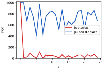
p. 556 A monkey moves its hand; \(\bm z_t\in\R^6\) holds 3-d position and velocity, each coordinate following a discretised integrated Brownian motion, \(\begin{pmatrix}z_t(i)\\z_t(i+3)\end{pmatrix}\sim\N\big(\begin{pmatrix}1&\Delta\\0&1\end{pmatrix}\bm z_{t-1},\sigma^2\bm Q\big)\) with \(\bm Q=\begin{pmatrix}\Delta^3/3&\Delta^2/2\\\Delta^2/2&\Delta\end{pmatrix}\) (13.49, 13.50), observed through the spike counts of \(K\) neurons, \(y_t(k)\sim\mathrm{Poisson}(\lambda_k(\bm z_t))\), \(\log\lambda_k=\alpha_k+\bm\beta_k^\T\bm z_t\) (13.51, 13.52). With 50 neurons the likelihood is far more informative than the dynamics, so the bootstrap filter's weights degenerate while the Laplace-guided filter keeps its ESS close to \(N\) (Figure 13.5). Both filters, run with enough particles, estimate the same evidence (\(-3472.4\) with 20000 bootstrap particles, \(-3472.7\) with 5000 guided particles).
13.3.4 Proposals based on SMC (nested SMC)
p. 557 SMC can itself compute the proposal: for each particle \(i\), run an inner SMC whose target is the optimal proposal \(p(\bm z_t\given\bm z^i_{1:t-1},\bm y_{1:t})\) (Naesseth et al. 2015, 2019). It needs no parametric assumption and so can approximate the optimal proposal arbitrarily well, at the price of speed (the inner runs are parallel across the outer particles).
13.4 Rao-Blackwellized particle filtering (RBPF)
p. 556 If the hidden variables split into \(\bm m_t\) and \(\bm z_t\) such that \(\bm z_t\) can be integrated out analytically given \(\bm m_{1:t}\), it suffices to sample \(\bm m_{1:t}\) and to carry a parametric belief about \(\bm z_t\) in each particle ("distributional" or "collapsed" particles): particle filtering for the awkward part, Kalman filtering for the rest. Sampling in a lower-dimensional space reduces the variance; this is Rao-Blackwellisation (the general statement is in Chapter 11 and gap 6.3).
13.4.1 Mixture of Kalman filters
pp. 557–558 The model is a switching linear dynamical system with discrete regime \(m_t\) and continuous state \(\bm z_t\): \[ p(\bm z_t\given\bm z_{t-1},m_t=k)=\N(\bm z_t\given\bm F_k\bm z_{t-1},\bm Q_k),\quad p(\bm y_t\given\bm z_t,m_t=k)=\N(\bm y_t\given\bm H_k\bm z_t,\bm R_k),\quad p(m_t=k\given m_{t-1}=j)=A_{jk}. \tag{13.53–13.55} \] Exact inference is intractable (the number of regime histories grows as \(K^t\)), but given a sampled history \(m^n_{1:t}\) a Kalman filter per particle computes the Gaussian \(\N(\bm z_t\given\bm\mu^n_t,\bm\Sigma^n_t)\) exactly, giving the belief \(p(\bm z_t,m_t\given\bm y_{1:t})\approx\sum_nW^n_t\,\delta(m_t-m_t^n)\,\N(\bm z_t\given\bm\mu^n_t,\bm\Sigma^n_t)\) (13.56). With the prior \(q(m_t\given m^n_{t-1})=p(m_t\given m_{t-1}^n)\) as proposal the weight update is \(\tilde w_t^n=\tilde w^n_{t-1}L^n_{tk}\) where \(L^n_{tk}=p(\bm y_t\given m_t=k,m^n_{1:t-1},\bm y_{1:t-1})\) (13.63, 13.64) is the Kalman filter's normalising constant (predictive density of \(\bm y_t\)). Algorithm 13.4 (one RBPF step): for each particle, sample \(k\sim p(m_t\given m^n_{t-1})\), run the Kalman update to get \((\bm\mu^n_t,\bm\Sigma^n_t,L^n_{tk})\), multiply the weight by \(L^n_{tk}\); resample (and reset weights) if the ESS is low.
Filling the gap 13.9: why Rao-Blackwellisation helps, the weight recursion and the Kalman predictive density pp. 556–559, (13.57)–(13.64)
Derivation
Variance reduction. Compare two importance samplers for the target \(p(m,z\given y)\): sample \((m,z)\) from \(q(m)q(z\given m)\) with weight \(w(m,z)=p(m,z,y)/(q(m)q(z\given m))\), or sample only \(m\) from \(q\) with the collapsed weight \(w(m)=p(m,y)/q(m)\), \(p(m,y)=\int p(m,z,y)\,\d z\). Then \(w(m)=\E_{q(z\given m)}[w(m,z)\given m]\). For a function \(\varphi(m,z)\), let \(\bar\varphi(m)=\E[\varphi\given m,y]\) (available in closed form). By gap 13.1 the asymptotic variances are \(\E[w(m,z)^2\varphi_c^2]/Z^2\) for the joint sampler and \(\E[w(m)^2\bar\varphi_c^2]/Z^2\) for the collapsed one. Conditioning on \(m\), \(\E[X\given m]^2\le\E[X^2\given m]\) with \(X=w(m,z)\varphi_c(m,z)\), and \(\E[X\given m]=w(m)\bar\varphi_c(m)\); hence the collapsed variance is never larger. In the same way \(\var(w(m))\le\var(w(m,z))\) (law of total variance), so collapsing also raises the ESS and reduces the variance of \(\hat Z\).
Recursion. Bayes' rule and the chain rule give (13.58)–(13.60), where the last step uses \(p(m_t\given m_{1:t-1},\bm y_{1:t-1})=p(m_t\given m_{t-1})\): the regime is a Markov chain and, given its own past, is independent of the earlier observations. So the marginal target over regimes, \(\tilde\gamma_t(m_{1:t})=p(m_{1:t},\bm y_{1:t})\), obeys \(\tilde\gamma_t=\tilde\gamma_{t-1}\,p(\bm y_t\given m_{1:t},\bm y_{1:t-1})\,p(m_t\given m_{t-1})\). This is exactly the non-Markov structure (13.5): \(\bm y_t\) depends on the whole regime history (not only on \(m_t\), because \(m_t\) does not d-separate \(\bm y_t\) from the past observations), so by (13.18) with proposal \(q(m_t\given m_{1:t-1},\bm y_{1:t})\), \[ \tilde w^n_t\propto\tilde w^n_{t-1}\frac{p(\bm y_t\given m^n_{1:t},\bm y_{1:t-1})\,p(m_t^n\given m^n_{t-1})}{q(m^n_t\given m^n_{1:t-1},\bm y_{1:t})}\tag{13.62} \] and, for the prior proposal, \(\tilde w^n_t\propto\tilde w^n_{t-1}L^n_{tk}\) (13.63).
Predictive density. Suppose \(\bm z_{t-1}\given m_{1:t-1},\bm y_{1:t-1}\sim\N(\bm\mu,\bm\Sigma)\) (true at \(t=1\) by the prior, and propagated by the induction below). Given \(m_t=k\), \(\bm z_t=\bm F_k\bm z_{t-1}+\bm\epsilon\) is Gaussian with mean \(\bm\mu^-=\bm F_k\bm\mu\) (plus any bias) and covariance \(\bm\Sigma^-=\bm F_k\bm\Sigma\bm F_k^\T+\bm Q_k\); then \(\bm y_t=\bm H_k\bm z_t+\bm\eta\) has \[ L_{tk}=\int p(\bm y_t\given\bm z_t,k)\,\N(\bm z_t\given\bm\mu^-,\bm\Sigma^-)\,\d\bm z_t=\N\big(\bm y_t\,\big|\,\bm H_k\bm\mu^-,\;\bm H_k\bm\Sigma^-\bm H_k^\T+\bm R_k\big), \] the sum of two independent Gaussian terms, and the Kalman update gives the Gaussian posterior of \(\bm z_t\) (conditioning as in gap 13.8), closing the induction. This \(L_{tk}\) is the normalising constant of the Kalman filter (Equation (8.35) of the book).
Optimal discrete proposal. The discrete variable can take only \(K\) values, so the locally optimal proposal of gap 13.7 is available: \(q^*(m_t=k\given\cdot)\propto A_{m_{t-1}k}L_{tk}\), with incremental weight \(\sum_kA_{m_{t-1}k}L_{tk}\) independent of the draw. This is the "optimal proposal" used for Figure 13.6. Confirmation: for a three-regime system with \(T=5\) all \(3^5=243\) regime histories can be enumerated, each with its own Kalman filter. The exact log evidence is \(-55.2193\); the RBPF with 40000 particles gave \(-55.2198\), and its final filtering mean agreed with the exact mixture mean to within 0.02.
13.4.1.1 Improvements
p. 559 Since \(m_t\) is discrete, one can propagate each of the \(N\) particles through all \(K\) regimes, weight the \(NK\) candidates, and select \(N\) of them with the optimal resampling of Fearnhead and Clifford (2003): it keeps the largest weights with probability one, resamples the rest, remains unbiased, and never creates duplicate particles (duplicates are wasteful in a discrete space).
13.4.2 Example: tracking a maneuvering object
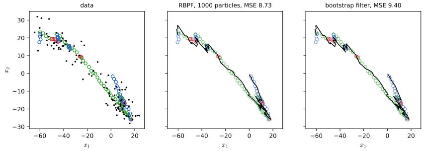
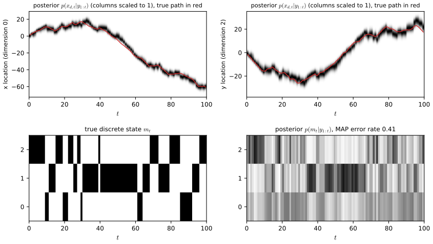
pp. 559–561 An object with state \(\bm z_t=(x_{1t},\dot x_{1t},x_{2t},\dot x_{2t})\) moves as \(\bm z_t=\bm F\bm z_{t-1}+\bm b_{m_t}+\mathcal N(\bm 0,0.2\bm I)\) (13.65) with \(\Delta=0.1\) and three regimes with biases \(\bm b_1=\bm 0\), \(\bm b_2=(-1.225,-0.35,1.225,0.35)\), \(\bm b_3=-\bm b_2\) (accelerate left, straight, accelerate right), the transition matrix \(\bm A\) with 0.8 on the diagonal and 0.1 elsewhere (13.67), \(\bm H=\bm I\) and \(\bm R=10\,\mathrm{diag}(2,1,2,1)\). Figure 13.6 compares the Rao-Blackwellised filter with the bootstrap filter (1000 particles each); Figure 13.7 shows the posterior in the mixture-of-Gaussians form, and the filtered probabilities of the regime. In my simulation the RBPF has position mean squared error 8.73 against 9.40 for the bootstrap filter, and misclassifies 41% of the regimes (the book reports 7.66 versus 10.95 and 29% on its run; the simulations differ). Averaged over six independent simulations with 300 particles the errors are 3.94 and 4.08: a modest gain in this noisy setting (these are averages over few runs, not a significance claim). Misclassifying an isolated regime hardly harms the position estimate, because the continuous state is integrated out given the regime history.
13.4.3 Example: FastSLAM
pp. 560–563 In simultaneous localisation and mapping a robot with pose \(\bm r_t\) estimates its own path and a map of \(K\) landmark locations \(\bm l^1,\dots,\bm l^K\) from distance measurements and controls \(\bm u_t\) (Figure 13.8 is the graphical model, Figure 13.9 a sketch of loop closing: the pose uncertainty grows while exploring and shrinks on returning to a known place, and the posterior precision matrix of (pose, landmarks) becomes dense, so a Kalman filter on the joint state costs \(O(K^3)\) per step). The RBPF idea: given the robot's path \(\bm r_{1:t}\), the landmarks are independent, \[ p(\bm l^{1:K}\given\bm r_{1:t},\bm y_{1:t})=\prod_{k=1}^Kp(\bm l^k\given\bm r_{1:t},\bm y_{1:t}). \] Indeed, for static landmarks with independent priors the posterior is proportional to \(\prod_kp(\bm l^k)\times\prod_\tau p(\bm y_\tau\given\bm r_\tau,\bm l^{k_\tau})\), where each observation involves one landmark \(k_\tau\), so it factorises over \(k\). Hence one samples paths \(\bm r_{1:t}\) with a particle filter and keeps one small (2-d) Kalman filter per landmark in each particle: cost \(O(NK)\) per step with a small \(N\), essentially linear in the number of landmarks (FastSLAM, Thrun et al. 2004; the occupancy-grid version with HMM filters is Murphy 2000). Since the figures of this section are a graphical model and a sketch from a textbook, they are not computed here.
13.5 Extensions of the particle filter
p. 563 Several extensions are mentioned: resample-move (add one or more MCMC steps targeting \(\pi_t\) after resampling to restore diversity; Section 13.6.3 uses it), particle smoothing (offline inference; the path-degeneracy of Section 13.2.3.2 makes the naive smoother poor), particle belief propagation (combining particles with loopy belief propagation, Chapter 9, to infer in general graphical models), and SMC samplers for static models (Section 13.6).
13.6 SMC samplers
pp. 563–564 An SMC sampler uses the particle filter to sample from a generic target \(\pi(\bm z)=\tilde\gamma(\bm z)/Z\) that is not a state-space model, as an alternative to MCMC. Its advantages: it estimates the normalising constant \(Z\); the transition kernel can be tuned adaptively from the current particles; and it parallelises easily. The recipe: define a sequence of distributions \(\pi_t(\bm z_t)\) on the same space, lift each to a distribution over the whole history, run particle filtering on the lifted sequence, and read off the final marginal.
13.6.1 Ingredients of an SMC sampler
pp. 564–565 One needs (i) distributions \(\pi_t(\bm z_t)=\tilde\gamma_t(\bm z_t)/Z_t\), \(t=0{:}T\), on one space; (ii) a forward kernel \(M_t(\bm z_t\given\bm z_{t-1})\) that proposes new samples; (iii) a backward kernel \(L_t(\bm z_t\given\bm z_{t+1})\) (a Markov kernel) that defines the lifted target \[ \pi_t(\bm z_{1:t})=\pi_t(\bm z_t)\prod_{s=1}^{t-1}L_s(\bm z_s\given\bm z_{s+1}), \tag{13.69} \] whose \(\bm z_t\)-marginal is \(\pi_t(\bm z_t)\). The incremental weight is \[ \alpha_t=\frac{\pi_t(\bm z_{1:t})}{\pi_{t-1}(\bm z_{1:t-1})M_t(\bm z_t\given\bm z_{t-1})}\propto\frac{\tilde\gamma_t(\bm z_t)}{\tilde\gamma_{t-1}(\bm z_{t-1})}\frac{L_{t-1}(\bm z_{t-1}\given\bm z_t)}{M_t(\bm z_t\given\bm z_{t-1})}\tag{13.70} \] (the generic algorithm 13.3 applies). If \(M_t\) is an MCMC kernel that leaves \(\pi_t\) invariant and \(L_{t-1}\) is its time reversal, \[ \pi_t(\bm z_t)L_{t-1}(\bm z_{t-1}\given\bm z_t)=\pi_t(\bm z_{t-1})M_t(\bm z_t\given\bm z_{t-1}),\tag{13.71} \] the weight collapses to \(\alpha_t=\tilde\gamma_t(\bm z_{t-1})/\tilde\gamma_{t-1}(\bm z_{t-1})\) (13.72–13.74). For real-valued unconstrained parameters the kernel can be \(K\) steps of random-walk Metropolis with proposal covariance \(\delta^2\hat{\bm\Sigma}_{t-1}\), \(\hat{\bm\Sigma}\) the weighted empirical covariance of the particles, with the scale of Roberts, Gelman and Gilks (see gap 13.12 and the notes on the book); gradient-based kernels (HMC, NUTS) or, for binary spaces, the sampler of Schaefer and Chopin (2013) are used in higher dimensions.
Filling the gap 13.10: the lifted target, the reversal kernel and the incremental weight pp. 564–565, (13.69)–(13.74)
Derivation
Marginal of (13.69). Integrate \(\bm z_1\) first: \(\int L_1(\bm z_1\given\bm z_2)\,\d\bm z_1=1\) because \(L_1\) is a Markov kernel in its first argument; then \(\bm z_2\), and so on up to \(\bm z_{t-1}\). What remains is \(\pi_t(\bm z_t)\). So particles for the lifted target, restricted to their last coordinate, are samples from \(\pi_t\).
Weight (13.70). Use the weight recursion (13.18) with the proposal \(q_t=M_t\) and the unnormalised lifted targets \(\tilde\gamma_t(\bm z_{1:t})=\tilde\gamma_t(\bm z_t)\prod_{s<t}L_s(\bm z_s\given\bm z_{s+1})\). The factors \(L_s\), \(s\le t-2\), cancel between numerator and denominator, leaving \(\tilde\gamma_t(\bm z_t)L_{t-1}(\bm z_{t-1}\given\bm z_t)/(\tilde\gamma_{t-1}(\bm z_{t-1})M_t(\bm z_t\given\bm z_{t-1}))\).
Reversal kernel. Suppose \(\int\pi_t(\bm z_{t-1})M_t(\bm z_t\given\bm z_{t-1})\,\d\bm z_{t-1}=\pi_t(\bm z_t)\) (invariance). Define \(L_{t-1}\) by (13.71). It is a legitimate kernel: \(\int L_{t-1}(\bm z_{t-1}\given\bm z_t)\,\d\bm z_{t-1}=\pi_t(\bm z_t)^{-1}\int\pi_t(\bm z_{t-1})M_t(\bm z_t\given\bm z_{t-1})\,\d\bm z_{t-1}=1\), the integral being exactly the invariance statement. Then, with \(\tilde\gamma_t=Z_t\pi_t\), \[ \alpha_t=\frac{Z_t\pi_t(\bm z_t)L_{t-1}(\bm z_{t-1}\given\bm z_t)}{Z_{t-1}\pi_{t-1}(\bm z_{t-1})M_t(\bm z_t\given\bm z_{t-1})}=\frac{Z_t\pi_t(\bm z_{t-1})M_t}{Z_{t-1}\pi_{t-1}(\bm z_{t-1})M_t}=\frac{\tilde\gamma_t(\bm z_{t-1})}{\tilde\gamma_{t-1}(\bm z_{t-1})}.\tag{13.74} \] The weight depends on the old point \(\bm z_{t-1}\) only, so it can be computed before the move; the algorithm is: reweight by (13.74), resample, move with the \(\pi_t\)-invariant kernel. (If the kernel instead leaves \(\pi_{t-1}\) invariant, the same computation gives the weight \(\tilde\gamma_t(\bm z_t)/\tilde\gamma_{t-1}(\bm z_t)\) at the new point, the order used in Algorithm 13.5 of the book; both are valid.) A finite-state example with a Metropolis kernel confirmed numerically that (13.70) with (13.71) equals (13.74) for every transition of positive probability.
Evidence. The lifted targets and weights form an ordinary SISR run, so \(\hat Z_T=\prod_t\frac1N\sum_i\alpha_t^i\) is unbiased for \(Z_T/Z_0\) (gap 13.3). Without resampling the weights multiply to \(\prod_t\tilde\gamma_t(\bm z_{t-1})/\tilde\gamma_{t-1}(\bm z_{t-1})\), the weight of annealed importance sampling (Neal 2001), as the book says in Section 13.6.2.
13.6.2 Likelihood tempering (geometric path)
pp. 565–566 A standard sequence interpolates geometrically between an easy distribution \(\tilde\gamma_0\) and the target, \[ \tilde\gamma_t(\bm z)=\tilde\gamma_0(\bm z)^{1-\lambda_t}\tilde\gamma(\bm z)^{\lambda_t},\qquad0=\lambda_0<\lambda_1<\dots<\lambda_T=1. \tag{13.75} \] (Without resampling this is annealed importance sampling.) For a Bayesian posterior, \(\tilde\gamma_0=\) prior, \(\tilde\gamma=\) prior \(\times\) likelihood, so that \(\tilde\gamma_t(\bm\theta)=\pi_0(\bm\theta)\,p(\mathcal D\given\bm\theta)^{\lambda_t}\) and the incremental weight (13.74) is \(p(\mathcal D\given\bm\theta)^{\delta_t}=\exp(-\delta_tE(\bm\theta))\), \(\delta_t=\lambda_t-\lambda_{t-1}\), with \(E=-\log p(\mathcal D\given\bm\theta)\) the negative log likelihood (13.77). (In (13.76) the book writes \(E=-\log p(\mathcal D,\bm\theta)\); read literally that would count the prior twice, see the notes on the book; in the bimodal example below \(E\) is the likelihood factor.) The increments must be chosen so that successive distributions are close: adaptive tempering picks \(\delta_t\) so that the ESS of the new weights is a chosen fraction of \(N\), \[ \delta_t=\text{the }\delta\in(0,1-\lambda_{t-1}]\text{ with }\mathrm{ESS}_{\mathrm{LW}}(\{-\delta E(\bm\theta^n_t)\})=\mathrm{ESS}_{\min},\tag{13.78} \] (the book writes \(\operatorname{argmin}_\delta(\mathrm{ESS}_{\mathrm{LW}}-\mathrm{ESS}_{\min})\), which as printed has no interior minimum: the intended statement is that the ESS equals the target, or the absolute difference is minimised; if no \(\delta\) in the interval gives that ESS, take \(\delta=1-\lambda_{t-1}\)); typically \(\mathrm{ESS}_{\min}=0.5N\). In the Gaussian case the optimal schedule can be written down (gap 13.11). Algorithm 13.5: draw \(\bm\theta_0^n\sim\pi_0\); while \(\lambda_t<1\): choose \(\delta_t\) by (13.78), set \(\lambda_t=\lambda_{t-1}+\delta_t\) and \(\tilde w^n=e^{-\delta_tE(\bm\theta^n)}\), normalise; resample and move each particle with a kernel that leaves the new tempered target invariant. Demonstration: the tempering sampler run on the bimodal example (presets 1 and 2).
Filling the gap 13.11: tempering weights, a monotone ESS, and the optimal schedule for Gaussians pp. 565–566, (13.75)–(13.78)
Derivation
Weights. From (13.74), \(\alpha_t=\tilde\gamma_t(\bm\theta)/\tilde\gamma_{t-1}(\bm\theta)=p(\mathcal D\given\bm\theta)^{\lambda_t-\lambda_{t-1}}\). Under \(\pi_{\lambda}\propto\pi_0p^{\lambda}\) its expectation is \(Z(\lambda+\delta)/Z(\lambda)\), \(Z(\lambda)=\int\pi_0p^\lambda\): for the bimodal example at \(\lambda=0.3\), \(\delta=0.2\) this ratio computed by quadrature equals the expectation of \(e^{-\delta E}\) under \(\pi_{0.3}\) to \(10^{-9}\). The product of these expected weights over \(t\) telescopes to \(Z(1)/Z(0)\), the evidence.
The ESS decreases with \(\delta\). Let \(\Lambda(\delta)=\log\E_{\pi}[e^{-\delta E}]\), convex in \(\delta\) (log of a moment generating function). For weights \(e^{-\delta E}\) the limiting ESS fraction is \(\E[w]^2/\E[w^2]=\exp(2\Lambda(\delta)-\Lambda(2\delta))\) and the derivative of its logarithm is \(2\Lambda'(\delta)-2\Lambda'(2\delta)\le0\) since \(\Lambda'\) is nondecreasing. So the ESS is a nonincreasing function of \(\delta\): the root of (13.78), if it exists, is unique and bisection on \([0,1-\lambda_{t-1}]\) finds it (this is what the code does).
Gaussian case (the "one can show" of the text). Let the prior be \(\N(0,1/a_0)\) and the energy \(E(\theta)=\tfrac b2\theta^2\), so \(\pi_\lambda=\N(0,1/p_\lambda)\) with precision \(p_\lambda=a_0+\lambda b\). For \(w=e^{-\delta E}\) and \(\theta\sim\pi_\lambda\), by the Gaussian integral \(\E[w]=(1+x)^{-1/2}\) and \(\E[w^2]=(1+2x)^{-1/2}\) with \(x=\delta b/p_\lambda\), so the ESS fraction is \[ \rho(x)=\frac{\E[w]^2}{\E[w^2]}=\frac{\sqrt{1+2x}}{1+x}, \] which depends on the step only through \(x=\delta b/p_\lambda\). Holding the ESS fraction constant therefore means holding \(x=c\) constant: \(p_{\lambda_t}=p_{\lambda_{t-1}}+\delta_tb=(1+c)p_{\lambda_{t-1}}\), i.e. the precision of the tempered distribution grows geometrically and \[ \lambda_t=\frac{a_0}b\big[(1+c)^t-1\big]. \] This is the book's "\(\lambda_t=(1+\gamma)^{t+1}-1\)" up to the constant \(a_0/b\) and a shift of the index: increase \(\lambda\) slowly at first and then in larger and larger steps. The simulated ESS fraction of \(e^{-\delta E}\) for \(a_0=1,b=3,\lambda=0.2,\delta=0.15\) agreed with \(\rho(x)\) to 0.005 with \(4\times10^6\) draws. To keep \(\rho=0.5\) the precision may grow by a factor \(1+x\approx7.46\) per step (practice problem 13.2): the ESS fraction is a conservative guide, and the number of stages is a rapidly increasing function of it (2, 3, 3, 5, 8, 13 stages for 0.5, 0.7, 0.8, 0.9, 0.95, 0.98 in the bimodal example below).
13.6.2.1 Example: sampling from a 1d bimodal distribution
pp. 565–567 Take \(p(\theta)\propto\N(\theta\given0,1)\exp(-E(\theta))\), \(E(\theta)=c(\|\theta\|^2-1)^2\), \(c=5\) (13.79): two modes near \(\pm1\) where the energy is low, separated by a barrier of height \(c\) at the origin (Figure 13.10a). Tempered versions \(\propto\N(\theta\given0,1)e^{-\lambda E}\) (Figure 13.10b) start at the Gaussian prior (\(\lambda=0\)) and end at the target. The book states that multimodal targets can be provably hard for other methods, including HMC, and shows HMC and NUTS stuck at the starting mode \(\theta_0=1\) (Figure 13.11a,b), while tempered SMC with a (single-step) HMC kernel recovers both modes (Figure 13.11c) with the adaptive schedule of Figure 13.11d, and reports 8 steps.
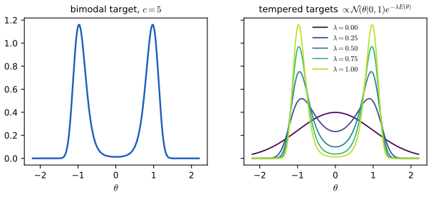
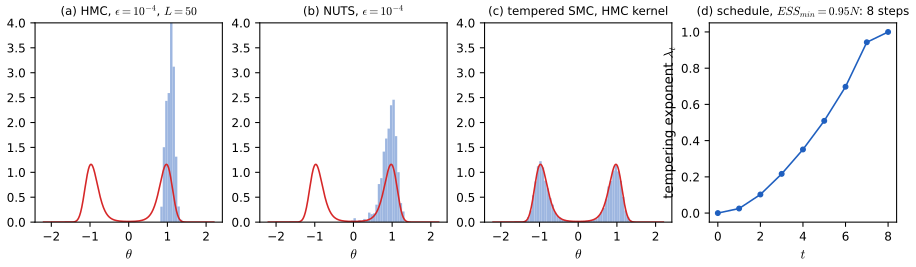
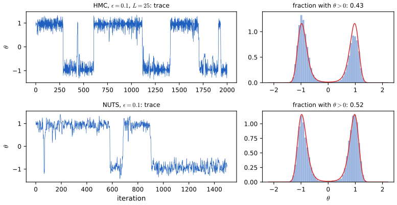
Three observations from the code, all confirmed numerically. (1) The estimate of the normalising constant is accurate: \(\hat Z=0.2115\) with 10000 particles against \(Z=0.21116\) by quadrature (an average over 20 runs with 4000 particles was within 0.3% of \(Z\), as unbiasedness predicts), and the mass on \(\theta>0\) is 0.49 (the target is symmetric). (2) The number of stages depends strongly on \(\mathrm{ESS}_{\min}\): with the stated \(0.5N\) the schedule has only 2 stages (\(\lambda=0,0.52,1\)); the 8 steps of the book's Figure 13.11d are obtained at \(0.95N\) (\(\lambda=0,0.025,0.103,0.216,0.351,0.509,0.698,0.943,1\), roughly geometric at first as predicted by gap 13.11), which is what the figure shows. (3) The failure of HMC and NUTS in Figures 13.11a,b is a property of the tiny step size \(\epsilon=10^{-4}\) used there: that setting moves a trajectory by only \(0.005\) per iteration, so in 10000 iterations the chain stays in \([0.82,1.36]\). The barrier is only \(c=5\) nats, and with a tuned step (\(\epsilon=0.1\), 25 leapfrog steps) HMC crosses it repeatedly, the fraction of time at \(\theta>0\) is 0.43 and \(\E[\theta^2]=0.883\) agrees with quadrature (0.882); NUTS with \(\epsilon=0.1\) does as well (own figure below). Hard multimodality for gradient samplers is real (barriers grow with \(c\) and with the dimension) but this example does not demonstrate it. In the demonstration a plain random-walk Metropolis chain from \(\theta=1\) also crosses at \(c=5\) in 5000 steps but not at \(c\ge10\) with a small step, while the SMC sampler keeps mass 1/2 on each mode throughout.
13.6.3 Data tempering
p. 567 For iid observations define \(\tilde\gamma_t(\bm\theta)=p(\bm\theta)p(\bm y_{1:t}\given\bm\theta)\) (13.80). The incremental weight (13.81) is the predictive density of the new observation given the old ones and \(\bm\theta\), \(p(\bm y_t\given\bm y_{1:t-1},\bm\theta)\). Each MCMC move needs the likelihood of all \(t\) data, so the cost is \(O(T^2)\) if one moves at every step; the iterated batch importance sampling (IBIS) algorithm of Chopin (2002) moves only when the ESS falls below a threshold and simply carries the particles over in between.
Filling the gap 13.12: the data-tempering weight, the evidence, the cost, and the random-walk scaling pp. 567–568, (13.80)–(13.81), Section 13.6.1
Derivation
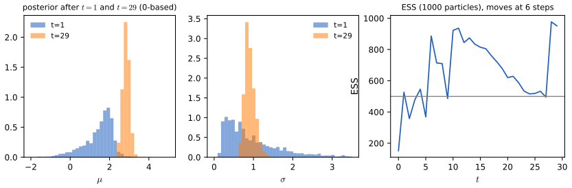
Weight and evidence. (13.74) gives \(\alpha_t(\bm\theta)=\dfrac{p(\bm\theta)p(\bm y_{1:t}\given\bm\theta)}{p(\bm\theta)p(\bm y_{1:t-1}\given\bm\theta)}=p(\bm y_t\given\bm y_{1:t-1},\bm\theta)\), which is \(p(\bm y_t\given\bm\theta)\) for conditionally independent data. The estimate \(\hat Z_T=\prod_t\frac1N\sum_i\alpha_t^i\) (with resampling resetting the weights) estimates \(Z_T=p(\bm y_{1:T})=\prod_tp(\bm y_t\given\bm y_{1:t-1})\), the marginal likelihood, and is unbiased (gap 13.3). For the Gaussian example of Figure 13.12 (30 observations, 1000 particles) it gave \(\log\hat Z=-46.51\) against \(-46.43\) by two-dimensional quadrature, and the weighted posterior means after 30 observations, 2.842 for \(\mu\) (grid: 2.843) and 0.910 for \(\sigma\) (grid: 0.910), agreed with the grid posterior.
Cost. A Metropolis acceptance ratio at stage \(t\) contains \(\prod_{s\le t}p(\bm y_s\given\bm\theta')\), \(t\) factors: moving at every step costs \(\sum_tt\propto T^2\); IBIS moves \(R\) times (here \(R=6\)) at cost \(\sum_{r}t_r\le RT\).
The random-walk scale. The book gives the proposal covariance as \(\delta^2\hat{\bm\Sigma}_{t-1}\) with \(\delta=2.38D^{-3/2}\). The classical result of Roberts, Gelman and Gilks (1997) is \(\delta=2.38/\sqrt D\), i.e. proposal covariance \((2.38^2/D)\hat{\bm\Sigma}\). Heuristic derivation for a target \(\N(\bm0,\bm I_D)\), proposal \(\bm y=\bm x+(\ell/\sqrt D)\bm\xi\): the log acceptance ratio is \(R=-\tfrac12(\|\bm y\|^2-\|\bm x\|^2)=-\tfrac{\ell}{\sqrt D}\bm x\cdot\bm\xi-\tfrac{\ell^2}{2D}\|\bm\xi\|^2\). Since \(\bm x\cdot\bm\xi\mid\bm x\sim\N(0,\|\bm x\|^2)\) with \(\|\bm x\|^2\approx D\) and \(\|\bm\xi\|^2\approx D\), \(R\approx\N(-\ell^2/2,\ell^2)\), and \(\E[\min(1,e^R)]=2\Phi(-\ell/2)\). The expected squared jump per step is \(\propto\ell^2\cdot2\Phi(-\ell/2)\), maximised at \(\ell\approx2.38\) with acceptance 0.234. In a 10-dimensional standard Gaussian, proposal sd \(2.38/\sqrt{10}\) gave acceptance 0.262, while \(2.38\cdot10^{-3/2}\) gave 0.908: the printed scale takes tiny steps that are almost always accepted. For \(D=1\) the two agree, which is probably why the typo is harmless in the one-dimensional example.
13.6.3.1 Example: IBIS for a 1d Gaussian
pp. 567–568 The data are 30 draws from \(\mathcal N(\mu=3.14,\sigma=1)\), the unknowns \(\bm\theta=(\mu,\sigma)\), the prior \(\N(\mu\given0,1)\operatorname{Ga}(\sigma\given a=1,b=1)\) and the kernel adaptive random-walk Metropolis. The text speaks of 20 particles with 50 moves each, "so we collect 1000 samples per time step", but the ESS plot has a threshold of 500 out of 1000: the effective population is 1000 particles, which is what is used here, with moves on the log scale of \(\sigma\) and five Metropolis steps per rejuvenation. The posterior concentrates near the true values (Figure 13.12a, after the prior's shrinkage of \(\mu\)), and the ESS (Figure 13.12b) falls below \(N/2\) only 6 times, so only 6 rejuvenation moves are needed in 30 steps.
13.6.4 Sampling rare events and extrema
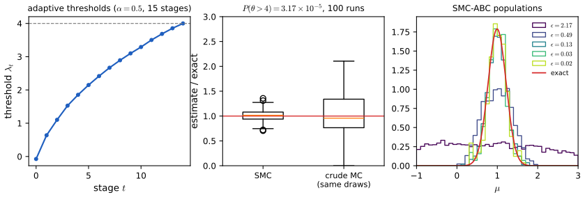
pp. 568–569 To sample \(\pi_0(\bm\theta)\) conditioned on the rare event \(S(\bm\theta)\ge\lambda^*\), use the sequence \[ \pi_t(\bm\theta)=\frac1{Z_t}\mathbb I(S(\bm\theta)\ge\lambda_t)\,\pi_0(\bm\theta),\qquad\lambda_0<\dots<\lambda_T=\lambda^*,\tag{13.82} \] a likelihood-tempering path with the indicator "likelihood" \(G_t=\mathbb I(S\ge\lambda_t)\) (13.83); \(Z_T=P_{\pi_0}(S\ge\lambda_T)\) (13.84) is also estimated. Thresholds can be set adaptively as the \(\alpha\)-quantile of the current scores, e.g. \(\alpha=0.5\) keeps the fittest half; this is the subset simulation of Cérou et al. (2012). It resembles the cross-entropy method of Section 6.7.5, which instead fits a parametric family to the survivors rather than moving them with a Markov kernel.
Filling the gap 13.13: the rare-event estimator as a product of conditional probabilities pp. 568–569, (13.82)–(13.84)
Derivation
Let \(A_t=\{S\ge\lambda_t\}\), a nested sequence \(A_0\supset A_1\supset\dots\supset A_T\) with \(A_0\) the whole space (\(\lambda_0=-\infty\)). Then \(P(A_T)=\prod_{t=1}^TP(A_t\given A_{t-1})\) (nestedness: \(P(A_t)=P(A_t\cap A_{t-1})=P(A_t\given A_{t-1})P(A_{t-1})\)), and \(P(A_t\given A_{t-1})=\E_{\pi_{t-1}}[G_t]\), \(G_t=\mathbb I_{A_t}\): the expected incremental weight of the SMC sampler, estimated by the fraction of the particles (distributed as \(\pi_{t-1}\)) that satisfy \(S\ge\lambda_t\). That is exactly (13.28), so \(\hat Z_T=\prod_t\hat p_t\) is unbiased (gap 13.3). With the quantile rule each factor is \(\alpha\), except the last, so \(T\approx\log P/\log\alpha\) stages. If the factors were estimated independently each from \(N\) independent particles, each has relative variance \((1-\alpha)/(\alpha N)\) and the product's relative variance is \(\approx T(1-\alpha)/(\alpha N)\). For \(P(\theta>4)=3.17\times10^{-5}\), \(\theta\sim\N(0,1)\), \(\alpha=0.5\), \(N=1000\) this is \(15/1000\), a relative standard deviation of 0.12; the simulation (100 runs, 15 stages, ten Metropolis moves per stage) gave 0.12 and a mean of 1.001 times the exact value (200 runs). Crude Monte Carlo with 165000 draws, about the work of the sampler, has relative standard deviation \(\sqrt{(1-P)/(MP)}=0.44\) (simulated 0.43): about four times larger, and the gap widens as \(P\to0\), since \(\log(1/P)\) grows much more slowly than \(1/P\). The kernel only needs to leave \(\pi_0\) restricted to \(A_t\) invariant; here random-walk Metropolis with the constraint \(\theta\ge\lambda_t\).
13.6.5 SMC-ABC and likelihood-free inference
p. 569 For a simulator \(\bm y\sim p(\cdot\given\bm\theta)\) whose likelihood cannot be evaluated, approximate Bayesian computation (ABC) accepts \((\bm\theta,\bm y)\) pairs with \(d(\bm y,\bm y^*)<\epsilon\) (or \(d(s(\bm y),s(\bm y^*))<\epsilon\) with a summary statistic \(s\)). SMC-ABC lowers the tolerance gradually, \(\epsilon_0>\epsilon_1>\dots\), using \[ \pi_t(\bm\theta,\bm y)=\frac1{Z_t}\pi_0(\bm\theta)p(\bm y\given\bm\theta)\mathbb I(d(\bm y,\bm y^*)<\epsilon_t),\tag{13.85} \] like the rare-event sampler but with the quality of \(\bm\theta\) judged in data space (Del Moral et al. 2012). It is popular in genetics and epidemiology but slow and not scalable to high dimension; there one trains a generative model (e.g. a flow) of the simulator and then does ordinary inference (the book's Chapter 26 and Section 26.1 on implicit models).
Filling the gap 13.14: what the ABC target is and why it converges to the posterior as \(\epsilon\to0\) p. 569, (13.85)
Derivation
Marginal over the simulated data. Integrating (13.85) over \(\bm y\), \(\pi_\epsilon(\bm\theta)\propto\pi_0(\bm\theta)\,P_{\bm y\sim p(\cdot\given\bm\theta)}(d(\bm y,\bm y^*)<\epsilon)\): the prior times the chance that the simulator reproduces the data to accuracy \(\epsilon\).
Limit. For continuous data with a continuous bounded likelihood \(p(\bm y\given\bm\theta)\), \(P(d<\epsilon\given\bm\theta)/\mathrm{vol}(B_\epsilon)\to p(\bm y^*\given\bm\theta)\) as \(\epsilon\to0\) (the average of a continuous function over a shrinking ball), so by dominated convergence \(\pi_\epsilon\to p(\bm\theta\given\bm y^*)\). With a summary statistic the limit is \(p(\bm\theta\given s(\bm y^*))\), equal to the true posterior if \(s\) is sufficient.
Example. \(y_i\sim\N(\mu,1)\), \(i\le n\), prior \(\N(0,3^2)\), \(s=\bar y\) (sufficient), \(s\given\mu\sim\N(\mu,1/n)\). With \(d=|s-s^*|\), \(P(d<\epsilon\given\mu)=\Phi((s^*+\epsilon-\mu)\sqrt n)-\Phi((s^*-\epsilon-\mu)\sqrt n)\), so \(\pi_\epsilon\) is explicit. For \(n=20\), \(s^*=1\) the \(L^1\) distance from the exact posterior (mean \(0.9945\), sd 0.223) is 1.06, 0.53, 0.031 and 0.0003 for \(\epsilon=1,0.5,0.1,0.01\). The SMC-ABC run (3000 particles, \(\alpha=0.5\), three moves per stage) ended at \(\epsilon=0.02\) with mean 0.995 and sd 0.232 (own figure below); the moves are random-walk Metropolis proposals of \(\bm\theta'\) together with a fresh simulation \(\bm y'\), accepted if \(d(\bm y',\bm y^*)<\epsilon_t\) and with the prior ratio, a pseudo-marginal move that leaves (13.85) invariant (gap 13.18). In a 4000-particle check the final population's sd was within 7% of that of the \(\epsilon\)-ABC posterior (slight under-dispersion from finite resampling).
13.6.6 SMC2
p. 569 The SMC sampler needs the ratio \(\tilde\gamma_t(\bm\theta)/\tilde\gamma_{t-1}(\bm\theta)\), which for a latent-variable model is a likelihood that cannot be evaluated. SMC2 replaces it by the unbiased particle-filter estimate \(\hat Z_t/\hat Z_{t-1}\) (13.10): an outer SMC over parameters, each parameter particle carrying an inner particle filter over the latent states (Chopin, Jacob and Papaspiliopoulos 2013). It is valid for the same reason as particle MCMC: the estimate is unbiased, so the extended target with the filter's internal randomness has the right marginal (gap 13.18).
13.6.7 Variational filtering SMC
pp. 569–570 A proposal \(q_\phi\) (e.g. a neural network) can be learned by maximising a lower bound on the log evidence given by SMC. With the particle approximation \(\hat\pi_T(\bm z_{1:T};\phi,\theta)\) of \(\pi_T(\bm z_{1:T};\theta)\) and the unbiased evidence estimate \(\hat Z_T\), \[ 0\le\KL\big(\E[\hat\pi_T(\bm z_{1:T})]\,\|\,\pi_T(\bm z_{1:T})\big)\le-\E\Big[\log\frac{\hat Z_T}{Z_T}\Big],\tag{13.86} \] \[ \E[\log\hat Z_T(\theta,\phi)]\le\log\E[\hat Z_T]=\log Z_T(\theta).\tag{13.87, 13.88} \] So \(\E\log\hat Z_T\) is a lower bound (the FIVO, variational SMC and auto-encoding SMC objectives) that can be maximised over \(\theta\) and \(\phi\) by stochastic gradients; the resampling step is not differentiable, and in practice one ignores the dependence of the resampling on the parameters or uses differentiable relaxations.
Filling the gap 13.15: the SMC lower bound and the KL bound pp. 569–570, (13.86)–(13.88)
Derivation
(13.88) is Jensen's inequality applied to the concave logarithm, together with \(\E[\hat Z_T]=Z_T\) (gap 13.3). For (13.86) work on the extended space of the whole SMC run (Andrieu, Doucet and Holenstein 2010), for SISR with multinomial resampling at every step.
Joint law of a run. A run consists of the particles \(\bm x=(x_t^i)\) and the ancestor indices \(\bm a=(a^i_{t-1})\), with density \[ \psi(\bm x,\bm a)=\prod_{i=1}^Nq_1(x_1^i)\prod_{t=2}^T\prod_{i=1}^NW_{t-1}^{a_{t-1}^i}\,q_t\big(x_t^i\given x^{a_{t-1}^i}_{1:t-1}\big),\qquad W_t^j=\frac{\alpha_t^j}{\sum_k\alpha_t^k}. \] Choose a final index \(k\) with probability \(W_T^k\) and write \(\bm b=(b_1,\dots,b_T=k)\) for its lineage (\(b_{t-1}=a_{t-1}^{b_t}\)). Let \(\tilde q(\bm x,\bm a,k)=\psi(\bm x,\bm a)W_T^k\). Its marginal on the selected path \(x^{\bm b}_{1:T}\) is by construction \(\E[\hat\pi_T]\).
The tilted law. Put \(\tilde\pi(\bm x,\bm a,k)=\tilde q(\bm x,\bm a,k)\,\hat Z_T/Z_T\). It is nonnegative and integrates to \(\E[\hat Z_T]/Z_T=1\) (using \(\sum_kW_T^k=1\) and gap 13.3). Its marginal on the selected path is \(\pi_T\): expand \(\hat Z_TW_T^k=\prod_{t<T}\big(\frac1N\sum_j\alpha_t^j\big)\frac1N\alpha_T^k\), and let \(\psi_{\bm b}=q_1(x_1^{b_1})\prod_{t\ge2}W_{t-1}^{b_{t-1}}q_t(x_t^{b_t}\given x^{b_{t-1}}_{1:t-1})\) be the factors of \(\psi\) belonging to the lineage. Using \(W_{t}^{b_t}=\alpha_t^{b_t}/\sum_j\alpha^j_t\) and \(\tilde w_T=\prod_t\alpha_t=\tilde\gamma_T/q_T\) (13.17), \[ \psi_{\bm b}\cdot\prod_{t<T}\sum_j\alpha_t^j\cdot\alpha_T^{k}=q_1\prod_tq_t\prod_t\alpha_t^{b_t}=\tilde\gamma_T(x^{\bm b}_{1:T}),\quad\text{so}\quad\tilde\pi=\frac1{N^T}\,\pi_T(x^{\bm b}_{1:T})\,\frac{\psi(\bm x,\bm a)}{\psi_{\bm b}}. \] The ratio \(\psi/\psi_{\bm b}\) is the conditional density of all the other particles and indices given the lineage, so it integrates to 1. Summing over the \(N^T\) possible lineages (all index vectors \(\bm b\)), each contributing \(N^{-T}\pi_T(x^{\bm b})\), the marginal on the selected path is \(\pi_T\).
The bound. \(\KL(\tilde q\|\tilde\pi)=\E_{\tilde q}\log(\tilde q/\tilde\pi)=-\E\log(\hat Z_T/Z_T)\). Marginalising two distributions onto a function of the variables can only decrease their KL divergence (the chain rule of KL, \(\KL\ge0\) for the conditionals), so \(\KL(\E[\hat\pi_T]\|\pi_T)\le\KL(\tilde q\|\tilde\pi)\), which is (13.86). Both inequalities were checked on a two-state hidden Markov model with three observations (all paths enumerable; the distribution of the selected path from 300000 runs): with \(N=2\), \(\KL=0.404\le0.776=-\E\log(\hat Z/Z)\); with \(N=10\), \(0.0138\le0.136\). The gap in (13.88) shrinks as \(N\) grows, as the second numbers show.
13.6.8 Variational smoothing SMC
pp. 570–571 Filtering SMC has targets \(\pi_t(\bm z_{1:t})=p_\theta(\bm z_{1:t}\given\bm y_{1:t})\) that ignore future data, which hurts when fitting offline sequences: particles that fit the past can make the future unlikely, producing impoverishment and a high-variance bound. SIXO (smoothing inference with twisted objectives, Lawson et al. 2022) targets the smoothing distributions \(\pi_t(\bm z_{1:t})=p_\theta(\bm z_{1:t}\given\bm y_{1:T})\) through twisted particle filters: write \[ p_\theta(\bm z_{1:t},\bm y_{1:T})=p_\theta(\bm z_{1:t},\bm y_{1:t})\,p_\theta(\bm y_{t+1:T}\given\bm z_t)\approx p_\theta(\bm z_{1:t},\bm y_{1:t})\,r_\psi(\bm y_{t+1:T},\bm z_t),\tag{13.89–13.91} \] with a learned twisting function \(r_\psi\) ("lookahead"). The density-ratio identity \[ p_\theta(\bm y_{t+1:T}\given\bm z_t)=\frac{p_\theta(\bm z_t\given\bm y_{t+1:T})\,p_\theta(\bm y_{t+1:T})}{p_\theta(\bm z_t)}\propto\frac{p_1}{p_2},\qquad p_1=p_\theta(\bm z_t,\bm y_{t+1:T}),\;p_2=p_\theta(\bm z_t)p_\theta(\bm y_{t+1:T}),\tag{13.92} \] reduces the learning of \(r_\psi\) to binary classification between pairs \((\bm z_t,\bm y_{t+1:T})\) from one simulated sequence (positives) and pairs whose \(\bm z_t\) and \(\bm y_{t+1:T}\) come from independent sequences (negatives), as in the density-ratio method of Section 2.7.5 (the book's Section 2.7.5 in these notes). The method optimises the bound \(\mathcal L_{\mathrm{SIXO}}=\E\log\hat Z_{\mathrm{SIXO}}\le\log\E\hat Z_{\mathrm{SIXO}}=\log p_\theta(\bm y_{1:T})\) (13.93, 13.94) over \(\theta,\phi,\psi\) in a variational-EM fashion. Lawson et al. prove that if the optimal proposal and lookahead lie in the model classes and the optimum is unique, the bound is tight at the optimum for every number of particles \(N_s\ge1\), unlike FIVO.
Filling the gap 13.16: why exact twisting and the optimal proposal give a zero-variance evidence estimate pp. 570–571, (13.89)–(13.94)
Derivation
Factorisation (13.90). In a state-space model \(p(\bm y_{t+1:T}\given\bm z_{1:t},\bm y_{1:t})=p(\bm y_{t+1:T}\given\bm z_t)\), because given \(\bm z_t\) the future observations are independent of the earlier states and observations (d-separation). Hence \(p(\bm z_{1:t},\bm y_{1:T})=p(\bm z_{1:t},\bm y_{1:t})\beta_t(\bm z_t)\) with the backward message \(\beta_t(\bm z_t)=p(\bm y_{t+1:T}\given\bm z_t)\) (\(\beta_T\equiv1\)).
Density ratio (13.92). Bayes' rule gives the first equality; \(p(\bm y_{t+1:T})\) does not depend on \(\bm z_t\), so \(\beta_t(\bm z_t)\propto p_1/p_2\) and the constant cancels when the weights are normalised. With equal class priors a Bayes-optimal classifier of "positive" against "negative" is \(D^*=p_1/(p_1+p_2)\), whence \(D^*/(1-D^*)=p_1/p_2\); a classifier trained with the logistic loss approximates \(D^*\), so \(r_\psi=D_\psi/(1-D_\psi)\).
Zero variance. Take the targets \(\tilde\gamma_t(\bm z_{1:t})=p(\bm z_{1:t},\bm y_{1:t})\beta_t(\bm z_t)=p(\bm z_{1:t},\bm y_{1:T})\) and the proposals \(q_t(\bm z_t\given\bm z_{1:t-1})=p(\bm z_t\given\bm z_{1:t-1},\bm y_{1:T})\), which are the locally optimal proposals of gap 13.7 for these targets. Then for \(t\ge2\) \[ \alpha_t=\frac{p(\bm z_{1:t},\bm y_{1:T})}{p(\bm z_{1:t-1},\bm y_{1:T})\,p(\bm z_t\given\bm z_{1:t-1},\bm y_{1:T})}=1, \] because \(p(\bm z_{1:t},\bm y_{1:T})=p(\bm z_t\given\bm z_{1:t-1},\bm y_{1:T})p(\bm z_{1:t-1},\bm y_{1:T})\), and \(\alpha_1=\int p(\bm z_1,\bm y_{1:T})\,\d\bm z_1=p(\bm y_{1:T})\) (the normaliser of the first optimal proposal). Every weight is the same constant, so \(\hat Z=p(\bm y_{1:T})\) exactly, with zero variance and for any \(N_s\ge1\); the bound (13.94) is tight. I checked the algebra for a linear-Gaussian model by computing \(\beta_t\) in closed form (a Gaussian exponent obtained by backward recursion): the integral \(\int p(z_1)p(y_1\given z_1)\beta_1(z_1)\,\d z_1\) reproduced the Kalman log-evidence to \(10^{-6}\), and the normaliser \(\int p(z_t\given z_{t-1})p(y_t\given z_t)\beta_t(z_t)\,\d z_t\) equalled \(\beta_{t-1}(z_{t-1})\) to \(10^{-6}\), which is \(\alpha_t=1\). With an imperfect twist the weights vary and the bound is looser; learning \(\psi\) pushes the weights toward this ideal.
S13.2 Particle MCMC methods (supplement)
Supp. pp. 152–155 The unbiased evidence estimate \(\hat Z(\bm u)\) of SMC, a function of the random numbers \(\bm u\) the algorithm consumes (those that generate the states, \(\bm u_{z}\), and those that choose ancestors, \(\bm u_a\); \(\bm u\sim\tau(\bm u)\), representable by a random seed), \[ \hat Z_t(\bm u)=\prod_{s=1}^t\frac1{N_s}\sum_{n=1}^{N_s}\tilde w_s^n(\bm u),\qquad\E_{\tau}[\hat Z_t(\bm u)]=Z_t,\tag{S13.1, S13.2} \] can be plugged into MCMC algorithms for models with intractable likelihood: pseudo-marginal methods (Andrieu and Roberts 2009), the basis of many probabilistic programming systems. (The supplement numbers equations and algorithms 13.1, 13.2, ... independently of the main text; they are prefixed S here.)
S13.2.1 Particle marginal Metropolis–Hastings (PMMH)
Supp. pp. 153–154 For \(p(\bm\theta\given\bm y)\propto p(\bm\theta)p(\bm y\given\bm\theta)\) with \(p(\bm y\given\bm\theta)=\int p(\bm y,\bm h\given\bm\theta)\,\d\bm h\) intractable, the Metropolis–Hastings acceptance ratio (S13.3) cannot be evaluated; replace the likelihood by \(\hat Z(\bm u',\bm\theta')\), a particle-filter estimate, and apply MH on the extended space of \((\bm\theta,\bm u)\): \[ A=\min\Big\{1,\frac{\hat Z(\bm u',\bm\theta')\,p(\bm\theta')\,q(\bm\theta_{j-1}\given\bm\theta')}{\hat Z(\bm u_{j-1},\bm\theta_{j-1})\,p(\bm\theta_{j-1})\,q(\bm\theta'\given\bm\theta_{j-1})}\Big\}.\tag{S13.4} \] A latent trajectory \(\bm h'\) is drawn from the particle approximation \(\hat p(\bm h\given\bm\theta,\bm y,\bm u)=\sum_iW_T^i\delta(\bm h_{1:T}-\bm h_{1:T}^i)\) and accepted or rejected together with \(\bm\theta'\). Algorithm S13.1 (PMMH): for \(j=1{:}J\): propose \(\bm\theta'\sim q(\cdot\given\bm\theta_{j-1})\), \(\bm u'\sim\tau\), run SMC to get \(\hat Z(\bm u',\bm\theta')\) and \(\bm h'\); accept with probability (S13.4), in which case \((\bm\theta_j,\bm u_j,\bm h_j)=(\bm\theta',\bm u',\bm h')\), otherwise keep the old triple.
S13.2.2 Particle independent Metropolis–Hastings (PIMH)
Supp. pp. 153–154 With \(\bm\theta\) fixed and only the latent states of interest, the latent draw is independent of the chain's current state, hence an independence sampler on \(\bm u\) with acceptance \(\min(1,\hat Z(\bm u')/\hat Z(\bm u_{j-1}))\) (Algorithm S13.2). Its advantage over plain SMC is that it can return unbiased estimates of smoothing expectations \(\int\varphi(\bm h_{1:T})\pi(\bm h_{1:T}\given\bm\theta,\bm y)\,\d\bm h\) (Middleton et al. 2019), whereas direct SMC is only consistent for them (it is unbiased for \(Z\) alone).
S13.2.3 Particle Gibbs
Supp. pp. 154–155 Instead of proposing, update \((\bm\theta,\bm h)\) by Gibbs sampling: given the current \(\bm h^{(j-1)}\), run a conditional SMC with \(N-1\) fresh trajectories and the retained one as the \(N\)th particle, pick a new \(\bm h^{(j)}\) from the weighted final population, then draw \(\bm\theta^{(j)}\sim p(\bm\theta\given\bm h^{(j)},\bm y)\). No proposal needs to be specified; ancestor sampling (Lindsten, Jordan and Schön 2014) improves mixing in state-space models.
Filling the gap 13.18: why PMMH, PIMH and particle Gibbs have the exact posterior as invariant law Supp. pp. 152–155
Derivation
Pseudo-marginal principle. Define on \((\bm\theta,\bm u)\) the density \(\bar\pi(\bm\theta,\bm u)\propto p(\bm\theta)\,\hat Z(\bm u,\bm\theta)\,\tau(\bm u)\). Since \(\hat Z\ge0\) and, by unbiasedness (gap 13.3), \(\int\hat Z(\bm u,\bm\theta)\tau(\bm u)\,\d\bm u=p(\bm y\given\bm\theta)\), the \(\bm\theta\)-marginal is \(\propto p(\bm\theta)p(\bm y\given\bm\theta)\), the posterior, whatever \(N\) is. Run Metropolis–Hastings on \(\bar\pi\) with the proposal \(q(\bm\theta'\given\bm\theta)\tau(\bm u')\) (a fresh set of random numbers). The acceptance ratio is \[ \frac{p(\bm\theta')\hat Z(\bm u',\bm\theta')\tau(\bm u')}{p(\bm\theta)\hat Z(\bm u,\bm\theta)\tau(\bm u)}\cdot\frac{q(\bm\theta\given\bm\theta')\tau(\bm u)}{q(\bm\theta'\given\bm\theta)\tau(\bm u')}=\frac{\hat Z(\bm u',\bm\theta')p(\bm\theta')q(\bm\theta\given\bm\theta')}{\hat Z(\bm u,\bm\theta)p(\bm\theta)q(\bm\theta'\given\bm\theta)}, \] the \(\tau\) factors cancelling: this is (S13.4). A standard MH chain on \(\bar\pi\) is reversible with respect to \(\bar\pi\), so its \(\bm\theta\)-marginal is the posterior. The estimate is noisy but never wrong: noise only lowers the acceptance rate and makes the chain stick, since a lucky large \(\hat Z\) is hard to leave. Numerically: on an AR(1)-plus-noise model, 4000 bootstrap-filter likelihood estimates with 50 particles at \(\phi=0.7\) had mean \(1.00\pm0.01\) times the Kalman likelihood, and PMMH with only 30 particles reproduced the exact posterior mean and sd of \(\phi\) (the chain of 6000 steps: mean within 0.04, sd within 20%), while the figure shows how the chain sticks for \(N=10\) (acceptance 0.15 against 0.59 for \(N=100\)). A rule of thumb from the literature is to choose \(N\) so that \(\mathrm{sd}(\log\hat Z)\approx1\)–\(1.5\) (here 0.63 at \(N=100\), 2.4 at \(N=10\)).
With the latent path. Extend the state by the run's ancestry and the selected index \(k\) as in gap 13.15, with target \(\tilde\pi_{\bm\theta}(\bm x,\bm a,k)=\psi_{\bm\theta}(\bm x,\bm a)W_T^k\hat Z/Z(\bm\theta)\), whose marginal on the selected path is \(p(\bm h_{1:T}\given\bm\theta,\bm y)\); then \(\bar\pi(\bm\theta,\bm x,\bm a,k)\propto p(\bm\theta)Z(\bm\theta)\tilde\pi_{\bm\theta}=p(\bm\theta)\hat Z\,\psi W^k\) has marginal \(p(\bm\theta,\bm h\given\bm y)\) on \((\bm\theta,\bm h)\), and the same MH argument gives Algorithm S13.1 with the acceptance ratio (S13.4) (the factor \(W_T^k\) is part of the proposal and cancels).
PIMH. Fix \(\bm\theta\). The target is \(\tilde\pi\propto\tilde q\,\hat Z\) with \(\tilde q=\psi W_T^k\) (gap 13.15) and the proposal is an independent draw from \(\tilde q\). The independence-sampler ratio is \(\frac{\tilde\pi(\bm w')\tilde q(\bm w)}{\tilde\pi(\bm w)\tilde q(\bm w')}=\hat Z'/\hat Z\), the acceptance probability of Algorithm S13.2. In a test with 15 observations of the AR(1) model, 6000 PIMH iterations with 50 particles had a chain mean of \(z_T\) within 0.08 of the exact Kalman filtering mean.
Particle Gibbs. By gap 13.15 the target \(\tilde\pi(\bm x,\bm a,k)=N^{-T}\pi_T(x^{\bm b})\,\psi(\bm x,\bm a)/\psi_{\bm b}\) is a joint density in which, given the lineage \(\bm b\) and its values \(x^{\bm b}\), the other particles and ancestor indices have the conditional density \(\psi(\cdot\given\bm b,x^{\bm b})\): exactly what conditional SMC samples (run SMC with the retained path fixed as particle \(N\) and the \(N-1\) others generated normally). Conversely, given all particles and ancestors, \(\tilde\pi(k\given\bm x,\bm a)\propto W_T^k\), so choosing the new path with probability \(W^k_T\) is the exact conditional of the index. Both steps are exact Gibbs updates of \(\tilde\pi\), so \(\tilde\pi\) is invariant, hence so is its marginal \(\pi_T\) on the path; the parameter step is an ordinary Gibbs draw. (Ergodicity, i.e. that the chain mixes, needs the usual conditions, in particular \(N\ge2\); the proof above only concerns invariance.)
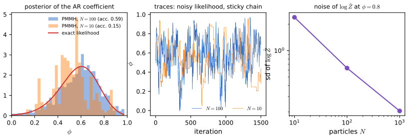
Practice problems
The book has no exercises for this chapter. These three short problems are my own; each was solved with the code and checked numerically.
Practice problem 13.1 (evidence of one importance-sampling step). Let \(z\sim\N(0,1)\), \(y\mid z\sim\N(z,1)\), and \(\hat Z=\frac1N\sum_i\N(y\given z_i,1)\) with \(z_i\) iid from the prior (one bootstrap step). Show that \(\hat Z\) is unbiased for \(p(y)=\N(y\given0,2)\) and find \(\var\hat Z\). Evaluate the relative standard deviation for \(y=0.8\), \(N=50\).
Solution
\(\E\hat Z=\int\N(y\given z,1)\N(z\given0,1)\,\d z=\N(y\given0,2)\) (a convolution of Gaussians, gap 13.3 for \(t=1\)). For the second moment use \(\N(y\given z,1)^2=\frac1{2\pi}e^{-(y-z)^2}=\frac1{2\sqrt\pi}\N(z\given y,\tfrac12)\), so \(\E[\N(y\given z,1)^2]=\frac1{2\sqrt\pi}\int\N(z\given y,\tfrac12)\N(z\given0,1)\,\d z=\frac{\N(y\given0,3/2)}{2\sqrt\pi}\). Hence \[ \var\hat Z=\frac1N\Big[\frac{\N(y\given0,3/2)}{2\sqrt\pi}-\N(y\given0,2)^2\Big]. \] For \(y=0.8\): \(\N(0.8\given0,2)=0.2404\), the bracket is \(0.07424-0.05778=0.01646\), \(\var\hat Z=3.29\times10^{-4}\) and the relative standard deviation is \(\sqrt{3.29\times10^{-4}}/0.2404=0.075\). A simulation with \(2\times10^5\) replications gave a mean of 1.000 times \(p(y)\) and a variance matching to 3%.
Practice problem 13.2 (one tempering step). The prior is \(\N(0,1/a_0)\) and \(p(\mathcal D\given\theta)^{\lambda}=e^{-\lambda b\theta^2/2}\). In the large-\(N\) limit, by what factor can the precision \(p_\lambda=a_0+\lambda b\) of the tempered distribution grow in one step while the ESS of the incremental weights stays at least half of \(N\)?
Solution
From gap 13.11 the ESS fraction for a step \(\delta\) is \(\rho(x)=\sqrt{1+2x}/(1+x)\), \(x=\delta b/p_\lambda\), which decreases from 1 at \(x=0\) to 0. Solve \(\rho(x)=\tfrac12\): squaring, \(4(1+2x)=(1+x)^2\), i.e. \(x^2-6x-3=0\), \(x=3+\sqrt{12}=6.464\). The new precision is \(p_\lambda+\delta b=(1+x)p_\lambda=7.46\,p_\lambda\): the standard deviation of the tempered target shrinks by a factor \(\sqrt{7.46}=2.73\) in one step. With the conservative fraction 0.95 one gets \(\rho=0.95\Rightarrow x\approx0.45\) and a growth factor of only 1.45 per step, which explains the 8 steps needed at \(0.95N\).
Practice problem 13.3 (systematic resampling by hand). With \(N=4\) and \(W=(0.1,0.2,0.3,0.4)\) list the possible offspring vectors of systematic resampling with their probabilities, and the variance of the offspring count of each particle. Compare with multinomial resampling.
Solution
The cumulative weights are \(0.1,0.3,0.6,1\), the points \(U_i=(i-1+u)/4\), \(u\sim\mathrm{Unif}(0,1)\). Tracking which interval each point falls in as \(u\) increases gives three outcomes: for \(u\in[0,0.2)\) the offspring vector is \((1,1,1,1)\); for \(u\in[0.2,0.4)\) it is \((1,0,2,1)\); for \(u\in[0.4,1)\) it is \((0,1,1,2)\), with probabilities \(0.2,0.2,0.6\). (The breakpoints are the values of \(u\) at which some point crosses a cumulative weight, e.g. \(U_1=u/4=0.1\) at \(u=0.4\), \(U_2=(1+u)/4=0.3\) at \(u=0.2\).) Check: \(\E O=(0.4,0.8,1.2,1.6)=NW\). Particle 1 has one child with probability 0.4, so variance \(0.4\cdot0.6=0.24\); the variances are \((0.24,0.16,0.16,0.24)=\mathrm{frac}(NW)(1-\mathrm{frac}(NW))\), total 0.8. For multinomial the variances are \(NW(1-W)=(0.36,0.64,0.84,0.96)\), total 2.8, three and a half times larger. A fine grid over \(u\) reproduced the table.
Demonstrations
| Page | What it shows | In the notes |
|---|---|---|
| The bootstrap particle filter | A bootstrap filter on a linear-Gaussian model (exact Kalman filter and exact log evidence shown) and on the 2-d spiral of Figure 13.1: number of particles, resampling scheme and threshold, state and observation noise; ESS over time, weight and path degeneracy, evidence estimate and its spread over 20 seeds. Presets: 1 baseline; 2 no resampling (SIS); 3 few particles; 4 precise sensor; 5 adaptive resampling; 6 multinomial resampling; 7 the spiral. | 13.2.2, 13.2.3, 13.2.5 |
| SMC with adaptive tempering | The bimodal target of (13.79): tempered densities and particles stage by stage, the ESS-driven schedule, the evidence estimate against the exact value, the mode balance, and a random-walk Metropolis chain for contrast. Presets: 1 the book's setting; 2 conservative schedule (8 stages); 3 higher barrier; 4 no moves; 5 few particles; 6 large-step baseline. | 13.6.2, 13.6.2.1 |
| Resampling schemes | The inverse-cdf staircase and ancestors of one draw, the offspring counts, and exact against simulated offspring variance for multinomial, stratified and systematic resampling, with the probability of losing a particle and the spread of the resampled estimate. Presets: 1 equal weights; 2 moderate spread; 3 very uneven weights; 4 large \(N\); 5 five particles. | 13.2.4 |
The Python code that produces every figure of this page is code/ch13_sequential_monte_carlo.py (see the code index); the data of the spiral demonstration are data/ch13-spiral.json. Companion demos: importance sampling in the Bishop course.
Notes on the book
Points where the book is imprecise
- (13.2) and (13.3), double counting. The joint is written \(p(\bm z_1)p(\bm y_1\given\bm z_1)\prod_{t=1}^Tp(\bm z_t\given\bm z_{t-1})p(\bm y_t\given\bm z_t)\), and (13.3) has \(\prod_{s=1}^t\); starting the product at 1 repeats the first observation factor (and needs a \(\bm z_0\)). It should start at \(t=2\), as in (13.5).
- Section 13.1.3, temperatures. "\(0=\tau_t<\dots<\tau_T=1\)" should read \(\tau_1\) for the first value.
- Algorithm 13.3, line 8. The test is on \(\mathrm{ESS}(\tilde w^{1:N_s}_{t-1})\), the old weights; the resampling that follows is of \(\tilde w_t\), so the test should use the weights of step \(t\) that were just computed (otherwise the decision lags one step).
- (13.76), (13.77), meaning of \(E\). The text defines the energy as \(E(\bm\theta)=-\log p(\mathcal D,\bm\theta)\). The path \(\pi_0^{1-\lambda}(\pi_0p)^\lambda=\pi_0\,p^\lambda\) is the right one, but its incremental weight is \(p(\mathcal D\given\bm\theta)^{\delta}\), which equals \(e^{-\delta E}\) only if \(E\) is the negative log likelihood (as in the bimodal example, where the prior is the Gaussian and \(E\) the likelihood factor). With \(E=-\log p(\mathcal D,\bm\theta)\) the weight would be \((\pi_0p)^\delta\), counting the prior again.
- (13.78). \(\operatorname{argmin}_\delta(\mathrm{ESS}_{\mathrm{LW}}(\delta)-\mathrm{ESS}_{\min})\) as printed is minimised at the end of the interval because the difference is monotone in \(\delta\); the intended definition is the root of \(\mathrm{ESS}_{\mathrm{LW}}(\delta)=\mathrm{ESS}_{\min}\) (or the minimiser of the absolute difference), as in the code of the notes.
- Section 13.6.1, the scaling \(\delta=2.38D^{-3/2}\). The optimal scale for random-walk Metropolis is \(2.38/\sqrt D\) (gap 13.12). In dimension 10 the printed value gives acceptance 0.91 and the correct one 0.26 in a standard Gaussian target.
- Section 13.6.2.1, "8 steps" and the stuck samplers. With \(\mathrm{ESS}_{\min}=0.5N\) as stated, adaptive tempering of this target needs 2 steps; 8 steps correspond to \(0.95N\). HMC and NUTS are shown stuck near \(\theta_0=1\), but that is caused by the tiny step size (\(10^{-4}\)): with \(\epsilon=0.1\) both visit both modes (own figure). The claim that gradients carry only local information is true in general, but this one-dimensional example does not show it.
- Section 13.6.3.1. "\(N=20\) particles, each updated for \(K=50\) steps, so 1000 samples": the ESS plot (threshold 500) shows 1000 particles, which is what the notes use.
- Numbering in the supplement. The supplement's Algorithms 13.1 and 13.2 (PMMH, PIMH) and Figures 13.1–13.3 reuse numbers of the main chapter; the notes prefix them S.
References
- Murphy, K. P. (2023). Probabilistic Machine Learning: Advanced Topics. MIT Press, Cambridge, MA. Chapter 13, pp. 543–571, and Supplement 13. probml.github.io/pml-book/book2.html.
- Naesseth, C. A., Lindsten, F. and Schön, T. B. (2019). Elements of sequential Monte Carlo. Foundations and Trends in Machine Learning, 12(3), 307–392.
- Gordon, N. J., Salmond, D. J. and Smith, A. F. M. (1993). Novel approach to nonlinear/non-Gaussian Bayesian state estimation. IEE Proceedings F, 140(2), 107–113.
- Doucet, A. and Johansen, A. M. (2011). A tutorial on particle filtering and smoothing: fifteen years later. In The Oxford Handbook of Nonlinear Filtering.
- Chopin, N. and Papaspiliopoulos, O. (2020). An Introduction to Sequential Monte Carlo. Springer.
- Del Moral, P., Doucet, A. and Jasra, A. (2006). Sequential Monte Carlo samplers. Journal of the Royal Statistical Society B, 68(3), 411–436.
- Neal, R. M. (2001). Annealed importance sampling. Statistics and Computing, 11, 125–139.
- Chopin, N. (2002). A sequential particle filter method for static models. Biometrika, 89(3), 539–551.
- Fearnhead, P. and Clifford, P. (2003). On-line inference for hidden Markov models via particle filters. Journal of the Royal Statistical Society B, 65(4), 887–899.
- Roberts, G. O., Gelman, A. and Gilks, W. R. (1997). Weak convergence and optimal scaling of random walk Metropolis algorithms. Annals of Applied Probability, 7(1), 110–120.
- Andrieu, C., Doucet, A. and Holenstein, R. (2010). Particle Markov chain Monte Carlo methods. Journal of the Royal Statistical Society B, 72(3), 269–342.
- Andrieu, C. and Roberts, G. O. (2009). The pseudo-marginal approach for efficient Monte Carlo computations. Annals of Statistics, 37(2), 697–725.
- Koyama, S., Castellanos Pérez-Bolde, L., Shalizi, C. R. and Kass, R. E. (2010). Approximate methods for state-space models. Journal of the American Statistical Association, 105(489), 170–180.
- Thrun, S., Montemerlo, M., Koller, D., Wegbreit, B., Nieto, J. and Nebot, E. (2004). FastSLAM: an efficient solution to the simultaneous localization and mapping problem (as cited by the book).
- Cérou, F., Del Moral, P., Furon, T. and Guyader, A. (2012). Sequential Monte Carlo for rare event estimation. Statistics and Computing, 22, 795–808.
- Del Moral, P., Doucet, A. and Jasra, A. (2012). An adaptive sequential Monte Carlo method for approximate Bayesian computation. Statistics and Computing, 22, 1009–1020.
- Chopin, N., Jacob, P. E. and Papaspiliopoulos, O. (2013). SMC2: an efficient algorithm for sequential analysis of state space models. Journal of the Royal Statistical Society B, 75(3), 397–426.
- Maddison, C. J. and coauthors (2017); Naesseth, C. A. and coauthors (2018); Le, T. A. and coauthors (2018): filtering variational objectives, variational sequential Monte Carlo, auto-encoding sequential Monte Carlo.
- Lawson, D., Raventos, A., Warrington, A. and Linderman, S. (2022). SIXO: smoothing inference with twisted objectives. Advances in Neural Information Processing Systems.
- Middleton, L., Deligiannidis, G., Doucet, A. and Jacob, P. E. (2019). Unbiased smoothing using particle independent Metropolis–Hastings. AISTATS.
- Lindsten, F., Jordan, M. I. and Schön, T. B. (2014). Particle Gibbs with ancestor sampling. Journal of Machine Learning Research, 15, 2145–2184.
The numerical statements in the text (the importance-sampling variance formula, the weight recursion and degeneracy rate, the unbiasedness of the evidence estimate with and without resampling, the resampling variances, the optimal-proposal weight, the Laplace proposal, the exact enumeration for the switching system, the reversal-kernel weight, the tempering weights and Gaussian schedule, the stage counts, HMC and NUTS behaviour, IBIS against quadrature, the random-walk scaling, the rare-event and ABC estimators, the variational bounds, the twisting identities, the particle MCMC samplers, the practice problems and the three interactive demonstrations) were confirmed numerically.