Markov chain Monte Carlo
Markov chain Monte Carlo builds a random walk whose long-run distribution is the target, so that averages along the walk estimate expectations under it. The chapter covers Metropolis–Hastings and its proposals, Gibbs sampling and its blocked and collapsed versions, auxiliary-variable samplers (slice sampling, Swendsen–Wang, Hamiltonian Monte Carlo), Langevin methods and their stochastic-gradient versions, convergence diagnostics, reversible jump MCMC and annealing. The notes fill in what the book leaves to the literature: why each kernel leaves the target invariant, the optimal scaling 0.234, the exact autocorrelations of the Gibbs examples, the stability of the leapfrog integrator, MALA as one leapfrog step, spectral and conductance bounds on mixing, the bias of R-hat and the unadjusted Langevin algorithm, Green's acceptance ratio and a complete reversible jump sampler checked against quadrature.
Ch. 1 Introduction Ch. 2 Probability Ch. 3 Statistics Ch. 4 Graphical models Ch. 5 Information theory Ch. 6 Optimisation Ch. 7 Inference algorithms Ch. 8 Gaussian filtering Ch. 9 Message passing Ch. 10 Variational inference Ch. 11 Monte Carlo Ch. 12 MCMC Ch. 13 Sequential Monte Carlo Ch. 14 Predictive models Ch. 15 GLMs Ch. 16 Deep networks Ch. 17 Bayesian neural networks Ch. 18 Gaussian processes Ch. 19 Beyond iid Ch. 20 Generative models Ch. 21 VAEs Ch. 22 Autoregressive models Ch. 23 Normalizing flows Ch. 24 Energy-based models Ch. 25 Diffusion models Ch. 26 GANs Ch. 27 Discovery methods Ch. 28 Latent factor models Ch. 29 State-space models Ch. 30 Graph learning Ch. 31 Nonparametric Bayes Ch. 32 Representation learning Ch. 33 Interpretability Ch. 34 Decision making Ch. 35 Reinforcement learning Ch. 36 Causality
How to read these notes
They follow the book. Sections carry the book's numbers (12.2, 12.5.6, ...) and displayed equations that appear in the book carry its equation numbers, e.g. \((12.1)\). Equations without a number are steps the book skips.
Filling the gaps. Wherever the book states a result without proof, leaves a calculation to the reader or quotes the literature, an orange Filling the gap box gives the argument. Derivations start hidden: open one with its bar, or use the button below. Results already proved in full in the companion courses are stated and linked rather than repeated.
Figures and demonstrations. Every figure of the chapter that is computed from a model or a simulation is reproduced from scratch by the Python code; the hand-drawn diagrams (Figures 12.2, 12.6, 12.9, 12.10, 12.12, 12.19) are not redrawn. Figures 12.S1 to 12.S5 are extra ones made for the gaps. The ▶ Demo boxes open an interactive demonstration already set to the case being discussed.
Main reference
K. P. Murphy, Probabilistic Machine Learning: Advanced Topics, MIT Press (2023; the December 2025 draft is followed), Chapter 12, pages 499–542 (book web page: probml.github.io/pml-book/book2.html). Section, equation, figure and algorithm numbers refer to this book. Supplementary Chapter 12 consists of a title page only in this draft, so there is no supplement material to place. Chapter 12 has no end-of-chapter exercises, so three practice problems with solutions are added at the end.
The explanations, derivations, figures and code are my own; equations are cited by their numbers in the book.
Companion courses
This chapter overlaps with finished courses on this site, and the proofs there are not repeated here:
- Markov chains, detailed balance, Metropolis–Hastings, Gibbs, slice sampling and hybrid Monte Carlo in Bishop's notation, with full proofs that each kernel is valid: Bayesian and Probabilistic ML, Chapter 11 (in particular mixtures and compositions of kernels, stepping out and shrinkage, Hamiltonian flow, the leapfrog integrator and detailed balance of hybrid Monte Carlo).
- Metropolis–Hastings, Gibbs and Metropolis within Gibbs from a statistician's side, the ergodic theorem for chain averages and the effective sample size: Probability and Statistical Inference, Chapter 24.
- Stationary distributions, detailed balance and convergence of finite chains: Chapter 2 notes, Section 2.6.4; conjugate updates used by every Gibbs sampler here: Section 3.4; Ising and Potts models: Section 4.3.2.
New here: the optimal-scaling limit, the counterexample to naive adaptation, exact autocorrelations of the mixture and Gaussian Gibbs samplers, the collapsed-Gibbs ratio (with the corrected \(\alpha/K\)), Swendsen–Wang, leapfrog stability, MALA as HMC with one step, the bias of the unadjusted Langevin algorithm, SGD as Langevin dynamics, spectral and conductance bounds, the bias of R-hat, stochastic-gradient MCMC with control variates, underdamped Langevin, Green's ratio and a full reversible jump sampler, annealing and tempering.
The chapter at a glance
- 12.2 Metropolis–Hastings leaves the target invariant on any state space (Result 12.1, Filling the gap 12.1); random-walk proposals should be accepted about 23% of the time in high dimension (12.2); mixtures and compositions are valid, naive adaptation is not (12.3).
- 12.3 Gibbs is Metropolis–Hastings that always accepts (Result 12.2); Ising conditionals and checkerboard updates (12.4); the exact autocorrelation of the mixture sampler (12.5) and of Gibbs on a correlated Gaussian (12.7); conjugate full conditionals (12.6); collapsed Gibbs (12.8).
- 12.4 Slice sampling (12.9) and Swendsen–Wang (12.10).
- 12.5 Hamiltonian flow and the leapfrog integrator (12.11, 12.12), detailed balance of HMC (12.13), MALA and Langevin (12.14), SGD as a Langevin sampler (12.15).
- 12.6 The random walk of Figure 12.11 solved exactly (12.16); spectral gap and conductance (12.17); R-hat (12.18); effective sample size (12.19); the funnel (12.20).
- 12.7–12.9 SGLD and its control variates (12.21), underdamped Langevin (12.22), reversible jump (12.23, 12.24), annealing and tempering (12.25, 12.26).
Notation. \(p^*(\bm x)=\tilde p(\bm x)/Z\) is the target and \(\tilde p\) its unnormalised form; \(q(\bm x'\given\bm x)\) is a proposal; \(K(\bm x,\cdot)\) or \(T(\bm x\to\bm x')\) a Markov kernel; \(E=-\log\tilde p\) an energy. For HMC the momentum is \(\bm v\sim\N(\bm 0,\bm M)\) with kinetic energy \(\tfrac12\bm v^\T\bm M^{-1}\bm v\); the book writes \(\bm\Sigma\) for \(\bm M\) (see Filling the gap 12.13).
Prerequisites. Markov chains (Section 2.6), conjugate priors (Section 3.4), graphical models (Chapter 4) and Monte Carlo basics (Chapter 11 of the book).
12.1 Introduction
p. 499 Importance and rejection sampling draw independent samples but break down in high dimension (Chapter 11). MCMC instead constructs a Markov chain on the state space whose stationary distribution is \(p^*\), runs it, and averages a function along the path. The first part of the path still remembers the starting point and is discarded (the burn-in); how long that takes is the mixing time (Section 12.6.1). The method goes back to Metropolis et al. (1953), with Hastings (1970) extending it to asymmetric proposals, Geman and Geman (1984) introducing Gibbs sampling for image models, and Gelfand and Smith (1990) bringing it to Bayesian statistics.
See also: why a chain average converges (the ergodic theorem) is in Probability and Statistical Inference, Filling the gap 24.11.
12.2 Metropolis-Hastings algorithm
12.2.1 Basic idea
pp. 500–501, (12.1)–(12.5) From the current state \(\bm x\), propose \(\bm x'\sim q(\cdot\given\bm x)\) and accept it with probability \(A=\min(1,\alpha)\), where
\[ \alpha=\frac{p^*(\bm x')\,q(\bm x\given\bm x')}{p^*(\bm x)\,q(\bm x'\given\bm x)}=\frac{\tilde p(\bm x')\,q(\bm x\given\bm x')}{\tilde p(\bm x)\,q(\bm x'\given\bm x)} \tag{12.3}\](for a symmetric proposal this is \(\min(1,p^*(\bm x')/p^*(\bm x))\), (12.1)). The constant \(Z\) cancels (12.4), which is why MCMC is the workhorse of Bayesian computation: the posterior is known only up to the evidence. If rejected, the chain repeats the current state; repeated states must be kept in the average. The proposal must cover the target (12.5): \(q(\bm x'\given\bm x)>0\) whenever \(\bm x'\) is in the support.
Algorithm 12.1 (Metropolis-Hastings) p. 501
Start at \(\bm x^0\) with \(\tilde p(\bm x^0)>0\). For \(s=0,1,2,\dots\): draw \(\bm x'\sim q(\cdot\given\bm x^s)\); compute \(A=\min(1,\alpha)\) from (12.3); draw \(u\sim\Unif(0,1)\); set \(\bm x^{s+1}=\bm x'\) if \(u\le A\), otherwise \(\bm x^{s+1}=\bm x^s\). In code the comparison is done on the log scale, \(\log u<\log\alpha\), which never overflows (rwm).
12.2.2 Why MH works
pp. 501–502, (12.6)–(12.14) The transition kernel is (12.6): move to \(\bm x'\ne\bm x\) with density \(q(\bm x'\given\bm x)A(\bm x'\given\bm x)\), and stay with the remaining probability.
Result 12.1 (Theorem 12.2.1: the MH kernel satisfies detailed balance) p. 502
The MH kernel satisfies \(p^*(\bm x)\,p(\bm x'\given\bm x)=p^*(\bm x')\,p(\bm x\given\bm x')\) (12.7), so \(p^*\) is invariant. If the chain is irreducible and aperiodic, \(p^*\) is its unique limiting distribution.
Filling the gap 12.1: detailed balance on a general state space, the rejection mass, and when the chain converges p. 502
The book's proof treats a finite state space and the two cases of the inequality separately. Here is the general version in two lines, and the conditions for convergence.
Derivation
The kernel. Let \(p^*\) and \(q(\cdot\given\bm x)\) be densities with respect to a common measure \(\d\bm x\) (Lebesgue or counting). The MH kernel is \[ K(\bm x,\d\bm x')=q(\bm x'\given\bm x)A(\bm x,\bm x')\,\d\bm x'+r(\bm x)\,\delta_{\bm x}(\d\bm x'),\qquad r(\bm x)=1-\int q(\bm x'\given\bm x)A(\bm x,\bm x')\,\d\bm x'. \] The point mass \(r(\bm x)\) collects every rejection (and, on a discrete space, the proposal \(\bm x'=\bm x\)); it is the "otherwise" line of (12.6).
Detailed balance. For the continuous part, using \(a\min(1,b/a)=\min(a,b)\) for \(a>0\), \[ p^*(\bm x)q(\bm x'\given\bm x)A(\bm x,\bm x')=\min\big(p^*(\bm x)q(\bm x'\given\bm x),\,p^*(\bm x')q(\bm x\given\bm x')\big), \] which is symmetric in \((\bm x,\bm x')\). The point mass contributes \(p^*(\bm x)r(\bm x)\delta_{\bm x}(\d\bm x')\), which is symmetric because it lives on the diagonal. Hence for bounded \(f,g\), \(\iint f(\bm x)g(\bm x')p^*(\bm x)K(\bm x,\d\bm x')\d\bm x\) is unchanged when \(f\) and \(g\) are swapped. With \(g=1\) and \(f=\ind_B\) this reads \(\int p^*(\bm x)K(\bm x,B)\d\bm x=p^*(B)\): the target is invariant. Detailed balance is with respect to the MH kernel \(K\), not the proposal \(q\) (the book's sentence after (12.7) names \(q\)).
Convergence. Invariance is not enough: the chain must also be able to reach every region (irreducibility) and must not cycle (aperiodicity). If \(q(\bm x'\given\bm x)>0\) for all \(\bm x,\bm x'\) in the support, as (12.5) asks, then from any start a set \(B\) of positive target mass is reached in one step with positive probability, so the chain is \(p^*\)-irreducible; if, in addition, rejection has positive probability somewhere (\(r(\bm x)>0\) on a set of positive mass), the chain is aperiodic. Under these two conditions Tierney (1994, Theorem 1 and Corollary 2) shows \(\|K^t(\bm x,\cdot)-p^*\|_\TV\to0\) for \(p^*\)-almost every start and that chain averages converge almost surely to \(\E_{p^*}f\) for every integrable \(f\). For a finite state space this is Filling the gap 2.23. (The theorem's "ergodic and irreducible" is redundant: an ergodic chain is irreducible by definition.)
See also: the same proof in Bishop's notation is Result 11.19; the one-line proof with the rejection step is Filling the gap 24.10.
12.2.3 Proposal distributions
12.2.3.1 Independence sampler
p. 502 With \(q(\bm x'\given\bm x)=q(\bm x')\) the ratio becomes \(\alpha=w(\bm x')/w(\bm x)\) with the importance weight \(w=p^*/q\). It works well when \(w\) is bounded and badly when \(q\) has lighter tails than \(p^*\): a chain that reaches a point of large weight stays there for a long time. Practice problem 12.1 shows that \(w\le M\) gives geometric convergence at rate \(1-1/M\).
12.2.3.2 Random walk Metropolis (RWM) algorithm
p. 503, (12.15), Figure 12.1 The proposal is \(q(\bm x'\given\bm x)=\N(\bm x'\given\bm x,\tau^2\bm I)\) (12.15). For a Gaussian target, Roberts and Rosenthal (2001) recommend \(\tau^2=2.38^2/D\), for which about 23.4% of the proposals are accepted. Figure 12.1 shows the trade-off on a two-component mixture.
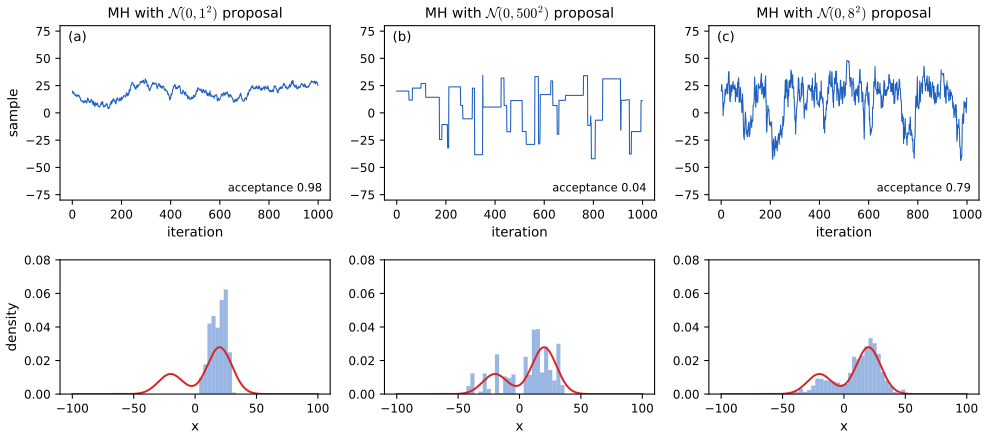
fig_12_1. Reproduces Murphy (2023), Figure 12.1. Download: PDF · SVGFilling the gap 12.2: where \(2.38^2/D\) and 0.234 come from p. 503
The book quotes the result. The acceptance-rate part can be derived exactly; the optimality part rests on a diffusion limit, which is stated.
Derivation
Set-up. Take the standardised Gaussian target \(\N(\bm 0,\bm I_D)\) and \(\tau=\ell/\sqrt D\). With \(\bm x\sim\N(\bm 0,\bm I)\) (stationarity) and \(\bm\xi\sim\N(\bm 0,\bm I)\) independent, \(\bm x'=\bm x+\tau\bm\xi\) and the log acceptance ratio is \[ \Delta=-\tfrac12\big(\|\bm x'\|^2-\|\bm x\|^2\big)=-\frac{\ell}{\sqrt D}\bm x^\T\bm\xi-\frac{\ell^2}{2D}\|\bm\xi\|^2. \] Given \(\bm\xi\), \(\bm x^\T\bm\xi\sim\N(0,\|\bm\xi\|^2)\), and \(\|\bm\xi\|^2/D\to1\) by the law of large numbers. So \(\Delta\to\N(-\ell^2/2,\ \ell^2)\) in distribution.
The acceptance rate. For \(W\sim\N(-\sigma^2/2,\sigma^2)\), \[ \E\min(1,e^W)=\Pr(W>0)+\E[e^W;W<0] \]. The first term is \(\Phi(-\sigma/2)\). For the second, \(e^w\) times the \(\N(-\sigma^2/2,\sigma^2)\) density is the \(\N(\sigma^2/2,\sigma^2)\) density (complete the square: \[ w-(w+\sigma^2/2)^2/(2\sigma^2)=-(w-\sigma^2/2)^2/(2\sigma^2) \]), so \[ \E[e^W;W<0]=\Pr_{\N(\sigma^2/2,\sigma^2)}(W<0)=\Phi(-\sigma/2) \]. Hence, by bounded convergence, the limit acceptance rate is \[ a(\ell)=2\Phi(-\ell/2). \]
The efficiency. Roberts, Gelman and Gilks (1997) show that each coordinate, with time sped up by a factor \(D\), converges to a Langevin diffusion with speed \(h(\ell)=\ell^2a(\ell)\); the larger the speed, the smaller the asymptotic variance of every chain average. The expected squared jump distance has the same limit: \[ \E\big[\|\bm x'-\bm x\|^2\min(1,e^\Delta)\big]=\E\big[\tfrac{\ell^2}{D}\|\bm\xi\|^2\min(1,e^\Delta)\big]\to\ell^2a(\ell) \]. Maximising \(\ell^2\cdot2\Phi(-\ell/2)\) numerically gives \(\ell^*=2.3812\) and \(a(\ell^*)=0.2338\). For a target with covariance \(\bm\Sigma\) the same argument after whitening gives the proposal covariance \(2.38^2\bm\Sigma/D\). Figure 12.S1 compares the limit with simulations in \(D=20\): already there the optimum is close to \(\ell=2.4\) and an acceptance rate of 0.2 to 0.3, and the curve is flat near its top, so acceptance rates between 0.15 and 0.4 lose little.
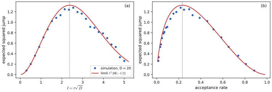
fig_12_S1. Download: PDF · SVG12.2.3.3 Composing proposals
p. 504, (12.16)–(12.17) Proposals can be mixed, \(q=\sum_kw_kq_k\) (12.16), or chained (12.17), for instance one block of variables at a time.
12.2.3.4 Data-driven MCMC
p. 504, (12.18) When the target is a posterior, the proposal may look at the data, \(q(\bm x'\given\bm x,\mathcal D)\), for example through a recognition network or part detectors mixed with a random walk (12.18). Nothing in Result 12.1 requires \(q\) to be ignorant of \(\mathcal D\): the data are fixed throughout, so any data-dependent proposal with the Hastings correction is valid. This is "generate and test": discriminative proposals generate hypotheses, the posterior ratio tests them.
12.2.3.5 Adaptive MCMC
p. 504 Tuning the proposal while the chain runs is attractive, but each adaptation must be done with care.
Filling the gap 12.3: mixtures and compositions are valid; naive adaptation is not p. 504, (12.16)–(12.17)
The book asserts both facts. Here are the proofs and a two-state counterexample to adaptation.
Derivation
Mixtures. If each kernel \(K_k\) leaves \(p^*\) invariant (\(p^*K_k=p^*\)) then \(p^*\sum_kw_kK_k=\sum_kw_kp^*=p^*\); detailed balance is linear in the kernel, so a mixture of reversible kernels is reversible. Two implementations of (12.16) are valid: (i) choose \(k\) with probability \(w_k\) and run an MH step with \(q_k\) (and \(q_k\) in the ratio), a mixture of MH kernels; (ii) propose from the mixture and use the mixture density \(q\) in the ratio, a single MH kernel.
Compositions. If \(p^*K_1=p^*\) and \(p^*K_2=p^*\) then \(p^*K_1K_2=p^*K_2=p^*\): the composition is invariant. It is generally not reversible: the adjoint of \(K_1K_2\) in \(L^2(p^*)\) is \(K_2^*K_1^*=K_2K_1\ne K_1K_2\). The systematic-scan Gibbs sampler is an example (Practice problem 12.3). The palindrome \(K_1K_2K_1\) is self-adjoint, hence reversible.
Adaptation can break invariance. Let the target be uniform on \(\{0,1\}\) and \(K_\theta\) the kernel "stay with probability \(\theta\), otherwise flip". Every \(K_\theta\) leaves the uniform distribution invariant. Now adapt: use \(\theta=0.9\) when the current state is 0 and \(\theta=0.1\) when it is 1. The resulting chain is Markov with \(\Pr(0\to1)=0.1\), \(\Pr(1\to0)=0.9\), whose stationary distribution is \((0.9,0.1)\), not \((\tfrac12,\tfrac12)\). Each kernel is valid; letting the choice depend on the state is not. Roberts and Rosenthal (2007) give sufficient conditions for adaptive schemes: diminishing adaptation (the change between successive kernels tends to zero) and containment (the kernels' convergence times stay bounded in probability). This is what the book's "faded out gradually" means; Andrieu and Thoms (2008) review practical schemes. The step-size warm-up used for Figures 12.13 and 12.14 adapts only during the warm-up and then freezes, which is always safe because the kept draws come from a fixed kernel.
See also: Result 11.18 (mixtures and compositions of transitions).
12.2.4 Initialization
p. 505 Start where \(\tilde p>0\). Starting at a mode found by an optimiser is natural, but there the gradient vanishes and gradient-based samplers start slowly; starting near (not at) the MAP estimate, or from overdispersed points when several chains are run, is common practice. Overdispersed starts are what make the between-chain diagnostics of Section 12.6.2 informative.
12.3 Gibbs sampling
12.3.1 Basic idea
p. 505, (12.19) Update each variable from its full conditional given the current values of the others, \(x_i^{s+1}\sim p(x_i\given\bm x_{-i})=p(x_i\given\bm x_{\mb(i)})\) (12.19); only the Markov blanket matters. Nodes that share no edge in the (moralised) graph are conditionally independent given the rest and can be updated together, which is the idea of graph colouring.
12.3.2 Gibbs sampling is a special case of MH
Result 12.2 (a Gibbs update is an MH step that is always accepted) p. 506, (12.20)–(12.22)
With the proposal \(q_i(\bm x'\given\bm x)=p(x_i'\given\bm x_{-i})\ind(\bm x'_{-i}=\bm x_{-i})\) (12.20), the MH ratio (12.21) equals 1 (12.22).
Proof
Write \(p(\bm x')=p(x_i'\given\bm x_{-i})p(\bm x_{-i})\) and \(p(\bm x)=p(x_i\given\bm x_{-i})p(\bm x_{-i})\), using \(\bm x'_{-i}=\bm x_{-i}\). Then \[ p(\bm x')q_i(\bm x\given\bm x')=p(x_i'\given\bm x_{-i})p(\bm x_{-i})p(x_i\given\bm x_{-i})=p(\bm x)q_i(\bm x'\given\bm x) \], so \(\alpha=1\). A full sweep is the composition of these kernels, invariant but not reversible (Filling the gap 12.3); a random-scan sweep is their mixture, reversible.
See also: Result 11.20; Filling the gap 24.16.
12.3.3 Example: Gibbs sampling for Ising models
pp. 506–508, (12.23)–(12.29), Figures 12.2–12.3 For the Ising model \(p(\bm x)\propto\exp(J\sum_{i\sim j}x_ix_j)\), \(x_i\in\{-1,+1\}\), the full conditional is \(p(x_i=+1\given\bm x_{-i})=\sigma(2J\eta_i)\) with \(\eta_i=\sum_{j\in\nbr(i)}x_j\) (12.27). With a Gaussian likelihood \(\N(y_i\given x_i,\sigma^2)\) for a noisy image it becomes \(\sigma\big(2J\eta_i+\log\psi_i(+1)/\psi_i(-1)\big)\) (12.29).
Filling the gap 12.4: the Ising full conditional, the local evidence, and why checkerboard updates are exact pp. 506–507, (12.25)–(12.29)
Derivation
Full conditional. Only the factors containing \(x_i\) survive normalisation: \(p(x_i\given\bm x_{-i})\propto\prod_{j\in\nbr(i)}e^{Jx_ix_j}=e^{Jx_i\eta_i}\). So \[ p(x_i=+1\given\bm x_{-i})=\frac{e^{J\eta_i}}{e^{J\eta_i}+e^{-J\eta_i}}=\frac{1}{1+e^{-2J\eta_i}}=\sigma(2J\eta_i). \] (In (12.25) the second product of the denominator should read \(\psi(x_i=-1,x_j)\), not \(\psi(x_i=-1,x_i)\).) If \(a_i\) neighbours agree with the current \(x_i\) and \(d_i\) disagree, \(\eta_i=x_i(a_i-d_i)\); with \(a_i=d_i\) the conditional is \(\tfrac12\).
Local evidence. For \(\psi_i(x)=\N(y_i\given x,\sigma^2)\), \[ \log\frac{\psi_i(+1)}{\psi_i(-1)}=\frac{(y_i+1)^2-(y_i-1)^2}{2\sigma^2}=\frac{2y_i}{\sigma^2}, \] so the update is \(\sigma(2J\eta_i+2y_i/\sigma^2)\): the neighbours and the pixel vote additively on the log-odds scale.
Checkerboard. Colour site \((r,c)\) by the parity of \(r+c\). Neighbours have opposite colours (on a free-boundary grid, or a torus with even side length; with an odd side the wrap-around joins two sites of the same colour). The full conditional of a black site depends only on white sites, so given all white sites the black sites are independent and \(p(\text{black}\given\text{white})=\prod_{i\text{ black}}p(x_i\given\bm x_{-i})\). Updating all black sites at once is therefore an exact block-Gibbs step, not an approximation.
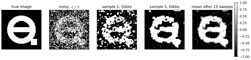
fig_12_3. Reproduces Murphy (2023), Figure 12.3. Download: PDF · SVGSee also: the mean-field solution of the same problem in Filling the gap 4.16; Gibbs sampling of the Ising model across the critical coupling in the Ising and Potts demonstration.
12.3.4 Example: Gibbs sampling for Potts models
p. 508, (12.30)–(12.32) For \(E(\bm x)=-J\sum_{i\sim j}\ind(x_i=x_j)\) the same argument gives \[ p(x_i=k\given\bm x_{-i})\propto\exp\big(J\,\#\{n\in\nbr(i):x_n=k\}\big) \] (12.32): a softmax over the neighbour counts. \(J>0\) favours agreeing with the neighbours (attractive), \(J<0\) disagreeing (repulsive). Samples are in Figure 4.18 of the Chapter 4 notes.
12.3.5 Example: Gibbs sampling for GMMs
pp. 508–510, (12.33)–(12.48), Figure 12.4 The Bayesian GMM has \(p(z=k,\bm x\given\bm\theta)=\pi_k\N(\bm x\given\bm\mu_k,\bm\Sigma_k)\) (12.33) and the conditionally conjugate prior (12.34).
12.3.5.1 Known parameters
pp. 508–509, (12.35) Alternating \(z\sim p(z\given x)\) by Bayes' rule (12.35) and \(x\sim\N(\mu_z,\sigma_z^2)\) gives correlated draws from the mixture (Figure 12.4), although ancestral sampling would give independent ones.
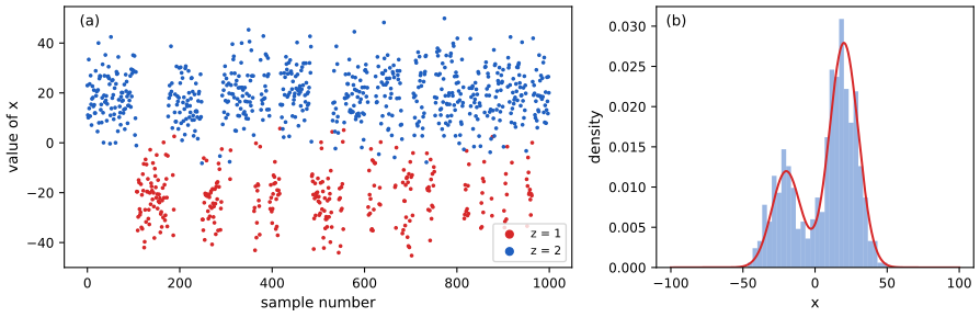
fig_12_4. Reproduces Murphy (2023), Figure 12.4. Download: PDF · SVGFilling the gap 12.5: the exact autocorrelation of the mixture Gibbs sampler p. 509, Figures 12.4 and 12.17(d)
The book says the draws are "auto correlated" and refers to Section 12.6.3. For this sampler the autocorrelation function can be computed exactly.
Derivation
The label chain. The labels \(z_1,z_2,\dots\) form a two-state Markov chain with \[ P_{jk}=\Pr(z'=k\given z=j)=\int\N(x\given\mu_j,\sigma_j^2)\,p(z=k\given x)\,\d x. \] By quadrature, \(P_{12}=0.05159\) and \(P_{21}=0.02211\) (simulation: 0.0512 and 0.0219). They satisfy \(\pi_1P_{12}=\pi_2P_{21}\) (\(0.3\times0.05159=0.7\times0.02211=0.01548\)), as detailed balance requires. The second eigenvalue is \(\lambda=1-P_{12}-P_{21}=0.9263\).
The \(x\) chain. Write \(x_t=\mu_{z_t}+\sigma\varepsilon_t\) with \(\varepsilon_t\) independent of \(z_t\), \(m=\E x=8\), \[ \var(x)=\sigma^2+\var(\mu_z)=100+40^2\cdot0.21=436 \]. For lag 1, \(z_{t+1}\) depends on \(x_t\) only, and \(\E[\mu_{z_{t+1}}\given x_t]=\E[\mu_z\given x=x_t]\), so \[ \cov(x_t,x_{t+1})=\cov\big(x_t,\E[\mu_z\given x_t]\big)=\cov(x,\mu_z)=\var(\mu_z)=336. \] For larger lags the label chain forgets geometrically: \(\E[\mu_{z_{t+\ell}}\given z_{t+1}]-m=\lambda^{\ell-1}(\mu_{z_{t+1}}-m)\) for a two-state chain, so \(\cov(x_t,x_{t+\ell})=336\lambda^{\ell-1}\). Hence \[ \rho(\ell)=\frac{336}{436}\,\lambda^{\ell-1}=0.7706\times0.9263^{\ell-1},\qquad\ell\ge1, \] (simulated lag-1 autocorrelation 0.7716), and the integrated autocorrelation time is \(1+2\rho(1)/(1-\lambda)=21.9\): 1000 Gibbs draws are worth about 46 independent ones. The decay is slow because the label switches only when \(x\) lands in the overlap of the two components.
12.3.5.2 Unknown parameters
p. 510, (12.36)–(12.48) With the parameters unknown, the Gibbs sampler cycles through \(z_i\) (12.39), \(\bm\pi\) (12.40), \(\bm\mu_k\) (12.41)–(12.45) and \(\bm\Sigma_k\) (12.46)–(12.48) (gibbs_gmm_unknown).
Filling the gap 12.6: the four full conditionals of the Bayesian GMM p. 510, (12.39)–(12.48)
Derivation
Each conditional is read off the joint (12.37)–(12.38) by keeping the factors that contain the variable.
Labels. The factors containing \(z_i\) are \(\prod_k(\pi_k\N(\bm x_i\given\bm\mu_k,\bm\Sigma_k))^{\ind(z_i=k)}\), so \(p(z_i=k\given\cdot)\propto\pi_k\N(\bm x_i\given\bm\mu_k,\bm\Sigma_k)\) (12.39); given \(\bm\theta\) the labels are independent and can be drawn in parallel.
Weights. \(\prod_i\prod_k\pi_k^{\ind(z_i=k)}\Dir(\bm\pi\given\bm\alpha)\propto\prod_k\pi_k^{N_k+\alpha_k-1}\), a \(\Dir(\bm\alpha+\bm N)\) (12.40).
Means. \(\prod_{i:z_i=k}\N(\bm x_i\given\bm\mu_k,\bm\Sigma_k)\,\N(\bm\mu_k\given\bm m_0,\bm V_0)\). The exponent is \[ -\tfrac12\bm\mu_k^\T(\bm V_0^{-1}+N_k\bm\Sigma_k^{-1})\bm\mu_k+\bm\mu_k^\T(\bm\Sigma_k^{-1}N_k\bar{\bm x}_k+\bm V_0^{-1}\bm m_0)+\const \]; completing the square gives (12.42)–(12.43). This is the known-covariance update of Section 3.4.4.1 applied to the points currently in cluster \(k\). An empty cluster (\(N_k=0\)) draws \(\bm\mu_k\) from the prior.
Covariances. \[ \prod_{i:z_i=k}\N(\bm x_i\given\bm\mu_k,\bm\Sigma_k)\IW(\bm\Sigma_k\given\bm S_0,\nu_0)\propto|\bm\Sigma_k|^{-(\nu_0+N_k+D+1)/2}\exp\big(-\tfrac12\Tr[(\bm S_0+\sum_{i:z_i=k}(\bm x_i-\bm\mu_k)(\bm x_i-\bm\mu_k)^\T)\bm\Sigma_k^{-1}]\big) \], an \(\IW(\bm S_k,\nu_0+N_k)\) (12.46)–(12.48) (Section 3.4.4.2).
Label switching. The posterior is invariant under permutations of the component labels, so it has \(K!\) symmetric modes. A well-mixing sampler visits all of them and the posterior mean of \(\bm\mu_1\) is then the average of all component means; summaries must be computed on label-invariant quantities or after relabelling. Gibbs samplers usually stay in one labelling, which is a failure to mix that happens to be convenient.
12.3.6 Metropolis within Gibbs
pp. 510–511, (12.49) When a full conditional cannot be sampled, replace the draw by one MH step that targets it: propose \(x_i'\sim q(\cdot\given x_i)\) and accept with the ratio (12.49), in which every factor not involving \(x_i\) cancels. Each such step leaves the full conditional, hence the joint, invariant (compositions).
See also: why Metropolis within Gibbs is valid.
12.3.7 Blocked Gibbs sampling
p. 511, (12.50), Figure 12.5 Single-site updates are slow when variables are strongly correlated: a move of size \(\ell\) (the conditional spread) has to cover a range \(L\) (the marginal spread). Updating correlated variables together (a block) fixes this; for an HMM, \(\bm z_{1:T}\) is drawn as one block by forwards filtering, backwards sampling (12.50).
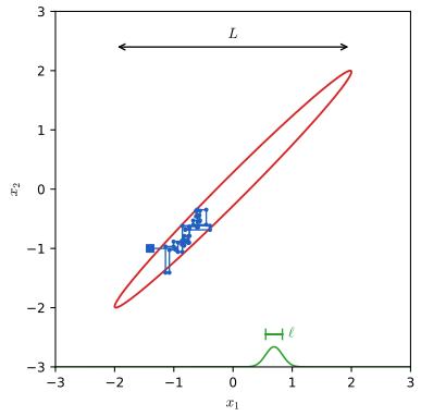
fig_12_5. Reproduces Murphy (2023), Figure 12.5. Download: PDF · SVGFilling the gap 12.7: the \(O((L/\ell)^2)\) rule, exactly p. 511
Derivation
For \(\N(\bm 0,[[1,\rho],[\rho,1]])\), \(x_1\given x_2\sim\N(\rho x_2,1-\rho^2)\). One systematic sweep is \(x_1'=\rho x_2+s\varepsilon_1\), \(x_2'=\rho x_1'+s\varepsilon_2\) with \(s=\sqrt{1-\rho^2}\), so \[ x_2'=\rho^2x_2+\rho s\varepsilon_1+s\varepsilon_2, \] an AR(1) process with coefficient \(\rho^2\) and stationary variance \((\rho^2s^2+s^2)/(1-\rho^4)=1\). Its autocorrelation is \(\rho^{2\ell}\) and its integrated autocorrelation time (Section 12.6.3) is \[ \tau=1+2\sum_{\ell\ge1}\rho^{2\ell}=\frac{1+\rho^2}{1-\rho^2}. \] With \(L=1\) and \(\ell=\sqrt{1-\rho^2}\), \((L/\ell)^2=1/(1-\rho^2)\) and \(\tau=2(L/\ell)^2-1\): the book's \(O((L/\ell)^2)\) with constant 2. For \(\rho=0.99\), \(\tau=99.5\); a run of \(2\times10^5\) sweeps gives an effective sample size of 0.99% of the draws (theory 1.005%) and lag-1 to 3 autocorrelations 0.980, 0.960, 0.941 (theory 0.980, 0.961, 0.941). Sampling \((x_1,x_2)\) as one block gives independent draws.
See also: Gibbs on a bivariate Gaussian and why about \((\sigma_{\max}/\sigma_{\min})^2\) steps are needed.
12.3.8 Collapsed Gibbs sampling
pp. 512–513, (12.51)–(12.57), Figure 12.6, Algorithm 12.2 With a conjugate prior the parameters \(\bm\pi,\bm\mu_k,\bm\Sigma_k\) can be integrated out, leaving a sampler on the labels alone. The labels become dependent, but the full conditional is the product of a prior predictive for \(z_i\) and a posterior predictive for \(\bm x_i\) given the other members of each cluster (12.53).
Algorithm 12.2 (collapsed Gibbs sampler for a mixture model) p. 513
For each \(i\) in random order: remove \(\bm x_i\)'s sufficient statistics from its cluster; for each \(k\), compute the predictive \(p_k(\bm x_i)=p(\bm x_i\given\{\bm x_j:z_j=k,j\ne i\},\bm\beta)\) and the weight \((N_{k,-i}+\alpha/K)\,p_k(\bm x_i)\); draw \(z_i\) from the normalised weights; add \(\bm x_i\)'s statistics to the chosen cluster. Implemented for 1-d clusters with a normal-inverse-gamma prior in collapsed_gibbs_gmm1d.
Filling the gap 12.8: the prior predictive of a label, and a slip in (12.56) pp. 512–513, (12.54)–(12.57)
Derivation
The Dirichlet-multinomial (12.54). With \(\bm\pi\sim\Dir(\alpha/K,\dots,\alpha/K)\), \[ p(z_{1:N}\given\alpha)=\int\prod_k\pi_k^{N_k}\,\frac{\Gamma(\alpha)}{\Gamma(\alpha/K)^K}\prod_k\pi_k^{\alpha/K-1}\,\d\bm\pi=\frac{\Gamma(\alpha)}{\Gamma(N+\alpha)}\prod_{k=1}^K\frac{\Gamma(N_k+\alpha/K)}{\Gamma(\alpha/K)}, \] because the integrand is an unnormalised \(\Dir(\bm N+\alpha/K)\) with normaliser \(\prod_k\Gamma(N_k+\alpha/K)/\Gamma(N+\alpha)\).
The ratio. \(p(z_i=k\given\bm z_{-i},\alpha)=p(\bm z\given\alpha)/p(\bm z_{-i}\given\alpha)\), where \(\bm z_{-i}\) has \(N-1\) labels and counts \(N_{j,-i}\). All factors with \(j\ne k\) cancel, leaving \[ p(z_i=k\given\bm z_{-i},\alpha)=\frac{\Gamma(N-1+\alpha)}{\Gamma(N+\alpha)}\cdot\frac{\Gamma(N_{k,-i}+1+\alpha/K)}{\Gamma(N_{k,-i}+\alpha/K)}=\frac{N_{k,-i}+\alpha/K}{N+\alpha-1}, \] using \(\Gamma(x+1)=x\Gamma(x)\). The book's final expression (12.56) prints \(N_{k,-i}+\alpha\); the middle expression of (12.56) and Algorithm 12.2 both have \(\alpha/K\), which is correct (the weights then sum to 1 over \(k\)). This ratio was confirmed against the exact enumeration of \(p(\bm z\given\alpha)\).
The predictive (12.57). Conditionally on the labels, the clusters are independent conjugate models, so \(p(\bm x_i\given\bm x_{-i},z_i=k,\bm z_{-i})=p(\bm x_i\given\mathcal D_{-i,k})\), the posterior predictive of one cluster: a Student \(t\) for the normal-inverse-gamma (or NIW) prior, with parameters that depend only on the cluster's count, sum and sum of squares. That is why removing and adding sufficient statistics (lines 2 and 7 of the algorithm) is all the bookkeeping needed. The \(\bm x_{-i}\) factor in (12.52) does not depend on \(z_i\) and drops out in (12.53).
12.4 Auxiliary variable MCMC
p. 513 Add variables \(\bm v\) so that \(p(\bm x,\bm v)\) is easier to sample than \(p(\bm x)\), sample the pair, and throw \(\bm v\) away; the \(\bm x\) draws have the right marginal.
12.4.1 Slice sampling
pp. 514–515, (12.58)–(12.60), Figures 12.7–12.8 The uniform distribution under the graph of \(\tilde p\), \(\hat p(x,v)=Z_p^{-1}\ind(0\le v\le\tilde p(x))\) (12.58), has marginal \(p(x)\) (12.59). Gibbs on it alternates \(v\sim\Unif[0,\tilde p(x)]\) (12.60) and \(x\sim\) uniform on the slice \(\{x:\tilde p(x)\ge v\}\).
Filling the gap 12.9: why the stepping-out procedure is allowed p. 515
Derivation
The slice is usually a union of intervals that cannot be computed. Neal's (2003) procedure places a window of width \(w\) at a random offset around \(x\), steps out until both ends are outside the slice, then samples uniformly in the window, shrinking it towards \(x\) after each rejected point. The result is not a uniform draw on the slice, but the kernel is reversible with respect to the uniform distribution on the slice: the probability of building a given final window from \(x\) equals that from \(x'\) whenever both lie in it, because the random offset and the step limits are chosen symmetrically, and the shrinkage rule depends on the window and the accepted point only through the slice. A kernel that is reversible for each conditional \(p(x\given v)\) leaves \(\hat p(x,v)\) invariant, so the Gibbs argument goes through. The full proof is Result 11.23. In \(D\) dimensions the text uses one height per coordinate, i.e. a slice update of each full conditional (slice_sample), which needs only the unnormalised joint.
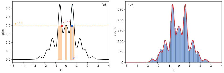
fig_12_7. Reproduces Murphy (2023), Figure 12.7. Download: PDF · SVG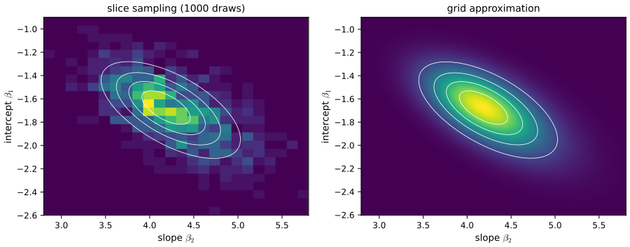
fig_12_8. Reproduces Murphy (2023), Figure 12.8. Download: PDF · SVG12.4.2 Swendsen-Wang
pp. 515–517, (12.61), Figure 12.9 For a ferromagnetic Ising model (\(J>0\)), add a bond variable \(v_e\in\{0,1\}\) per edge with the potentials (12.61). Given the spins, each agreeing edge is bonded with probability \(1-e^{-2J}\); given the bonds, every connected cluster takes a single random spin.
Filling the gap 12.10: the Swendsen-Wang conditionals, and the two versions of the cluster update pp. 515–516, (12.61)
Derivation
Marginal. For agreeing spins, \[ \Psi(\bm x_e,0)+\Psi(\bm x_e,1)=e^{-J}+(e^J-e^{-J})=e^J \]; for disagreeing spins, \(e^{-J}+0=e^{-J}\). This is \(\Psi(\bm x_e)\), so \(\sum_{\bm v}p(\bm x,\bm v)=p(\bm x)\).
Bonds given spins. The joint is a product over edges, so the bonds are conditionally independent with \[ \Pr(v_e=1\given\bm x)=\frac{(e^J-e^{-J})\ind(x_i=x_j)}{\Psi(\bm x_e)}=\begin{cases}1-e^{-2J},&x_i=x_j\\0,&x_i\ne x_j.\end{cases} \]
Spins given bonds. As a function of \(\bm x\), \(p(\bm x,\bm v)\propto\prod_{e:v_e=1}\ind(x_i=x_j)\) (the factors \(e^{-J}\) and \(e^J-e^{-J}\) do not depend on \(\bm x\) once \(\bm v\) is fixed). So \(p(\bm x\given\bm v)\) is uniform over the configurations that are constant on every cluster of the bond graph: every cluster independently takes the value \(+1\) or \(-1\) with probability \(\tfrac12\). This full update is the Gibbs step, and is what the code and the demonstration do. The book's description picks one cluster at random and gives it a random spin. That is also valid: it is a symmetric move within the set of cluster-constant configurations, so it leaves the uniform \(p(\bm x\given\bm v)\) invariant, but it moves less per sweep.
Why it mixes. Summing out \(\bm x\) gives \(p(\bm v)\propto(e^{2J}-1)^{|\bm v|}2^{c(\bm v)}\) with \(c(\bm v)\) the number of clusters: the Fortuin–Kasteleyn random-cluster model of Filling the gap 4.9. At and below the critical temperature large clusters form, and flipping a whole cluster changes the magnetisation in one sweep, a move that single-site Gibbs makes only by growing a domain wall across the lattice. On a \(32\times32\) torus at \(J_c=0.4407\), the integrated autocorrelation time of \(|m|\) is about 187 sweeps for Gibbs and 10 for Swendsen–Wang (and about 1170 against 1 for the signed magnetisation \(m\)). At \(J=0.6\), Gibbs started at all \(+1\) never left the positive mode in 1000 sweeps, while Swendsen–Wang spent 50.5% of the sweeps in each; both give \(\E|m|=0.973\), Onsager's value for the infinite lattice being 0.9736 (Figure 12.S2). With antiferromagnetic or mixed couplings the bond construction no longer produces useful clusters, as the book notes.
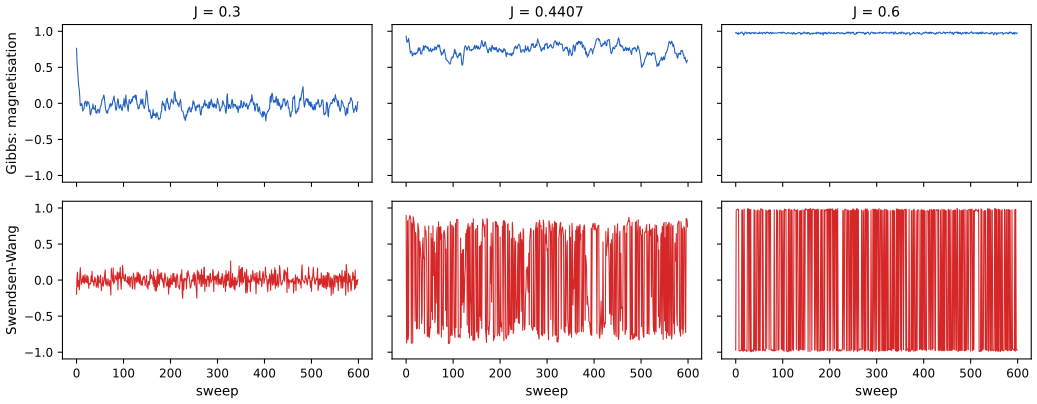
fig_12_S2. Download: PDF · SVG12.5 Hamiltonian Monte Carlo (HMC)
p. 517 HMC (Duane et al. 1987; Neal 2011) adds a momentum and uses the gradient of the log density to make long, directed moves that are still accepted with high probability.
12.5.1 Hamiltonian mechanics
pp. 517–518, (12.62)–(12.66) With position \(\th\), momentum \(\bm v\), potential \(E(\th)=-\log\tilde p(\th)\) (12.63) and kinetic energy \(K(\bm v)\) (12.64), the Hamiltonian \(H=E+K\) (12.62) is conserved by Hamilton's equations (12.65)–(12.66).
Filling the gap 12.11: the flow preserves volume, is reversible, and preserves \(e^{-H}\) p. 518
The book refers to the literature for volume preservation.
Derivation
Volume. Write \(\bm z=(\th,\bm v)\) and \(\dot{\bm z}=F(\bm z)=(\partial H/\partial\bm v,-\partial H/\partial\th)\). The divergence is \[ \nabla\cdot F=\sum_i\big(\partial^2H/\partial\theta_i\partial v_i-\partial^2H/\partial v_i\partial\theta_i\big)=0 \]. Let \(J_t=\partial\bm z(t)/\partial\bm z(0)\); then \(\dot J_t=DF\,J_t\) and by Jacobi's formula \[ \tfrac{\d}{\d t}\det J_t=\Tr(DF)\det J_t=(\nabla\cdot F)\det J_t=0 \], so \(\det J_t=\det J_0=1\) (Liouville's theorem).
Reversibility. If \(K(\bm v)=K(-\bm v)\) and \((\th(t),\bm v(t))\) solves (12.65), so does \((\th(-t),-\bm v(-t))\): running the flow forwards, flipping the momentum and running forwards again returns to the start with the momentum flipped.
Invariance. The flow conserves \(H\), hence \(e^{-H}\), and preserves volume, so it maps the distribution with density \(\propto e^{-H}\) to itself (change of variables with unit Jacobian). The full proof in Bishop's notation is Result 11.24.
12.5.2 Integrating Hamilton's equations
pp. 518–519, (12.67)–(12.74) Euler's method updates position and momentum simultaneously (12.67)–(12.68); the modified Euler method updates momentum first and then position with the new momentum (12.70)–(12.71); the leapfrog integrator does a half step of momentum, a full step of position and another half step of momentum (12.72)–(12.74).
Filling the gap 12.12: why Euler spirals out, why leapfrog does not, and the stability limit \(\eta<2\sigma\) pp. 518–519
The book says the modified method is "slightly more accurate" and leapfrog symmetrised; the harmonic oscillator \(H=\tfrac12\theta^2+\tfrac12v^2\) makes the differences exact.
Derivation
Euler. With \(\partial E/\partial\theta=\theta\): \(\theta'=\theta+\eta v\), \(v'=v-\eta\theta\), a linear map with matrix \(\begin{pmatrix}1&\eta\\-\eta&1\end{pmatrix}\), determinant \(1+\eta^2\). It multiplies \(\theta^2+v^2\) by exactly \(1+\eta^2\) at every step: the energy grows geometrically and the trajectory spirals out (Figure 12.S3a). Not volume preserving, so unusable in HMC. (In (12.69) the position update uses \(\bm v_{t+1}\), which is the modified method, not Euler's (12.68).)
Modified Euler. \(v'=v-\eta\theta\), \(\theta'=\theta+\eta v'\): matrix \(\begin{pmatrix}1-\eta^2&\eta\\-\eta&1\end{pmatrix}\) with determinant 1. It is a composition of two shears (each changes one block of variables by a function of the other), so it preserves volume in any dimension and its energy error stays bounded; but it is not symmetric, so its inverse is not obtained by flipping the momentum.
Leapfrog. Half kick, drift, half kick: three shears, so volume preserving; and palindromic, so with \(R(\theta,v)=(\theta,-v)\) the leapfrog map \(\Phi\) satisfies \(R\Phi R=\Phi^{-1}\) (time reversibility). For the oscillator, \[ \Phi=\begin{pmatrix}1-\eta^2/2&\eta\\-\eta(1-\eta^2/4)&1-\eta^2/2\end{pmatrix},\qquad\det\Phi=1,\qquad\Tr\Phi=2-\eta^2. \] The eigenvalues of a real \(2\times2\) matrix with determinant 1 lie on the unit circle iff \(|\Tr\Phi|\le2\), i.e. \(\eta\le2\); for \(\eta>2\) one eigenvalue exceeds 1 in modulus and trajectories blow up exponentially. One checks \(\Phi^\T Q\Phi=Q\) for \(Q=\diag(1-\eta^2/4,1)\), so leapfrog exactly conserves the modified energy \(\tilde H=\tfrac12(1-\eta^2/4)\theta^2+\tfrac12v^2\). Hence \(H-\tilde H=\eta^2\theta^2/8\): from \((\theta,v)=(1,0)\), the energy error oscillates between \(-\eta^2/8\) and 0, never accumulating (Figure 12.S3d). In general leapfrog is a second-order method: the global error over a fixed time is \(O(\eta^2)\).
Stability rule. For a Gaussian target with unit mass, each eigen-direction with standard deviation \(\sigma\) is an oscillator of frequency \(1/\sigma\); rescaling time gives the limit \(\eta<2\sigma_{\min}\). This is the precise form of the advice in Section 12.5.4.2 that the step size should be of the order of the narrowest width. In the demonstration the Gaussian has \(\sigma_{\min}=\sqrt{0.05}=0.224\): with \(\eta=0.46>0.447\) every trajectory diverges.
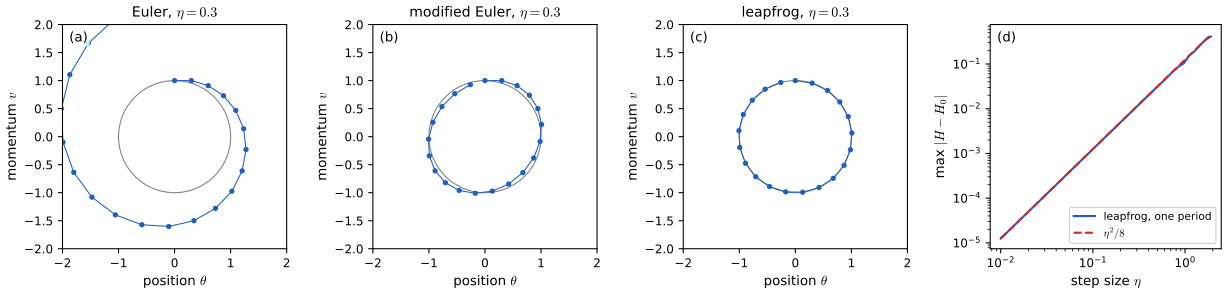
fig_12_S3. Download: PDF · SVGSee also: properties of the leapfrog integrator.
12.5.3 The HMC algorithm
pp. 519–520, (12.75)–(12.77), Algorithm 12.3 Draw a fresh momentum, run \(L\) leapfrog steps, and accept the end point with probability \(\min(1,\exp(-H^*+H))\) (12.77).
Algorithm 12.3 (Hamiltonian Monte Carlo) p. 520
For \(t=1,\dots,T\): draw \(\bm v\sim\N(\bm 0,\bm M)\); from \((\th_{t-1},\bm v)\) do a half step of momentum, \(L-1\) alternating full steps of position and momentum, a full step of position and a final half step of momentum; accept the end point \((\th^*,\bm v^*)\) with probability \(\min(1,e^{-H(\th^*,\bm v^*)+H(\th_{t-1},\bm v)})\). A trajectory whose energy error is huge (more than 1000 here) or not finite is a divergence, rejected and counted (hmc).
Filling the gap 12.13: HMC satisfies detailed balance, and the sign of \(\bm\Sigma\) pp. 519–520, (12.75)–(12.77)
Derivation
Two steps. HMC alternates (i) a Gibbs step on the momentum, \(\bm v\sim p(\bm v\given\th)=\N(\bm 0,\bm M)\), which leaves \(\pi(\th,\bm v)\propto e^{-H}\) invariant; and (ii) an MH step with the deterministic proposal \(\Psi=R\circ\Phi^L\) (leapfrog \(L\) times, then flip the momentum). By Filling the gap 12.12, \(\Psi\) preserves volume and is an involution: \(\Psi(\Psi(\bm z))=R\Phi^LR\Phi^L(\bm z)=\Phi^{-L}\Phi^L(\bm z)=\bm z\).
Detailed balance for an involution. The kernel moves \(\bm z\) to \(\Psi(\bm z)\) with probability \(a(\bm z)=\min(1,\pi(\Psi(\bm z))/\pi(\bm z))\) and stays otherwise. For bounded \(f,g\), the moving part contributes \(\int f(\bm z)g(\Psi(\bm z))\min(\pi(\bm z),\pi(\Psi(\bm z)))\d\bm z\). Substituting \(\bm z=\Psi(\bm w)\) (unit Jacobian, \(\Psi(\bm z)=\bm w\)) turns it into \(\int f(\Psi(\bm w))g(\bm w)\min(\pi(\Psi(\bm w)),\pi(\bm w))\d\bm w\): the expression is symmetric in \(f,g\), which is detailed balance. Because the next step resamples the momentum and \(K\) is even, the flip \(R\) changes nothing in practice. Integrating out \(\bm v\) gives (12.76): the \(\th\)-marginal is \(p\). The full argument is Result 11.26.
Why a fresh momentum. Along a trajectory \(E(\th)\le H\); without refreshing, the chain could never reach states of higher energy (the book's argument on p. 520). Refreshing is also what makes the chain irreducible.
The matrix \(\bm\Sigma\). With \(K=\tfrac12\bm v^\T\bm\Sigma^{-1}\bm v\) (12.64) the momentum is \(\bm v\sim\N(\bm 0,\bm\Sigma)\) and the position update is \(\eta\bm\Sigma^{-1}\bm v\). Then \(\bm\Sigma\) is the mass matrix and \(\bm\Sigma^{-1}\) the inverse mass. Two places of the text are inconsistent with this: (12.75) and the paragraph after Algorithm 12.3 write \(\tfrac12\bm v^\T\bm\Sigma\bm v\), and Section 12.5.4.3 calls \(\bm\Sigma\) the inverse mass and sets it to the posterior covariance. The correct recommendation is inverse mass \(\bm M^{-1}\approx\cov_p(\th)\) (equivalently \(\bm M\approx\) the posterior precision): with that choice, a Gaussian target becomes an isotropic oscillator and the stability limit \(\eta<2\) holds in every direction.
12.5.4 Tuning HMC
pp. 520–521 Three choices remain: the number of steps \(L\), the step size \(\eta\) and the mass matrix.
12.5.4.1 Choosing the number of steps using NUTS
p. 520 Too few steps give a diffusive random walk (preset 3 of the demonstration: \(L=1\)); too many waste work when the trajectory turns back. The no-U-turn sampler (Hoffman and Gelman 2014) doubles the trajectory until it starts to turn back and samples a point from it in a way that keeps detailed balance. Here a fixed \(L\) or an \(L\) uniform on \(\{1,\dots,L_{\max}\}\) is used (random \(L\) avoids resonances with periodic orbits).
12.5.4.2 Choosing the step size
pp. 520–521 The step must be below the stability limit of the narrowest direction (Filling the gap 12.12). In practice it is adapted during warm-up towards a target acceptance probability; the code moves \(\log\eta\) by \((a_t-0.9)/\sqrt t\) for 300 warm-up iterations, where \(a_t\) is the acceptance probability, and then freezes it (hmc_warmup).
12.5.4.3 Choosing the covariance (inverse mass) matrix
p. 521 Set the inverse mass to an estimate of the posterior covariance from warm-up draws (see Filling the gap 12.13 for which matrix is which); NeuTra HMC learns a flow that whitens the target instead.
12.5.5 Riemann manifold HMC
p. 521, (12.78)–(12.80) A position-dependent metric \(\bm G(\th)\) (the Hessian (12.78) or the Fisher information (12.79)) adapts the mass to the local curvature. The kinetic energy \(\tfrac12\log((2\pi)^D|\bm G(\th)|)+\tfrac12\bm v^\T\bm G(\th)^{-1}\bm v\) (12.80) is then the negative log density of \(\bm v\sim\N(\bm 0,\bm G(\th))\) including its normaliser, which now depends on \(\th\) and must be kept so that the \(\th\)-marginal stays \(p\). (In (12.80) the quadratic form should involve \(\bm G^{-1}\), for the same reason as in Filling the gap 12.13.) The Hamiltonian is no longer separable, and the generalised leapfrog needs implicit fixed-point steps.
12.5.6 Langevin Monte Carlo (MALA)
pp. 521–522, (12.81)–(12.83), Algorithm 12.4 HMC with \(L=1\) is the Metropolis-adjusted Langevin algorithm; without the accept step it is the unadjusted Langevin algorithm (ULA), a discretisation of the Langevin diffusion \(\d\th_t=-\nabla E(\th_t)\d t+\sqrt2\,\d\bm B_t\) (12.83).
Algorithm 12.4 (Langevin Monte Carlo) p. 522
Draw \(\bm v\sim\N(\bm 0,\bm\Sigma)\); set \(\th^*=\th-\tfrac{\eta^2}{2}\bm\Sigma^{-1}\nabla E(\th)+\eta\bm\Sigma^{-1}\bm v\) and \(\bm v^*=\bm v-\tfrac\eta2\nabla E(\th)-\tfrac\eta2\nabla E(\th^*)\); accept \(\th^*\) with probability \(\min(1,e^{-H(\th^*,\bm v^*)+H(\th,\bm v)})\).
Filling the gap 12.14: MALA is one leapfrog step; the Langevin diffusion has stationary density \(p\); ULA is biased pp. 521–522
Derivation
MALA as MH. Take \(\bm\Sigma=\bm I\), \(\bm g=\nabla\log p=-\nabla E\). The proposal \(\th^*=\th+\tfrac{\eta^2}{2}\bm g(\th)+\eta\bm v\) has density \[ q(\th^*\given\th)=\N(\th^*\given\th+\tfrac{\eta^2}{2}\bm g(\th),\eta^2\bm I)\propto e^{-\|\bm v\|^2/2} \]. For the reverse move, \[ \th-\th^*-\tfrac{\eta^2}{2}\bm g(\th^*)=-\eta\bm v-\tfrac{\eta^2}{2}(\bm g(\th)+\bm g(\th^*))=-\eta\bm v^* \], so \(q(\th\given\th^*)\propto e^{-\|\bm v^*\|^2/2}\) with the same constant. Hence \[ \frac{p(\th^*)q(\th\given\th^*)}{p(\th)q(\th^*\given\th)}=\exp\big(-E(\th^*)-\tfrac12\|\bm v^*\|^2+E(\th)+\tfrac12\|\bm v\|^2\big)=e^{-H(\th^*,\bm v^*)+H(\th,\bm v)}: \] the HMC acceptance with one leapfrog step is exactly the Hastings ratio of the Langevin proposal (checked numerically on a random target).
The diffusion. The density \(\rho_t\) of \(\d\th=\nabla\log p\,\d t+\sqrt2\,\d\bm B\) obeys the Fokker–Planck equation \[ \partial_t\rho=-\nabla\cdot(\rho\nabla\log p)+\Delta\rho=\nabla\cdot\big(\rho\nabla\log(\rho/p)\big) \]. At \(\rho=p\) the right side vanishes, so \(p\) is stationary; and \(\tfrac{\d}{\d t}\KL(\rho_t\|p)=-\int\rho_t\|\nabla\log(\rho_t/p)\|^2\le0\).
The time step. Euler–Maruyama with step \(h\) is \(\th+h\nabla\log p(\th)+\sqrt{2h}\,\bm\epsilon\), which is (12.82) with \(h=\eta^2/2\). The book's "set \(\eta=\sqrt2\)" corresponds to \(h=1\); the continuous-time limit is \(h\to0\).
ULA is biased. For \(p=\N(m,s^2)\), ULA is \(\theta'-m=(1-h/s^2)(\theta-m)+\sqrt{2h}\epsilon\), an AR(1) with stationary variance \[ \frac{2h}{1-(1-h/s^2)^2}=\frac{s^2}{1-h/(2s^2)}\qquad(h<2s^2), \] larger than \(s^2\) for every \(h>0\). The accept step of MALA removes this bias; ULA trades it for never rejecting. Figure 12.S4 shows the closed form against simulation.
12.5.7 Connection between SGD and Langevin sampling
pp. 522–523, (12.84)–(12.92) The minibatch noise of SGD has mean zero and covariance \(\tfrac\eta B\bm D(\th)\) after scaling (12.86)–(12.91), so SGD behaves like a Langevin sampler at temperature proportional to \(\eta/B\) (12.92).
Filling the gap 12.15: the moments of the minibatch gradient, and the effective temperature pp. 522–523
Derivation
Which loss. (12.84) defines \(\mathcal L\) as a sum over \(N\) examples, but (12.88) and (12.91) need it to be the average \(\mathcal L=\tfrac1N\sum_n\mathcal L_n\): with the sum, \(\E[\nabla_B\mathcal L]=\tfrac1N\nabla\mathcal L\). Use the average below.
Moments. With indices \(i_1,\dots,i_B\) drawn uniformly with replacement, \(\nabla_B\mathcal L=\tfrac1B\sum_j\bm g_{i_j}\) with \(\bm g_n=\nabla\mathcal L_n\) is an average of \(B\) independent copies of \(\bm g_I\), \(I\sim\Unif\{1..N\}\). So \(\E\nabla_B\mathcal L=\tfrac1N\sum_n\bm g_n=\nabla\mathcal L\) and \(\cov(\nabla_B\mathcal L)=\cov(\bm g_I)/B=\bm D(\th)/B\) with \(\bm D=\tfrac1N\sum_n\bm g_n\bm g_n^\T-\nabla\mathcal L\nabla\mathcal L^\T\) (12.91). Without replacement the covariance is multiplied by \((N-B)/(N-1)\).
Matching an SDE. The SGD step is \(-\eta\nabla\mathcal L+\eta(\nabla\mathcal L-\nabla_B\mathcal L)\), with noise covariance \(\eta^2\bm D/B\). The Euler–Maruyama step of size \(\eta\) for \(\d\th=-\nabla\mathcal L\,\d t+\bm C^{1/2}\d\bm B\) has noise covariance \(\eta\bm C\); matching gives \(\bm C=\tfrac\eta B\bm D\), which is (12.92). Li, Tai and E (2017) show this SDE is a weak first-order approximation of SGD over finite time horizons.
Temperature. Langevin dynamics for \(p_T\propto e^{-\mathcal L/T}\) is \(\d\th=-\nabla\mathcal L\,\d t+\sqrt{2T}\,\d\bm B\). If \(\bm D\approx d\bm I\), matching \(2T=\eta d/B\) gives \(T=\eta d/(2B)\): the temperature is proportional to \(\eta/B\), as the book says, with the gradient-noise level \(d\) as the constant. Since \(\bm D\) is not isotropic in general (and depends on \(\th\)), SGD is not exactly a tempered posterior sampler; this is why SGLD (Section 12.7.1) adds its own isotropic noise. The two moment formulas were confirmed by enumerating all minibatch draws on a small problem.
12.5.8 Applying HMC to constrained parameters
pp. 523–524, (12.93), Figure 12.10 HMC needs continuous, unconstrained parameters. Discrete latents are summed out (for a mixture, (12.93); for an HMM, by the forwards algorithm), and constrained parameters are mapped to \(\R^D\) by a bijection, adding the log Jacobian to the log density. Throughout this chapter \(\sigma\) is sampled as \(s=\log\sigma\) with the term \(+s\) (unigauss_logp).
See also: transforming a restricted variable needs the Jacobian.
12.5.9 Speeding up HMC
p. 524 Two costs dominate: bad geometry (handled by the mass matrix, Section 12.5.4.3, or reparameterisation, Section 12.6.5) and the \(O(N)\) cost of each gradient (handled by the stochastic-gradient methods of Section 12.7).
12.6 MCMC convergence
pp. 524–525, Figure 12.11 The uniform distribution on \(\{0,\dots,20\}\) is sampled by proposing \(\pm1\) with probability \(\tfrac12\) each and rejecting moves off the ends. Even this small chain needs hundreds of steps to forget its start.
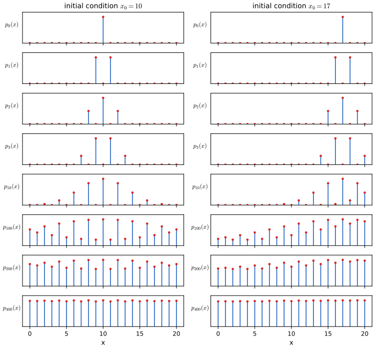
fig_12_11. Reproduces Murphy (2023), Figure 12.11. Download: PDF · SVGFilling the gap 12.16: the walk of Figure 12.11 solved exactly, and why both starts are equally far from uniform pp. 524–525
Derivation
Folding a cycle. Let \(Y_t\) be the simple random walk on the cycle \(\mathbb Z_{42}\) and fold it: \(X=Y\) if \(Y\le20\), \(X=41-Y\) otherwise. A step from \(Y=0\) to \(41\) folds to staying at 0, and a step from \(20\) to \(21\) folds to staying at 20; every other step moves \(X\) by \(\pm1\). So \(X_t\) is exactly the chain of the figure.
Spectrum. The cycle walk has eigenvalues \(\cos(2\pi j/42)\); the eigenfunctions invariant under \(y\mapsto41-y\), \(\cos(\pi k(y+\tfrac12)/21)\), pass to the folded chain. So the transition matrix \(T\) has eigenvalues \(\lambda_k=\cos(\pi k/21)\), \(k=0,\dots,20\), and the numerical eigenvalues agree: \(1\), \(0.98883\), ..., \(-0.98883\). The most negative eigenvalue is as large in modulus as the second largest: the chain is nearly periodic (it almost alternates between even and odd states, broken only by the holding at the ends).
Distance from uniform. The cycle walk at time \(t\) lives on the states of parity \(y_0+t\), and \(y\) and \(41-y\) have opposite parities, so folding never adds two non-zero masses: the total variation distance of \(X_t\) from uniform depends only on the cycle distribution, which is a translate of the same distribution for every start. Hence \(\|p_t-\Unif\|_\TV\) is the same from every starting state: 0.653, 0.207, 0.067 and 0.0071 at \(t=10,100,200,400\), and it first drops below 0.01 at \(t=370\) from all 21 starts. The two columns of Figure 12.11 look different but are equally converged.
12.6.1 Mixing rates of Markov chains
pp. 525–526, (12.94)–(12.96), Figure 12.12 The mixing time \(\tau_\epsilon=\max_{x_0}\min\{t:\|\delta_{x_0}T^t-p^*\|_1\le\epsilon\}\) (12.94)–(12.95) is governed by the spectral gap and by the conductance \(\phi\) (12.96), the smallest probability flow out of a set relative to its mass.
Filling the gap 12.17: the spectral bound, the absolute gap, and the conductance (Cheeger) inequalities pp. 525–526, (12.96)
The book states \(\tau_\epsilon=O(\gamma^{-1}\log(n/\epsilon))\) with \(\gamma=\lambda_1-\lambda_2\), and \(\tau_\epsilon\le O(\phi^{-2}\log(n/\epsilon))\). Both need care.
Derivation
Spectral bound. Let \(T\) be reversible with respect to \(\pi\) on \(n\) states. Then \(T\) is self-adjoint in \(L^2(\pi)\) and has an orthonormal eigenbasis \(f_1=1,f_2,\dots,f_n\) with real eigenvalues \(1=\lambda_1>\lambda_2\ge\dots\ge\lambda_n\ge-1\), and \(T^t(x,y)/\pi(y)=\sum_k\lambda_k^tf_k(x)f_k(y)\). By Cauchy–Schwarz, \[ 4\|T^t(x,\cdot)-\pi\|_\TV^2\le\sum_y\pi(y)\Big(\frac{T^t(x,y)}{\pi(y)}-1\Big)^2=\sum_{k\ge2}\lambda_k^{2t}f_k(x)^2\le\lambda_*^{2t}\Big(\frac1{\pi(x)}-1\Big), \] where \(\lambda_*=\max(|\lambda_2|,|\lambda_n|)\) and \(\sum_kf_k(x)^2=1/\pi(x)\). So \[ \|T^t(x,\cdot)-\pi\|_\TV\le\tfrac12\lambda_*^t\sqrt{(1-\pi(x))/\pi(x)}, \] and with the absolute gap \(\gamma_*=1-\lambda_*\) and \(\lambda_*^t\le e^{-\gamma_*t}\), \(\tau_\epsilon\le\gamma_*^{-1}\log\big(1/(2\epsilon\sqrt{\pi_{\min}})\big)\), which is \(O(\gamma_*^{-1}\log(n/\epsilon))\) when \(\pi_{\min}\asymp1/n\). The gap \(\lambda_1-\lambda_2\) of the book is not enough: the walk of Figure 12.11 has \(\lambda_2=0.98883\) but also \(\lambda_{21}=-0.98883\), and a chain with \(\lambda_n=-1\) is periodic and never converges. A lazy chain \(\tfrac12(I+T)\) has all eigenvalues in \([0,1]\), and then the two gaps agree. For the walk, the bound gives \(\|p_t-\pi\|_\TV<0.01\) once \(t\ge482\); the exact time is 370 (Figure 12.S5).
Conductance. The flow out of \(S\) must be weighted by the stationary probability: \[ \phi=\min_{S:\,0<\pi(S)\le1/2}\frac{\sum_{x\in S,x'\notin S}\pi(x)T(x\to x')}{\pi(S)}. \] ((12.96) omits \(\pi(x)\) in the numerator and allows \(\pi(S)=0\).) For a reversible chain, Cheeger's inequality reads \(\phi^2/2\le1-\lambda_2\le2\phi\) (Lawler and Sokal 1988; Jerrum and Sinclair 1989). The right inequality has a short proof: with \(f=\ind_S\), the Dirichlet form \[ \mathcal E(f,f)=\tfrac12\sum_{x,y}\pi(x)T(x,y)(f(x)-f(y))^2 \] equals the flow \(Q(S,S^c)\), and \(\var_\pi f=\pi(S)(1-\pi(S))\ge\pi(S)/2\); since \(1-\lambda_2=\min_f\mathcal E(f,f)/\var_\pi f\), we get \(1-\lambda_2\le2Q(S,S^c)/\pi(S)\). The left inequality (a small conductance is the only obstruction) needs a longer argument. Combined with the spectral bound (for a lazy chain), \(\tau_\epsilon=O(\phi^{-2}\log(n/\epsilon))\). For the walk, \(\phi=0.05\) (the set \(\{0,\dots,9\}\)), and indeed \(0.00125\le1-\lambda_2=0.0112\le0.1\).
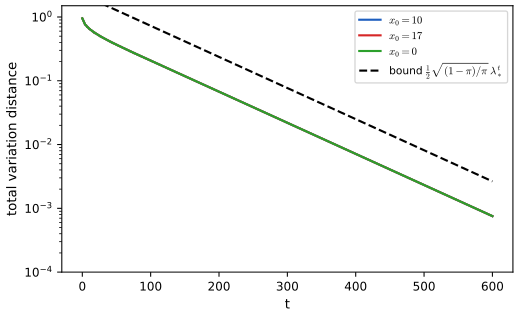
fig_12_S5. Download: PDF · SVG12.6.2 Practical convergence diagnostics
p. 526 Mixing times are rarely computable, and convergence cannot be certified in general; diagnostics can only detect some failures. The recommended practice is to run several chains from overdispersed starts and compare them.
12.6.2.1 Trace plots
pp. 526–528, Figures 12.13–12.16 The model is \(y_i\sim\N(\alpha,\sigma^2)\) with only \(y=(-1,1)\). With the diffuse prior \(\alpha\sim\N(0,1000^2)\), \(\sigma\sim\mathrm{Expon}(10^{-4})\), the posterior is nearly as diffuse as the prior; with \(\alpha\sim\N(1,10^2)\), \(\sigma\sim\mathrm{Expon}(1)\) it is well behaved. Three HMC chains (unit mass, \(L=10\), step size tuned during 300 warm-up iterations, 500 kept draws, on \((\alpha,\log\sigma)\)) start from prior draws.
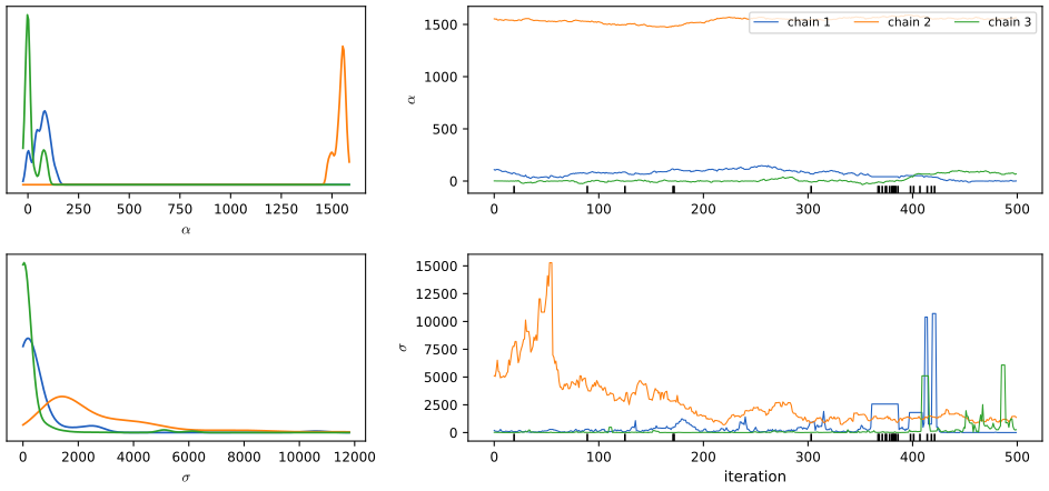
fig_12_13. Reproduces Murphy (2023), Figure 12.13. Download: PDF · SVG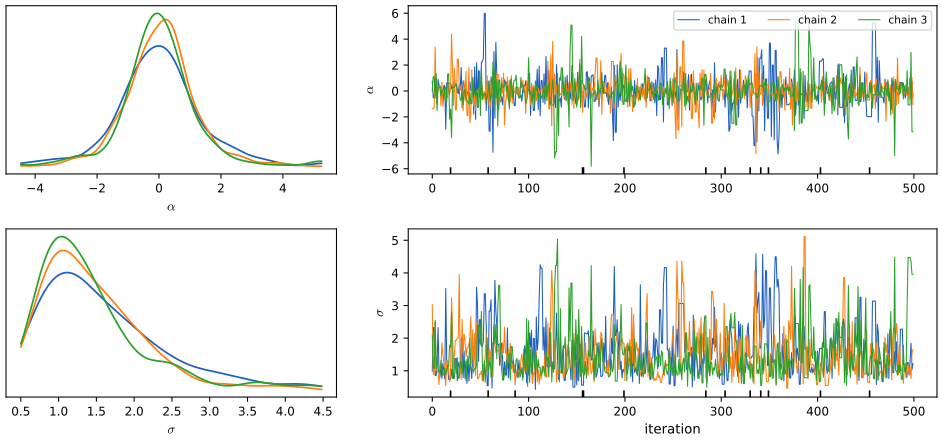
fig_12_14. Reproduces Murphy (2023), Figure 12.14. Download: PDF · SVGUnlike the book's run, this sampler reports a few divergences under both priors (24 under the diffuse and 13 under the sensible prior, out of 1500): all occur where \(\sigma\) is small, a funnel-shaped region of the \((\alpha,\log\sigma)\) posterior (Section 12.6.5) where the tuned step is too large. What separates the two runs here is the mixing in \(\alpha\), which the diagnostics below detect.
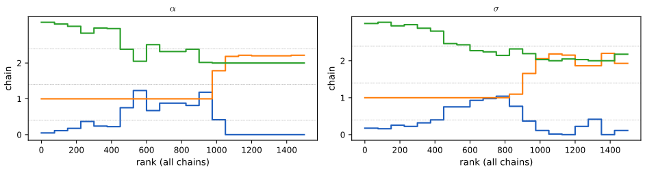
fig_12_13. Reproduces Murphy (2023), Figure 12.15. Download: PDF · SVG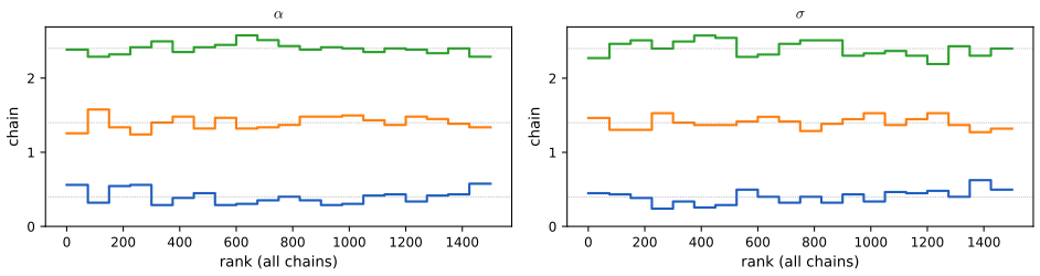
fig_12_14. Reproduces Murphy (2023), Figure 12.16. Download: PDF · SVG12.6.2.2 Estimated potential scale reduction (EPSR)
pp. 528–529, (12.97)–(12.100) With \(M\) chains of length \(N\), \(B\) (12.97) is \(N\) times the variance of the chain means and \(W\) (12.98) the average within-chain variance; \(\hat V^+=\tfrac{N-1}{N}W+\tfrac1NB\) (12.99) and \(\hat R=\sqrt{\hat V^+/W}\) (12.100). Split-\(\hat R\) halves each chain first. For the mixture samplers of Figures 12.1 and 12.4 (four chains of 1000 from \(20,-40,5,60\)) the values are 2.313 (\(\tau=1\)), 1.027 (\(\tau=500\)), 1.040 (\(\tau=8\)) and 1.004 (Gibbs); the book's are 1.493, 1.039, 1.005 and 1.007, from different starting points. Both flag \(\tau=1\); with these starts \(\tau=8\) is also flagged by the 1.01 rule.
Filling the gap 12.18: what \(\hat V^+\) estimates, and why \(\hat R\approx1+1/(2N_{\text{eff}})\) even for a perfect chain pp. 528–529
Derivation
Independent draws. If all \(MN\) draws were independent with variance \(\sigma^2\), then \(\E s_m^2=\sigma^2\), so \(\E W=\sigma^2\), and \(\E[B/N]=\var(\bar x_{\cdot m})=\sigma^2/N\). Hence \(\E\hat V^+=\tfrac{N-1}{N}\sigma^2+\tfrac{\sigma^2}N=\sigma^2\): \(\hat V^+\) is unbiased.
Unmixed chains. If the chains started far apart and have not mixed, the chain means differ by more than sampling error, \(B\) is inflated and \(\hat V^+\) overestimates \(\sigma^2\), while each chain has explored only part of the target so \(W\) underestimates it. Both push \(\hat R\) above 1; that is the design.
Stationary but correlated chains. With integrated autocorrelation time \(\tau\), \(\var(\bar x_{\cdot m})\approx\sigma^2\tau/N\) and \(\E s_m^2\approx\sigma^2(1-\tau/N)\) (the sample variance about a noisy mean loses \(\var\bar x\)). Then \[ \hat R^2\approx\frac{N-1}{N}+\frac{\tau}{N(1-\tau/N)}\approx1+\frac{\tau-1}{N},\qquad\hat R\approx1+\frac{\tau-1}{2N}\approx1+\frac1{2N_{\text{eff}}}, \] with \(N_{\text{eff}}=N/\tau\) the effective size of one chain. So the recommended threshold \(\hat R<1.01\) (Vehtari et al. 2021) also demands at least about 50 effective draws per chain, even when the chains are perfectly stationary. Four stationary AR(1) chains with coefficient 0.9 (\(\tau=19\)) and \(N=1000\) give an average \(\hat R\) of 1.009 over 300 replications, as predicted.
12.6.3 Effective sample size
pp. 529–531, (12.101)–(12.110), Figure 12.17 Correlated draws inflate the variance of a chain average by the integrated autocorrelation time \(\rho=1+2\sum_{\ell\ge1}\rho(\ell)\) (12.107), so \(N\) draws are worth \(N_{\text{eff}}=N/\rho\) (12.109); with \(M\) chains, \(NM/(1+2\sum_{\ell=1}^L\hat\rho(\ell))\) (12.110).
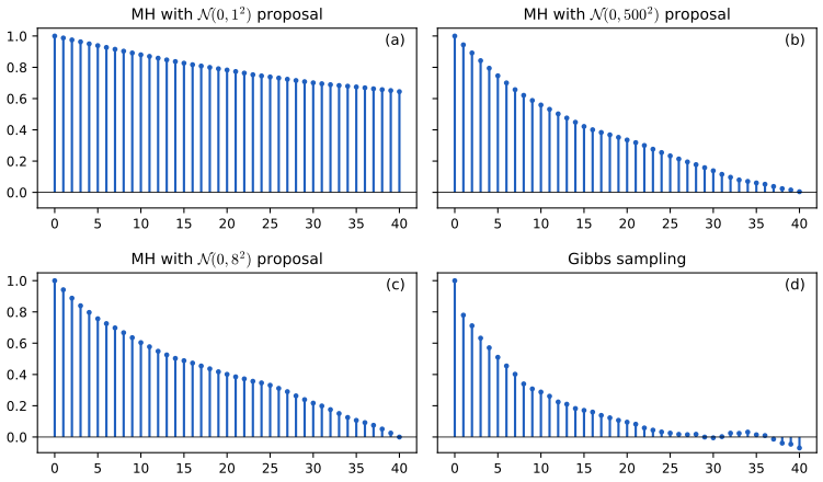
fig_12_17. Reproduces Murphy (2023), Figure 12.17. Download: PDF · SVGFilling the gap 12.19: the exact finite-\(N\) variance and the truncation of the sum pp. 530–531, (12.105)–(12.110)
Derivation
For a stationary sequence with variance \(\sigma^2\) and autocorrelation \(\rho(\ell)\), count the pairs \((i,j)\) with \(|i-j|=\ell\): there are \(N\) with \(\ell=0\) and \(2(N-\ell)\) with each \(\ell\ge1\). Hence, exactly, \[ \var(\bar x)=\frac{\sigma^2}{N}\Big[1+2\sum_{\ell=1}^{N-1}\Big(1-\frac\ell N\Big)\rho(\ell)\Big]. \] If \(\sum_\ell|\rho(\ell)|<\infty\), dominated convergence gives \(N\var(\bar x)\to\sigma^2\big(1+2\sum_{\ell\ge1}\rho(\ell)\big)\), which is (12.106)–(12.109); the book's step replaces the weights \(1-\ell/N\) by 1. For AR(1) with coefficient \(\varphi\), \(\rho(\ell)=\varphi^\ell\) and the time is \((1+\varphi)/(1-\varphi)\). Estimated autocorrelations at large lags are pure noise with standard error about \(1/\sqrt N\), and summing all of them gives an estimator whose variance does not vanish; hence the truncation. The rule used here (and in the demonstration) stops before the first lag at which the chain-averaged estimate is not positive; Geyer (1992) proposed the more robust "initial positive sequence", which sums pairs \(\rho(2k)+\rho(2k+1)\) while they are positive and is the basis of the rank-normalised estimator of Vehtari et al. (2021).
See also: the error of a chain average; Result 11.2.
12.6.4 Improving speed of convergence
pp. 531–532 Remedies when \(\hat R\) is large or \(N_{\text{eff}}\) small: reparameterise (Section 12.6.5), block (Section 12.3.7), integrate variables out (Section 12.3.8), add auxiliary variables (Section 12.4), adapt the proposal (Section 12.2.3.5).
12.6.5 Non-centered parameterizations and Neal's funnel
pp. 532–533, (12.111)–(12.115), Figure 12.18 The funnel \(\nu\sim\N(0,3^2)\), \(x\given\nu\sim\N(0,e^{\nu})\) (variance \(e^\nu\)) has a wide mouth and a narrow neck; the non-centred version samples two independent Gaussians \((z,\nu)\) and sets \(x\) deterministically.
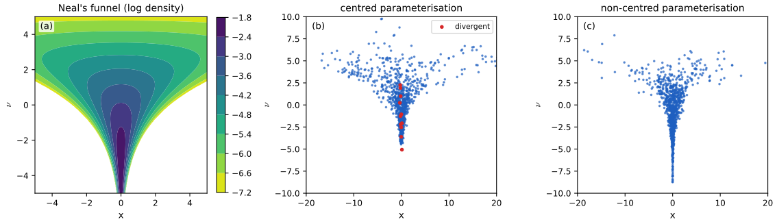
fig_12_18. Reproduces Murphy (2023), Figure 12.18. Download: PDF · SVGFilling the gap 12.20: the non-centred model is the same model (with \(e^{\nu/2}\)), and why the neck causes divergences pp. 532–533
Derivation
Equivalence. Let \(z\sim\N(0,1)\) and \(\nu\sim\N(0,9)\) be independent and \(x=ze^{\nu/2}\). The map \((z,\nu)\mapsto(x,\nu)\) has Jacobian \(\partial x/\partial z=e^{\nu/2}\), so \[ p(x,\nu)=\N(\nu\given0,9)\,\N(xe^{-\nu/2}\given0,1)\,e^{-\nu/2}=\N(\nu\given0,9)\,\N(x\given0,e^\nu), \] which is (12.111)–(12.112) with \(e^\nu\) a variance. The book's (12.115) writes \(x=z\exp(\nu)\); that would give variance \(e^{2\nu}\), a different funnel. The figure (and Neal's original) use the standard deviation \(e^{\nu/2}\).
Why the neck is hard. Given \(\nu\), \(-\log p\) is quadratic in \(x\) with curvature \(e^{-\nu}\): the conditional standard deviation is \(e^{\nu/2}\). By the stability limit of Filling the gap 12.12, a fixed leapfrog step \(\eta\) is unstable wherever \(e^{\nu/2}<\eta/2\), i.e. \(\nu<2\log(\eta/2)\); for \(\eta=0.2\) that is \(\nu<-4.6\), a region of prior probability \(\Phi(-4.6/3)=6.3\%\). Trajectories that enter it explode and are flagged as divergences, so the centred chain rarely gets below \(-5\) and its \(\nu\)-marginal is biased upwards. In \((z,\nu)\) the target is an axis-aligned Gaussian with standard deviations 1 and 3, and any \(\eta<2\) is stable everywhere. The same geometry appears between a group-level scale and the group effects of every hierarchical model (the non-centred eight-schools model).
12.7 Stochastic gradient MCMC
p. 533, (12.116)–(12.119) Write the energy as a sum over data, \(E(\th)=\sum_nE_n(\th)\) with \(E_n=-\log p(\bm x_n\given\th)-\tfrac1N\log p_0(\th)\) (12.119). Every full gradient costs \(O(N)\).
12.7.1 Stochastic gradient Langevin dynamics (SGLD)
p. 533, (12.120)–(12.123) SGLD (Welling and Teh 2011) replaces the gradient in ULA by the unbiased minibatch estimate \(\hat{\bm g}=\tfrac NB\sum_{n\in\mathcal B_t}\nabla E_n\) (12.122): \(\th_{t+1}=\th_t-\eta_t\hat{\bm g}(\th_t)+\sqrt{2\eta_t}\,\bm\epsilon_t\) (12.123), with no accept step. With decreasing steps the discretisation and gradient noise vanish asymptotically; with a constant step the chain is biased.
12.7.2 Preconditioning
p. 534 As in optimisation, a preconditioner (Fisher information, an RMSprop-style diagonal, or Adam-style moments) rescales the gradient. For the dynamics to keep the right stationary density, a position-dependent preconditioner \(\bm G(\th)\) also needs a correction drift \(\nabla\cdot\bm G(\th)\) (Ma, Chen and Fox 2015), which diagonal schemes often drop.
12.7.3 Reducing the variance of the gradient estimate
pp. 534–535, (12.124)–(12.127), Algorithm 12.5 A control variate at a reference point \(\hat\th\) gives \[ \hat\nabla_{\text{cv}}E(\th)=\nabla E(\hat\th)+\tfrac NB\sum_{n\in S_t}(\nabla E_n(\th)-\nabla E_n(\hat\th)) \] (12.124) (SGLD-CV); SVRG-LD refreshes the reference every \(\tau\) steps (12.127).
Algorithm 12.5 (SVRG Langevin descent) p. 535
Every \(\tau\) steps set \(\tilde\th=\th_t\) and \(\tilde{\bm g}=\sum_n\nabla E_n(\tilde\th)\) (line 5 of the book omits the \(\nabla\)); otherwise draw a minibatch and set \(\bm g_t=\tilde{\bm g}+\tfrac NB\sum_{n\in\mathcal B_t}(\nabla E_n(\th_t)-\nabla E_n(\tilde\th))\) and \(\th_{t+1}=\th_t-\eta\bm g_t+\sqrt{2\eta}\,\bm\epsilon_t\) (sgld_family, method="svrg").
Filling the gap 12.21: unbiasedness and variance of the three gradient estimates pp. 533–535
Derivation
Unbiased. With indices drawn uniformly with replacement, \[ \E\big[\tfrac NB\sum_{j=1}^B\nabla E_{I_j}(\th)\big]=\tfrac NB\cdot B\cdot\tfrac1N\sum_n\nabla E_n(\th)=\nabla E(\th) \], proving (12.122); applying this to \(\nabla E_n(\th)-\nabla E_n(\hat\th)\) gives (12.125)–(12.126).
Variance. \(\cov(\hat{\bm g})=\tfrac{N^2}{B}\cov_I(\nabla E_I(\th))\), which is of order \(N^2/B\) for any \(\th\): the noise dwarfs the injected \(\sqrt{2\eta}\) noise unless \(\eta\) is tiny. For the control variate, \[ \cov(\hat\nabla_{\text{cv}})=\tfrac{N^2}{B}\cov_I(\nabla E_I(\th)-\nabla E_I(\hat\th))\le\tfrac{N^2}{B}\mathcal L^2\|\th-\hat\th\|^2 \] if each \(\nabla E_n\) is \(\mathcal L\)-Lipschitz. Near the mode, \(\|\th-\hat\th\|\) is of the order of the posterior standard deviation \(\asymp N^{-1/2}\), so the variance drops to order \(N\mathcal L^2/B\), a factor \(N\) smaller.
Example. Bayesian linear regression \(y_n=\theta x_n+\N(0,1)\), \(N=1000\), \(\theta\sim\N(0,10^2)\), \(B=10\), exact Gaussian posterior with sd \(s=0.0265\). Here \[ \nabla E_n(\theta)-\nabla E_n(\hat\theta)=(\theta-\hat\theta)(x_n^2+1/(100N)) \], so the CV noise is proportional to \(|\theta-\hat\theta|\). At step \(\eta=0.1s^2\) the stationary standard deviation divided by \(s\) is 2.56 for SGLD, 1.04 for SGLD-CV, 1.04 for SVRG-LD and 1.03 for ULA (closed form 1.026, Filling the gap 12.14); at \(\eta=0.8s^2\) the values are 9.2, 1.38, 1.53 and 1.28 (Figure 12.S4). The variance-reduced methods inherit ULA's discretisation bias but lose almost all the minibatch noise.
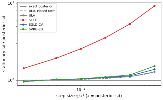
fig_12_S4. Download: PDF · SVG12.7.4 SG-HMC
p. 535, (12.128)–(12.132) One leapfrog step with stochastic gradients, \(\th_{t+1}=\th_t+\eta\bm v_t-\tfrac{\eta^2}{2}\bm g(\th_t,\xi_t)\) (12.131) and \(\bm v_{t+1}=\bm v_t-\tfrac\eta2\bm g(\th_t,\xi_t)-\tfrac\eta2\bm g(\th_{t+1},\xi_{t+1/2})\) (12.132). (In the second form of (12.129) the gradient coefficient should be \(\eta^2/2\), not \(\eta/2\): substitute (12.128) into the position update.) Zou and Gu (2021) bound its Wasserstein-2 error for strongly log-concave targets; the original SG-HMC of Chen, Fox and Guestrin (2014) adds friction to compensate the gradient noise, which leads to the next section.
12.7.5 Underdamped Langevin dynamics
pp. 535–536, (12.133) \(\d\th=\bm v\,\d t\), \(\d\bm v=-\bm g(\th)\d t-\gamma\bm v\,\d t+\sqrt{2\gamma}\,\d\bm W\) (12.133): Hamiltonian motion plus friction and matched noise.
Filling the gap 12.22: the invariant density of underdamped Langevin p. 536
Derivation
The Fokker–Planck equation of (12.133) for a density \(\rho(\th,\bm v)\) is \[ \partial_t\rho=-\bm v\cdot\nabla_{\th}\rho+\nabla E(\th)\cdot\nabla_{\bm v}\rho+\gamma\nabla_{\bm v}\cdot(\bm v\rho)+\gamma\Delta_{\bm v}\rho. \] Take \(\rho=e^{-E(\th)-\|\bm v\|^2/2}\), so \(\nabla_{\th}\rho=-\nabla E\,\rho\) and \(\nabla_{\bm v}\rho=-\bm v\rho\). The first two terms give \(\bm v\cdot\nabla E\,\rho-\nabla E\cdot\bm v\,\rho=0\) (the Hamiltonian part conserves \(e^{-H}\), as in Filling the gap 12.11). The last two give \(\gamma\nabla_{\bm v}\cdot(\bm v\rho+\nabla_{\bm v}\rho)=\gamma\nabla_{\bm v}\cdot(\bm v\rho-\bm v\rho)=0\) (friction and noise balance, an Ornstein–Uhlenbeck process in \(\bm v\) with stationary \(\N(\bm 0,\bm I)\)). So \(\rho\) is invariant and its \(\th\)-marginal is \(p\). The friction \(\gamma\) interpolates between Hamiltonian motion (\(\gamma\to0\)) and, after rescaling time, the overdamped Langevin diffusion (\(\gamma\to\infty\)). The second-order accuracy of its integrators claimed in the text is quoted from Leimkuhler, Matthews and Stoltz (2016).
12.8 Reversible jump (transdimensional) MCMC
p. 536 When the number of unknowns is itself unknown (the number of mixture components, of basis functions), the state space is a union \(\bigcup_m\{m\}\times\mathcal X_m\) of spaces of different dimensions. Green (1995) showed how to jump between them by matching dimensions with auxiliary variables.
12.8.1 Basic idea
pp. 536–537, (12.134)–(12.137), Figure 12.19 From \((n,\bm x_n)\), draw \(\bm u_{n,m}\sim q_{n\to m}\), map \((\bm x_m,\bm u_{m,n})=f_{n\to m}(\bm x_n,\bm u_{n,m})\) with a differentiable bijection, and accept with the ratio (12.136).
Filling the gap 12.23: Green's acceptance ratio from detailed balance pp. 536–537, (12.136)–(12.137)
Derivation
Let \(j(m\given n)\) be the probability of attempting a move from model \(n\) to \(m\) and require \(\dim\bm x_n+\dim\bm u_{n,m}=\dim\bm x_m+\dim\bm u_{m,n}\) (dimension matching). Detailed balance between the move \(n\to m\) and its reverse requires, for all measurable sets, \[ \int_{\{(\bm x_n,\bm u)\}}\pi(n,\bm x_n)j(m\given n)q_{n\to m}(\bm u)A_{n\to m}\,\d\bm x_n\d\bm u=\int_{\{(\bm x_m,\bm u')\}}\pi(m,\bm x_m)j(n\given m)q_{m\to n}(\bm u')A_{m\to n}\,\d\bm x_m\d\bm u', \] where the two regions correspond under \(f_{n\to m}\). Change variables on the right with \((\bm x_m,\bm u')=f_{n\to m}(\bm x_n,\bm u)\), \(\d\bm x_m\d\bm u'=|\det J|\,\d\bm x_n\d\bm u\), \(J=\partial f_{n\to m}/\partial(\bm x_n,\bm u)\). The equality then holds pointwise if \[ A_{n\to m}=\min\Big(1,\ \frac{\pi(m,\bm x_m)\,j(n\given m)\,q_{m\to n}(\bm u')}{\pi(n,\bm x_n)\,j(m\given n)\,q_{n\to m}(\bm u)}\,|\det J|\Big), \] by the same \(\min(a,b)\) symmetry as in Filling the gap 12.1, and \(A_{m\to n}\) is the minimum with the reciprocal ratio. The Jacobian is that of the forward map \((\bm x_n,\bm u)\mapsto(\bm x_m,\bm u')\), as used in (12.142); in (12.136)–(12.137) the subscripts of \(J\) are mixed up (the right side of (12.137) is the derivative of \(f_{n\to m}\) evaluated at \((\bm x_m,\bm u_{m,n})\)). When an auxiliary vector is empty its density is replaced by 1. The ratio compares densities on spaces of equal dimension, which resolves the "sphere against circle" problem of the text.
12.8.2 Example
pp. 537–539, (12.138)–(12.143), Figure 12.20, Algorithm 12.6 An RBF network \(f(x)=\sum_{j=1}^ka_j\phi(|x-\mu_j|)+\beta_1x+\beta_0\) (12.138) with Gaussian noise and an unknown number \(k\) of centres. Split moves \(\mu_{1,2}=\mu\mp u\beta\) (12.139) pair with merge moves to the midpoint (12.140); \(|\det J_{\text{split}}|=2\beta\) (12.142).
Algorithm 12.6 (generic reversible jump step) p. 539
With the current model \(k\), draw \(u\sim\Unif(0,1)\) and make a birth move if \(u\le b_k\), a death move if \(u\le b_k+d_k\), a split if \(u\le b_k+d_k+s_k\), a merge if \(u\le b_k+d_k+s_k+m_k\), and otherwise a fixed-dimension update. Here \(b_k=d_k=s_k=m_k=0.2\) where allowed (no birth or split at \(k_{\max}=6\), no death at 0, no split at 0, no merge below 2); updates are random-walk moves of one centre (rjmcmc_rbf).
Filling the gap 12.24: a complete reversible jump sampler for the RBF network, checked against quadrature pp. 537–539
The book gives the split and merge ratios schematically (with \(p(k,\mu_{k+1})\) in the denominator of (12.141) where \(p(k,\mu_k)\) is meant). Here is a sampler whose every factor is derived.
Derivation
Collapsing the coefficients. Let \(\bm D_k\) be the \(N\times(k+2)\) design with columns \(\phi(|x_i-\mu_j|)\), 1 and \(x_i\) (Gaussian bumps of fixed width 0.06). Put the \(g\)-prior \(\bm a\given\sigma^2\sim\N(\bm 0,\sigma^2\delta^2(\bm D^\T\bm D)^{-1})\) on the coefficients and \(\sigma^2\sim\mathrm{IG}(\nu_0/2,\gamma_0/2)\). Then \(\bm y\given\sigma^2\sim\N(\bm 0,\sigma^2(\bm I+\delta^2\bm H))\) with \(\bm H\) the hat matrix of \(\bm D\), a projection of rank \(m=k+2\). So \(\det(\bm I+\delta^2\bm H)=(1+\delta^2)^m\) and \((\bm I+\delta^2\bm H)^{-1}=\bm I-\tfrac{\delta^2}{1+\delta^2}\bm H\). Integrating \(\sigma^2\) against the inverse gamma gives \[ p(\bm y\given k,\bm\mu)=\frac{\Gamma(\tfrac{\nu_0+N}2)\,\gamma_0^{\nu_0/2}}{\Gamma(\tfrac{\nu_0}2)\,\pi^{N/2}}\,(1+\delta^2)^{-m/2}\big(\gamma_0+\bm y^\T\bm P\bm y\big)^{-(\nu_0+N)/2},\qquad\bm P=\bm I-\tfrac{\delta^2}{1+\delta^2}\bm H. \] Only the centres remain, so the dimension changes only in \(\bm\mu\) (this is the "collapsed" route the book's Section 12.8.3 recommends). Here \(\delta^2=20\), \(\nu_0=1\), \(\gamma_0=0.1\).
Priors and state. \(k\sim\) Poisson(1) truncated to \(\{0,\dots,6\}\); given \(k\), the centres are independent uniform on \(\Omega=[-0.1,1.1]\). The target is symmetric in the labels, so the state is stored as the sorted vector, whose density is \(k!/|\Omega|^k\).
Birth and death. Birth inserts a uniform new centre; death removes one of the \(k+1\) centres chosen uniformly. With \(\Lambda\) the likelihood ratio, \[ A_{\text{birth}}=\min\Big(1,\Lambda\,\frac{p(k+1)}{p(k)}\cdot\frac{(k+1)!/|\Omega|^{k+1}}{k!/|\Omega|^k}\cdot\frac{d_{k+1}/(k+1)}{b_k/|\Omega|}\Big)=\min\Big(1,\Lambda\,\frac{p(k+1)}{p(k)}\,\frac{d_{k+1}}{b_k}\Big): \] the uniform prior, the proposal density and the ordering factors cancel. No Jacobian (identity map).
Split and merge. Split picks one of \(k\) centres (\(s_k/k\)), draws \(u\sim\Unif(0,1)\) and maps \((\mu,u)\mapsto(\mu-u\beta,\mu+u\beta)\), \(\beta=0.1\), Jacobian \(2\beta\); it is rejected if a new centre leaves \(\Omega\) or another centre lies between the two. Merge picks one of the \(k\) adjacent pairs among \(k+1\) centres (\(m_{k+1}/k\)), requires their distance below \(2\beta\), and replaces them by the midpoint. The two moves are exact inverses, and \[ A_{\text{split}}=\min\Big(1,\Lambda\,\frac{p(k+1)}{p(k)}\cdot\frac{k+1}{|\Omega|}\cdot\frac{m_{k+1}}{s_k}\cdot2\beta\Big), \] with the factor \((k+1)/|\Omega|\) from the ratio of prior densities of the sorted vectors (no proposal density of a new centre cancels it here). The merge ratio is the reciprocal.
Check by quadrature. With \(k_{\max}=2\), \(p(k\given\bm y)\) can be computed exactly: \(Z_k=|\Omega|^{-k}\int_{\Omega^k}p(\bm y\given k,\bm\mu)\d\bm\mu\) on a \(241\)-point grid per centre. On a small noisy data set (25 points, noise sd 2.5) where the exact posterior spreads over \(k=0,1,2\), a run of \(6\times10^4\) iterations of the sampler with \(k_{\max}=2\) reproduces these probabilities to within 0.02. With \(k_{\max}=6\) and the data of Figure 12.20, the posterior is \(p(k=2)=0.67\), \(p(k=3)=0.28\), \(p(k=4)=0.05\), as in the book, where \(k=2\) also dominates.
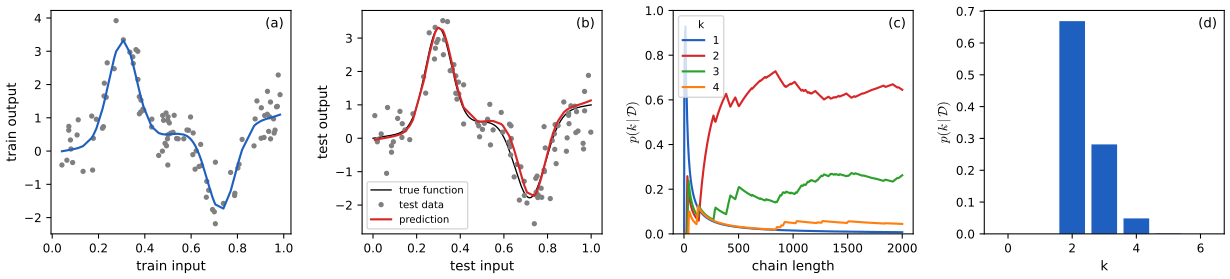
fig_12_20. Reproduces Murphy (2023), Figure 12.20. Download: PDF · SVG12.8.3 Discussion
p. 539 Reversible jump is fiddly mostly because of the continuous parameters that appear and disappear. Integrating them out, as above, leaves a sampler that changes only the structural variables. With fixed candidate centres the problem becomes discrete variable selection, where no Jacobian is needed at all. Bayesian nonparametric models (Chapter 31) avoid choosing \(k\) altogether.
12.9 Annealing methods
p. 539 A temperature parameter flattens a multimodal distribution so that a sampler can move between modes; cooling recovers the original.
12.9.1 Simulated annealing
pp. 540–542, (12.144)–(12.146), Figures 12.21–12.23 Sample \(p_T(\bm x)\propto\exp(-E(\bm x)/T)\) (12.144) with a Metropolis step at the current temperature, accepting with \(\exp(-(E(\bm x')-E(\bm x_t))/T_t)\) (12.146), while \(T_t\) decreases. The example is the "peaks" surface \(p(x,y)\propto|\mathrm{peaks}(x,y)|\) (12.145) on \([-3,3]^2\).
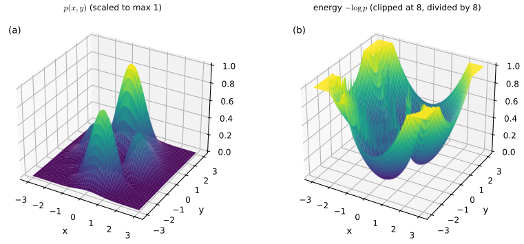
fig_12_21. Reproduces Murphy (2023), Figure 12.21. Download: PDF · SVG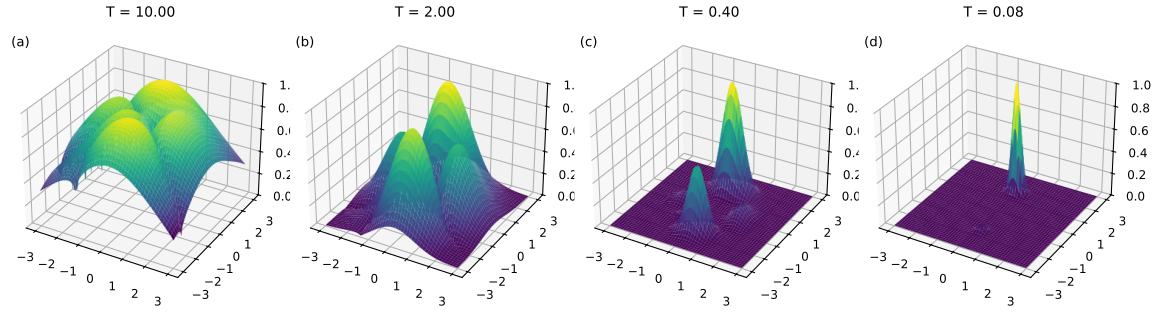
fig_12_22. Reproduces Murphy (2023), Figure 12.22. Download: PDF · SVG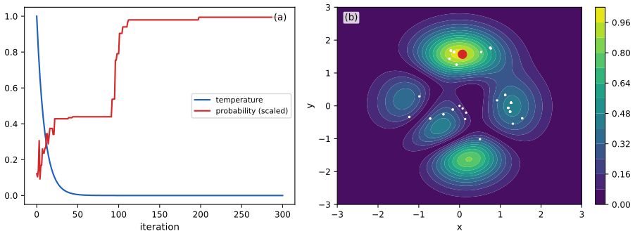
fig_12_23. Reproduces Murphy (2023), Figure 12.23. Download: PDF · SVGFilling the gap 12.25: why cooling finds the minimum, and the logarithmic schedule pp. 540–541
Derivation
Concentration. On a finite space with minimum energy \(E^*\) attained on \(\mathcal M\), \[ p_T(\bm x)=\frac{e^{-(E(\bm x)-E^*)/T}}{\sum_{\bm y}e^{-(E(\bm y)-E^*)/T}}\to\frac{\ind(\bm x\in\mathcal M)}{|\mathcal M|}\qquad(T\to0), \] since each term with \(E(\bm y)>E^*\) tends to 0 and each term in \(\mathcal M\) equals 1. On \(\R^D\), if \(E\) is continuous with a unique minimiser \(\bm x^*\) and \(\int e^{-E}<\infty\), then \(p_T\) converges weakly to \(\delta_{\bm x^*}\) (Laplace's principle): for any ball \(B\) around \(\bm x^*\), the mass outside \(B\) is at most \(e^{-(c_B-c'_B)/T}\) times a constant, where \(c_B\) is the minimum of \(E\) outside \(B\) and \(c'_B<c_B\) a value attained on a small neighbourhood of \(\bm x^*\).
The acceptance rule. (12.146) is the Metropolis ratio for \(p_{T_t}\) with a symmetric proposal, so at a fixed temperature the chain targets \(p_T\). Simulated annealing is a non-homogeneous chain: it converges to \(\mathcal M\) only if the temperature falls slowly enough for the chain to keep up. Hajek (1988) proved that \(T_t=c/\log(t+1)\) gives convergence in probability to \(\mathcal M\) if and only if \(c\) is at least the depth of the deepest local minimum that is not global (the energy barrier that must be climbed to leave it); the proof is not reproduced here. Geometric cooling \(T_{t+1}=\gamma T_t\) is far faster and carries no guarantee, which the success rates in Figure 12.23 illustrate.
12.9.2 Parallel tempering
p. 542 Run chains at temperatures \(1=T_1<T_2<\dots\) in parallel and occasionally propose to swap the states of neighbouring chains; hot chains cross barriers and pass good states down to the cold chain, whose draws target \(p\).
Filling the gap 12.26: the swap acceptance probability p. 542
Derivation
The joint target of the replicas is \(\prod_kp_{\beta_k}(\bm x_k)\) with \(\beta_k=1/T_k\) and \(p_\beta\propto e^{-\beta E}\); each replica's own MCMC moves leave it invariant. Swapping \(\bm x_i\leftrightarrow\bm x_j\) is a symmetric deterministic proposal, so the MH ratio is \[ \frac{p_{\beta_i}(\bm x_j)\,p_{\beta_j}(\bm x_i)}{p_{\beta_i}(\bm x_i)\,p_{\beta_j}(\bm x_j)}=\exp\big((\beta_i-\beta_j)(E(\bm x_i)-E(\bm x_j))\big), \] in which the unknown normalising constants cancel. A swap that hands the lower energy to the colder chain is always accepted. The marginal of the \(T=1\) replica is \(p\) exactly, and only its draws are used. Neighbouring temperatures must be close enough that the energy distributions overlap, otherwise swaps are rarely accepted.
Practice problems
Chapter 12 of the book has no end-of-chapter exercises. Here are three short problems with worked solutions.
Problem 12.1 (the independence sampler converges geometrically). Let \(w=p^*/q\le M\) everywhere. Show that the independence-sampler kernel satisfies \(K(\bm x,\d\bm y)\ge p^*(\bm y)\d\bm y/M\) for every \(\bm x\), and deduce \(\|K^t(\bm x,\cdot)-p^*\|_\TV\le(1-1/M)^t\).
Solution
The moving part of the kernel has density \(q(\bm y)\min(1,w(\bm y)/w(\bm x))\). Since \(w(\bm x)\le M\) and \(w(\bm y)/M\le1\), \[ \min\Big(1,\frac{w(\bm y)}{w(\bm x)}\Big)\ge\min\Big(1,\frac{w(\bm y)}{M}\Big)=\frac{w(\bm y)}{M}, \] hence \[ K(\bm x,\d\bm y)\ge\frac{q(\bm y)w(\bm y)}{M}\d\bm y=\frac{p^*(\bm y)}{M}\d\bm y, \] a Doeblin minorisation with constant \(\varepsilon=1/M\). Write \(K=\varepsilon p^*+(1-\varepsilon)R\) with \(R\) a Markov kernel. Then \(K^t(\bm x,\cdot)-p^*=(1-\varepsilon)^t\big(R'_t(\bm x,\cdot)-p^*\big)\) for a probability kernel \(R'_t\): by induction, using \(p^*K=p^*\), \(\mu K-p^*=(1-\varepsilon)(\mu R-p^*R)\) for any probability \(\mu\), and the total variation distance between two probabilities is at most 1. So \(\|K^t(\bm x,\cdot)-p^*\|_\TV\le(1-1/M)^t\). Example: \(p^*=\N(0,1)\), \(q=\N(0,2^2)\) gives \(w(x)=2e^{-3x^2/8}\le2\), so the distance at least halves at every step. The bound was confirmed exactly on a discretised version of this example (powers of the kernel matrix).
Problem 12.2 (Barker against Metropolis). Barker's rule accepts with \(p^*(\bm x')/(p^*(\bm x)+p^*(\bm x'))\) for a symmetric proposal. (a) Show that it also satisfies detailed balance. (b) On two states with \(p^*=(p,1-p)\), \(p<\tfrac12\), always propose the other state. Find the second eigenvalue of each chain and the asymptotic variance of the average of \(f=\ind(\text{state }2)\). Which sampler is better?
Solution
(a) \(p^*(\bm x)q(\bm x'\given\bm x)\frac{p^*(\bm x')}{p^*(\bm x)+p^*(\bm x')}\) is symmetric in \(\bm x,\bm x'\) when \(q\) is.
(b) Metropolis: \(P_{12}=\min(1,(1-p)/p)=1\), \(P_{21}=p/(1-p)\), second eigenvalue \(\lambda=1-P_{12}-P_{21}=-p/(1-p)\). Barker: \(P_{12}=1-p\), \(P_{21}=p\), \(\lambda=0\): Barker's chain produces independent draws. For a two-state chain the autocorrelation of \(f\) is \(\lambda^\ell\), so the asymptotic variance of \(\bar f\) is \(\tfrac{\sigma_f^2}{N}\cdot\frac{1+\lambda}{1-\lambda}\) with \(\sigma_f^2=p(1-p)\). For Metropolis \(\frac{1+\lambda}{1-\lambda}=\frac{1-2p}{1}=1-2p<1\); for Barker it is 1. Metropolis wins: its negative correlation makes its average better than independent sampling (for \(p=0.2\), variance factor 0.6). This is Peskun's (1973) theorem in miniature: Metropolis has the larger off-diagonal transition probabilities, hence the smaller asymptotic variance for every \(f\). Simulations of \(10^5\) steps with \(p=0.2\) give variance factors 0.60 and 1.00.
Problem 12.3 (systematic-scan Gibbs is not reversible). For Gibbs sampling of \(\N(\bm 0,[[1,\rho],[\rho,1]])\), compute the lag-one cross-covariance matrix \(\bm C=\cov(\bm x_t,\bm x_{t+1})\) under stationarity for the systematic scan (update \(x_1\), then \(x_2\)). Show that \(\bm C\) is not symmetric, and explain why that proves the chain is not reversible. What changes for the random scan?
Solution
With \(\bm x_t=(x_1,x_2)\), \(x_1'=\rho x_2+s\varepsilon_1\) and \(x_2'=\rho x_1'+s\varepsilon_2\). Then \(\cov(x_1,x_1')=\rho\cov(x_1,x_2)=\rho^2\), \(\cov(x_1,x_2')=\rho\cdot\rho^2=\rho^3\), \(\cov(x_2,x_1')=\rho\), \(\cov(x_2,x_2')=\rho^2\): \[ \bm C=\begin{pmatrix}\rho^2&\rho^3\\\rho&\rho^2\end{pmatrix}. \] If the chain were reversible, \((\bm x_t,\bm x_{t+1})\) and \((\bm x_{t+1},\bm x_t)\) would have the same distribution, so \(\bm C=\cov(\bm x_{t+1},\bm x_t)=\bm C^\T\). But \(\rho^3\ne\rho\) unless \(\rho\in\{0,\pm1\}\). For the random scan (update \(x_1\) or \(x_2\) with probability \(\tfrac12\) each) the kernel is a mixture of two reversible kernels, hence reversible (Filling the gap 12.3); its cross-covariance is \(\tfrac12\begin{pmatrix}\rho^2&\rho\\\rho&1\end{pmatrix}+\tfrac12\begin{pmatrix}1&\rho\\\rho&\rho^2\end{pmatrix}\), symmetric. A simulation of \(2\times10^5\) sweeps with \(\rho=0.8\) gives the off-diagonal entries 0.512 and 0.800 for the systematic scan, matching \(\rho^3\) and \(\rho\).
Demonstrations for this chapter
Each demonstration runs in the browser, with seeded random numbers so that a class sees the same pictures, and links back to these notes. The ▶ Demo boxes above open them already set to the case under discussion. The pages run the same algorithms as the Python code, with the same random-number generator, so their numbers are those of the code.
| Demonstration | What you can see | Sections and results |
|---|---|---|
| Metropolis-Hastings proposals and diagnostics | Four random walk Metropolis or Gibbs chains on the two-mode mixture: traces, histogram, autocorrelation, R-hat and effective sample size as the proposal scale changes. Presets: 1 tau = 1; 2 tau = 500; 3 tau = 8; 4 Gibbs; 5 tau = 60. | 12.2.3, 12.3.5, 12.6.2, 12.6.3; Filling the gaps 12.2, 12.5, 12.18 |
| Hamiltonian Monte Carlo | HMC or random walk Metropolis on a correlated Gaussian, the funnel in both parameterisations and the car posterior, with the last leapfrog trajectory, divergences and effective sample sizes. Presets: 1 tuned; 2 unstable step; 3 MALA; 4 random walk; 5 funnel centred; 6 funnel non-centred; 7 cars. | 12.5, 12.6.5; Filling the gaps 12.12, 12.14, 12.20 |
| Gibbs against Swendsen-Wang | Two Ising lattices sampled side by side, with magnetisation traces and Onsager's exact value. Presets: 1 J = 0.3; 2 critical; 3 J = 0.6 from all +1; 4 J = 0.6 random start; 5 J = 1. | 12.3.3, 12.4.2; Filling the gaps 12.4, 12.10 |
The Python code that produces every figure of this page is code/ch12_mcmc.py (see the code index).
Errors and slips found in the book
Everything below was confirmed by recomputation or by the derivations above. Items marked (minor) are notational.
- (12.56): the collapsed-Gibbs prior predictive should be \((N_{k,-i}+\alpha/K)/(N+\alpha-1)\), not \((N_{k,-i}+\alpha)/(N+\alpha-1)\); the middle of (12.56) and Algorithm 12.2 have \(\alpha/K\) (Filling the gap 12.8).
- (12.115): with \(x\sim\N(0,\exp(\nu))\) (variance), the non-centred form is \(x=z\exp(\nu/2)\), not \(z\exp(\nu)\) (Filling the gap 12.20).
- (12.75) and Section 12.5.4.3: with \(K=\tfrac12\bm v^\T\bm\Sigma^{-1}\bm v\) (12.64), \(\bm\Sigma\) is the mass matrix; (12.75) and the text after Algorithm 12.3 write \(\tfrac12\bm v^\T\bm\Sigma\bm v\), and Section 12.5.4.3 calls \(\bm\Sigma\) the inverse mass while setting it to the posterior covariance. The posterior covariance belongs in the inverse mass (Filling the gap 12.13). (12.80) has the same issue.
- (12.84) with (12.88): the loss must be the average, not the sum, for the minibatch gradient (12.85) to be unbiased (Filling the gap 12.15).
- (12.96) and the eigengap of Section 12.6.1: the conductance numerator needs the weights \(p^*(\bm x)\) and the minimum should exclude \(p^*(S)=0\); the mixing bound needs the absolute spectral gap \(1-\max(|\lambda_2|,|\lambda_n|)\), not \(\lambda_1-\lambda_2\) (the walk of Figure 12.11 has \(\lambda_{21}=-0.989\)) (Filling the gap 12.17).
- (12.129): the second form of the position update should have \(\tfrac{\eta^2}{2}\nabla E(\th_t)\), not \(\tfrac\eta2\nabla E(\th_t)\); (12.131) is right.
- (12.136)–(12.137) and (12.141): the Jacobian in Green's ratio is that of the forward map \(f_{n\to m}\) at \((\bm x_n,\bm u_{n,m})\) (Filling the gap 12.23); in (12.141) the denominator should be \(p(k,\bm\mu_k)\).
- Section 12.4.2: the Gibbs step \(p(\bm x\given\bm v)\) gives every cluster an independent random spin; the text's "pick one component" is a valid but different (slower) move (Filling the gap 12.10).
- (minor) (12.25): \(\psi(x_i=-1,x_i)\) should be \(\psi(x_i=-1,x_j)\). After (12.7): \(p^*\) is invariant for the MH kernel, not for the proposal \(q\). (12.69): uses \(\bm v_{t+1}\), which is the modified Euler update rather than (12.68). Algorithm 12.5, line 5: \(\tilde g=\sum_n\nabla E_n(\tilde\th)\) (the \(\nabla\) is missing). Theorem 12.2.1: "ergodic and irreducible" is redundant.
References
- Murphy, K. P. (2023). Probabilistic Machine Learning: Advanced Topics. MIT Press. Chapter 12 (pp. 499–542). probml.github.io/pml-book/book2.html.
- Andrieu, C. and Thoms, J. (2008). A tutorial on adaptive MCMC. Statistics and Computing, 18, 343–373.
- Chen, T., Fox, E. and Guestrin, C. (2014). Stochastic gradient Hamiltonian Monte Carlo. ICML.
- Duane, S., Kennedy, A. D., Pendleton, B. J. and Roweth, D. (1987). Hybrid Monte Carlo. Physics Letters B, 195, 216–222.
- Gelfand, A. E. and Smith, A. F. M. (1990). Sampling-based approaches to calculating marginal densities. Journal of the American Statistical Association, 85, 398–409.
- Geman, S. and Geman, D. (1984). Stochastic relaxation, Gibbs distributions, and the Bayesian restoration of images. IEEE Transactions on Pattern Analysis and Machine Intelligence, 6, 721–741.
- Geyer, C. J. (1992). Practical Markov chain Monte Carlo. Statistical Science, 7, 473–483.
- Green, P. J. (1995). Reversible jump Markov chain Monte Carlo computation and Bayesian model determination. Biometrika, 82, 711–732.
- Hajek, B. (1988). Cooling schedules for optimal annealing. Mathematics of Operations Research, 13, 311–329.
- Hastings, W. K. (1970). Monte Carlo sampling methods using Markov chains and their applications. Biometrika, 57, 97–109.
- Hoffman, M. D. and Gelman, A. (2014). The no-U-turn sampler. Journal of Machine Learning Research, 15, 1593–1623.
- Jerrum, M. and Sinclair, A. (1989). Approximating the permanent. SIAM Journal on Computing, 18, 1149–1178.
- Lawler, G. F. and Sokal, A. D. (1988). Bounds on the \(L^2\) spectrum for Markov chains and Markov processes: a generalization of Cheeger's inequality. Transactions of the American Mathematical Society, 309, 557–580.
- Leimkuhler, B., Matthews, C. and Stoltz, G. (2016). The computation of averages from equilibrium and nonequilibrium Langevin molecular dynamics. IMA Journal of Numerical Analysis, 36, 13–79.
- Li, Q., Tai, C. and E, W. (2017). Stochastic modified equations and adaptive stochastic gradient algorithms. ICML.
- Ma, Y.-A., Chen, T. and Fox, E. (2015). A complete recipe for stochastic gradient MCMC. NeurIPS.
- Metropolis, N., Rosenbluth, A. W., Rosenbluth, M. N., Teller, A. H. and Teller, E. (1953). Equation of state calculations by fast computing machines. Journal of Chemical Physics, 21, 1087–1092.
- Neal, R. M. (2003). Slice sampling. Annals of Statistics, 31, 705–767.
- Neal, R. M. (2011). MCMC using Hamiltonian dynamics. In Handbook of Markov Chain Monte Carlo, Chapman and Hall/CRC.
- Peskun, P. H. (1973). Optimum Monte-Carlo sampling using Markov chains. Biometrika, 60, 607–612.
- Roberts, G. O., Gelman, A. and Gilks, W. R. (1997). Weak convergence and optimal scaling of random walk Metropolis algorithms. Annals of Applied Probability, 7, 110–120.
- Roberts, G. O. and Rosenthal, J. S. (2001). Optimal scaling for various Metropolis-Hastings algorithms. Statistical Science, 16, 351–367.
- Roberts, G. O. and Rosenthal, J. S. (2007). Coupling and ergodicity of adaptive Markov chain Monte Carlo algorithms. Journal of Applied Probability, 44, 458–475.
- Swendsen, R. H. and Wang, J.-S. (1987). Nonuniversal critical dynamics in Monte Carlo simulations. Physical Review Letters, 58, 86–88.
- Tierney, L. (1994). Markov chains for exploring posterior distributions. Annals of Statistics, 22, 1701–1728.
- Vehtari, A., Gelman, A., Simpson, D., Carpenter, B. and Bürkner, P.-C. (2021). Rank-normalization, folding, and localization: an improved R-hat for assessing convergence of MCMC. Bayesian Analysis, 16, 667–718.
- Welling, M. and Teh, Y. W. (2011). Bayesian learning via stochastic gradient Langevin dynamics. ICML.
- Zou, D. and Gu, Q. (2021). On the convergence of Hamiltonian Monte Carlo with stochastic gradients. ICML.
The numerical statements in the text (acceptance rates, exact autocorrelations, transition probabilities and eigenvalues, the collapsed-Gibbs ratio, leapfrog stability and the modified energy, the MALA identity, the ULA variance, the minibatch moments, R-hat and effective sample sizes, the reversible jump posterior against quadrature, and the practice problems) were confirmed numerically.