Nonparametric Bayesian models
A Bayesian nonparametric model puts its prior directly on an infinite-dimensional object: a function, a probability distribution, a partition of the data into an unbounded number of clusters, a binary matrix with unboundedly many columns, or a random set of points. The book's chapter is a two-page pointer; the substance is in the supplement, which these notes follow section by section: the Dirichlet process and its three faces (finite-dimensional Dirichlet marginals, stick breaking, the Chinese restaurant), Dirichlet process mixtures fitted by collapsed Gibbs sampling, variational inference and the DP-means limit, the Pitman-Yor and hierarchical processes, the Indian buffet and beta processes, completely random measures and Lévy processes, and point processes that repel or reinforce (Poisson, renewal, Hawkes, Gibbs and determinantal). Every result the supplement states without proof is derived below, and several of its formulas are corrected.
Ch. 1 Introduction Ch. 2 Probability Ch. 3 Statistics Ch. 4 Graphical models Ch. 5 Information theory Ch. 6 Optimisation Ch. 7 Inference algorithms Ch. 8 Gaussian filtering Ch. 9 Message passing Ch. 10 Variational inference Ch. 11 Monte Carlo Ch. 12 MCMC Ch. 13 Sequential Monte Carlo Ch. 14 Predictive models Ch. 15 GLMs Ch. 16 Deep networks Ch. 17 Bayesian neural networks Ch. 18 Gaussian processes Ch. 19 Beyond iid Ch. 20 Generative models Ch. 21 VAEs Ch. 22 Autoregressive models Ch. 23 Normalizing flows Ch. 24 Energy-based models Ch. 25 Diffusion models Ch. 26 GANs Ch. 27 Discovery methods Ch. 28 Latent factor models Ch. 29 State-space models Ch. 30 Graph learning Ch. 31 Nonparametric Bayes Ch. 32 Representation learning Ch. 33 Interpretability Ch. 34 Decision making Ch. 35 Reinforcement learning Ch. 36 Causality
How to read these notes
They follow the book. The printed chapter has a single section, 31.1; everything else is in the online supplement, whose sections are numbered 31.1 to 31.8 again. To avoid the clash, supplement sections are written S31.k and labelled supplement, supplement equations S(31.n) and supplement figures S31.k. Equations without a number are steps the book skips.
Filling the gaps. Wherever the supplement writes "one can show", "it is easy to see", quotes a result from the literature, or leaves a step to the reader, an orange Filling the gap box gives the full argument. Proofs start hidden: open one with its bar, or use the buttons below. Results already proved on this site are stated and linked rather than repeated: the Dirichlet process definition, its posterior and its consistency are in Nonparametric Statistical Inference, gap 10.9; the Dirichlet distribution and its gamma construction in gap 2.6 of this course; the normal-inverse-Wishart predictive in gap 3.10; coordinate-ascent variational inference in gap 10.11; collapsed Gibbs for finite mixtures in Algorithm 12.2; k-means as the small-variance limit of EM in Volume 1, gap 21.5.
Figures and demonstrations. Every computed figure of the supplement is reproduced by the Python code, written from scratch (the samplers, the variational updates, DP-means, the point-process simulators and the DPP sampler are implemented by hand). Figures S31.3(a), S31.5 and S31.13 are diagrams. The data of Figure S31.6 are not given in the book, and the Swedish pines and California redwoods of Figure S31.11 are not available, so those figures use simulated stand-ins, as their captions say. Four figures of my own (marked x) illustrate results the supplement only states.
Main reference
K. P. Murphy, Probabilistic Machine Learning: Advanced Topics, MIT Press (2023; online draft of December 2025), Chapter 31, pages 1081–1082 (book page: probml.github.io/pml-book/book2.html), and the supplementary material, Chapter 31, pages 267–300 (the chapter is written by Vinayak Rao, Section S31.2.3 by Xinglong Li). Section, equation, figure and algorithm numbers below refer to this book. The explanations, derivations, figures and code are my own. The chapter has no exercises; three practice problems are given instead.
Companion courses
The Dirichlet process is introduced, with its posterior and consistency, in Nonparametric Statistical Inference, Section 10.3 (gap 10.9), so these notes start from there and spend their derivations on what the supplement adds. Gaussian processes, the other basic nonparametric prior mentioned in Section 31.1, are Chapter 18 of this course. Finite mixtures, EM and k-means are in Volume 1, Chapter 21; collapsed Gibbs for a finite mixture in Chapter 12; mean-field variational inference in Chapter 10; topic models (which the hierarchical Dirichlet process makes nonparametric) in Chapter 28.
What this chapter adds: the stick-breaking theorem with a proof, the correct Ewens formula and the exact law of the number of clusters, the growth \(K_N/\log N\to\alpha\), the collapsed Gibbs conditionals, the variational updates of Algorithm S31.2, the Escobar–West update for \(\alpha\), the small-variance limit behind DP-means, the Pitman-Yor and Gibbs-type partition laws, the coagulation identity, the IBP's Poisson laws, the Poisson construction of completely random measures and the gamma-Dirichlet link, the thinning theorem, the Hawkes likelihood and its moments, and the algebra of determinantal point processes.
The chapter at a glance
- S31.1 The DP, its posterior and predictive (gap 31.1); stick breaking (31.2); the CRP, the Ewens formula and the number of tables (31.3).
- S31.2 Finite mixtures converge to the DP mixture (gap 31.4); the collapsed Gibbs conditionals (31.5); variational updates (31.6); the posterior of \(\alpha\) (31.7).
- S31.3 Pitman-Yor: partitions, growth, coagulation; Gibbs-type priors (gap 31.8); the HDP shares atoms (31.9).
- S31.4 The IBP's Poisson laws and the beta process (gap 31.10). S31.5 DP-means (gap 31.11).
- S31.6–S31.7 CRMs, the gamma process and the DP (gap 31.12); infinite divisibility (31.13).
- S31.8 Poisson processes and thinning (gap 31.14); renewal processes (31.15); the Hawkes likelihood and moments (31.16); Gibbs processes (31.17); DPPs (31.18).
Notation. \(\Theta\) is the parameter space, \(H\) a probability measure on it (the base measure), \(\alpha\gt0\) a concentration. A random measure is \(G=\sum_k\pi_k\delta_{\theta_k}\). \(N\) is the number of observations, \(K\) (or \(K_N\)) the number of occupied clusters, \(N_k\) the size of cluster \(k\). \((x)_n=x(x+1)\cdots(x+n-1)\) is the rising factorial, \((x)_0=1\). \(\ind(\cdot)\) is an indicator.
Prerequisites. Chapters 2, 3, 10 and 12 of the book; the Dirichlet process box in the nonparametric statistics course.
31.1 Introduction
p. 1081 A parametric model indexes its objects (regression functions, densities, graphs) by a fixed finite-dimensional vector, and a Bayesian puts the prior on that vector. A Bayesian nonparametric (BNP) model puts the prior on the object itself, through a stochastic process: a law on a possibly infinite collection of random variables, specified by its finite-dimensional marginals. The Gaussian process of Chapter 18 is the prototype: \(f(\bm X)=(f(\bm x_1),\dots,f(\bm x_N))\sim\N(\bm\mu(\bm X),\bm K(\bm X))\) for every finite set of inputs, with Gram matrix \([\bm K(\bm X)]_{ij}=K(\bm x_i,\bm x_j)\). Two features make such models useful. The posterior can become as complex as the data demand (no underfitting), while averaging over the infinitely many unknowns guards against overfitting; and inference and prediction only ever touch the finitely many variables attached to training and test points, which is why they are tractable. The rest of the chapter applies the same idea to random probability measures, partitions, feature allocations and point patterns.
See also. Chapter 18 (Gaussian processes), Nonparametric Statistical Inference, Section 10.3.
S31.1 Dirichlet processes supplement
S31.1.1 Definition of a DP
Supp. pp. 267–269, S(31.1)–S(31.7) A random probability measure \(G\) on \(\Theta\) is a Dirichlet process, \(G\sim\DP(\alpha,H)\) (Ferguson 1973), if for every finite measurable partition \((T_1,\dots,T_K)\) of \(\Theta\)
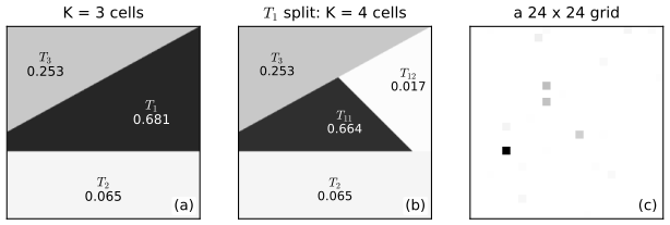
\[ (G(T_1),\dots,G(T_K))\sim\Dir\big(\alpha H(T_1),\dots,\alpha H(T_K)\big). \tag{S31.1} \]These laws are consistent under merging cells (the aggregation property of the Dirichlet), so Kolmogorov's extension theorem gives a process; then \(\E G(T)=H(T)\) and \(\var G(T)=H(T)(1-H(T))/(1+\alpha)\): \(H\) is the prior guess and \(\alpha\) its prior sample size. All of this, and the posterior below for a partition, is proved in Nonparametric Statistical Inference, gap 10.9. Figure S31.1 shows one draw of \(G\) seen through two nested partitions and a fine grid: the masses on the refined partition add up to those on the coarse one, which is the consistency property in action.
Conjugacy. If \(\theta_1,\dots,\theta_N\given G\) are iid \(G\), the counts in the cells of a partition are multinomial, and Dirichlet–multinomial conjugacy gives \((G(T_1),\dots,G(T_K))\given\theta_{1:N}\sim\Dir\big(\alpha H(T_1)+n_1,\dots,\alpha H(T_K)+n_K\big)\) with \(n_k=\sum_i\ind(\theta_i\in T_k)\) (S31.6), so
\[ G\given\theta_{1:N},\alpha,H\sim\DP\Big(\alpha+N,\ \frac{1}{\alpha+N}\Big(\alpha H+\sum_{i=1}^N\delta_{\theta_i}\Big)\Big). \tag{S31.7} \](The supplement prints \(G(T_k)\) where \(\alpha H(T_k)\) belongs in S(31.6); see the notes on the book.) The posterior base measure is a convex combination of the prior guess and the empirical distribution with weight \(N/(\alpha+N)\to1\) on the data, and the concentration \(\alpha+N\) grows, so the posterior concentrates at the empirical distribution.
Filling the gap 31.1: the predictive distribution, and why the posterior statement holds for all partitions at once Supp. pp. 269–271, S(31.7), S(31.12)–S(31.13)
Derivation
(i) The first draw. For any measurable \(T\), \(\Pr(\theta_1\in T)=\E[\Pr(\theta_1\in T\given G)]=\E G(T)=H(T)\) by the mean of the Beta marginal \(\Betad(\alpha H(T),\alpha(1-H(T)))\). As this holds for every \(T\), \(\theta_1\sim H\) (S31.12).
(ii) The next draw. By (S31.7) applied to \(\theta_{1:N}\), \(G\given\theta_{1:N}\) is a DP with base measure \(\bar H_N=(\alpha H+\sum_i\delta_{\theta_i})/(\alpha+N)\); repeating (i) with this DP,
\[ \Pr(\theta_{N+1}\in T\given\theta_{1:N})=\bar H_N(T)=\frac{\alpha H(T)+\sum_{k=1}^KN_k\ind(\theta^*_k\in T)}{\alpha+N}, \]where \(\theta^*_1,\dots,\theta^*_K\) are the distinct values among \(\theta_{1:N}\) and \(N_k\) their multiplicities. This is (S31.13): with probability \(N_k/(\alpha+N)\) repeat an old value, with probability \(\alpha/(\alpha+N)\) draw a fresh one from \(H\) (which, if \(H\) has no atoms, is new with probability one). This is the Blackwell–MacQueen urn.
(iii) The book's "it is easy to see". The step from "the posterior of every partition's cell probabilities is the corresponding Dirichlet" to "the posterior of \(G\) is a DP" needs care, because S(31.6) conditions only on the counts \(n_k\), not on the exact values \(\theta_i\). The clean argument goes through the predictive: the joint law of \((G,\theta_{1:N})\) is determined by the law of \(\theta_{1:N}\) (the urn of (ii), which follows from (i) and Bayes' rule on any partition fine enough to separate the \(\theta_i\)) together with the conditional law of \(G\); and one checks that the pair "\(\theta_{1:N}\) from the urn, then \(G\sim\DP(\alpha+N,\bar H_N)\)" has the same finite-dimensional joint laws \((G(T_1),\dots,G(T_K),\theta_{1:N})\) as "\(G\sim\DP(\alpha,H)\), then \(\theta_i\) iid \(G\)" for every partition, by the partition computation. Ferguson (1973, Theorem 1) gives the details; the nonparametric statistics notes give the partition step.
The predictive is confirmed numerically by importance-weighting draws of \(G(T)\) from its Beta prior with the likelihood of the counts: the weighted mean matches \((\alpha H(T)+n_T)/(\alpha+N)\). ∎
S31.1.2 Stick breaking construction of the DP
Supp. pp. 269–270, S(31.8)–S(31.11) A draw from a DP is discrete with probability one, \(G=\sum_{k\ge1}\pi_k\delta_{\theta_k}\) (S31.8). Sethuraman (1994) gives the weights and atoms explicitly: for \(k=1,2,\dots\)
\[ \beta_k\sim\Betad(1,\alpha),\qquad\theta_k\sim H,\qquad \pi_k=\beta_k\prod_{l=1}^{k-1}(1-\beta_l)=\beta_k\Big(1-\sum_{l=1}^{k-1}\pi_l\Big), \tag{S31.9–S31.10} \]all independent; the law of \(\bm\pi\) is written \(\GEM(\alpha)\) (S31.11). Break a fraction \(\beta_1\) off a stick of length one, then a fraction \(\beta_2\) of what is left, and so on. Small \(\alpha\) makes the first few pieces large; large \(\alpha\) spreads the mass over many small pieces (Figure S31.3).
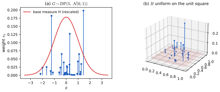
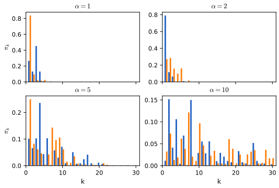
Filling the gap 31.2: the weights sum to one, how fast, and why the stick-breaking measure is a DP Supp. p. 270, "one can show that \(G\sim\DP(\alpha,H)\)"
Proof
(i) The weights sum to one almost surely, geometrically fast in mean. By induction on (S31.10), the mass not yet allocated after \(K\) breaks is \(R_K=1-\sum_{k\le K}\pi_k=\prod_{k\le K}(1-\beta_k)\). The \(\beta_k\) are independent with \(\E(1-\beta_k)=\alpha/(1+\alpha)\), so \(\E R_K=(\alpha/(1+\alpha))^K\to0\). \(R_K\) is non-increasing and non-negative, so it has an almost-sure limit \(R_\infty\ge0\), and \(\E R_\infty\le\E R_K\to0\) forces \(R_\infty=0\) a.s. In particular \(\E\pi_k=\E R_{k-1}\E\beta_k=\alpha^{k-1}/(1+\alpha)^k\): the weights decrease in mean (they are "stochastically ordered" only in this sense; individual draws need not be decreasing, see Figure S31.3). The truncation error after \(K\) atoms is \((\alpha/(1+\alpha))^K\) in mean, which is why truncating at a few times \(\alpha\log(1/\epsilon)\) atoms is harmless.
(ii) A distributional equation. Write \(G=\beta_1\delta_{\theta_1}+(1-\beta_1)G'\), where \(G'=\sum_{k\ge2}(\pi_k/(1-\beta_1))\delta_{\theta_k}\) is built from \((\beta_2,\beta_3,\dots)\) and \((\theta_2,\dots)\) exactly as \(G\) is built from the full sequences, so \(G'\) has the same law as \(G\) and is independent of \((\beta_1,\theta_1)\). We show the DP satisfies the same equation and that the equation has a unique solution.
(iii) The DP satisfies it. Fix a partition with \(a_j=\alpha H(T_j)\), \(\sum_ja_j=\alpha\). Let \(\bm P\sim\Dir(\bm a)\), \(\beta\sim\Betad(1,\alpha)\), \(\theta\sim H\) independent, and \(J\) the cell containing \(\theta\), so \(\Pr(J=j)=a_j/\alpha\). Use the gamma construction (gap 2.6): \(g_j\sim\Ga(a_j,1)\), \(g_0\sim\Ga(1,1)\) independent, \(\bm P=\bm g/\sum g\) and \(\beta=g_0/(g_0+\sum g)\) independent of \(\bm P\) (the total \(\sum g\sim\Ga(\alpha,1)\) is independent of \(\bm P\)). Then \(\beta\bm e_j+(1-\beta)\bm P=(\bm g+g_0\bm e_j)/(g_0+\sum g)\), and \(g_j+g_0\sim\Ga(a_j+1,1)\), so given \(J=j\) the vector is \(\Dir(\bm a+\bm e_j)\). Mixing over \(J\), with \(\Dir(\bm p\given\bm a+\bm e_j)=(\alpha/a_j)\,p_j\Dir(\bm p\given\bm a)\),
\[ \sum_j\frac{a_j}{\alpha}\Dir(\bm p\given\bm a+\bm e_j)=\sum_jp_j\Dir(\bm p\given\bm a)=\Dir(\bm p\given\bm a). \]So if \(G'\sim\DP(\alpha,H)\), then \(\beta\delta_\theta+(1-\beta)G'\) has the right Dirichlet marginals on every partition: it is \(\DP(\alpha,H)\).
(iv) Uniqueness. Let \(G\) and \(\tilde G\) both solve the equation in law. Couple them: iterate the map \(m\) times with the same \((\beta_k,\theta_k)_{k\le m}\), starting from independent copies \(G^{(m)},\tilde G^{(m)}\). The results have the laws of \(G\) and \(\tilde G\), and for every set \(T\), \(|G(T)-\tilde G(T)|\le\prod_{k\le m}(1-\beta_k)=R_m\to0\) a.s. Hence the finite-dimensional laws agree and \(G\overset{d}{=}\tilde G\). The stick-breaking measure solves the equation by (ii), the DP by (iii), so they coincide. Discreteness of the DP follows. ∎
The weight means, the truncation error and the moments \(\E G(T)=H(T)\), \(\var G(T)=H(T)(1-H(T))/(1+\alpha)\) are confirmed numerically by simulating truncated stick breaking.
S31.1.3 The Chinese restaurant process (CRP)
Supp. pp. 271–272, S(31.12)–S(31.15) Integrating \(G\) out turns the iid sample into the urn of gap 31.1. Keeping only the labels \(z_i\) (which cluster \(\theta_i\) belongs to, numbered in order of appearance) gives the Chinese restaurant process: with \(K\) occupied tables among \(N\) customers,
\[ p(z_{N+1}=z\given z_{1:N},\alpha)=\frac{1}{\alpha+N}\Big(\alpha\,\ind(z=K+1)+\sum_{k=1}^KN_k\ind(z=k)\Big). \tag{S31.14} \]Customers join a table in proportion to its size (rich get richer) or open a new one in proportion to \(\alpha\); each table serves a dish \(\theta^*_k\sim H\). The labels separate the clustering (governed by \(\alpha\)) from the cluster parameters (governed by \(H\)). The process is exchangeable: the probability of a partition depends only on its block sizes.
Result 31.1 (Ewens's formula and the number of tables) Supp. p. 272, S(31.15)
The probability that the CRP produces one particular partition of \(\{1,\dots,N\}\) into \(K\) blocks of sizes \(N_1,\dots,N_K\) is
\[ p(\text{partition})=\frac{\alpha^{K}\,\Gamma(\alpha)}{\Gamma(\alpha+N)}\prod_{k=1}^K(N_k-1)!=\frac{\alpha^{K-1}}{(\alpha+1)_{N-1}}\prod_{k=1}^K(N_k-1)!. \]The number of tables satisfies \(p(K_N=k)=|s(N,k)|\,\alpha^k\Gamma(\alpha)/\Gamma(\alpha+N)\), with \(|s(N,k)|\) the unsigned Stirling numbers of the first kind; \(\E K_N=\sum_{i=0}^{N-1}\frac{\alpha}{\alpha+i}=\alpha\big(\dg(\alpha+N)-\dg(\alpha)\big)\), \(\var K_N=\sum_{i=0}^{N-1}\frac{\alpha i}{(\alpha+i)^2}\), and \(K_N/\log N\to\alpha\) almost surely.
Filling the gap 31.3: Ewens's formula (corrected), exchangeability, and the growth of the number of tables Supp. pp. 271–272
Proof
(i) The formula. Multiply the sequential probabilities (S31.14). The \((n+1)\)st customer, \(n=1,\dots,N-1\), contributes a denominator \(\alpha+n\); the first customer contributes 1. Numerators: each table after the first contributes \(\alpha\) when it opens (\(\alpha^{K-1}\) in all), and table \(k\)'s 2nd, 3rd, ..., \(N_k\)th members contribute \(1,2,\dots,N_k-1\), that is \((N_k-1)!\). Hence \(p=\alpha^{K-1}\prod_k(N_k-1)!/\prod_{n=1}^{N-1}(\alpha+n)\), and \(\prod_{n=1}^{N-1}(\alpha+n)=(\alpha+1)_{N-1}=\Gamma(\alpha+N)/(\alpha\Gamma(\alpha))\). The printed S(31.15) has \(\prod_kN_k!\) and a rising factorial of length \(N\): for \(N=1\) it gives \(1/(\alpha+1)\) instead of 1, and over all partitions of six items with \(\alpha=1.7\) it sums to 0.65 instead of one (the corrected formula does, to machine precision).
(ii) Exchangeability. The formula depends on the sizes only, not on which customers share a table or in which order they came, so permuting customers does not change the law. Hence any customer can be treated as the last one (this is what the Gibbs sampler uses), and e.g. \(\Pr(z_1=z_2)=\Pr(z_1=z_N)=1/(1+\alpha)\) (from (S31.14) with \(N=1\)). The labels themselves are not exchangeable (\(z_1=1\) always); the partition is.
(iii) The law of \(K_N\). Let \(\xi_i=\ind(\text{customer }i+1\text{ opens a table})\), \(i=0,\dots,N-1\). By (S31.14) \(\Pr(\xi_i=1\given\text{past})=\alpha/(\alpha+i)\) whatever the past, so the \(\xi_i\) are independent Bernoulli\((\alpha/(\alpha+i))\) and \(K_N=\sum_i\xi_i\). Its generating function is \(\E s^{K_N}=\prod_{i=0}^{N-1}\frac{\alpha s+i}{\alpha+i}=\frac{(\alpha s)_N}{(\alpha)_N}\), and expanding \((x)_N=\sum_k|s(N,k)|x^k\) gives the Antoniak law. Mean and variance are those of a sum of independent Bernoullis; the digamma form follows from \(\dg(x+1)=\dg(x)+1/x\).
(iv) Growth. \(\E K_N=\alpha\log N+O(1)\) since \(\dg(\alpha+N)=\log N+O(1/N)\). For the almost-sure statement, apply Kolmogorov's strong law for independent summands with normalising constants \(b_i=\log(i+2)\): \(\sum_i\var(\xi_i)/b_i^2\le\sum_i\alpha/((\alpha+i)\log^2(i+2))\lt\infty\), so \((K_N-\E K_N)/\log N\to0\) a.s. and \(K_N/\log N\to\alpha\) a.s. Note that it is the ratio that converges: \(\var K_N\sim\alpha\log N\to\infty\), so \(K_N-\alpha\log N\) keeps fluctuating on the scale \(\sqrt{\log N}\) (by the Lindeberg CLT it is asymptotically \(\N(0,\alpha\log N)\) after centring). ∎
The partition frequencies of simulated CRPs with \(N=4\) match the corrected formula for all 15 partitions, and the simulated mean and variance of \(K_{200}\) match (iii).
The CRP demonstration seats customers one at a time and compares the number of tables with \(\E K_N\); preset 2 shows how strongly \(\alpha\) controls \(K_N\).
S31.2 Dirichlet process mixture models supplement
S31.2.1 Model definition
Supp. pp. 272–274, S(31.16)–S(31.19) Because \(G\) is discrete, data drawn from it repeat exactly; the DP is therefore used one level up, as the mixing distribution of a mixture. The DP mixture model (DPMM) is
\[ \bm\pi\sim\GEM(\alpha),\quad\theta_k\sim H,\quad z_i\sim\bm\pi,\quad x_i\sim F(\theta_{z_i}) \tag{S31.16–S31.17} \]or, equivalently, \(G\sim\DP(\alpha,H)\), \(\theta_i\sim G\), \(x_i\sim F(\theta_i)\) (S31.18–S31.19); the induced density \(\sum_k\pi_kF(x\given\theta_k)\) is continuous whenever \(F\) is. With Gaussian \(F\) and a normal-inverse-Wishart base measure every cluster has its own mean and covariance (Figure S31.4). Sampling exactly takes one step more than the CRP: seat the customer, then draw \(x_i\) from the table's dish.
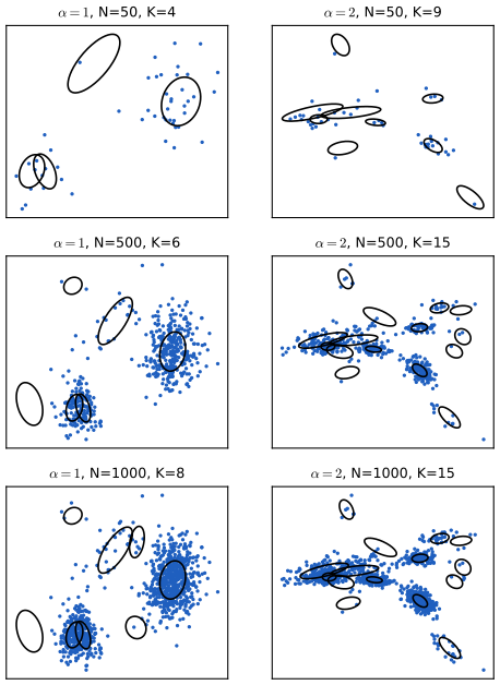
Figure S31.5 of the book (two graphical models for the same DPMM) is a diagram. The DPMM is also the limit of finite mixtures: gap 31.4.
Filling the gap 31.4: the DP mixture is the \(K\to\infty\) limit of finite mixtures with a \(\Dir(\alpha/K)\) prior Supp. p. 274
Proof
Take \(\bm\pi\sim\Dir(\alpha/K,\dots,\alpha/K)\) and \(z_i\sim\Cat(\bm\pi)\). Integrating out \(\bm\pi\) (Dirichlet–multinomial), a labelled assignment with counts \(n_1,\dots,n_K\) has probability \(\frac{\Gamma(\alpha)}{\Gamma(\alpha+N)}\prod_j\frac{\Gamma(\alpha/K+n_j)}{\Gamma(\alpha/K)}\). An unlabelled partition into \(k\) blocks arises from \(K(K-1)\cdots(K-k+1)\) labellings, so
\[ p_K(\text{partition})=\frac{K!}{(K-k)!}\,\frac{\Gamma(\alpha)}{\Gamma(\alpha+N)}\prod_{j=1}^k\frac{\Gamma(\alpha/K+N_j)}{\Gamma(\alpha/K)}. \]As \(K\to\infty\): \(\Gamma(\alpha/K+n)/\Gamma(\alpha/K)=(\alpha/K)(\alpha/K+1)\cdots(\alpha/K+n-1)=(\alpha/K)(n-1)!\,(1+O(1/K))\), and \(K!/(K-k)!=K^k(1+O(1/K))\). The powers of \(K\) cancel and the limit is \(\alpha^k\Gamma(\alpha)/\Gamma(\alpha+N)\prod_j(N_j-1)!\), Ewens's formula. Since the cluster parameters are iid \(H\) in both models, the joint law of the data converges too (Neal 2000; Rasmussen 2000). Numerically, for \(N=7\) and \(\alpha=1.5\) the total-variation-type distance between the laws of the number of used components drops from 0.27 at \(K=10\) to 0.003 at \(K=1000\). ∎
S31.2.2 Fitting using collapsed Gibbs sampling
Supp. pp. 274–276, S(31.20)–S(31.24), Algorithm 31.1 With a conjugate base measure, \(G\) and the cluster parameters can be integrated out and a Gibbs sampler run on the labels alone (Neal 2000, "Algorithm 3"):
\[ p(z_i=k\given\bm z_{-i},\bm x)\propto\begin{cases}N_{k,-i}\;p(x_i\given\bm x_{-i,k}),&k\le K_{-i},\\ \alpha\;p(x_i)=\alpha\int F(x_i\given\theta)H(\d\theta),&k=K_{-i}+1,\end{cases} \tag{S31.20–S31.24} \]where \(\bm x_{-i,k}\) are the other points in cluster \(k\), \(N_{k,-i}\) their number and \(K_{-i}\) the number of clusters once \(i\) is removed (empty clusters deleted). The common factor \(1/(\alpha+N-1)\) cancels.
Algorithm 31.1 (collapsed Gibbs sampler for the DP mixture) Supp. p. 276
Repeat sweeps; in each, visit \(i=1,\dots,N\) in random order: remove \(x_i\)'s sufficient statistics from its cluster (deleting the cluster if it becomes empty); for each existing cluster compute \(N_{k,-i}\,p(x_i\given\bm x_{-i,k})\) and for a new cluster \(\alpha\,p(x_i)\); normalise and draw \(z_i\); add \(x_i\)'s statistics to the chosen cluster. Implemented as dpmm_gibbs with a normal-inverse-Wishart model (Student-\(t\) predictives) and a known-variance Gaussian model.
Filling the gap 31.5: the two factors of the Gibbs conditional Supp. p. 275, S(31.20)–S(31.24)
Derivation
After integrating out \(G\) and the \(\theta\)'s, the joint law of labels and data is \(p(\bm z)\prod_cp(\bm x_c)\), where \(p(\bm z)\) is Ewens's formula and \(p(\bm x_c)=\int\prod_{j:z_j=c}F(x_j\given\theta)H(\d\theta)\) is the marginal likelihood of cluster \(c\) (S31.23); different clusters have independent parameters, so the data factorise across clusters. Hence
\[ p(z_i=k\given\bm z_{-i},\bm x)\propto\frac{p(\bm z_{-i},z_i=k)}{p(\bm z_{-i})}\cdot\frac{\prod_cp(\bm x_c\given z_i=k)}{\prod_cp(\bm x_{-i,c})}. \]Prior factor. By exchangeability the ratio of Ewens probabilities is that of customer \(i\) arriving last: \((N_{k,-i}-1)!\to N_{k,-i}!\) multiplies by \(N_{k,-i}\), a new block multiplies by \(\alpha\) (with \(0!=1\)), and \((\alpha+1)_{N-2}\to(\alpha+1)_{N-1}\) divides by \(\alpha+N-1\): this is (S31.21). Likelihood factor. All clusters except \(k\) cancel, leaving \(p(x_i,\bm x_{-i,k})/p(\bm x_{-i,k})=p(x_i\given\bm x_{-i,k})\) (S31.22), the posterior predictive of cluster \(k\); for a new cluster \(\bm x_{-i,k}\) is empty and the ratio is the prior predictive (S31.24). For the normal-inverse-Wishart base measure the predictive is a multivariate Student \(t\) with \(\nu_n-D+1\) degrees of freedom, location \(\bm m_n\) and scale \(\bm S_n(\kappa_n+1)/(\kappa_n(\nu_n-D+1))\) (gap 3.10).
Validity. Each update draws one coordinate from its exact full conditional, so the posterior over partitions is invariant; the chain is irreducible (any partition can be reached by moving one point at a time) and aperiodic (staying put has positive probability), so it converges (Chapter 12). Numerically, for four 1-d points and a known-variance Gaussian model, the sampler's frequencies over all 15 partitions match the exact posterior computed by enumeration. ∎
S31.2.3 Fitting using variational Bayes
Supp. pp. 277–278, S(31.25)–S(31.34), Algorithm 31.2 Blei and Jordan (2006) work with the stick-breaking representation, latent variables \(\bm w=(\bm\beta,\bm\theta,\bm z)\), and a mean-field family that is truncated at level \(T\) by setting \(q(\beta_T=1)=1\), so \(q\) puts no mass on clusters beyond \(T\) (the model itself is not truncated):
\[ q(\bm\beta,\bm\theta,\bm z)=\prod_{t=1}^{T-1}\Betad(\beta_t\given\gamma_{t,1},\gamma_{t,2})\prod_{t=1}^Tq_{\bm\tau_t}(\theta_t)\prod_{n=1}^N\Cat(z_n\given\bm\phi_n). \tag{S31.31} \]Maximising the ELBO (S31.28) by coordinate ascent, with an exponential-family likelihood \(p(x\given\theta)=h(x)\exp(\theta^{\T}x-a(\theta))\) and its conjugate prior \(p(\theta\given\bm\eta)\propto\exp(\bm\eta_1^{\T}\theta-\eta_2a(\theta))\) (S31.33–S31.34), gives Algorithm 31.2.
Algorithm 31.2 (variational inference for the DP mixture) Supp. p. 278
Initialise \(\bm\phi\). Until the ELBO stops increasing:
\(\gamma_{t,1}=1+\sum_n\phi_{n,t}\), \(\gamma_{t,2}=\alpha+\sum_n\sum_{j=t+1}^T\phi_{n,j}\);
\(\bm\tau_{t,1}=\bm\eta_1+\sum_n\phi_{n,t}x_n\), \(\tau_{t,2}=\eta_2+\sum_n\phi_{n,t}\);
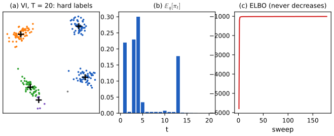
\(\phi_{n,t}\propto\exp(S_{n,t})\) with \(S_{n,t}=\E_q\log\beta_t+\sum_{i\lt t}\E_q\log(1-\beta_i)+\E_q[\theta_t]^{\T}x_n-\E_q[a(\theta_t)]\) (and \(\E_q\log\beta_T=0\)). Implemented as dpmm_vi for Gaussian clusters \(\N(\bm\mu_t,\sigma^2\bm I)\) with \(\bm\mu_t\sim\N(\bm m_0,\rho^2\bm I)\).
Filling the gap 31.6: deriving the three updates, and why the ELBO never decreases Supp. pp. 277–278
Derivation
The CAVI rule (gap 10.11) sets \(\log q(w_j)=\E_{-j}\log p(\bm w,\bm x)+\const\). Write \(\ind(z_n=t)\) and \(\ind(z_n\gt t)\); under the stick-breaking prior, \(\log p(z_n\given\bm\beta)=\sum_t\big[\ind(z_n=t)\log\beta_t+\ind(z_n\gt t)\log(1-\beta_t)\big]\).
Sticks. The terms containing \(\beta_t\) (\(t\lt T\)) are \((\alpha-1)\log(1-\beta_t)\) from the \(\Betad(1,\alpha)\) prior and \(\sum_n[\phi_{n,t}\log\beta_t+\Pr_q(z_n\gt t)\log(1-\beta_t)]\), with \(\Pr_q(z_n\gt t)=\sum_{j\gt t}\phi_{n,j}\). This is the log of a Beta density with \(\gamma_{t,1}=1+\sum_n\phi_{n,t}\) and \(\gamma_{t,2}=\alpha+\sum_n\sum_{j\gt t}\phi_{n,j}\).
Atoms. The terms in \(\theta_t\) are \(\bm\eta_1^{\T}\theta_t-\eta_2a(\theta_t)\) from the prior and \(\sum_n\phi_{n,t}(\theta_t^{\T}x_n-a(\theta_t))\) from the likelihood, so \(q(\theta_t)\) is in the conjugate family with \(\bm\tau_{t,1}=\bm\eta_1+\sum_n\phi_{n,t}x_n\), \(\tau_{t,2}=\eta_2+\sum_n\phi_{n,t}\).
Labels. The terms in \(z_n\) give \(\log q(z_n=t)=\E_q\log\beta_t+\sum_{i\lt t}\E_q\log(1-\beta_i)+\E_q[\theta_t]^{\T}x_n-\E_q a(\theta_t)+\const\), with \(\E_q\log\beta_t=\dg(\gamma_{t,1})-\dg(\gamma_{t,1}+\gamma_{t,2})\) and \(\E_q\log(1-\beta_t)=\dg(\gamma_{t,2})-\dg(\gamma_{t,1}+\gamma_{t,2})\). For the Gaussian model \(\theta=\bm\mu/\sigma^2\), so \(\E[\theta]^{\T}x-\E a(\theta)=-\|x-\bm m_t\|^2/(2\sigma^2)-Ds_t^2/(2\sigma^2)+\const\), where \(q(\bm\mu_t)=\N(\bm m_t,s_t^2\bm I)\) with \(s_t^{-2}=\rho^{-2}+N_t/\sigma^2\) and \(\bm m_t=s_t^2(\bm m_0/\rho^2+\sum_n\phi_{n,t}x_n/\sigma^2)\).
Monotonicity. Each update maximises the ELBO exactly over one block with the others fixed (the ELBO is \(-\Dkl\) between \(q_j\) and the CAVI target, plus a constant), so the ELBO cannot decrease; it is bounded above by \(\log p(\bm x)\), hence it converges. Truncation at \(T\) is part of the variational family, so the ELBO is still a lower bound on the evidence of the untruncated model. In Figure x31.2 the ELBO increases at every sweep and four sticks carry almost all of \(\E_q\bm\pi\). ∎
S31.2.4 Other fitting algorithms
Supp. pp. 278–279 Blocked Gibbs samplers instantiate a truncated \(G\) through its sticks and update all labels in parallel given \(G\) (Ishwaran and James 2001); by gap 31.2 the truncation error is \((\alpha/(1+\alpha))^T\) in mean. Slice samplers remove the truncation by drawing a random level (Kalli, Griffin and Walker 2011). Search (A*, beam search) gives fast approximate MAP clusterings (Daumé 2007), particle filters fit DPMMs online, and several other variational schemes exist. The collapsed sampler of Algorithm 31.1 is the simplest, but it moves one point at a time, which is why the chain in Figure S31.6 is started from many random clusters rather than from one.
S31.2.5 Choosing the hyper-parameters
Supp. p. 279 The concentration has little effect on predictive accuracy but a strong one on the number of clusters (\(\E K_N\approx\alpha\log N\)), so it is usually given a prior. With \(\alpha\sim\Ga(a,b)\) it can be resampled inside the Gibbs sampler, because by Result 31.1 the labels depend on \(\alpha\) only through \(K\): \(p(\alpha\given\bm z)\propto p(\alpha)\,\alpha^K\Gamma(\alpha)/\Gamma(\alpha+N)\) (Escobar and West 1995). Base-measure parameters can be sampled similarly (Rasmussen 2000) or fitted by empirical Bayes (McAuliffe, Blei and Jordan 2006).
Filling the gap 31.7: the Escobar–West auxiliary-variable update for \(\alpha\) Supp. p. 279
Derivation
Use the Beta integral: \(\frac{\Gamma(\alpha)}{\Gamma(\alpha+N)}=\frac{(\alpha+N)}{\alpha\,\Gamma(N)}\int_0^1\eta^{\alpha}(1-\eta)^{N-1}\d\eta\) (since \(B(\alpha+1,N)=\Gamma(\alpha+1)\Gamma(N)/\Gamma(\alpha+N+1)\)). So \(p(\alpha\given K)\) is the marginal of the joint density
\[ p(\alpha,\eta\given K)\propto\Ga(\alpha\given a,b)\,\alpha^{K-1}(\alpha+N)\,\eta^{\alpha}(1-\eta)^{N-1},\qquad0\lt\eta\lt1. \]Its conditionals: \(\eta\given\alpha\sim\Betad(\alpha+1,N)\); and \(p(\alpha\given\eta,K)\propto\alpha^{a+K-2}e^{-\alpha(b-\log\eta)}(\alpha+N)\), which splits the factor \(\alpha+N\) into a two-component mixture
\[ \alpha\given\eta,K\sim w\,\Ga(a+K,\ b-\log\eta)+(1-w)\,\Ga(a+K-1,\ b-\log\eta),\qquad\frac{w}{1-w}=\frac{a+K-1}{N(b-\log\eta)}, \]the odds being the ratio of the two gamma normalisers \(\Gamma(a+K)/(b-\log\eta)^{a+K}\) and \(N\Gamma(a+K-1)/(b-\log\eta)^{a+K-1}\). Alternating the two draws is a Gibbs sampler on \((\alpha,\eta)\) whose \(\alpha\)-marginal is \(p(\alpha\given K)\). Numerically, with \(K=5\), \(N=60\), \(a=2\), \(b=1\), the sampler's mean of \(\alpha\) agrees with the grid posterior mean to two decimals. ∎
S31.3 Generalizations of the Dirichlet process supplement
Supp. p. 279 DP mixtures can be posterior consistent for densities, but as a clustering prior the DP is rigid: one parameter fixes both the number of clusters (\(\approx\alpha\log N\)) and the distribution of their sizes (Result 31.1). Word frequencies, object counts in images and many other quantities follow power laws, which the CRP cannot produce.
S31.3.1 Pitman-Yor process
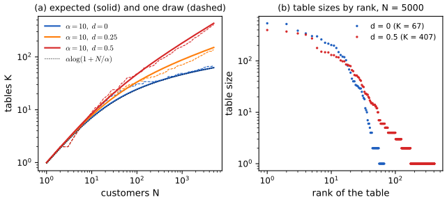
Supp. pp. 279–280, S(31.35)–S(31.38) The Pitman-Yor process \(\PYP(\alpha,d,H)\) (Pitman and Yor 1997) adds a discount \(0\le d\lt1\), with \(\alpha\gt-d\). Its sticks are \(\beta_k\sim\Betad(1-d,\alpha+kd)\) (S31.36); in the restaurant a customer joins table \(k\) with weight \(N_k-d\) and opens a new table with weight \(\alpha+Kd\). Each existing table gives up \(d\) to the new-table option, so the more tables there are, the more likely another one becomes: \(K_N\) grows like \(N^d\) rather than \(\log N\), and the table sizes follow a power law (Figure x31.1). \(d=0\) is the DP.
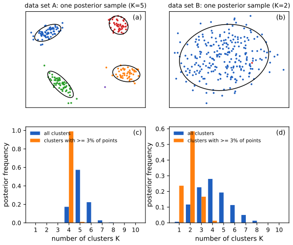
Gibbs-type priors (De Blasi et al. 2013) are exchangeable partition laws of the form \(p(n_1,\dots,n_K)=V_{N,K}\prod_k(1-\sigma)_{n_k-1}\) with \(V_{1,1}=1\) and \(V_{N,K}=(N-\sigma K)V_{N+1,K}+V_{N+1,K+1}\) (S31.38; the supplement prints \((\sigma-1)\), see gap 31.8). They include the DP and PY processes and also priors with an almost surely bounded number of components. That matters because DP and PY mixtures are inconsistent for the number of clusters: if the data come from finitely many clusters, the posterior keeps adding small redundant clusters as \(N\) grows (Miller and Harrison 2014). Figure S31.6 shows the effect at \(N=230\): four large clusters, plus a varying number of tiny ones.
Filling the gap 31.8: the Pitman-Yor partition law, the growth of \(K_N\), coagulation, and Gibbs-type priors Supp. pp. 279–282, S(31.35)–S(31.38), S(31.42)–S(31.44)
Proof
(i) Partition law. As in gap 31.3, multiply the sequential weights. The denominators are again \(\prod_{n=1}^{N-1}(\alpha+n)=(\alpha+1)_{N-1}\) (the weights add to \(\sum_k(N_k-d)+\alpha+Kd=\alpha+n\)). The \(j\)th new table (\(j=2,\dots,K\)) contributes \(\alpha+(j-1)d\), and table \(k\)'s later members contribute \((1-d)(2-d)\cdots(N_k-1-d)=(1-d)_{N_k-1}\). So
\[ p(\text{partition})=\frac{\prod_{i=1}^{K-1}(\alpha+id)}{(\alpha+1)_{N-1}}\prod_{k=1}^K(1-d)_{N_k-1}, \]symmetric in the sizes, hence exchangeable; it sums to one over the 203 partitions of six items (checked numerically).
(ii) Growth. Given the past, the next customer opens a table with probability \((\alpha+dK_n)/(\alpha+n)\), so \(\E K_{n+1}=\E K_n\big(1+\frac{d}{\alpha+n}\big)+\frac{\alpha}{\alpha+n}\), \(\E K_1=1\). For \(d\gt0\) this solves to \(\E K_N=\frac{\alpha}{d}\Big[\frac{(\alpha+d)_N}{(\alpha)_N}-1\Big]=\frac{\alpha}{d}\Big[\frac{\Gamma(\alpha+d+N)\Gamma(\alpha)}{\Gamma(\alpha+d)\Gamma(\alpha+N)}-1\Big]\) (check \(N=1\): \(\frac\alpha d\cdot\frac d\alpha=1\); and that it satisfies the recursion, since \((\alpha+d)_{N+1}/(\alpha)_{N+1}=\frac{(\alpha+d)_N}{(\alpha)_N}\cdot\frac{\alpha+d+N}{\alpha+N}\)). By Stirling, \(\Gamma(x+d)/\Gamma(x)\sim x^d\), so \(\E K_N\sim\frac{\Gamma(\alpha+1)}{d\,\Gamma(\alpha+d)}N^d\): polynomial growth. The recursion, the closed form and simulation agree numerically.
(iii) Stick breaking and ties. Two draws from \(G\) coincide with probability \(\E\sum_k\pi_k^2\). From the restaurant this is the second customer joining the first: \((1-d)/(1+\alpha)\); the stick-breaking simulation with \(\beta_k\sim\Betad(1-d,\alpha+kd)\) gives the same number. (That the PY sticks reproduce the whole PY restaurant is Pitman's theorem; Pitman 2006, Chapter 3.)
(iv) Coagulation, S(31.42)–S(31.44). With \(G_0\sim\PYP(0,d_0,H_0)\) and \(G_1\given G_0\sim\PYP(0,d_1,G_0)\), two draws from \(G_1\) coincide if they sit at the same table of \(G_1\)'s restaurant (probability \(1-d_1\)), or sit at different tables whose dishes, drawn from \(G_0\), coincide (probability \(d_1(1-d_0)\)). Total \(1-d_1+d_1-d_0d_1=1-d_0d_1\), which is the tie probability of \(\PYP(0,d_0d_1,H_0)\) by (iii). This checks the identity on pairs; the full statement is a theorem of Pitman (1999) on coagulation and fragmentation, used by Wood et al. (2009).
(v) Gibbs-type priors. The Pitman-Yor law (i) has the Gibbs form with \(\sigma=d\), weights \((1-\sigma)_{n_k-1}\), and \(V_{N,K}=\prod_{i=1}^{K-1}(\alpha+i\sigma)/(\alpha+1)_{N-1}\). The recursion holds: \((N-\sigma K)V_{N+1,K}+V_{N+1,K+1}=\frac{\prod_{i\lt K}(\alpha+i\sigma)}{(\alpha+1)_N}\big[(N-\sigma K)+(\alpha+K\sigma)\big]=V_{N,K}\), using \((\alpha+1)_N=(\alpha+1)_{N-1}(\alpha+N)\). The recursion is exactly the statement that adding customer \(N+1\) to an existing block of size \(n\) (weight factor \(n-\sigma\), summed to \(N-\sigma K\)) or to a new block gives back the size-\(N\) law, i.e. consistency. The printed factor \((\sigma-1)_{N_k-1}\) cannot be right: for \(\sigma=0\) it is \((-1)(0)(1)\cdots=0\) for every block of size three or more, and with \(\sigma=0.3\), \(\alpha=0.8\) the printed weights summed over the partitions of six items give 0.001 instead of 1. ∎
S31.3.2 Dependent random probability measures
Supp. pp. 280–283, S(31.39)–S(31.49) For grouped data \(\bm X_1,\dots,\bm X_T\), pooling ignores differences and independent DPs ignore shared structure. The hierarchical Dirichlet process (Teh et al. 2006) makes the base measure itself random:
\[ H\sim\DP(\alpha_0,H_0),\qquad G_t\sim\DP(\alpha,H),\qquad\theta^t_i\sim G_t. \tag{S31.39–S31.41} \]Because \(H\) is discrete, every \(G_t\) puts its atoms on the same countable set, so clusters are shared across groups with group-specific weights, and a heavy atom of \(H\) is a priori heavy in every group. Its CRP analogue is the Chinese restaurant franchise (each restaurant's new tables order dishes from a shared upper-level restaurant). Applications include nonparametric topic models (topics are the shared atoms) and the HDP-HMM, where the rows of an infinite transition matrix are tied by an HDP (Fox et al. 2008). Deeper hierarchies (S31.45–S31.48) encode nested group structure, and the PY coagulation property (gap 31.8(iv)) lets the sequence memoizer use infinitely deep hierarchies of which only finitely many levels are instantiated. Covariate-dependent DPs (MacEachern 1999) let the sticks vary smoothly in \(t\), for instance \(\beta^t_k=F^{-1}_{\Betad(1,\alpha)}\big(\Phi(f_k(t))\big)\) with independent unit-variance GPs \(f_k\) (S31.49).
Filling the gap 31.9: the HDP shares atoms, and the GP-transformed sticks have the right marginals Supp. pp. 281–283
Proof
(i) Sharing. Given \(H=\sum_kw_k\delta_{\phi_k}\), the atoms of \(G_t\) are iid draws from \(H\), so they all lie in \(\{\phi_k\}\); hence \(G_t=\sum_k\pi_{tk}\delta_{\phi_k}\) on the common support. The first observations of two different groups coincide exactly when their atoms are the same atom of \(H\): \(\Pr(\theta^1_1=\theta^2_1)=\E\sum_kw_k^2\). For \(\bm w\sim\GEM(\alpha_0)\), \(\E\beta^2=2/((1+\alpha_0)(2+\alpha_0))\) and \(\E(1-\beta)^2=\alpha_0/(\alpha_0+2)\), so \(\E\sum_kw_k^2=\frac{2}{(1+\alpha_0)(2+\alpha_0)}\sum_{k\ge0}\big(\frac{\alpha_0}{\alpha_0+2}\big)^k=\frac{1}{1+\alpha_0}\): the same as the franchise rule "the second table in the upper restaurant joins the first dish". Simulation of the sticks confirms it. Conditionally on \(H\), \(\E[G_t\given H]=H\) and the \(\pi_{tk}\) are positively correlated across groups through \(w_k\).
(ii) Marginals of (S31.49). At a fixed \(t\), \(f_k(t)\sim\N(0,1)\), so \(\Phi(f_k(t))\) is uniform and \(F^{-1}_{\Betad(1,\alpha)}(u)=1-(1-u)^{1/\alpha}\) maps it to a \(\Betad(1,\alpha)\) variable (probability integral transform, gap 2.21); independence over \(k\) is inherited from the GPs. So at each \(t\) the sticks are iid \(\Betad(1,\alpha)\) and \(G_t\sim\DP(\alpha,H)\) marginally, while continuity of the GP paths makes \(G_t\) vary continuously in \(t\). ∎
S31.4 The Indian buffet process and the beta process supplement
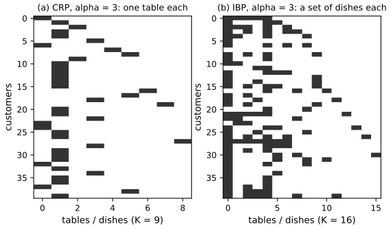
Supp. pp. 283–286, S(31.50)–S(31.52) A clustering is a binary matrix with exactly one 1 per row; a latent feature model lets a row have several 1s (an image contains several objects; a film belongs to several genres). The Indian buffet process (IBP; Griffiths and Ghahramani 2011) is the nonparametric prior on such matrices: customer 1 takes \(\Poi(\alpha)\) dishes; customer \(i\) takes each previously sampled dish \(d\) with probability \(N_d/i\) (\(N_d\) earlier takers) and then \(\Poi(\alpha/i)\) new dishes. Each dish carries a parameter \(\theta_k\sim H\). Rows are exchangeable, so by de Finetti there is a random measure behind them: the beta process \(G=\sum_k\pi_k\delta_{\theta_k}\) with \(\pi_k\in(0,1)\) not summing to one; a row includes feature \(k\) independently with probability \(\pi_k\) (a Bernoulli process). Its stick-breaking form (Teh, Görür and Ghahramani 2007) uses \(\beta_k\sim\Betad(\alpha,1)\) and \(\pi_k=\prod_{l\le k}\beta_l\) (S31.51–S31.52).
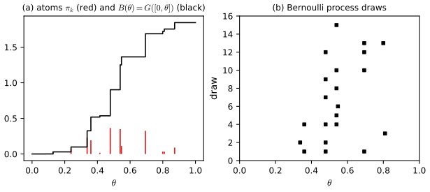
Filling the gap 31.10: each customer takes \(\Poi(\alpha)\) dishes, the buffet has \(\Poi(\alpha H_N)\) dishes, and the sticks have total mass \(\alpha\) Supp. pp. 284–285
Proof
(i) Total dishes. Customer \(i\) adds \(\Poi(\alpha/i)\) new dishes independently of everything else, and a sum of independent Poissons is Poisson, so \(K_N\sim\Poi(\alpha\sum_{i=1}^N1/i)=\Poi(\alpha H_N)\). Since \(H_N\sim\log N\), the number of features grows logarithmically, like the number of CRP tables.
(ii) Dishes per customer. The beta process with mass \(\alpha\) (and concentration 1) is the completely random measure with Lévy intensity \(\alpha w^{-1}\d w\) on \((0,1]\) times \(H\) (S31.6). A row keeps each atom independently with probability \(w\); by the marking theorem the kept atoms form a Poisson process with intensity \(w\cdot\alpha w^{-1}\d w=\alpha\,\d w\) on \((0,1]\), whose total number is \(\Poi(\int_0^1\alpha\,\d w)=\Poi(\alpha)\), finite almost surely. Every row has this law (exchangeability), so the last customer, who takes old dishes with probabilities \(N_d/N\) and \(\Poi(\alpha/N)\) new ones, also takes \(\Poi(\alpha)\) in total. Simulation agrees for \(N=12\) (mean and variance of the last row's count both close to \(\alpha\)).
(iii) Sticks. With \(\beta_l\sim\Betad(\alpha,1)\), \(\E\beta_l=\alpha/(1+\alpha)\), so \(\E\pi_k=(\alpha/(1+\alpha))^k\) and \(\E\sum_k\pi_k=\alpha\): the total mass is finite in mean, hence a.s., and so is the number of features of a row. The weights decrease along the sequence (each is the previous one times a number below one), so the few large atoms are the common features revealed early by the rich-get-richer dynamics. ∎
Three-parameter versions give power laws in the number of features (Teh and Görür 2009); applications include genetics, collaborative filtering and network models, fitted by MCMC, particle filtering or variational methods.
S31.5 Small-variance asymptotics supplement
Supp. pp. 286–289, S(31.53)–S(31.54), Algorithm 31.3 K-means is the \(\sigma^2\to0\) limit of EM for a mixture of Gaussians with shared covariance \(\sigma^2\bm I\) (Volume 1, gap 21.5). Kulis and Jordan (2012) take the same limit of a Gibbs sampler for a DP mixture with cluster means \(\bm\mu\sim\N(\bm 0,\rho^2\bm I)\) and likelihood \(\N(\bm\mu,\sigma^2\bm I)\), with instantiated means. A point joins cluster \(c\) with probability proportional to \(N_{c,-i}\N(\bm x_i\given\bm\mu_c,\sigma^2\bm I)\) and a new cluster with probability proportional to \(\alpha\N(\bm x_i\given\bm 0,(\sigma^2+\rho^2)\bm I)\). Letting \(\sigma^2\to0\) alone would give every point its own cluster; the concentration must vanish too, as
\[ \alpha=\Big(1+\frac{\rho^2}{\sigma^2}\Big)^{D/2}\exp\Big(-\frac{\lambda}{2\sigma^2}\Big). \]The limit is DP-means: assign each point to the nearest centre unless the squared distance exceeds \(\lambda\), in which case it starts a cluster of its own; then recompute the centres as means. It decreases the objective
\[ J(\bm z)=\sum_{k=1}^K\sum_{\bm x\in\mathcal D_k}\|\bm x-\bm\mu_k\|^2+\lambda K,\qquad\bm\mu_k=\frac{1}{|\mathcal D_k|}\sum_{\bm x\in\mathcal D_k}\bm x, \tag{S31.53} \]k-means plus a price \(\lambda\) per cluster, and converges to a local minimum (the supplement says maximum).
Algorithm 31.3 (DP-means) Supp. p. 287
Start with \(K=1\), \(\bm\mu_1=\bar{\bm x}\), all \(z_i=1\). Until no label changes: for \(i=1,\dots,N\), compute \(d_{ik}=\|\bm x_i-\bm\mu_k\|^2\); if \(\min_kd_{ik}\gt\lambda\), set \(K\leftarrow K+1\), \(z_i=K\), \(\bm\mu_K=\bm x_i\); otherwise \(z_i=\argmin_kd_{ik}\). Then set each \(\bm\mu_k\) to the mean of its points (clusters left empty are deleted, which the pseudocode leaves implicit). Implemented as dp_means; try it in the DP-means demonstration.
Filling the gap 31.11: the small-variance limit, and why DP-means decreases (S31.53) Supp. pp. 286–287, "one can show"
Proof
(i) The limit. Substitute the scaling of \(\alpha\) into the new-cluster weight: \(\alpha(2\pi(\sigma^2+\rho^2))^{-D/2}e^{-\|\bm x\|^2/(2(\sigma^2+\rho^2))}=(2\pi\sigma^2)^{-D/2}\exp\big(-\frac{\lambda}{2\sigma^2}-\frac{\|\bm x\|^2}{2(\sigma^2+\rho^2)}\big)\), because \((1+\rho^2/\sigma^2)^{D/2}=((\sigma^2+\rho^2)/\sigma^2)^{D/2}\) cancels the normaliser ratio. An existing cluster has weight \(N_{c,-i}(2\pi\sigma^2)^{-D/2}e^{-\|\bm x-\bm\mu_c\|^2/(2\sigma^2)}\). After removing the common factor \((2\pi\sigma^2)^{-D/2}\), all weights are \(\exp(-(\text{cost})/(2\sigma^2)+O(1))\) with costs \(\|\bm x-\bm\mu_c\|^2\) and \(\lambda\) (the \(\log N_{c,-i}\) and \(\|\bm x\|^2/(2(\sigma^2+\rho^2))\) terms stay bounded). As \(\sigma^2\to0\) the normalised probabilities concentrate on the smallest cost: the nearest centre if its squared distance is below \(\lambda\), a new cluster otherwise. The mean update has posterior \(\N\big(\frac{\sigma^{-2}\sum\bm x}{\rho^{-2}+n\sigma^{-2}},\frac{1}{\rho^{-2}+n\sigma^{-2}}\big)\), which collapses onto the cluster mean. The (supplement's \(1/\sqrt{2\pi\sigma^2}\) is the one-dimensional normaliser; the \(D/2\) power in \(\alpha\) is there to cancel the \(D\)-dimensional one.) A numerical experiment with \(\sigma^2=0.005\): a point at squared distance 1.04 from the nearest centre with \(\lambda=2\) joins it with probability above 0.999; one at squared distance 4.21 opens a new cluster with probability above 0.999.
(ii) Monotonicity. Treat \(J\) as a function of labels and centres, \(J(\bm z,\bm\mu)=\sum_i\|\bm x_i-\bm\mu_{z_i}\|^2+\lambda K\). In the assignment pass, moving \(\bm x_i\) to a nearer existing centre lowers its term; opening a new cluster at \(\bm x_i\) replaces a cost \(\min_kd_{ik}\gt\lambda\) by \(0+\lambda\), also lower; deleting an emptied cluster lowers \(J\) by \(\lambda\). In the update pass, the mean minimises the within-cluster sum of squares (gap 21.4). So \(J\) never increases. There are finitely many partitions, a partition can only recur with the same \(J\), and the loop stops when labels repeat, so the algorithm terminates at a point where no single reassignment and no mean update helps: a local minimum, typically not the global one (Figure x31.3(a) splits two true clusters). At convergence every point is within squared distance \(\lambda\) of its centre. ∎
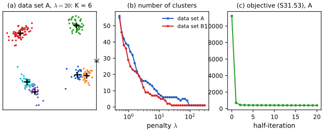
The same limit of an HDP sampler gives a hard clustering of several data sets with a local penalty \(\lambda_l\) (a cluster new to a data set) and a global one \(\lambda_g\) (a new cluster overall). For exponential-family mixtures the squared distance becomes the Bregman divergence of the family (Jiang, Kulis and Jordan 2012). MAD-Bayes (Broderick, Kulis and Jordan 2013) takes the limit of the MAP objective directly; for the IBP it gives BP-means, \(\min_{K,\bm Z,\bm A}\Tr[(\bm X-\bm Z\bm A)^{\T}(\bm X-\bm Z\bm A)]+\lambda K\) (S31.54): reconstruction error plus a price per feature, decreased by alternating row-wise updates of \(\bm Z\), proposing a new feature equal to a row's residual, and a least-squares update of \(\bm A\). (The price \(\lambda K\) resembles the AIC or BIC penalty in form, a constant per component, but \(\lambda\) is a tuning parameter, not twice the parameter count.)
See also. Volume 1, Section 21.3 (k-means and choosing \(K\)).
S31.6 Completely random measures supplement
Supp. pp. 289–290, S(31.55) A random measure \(G\) is completely random (a CRM; Kingman 1967) if its masses on disjoint sets are independent (S31.55). The DP is not: \(G(T)=1-G(T^c)\), and in general \(\cov(G(T_1),G(T_2))=-H(T_1)H(T_2)/(1+\alpha)\) for disjoint sets (a Dirichlet covariance). The simplest CRM is the Poisson process viewed as a counting measure. Every CRM without fixed atoms is built from a Poisson process: take a Poisson process \(\{(\theta_i,w_i)\}\) on \(\Theta\times(0,\infty)\) with intensity \(\lambda(\theta,w)=H(\theta)\gamma(w)\) and set \(G=\sum_iw_i\delta_{\theta_i}\) (Figure S31.9). Choices of the Lévy density \(\gamma\) give the gamma process (\(\alpha w^{-1}e^{-w}\)), the beta process (\(\alpha w^{-1}\) on \((0,1]\) for the IBP of S31.4; more generally \(c\,\alpha w^{-1}(1-w)^{c-1}\)), the stable process (\(\propto w^{-1-\sigma}\)) and the generalised gamma process (\(\propto w^{-1-\sigma}e^{-\zeta w}\)). When \(\int\gamma=\infty\) there are infinitely many atoms, and when \(0\lt G(\Theta)\lt\infty\) the normalised measure \(G/G(\Theta)\) is a random probability measure, a normalised random measure. The DP is the normalised gamma process; the normalised stable process is \(\PYP(0,\sigma)\), and PY is not an NRM otherwise.
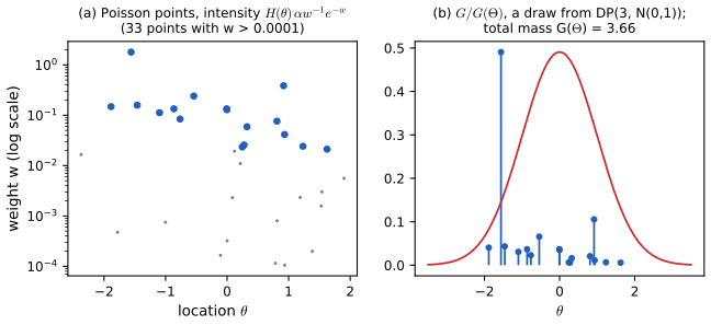
Filling the gap 31.12: the Laplace functional of a CRM, when the total mass is finite, and why the normalised gamma process is a DP Supp. p. 290, "it is easy to show"
Proof
(i) Laplace functional. For a Poisson process with intensity \(\lambda\) and \(f\ge0\), Campbell's theorem gives \(\E e^{-\sum_if(\theta_i,w_i)}=\exp\{-\int(1-e^{-f})\,\d\lambda\}\). With \(f=tw\ind(\theta\in T)\), \(\E e^{-tG(T)}=\exp\{-H(T)\int_0^\infty(1-e^{-tw})\gamma(w)\,\d w\}\). Disjoint sets use disjoint parts of the Poisson process, which are independent, so \(G\) is completely random.
(ii) Finite and positive mass. \(G(\Theta)\lt\infty\) a.s. iff \(\int_0^\infty\min(1,w)\gamma(w)\,\d w\lt\infty\): the atoms with \(w\gt1\) are finitely many iff \(\int_1^\infty\gamma\lt\infty\), and the small atoms have finite total mean \(\int_0^1w\gamma(w)\d w\) (and conversely, if that integral is infinite, the exponent in (i) is infinite for every \(t\gt0\), so \(G(\Theta)=\infty\) a.s.). The supplement's condition "\(\int_\epsilon^\infty\gamma\lt\infty\) for every \(\epsilon\)" only controls the number of large atoms and is not enough on its own: \(\gamma(w)=w^{-2}\) on \((0,1)\) satisfies it but gives infinite mass. \(G(\Theta)\gt0\) a.s. iff \(\int\gamma=\infty\) (otherwise there are no atoms at all with probability \(e^{-\int\gamma}\gt0\)). All four examples satisfy both conditions (for the stable one, \(0\lt\sigma\lt1\)).
(iii) Gamma process. With \(\gamma(w)=\alpha w^{-1}e^{-w}\), Frullani's integral gives \(\int_0^\infty(1-e^{-tw})w^{-1}e^{-w}\d w=\log(1+t)\), so \(\E e^{-tG(T)}=(1+t)^{-\alpha H(T)}\): \(G(T)\sim\Ga(\alpha H(T),1)\), independent over disjoint sets. For a partition, \((G(T_j)/G(\Theta))_j\) is a vector of independent gammas divided by their sum, which is \(\Dir(\alpha H(T_1),\dots,\alpha H(T_K))\) and independent of the sum (gap 2.6). That is definition (S31.1): \(G/G(\Theta)\sim\DP(\alpha,H)\), independently of the total mass \(G(\Theta)\sim\Ga(\alpha,1)\). Simulated gamma-process masses have mean and variance close to \(\alpha\). ∎
S31.7 Lévy processes supplement
Supp. pp. 290–291 A Lévy process \((L_t)_{t\ge0}\) has stationary and independent increments (and is continuous in probability). A non-decreasing one is a subordinator; its jumps are the atoms of a CRM on \([0,\infty)\) with Lebesgue base measure (the black staircase of Figure S31.8 is a beta subordinator). Increments of a general Lévy process are infinitely divisible; conversely every infinitely divisible law is the law of \(L_1\) for some Lévy process (Lévy–Khintchine), and every Lévy process is a drift plus a Brownian part plus a Poisson jump part (Lévy–Itô). Brownian motion has increments \(L_{t+\Delta}-L_t\sim\N(\mu\Delta,\sigma^2\Delta)\) and continuous paths; all other Lévy processes jump.
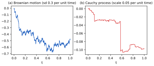
Filling the gap 31.13: increments are infinitely divisible, and the Gaussian, Poisson, gamma and Cauchy examples Supp. p. 291
Proof
Split \([t,t+\Delta]\) into \(n\) equal pieces: \(L_{t+\Delta}-L_t\) is the sum of \(n\) increments that are independent (independent increments) and identically distributed (stationarity), so its law is an \(n\)-fold convolution power for every \(n\). In terms of characteristic functions, \(\varphi_\Delta(s)=\varphi_{\Delta/n}(s)^n\), so \(\varphi_\Delta=\varphi_1^\Delta\) (for rational, then by continuity all \(\Delta\)). Examples: \(\N(\mu,\sigma^2)\) has \(\varphi_1^{1/n}\) equal to the characteristic function of \(\N(\mu/n,\sigma^2/n)\); \(\Poi(\lambda)\) of \(\Poi(\lambda/n)\); \(\Ga(a,b)\) of \(\Ga(a/n,b)\); the Cauchy law with scale \(c\), \(\varphi(s)=e^{-c|s|}\), of the Cauchy with scale \(c/n\). So Cauchy increments over \(\Delta\) have scale \(c\Delta\), which is how Figure S31.10(b) is simulated, and a sum of eight Cauchy(1/8) variables passes a Kolmogorov–Smirnov test against Cauchy(1). Note that for Brownian motion the variance grows like \(\Delta\) (the supplement writes \(\N(\mu\Delta,\sigma\Delta)\)). ∎
S31.8 Point processes with repulsion and reinforcement supplement
S31.8.1 Poisson process
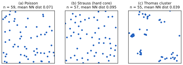
Supp. pp. 292–293 A Poisson process with intensity \(\lambda(\theta)\ge0\) puts a \(\Poi(\int_T\lambda)\) number of points in each set \(T\), independently over disjoint sets (homogeneous if \(\lambda\) is constant). When \(\Lambda=\int_\Theta\lambda\lt\infty\) it can be simulated by drawing \(N\sim\Poi(\Lambda)\) and then \(N\) iid locations from \(\lambda/\Lambda\); on the line, a homogeneous process has iid \(\mathrm{Exp}(\lambda)\) gaps. If \(\Lambda\) is hard to compute, thinning (Lewis and Shedler 1979) simulates a process with a dominating intensity \(\gamma\ge\lambda\) and keeps each point \(\psi\) with probability \(\lambda(\psi)/\gamma(\psi)\). Real patterns are often underdispersed (regular: trees competing for light) or overdispersed (clustered: aftershocks). Cox processes, \(\lambda(\theta)=g(\ell(\theta))\) with \(\ell\) a GP (S31.56), model overdispersion through a random intensity, but not direct interaction between points.
Filling the gap 31.14: why the two-step simulation and thinning give Poisson processes Supp. p. 292, "one can show"
Proof
(i) Two-step simulation. Let \(N\sim\Poi(\Lambda)\) and, given \(N\), let the points be iid with density \(\lambda/\Lambda\). For disjoint \(T_1,\dots,T_m\) covering \(\Theta\), the counts given \(N\) are multinomial with probabilities \(p_j=\Lambda_j/\Lambda\), \(\Lambda_j=\int_{T_j}\lambda\). Then \(\Pr(n_1,\dots,n_m)=e^{-\Lambda}\frac{\Lambda^N}{N!}\cdot\frac{N!}{\prod n_j!}\prod p_j^{n_j}=\prod_je^{-\Lambda_j}\frac{\Lambda_j^{n_j}}{n_j!}\): independent \(\Poi(\Lambda_j)\) counts, which is the definition.
(ii) Exponential gaps. On the line with constant rate, \(\Pr(\text{first point after }t)=\Pr(N(0,t]=0)=e^{-\lambda t}\), and by independence of increments the same holds after every point, so the gaps are iid exponential; memorylessness \(\Pr(\tau\gt\Delta+\delta\given\tau\gt\delta)=e^{-\lambda\Delta}\) is the same fact.
(iii) Thinning. Keeping each point of a rate-\(\gamma\) process independently with probability \(p(\psi)=\lambda(\psi)/\gamma(\psi)\) gives, conditionally on the \(N\) proposed points, kept points that are iid with density proportional to \(\gamma p=\lambda\), each kept with probability \(\int\lambda/\int\gamma\). So the number kept is a \(\Poi(\int\gamma)\) count thinned binomially, which is \(\Poi(\int\lambda)\), and the kept locations are iid \(\lambda/\int\lambda\): by (i), a Poisson process with intensity \(\lambda\). Simulated counts on \([0,10]\) with \(\lambda(t)=2+1.5\sin t\) have mean and variance equal to \(\int_0^{10}\lambda\). ∎
S31.8.2 Renewal process
Supp. p. 293 A renewal process on the line has iid gaps from a general distribution on \((0,\infty)\), so the time since the last event matters. Gamma and Weibull renewal processes contain the Poisson process (shape 1) and allow burstiness (events cluster: shape below 1, decreasing hazard) or refractoriness (events avoid each other: shape above 1, increasing hazard), as for email traffic and neural spikes respectively.
Filling the gap 31.15: the hazard decides burstiness or refractoriness Supp. p. 293
Derivation
The intensity of a renewal process at time \(t\) is the hazard of the gap distribution evaluated at the time since the last event, \(h(u)=f(u)/(1-F(u))\). For the Weibull law with shape \(k\) and scale \(s\), \(h(u)=(k/s)(u/s)^{k-1}\): decreasing for \(k\lt1\) (an event makes another one more likely soon after: bursty), constant for \(k=1\) (Poisson), increasing for \(k\gt1\) (a recovery period: refractory). For the gamma law with shape \(a\) the hazard is decreasing for \(a\lt1\) and increasing for \(a\gt1\), tending to the rate in both cases (a standard consequence of log-convexity or log-concavity of the density). The coefficient of variation of the gaps, \(1/\sqrt a\) for the gamma, is above 1 for bursty and below 1 for regular trains. ∎
S31.8.3 Hawkes process
Supp. pp. 294–296, S(31.57)–S(31.59) A Hawkes process (Hawkes 1971) is self-exciting: its conditional intensity given the history \(\Hc(t)=\{t_k\le t\}\) is
\[ \lambda(t\given\Hc(t))=\gamma+\sum_{t_k\in\Hc(t)}\phi(t-t_k), \tag{S31.57} \]with base rate \(\gamma\) and triggering kernel \(\phi\), typically \(\phi(\Delta)=\beta e^{-\Delta/\tau}\): each event raises the intensity by \(\beta\), and the excess decays back to \(\gamma\) on the time scale \(\tau\). A multivariate version has \(\lambda_i=\gamma_i+\sum_j\sum_{t_k\in\Hc_j}\phi_{ij}(t-t_k)\) (S31.58), with \(\phi_{ij}=0\) when \(j\) cannot influence \(i\). Simulation follows the intensity forward in time (Ogata's thinning: between events the exponential-kernel intensity only decreases, so its current value bounds it until the next event), and the log-likelihood of events \(\Psi\) on \([0,T]\) is
\[ \ell(\Psi)=\sum_{t^*\in\Psi}\log\lambda(t^*\given\Hc(t^*))-\int_0^T\lambda(t\given\Hc(t))\,\d t. \tag{S31.59} \]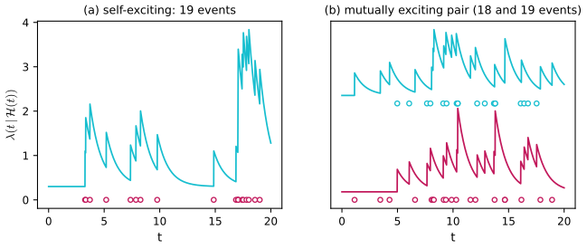
Filling the gap 31.16: the likelihood (S31.59), its \(O(N)\) recursion, stationarity, and the mean number of events Supp. pp. 294–295
Derivation
(i) Likelihood. Given the history up to the \(i\)th event, the next event time has hazard \(\lambda(t\given\Hc(t_i))\) on \((t_i,\infty)\), so its density is \(\lambda(t_{i+1}\given\Hc)\exp\{-\int_{t_i}^{t_{i+1}}\lambda\}\), and the probability of no event in \((t_N,T]\) is \(\exp\{-\int_{t_N}^T\lambda\}\). Multiplying the conditional densities (chain rule) and taking logs gives (S31.59).
(ii) Exponential kernel. With \(A_i=\sum_{k\lt i}e^{-(t_i-t_k)/\tau}\) we have \(A_1=0\) and \(A_i=e^{-(t_i-t_{i-1})/\tau}(1+A_{i-1})\), so \(\sum_i\log(\gamma+\beta A_i)\) costs \(O(N)\); the compensator is \(\int_0^T\lambda=\gamma T+\beta\tau\sum_i(1-e^{-(T-t_i)/\tau})\). Both agree with a direct double sum and numerical quadrature, and maximising \(\ell\) on a long simulated record recovers \((\gamma,\beta,\tau)\).
(iii) Branching structure and stationarity. Each event triggers offspring events forming a Poisson process with intensity \(\phi\), so it has on average \(n=\int_0^\infty\phi=\beta\tau\) direct offspring (the branching ratio). If \(n\lt1\) the clusters are finite and the process can be stationary, with mean rate \(m_\infty\) solving \(m_\infty=\gamma+n\,m_\infty\), i.e. \(m_\infty=\gamma/(1-\beta\tau)\); if \(n\ge1\) it explodes.
(iv) Mean count from an empty history. The mean intensity \(m(t)=\E\lambda(t)\) satisfies \(m(t)=\gamma+\int_0^t\beta e^{-(t-s)/\tau}m(s)\,\d s\). Differentiating, \(m'=\beta m-(m-\gamma)/\tau\), a linear ODE with \(m(0)=\gamma\), whose solution is \(m(t)=m_\infty+(\gamma-m_\infty)e^{-(1-n)t/\tau}\). Integrating,
\[ \E N(T)=m_\infty T+(\gamma-m_\infty)\frac{\tau}{1-n}\big(1-e^{-(1-n)T/\tau}\big),\qquad n=\beta\tau. \]For \(\gamma=0.5\), \(\beta=0.6\), \(\tau=1\), \(T=50\): \(m_\infty=1.25\) and \(\E N(50)=62.5-1.875(1-e^{-20})=60.625\), matching the average of 4000 simulated records. ∎
The Hawkes demonstration simulates the process with adjustable \(\gamma,\beta,\tau\), draws the intensity and reports the log-likelihood and the expected count; preset 4 shows an explosive process with \(\beta\tau\gt1\). Extensions cluster the nodes of a network with a DP (Blundell, Beck and Heller 2012), let the jump depend on a mark through a GP (Tan et al. 2016), or drive the intensity with a continuous-time LSTM (the neural Hawkes process, Mei and Eisner 2017).
S31.8.4 Gibbs point process
Supp. pp. 296–297, S(31.60)–S(31.63) In higher dimensions there is no "history", so Gibbs point processes specify a density with respect to a unit-rate Poisson process, \(P_\beta(\Psi)=Z_\beta^{-1}\exp(-\beta E(\Psi))\) (S31.60), typically with pairwise energies \(E(\Psi)=\sum_{\{s,s'\}}\phi(\|s-s'\|)\) (S31.61). The Strauss process uses \(\phi=a\,\ind(\|s-s'\|\le R)\) (S31.62), penalising close pairs; \(a\to\infty\) gives a hard core. Piecewise-constant, smooth and higher-order (triplet, area-interaction) energies are also used. The normaliser \(Z_\beta\) is an infinite-dimensional integral, so fitting uses pseudo-likelihood.
Filling the gap 31.17: the Papangelou intensity, the birth-death sampler, and the pseudo-likelihood Supp. pp. 296–297
Derivation
Add an activity \(\kappa\) for the number of points (otherwise the Strauss density cannot set the mean count): \(f(\Psi)\propto\kappa^{|\Psi|}\gamma_s^{s(\Psi)}\) with \(\gamma_s=e^{-\beta a}\in[0,1]\) and \(s(\Psi)\) the number of \(R\)-close pairs. The Papangelou conditional intensity \(\lambda^*(u;\Psi)=f(\Psi\cup\{u\})/f(\Psi)=\kappa\gamma_s^{t(u,\Psi)}\), with \(t(u,\Psi)\) the number of points of \(\Psi\) within \(R\) of \(u\), does not involve \(Z\). Birth-death MH (Geyer and Møller 1994) on the unit square proposes, with probability \(\frac12\) each, a birth at a uniform \(u\) or the death of a uniformly chosen point; detailed balance with respect to \(f\) (density relative to a unit-rate Poisson process on a set of area 1) gives acceptance probabilities \(\min\{1,\lambda^*(u;\Psi)/(|\Psi|+1)\}\) for a birth and \(\min\{1,|\Psi|/\lambda^*(u;\Psi\setminus u)\}\) for the death of \(u\). With \(\gamma_s=0\) a birth inside the hard core is always rejected, so no two points are ever closer than \(R\) (checked on the simulated pattern of Figure S31.11(b)). The pseudo-likelihood \(\prod_{s\in\Psi}\lambda^*(s;\Psi\setminus s)\exp\{-\int\lambda^*(u;\Psi)\d u\}\) replaces \(f\) by a product of conditionals (Besag's idea), which avoids \(Z\) and gives consistent estimates under mixing conditions. ∎
S31.8.5 Determinantal point process
Supp. pp. 297–299, S(31.64)–S(31.68) A determinantal point process (DPP) on a ground set \(S\) (here finite, \(|S|=M\)) is a random subset \(Y\) with
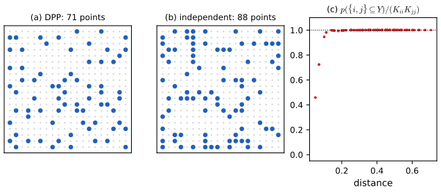
\[ \Pr(A\subseteq Y)=\det(\bm K_A)\quad\text{for all }A\subseteq S, \tag{S31.64} \]for a marginal kernel \(\bm K\) with \(\bm 0\preceq\bm K\preceq\bm I\) (positive semidefinite, eigenvalues in \([0,1]\)). So \(\Pr(i\in Y)=K_{ii}\) (S31.65) and \(\Pr(\{i,j\}\subseteq Y)=K_{ii}K_{jj}-K_{ij}^2\) (S31.66): similar items repel. An L-ensemble specifies the probabilities of exact configurations, \(\Pr(Y=A)\propto\det(\bm L_A)\) with \(\bm L\succeq\bm 0\) (S31.67), and
\[ \Pr(Y=A)=\frac{\det(\bm L_A)}{\det(\bm L+\bm I)},\qquad \bm K=\bm L(\bm L+\bm I)^{-1}=\bm I-(\bm L+\bm I)^{-1}. \tag{S31.68} \](The supplement prints the normaliser as \(\bm I+\det(\bm L)\) and \(\det(\bm K)\) for \(\det(\bm K_A)\).) For a Gram matrix \(\bm L=\bm B^{\T}\bm B\), \(\det(\bm L_A)\) is the squared volume of the parallelotope spanned by the columns of \(\bm B\) indexed by \(A\) (Figure S31.13 of the book is a diagram of this), so diverse sets are favoured.
Filling the gap 31.18: the L-ensemble normaliser and marginal kernel, and the spectral sampler Supp. pp. 297–299, "it is not hard to show", "one can show"
Proof
(i) A determinant expansion. For a diagonal \(\bm D=\diag(d_1,\dots,d_M)\), multilinearity of the determinant in the columns gives \(\det(\bm L+\bm D)=\sum_{A\subseteq S}\det(\bm L_A)\prod_{i\notin A}d_i\) (expand each column \(\bm l_i+d_i\bm e_i\); choosing \(\bm e_i\) for \(i\notin A\) leaves the principal minor on \(A\)). With \(\bm D=\bm I\): \(\sum_A\det(\bm L_A)=\det(\bm L+\bm I)\), the normaliser.
(ii) Marginals. With \(\bm I_{\bar A}\) the diagonal indicator of \(S\setminus A\), the same expansion gives \(\sum_{B\supseteq A}\det(\bm L_B)=\det(\bm L+\bm I_{\bar A})\). Hence \(\Pr(A\subseteq Y)=\det\big((\bm L+\bm I-\bm I_A)(\bm L+\bm I)^{-1}\big)=\det\big(\bm I-\bm I_A(\bm L+\bm I)^{-1}\big)\). The rows of this matrix outside \(A\) are rows of the identity, so its determinant equals that of its \(A\times A\) block, which is \([\bm I-(\bm L+\bm I)^{-1}]_A=\bm K_A\). So L-ensembles are DPPs with \(\bm K=\bm I-(\bm L+\bm I)^{-1}=\bm L(\bm L+\bm I)^{-1}\), whose eigenvalues \(\lambda/(1+\lambda)\) lie in \([0,1)\). (Not every DPP is an L-ensemble: \(\bm K\) with an eigenvalue 1 has no \(\bm L\).) Repulsion: \(\Pr(\{i,j\}\subseteq Y)-K_{ii}K_{jj}=-K_{ij}^2\le0\).
(iii) Mixture of projection DPPs. Let \(\bm L=\sum_j\lambda_j\bm v_j\bm v_j^{\T}\). By Cauchy–Binet, \(\det(\bm L_A)=\sum_{|J|=|A|}\prod_{j\in J}\lambda_j\det(\bm V_{A,J})^2\), and for a set \(J\) of orthonormal eigenvectors, \(\det(\bm V_{A,J})^2\) (with \(|A|=|J|\)) is the probability law of the projection DPP with kernel \(\bm V_J\bm V_J^{\T}\), which always has exactly \(|J|\) points. Dividing by \(\det(\bm L+\bm I)=\prod_j(1+\lambda_j)\),
\[ \Pr(Y=A)=\sum_J\Big[\prod_{j\in J}\frac{\lambda_j}{1+\lambda_j}\prod_{j\notin J}\frac{1}{1+\lambda_j}\Big]\det(\bm V_{A,J})^2: \]first keep each eigenvector independently with probability \(\lambda_j/(1+\lambda_j)\) (the eigenvalue of \(\bm K\), as in the supplement's Bernoulli description), then sample the projection DPP: pick item \(i\) with probability \(\frac1{|J|}\sum_{\bm v\in J}v_i^2\), restrict the span to vectors vanishing at \(i\), and repeat (Hough et al. 2006; Kulesza and Taskar 2012). In particular \(\E|Y|=\sum_j\lambda_j/(1+\lambda_j)=\Tr\bm K\). My implementation reproduces the exact law of all 64 subsets of a six-item ground set (total-variation distance 0.017 with 40,000 draws, the size expected from sampling noise). ∎
Practice problems
The chapter has no exercises, so here are three short problems of my own, with complete solutions (hidden).
Practice problem 31.1 (a partition probability). Under a CRP with \(\alpha=1\), find the probability that four customers end up in the partition \(\{\{1,2\},\{3\},\{4\}\}\), compare with what the printed S(31.15) gives, and find \(\E K_4\).
Solution
Sequentially: customer 1 opens a table (1); customer 2 joins it (\(1/(1+1)=1/2\)); customer 3 opens a table (\(\alpha/(\alpha+2)=1/3\)); customer 4 opens a table (\(1/4\)). Product \(1/24\). Ewens's formula (Result 31.1): \(\alpha^{K-1}\prod(N_k-1)!/(\alpha+1)_{3}=1\cdot1/(2\cdot3\cdot4)=1/24\). The printed formula gives \(\alpha^{2}\prod N_k!/[(2)(3)(4)(5)]=2/120=1/60\). \(\E K_4=1+\frac12+\frac13+\frac14=\frac{25}{12}\approx2.083\).
Practice problem 31.2 (a stationary Hawkes process). A Hawkes process has \(\gamma=0.5\), \(\phi(\Delta)=0.6e^{-\Delta}\). (a) Is it stationary, and what is its long-run rate? (b) What fraction of events are "immigrants" (triggered by the base rate)? (c) Starting from an empty history, what is \(\E N(100)\)?
Solution
(a) The branching ratio is \(n=\beta\tau=0.6\lt1\), so yes; the rate is \(\gamma/(1-n)=1.25\) events per unit time. (b) Immigrants arrive at rate \(\gamma=0.5\), so the fraction is \(0.5/1.25=1-n=0.4\); each immigrant heads a cluster of mean size \(1/(1-n)=2.5\). (c) By gap 31.16(iv), \(\E N(100)=1.25\cdot100+(0.5-1.25)\cdot\frac{1}{0.4}(1-e^{-40})=125-1.875=123.125\). This is the "expected count" shown by preset 1 of the demonstration.
Practice problem 31.3 (a two-item DPP). Let \(\bm L=\begin{pmatrix}1&0.5\\0.5&1\end{pmatrix}\). Find the four probabilities \(\Pr(Y=A)\), the marginal kernel \(\bm K\), and check that the two items are negatively correlated.
Solution
\(\det(\bm L+\bm I)=2\cdot2-0.25=3.75\). \(\Pr(\emptyset)=1/3.75=0.267\), \(\Pr(\{1\})=\Pr(\{2\})=1/3.75=0.267\), \(\Pr(\{1,2\})=(1-0.25)/3.75=0.2\); they sum to one. \((\bm L+\bm I)^{-1}=\frac{1}{3.75}\begin{pmatrix}2&-0.5\\-0.5&2\end{pmatrix}\), so \(\bm K=\bm I-(\bm L+\bm I)^{-1}\) has \(K_{11}=K_{22}=1-2/3.75=0.467\) (indeed \(0.267+0.2\)) and \(K_{12}=0.5/3.75=0.133\). Then \(\det\bm K=0.2178-0.0178=0.2=\Pr(\{1,2\}\subseteq Y)\), below \(K_{11}K_{22}=0.218\): including one item makes the other less likely.
Demonstrations
- The Chinese restaurant and Pitman-Yor processes (Sections S31.1.3 and S31.3.1): seat \(N\) customers with concentration \(\alpha\) and discount \(d\); the tables, their sizes by rank, and the number of tables against its exact expectation.
- DP-means clustering (Section S31.5): Algorithm 31.3 on the two data sets of Figure S31.6, step by step, with the penalty \(\lambda\), the clusters, and the objective (S31.53).
- Hawkes processes (Section S31.8.3): simulate a self-exciting process by thinning, watch the intensity, and compare the count and the log-likelihood with the formulas of gap 31.16.
Python code for every figure: code index. Data used by the demos: data/ch31-dpmeans.json.
Notes on the book
Points where the book or its supplement is imprecise or wrong
- Section 31.1 (book). The Gram matrix is written \([K(x_i),K(x_j)]\); it is \([K(x_i,x_j)]_{ij}\).
- S(31.6). The posterior Dirichlet parameters are \(\alpha H(T_k)+\sum_i\ind(\theta_i\in T_k)\), not \(G(T_k)+\dots\) (the random quantity \(G(T_k)\) cannot be a parameter of its own posterior). The conclusion (S31.7) is right.
- S(31.15). Ewens's formula should read \(\alpha^{K-1}\prod_k(N_k-1)!/(\alpha+1)_{N-1}\); the printed \(\alpha^{K-1}\prod_kN_k!/[\alpha+1]^N\) gives \(1/(1+\alpha)\) for \(N=1\) and does not sum to one over partitions (gap 31.3, problem 31.1). It is also the probability of one particular partition, not of the size vector \((N_1,\dots,N_K)\) as the notation \(p(N_1,\dots,N_k)\) suggests.
- Section S31.1.3. "\(K\) approaches \(\alpha\log N\) almost surely": it is the ratio \(K_N/\log N\) that converges to \(\alpha\); the difference \(K_N-\alpha\log N\) has variance growing like \(\alpha\log N\) (gap 31.3).
- Section S31.3.1. The discount must satisfy \(0\le d\lt1\) (not "greater than 0": \(d=0\) is the DP, which the text then uses; and \(\Betad(1-d,\cdot)\) needs \(d\lt1\)); "observations \(\theta_1,\dots,\theta_d\)" should be \(\theta_1,\dots,\theta_N\).
- S(31.38). The Gibbs-type weights are \((1-\sigma)_{N_k-1}\), not \((\sigma-1)_{N_k-1}\), which vanishes for \(\sigma=0\) and blocks of size 3 or more (gap 31.8).
- S(31.52). "\(\pi_k=\beta_k\pi_{k1}\)" is \(\beta_k\pi_{k-1}\).
- Section S31.5. DP-means converges to a local minimum of (S31.53), not a maximum. The Gaussian normaliser written \(1/\sqrt{2\pi\sigma^2}\) is the one-dimensional one; in \(D\) dimensions it is \((2\pi\sigma^2)^{-D/2}\), which is what the \(D/2\) power in the scaling of \(\alpha\) cancels (gap 31.11).
- Section S31.6. The beta process density \(w^{-1}(1-w)^{\alpha-1}\) uses \(\alpha\) as a concentration with mass 1, while S(31.51) and the IBP use \(\alpha\) as the mass with concentration 1 (Lévy density \(\alpha w^{-1}\) on \((0,1]\)); with the printed density a row would have \(1/\alpha\) features on average, not \(\alpha\) (gap 31.10). Also, finiteness of the total mass needs \(\int_0^1w\gamma(w)\,\d w\lt\infty\) in addition to \(\int_\epsilon^\infty\gamma\lt\infty\) (gap 31.12).
- Section S31.7. Brownian increments are \(\N(\mu\Delta,\sigma^2\Delta)\); the printed \(\N(\mu\Delta,\sigma\Delta)\) has the variance wrong unless \(\sigma\) denotes a variance.
- Section S31.8.5. \(\bm K\) need only be positive semidefinite (\(\bm 0\preceq\bm K\)), not positive definite; the L-ensemble normaliser is \(\det(\bm L+\bm I)\), not "\(\bm I+\det(\bm L)\)"; the marginal statement is \(\Pr(A\subseteq Y)=\det(\bm K_A)\), not \(\det(\bm K)\); and \(\det(\bm L_A)\) is a squared volume (gap 31.18).
References
- Murphy, K. P. (2023). Probabilistic Machine Learning: Advanced Topics. MIT Press, Cambridge, MA. Chapter 31, pp. 1081–1082, and supplementary material, Chapter 31, pp. 267–300. probml.github.io/pml-book/book2.html.
- Antoniak, C. E. (1974). Mixtures of Dirichlet processes with applications to Bayesian nonparametric problems. Annals of Statistics, 2(6), 1152–1174.
- Blackwell, D. and MacQueen, J. B. (1973). Ferguson distributions via Pólya urn schemes. Annals of Statistics, 1(2), 353–355.
- Blei, D. M. and Jordan, M. I. (2006). Variational inference for Dirichlet process mixtures. Bayesian Analysis, 1(1), 121–143.
- Blundell, C., Beck, J. and Heller, K. A. (2012). Modelling reciprocating relationships with Hawkes processes. Advances in Neural Information Processing Systems, 25.
- Broderick, T., Kulis, B. and Jordan, M. I. (2013). MAD-Bayes: MAP-based asymptotic derivations from Bayes. International Conference on Machine Learning.
- De Blasi, P., Favaro, S., Lijoi, A., Mena, R. H., Prünster, I. and Ruggiero, M. (2013). Are Gibbs-type priors the most natural generalization of the Dirichlet process? IEEE Transactions on Pattern Analysis and Machine Intelligence, 37(2), 212–229.
- Escobar, M. D. and West, M. (1995). Bayesian density estimation and inference using mixtures. Journal of the American Statistical Association, 90(430), 577–588.
- Ewens, W. J. (1972). The sampling theory of selectively neutral alleles. Theoretical Population Biology, 3(1), 87–112.
- Ferguson, T. S. (1973). A Bayesian analysis of some nonparametric problems. Annals of Statistics, 1(2), 209–230.
- Fox, E. B., Sudderth, E. B., Jordan, M. I. and Willsky, A. S. (2008). An HDP-HMM for systems with state persistence. International Conference on Machine Learning.
- Geyer, C. J. and Møller, J. (1994). Simulation procedures and likelihood inference for spatial point processes. Scandinavian Journal of Statistics, 21(4), 359–373.
- Ghosal, S. and van der Vaart, A. (2017). Fundamentals of Nonparametric Bayesian Inference. Cambridge University Press.
- Griffiths, T. L. and Ghahramani, Z. (2011). The Indian buffet process: an introduction and review. Journal of Machine Learning Research, 12, 1185–1224.
- Hawkes, A. G. (1971). Spectra of some self-exciting and mutually exciting point processes. Biometrika, 58(1), 83–90.
- Hjort, N. L., Holmes, C., Müller, P. and Walker, S. G. (eds.) (2010). Bayesian Nonparametrics. Cambridge University Press.
- Hough, J. B., Krishnapur, M., Peres, Y. and Virág, B. (2006). Determinantal processes and independence. Probability Surveys, 3, 206–229.
- Ishwaran, H. and James, L. F. (2001). Gibbs sampling methods for stick-breaking priors. Journal of the American Statistical Association, 96(453), 161–173.
- Jiang, K., Kulis, B. and Jordan, M. I. (2012). Small-variance asymptotics for exponential family Dirichlet process mixture models. Advances in Neural Information Processing Systems, 25.
- Kalli, M., Griffin, J. E. and Walker, S. G. (2011). Slice sampling mixture models. Statistics and Computing, 21(1), 93–105.
- Kingman, J. F. C. (1967). Completely random measures. Pacific Journal of Mathematics, 21(1), 59–78.
- Kulesza, A. and Taskar, B. (2012). Determinantal point processes for machine learning. Foundations and Trends in Machine Learning, 5(2–3), 123–286.
- Kulis, B. and Jordan, M. I. (2012). Revisiting k-means: new algorithms via Bayesian nonparametrics. International Conference on Machine Learning.
- Lavancier, F., Møller, J. and Rubak, E. (2015). Determinantal point process models and statistical inference. Journal of the Royal Statistical Society, Series B, 77(4), 853–877.
- Lewis, P. A. W. and Shedler, G. S. (1979). Simulation of nonhomogeneous Poisson processes by thinning. Naval Research Logistics Quarterly, 26(3), 403–413.
- MacEachern, S. N. (1999). Dependent nonparametric processes. ASA Proceedings of the Section on Bayesian Statistical Science.
- Mei, H. and Eisner, J. (2017). The neural Hawkes process: a neurally self-modulating multivariate point process. Advances in Neural Information Processing Systems, 30.
- Miller, J. W. and Harrison, M. T. (2014). Inconsistency of Pitman-Yor process mixtures for the number of components. Journal of Machine Learning Research, 15, 3333–3370.
- Neal, R. M. (2000). Markov chain sampling methods for Dirichlet process mixture models. Journal of Computational and Graphical Statistics, 9(2), 249–265.
- Ogata, Y. (1981). On Lewis' simulation method for point processes. IEEE Transactions on Information Theory, 27(1), 23–31.
- Pitman, J. (1999). Coalescents with multiple collisions. Annals of Probability, 27(4), 1870–1902. Pitman, J. (2006). Combinatorial Stochastic Processes. Lecture Notes in Mathematics 1875, Springer.
- Pitman, J. and Yor, M. (1997). The two-parameter Poisson-Dirichlet distribution derived from a stable subordinator. Annals of Probability, 25(2), 855–900.
- Rasmussen, C. E. (2000). The infinite Gaussian mixture model. Advances in Neural Information Processing Systems, 12.
- Sethuraman, J. (1994). A constructive definition of Dirichlet priors. Statistica Sinica, 4, 639–650.
- Teh, Y. W., Görür, D. and Ghahramani, Z. (2007). Stick-breaking construction for the Indian buffet process. AISTATS. Teh, Y. W. and Görür, D. (2009). Indian buffet processes with power-law behavior. Advances in Neural Information Processing Systems, 22.
- Teh, Y. W., Jordan, M. I., Beal, M. J. and Blei, D. M. (2006). Hierarchical Dirichlet processes. Journal of the American Statistical Association, 101(476), 1566–1581.
- Wood, F., Archambeau, C., Gasthaus, J., James, L. and Teh, Y. W. (2009). A stochastic memoizer for sequence data. International Conference on Machine Learning.
The numerical statements in the text (the Dirichlet process moments and predictive, the stick-breaking means and truncation error, the Ewens and Pitman-Yor partition laws and the law of the number of tables, the finite-mixture limit, the collapsed Gibbs sampler against exact enumeration, the monotone variational bound, the Escobar–West update, the DP-means objective and the small-variance limit, the Pitman-Yor growth and coagulation, the Gibbs-type recursion, the IBP and beta-process laws, the gamma-Dirichlet link, thinning, the Hawkes likelihood and mean count, and the DPP identities and sampler) were confirmed by simulation or exact computation with the chapter's code.