Normalizing flows
A normalizing flow builds a complicated density by pushing a simple one (a standard Gaussian or a uniform) through an invertible, differentiable map. Sampling is a forward pass; the exact density follows from the change-of-variables formula, provided the map can be inverted and its Jacobian determinant computed cheaply. These notes cover why such models can represent any reasonable density, how they are trained by maximum likelihood and inside variational inference, and the main families of invertible maps with cheap determinants: affine, elementwise (non-linear squared, monotone networks, sum-of-squares polynomials, rational-quadratic splines), coupling, autoregressive (MAF and IAF), residual (contractive and planar) and continuous-time flows.
Ch. 1 Introduction Ch. 2 Probability Ch. 3 Statistics Ch. 4 Graphical models Ch. 5 Information theory Ch. 6 Optimisation Ch. 7 Inference algorithms Ch. 8 Gaussian filtering Ch. 9 Message passing Ch. 10 Variational inference Ch. 11 Monte Carlo Ch. 12 MCMC Ch. 13 Sequential Monte Carlo Ch. 14 Predictive models Ch. 15 GLMs Ch. 16 Deep networks Ch. 17 Bayesian neural networks Ch. 18 Gaussian processes Ch. 19 Beyond iid Ch. 20 Generative models Ch. 21 VAEs Ch. 22 Autoregressive models Ch. 23 Normalizing flows Ch. 24 Energy-based models Ch. 25 Diffusion models Ch. 26 GANs Ch. 27 Discovery methods Ch. 28 Latent factor models Ch. 29 State-space models Ch. 30 Graph learning Ch. 31 Nonparametric Bayes Ch. 32 Representation learning Ch. 33 Interpretability Ch. 34 Decision making Ch. 35 Reinforcement learning Ch. 36 Causality
How to read these notes
They follow the book. Sections carry the book's numbers, and equations the book numbers keep their numbers, e.g. \((23.4)\); equations without a number are steps the book skips. The online supplement has a Chapter 23 heading but no content (its pages 201–202 are a title page and a blank page), so there is nothing to add from it.
Filling the gaps. Wherever the book writes "it can be shown", refers to a paper for a proof, or leaves a step to the reader, an orange Filling the gap box gives the full argument. Proofs start hidden: open one with its bar, or use the buttons below. Results already proved elsewhere on the site (the change-of-variables formula, Hutchinson's estimator, the adjoint method, masked autoencoders) are stated and linked rather than repeated.
Figures and demonstrations. Every computed figure is reproduced by the Python code, with small networks trained on a CPU in under three minutes each. Figures 23.2, 23.4 and 23.6 are diagrams and are not reproduced. One extra figure (23.x1) illustrates the residual-flow and continuous-time results proved here. The ▶ Demo boxes open an interactive demonstration set to the case being discussed.
Main reference
K. P. Murphy, Probabilistic Machine Learning: Advanced Topics, MIT Press (2023; online draft of December 2025), Chapter 23, pages 829–847 (book page: probml.github.io/pml-book/book2.html). Section, equation and figure numbers below refer to this book. The explanations, derivations, figures and code are my own. The book has no end-of-chapter exercises for this chapter; three practice problems are given instead.
Companion courses
The deep-learning course treats flows in Chapter 18: the change of variables and its composition rule (Result 18.1), affine coupling layers (Result 18.2), triangular Jacobians and the cost of each direction for MAF and IAF (Result 18.3), masked autoencoders (gap 18.5), neural ODEs and the adjoint method (Result 18.4), the instantaneous change of variables (Result 18.6) and Hutchinson's estimator (Result 18.7). The Bayesian machine learning course has a lecture on flows (Lecture 2). In this course: the change-of-variables formula (2.257) is proved in gap 2.20, inverse-cdf sampling in gap 11.2, the reparameterisation trick in gap 6.5, and flow posteriors for variational inference are introduced in Section 10.4.3.
What this chapter adds: the universality argument (Knothe–Rosenblatt), the ELBO of a flow posterior and its gradient, the exact invertibility condition and the cubic inverse of the non-linear squared flow, monotone networks and their range, sum-of-squares polynomials, the rational-quadratic spline with its monotonicity proof and inverse, why one affine autoregressive layer has Gaussian conditionals (and what its best fit is), autoregressive models as one-layer flows, contractive residual flows (Banach's theorem, the log-determinant series, its truncation error, Russian roulette), the Weinstein–Aronszajn identity and the exact invertibility condition of planar flows, and the trace ODE (23.44) via Jacobi's formula.
The chapter at a glance
- 23.1 Change of variables and composition (gap 23.1); flows can represent any smooth positive density (23.2); maximum likelihood versus the flow ELBO (23.3).
- 23.2.1–23.2.2 Affine flows (gap 23.4); the non-linear squared map (23.5); monotone networks (23.6); integration and sum-of-squares polynomials (23.7); rational-quadratic splines (23.8).
- 23.2.3–23.2.4 Coupling layers (gap 23.9); autoregressive layers (23.10); Gaussian conditionals and the best one-layer fit (23.11); IAF and distillation (23.12); autoregressive models as flows (23.13).
- 23.2.5–23.2.6 Contractive residual flows (gap 23.14); low-rank Jacobians and planar flows (23.15); continuous-time flows (23.16).
Notation. \(\bm u\in\R^D\) is the base variable with density \(p_u\), \(\bm x=\bm f(\bm u)\) the data variable with density \(p_x\), \(\bm g=\bm f^{-1}\), and \(\J(\bm f)(\bm u)=\partial\bm f/\partial\bm u\) the Jacobian matrix. \(\varphi\) and \(\Phi\) are the standard normal density and cdf. All logarithms are natural; log-likelihoods are in nats.
Prerequisites. Chapters 2, 6 and 10 of the book; multivariable calculus (the inverse function theorem and the change-of-variables theorem for integrals).
23.1 Introduction
p. 829 Normalizing flows are density models that are easy to sample from and whose likelihood is exact and cheap to evaluate. They serve three purposes: density estimation, generation of new data, and flexible approximate posteriors for inference. Two surveys cover the field in depth: Papamakarios et al. (2021) and Kobyzev, Prince and Brubaker (2021).
23.1.1 Preliminaries
pp. 829–830 A flow defines \(p(\bm x)\) through the generative process \[ \bm x=\bm f(\bm u),\qquad \bm u\sim p(\bm u), \tag{23.1} \] where the base distribution \(p(\bm u)\) is simple (a standard Gaussian or a uniform) and \(\bm f:\R^D\to\R^D\) is invertible and differentiable. Sampling is immediate. The inverse \(\bm g=\bm f^{-1}\) "normalizes" the data (it maps them back to the base distribution), and the change of variables gives \[ p_x(\bm x)=p_u(\bm g(\bm x))\,|\det\J(\bm g)(\bm x)|=p_u(\bm u)\,|\det\J(\bm f)(\bm u)|^{-1}, \tag{23.2} \] \[ \log p_x(\bm x)=\log p_u(\bm u)-\log|\det\J(\bm f)(\bm u)|. \tag{23.3} \] There is no latent-variable integral, so the likelihood is exact, unlike for the latent variable models of Chapters 21 and 22 that need a variational bound. Flexible maps are made by composing simple ones: if \(\bm f=\bm f_N\circ\cdots\circ\bm f_1\) with each \(\bm f_i\) invertible, then \(\bm g=\bm g_1\circ\cdots\circ\bm g_N\) and \[ \log|\det\J(\bm g)(\bm x)|=\sum_{i=1}^N\log|\det\J(\bm g_i)(\bm u_i)|, \tag{23.4} \] with \(\bm u_i=\bm f_i\circ\cdots\circ\bm f_1(\bm u)\) the \(i\)th intermediate output (so \(\bm u_N=\bm x\) and \(\bm g_i\) is evaluated at its own input \(\bm u_i\)).
Filling the gap 23.1: the two forms of (23.2) and the composition rule (23.4) pp. 829–830, (23.2)–(23.4)
Proof
Assumptions. \(\bm f:\R^D\to\R^D\) is a \(C^1\) bijection with \(C^1\) inverse \(\bm g\) (a diffeomorphism), and \(\bm u\) has density \(p_u\).
The first form. For a Borel set \(B\), \(\Pr(\bm x\in B)=\Pr(\bm u\in\bm g(B))=\int_{\bm g(B)}p_u(\bm u)\,\d\bm u=\int_Bp_u(\bm g(\bm x))|\det\J(\bm g)(\bm x)|\,\d\bm x\), by the change-of-variables theorem for integrals with the substitution \(\bm u=\bm g(\bm x)\). Since this holds for every \(B\), the integrand is the density of \(\bm x\) (full proof: gap 2.20).
The second form. Differentiate \(\bm g(\bm f(\bm u))=\bm u\) with the chain rule: \(\J(\bm g)(\bm f(\bm u))\,\J(\bm f)(\bm u)=\I\). Taking determinants, \(\det\J(\bm g)(\bm x)=1/\det\J(\bm f)(\bm u)\) at \(\bm x=\bm f(\bm u)\), which turns the first form into the second. Taking logarithms gives (23.3).
Composition. The inverse of \(\bm f_N\circ\cdots\circ\bm f_1\) is \(\bm g_1\circ\cdots\circ\bm g_N\) (apply the inverses in the reverse order). By the chain rule, \(\J(\bm g)(\bm x)=\J(\bm g_1)(\bm u_1)\J(\bm g_2)(\bm u_2)\cdots\J(\bm g_N)(\bm u_N)\), because \(\bm g_N\) is applied first, to \(\bm u_N=\bm x\), and returns \(\bm u_{N-1}\), and so on (\(\bm g_i\) receives \(\bm u_i\)). The determinant of a product is the product of the determinants, and the logarithm of a product of absolute values is the sum of the logarithms: this is (23.4). The same argument for \(\bm f\) gives \(\log|\det\J(\bm f)(\bm u)|=\sum_i\log|\det\J(\bm f_i)(\bm u_{i-1})|\) with \(\bm u_0=\bm u\), and the two sums are negatives of each other term by term. The site's deep-learning course proves the same identities in Result 18.1. \(\square\)
p. 830 How flexible can \(p_x\) be? The book argues that flows can approximate any smooth density: in one dimension inverse-cdf sampling turns a uniform into any distribution, and in \(D\) dimensions the chain rule of probability reduces the problem to one-dimensional conditionals. The next box makes this precise.
Result 23.1 (every smooth positive density is the pushforward of a uniform by a triangular flow)
Let \(p\) be a continuously differentiable density on \(\R^D\) that is strictly positive everywhere and whose partial derivatives are integrable along each coordinate. Let \(F_i(x_i\given\bm x_{1:i-1})\) be the conditional cdfs of \(p\). Then the triangular map \(\bm T(\bm x)=(F_1(x_1),F_2(x_2\given x_1),\dots,F_D(x_D\given\bm x_{1:D-1}))\) is a diffeomorphism from \(\R^D\) onto \((0,1)^D\), and \(\bm f=\bm T^{-1}\) pushes the uniform distribution on \((0,1)^D\) to \(p\). Composing with \(\Phi^{-1}\) elementwise, the same holds for a standard Gaussian base.
Filling the gap 23.2: proof of Result 23.1 (the Knothe–Rosenblatt construction) p. 830, "we refer to [Pap+19] for a more detailed proof"
Proof
The conditionals are well defined. The marginal \(p(\bm x_{1:i-1})=\int p(\bm x_{1:i-1},\bm t)\,\d\bm t\) is positive because \(p\) is, so \(p(x_i\given\bm x_{1:i-1})=p(\bm x_{1:i})/p(\bm x_{1:i-1})\) is a positive density in \(x_i\) and \(F_i(x_i\given\bm x_{1:i-1})=\int_{-\infty}^{x_i}p(t\given\bm x_{1:i-1})\,\d t\) is continuous and strictly increasing in \(x_i\), from 0 to 1.
Bijectivity. Given \(\bm v\in(0,1)^D\), solve \(F_1(x_1)=v_1\) (a unique solution, by strict monotonicity and the intermediate value theorem), then \(F_2(x_2\given x_1)=v_2\), and so on: each step has exactly one solution, so \(\bm T\) is a bijection onto \((0,1)^D\), and its inverse is computed coordinate by coordinate, \(x_i=F_i^{-1}(v_i\given\bm x_{1:i-1})\). This is exactly an autoregressive bijection (23.19) with the inverse conditional cdfs as scalar bijections.
Differentiability. Under the smoothness assumption, differentiation under the integral sign (dominated convergence, using the integrable derivatives) shows that each \(F_i\) is \(C^1\) in all its arguments. The Jacobian of \(\bm T\) is lower triangular because \(T_i\) depends only on \(\bm x_{1:i}\), with diagonal entries \(\partial T_i/\partial x_i=p(x_i\given\bm x_{1:i-1})>0\). Its determinant is therefore \[ \det\J(\bm T)(\bm x)=\prod_{i=1}^Dp(x_i\given\bm x_{1:i-1})=p(\bm x)>0 \] by the chain rule of probability. A \(C^1\) bijection with nowhere-singular Jacobian has a \(C^1\) inverse (inverse function theorem), so \(\bm T\) is a diffeomorphism.
The pushforward. If \(\bm v\) is uniform on \((0,1)^D\) and \(\bm x=\bm T^{-1}(\bm v)\), then by (23.2) applied with \(\bm g=\bm T\): \(p_x(\bm x)=1\cdot|\det\J(\bm T)(\bm x)|=p(\bm x)\). For a Gaussian base, \(\bm u\mapsto(\Phi(u_1),\dots,\Phi(u_D))\) is a diffeomorphism from \(\R^D\) onto \((0,1)^D\) that maps \(\N(\bm0,\I)\) to the uniform, and composing it with \(\bm T^{-1}\) gives a flow from \(\N(\bm0,\I)\) to \(p\).
What this does and does not say. It says that the class of all triangular (autoregressive) bijections is rich enough. A practical flow is a parametric family; if the family can approximate the inverse conditional cdfs uniformly on compacts (as monotone networks or splines with many knots can), the pushforward densities approximate \(p\). How many layers and parameters this takes is a separate question that the argument does not address. Positivity everywhere is used for convenience: densities with gaps or bounded support need a more careful construction (see Papamakarios et al., 2021). \(\square\)
p. 830 Terminology. An invertible map is a bijection; one that is differentiable with a differentiable inverse is a diffeomorphism, which is what a flow needs. The density \(p_x\) is the pushforward of \(p_u\) by \(\bm f\), written \(p_x=\bm f_*p_u\). In mathematics a flow is a one-parameter family of diffeomorphisms \(\bm f_t\) with \(\bm f_0\) the identity and \(\bm f_{t_1+t_2}=\bm f_{t_2}\circ\bm f_{t_1}\); in machine learning the word only alludes to building a map by composition, with the layer index \(i\) playing the role of \(t\). Section 23.2.6 returns to genuine continuous-time flows.
23.1.2 How to train a flow model
pp. 831–832 The two main uses of flows need different things from the map.
23.1.2.1 Density estimation. Fit \(p_{\bm\theta}(\bm x)\) to data \(\bm x_1,\dots,\bm x_n\) by maximising the log-likelihood \(\sum_n\log p_{\bm\theta}(\bm x_n)\) from (23.2). Every training step needs the inverse \(\bm f^{-1}(\bm x_n)\) and its Jacobian determinant at the data; the forward map \(\bm f\) is needed only to sample afterwards.
23.1.2.2 Variational inference. Use a flow \(q_{\bm\theta}(\bm z\given\bm x)\) as the approximate posterior of a latent variable model with fixed parameters, and maximise the ELBO \[ \mathcal L(\bm\theta)=\E_{q_{\bm\theta}(\bm z\given\bm x)}\big[\log p(\bm x\given\bm z)+\log p(\bm z)-\log q_{\bm\theta}(\bm z\given\bm x)\big]. \tag{23.5} \] Dropping \(\bm x\) from the notation, \(\mathcal L(\bm\theta)=\E_{q_{\bm\theta}(\bm z)}[\ell_{\bm\theta}(\bm z)]\) (23.6). With \(\bm z=\bm f_{\bm\theta}(\bm u)\), \(\bm u\sim q(\bm u)\), the reparameterisation trick gives \[ \mathcal L(\bm\theta)=\E_{q(\bm u)}\big[\ell_{\bm\theta}(\bm f_{\bm\theta}(\bm u))\big], \tag{23.7} \] \[ \nabla_{\bm\theta}\mathcal L(\bm\theta)=\E_{q(\bm u)}\big[\nabla_{\bm\theta}\ell_{\bm\theta}(\bm f_{\bm\theta}(\bm u))\big]\approx\frac1N\sum_{n=1}^N\nabla_{\bm\theta}\ell_{\bm\theta}(\bm f_{\bm\theta}(\bm u_n)). \tag{23.8} \] Here each step needs samples from the flow and their densities, that is, the forward map and its determinant; the inverse is never used. Section 23.2.4.3 shows that this asymmetry decides which autoregressive flow to use.
Filling the gap 23.3: what the two objectives minimise, and the ELBO gradient of a flow pp. 831–832, (23.5)–(23.8)
Proof
Maximum likelihood is forward KL. If the data are drawn from \(p^*\), then \(\frac1n\sum_n\log p_{\bm\theta}(\bm x_n)\to\E_{p^*}\log p_{\bm\theta}=-\Dkl(p^*\|p_{\bm\theta})-\mathbb H(p^*)\) by the law of large numbers, and the entropy does not depend on \(\bm\theta\). So maximum likelihood minimises \(\Dkl(p^*\|p_{\bm\theta})\), which is finite only if \(p_{\bm\theta}\) puts mass wherever \(p^*\) does (mass-covering). The objective is an average over data, so it needs \(p_{\bm\theta}\) at the data points: the inverse direction.
The ELBO is reverse KL. \(\mathcal L(\bm\theta)=\log p(\bm x)-\Dkl(q_{\bm\theta}(\bm z)\|p(\bm z\given\bm x))\) (gap 10.1), so maximising it minimises the reverse KL, an average over samples of \(q_{\bm\theta}\): the forward direction.
The integrand of (23.7) written out. The function \(\ell_{\bm\theta}(\bm z)=\log p(\bm x,\bm z)-\log q_{\bm\theta}(\bm z)\) depends on \(\bm\theta\) through \(q_{\bm\theta}\). By (23.3) applied to the flow, \(\log q_{\bm\theta}(\bm f_{\bm\theta}(\bm u))=\log q(\bm u)-\log|\det\J(\bm f_{\bm\theta})(\bm u)|\), so \[ \ell_{\bm\theta}(\bm f_{\bm\theta}(\bm u))=\log p(\bm x,\bm f_{\bm\theta}(\bm u))-\log q(\bm u)+\log|\det\J(\bm f_{\bm\theta})(\bm u)|. \] The middle term is free of \(\bm\theta\). Hence the gradient inside (23.8) is \[ \nabla_{\bm\theta}\ell_{\bm\theta}(\bm f_{\bm\theta}(\bm u))=\Big(\frac{\partial\bm f_{\bm\theta}(\bm u)}{\partial\bm\theta}\Big)^{\!\T}\nabla_{\bm z}\log p(\bm x,\bm z)\Big|_{\bm z=\bm f_{\bm\theta}(\bm u)}+\nabla_{\bm\theta}\log|\det\J(\bm f_{\bm\theta})(\bm u)|. \] The first term pulls the samples towards high posterior density; the second is the entropy term: it rewards expanding maps, and keeps \(q_{\bm\theta}\) from collapsing onto a mode.
Exchanging gradient and expectation. \(q(\bm u)\) does not depend on \(\bm\theta\), so \(\nabla_{\bm\theta}\E_{q(\bm u)}[\cdot]=\E_{q(\bm u)}[\nabla_{\bm\theta}\cdot]\) holds as soon as \(\bm\theta\mapsto\ell_{\bm\theta}(\bm f_{\bm\theta}(\bm u))\) is differentiable for each \(\bm u\) and its gradient is bounded, on a neighbourhood of \(\bm\theta\), by a \(q\)-integrable function of \(\bm u\) (the dominated convergence theorem, used through the mean value theorem). The Monte Carlo average in (23.8) is then an unbiased estimate of the gradient. This is the reparameterisation estimator of gap 6.5; there the score term \(\E_q[\nabla_{\bm\theta}\log q_{\bm\theta}(\bm z)]\) at fixed \(\bm z\) is shown to vanish, which is why only the two terms above remain. Figure 23.1(a, b) below is trained exactly this way, against a known one-dimensional target. \(\square\)
23.2 Constructing flows
p. 832 We now build invertible maps whose Jacobian determinants are cheap, from the simplest (affine) to the most flexible (continuous-time).
23.2.1 Affine flows
p. 832 An affine map \(\bm f(\bm u)=\bm A\bm u+\bm b\) is a bijection if and only if \(\bm A\) is square and invertible; its Jacobian determinant is \(\det\bm A\) and its inverse \(\bm A^{-1}(\bm x-\bm b)\). Alone it is weak: a Gaussian base stays Gaussian, \(\N(\bm\mu,\bm\Sigma)\mapsto\N(\bm A\bm\mu+\bm b,\bm A\bm\Sigma\bm A^\T)\). In general \(\det\bm A\) and \(\bm A^{-1}\) cost \(O(D^3)\); a diagonal \(\bm A\) costs \(O(D)\); a triangular one costs \(O(D)\) for the determinant and \(O(D^2)\) for the inverse (back substitution). Triangular maps depend on the order of the variables, so flows interleave fixed permutations (reversals or random shuffles), whose absolute determinant is 1. For images, Glow (Kingma and Dhariwal, 2018) uses a \(1\times1\) convolution, a learned linear map across channels applied at every pixel; Hoogeboom, van den Berg and Welling (2019) give two ways to handle larger convolutions.
Filling the gap 23.4: the Gaussian pushforward, the costs, and the \(1\times1\) convolution p. 832
Proof
Gaussians stay Gaussian. By (23.2), \(p_x(\bm x)=\N(\bm A^{-1}(\bm x-\bm b)\given\bm\mu,\bm\Sigma)/|\det\bm A|\). Write \(\bm m=\bm A\bm\mu+\bm b\). The quadratic form is \((\bm A^{-1}(\bm x-\bm m))^\T\bm\Sigma^{-1}\bm A^{-1}(\bm x-\bm m)=(\bm x-\bm m)^\T(\bm A\bm\Sigma\bm A^\T)^{-1}(\bm x-\bm m)\), and \(|\det\bm A|\det(\bm\Sigma)^{1/2}=\det(\bm A\bm\Sigma\bm A^\T)^{1/2}\), so \(p_x=\N(\bm m,\bm A\bm\Sigma\bm A^\T)\). A composition of affine maps is affine, so stacking affine layers never leaves the Gaussian family (the deep-learning course draws the same conclusion in gap 18.2).
Triangular costs. The determinant of a triangular matrix is the product of its diagonal (expand along the first column repeatedly), \(O(D)\). Solving \(\bm A\bm u=\bm x-\bm b\) by forward substitution computes \(u_i=(x_i-b_i-\sum_{j<i}A_{ij}u_j)/A_{ii}\) in turn, \(i\) multiplications for row \(i\), so \(O(D^2)\) in total (details in gap 18.3). A permutation matrix \(\bm P\) satisfies \(\bm P^\T\bm P=\I\), so \(\det\bm P=\pm1\).
The \(1\times1\) convolution. For an image with \(C\) channels on an \(h\times w\) grid, the layer multiplies the channel vector at each pixel by the same \(C\times C\) matrix \(\bm W\). Ordering the \(hwC\) coordinates pixel by pixel, the Jacobian is block diagonal with \(hw\) copies of \(\bm W\), so \(\log|\det\J|=hw\log|\det\bm W|\): an \(O(C^3)\) computation (further reduced to \(O(C)\) by storing \(\bm W\) in LU form) instead of \(O((hwC)^3)\). \(\square\)
23.2.2 Elementwise flows
pp. 832–833 A scalar bijection \(h:\R\to\R\) applied to each coordinate, \(\bm f(\bm u)=(h(u_1),\dots,h(u_D))\), is an elementwise flow: its Jacobian is diagonal and \(\det\J(\bm f)=\prod_ih'(u_i)\). It models no dependence between coordinates, but it is the building block of coupling and autoregressive flows, so the next subsections build flexible scalar bijections.
23.2.2.1 Affine scalar bijection. p. 833 \(h(u;\bm\theta)=au+b\) with \(\bm\theta=(a,b)\) has \(h'=a\) and is invertible iff \(a\ne0\). In practice \(a\) is kept positive by writing it as the exponential or the softplus of a free parameter. With \(a=1\) it is the additive bijection.
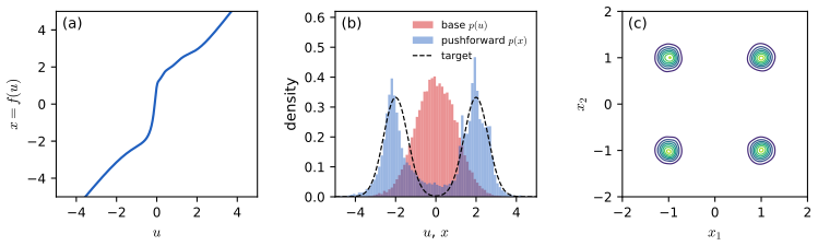
23.2.2.2 Higher-order perturbations. p. 833 Ziegler and Rush (2019) add an inverse-quadratic bump to the affine map, the non-linear squared flow (NLSq): \[ h(u;\bm\theta)=au+b+\frac{c}{1+(du+e)^2},\qquad\bm\theta=(a,b,c,d,e)\in\R^5. \tag{23.9} \] With \(c=0\) it is affine. The bump can create several modes (Figure 23.1). It is invertible when \(a>\frac{9}{8\sqrt3}|c|\,d\) with \(d>0\) (the book prints \(cd\) without the absolute value, which is only right for \(c\ge0\)), and the inverse is the real root of a cubic polynomial, which has a closed form.
Filling the gap 23.5: when the NLSq map is invertible, and its inverse p. 833, "under the constraints ... the function becomes invertible"
Proof
The derivative. With \(z=du+e\), \(h'(u)=a-c\,d\,\gamma(z)\) where \(\gamma(z)=\dfrac{2z}{(1+z^2)^2}\).
The extremes of \(\gamma\). \(\gamma'(z)=\dfrac{2(1+z^2)-8z^2}{(1+z^2)^3}=\dfrac{2(1-3z^2)}{(1+z^2)^3}\), which vanishes at \(z=\pm1/\sqrt3\); \(\gamma\) is odd and tends to 0 at \(\pm\infty\), so its maximum is \(\gamma(1/\sqrt3)=\dfrac{2/\sqrt3}{(4/3)^2}=\dfrac{9}{8\sqrt3}\approx0.6495\) and its minimum is the negative of that.
The condition. For \(d>0\), \(z\) runs over all of \(\R\) as \(u\) does, so \(\inf_uh'(u)=a-\frac{9}{8\sqrt3}|c|\,d\), attained at \(z=\operatorname{sign}(c)/\sqrt3\). Hence: if \(a>\frac{9}{8\sqrt3}|c|d\) then \(h'>0\) everywhere, \(h\) is strictly increasing, and since \(h(u)-au-b\) is bounded and \(a>0\), \(h(u)\to\pm\infty\) as \(u\to\pm\infty\); by continuity \(h\) is a bijection of \(\R\) with a differentiable inverse. If \(a<\frac{9}{8\sqrt3}|c|d\), \(h'<0\) on an interval, so \(h\) is not injective (it goes up, down, then up). On the boundary \(h\) is still a bijection, but \(h'\) vanishes at one point, where the inverse is not differentiable and the induced density is infinite. For \(c<0\) the printed condition \(a>\frac{9}{8\sqrt3}cd\) is satisfied by every positive \(a\), yet \(a=1\), \(c=-2\), \(d=1\) gives \(\min h'=1-1.299=-0.299<0\): the absolute value is needed.
The inverse is a cubic root. To solve \(h(u)=x\), put \(z=du+e\), \(u=(z-e)/d\). Then \(au+b-x=pz+q\) with \(p=a/d\), \(q=b-x-ae/d\), and multiplying \(pz+q+c/(1+z^2)=0\) by \(1+z^2>0\) gives
\[ pz^3+qz^2+pz+(q+c)=0, \]
a cubic, not a quadratic. Its real roots are exactly the solutions of \(h(u)=x\), because the factor \(1+z^2\) never vanishes. When \(h\) is strictly increasing there is exactly one, and it is simple (at a root the derivative of the cubic is \(h_z(z)(1+z^2)\ne0\)), so the other two roots are complex conjugates and Cardano's formula gives the real one: dividing by \(p\) and substituting \(z=t-q/(3p)\) yields \(t^3+Pt+Q=0\) with discriminant \((Q/2)^2+(P/3)^3>0\) and \(t=\sqrt[3]{-Q/2+\sqrt{(Q/2)^2+(P/3)^3}}+\sqrt[3]{-Q/2-\sqrt{(Q/2)^2+(P/3)^3}}\). The code's nlsq_inverse implements this; on random invertible maps it agrees with bisection to better than \(10^{-8}\). \(\square\)
23.2.2.3 Combinations of strictly monotonic scalar functions. pp. 833–834 Strictly increasing functions are closed under conical combinations with a bias, \(a_1h_1+\dots+a_Kh_K+b\) with \(a_k>0\), and under composition. Starting from strictly increasing activations such as the logistic sigmoid and alternating the two operations gives an MLP with positive weights (Huang et al., 2018). The derivative comes from automatic differentiation; the inverse has no closed form but can be found by bisection.
Filling the gap 23.6: monotone networks, their range, and bisection p. 834
Proof
Closure. If \(u<u'\) then \(h_k(u)<h_k(u')\) for each \(k\), and multiplying by \(a_k>0\) and summing keeps the strict inequality. For a composition, \(h_K(u)<h_K(u')\) implies \(h_{K-1}(h_K(u))<h_{K-1}(h_K(u'))\), and so on. A hidden unit \(\sigma(\sum_jw_{ij}h_j(u)+c_i)\) with \(w_{ij}>0\) is a strictly increasing activation of a conical combination, so by induction over layers every unit of a positive-weight MLP, and its output, is strictly increasing in \(u\).
The range. A strictly increasing continuous function is a bijection from \(\R\) onto its range, an open interval. With bounded activations (sigmoid, tanh) that interval is bounded, so the network is not a bijection of \(\R\). Practical designs fix this by ending with an unbounded strictly increasing map (an inverse sigmoid, as in neural autoregressive flows, maps \((0,1)\) onto \(\R\)) or by adding a positive linear term \(\varepsilon u\), as in the code (monotone_sigmoid_mix).
Bisection. If \(h\) is continuous and strictly increasing and \(h(\ell)\le x\le h(r)\), the unique root of \(h(u)=x\) lies in \([\ell,r]\); halving the bracket and keeping the half whose endpoint values straddle \(x\) keeps the root inside, so after \(n\) steps the midpoint is within \((r-\ell)/2^{n+1}\) of it. A tolerance \(\epsilon\) needs \(\lceil\log_2((r-\ell)/\epsilon)\rceil\) evaluations of \(h\), about 50 for \(r-\ell=100\) and \(\epsilon=10^{-13}\), and all coordinates of a batch can be bisected in parallel. The derivative of the inverse needed for the density is \((h^{-1})'(x)=1/h'(h^{-1}(x))\), by differentiating \(h(h^{-1}(x))=x\). \(\square\)
23.2.2.4 Scalar bijections from integration. p. 834 Another route is to parameterise a positive derivative and integrate it: \[ h(u)=\int_0^uh'(t)\,\d t+b. \tag{23.10} \] Unconstrained monotonic neural networks (Wehenkel and Louppe, 2019) take \(h'\) to be a network whose output is made positive by an ELU shifted up by 1, and integrate numerically. Jaini, Selby and Yu (2019) take a sum of squares of polynomials, which integrates in closed form: \[ h'(u)=\sum_{k=1}^K\Big(\sum_{\ell=0}^La_{k\ell}u^\ell\Big)^2, \tag{23.11} \] a non-negative polynomial of degree \(2L\), so \(h\) is an increasing polynomial of degree \(2L+1\) (affine when \(L=0\)). The derivative is read off; the inverse again needs bisection.
Filling the gap 23.7: when integration gives a bijection, and why sums of squares lose nothing p. 834
Proof
Strict monotonicity. If \(h'\) is continuous, non-negative, and vanishes at most at isolated points, then for \(u<u'\), \(h(u')-h(u)=\int_u^{u'}h'(t)\,\d t>0\) because the integrand is positive on a subinterval. A non-negative polynomial that is not identically zero has finitely many zeros, so (23.11) gives a strictly increasing \(h\) unless all \(a_{k\ell}=0\).
Range. For (23.11), if some \(a_{kL}\ne0\) the leading coefficient of \(h'\) is \(\sum_ka_{kL}^2>0\), so \(h\) has odd degree \(2L+1\) with a positive leading coefficient and tends to \(\pm\infty\) at \(\pm\infty\): a bijection of \(\R\). Explicitly, \(h(u)=b+\sum_k\sum_{\ell,m}a_{k\ell}a_{km}u^{\ell+m+1}/(\ell+m+1)\). For the ELU construction, \(h'(t)=\mathrm{ELU}(n(t))+1>0\), but \(\mathrm{ELU}(s)+1=e^s\) for \(s<0\) can decay to zero fast enough that \(\int_0^\infty h'\) is finite; the range is then a bounded interval and the same caution as in gap 23.6 applies.
Zeros of \(h'\). At a zero \(u_0\) of \(h'\) (possible in (23.11), e.g. \(h'(u)=u^2\)), \(h\) is still a bijection, but its inverse is not differentiable at \(h(u_0)\) and the induced density \(p_u(u_0)/h'(u_0)\) is infinite there. So strictly the map is a homeomorphism rather than a diffeomorphism; in practice parameters with an exact zero have probability zero under training.
No loss of generality with \(K=2\). Every non-negative univariate polynomial is a sum of two squares of polynomials: its real roots have even multiplicity (it would change sign otherwise), so it factors as \(c\,r(u)^2\prod_j|u-z_j|^2\) over pairs of complex-conjugate roots, with \(c>0\); each factor \(|u-z_j|^2=(u-\Re z_j)^2+(\Im z_j)^2\) is a sum of two squares, and products of sums of two squares are sums of two squares, \((a^2+b^2)(c^2+d^2)=(ac-bd)^2+(ad+bc)^2\). So (23.11) with \(K=2\) describes every non-negative polynomial of degree \(2L\). \(\square\)
23.2.2.5 Splines. pp. 834–835 A monotone spline is defined by \(K+1\) knots \((u_k,x_k)\) with \(u_{k-1}<u_k\), \(x_{k-1}<x_k\), and an increasing interpolant on each bin. Linear interpolation (Müller et al., 2019) has a discontinuous derivative; quadratic interpolation makes it continuous; cubic (Durkan et al., 2019a), linear-rational (Dolatabadi et al., 2020) and rational-quadratic (Durkan et al., 2019b) interpolants let the derivatives at the knots be free parameters. Low-degree pieces invert analytically: find the bin by binary search, then solve a low-degree equation. The rational-quadratic spline used in Figure 23.3 is worked out next.
Filling the gap 23.8: the rational-quadratic spline: formula, monotonicity, smoothness and closed-form inverse p. 835, "see references above for details"
Proof
Definition. Bin \(k\) maps \([u_k,u_{k+1}]\) onto \([x_k,x_{k+1}]\). Let \(w_k=u_{k+1}-u_k\), \(h_k=x_{k+1}-x_k\), \(s_k=h_k/w_k\) (the bin's slope), \(\delta_k,\delta_{k+1}>0\) the derivatives at the knots, and \(\xi=(u-u_k)/w_k\in[0,1]\). Durkan et al. (2019b) set \[ g(\xi)=x_k+\frac{h_k\big[s_k\xi^2+\delta_k\xi(1-\xi)\big]}{s_k+(\delta_{k+1}+\delta_k-2s_k)\,\xi(1-\xi)}. \] At \(\xi=0\) this is \(x_k\), at \(\xi=1\) it is \(x_k+h_ks_k/s_k=x_{k+1}\): the spline interpolates the knots and is continuous. Outside \([u_0,u_K]\) the identity is used, with \(\delta_0=\delta_K=1\).
The denominator is positive. Write it as \(s_k(1-2\xi(1-\xi))+(\delta_k+\delta_{k+1})\xi(1-\xi)=s_k(\xi^2+(1-\xi)^2)+(\delta_k+\delta_{k+1})\xi(1-\xi)\), a sum of non-negative terms that are not both zero on \([0,1]\).
The derivative. Let \(n(\xi)=s_k\xi^2+\delta_k\xi(1-\xi)\) and \(m(\xi)\) the denominator, \(\Delta=\delta_{k+1}+\delta_k-2s_k\). Then \(n'=2s_k\xi+\delta_k(1-2\xi)\), \(m'=\Delta(1-2\xi)\), and a direct expansion gives \[ n'm-nm'=s_k\big[\delta_{k+1}\xi^2+2s_k\xi(1-\xi)+\delta_k(1-\xi)^2\big]. \] (Collect powers of \(\xi\): the \(\xi^0\) coefficient is \(\delta_ks_k\); the \(\xi^1\) coefficient is \(2s_k^2-2\delta_ks_k\); the \(\xi^2\) coefficient is \(s_k(\delta_{k+1}+\delta_k-2s_k)\); the higher powers cancel; this matches the right side.) Since \(\d\xi/\d u=1/w_k\) and \(h_k/w_k=s_k\), \[ \frac{\d x}{\d u}=\frac{s_k^2\big[\delta_{k+1}\xi^2+2s_k\xi(1-\xi)+\delta_k(1-\xi)^2\big]}{\big[s_k+\Delta\,\xi(1-\xi)\big]^2}>0, \] positive because every term of the numerator is non-negative and they do not all vanish. So the spline is strictly increasing. At \(\xi=0\) the derivative is \(s_k^2\delta_k/s_k^2=\delta_k\) and at \(\xi=1\) it is \(\delta_{k+1}\): adjacent bins share the knot derivative, so the derivative is continuous, and with \(\delta_0=\delta_K=1\) it joins the identity tails continuously.
The inverse. Given \(x\in[x_k,x_{k+1}]\) (bin found by binary search over the \(x_k\)), set \(g(\xi)=x\) and multiply by \(m(\xi)\): \(h_kn(\xi)-(x-x_k)m(\xi)=0\), that is \(a\xi^2+b\xi+c=0\) with \[ a=h_k(s_k-\delta_k)+(x-x_k)\Delta,\qquad b=h_k\delta_k-(x-x_k)\Delta,\qquad c=-s_k(x-x_k). \] Because \(h_kn-(x-x_k)m=m(\xi)\,(g(\xi)-x)\) and \(m>0\), the quadratic has the sign of \(g(\xi)-x\) on \([0,1]\): non-positive at 0, non-negative at 1, with exactly one root in \([0,1]\) by monotonicity. If \(a>0\) that root is the larger root; if \(a<0\) the parabola opens downwards and it is the smaller one; in both cases it equals \((-b+\sqrt{b^2-4ac})/(2a)\), which after multiplying top and bottom by \(-b-\sqrt{b^2-4ac}\) is \[ \xi=\frac{2c}{-b-\sqrt{b^2-4ac}}. \] This form is also correct when \(a=0\) (then \(b>0\) and \(\xi=-c/b\)), and it avoids the cancellation of the textbook formula. Numerically, forward and inverse undo each other to \(10^{-12}\), and the derivative formula matches finite differences. \(\square\)
23.2.3 Coupling flows
pp. 835–836 Split \(\bm u=(\bm u^A,\bm u^B)\in\R^d\times\R^{D-d}\) and let \(\hat{\bm f}(\cdot;\bm\theta)\) be a bijection of \(\R^d\). The coupling layer (Dinh, Krueger and Bengio, 2015; Dinh, Sohl-Dickstein and Bengio, 2017) is \[ \bm x^A=\hat{\bm f}(\bm u^A;\Theta(\bm u^B)), \tag{23.12} \] \[ \bm x^B=\bm u^B, \tag{23.13} \] where the conditioner \(\Theta\) is any function, typically a deep network (MLP, CNN, ResNet). Its inverse is \[ \bm u^A=\hat{\bm f}^{-1}(\bm x^A;\Theta(\bm x^B)), \tag{23.14} \] \[ \bm u^B=\bm x^B, \tag{23.15} \] and its Jacobian is block triangular, \[ \J(\bm f)=\begin{pmatrix}\partial\bm x^A/\partial\bm u^A&\partial\bm x^A/\partial\bm u^B\\ \partial\bm x^B/\partial\bm u^A&\partial\bm x^B/\partial\bm u^B\end{pmatrix}=\begin{pmatrix}\J(\hat{\bm f})&\partial\bm x^A/\partial\bm u^B\\ \bm 0&\I\end{pmatrix}, \tag{23.16} \] so \(\det\J(\bm f)=\det\J(\hat{\bm f})\). Usually \(\hat{\bm f}\) is elementwise, \[ \hat{\bm f}(\bm u^A;\bm\theta)=\big(h(u^A_1;\bm\theta_1),\dots,h(u^A_d;\bm\theta_d)\big), \tag{23.17} \] with any scalar bijection of Section 23.2.2 (affine: real NVP; monotone MLP; spline: neural spline flows). Partitions alternate between layers (halves, or a checkerboard for images) so that every variable gets transformed. With a binary mask \(\bm b\) (1 = passed through), \[ \bm x=\bm b\odot\bm u+(\bm1-\bm b)\odot\hat{\bm f}(\bm u;\Theta(\bm b\odot\bm u)). \tag{23.18} \]
Filling the gap 23.9: the coupling layer is invertible, and its determinant ignores the conditioner p. 836, (23.14)–(23.18)
Proof
Inverse. Given \(\bm x\), (23.13) returns \(\bm u^B=\bm x^B\) at once; the parameters \(\bm\theta=\Theta(\bm u^B)=\Theta(\bm x^B)\) are therefore computable from \(\bm x\) alone, and \(\bm u^A=\hat{\bm f}^{-1}(\bm x^A;\bm\theta)\) because \(\hat{\bm f}(\cdot;\bm\theta)\) is a bijection. The conditioner itself is never inverted, which is why it can be an arbitrary network.
Determinant. \(\bm x^B\) does not depend on \(\bm u^A\), so the lower-left block of (23.16) is zero, and \(\partial\bm x^B/\partial\bm u^B=\I\). For a block upper-triangular matrix, \(\det\begin{pmatrix}\bm P&\bm Q\\\bm0&\bm S\end{pmatrix}=\det\bm P\det\bm S\) (factor it as \(\begin{pmatrix}\bm P&\bm0\\\bm0&\I\end{pmatrix}\begin{pmatrix}\I&\bm Q\\\bm0&\bm S\end{pmatrix}\) when \(\bm P\) is invertible, and expand the second factor along its first columns). So \(\det\J(\bm f)=\det\J(\hat{\bm f})\cdot1\); the possibly huge block \(\partial\bm x^A/\partial\bm u^B\), which involves the derivative of the network, never has to be computed. With (23.17), \(\det\J(\hat{\bm f})=\prod_{i\le d}h'(u^A_i;\bm\theta_i)\).
The masked form. In (23.18), coordinate \(i\) with \(b_i=1\) is copied; coordinate \(i\) with \(b_i=0\) becomes \(h(u_i;\bm\theta_i(\bm b\odot\bm u))\), which depends on \(u_i\) only through \(h\), and on the copied coordinates through \(\bm\theta_i\) (the factor \(\bm b\odot\bm u\) blocks every transformed coordinate from the conditioner). Reordering the coordinates to put the transformed ones first gives exactly (23.16), so \(\det\J=\prod_{i:b_i=0}h'(u_i;\bm\theta_i)\). The affine case is Result 18.2 of the deep-learning course. \(\square\)
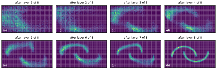
The book fits a masked coupling flow with rational-quadratic splines to the two moons and shows the samples after each layer (Figure 23.3). My version has eight layers that alternate the transformed coordinate, splines with \(K=8\) bins on \([-4,4]\) (identity outside), and conditioners with two hidden layers of 64 units, trained by maximum likelihood (2 500 Adam steps, batches of 256, about 2.5 minutes on a CPU).
23.2.4 Autoregressive flows
pp. 836–838 An autoregressive bijection computes the outputs one at a time, \[ x_i=h(u_i;\Theta_i(\bm x_{1:i-1})),\qquad i=1,\dots,D, \tag{23.19} \] with a scalar bijection \(h\) and conditioners \(\Theta_i\) (arbitrary functions, often networks). Its inverse is \[ u_i=h^{-1}(x_i;\Theta_i(\bm x_{1:i-1})),\qquad i=1,\dots,D, \tag{23.20} \] and its Jacobian is triangular, so \[ \det\J(\bm f)=\prod_{i=1}^D\frac{\partial x_i}{\partial u_i}=\prod_{i=1}^D\frac{\d h}{\d u_i}, \tag{23.21} \] in \(O(D)\) time. The two directions cost differently: \(\bm f\) is sequential (\(x_i\) needs \(\bm x_{1:i-1}\)), while \(\bm f^{-1}\) is parallel (all of \(\bm x\) is known, so every \(u_i\) can be computed at once).
Filling the gap 23.10: invertibility, the triangular Jacobian, and the cost of each direction p. 837, (23.19)–(23.21)
Proof
Invertibility. Given \(\bm x\), every conditioner input \(\bm x_{1:i-1}\) is known, so (23.20) gives each \(u_i\) uniquely; conversely, given \(\bm u\), (23.19) defines \(x_1,x_2,\dots\) in turn. The two maps compose to the identity in both orders, so \(\bm f\) is a bijection.
Triangular Jacobian. By induction on \(i\), \(x_i\) is a function of \(\bm u_{1:i}\) only: \(x_1=h(u_1;\Theta_1)\) depends on \(u_1\); if \(\bm x_{1:i-1}\) depends on \(\bm u_{1:i-1}\), then \(x_i=h(u_i;\Theta_i(\bm x_{1:i-1}))\) depends on \(\bm u_{1:i}\). Hence \(\partial x_i/\partial u_j=0\) for \(j>i\), the Jacobian is lower triangular, and its determinant is the product of the diagonal entries, \(\partial x_i/\partial u_i=h'(u_i;\Theta_i(\bm x_{1:i-1}))\) (the conditioner's input does not involve \(u_i\)).
Cost. With a single network that outputs all \(\Theta_i\) at once (Section 23.2.4.2), the inverse needs one network pass; the forward map needs \(D\) passes, one per coordinate, since \(\Theta_i\) cannot be computed before \(x_{i-1}\) is known. The deep-learning course tabulates the same trade-off in Result 18.3. \(\square\)
23.2.4.1 Affine autoregressive flows. pp. 838–839 With an affine \(h\) parameterised by a log-scale \(\alpha_i\) and a shift \(\mu_i\), \[ x_i=u_i\exp(\alpha_i(\bm x_{1:i-1}))+\mu_i(\bm x_{1:i-1}), \tag{23.22} \] \[ u_i=(x_i-\mu_i(\bm x_{1:i-1}))\exp(-\alpha_i(\bm x_{1:i-1})), \tag{23.23} \] \[ \log|\det\J(\bm f)|=\log\Big|\prod_{i=1}^D\exp(\alpha_i(\bm x_{1:i-1}))\Big|=\sum_{i=1}^D\alpha_i(\bm x_{1:i-1}). \tag{23.24} \] In two dimensions with \(\bm u\sim\N(\bm0,\I)\), \(x_1\) is \(\N(\mu_1,\sigma_1^2)\) with \(\sigma_1=e^{\alpha_1}\), and given \(x_1\), \(x_2\) is Gaussian with mean \(\mu_2(x_1)\) and standard deviation \(\sigma_2(x_1)=e^{\alpha_2(x_1)}\). So one layer always has Gaussian conditionals, \[ p(x_1,x_2)=p(x_1)\,p(x_2\given x_1)=\N(x_1\given\mu_1,\sigma_1^2)\,\N(x_2\given\mu_2(x_1),\sigma_2(x_1)^2), \tag{23.25} \] however flexible \(\mu_2\) and \(\alpha_2\) are, and the same holds in \(D\) dimensions. A cross-shaped density has bimodal conditionals and cannot be fitted by one layer (Figure 23.5(b)); five layers that reverse the order of the variables after each layer fit it (Figure 23.5(c)). A more flexible \(h\) (monotone MLP, spline) is another fix.
Filling the gap 23.11: Gaussian conditionals, why the cross defeats one layer, and what the best single layer is pp. 838–839, (23.25) and "this result generalizes to an arbitrary number of dimensions"
Proof
Gaussian conditionals in \(D\) dimensions. The \(u_i\) are independent \(\N(0,1)\). By the induction of gap 23.10, \(\bm x_{1:i-1}\) is a function of \(\bm u_{1:i-1}\), hence independent of \(u_i\). Conditionally on \(\bm x_{1:i-1}\), (23.22) is an affine function of the independent \(u_i\sim\N(0,1)\) with fixed coefficients, so \(x_i\given\bm x_{1:i-1}\sim\N(\mu_i(\bm x_{1:i-1}),e^{2\alpha_i(\bm x_{1:i-1})})\), and \(p(\bm x)=\prod_i\N(x_i\given\mu_i,e^{2\alpha_i})\).
The cross density. Mine (Figure 23.5(a)) is \(\frac12\N(\bm0,\bm\Sigma_+)+\frac12\N(\bm0,\bm\Sigma_-)\) where \(\bm\Sigma_\pm\) have standard deviations \(s_L=1.5\) along the diagonal \(x_2=\pm x_1\) and \(s_S=0.25\) across it, so \(\bm\Sigma_\pm=\frac12\begin{pmatrix}s_L^2+s_S^2&\pm(s_L^2-s_S^2)\\\pm(s_L^2-s_S^2)&s_L^2+s_S^2\end{pmatrix}\). Both components have the same \(x_1\)-marginal \(\N(0,v)\), \(v=\frac12(s_L^2+s_S^2)\), so the mixture weights do not change on conditioning, and by Gaussian conditioning \[ x_2\given x_1\sim\tfrac12\N(rx_1,\tau^2)+\tfrac12\N(-rx_1,\tau^2),\qquad r=\frac{s_L^2-s_S^2}{s_L^2+s_S^2},\quad\tau^2=\frac{2s_L^2s_S^2}{s_L^2+s_S^2}. \] Here \(r=0.946\) and \(\tau=0.349\). An equal mixture of two Gaussians with common variance is bimodal when the means are more than \(2\tau\) apart, i.e. for \(|x_1|>\tau/r=0.37\). By symmetry the same happens for the other ordering, so no single affine autoregressive layer can represent the cross.
The best single layer. Maximum likelihood minimises \(\Dkl(p\|q)=\Dkl(p(x_1)\|q(x_1))+\E_{p(x_1)}\Dkl(p(x_2\given x_1)\|q(x_2\given x_1))\) (chain rule for KL). The first term is zero for \(q(x_1)=\N(0,v)\), since \(p(x_1)\) is that Gaussian. For each \(x_1\), the Gaussian closest in forward KL to a distribution with mean \(m\) and variance \(s^2\) is \(\N(m,s^2)\) (minimise \(\E[-\log\N(x_2\given\mu,\sigma^2)]=\log\sigma+\frac{s^2+(m-\mu)^2}{2\sigma^2}+\const\)). The conditional above has mean 0 and variance \(r^2x_1^2+\tau^2\), so with unrestricted \(\mu_2,\alpha_2\) the optimum is \[ q^\star(x_1,x_2)=\N(x_1\given0,v)\,\N\big(x_2\given0,r^2x_1^2+\tau^2\big), \] the hourglass of Figure 23.5(b): a Gaussian in \(x_2\) whose spread grows linearly with \(|x_1|\), with its mass along \(x_2=0\) where the cross has little. Its expected log-likelihood under the cross is \(-2.670\) nats, against \(-2.346\) for the cross itself (minus its entropy). On my test set of 2 000 draws, \(q^\star\) scores \(-2.6375\), the trained one-layer flow \(-2.6375\) (it has found this optimum), the five-layer flow \(-2.355\) and the true density \(-2.350\). \(\square\)

23.2.4.2 Masked autoregressive flows. pp. 839–840 Using \(D\) separate networks for the conditioners is wasteful. Instead one network \(\Theta\) outputs \((\bm\theta_1,\dots,\bm\theta_D)\) from \(\bm x\), with connections removed so that \(\bm\theta_i\) depends only on \(\bm x_{1:i-1}\). The masked autoregressive flow (MAF; Papamakarios, Pavlakou and Murray, 2017) is an affine autoregressive flow with permutations whose conditioner is an MLP with each weight matrix multiplied elementwise by a binary mask, built as in MADE (Germain et al., 2015) so that every path from \(x_j\) to \(\bm\theta_i\) with \(j\ge i\) is cut. One masked pass costs the same as an unmasked one and gives all \(\bm\theta_i\): density evaluation is one pass, sampling \(D\) passes. MAF therefore suits density estimation more than generation. (With \(D=2\), as in Figure 23.5, the masked network reduces to a constant for \(\bm\theta_1\) and a network of \(x_1\) for \(\bm\theta_2\), which is how the code writes it.) Why the MADE masks have this property is proved in the deep-learning course, gap 18.5.
23.2.4.3 Inverse autoregressive flows. pp. 840–841 Making the parameters depend on the previous inputs instead, \[ x_i=h(u_i;\Theta_i(\bm u_{1:i-1})),\qquad i=1,\dots,D, \tag{23.26} \] gives an inverse autoregressive bijection, again with triangular Jacobian and \(\det\J(\bm f)=\prod_ih'\). It is (23.20) with \(\bm u\) and \(\bm x\) swapped and \(h\) replaced by \(h^{-1}\): it parameterises the inverse of an autoregressive bijection directly, so the costs swap: sampling is parallel and fast, density evaluation at an arbitrary \(\bm x\) is sequential. IAF (Kingma et al., 2016) uses affine bijections, masked conditioners and permutations, and is exactly the inverse of MAF. Its density is free for its own samples, which is all variational inference needs (Section 23.1.2.2). Parallel WaveNet (van den Oord et al., 2018) trains an IAF student \(p_s\) to mimic a trained WaveNet \(p_t\), whose density is cheap but whose sampling is slow, by minimising \(\Dkl(p_s\|p_t)\).
Filling the gap 23.12: the IAF density of its own samples, and why distillation only needs the cheap directions p. 841
Proof
Density of a sample. To sample, draw \(\bm u\) and compute all \(\Theta_i(\bm u_{1:i-1})\) in one masked pass, then each \(x_i=h(u_i;\Theta_i)\) in parallel. The triangular Jacobian gives \(\log p_x(\bm x)=\log p_u(\bm u)-\sum_i\log h'(u_i;\Theta_i(\bm u_{1:i-1}))\), and every quantity on the right was computed during sampling. For an externally given \(\bm x\), by contrast, \(\bm u\) must be recovered by \(u_i=h^{-1}(x_i;\Theta_i(\bm u_{1:i-1}))\) in sequence, \(D\) passes.
Distillation. \(\Dkl(p_s\|p_t)=\E_{\bm x\sim p_s}[\log p_s(\bm x)-\log p_t(\bm x)]\). An unbiased estimate is the average of \(\log p_s(\bm x_n)-\log p_t(\bm x_n)\) over samples \(\bm x_n=\bm f_s(\bm u_n)\) of the student: the student's term is free by the previous paragraph, and the teacher's term is one parallel (teacher-forced) pass of the autoregressive teacher over the whole sequence. Writing \(\bm x_n=\bm f_s(\bm u_n)\), the gradient with respect to the student's parameters passes through the samples by reparameterisation, exactly as in gap 23.3. Neither slow direction (IAF density at external points, WaveNet sampling) is ever used. The reverse KL is mode-seeking, which is why practical systems add further losses to keep the student from dropping parts of the teacher's distribution. \(\square\)
23.2.4.4 Connection with autoregressive models. pp. 841–842 A continuous autoregressive model \[ p(\bm x)=\prod_{i=1}^Dp_i(x_i\given\bm\theta_i),\qquad\bm\theta_i=\Theta_i(\bm x_{1:i-1}), \tag{23.27} \] (for example with a mixture of one-dimensional Gaussians for each conditional) is sampled one coordinate at a time, \[ x_i\sim p_i(x_i\given\Theta_i(\bm x_{1:i-1})),\qquad i=1,\dots,D, \tag{23.28} \] and by inverse-cdf sampling \[ x_i=\CDF_i^{-1}(u_i\given\Theta_i(\bm x_{1:i-1})),\qquad u_i\sim\U(0,1). \tag{23.29} \] This is (23.19) with a uniform base on \([0,1]^D\) and the inverse conditional cdfs as scalar bijections: every continuous autoregressive model is a one-layer autoregressive flow, and stacking several keeps the density exact.
Filling the gap 23.13: the flow density of an autoregressive model is the model's own density p. 842, (23.29)
Proof
Assume each conditional density \(p_i(\cdot\given\bm\theta)\) is continuous and positive, so \(\CDF_i(\cdot\given\bm\theta)\) is a \(C^1\) strictly increasing bijection from \(\R\) onto \((0,1)\) with derivative \(p_i\) (inverse-cdf sampling itself is proved for any cdf in gap 11.2). Then \(h(u;\bm\theta)=\CDF_i^{-1}(u\given\bm\theta)\) is a scalar bijection from \((0,1)\) onto \(\R\) with \(h'(u)=1/p_i(h(u)\given\bm\theta)\), by the inverse-function rule. By (23.21), \(|\det\J(\bm f)(\bm u)|=\prod_i1/p_i(x_i\given\bm\theta_i)\), and the uniform base has \(p_u=1\) on \((0,1)^D\). So (23.2) gives
\[ p_x(\bm x)=1\cdot\prod_{i=1}^Dp_i(x_i\given\Theta_i(\bm x_{1:i-1})), \]
which is (23.27): the flow view changes nothing about the model, only how it is written. For a mixture of Gaussians the cdf has no closed-form inverse, so sampling uses bisection (gap 23.6), while the density needs only the cdf: the inverse direction (23.20) is \(u_i=\CDF_i(x_i\given\cdot)\), in closed form. The identity is confirmed numerically for a two-dimensional model whose first conditional is a Gaussian mixture (the flow is built by ar_as_flow). \(\square\)
23.2.5 Residual flows
p. 842 A residual connection is \(\bm f(\bm u)=\bm u+\bm F(\bm u)\), with residual block \(\bm F:\R^D\to\R^D\). It is not invertible in general; two kinds of block make it so.
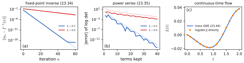
23.2.5.1 Contractive residual blocks. pp. 842–843 Let \(\bm F\) be a contraction: for some \(0\le L<1\) and all \(\bm u_1,\bm u_2\), \[ \|\bm F(\bm u_1)-\bm F(\bm u_2)\|\le L\|\bm u_1-\bm u_2\|. \tag{23.30} \] For a target \(\bm x\), the map \(\bm g(\bm u)=\bm x-\bm F(\bm u)\) is then a contraction, so by Banach's theorem it has a unique fixed point \(\bm u^*\), and \[ \bm u^*=\bm x-\bm F(\bm u^*) \tag{23.31} \] \[ \Rightarrow\ \bm u^*+\bm F(\bm u^*)=\bm x \tag{23.32} \] \[ \Rightarrow\ \bm f(\bm u^*)=\bm x, \tag{23.33} \] so \(\bm u^*=\bm f^{-1}(\bm x)\). The invertible ResNet (iResNet; Behrmann et al., 2019) makes its convolutional blocks contractive with spectral normalisation (Miyato et al., 2018) and activations of slope at most 1, since Lipschitz constants multiply under composition. The inverse is computed by iterating \[ \bm u_n=\bm g(\bm u_{n-1})=\bm x-\bm F(\bm u_{n-1}), \tag{23.34} \] which converges at rate \(O(L^n)\) from any start (\(\bm u_0=\bm x\) is convenient). The log-determinant has no closed form, but \[ \log|\det\J(\bm f)|=\log|\det(\I+\J(\bm F))|=\sum_{k=1}^\infty\frac{(-1)^{k+1}}{k}\Tr\big(\J(\bm F)^k\big), \tag{23.35} \] convergent because \(\|\J(\bm F)\|\le L<1\), and each trace can be estimated with vector-Jacobian products by Hutchinson's estimator, \[ \Tr\big(\J(\bm F)^k\big)\approx\bm v^\T\J(\bm F)^k\bm v, \tag{23.36} \] for \(\bm v\) with zero mean and identity covariance. Truncating the series gives a biased estimate (Behrmann et al., 2019); the Russian-roulette estimator (Chen et al., 2019) is unbiased.
Filling the gap 23.14: contractive residual flows: invertibility, convergence, the series and its two estimators pp. 842–843, (23.30)–(23.36)
Proof
Invertibility (23.31)–(23.33). \(\|\bm g(\bm u_1)-\bm g(\bm u_2)\|=\|\bm F(\bm u_1)-\bm F(\bm u_2)\|\le L\|\bm u_1-\bm u_2\|\), so \(\bm g\) is a contraction of the complete space \(\R^D\) and has exactly one fixed point (Banach). Existence gives surjectivity of \(\bm f\); for injectivity, if \(\bm f(\bm u_1)=\bm f(\bm u_2)=\bm x\) then both are fixed points of the same \(\bm g\), hence equal. Quantitatively, \(\|\bm f(\bm u_1)-\bm f(\bm u_2)\|\ge\|\bm u_1-\bm u_2\|-\|\bm F(\bm u_1)-\bm F(\bm u_2)\|\ge(1-L)\|\bm u_1-\bm u_2\|\), and similarly \(\le(1+L)\|\bm u_1-\bm u_2\|\): \(\bm f\) is bi-Lipschitz and \(\bm f^{-1}\) has Lipschitz constant at most \(1/(1-L)\).
Rate of (23.34). \(\|\bm u_n-\bm u^*\|=\|\bm g(\bm u_{n-1})-\bm g(\bm u^*)\|\le L\|\bm u_{n-1}-\bm u^*\|\le\dots\le L^n\|\bm u_0-\bm u^*\|\). A bound that uses only computed quantities follows from the triangle inequality, \(\|\bm u_0-\bm u^*\|\le\|\bm u_0-\bm u_1\|+L\|\bm u_0-\bm u^*\|\), so \(\|\bm u_n-\bm u^*\|\le\frac{L^n}{1-L}\|\bm u_1-\bm u_0\|\). With \(\bm u_0=\bm x\), \(\|\bm u_0-\bm u^*\|=\|\bm F(\bm u^*)\|\), small when the block is small.
The Jacobian. If \(\bm F\) is differentiable, (23.30) gives \(\|\J(\bm F)(\bm u)\bm e\|=\lim_{t\to0}\|\bm F(\bm u+t\bm e)-\bm F(\bm u)\|/t\le L\|\bm e\|\), so the spectral norm of \(\bm A=\J(\bm F)(\bm u)\) is at most \(L\), and every eigenvalue satisfies \(|\lambda|\le L<1\). The eigenvalues of \(\I+\bm A\) are \(1+\lambda\): real ones are positive, complex ones come in conjugate pairs with product \(|1+\lambda|^2>0\). So \(\det(\I+\bm A)>0\), \(|\det|\) can be dropped, and \(\bm f\) is a diffeomorphism.
The series (23.35). For \(|\lambda|<1\), \(\log(1+\lambda)=\sum_{k\ge1}(-1)^{k+1}\lambda^k/k\) (principal branch). Summing over the eigenvalues (with multiplicity), \(\sum_i\log(1+\lambda_i)\) is real (conjugate pairs contribute conjugate terms) and its exponential is \(\prod_i(1+\lambda_i)=\det(\I+\bm A)\); along the path \(t\bm A\), \(t\in[0,1]\), both it and \(\log\det(\I+t\bm A)\) are continuous and agree at \(t=0\), so they agree at \(t=1\). Exchanging the two sums (absolutely convergent) and using \(\sum_i\lambda_i^k=\Tr(\bm A^k)\) gives (23.35). Since \(|\Tr(\bm A^k)|\le D\,L^k\), keeping \(n\) terms leaves an error of at most \[ \sum_{k>n}\frac{D\,L^k}{k}\le\frac{D\,L^{n+1}}{(n+1)(1-L)}. \] Figure 23.x1(b) shows the actual error against this bound: at \(L=0.9\) 43 terms are needed for an error below \(10^{-3}\), at \(L=0.5\) only 8.
Hutchinson (23.36). \(\E[\bm v^\T\bm M\bm v]=\E\Tr(\bm M\bm v\bm v^\T)=\Tr(\bm M\,\E[\bm v\bm v^\T])=\Tr\bm M\) whenever \(\E[\bm v\bm v^\T]=\I\) (a zero mean is not needed); \(\bm v^\T\bm A^k\bm v\) is computed with \(k\) Jacobian-vector products and never forms \(\bm A\). Variances are in Result 18.7. The truncated series with Hutchinson traces is unbiased for the truncated sum, hence biased for the log-determinant by the remainder above.
Russian roulette. Let \(a_k=(-1)^{k+1}\Tr(\bm A^k)/k\) and let \(N\ge1\) be a random integer, independent of everything else, with \(q_k=\Pr(N\ge k)>0\) for all \(k\). The estimator \(\hat S=\sum_{k=1}^Na_k/q_k\) satisfies \[ \E\hat S=\E\sum_{k=1}^\infty\frac{a_k}{q_k}\mathbb 1\{N\ge k\}=\sum_{k=1}^\infty\frac{a_k}{q_k}\Pr(N\ge k)=\sum_{k=1}^\infty a_k, \] where the exchange of \(\E\) and \(\sum\) is justified by Fubini's theorem, because \(\E\sum_k|a_k|\mathbb 1\{N\ge k\}/q_k=\sum_k|a_k|<\infty\). So it is unbiased with a finite expected number of terms \(\E N=\sum_kq_k\). Its variance, \(\sum_{k,j}a_ka_j\,(q_{\max(k,j)}/(q_kq_j))-(\sum a_k)^2\), is finite when \(q_k\) decays more slowly than \(a_k^2\); for a geometric \(N\) with \(q_k=p^{k-1}\) this needs \(L^2<p\). A numerical test on a \(4\times4\) contraction confirms the unbiasedness. \(\square\)
23.2.5.2 Residual blocks with low-rank Jacobian. pp. 843–844 For a \(D\times M\) matrix \(\bm A\) and an \(M\times D\) matrix \(\bm B\), the Weinstein–Aronszajn identity (a special case of the matrix determinant lemma) states \[ \det(\I_D+\bm A\bm B)=\det(\I_M+\bm B\bm A), \tag{23.37} \] turning an \(O(D^3)\) determinant into an \(O(M^3)\) one. If the residual block has a bottleneck, \(\bm F=\bm F_2\circ\bm F_1\) with \(\bm F_1:\R^D\to\R^M\), \(\bm F_2:\R^M\to\R^D\), \(M\ll D\), then \(\J(\bm F)=\J(\bm F_2)\J(\bm F_1)\) and \[ \det\J(\bm f)=\det(\I_D+\J(\bm F))=\det(\I_D+\J(\bm F_2)\J(\bm F_1))=\det(\I_M+\J(\bm F_1)\J(\bm F_2)). \tag{23.38} \] The planar flow (Rezende and Mohamed, 2015) is the case \(M=1\): \[ \bm f(\bm u)=\bm u+\bm v\,\sigma(\bm w^\T\bm u+b), \tag{23.39} \] with \(\bm v,\bm w\in\R^D\), \(b\in\R\), \(\bm F_1(\bm u)=\bm w^\T\bm u+b\), \(\bm F_2(z)=\bm v\sigma(z)\), \(\J(\bm F_1)=\bm w^\T\), \(\J(\bm F_2)=\bm v\sigma'(z)\), so \[ \det\J(\bm f)(\bm u)=1+\bm w^\T\bm v\,\sigma'(\bm w^\T\bm u+b), \tag{23.40} \] in \(O(D)\). Radial flows (Rezende and Mohamed, 2015) and Sylvester flows (van den Berg et al., 2018) are other examples. Invertibility is not automatic and has to be checked case by case; for \(\sigma=\tanh\) the planar flow is invertible when \(\bm w^\T\bm v>-1\).
Filling the gap 23.15: the Weinstein–Aronszajn identity, and exactly when a planar flow is invertible pp. 843–844, (23.37)–(23.40)
Proof
(23.37). Consider the block matrix \(\bm Z=\begin{pmatrix}\I_D&-\bm A\\\bm B&\I_M\end{pmatrix}\). Eliminating with the top-left block, \(\bm Z=\begin{pmatrix}\I_D&\bm0\\\bm B&\I_M\end{pmatrix}\begin{pmatrix}\I_D&-\bm A\\\bm0&\I_M+\bm B\bm A\end{pmatrix}\), so \(\det\bm Z=\det(\I_M+\bm B\bm A)\). Eliminating with the bottom-right block, \(\bm Z=\begin{pmatrix}\I_D+\bm A\bm B&-\bm A\\\bm0&\I_M\end{pmatrix}\begin{pmatrix}\I_D&\bm0\\\bm B&\I_M\end{pmatrix}\), so \(\det\bm Z=\det(\I_D+\bm A\bm B)\). (Multiply out to check both factorisations; the determinant of a block-triangular matrix is the product of the determinants of its diagonal blocks, gap 23.9.) Equating proves the identity. With \(M=1\), \(\bm A=\bm v\sigma'\), \(\bm B=\bm w^\T\), it gives (23.40).
Reduction to one dimension. Let \(\alpha=\bm w^\T\bm u\) and \(\beta=\bm w^\T\bm v\). Taking the inner product of \(\bm x=\bm u+\bm v\tanh(\bm w^\T\bm u+b)\) with \(\bm w\), \[ \bm w^\T\bm x=\phi(\alpha),\qquad\phi(\alpha)=\alpha+\beta\tanh(\alpha+b). \] If \(\beta>-1\), \(\bm f\) is a diffeomorphism. \(\phi'(\alpha)=1+\beta\sech^2(\alpha+b)\ge\min(1,1+\beta)>0\) because \(\sech^2\in(0,1]\); and \(\phi(\alpha)\to\pm\infty\) at \(\pm\infty\). So \(\phi\) is a bijection of \(\R\). Given \(\bm x\), the only possible \(\alpha\) is \(\phi^{-1}(\bm w^\T\bm x)\), and then (23.39) forces \(\bm u=\bm x-\bm v\tanh(\alpha+b)\); this \(\bm u\) does satisfy \(\bm w^\T\bm u=\bm w^\T\bm x-\beta\tanh(\alpha+b)=\alpha\), hence \(\bm f(\bm u)=\bm x\). So \(\bm f\) is bijective, its inverse costs one scalar root-find (bisection, gap 23.6), and the determinant (23.40) equals \(\phi'(\alpha)>0\).
If \(\beta<-1\), \(\bm f\) is not injective. \(\phi'(-b)=1+\beta<0\), so \(\phi\) decreases near \(-b\) and there are \(\alpha_1\ne\alpha_2\) with \(\phi(\alpha_1)=\phi(\alpha_2)\). Pick any \(\bm x\) with \(\bm w^\T\bm x=\phi(\alpha_1)\) and set \(\bm u_j=\bm x-\bm v\tanh(\alpha_j+b)\). As above \(\bm w^\T\bm u_j=\alpha_j\), so \(\bm f(\bm u_1)=\bm f(\bm u_2)=\bm x\) with \(\bm u_1\ne\bm u_2\). Moreover (23.40) is negative near the fold, so the formula \(p_u(\bm f^{-1}(\bm x))/|\det\J|\), applied with one preimage, no longer integrates to 1: the planar-flow demonstration shows the lost mass.
The boundary \(\beta=-1\) gives a bijection whose Jacobian is singular on the hyperplane \(\bm w^\T\bm u=-b\), so not a diffeomorphism. Rezende and Mohamed (2015) enforce \(\beta>-1\) by replacing \(\bm v\) with \(\hat{\bm v}=\bm v+[m(\bm w^\T\bm v)-\bm w^\T\bm v]\bm w/\|\bm w\|^2\), \(m(s)=-1+\log(1+e^s)\), so that \(\bm w^\T\hat{\bm v}=m(\bm w^\T\bm v)>-1\). Because the inverse needs a root-find and the density at an external point needs the inverse of every layer, planar flows are used for variational posteriors (forward direction only) rather than for density estimation. \(\square\)
23.2.6 Continuous-time flows
pp. 844–846 Instead of a sequence of maps, transform the input continuously: \(\bm x(t)\), \(t\in[0,T]\), solves \[ \frac{\d\bm x}{\d t}(t)=\bm F(\bm x(t),t), \tag{23.41} \] with a time-dependent vector field \(\bm F:\R^D\times[0,T]\to\R^D\) (the velocity of a particle at \(\bm x(t)\)), and the flow \(\bm f\) maps \(\bm x(0)=\bm x_0\) to \(\bm x(T)\). It is a well-defined bijection if \(\bm F(\cdot,t)\) is Lipschitz with a constant that does not depend on \(t\), \[ \|\bm F(\bm x_1,t)-\bm F(\bm x_2,t)\|\le L\|\bm x_1-\bm x_2\|, \tag{23.42} \] by the Picard–Lindelöf theorem. Euler's method with step \(\epsilon\), \[ \bm x(t+\epsilon)=\bm x(t)+\epsilon\bm F(\bm x(t),t), \tag{23.43} \] is a residual connection with block \(\epsilon\bm F(\cdot,t)\), so an ODE solver is a residual network with \(O(T/\epsilon)\) layers; Runge–Kutta methods, some with adaptive steps, are more accurate. The inverse solves the ODE backwards from \(\bm x(T)\), at the same cost as the forward direction. With \(\bm f_t\) the flow for time \(t\) and \(L(t)=\log|\det\J(\bm f_t)(\bm x_0)|\), \(L(0)=0\) and \[ \frac{\d L}{\d t}(t)=\Tr\big(\J(\bm F(\cdot,t))(\bm x(t))\big), \tag{23.44} \] so \(L(T)\) is computed by solving this ODE together with (23.41) on the extended state \((\bm x,L)\). Neural ODEs (Chen et al., 2018) parameterise \(\bm F\) with a network and obtain gradients by the adjoint method (the deep-learning course derives it in Result 18.4 and Algorithm 18.2); FFJORD (Grathwohl et al., 2019) replaces the trace by Hutchinson's estimator. These models are slow to train; flow matching (Section 25.4.7 of the book) trains continuous-time flows by a simple regression instead.
Filling the gap 23.16: why the flow map is a bijection, a proof of (23.44), and Euler steps as contractive residual blocks pp. 844–845, (23.42)–(23.44), "it can be shown that L satisfies the following ODE"
Proof
Existence, uniqueness, bijectivity. Assume \(\bm F\) is continuous in \((\bm x,t)\) and satisfies (23.42) (continuity in \(t\) is also needed; the book leaves it implicit). Then \(\|\bm F(\bm x,t)\|\le\|\bm F(\bm0,t)\|+L\|\bm x\|\) grows at most linearly, so solutions cannot blow up in finite time, and the global Picard–Lindelöf theorem gives a unique solution on \([0,T]\) for every \(\bm x_0\). Grönwall's inequality applied to two solutions gives \(\|\bm f(\bm x_0)-\bm f(\bm x_0')\|\le e^{LT}\|\bm x_0-\bm x_0'\|\). The time-reversed field \(\bm y'(s)=-\bm F(\bm y(s),T-s)\) satisfies the same conditions; solving it from \(\bm y(0)=\bm x_T\) produces \(\bm x(0)\) with \(\bm f(\bm x(0))=\bm x_T\) (surjectivity), and uniqueness of solutions through the point \((\bm x_T,T)\) gives injectivity. So \(\bm f\) is a bijection whose inverse is the backward solve, bi-Lipschitz with constant \(e^{LT}\).
The trace ODE (23.44). Assume also that \(\bm F\) is \(C^1\) in \(\bm x\). Then \(\bm f_t\) is differentiable in \(\bm x_0\) and \(\bm M(t)=\J(\bm f_t)(\bm x_0)\) solves the variational equation obtained by differentiating (23.41) with respect to \(\bm x_0\): \[ \frac{\d\bm M}{\d t}=\J(\bm F(\cdot,t))(\bm x(t))\,\bm M(t),\qquad\bm M(0)=\I. \] Jacobi's formula for the derivative of a determinant, \(\frac{\d}{\d t}\det\bm M=\det\bm M\,\Tr(\bm M^{-1}\dot{\bm M})\), gives, wherever \(\det\bm M\ne0\), \[ \frac{\d}{\d t}\log\det\bm M(t)=\Tr\big(\bm M^{-1}\J(\bm F)\bm M\big)=\Tr\J(\bm F(\cdot,t))(\bm x(t)), \] by the cyclic property of the trace. The solution \(\det\bm M(t)=\exp\int_0^t\Tr\J(\bm F)\,\d s\) is positive for all \(t\) (Liouville's formula), so the absolute value is harmless and \(L(t)=\int_0^t\Tr\J(\bm F(\cdot,s))(\bm x(s))\,\d s\), which is (23.44) with \(L(0)=0\). The deep-learning course states the same result as the instantaneous change of variables, Result 18.6. Figure 23.x1(c) integrates both \(\bm M(t)\) and \(L(t)\) with a fourth-order Runge–Kutta method and they agree.
Euler steps are contractive residual blocks. The block \(\epsilon\bm F(\cdot,t)\) of (23.43) has Lipschitz constant \(\epsilon L\). For \(\epsilon<1/L\) it is a contraction, so each Euler step is invertible by gap 23.14, with log-determinant \(\sum_k(-1)^{k+1}\epsilon^k\Tr(\J(\bm F)^k)/k=\epsilon\Tr\J(\bm F)+O(\epsilon^2)\). Summing over the \(T/\epsilon\) steps and letting \(\epsilon\to0\) recovers \(\int_0^T\Tr\J(\bm F)\,\d t\): a second route to (23.44), and the precise sense in which a continuous-time flow is the limit of residual flows. \(\square\)
23.3 Applications
23.3.1 Density estimation
p. 846 Flows give exact, possibly multimodal densities (Figure 23.3). Early examples are Gaussianization (Chen and Gopinath, 2000) for low-dimensional densities; Tabak and Vanden-Eijnden (2010) and Tabak and Turner (2013) introduced flows as compositions of simple maps and the name "normalizing flow"; Rippel and Adams (2013) used neural networks; NICE (Dinh, Krueger and Bengio, 2015) and real NVP (Dinh, Sohl-Dickstein and Bengio, 2017; "non-volume preserving", since the Jacobian determinant is not 1) followed, and MAF (Section 23.2.4.2) improved unconditional and conditional density estimation. Hybrid models (Nalisnick et al., 2019) model \(p(\bm x,y)\) with a flow for \(\bm x\) and a classifier on its latent representation; the joint density costs one forward pass and serves anomaly detection, semi-supervised learning and selective classification, and residual flows improve them further (Chen et al., 2019). Flows fitted to embeddings are also used for anomaly detection.
See also: density estimation as a goal of generative modelling (Chapter 20).
23.3.2 Generative modeling
pp. 846–847 Flows generate images (Glow, residual flows), video, audio, text, graphs and point clouds. For audio, parallel WaveNet distils WaveNet into an IAF (Section 23.2.4.3), and WaveFlow (Ping, Peng and Zhao, 2020) and FloWaveNet (Kim et al., 2019) speed up WaveNet with coupling layers. For text, discrete flows act on a vocabulary (Tran et al., 2019), or flows model a continuous latent space of a model with discrete observations (Ziegler and Rush, 2019).
23.3.3 Inference
p. 847 Rezende and Mohamed (2015) popularised flows as variational posteriors in latent variable models (Section 23.1.2.2); Householder, inverse autoregressive, multiplicative and Sylvester flows extended this, also to posteriors over Bayesian neural network weights. Flows serve as proposals for importance sampling (neural importance sampling; Boltzmann generators), and as reparameterisations for HMC (Hoffman et al., 2019): running Hamiltonian Monte Carlo in the base space of a flow fitted to the posterior makes the target close to a standard Gaussian. In simulation-based inference, where the likelihood cannot be evaluated but the model can be simulated, a flow trained on simulations approximates the posterior or the likelihood, and can guide further simulations; this has been used in cosmology and computational neuroscience.
See also: flow posteriors in Chapter 10 and inverse-cdf sampling in Chapter 11.
Practice problems
The book has no end-of-chapter exercises for Chapter 23, so here are three short problems of my own, with complete solutions (hidden).
Practice problem 23.1 (an NLSq map). Take \(a=d=1\), \(b=e=0\) in (23.9). (a) For which \(c\) is \(h\) invertible? (b) With \(c=1\), find \(h^{-1}(1)\) by solving the cubic of gap 23.5, and the density at \(x=1\) of \(h(u)\) for \(u\sim\N(0,1)\). (c) With \(c=-1.5\), is \(h\) invertible, and what is \(\min_uh'(u)\)?
Solution
(a) By gap 23.5, iff \(1>\frac{9}{8\sqrt3}|c|\), i.e. \(|c|<\frac{8\sqrt3}{9}=1.5396\). (b) Here \(z=u\), \(p=1\), \(q=-x=-1\): the cubic is \(z^3-z^2+z+(-1+1)=z(z^2-z+1)=0\). The quadratic factor has discriminant \(-3<0\), so the only real root is \(u=0\): indeed \(h(0)=0+1/(1+0)=1\). Then \(h'(0)=1-2\cdot1\cdot0/1=1\) and \(p_x(1)=\varphi(0)/h'(0)=1/\sqrt{2\pi}=0.3989\). (c) \(|c|=1.5<1.5396\): invertible, but only just: \(\min h'=1-0.6495\times1.5=0.0257\), attained at \(z=-1/\sqrt3\). Where \(h'\) is that small the induced density is \(1/0.0257\approx39\) times the base density: a sharp spike, the mechanism behind the spikes in Figure 23.1(b). The code's
nlsq_inversereturns \(0\) for (b) and agrees with bisection.Practice problem 23.2 (a planar layer). In \(\R^2\) take \(\bm w=(2,0)\), \(b=0\), \(\sigma=\tanh\). (a) For \(\bm v=(-0.4,0)\), is the layer invertible, and what is \(p_x(\bm0)\) for a standard normal base? (b) For \(\bm v=(-0.8,0)\), find two different points that map to the origin.
Solution
Only the first coordinate changes: \(x_1=u_1+v_1\tanh(2u_1)\), \(x_2=u_2\). (a) \(\bm w^\T\bm v=-0.8>-1\): invertible (gap 23.15). The origin is the image of \(\bm u=\bm0\) (unique), where (23.40) gives \(\det\J=1-0.8\cdot1=0.2\), so \(p_x(\bm0)=\varphi(0)^2/0.2=\frac{1}{2\pi\cdot0.2}=0.7958\). (b) \(\bm w^\T\bm v=-1.6<-1\). Solve \(u_1-0.8\tanh(2u_1)=0\): besides \(u_1=0\) there are \(u_1=\pm s\) with \(s=0.8\tanh(2s)\), and fixed-point iteration from 0.8 gives \(s=0.71251\). So \(\bm u=(0,0)\), \((s,0)\) and \((-s,0)\) all map to the origin; at \(\bm u=\bm0\) the determinant is \(1-1.6=-0.6<0\) (the map folds), and the one-preimage formula would give the wrong density there.
Practice problem 23.3 (a linear contractive block). Let \(\bm F(\bm u)=\bm A\bm u\) with \(\bm A=\begin{pmatrix}0.3&0.4\\0&0.2\end{pmatrix}\). (a) Show that \(\bm F\) is a contraction and find its Lipschitz constant. (b) Compute \(\log\det(\I+\bm A)\) exactly and from the first three terms of (23.35). (c) Invert \(\bm f\) at \(\bm x=(1,1)\) exactly and with three fixed-point iterations from \(\bm u_0=\bm x\).
Solution
(a) The Lipschitz constant of a linear map is its spectral norm, the square root of the largest eigenvalue of \(\bm A^\T\bm A=\begin{pmatrix}0.09&0.12\\0.12&0.2\end{pmatrix}\): trace 0.29, determinant 0.0036, largest eigenvalue \(0.145+\sqrt{0.145^2-0.0036}=0.2770\), so \(L=0.5263<1\). (Note that the eigenvalues of \(\bm A\), 0.3 and 0.2, are smaller than \(L\): the series needs the spectral radius below 1, the fixed-point iteration is guaranteed by the norm.) (b) \(\det(\I+\bm A)=1.3\times1.2=1.56\), \(\log1.56=0.44469\). \(\Tr\bm A^k=0.3^k+0.2^k\), so the terms are \(0.5\), \(-0.065\), \(0.011667\): three terms give \(0.44667\), an error of \(0.0020\), within the bound \(D L^4/(4(1-L))=0.081\) of gap 23.14 (loose here, because the eigenvalues 0.3 and 0.2 are well below \(L\)). (c) \((\I+\bm A)\bm u=\bm x\): \(1.2u_2=1\Rightarrow u_2=0.83333\), \(1.3u_1+0.4u_2=1\Rightarrow u_1=0.51282\). Iterating \(\bm u_n=\bm x-\bm A\bm u_{n-1}\): \(\bm u_1=(0.3,0.8)\), \(\bm u_2=(0.59,0.84)\), \(\bm u_3=(0.487,0.832)\); the error \(\|\bm u_3-\bm u^*\|=0.026\) is below \(L^3\|\bm u_0-\bm u^*\|=0.146\times0.515=0.075\).
Demonstrations
- Scalar bijections and the densities they induce (Section 23.2.2): affine, non-linear squared, rational-quadratic spline and sum-of-squares maps; the map, its derivative, the induced density, and what goes wrong without invertibility.
- Autoregressive flows on a cross-shaped density (Section 23.2.4.1): trained flows with 1 to 5 layers; density, transformed data, conditional slices, samples and test log-likelihood.
- Planar flows and when they stop being invertible (Section 23.2.5.2): up to three planar layers on a Gaussian base; exact density from the scalar inverse, mass, and the fold when \(\bm w^\T\bm v<-1\).
Python code for every figure: code index. Data used by the demos: data/ch23-maf-cross.json (trained weights and a test set). Companion demos in the deep-learning course: a trained real NVP coupling flow, masked and inverse autoregressive flows, a continuous normalizing flow.
Notes on the book
Points where the book is imprecise or wrong
- Section 23.2.2.2, NLSq invertibility. The condition is printed as \(a>\frac{9}{8\sqrt3}cd\); it should be \(a>\frac{9}{8\sqrt3}|c|d\). For \(c<0\) the printed condition holds for every \(a>0\), yet \(a=1\), \(c=-2\), \(d=1\) gives \(\min_uh'(u)=-0.299\) and a non-injective map (gap 23.5).
- Section 23.2.2.2, NLSq inverse. "Its inverse can be computed analytically by solving a quadratic polynomial": \(h(u)=x\) is equivalent to the cubic \(pz^3+qz^2+pz+(q+c)=0\) in \(z=du+e\) (degree 3 whenever \(a\ne0\)); the inverse is its unique real root (gap 23.5).
- Figure 23.3, caption. The caption describes "(a) Two moons dataset. (b) Samples from a normalizing flow", but the figure has eight panels (a) to (h), titled "Layer 1/8" to "Layer 8/8", showing samples after each layer, as the text on p. 836 says.
- Section 23.2.2.3. "By repeating the above two constructions, we can build arbitrarily complex increasing functions": with sigmoid activations the result has a bounded range, so it is not a bijection of \(\R\) without a final unbounded map or a linear term (gap 23.6). The same caution applies to the ELU-based integrated networks of Section 23.2.2.4 (gap 23.7).
- Section 23.2.2.4. The sum-of-squares derivative (23.11) can vanish at isolated points, where \(h\) is a bijection but not a diffeomorphism and the density is infinite (gap 23.7). Minor.
- Section 23.2.6. The Picard–Lindelöf argument also needs \(\bm F\) to be continuous (or at least measurable) in \(t\), and (23.44) needs \(\bm F\) to be differentiable in \(\bm x\); the Lipschitz condition (23.42) alone is not enough for the Jacobian to exist (gap 23.16). Minor.
References
- Murphy, K. P. (2023). Probabilistic Machine Learning: Advanced Topics. MIT Press, Cambridge, MA. Chapter 23, pp. 829–847. probml.github.io/pml-book/book2.html.
- Behrmann, J., Grathwohl, W., Chen, R. T. Q., Duvenaud, D. and Jacobsen, J.-H. (2019). Invertible residual networks. International Conference on Machine Learning.
- van den Berg, R., Hasenclever, L., Tomczak, J. M. and Welling, M. (2018). Sylvester normalizing flows for variational inference. Uncertainty in Artificial Intelligence.
- Chen, R. T. Q., Rubanova, Y., Bettencourt, J. and Duvenaud, D. (2018). Neural ordinary differential equations. Advances in Neural Information Processing Systems, 31.
- Chen, R. T. Q., Behrmann, J., Duvenaud, D. and Jacobsen, J.-H. (2019). Residual flows for invertible generative modeling. Advances in Neural Information Processing Systems, 32.
- Chen, S. S. and Gopinath, R. A. (2000). Gaussianization. Advances in Neural Information Processing Systems, 13.
- Dinh, L., Krueger, D. and Bengio, Y. (2015). NICE: non-linear independent components estimation. ICLR Workshop. Dinh, L., Sohl-Dickstein, J. and Bengio, S. (2017). Density estimation using real NVP. International Conference on Learning Representations.
- Dolatabadi, H. M., Erfani, S. and Leckie, C. (2020). Invertible generative modeling using linear rational splines. AISTATS.
- Durkan, C., Bekasov, A., Murray, I. and Papamakarios, G. (2019a). Cubic-spline flows. ICML Workshop on Invertible Neural Networks and Normalizing Flows. Durkan, C., Bekasov, A., Murray, I. and Papamakarios, G. (2019b). Neural spline flows. Advances in Neural Information Processing Systems, 32.
- Germain, M., Gregor, K., Murray, I. and Larochelle, H. (2015). MADE: masked autoencoder for distribution estimation. International Conference on Machine Learning.
- Grathwohl, W., Chen, R. T. Q., Bettencourt, J., Sutskever, I. and Duvenaud, D. (2019). FFJORD: free-form continuous dynamics for scalable reversible generative models. International Conference on Learning Representations.
- Hoffman, M., Sountsov, P., Dillon, J. V., Langmore, I., Tran, D. and Vasudevan, S. (2019). NeuTra-lizing bad geometry in Hamiltonian Monte Carlo using neural transport. arXiv:1903.03704.
- Hoogeboom, E., van den Berg, R. and Welling, M. (2019). Emerging convolutions for generative normalizing flows. International Conference on Machine Learning.
- Huang, C.-W., Krueger, D., Lacoste, A. and Courville, A. (2018). Neural autoregressive flows. International Conference on Machine Learning.
- Hutchinson, M. F. (1989). A stochastic estimator of the trace of the influence matrix for Laplacian smoothing splines. Communications in Statistics: Simulation and Computation, 18(3), 1059–1076.
- Jaini, P., Selby, K. A. and Yu, Y. (2019). Sum-of-squares polynomial flow. International Conference on Machine Learning.
- Kim, S., Lee, S.-g., Song, J., Kim, J. and Yoon, S. (2019). FloWaveNet: a generative flow for raw audio. International Conference on Machine Learning.
- Kingma, D. P. and Dhariwal, P. (2018). Glow: generative flow with invertible 1x1 convolutions. Advances in Neural Information Processing Systems, 31.
- Kingma, D. P., Salimans, T., Jozefowicz, R., Chen, X., Sutskever, I. and Welling, M. (2016). Improved variational inference with inverse autoregressive flow. Advances in Neural Information Processing Systems, 29.
- Kobyzev, I., Prince, S. J. D. and Brubaker, M. A. (2021). Normalizing flows: an introduction and review of current methods. IEEE Transactions on Pattern Analysis and Machine Intelligence, 43(11), 3964–3979.
- Miyato, T., Kataoka, T., Koyama, M. and Yoshida, Y. (2018). Spectral normalization for generative adversarial networks. International Conference on Learning Representations.
- Müller, T., McWilliams, B., Rousselle, F., Gross, M. and Novák, J. (2019). Neural importance sampling. ACM Transactions on Graphics, 38(5).
- Nalisnick, E., Matsukawa, A., Teh, Y. W., Gorur, D. and Lakshminarayanan, B. (2019). Hybrid models with deep and invertible features. International Conference on Machine Learning.
- van den Oord, A. et al. (2018). Parallel WaveNet: fast high-fidelity speech synthesis. International Conference on Machine Learning.
- Papamakarios, G., Pavlakou, T. and Murray, I. (2017). Masked autoregressive flow for density estimation. Advances in Neural Information Processing Systems, 30.
- Papamakarios, G., Nalisnick, E., Rezende, D. J., Mohamed, S. and Lakshminarayanan, B. (2021). Normalizing flows for probabilistic modeling and inference. Journal of Machine Learning Research, 22(57), 1–64.
- Ping, W., Peng, K. and Zhao, K. (2020). WaveFlow: a compact flow-based model for raw audio. International Conference on Machine Learning.
- Rezende, D. J. and Mohamed, S. (2015). Variational inference with normalizing flows. International Conference on Machine Learning.
- Rippel, O. and Adams, R. P. (2013). High-dimensional probability estimation with deep density models. arXiv:1302.5125.
- Tabak, E. G. and Vanden-Eijnden, E. (2010). Density estimation by dual ascent of the log-likelihood. Communications in Mathematical Sciences, 8(1), 217–233. Tabak, E. G. and Turner, C. V. (2013). A family of nonparametric density estimation algorithms. Communications on Pure and Applied Mathematics, 66(2), 145–164.
- Tran, D., Vafa, K., Agrawal, K., Dinh, L. and Poole, B. (2019). Discrete flows: invertible generative models of discrete data. Advances in Neural Information Processing Systems, 32.
- Wehenkel, A. and Louppe, G. (2019). Unconstrained monotonic neural networks. Advances in Neural Information Processing Systems, 32.
- Ziegler, Z. M. and Rush, A. M. (2019). Latent normalizing flows for discrete sequences. International Conference on Machine Learning.
The numerical statements in the text (the composition rule, the Knothe–Rosenblatt map, the flow ELBO gradient, the NLSq bound and its cubic inverse, the monotone-network and sum-of-squares constructions, the rational-quadratic spline and its inverse, the coupling and autoregressive determinants, the best single-layer fit to the cross, the autoregressive model as a flow, the residual-flow series, its truncation bound and the Russian-roulette estimator, the Weinstein–Aronszajn identity, the planar-flow inverse and its failure, the trace ODE, and the trained-network numbers) were confirmed numerically.