Information theory
Information theory measures how far one belief is from another and how much one variable tells us about another. Everything in the chapter grows from one quantity, the Kullback–Leibler divergence, which is singled out by a short list of reasonable requirements and has a chain rule that makes it additive over conditional factorisations. Entropy and mutual information are special cases; the two big applications are compression, where a probabilistic model buys short codes, and error correction, where it buys robustness to noise. The notes then follow the book into the modern uses of the same ideas in machine learning: projections of a target onto a tractable family (forward and reverse KL), variational bounds on mutual information, the rate–distortion view of latent-variable models and bits-back coding, the information bottleneck, and the algorithmic version of information (Kolmogorov complexity and Solomonoff induction). The notes prove every statement the book leaves as "one can show", add the supplement's derivation for the Gaussian case, and test the claims numerically and on small data sets.
Ch. 1 Introduction Ch. 2 Probability Ch. 3 Statistics Ch. 4 Graphical models Ch. 5 Information theory Ch. 6 Optimisation Ch. 7 Inference algorithms Ch. 8 Gaussian filtering Ch. 9 Message passing Ch. 10 Variational inference Ch. 11 Monte Carlo Ch. 12 MCMC Ch. 13 Sequential Monte Carlo Ch. 14 Predictive models Ch. 15 GLMs Ch. 16 Deep networks Ch. 17 Bayesian neural networks Ch. 18 Gaussian processes Ch. 19 Beyond iid Ch. 20 Generative models Ch. 21 VAEs Ch. 22 Autoregressive models Ch. 23 Normalizing flows Ch. 24 Energy-based models Ch. 25 Diffusion models Ch. 26 GANs Ch. 27 Discovery methods Ch. 28 Latent factor models Ch. 29 State-space models Ch. 30 Graph learning Ch. 31 Nonparametric Bayes Ch. 32 Representation learning Ch. 33 Interpretability Ch. 34 Decision making Ch. 35 Reinforcement learning Ch. 36 Causality
How to read these notes
They follow the book. Sections carry the book's numbers (5.1.4.2, 5.3.6, ...) and equations the book numbers keep their numbers, e.g. \((5.20)\); equations without a number are steps the book skips. Sections from the online supplement are labelled supplement and placed where the book refers to them.
Filling the gaps. Wherever the book writes "one can show", leaves a step to an exercise, or quotes a result from the literature, an orange Filling the gap box gives the full argument. Proofs start hidden: open one with its bar, or use the buttons below. Where a result is only cited (the uniqueness theorem for KL in full generality, the Pitman–Koopman–Darmois theorem, the equality of two forms of the universal prior), the box says so.
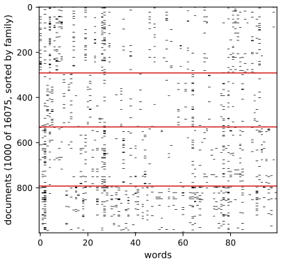
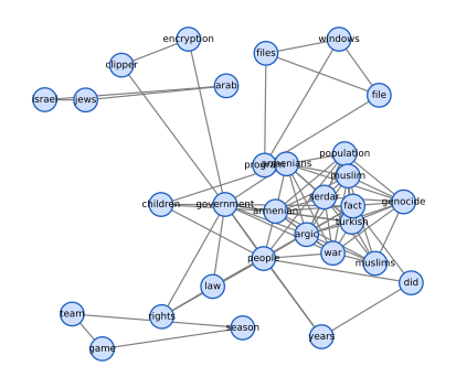
Figures and demonstrations. Every computed figure is reproduced by the Python code; Figures 5.3, 5.6, 5.7, 5.12 and 5.14 are hand-drawn sketches and information diagrams and are not reproduced. Data: Figures 5.1 and 5.5 use stand-in densities (Figure 5.5 is a two-component mixture with typical height parameters, not the published data set); Figures 5.8 and 5.9 use the public 20-newsgroups corpus grouped into the four families comp, rec, sci and talk (100 words), not the book's preprocessed matrix; Figure 5.13 uses 30 000 MNIST training digits; Figure 5.10 is a closed-form Gaussian illustration of the rate–distortion plane. The captions say so. Four original figures (5.S1 to 5.S4) illustrate results proved here. The ▶ Demo boxes open an interactive demonstration set to the case being discussed.
Main reference
K. P. Murphy, Probabilistic Machine Learning: Advanced Topics, MIT Press (2023; online draft of December 2025), Chapter 5, pages 219–259 (book page: probml.github.io/pml-book/book2.html), and the supplementary material, Chapter 5. Section, equation, figure and exercise numbers below refer to this book. The explanations, derivations, figures and code are my own. The book has no end-of-chapter exercises for this chapter; three practice problems are given instead.
Companion courses
The basics of information theory are developed in Volume 1 of this course, and those proofs are not repeated here: Chapter 6 of Probabilistic Machine Learning: An Introduction (entropy and its coding interpretation with Kraft's inequality, gap 6.1; differential entropy and quantisation, gap 6.3; non-negativity of KL, Result 6.2; KL between Gaussians, Result 6.3; the mutual information of a Gaussian pair, Result 6.4; the data processing inequality, Result 6.5; Fano's inequality, Result 6.6). Related material elsewhere on the site:
- Volume 1: 3.4 the exponential family, forward versus reverse KL for a mixture target, entropy, cross entropy and KL, binned mutual information.
- Bayesian and Probabilistic Machine Learning (Bishop): 1.6 information theory, Chapter 10 on approximate inference.
- All of Statistics: Chapter 4 on inequalities (Jensen), Chapter 9 on parametric inference (Fisher information).
What this chapter adds: the uniform-update case of the uniqueness argument for KL, the compression lemma and Donsker–Varadhan formula, the Pythagorean identity for moment projection and the supplement's reverse projection onto diagonal Gaussians, KL as a Bregman divergence in both parametrisations, typical sets and the arithmetic-coding length bound, the five variational bounds on mutual information with the InfoNCE proof, the exact slacks in the rate–distortion and variational bottleneck bounds, the self-consistent equations of the information bottleneck, and the proofs of the counting, uncomputability and total-error results of algorithmic information theory.
The chapter at a glance
- 5.1 KL from five desiderata (gap 5.1, 5.2); units, asymmetry, weight of evidence (5.3); the two projections (5.4, 5.5); compression lemma and data processing (5.6, 5.7); MLE and Bayes as KL problems (5.8, 5.9); exponential families, Fisher information, Bregman (5.10, 5.11).
- 5.2 Entropy and its units (gap 5.12); typical sets (5.13); perplexity (5.14).
- 5.3 MI identities, data processing, sufficiency (gap 5.15); multivariate information (5.16); variational bounds (5.17); relevance networks (5.18).
- 5.4–5.5 Lossless coding (gap 5.19); rate–distortion (5.20); bits back (5.21); channel-coding posterior (5.22).
- 5.6 Information bottleneck equations (gap 5.23), variational bound (5.24), conditional entropy bottleneck (5.25).
- 5.7 Kolmogorov complexity (gap 5.26) and Solomonoff's error bound (5.27).
Notation. Logarithms are natural (nats) unless a base is written; \(\log_2\) gives bits, and \(1\) nat \(=1/\ln2\approx1.443\) bits. \(\Dkl(p\|q)=\sum_xp(x)\log\frac{p(x)}{q(x)}\) with \(0\log\frac0q=0\) and \(+\infty\) when \(q=0<p\) somewhere. \(\Hent\) is entropy, \(h\) differential entropy, \(\Hce(p,q)=-\sum_xp\log q\) cross entropy, \(\MI(X;Y)\) mutual information. \(X\to Y\to Z\) means \(X\perp Z\mid Y\).
Prerequisites. Chapters 2 to 4 of the book (distributions, the exponential family, Gaussians), Jensen's inequality, and Chapter 6 of Volume 1.
5.1 KL divergence
p. 219 Machine learning is about revising beliefs, so we need a number that says how big a revision from a belief \(q\) to a belief \(p\) is. The book argues that a short list of requirements singles out one answer, the Kullback–Leibler (KL) divergence, and that entropy and mutual information are special cases of it.
See also: Volume 1, Section 6.2 (relative entropy); the entropy and KL demo.
5.1.1 Desiderata
pp. 220–221 Write \(I[p\|q]\) for the size of the update from \(q\) to \(p\) over \(N\) outcomes. The book asks for five properties: (1) continuity; (2) non-negativity; (3) permutation invariance; (4) monotonicity for uniform distributions: the update from uniform on \(N\) outcomes to uniform on \(N'\le N\) outcomes grows with \(N\) and shrinks with \(N'\); (5) a chain rule. The card example: the suit of the next card can be described in one step, or as a colour followed by a suit within the colour, and the number must be the same. Adding the steps with weights from the new belief \(p\), for any split \(\bm x=[\bm x_L,\bm x_R]\), gives
\[ I[p(\bm x)\|q(\bm x)]=I[p(\bm x_L)\|q(\bm x_L)]+\E_{p(\bm x_L)}\big[I[p(\bm x_R\given\bm x_L)\|q(\bm x_R\given\bm x_L)]\big]. \tag{5.8} \]The weights are \(p(\bm x_L)\), not \(q(\bm x_L)\); this breaks the symmetry between \(p\) and \(q\) and is the origin of the asymmetry of KL (Section 5.1.3.2).
Filling the gap 5.1: what the chain rule and monotonicity force for uniform updates pp. 220–221, (5.8), (5.17); uniqueness cited from [Hob69; Ren61]
Derivation
The book cites the general uniqueness theorem (Renyi, 1961; Hobson, 1969). Here is the complete argument for the part the monotonicity desideratum concerns: uniform \(q\) on \(N\) outcomes and uniform \(p\) on \(N'\le N\) of them. Write \(f(N,N')\) for \(I[p\|q]\) (it depends only on \((N,N')\) by permutation invariance), and use that "no update" costs nothing, \(f(N,N)=0\).
Step 1 (additivity). Let \(q=q_1\otimes q_2\) be uniform on \(N_1N_2\) pairs and \(p=p_1\otimes p_2\) uniform on \(N_1'N_2'\) pairs. Then \(p(x_2\given x_1)=p_2(x_2)\), \(q(x_2\given x_1)=q_2(x_2)\), and (5.8) gives \[ f(N_1N_2,N_1'N_2')=f(N_1,N_1')+f(N_2,N_2'). \tag{$\ast$} \]
Step 2. Put \(\varphi(N)=f(N,1)\). By \((\ast)\), \(\varphi(N_1N_2)=\varphi(N_1)+\varphi(N_2)\), so \(\varphi(1)=0\), and \(\varphi\) is increasing. Fix integers \(a,b\ge2\), \(k\ge1\) and choose \(m\) with \(a^m\le b^k<a^{m+1}\). Then \(m\varphi(a)\le k\varphi(b)\le(m+1)\varphi(a)\) and \(m\le k\frac{\ln b}{\ln a}<m+1\), so \(|\frac{\varphi(b)}{\varphi(a)}-\frac{\ln b}{\ln a}|\le\frac1k\) for all \(k\): \(\varphi(N)=c\ln N\), \(c>0\).
Step 3. If \(N=mN'\), \((\ast)\) applied to \((N',N')\) and \((m,1)\) gives \(f(mN',N')=0+c\ln m=c\ln\frac N{N'}\); with \(c=1\) this is (5.17). For non-integer ratios monotonicity in \(N\) and \(N'\) squeezes \(f\) between integer-ratio values (the limiting step is not written out).
So on uniform updates the requirements force \(I=c\ln(N/N')\). The extension to arbitrary \(p,q\) (building them from uniform ones on rational probabilities and passing to the limit) is the content of the cited theorem and is not reproved. The next gap proves the converse: KL does satisfy all five requirements. \(\square\)
5.1.2 The KL divergence uniquely satisfies the desiderata
p. 221 The Kullback–Leibler divergence (information gain, relative entropy) is \[ \Dkl(p\|q)\triangleq\sum_{k=1}^Kp_k\log\frac{p_k}{q_k}\ \ (5.9),\qquad \Dkl(p\|q)\triangleq\int\d x\,p(x)\log\frac{p(x)}{q(x)}\ \ (5.10), \] with \(0\log\frac0q=0\) and value \(+\infty\) if \(q_k=0<p_k\) for some \(k\).
5.1.2.1 Continuity, 5.1.2.2 non-negativity, 5.1.2.3 reparameterisation, 5.1.2.4 monotonicity, 5.1.2.5 chain rule
pp. 221–223 Continuity holds because \(p\log\frac pq\to0\) as \(p\to0\) (5.11). Non-negativity is Theorem 5.1.1, \(\Dkl(p\|q)\ge0\) with equality iff \(p=q\); the Jensen proof (5.12)–(5.15) is written out in Volume 1, gap 6.5. Its use: rearrange an expression into KL terms and drop them to get a bound. Reparameterisation: for an invertible \(y=f(x)\), \[ \Dkl(p(x)\|q(x))=\int\d y\,p(y)\log\frac{p(y)\,|\d y/\d x|}{q(y)\,|\d y/\d x|}=\Dkl(p(y)\|q(y)). \tag{5.16} \] Monotonicity: uniform \(p\) on \(N'\) of the \(N\) outcomes of uniform \(q\) gives \(\log\frac N{N'}\) (5.17), the number of halvings (bisection questions) separating the two. Chain rule: \[ \Dkl(p(x,y)\|q(x,y))=\Dkl(p(x)\|q(x))+\E_{p(x)}\big[\Dkl(p(y\given x)\|q(y\given x))\big], \tag{5.20} \] with the conditional divergence \(\Dkl(p(y\given x)\|q(y\given x))\triangleq\int\d x\,p(x)\int\d y\,p(y\given x)\log\frac{p(y\given x)}{q(y\given x)}\) (5.21).
Filling the gap 5.2: KL satisfies every requirement; the chain rule and the measure-theoretic form of (5.16) pp. 221–223, (5.16)–(5.21)
Proof
Chain rule (5.20). Assume \(p\ll q\) (otherwise both sides are \(+\infty\)). Where \(p(x,y)>0\), \(\log\frac{p(x,y)}{q(x,y)}=\log\frac{p(x)}{q(x)}+\log\frac{p(y\given x)}{q(y\given x)}\). Take \(\E_{p(x,y)}\): the first term gives \(\Dkl(p(x)\|q(x))\), the second the conditional KL (5.21). Each integrand has an integrable negative part (it is a KL integrand), so the split never produces \(\infty-\infty\). Iterating, \(\Dkl(p(x_{1:n})\|q(x_{1:n}))=\sum_t\E_{p(x_{<t})}\Dkl(p(x_t\given x_{<t})\|q(x_t\given x_{<t}))\), used in gap 5.27. Weighting by \(q(x_L)\) instead would not give the log density ratio of the joint, which is why the weights in (5.8) must be those of \(p\).
Reparameterisation (5.16). Let \(f\) be a measurable bijection with measurable inverse, \(P_Y=P_X\circ f^{-1}\), \(Q_Y=Q_X\circ f^{-1}\). If \(r=\d P_X/\d Q_X\), then \(\d P_Y/\d Q_Y=r\circ f^{-1}\) (for measurable \(B\): \(P_Y(B)=\int_{f^{-1}B}r\,\d Q_X=\int_Br\circ f^{-1}\,\d Q_Y\)), so \(\int\log\frac{\d P_Y}{\d Q_Y}\d P_Y=\int\log r\,\d P_X\). With densities this is the cancellation of the Jacobian in (5.16). Numerically, \(p=\N(0.3,0.8^2)\), \(q=\N(-0.2,1.3^2)\), \(y=e^x\): the divergence between the two log-normals by quadrature is 0.248821, equal to the Gaussian formula (5.78). For non-invertible \(f\) one gets only an inequality, gap 5.7.
Monotonicity, permutation invariance are the computation (5.17) and the order-independence of a sum; non-negativity and continuity were discussed above. With gap 5.1, KL meets all five desiderata, and on uniform updates any other measure meeting them is \(c\,\Dkl\). \(\square\)
5.1.3 Thinking about KL
5.1.3.1 Units
p. 224 Changing the base of the logarithm rescales KL: bits for \(\log_2\), nats for \(\ln\); \(1\text{ bit}=\ln2\approx0.693\) nats (5.22), \(1\text{ nat}\approx1.44\) bits (5.23).
5.1.3.2 Asymmetry of the KL divergence
p. 224 For Bernoulli distributions with success probabilities \(0.443\) and \(0.975\) the book computes \(0.692\) nats \(\approx1.0\) bit one way (5.24) and \(1.38\) nats \(\approx2.0\) bits the other (5.25).
5.1.3.3 KL as expected weight of evidence
pp. 224–225 For hypotheses \(P,Q\) and data \(D\), \(\log\frac{\Pr(P\given D)}{\Pr(Q\given D)}=\log\frac{p(D)}{q(D)}+\log\frac{\Pr(P)}{\Pr(Q)}\) (5.28). Good's weight of evidence is \(w[P/Q;D]=\log\frac{p(D)}{q(D)}\) (5.29); its expectation when \(P\) is true is \(\Dkl(p\|q)\ge0\).
Filling the gap 5.3: units, the asymmetry numbers, and a tail bound for misleading evidence pp. 224–225, (5.22)–(5.29)
Derivation
Units. \(\log_2y=\ln y/\ln2\), so every divergence, entropy and mutual information in bits is the value in nats divided by \(\ln2\); all identities of the chapter are homogeneous in the base.
The Bernoulli numbers. \(0.975\ln\frac{0.975}{0.443}+0.025\ln\frac{0.025}{0.557}=0.7692-0.0776=0.6916\) nats \(=0.998\) bits; the reverse is \(0.443\ln\frac{0.443}{0.975}+0.557\ln\frac{0.557}{0.025}=-0.3495+1.7289=1.3793\) nats \(=1.990\) bits. The book's values are right and the ratio is almost exactly 2.
Linear accumulation. For i.i.d. data from \(p\), \(w=\sum_t\log\frac{p(x_t)}{q(x_t)}\) is a sum of i.i.d. terms with mean \(\Dkl(p\|q)\), so \(w/n\to\Dkl(p\|q)\) almost surely: the posterior log-odds for the truth grow at rate \(\Dkl(p\|q)\) nats per observation.
Misleading evidence is exponentially rare. \(\E_p[q(D)/p(D)]=\sum_{p(D)>0}q(D)\le1\), so by Markov's inequality, for every \(t\ge0\), \[ \Pr\nolimits_p(w\le-t)=\Pr\nolimits_p\Big(\frac{q(D)}{p(D)}\ge e^{t}\Big)\le e^{-t}, \] for every sample size. Numerically, with \(p=(0.7,0.2,0.1)\), \(q=(0.4,0.4,0.2)\) the mean of \(\log\frac pq\) over \(4\times10^5\) draws is 0.1841 against \(\Dkl(p\|q)=0.1838\). \(\square\)
5.1.4 Minimizing KL
5.1.4.1 Forwards vs reverse KL
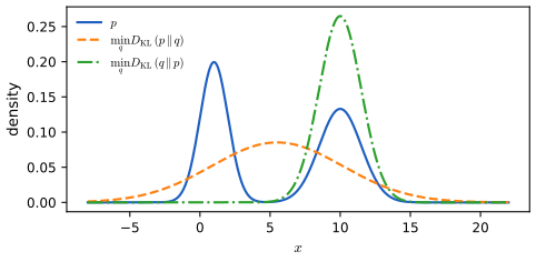
p. 225 Minimising \(\Dkl(p\|q)\) (forward, inclusive KL) forces \(q>0\) wherever \(p>0\), so \(q\) covers all modes of \(p\) (mode covering). Minimising \(\Dkl(q\|p)\) (reverse, exclusive KL) forces \(q=0\) wherever \(p=0\), so \(q\) may sit on one mode (mode seeking).
See also: Volume 1, Section 6.2.6 and its forward versus reverse KL demo.
5.1.4.2 Moment projection (mode covering)
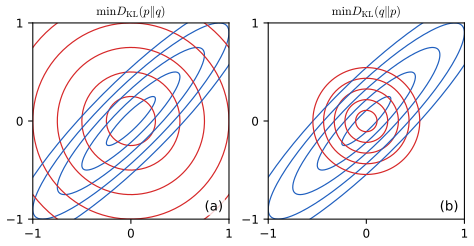
pp. 225–227 The minimiser of the forward KL, \(q=\argmin_q\Dkl(p\|q)\) (5.30), is the M-projection. For an exponential family \(q=h\exp[\bm\eta^\T\bm T-\log Z(\bm\eta)]\) (5.31) the first-order conditions (5.32)–(5.36) say \(\E_q[T_i]=\E_p[T_i]\). For correlated Gaussian \(p=\N(\bm\mu,\bm\Sigma)\) and diagonal \(q=\N(x_1\given m_1,v_1)\N(x_2\given m_2,v_2)\) (5.38): \[ q(\bm x)=\N(x_1\given\mu_1,\Sigma_{11})\,\N(x_2\given\mu_2,\Sigma_{22}), \tag{5.39} \] which covers \(p\) but is too broad (Figure 5.2a).
Filling the gap 5.4: the moment projection is the unique global minimiser and obeys a Pythagorean identity pp. 225–227, (5.30)–(5.39)
Proof
Let \(q_{\bm\eta}=h\exp[\bm\eta^\T\bm T-A(\bm\eta)]\), \(A=\log Z\), and \(p\) any distribution with \(\E_p|\bm T|<\infty\). Then \(F(\bm\eta)\triangleq\Dkl(p\|q_{\bm\eta})=-\Hent(p)-\E_p\log h-\bm\eta^\T\E_p\bm T+A(\bm\eta)\).
Convexity. Differentiating \(e^{A}=\int h\,e^{\bm\eta^\T\bm T}\) under the integral gives \(\nabla A=\E_{\bm\eta}\bm T\), \(\nabla^2A=\cov_{\bm\eta}\bm T\succeq0\) (Volume 1, Section 3.4). So \(F\) is convex with \(\nabla F=\E_{\bm\eta}\bm T-\E_p\bm T\) ((5.35)–(5.36)); every stationary point is a global minimum, unique if the family is minimal (\(\nabla^2A\succ0\)). It exists when \(\E_p\bm T\) is in the interior of the mean-parameter set.
Pythagoras. If \(\E_{q^*}\bm T=\E_p\bm T\), then for every \(\bm\eta\) \[ \Dkl(p\|q_{\bm\eta})-\Dkl(p\|q^*)=\E_p\big[(\bm\eta^*-\bm\eta)^\T\bm T-A(\bm\eta^*)+A(\bm\eta)\big]=\E_{q^*}[\cdots]=\Dkl(q^*\|q_{\bm\eta}), \] since the integrand is linear in \(\bm T\). So \(\Dkl(p\|q)=\Dkl(p\|q^*)+\Dkl(q^*\|q)\) on the family, and \(q^*\) is the unique minimiser again.
Diagonal Gaussians. Statistics \((x_i,x_i^2)\): \(m_i=\mu_i\), \(v_i=\Sigma_{ii}\) (5.39). For the bimodal \(p\) of Figure 5.1: mean \(\frac12(1+10)=5.5\), variance \(\frac12(1+1)+\frac12(2.25+100)-5.5^2=21.875\), \(\sigma=4.677\); numerical minimisation of \(\Dkl(p\|q)\) agrees to four decimals (minimum 0.647). For a Gaussian target the minimum over diagonal \(q\) is the total correlation (gap 5.16), \(-\frac12\log(1-\rho^2)\) for unit variances. With \(p\) the empirical distribution, the M-projection is the MLE (gap 5.8). \(\square\)
5.1.4.3 Information projection (mode seeking) supplement 5.1
p. 227; Supp. pp. 49–50 The minimiser of reverse KL, \(q=\argmin_q\Dkl(q\|p)\) (5.40), is the I-projection; it is easier because expectations are under the tractable \(q\) (the basis of variational inference). For \(p=\N(\bm\mu,\bm\Lambda^{-1})\) and diagonal \(q\) the optimum is \(\bm m=\bm\mu\), \(v_i=\Lambda_{ii}^{-1}\) (Supp. 5.1.2): the variances match the marginal precisions, so \(q\) is overconfident (Figure 5.2b). Reverse KL is not always too narrow [Tur+08].
Filling the gap 5.5 supplement: the reverse KL projection onto diagonal Gaussians p. 227; Supp. (5.1)–(5.9)
Derivation
Moment projection (Supp. 5.1.1). Done in gap 5.4.
Information projection (Supp. 5.1.2). By (5.77), with \(\bm\Lambda=\bm\Sigma^{-1}\), \(\bm V=\diag(\bm v)\), \[ \Dkl(\N(\bm m,\bm V)\|\N(\bm\mu,\bm\Sigma))=\tfrac12\Big[\log\frac{|\bm\Sigma|}{|\bm V|}-D+(\bm\mu-\bm m)^\T\bm\Lambda(\bm\mu-\bm m)+\Tr(\bm\Lambda\bm V)\Big]. \] (The supplement's (5.5) prints \(\bm\Sigma\) in the quadratic term where \(\bm\Lambda\) belongs; since \(\bm\Lambda\succ0\), the conclusion \(\bm m=\bm\mu\) is unchanged.) With \(\bm m=\bm\mu\) and diagonal \(\bm V\), \(J(\bm v)=\frac12\sum_i(\Lambda_{ii}v_i-\log v_i)+\mathrm{const}\), separable and convex in each \(v_i\) with derivative \(\frac12(\Lambda_{ii}-1/v_i)\): \(v_i=1/\Lambda_{ii}\) (Supp. (5.8)–(5.9)), the conditional variance of \(x_i\) given the rest.
Narrower. Cauchy–Schwarz: \(1=(\bm e_i^\T\bm e_i)^2=(\bm e_i^\T\bm\Lambda^{1/2}\bm\Sigma^{1/2}\bm e_i)^2\le\Lambda_{ii}\Sigma_{ii}\), so \(1/\Lambda_{ii}\le\Sigma_{ii}\), with equality iff \(\bm e_i\) is an eigenvector of \(\bm\Sigma\). For two unit-variance coordinates \(\Lambda_{ii}=1/(1-\rho^2)\): the reverse variance is \(1-\rho^2\) times the forward one (0.19 at \(\rho=0.9\), 0.0199 at \(\rho=0.99\)).
Minimum values. The reverse minimum is \(\frac12\log(|\bm\Sigma|\prod_i\Lambda_{ii})\), which for two unit-variance coordinates is \(-\frac12\log(1-\rho^2)=\MI(x_1;x_2)\), the same as the forward minimum. The cross values also coincide in two dimensions: \(\Dkl(q_{\rm fwd}\|p)=\Dkl(p\|q_{\rm rev})=\frac12[\frac2{1-\rho^2}-2+\log(1-\rho^2)]=3.4328\) at \(\rho=0.9\) (it uses \(|\bm\Lambda|=1/|\bm\Sigma|\) and \(\Sigma_{ii}=\Lambda_{jj}/|\bm\Lambda|\), so needs \(D=2\)). A generic optimiser over the variances reproduces \(1/\Lambda_{ii}\) to five decimals. \(\square\)
5.1.5 Properties of KL
5.1.5.1 Compression lemma
p. 228 For any \(P,Q\) with well-defined divergence and any scalar function \(\phi\), \[ \E_P[\phi]\le\log\E_Q\big[e^{\phi}\big]+\Dkl(P\|Q), \tag{5.41} \] proved in the book from \(\Dkl(P\|G)\ge0\) for \(g=qe^\phi/Z\) (5.42)–(5.44). Equivalently the Donsker–Varadhan representation \[ \Dkl(P\|Q)=\sup_\phi\ \E_P[\phi]-\log\E_Q[e^{\phi}], \tag{5.45} \] the engine of PAC-Bayes bounds (Section 17.4.5) and of the bounds of Section 5.3.6.
Filling the gap 5.6: the supremum in (5.45) is attained or approached, and when equality holds p. 228, (5.41)–(5.45)
Proof
(5.41). Assume \(Z=\E_Qe^\phi\in(0,\infty)\) and finite \(\Dkl(P\|Q)\). Then \(0\le\Dkl(P\|G)=\E_P[\log\frac pq-\phi+\log Z]=\Dkl(P\|Q)-\E_P\phi+\log Z\). Equality iff \(P=G\), i.e. \(\phi=\log\frac pq+c\) \(P\)-a.s.
(5.45). By (5.41) the sup is \(\le\Dkl(P\|Q)\). Take \(\phi_n=\min(\log\frac pq,n)\): \(\E_P\phi_n\to\Dkl(P\|Q)\) by monotone convergence, and \(\E_Qe^{\phi_n}=\E_Q\min(p/q,e^n)\le1\), so \(\log\E_Qe^{\phi_n}\le0\); hence \(\E_P\phi_n-\log\E_Qe^{\phi_n}\ge\E_P\phi_n\to\Dkl(P\|Q)\). The sup is attained when \(\log\frac pq\) is bounded, otherwise approached; if the KL is infinite so is the sup.
Use. Any \(\phi\) (e.g. a neural critic) gives a lower bound exact when \(\phi\) is the log density ratio up to a constant; it needs only samples from \(P\) and \(Q\). A random-\(\phi\) check on a 7-point space confirms (5.41) and equality at \(\phi=\log\frac pq+1.234\). \(\square\)
5.1.5.2 Data processing inequality for KL
pp. 229–230 Sending samples of \(p(x)\) and \(q(x)\) through the same channel \(t(y\given x)\) gives \(p(y),q(y)\) with \[ \Dkl(p(x)\|q(x))\ge\Dkl(p(y)\|q(y)) \tag{5.46} \] (Theorem 5.1.3). Marginalising is a special channel: \(\Dkl(p(x,y)\|q(x,y))\ge\Dkl(p(x)\|q(x))\) (5.54).
Filling the gap 5.7: a two-line proof of (5.46) and (5.54) by the chain rule, with the equality case pp. 229–230, (5.46)–(5.59)
Proof
With \(p(x,y)=p(x)t(y\given x)\), \(q(x,y)=q(x)t(y\given x)\), expand \(\Dkl(p(x,y)\|q(x,y))\) in two orders. Conditioning on \(x\): \(=\Dkl(p(x)\|q(x))+\E_{p(x)}\Dkl(t\|t)=\Dkl(p(x)\|q(x))\). Conditioning on \(y\): \(=\Dkl(p(y)\|q(y))+\E_{p(y)}\Dkl(p(x\given y)\|q(x\given y))\ge\Dkl(p(y)\|q(y))\). Equating gives (5.46) and shows the loss is exactly \(\E_{p(y)}\Dkl(p(x\given y)\|q(x\given y))\); equality iff \(p(x\given y)=q(x\given y)\) a.e., i.e. \(y\) is sufficient for telling \(p\) from \(q\). Marginalisation (5.54) is the channel returning one coordinate.
Mutual information. For \(X\to Y\to Z\) take \(p(x,y)\), \(q=p(x)p(y)\) and the channel \((x,y)\mapsto(x,z)\); the outputs are \(p(x,z)\), \(p(x)p(z)\), and (5.46) reads \(\MI(X;Y)\ge\MI(X;Z)\) (see also Volume 1, Result 6.5). A random 5-state channel check confirms (5.46) and (5.54). \(\square\)
5.1.6 KL divergence and MLE
pp. 230–231 With \(p_{\mathcal D}(x)=\frac1N\sum_n\delta(x-x_n)\) (5.61), \(\Dkl(p_{\mathcal D}\|q)=-\frac1N\sum_n\log q(x_n)+C\) (5.64), i.e. \(\Hce(p_{\mathcal D},q)-\Hent(p_{\mathcal D})\) (5.65) with \(\Hce(p,q)=-\sum_kp_k\log q_k\) (5.66): minimising KL to the data distribution is maximum likelihood. The flaw: \(p_{\mathcal D}\) is a set of spikes, so the fit overfits and needs smoothing or regularisation.
Filling the gap 5.8: what (5.62)–(5.65) means for continuous data, and what the MLE aims at pp. 230–231, (5.60)–(5.66)
Derivation
Discrete case. \(p_{\mathcal D}\) is a genuine distribution and (5.65) is an identity; only \(\Hce(p_{\mathcal D},q)=-\frac1N\sum\log q(x_n)\) depends on \(q\), so \(\argmin_q\Dkl(p_{\mathcal D}\|q)=\argmax_q\prod_nq(x_n)\). (For 50 simulated Bernoulli draws, the grid minimisers of the NLL and of \(\Dkl(p_{\mathcal D}\|q_\theta)\) coincide with the sample frequency.)
Continuous case. \(p_{\mathcal D}\) is not absolutely continuous w.r.t. \(q\), so strictly \(\Dkl(p_{\mathcal D}\|q)=+\infty\) and \(C=-\infty\) in (5.62). The equations must be read for the finite cross entropy (5.65); the conclusion (MLE \(=\) cross-entropy minimiser) is unaffected.
What the MLE converges to. For \(x_n\sim p^*\) i.i.d., \(\Hce(p_{\mathcal D},q_\theta)\to\Hent(p^*)+\Dkl(p^*\|q_\theta)\) a.s. for each \(\theta\); under uniformity conditions the MLE converges to the pseudo-true parameter \(\theta^*=\argmin_\theta\Dkl(p^*\|q_\theta)\) (White, 1982), the M-projection of the truth, and to the truth if the model contains it and is identifiable. In an exponential family the empirical M-projection is the MLE (gap 5.4). \(\square\)
5.1.7 KL divergence and Bayesian inference
pp. 231–232 From a joint prior \(q(\bm\theta,\mathcal D)=q(\bm\theta)q(\mathcal D\given\bm\theta)\), after seeing \(\mathcal D_0\) choose the closest joint consistent with the data, \[ p(\bm\theta,\mathcal D)=\argmin\Dkl(p(\bm\theta,\mathcal D)\|q(\bm\theta,\mathcal D))\quad\text{s.t.}\quad p(\mathcal D)=\delta(\mathcal D-\mathcal D_0). \tag{5.67} \] The chain rule (5.68) gives \(p=\delta(\mathcal D-\mathcal D_0)q(\bm\theta\given\mathcal D)\) (5.69), with \(\bm\theta\)-marginal the posterior (5.70). If the data are known only up to \(p(\mathcal D)\), \(p(\bm\theta)=\int\d\mathcal D\,p(\mathcal D)q(\bm\theta\given\mathcal D)\) (5.72): Jeffrey's conditionalisation.
Filling the gap 5.9: Bayes' rule and Jeffrey's rule as KL projections pp. 231–232, (5.67)–(5.72)
Proof
Let \(\mathcal D\) be discrete, \(q(\mathcal D_0)>0\). Any \(p\) with \(p(\mathcal D)=r(\mathcal D)\) is \(r(\mathcal D)p(\bm\theta\given\mathcal D)\), and by the chain rule \[ \Dkl(p\|q)=\Dkl(r\|q(\mathcal D))+\sum_{\mathcal D}r(\mathcal D)\Dkl\big(p(\bm\theta\given\mathcal D)\|q(\bm\theta\given\mathcal D)\big). \tag{5.68} \] The first term is fixed by the constraint; the second is \(\ge0\), zero iff \(p(\bm\theta\given\mathcal D)=q(\bm\theta\given\mathcal D)\) wherever \(r>0\). So the unique minimiser keeps the prior conditionals, with minimum \(\Dkl(r\|q(\mathcal D))\). With \(r=\delta_{\mathcal D_0}\) the minimum is \(-\log q(\mathcal D_0)\) and \(p(\bm\theta)=q(\bm\theta)q(\mathcal D_0\given\bm\theta)/q(\mathcal D_0)\); with general \(r\), \(p(\bm\theta)=\sum r(\mathcal D)q(\bm\theta\given\mathcal D)\) (5.72). A check with a 3-point \(\bm\theta\), 4-valued \(\mathcal D\) and random prior returns the exact posterior to five decimals.
Remarks. (i) For continuous \(\mathcal D\) the first term of (5.68) is infinite for every feasible \(p\) but identical across them (make it rigorous with a narrow density instead of the delta). (ii) Bayes' rule as the product rule does not say one should adopt the conditional; the minimum-KL principle does. (iii) If the posterior is restricted to a family, the best member minimises \(\Dkl(p(\bm\theta\given\mathcal D_0)\|q(\bm\theta\given\mathcal D_0))\): variational inference (Bishop's Chapter 10). \(\square\)
5.1.8 KL divergence and exponential families
pp. 232–233 For \(p(x\given\bm\eta)=h\exp[\bm\eta^\T\bm T-A(\bm\eta)]\) (5.73, 5.74), \[ \Dkl(p(x\given\bm\eta_1)\|p(x\given\bm\eta_2))=(\bm\eta_1-\bm\eta_2)^\T\bm\mu_1-A(\bm\eta_1)+A(\bm\eta_2),\qquad\bm\mu_1=\E_{\bm\eta_1}\bm T, \tag{5.75, 5.76} \] and for Gaussians (Example 5.1.8.1) \[ \Dkl(\N(\bm\mu_1,\bm\Sigma_1)\|\N(\bm\mu_2,\bm\Sigma_2))=\tfrac12\Big[\Tr(\bm\Sigma_2^{-1}\bm\Sigma_1)+(\bm\mu_2-\bm\mu_1)^\T\bm\Sigma_2^{-1}(\bm\mu_2-\bm\mu_1)-D+\log\frac{|\bm\Sigma_2|}{|\bm\Sigma_1|}\Big], \tag{5.77} \] which is \(\log\frac{\sigma_2}{\sigma_1}+\frac{\sigma_1^2+(\mu_1-\mu_2)^2}{2\sigma_2^2}-\frac12\) in one dimension (5.78); derived in Volume 1, Result 6.3.
5.1.9 Approximating KL using the Fisher information matrix
p. 233 For \(\bm\theta'=\bm\theta+\bm\delta\), a second-order expansion (5.79)–(5.80) and the zero expected score give \[ \Dkl(p_{\bm\theta}\|p_{\bm\theta'})\approx\tfrac12\bm\delta^\T\bm F(\bm\theta)\bm\delta,\qquad\bm F=-\E[\nabla^2\log p_{\bm\theta}]=\E[\nabla\log p_{\bm\theta}\nabla\log p_{\bm\theta}^\T], \tag{5.81, 5.82} \] a squared Mahalanobis distance in the Fisher metric, the basis of natural gradients (Section 6.4).
5.1.10 Bregman divergence
pp. 233–234 For differentiable strictly convex \(f\), \(B_f(\bm w\|\bm v)=f(\bm w)-f(\bm v)-(\bm w-\bm v)^\T\nabla f(\bm v)\ge0\) (5.83)–(5.85; Figure 5.3a is a sketch): squared Euclidean distance for \(f=\|\bm w\|^2\), squared Mahalanobis distance for \(f=\bm w^\T\bm Q\bm w\). 5.1.10.1: with \(f=A\), \(B_A(\bm\eta_q\|\bm\eta_p)=A(\bm\eta_q)-A(\bm\eta_p)-(\bm\eta_q-\bm\eta_p)^\T\E_p\bm T=\Dkl(p\|q)\) (5.86)–(5.88). KL is the only divergence that is both Bregman and an \(f\)-divergence [Ama09] (cited, not proved).
Filling the gap 5.10: exponential-family KL and its Bregman form in both parametrisations pp. 232–234, (5.73)–(5.88)
Proof
(5.75)–(5.76). The base measure cancels: \(\log\frac{p(x|\bm\eta_1)}{p(x|\bm\eta_2)}=(\bm\eta_1-\bm\eta_2)^\T\bm T-A(\bm\eta_1)+A(\bm\eta_2)\); take \(\E_{\bm\eta_1}\) with \(\E_{\bm\eta_1}\bm T=\nabla A(\bm\eta_1)\) (gap 5.4).
(5.86)–(5.88). \(A\) is convex (\(\nabla^2A=\cov\bm T\succeq0\)) and \(B_A(\bm\eta_2\|\bm\eta_1)=A(\bm\eta_2)-A(\bm\eta_1)-(\bm\eta_2-\bm\eta_1)^\T\bm\mu_1\) equals (5.76). So \(\Dkl(p_1\|p_2)=B_A(\bm\eta_2\|\bm\eta_1)\), with the natural parameters in reversed order (the book's \(B_f(\bm\eta_q\|\bm\eta_p)=\Dkl(p\|q)\)). Non-negativity is the supporting-hyperplane inequality, strict for minimal families.
Mean parameters. With \(A^*(\bm\mu)=\sup_{\bm\eta}\bm\eta^\T\bm\mu-A\), at \(\bm\mu=\nabla A(\bm\eta)\): \(A^*=\bm\eta^\T\bm\mu-A(\bm\eta)\), \(\nabla A^*=\bm\eta\). Then \(B_{A^*}(\bm\mu_1\|\bm\mu_2)=A^*(\bm\mu_1)-A^*(\bm\mu_2)-(\bm\mu_1-\bm\mu_2)^\T\bm\eta_2=(\bm\eta_1-\bm\eta_2)^\T\bm\mu_1-A(\bm\eta_1)+A(\bm\eta_2)=\Dkl(p_1\|p_2)\): the same KL is a Bregman divergence of \(A^*\) with arguments in natural order.
Examples. Poisson (\(A=e^\eta\)): \(\Dkl=\lambda_1\log\frac{\lambda_1}{\lambda_2}-\lambda_1+\lambda_2\), 0.403952 at \(\lambda=(3,1.7)\), equal to direct summation and to \(B_A\). Gaussian with known variance: \(A=\eta^2\sigma^2/2\), \(B_A=\frac{(\mu_1-\mu_2)^2}{2\sigma^2}\). For \(f=\bm w^\T\bm Q\bm w\), \(B_f=(\bm w-\bm v)^\T\bm Q(\bm w-\bm v)\). A Monte Carlo estimate of (5.77) for two 2-D Gaussians (\(4\times10^5\) draws) gives 0.4821 against 0.4819. \(\square\)
Filling the gap 5.11: the Fisher approximation (5.81) and its error order p. 233, (5.79)–(5.82)
Derivation
Assume a regular model (three times differentiable in \(\bm\theta\), fixed support, differentiation under the integral). Score. \(0=\int\nabla p_{\bm\theta}=\E[\nabla\log p_{\bm\theta}]\). Information equality. Differentiating \(\int p_{\bm\theta}\nabla\log p_{\bm\theta}=0\) gives \(\E\nabla^2\log p_{\bm\theta}+\E[\nabla\log p_{\bm\theta}\nabla\log p_{\bm\theta}^\T]=0\), so the two forms of \(\bm F\) in (5.82) agree.
Expansion. \(\log p_{\bm\theta+\bm\delta}=\log p_{\bm\theta}+\bm\delta^\T\bm s+\frac12\bm\delta^\T\bm H\bm\delta+R_3\), \(|R_3|\le C(x)\|\bm\delta\|^3\). Then \(\Dkl(p_{\bm\theta}\|p_{\bm\theta+\bm\delta})=-\bm\delta^\T\E\bm s-\frac12\bm\delta^\T\E\bm H\bm\delta-\E R_3=\frac12\bm\delta^\T\bm F\bm\delta+O(\|\bm\delta\|^3)\) if \(\E C<\infty\). Only local: far away KL can be infinite while the quadratic is finite.
Exponential families. It is the Taylor expansion of \(A\) in \(B_A\): \(\nabla^2A=\cov\bm T=\bm F(\bm\eta)\). Both directions agree to second order. Numerics. For the Bernoulli, \(F=1/(\theta(1-\theta))\); at \(\theta=0.3\) the error is \(1.70\times10^{-4},2.27\times10^{-5},2.93\times10^{-6}\) for \(\delta=0.04,0.02,0.01\): a factor 7 to 8 per halving, an \(O(\delta^3)\) error. For \(\N(\mu,\sigma^2)\) in \((\mu,\sigma)\), \(\bm F=\diag(1/\sigma^2,2/\sigma^2)\). \(\square\)
5.2 Entropy
See also: Volume 1, Section 6.1; the entropy, cross entropy and KL demo.
5.2.1 Definition
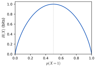
p. 235 \(\Hent(X)=-\sum_kp(X=k)\log p(X=k)\) (5.89), a constant minus the divergence from the uniform \(u\): \[ \Hent(X)=\log K-\Dkl(p\|u), \tag{5.90}\text{--}(5.92) \] so it is maximal (\(\log K\)) for the uniform. For a binary variable, \(\Hent(\theta)=-[\theta\log\theta+(1-\theta)\log(1-\theta)]\) (5.93, 5.94), maximal at 1 bit for \(\theta=\frac12\) (Figure 5.4).
5.2.2 Differential entropy for continuous random variables
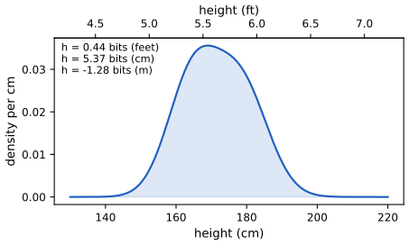
pp. 235–236 \(h(X)=-\int\d x\,p(x)\log p(x)\) (5.95); for a Gaussian \(h=\frac12\log|2\pi e\bm\Sigma|\) (5.96), \(\frac12\log(2\pi e\sigma^2)\) in 1-D (5.97). It can be negative: \(X\sim U(0,a)\) has \(h=\log a\) (5.98), \(-3\) bits at \(a=\frac18\). An \(n\)-bit quantisation has entropy about \(h(X)+n\). Unlike KL it is not invariant to changes of variable: \[ h(X)=h(Y)-\int\d y\,p(y)\log\Big|\frac{\d y}{\d x}\Big|, \tag{5.99, 5.100} \] so it depends on units (Figure 5.5).
Filling the gap 5.12: entropy as KL from uniform, differential entropy as KL from Lebesgue measure, and the numbers of Figure 5.5 pp. 235–236, (5.90)–(5.100)
Derivation
(5.90). \(\Dkl(p\|u)=\sum p_k\log(Kp_k)=\log K-\Hent(p)\), so \(\Hent\le\log K\) with equality iff \(p=u\). Gaussian, uniform and quantisation statements are proved in Volume 1, gap 6.3.
Units. Formally \(h(X)=-\Dkl(p\|\lambda)\) with Lebesgue measure \(\lambda\), which is not a probability measure. KL is invariant when both measures are transformed (gap 5.2), but \(\lambda\) transforms into \(|\d x/\d y|\d y\), a different reference: that is the Jacobian term in (5.100). For \(y=cx\), \(h(cX)=h(X)+\log|c|\); for \(\bm y=\bm A\bm x\), \(h=h+\log|\det\bm A|\).
Numbers. By quadrature \(h=5.365\) bits in centimetres; scaling lengths by \(1/30.48\) shifts it by \(-4.930\) (0.436 bits in feet) and by \(1/100\) by \(-6.644\) (\(-1.278\) bits in metres). \(U(0,\frac18)\): \(\log_2\frac18=-3\). \(\square\)
5.2.3 Typical sets
pp. 236–237 The \(\epsilon\)-typical set \(A_\epsilon^N\subseteq\mathcal X^N\) is the set of sequences with \[ \Hent(p)-\epsilon\le-\frac1N\log p(x_1,\dots,x_N)\le\Hent(p)+\epsilon. \tag{5.101} \] For i.i.d. data the middle term converges in probability to \(\Hent(p)\) (the asymptotic equipartition property, AEP), so the typical set has probability near 1.
Filling the gap 5.13: the AEP, the size of the typical set, and its use for compression pp. 236–237, (5.101); [CT06]
Proof
Let \(Z_n=-\log p(X_n)\) i.i.d. on a finite alphabet: mean \(\Hent\), variance \(\sigma^2<\infty\).
Probability. Chebyshev: \(\Pr(X^N\notin A_\epsilon^N)\le\sigma^2/(N\epsilon^2)\to0\).
Size. On \(A_\epsilon^N\), \(p(x^N)\ge e^{-N(\Hent+\epsilon)}\), so \(1\ge|A_\epsilon^N|e^{-N(\Hent+\epsilon)}\): \(|A_\epsilon^N|\le e^{N(\Hent+\epsilon)}\). Also \(p\le e^{-N(\Hent-\epsilon)}\) there, so for \(N\) large with \(\Pr(A)\ge1-\delta\), \(|A_\epsilon^N|\ge(1-\delta)e^{N(\Hent-\epsilon)}\).
Compression. Send a flag bit, then the index among typical sequences (\(\lceil N(\Hent+\epsilon)\rceil\) bits) or, for atypical ones, among all \(|\mathcal X|^N\). Expected length per symbol \(\le\Hent+\epsilon+\delta\log|\mathcal X|+2/N\). The converse (nothing below \(\Hent\)) is Kraft's inequality, Volume 1, gap 6.1.
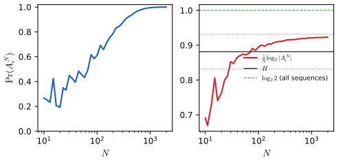
Cautions. The typical set is not the set of most probable sequences: for Bernoulli(0.3) the all-zeros sequence is the most probable, with \(-\frac1N\log_2p=0.515\) bits against \(\Hent=0.881\), so it is atypical for \(\epsilon=0.05\). Exact binomial sums give \(\Pr(A_{0.05}^N)=0.449,0.674,0.928,0.9999989\) at \(N=30,100,400,3000\) (Figure 5.S1); at \(N=400\), \(\frac1N\log_2|A|=0.916\in[0.831,0.931]\). \(\square\)
5.2.4 Cross entropy and perplexity
pp. 237–238 \(\Dkl(p\|q)=\Hce(p,q)-\Hent(p)\) (5.102, 5.103). Language models report the perplexity \(2^{\Hce(p,q)}\) (5.104); for data it is \((\prod_np(x_n))^{-1/N}\) (5.105–5.108). A uniform model \(p(x_n\given x_{n-1})=1/K\) has perplexity \(K\), the branching factor. The book states perplexity can never go below \(2^{-\Hent(p^*)}\).
Filling the gap 5.14: perplexity and its lower bound (the sign in the book's last sentence) pp. 237–238, (5.102)–(5.108)
Derivation
Bound. \(\Hce(p^*,q)=\Hent(p^*)+\Dkl(p^*\|q)\ge\Hent(p^*)\), so \(2^{\Hce}=2^{\Hent(p^*)}\cdot2^{\Dkl(p^*\|q)}\ge2^{+\Hent(p^*)}\). The book prints \(2^{-\Hent(p^*)}\le1\), which is no bound of interest (Notes on the book). The factor \(2^{\Dkl}\) is the multiplicative price of a wrong model.
Base independence. \(b^{\Hce^{(b)}}=e^{\Hce^{(e)}}\), so the perplexity is \(\exp(\text{mean NLL in nats})\).
Conditional models. By the chain rule of probability the likelihood is \(\prod_nq(x_n\given x_{<n})\) and the perplexity \(\exp(-\frac1N\sum\log q(x_n\given x_{<n}))\). A model of perplexity \(B\) has the code length of a uniform choice among \(B\) symbols.
Numerics. For a 5-symbol source, the simulated perplexity of the true model matches \(2^{\Hent}\) within 0.02, wrong models are larger, and the uniform model has perplexity exactly 5. \(\square\)
5.3 Mutual information
See also: Volume 1, Section 6.3; the binned mutual information demo.
5.3.1 Definition
pp. 238–239 \(\MI(X;Y)\triangleq\Dkl(p(x,y)\|p(x)p(y))\) (5.109), \(\ge0\) with equality iff independent (5.110).
5.3.2 Interpretation
p. 239 \(\MI(X;Y)=\Hent(X)-\Hent(X|Y)=\Hent(Y)-\Hent(Y|X)\) (5.111); \(=\Hent(X,Y)-\Hent(X|Y)-\Hent(Y|X)\) (5.112); \(=\Hent(X)+\Hent(Y)-\Hent(X,Y)\) (5.113). Conditioning reduces entropy on average. Figure 5.6 is an information diagram (a sketch).
5.3.3 Data processing inequality
p. 239 If \(X\to Y\to Z\) then \(\MI(X;Y)\ge\MI(X;Z)\) (Theorem 5.3.1), proved by expanding \(\MI(X;Y,Z)\) two ways (5.114)–(5.116).
5.3.4 Sufficient statistics
pp. 240–241 For \(\theta\to X\to s(X)\), \(\MI(\theta;s(X))\le\MI(\theta;X)\) (5.117); \(s\) is sufficient if equality holds (and then \(\theta\to s(X)\to X\)), minimal if it is a function of every sufficient statistic (5.118). For Bernoulli trials \((N,N_1)\) is minimal. The Pitman–Koopman–Darmois theorem: for fixed support only exponential families have bounded-dimensional sufficient statistics [Dia88b].
Filling the gap 5.15: the MI identities, chain rule, data processing with equality case, and sufficiency as factorisation pp. 238–241, (5.110)–(5.118)
Proof
(5.111)–(5.113). \(\MI=\sum p(x,y)\log\frac{p(x|y)}{p(x)}=\Hent(X)-\Hent(X|Y)\), and symmetrically. With \(\Hent(X,Y)=\Hent(Y)+\Hent(X|Y)\) the other two forms are algebra. Hence \(\Hent(X|Y)\le\Hent(X)\) on average (not for each \(y\)).
Chain rule. With \(\MI(X;Y|Z)=\Hent(X|Z)-\Hent(X|Y,Z)\ge0\), \(\MI(X;Y,Z)=[\Hent(X)-\Hent(X|Z)]+[\Hent(X|Z)-\Hent(X|Y,Z)]=\MI(X;Z)+\MI(X;Y|Z)\) (5.114), and symmetrically (5.115).
Data processing. \(X\perp Z\mid Y\) gives \(\MI(X;Z|Y)=0\), so \(\MI(X;Y,Z)=\MI(X;Y)\) and \(\MI(X;Y)=\MI(X;Z)+\MI(X;Y|Z)\ge\MI(X;Z)\). Equality iff \(\MI(X;Y|Z)=0\): \(Z\) keeps everything \(Y\) knows about \(X\). It also follows from gap 5.7.
Sufficiency. Since \(s\) is a function of \(X\), \(\MI(\theta;X)=\MI(\theta;s(X))+\MI(\theta;X|s(X))\). Equality iff \(\MI(\theta;X|s)=0\) iff \(p(x|\theta,s(x)=t)\) is free of \(\theta\) iff \(p(x|\theta)=g(s(x),\theta)r(x)\) (Fisher–Neyman). Bernoulli: \(\theta^{N_1}(1-\theta)^{N-N_1}\) depends on \(x\) only through \(N_1\). Numerically, for four flips and a three-point prior, \(\MI(\theta;\text{sum})=\MI(\theta;\text{sequence})\) while the first flip alone gives strictly less.
PKD. Easy half: for \(h(x)\exp[\bm\eta(\theta)^\T\bm T-A(\theta)]\), \(\sum_n\bm T(x_n)\) is sufficient of fixed dimension (Gaussian: \(\sum x_n,\sum x_n^2\); two data sets with equal sums have a parameter-free likelihood ratio, checked). The converse needs smoothness and a differentiation argument and is cited, not proved. \(\square\)
5.3.5 Multivariate mutual information
5.3.5.1 Total correlation
p. 241 \(\mathrm{TC}=\Dkl(p(\bm x)\|\prod_dp(x_d))=\sum_d\Hent(x_d)-\Hent(\bm x)\) (5.119–5.121): \(\ge0\), zero iff independent, but positive when only one pair interacts.
5.3.5.2 Interaction information, 5.3.5.3 synergy and redundancy, 5.3.5.4 MMI and causality, 5.3.5.5 MMI and entropy
pp. 241–244 \(\MI(X_1;\cdots;X_D)=\MI(X_1;\cdots;X_{D-1})-\MI(X_1;\cdots;X_{D-1}|X_D)\) (5.123); for three variables \(\MI(X;Y;Z)=\MI(X;Y)-\MI(X;Y|Z)\) (5.124)–(5.126), symmetric, \(=\MI(X;Z)+\MI(Y;Z)-\MI(X,Y;Z)\) (5.128). Positive means redundancy, negative synergy. It is \(\ge0\) for a common cause and a Markov chain, \(\le0\) for a collider (e.g. XOR). In entropies \[ \MI(X;Y;Z)=[\Hent(X)+\Hent(Y)+\Hent(Z)]-[\Hent(X,Y)+\Hent(X,Z)+\Hent(Y,Z)]+\Hent(X,Y,Z), \tag{5.131} \] generally \(\MI(X_1,\dots,X_D)=-\sum_{T}(-1)^{|T|}\Hent(T)\) (5.132) with dual \(\Hent(S)=-\sum_{T\subseteq S}(-1)^{|T|}\MI(T)\) (5.136) (Mobius inversion), and \(\MI(X;Y;Z)=\Hent(Z)-\Hent(Z|X)-\Hent(Z|Y)+\Hent(Z|X,Y)\) (5.137). Figure 5.7 is a sketch.
Filling the gap 5.16: total correlation, symmetry and signs of the three-way information, XOR, Mobius inversion pp. 241–244, (5.119)–(5.137)
Proof
TC. A KL divergence, so \(\ge0\), zero iff independent. By the chain rule \(\mathrm{TC}=\sum_d\MI(x_d;x_{<d})\). For \(p(X,Y)p(Z)\): \(\mathrm{TC}=\MI(X;Y)+\MI(Z;X,Y)=\MI(X;Y)\), so TC is not a three-way measure.
(5.131). \(\MI(X;Y)=\Hent(X)+\Hent(Y)-\Hent(X,Y)\) and \(\MI(X;Y|Z)=\Hent(X,Z)+\Hent(Y,Z)-\Hent(Z)-\Hent(X,Y,Z)\) (5.130); subtracting gives (5.131), manifestly symmetric, so (5.124)–(5.126) agree. From \(\MI(X;Y|Z)=\MI(X;Y,Z)-\MI(X;Z)\) comes (5.128). Writing out the conditional entropies gives (5.137).
Signs. Common cause: \(\MI(X;Y|Z)=0\), so \(\MI(X;Y;Z)=\MI(X;Y)\ge0\). Chain: by (5.125) \(=\MI(X;Z)-\MI(X;Z|Y)=\MI(X;Z)\ge0\). Collider: the parents are marginally independent, \(\MI(X;Y)=0\), so \(\MI(X;Y;Z)=-\MI(X;Y|Z)\le0\) (the rigorous form of explaining away, for marginally independent parents). XOR (\(Z=X\oplus Y\), fair independent bits): all pairwise \(\MI=0\), \(\MI(X;Y|Z)=1\) bit, so \(\MI(X;Y;Z)=-1\) bit, \(\mathrm{TC}=3-2=1\) bit; \(\MI(X,Y;Z)=1\) while \(\MI(X;Z)+\MI(Y;Z)=0\): pure synergy.
Mobius. Let \(f(T)=(-1)^{|T|}\Hent(T)\), \(g(S)=\sum_{T\subseteq S}f(T)=-\MI(S)\). Inversion on the Boolean lattice: \(f(S)=\sum_{T\subseteq S}(-1)^{|S|-|T|}g(T)\), since \(\sum_{T\subseteq S}(-1)^{|S|-|T|}\sum_{U\subseteq T}f(U)=\sum_Uf(U)\sum_{U\subseteq T\subseteq S}(-1)^{|S|-|T|}\) and the inner sum is \((1-1)^{|S|-|U|}\), nonzero only for \(U=S\). Substituting \(g=-\MI\) gives (5.136). Checked on a random \(3\times3\times3\) table. \(\square\)
5.3.6 Variational bounds on mutual information
pp. 244–246 When the joint or marginals are intractable (representation learning, Chapter 32), approximate them [BA03; Poo+19b].
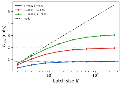
Upper bound (5.138)–(5.141). With \(q(y)\approx p(y)\): \(\MI(x;y)\le\E_{p(x)}\Dkl(p(y|x)\|q(y))\), tight at \(q=p(y)\). BA bound (5.142)–(5.144). With \(q(x|y)\approx p(x|y)\): \(\MI\ge\E_{p(x,y)}\log q(x|y)+h(x)\). DV and NWJ (5.145)–(5.150). With \(q(x|y)=p(x)e^{f}/Z(y)\), \(Z(y)=\E_{p(x)}e^{f}\): \(\MI_{\rm DV}=\E_{p(x,y)}f-\E_{p(y)}\log Z(y)\) (5.148); and with \(\log x\le x/a+\log a-1\) at \(a=e\), \(\MI\ge\E_{p(x,y)}f-e^{-1}\E_{p(y)}Z(y)\) (5.150) (NWJ). InfoNCE (5.151, 5.152). For a batch of \(K\) pairs, \[ \MI_{\rm NCE}=\E\Big[\frac1K\sum_{i}\log\frac{e^{f(x_i,y_i)}}{\frac1K\sum_je^{f(x_i,y_j)}}\Big]=\log K-\E\Big[\frac1K\sum_i\log\Big(1+\sum_{j\ne i}e^{f(x_i,y_j)-f(x_i,y_i)}\Big)\Big]\le\log K. \tag{5.151, 5.152} \]
Filling the gap 5.17: every bound with its exact slack, the NWJ line, and a full proof of InfoNCE and \(\MI_{\rm NCE}\le\log K\) pp. 244–246, (5.138)–(5.152); [BA03; Poo+19b; OLV18a]
Proof
Upper bound. \(\MI=\E\log\frac{p(y|x)}{q(y)}-\Dkl(p(y)\|q(y))\), an identity; slack \(\Dkl(p(y)\|q(y))\).
BA. \(\MI=\E\log\frac{q(x|y)}{p(x)}+\E_{p(y)}\Dkl(p(x|y)\|q(x|y))\), an identity; slack \(\E_y\Dkl(p(x|y)\|q(x|y))\).
DV, NWJ. For \(q=p(x)e^f/Z(y)\), \(\log\frac{q}{p(x)}=f-\log Z(y)\): the BA bound is exactly (5.148), tight iff \(f=\log\frac{p(x,y)}{p(x)p(y)}+g(y)\). The tangent line \(\log u\le u/a+\log a-1\) (concavity) at \(a=e\) gives \(\log u\le u/e\), so \(-\E_y\log Z\ge-e^{-1}\E_yZ\): \(\MI\ge\MI_{\rm DV}\ge\MI_{\rm NWJ}\). Equality needs \(Z(y)=e\), true for \(f=1+\log\frac{p(x|y)}{p(x)}\) (since \(\E_{p(x)}\frac{p(x|y)}{p(x)}=1\)): NWJ is tight at the log ratio plus 1. The more common Donsker–Varadhan form has one global logarithm, \(\E_{p(x,y)}f-\log\E_{p(x)p(y)}e^f\le\MI\) (gap 5.6 with \(P=p(x,y)\), \(Q=p(x)p(y)\)); by Jensen it is below the book's (5.148). The demo uses this global form and the NWJ form.
InfoNCE. Draw \((x,y_1)\sim p(x,y)\), \(y_{2:K}\sim p(y)\) independently, \(m=\frac1K\sum_je^{f(x,y_j)}\), \(g=1+f(x,y_1)-\log m\). With \(U=y_1\), \(V=(x,y_{2:K})\): \(\MI(U;V)=\MI(y_1;x)+\MI(y_1;y_{2:K}|x)=\MI(y_1;x)\). The NWJ bound for \((U,V)\) with critic \(g\) gives \(\MI(y_1;x)\ge\E_{p(U,V)}g-\E_{p(U)p(V)}e^{g-1}\). Under \(p(U)p(V)\), \(y_1,\dots,y_K\) are i.i.d. and independent of \(x\), and \(m\) is symmetric in them, so \(\E e^{g-1}=\E\frac{e^{f(x,y_1)}}m=\frac1K\sum_j\E\frac{e^{f(x,y_j)}}m=\E\frac mm=1\). Therefore \(\MI\ge\E[f(x,y_1)-\log m]=\E\log\frac{e^{f(x,y_1)}}{\frac1K\sum_je^{f(x,y_j)}}\), one summand of (5.151); average over the batch. (A check with an arbitrary critic gave \(\E[e^{f}/m]=0.9993\).) (5.152) follows from \(\frac1K\sum_je^{f_{ij}-f_{ii}}=\frac1K(1+\sum_{j\ne i}e^{f_{ij}-f_{ii}})\).
Ceiling. \(\frac{e^{f_{ii}}}{\sum_je^{f_{ij}}}\le1\), so each summand is \(\le\log K\); \(\MI_{\rm NCE}=0\) at \(K=1\). With the optimal critic, \(\frac1K\sum_je^{f^*(x,y_j)}\to\E_{p(y)}e^{f^*}=1\) as \(K\to\infty\), so the summand tends to \(f^*(x,y)\), with mean \(\MI\) (interchanging limit and expectation is not written out). Figure 5.S2.
Gaussian closed forms. For standard bivariate Gaussians, \(\MI=-\frac12\log(1-\rho^2)\) and \(f^*=\MI-\frac{\rho^2(x^2+y^2)-2\rho xy}{2(1-\rho^2)}\). For the critic \(\lambda f^*\), \(\log\E_{p(x)p(y)}e^{\lambda f^*}=\lambda\MI-\frac12\log\det(\bm I+\lambda\bm A)\), \(\bm A=\frac1{1-\rho^2}\left(\begin{smallmatrix}\rho^2&-\rho\\-\rho&\rho^2\end{smallmatrix}\right)\) with eigenvalues \(\frac\rho{1-\rho},-\frac\rho{1+\rho}\) (finite iff \(\lambda<\frac{1+\rho}\rho\)); at \(\lambda=1\) the determinant is \(\frac1{1-\rho^2}\) and the log is 0, so DV equals \(\MI\). Upper bound with \(q(y)=\N(0,s^2)\): \(\frac12[\log\frac{s^2}{1-\rho^2}+\frac1{s^2}-1]\). BA with \(q(x|y)=\N(ay,\tau^2)\): \(-\frac12\log(2\pi\tau^2)-\frac{1+a^2-2a\rho}{2\tau^2}+\frac12\log(2\pi e)\). Both equal \(\MI\) at \(s^2=1\), \(a=\rho\), \(\tau^2=1-\rho^2\). A Monte Carlo check at \(\lambda=0.7\), \(\rho=0.8\) gives \(-0.1236\) against \(-0.1246\). The demo evaluates these formulas. \(\square\)
5.3.7 Relevance networks
pp. 246–247 A relevance network joins \(i,j\) when \(\MI(X_i;X_j)\) exceeds a threshold; for Gaussians \(\MI=-\frac12\log(1-\rho_{ij}^2)\) (a covariance graph). Figure 5.9 uses the words of Figure 5.8 (documents as bag-of-words bit vectors, classes comp, rec, sci, talk separated by red lines). Problem: the graphs are dense, since in a cascade \(X_1\to X_2\to X_3\) the variables \(X_1,X_3\) also have positive \(\MI\); a graphical model, encoding \(X_1\perp X_3\mid X_2\), is sparser (Chapter 30).
Filling the gap 5.18: why relevance networks are dense, and MI of binary words pp. 246–247
Derivation
Chain. For a Gaussian chain \(X_1\to X_2\to X_3\) with unit variances and \(\rho_{12}=\rho_{23}=\rho\), \(X_1\perp X_3\mid X_2\) means the partial correlation vanishes: \(\rho_{13}=\rho^2\). Then \(\MI(X_1;X_3)=-\frac12\log(1-\rho^4)\le-\frac12\log(1-\rho^2)=\MI(X_1;X_2)\) (data processing) and \(>0\) for \(\rho\ne0\): a threshold \(t<\MI_{13}\) adds the spurious edge. For \(\rho=0.8\), \(\MI_{12}=0.5108\) nats, \(\MI_{13}=0.2634\) (52 percent), so a 20 percent threshold keeps it; only \(t\in(\MI_{13},\MI_{12}]\) removes it, and with long chains no single threshold works.
Binary words. The \(2\times2\) count table gives the plug-in \(\MI\) in bits; all pairs follow from \(\bm X^\T\bm X\), and agree with an independent library implementation. The plug-in is biased upward for rare words, small here with 16 075 documents (Volume 1, gap 6.8). \(\square\)
5.4 Data compression (source coding)
p. 247 A probabilistic model of the data lets us give short codewords to frequent outcomes; compression ability is pattern-finding ability (the Hutter prize rests on this). See [Mac03; CT06; YMT22].
5.4.1 Lossless compression
p. 247 Shannon's source coding theorem: the expected number of bits to encode data from \(p\) losslessly is at least \(\Hent(p)\). Using a model \(q\) costs \(\Hce(p,q)\ge\Hent(p)\) and the excess is exactly \(\Dkl(p\|q)\). Practical coders: Huffman, arithmetic coding, asymmetric numeral systems [Dud13]; the input is a (learned) distribution over strings.
Filling the gap 5.19: excess bits equal KL, Huffman, and an arithmetic-coding length bound p. 247
Derivation
Ideal lengths. A code designed for \(q\) has lengths \(\ell(x)=-\log_2q(x)\) (they satisfy Kraft's inequality), so \(\E_p\ell=\Hce(p,q)=\Hent(p)+\Dkl(p\|q)\): the excess is exactly \(\Dkl(p\|q)\) bits. With integer lengths \(\lceil-\log_2q\rceil\) (Shannon code) \(\Hce(p,q)\le\E_p\ell<\Hce(p,q)+1\); Huffman's code is optimal among prefix codes, so for \(q=p\): \(\Hent\le L<\Hent+1\). For \(p=(0.4,0.3,0.15,0.1,0.05)\) Huffman gives lengths \((1,2,3,4,4)\), \(L=2.05\) bits against \(\Hent=2.009\).
Arithmetic coding. Order the sequences \(x^N\) and give each the interval \([\ell,\ell+q(x^N))\) of length \(q(x^N)\) (cumulative probabilities, computed symbol by symbol with the chain rule). Take \(L=\lceil-\log_2q(x^N)\rceil+1\), so \(2^{-L}\le q/2\). Among multiples of \(2^{-L}\) there is one, \(k2^{-L}\), in \([\ell,\ell+2^{-L})\), and the dyadic interval \([k2^{-L},(k+1)2^{-L})\subseteq[\ell,\ell+2\cdot2^{-L})\subseteq[\ell,\ell+q)\). Send the \(L\) bits of \(k\): the length is \(\le-\log_2q(x^N)+2\), the codes are prefix-free (disjoint intervals), and the decoder finds the interval containing the received point. The cost per symbol is \(-\frac1N\log_2q(x^N)+\frac2N\to\Hce(p,q)\) (the model's NLL: compression is prediction). An exact-rational implementation decodes 25 random sequences correctly and respects the bound. \(\square\)
5.4.2 Lossy compression and the rate-distortion tradeoff
pp. 248–250 Take a stochastic encoder \(e(z|x)\), decoder \(d(x|z)\) and marginal \(m(z)\). Distortion and rate are \[ D=-\int\d x\,p(x)\int\d z\,e(z|x)\log d(x|z)\ \ (5.153),\qquad R=\E_{p(x)}\Dkl(e(z|x)\|m(z))\ge\MI(x;z)\ \ (5.155\text{--}5.157). \] For a deterministic encoder and Gaussian decoder \(D=\sigma^{-2}\E\|f_d(f_e(x))-x\|^2\) (5.154). With \(H\) the (differential) entropy of the data, \[ H-D\le\MI(x;z)\le R, \tag{5.158} \] so achievable \((R,D)\) lie above the line \(D=H-R\) (Figure 5.10): at \(D=0\), \(R\ge H\) (source coding theorem); at \(R=0\), \(D\ge H\); the diagonal is the "non-parametric limit". Minimising \(J=D+\beta R\) (5.160) gives the \(\beta\)-VAE objective; at \(\beta=1\) it is the negative ELBO (5.161), which cannot tell apart points of the diagonal. See [BM19, HCG20].
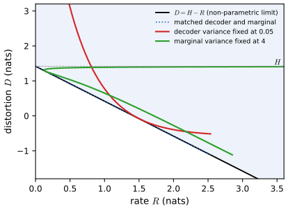
Filling the gap 5.20: the exact slacks in \(H-D\le\MI\le R\), the sum \(D+R\ge H\), and the Gaussian example pp. 248–250, (5.153)–(5.161)
Derivation
Rate. Let \(p(z)=\int p(x)e(z|x)\) (aggregate posterior). \(R=\E_{x,z}\log\frac{e(z|x)}{m(z)}=\E\log\frac{e(z|x)}{p(z)}+\E\log\frac{p(z)}{m(z)}=\MI(x;z)+\Dkl(p(z)\|m(z))\ge\MI(x;z)\), equality iff \(m=p(z)\).
Distortion. \(D=-\E\log d(x|z)=\Hent(x|z)+\E_z\Dkl(p(x|z)\|d(x|z))\ge\Hent(x|z)=H-\MI(x;z)\), so \(H-D\le\MI\), equality iff \(d=p(x|z)\).
Sum. Adding, \(D+R=H+\E_z\Dkl(p(x|z)\|d(x|z))+\Dkl(p(z)\|m)\ge H\): the objective at \(\beta=1\) is bounded below by the data entropy, attained iff decoder and marginal are the true posterior and aggregate posterior, for any encoder: hence all diagonal points have the same ELBO, which is the book's remark that the likelihood cannot choose among them. Also \(-(D+R)=\log p_{\rm model}(x)-\Dkl(e(z|x)\|p_{\rm model}(z|x))\) for the model \(p_{\rm model}(x,z)=m(z)d(x|z)\), the usual ELBO identity. D=0 and R=0 lines: from (5.158), \(D=0\Rightarrow R\ge\MI=H\) (discrete \(x\)); \(R=0\Rightarrow\MI=0\Rightarrow D\ge H\).
Gaussian example. \(x\sim\N(0,1)\), \(z=x+\varepsilon\), \(\varepsilon\sim\N(0,s^2)\): \(p(z)=\N(0,1+s^2)\), \(p(x|z)=\N(\frac z{1+s^2},\frac{s^2}{1+s^2})\), \(R=\MI=\frac12\log\frac{1+s^2}{s^2}\), \(D=\frac12\log\frac{2\pi es^2}{1+s^2}\), so \(D+R=\frac12\log(2\pi e)=H\). With a decoder \(\N(\frac z{1+s^2},v_d)\), \(D=\frac12\log(2\pi v_d)+\frac{s^2}{2v_d(1+s^2)}\); with marginal \(\N(0,v_m)\), \(R=\frac12[\log\frac{v_m}{s^2}+\frac{1+s^2}{v_m}-1]\). Monte Carlo at \(s^2=0.3\) (\(6\times10^5\) draws) matches \(R=0.733\), \(D=0.686\) to 0.005. A random discrete example confirms both slack identities exactly. \(\square\)
5.4.3 Bits back coding
p. 250 Why is the rate \(\E_x\Dkl(e\|m)\) rather than the cross entropy \(\Hce(e(z|x),m)\)? Alice sends \(z\sim e(z|x)\) at cost \(-\log_2m(z)\), then the residual at cost \(-\log_2d(x|z)\): expected \(D+\Hce(e(z|x),m)\) (5.163). Bob decodes \(x\), and since he knows \(z\) and \(e(\cdot|x)\) he can recover the random bits Alice used to sample \(z\) (e.g. bits of a compressed text). Those bits come back, worth \(\Hent(e(z|x))\), leaving \(D+R\) [HC93; FH97]; practical algorithms exist [HPHL19; AT20; TBB19].
Filling the gap 5.21: bits-back accounting p. 250, (5.162)–(5.163)
Derivation
Ideal lengths. Alice samples \(z\) by decoding auxiliary bits \(b\) with an arithmetic decoder for \(e(\cdot|x)\), consuming \(-\log_2e(z|x)\) of them. She transmits \(z\) (cost \(-\log_2m(z)\)) and \(x\) given \(z\) (cost \(-\log_2d(x|z)\)). Bob decodes \(z\), then \(x\), then re-encodes \(z\) with \(e(\cdot|x)\), which returns exactly the consumed bits \(b\). Net cost per image: \(-\log_2m(z)-\log_2d(x|z)+\log_2e(z|x)\), with expectation \(D+\Hce(e,m)-\Hent(e)=D+R\) (5.162, 5.163).
Check. For a random discrete encoder, decoder and marginal, the expected net length equals \(D+R\) exactly, the naive length equals \(D+R+\Hent(e)\), and the difference is \(\Hent(e(z|x))\). By gap 5.20, \(D+R\ge H\), so bits back cannot beat the entropy; it reaches \(-\log p_{\rm model}(x)\) when \(e\) is the model's posterior. Caveats: the auxiliary bits must exist initially (practical schemes use a stack and pay a small start-up cost), and integer-length effects add overhead. \(\square\)
5.5 Error-correcting codes (channel coding)
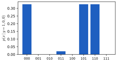
pp. 251–252 Channel coding adds redundancy so a receiver can recover \(\bm x\in\{0,1\}^m\) from a noisy \(\bm y\), e.g. a channel flipping each bit with probability \(\alpha\), \(p(y_i|x_i=0)=[1-\alpha,\alpha]\). The receiver computes \(\argmax_{\bm x}p(\bm x|\bm y)\), combining the channel likelihood with a prior over codewords. With two message bits and an even-parity bit, \(p(\bm x,\bm y)=p(x_1)p(x_2)p(x_3|x_1,x_2)\prod_{i=1}^3p(y_i|x_i)\) (5.164) (Figure 5.11a is a graphical model). For \(\alpha=0.2\) and \(\bm y=(1,0,0)\), the word is not a codeword; the three posterior modes are 000, 110 and 101 (one flip each), and 011 (three flips) is much less likely; 001, 010, 100 are impossible (Figure 5.11b). See Section 9.4.8 for practical codes.
Filling the gap 5.22: the posterior, minimum-distance decoding, and what the capacity says pp. 251–252, (5.164); Fig. 5.11
Derivation
Posterior. \(p(\bm x|\bm y)\propto p(\bm x)\prod_ip(y_i|x_i)\), and for a codeword at Hamming distance \(d\) from \(\bm y\), \(\prod_ip(y_i|x_i)=\alpha^d(1-\alpha)^{3-d}\); the prior is \(\frac14\) on codewords and 0 elsewhere. For \(\bm y=(1,0,0)\): \(d=1\) for 000, 110, 101 (likelihood \(0.2\cdot0.8^2=0.128\)) and \(d=3\) for 011 (\(0.008\)); normalising by \(0.392\) gives 0.3265 and 0.0204.
MAP is minimum distance. For \(\alpha<\frac12\), \(\alpha^d(1-\alpha)^{n-d}\) decreases in \(d\), so MAP decoding with a uniform prior picks the nearest codeword; ties (here three) are unresolvable. The one parity bit detects a single flip but cannot correct it: the exact block error of MAP decoding is 0.36, the same as sending two bits uncoded (\(1-0.8^2\)); a repetition code of length 3 (rate 1/3) has \(3\alpha^2(1-\alpha)+\alpha^3=0.104\).
Capacity. The binary symmetric channel has capacity \(1-\Hent_2(\alpha)=0.278\) bits per use at \(\alpha=0.2\) (Shannon's noisy-channel coding theorem, cited from [CT06]): vanishing error is possible only at rates below it. The rate of the parity code, \(2/3\), is far above, which is why it cannot correct errors; the repetition code's rate \(1/3\) is also above \(0.278\), so its error stays finite. \(\square\)
5.6 The information bottleneck
p. 252 Discriminative models \(p(y|x)\) with a stochastic bottleneck prevent overfitting and improve robustness and calibration.
5.6.1 Vanilla IB
pp. 252–253 A representation \(z\) of \(x\) is a (stochastic) function \(p(z|x)\); it is sufficient for \(y\) if \(y\perp x\mid z\), i.e. \(\MI(z;y)=\MI(x;y)\); minimal sufficient if also \(\MI(z;x)\) is smallest. The information bottleneck [TPB99] optimises over \(p(z|x),p(y|z)\) \[ \min\ \beta\,\MI(z;x)-\MI(z;y),\quad\beta\ge0, \tag{5.165} \] under \(Z\leftarrow X\leftrightarrow Y\), \(p(x,y,z)=p(z|x)p(y|x)p(x)\) (5.166) (Figure 5.12, sketch). For discrete variables the algorithm of [TPB99] applies; for jointly Gaussian variables it is solvable analytically [Che+05] (a supervised PCA); in general it is intractable.
Filling the gap 5.23: the self-consistent equations of the information bottleneck and why the iteration decreases the objective pp. 252–253, (5.165), [TPB99]
Derivation
For any \(p(z|x)\), \(m(z)\), \(r(y|z)\) define \(F=\beta\E_x\Dkl(p(z|x)\|m(z))+\E_{x,z}\Dkl(p(y|x)\|r(y|z))\). Since \(\E_x\Dkl(p(z|x)\|m)=\MI(x;z)+\Dkl(p(z)\|m)\) (gap 5.20) and, using \(p(z,y)=\sum_xp(x)p(z|x)p(y|x)\) (the Markov structure), \(\E_{x,z}\Dkl(p(y|x)\|r)=\MI(x;y)-\MI(z;y)+\E_z\Dkl(p(y|z)\|r(y|z))\), we get \(F\ge\beta\MI(x;z)-\MI(z;y)+\MI(x;y)\), with equality iff \(m=p(z)\), \(r=p(y|z)\). So minimising \(F\) over \((p(z|x),m,r)\) minimises (5.165).
Alternating minimisation. For fixed \(p(z|x)\) the best \(m\) and \(r\) are the marginal \(m(z)=\sum_xp(x)p(z|x)\) and \(r(y|z)=\sum_xp(x|z)p(y|x)\). For fixed \(m,r\), the problem for each \(x\) is \(\min_{p(\cdot|x)}\sum_zp(z|x)[\beta\log\frac{p(z|x)}{m(z)}+\Dkl(p(y|x)\|r(y|z))]\), solved by the Gibbs variational principle: \[ p(z|x)=\frac{m(z)\exp[-\Dkl(p(y|x)\|p(y|z))/\beta]}{Z(x)}. \tag{IB} \] Each step lowers \(F\), which is bounded below, so \(F\) converges; the limit satisfies (IB) with consistent \(m,r\). (In Tishby's convention the multiplier is on \(\MI(z;y)\): \(\beta_T=1/\beta\).) The objective is not convex: the iteration finds a local optimum and depends on the start.
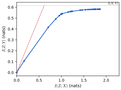
Numerics. On the 12-word, 4-family counts the objective decreases monotonically along the iteration; at a converged solution its gradient in the softmax parameters is \(10^{-10}\); \(\MI(z;y)\le\MI(z;x)\) and \(\le\MI(x;y)=0.614\) nats. With 12 slots the iteration gives the trivial solution above \(\beta\approx1\) and splits into three, four and six clusters as \(\beta\) falls (information plane: Figure 5.S3, and the demo). \(\square\)
5.6.2 Variational IB
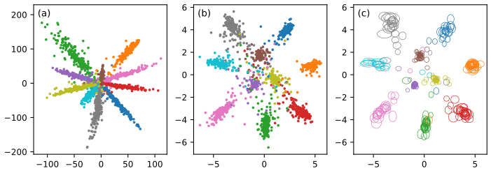
pp. 253–254 With the encoder \(e(z|x)=p(z|x)\), decoder \(d(y|z)\approx p(y|z)\), marginal \(m(z)\approx p(z)\), the bounds \(\MI(z;y)\ge\langle\log d(y|z)\rangle\) (5.168)–(5.172) and \(\MI(z;x)\le\langle\log e(z|x)\rangle-\langle\log m(z)\rangle\) (5.174)–(5.178) give the variational IB (VIB) [Ale+16] \[ \mathcal L_{\rm VIB}=-\E_{p_{\mathcal D}(x)e(z|x)d(y|z)}[\log d(y|z)]+\beta\,\E_{p_{\mathcal D}(x)}\Dkl(e(z|x)\|m(z)), \tag{5.180, 5.181} \] minimised by SGD with the reparameterisation trick. Figure 5.13: an MLP with a 2-D bottleneck on MNIST, deterministic versus stochastic encoder.
Filling the gap 5.24: the VIB bounds with their exact slacks pp. 253–254, (5.167)–(5.181)
Derivation
Lower bound on \(\MI(z;y)\). \(\MI(z;y)=\E\log\frac{p(y|z)}{p(y)}=\E\log d(y|z)+\Hent(y)+\E_z\Dkl(p(y|z)\|d(y|z))\ge\langle\log d\rangle+\Hent(y)\); the book drops the constant \(\Hent(y)\) in (5.170). Slack: the KL between true and variational classifier. (5.167) is \(\E_p\log p\ge\E_p\log q\).
Upper bound on \(\MI(z;x)\). \(\MI(z;x)=\E\log e(z|x)-\E_{p(z)}\log p(z)\), and \(-\E_{p(z)}\log p(z)\le-\E_{p(z)}\log m(z)\) with slack \(\Dkl(p(z)\|m)\); equivalently \(\MI(z;x)=R-\Dkl(p(z)\|m)\), \(R=\langle\log e\rangle-\langle\log m\rangle\).
Combined. \(\beta\MI(x;z)-\MI(z;y)\le\beta R-\langle\log d\rangle-\Hent(y)=\mathcal L_{\rm VIB}-\Hent(y)\) (5.179–5.181), with total slack \(\beta\Dkl(p(z)\|m)+\E_z\Dkl(p(y|z)\|d)\). For a Gaussian encoder, \(\Dkl(\N(\bm\mu,\diag\bm\sigma^2)\|\N(\bm0,\bm I))=\frac12\sum_i(\mu_i^2+\sigma_i^2-1-\log\sigma_i^2)\) in closed form. The marginal \(m\) controls the tightness: a flexible \(m\) (a mixture) approximates the aggregate posterior, a mixture of \(N\) Gaussians for an empirical \(p(x)\). A random discrete example confirms both identities exactly. \(\square\)
5.6.3 Conditional entropy bottleneck
pp. 254–256 The IB can be written \(\min\MI(x;z)-\lambda\MI(y;z)\) (5.182), but \(\MI(z;x)\) contains information relevant to \(y\). The conditional entropy bottleneck [Fis20] minimises only the residual, \[ \min\ \MI(x;z|y)-\lambda'\MI(y;z)\ (5.183),\qquad\text{bounded by}\quad\min\ \beta(\langle\log e(z|x)\rangle-\langle\log b(z|y)\rangle)-\langle\log d(y|z)\rangle\ (5.190), \] with \(b(z|y)\) a backward encoder (easier to learn than the marginal \(m\)); (5.184)–(5.189) give \(\MI(x;z|y)=\MI(x;z)-\MI(y;z)\) and the bound. The book says CEB is IB with \(\lambda'=\lambda+1\) (see the correction below). Figure 5.14 is a sketch.
Filling the gap 5.25: the CEB identity, its bound, and the correct relation to IB pp. 254–256, (5.182)–(5.190)
Derivation
Identity. Under \(z\perp y\mid x\), \(\MI(z;x,y)=\MI(z;x)\); also \(\MI(z;x,y)=\MI(z;y)+\MI(z;x|y)\). So \(\MI(x;z|y)=\MI(x;z)-\MI(y;z)\) (5.184), \(=\Hent(z|y)-\Hent(z|x)\) (5.185–5.186) because \(p(z|x,y)=p(z|x)\).
Bound. \(-\Hent(z|x)=\langle\log e(z|x)\rangle\) exactly, and \(\Hent(z|y)=-\E\log p(z|y)=-\langle\log b\rangle-\E_y\Dkl(p(z|y)\|b(z|y))\). Hence \(\MI(x;z|y)=\langle\log e\rangle-\langle\log b\rangle-\E_y\Dkl(p(z|y)\|b)\le\langle\log e\rangle-\langle\log b\rangle\) (5.188), slack \(\E_y\Dkl(p(z|y)\|b)\); tightest when \(b=p(z|y)\). With \(\MI(x;z|y)=0\) at an optimal representation, the bound's value measures distance from optimality, unlike IB.
Relation to IB. \(\MI(x;z|y)-\lambda'\MI(y;z)=\MI(x;z)-(1+\lambda')\MI(y;z)\), which is the IB objective (5.182) with \(\lambda=1+\lambda'\), i.e. \(\lambda'=\lambda-1\): the book's "\(\lambda'=\lambda+1\)" has the roles reversed. A random discrete example confirms identity and slack. \(\square\)
5.7 Algorithmic information theory
p. 256 Shannon information describes a stochastic source, not a single sequence: \(n\) fair bits have \(-\log_2p=n\) whatever they are, yet "0101..." seems to carry little information. Algorithmic information theory measures a given string (Solomonoff, Kolmogorov, Chaitin) [Hut07; GV08; LV19].
5.7.1 Kolmogorov complexity
pp. 256–257 \(K(x)=\min_p\{\ell(p):U(p)=x\}\) for a universal Turing machine \(U\); it has Shannon-like properties, e.g. \(K(x|y)\le K(x)\le K(x,y)\) up to additive constants. It is not computable; Levin complexity \(L(x)=\min_p[\ell(p)+\log\mathrm{time}(p)]\) is computable via universal search in time \(2^{L(x)}\). For a distribution \(q\) over strings, \(K(x)\le-\log q(x)+K(q)\) (an MDL-type bound). A string is algorithmically random if \(K(x)\ge\ell(x)\) (Martin-Lof); \((10101010\cdots)\) is compressible, the binary digits of \(\pi\) too, and quantum-noise bits are not. Lempel–Ziv compression and the normalised compression distance \(d(x,y)=\frac{\max[K(x|y),K(y|x)]}{\max[K(x),K(y)]}\) (5.191) follow [CV05; Jia+23].
Filling the gap 5.26: invariance, incompressibility counting, uncomputability, and the bound \(K(x)\le-\log q(x)+K(q)+c\) pp. 256–257, (5.191)
Proofs
Invariance. If \(V\) is another universal machine, a fixed interpreter for \(V\) on \(U\) of length \(c_{UV}\) gives \(K_U(x)\le K_V(x)+c_{UV}\) for all \(x\): the choice of language changes \(K\) by a constant (the book's footnote on \(\pi\)).
Counting. There are \(\sum_{l<n-c}2^l=2^{n-c}-1\) programs shorter than \(n-c\) bits, so fewer than \(2^{n-c}\) strings of length \(n\) have \(K(x)<n-c\); a fraction \(\ge1-2^{-c}\) satisfy \(K(x)\ge n-c\): most strings are nearly incompressible. And \(K\) of the repetition \(1010\cdots\) of length \(n\) is \(\le\log n+c\).
Inequalities (up to constants). \(K(x)\le K(x,y)+c\): from a program printing the pair, output its first component; \(K(x|y)\le K(x)+c\): ignore the side information.
Uncomputability. Suppose \(K\) were computable. For each \(m\) let \(P_m\) be: "list strings in length-lexicographic order and print the first \(x\) with \(K(x)\ge m\)". It exists (such strings exist by counting) and describing it needs only \(m\), i.e. \(\ell(P_m)\le\log_2m+c\). It prints \(x_m\) with \(K(x_m)\ge m\), but \(K(x_m)\le\log_2m+c<m\) for \(m\) large: contradiction (Berry's paradox).
Distribution bound. For a computable \(q\), the arithmetic code of gap 5.19 has length \(\le-\log_2q(x)+2\); a program that contains a description of \(q\) (\(K(q)\) bits) and a decoder (a constant) outputs \(x\) from that code: \(K(x)\le-\log_2q(x)+K(q)+c\). For \(q\) a parametric model, \(K(q)\) is the coding length of the parameters: MDL. In expectation under \(q\), \(\E K(x)\approx\Hent(q)+K(q)\).
Numerics (compressors as stand-ins). With zlib: the normalised distance of a random 4000-byte string to itself is 0.021 and to an independent random string 0.997; the compressed length of 200 000 iid Bernoulli(0.1) bits is 131 760 bits against \(N\,\Hent=93\,799\): any compressor stays above the Shannon bound, and a general-purpose one is far from it on iid data. \(\square\)
5.7.2 Solomonoff induction
pp. 257–259 Predict \(x_{t+1}\) given \(x_{1:t}\sim\mu\) with a countable class \(\mathcal M\) of models \(\nu\), weights \(w_\nu\) (Solomonoff: \(\mathcal M\) all computable distributions, \(w_\nu=2^{-K(\nu)}\)), and the Bayes mixture \(\xi(x_{1:t})=\sum_\nu w_\nu\nu(x_{1:t})\) (5.192), with posterior predictive \(\xi(x_t|x_{<t})=\sum_\nu w(\nu|x_{<t})\nu(x_t|x_{<t})\) and \(w(\nu|x_{1:t})=w_\nu\nu(x_{1:t})/\xi(x_{1:t})\) (5.193–5.195). With squared error \(s_t(x_{<t})=\sum_{x_t}(\mu-\xi)^2\) (5.196) and total error \(S_n=\sum_{t\le n}\sum_{x_{<t}}\mu(x_{<t})s_t\) (5.197), Solomonoff proved \[ S_\infty\le\ln w_\mu^{-1}=K(\mu)\ln2. \tag{5.198} \] For deterministic programs, \(M(x)=\sum_{p:U(p)=x*}2^{-\ell(p)}\) (5.199) and \(M=\xi\) [WSH13]. It is uncomputable but can be approximated (e.g. by meta-learned sequence models [GM+24]); [HQC24] builds AIXI on it.
Filling the gap 5.27: the posterior weights and a full proof of \(S_\infty\le\ln w_\mu^{-1}\) pp. 257–259, (5.192)–(5.198)
Proof
Predictive (5.193–5.195). \(\xi(x_t|x_{<t})=\xi(x_{1:t})/\xi(x_{<t})=\sum_\nu\frac{w_\nu\nu(x_{<t})}{\xi(x_{<t})}\nu(x_t|x_{<t})\) and \(\frac{w_\nu\nu(x_{<t})}{\xi(x_{<t})}=w(\nu|x_{<t})\) is the Bayes posterior over models.
Dominance. \(\xi\ge w_\mu\mu\) pointwise (one term of the sum). (For \(\xi\) to be a probability measure \(\sum w_\nu\le1\); for \(w_\nu=2^{-K(\nu)}\) this is Kraft's inequality for prefix complexity.)
Step 1 (KL telescopes). Let \(\mathrm{KL}_t(x_{<t})=\sum_{x_t}\mu(x_t|x_{<t})\ln\frac{\mu(x_t|x_{<t})}{\xi(x_t|x_{<t})}\). By the iterated chain rule (gap 5.2), \(\sum_{t\le n}\E_\mu\mathrm{KL}_t=\Dkl(\mu_{1:n}\|\xi_{1:n})=\E_\mu\ln\frac{\mu(x_{1:n})}{\xi(x_{1:n})}\le\ln w_\mu^{-1}\) by dominance.
Step 2 (squared error \(\le\) KL). For pmfs \(a,b\): (i) Pinsker, \(\Dkl(a\|b)\ge\frac12\|a-b\|_1^2\): let \(A=\{a>b\}\), the channel \(x\mapsto\mathbb 1_A(x)\) and gap 5.7 give \(\Dkl(a\|b)\ge d(\alpha,\beta)\) with \(\alpha=a(A)\), \(\beta=b(A)\), \(d\) the Bernoulli KL; \(g(t)=d(\alpha,t)-2(\alpha-t)^2\) has \(g(\alpha)=0\), \(g'(t)=(t-\alpha)\big(\frac1{t(1-t)}-4\big)\), with the sign of \(t-\alpha\) since \(t(1-t)\le\frac14\), so \(g\ge0\), and \(2(\alpha-\beta)^2=\frac12\|a-b\|_1^2\). (ii) For \(v=a-b\) with \(\sum v=0\), the positive and negative parts each sum to \(\frac12\|v\|_1=P\), so \(\|v\|_2^2\le P^2+P^2=\frac12\|v\|_1^2\). Hence \(\|a-b\|_2^2\le\Dkl(a\|b)\), i.e. \(s_t\le\mathrm{KL}_t\).
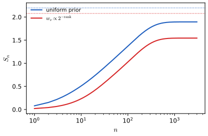
Conclusion. \(S_n\le\sum_t\E_\mu\mathrm{KL}_t\le\ln w_\mu^{-1}\) for all \(n\), so \(S_\infty\le\ln w_\mu^{-1}=K(\mu)\ln2\) when \(w_\mu=2^{-K(\mu)}\). Simple environments are learned quickly in total squared error.
Numerics (Figure 5.S4). Class: nine Bernoulli models \(\theta\in\{0.1,\dots,0.9\}\), truth \(\theta=0.3\). \(S_n\) computed exactly (sums over counts) up to \(n=3000\): with the uniform prior \(S_\infty\approx1.895<\ln9=2.197\); with \(w_\nu\propto2^{-\mathrm{rank}}\) (truth of rank 3) \(S_\infty\approx1.544<2.077\). The bound is not attained here (it is a worst case over the class) but is of the right order. The equality \(M=\xi\) is cited, not proved. \(\square\)
Practice problems
The book has no end-of-chapter exercises for Chapter 5, so here are three short problems of my own, with complete solutions (hidden).
Practice problem 5.1 (weight of evidence). A coin is either fair (\(Q\): \(\theta=0.5\)) or biased (\(P\): \(\theta=0.7\)); the truth is \(P\). (a) Compute \(\Dkl(p\|q)\) and \(\Dkl(q\|p)\) in nats and bits. (b) How many flips are needed for the expected weight of evidence for \(P\) over \(Q\) to reach \(\ln100\)? (c) Bound the probability that the data favour \(Q\) over \(P\) by a likelihood ratio of 100 or more.
Solution
(a) \(\Dkl(p\|q)=0.7\ln1.4+0.3\ln0.6=0.2355-0.1532=0.0823\) nats \(=0.1187\) bits; \(\Dkl(q\|p)=0.5\ln\frac{0.5}{0.7}+0.5\ln\frac{0.5}{0.3}=-0.1682+0.2554=0.0872\) nats \(=0.1258\) bits: not symmetric, but close for such similar coins. (b) \(\E w=n\Dkl(p\|q)\) (gap 5.3), so \(n=\ln100/0.0823=4.605/0.0823\approx56\) flips (53 if the roles were reversed). (c) By the Markov bound of gap 5.3, \(\Pr_p(q(D)/p(D)\ge100)\le1/100\), for any \(n\). \(\square\)
Practice problem 5.2 (a diagonal Gaussian for a correlated pair). \(p=\N(\bm0,\left(\begin{smallmatrix}1&\rho\\\rho&1\end{smallmatrix}\right))\), \(q\) diagonal. For \(\rho=0.9\) find the two optimal \(q\), and the four divergences \(\Dkl(p\|q_f),\Dkl(q_f\|p),\Dkl(p\|q_r),\Dkl(q_r\|p)\).
Solution
\(q_f=\diag(1,1)\) (marginal variances) and \(q_r=\diag(1-\rho^2,1-\rho^2)=\diag(0.19,0.19)\) (inverse diagonal of \(\bm\Lambda=\frac1{1-\rho^2}\left(\begin{smallmatrix}1&-\rho\\-\rho&1\end{smallmatrix}\right)\)) by gap 5.4 and 5.5. Then \(\Dkl(p\|q_f)=\frac12\log\frac{1}{1-\rho^2}=0.8304\) nats \(=\Dkl(q_r\|p)\) (both equal \(\MI\)), and \(\Dkl(q_f\|p)=\Dkl(p\|q_r)=\frac12[\frac{2}{0.19}-2+\ln0.19]=\frac12[10.526-2-1.661]=3.4328\) nats. The "wrong-direction" costs are four times larger than the optimised ones. The demo with preset 1 shows the same numbers. \(\square\)
Practice problem 5.3 (InfoNCE batch size). A Gaussian pair has \(\MI=3\) nats (\(\rho=0.99876\)). With the optimal critic, what is the smallest \(K\) for which \(\MI_{\rm NCE}\) could reach 2.5 nats, and what does InfoNCE actually give at \(K=4,16,64,256\)?
Solution
Since \(\MI_{\rm NCE}\le\log K\) (gap 5.17), reaching 2.5 nats needs \(K\ge e^{2.5}=12.18\), so \(K\ge13\). Monte Carlo estimates with the optimal critic (
infonce_mcin the code, standard errors about 0.007) give 1.28, 2.25, 2.76 and 2.93 nats at \(K=4,16,64,256\), against the caps 1.39, 2.77, 4.16, 5.55: the gap to \(\log K\) is small for small \(K\) and the estimate approaches \(\MI=3\) only slowly (Figure 5.S2). \(\square\)
Demonstrations
| Page | What it shows | In the notes |
|---|---|---|
| Diagonal Gaussian approximations of a correlated Gaussian | Forward and reverse KL projections of a correlated 2-D Gaussian onto diagonal Gaussians, your own \(q\), and the KL over the variance plane. Presets: 1 correlation 0.9; 2 independent; 3 correlation 0.99; 4 unequal scales; 5 negative correlation. | 5.1.4.2, 5.1.4.3, gap 5.4, gap 5.5 |
| Variational bounds on mutual information | Upper, Barber–Agakov, Donsker–Varadhan, NWJ and InfoNCE bounds for a Gaussian pair against the true value. Presets: 1 all tight; 2 shrunken critic; 3 wrong NWJ offset; 4 large information, small batch; 5 poor variational distributions. | 5.3.6, gap 5.17 |
| The information bottleneck on word-class counts | Self-consistent information-bottleneck iteration on twelve words and four newsgroup families, the information-plane curve and the clusters. Presets: 1 one cluster; 2 three clusters; 3 four clusters; 4 six clusters; 5 two slots only. | 5.6.1, gap 5.23 |
The Python code that produces every figure of this page is code/ch05_information_theory.py (see the code index). Data for the bottleneck demo: data/ch05-word-class.json. Companion demos: entropy, cross entropy and KL, forward versus reverse KL.
Notes on the book
Points where the book is imprecise or wrong
- Section 5.2.4, last sentence. The perplexity can never go below \(2^{+\Hent(p^*)}\); the text prints \(2^{-\Hent(p^*)}\), which is at most 1 (gap 5.14).
- Section 5.6.3. "CEB is equivalent to standard IB with \(\lambda'=\lambda+1\)": from \(\MI(x;z|y)=\MI(x;z)-\MI(y;z)\), (5.183) equals (5.182) with \(\lambda=\lambda'+1\) (gap 5.25).
- Supplement (5.5). The quadratic term \((\bm\mu-\bm m)^\T\bm\Sigma(\bm\mu-\bm m)\) should have \(\bm\Lambda=\bm\Sigma^{-1}\); the conclusion \(\bm m=\bm\mu\) is unaffected (gap 5.5).
- Section 5.4.2. In the zero-rate discussion, "the latent code is independent of \(z\)" should read independent of \(x\).
- Section 5.1.6, (5.62)–(5.64). For continuous data \(\Dkl(p_{\mathcal D}\|q)\) is \(+\infty\) and \(C=-\infty\); the identities hold for the cross entropy (gap 5.8).
- Section 5.3.6.3, (5.147)–(5.148). The bound with \(\E_{p(y)}\log Z(y)\) is valid and tighter than the usual single-logarithm Donsker–Varadhan bound; the name refers to the latter in the literature (gap 5.17). NWJ is tight at \(f=1+\log\) ratio, not at the log ratio.
- Section 5.5. "(if \(x_1=1\) then we know \(x_3=1\))" holds only when \(x_2=0\), since \(x_3=x_1\oplus x_2\); the reason \(y=(1,0,0)\) is not a codeword is that it has odd parity.
References
- Murphy, K. P. (2023). Probabilistic Machine Learning: Advanced Topics. MIT Press, Cambridge, MA. Chapter 5, pp. 219–259, and supplementary material, Chapter 5. probml.github.io/pml-book/book2.html.
- Barber, D. and Agakov, F. (2003). The IM algorithm: a variational approach to information maximization. Advances in Neural Information Processing Systems, 16.
- Cover, T. M. and Thomas, J. A. (2006). Elements of Information Theory, 2nd edition. Wiley, New York.
- Fischer, I. (2020). The conditional entropy bottleneck. Entropy, 22(9), 999.
- Alemi, A. A., Fischer, I., Dillon, J. V. and Murphy, K. (2016). Deep variational information bottleneck. International Conference on Learning Representations.
- Hinton, G. E. and van Camp, D. (1993). Keeping the neural networks simple by minimizing the description length of the weights. Proceedings of COLT.
- Hutter, M. (2007). Universal algorithmic intelligence. In Artificial General Intelligence, Springer.
- Li, M. and Vitanyi, P. (2019). An Introduction to Kolmogorov Complexity and Its Applications, 4th edition. Springer.
- Nguyen, X., Wainwright, M. J. and Jordan, M. I. (2010). Estimating divergence functionals and the likelihood ratio by convex risk minimization. IEEE Transactions on Information Theory, 56(11), 5847–5861.
- Oord, A. van den, Li, Y. and Vinyals, O. (2018). Representation learning with contrastive predictive coding. arXiv:1807.03748.
- Poole, B., Ozair, S., van den Oord, A., Alemi, A. A. and Tucker, G. (2019). On variational bounds of mutual information. International Conference on Machine Learning.
- Renyi, A. (1961). On measures of entropy and information. Proceedings of the Fourth Berkeley Symposium, 1, 547–561.
- Solomonoff, R. J. (1964). A formal theory of inductive inference. Information and Control, 7(1–2), 1–22 and 224–254.
- Tishby, N., Pereira, F. C. and Bialek, W. (1999). The information bottleneck method. Proceedings of the 37th Allerton Conference.
- White, H. (1982). Maximum likelihood estimation of misspecified models. Econometrica, 50(1), 1–25.
The numerical statements in the text (the desiderata and chain rule, the projections onto diagonal Gaussians, the compression lemma, data processing, the exponential-family and Bregman identities, the Fisher approximation, the entropy units, typical sets, the mutual-information identities and bounds, the coding results, the rate–distortion and bottleneck identities, and the Solomonoff bound) were confirmed numerically.