Beyond the iid assumption
Supervised learning is usually analysed as if the training and test examples were independent draws from one distribution. This chapter asks what happens when they are not. A model fitted to \(p(x,y)\) is run on \(q(x,y)\): which part of the distribution moved (the covariates, the labels, the concept, the way a label shows itself), how to notice it, how to make the model robust to it, how to adapt with or without target labels, how to learn from many distributions at once, how to keep learning as the distribution keeps changing, and how an adversary can pick the shift on purpose. The notes prove the claims the book states without proof (importance weighting, the density-ratio classifier, blackbox shift estimation, the marginal-entropy objective, the meta-learning objective, the regret of online gradient descent, the exact adversarial attack on a linear model, randomised smoothing, the concentration-of-measure distance), and reproduce the computed figures with my own code.
Ch. 1 Introduction Ch. 2 Probability Ch. 3 Statistics Ch. 4 Graphical models Ch. 5 Information theory Ch. 6 Optimisation Ch. 7 Inference algorithms Ch. 8 Gaussian filtering Ch. 9 Message passing Ch. 10 Variational inference Ch. 11 Monte Carlo Ch. 12 MCMC Ch. 13 Sequential Monte Carlo Ch. 14 Predictive models Ch. 15 GLMs Ch. 16 Deep networks Ch. 17 Bayesian neural networks Ch. 18 Gaussian processes Ch. 19 Beyond iid Ch. 20 Generative models Ch. 21 VAEs Ch. 22 Autoregressive models Ch. 23 Normalizing flows Ch. 24 Energy-based models Ch. 25 Diffusion models Ch. 26 GANs Ch. 27 Discovery methods Ch. 28 Latent factor models Ch. 29 State-space models Ch. 30 Graph learning Ch. 31 Nonparametric Bayes Ch. 32 Representation learning Ch. 33 Interpretability Ch. 34 Decision making Ch. 35 Reinforcement learning Ch. 36 Causality
How to read these notes
They follow the book. Sections carry the book's numbers, and I keep the book's equation numbers where I restate an equation, e.g. (19.16), (19.22), (19.52). The chapter is a survey: most of its mathematics is stated in a line or quoted from a paper, so most of the work here is in the gap boxes.
Filling the gaps. Wherever the book asserts a result without proof (that selection on \(X\) or \(Y\) gives covariate or label shift, the importance-weighting identity and its variance, the logistic-regression density ratio, the domain-adaptation objective, blackbox shift estimation, the marginal-entropy objective, the meta-learning objective, the regret bound, the fast gradient sign step, the equation (19.52)), an orange Filling the gap box gives the full argument. Proofs start hidden; click a bar to open one.
Figures. Figures 19.4, 19.8, 19.9 and 19.10 are reproduced from simulation or from small networks trained here. Figures 19.1 and 19.7 are replaced by stand-ins of my own, because the book's versions need a pretrained ResNet-50 and a Glow model on CIFAR-10 (the captions say so). Figures 19.28 to 19.34 are my own, for topics the book only describes: label shift, invariant risk minimisation, continual learning (the real version of the schematic Figures 19.20 and 19.21), online learning, adversarial attacks on a linear classifier and the concentration of measure. The photographs and diagrams (19.2, 19.3, 19.5, 19.6, 19.11 to 19.19, 19.22 to 19.26, 19.27b) contain nothing computed and are not reproduced.
Main reference
K. P. Murphy, Probabilistic Machine Learning: Advanced Topics, MIT Press (2023; December 2025 draft), Chapter 19, pages 735–770 (book page: probml.github.io/pml-book/book2.html). The explanations, derivations, figures and code are my own.
Companion courses
- Probabilistic Machine Learning: An Introduction: Chapter 19 (learning with fewer labels) covers data augmentation, fine-tuning, domain adaptation, MAML and few-shot learning from the first-volume point of view; Chapter 10 has the logistic regression used for the density ratio.
- All of Statistics: Chapter 16 (causal inference) for the causal language of 19.2.2 and the selection variable of 19.2.4.
- Foundations of Deep Learning: 10.3.4 adversarial attacks and Chapter 9 (regularization) for the network-side view of 19.4 and 19.8.
- This course: gap 11.8 (self-normalised importance sampling, effective sample size) is the machinery behind 19.5.2; 2.7.5 (density ratio by a classifier); 12.7.1 (stochastic gradient Langevin dynamics) for Figures 19.8 and 19.9; 14.3 conformal prediction for 19.3.2.3; 10.1.5 amortized inference for 19.6.4.1; 4.2.4 (selection bias, colliders). Chapter 17 (Bayesian neural networks, elastic weight consolidation) and Chapter 36 (causality) continue from here.
What this chapter adds: the exact form of every statement the book makes in a sentence (the variance and effective sample size of importance weighting, the finite-sample error of blackbox shift estimation, the exact worst-case perturbation of a linear classifier and the closed form of its adversarial training, the Neyman-Pearson proof of the smoothing radius), plus small experiments on the claims the book illustrates with large models.
The chapter at a glance
- 19.2 Four ways \(p\to q\) can move (covariate, concept, label, manifestation) and how sampling creates a shift (gap 19.1).
- 19.3 Noticing a shift: two-sample tests, OOD scores (gap 19.2, gap 19.3), selective prediction with plug-in and Bayesian networks.
- 19.4 Robustness: augmentation is a regulariser (gap 19.4); distributionally robust optimisation is a worst-case weighted ERM (gap 19.5).
- 19.5 Adaptation: fine-tuning (gap 19.6), importance weights (gap 19.7, gap 19.8), domain-adversarial learning (gap 19.9), blackbox label-shift estimation (gap 19.10), test-time entropy minimisation (gap 19.11).
- 19.6 Many distributions: invariant risk minimisation on an exact toy (gap 19.12), meta-learning objectives (gap 19.13, gap 19.14).
- 19.7 Continual and online learning: sequential Bayes and elastic weight consolidation (gap 19.15), prequential evaluation (gap 19.16), regret (gap 19.17).
- 19.8 Adversarial examples: the exact attack on a linear model (gap 19.18), adversarial training and Danskin's theorem (gap 19.19), randomised smoothing (gap 19.20), and why they exist in high dimension (gap 19.21).
Notation. \(p\) is the source and \(q\) the target distribution; \(\ell\) a loss; \(R(f,q)=\E_q[\ell(y,f(x))]\) the target risk; \(w(x)=q(x)/p(x)\) the density ratio; \(\Phi,\Phi^{-1}\) the standard normal cdf and its inverse; \(\|\cdot\|_p\) the \(\ell_p\) norm and \(\|\cdot\|_{p'}\) its dual norm.
19.1 Introduction
p. 735 The standard recipe of supervised learning assumes that the training and the test examples are independent draws from the same distribution (iid). Real deployments break this in several ways, and the book organises the chapter by how. The test distribution may differ from the training distribution (distribution shift, 19.2, with ways to detect it, 19.3, resist it, 19.4, and adapt to it, 19.5). Data may come from several related distributions rather than two (19.6). Data may stream in while the distribution drifts continuously or in jumps (19.7). Or the test inputs may be chosen by an adversary who wants the predictor to fail (19.8).
19.2 Distribution shift
p. 735 Let the model be trained on labelled data from a source distribution \(p(x,y)\) and used on a target distribution \(q(x,y)\). If \(p\ne q\) there is a distribution shift (or dataset shift). The aim of 19.3 is to notice that \(q\ne p\) and abstain; of 19.4 to build a model that approximates \(q(y\given x)\) while seeing only \(p\); of 19.5 to adapt using some labelled or unlabelled target data.
19.2.1 Motivating examples
pp. 735–736 Small changes to the input distribution can wreck a good classifier. The book's Figure 19.1 shows a ResNet-50 trained on ImageNet losing accuracy as Gaussian noise of growing size is added to the images, and Figure 19.2 shows a vision system calling a cow on a beach a generic mammal because, in its training data, cows stood on grass. The root cause in both cases is that a discriminative model uses any feature that predicts the label in the training set, including spurious correlations or shortcut features (grass, a hospital's metal token on a chest X-ray) that are not stable across distributions.
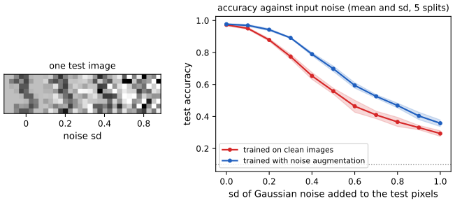
Neither of those experiments is feasible here (a pretrained ResNet-50 and photographs), so Figure 19.1 is replaced by a stand-in of the same kind on a small problem: a one-hidden-layer network trained on the \(8\times8\) digits, then tested with Gaussian noise of growing standard deviation added to the pixels (scaled to \([0,1]\)). Accuracy falls from 97% to about 30% as the noise sd goes from 0 to 1; a network trained on noisy copies of the training images (data augmentation, 19.4.1) degrades more slowly but still degrades.
19.2.2 A causal view of distribution shift
pp. 737–738 Following the causal-inference literature the book classifies a prediction problem by whether the covariates \(X\) cause the label \(Y\) (causal or discriminative prediction, \(X\to Y\)) or the label causes the covariates (anticausal or generative prediction, \(Y\to X\)). A segmentation produced from an image is \(X\to Y\); a disease state that shows on a scan, or a star rating that shapes the words of a review, is \(Y\to X\). The two give the two factorisations \[ p_\theta(x,y)=p_\psi(x)\,p_w(y\given x)\qquad\text{(discriminative)},\tag{19.1} \] \[ p_\theta(x,y)=p_\pi(y)\,p_\phi(x\given y)\qquad\text{(generative)}.\tag{19.2} \] In each factorisation either factor may change from source to target, which gives four canonical shifts. (The graphical models of Figure 19.3, with the source and target parameters, the labelled and unlabelled sets and the loss, are diagrams and are not reproduced.)
19.2.3 The four main types of distribution shift
pp. 738–739 Table 19.1 lists them. For a discriminative model: covariate shift (or domain shift) changes \(p(x)\) and keeps \(p(y\given x)\); concept shift (or annotation shift) keeps \(p(x)\) and changes \(p(y\given x)\). For a generative model: label shift (prior or prevalence shift) changes \(p(y)\) and keeps \(p(x\given y)\); manifestation shift (conditional shift) keeps \(p(y)\) and changes \(p(x\given y)\).
| Name | Source | Target | Model |
|---|---|---|---|
| covariate / domain shift | \(p(X)p(Y\given X)\) | \(q(X)p(Y\given X)\) | discriminative |
| concept shift | \(p(X)p(Y\given X)\) | \(p(X)q(Y\given X)\) | discriminative |
| label (prior) shift | \(p(Y)p(X\given Y)\) | \(q(Y)p(X\given Y)\) | generative |
| manifestation shift | \(p(Y)p(X\given Y)\) | \(p(Y)q(X\given Y)\) | generative |
Covariate shift is the case of a clean training set against noisy, cluttered or synthetic test inputs; the standard remedies are importance weighting (19.5.2) and domain adaptation (19.5.3). Concept shift is a change in what a label means (a different annotation convention, or a new label); since it changes the meaning of a label, it cannot be repaired without labelled target examples, which define the label by example. Label shift is a change in prevalence, as between an urban and a rural hospital; the remedy is to reweight the classifier's output by the new prior (19.5.4). Manifestation shift is the converse of concept shift: the same disease looks different, usually because a hidden factor (the patients' age) changed.
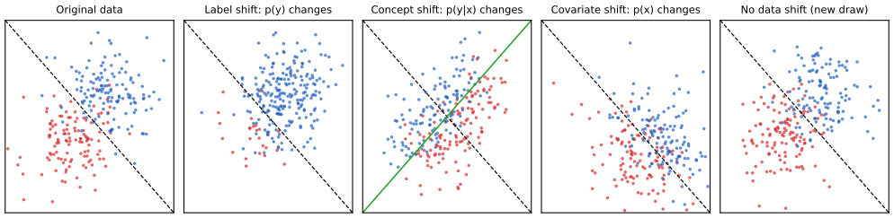
Figure 19.4 shows the four shifts on a two-dimensional binary problem that I simulate so that each one is exact: the source has \(x\given y\sim\N(\pm\mu,I)\) with equal priors, so that \(p(y=1\given x)=\sigma(2\mu^\T x)\). Label shift changes \(P(y=1)\) to 0.9 and leaves \(p(x\given y)\); concept shift rotates the boundary normal by 90 degrees (green line) with the source inputs; covariate shift moves and widens the input cloud and keeps \(p(y\given x)\); the last panel is a fresh draw from the source.
See also: Introduction volume, 19.2.5 domain adaptation.
19.2.4 Selection bias
p. 740 A shift can also arise from how the data were collected, with no change in the world. Let \(S=1\) if a unit from the population enters the training set. The source is \(p(X,Y)=P(X,Y\given S=1)\) and the target is the unselected population \(q(X,Y)=P(X,Y)\). The book distinguishes four mechanisms by what the selection variable depends on (Figure 19.5): none; selection on \(X\) (image quality, a pattern), which induces covariate shift; selection on \(Y\) (oversampling the rare class), which induces label shift; and selection on both, which makes \(X\) and \(Y\) dependent in the selected sample in a way they are not in the population, the selection bias of Section 4.2.4.
Filling the gap 19.1: what each kind of selection does to the distribution p. 740
Derivation
Write \(\pi(x,y)=P(S=1\given X=x,Y=y)\) for the inclusion probability. Bayes' rule gives the selected joint \[ p(x,y)=P(x,y\given S=1)=\frac{\pi(x,y)\,q(x,y)}{P(S=1)},\qquad P(S=1)=\int \pi\,q . \] (a) Selection on \(X\) only, \(\pi=\pi(x)\) (so \(S\perp Y\given X\)). Then \(p(x,y)\propto\pi(x)q(x)q(y\given x)\), so \(p(y\given x)=q(y\given x)\) and \(p(x)\propto\pi(x)q(x)\): the input marginal changes and the conditional does not, which is covariate shift, with density ratio \(q(x)/p(x)=P(S=1)/\pi(x)\) (the reciprocal of the inclusion probability, up to a constant). This is why inverse-probability weights repair selection on \(X\) (19.5.2).
(b) Selection on \(Y\) only, \(\pi=\pi(y)\) (so \(S\perp X\given Y\)). Then \(p(x,y)\propto\pi(y)q(y)q(x\given y)\), so \(p(x\given y)=q(x\given y)\) and \(p(y)\propto\pi(y)q(y)\): the label prior changes and the class-conditional does not, which is label shift, with \(q(y)/p(y)=P(S=1)/\pi(y)\). Balancing a data set by keeping all the rare examples and a fraction of the common ones is of this type, and (19.23) below undoes it.
(c) Selection on both. Take \(X\) and \(Y\) independent in the population, \(q(x,y)=q(x)q(y)\), and \(\pi(x,y)=\ind(x+y>c)\). The selected density is proportional to \(q(x)q(y)\ind(x+y>c)\), supported on the half-plane \(\{x+y>c\}\), which is not a product set, so it cannot factorise as \(p(x)p(y)\): \(X\) and \(Y\) are dependent in the selected sample although independent in the population (\(S\) is a collider, Section 4.2.4). For two standard normals the selected correlation is negative; my simulation with \(c=1\) gives \(-0.62\) against \(0.00\) in the population. A model trained on the selected data will use \(X\) to predict \(Y\) and will be wrong on the population, an unconditional (non-causal) dependence created by the sampling.
See also: 4.2.4 selection bias and colliders; All of Statistics, Chapter 16.
19.3 Detecting distribution shifts
pp. 740–741 No model can be made robust to every shift, and test samples are rarely available at training time. A weaker goal is to detect that a shift has happened and respond, for example by abstaining. The methods split by whether a set of target samples or a single sample is available and whether the target is labelled.
19.3.1 Detecting shifts using two-sample testing
p. 741 Given samples from source and target, the null hypothesis \(p(x,y)=q(x,y)\) (or \(p(x)=q(x)\) for unlabelled samples) is an ordinary two-sample testing problem, for which the book suggests the maximum mean discrepancy (Section 2.7.3, 2.7) on the inputs or Euclidean distances in the embedding space of a classifier trained on the source. Two further routes: if label shift is the only possible change (\(q(x\given y)=p(x\given y)\)) then \(p(y)=q(y)\) suffices to conclude \(q(x,y)=p(x,y)\), and the label distribution can be estimated by the blackbox shift estimator of 19.5.4, which works for detection even when the assumption is violated (Rabanser, Guennemann and Lipton, 2019); and conformal prediction gives distribution-free tests of covariate shift from a calibration set (Hu and Lei, 2020). A classifier two-sample test (train a domain classifier, test whether its held-out accuracy exceeds one half) is the practical counterpart of the density-ratio classifier of gap 19.8, and the optimal discriminator's loss is a function of the Jensen-Shannon divergence (gap 19.9).
19.3.2 Detecting single out-of-distribution (OOD) inputs
p. 741 With one unlabelled target input \(x\sim q\) the question is whether \(x\) is in-distribution (ID) or out-of-distribution (OOD): OOD detection, also called anomaly or novelty detection. (This differs from outlier detection, where one data set is scanned for untypical points, a transductive task.) Often an ID input must in addition be classified, as in the two-stage decision of Figure 19.6 (a diagram, not reproduced).
19.3.2.1 Supervised ID/OOD methods (outlier exposure)
p. 741 If labelled OOD examples ("known unknowns") are available at training time, a binary ID-versus-OOD classifier can be trained against the labelled ID data ("known knowns"). This outlier exposure works well but needs OOD data that cover what will occur, which is rarely possible since OOD is everything except the ID set.
19.3.2.2 Classification confidence methods
p. 742 Instead of a binary decision one can derive an uncertainty score from the class probabilities \(p_c=p(y=c\given x)\): the maximum probability \(s=\max_cp_c\), the margin between the largest and second-largest log probabilities, the entropy \(H(p_{1:C})\), or the energy score. Vaze et al. (2022) and the work they cite find that the plain maximum-probability baseline is hard to beat. Entropy is criticised because it confuses "which of the \(C\) classes?" with "is any class right?". About the energy score, see Notes on the book, item 1: the energy of Liu et al. (2020) is the negative log-sum-exp of the unnormalised logits, not a sum of log probabilities.
19.3.2.3 Conformal prediction
pp. 742–743 Angelopoulos et al. (2021) combine OOD detection with classification and a provable risk bound. The prediction set is \[ T_\lambda(x)=\begin{cases}\varnothing&\text{if }\mathrm{OOD}(x)>\lambda_1\\ \mathrm{APS}(x)&\text{otherwise,}\end{cases}\tag{19.3} \] where \(\mathrm{OOD}(x)\) is a heuristic OOD score (such as one minus the maximum class probability) and \(\mathrm{APS}(x)\) is the adaptive prediction set of 14.3.1: the smallest set of top classes whose probabilities sum above \(\lambda_2\). The thresholds are chosen on a calibration set of ID data only, so as to control \[ R_1(\lambda)=p(T_\lambda(x)=\varnothing),\qquad R_2(\lambda)=p\big(y\notin T_\lambda(x)\given T_\lambda(x)\ne\varnothing\big),\tag{19.4, 19.5} \] the probability of falsely flagging an ID input as OOD (type-I error) and the miss rate among the inputs that are classified. The aim is \(\lambda_1\) as large as possible subject to \(R_1\le\alpha\) (for example no more than 10% of ID inputs flagged), then \(\lambda_2\) as in 14.3.1.
Filling the gap 19.2: why a calibration quantile controls the false-OOD rate pp. 742–743
Derivation
The book defers the argument to the paper. The type-I part is a one-line exchangeability argument, which I prove; the joint control of \(R_1\) and \(R_2\) over two thresholds needs the multiple-testing machinery of the paper ("learn then test") and I only state it.
Claim. Let \(s_1,\dots,s_n\) be the OOD scores of \(n\) calibration inputs and \(s_{n+1}\) the score of a fresh input, all ID and exchangeable (for instance iid), with no ties (almost sure for a continuous score). Let \(\lambda_1\) be the \(k\)-th smallest calibration score with \(k=\lceil(n+1)(1-\alpha)\rceil\) (and \(\lambda_1=\infty\) if \(k>n\)). Then \(\alpha-\frac1{n+1}<P(s_{n+1}>\lambda_1)\le\alpha\).
Proof. By exchangeability the rank of \(s_{n+1}\) among the \(n+1\) scores is uniform on \(\{1,\dots,n+1\}\). The event \(s_{n+1}>\lambda_1\) happens exactly when the rank of \(s_{n+1}\) exceeds \(k\) (it must be larger than the \(k\)-th smallest calibration value, hence at least \(k+1\)), which has probability \((n+1-k)/(n+1)=1-k/(n+1)\). Since \((n+1)(1-\alpha)\le k<(n+1)(1-\alpha)+1\), this lies in \((\alpha-\frac1{n+1},\alpha]\). \(\square\)
So \(R_1(\lambda)\le\alpha\) holds for every sample size, not only asymptotically, and \(\lambda_1\) is as large as the guarantee allows up to the \(1/(n+1)\) slack. It is a statement about ID inputs only: it controls false alarms and says nothing about the detection rate on OOD inputs, which depends on the score. A simulation with \(n=100\), \(\alpha=0.1\) gives a false-flag rate of 0.0997 (the exact value is \(1-91/101=0.0990\)).
See also: 14.3.1 conformalizing classification.
19.3.2.4 Unsupervised methods
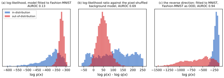
pp. 743–744 Without labels, fit a density model \(p(x)\) to the ID data (a VAE, a flow, an autoregressive model) and flag inputs of low likelihood. Surprisingly, deep generative models trained on Fashion-MNIST give higher likelihood to MNIST digits, and a Glow model trained on CIFAR-10 gives higher likelihood to SVHN than to held-out CIFAR-10 (the book's Figure 19.7). The book's explanation: natural data lie near a low-dimensional manifold and simple data need fewer dimensions, so models defined on the whole ambient space put more density on them. One fix is to use the log-likelihood ratio to a baseline density \(q\), \[ R(x)=\log p(x)-\log q(x), \] instead of \(L(x)=\log p(x)\) (Ren et al., 2019; in the book the baseline is also called \(q\), which I keep, although \(q\) stands for the target elsewhere in the chapter). Its advantage is invariance to invertible transformations \(x'=\phi(x)\): by the change of variables \(p(x')=p(x)\,|\det\mathrm{Jac}(\phi^{-1})(x')|\), so \(L(x')\) differs from \(L(x)\) by a log-Jacobian that depends on the transformation, while the Jacobians cancel in \(R(x')=R(x)\) (the book's (19.6)). Other fixes use a complexity measure (the length of a lossless compression of the input) or the likelihood of features instead of inputs; a reconstruction error from an autoencoder suffers from the same problem as likelihoods; a GAN discriminator can be used for open-set recognition (OpenGAN).
Filling the gap 19.3: why simpler OOD data can have higher likelihood, and what the ratio does pp. 743–744
Derivation
(i) The mode is not the typical set. Let the ID model be \(p=\N(0,I_d)\), so \(\log p(x)=-\frac d2\log2\pi-\frac12\|x\|^2\). For ID data \(x\sim p\), \(\|x\|^2\sim\chi^2_d\) has mean \(d\) and standard deviation \(\sqrt{2d}\), so the average log-likelihood is \(-\frac d2(\log2\pi+1)\). For OOD data \(x\sim\N(0,s^2I_d)\), \(\|x\|^2=s^2\chi^2_d\), and \[ \E\log p(x)=-\tfrac d2\big(\log2\pi+s^2\big),\qquad \mathrm{sd}\,[\log p(x)]=s^2\sqrt{d/2}. \] For \(s<1\) the OOD average exceeds the ID average by \(\frac d2(1-s^2)\), which is of order \(d\), while the standard deviations (\(\sqrt{d/2}\) for ID data, \(s^2\sqrt{d/2}\) for OOD data) are only of order \(\sqrt d\). So the gap-to-spread ratio grows like \(\sqrt d\) and the likelihood separates the two sets in the wrong direction with probability tending to one: with \(d=200\) and \(s=0.8\) the area under the ROC curve for "likelihood says ID" is 0.001 in my simulation (the mean values are \(-247.8\) against \(-283.8\)). The reason is geometric: a high-dimensional Gaussian puts almost all its mass on a thin shell of radius \(\sqrt d\) far from its mode, so a sample from a narrower distribution lies nearer the mode and has higher density although it is far less probable under \(p\) in the sense of belonging to its typical set. Density is not a measure of typicality. The same mechanism, with a model that spends a lot of capacity on local pixel correlations, is what the book refers to as simpler data receiving higher likelihood.
(ii) A real-data version. For an independent-pixel Bernoulli model with rates \(\theta_i\), \(\log p(x)=\sum_i\log(1-\theta_i)+\sum_ix_i\log\frac{\theta_i}{1-\theta_i}\). When most rates are below one half, each ink pixel (\(x_i=1\)) lowers the log-likelihood, so images with less ink score higher whatever their content. Binarised Fashion-MNIST has about 32% ink pixels and MNIST about 13%, so a model fitted to Fashion-MNIST gives MNIST higher likelihood: my AUROC for detecting MNIST as OOD from the log-likelihood is 0.13, worse than chance by a wide margin, while the reverse direction (fitted to MNIST, Fashion-MNIST as OOD) has AUROC 0.94, the asymmetry the book reports for deep models. This is Figure 19.34 below.
(iii) The ratio and invariance. If \(x'=\phi(x)\) is invertible and differentiable, \(p'(x')=p(\phi^{-1}(x'))\,|J(x')|\) with \(J=\det\mathrm{Jac}(\phi^{-1})\), and the same for \(q\). Then \(R(x')=\log p'(x')-\log q'(x')=\log p(x)+\log|J|-\log q(x)-\log|J|=R(x)\). I confirm numerically with \(\phi(x)=\sinh x\) applied to each coordinate: \(L\) changes by \(-\frac12\sum_i\log(1+x_i'^2)\) while \(R\) is unchanged to \(10^{-12}\). What the ratio does not do: invariance says the score does not depend on the coordinates, not that it detects anything: \(R\) separates ID from OOD only if \(q\) captures what ID and OOD have in common (the "background"), so that it cancels. With \(q\) a pixel-shuffled model (one rate shared by all pixels, the Bernoulli model fitted to pixel-shuffled images) the AUROC rises from 0.13 to 0.69, an improvement but far from perfect; with the wrong background it can be worse. For two Gaussians the ratio is a quadratic function of the distance from the mean, so it cannot cure the effect in (i) either.
19.3.3 Selective prediction
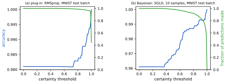
p. 744 If the system has a confidence \(p\) that an input is in-distribution (or that its prediction is right), it can abstain below a threshold, trading accuracy against the abstention rate. This is selective prediction, useful where an error costs more than asking a human (medical imaging). The relevant curves plot, against the threshold \(t\in[0,1]\), the accuracy on the retained inputs and the fraction retained.
19.3.3.1 Example: SGLD vs SGD for MLPs
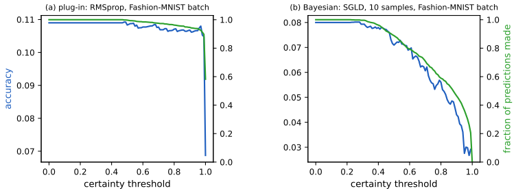
pp. 744–745 Being Bayesian about the weights should improve selective prediction, because the posterior predictive averages over networks that disagree away from the data. The book fits a shallow MLP to MNIST with RMSprop (a plug-in point estimate) or stochastic gradient Langevin dynamics (SGLD, 12.7.1, a form of MCMC), for 6000 steps of minibatch 1000, evaluates on one test batch, and then on a Fashion-MNIST batch as a distribution shift.
My implementation. A 784-100-10 ReLU network on the 60,000 MNIST training images, 6000 minibatch steps of size 1000. Plug-in: RMSprop on the mean cross-entropy (learning rate \(10^{-3}\)). Bayesian: SGLD, \(\theta\leftarrow\theta+\frac\epsilon2\big[\nabla\log\pi(\theta)+N\nabla_{\text{batch}}\log p(\text{batch}\given\theta)\big]+\sqrt\epsilon\,\xi\) with \(\xi\sim\N(0,I)\), \(N=60000\), a \(\N(0,1)\) prior on every weight and \(\epsilon=3\times10^{-6}\); ten parameter snapshots, spaced every 100 steps over the last 1000, form the posterior predictive (average of ten softmax vectors). I tuned \(\epsilon\) only until the chain was stable and reached good accuracy.
Results. On the MNIST test batch the plug-in network has accuracy 98.1% and the SGLD ensemble 96.1% (the book also finds SGD slightly more accurate): SGLD is a short chain and has not converged to the same sharpness. The difference shows on shifted data (Figure 19.9). On 1000 Fashion-MNIST images the "accuracy" against the Fashion labels is meaningless by construction (the classes mean different things; it is near chance, 11% for SGD and 8% for SGLD), but the confidence is informative. At threshold 0.5 the plug-in network still predicts on 99.7% of the images and the Bayesian one on 88.8%; at threshold 0.9, on 94.6% and 46.5%; at 0.99, on 89.7% and 20.6%. So the Bayesian predictor abstains far more on inputs it should not classify, in the direction the book reports (its 97% against 70% at threshold 0.5 comes from a longer or differently tuned chain; the size of the gap depends on the chain length and the prior).
See also: 12.7.1 SGLD. Chapter 17 (Bayesian neural networks), Section 17.4.6.2, studies the behaviour under distribution shift in more depth.
19.3.4 Open set and open world recognition
p. 745 If the lack of confidence is traced to the input belonging to a new class, rather than being an odd instance of a known class, the task is open set recognition (Geng, Huang and Chen, 2020). Instead of flagging such inputs one can let the class set grow, which is open world classification (Bendale and Boult, 2015) and is most natural inside a continual-learning system (19.7). Salehi et al. (2022) survey the link between open-set learning and OOD detection.
19.4 Robustness to distribution shifts
p. 745 Given labelled data from \(p(x,y)\) only, the goal is a model that approximates \(q(y\given x)\) for shifts we cannot see at training time.
19.4.1 Data augmentation
p. 746 The simplest approach is to simulate target data by transforming source data in ways that should not change the label: shifts and rotations of images, replacing "he" by "she" in a sentiment task, back-translation for paraphrases (Shorten and Khoshgoftaar, 2019; Feng et al., 2021). Figure 19.1 (above) shows the effect in the stand-in experiment: training on noisy copies flattens the loss of accuracy against test noise, though it does not remove it. The mathematical content of augmentation with noise is a regulariser.
Filling the gap 19.4: augmenting with noise is a ridge penalty p. 746
Derivation
Take a linear model with squared loss and augment each input with independent noise \(\varepsilon\sim\N(0,\sigma^2I)\), \(\tilde x=x+\varepsilon\). Averaging over the augmentation, for every training pair \((x,y)\), \[ \E_\varepsilon\big[(y-w^\T(x+\varepsilon))^2\big]=(y-w^\T x)^2-2(y-w^\T x)\,w^\T\E\varepsilon+\E\big[(w^\T\varepsilon)^2\big]=(y-w^\T x)^2+\sigma^2\|w\|^2, \] because \(\E\varepsilon=0\) kills the cross term and \(\E[(w^\T\varepsilon)^2]=w^\T\sigma^2Iw\). Hence empirical risk minimisation over infinitely many noisy copies is ridge regression with penalty \(\lambda=N\sigma^2\) on the sum of squares (Bishop, 1995). A Monte Carlo check with \(\sigma=0.35\) gives \(0.7394\) for the simulated average against \(0.7399\) for the formula.
For a general smooth loss \(\ell(y,w^\T x)\), a second-order Taylor expansion in \(\varepsilon\) gives \(\E\,\ell(y,w^\T(x+\varepsilon))\approx\ell(y,w^\T x)+\frac{\sigma^2}2\|w\|^2\,\partial^2_a\ell(y,a)\big|_{a=w^\T x}\): a penalty \(\|w\|^2\) weighted by the curvature of the loss at that example, so noise augmentation penalises the weights most where the loss is most sensitive. The penalty shrinks the weights on directions that are small in the data (where noise matters), which is exactly why the augmented classifier of Figure 19.1 loses less when noise is added at test time.
See also: Introduction volume, 19.1.2 theoretical justification of data augmentation.
19.4.2 Distributionally robust optimization
p. 746 To be robust to (some forms of) covariate shift, minimise the worst-case weighted empirical risk, \[ \min_{f\in\mathcal F}\ \max_{w\in\mathcal W}\ \frac1N\sum_{n=1}^Nw_n\,\ell(f(x_n),y_n),\tag{19.7} \] where \((x_n,y_n)\sim p\) and the robustness set \(\mathcal W\) says which reweightings count as plausible shifts. How well it works, and how hard the min-max problem is, depends on the choice of \(\mathcal W\); the book mentions \(\ell_2\) balls around the inputs, balls in an embedding space, and local changes to a structural causal model. A concrete case shows what (19.7) is.
Filling the gap 19.5: the inner maximum over capped weights is a tail average p. 746
Derivation
Take \(\mathcal W_\alpha=\{w\in\R^N:\ 0\le w_n\le1/\alpha,\ \frac1N\sum_nw_n=1\}\) for \(\alpha\in(0,1]\) with \(m=\alpha N\) an integer. Interpret \(w_n\) as a density ratio \(q(x_n)/p(x_n)\): \(\mathcal W_\alpha\) is every reweighting (every target) whose ratio to the source is bounded by \(1/\alpha\), that is every target with \(q\le p/\alpha\) (a target that is covered, up to the factor \(1/\alpha\), by the source). Claim: with \(\ell_{(1)}\ge\dots\ge\ell_{(N)}\) the sorted losses, \[ \max_{w\in\mathcal W_\alpha}\frac1N\sum_nw_n\ell_n=\frac1m\sum_{k=1}^m\ell_{(k)}=\mathrm{CVaR}_\alpha(\ell), \] the average of the \(\alpha N\) largest losses.
Proof. Put \(\tau=\ell_{(m)}\). For feasible \(w\), \(\sum_nw_n\ell_n=\sum_nw_n(\ell_n-\tau)+\tau\sum_nw_n=\sum_nw_n(\ell_n-\tau)+\tau N\). Where \(\ell_n>\tau\), \(w_n\le1/\alpha\) bounds the term by \((\ell_n-\tau)/\alpha\); where \(\ell_n\le\tau\) the term is at most 0 since \(w_n\ge0\). So \(\sum_nw_n\ell_n\le\frac1\alpha\sum_n(\ell_n-\tau)_++\tau N=\frac1\alpha\big(\sum_{k\le m}\ell_{(k)}-m\tau\big)+\tau N=\frac1\alpha\sum_{k\le m}\ell_{(k)}\) (using \(m/\alpha=N\)). Dividing by \(N\) gives the bound \(\frac1m\sum_{k\le m}\ell_{(k)}\), and \(w_n=1/\alpha\) on the \(m\) largest losses, \(0\) elsewhere, is feasible and attains it. \(\square\)
So DRO over \(\mathcal W_\alpha\) is "train on the hardest \(\alpha\)-fraction of the data": the learner prepares for any target that could be obtained by selecting a fraction \(\alpha\) of the source population. \(\alpha=1\) is ordinary ERM and \(\alpha=1/N\) is minimising the maximum loss. (I confirm the identity with a linear programme on 40 random losses.) A smaller set is less conservative and a larger one more protective; no choice protects against a shift outside the set.
19.5 Adapting to distribution shifts
p. 746 Now the model may use data from the target. With some labelled target data, use transfer learning (19.5.1); labelled target data are often unavailable, so the remaining subsections use unlabelled target data only.
19.5.1 Supervised adaptation using transfer learning
pp. 746–747 Let \(\D^s=\{(x_n,y_n)\sim p\}_{n\le N_s}\) and \(\D^t=\{(x_n,y_n)\sim q\}_{n\le N_t}\) be the labelled source and target sets. The target risk and its estimate are \[ R(f,q)=\E_{q(x,y)}\big[\ell(y,f(x))\big],\tag{19.8} \] \[ \hat R(f,\D^t)=\frac1{|\D^t|}\sum_{(x_n,y_n)\in\D^t}\ell(y_n,f(x_n)).\tag{19.9} \] If \(\D^t\) is large, minimise (19.9) directly. If it is small, use \(\D^s\) as a regulariser: transfer learning (Zhuang et al., 2021, for a review).
19.5.1.1 Pre-train and fine-tune
p. 747 Fit \(f^s=\argmin_f\hat R(f,\D^s)\) (self-supervised learning if the source has no labels), then adapt: \[ f^t=\argmin_f\ \hat R(f,\D^t)+\lambda\|f-f^s\|,\qquad\lambda\ge0.\tag{19.10} \] In practice most parameters are frozen and a new head replaces the old one ("chopping off the head"), implicitly assuming that the features useful for the source also serve the target. Equivalently, one can put a prior on the target parameters computed from the source (Section 17.2.3).
Filling the gap 19.6: fine-tuning as shrinkage towards the source solution p. 747
Derivation
Take a model linear in frozen features, \(f(x)=\beta^\T\varphi(x)\), with squared loss and \(\|f-f^s\|\) replaced by the squared parameter distance \(\|\beta-\beta^s\|^2\). With the target design matrix \(\Phi\) (rows \(\varphi(x_n)^\T\)) and responses \(y\), (19.10) reads \(\min_\beta\|y-\Phi\beta\|^2+\lambda\|\beta-\beta^s\|^2\). Setting the gradient \(-2\Phi^\T(y-\Phi\beta)+2\lambda(\beta-\beta^s)\) to zero, \[ \hat\beta^t=(\Phi^\T\Phi+\lambda I)^{-1}\big(\Phi^\T y+\lambda\beta^s\big)=\beta^s+(\Phi^\T\Phi+\lambda I)^{-1}\Phi^\T\big(y-\Phi\beta^s\big). \] Limits. \(\lambda\to0\) gives the target least-squares fit (no transfer); \(\lambda\to\infty\) gives \(\beta^s\) (no adaptation). Bayesian reading. If \(y\given\beta\sim\N(\Phi\beta,\sigma^2I)\) and \(\beta\sim\N(\beta^s,\tau^2I)\), the posterior mean is \((\Phi^\T\Phi/\sigma^2+I/\tau^2)^{-1}(\Phi^\T y/\sigma^2+\beta^s/\tau^2)\), the same formula with \(\lambda=\sigma^2/\tau^2\): the fine-tuned solution is the MAP estimate under a prior centred at the source solution. This is the "prior for the target from the source" of the book's closing remark, and the same hierarchical model gives domain generalisation in 19.6.2. Shrinkage and risk. In the eigenbasis of \(\Phi^\T\Phi\) with eigenvalues \(d_j\), the part of \(\hat\beta^t-\beta^s\) along eigenvector \(j\) is the least-squares difference multiplied by \(d_j/(d_j+\lambda)\): directions the target data determine well (large \(d_j\)) move all the way, poorly determined ones stay at the source value. If the true target parameter is \(\beta^\star\) with \(\delta_j=\beta^\star_j-\beta^s_j\) along that direction and the noise variance is \(\sigma^2\), the mean squared error of the \(j\)-th component is \[ \frac{\lambda^2\delta_j^2+\sigma^2d_j}{(d_j+\lambda)^2}\quad\text{against}\quad\frac{\sigma^2}{d_j}\ \text{for least squares}, \] so fine-tuning wins when \(\delta_j^2\) is small compared with \(\sigma^2/d_j\) (the source was nearly right) and loses when the target is far from the source with plenty of target data: transfer helps exactly as much as the source is informative. I confirm the closed form against a numerical minimiser and the posterior-mean identity.
See also: Introduction volume, 19.2.1 fine-tuning.
19.5.1.2 Prompt tuning (in-context learning)
p. 747 A large pretrained model can be adapted without changing its parameters: condition it on a prompt \(z\) that contains task examples, \(f^t(x)=f^s(x\cup z)\) (19.11), optimising \(z\) by hand or automatically while \(f^s\) stays frozen. This is few-shot learning (see Figure 22.4); \(z\) acts as a small training set that attention compares with \(x\) (Xie et al., 2022, give a Bayesian reading). Nothing here is computed in this chapter.
19.5.2 Weighted ERM for covariate shift
p. 748 Now use unlabelled target inputs. Under the covariate shift assumption \(q(x,y)=q(x)p(y\given x)\), the target risk can be written with source integrals: \[ R(f,q)=\int q(x)\,q(y\given x)\,\ell(y,f(x))\,\d x\,\d y\tag{19.12} \] \[ =\int q(x)\,p(y\given x)\,\ell(y,f(x))\,\d x\,\d y\tag{19.13} \] \[ =\int\frac{q(x)}{p(x)}\,p(x)\,p(y\given x)\,\ell(y,f(x))\,\d x\,\d y\tag{19.14} \] \[ \approx\frac1N\sum_{(x_n,y_n)\in\D^s}w_n\,\ell(y_n,f(x_n)),\qquad w_n=w(x_n)=\frac{q(x_n)}{p(x_n)},\tag{19.15, 19.16} \] so weighted ERM (Shimodaira, 2000; Sugiyama, Krauledat and Mueller, 2007) fits the target risk using source data. Two questions follow: why a discriminative model \(p(y\given x)\), which should work at every \(x\), needs this at all (19.5.2.1), and how to estimate the weights (19.5.2.2).
Filling the gap 19.7: the weighting identity, the variance of the estimate, and why the shift matters pp. 748–749
Derivation
(a) The identity. Suppose \(q(x)>0\Rightarrow p(x)>0\) (the book states this requirement after (19.18)). Then \(w(x)=q(x)/p(x)\) is defined wherever \(q>0\), and for any integrable \(g\), \(\E_p[w(X)g(X)]=\int_{p>0}\frac{q}{p}\,g\,p\,\d x=\int_{q>0}g\,q\,\d x=\E_q[g(X)]\); with \(g(x)=\E_p[\ell(Y,f(X))\given X=x]\) this is (19.14). If the support condition fails the identity loses the mass of \(q\) outside \(\{p>0\}\) and nothing can be learned about it.
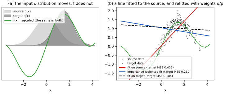
(b) Unbiased, with variance. \(\hat R_w=\frac1N\sum_nw_n\ell_n\) is unbiased for \(R(f,q)\), and its variance is \(\frac1N\big(\E_p[w^2\ell^2]-R^2\big)\), finite iff \(\E_p[w^2\ell^2]<\infty\). For Gaussians \(p=\N(m_p,s_p^2)\), \(q=\N(m_q,s_q^2)\) and \(\ell\equiv1\), completing the square gives \[ \E_p[w^2]=\frac{s_p}{s_q^2\sqrt{2\pi}}\sqrt{\frac{\pi}{A}}\,\exp\!\Big(\frac{B^2}{A}-\frac{m_q^2}{s_q^2}+\frac{m_p^2}{2s_p^2}\Big),\quad A=\frac{2s_p^2-s_q^2}{2s_p^2s_q^2},\ B=\frac{m_q}{s_q^2}-\frac{m_p}{2s_p^2}, \] which is finite iff \(s_q^2<2s_p^2\) (for \(A>0\)). A target that is wider than \(\sqrt2\) times the source has infinite weight variance however many points are used. The relevant measure of reliability is the effective sample size \(\mathrm{ESS}=(\sum_nw_n)^2/\sum_nw_n^2\approx N/\E_p[w^2]\) (gap 11.8). For the setting of Figure 19.10, \(p=\N(0,1)\) and \(q=\N(1.5,0.8^2)\), \(\E_p[w^2]=5.61\) and \(\mathrm{ESS}/N=17.8\%\); a simulation with three million draws gives \(17.9\%\).
(c) Why a conditional model can still be hurt. Fit \(f_\beta(x)=\beta^\T\varphi(x)\) by least squares. The population minimiser under input law \(p\) is \(\beta_p=\big(\E_p[\varphi\varphi^\T]\big)^{-1}\E_p[\varphi\,y]\). If the model is well specified, \(\E[y\given x]=\beta_\star^\T\varphi(x)\), then \(\E_p[\varphi y]=\E_p[\varphi\varphi^\T]\beta_\star\) and \(\beta_p=\beta_\star\) for every \(p\) with a nonsingular design: the shift is harmless. If it is misspecified, \(\beta_p\) depends on \(p\) and differs from \(\beta_q\): the model spends its capacity where \(p\) puts mass. With weights \(w=q/p\), the weighted normal equations have matrices \(\E_p[w\varphi\varphi^\T]=\E_q[\varphi\varphi^\T]\) and \(\E_p[w\varphi y]=\E_q[\varphi y]\), so the weighted population solution is exactly \(\beta_q\), the best fit for the target. In the book's picture (Figure 19.10), a line fitted to a wiggly function over the source region is a poor line over the target region.
(d) Numbers for Figure 19.10. Take \(f(x)=\sin(1.2x)+0.25x\), source \(\N(0,1)\), target \(\N(1.5,0.8^2)\), a straight-line model. The population source line is \(0.834\,x\) (intercept 0), with target mean squared error \(0.609\) about \(f\); the best line for the target is \(0.872+0.078x\) with error \(0.175\), which importance weighting reaches in the population. When the truth is itself a line (\(f=0.8x\)) the source and target lines coincide (both \(0.8x\)) and the shift costs nothing, as in (c). Bias against variance. Weighting removes a bias at the price of variance (the ESS above): with 120 source points the weighted fit has target error 0.210 in Figure 19.10 against 0.184 for an oracle fitted to target data and 0.422 for the unweighted fit, but for a small \(N\) or a larger shift the weights can be so unbalanced that the unweighted fit wins, and when the model is well specified plain least squares is more efficient (Shimodaira, 2000).
See also: gap 11.8 (self-normalised importance sampling); All of Statistics, 24.3 importance sampling.
19.5.2.1 Why is covariate shift a problem for discriminative models?
p. 748 If \(p(y\given x)\) is right everywhere, a shift of \(p(x)\) changes nothing. But a model is typically accurate only in parts of the input space: Figure 19.10b shows a line fitted over the whole source support doing badly on the target, while the same line fitted to the part of the space where the target has mass does well (gap 19.7(c)). Move the target in the demo to see it: covariate shift and importance weights, preset 2 is this figure; preset 3 has a well-specified model and no harm from the shift.
19.5.2.2 How should we estimate the ERM weights?
pp. 748–749 One could fit density models to the source and the target, but density estimation is hard in high dimension. It is easier to estimate the ratio directly with a binary classifier (Section 2.7.5). With equal numbers of source and target samples labelled \(c=-1\) and \(c=1\), \[ p(c=1\given x)=\frac{q(x)}{q(x)+p(x)},\tag{19.17} \] so \(\dfrac{p(c=1\given x)}{p(c=-1\given x)}=\dfrac{q(x)}{p(x)}\), and if the classifier is \(f(x)=\sigma(h(x))\) the weights are \[ w_n=\frac{1/(1+e^{-h(x_n)})}{e^{-h(x_n)}/(1+e^{-h(x_n)})}=e^{h(x_n)}.\tag{19.18} \] This requires \(q(x)>0\Rightarrow p(x)>0\), and gives no guarantee beyond the source support.
Filling the gap 19.8: the density ratio from a classifier, unequal sample sizes, and a worked case pp. 748–749
Derivation
Why the classifier's odds are the ratio. Pool the two samples, with \(N_p\) source and \(N_q\) target points, and let \(c\) be the domain indicator. The pooled density of \(x\) is a mixture with weights \(N_p/N\) and \(N_q/N\), so by Bayes' rule \(P(c=1\given x)=\dfrac{N_q\,q(x)}{N_q\,q(x)+N_p\,p(x)}\), and the odds are \(\dfrac{N_q}{N_p}\dfrac{q(x)}{p(x)}\). With \(h\) the log-odds, \[ w(x)=\frac{q(x)}{p(x)}=\frac{N_p}{N_q}\,e^{h(x)}\ ,\] which is (19.18) when \(N_p=N_q\); with unbalanced samples the factor \(N_p/N_q\) must not be forgotten (without it the weights have the wrong mean; since \(\E_p[w]=1\), the factor can also be restored by normalising the weights to average one).
Why logistic regression estimates \(h\). The logistic loss is a proper scoring rule: its population minimiser over all functions is the true log-odds \(h^\star(x)=\log\frac{P(c=1\given x)}{P(c=0\given x)}\) (set the derivative of \(\E[\ell]\) in \(h(x)\) to zero pointwise: \(\sigma(h)=P(c=1\given x)\)). Over a restricted family the result is the best approximation in that family, and it is exact if the family contains \(h^\star\). Gaussian example. For \(p=\N(m_p,s^2)\) and \(q=\N(m_q,s^2)\), \(\log\frac{q}{p}=\frac{(m_q-m_p)x}{s^2}-\frac{m_q^2-m_p^2}{2s^2}\) is linear in \(x\), so linear logistic regression (features \(1,x\)) is well specified; for different variances \(\log(q/p)\) is quadratic and the features \(1,x,x^2\) are needed. I confirm numerically for \(m_p=0\), \(m_q=1.2\), \(s=1\): balanced logistic regression returns intercept \(-0.714\) and slope \(1.196\) against the exact \(-0.72\) and \(1.2\), and with \(N_p=3N_q\) the weights \(\frac{N_p}{N_q}e^{h}\) match \(q/p\) to within 1.2% over \([-2,3]\).
Cautions. (i) A classifier trained to near-perfect separation (high dimension, small samples) has large \(|h|\) and enormous weights: regularise it or clip. (ii) Fitting the classifier and then weighting the same source points that trained it makes the weights slightly overfit; cross-fitting avoids this. (iii) Only calibrated probabilities give the right ratio; an overconfident network gives the right ordering but the wrong scale. (iv) My implementation (density_ratio_logistic) uses Newton's method on the logistic loss and agrees with scikit-learn's solver to \(2\times10^{-3}\).
See also: 2.7.5 density ratio estimation by a classifier.
19.5.3 Unsupervised domain adaptation for covariate shift
pp. 749–750 Unsupervised domain adaptation (UDA) assumes labelled source data \(\D_1=\D^s_L\sim p(x,y)\) and unlabelled target data \(\D_2=\D^t_U\sim q(x)\), and uses the target inputs to make the predictor invariant, instead of reweighting. The book describes domain-adversarial learning (Ganin et al., 2016). A feature extractor \(f_\alpha\) maps either domain to features, a domain classifier \(c_\beta\) predicts which domain a feature came from, and a label classifier \(g_\gamma\) predicts \(y\). The extractor is trained so that the domain cannot be told from its output, leaving only features common to both domains: \[ \min_\gamma\max_{\alpha,\beta}\ \frac1{N_1+N_2}\sum_{x_n\in\D_1,\D_2}\ell\big(d_n,c_\beta(f_\alpha(x_n))\big)+\frac1{N_1}\sum_{(x_n,y_n)\in\D_1}\ell\big(y_n,g_\gamma(f_\alpha(x_n))\big).\tag{19.19} \] The objective is implemented with a gradient-reversal layer and is related to GANs (Section 26.7.6). (A remark on the printed form of (19.19) is in Notes on the book, item 2.)
Filling the gap 19.9: why domain-adversarial training works, and what gradient reversal does pp. 749–750
Derivation
(a) A bound that explains the objective. Let \(h\) range over a hypothesis class \(\mathcal H\) of binary classifiers, \(f_S,f_T\) be the labelling functions of the two domains and \(\varepsilon_D(h,h')=P_{x\sim D}[h(x)\ne h'(x)]\), \(\varepsilon_D(h)=\varepsilon_D(h,f_D)\). Define \(d=\sup_{h,h'\in\mathcal H}|\varepsilon_S(h,h')-\varepsilon_T(h,h')|\) (the discrepancy of the two input laws as seen by \(\mathcal H\)) and \(\lambda=\min_{h}\,[\varepsilon_S(h)+\varepsilon_T(h)]=\varepsilon_S(h^\ast)+\varepsilon_T(h^\ast)\) (the error of the best joint hypothesis). Claim: for every \(h\in\mathcal H\), \[ \varepsilon_T(h)\le\varepsilon_S(h)+d+\lambda. \] Proof. The disagreement \(\varepsilon_D(\cdot,\cdot)\) is a pseudo-metric (it is the probability of a symmetric difference), so it satisfies the triangle inequality. Then \(\varepsilon_T(h)\le\varepsilon_T(h^\ast)+\varepsilon_T(h,h^\ast)\le\varepsilon_T(h^\ast)+\varepsilon_S(h,h^\ast)+d\le\varepsilon_T(h^\ast)+\varepsilon_S(h)+\varepsilon_S(h^\ast)+d=\varepsilon_S(h)+\lambda+d\). \(\square\) (Ben-David et al., 2010, with their divergence \(d_{\mathcal H\Delta\mathcal H}\) equal to \(2\sup_A|P_S(A)-P_T(A)|\) over the sets \(A\) where two hypotheses disagree; my \(d\) is one convenient form of it. I confirm the inequality for every hypothesis on 200 random finite domains.) So target error is controlled by source error, the input discrepancy and the joint error \(\lambda\); the third is unobservable without target labels, the second is the quantity that adversarial training reduces, and if \(\lambda\) is large no feature alignment can help.
(b) The domain-classifier loss measures the discrepancy. Let the two domains have equal weight and let \(P,Q\) be the feature laws of the source and the target. The cross-entropy of the best domain classifier \(c^\ast(z)=P(d=1\given z)=\frac{q(z)}{p(z)+q(z)}\) is the conditional entropy \(H(d\given z)=H(d)-I(d;z)=\log2-\JS(P,Q)\), because with balanced domains the mutual information between the domain and the feature is the Jensen-Shannon divergence \(\JS(P,Q)=\frac12\KL(P\|M)+\frac12\KL(Q\|M)\), \(M=\frac12(P+Q)\). (A quadrature for \(P=\N(0,1)\), \(Q=\N(1.5,1)\) confirms the identity.) So, with the discriminator \(\beta\) at its optimum, maximising the domain loss over the extractor \(\alpha\) is minimising \(\JS(P_\alpha,Q_\alpha)\): the extractor is pushed to make the two feature distributions indistinguishable.
(c) Gradient reversal. Insert a layer \(\mathcal R\) between the extractor and the domain classifier with \(\mathcal R(z)=z\) in the forward pass and \(\partial\mathcal R/\partial z=-\lambda I\) in the backward pass. Ordinary stochastic gradient descent on the sum of the label loss \(L_y\) and the domain loss \(L_d\) of the composite network then updates \(\beta\leftarrow\beta-\eta\,\partial L_d/\partial\beta\) (a better discriminator), \(\gamma\leftarrow\gamma-\eta\,\partial L_y/\partial\gamma\), and \(\alpha\leftarrow\alpha-\eta\big(\partial L_y/\partial\alpha-\lambda\,\partial L_d/\partial\alpha\big)\): descent on the label loss and ascent on the domain loss for the extractor. These are the gradient steps of the saddle-point problem \(\min_{\alpha,\gamma}\max_\beta\,[L_y-\lambda L_d]\) without a second optimiser, and as for GANs, convergence is not guaranteed and training can oscillate.
See also: Introduction volume, 19.2.5 domain adaptation.
19.5.4 Unsupervised techniques for label shift
p. 750 Blackbox shift estimation (Lipton, Wang and Smola, 2018) tackles label shift without target labels. Assume \(q(x,y)=p(x\given y)q(y)\). For any deterministic predictor \(f\) with \(\hat y=f(x)\), \[ p(x\given y)=q(x\given y)\ \Longrightarrow\ p(f(x)\given y)=q(f(x)\given y)\ \Longrightarrow\ p(\hat y\given y)=q(\hat y\given y).\tag{19.20} \] Let \(\mu_i=q(\hat y=i)\) be the fraction of target inputs predicted as class \(i\), \(q(y=j)\) the unknown target prior, and \(C_{ij}=p(\hat y=i\given y=j)\) the confusion matrix estimated on the source. Then \[ \mu_{\hat y}=\sum_yq(\hat y\given y)q(y)=\sum_yp(\hat y\given y)q(y)=\sum_y\frac{p(\hat y,y)}{p(y)}q(y),\tag{19.21} \] \[ \mu_i=\sum_jC_{ij}q_j\quad\Longrightarrow\quad\mu=Cq\quad\Longrightarrow\quad q=C^{-1}\mu,\tag{19.22} \] provided \(C\) is invertible and every label with \(q(y)>0\) has \(p(y)>0\). With \(q\) known, the classifier is corrected for the new prior: \[ q(y\given x)=\frac{q(x\given y)q(y)}{q(x)}=\frac{p(x\given y)q(y)}{q(x)}=\frac{p(y\given x)p(x)}{p(y)}\frac{q(y)}{q(x)}=p(y\given x)\,\frac{q(y)}{p(y)}\,\frac{p(x)}{q(x)},\tag{19.23} \] where \(p(x)/q(x)\) does not depend on \(y\) and is removed by normalising over \(y\). The method needs (1) an invertible \(C\), (2) no new labels at test time, (3) that only the label prior moves. Garg et al. (2020) estimate \(q(y)\) by maximum likelihood instead of moment matching.
Filling the gap 19.10: why \(q=C^{-1}\mu\), when \(C\) is invertible, the error of the estimate, and the EM alternative pp. 750–751
Derivation
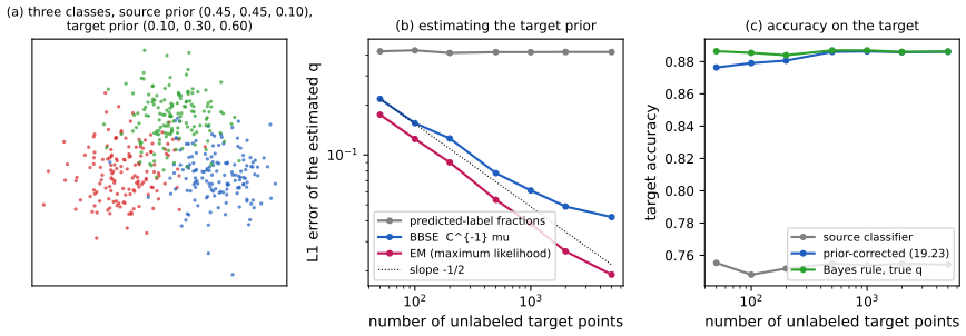
(a) The moment equation. The predictor \(\hat y=f(x)\) is a function of \(x\) alone, so \(P(\hat y=i\given y=j)=\int\ind(f(x)=i)\,p(x\given y=j)\,\d x\), a functional of \(p(x\given y)\) only; under label shift the class-conditional is the same under \(q\), which is (19.20). Then \(\mu_i=q(\hat y=i)=\sum_jq(\hat y=i\given y=j)q(y=j)=\sum_jC_{ij}q_j\) by the law of total probability, which is (19.22) (the book's sum index in (19.22) should be \(j\); Notes on the book, item 3). I confirm with a three-class Gaussian world: the predicted-label fractions on 400,000 target points match \(Cq\) to within 0.004.
(b) When is \(C\) invertible? The columns of \(C\) sum to one, \(\sum_iC_{ij}=1\). If each class is classified correctly more than half the time, \(C_{jj}>\frac12\) for all \(j\), then \(\sum_{i\ne j}|C_{ij}|=1-C_{jj}<C_{jj}\): \(C\) is strictly diagonally dominant by columns, hence invertible (Levy-Desplanques). The book's wording "the model predicts class \(y_j\) correctly more often than any other class" (each \(C_{jj}\) larger than the other entries of its column) is not sufficient: \(C=\begin{pmatrix}0.43&0.293&0.156\\0.415&0.396&0.377\\0.155&0.311&0.467\end{pmatrix}\) has its largest entry on the diagonal of every column and its third column equals twice the second minus the first, so \(\det C=0\) and different priors \(q\) give the same \(\mu\) (not identifiable). Also a necessary condition: if two classes are predicted with the same distribution (equal columns) the problem is not identifiable. The condition number of \(C\) controls how much sampling noise is amplified.
(c) Error with a known \(C\). Let \(\hat\mu\) be the predicted-class fractions of \(n\) target points. The counts are multinomial\((n,\mu)\), so \(\E\hat\mu=\mu\) and \(\cov\hat\mu=\frac1n(\diag\mu-\mu\mu^\T)\). Hence \(\hat q=C^{-1}\hat\mu\) is unbiased with \[ \cov\hat q=\frac1n\,C^{-1}\big(\diag\mu-\mu\mu^\T\big)C^{-\T}, \] so the error shrinks like \(1/\sqrt n\) (my simulation of 60,000 replications with \(n=1500\) reproduces the standard deviations 0.0121, 0.0156, 0.0182). If \(\hat C\) is estimated on \(n_s\) held-out source points, \(\hat q-q\approx C^{-1}(\hat\mu-\mu)-C^{-1}(\hat C-C)q\): the second term does not shrink as the number of target points grows, only with \(n_s\), and is larger for a rare class (its column of \(C\) rests on few examples). That is the error floor in Figure 19.28b. In practice \(\hat q\) can have negative entries; project onto the simplex (clip and renormalise).
(d) The prior correction (19.23). Only the last identity needs a word: \(q(y\given x)\propto p(y\given x)q(y)/p(y)\) in \(y\) for fixed \(x\), and the normalising constant is fixed by \(\sum_yq(y\given x)=1\). This is the Bayes-optimal classifier for the target prior, as a logit shift: add \(\log q_y-\log p_y\) to the log-probability of class \(y\). It is only as good as the calibration of \(p(y\given x)\); I verify the identity against the exact posteriors in a Gaussian mixture.
(e) EM as the likelihood alternative. Under the label-shift assumption the target density of an input is \(q(x)=\sum_yq(y)p(x\given y)=p(x)\sum_y\frac{q(y)}{p(y)}p(y\given x)\), so with source posteriors \(p(y\given x_n)\) the target log-likelihood in \(q\) is, up to a constant, \(\sum_n\log\sum_y\frac{q_y}{p_y}p(y\given x_n)\), concave in \(q\). The EM iteration \(q_y\leftarrow\frac1n\sum_n\frac{(q_y/p_y)\,p(y\given x_n)}{\sum_{y'}(q_{y'}/p_{y'})\,p(y'\given x_n)}\) (Saerens, Latinne and Decaestecker, 2002) increases it at every step and needs no inverse, but uses probabilities rather than hard labels and so needs a calibrated classifier. In Figure 19.28b it is more accurate than blackbox shift estimation at every sample size.
See also: demo label shift and blackbox estimation.
19.5.5 Test-time adaptation
pp. 750–751 In test-time adaptation (TTA) the parameters are updated continuously while the model is deployed; unlike unsupervised domain adaptation, only the model trained on the source is kept, not the source data. Test-time training (TTT; Sun et al., 2020) trains a Y-shaped network with a shared feature layer \(h\), a label head and a self-supervised head (for instance predicting the rotation angle of the input), and at test time updates the shared features by the self-supervised loss, which needs no label. If no such proxy exists, TENT (Wang et al., 2021) updates the classifier to minimise the entropy of its predictions on a batch of test examples (Goyal et al., 2022, justify it from a meta-learning view; BACS is a Bayesian version, Zhou and Levine, 2021). MEMO (Zhang, Levine and Finn, 2022) works for any architecture: augment the single test input \(x\) into \(\tilde x_1,\dots,\tilde x_B\) and minimise the entropy of the averaged prediction \[ p(y\given x,w)=\frac1B\sum_{b=1}^Bp(y\given\tilde x_b,w),\tag{19.24} \] which makes the predictions agree across perturbations and be confident. The alternative is pseudo-labelling: label the target data with the source model and self-train, with regularisers against overfitting the mistakes.
Filling the gap 19.11: what entropy minimisation optimises pp. 750–751
Derivation
(a) The TENT gradient. For softmax probabilities \(p=\softmax(z)\) and entropy \(H(p)=-\sum_kp_k\log p_k\), \(\partial p_k/\partial z_j=p_k(\delta_{kj}-p_j)\), and \[ \frac{\partial H}{\partial z_j}=-\sum_k\frac{\partial p_k}{\partial z_j}(\log p_k+1)=-p_j\big(\log p_j+H(p)\big) \] (using \(\sum_k\partial p_k/\partial z_j=0\)). The logit of a class whose log probability is above \(-H\) (above the average) is pushed up, the others down: gradient descent on the entropy makes the currently most probable class more probable. The minimum \(H=0\) is a one-hot distribution, so entropy minimisation is a form of self-training and inherits its failure mode: a wrong but confident prediction is reinforced. (The uniform distribution is a stationary point, but the maximum, not a minimum.) I check the gradient formula by finite differences.
(b) MEMO's marginal entropy. Let \(p_b=p(\cdot\given\tilde x_b,w)\) and \(\bar p=\frac1B\sum_bp_b\) as in (19.24). Then \[ H(\bar p)=\frac1B\sum_bH(p_b)+\frac1B\sum_b\KL(p_b\,\|\,\bar p). \] Proof. \(\frac1B\sum_b\KL(p_b\|\bar p)=\frac1B\sum_b\sum_yp_b(y)\log p_b(y)-\sum_y\bar p(y)\log\bar p(y)=-\frac1B\sum_bH(p_b)+H(\bar p)\). \(\square\) Since \(\KL\ge0\), \(H(\bar p)\ge\frac1B\sum_bH(p_b)\) (concavity of entropy), and minimising the marginal entropy minimises two things at once: the average entropy of the individual predictions (confidence) and the average divergence of each prediction from the consensus (consistency across augmentations, a generalised Jensen-Shannon divergence). This is the sense of "gives the same prediction for each perturbation and confident": the term that is absent from the entropy of a single prediction is the disagreement among the augmented views. A numerical experiment with random distributions confirms the identity to \(10^{-10}\).
19.6 Learning from multiple distributions
p. 751 The setting of 19.2 has one source and one target. Now the model is trained on \(J\ge2\) distributions (Figure 19.11, a schematic of the problem set-ups and the families of solutions, is not reproduced): transfer learning if there are two, with labelled target data; multitask learning if all \(J\) are of interest; domain generalisation if the target is unseen and unlabelled; continual learning (19.7) if the distributions arrive in a stream.
19.6.1 Multitask learning
pp. 751–752 In multitask learning (MTL; Caruana, 1997) there are labelled data \(\D_j=\{(x_n^j,y_n^j)\}_{n\le N_j}\) from \(J\) distributions and the goal is one model \(f(x,j)\in\mathcal Y_j\) that predicts all of them, for instance a per-pixel semantic label (\(\mathcal Y_1=\{1,\dots,C\}^{HW}\)) and a per-pixel depth (\(\mathcal Y_2=\R^{HW}\)) from one image. By empirical risk minimisation over all tasks, \[ f^\ast=\argmin_f\sum_{j=1}^J\sum_{n=1}^{N_j}\ell_j\big(y_n^j,f(x_n^j,j)\big),\tag{19.25} \] with a suitably scaled loss \(\ell_j\) per task. The simplest architecture shares a trunk and has one output head per task (Figure 19.12, a diagram), which often does worse than separate networks; cross-stitch networks (Misra et al., 2016) learn a weighted combination of the activations of single-task networks (Zhang and Yang, 2021, review neural approaches). MTL does not always help: task interference or negative transfer can hurt, and then separate networks are better.
19.6.2 Domain generalization
pp. 752–754 In domain generalisation (DG) the model is trained on \(J\) labelled source environments (domains), each possibly with meta-data such as time, place or device, and tested on a new target \(t=J+1\) with no target labels. Unlike MTL, only target accuracy matters, so some assumption must tie \(p_t(x,y)\) to the \(p_j\). One is the hierarchical Bayesian model of Figure 19.13: \(p_t(x,y)=p(x\given\phi_t)p(y\given x,w_t)\) with \(w_t\) drawn from a population-level \(w_0\) shared with the other environments (and likewise for \(\phi\), which a discriminative model need not learn; Baxter, 2000). For a Gaussian linear model this is the model of gap 19.6: environment parameters \(w_j\sim\N(w_0,\tau^2I)\) shrink towards the common \(w_0\), and for the unseen target the predictive variance is \(\sigma^2+\tau^2\|\varphi(x)\|^2\), where the second term, the environment-to-environment variability, does not vanish with more data from the \(J\) environments. Many DG methods exist; Gulrajani and Lopez-Paz (2021) found none consistently better than ERM on the pooled data (Section 15.5 and 17.6 cover hierarchical GLMs and MLPs).
19.6.3 Invariant risk minimization
pp. 754–755 Invariant risk minimisation (IRM; Arjovsky et al., 2019) aims at a predictor that works across all environments and does not lean on spurious features. It extends invariant causal prediction (ICP; Peters, Buehlmann and Meinshausen, 2016), which tests which sets of variables are direct causes of the outcome in every environment (Figure 19.14, a diagram). IRM handles high-dimensional inputs (pixels) by asking for a predictor that does well on average and is simultaneously optimal in every environment: \[ f^\ast=\argmin_{f\in\mathcal F}\sum_{j=1}^J\frac1{N_j}\sum_{n=1}^{N_j}\ell\big(y_n^j,f(x_n^j)\big)\tag{19.26} \] \[ \text{such that}\quad f\in\argmin_{g\in\mathcal F}\frac1{N_j}\sum_{n=1}^{N_j}\ell\big(y_n^j,g(x_n^j)\big)\ \text{ for all } j\in\mathcal E.\tag{19.27} \] The intuition: many functions fit a single environment, but one that is optimal in every environment is more likely to use causal than spurious features. Later work shows the principle often fails for covariate shift, in theory (Rosenfeld, Ravikumar and Risteski, 2021) and in practice (Gulrajani and Lopez-Paz, 2021), though it can work for anticausal models (Ahuja et al., 2021). The bilevel problem is replaced in practice by a penalty (IRMv1): the squared gradient of each environment's risk with respect to a scalar multiplier of the representation, evaluated at one.
Filling the gap 19.12: IRM on an exactly solvable spurious-feature model pp. 754–755
Derivation
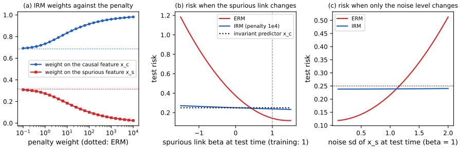
The model (my own). Environment \(e\) has a causal feature \(x_c\sim\N(0,1)\), a label \(y=x_c+\varepsilon_y\), \(\varepsilon_y\sim\N(0,s_y^2)\), and a spurious feature that is a child of the label, \(x_s=\beta y+\varepsilon_e\), \(\varepsilon_e\sim\N(0,s_e^2)\) (anticausal). The regression of \(y\) on \(x_c\) alone has the same coefficient 1 and risk \(s_y^2\) in every environment; the regression on both features uses \(x_s\) with an environment-dependent weight. Write \(x=(x_c,x_s)\), \(\Sigma_e=\E^e[xx^\T]\), \(c_e=\E^e[xy]\) and \(v=\E[y^2]=1+s_y^2\); then \[ \Sigma_e=\begin{pmatrix}1&\beta\\\beta&\beta^2v+s_e^2\end{pmatrix},\qquad c_e=\begin{pmatrix}1\\\beta v\end{pmatrix},\qquad R^e(\theta)=\theta^\T\Sigma_e\theta-2\theta^\T c_e+v \] for the predictor \(\theta^\T x\). Single environment. For \(\beta=1\) the optimal weights \(\Sigma_e^{-1}c_e\) are \(\big(\frac1{s_y^2},\frac1{s_e^2}\big)/\Lambda\) with \(\Lambda=\frac1{s_y^2}+\frac1{s_e^2}\) (Gaussian conditioning of \(y\) on its two noisy measurements, \(x_c\) with variance \(s_y^2\) and \(x_s\) with variance \(s_e^2\)): the weight on the spurious feature is larger when \(x_s\) is cleaner. ERM on two training environments with \(\beta=1\), \(s_e\in\{0.3,1.0\}\), \(s_y=0.5\) minimises the average risk, so \(\theta_{\mathrm{ERM}}=\big(\tfrac12(\Sigma_1+\Sigma_2)\big)^{-1}\tfrac12(c_1+c_2)=(0.686,0.314)\): a third of the weight is on the spurious feature.
The invariance condition. Let \(\Phi(x)=\theta^\T x\) be the representation and \(w\) a scalar head. In environment \(e\), \(R^e(w\Phi)\) is a convex quadratic in \(w\), so \(w=1\) is optimal for that environment iff \(\frac{\d}{\d w}R^e(w\Phi)\big|_{w=1}=2\big(\theta^\T\Sigma_e\theta-\theta^\T c_e\big)=0\). This is the constraint (19.27) for the scalar head (first-order, and sufficient by convexity), and the IRMv1 penalty is the sum over environments of its square. Theorem (identification). If two training environments have \(\beta=1\) and \(s_{e}\)'s that differ, the only non-zero representation satisfying the constraint in both is \(\theta=(1,0)\), the causal predictor. Proof. With \(\theta=(a,b)\) and \(\beta=1\), \(\theta^\T\Sigma_e\theta-\theta^\T c_e=\big[a^2+2ab+b^2v-a-bv\big]+b^2s_e^2\); the bracket does not depend on \(e\). Setting this to zero in both environments and subtracting gives \(b^2(s_1^2-s_2^2)=0\), so \(b=0\), and then \(a^2-a=0\), so \(a=1\) (or \(a=0\)). \(\square\) If \(s_1=s_2\) the two environments are indistinguishable and the constraint does not single out \(\theta=(1,0)\): environment diversity is what identifies the invariant feature.
Numbers (Figure 19.29). The invariant predictor has risk \(0.25\) in every environment and every test link \(\beta\). ERM has training risks \(0.126\) and \(0.216\), better than the invariant predictor, because it uses \(x_s\); but when the link flips to \(\beta=-1\) its risk is \(0.852\), and when only the noise level of \(x_s\) rises to \(s_e=2\) it is \(0.513\). Minimising the risk plus \(10^4\) times the penalty gives \((0.981,0.024)\) with risks \(0.238\) in both training environments and \(0.264\) after the flip; the weight on \(x_s\) tends to zero as the penalty grows (\(0.011\) at \(10^5\)). The cost of invariance in this toy is the extra risk at \(\beta=1\) (\(0.25\) against \(0.14\)), the price of insuring against a link that may change. The example is anticausal (the label causes the spurious feature), in line with the book's remark that IRM can work there.
19.6.4 Meta learning
p. 755 The goal of meta-learning is to "learn the learning algorithm" (Thrun and Pratt, 1998). The meta-learner is given datasets from several distributions, as in domain generalisation, except that each distribution is split into a training and a test part, so that it can practise generalising from a training set to a test set (Hospedales et al. 2020 review). The book follows the hierarchical Bayesian framework of Gordon et al. (2019).
19.6.4.1 Meta-learning as probabilistic inference for prediction
pp. 755–757 There are \(J\) tasks, each with a training set \(\D^j_{\mathrm{train}}=\{(x_n^j,y_n^j)\}_{n\le N^j}\) and a test set \(\D^j_{\mathrm{test}}=\{(\tilde x_m^j,\tilde y_m^j)\}_{m\le M^j}\), task-specific parameters \(w_j\) and shared parameters \(w_0\) (Figure 19.15). A point estimate is learned for \(w_0\) (shared, little uncertainty) and an approximate posterior \(p(w_j\given\D^j_{\mathrm{train}},w_0)\) for \(w_j\) (little data per task), giving the posterior predictive \[ p(\tilde y^j\given\tilde x^j,\D^j_{\mathrm{train}},w_0)=\int p(\tilde y^j\given\tilde x^j,w_j)\,p(w_j\given\D^j_{\mathrm{train}},w_0)\,\d w_j.\tag{19.28} \] Because the exact posterior is intractable, an amortised approximation \(q_\phi(\tilde y^j\given\tilde x^j,\D^j_{\mathrm{train}},w_0)\) is learned (10.1.5) by making it as close as possible to the true predictive: \[ \phi^\ast=\argmin_\phi\E_{p(\D_{\mathrm{train}},\tilde x)}\Big[\KL\big(p(\tilde y\given\tilde x,\D_{\mathrm{train}},w_0)\,\big\|\,q_\phi(\tilde y\given\tilde x,\D_{\mathrm{train}},w_0)\big)\Big]\tag{19.29} \] \[ =\argmax_\phi\E_{p(\D_{\mathrm{train}},\tilde x)}\Big[\E_{p(\tilde y\given\tilde x,\D_{\mathrm{train}},w_0)}\big[\log q_\phi(\tilde y\given\tilde x,\D_{\mathrm{train}},w_0)\big]\Big]\tag{19.30} \] \[ =\argmax_\phi\E_{p(\D_{\mathrm{train}},\tilde x,\tilde y)}\Big[\log\int p(\tilde y\given\tilde x,w)\,q_\phi(w\given\D_{\mathrm{train}},w_0)\,\d w\Big],\tag{19.31} \] using \(p(\tilde y\given\tilde x,\D_{\mathrm{train}},w_0)\approx p(\tilde y\given\tilde x,\D_{\mathrm{train}})\). A Monte Carlo estimate over \(J\) sampled tasks and \(S\) draws \(w^j_s\sim q_\phi(w^j\given\D^j,w_0)\) is, with \(M\) test points per task, \[ \mathcal L_{\mathrm{meta}}(w_0,\phi)=\frac1{MJ}\sum_{m=1}^M\sum_{j=1}^J\log\Big(\frac1S\sum_{s=1}^Sp\big(\tilde y^j_m\given\tilde x^j_m,w^j_s\big)\Big).\tag{19.32} \] This differs from the standard amortised variational objective, which fits the expected log likelihood of all data of a task (train and test pooled) minus a KL penalty, \[ \mathcal L_{\mathrm{VI}}(w_0,\phi)=\frac1J\sum_j\Big[\sum_{(x,y)\in\D^j_{\mathrm{all}}}\frac1S\sum_s\log p(y\given x,w^j_s)-\KL\big(q_\phi(w^j\given\D^j_{\mathrm{all}},w_0)\,\|\,p(w^j\given w_0)\big)\Big],\tag{19.33} \] in three ways: the meta objective takes the log of an average where the standard one takes the average of a log (the former can be provably better for predictive accuracy, as Morningstar, Alemi and Dillon, 2020, point out), it fits the forward KL rather than the reverse KL, and it has no KL penalty on the task posterior.
Filling the gap 19.13: from the KL to the meta-learning objective, and log-of-average against average-of-log pp. 755–757
Derivation
(19.29)→(19.30). For fixed \((\D_{\mathrm{train}},\tilde x)\), \(\KL(p\|q_\phi)=\E_p[\log p]-\E_p[\log q_\phi]\) and the first term does not involve \(\phi\), so minimising the KL maximises \(\E_p[\log q_\phi]\). (The book prints \(\argmin\) in front of (19.30) and (19.31); it should be \(\argmax\), or the expressions should carry a minus sign: Notes on the book, item 4. The Monte Carlo objective (19.32) is correctly a quantity to maximise.)
(19.30)→(19.31). The outer expectation over \((\D_{\mathrm{train}},\tilde x)\) and the inner one over \(\tilde y\) from the predictive combine into one expectation over the joint \(p(\D_{\mathrm{train}},\tilde x,\tilde y)\) (law of total expectation, with \(\tilde y\) drawn from the very model that generated the data); and \(q_\phi(\tilde y\given\tilde x,\D_{\mathrm{train}},w_0)\) is by definition the predictive built from \(q_\phi(w\given\D_{\mathrm{train}},w_0)\), \(\int p(\tilde y\given\tilde x,w)q_\phi(w\given\D_{\mathrm{train}},w_0)\,\d w\). Replacing the outer expectation over tasks by an average over \(J\) sampled tasks (each split into train and test) and the integral by \(S\) draws gives (19.32).
Log of the average against average of the log. For positive numbers \(a_1,\dots,a_S\), Jensen's inequality for the concave logarithm gives \(\log\big(\frac1S\sum_sa_s\big)\ge\frac1S\sum_s\log a_s\). With \(a_s=p(\tilde y\given\tilde x,w_s)\) the summand of (19.32) is therefore at least the average of log likelihoods that appears in (19.33), term by term, and strictly greater unless the \(a_s\) agree; the gap is the amount by which sampling the task parameter and averaging the predictions beats evaluating each sampled model on its own, and the gap grows with the disagreement among the \(w_s\). (I confirm the inequality on random likelihoods.) Moreover the expectation of the log of an \(S\)-sample average is non-decreasing in \(S\) and tends to the log of the exact predictive, the same fact that makes importance-weighted bounds tighter with more samples (Domke and Sheldon, 2018); the finite-\(S\) estimator (19.32) is a lower bound on the log predictive probability in expectation, so maximising it is safe.
The point-estimate case (neural processes). If \(q_\phi(w_j\given\D^j,w_0)=\delta\big(w_j-A_\phi(\D^j,w_0)\big)\), the integral in (19.28) collapses by the sifting property: \(q(\tilde y^j\given\tilde x^j,\D^j,w_0)=p\big(\tilde y^j\given\tilde x^j,A_\phi(\D^j,w_0),w_0\big)\) (19.34). It can be evaluated and maximised by ordinary supervised maximum likelihood over \((\phi,w_0)\), which is a neural process (Garnelo et al., 2018). MAML takes \(A(\D^j,w_0)=w_0+\eta\nabla_w\sum_n\log p(y_n^j\given x_n^j,w)\big|_{w_0}\) (19.35): one gradient step on the training log likelihood from the shared initialisation, and the meta-parameter \(w_0\) is trained by differentiating (19.34) through that step (Finn, Abbeel and Levine, 2017).
See also: Introduction volume, 19.5.1 MAML; 10.1.5 amortized inference.
19.6.4.2 Neural processes and 19.6.4.3 Gradient-based meta-learning (MAML)
p. 757 The two special cases (19.34) and (19.35) are derived in gap 19.13: a neural process uses a deterministic inference network \(A_\phi\) that maps a dataset to parameters, MAML uses one step of gradient ascent on the training log likelihood from \(w_0\).
19.6.4.4 Metric-based few-shot learning (prototypical networks)
pp. 757–758 Let \(w_0\) be the parameters of a shared feature extractor \(h_{w_0}(x)\) and the task-specific parameters the weights and biases of the last linear layer. Average the features of each class in a task's training set, \(\mu_c^j=\frac1{|\D_c^j|}\sum_{x\in\D_c^j}h_{w_0}(x)\) (19.36), and set the task parameters to the centroids and their squared norms, \[ \hat w_j=A(\D^j,w_0)=\Big[\mu_c^j,\,-\tfrac12\|\mu_c^j\|^2\Big]_{c=1}^C,\tag{19.37} \] \[ q(\tilde y^j=c\given\tilde x^j,\D^j,w_0)\propto\exp\big(-d(h_{w_0}(\tilde x),\mu_c^j)\big)=\exp\Big(h_{w_0}(\tilde x)^\T\mu_c^j-\tfrac12\|\mu_c^j\|^2\Big),\tag{19.38} \] with \(d\) the Euclidean distance (squared, with a factor \(\frac12\)): the prototypical network (Snell, Swersky and Zemel, 2017).
Filling the gap 19.14: a prototypical network is a Gaussian classifier with identity covariance pp. 757–758
Derivation
Expand \(\tfrac12\|h-\mu_c\|^2=\tfrac12\|h\|^2-h^\T\mu_c+\tfrac12\|\mu_c\|^2\). The first term is the same for every class, so it cancels in the softmax normalisation, leaving \(\exp\big(h^\T\mu_c-\tfrac12\|\mu_c\|^2\big)\propto\exp\big(-\tfrac12\|h-\mu_c\|^2\big)\): this is the second equality in (19.38) and shows that the classifier is a softmax regression with weight vector \(\mu_c\) and bias \(-\frac12\|\mu_c\|^2\), the parameters (19.37). Next, \(\N(h;\mu_c,I)=(2\pi)^{-D/2}\exp(-\frac12\|h-\mu_c\|^2)\) has the same normalising constant for every \(c\), so the posterior over classes under class-conditional densities \(\N(\mu_c,I)\) and equal priors is exactly (19.38). With class priors \(\pi_c\) the bias becomes \(-\frac12\|\mu_c\|^2+\log\pi_c\). A prototypical network is therefore the plug-in Bayes classifier of a Gaussian model with a shared identity covariance and means estimated from the few labelled examples of the task (linear discriminant analysis with \(\Sigma=I\)); episodic training of \(h_{w_0}\) makes the embedding such that this simple model is accurate. (I confirm numerically that the three forms agree.) Learning with a different covariance, or a different distance, changes the boundaries from hyperplanes to quadrics.
19.7 Continual learning
p. 758 In continual (or life-long) learning the system learns from a sequence of distributions \(p_1,p_2,\dots\). At step \(t\) it receives \[ \D_t=\{(x_n,y_n)\sim p_t(x,y):n=1{:}N_t\},\qquad p_t(x,y)=p_t(x)\,p(y\given f_t(x)),\tag{19.39} \] where \(f_t:\mathcal X_t\to\mathcal Y_t\) is an unknown prediction function (each distribution is a different task), and is evaluated on an independent test set \[ \D_t^{\mathrm{test}}=\{(x_n,y_n)\sim p^{\mathrm{test}}_t(x,y):n=1{:}N_t^{\mathrm{test}}\}.\tag{19.40} \] What the test set is made of defines the scenario. If it contains all tasks up to \(t\), the model must not forget (19.7.4). If it is only the current distribution, as in online learning (19.7.5), the model must adapt but need not remember. (Non-stationarity also occurs in reinforcement learning, through the changing policy and value function.)
19.7.1 Domain drift
pp. 758–759 Domain drift: \(p_t(x)\) changes (covariate shift over time) but \(f_t\) is constant; for example a self-driving car's vision system under changing light (Figure 19.16, a schematic). The test distribution is either the current input law \(p_t\) (the detector must work on dark images now) or the union \(\cup_{s\le t}p_s\) of everything seen so far (it must work on dark and light images).
19.7.2 Concept drift
pp. 759–760 Concept drift (Widmer and Kubat, 1996): \(p_t(x)\) is constant but \(f_t\) changes (Figure 19.17, a schematic); what counts as legal behaviour changes, or a sort-by-colour task is replaced by a sort-by-shape task. This is a stationary \(p(y\given x,\text{task})\) with an unobserved task, so the observed \(p(y\given x)\) changes. The prediction for one input \(x\) depends on when it is made, so the test distribution must move with time, or each input must be tagged with a time stamp or task identity.
19.7.3 Class incremental learning
pp. 760–761 In class incremental learning there is one fixed function \(f:\mathcal X\to\mathcal Y\) but at step \(t\) only a subset \(\mathcal Y_t\subset\mathcal Y\) of the classes is shown (for digits, \(\mathcal Y_1=\{0,1\}\), \(\mathcal Y_2=\{2,\dots,9\}\); Figure 19.18, a schematic). The scenarios (Figure 19.19, a diagram) depend on whether there are task boundaries and whether they are known: continuous task-agnostic (no boundaries), discrete task-agnostic (boundaries exist but are not given, which is like detecting a distribution shift, 19.3) and task-aware (boundaries given). The standard benchmarks are permuted MNIST (all ten classes in every task, with the pixels randomly permuted) and split MNIST (two classes per task, relabelled \((0,1)\) in each task). If the task identity is known at test time the problem is multitask learning (19.6.1); if not, the model must predict the task and the class, usually with a multi-headed network with \(CT\) outputs, whose number of heads must be fixed in advance since a softmax cannot be extended incrementally. Alternatives: grow the output layer when a new class appears (which requires storing past data), or use generative or prototype-based classifiers, where the main work is updating stored prototypes as the feature extractor changes (De Lange and Tuytelaars, 2021). Most of the literature is task-aware, which is the least realistic case.
19.7.4 Catastrophic forgetting
pp. 762–763 Train on a sequence of tasks and test on all of them at each step. The first failure mode is catastrophic forgetting (Robins, 1995; French, 1999; Kirkpatrick et al., 2017): accuracy on a previous task collapses after training on the next (Figure 19.20a). The second is too little plasticity: only the first task is learned (Figure 19.20b). Success looks like Figure 19.21: no forgetting (a); forward transfer, where earlier tasks help later ones beyond training from scratch (b); and backward transfer, where later tasks help earlier ones (c). With \(R_{ij}\) the performance on task \(j\) after training up to task \(i\), \(R^{\mathrm{ind}}_j\) the performance on task \(j\) when trained on it alone, and \(T\) tasks, \[ \mathrm{FWT}=\frac1T\sum_{j=1}^T\big(R_{j,j}-R^{\mathrm{ind}}_j\big),\tag{19.41} \] \[ \mathrm{BWT}=\frac1T\sum_{j=1}^T\big(R_{T,j}-R_{j,j}\big).\tag{19.42} \] (These are written as the book gives them; the original definition of Lopez-Paz and Ranzato, 2017, differs in two details: Notes on the book, item 5.) Methods against forgetting are of three kinds. Regularisation adds a loss that preserves what mattered for old tasks (online Bayesian inference, where the old posterior is the new prior; elastic weight consolidation, 17.5.1; variational continual learning, supplement 10.2). Memory methods replay stored or generated past data. Architectural methods add capacity when a new task or class appears (Rusu et al., 2016). They can be combined, for instance exemplars stored and parameters learned in a regularised way (Kurle et al., 2020); the right choice depends on the inductive bias wanted and on the time and memory budget.
Figure 19.20 and 19.21 are schematic profiles; Figure 19.30 computes the real thing for a small problem of my own: five permuted versions of the \(8\times8\) digits (task 1 is the original; tasks 2 to 5 permute the 64 pixels), a 64-100-10 ReLU network, 25 epochs of plain SGD per task. Training from scratch on one task gives 86.7% accuracy (\(R^{\mathrm{ind}}\)). Sequential SGD forgets: accuracy on task 1 falls from 0.87 to 0.27 after the last task, \(\mathrm{BWT}=-0.345\) and the final mean accuracy over the five tasks is 0.535. EWC with strength 30 (gap 19.15) forgets less (task 1 ends at 0.60, \(\mathrm{BWT}=-0.154\), mean 0.629) and with strength 100 forgets very little (\(\mathrm{BWT}=-0.068\)) but loses plasticity: the last task reaches only 0.44, the second failure mode of Figure 19.20b. Replay of 60 stored examples per task has no forgetting (\(\mathrm{BWT}=+0.008\), task 1 ends at 0.75) and the best final mean (0.693), but the last task is learned less well (0.48): capacity and the mixed minibatches limit it. FWT is near zero for sequential SGD (\(+0.013\): permuted tasks share nothing, so there is nothing to transfer) and negative for the methods that limit plasticity (\(-0.08\), \(-0.19\), \(-0.18\)).
Filling the gap 19.15: sequential Bayes does not forget, and elastic weight consolidation approximates it pp. 762–763
Derivation
(a) Online Bayes. Suppose the tasks are conditionally independent given the parameters, \(p(\D_{1:t}\given\theta)=\prod_{s\le t}p(\D_s\given\theta)\). Then \[ p(\theta\given\D_{1:t})\propto p(\D_t\given\theta)\,p(\theta\given\D_{1:t-1}), \] the posterior after task \(t-1\) is the prior for task \(t\), and the result equals the batch posterior on all the data, whatever the order of the tasks. An agent that tracks this posterior exactly cannot forget. For a linear-Gaussian model the posterior stays Gaussian: \(-\log p(\theta\given\D_{1:t})=\sum_s\frac{1}{2\sigma^2}\|y_s-X_s\theta\|^2+\frac1{2\tau^2}\|\theta\|^2\), so minimising the loss of task \(t\) plus the quadratic penalty \(\frac12(\theta-\hat\theta_{t-1})^\T P_{t-1}(\theta-\hat\theta_{t-1})\), with \(\hat\theta_{t-1}\) the mode and \(P_{t-1}=\sum_{s<t}X_s^\T X_s/\sigma^2+I/\tau^2\) the posterior precision, gives exactly the batch solution. I confirm this to \(10^{-10}\) for two tasks.
(b) Laplace gives EWC. For a neural network the posterior is not Gaussian. Approximate \(\log p(\theta\given\D_{1:t-1})\) by its second-order Taylor expansion at the mode \(\theta^\ast_{t-1}\): \(-\frac12(\theta-\theta^\ast)^\T H(\theta-\theta^\ast)+\mathrm{const}\), where \(H\) is the Hessian of the negative log posterior. Then learning task \(t\) means minimising \(-\log p(\D_t\given\theta)+\frac12(\theta-\theta^\ast)^\T H(\theta-\theta^\ast)\). Elastic weight consolidation (Kirkpatrick et al., 2017) replaces \(H\) by the diagonal of the Fisher information of the earlier task, \(F_{ii}=\E_{x}\E_{y\sim p(\cdot\given x,\theta^\ast)}\big[(\partial_{\theta_i}\log p(y\given x,\theta^\ast))^2\big]\), times a strength \(\lambda\): the Fisher equals the expected Hessian of the negative log likelihood when the labels come from the model, is positive semidefinite, and costs one gradient per example, with no second derivatives. The penalty \(\frac\lambda2\sum_iF_{ii}(\theta_i-\theta^\ast_i)^2\) lets parameters that mattered for the old task (large \(F_{ii}\)) move little and the others move freely. My implementation sums the Fisher matrices of all previous tasks and anchors at the latest solution (an online variant), with \(F\) estimated on 200 examples.
(c) What it cannot do. The quadratic is a local, diagonal summary: it does not capture interactions between parameters, it is accurate only near \(\theta^\ast\), and it protects the old task by reducing plasticity, so with strength \(\lambda\) large the new task is not learned. Both effects appear in Figure 19.30: EWC trades backward transfer for forward transfer along a curve, and none of the settings reaches the replay row's \(\mathrm{BWT}\approx0\) with a learned last task. With strength 300 or more training diverged at my learning rate, which is what one expects when the penalty's curvature \(\lambda F_{ii}\) exceeds the stability limit \(2/\eta\) of gradient descent for some coordinates, so the strengths used are 30 and 100.
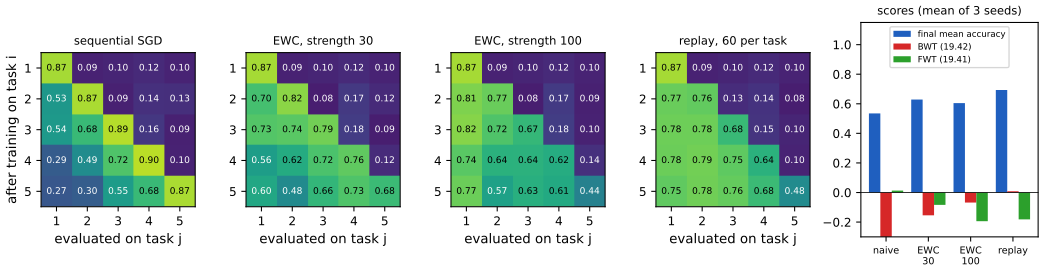
19.7.5 Online learning
pp. 763–765 Online learning differs from continual learning in the metric: learning and evaluation alternate at every step. The data-generating distribution \(p^\ast_t(x,y)=p(x\given\phi_t)p(y\given x,w_t)\) evolves (Figure 19.22, an influence diagram). At step \(t\) nature draws \((x_t,y_t)\sim p^\ast_t\); the agent sees \(x_t\) and predicts \(y_t\) with the posterior predictive \[ \hat p_{t\mid t-1}=p(y\given x_t,\D_{1:t-1}),\qquad\D_{1:t-1}=\{(x_s,y_s):s<t\},\tag{19.43} \] then pays a loss \[ L_t=\ell\big(\hat p_{t\mid t-1},y_t\big).\tag{19.44} \] This is prequential prediction (Dawid and Vovk, 1999) and underlies online conformal prediction (Vovk, Gammerman and Shafer, 2022). What matters is the cumulative loss \(L=\sum_{t\le T}L_t\), not the loss on a fixed test set. Two uses: for the log loss \(L\) is the negative log marginal likelihood (gap 19.16), giving a prequential minimum-description-length score for model selection (Dawid, 1984; Rissanen, 1984); and, especially when an adversary may generate the data, the cumulative loss is compared with the best one could have done in hindsight, the regret \[ \mathrm{regret}=\sum_{t=1}^T\Big[\ell\big(\hat p_{t\mid t-1},y_t\big)-\ell\big(\hat p_{t\mid T},y_t\big)\Big],\tag{19.45} \] where \(\hat p_{t\mid T}=p(y\given x_t,\D_{1:T})\) is the estimate fitted at the end. For convex losses regret bounds exist (gap 19.17; Orabona, 2019; Hazan, 2022), and they convert into bounds on the risk, the expected future loss (the argument is in the gap box below). Online learning is essential for decision and control, bandits (34.4) and reinforcement learning (Chapter 35), where there is no train-then-test split. The continual-learning scenarios are special cases of online learning: one distribution (task) per step, a batch of examples per step as input; on odd steps train and incur loss 0, on even steps evaluate on the union of the tasks seen (which recur) and return the empirical loss. In continual learning the data per task are large; online learning is more concerned with fast adaptation from small amounts of data per step to slowly or piecewise changing distributions.
Filling the gap 19.16: the cumulative log loss of the Bayesian predictor is the negative log marginal likelihood p. 763
Derivation
Take a model \(p(y_{1:T}\given x_{1:T})=\int\prod_tp(y_t\given x_t,\theta)\,p(\theta)\,\d\theta\) and the Bayesian predictive \(\hat p_{t\mid t-1}(y)=p(y\given x_t,\D_{1:t-1})\). By the chain rule of probability, \(p(y_{1:T}\given x_{1:T})=\prod_{t=1}^Tp(y_t\given x_{1:t},y_{1:t-1})\), and the conditional on the right is the posterior predictive \(\int p(y_t\given x_t,\theta)p(\theta\given\D_{1:t-1})\,\d\theta\) (given the past data \(\theta\) is independent of \(x_t\)). Taking the negative logarithm, \[ \sum_{t=1}^T-\log\hat p_{t\mid t-1}(y_t)=-\log p(y_{1:T}\given x_{1:T}), \] an exact identity: the log-loss paid online by the Bayesian is the negative log marginal likelihood, independently of the order of the data. Examples I confirm numerically. Bernoulli with a \(\mathrm{Beta}(a,b)\) prior: the predictive after \(k\) ones in \(t\) trials is \((k+a)/(t+a+b)\), and the product equals \(B(a+k_T,\,b+T-k_T)/B(a,b)\), the Beta-Bernoulli marginal likelihood. Bayesian linear regression with prior \(\N(0,\tau^2I)\) and noise variance \(\sigma^2\): the product of Gaussian predictives with variance \(\sigma^2+x_t^\T\Sigma_{t-1}x_t\) equals the Gaussian density \(\N(y;0,\sigma^2I+\tau^2XX^\T)\) of the whole response vector. Consequences. Comparing models by cumulative online log loss is comparing their marginal likelihoods (Bayes factors) and measures their combined fit and complexity (the prequential code length); it needs no held-out set. Where it fails. If the world drifts, a model that assumes an exchangeable sequence is mis-specified and the identity is then a statement about that model only: the cumulative loss can be dominated by the steps after a change, and a predictor that discounts the past (Figure 19.31c) is better even though it is not the Bayesian predictive of the stationary model.
Filling the gap 19.17: the regret of online gradient descent, and from regret to risk pp. 763–764
Derivation
Let \(\ell_t\) be convex with subgradients bounded by \(G\) (\(\|g_t\|\le G\), \(g_t\in\partial\ell_t(w_t)\)) on the ball \(K=\{w:\|w\|\le D\}\). Online gradient descent: \(w_1=0\), \(w_{t+1}=\Pi_K(w_t-\eta g_t)\) with \(\Pi_K\) the Euclidean projection. For any comparator \(u\in K\) (in particular the best fixed parameter in hindsight, \(u=\argmin_{K}\sum_t\ell_t\)), projection onto a convex set containing \(u\) does not increase the distance to \(u\), so \[ \|w_{t+1}-u\|^2\le\|w_t-\eta g_t-u\|^2=\|w_t-u\|^2-2\eta\,g_t^\T(w_t-u)+\eta^2\|g_t\|^2. \] Rearranging and using convexity, \(\ell_t(w_t)-\ell_t(u)\le g_t^\T(w_t-u)\le\dfrac{\|w_t-u\|^2-\|w_{t+1}-u\|^2}{2\eta}+\dfrac\eta2\|g_t\|^2\). Summing over \(t\) telescopes the first term: \[ \mathrm{Regret}_T=\sum_{t=1}^T\big[\ell_t(w_t)-\ell_t(u)\big]\le\frac{\|u\|^2}{2\eta}+\frac\eta2\sum_{t=1}^T\|g_t\|^2\le\frac{D^2}{2\eta}+\frac{\eta G^2T}2, \] and the choice \(\eta=D/(G\sqrt T)\) gives \(\mathrm{Regret}_T\le DG\sqrt T\): the average regret \(\mathrm{Regret}_T/T\) vanishes like \(1/\sqrt T\) for any sequence, even an adversarial one. For the logistic loss with \(\|x_t\|\le1\), \(G=1\). My implementation satisfies the first (sharper) inequality exactly on six random streams and the second with room to spare: Figure 19.31b shows regret about 36 at \(T=2000\) against the bound \(DG\sqrt T=89\). Strongly convex or exp-concave losses allow \(O(\log T)\) regret (Hazan, 2022); the Bayesian log loss of a Bernoulli stream has regret \(\tfrac12\log T+O(1)\) against the best fixed parameter (Krichevsky and Trofimov, 1981; Figure 19.31a), and the \(\mathrm{Beta}(\frac12,\frac12)\) prior satisfies \(\mathrm{regret}\le\frac12\ln T+\ln2\) for every sequence (I confirm exhaustively over all counts up to \(T=3000\)); the mean regret on a \(\theta=0.3\) stream tracks \(\frac12\ln T+\frac12\ln(\pi/2)\) (4.229 against 4.229 at \(T=3000\)).
From regret to risk. If the pairs are iid with risk \(R(w)=\E\,\ell(w;x,y)\), \(w_t\) is independent of the fresh pair at step \(t\), so \(\E[\ell_t(w_t)]=\E[R(w_t)]\). With the averaged iterate \(\bar w=\frac1T\sum_tw_t\), Jensen's inequality gives \(\E R(\bar w)\le\frac1T\sum_t\E R(w_t)=\frac1T\E\sum_t\ell_t(w_t)\le\frac1T\big(\E\sum_t\ell_t(u)+\mathrm{Regret}_T\big)=R(u)+\mathrm{Regret}_T/T\) for any fixed \(u\): a regret bound is a bound on the excess risk of the averaged iterate. (The book's (19.45) compares with the final-fit predictive rather than with the best fixed parameter; for the bounds above the comparator is the best fixed parameter in hindsight, the usual definition.)
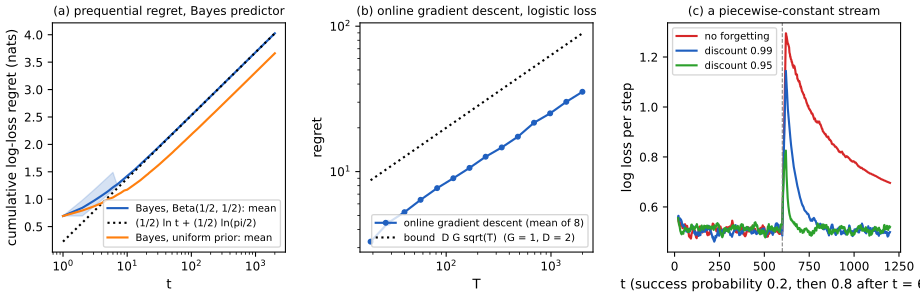
19.8 Adversarial examples
pp. 765–766 (The section is coauthored with Justin Gilmer.) Section 19.2 asked what happens when the input distribution moves for some reason. Here an adversary moves it deliberately. Given an input \(x\) classified as class \(c\), find a new input \(x^{\mathrm{adv}}\) that minimises the probability of that label, subject to being "perceptually similar" to \(x\): \[ x^{\mathrm{adv}}=\argmin_{x'\in\Delta(x)}\log p(y=c\given x'),\tag{19.46} \] where \(\Delta(x)\) is the set of inputs regarded as similar to \(x\). This is an adversarial attack (Figure 19.23, the panda classified as a gibbon after structured noise of size 0.007, is a photograph and is not reproduced). Szegedy et al. (2014) first noted how easily such inputs are found, which looks paradoxical given how well the same classifiers do on ordinary inputs; 19.8.5 resolves it. The security implications are real: Sharif et al. (2016) made a face recogniser mistake one person for another by means of patterned sunglasses, and Eykholt et al. (2018) made classifiers read stop signs as speed limits with small stickers. The book concentrates on deep networks for images, but logistic regression and generative models are also vulnerable, and so are audio and text.
19.8.1 Whitebox (gradient-based) attacks
p. 766 The attacker wants a small \(\delta\) such that \(x^{\mathrm{adv}}=x+\delta\) is classified as a chosen label \(y'\) (targeted) or as anything different from the current label (untargeted). In general the adversary maximises a loss, \[ x^{\mathrm{adv}}=\argmax_{x'\in\Delta(x)}L(x',y;\theta),\tag{19.47} \] with \(L=-\log p(y\given x')\) (untargeted) or \(L=\log p(y'\given x')\) (targeted), and "similar" usually means a bounded \(\ell_p\) ball, \[ \Delta(x)=\{x':\|x'-x\|_p<\epsilon\}.\tag{19.48} \] (The usual choices are \(p=2\) and \(p=\infty\); the book writes "\(p=1\) or \(p=0\)", see Notes on the book, item 6; the more realistic threat models of 19.8.3 do not fit this form.) In a whitebox attack the parameters \(\theta\) are known and any constrained optimiser can be used: bound-constrained BFGS (Szegedy et al., 2014), or the more efficient fast gradient sign method (FGS; Goodfellow, Shlens and Szegedy, 2015), \[ x_{t+1}=x_t+\delta_t,\qquad\delta_t=\epsilon\,\sign\big(\nabla_x\log p(y'\given x,\theta)\big|_{x_t}\big),\tag{19.49, 19.50} \] where the gradient is with respect to the pixels, not the weights, and \(\epsilon>0\) is a small step. Projected gradient descent (PGD; Madry et al., 2018) is the iterated version, projected back onto \(\Delta(x)\) after each step. No variant of PGD is best: the number of steps, the step size and the form of the loss matter, random restarts help to avoid local optima, and the loss should be monitored (Carlini et al., 2019).
Filling the gap 19.18: the fast gradient sign step is the exact solution of the linearised problem p. 766
Derivation
Linearise the loss around \(x\): \(L(x+\delta)\approx L(x)+g^\T\delta\) with \(g=\nabla_xL(x)\). The linearised attack is \(\max_{\|\delta\|_p\le\epsilon}g^\T\delta\). By Hölder's inequality \(g^\T\delta\le\|g\|_{p'}\|\delta\|_p\le\epsilon\|g\|_{p'}\) with \(\frac1p+\frac1{p'}=1\), and the bound is attained: for \(p=\infty\) (\(p'=1\)) at \(\delta=\epsilon\,\sign(g)\), since then \(g^\T\delta=\epsilon\sum_i|g_i|\); for \(p=2\) at \(\delta=\epsilon g/\|g\|_2\), giving \(\epsilon\|g\|_2\); for \(p=1\) (\(p'=\infty\)) at \(\delta=\epsilon\,\sign(g_k)e_k\) with \(k=\argmax_i|g_i|\), giving \(\epsilon\|g\|_\infty\). So (19.50) is the one-step maximiser of the first-order loss increase over an \(\ell_\infty\) ball (with the sign of the gradient of the log probability of the target label, or minus the sign of the gradient of the log probability of the true label, depending on whether the attack is targeted). Two remarks on (19.49): iterating it without projection can leave the \(\epsilon\)-ball after more than one step, which is why PGD projects; and the linearisation is a good approximation only if the loss is nearly linear over the ball.
A linear classifier: no approximation at all. For \(f(x)=w^\T x+b\) with label \(y\in\{-1,+1\}\) the margin \(m(x)=y\,f(x)\) is exactly linear in \(x\), so the worst case over \(\|\delta\|_p\le\epsilon\) is exact: \[ \min_{\|\delta\|_p\le\epsilon}y\,f(x+\delta)=y\,f(x)-\epsilon\|w\|_{p'}, \] attained at \(\delta=-\epsilon y\,\sign(w)\) for \(p=\infty\) (this is FGS) and at \(\delta=-\epsilon y\,w/\|w\|_2\) for \(p=2\). The prediction survives every perturbation in the ball iff \(y f(x)>\epsilon\|w\|_{p'}\), and the smallest perturbation that changes the label has \(\ell_p\) size \(|f(x)|/\|w\|_{p'}\), the distance to the hyperplane. I confirm both formulas by brute force over the \(2^8\) vertices of an \(\ell_\infty\) ball and by random search over an \(\ell_2\) ball.
Random against adversarial. A random perturbation \(\delta\) with independent signs \(\pm\epsilon\) changes the score by \(\epsilon\sum_iw_i\xi_i\), of standard deviation \(\epsilon\|w\|_2\), while the adversarial perturbation changes it by \(\epsilon\|w\|_1\); the ratio \(\|w\|_1/\|w\|_2\le\sqrt n\) can be large. For the logistic regression on 784 MNIST pixels fitted here (3 versus 8), \(\|w\|_1=103.7\) and \(\|w\|_2=5.92\), a factor 17.5, so a perturbation of size \(\epsilon=0.1\) per pixel moves the score by about \(0.1\times103.7=10.4\) in the worst case but only \(0.6\) typically. Figure 19.32a shows the consequence: the test accuracy falls from 96.7% to 7.6% at \(\epsilon=0.1\) under the exact attack (the same number as the FGS attack, since it is exact here), while random sign noise of the same size leaves it at about 95%.
19.8.2 Blackbox (gradient-free) attacks
p. 767 If the parameters are unknown (a blackbox attack) derivative-free optimisation (6.7) is used. Evolutionary algorithms produce fooling images (Nguyen, Yosinski and Clune, 2015): noise-like or patterned images (Figures 19.24 and 19.25) that a CNN classifies confidently; they are not realistic images, which distinguishes them from adversarial images. Su, Vargas and Sakurai (2019) attack by differential evolution on a single pixel, a perturbation with \(\|x^{\mathrm{adv}}-x\|_0=1\) (an \(\ell_0\) ball: a count of changed coordinates, not a norm). Papernot et al. (2017) fit a differentiable surrogate to the answers of the blackbox, attack the surrogate by gradients, and show that the attacks transfer to the real model, which compromised commercial image-classification services. None of this is computed here (the figures are photographs and images from large networks).
19.8.3 Real world adversarial attacks
p. 768 The set \(\Delta\) of admissible adversarial inputs is usually huge and cannot be described by a norm, because it depends on the attacker's goal. In the content-constrained threat model of Gilmer et al. (2018a) an attacker wants an image attachment that carries an advertisement but is not classified as spam: \(\Delta\) is all images containing that content, which spammers explore by changing fonts, orientations and background objects (Figure 19.26; Biggio et al., 2011), usually by hand with only limited-query access to the classifier. Optimisation can still explore parts of \(\Delta\).
19.8.4 Defenses based on robust optimization
p. 769 Because \(\Delta\) is so large, general security seems out of reach, but one can aim at models invariant to perturbations in a small constraint set \(\Delta(x)=\{x':\|x-x'\|_p<\epsilon\}\): a toy threat model with little security value but with benefits, as smoothness priors have improved robustness to random corruptions, transfer, and the features learned. The most direct approach is robust optimisation or adversarial training (Goodfellow, Shlens and Szegedy, 2015), which minimises the adversarial risk \[ \min_\theta\ \E_{(x,y)\sim p}\Big[\max_{x'\in\Delta(x)}L(x',y;\theta)\Big].\tag{19.51} \] It has a non-concave inner maximisation and a non-convex outer minimisation, and the inner problem is NP-hard in general (Katz et al., 2017), but in practice it suffices to take the gradient of the outer objective at an approximately maximal point \(x^{\mathrm{adv}}\approx\argmax_{x'}L(x',y;\theta)\) (Madry et al., 2018), found with a few PGD steps. Certified defenses prove that a model is robust in a region \(\Delta(x)\): randomised smoothing (Cohen, Rosenfeld and Kolter, 2019) turns a model that is robust to random Gaussian noise into one that is provably robust to bounded worst-case \(\ell_2\) perturbations; for ReLU networks the model is locally linear and certification in a region defined by linear constraints reduces to a series of linear programmes.
Filling the gap 19.19: adversarial training of a linear model in closed form, and why gradients at the maximiser are right (Danskin) p. 769
Derivation
(a) Linear models. Let \(\varphi\) be any non-increasing loss of the margin (logistic \(\varphi(m)=\log(1+e^{-m})\), hinge, exponential). Because the margin of \(x'=x+\delta\) is \(y f(x)+y w^\T\delta\) and its minimum over \(\|\delta\|_p\le\epsilon\) is \(y f(x)-\epsilon\|w\|_{p'}\) (gap 19.18), \[ \max_{\|\delta\|_p\le\epsilon}\varphi\big(y f(x+\delta)\big)=\varphi\big(y f(x)-\epsilon\|w\|_{p'}\big). \] So adversarial training (19.51) of a linear classifier is ordinary training with the margin reduced by \(\epsilon\|w\|_{p'}\): for \(\ell_\infty\) attacks the objective is \(\frac1N\sum_n\log\big(1+\exp(-y_nf(x_n)+\epsilon\|w\|_1)\big)\), and the inner maximum costs nothing. The term \(\epsilon\|w\|_1\) acts like an \(\ell_1\) penalty and produces sparse weights; for \(\ell_2\) attacks it is \(\epsilon\|w\|_2\), a norm penalty. This is what Figure 19.32 shows: the adversarially trained classifier (\(\epsilon=0.1\)) has \(\|w\|_1=10.0\) against 103.7 for the standard one and most weights are close to zero. (I confirm the closed form against a maximum over all vertices of the \(\ell_\infty\) ball for small dimension, and that my fitted solution is a local minimum of the penalised objective.) Cost: clean accuracy drops, 96.7% for the standard classifier, 95.3%, 92.7% and 84.8% for \(\epsilon_{\mathrm{train}}=0.05,0.1,0.2\), against robust accuracies at \(\epsilon=0.1\) of 79.7%, 83.5% and 79.5% (and 7.6% for the standard model): robustness is bought with accuracy.
(b) Danskin's theorem. Why is the gradient of \(\phi(\theta)=\max_{x\in K}L(x,\theta)\) equal to the gradient of \(L\) at the maximiser? Let \(K\) be compact, \(L\) and \(\nabla_\theta L\) jointly continuous, and suppose that for a given \(\theta\) the maximiser \(x^\ast\) is unique. Claim: \(\phi\) is differentiable at \(\theta\) and \(\nabla\phi(\theta)=\nabla_\theta L(x^\ast,\theta)\). Proof. Fix a direction \(v\). Lower bound: \(\phi(\theta+tv)\ge L(x^\ast,\theta+tv)\), so \(\frac{\phi(\theta+tv)-\phi(\theta)}t\ge\frac{L(x^\ast,\theta+tv)-L(x^\ast,\theta)}t\to\nabla_\theta L(x^\ast,\theta)^\T v\) as \(t\downarrow0\). Upper bound: let \(x_t\) maximise \(L(\cdot,\theta+tv)\). Then \(\phi(\theta+tv)-\phi(\theta)\le L(x_t,\theta+tv)-L(x_t,\theta)=t\,\nabla_\theta L(x_t,\theta+s_tv)^\T v\) for some \(s_t\in(0,t)\) (mean value theorem). Any limit point of \(x_t\) as \(t\to0\) maximises \(L(\cdot,\theta)\) by continuity, so by uniqueness \(x_t\to x^\ast\), and the right-hand side divided by \(t\) tends to \(\nabla_\theta L(x^\ast,\theta)^\T v\). The two bounds agree, so the one-sided directional derivative equals \(\nabla_\theta L(x^\ast,\theta)^\T v\); the argument for \(t\uparrow0\) is the same with the inequalities reversed, so the derivative is linear in \(v\) and \(\phi\) is differentiable. \(\square\) If the maximiser is not unique and \(L\) is convex in \(\theta\), \(\phi\) is convex and \(\nabla_\theta L(x^\ast,\theta)\) at any maximiser is a subgradient. This is why "PGD, then take the gradient at the point found" is a principled descent direction when the inner problem is solved well (and a heuristic when it is only approximately solved). I check numerically that the derivative of a maximum over a fine grid equals the partial derivative at the maximiser.
Filling the gap 19.20: randomised smoothing certifies an \(\ell_2\) radius (Neyman-Pearson) p. 769
Derivation
The book only names the method. Let \(f:\R^n\to\{1,\dots,K\}\) be any classifier (a network) and define the smoothed classifier \(g(x)=\argmax_cP_{\delta\sim\N(0,\sigma^2I)}[f(x+\delta)=c]\). Suppose at \(x\) the top class \(c_A\) has probability \(p_A=P[f(x+\delta)=c_A]>\frac12\) (so \(p_B\le1-p_A<\frac12\) for any other class).
Lemma (Gaussian shift). For any measurable \(A\subset\R^n\) with \(P[x+\delta\in A]=p\) and any shift \(v\), \(P[x+v+\delta\in A]\ge\Phi\big(\Phi^{-1}(p)-\|v\|/\sigma\big)\). Proof. Let \(P=\N(x,\sigma^2I)\) and \(Q=\N(x+v,\sigma^2I)\). The likelihood ratio is \(\frac{\d Q}{\d P}(z)=\exp\!\big(\frac{v^\T(z-x)}{\sigma^2}-\frac{\|v\|^2}{2\sigma^2}\big)\), an increasing function of the scalar \(t(z)=v^\T(z-x)/\|v\|\), and under \(P\), \(t\sim\N(0,\sigma^2)\). By the Neyman-Pearson lemma, among all sets with \(P(A)=p\) the set that minimises \(Q(A)\) is the one with the smallest likelihood ratios, \(A^\ast=\{z:t(z)\le\sigma\Phi^{-1}(p)\}\) (it has \(P(A^\ast)=p\)). Under \(Q\), \(t\sim\N(\|v\|,\sigma^2)\), so \(Q(A^\ast)=\Phi\big((\sigma\Phi^{-1}(p)-\|v\|)/\sigma\big)=\Phi(\Phi^{-1}(p)-\|v\|/\sigma)\). \(\square\)
Certificate. Apply the lemma to \(A=\{z:f(z)=c_A\}\): for every \(v\), \(P[f(x+v+\delta)=c_A]\ge\Phi(\Phi^{-1}(p_A)-\|v\|/\sigma)\), which is larger than \(\frac12=\Phi(0)\) as long as \(\|v\|<R=\sigma\Phi^{-1}(p_A)\). A class with probability above one half is the argmax, so \(g(x+v)=c_A\) for all \(\|v\|_2<\sigma\Phi^{-1}(p_A)\). (Cohen et al. refine this with both \(p_A\) and a bound \(p_B\) on the runner-up, \(R=\frac\sigma2\big(\Phi^{-1}(p_A)-\Phi^{-1}(p_B)\big)\ge\sigma\Phi^{-1}(p_A)\).) The radius is tight: for the halfspace classifier \(f(z)=\ind(a^\T z>b)\) with \(\|a\|=1\) and signed distance \(m=a^\T x-b>0\), \(p_A=\Phi(m/\sigma)\) and \(\sigma\Phi^{-1}(p_A)=m\) is exactly the distance to the decision boundary. I confirm the lemma on 30 random balls in \(\R^3\) (simulation within 0.004). In practice \(p_A\) is not known: it is replaced by a one-sided confidence lower bound from Monte Carlo samples of \(f(x+\delta)\) (Clopper-Pearson), and the method abstains if the bound does not exceed one half. The trade-off is in \(\sigma\): a larger \(\sigma\) gives a larger radius for the same \(p_A\), but the base classifier must then be accurate under heavier noise, which Figure 19.1 shows to be costly unless it is trained with noise (19.4.1).
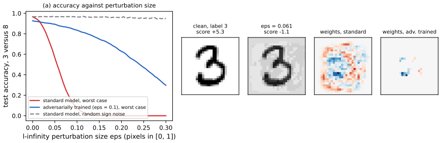
19.8.5 Why models have adversarial examples
pp. 769–770 The existence of adversarial inputs is paradoxical only if one forgets 19.2: it is a consequence of the lack of robustness to distribution shift. If a model's accuracy drops on some shifted input distribution \(p_{\mathrm{te}}(x)\) different from \(p_{\mathrm{tr}}(x)\), then errors exist, and if errors exist there is a nearest one, so the model is necessarily vulnerable to an adversary. In high dimension the nearest error is much closer than a randomly sampled error from \(p_{\mathrm{te}}\). Figure 19.27a is a cartoon: \(x_0\) is a clean image, \(B\) an image corrupted by Gaussian noise and \(A\) an adversarial image, with the set of errors \(E\) assumed (locally) a half-space. Let \(\mu=P_{\delta\sim\N(0,\sigma^2I)}[x_0+\delta\in E]\) be the error rate under noise at \(x_0\). For a half-space, \[ d(x_0,E)=-\sigma\,\Phi^{-1}(\mu),\tag{19.52} \] which in high dimension is far smaller than the typical distance to a noisy image, \(\|\delta\|_2\approx\sigma\sqrt n\). For ImageNet, \(n=224\times224\times3\) and \(\sigma=0.2\): with \(\mu=0.01\) the book computes \(d(x_0,E)\approx0.5\), more than 100 times closer than the noisy images at \(\sigma\sqrt n\approx77.6\). This small-volume error set near most points of a high-dimensional distribution is concentration of measure (Mahloujifar, Diochnos and Mahmoody, 2019; Gilmer et al., 2018b, "adversarial spheres"). The book's conclusion: there is nothing special about worst-case errors; they exist whenever errors exist.
Filling the gap 19.21: the derivation of (19.52) and what it implies pp. 769–770
Derivation
(19.52). Take the error set to be the half-space \(E=\{x:a^\T(x-x_0)\ge d\}\) with \(\|a\|_2=1\) and \(d=d(x_0,E)>0\) (the distance from \(x_0\) to \(E\) is the distance to the bounding hyperplane). For \(\delta\sim\N(0,\sigma^2I_n)\) the projection \(a^\T\delta\) is \(\N(0,\sigma^2)\) whatever \(n\) is (a unit linear functional of a spherical Gaussian), so \(\mu=P[a^\T\delta\ge d]=1-\Phi(d/\sigma)=\Phi(-d/\sigma)\), and solving, \(d=-\sigma\Phi^{-1}(\mu)\). I check by simulation that a half-space at \(d=-0.2\,\Phi^{-1}(0.01)=0.4653\) has error rate \(0.0100\) in noise for every dimension tried (Figure 19.33b).
The size of the noise. \(\|\delta\|^2/\sigma^2\sim\chi^2_n\), so \(\|\delta\|\) concentrates: its mean is \(\sigma\sqrt{n-\frac12}\,(1+o(1))\) and its standard deviation tends to \(\sigma/\sqrt2\), a constant that does not grow with \(n\) (3000 draws in \(n=1000\) give mean 6.318 and standard deviation 0.141 for \(\sigma=0.2\), against \(\sigma\sqrt{999.5}=6.323\) and \(\sigma/\sqrt2=0.141\)). The noise vector therefore lives on a thin shell at radius \(\approx\sigma\sqrt n\), while the half-space is at the fixed distance \(d\). The ratio \(\sigma\sqrt n/d\) grows like \(\sqrt n\): at \(n=150528\), \(\sigma=0.2\), \(\mu=0.01\), \(d=0.4653\) (the book rounds to 0.5), \(\sigma\sqrt n=77.60\) and the ratio is 167 (155 with the rounded 0.5), consistent with "more than 100 times". The two distances become equal only at \(n=(d/\sigma)^2\approx5.4\): in a handful of dimensions noise and adversary are comparable, which is the intuition behind the low-dimensional pictures that mislead.
What the formula implies for defence. Robustness at \(\ell_2\) radius \(r\) requires the error rate in noise to be at most \(\mu=\Phi(-r/\sigma)\) (from (19.52) with \(d=r\)): for \(r=0.5\) and \(\sigma=0.2\) that is \(\Phi(-2.5)=0.6\%\), and for \(r=2\) it is \(\Phi(-10)=7.6\times10^{-24}\). Making a classifier robust to a perturbation of norm \(r\) is therefore equivalent (under the half-space picture) to making errors in Gaussian noise of scale \(\sigma\) astronomically rare, which explains why adversarial robustness is hard even when ordinary accuracy and robustness to moderate random noise are high. Limits of the argument. The half-space is a local assumption (Figure 19.27b in the book shows a two-dimensional slice of an InceptionV3 decision boundary that looks like one); a curved error set changes constants but not the direction of the effect; and the argument is about \(\ell_2\) distances. The book's statement that "errors exist ⇒ nearest error exists" is trivially true; what (19.52) adds is a quantitative link between the error rate under noise and that nearest distance.
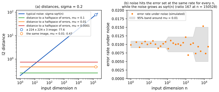
Try it: adversarial distance in high dimension, preset 1 is the ImageNet example; the second plot of that page uses the curves of Figure 19.32 for several adversarial-training strengths.
Supplement S19 (Beyond the iid assumption)
The supplement's Chapter 19 consists of the chapter title page only (its four pages are the title page, a blank page, the Part IV divider and a blank page); there is no additional material for this chapter in the draft.
Demonstrations
Practice problems
The book has no exercises for this chapter. These three short problems are my own.
Practice problem 19.1 (blackbox shift estimation by hand). A binary classifier has confusion matrix \(C=\begin{pmatrix}0.9&0.2\\0.1&0.8\end{pmatrix}\) on source data, whose prior is \((0.5,0.5)\). On \(n=1000\) unlabelled target points it predicts class 1 for 62% of them. (a) Estimate the target prior. (b) A target input has source posterior \(p(y=1\given x)=0.5\); what is \(q(y=1\given x)\)? (c) What is the standard deviation of \(\hat q_1\) if \(C\) is known?
Solution
(a) \(\mu=(0.62,0.38)\), \(\det C=0.72-0.02=0.70\), \(C^{-1}=\frac1{0.7}\begin{pmatrix}0.8&-0.2\\-0.1&0.9\end{pmatrix}\), so \(\hat q_1=(0.8\cdot0.62-0.2\cdot0.38)/0.7=0.42/0.7=0.6\) and \(\hat q_2=0.4\) (gap 19.10). (b) By (19.23) the posterior odds are multiplied by \(\frac{q_1/p_1}{q_2/p_2}=\frac{0.6/0.5}{0.4/0.5}=1.5\), so the odds go from 1 to 1.5 and \(q(y=1\given x)=0.6\). (c) With two classes \(\hat q_1=(\hat\mu_1-0.2)/0.7\), so \(\mathrm{sd}(\hat q_1)=\sqrt{\mu_1(1-\mu_1)/n}/0.7=\sqrt{0.62\cdot0.38/1000}/0.7=0.0153/0.7=0.0219\). The estimate is 0.60 with a standard error of about 0.022, three times larger than that of the raw fraction (0.0153), the price of correcting for the classifier's errors.
Practice problem 19.2 (importance weights and the effective sample size). Source \(p=\N(0,1)\), target \(q=\N(m,1)\). (a) Show that a balanced logistic regression recovers \(h(x)=mx-m^2/2\) and that the weights are \(w=e^{mx-m^2/2}\). (b) Compute \(\E_p[w^2]\) and the effective sample size fraction. (c) For which \(m\) is it 10%?
Solution
(a) \(\log\frac{q(x)}{p(x)}=-\frac{(x-m)^2}2+\frac{x^2}2=mx-\frac{m^2}2\), linear in \(x\), so the classifier with features \((1,x)\) is well specified and (19.18) gives \(w=e^{h}\) (gap 19.8). (b) \(\E_p[w^2]=\int e^{2mx-m^2}\frac{e^{-x^2/2}}{\sqrt{2\pi}}\d x=e^{-m^2}e^{2m^2}=e^{m^2}\) (the moment generating function of a standard normal at \(2m\) is \(e^{2m^2}\)), so \(\mathrm{ESS}/N\approx1/\E_p[w^2]=e^{-m^2}\); for \(m=1\) it is 0.368. (c) \(e^{-m^2}=0.1\) gives \(m=\sqrt{\ln10}=1.517\): a shift of one and a half standard deviations already throws away 90% of the sample. My code gives \(e^{-m^2}\) from the general closed form of gap 19.7 with \(s_p=s_q=1\).
Practice problem 19.3 (the exact attack on a two-pixel classifier). The classifier \(f(x)=3x_1-4x_2\), label \(y=+1\), input \(x=(1,0.5)\). (a) How large must an \(\ell_2\) and an \(\ell_\infty\) perturbation be to flip the prediction? (b) Give the FGS point at the flipping \(\epsilon\). (c) If instead independent noise \(\N(0,0.1^2)\) is added to each coordinate, with what probability does the prediction flip?
Solution
(a) \(f(x)=3-2=1\), \(\|w\|_2=5\), \(\|w\|_1=7\). The distance to the hyperplane is \(f/\|w\|_{p'}\): \(1/5=0.2\) in \(\ell_2\) (\(p'=2\)) and \(1/7=0.143\) in \(\ell_\infty\) (\(p'=1\)) (gap 19.18). (b) \(\delta=-\epsilon y\sign(w)=-\epsilon(1,-1)\), so at \(\epsilon=1/7\), \(x^{\mathrm{adv}}=(1-\frac17,\,0.5+\frac17)=(0.857,0.643)\) with score \(3(0.857)-4(0.643)=0\). (c) The score changes by \(w^\T\delta\sim\N(0,0.1^2\cdot25)=\N(0,0.5^2)\), so the prediction flips when this is below \(-1\): probability \(\Phi(-1/0.5)=\Phi(-2)=0.0228\). Random noise of per-coordinate sd 0.1 (an \(\ell_2\) size about 0.14) flips the label in 2.3% of draws; the adversary flips it for sure with an \(\ell_\infty\) size of 0.143 and an \(\ell_2\) size of 0.2, a perturbation no larger than a typical noise draw.
Notes on the book
Slips and sharpenings found while proving and checking the claims
- Section 19.3.2.2, the energy score. The text defines the logits as \(\ell_c=\log p_c\) and gives the energy score as \(s=\sum_c\ell_c\). The energy score of Liu et al. (2020) is the negative log-sum-exp of the unnormalised logits \(z_c\), \(E(x)=-T\log\sum_ce^{z_c/T}\). With normalised log probabilities the log-sum-exp is identically \(\log1=0\), and a sum of log probabilities is not an energy at all; the score should be \(\lse(z_{1:C})\) of the logits \(z\) (up to sign).
- Equation (19.19), domain-adversarial learning. As printed, \(\min_\gamma\max_{\alpha,\beta}\) of (domain loss + label loss) has the domain classifier \(c_\beta\) maximising its own domain-classification loss, and the feature extractor \(\alpha\) only maximising, although the label loss also depends on \(\alpha\). The intended saddle point (Ganin et al., 2016) is: the domain classifier \(\beta\) minimises the domain loss, and the extractor and the label head \((\alpha,\gamma)\) minimise the label loss minus (a multiple of) the domain loss: \(\min_{\alpha,\gamma}\max_\beta[L_y-\lambda L_d]\), which is what the gradient-reversal layer implements (gap 19.9).
- Equation (19.22). The sum \(\mu_i=\sum_iC_{ij}q_j\) should be over \(j\). Also, the requirement for \(C\) to be invertible, "the model predicts class \(y_i\) correctly more often than any other class \(y_j\)", is not sufficient: a matrix whose diagonal entry is the largest in its column can be singular (the example of gap 19.10(b)); a sufficient condition is that every class is classified correctly more than half the time (\(C_{jj}>\frac12\), strict column diagonal dominance).
- Equations (19.30) and (19.31). They carry \(\argmin\) but are expectations of \(\log q_\phi\) with a positive sign: minimising the expected KL divergence (19.29) is maximising \(\E[\log q_\phi]\) (the KL is \(\E_p\log p-\E_p\log q_\phi\)), so \(\argmin\) should be \(\argmax\) (or the expressions need a minus sign). The Monte Carlo objective (19.32) is correctly a quantity to maximise (gap 19.13).
- Equations (19.41) and (19.42). The text describes forward transfer as the benefit of earlier tasks for later ones "beyond what would have been obtained from scratch", but (19.41) compares \(R_{j,j}\), performance just after training on task \(j\), with \(R^{\mathrm{ind}}_j\); in Lopez-Paz and Ranzato (2017) the forward transfer compares the performance on task \(j\) before training on it, \(R_{j-1,j}\), with a baseline of a randomly initialised model, and the sums run over \(T-1\) terms. The BWT average over \(T\) includes the term \(j=T\), which is zero, so (19.42) is \((T-1)/T\) times the Lopez-Paz and Ranzato value. I use the definitions as printed (Figure 19.30).
- Equation after (19.48). "Typically people assume \(p=1\) or \(p=0\)": the usual choices are \(p=2\) and \(p=\infty\) (the FGS step (19.50) is the \(\ell_\infty\) one); \(\ell_0\), the number of changed coordinates, is not a norm and is the threat model of the one-pixel attack of 19.8.2.
- Section 19.8.5. The noise is written \(\delta\sim\N(0,\sigma I)\); the covariance is \(\sigma^2I\) (the book's \(\|\delta\|_2\approx\sigma\sqrt d\) uses \(\sigma^2I\)). Also (19.52) with \(\sigma=0.2\), \(\mu=0.01\) gives \(d(x_0,E)=0.465\), which the text rounds to 0.5; the ratio to \(\sigma\sqrt n=77.6\) is then 167, not just "more than 100" (still correct).
- Section 19.8.1, equation (19.49). Iterating \(x_{t+1}=x_t+\delta_t\) with a fixed \(\epsilon\) does not keep the iterates in the \(\epsilon\)-ball: after \(k\) steps the \(\ell_\infty\) distance can be \(k\epsilon\). One step is the FGS attack; the multi-step version needs the projection of PGD. Also, in 19.3.2.3 the type-I risk \(R_1\) is controlled by a calibration quantile exactly (gap 19.2); the joint control of \(R_1\) and \(R_2\) needs the multiple-testing argument of the cited paper.
References
- Murphy, K. P. (2023). Probabilistic Machine Learning: Advanced Topics. MIT Press, Cambridge, MA. Chapter 19, pp. 735–770. probml.github.io/pml-book/book2.html.
- Ahuja, K., Caballero, E., Zhang, D., Gagnon-Audet, J.-C., Bengio, Y., Mitliagkas, I. and Rish, I. (2021). Invariance principle meets information bottleneck for out-of-distribution generalization. NeurIPS, 34.
- Angelopoulos, A. N., Bates, S., Candès, E. J., Jordan, M. I. and Lei, L. (2021). Learn then test: calibrating predictive algorithms to achieve risk control. arXiv:2110.01052.
- Arjovsky, M., Bottou, L., Gulrajani, I. and Lopez-Paz, D. (2019). Invariant risk minimization. arXiv:1907.02893.
- Baxter, J. (2000). A model of inductive bias learning. Journal of Artificial Intelligence Research, 12, 149–198.
- Ben-David, S., Blitzer, J., Crammer, K., Kulesza, A., Pereira, F. and Vaughan, J. W. (2010). A theory of learning from different domains. Machine Learning, 79, 151–175.
- Bendale, A. and Boult, T. (2015). Towards open world recognition. CVPR.
- Biggio, B., Fumera, G., Pillai, I. and Roli, F. (2011). A survey and experimental evaluation of image spam filtering techniques. Pattern Recognition Letters, 32(10), 1436–1446.
- Bishop, C. M. (1995). Training with noise is equivalent to Tikhonov regularization. Neural Computation, 7(1), 108–116.
- Carlini, N., Athalye, A., Papernot, N., Brendel, W., Rauber, J., Tsipras, D., Goodfellow, I., Madry, A. and Kurakin, A. (2019). On evaluating adversarial robustness. arXiv:1902.06705.
- Caruana, R. (1997). Multitask learning. Machine Learning, 28, 41–75.
- Cohen, J., Rosenfeld, E. and Kolter, J. Z. (2019). Certified adversarial robustness via randomized smoothing. ICML.
- Dawid, A. P. (1984). Present position and potential developments: some personal views, statistical theory, the prequential approach. Journal of the Royal Statistical Society A, 147(2), 278–292.
- Dawid, A. P. and Vovk, V. G. (1999). Prequential probability: principles and properties. Bernoulli, 5(1), 125–162.
- De Lange, M. and Tuytelaars, T. (2021). Continual prototype evolution: learning online from non-stationary data streams. ICCV.
- Domke, J. and Sheldon, D. (2018). Importance weighting and variational inference. NeurIPS, 31.
- Eykholt, K. et al. (2018). Robust physical-world attacks on deep learning visual classification. CVPR.
- Feng, S. Y. et al. (2021). A survey of data augmentation approaches for NLP. Findings of ACL.
- Finn, C., Abbeel, P. and Levine, S. (2017). Model-agnostic meta-learning for fast adaptation of deep networks. ICML.
- French, R. M. (1999). Catastrophic forgetting in connectionist networks. Trends in Cognitive Sciences, 3(4), 128–135.
- Ganin, Y. et al. (2016). Domain-adversarial training of neural networks. Journal of Machine Learning Research, 17(59), 1–35.
- Garg, S., Wu, Y., Balakrishnan, S. and Lipton, Z. (2020). A unified view of label shift estimation. NeurIPS, 33.
- Garnelo, M. et al. (2018). Neural processes. arXiv:1807.01622.
- Geng, C., Huang, S.-J. and Chen, S. (2020). Recent advances in open set recognition: a survey. IEEE TPAMI.
- Gilmer, J. et al. (2018a). Motivating the rules of the game for adversarial example research. arXiv:1807.06732.
- Gilmer, J., Metz, L., Faghri, F., Schoenholz, S. S., Raghu, M., Wattenberg, M. and Goodfellow, I. (2018b). Adversarial spheres. arXiv:1801.02774.
- Goodfellow, I. J., Shlens, J. and Szegedy, C. (2015). Explaining and harnessing adversarial examples. ICLR.
- Gordon, J., Bronskill, J., Bauer, M., Nowozin, S. and Turner, R. E. (2019). Meta-learning probabilistic inference for prediction. ICLR.
- Goyal, S., Sun, M., Raghunathan, A. and Kolter, J. Z. (2022). Test-time adaptation via conjugate pseudo-labels. NeurIPS, 35.
- Gulrajani, I. and Lopez-Paz, D. (2021). In search of lost domain generalization. ICLR.
- Hazan, E. (2022). Introduction to Online Convex Optimization, 2nd edition. MIT Press.
- Hospedales, T., Antoniou, A., Micaelli, P. and Storkey, A. (2022). Meta-learning in neural networks: a survey. IEEE TPAMI, 44(9), 5149–5169.
- Hu, X. and Lei, J. (2020). A distribution-free test of covariate shift using conformal prediction. arXiv:2010.07147.
- Katz, G., Barrett, C., Dill, D. L., Julian, K. and Kochenderfer, M. J. (2017). Reluplex: an efficient SMT solver for verifying deep neural networks. CAV.
- Kirkpatrick, J. et al. (2017). Overcoming catastrophic forgetting in neural networks. PNAS, 114(13), 3521–3526.
- Krichevsky, R. E. and Trofimov, V. K. (1981). The performance of universal encoding. IEEE Transactions on Information Theory, 27(2), 199–207.
- Lipton, Z., Wang, Y.-X. and Smola, A. (2018). Detecting and correcting for label shift with black box predictors. ICML.
- Liu, W., Wang, X., Owens, J. and Li, Y. (2020). Energy-based out-of-distribution detection. NeurIPS, 33.
- Lopez-Paz, D. and Ranzato, M. (2017). Gradient episodic memory for continual learning. NeurIPS, 30.
- Madry, A., Makelov, A., Schmidt, L., Tsipras, D. and Vladu, A. (2018). Towards deep learning models resistant to adversarial attacks. ICLR.
- Mahloujifar, S., Diochnos, D. I. and Mahmoody, M. (2019). The curse of concentration in robust learning: evasion and poisoning attacks from concentration of measure. AAAI.
- Misra, I., Shrivastava, A., Gupta, A. and Hebert, M. (2016). Cross-stitch networks for multi-task learning. CVPR.
- Morningstar, W. R., Alemi, A. A. and Dillon, J. V. (2020). PACm-Bayes: narrowing the empirical risk gap in the misspecified Bayesian regime. arXiv:2010.09629.
- Nguyen, A., Yosinski, J. and Clune, J. (2015). Deep neural networks are easily fooled: high confidence predictions for unrecognizable images. CVPR.
- Orabona, F. (2019). A modern introduction to online learning. arXiv:1912.13213.
- Papernot, N., McDaniel, P., Goodfellow, I., Jha, S., Celik, Z. B. and Swami, A. (2017). Practical black-box attacks against machine learning. ACM AsiaCCS.
- Peters, J., Bühlmann, P. and Meinshausen, N. (2016). Causal inference by using invariant prediction: identification and confidence intervals. Journal of the Royal Statistical Society B, 78(5), 947–1012.
- Rabanser, S., Günnemann, S. and Lipton, Z. (2019). Failing loudly: an empirical study of methods for detecting dataset shift. NeurIPS, 32.
- Ren, J. et al. (2019). Likelihood ratios for out-of-distribution detection. NeurIPS, 32.
- Rissanen, J. (1984). Universal coding, information, prediction, and estimation. IEEE Transactions on Information Theory, 30(4), 629–636.
- Robins, A. (1995). Catastrophic forgetting, rehearsal and pseudorehearsal. Connection Science, 7(2), 123–146.
- Rosenfeld, E., Ravikumar, P. and Risteski, A. (2021). The risks of invariant risk minimization. ICLR.
- Saerens, M., Latinne, P. and Decaestecker, C. (2002). Adjusting the outputs of a classifier to new a priori probabilities: a simple procedure. Neural Computation, 14(1), 21–41.
- Salehi, M., Mirzaei, H., Hendrycks, D., Li, Y., Rohban, M. H. and Sabokrou, M. (2022). A unified survey on anomaly, novelty, open-set, and out-of-distribution detection. Transactions on Machine Learning Research.
- Sharif, M., Bhagavatula, S., Bauer, L. and Reiter, M. K. (2016). Accessorize to a crime: real and stealthy attacks on state-of-the-art face recognition. ACM CCS.
- Shimodaira, H. (2000). Improving predictive inference under covariate shift by weighting the log-likelihood function. Journal of Statistical Planning and Inference, 90(2), 227–244.
- Shorten, C. and Khoshgoftaar, T. M. (2019). A survey on image data augmentation for deep learning. Journal of Big Data, 6, 60.
- Snell, J., Swersky, K. and Zemel, R. (2017). Prototypical networks for few-shot learning. NeurIPS, 30.
- Storkey, A. (2009). When training and test sets are different: characterizing learning transfer. In Dataset Shift in Machine Learning, MIT Press.
- Su, J., Vargas, D. V. and Sakurai, K. (2019). One pixel attack for fooling deep neural networks. IEEE Transactions on Evolutionary Computation, 23(5), 828–841.
- Sugiyama, M., Krauledat, M. and Müller, K.-R. (2007). Covariate shift adaptation by importance weighted cross validation. Journal of Machine Learning Research, 8, 985–1005.
- Sun, Y., Wang, X., Liu, Z., Miller, J., Efros, A. and Hardt, M. (2020). Test-time training with self-supervision for generalization under distribution shifts. ICML.
- Szegedy, C. et al. (2014). Intriguing properties of neural networks. ICLR.
- Thrun, S. and Pratt, L. (eds.) (1998). Learning to Learn. Springer.
- Vaze, S., Han, K., Vedaldi, A. and Zisserman, A. (2022). Open-set recognition: a good closed-set classifier is all you need? ICLR.
- Vovk, V., Gammerman, A. and Shafer, G. (2022). Algorithmic Learning in a Random World, 2nd edition. Springer.
- Wang, D., Shelhamer, E., Liu, S., Olshausen, B. and Darrell, T. (2021). Tent: fully test-time adaptation by entropy minimization. ICLR.
- Widmer, G. and Kubat, M. (1996). Learning in the presence of concept drift and hidden contexts. Machine Learning, 23, 69–101.
- Xie, S. M., Raghunathan, A., Liang, P. and Ma, T. (2022). An explanation of in-context learning as implicit Bayesian inference. ICLR.
- Zhang, M., Levine, S. and Finn, C. (2022). MEMO: test time robustness via adaptation and augmentation. NeurIPS, 35.
- Zhang, Y. and Yang, Q. (2021). A survey on multi-task learning. IEEE Transactions on Knowledge and Data Engineering.
- Zhou, A. and Levine, S. (2021). Bayesian adaptation for covariate shift. NeurIPS, 34.
- Zhuang, F. et al. (2021). A comprehensive survey on transfer learning. Proceedings of the IEEE, 109(1), 43–76.
The numerical statements in the text (the selection-bias effects, the noise-augmentation identity and the capped-weight DRO identity, the importance-weight identities, effective sample sizes and the Gaussian closed form, the logistic density-ratio recovery and its unequal-sample correction, the fine-tuning closed form and its risk, the domain-discrepancy bound and the Jensen-Shannon identity, the blackbox shift moment equation, its covariance, the singular-matrix example and the EM estimate, the marginal-entropy identity and the entropy gradient, the exact spurious-feature risks and the IRM solution, the prototypical-network equivalence, the prequential identities, the regret bounds, the continual-learning results, the OOD likelihood experiments, the conformal false-flag rate, the exact adversarial attacks and adversarial training, Danskin's derivative, the concentration numbers, the smoothing radius and the practice problems) were confirmed numerically.