Deep neural networks
A deep neural network is a differentiable function written as a graph of simple blocks. This short chapter lists the blocks (linear, convolutional, residual, normalising, dropout, attention, recurrent, multiplicative and implicit layers) and the architectures built from them (MLPs, CNNs, autoencoders, RNNs, transformers and graph networks). The notes keep the book's order, add the supplement's transformer and graph sections where they belong, and prove the facts the text only states: why a stack of linear layers collapses, why residual connections keep gradients alive, what layer normalisation and dropout really compute, why attention is kernel regression, and why a transformer is a graph network on a complete graph.
Ch. 1 Introduction Ch. 2 Probability Ch. 3 Statistics Ch. 4 Graphical models Ch. 5 Information theory Ch. 6 Optimisation Ch. 7 Inference algorithms Ch. 8 Gaussian filtering Ch. 9 Message passing Ch. 10 Variational inference Ch. 11 Monte Carlo Ch. 12 MCMC Ch. 13 Sequential Monte Carlo Ch. 14 Predictive models Ch. 15 GLMs Ch. 16 Deep networks Ch. 17 Bayesian neural networks Ch. 18 Gaussian processes Ch. 19 Beyond iid Ch. 20 Generative models Ch. 21 VAEs Ch. 22 Autoregressive models Ch. 23 Normalizing flows Ch. 24 Energy-based models Ch. 25 Diffusion models Ch. 26 GANs Ch. 27 Discovery methods Ch. 28 Latent factor models Ch. 29 State-space models Ch. 30 Graph learning Ch. 31 Nonparametric Bayes Ch. 32 Representation learning Ch. 33 Interpretability Ch. 34 Decision making Ch. 35 Reinforcement learning Ch. 36 Causality
How to read these notes
They follow the book. Sections carry the book's numbers and equations keep theirs (for example (16.12) and (16.22)). The supplement's Sections 16.1.1 (transformers) and 16.1.2 (graph neural networks) are placed under the main-text Sections 16.3.5 and 16.3.6 and marked (supplement); the supplement numbers its own equations from (16.1), so I quote them as "supplement (16.1)".
Filling the gaps. Wherever the book states a result without proof, an orange Filling the gap box gives the full argument. Proofs start hidden.
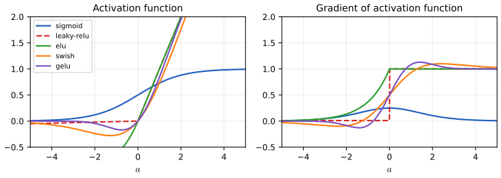
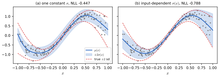
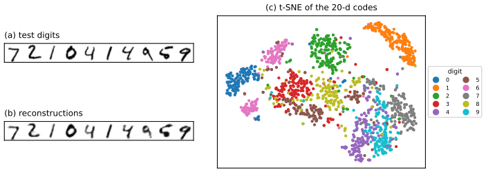
Figures. Figure 16.2 (activations and their gradients) is reproduced exactly. Figure 16.14 is reproduced with a smaller training set and fewer epochs than the book's notebook (the caption says so). All other figures of the chapter and the supplement are drawings with nothing computed (neurons, diagrams of layers and blocks, graph illustrations); the facts they illustrate are confirmed in code instead. One own figure shows the two-head regression of Section 16.3.1.
Demos. Three interactive pages: attention as a soft lookup, a mean head and a variance head, message passing on graphs.
Main reference
K. P. Murphy, Probabilistic Machine Learning: Advanced Topics, MIT Press (2023; December 2025 draft), Chapter 16, pages 631–646, and Supplement Chapter 16, pages 173–180 (book page: probml.github.io/pml-book/book2.html). The chapter has no exercises; three practice problems at the end are my own.
Companion courses
- Probabilistic Machine Learning: An Introduction: Chapter 13 neural networks for tabular data (MLPs, activations, backpropagation, residual connections, regularisation), Chapter 14 images (convolution, pooling, normalisation) and Chapter 15 sequences (RNNs, attention, transformers).
- Foundations of Deep Learning: Chapter 6 deep networks, Chapter 8 backpropagation, Chapter 9 regularisation (residuals, dropout), Chapter 10 convolutional networks, Chapter 12 transformers, Chapter 13 graph networks, Chapter 19 autoencoders.
- This course: Chapter 6, Section 6.2 automatic differentiation (the gradients of these graphs), Chapter 9 message passing (belief propagation, which a GNN generalises).
What this chapter adds: a catalogue of the blocks from which later chapters build models (Bayesian neural networks in Chapter 17, deep generative models in Chapters 20 to 26), and proofs of the properties that make the blocks work.
The chapter at a glance
- 16.2 Blocks: linear and nonlinear layers (gap 16.1, 16.2), convolution (16.3), residual connections (16.4), normalisation (16.5), dropout (16.6), attention (16.7), multiplicative layers (16.9), implicit layers (16.10).
- 16.3 Architectures: MLPs with two heads (gap 16.11), CNNs, autoencoders (16.12), RNNs (16.8), transformers (16.13) and graph networks (16.14, 16.15).
Notation. \(x\) is the input of a block and \(y\) its output; \(W,b\) weights and biases; \(\varphi\) an elementwise activation; \(\sigma(a)=1/(1+e^{-a})\); \(\Phi,\phi\) the standard normal cdf and density; \(Q,K,V\) queries, keys and values with \(d_k,d_v\) their widths; \(A\) an adjacency matrix and \(\nbr(i)\) the neighbours of node \(i\).
16.1 Introduction
p. 631 In its modern use, a deep neural network (DNN) is any differentiable function that can be written as a computation graph: nodes are primitive operations (a matrix product, an elementwise nonlinearity) and edges carry vectors, matrices or tensors. The simplest graph is a chain of layers, and "deep" means many of them. Fitting such a function to data by gradient-based minimisation of a loss is deep learning; the gradients come from reverse-mode differentiation (Chapter 6, Section 6.2; proofs in Foundations of Deep Learning, Chapter 8).
Networks combine with probabilistic models in two ways. First, as nonlinear functions inside conditional distributions, for example a classifier \(p(y\given x,\theta)=\operatorname{Cat}(y\given\softmax(f(x;\theta)))\) or a directed graphical model whose conditional distributions are networks. Second, as inference networks that output an approximate posterior \(q(z\given f(\mathcal D;\phi))\) (amortised inference; the Bayesian treatment of the weights is Chapter 17).
16.2 Building blocks of differentiable circuits
p. 632 This section lists the node types. The input to a block is \(x\) and its output \(y\).
16.2.1 Linear layers
p. 632 A single neuron computes the real number \(y=w^{\T}x+b\) (16.1), with parameters \(\theta=(w,b)\). A layer of units stacks several neurons into the linear (or fully connected) layer \[ y=f(x;\theta)=Wx+b,\qquad\theta=(W,b). \tag{16.2} \] The bias can be absorbed: with \(\tilde W=[W,b]\) and \(\tilde x=[x,1]\), \(y=\tilde W\tilde x\), so formulas may drop \(b\) without loss.
16.2.2 Nonlinearities
pp. 632–633 A stack of linear layers is still one linear layer (gap 16.1), so each layer is followed by an elementwise activation function \(\varphi\): \[ y=\varphi(x)=[\varphi(x_1),\dots,\varphi(x_D)]. \tag{16.3} \] Table 16.1 lists the common choices: sigmoid \(\sigma(a)\), \(\tanh a=2\sigma(2a)-1\), softplus \(\log(1+e^a)\), \(\relu(a)=\max(a,0)\), leaky ReLU \(\max(a,0)+\alpha\min(a,0)\), ELU \(\max(a,0)+\min(\alpha(e^a-1),0)\), swish \(a\sigma(a)\), GELU \(a\Phi(a)\) and the sine \(\sin a\). Their elementary properties are proved in gap 16.2.
Filling the gap 16.1: a stack of linear layers is one linear layer p. 632
Derivation
Take two affine layers \(y_1=W_1x+b_1\) and \(y_2=W_2y_1+b_2\) with compatible shapes. Substituting, \(y_2=W_2W_1x+(W_2b_1+b_2)\), which is again affine with weight \(W_2W_1\) and bias \(W_2b_1+b_2\). By induction on the number of layers, \(L\) affine layers compute \(x\mapsto(W_L\cdots W_1)x+b\) for some vector \(b\). Hence the set of functions represented by the stack is contained in the set represented by one layer, and extra depth adds no expressive power unless a nonlinearity sits between the layers. The product \(W_L\cdots W_1\) does have rank at most \(\min_l\operatorname{rank}W_l\), so a stack with a narrow layer is a low-rank linear map, which is the (only) effect depth has in the linear case.
With the activation \(\relu\) the picture changes: \(\relu\) is continuous and piecewise linear, and compositions, sums and maxima of continuous piecewise linear functions are again continuous piecewise linear, so a ReLU network is a continuous piecewise-linear function whose linear pieces are different affine maps on different regions of the input space; the universal approximation theorem and its proof are in Foundations of Deep Learning, Section 6.2.2.
See also: differentiable MLPs and activation functions in the Introduction volume.
Filling the gap 16.2: identities and derivatives of the activation functions Table 16.1, Figure 16.2
Derivation
tanh and the sigmoid. \(\tanh a=\frac{e^a-e^{-a}}{e^a+e^{-a}}=\frac{2}{1+e^{-2a}}-1=2\sigma(2a)-1\), multiplying numerator and denominator by \(e^{-a}\).
Derivatives. \(\sigma'(a)=\frac{e^{-a}}{(1+e^{-a})^2}=\sigma(a)(1-\sigma(a))\). By AM-GM, \(\sigma(1-\sigma)\le\big(\frac{\sigma+(1-\sigma)}{2}\big)^2=\frac14\), with equality iff \(\sigma=\tfrac12\), that is \(a=0\); so \(0<\sigma'\le\frac14\). From the chain rule and the identity above, \(\tanh'(a)=4\sigma'(2a)=4\sigma(2a)(1-\sigma(2a))=(1+t)(1-t)=1-t^2\) with \(t=\tanh a\), so \(0<\tanh'\le1\). Softplus: \(\frac{\d}{\d a}\log(1+e^a)=\frac{e^a}{1+e^a}=\sigma(a)\). Swish: \((a\sigma)'=\sigma+a\sigma(1-\sigma)\). GELU: \((a\Phi)'=\Phi(a)+a\phi(a)\). ELU: \(1\) for \(a>0\) and \(\alpha e^a\) for \(a<0\). ReLU and leaky ReLU have derivative \(1\) for \(a>0\) and \(0\) (respectively \(\alpha\)) for \(a<0\); at \(a=0\) any value in the subdifferential may be used.
Why saturating activations hurt depth. By the chain rule the gradient through \(L\) sigmoid layers contains the factor \(\prod_l\sigma'(a_l)\le4^{-L}\), which vanishes exponentially (this is the vanishing-gradient problem; ReLU has derivative \(1\) on its active side).
Softplus is a smooth ReLU. For \(a\ge0\), \(\log(1+e^a)-a=\log(1+e^{-a})\); for \(a<0\), \(\log(1+e^a)-0=\log(1+e^{-|a|})\) too. Hence \(0<\softplus(a)-\relu(a)=\log(1+e^{-|a|})\le\log2\), with the maximum at \(a=0\). Scaling, \(\frac1\beta\softplus(\beta a)\) differs from \(\relu(a)\) by at most \((\log 2)/\beta\) and converges uniformly to it as \(\beta\to\infty\).
Ranges. Table 16.1 lists the range of ELU, swish and GELU as \([-\infty,\infty]\), but they are bounded below: ELU by \(-\alpha\); swish by \(-0.2785\) (attained at \(a\approx-1.278\)) and GELU by \(-0.1700\) (at \(a\approx-0.752\)), found by solving \(\text{swish}'=0\) and \(\text{GELU}'=0\) numerically. Both are non-monotone, unlike the others.
16.2.3 Convolutional layers
pp. 633–634 For image data one applies the same small weight matrix (the kernel or filter) to every local patch. For an image \(X\in\R^{H\times W}\) and kernel \(w\in\R^{h\times w}\) the output \(Z=X\circledast w\) is \[ Z_{i,j}=\sum_{u=0}^{h-1}\sum_{v=0}^{w-1}x_{i+u,\,j+v}\,w_{u,v}. \tag{16.4} \] (Strictly this is cross-correlation, but deep learning calls it convolution.) With no padding the output has size \((H-h+1)\times(W-w+1)\). With \(C\) input channels and \(D\) output channels there are \(D\) kernels of size \(h\times w\times C\) and \[ z_{i,j,d}=\sum_{u=0}^{h-1}\sum_{v=0}^{w-1}\sum_{c=0}^{C-1}x_{i+u,\,j+v,\,c}\,w_{u,v,c,d}. \tag{16.5} \] Figure 16.3 shows a \(6\times6\times3\) input and two \(3\times3\times3\) kernels giving a \(4\times4\times2\) output (stride 1, no padding; I confirmed these shapes and the values of (16.5) against a library implementation). Because the kernel weights are shared across positions, a shifted pattern produces a shifted activation (shift equivariance); a pooling layer, which takes the maximum or mean over local patches and has no learnable parameters, then gives invariance to small shifts (gap 16.3).
Filling the gap 16.3: equivariance, invariance and weight sharing pp. 633–634
Derivation
Equivariance. Work with a circular boundary, so that indices are taken modulo \(H\) and \(W\) (without padding the same computation holds in the interior, away from the boundary). Let \((S_{a,b}x)_{i,j}=x_{i-a,\,j-b}\) shift the image by \((a,b)\). Then \[ (S_{a,b}x\circledast w)_{i,j}=\sum_{u,v}x_{i-a+u,\,j-b+v}\,w_{u,v}=Z_{i-a,\,j-b}=(S_{a,b}(x\circledast w))_{i,j}, \] so \((S_{a,b}x)\circledast w=S_{a,b}(x\circledast w)\): shifting the input shifts the output by the same amount. This holds for every kernel, hence for every channel of (16.5).
Invariance. A shift is a permutation of the positions. Global max pooling \(m(Z)=\max_{i,j}Z_{i,j}\) (and global average pooling) does not depend on the order in which the positions are listed, so \(m(S_{a,b}Z)=m(Z)\). Therefore \(m(S_{a,b}x\circledast w)=m(x\circledast w)\): the pooled feature is exactly shift-invariant. Local pooling over a window of width \(s\) is invariant only to shifts that keep a pattern inside one window, hence approximately invariant to small shifts.
Convolution is a structured linear map. For a fixed kernel the map \(x\mapsto x\circledast w\) is linear, so it equals \(Mx\) for a matrix \(M\) whose rows are shifted copies of the kernel; for the circular boundary \(M\) is doubly block circulant. A dense layer between the same input and output sizes has \(HWC\cdot H'W'D\) free weights, while the convolution has only \(hwCD\): in Figure 16.3, \(108\cdot32=3456\) against \(3\cdot3\cdot3\cdot2=54\). This is the sense in which convolution is a heavily constrained, shift-equivariant linear layer, and the numerical experiment in the code builds \(M\) and confirms \(Mx=x\circledast w\), the equivariance and the invariance.
See also: convolutional layers and pooling in the Introduction volume; translation equivariance in Foundations of Deep Learning.
16.2.4 Residual (skip) connections
p. 635 In a deep stack of nonlinear layers the signal can shrink to zero or blow up, and the same happens to gradients on the backward pass. A residual (skip) connection lets the signal bypass layers, as in Figure 16.4: \[ y=f(x;W)=\varphi(\operatorname{conv}(x;W))+x. \tag{16.6} \] The layer now only has to learn a residual correction to \(x\), which is often small and so is easy to represent with bounded weights. Gap 16.4 quantifies the gain.
Filling the gap 16.4: residual connections keep the backward signal from vanishing p. 635
Derivation
For a block \(y=x+F(x)\) with Jacobian \(J=\partial F/\partial x\), the Jacobian of the block is \(I+J\). Reverse-mode differentiation multiplies the incoming gradient \(g\) (with respect to \(y\)) by \((I+J)^{\T}\): the gradient with respect to \(x\) is \(g+J^{\T}g\), that is, the incoming gradient passes through unchanged along the skip path and the layer adds a correction.
For \(L\) blocks with Jacobians \(J_1,\dots,J_L\) the overall Jacobian is \((I+J_L)\cdots(I+J_1)=I+\sum_lJ_l+\sum_{l<m}J_mJ_l+\cdots\), a sum over all \(2^L\) subsets of blocks (paths through the network); the term \(I\) is the path that skips every block. Compare with a plain stack \(J_L\cdots J_1\), whose only path goes through every layer.
Bounds. Suppose \(\|J_l\|_2\le\varepsilon<1\). For any vector \(v\), the triangle inequality gives \(\|(I+J)v\|\ge\|v\|-\|Jv\|\ge(1-\varepsilon)\|v\|\) and \(\|(I+J)v\|\le(1+\varepsilon)\|v\|\). Applying this block by block, \[ (1-\varepsilon)^L\|v\|\ \le\ \Big\|\prod_{l}(I+J_l)v\Big\|\ \le\ (1+\varepsilon)^L\|v\|, \] whereas for the plain stack only \(\|\prod_lJ_lv\|\le\varepsilon^L\|v\|\) holds, and the signal can vanish exponentially in the depth. If the residual part is small and shrinks with depth, \(\varepsilon=c/L\), the bounds become \((1\pm c/L)^L\to e^{\pm c}\): the forward signal and the backward gradient neither vanish nor explode as the depth grows. In an example with \(d=6\), \(L=30\) and \(\|J_l\|=0.2\), the plain product has norm at most \(0.2^{30}\approx10^{-21}\), while every singular value of the residual product lies between \(0.8^{30}\) and \(1.2^{30}\) (I confirmed this on random Jacobians).
See also: residual connections in the Introduction volume; Foundations of Deep Learning, Section 9.5.
16.2.5 Normalization layers
pp. 635–636 Inputs with zero mean and unit standard deviation keep the required weights small and comparable across dimensions, and normalisation layers impose the same on internal activations. Batch normalisation (Ioffe and Szegedy 2015) uses statistics over a batch of \(B>1\) examples; alternatives avoid the batch: layer, instance, group and filter-response normalisation. Layer normalisation (Ba et al. 2016), common in transformers, standardises each vector across its own \(d\) coordinates and then applies a learned scale and bias: \[ \LN(x)=\frac{x-\bar x\ones}{\sqrt{\frac1d\sum_{i}(x_i-\bar x)^2}},\qquad\bar x=\frac1d\sum_ix_i. \] Geometrically it centres the vector and then projects it onto a sphere (gap 16.5).
Filling the gap 16.5: layer normalisation is a projection onto a sphere pp. 635–636
Derivation
Let \(\mathbf 1=(1,\dots,1)\) and \(\Pi_{\mathbf1}x=x-\frac{\langle x,\mathbf1\rangle}{\|\mathbf1\|^2}\mathbf1=x-\bar x\mathbf1\), the orthogonal projection onto the subspace \(\mathbf1^{\perp}\) of vectors with zero coordinate sum (it is symmetric and idempotent). The variance of the coordinates is \(\frac1d\sum_i(x_i-\bar x)^2=\frac1d\|\Pi_{\mathbf1}x\|^2\), so \[ \LN(x)=\frac{\Pi_{\mathbf1}x}{\frac1{\sqrt d}\|\Pi_{\mathbf1}x\|}=\sqrt d\,\frac{\Pi_{\mathbf1}x}{\|\Pi_{\mathbf1}x\|}=\sqrt d\,\Pi_S(\Pi_{\mathbf1}x), \] where \(\Pi_S(v)=v/\|v\|\) is the projection onto the unit sphere. Hence the output has Euclidean norm exactly \(\sqrt d\) (unit norm for \(\Pi_S\) before the factor \(\sqrt d\)): all activations are placed on a common sphere, so none saturates the next layer's nonlinearity because its scale is too large.
Consequences. (i) \(\LN(ax+c\mathbf1)=\LN(x)\) for \(a>0\): invariance to shift and positive rescaling of the input. (ii) For two outputs \(u=\LN(x)\), \(v=\LN(x')\) with \(\|u\|^2=\|v\|^2=d\), \[ \|u-v\|^2=\|u\|^2+\|v\|^2-2u^{\T}v=2d-2u^{\T}v, \] so squared distance is a decreasing affine function of the inner product, and nearest neighbours in distance are exactly the most similar vectors under the inner product used by attention (Section 16.2.7). (iii) \(u^{\T}v/d\) equals the Pearson correlation of the coordinates of \(x\) and \(x'\). With a stability constant \(\epsilon>0\) in the denominator the norm is slightly below \(\sqrt d\) and the statements hold approximately. All of this is confirmed numerically in the code, including agreement with a library implementation.
See also: normalisation layers in the Introduction volume.
16.2.6 Dropout layers
pp. 636–637 Networks with millions of parameters can overfit small data sets. Besides weight penalties and a Bayesian treatment (Chapter 17), a common heuristic is dropout (Srivastava et al. 2014): each time the network is used, outgoing weights of units are randomly switched off, \(\theta_{ij}^l=w_{ij}^l\epsilon_i^l\) with \(\epsilon_i^l\sim\Ber(1-p)\), where \(p\) is the drop probability. During training, gradients vanish for weights attached to a dropped unit, and different sparse sub-networks are trained on each step, so the result is an ensemble. At test time one normally turns the noise off and uses \(\E[\theta^l_{ij}]=w^l_{ij}(1-p)\), that is the weights multiplied by the keep probability. Keeping the noise on at test time is Monte Carlo dropout (Chapter 17). Gap 16.6 proves the test-time rule, shows what dropout regularises, and why the rule is only approximate for nonlinear networks.
Filling the gap 16.6: dropout as an adaptive ridge penalty, and the weight-scaling rule pp. 636–637
Derivation
Consider one linear unit \(z=\sum_iw_i\epsilon_ix_i\) with independent \(\epsilon_i\sim\Ber(q)\), \(q=1-p\). Then \(\E z=q\,w^{\T}x\) and \(\var z=\sum_i(w_ix_i)^2q(1-q)\).
Weight scaling. Because \(\E z=q\,w^{\T}x=(qw)^{\T}x\), replacing the random weights by their means \(qw\) reproduces the mean pre-activation of training; this is why the test-time weights are multiplied by the keep probability. Equivalently, "inverted dropout" divides by \(q\) in training, \(z=\sum_iw_i\epsilon_ix_i/q\), so that \(\E z=w^{\T}x\) and the weights need no change at test time.
What dropout regularises. With the inverted form, \(\E z=w^{\T}x\) and \(\var z=\sum_iw_i^2x_i^2\,\frac{q(1-q)}{q^2}=\frac{p}{1-p}\sum_i(w_ix_i)^2\). For the squared error, bias-variance gives \[ \E\big[(y-z)^2\big]=(y-w^{\T}x)^2+\frac{p}{1-p}\sum_i(w_ix_i)^2. \] Averaged over the data, dropout on a linear model therefore equals least squares plus a ridge penalty whose weight on \(w_i^2\) is \(\frac p{1-p}\,x_i^2\): an adaptive \(\ell_2\) penalty that shrinks the weights of large-magnitude features more. I verified the identity by enumerating all \(2^5\) masks for random \(w,x\) and by Monte Carlo. Example: \(w=(2,1)\), \(x=(1,3)\), \(y=4\), \(p=\frac12\): \(w^{\T}x=5\), so the expected loss is \((4-5)^2+1\cdot(4+9)=14\).
Only approximate for nonlinear units. For a ReLU unit take \(p=\frac12\), \(x=(1,-1)\), \(w=(1,1)\), inverted dropout: \(z=2(\epsilon_1-\epsilon_2)\) equals \(2\), \(-2\), \(0\), \(0\) with probabilities \(\frac14\) each. Then \(\E\relu(z)=\frac12\) but \(\relu(\E z)=\relu(0)=0\). By Jensen's inequality \(\E\varphi(z)\ge\varphi(\E z)\) for a convex activation, with a strict gap whenever \(z\) is non-degenerate, so the weight-scaling rule is a first-order approximation; Monte Carlo averaging of many dropout passes removes the error.
See also: dropout in Foundations of Deep Learning and regularisation in the Introduction volume.
16.2.7 Attention layers
pp. 637–639 Up to here a hidden activation is a fixed linear combination of the inputs followed by a nonlinearity, \(Z=\varphi(XW)\). Attention makes the combination weights depend on the input, \(Z=\varphi(XW(X))\), a multiplicative interaction. It is best understood next to non-parametric kernel prediction (Gaussian processes, Chapter 18): compare a query \(x\) with every training input by a kernel \(\alpha=[K(x,x_i)]_{i=1}^n\) and predict \[ \hat y=\sum_i\alpha_iy_i. \tag{16.7} \] The differentiable, parametric version replaces the stored inputs by learned keys \(K=XW_k\), the stored outputs by learned values \(V=YW_v\), and the query by \(q=W_qx\), and replaces the fixed kernel by a softmax of a score function: \[ \Attn(q,(k_{1:n},v_{1:n}))=\sum_{i=1}^n\alpha_i(q,k_{1:n})\,v_i,\qquad \alpha_i=\softmax_i\big([a(q,k_1),\dots,a(q,k_n)]\big)=\frac{e^{a(q,k_i)}}{\sum_je^{a(q,k_j)}}, \tag{16.8, 16.10} \] with weights in \([0,1]\) that sum to one. The common score is the scaled dot product \[ a(q,k)=\frac{q^{\T}k}{\sqrt{d_k}}. \tag{16.9} \] Masked attention restricts attention to valid entries (for example to ignore padding) by giving masked scores a large negative number such as \(-10^6\). In matrix form, with \(Q\in\R^{n\times d_k}\), \(K\in\R^{n\times d_k}\), \(V\in\R^{n\times d_v}\), the \(j\)-th output is \(z_j=\sum_i\alpha_i(q_j,K)v_i\) (16.11), and all outputs are \[ Z=\Attn(Q,K,V)=\softmax\!\Big(\frac{QK^{\T}}{\sqrt{d_k}}\Big)V, \tag{16.12} \] with the softmax applied row-wise. A multi-head layer applies \(h\) such maps with their own projections, \(h_i=\Attn(QW_i^Q,KW_i^K,VW_i^V)\) (16.13), and outputs \[ Z=\operatorname{MHA}(Q,K,V)=\operatorname{Concat}(h_1,\dots,h_h)W^O. \tag{16.14} \] When the output of an attention layer is the input of another, or when \(Q,K,V\) come from the same sequence, this is self-attention, the basis of the transformer (Section 16.3.5). The properties of attention that the text uses are proved in gap 16.7, and the demo "Attention is a soft lookup" lets you vary the sharpness and the mask.
Filling the gap 16.7: attention is kernel regression; the scale \(1/\sqrt{d_k}\); masking; permutation equivariance; heads pp. 637–639
Derivation
(a) Kernel regression. Take the score \(a(q,k)=\beta\,q^{\T}k\) and suppose all keys have the same norm, \(\|k_i\|=r\). Since \(\|q-k_i\|^2=\|q\|^2+r^2-2q^{\T}k_i\), \[ \beta\,q^{\T}k_i=-\tfrac\beta2\|q-k_i\|^2+\tfrac\beta2\|q\|^2+\tfrac\beta2r^2 . \] The last two terms do not depend on \(i\), so they cancel in the softmax and \[ \alpha_i=\frac{\exp(-\frac\beta2\|q-k_i\|^2)}{\sum_j\exp(-\frac\beta2\|q-k_j\|^2)} , \] which are the Nadaraya-Watson weights of the Gaussian kernel with bandwidth \(h^2=1/\beta\) (see (16.7)). Attention output equals Gaussian kernel regression on the keys. For general keys the extra term \(-\frac\beta2\|k_i\|^2\) acts as a learned per-key bias in the log weights. As \(\beta\to0\) all weights equal \(1/n\) (the output is the mean of the values); as \(\beta\to\infty\) the weight concentrates on the nearest key (hard attention). The demo checks that attention and kernel regression coincide to machine precision for keys on a circle.
(b) The scale \(1/\sqrt{d_k}\). Let the components of \(q\) and \(k\) be independent with mean 0 and variance 1. Then \(\E[q^{\T}k]=0\) and \(\var(q^{\T}k)=\sum_{j=1}^{d_k}\E[q_j^2]\E[k_j^2]=d_k\) (cross terms have zero covariance), so \(q^{\T}k/\sqrt{d_k}\) has variance 1 whatever the width. Without scaling, the scores have standard deviation \(\sqrt{d_k}\) and the softmax saturates, concentrating on one key. Saturation kills gradients: the Jacobian of \(\alpha=\softmax(a)\) is \(\partial\alpha_i/\partial a_j=\alpha_i(\delta_{ij}-\alpha_j)=[\diag(\alpha)-\alpha\alpha^{\T}]_{ij}\) (differentiate \(\alpha_i=e^{a_i}/\sum_le^{a_l}\)), and all its entries tend to 0 when \(\alpha\) tends to a one-hot vector. A simulation with \(d_k=64\) gives a variance close to 64 before scaling and close to 1 after.
(c) Masking. Let \(S\) be the set of allowed positions and set \(a_j=-\infty\) for \(j\notin S\). Then \(e^{a_j}=0\), so \(\alpha_j=0\) for \(j\notin S\) and \(\alpha_i=e^{a_i}/\sum_{l\in S}e^{a_l}\) for \(i\in S\): exactly the softmax over the allowed scores alone, a renormalisation. With the finite value \(-10^6\) in place of \(-\infty\), \(\alpha_j\le e^{-10^6+\max_{S}a}\), which underflows to exactly 0 in double precision, so the two agree. A causal mask \(S_i=\{1,\dots,i\}\) gives decoder-only attention (Section 16.3.5); row 1 attends only to itself.
(d) Permutation equivariance. Let \(P\) be a permutation matrix and apply it to the inputs of self-attention, \(X\mapsto PX\), so that \(Q,K,V\mapsto PQ,PK,PV\) (the projections act on rows, so they commute with \(P\)). The score matrix becomes \(PQK^{\T}P^{\T}/\sqrt{d_k}\). A row-wise softmax commutes with permuting the rows and the columns together: \(\softmax(PSP^{\T})=P\softmax(S)P^{\T}\). Hence \(Z'=P\,\softmax(S)\,P^{\T}PV=P\,\softmax(S)V=PZ\), that is \(\Attn(PX)=P\,\Attn(X)\). Self-attention alone cannot tell the order of the tokens, which is why positional information is added (supplement, Section 16.3.5).
(e) Heads. Partition \(W^O\) into \(h\) blocks of \(d_v\) rows, \(W^O=[W^O_1;\dots;W^O_h]\). Then \(\operatorname{Concat}(h_1,\dots,h_h)W^O=\sum_{i=1}^hh_iW^O_i\), so a multi-head layer is a sum of \(h\) single-head outputs, each with its own query, key, value and output projection. With \(d_k=d_v=d/h\) the total number of parameters is \(3d\cdot d+d\cdot d=4d^2\), independent of \(h\): heads divide the width, they do not add parameters. Each of these statements was confirmed numerically, including agreement with a library implementation of (16.12).
See also: kernel regression as non-parametric attention and parametric attention; scaled self-attention and multi-head attention in Foundations of Deep Learning.
16.2.8 Recurrent layers
p. 639 A layer can be made stateful by augmenting the input with a state \(s_t\) and returning an output together with the next state, \[ (y,s_{t+1})=f(x,s_t). \tag{16.15} \] This is a recurrent layer (Figure 16.8) and the building block of the recurrent networks of Section 16.3.4. In a vanilla RNN \(f\) is an MLP; it may also use attention. The probabilistic meaning is worked out in gap 16.8.
16.2.9 Multiplicative layers
pp. 639–640 To combine two sources \(x\in\R^n\) and \(z\in\R^m\), a linear layer concatenates them, \(f(x,z)=W[x;z]+b\). Multiplicative interactions are more expressive: the bilinear layer is \[ f(x,z)=z^{\T}\mathsf Wx+Uz+Vx+b, \tag{16.16} \] with a weight tensor \(\mathsf W\in\R^{m\times n\times k}\) acting as \((z^{\T}\mathsf Wx)_k=\sum_{i,j}z_i\mathsf W_{ijk}x_j\) (16.17), and \(U\in\R^{k\times m}\), \(V\in\R^{k\times n}\), \(b\in\R^k\). A hypernetwork (Ha et al. 2017) is a network \(g(z;\phi)\) that generates the parameters of another network, \(f(x;g(z;\phi))\). Gating in RNNs, attention and FiLM are all multiplicative layers (gap 16.9). The FiLM layer (feature-wise linear modulation, Perez et al. 2018) lets \(z\) produce a scale and a shift for each feature channel: \[ f(x,z)=a(z)\odot x+b(z). \tag{16.18} \]
Filling the gap 16.9: hypernetworks, gating and FiLM as bilinear layers pp. 639–640
Derivation
Affine hypernetwork. Let \(g(z)=[W',b']\) with \(W'=z^{\T}\mathsf W+V\) (the \(k\times n\) matrix with entries \(W'_{kj}=\sum_iz_i\mathsf W_{ijk}+V_{kj}\)) and \(b'=Uz+b\), both affine in \(z\), and let the target network be the affine map \(f(x;\theta)=W'x+b'\). Then \[ f(x;g(z))=\Big(\sum_iz_i\mathsf W_{i\cdot\cdot}+V\Big)x+Uz+b=z^{\T}\mathsf Wx+Vx+Uz+b, \] which is (16.16). So a bilinear layer is exactly a hypernetwork whose generator is affine, and conversely.
Counting. The bilinear layer has \(mnk+km+kn+k\) parameters; the concatenation layer is the special case \(\mathsf W=0\) with \(k(m+n)+k\) parameters.
Gating. If the generator outputs only a diagonal matrix, \(W'=\diag(a_1(z),\dots,a_n(z))\) with \(a_i(z)=\sigma(\cdot)\in(0,1)\), then \(f(x,z)=a(z)\odot x\): each feature of \(x\) is multiplied by a gate between 0 and 1 computed from \(z\), the standard gating of GRUs and LSTMs. FiLM (16.18) is the gate with an additive shift \(b(z)\) as well, and a scalar per channel makes it far cheaper than a full hypernetwork. Attention is the three-way analogue: its output \(\sum_i\alpha_i(q,k)v_i\) is bilinear in the pair (weights, values) and the weights themselves depend on query and keys. The identity between the bilinear form and the affine hypernetwork is confirmed numerically in the code.
16.2.10 Implicit layers
pp. 640–641 An explicit layer computes \(y=f(x)\). An implicit layer defines the output as the solution of a problem, \[ y\in\argmin_y f(x,y)\ \text{ such that }\ g(x,y)=0, \tag{16.19} \] for example by an inner optimiser or a differential-equation solver. The inner iterations need not be stored, which saves memory, and the gradient of the whole layer follows from the implicit function theorem (gap 16.10), so higher-level primitives fit inside an end-to-end model.
Filling the gap 16.10: differentiating through a solution by the implicit function theorem pp. 640–641
Derivation
Setup. Let \(y^*(x)\) be defined by \(h(x,y^*(x))=0\) for a smooth map \(h:\R^p\times\R^m\to\R^m\), and suppose the Jacobian \(\partial h/\partial y\) is invertible at \((x,y^*)\). By the implicit function theorem \(y^*\) is a smooth function of \(x\) near \(x\). Differentiating the identity \(h(x,y^*(x))\equiv0\) by the chain rule, \[ \frac{\partial h}{\partial x}+\frac{\partial h}{\partial y}\frac{\d y^*}{\d x}=0\quad\Longrightarrow\quad\frac{\d y^*}{\d x}=-\Big(\frac{\partial h}{\partial y}\Big)^{-1}\frac{\partial h}{\partial x}. \] Unconstrained argmin. If \(y^*=\argmin_yf(x,y)\) with \(f\) smooth and strictly convex in \(y\), take \(h=\nabla_yf\): then \(\partial h/\partial y=\nabla^2_{yy}f\) is positive definite (so invertible) and \(\partial h/\partial x=\nabla^2_{yx}f\), giving \(\d y^*/\d x=-(\nabla^2_{yy}f)^{-1}\nabla^2_{yx}f\).
Backpropagating through the layer. For a downstream scalar loss \(\ell(y^*(x))\), \(\nabla_x\ell=\big(\d y^*/\d x\big)^{\T}\nabla_y\ell=-\big(\tfrac{\partial h}{\partial x}\big)^{\T}\,\big(\tfrac{\partial h}{\partial y}\big)^{-\T}\nabla_y\ell\). One only solves a single linear system with the matrix \((\partial h/\partial y)^{\T}\) for the unknown \(u=(\partial h/\partial y)^{-\T}\nabla_y\ell\) and then multiplies by \(-(\partial h/\partial x)^{\T}\): the cost does not depend on how many iterations the solver used, and the solver's intermediate states need not be kept. With the equality constraint \(g=0\) of (16.19) the same argument applies to the stationarity conditions of the Lagrangian, \(\nabla_y f+(\partial g/\partial y)^{\T}\lambda=0\), \(g=0\), as the system \(h(x;y,\lambda)=0\).
Example. \(f(x,y)=\tfrac14y^4+\tfrac c2y^2-xy\) has \(h=y^3+cy-x\), so \(\d y^*/\d x=1/(3y^{*2}+c)\); the code solves \(y^3+cy=x\) numerically for three coordinates at once and the formula agrees with finite differences of the solver to \(10^{-6}\).
16.3 Canonical examples of neural networks
p. 641 This section assembles the blocks into widely used architectures.
16.3.1 Multilayer perceptrons (MLPs)
pp. 641–642 A multilayer perceptron (feedforward network) is a chain of linear layers with elementwise nonlinearities, \[ f(x;\theta)=W_L\varphi_L\big(W_{L-1}\varphi_{L-1}(\cdots\varphi_1(W_1x)\cdots)\big), \tag{16.20} \] and the \(k\)-th unit of layer \(l\) is \[ h_k^{(l)}=\varphi_l\Big(b_k^{(l)}+\sum_{j=1}^{K_{l-1}}w^{(l)}_{jk}h_j^{(l-1)}\Big). \tag{16.21} \] For classification the last activation is usually a softmax (or the layer is left linear and the loss converts logits to probabilities). For regression, Figure 16.11 of the book shows a heteroskedastic model, in which the output variance depends on the input. The network has a shared backbone \(f(x;w_{\rm shared})\) and two heads: a linear head for the mean \(f_\mu(x)=\E[y\given x,\theta]\) and a softplus head for the standard deviation \(f_\sigma(x)=\sqrt{\var[y\given x,\theta]}\), so that \[ p(y\given x,\theta)=\N\big(y\given w_\mu^{\T}f(x;w_{\rm shared}),\ \softplus(w_\sigma^{\T}f(x;w_{\rm shared}))\big). \tag{16.22} \] (The second argument of \(\N\) is the standard deviation.) Gap 16.11 shows why maximum likelihood with two flexible heads recovers the conditional mean and variance, and gives the gradients; the demo "One backbone, two heads" trains exactly this model in the browser, and the own figure below shows its fit.
Filling the gap 16.11: the two-head Gaussian likelihood recovers the conditional mean and variance pp. 641–642
Derivation
Loss and gradients. For one observation the negative log-likelihood is \(\ell=\tfrac12\log(2\pi\sigma^2)+\frac{(y-\mu)^2}{2\sigma^2}\), with \(\mu=f_\mu(x)\), \(\sigma=\softplus(s)+10^{-3}\) and \(s=w_\sigma^{\T}h+b_\sigma\) the pre-activation of the variance head (the small floor keeps \(\sigma\) away from 0). Then \[ \frac{\partial\ell}{\partial\mu}=-\frac{y-\mu}{\sigma^2},\qquad\frac{\partial\ell}{\partial\sigma}=\frac1\sigma-\frac{(y-\mu)^2}{\sigma^3},\qquad\frac{\partial\sigma}{\partial s}=\sigma(s) \] (the last is the derivative of softplus, gap 16.2), and backpropagation continues through the shared tanh units. The mean head's gradient is weighted by \(1/\sigma^2\): the model downweights noisy regions, so heteroskedastic training is a weighted least squares with weights learned jointly. I checked this hand-written backpropagation against finite differences and against automatic differentiation.
What the optimum is. Fix \(x\) and let \(y\) have conditional mean \(m\) and variance \(v\). The expected loss over \(y\) for parameters \((\mu,\sigma)\) is \[ \E[\ell\given x]=\tfrac12\log(2\pi\sigma^2)+\frac{v+(m-\mu)^2}{2\sigma^2}, \] using \(\E(y-\mu)^2=v+(m-\mu)^2\). For any \(\sigma\) this is minimised at \(\mu=m\). Substituting and writing \(\tau=1/\sigma^2\), the loss is \(-\tfrac12\log\tau+\tfrac12v\tau+\text{const}\), strictly convex in \(\tau>0\), with derivative \(-\frac1{2\tau}+\frac v2=0\) at \(\tau=1/v\), i.e. \(\sigma^2=v\). So if the two heads are flexible enough, the minimiser of the population loss is the true conditional mean and variance (the Gaussian log score is a proper scoring rule, Chapter 14). With a constant \(\sigma\) the same argument gives \(\hat\sigma^2=\frac1N\sum_n(y_n-\mu_n)^2\), the mean squared residual: it averages the noise level over the whole input range, and so the band is too wide where the data are quiet and too narrow where they are noisy. In the demo with 150 points of mean \(\sin3x\) and standard deviation \(0.05+0.35x^2\), the constant-\(\sigma\) head reaches a training NLL of \(-0.44\), the two-head model \(-0.79\).
See also: example models in the Introduction volume; regression error functions in Foundations of Deep Learning.
16.3.2 Convolutional neural networks (CNNs)
p. 642 A vanilla CNN is a series of convolutional layers, pooling layers, linear layers and nonlinearities (Figure 16.12 shows one of the first, for MNIST). The ResNet (He et al. 2016) adds skip connections (Section 16.2.4) and normalisation (16.2.5); ConvNeXt (Liu et al. 2022) was, as of February 2022, the state-of-the-art convolutional architecture for many vision tasks. Section 16.2.3 and gap 16.3 contain the mathematics; see also common architectures for image classification and example network architectures.
16.3.3 Autoencoders
pp. 642–643 An autoencoder maps an input to a low-dimensional latent code with an encoder \(z=f_e(x)\) and reconstructs it with a decoder \(\hat x=f_d(z)\), by minimising \[ \mathcal L(\theta)=\|r(x)-x\|^2,\qquad r(x)=f_d(f_e(x)), \tag{16.23} \] (or a more general conditional log-likelihood). For images the encoder is convolutional and the decoder a transposed convolution. Figure 16.14 fits such a model to MNIST digits, shows reconstructions, and a t-SNE map of the 20-dimensional codes coloured by the class label, which was not used in training; similar digits land near each other. (Variational autoencoders are compared with these in Chapter 21.) The linear case has a closed-form answer (gap 16.12).
Filling the gap 16.12: a linear autoencoder spans the principal subspace pp. 642–643
Derivation
Let \(X\in\R^{N\times D}\) hold centred data, and take a linear encoder \(E\in\R^{D\times k}\) and linear decoder \(G\in\R^{k\times D}\) (rows of \(X\) are data points), so that the reconstruction is \(XEG=XB\) with \(B=EG\), a matrix of rank at most \(k\). The loss (16.23) summed over the data is \(\|X-XB\|_F^2\).
Lower bound. \(M=XB\) has rank at most \(k\). Let \(X=U\Sigma V^{\T}\) be the SVD with singular values \(\sigma_1\ge\sigma_2\ge\cdots\). By the Eckart-Young theorem, every matrix \(M\) of rank at most \(k\) satisfies \(\|X-M\|_F^2\ge\sum_{j>k}\sigma_j^2\). (Proof: Weyl's inequality for singular values, \(\sigma_{i+j-1}(A+B)\le\sigma_i(A)+\sigma_j(B)\), applied with \(A=X-M\), \(B=M\), \(j=k+1\) gives \(\sigma_{k+i}(X)\le\sigma_i(X-M)+\sigma_{k+1}(M)=\sigma_i(X-M)\); square and sum over \(i\), using \(\|A\|_F^2=\sum_i\sigma_i(A)^2\).)
Attained. Choose \(B=V_kV_k^{\T}\) with \(V_k\) the first \(k\) right singular vectors (the top principal directions): \(XB=U_k\Sigma_kV_k^{\T}\) is the truncated SVD and \(\|X-XB\|_F^2=\sum_{j>k}\sigma_j^2\). So the minimum of the autoencoder loss equals the PCA reconstruction error, and \(B\) is the orthogonal projection onto the principal subspace.
What is and is not identified. Any \((E,G)\) with \(EG=V_kV_k^{\T}\) is optimal, in particular \((EC,C^{-1}G)\) for every invertible \(C\in\R^{k\times k}\): the learned code is some invertible linear function of the PCA scores, so a linear autoencoder finds the principal subspace but not the individual principal axes or their ordering. A nonlinear autoencoder can follow a curved manifold and so can do much better, at the cost of such a closed form. I confirmed the bound numerically: a linear autoencoder trained by Adam on a random data matrix reaches the discarded-singular-value error to within 0.5%, and its decoder-encoder product maps into the principal subspace.
See also: linear autoencoders in Foundations of Deep Learning and bottleneck autoencoders in the Introduction volume (where PCA is derived in Section 20.1.2).
16.3.4 Recurrent neural networks (RNNs)
p. 644 A recurrent neural network has a recurrent layer (16.15), unrolled in time as in Figure 16.15. Formally it defines a distribution over sequences, \[ p(y_{1:T})=\sum_{h_{1:T}}p(y_{1:T},h_{1:T})=\sum_{h_{1:T}}\ind(h_1=h_1^*)\,p(y_1\given h_1)\prod_{t=2}^Tp(y_t\given h_t)\,\ind\big(h_t=f(h_{t-1},y_{t-1})\big), \tag{16.24} \] where the hidden state \(h_t\) is a deterministic function of the previous state and previous output (observed in training, generated at prediction time). In a vanilla RNN \(f\) is an MLP; GRUs and LSTMs use gating (a multiplicative interaction, gap 16.9) to update parts of the state selectively; the model can be made conditional by feeding extra inputs to \(f\). The sum in (16.24) collapses to a single term (gap 16.8).
Filling the gap 16.8: an RNN is an autoregressive model p. 644, Equation (16.24)
Derivation
The indicator \(\ind(h_t=f(h_{t-1},y_{t-1}))\) forces \(h_t\) to equal a deterministic function of the earlier variables. Fix an observed sequence \(y_{1:T}\) and sum over \(h_{1:T}\) one variable at a time from the left. The factor \(\ind(h_1=h_1^*)\) leaves only \(h_1=h_1^*\); given \(h_1\), the factor \(\ind(h_2=f(h_1,y_1))\) leaves only \(h_2=f(h_1^*,y_1)\), and so on. By induction exactly one assignment \(h_{1:T}^\dagger(y_{1:T-1})\) has non-zero weight, where \(h_t^\dagger\) depends only on \(y_{1:t-1}\), and \[ p(y_{1:T})=\prod_{t=1}^Tp\big(y_t\given h_t^\dagger(y_{1:t-1})\big). \] Comparing with the chain rule \(p(y_{1:T})=\prod_tp(y_t\given y_{1:t-1})\) identifies \(p(y_t\given y_{1:t-1})=p(y_t\given h_t^\dagger(y_{1:t-1}))\): the hidden state is a fixed-size, learned summary of the past, and the RNN is an autoregressive model whose conditional distributions all share one set of weights. The model is normalised because every factor is a normalised conditional. I checked the collapse by brute-force summation over all \(3^4\) state sequences of a small discrete RNN and that the probabilities of all \(2^4\) output sequences sum to one. Because the state is a deterministic function, the likelihood needs no inference over \(h\), unlike a hidden Markov model with stochastic states (Chapter 29).
See also: recurrent neural networks and teacher forcing in the Introduction volume.
16.3.5 Transformers
pp. 644–645 To label every word of a sentence (for example with its part of speech) one needs a contextual embedding \(z_t\) of the word at position \(t\). An RNN computes \(z_t\) from a hidden state that may be a lossy summary of the earlier words; a bidirectional RNN adds the later words, still through states. A transformer computes \(z_t\) as a direct function of all the other words, using the attention operator of Section 16.2.7. With attention over all positions this is an encoder-only transformer, as in BERT (Devlin et al. 2019). Restricting each output \(y_t\) to the earlier outputs \(y_{1:t-1}\) with a causal mask gives a decoder-only transformer, the model behind generative language models such as GPT (Chapter 22). Combining an encoder and a decoder gives the conditional sequence-to-sequence model \(p(y_{1:T_y}\given x_{1:T_x})\) of the original transformer paper (Vaswani et al. 2017). Large transformers are flexible sequence-to-sequence approximators given enough data; why they work so well is not yet well understood (the book cites reviews for language and vision).
(supplement) Encoder, S16.1.1.1
Supplement p. 173 The encoder takes embedded input tokens \(X=(x_1,\dots,x_n)\), \(x_i\in\R^d\) and applies, in order, (i) an attention layer (usually multi-head) whose output is added back by a residual connection, (ii) layer normalisation, (iii) at each position an MLP, with a skip connection and normalisation. With a single head the attention step is \[ x_i\leftarrow x_i+\sum_jK_{ij}W^Vx_j,\qquad K=\softmax(A),\quad A_{ij}=(W^Qx_i)^{\T}(W^Kx_j) \tag{supplement 16.1} \] (the sinkformer variant of Sander et al. 2022 normalises \(K\) over columns as well as rows with Sinkhorn's algorithm). Normalisation is needed because attention can put most weight on a few positions, giving a skewed distribution of values. An encoder is \(N\) copies of this block and returns \(H_x\in\R^{T_x\times D}\), where \(T_x\) is the number of input tokens.
(supplement) Decoder, S16.1.1.2
Supplement pp. 173–174 The decoder has two attention blocks. The decoder attention block attends to the previously generated tokens \(y_{1:t-1}\) with masked attention, producing \(H_y\in\R^{T_y\times D}\). The encoder-decoder attention block then forms \(Z=\Attn(Q=H_y,K=H_x,V=H_x)\), comparing the output generated so far with the encoded input, and passes \(Z\) through an MLP; this block is repeated \(N\) times, and a final linear layer maps to \(T_y\) output logits.
(supplement) Putting it together, S16.1.1.3
Supplement pp. 174–175 Attention pools over positions without regard to order, so the transformer would be blind to word order. To fix this, a positional encoding \(u\in\R^{T_x\times D}\) (fixed or learned) that identifies each position is added to the input tokens, \(x\mapsto x+u\). Gap 16.13 proves that attention without it is permutation equivariant, and that the standard sinusoidal encoding represents shifts as rotations.
Filling the gap 16.13 (supplement): positional encodings, and the cost of attention Supplement pp. 174–175
Derivation
Why position must be added. By gap 16.7(d) self-attention satisfies \(\Attn(PX)=P\,\Attn(X)\), and the per-position MLP and layer norm trivially commute with \(P\), so the whole encoder is equivariant: shuffling the words just shuffles the outputs and the model cannot depend on order. After adding \(u\), the input of token \(i\) is \(x_i+u_i\) with \(u_i\) tied to its place, and permuting the tokens no longer commutes with the map (for a random six-token example the outputs differ).
Sinusoidal encoding. Let \(u_{t,2j}=\sin(\omega_jt)\), \(u_{t,2j+1}=\cos(\omega_jt)\), with \(\omega_j=10000^{-2j/D}\). The addition formulas \(\sin(\omega(t+k))=\sin\omega t\cos\omega k+\cos\omega t\sin\omega k\) and \(\cos(\omega(t+k))=\cos\omega t\cos\omega k-\sin\omega t\sin\omega k\) say that \[ \begin{pmatrix}\sin\omega_j(t+k)\\\cos\omega_j(t+k)\end{pmatrix}=\begin{pmatrix}\cos\omega_jk&\sin\omega_jk\\-\sin\omega_jk&\cos\omega_jk\end{pmatrix}\begin{pmatrix}\sin\omega_jt\\\cos\omega_jt\end{pmatrix}, \] so \(u_{t+k}=R_ku_t\) with \(R_k\) block-diagonal rotation, the same for every \(t\). A fixed shift of position is therefore a fixed linear map, which a learned attention projection can exploit to attend by relative offset. Moreover \(u_s^{\T}u_t=\sum_j(\sin\omega_js\sin\omega_jt+\cos\omega_js\cos\omega_jt)=\sum_j\cos\omega_j(t-s)\), which depends only on \(t-s\), and \(R_k\) is orthogonal.
Cost. The score matrix \(QK^{\T}\) has \(n^2\) entries, so time and memory of full attention grow quadratically in the sequence length \(n\) (Section 16.3.6 interprets this as a graph with \(n^2\) edges).
See also: positional encoding, transformer layers and transformer language models; transformers in the Introduction volume.
16.3.6 Graph neural networks (GNNs)
p. 646 Neural networks can also be defined on graph-structured data; these are graph neural networks (GNNs). The details are in the supplement, summarised here. Demo: How far does a message travel?
(supplement) Basics of GNNs, S16.1.2 and S16.1.2.1
Supplement pp. 175–177 A graph has \(N\) nodes with feature matrix \(V\in\R^{N\times D_v}\), \(E\) edges with features \(\mathsf E\in\R^{E\times D_e}\), and a global feature vector \(u\in\R^{D_u}\) (the feature of a master node); the topology is stored as an \(N\times N\) adjacency matrix, usually sparse, or more compactly as an adjacency list (Figures 16.4 and 16.5). A GNN layer follows a "graph in, graph out" principle: it updates the embeddings of nodes, edges and the whole graph by update functions, typically MLPs applied independently to each embedding (Figure 16.6). To use the structure, pooling combines information through a permutation-invariant operation such as a sum or average, for example \(\rho_{E_n\to V_n}\) collects the edge vectors incident on node \(n\) (Figure 16.7); the network ends with a classifier of node, edge or graph (Figure 16.8).
(supplement) Message passing, S16.1.2.2
Supplement pp. 177–178 Instead of updating and then pooling, one can pool first: for node \(i\), gather the neighbour vectors \(\{h_j:j\in\nbr(i)\}\), aggregate them with the node's own vector, and update, for example \[ h_i'=\relu\Big(Uh_i+\sum_{j\in\nbr(i)}Vh_j\Big). \tag{supplement 16.2} \] This is message passing: the \(h_j\) are sent to \(i\) and combined. It is more general than belief propagation (Chapter 9), since the messages need not be probability distributions. After \(K\) layers a node has received information from nodes up to \(K\) steps away; a global node can "short circuit" this (Figure 16.9). Gap 16.14 proves the receptive-field statement and the equivariance, and explains over-smoothing.
Filling the gap 16.14 (supplement): receptive field, permutation equivariance and over-smoothing of message passing Supplement pp. 177–178
Derivation
Matrix form. Stack the node vectors as rows of \(H\in\R^{N\times d}\). With the adjacency matrix \(A\) (\(A_{ij}=1\) if \(j\in\nbr(i)\)), \(\sum_{j\in\nbr(i)}Vh_j\) is the \(i\)-th row of \(AHV^{\T}\), so one layer is \(H'=\relu(HU^{\T}+AHV^{\T})\).
Receptive field. Let \(N_k(i)\) be the nodes at graph distance at most \(k\) from \(i\) (\(N_0(i)=\{i\}\)). Claim: after \(k\) layers \(h^{(k)}_i\) depends only on the inputs \(h^{(0)}_j\), \(j\in N_k(i)\). It is true for \(k=0\). If it holds for \(k\), then \(h_i^{(k+1)}\) is a function of \(h_i^{(k)}\) and \(\{h_j^{(k)}:j\in\nbr(i)\}\), hence of the inputs on \(N_k(i)\cup\bigcup_{j\in\nbr(i)}N_k(j)=N_{k+1}(i)\). Writing the support of a row of \((I+A)^K\) gives the same set: \(\big[(I+A)^K\big]_{ij}>0\) iff there is a walk of length at most \(K\) from \(i\) to \(j\). On a path graph and node 5 with \(K=2\), the receptive field is \(\{3,\dots,7\}\); the code changes one node's input and finds that the outputs which move are exactly the nodes within two steps. A global node adjacent to all others makes the diameter 2, so two layers already reach every node; the complete graph reaches every node in one.
Permutation equivariance. Relabel the nodes by a permutation matrix \(P\): \(H\mapsto PH\), \(A\mapsto PAP^{\T}\). Then \(PAP^{\T}PH=P(AH)\), so \(H'\mapsto PH'\) (the activation acts elementwise, and \(H U^{\T}\) is row-wise): the layer is equivariant, and sum, mean or max aggregation does not depend on the order of the neighbours. This is what makes it a function of the graph and not of an arbitrary node numbering.
Over-smoothing. Consider the linear mean-aggregation layer \(h'=P_ah\) with \(P_a=(1-a)I+aD^{-1}A\), \(D=\diag(\text{degrees})\), \(a\in(0,1]\) (this is what the demo iterates; the learned weights are removed so that only the graph acts). \(P_a\) is row stochastic. It is reversible with respect to the degree distribution \(\pi_i=d_i/\sum_ld_l\): \(\pi_i(P_a)_{ij}=\pi_j(P_a)_{ji}\) (for \(i\ne j\) both sides equal \(a/\sum_ld_l\) when \(i\sim j\)). If the graph is connected and \(a<1\), the chain is irreducible and aperiodic (positive diagonal), so \(P_a^K\to\mathbf1\pi^{\T}\) as \(K\to\infty\) (Perron-Frobenius): every node's feature converges to the same number, the degree-weighted mean \(\sum_i\pi_ih_i^{(0)}\) of the initial features. Hence the Dirichlet energy \(\sum_{i\sim j}(h_i-h_j)^2\to0\): deep message passing erases differences between nodes. The speed is governed by the second largest eigenvalue modulus of \(P_a\); denser graphs (ring plus a global node, complete graph) have a much larger spectral gap and smooth in one or two layers. For \(a=1\) on a bipartite graph (a path) \(P_1\) has eigenvalue \(-1\) and the features oscillate instead of converging. All these statements are confirmed numerically, including the limit value.
(supplement) More complex types of graphs, S16.1.2.3
Supplement pp. 178–179 The framework extends to multigraphs, which have several edge types between a pair of nodes (for example "spouse-of", "employed-by" in a knowledge graph), and to hypergraphs, whose edges join more than two nodes (the three-way relation "parents-of(child, mother, father)"). A hyperedge can be turned into an ordinary node by reification (a hypernode joined to the nodes it connects), so the same machinery applies (Figure 16.10).
(supplement) Graph attention networks, S16.1.2.4
Supplement pp. 178–179 The sum in the message-passing update can be replaced by an attention-weighted sum with weights computed by the mechanism of Section 16.2.7, giving the graph attention network (GAT, Velickovic et al. 2018): the effective topology then depends on the context.
(supplement) Transformers are fully connected GNNs, S16.1.2.5
Supplement p. 179 Build a graph whose nodes are the words of a sentence, connect every pair, and use GAT layers with multi-head scaled dot-product attention followed by layer normalisation and an MLP. The resulting block (Figure 16.11b) is the transformer encoder block of Section S16.1.1: transformers are a special case of GNNs (Joshi 2020; gap 16.15). The viewpoint suggests ways round the \(O(n^2)\) cost, by sparsifying the graph: Transformer-XL (Dai et al. 2019) groups nodes into blocks and connects the blocks, and the binary partition transformer (Ye et al. 2019) adds blocks as virtual hypernodes (Figure 16.12); the book cites more.
Filling the gap 16.15 (supplement): self-attention is graph attention on the complete graph Supplement p. 179
Derivation
A GAT layer updates node \(i\) from its neighbourhood \(\mathcal N(i)\) by \[ h_i'=\sum_{j\in\mathcal N(i)}\alpha_{ij}W^Vh_j,\qquad\alpha_{ij}=\frac{\exp\big((W^Qh_i)^{\T}W^Kh_j/\sqrt{d_k}\big)}{\sum_{l\in\mathcal N(i)}\exp\big((W^Qh_i)^{\T}W^Kh_l/\sqrt{d_k}\big)}. \] If \(\mathcal N(i)=\{1,\dots,n\}\) for every \(i\) (the complete graph with self-loops), the normalising sum runs over all positions and the weights are the \(i\)-th row of \(\softmax(QK^{\T}/\sqrt{d_k})\) with \(Q=HW^{Q\T}\) etc. Therefore \(H'=\softmax(QK^{\T}/\sqrt{d_k})V=\Attn(Q,K,V)\), the self-attention (16.12); adding the residual connection, layer normalisation and the per-node MLP gives the transformer encoder block. For a directed graph with \(\mathcal N(i)=\{1,\dots,i\}\) the same computation is the causally masked attention of gap 16.7(c): a decoder-only transformer is a GNN on the graph of earlier tokens, and its first node only sees itself. With only self-loops (\(\mathcal N(i)=\{i\}\)) the single weight is 1 and the layer returns \(W^Vh_i\) with no mixing. The number of edges is \(n^2\) for the complete graph, which is the source of the quadratic cost; a local window of width \(w\) has about \(nw\) edges, and a block-sparse graph even fewer. The code builds a graph-attention layer from an explicit neighbour mask and confirms all three cases against the attention formula.
See also: neural message passing, graph attention networks and over-smoothing in Foundations of Deep Learning.
Supplement S16 (Deep neural networks)
The supplement's Chapter 16 has one section, 16.1 "More canonical examples of neural networks", on pages 173–180. Its subsection 16.1.1 (transformers: encoder, decoder, putting it all together) is in Section 16.3.5 above and its subsection 16.1.2 (GNNs: basics, message passing, complex graphs, graph attention networks, transformers as fully connected GNNs) is in Section 16.3.6, each labelled (supplement). Its Figures 16.1 to 16.12 are diagrams (transformer block drawings, graph illustrations and connectivity patterns) and are not reproduced.
Practice problems
The book has no exercises for this chapter. These three short problems are my own.
Practice problem 16.1 (parameters of a convolutional layer). A convolutional layer maps a \(32\times32\times3\) image to sixteen feature maps with \(5\times5\) kernels, stride 1 and no padding. Give the output size and the number of parameters (with biases), and the number of weights of a dense layer between the same input and output.
Solution
Each spatial side shrinks to \(32-5+1=28\), so the output is \(28\times28\times16\). Each of the 16 kernels has \(5\cdot5\cdot3=75\) weights and one bias: \(16\cdot75+16=1216\) parameters. The dense map has \((32\cdot32\cdot3)\cdot(28\cdot28\cdot16)=3072\cdot12544=38{,}535{,}168\) weights, about 31,700 times more, which is the saving from weight sharing (gap 16.3).
Practice problem 16.2 (attention by hand). One query \(q=(1,1,1,0)\) and two keys \(k_1=(3,0,0,0)\), \(k_2=(1,0,0,0)\) with values \(v_1=(1,0)\), \(v_2=(0,1)\). Compute the weights and output of scaled dot-product attention, then without the scale, then with the second key masked.
Solution
The scores are \(q^{\T}k=(3,1)\) and \(d_k=4\), so the scaled scores are \((1.5,0.5)\). The weights are \(\alpha_1=\frac{e^{1.5}}{e^{1.5}+e^{0.5}}=\frac1{1+e^{-1}}=0.7311\), \(\alpha_2=0.2689\), and the output is \(\alpha_1v_1+\alpha_2v_2=(0.7311,0.2689)\). Without scaling the scores \((3,1)\) give \(\alpha_1=1/(1+e^{-2})=0.8808\): sharper. Masking key 2 sets \(\alpha_2=0\) and renormalises, \(\alpha=(1,0)\), so the output is \(v_1=(1,0)\) (gap 16.7(c)). I computed the three cases with the code (
attention).Practice problem 16.3 (dropout as a penalty). A linear unit has weights \(w=(2,1)\), input \(x=(1,3)\) and target \(y=4\). Inverted dropout with \(p=\frac12\) is applied to the two inputs. Find the expected squared error and compare it with the error without dropout.
Solution
Without dropout the prediction is \(w^{\T}x=5\) and the error \((4-5)^2=1\). With inverted dropout the expected error equals \((y-w^{\T}x)^2+\frac p{1-p}\sum_i(w_ix_i)^2=1+1\cdot(2^2+3^2)=1+13=14\) (gap 16.6). Enumeration of the four masks gives the same number: masks \((1,1),(1,0),(0,1),(0,0)\) give predictions \(10,4,6,0\) and squared errors \(36,0,4,16\), average \(14\). Dropout charges 13 extra units for the variance of the prediction, regularising large \(w_ix_i\).
Notes on the book
Corrections and clarifications
- Section 16.2.1, bias absorption. The text writes the compact form as "\(x=\tilde W^{\T}\tilde x\)"; the left side should be the output \(y\), not \(x\).
- Table 16.1 and Figure 16.2. The range of ELU, swish and GELU is given as \([-\infty,\infty]\), but they are bounded below (by \(-\alpha\), \(-0.2785\), \(-0.1700\); gap 16.2). The caption of Figure 16.2 expands ReLU as "restricted" linear unit, whereas Table 16.1 (and the literature) say "rectified".
- Section 16.2.5, norm and distances. The text says layer normalisation "ensures all vectors have unit norm". From the book's own formula \(\LN(x)=\sqrt d\,\Pi_S(\Pi_{\mathbf1}x)\) the norm is \(\sqrt d\) (unit only for \(\Pi_S\)). The identity for the distance between unit vectors is also stated as \(\|x-y\|^2=-2x^{\T}y\); the correct identity is \(\|x-y\|^2=2-2x^{\T}y\) (or \(2d-2x^{\T}y\) at norm \(\sqrt d\)); the constant does not change the conclusion that distance is decreasing in the inner product (gap 16.5).
- Section 16.2.6, indices. The weight \(w^l_{ij}\) is described as the edge from unit \(i\) in layer \(l-1\) to unit \(j\) in layer \(l+1\); it should be layer \(l\). The mask is introduced as \(\epsilon_i^l\) (one per unit) but later written \(\epsilon_{ij}^l\) (one per edge); the first is the dropout of units used in the proof of gap 16.6.
- Section 16.3.1, notation. In (16.22) the second argument of \(\N(\cdot,\cdot)\) is the standard deviation \(\softplus(\cdot)\), whereas \(\N(y\given\mu,\sigma^2)\) is normally written with the variance; I follow the text and the figure, where the head is described as predicting \(f_\sigma=\sqrt{\var}\).
References
- Murphy, K. P. (2023). Probabilistic Machine Learning: Advanced Topics. MIT Press, Cambridge, MA. Chapter 16, pp. 631–646, and Supplement Chapter 16, pp. 173–180. probml.github.io/pml-book/book2.html.
- Ba, J. L., Kiros, J. R. and Hinton, G. E. (2016). Layer normalization. arXiv:1607.06450.
- Dai, Z., Yang, Z., Yang, Y., Carbonell, J., Le, Q. V. and Salakhutdinov, R. (2019). Transformer-XL: attentive language models beyond a fixed-length context. Association for Computational Linguistics.
- Devlin, J., Chang, M.-W., Lee, K. and Toutanova, K. (2019). BERT: pre-training of deep bidirectional transformers for language understanding. NAACL.
- Gilmer, J., Schoenholz, S. S., Riley, P. F., Vinyals, O. and Dahl, G. E. (2017). Neural message passing for quantum chemistry. International Conference on Machine Learning.
- Ha, D., Dai, A. and Le, Q. V. (2017). HyperNetworks. International Conference on Learning Representations.
- He, K., Zhang, X., Ren, S. and Sun, J. (2016). Deep residual learning for image recognition. IEEE Conference on Computer Vision and Pattern Recognition.
- Horn, R. A. and Johnson, C. R. (1991). Topics in Matrix Analysis. Cambridge University Press (Weyl's inequalities for singular values).
- Ioffe, S. and Szegedy, C. (2015). Batch normalization: accelerating deep network training by reducing internal covariate shift. International Conference on Machine Learning.
- Joshi, C. (2020). Transformers are graph neural networks. The Gradient.
- Perez, E., Strub, F., de Vries, H., Dumoulin, V. and Courville, A. (2018). FiLM: visual reasoning with a general conditioning layer. AAAI.
- Sander, M. E., Ablin, P., Blondel, M. and Peyre, G. (2022). Sinkformers: transformers with doubly stochastic attention. AISTATS.
- Srivastava, N., Hinton, G., Krizhevsky, A., Sutskever, I. and Salakhutdinov, R. (2014). Dropout: a simple way to prevent neural networks from overfitting. Journal of Machine Learning Research, 15, 1929–1958.
- Vaswani, A., Shazeer, N., Parmar, N., Uszkoreit, J., Jones, L., Gomez, A. N., Kaiser, L. and Polosukhin, I. (2017). Attention is all you need. Advances in Neural Information Processing Systems, 30.
- Velickovic, P., Cucurull, G., Casanova, A., Romero, A., Lio, P. and Bengio, Y. (2018). Graph attention networks. International Conference on Learning Representations.
- Ye, Z., Guo, Q., Gan, Q., Qiu, X. and Zhang, Z. (2019). BP-Transformer: modelling long-range context via binary partitioning. arXiv:1911.04070.
The numerical statements in the text (activation identities and derivatives, convolution shapes and equivariance, the residual bounds, layer normalisation, dropout, attention and its kernel-regression form, the bilinear and hypernetwork identity, the implicit gradient, the two-head fit and its gradients, the linear autoencoder, positional encodings, message passing and over-smoothing) were confirmed numerically by independent code. The demos reproduce the Python numbers.