Gaussian processes
A Gaussian process puts a prior directly on functions and updates it with data: with a Gaussian likelihood the posterior is another Gaussian process, in closed form. The chapter covers the kernels that encode what a function looks like, regression and classification, the approximations that make GPs scale (Nyström, inducing points, sparse variational bounds, conjugate gradients, structured kernels, state space form), how to learn the kernel (marginal likelihood, Bayesian inference, additive and compositional kernels, spectral mixtures, deep kernels), the links with infinitely wide networks and deep GPs, and forecasting. The notes fill in what the book leaves to the literature: closure rules for kernels, the spectral densities of the SE and Matérn kernels, random features, weight space against function space, the semi-parametric GP, the marginal-likelihood gradient, the representer theorem, the Laplace approximation, a unified derivation of SOR, DTC and FITC, the collapsed variational bound, conjugate-gradient rates, the state space form of Matérn kernels, the NN-GP kernels, the neural tangent kernel and the infinite-width limit of a deep GP.
Ch. 1 Introduction Ch. 2 Probability Ch. 3 Statistics Ch. 4 Graphical models Ch. 5 Information theory Ch. 6 Optimisation Ch. 7 Inference algorithms Ch. 8 Gaussian filtering Ch. 9 Message passing Ch. 10 Variational inference Ch. 11 Monte Carlo Ch. 12 MCMC Ch. 13 Sequential Monte Carlo Ch. 14 Predictive models Ch. 15 GLMs Ch. 16 Deep networks Ch. 17 Bayesian neural networks Ch. 18 Gaussian processes Ch. 19 Beyond iid Ch. 20 Generative models Ch. 21 VAEs Ch. 22 Autoregressive models Ch. 23 Normalizing flows Ch. 24 Energy-based models Ch. 25 Diffusion models Ch. 26 GANs Ch. 27 Discovery methods Ch. 28 Latent factor models Ch. 29 State-space models Ch. 30 Graph learning Ch. 31 Nonparametric Bayes Ch. 32 Representation learning Ch. 33 Interpretability Ch. 34 Decision making Ch. 35 Reinforcement learning Ch. 36 Causality
How to read these notes
They follow the book. Sections carry the book's numbers (18.2.1.3, 18.5.4, ...) and displayed equations that appear in the book carry its equation numbers, e.g. \((18.52)\). Equations without a number are steps the book skips. Supplementary Chapter 18 (deep GPs and GPs as state space models) is placed in its own section S18 after 18.8, and is also linked where the main text refers to it.
Filling the gaps. Wherever the book states a result without proof, leaves a calculation to the reader or quotes the literature, an orange Filling the gap box gives the argument. Derivations start hidden: open one with its bar, or use the button below. Results already proved in the companion courses are stated and linked rather than repeated.
Figures and demonstrations. Every figure of the chapter that is computed from a model or a simulation is reproduced from scratch by the Python code. Hand-drawn diagrams (Figures 18.1, 18.12, 18.13, 18.19, 18.21, 18.25) are not redrawn, and Figure 18.27 (deep kernels for face images) needs a face data set and a large network. Where the book's data are not bundled, a stand-in is used and the caption says so (Figures 18.11, 18.14, 18.20, 18.29). Figures 18.S1 to 18.S5 are extra ones made for the gaps. The ▶ Demo boxes open an interactive demonstration already set to the case being discussed.
Main reference
K. P. Murphy, Probabilistic Machine Learning: Advanced Topics, MIT Press (2023; the December 2025 draft is followed), Chapter 18 (coauthored with Andrew Wilson), pages 681–733, and Supplementary Chapter 18, pages 183–188 of the supplement (book web page: probml.github.io/pml-book/book2.html). Section, equation and figure numbers refer to this book. The chapter has no end-of-chapter exercises, so three practice problems with solutions are added at the end.
The explanations, derivations, figures and code are my own; equations are cited by their numbers in the book.
Companion courses
- Probabilistic Machine Learning: An Introduction (the first volume): 17.1 Mercer kernels and 17.2 Gaussian processes develop the basics (noise-free and noisy prediction, weight space against function space, numerical issues, estimating the kernel, GP classification, scaling); 17.2.9 is the short version of Section 18.5 here. This chapter spends its effort on what the second volume adds.
- Bayesian and Probabilistic Machine Learning: 6.4 Gaussian processes (regression, hyper-parameters, ARD, classification, the Laplace approximation, the connection to neural networks) and 6.2 constructing kernels.
- Earlier chapters of this course: Gaussian conditioning 2.3.1 and linear Gaussian systems 2.3.2, the Laplace approximation 7.4.3, the Kalman smoother 8.2.3, variational inference 10.1.1, Hamiltonian Monte Carlo 12.5, Bayesian optimisation 6.6, and the Gibbs posterior view of predictive models 14.1.3.
What this chapter adds: kernels and their spectral densities, random features, the semi-parametric GP, exact derivations of the sparse approximations (SOR, DTC, FITC and the collapsed variational bound), conjugate gradients and structured kernels, the state space form, hyper-parameter inference, additive and compositional kernel learning, spectral mixture and deep kernels, the NN-GP kernel, the neural tangent kernel, deep GPs and forecasting.
The chapter at a glance
- 18.2 Kernels: the rational quadratic as a scale mixture (gap 18.1), spectral densities (gap 18.2), the Gibbs kernel (gap 18.3), positive definiteness and closure (gap 18.4), Mercer (gap 18.5), random features (gap 18.6).
- 18.3 Regression: the posterior GP (gap 18.7), weight space (gap 18.8), semi-parametric GPs (gap 18.9), the marginal likelihood (gap 18.10), kernel ridge regression and the representer theorem (gap 18.11).
- 18.4 Classification and counts (gap 18.12, gap 18.13).
- 18.5 Scaling: the informative vector machine (gap 18.14), Nyström (gap 18.15), inducing points (gap 18.16), the variational bound (gap 18.17, gap 18.18), conjugate gradients (gap 18.19), SKI (gap 18.20), state space form (gap 18.21).
- 18.6 Learning the kernel (gap 18.22, gap 18.23). 18.7 NN-GP and NTK (gap 18.24, gap 18.25), deep GPs (gap 18.26). 18.8 Forecasting.
Notation. Inputs \(\bm x\in\mathcal X\), data \(\mathcal D=\{(\bm x_n,y_n)\}_{n=1}^N\), \(\bm X\) the training inputs, \(\bm X_*\) test inputs. \(K(\bm x,\bm x')\) is the kernel, \(\bm K=K_{X,X}\) the Gram matrix, \(\bm K_\sigma=\bm K+\sigma_y^2\bm I\), \(\bm k_*=K_{X,*}\). \(\bm f_X\) are function values at the training inputs. \(M\) is the number of inducing points, \(\bm Z\) their inputs, \(\bm Q_{A,B}=K_{A,Z}K_{Z,Z}^{-1}K_{Z,B}\).
18.1 Introduction
p. 681 A neural network has a fixed number of parameters whatever the size of the training set, so it can overfit when \(N\) is small and underfit when \(N\) is large. A non-parametric model lets its capacity grow with the data. The Bayesian version used here puts a prior \(p(f)\) on the unknown input–output map and obtains \(p(f\given\mathcal D)\) by Bayes' rule; the prior is a Gaussian process (GP). Chapter 31 of the book has other Bayesian non-parametric models.
18.1.1 GPs: what and why?
pp. 681–683, (18.1)–(18.4) A random vector is Gaussian when it has a mean and a covariance. A random function \(f:\mathcal X\to\R\) is a Gaussian process if the vector of its values \(\bm f_X=(f(\bm x_1),\dots,f(\bm x_N))\) at every finite set of inputs is jointly Gaussian. It is determined by two functions, the mean \(m(\bm x)=\E[f(\bm x)]\) and the covariance (kernel) \(K(\bm x,\bm x')=\E[(f(\bm x)-m(\bm x))(f(\bm x')-m(\bm x'))]\): \[ f(\bm x)\sim\GP\big(m(\bm x),K(\bm x,\bm x')\big),\qquad p(\bm f_X\given\bm X)=\N(\bm f_X\given\bm\mu_X,\bm K_{X,X}),\quad (\bm K_{X,X})_{ij}=K(\bm x_i,\bm x_j). \tag{18.1--18.4} \] Any symmetric positive semi-definite function \(K\) is admissible, because the Gaussian marginals it prescribes are then consistent under adding or dropping inputs (Kolmogorov's extension theorem). With \(N\) iid observations \(y_n\sim p(y\given f(\bm x_n))\) the model is the graphical model of Figure 18.1: a fully connected Gaussian layer \(\bm f_X\) with one observation hanging from each node. A Gaussian likelihood gives a closed-form posterior (Section 18.3); other likelihoods need approximations (Section 18.4). GPs began as kriging in spatial statistics (2-d inputs) but work in any dimension, scale to millions of points with the methods of Section 18.5, learn representations through the kernel (Section 18.6) and are the limit of wide neural networks (Section 18.7).
Why a GP when deep learning exists? (i) The predictive distribution is well calibrated and its uncertainty grows away from the data, which is the epistemic (model) uncertainty. (ii) For continuous regression, especially space-time problems, GPs are often state of the art and inference is closed form. (iii) The marginal likelihood is a principled objective for learning kernel hyper-parameters, which also gives long-range extrapolation and interpretable structure. (iv) They are the surrogate of Bayesian optimisation (Section 6.6).
See also: Introduction volume, 17.2 Gaussian processes; Bayesian and Probabilistic ML, 6.4.
18.2 Mercer kernels
p. 683, (18.5)–(18.6) What a GP generalises is decided by how it measures similarity: if \(\bm x_i\) is close to \(\bm x_j\), then \(f(\bm x_i)\) and \(f(\bm x_j)\) should be similar. A Mercer (positive definite) kernel is a symmetric function with \[ \sum_{i=1}^N\sum_{j=1}^NK(\bm x_i,\bm x_j)c_ic_j\ge0\quad\text{for all distinct }\bm x_1,\dots,\bm x_N\text{ and all }c_i\in\R, \tag{18.5} \] that is, every Gram matrix \(\bm K\) (18.6) is positive semi-definite. (The book asks for strict positivity, which excludes degenerate kernels such as the linear one; for a covariance matrix to be a legitimate GP marginal, semi-definiteness is what is needed.) Every covariance function is a Mercer kernel and conversely.
18.2.1 Stationary kernels
p. 684 For inputs in \(\R^D\) a kernel is stationary (shift-invariant) if \(K(\bm x,\bm x')=K(\bm r)\) with \(\bm r=\bm x-\bm x'\), and often isotropic: a function of \(r=\|\bm r\|\) only (18.7).
18.2.1.1 Squared exponential (RBF) kernel
p. 684, (18.8)–(18.9) \(K(r;\ell)=\exp(-r^2/2\ell^2)\); the length scale \(\ell\) is the distance over which differences matter. It is also called the Gaussian kernel. Its samples are infinitely differentiable.
18.2.1.2 ARD kernel
pp. 684–685, (18.10)–(18.12) Replacing the Euclidean distance by a Mahalanobis distance gives \(K(\bm r;\bm\Sigma,\sigma^2)=\sigma^2\exp(-\tfrac12\bm r^\T\bm\Sigma^{-1}\bm r)\), and with \(\bm\Sigma=\diag(\ell_1^2,\dots,\ell_D^2)\) a product of one-dimensional SE kernels, \(\prod_dK(r_d;\ell_d,\sigma^2/D)\) (18.11) (the product form requires the amplitudes to multiply to \(\sigma^2\)). Sending \(\ell_d\to\infty\) removes input \(d\): automatic relevance determination (ARD). In Figure 18.2 the same standard normal draw is pushed through the Cholesky factor of two ARD kernels on a \(24\times24\) grid: with \(\ell_2=5\) the surface hardly changes along \(x_2\).
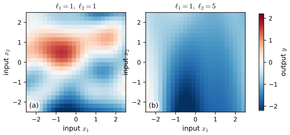
fig_18_2. Reproduces Murphy (2023), Figure 18.2. Download: PDF · SVG18.2.1.3 Matérn kernels
p. 685, (18.13)–(18.16) The SE kernel gives very smooth functions. The Matérn kernel, \[ K(r;\nu,\ell)=\frac{2^{1-\nu}}{\Gamma(\nu)}\Big(\frac{\sqrt{2\nu}\,r}{\ell}\Big)^{\nu}K_\nu\Big(\frac{\sqrt{2\nu}\,r}{\ell}\Big),\tag{18.13} \] with \(K_\nu\) the modified Bessel function of the second kind, allows rougher functions. For half-integer \(\nu\) it is an exponential times a polynomial: \[ K(r;\tfrac12)=e^{-r/\ell},\quad K(r;\tfrac32)=\Big(1+\tfrac{\sqrt3r}{\ell}\Big)e^{-\sqrt3r/\ell},\quad K(r;\tfrac52)=\Big(1+\tfrac{\sqrt5r}{\ell}+\tfrac{5r^2}{3\ell^2}\Big)e^{-\sqrt5r/\ell}.\tag{18.14--18.16} \] The smoothness is controlled by \(\nu\): the sample functions are \(k\) times (mean-square) differentiable iff \(\nu>k\), and \(\nu\to\infty\) gives the SE kernel. This is visible in the small-\(r\) behaviour: \(1-K(r;\tfrac12)\approx r/\ell\) is not smooth at 0 (continuous but nowhere differentiable paths, the Ornstein–Uhlenbeck process), whereas \((1+s)e^{-s}=1-\tfrac{s^2}2+\tfrac{s^3}3-\cdots\) with \(s=\sqrt3r/\ell\) is twice differentiable at 0 (once-differentiable paths). In Section 18.2.1.6 the smoothness is explained by the heavy tail of the spectral density. Figures 18.3 and 18.4 show the kernels \(K(x,0)\) and samples for twelve kernels.
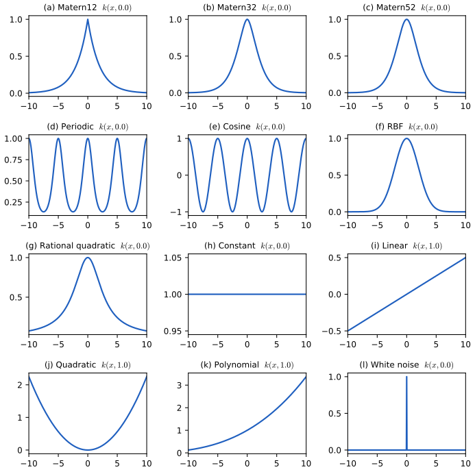
fig_18_3. Reproduces Murphy (2023), Figure 18.3. Download: PDF · SVG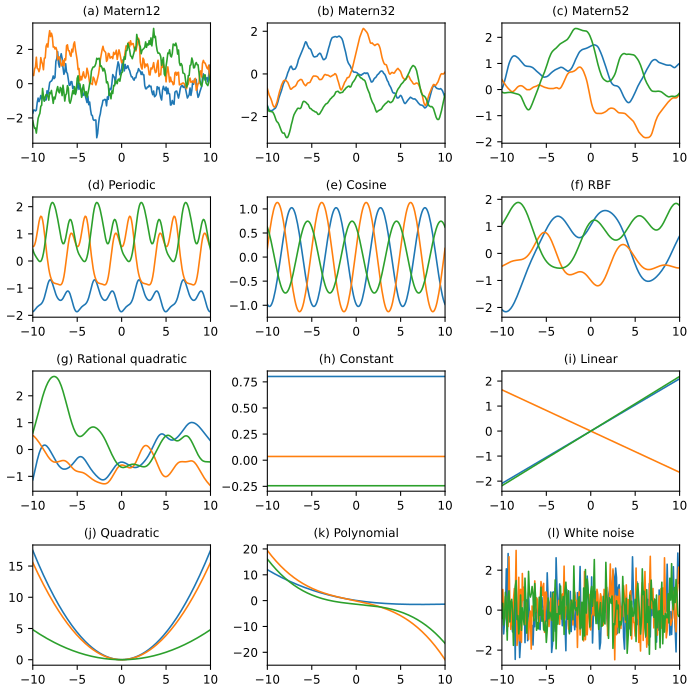
fig_18_4. Reproduces Murphy (2023), Figure 18.4. Download: PDF · SVG18.2.1.4 Periodic kernels
p. 687, (18.17)–(18.19) A periodic random function is obtained by mapping \(x\) to the circle \(\bm u(x)=(\cos x,\sin x)\) and using an SE kernel there; since \((\cos x-\cos x')^2+(\sin x-\sin x')^2=4\sin^2\!\big(\tfrac{x-x'}2\big)\), \[ K(x,x')=\exp\!\Big(-\frac{2\sin^2((x-x')/2)}{\ell^2}\Big),\qquad K_{\rm per}(r;\ell,p)=\exp\!\Big(-\frac{2}{\ell^2}\sin^2\!\big(\tfrac{\pi r}{p}\big)\Big),\qquad K(r;p)=\cos\!\big(\tfrac{2\pi r}{p}\big).\tag{18.17--18.19} \] The middle one (exp-sine-squared) has period \(p\); the last (cosine) is a degenerate kernel of rank 2, \(\cos(2\pi x/p)\cos(2\pi x'/p)+\sin(2\pi x/p)\sin(2\pi x'/p)\).
18.2.1.5 Rational quadratic kernel
p. 688, (18.20)–(18.21) \(K_{\rm RQ}(r;\ell,\alpha)=(1+r^2/(2\alpha\ell^2))^{-\alpha}\) is proportional to a Student density; it is a scale mixture of SE kernels with different length scales, and \(\alpha\to\infty\) gives the SE kernel.
Filling the gap 18.1: the rational quadratic kernel is a gamma mixture of SE kernels p. 688, (18.21)
Derivation
Write the SE kernel in terms of the precision \(\tau=1/\ell'^2\): \(K_{\rm SE}(r\given\tau)=e^{-\tau r^2/2}\). Let \(\tau\sim\mathrm{Ga}(\alpha,\beta)\) with shape \(\alpha\) and rate \(\beta\), density \(\beta^\alpha\tau^{\alpha-1}e^{-\beta\tau}/\Gamma(\alpha)\). Then \[ \int_0^\infty\frac{\beta^\alpha\tau^{\alpha-1}}{\Gamma(\alpha)}e^{-\beta\tau}e^{-\tau r^2/2}\,\d\tau=\frac{\beta^\alpha}{(\beta+r^2/2)^\alpha}=\Big(1+\frac{r^2}{2\beta}\Big)^{-\alpha},\] because the integrand is an unnormalised \(\mathrm{Ga}(\alpha,\beta+r^2/2)\) density. Choosing \(\beta=\alpha\ell^2\) gives exactly \(K_{\rm RQ}(r;\ell,\alpha)\) (18.20); the mean of \(\tau\) is then \(\alpha/\beta=1/\ell^2\), so \(\ell\) is the length scale of the average SE component. (The book writes \(\mathrm{Ga}(\alpha,\ell^2)\); the rate must be \(\alpha\ell^2\), see the notes on the book.) As \(\alpha\to\infty\), \((1+x/\alpha)^{-\alpha}\to e^{-x}\) with \(x=r^2/2\ell^2\), so \(K_{\rm RQ}\to K_{\rm SE}\); the gamma law concentrates at \(1/\ell^2\). A mixture of positive definite kernels with non-negative weights is positive definite (Gap 18.4), so the RQ kernel is valid, and its sample paths are infinitely differentiable like those of the SE kernel but have variation at many scales. Confirmed numerically by quadrature for several \((\alpha,\ell,r)\).
18.2.1.6 Kernels from spectral densities
p. 688, (18.22) For a stationary kernel \(K(\bm\delta)\), \(\bm\delta=\bm x-\bm x'\), Bochner's theorem says that it is positive definite if and only if it is the Fourier transform of a finite non-negative measure, the spectral density \(p(\bm\omega)\): \[ K(\bm\delta)=\int_{\R^d}p(\bm\omega)\,e^{2\pi j\bm\omega^\T\bm\delta}\,\d\bm\omega .\tag{18.22} \] (The book writes \(e^{j\bm\omega^\T\bm\delta}\); the two conventions differ by the factor \(2\pi\) in \(\bm\omega\) and I use the ordinary-frequency one, which also makes the spectral mixture kernel (18.172) correct.) The SE kernel has a Gaussian spectral density with bandwidth inversely proportional to \(\ell\): a long length scale means low frequencies. Since a Gaussian has light tails, the SE kernel gives almost no weight to high frequencies. A Student-\(t\) spectral density has heavy tails and gives the Matérn kernel, and a scale-location mixture of Gaussians gives the spectral mixture kernel of Section 18.6.5.
Filling the gap 18.2: spectral densities of the SE, Matérn and spectral mixture kernels pp. 688, 725, (18.22), (18.172)
Derivation
Bochner's theorem (one direction, and why). If \(K(\bm\delta)=\int e^{2\pi j\bm\omega^\T\bm\delta}\d\mu(\bm\omega)\) with \(\mu\ge0\), then for any points and coefficients \(\sum_{m,n}c_m\bar c_nK(\bm x_m-\bm x_n)=\int|\sum_mc_me^{2\pi j\bm\omega^\T\bm x_m}|^2\d\mu\ge0\), so \(K\) is positive definite. The converse (every continuous positive definite \(K\) arises this way) is Bochner's theorem and is quoted. The kernel is real and even, so \(\mu\) is symmetric and \(K(\bm\delta)=\int p(\bm\omega)\cos(2\pi\bm\omega^\T\bm\delta)\d\bm\omega\).
SE. In one dimension the Fourier transform of a Gaussian is a Gaussian: \(\int e^{-\delta^2/2\ell^2}e^{-2\pi j\omega\delta}\d\delta=\sqrt{2\pi}\,\ell\,e^{-2\pi^2\ell^2\omega^2}\). By Fourier inversion, \[ p_{\rm SE}(\omega)=\sqrt{2\pi}\,\ell\,e^{-2\pi^2\ell^2\omega^2},\qquad \int p_{\rm SE}=K(0)=1 .\] This is exactly the \(\N(0,(2\pi\ell)^{-2})\) density: the frequency has standard deviation \(1/(2\pi\ell)\), inversely proportional to \(\ell\) as the text says. (The book prints the factor \(\ell^2\) instead of \(\ell\); then the density integrates to \(\ell\), not to \(K(0)=1\).) In \(d\) dimensions the density is \((2\pi)^{d/2}\ell^d e^{-2\pi^2\ell^2\|\bm\omega\|^2}\).
Matérn as a scale mixture of SE kernels, hence a Student-\(t\) spectrum. Let \(u\sim\chi^2_{2\nu}\) (density \(u^{\nu-1}e^{-u/2}/(2^\nu\Gamma(\nu))\)) and consider the Gaussian scale mixture \(\omega=s\,z\sqrt{2\nu/u}\) with \(z\sim\N(0,1)\) independent, \(s=1/(2\pi\ell)\). This is exactly a Student-\(t\) variable with \(2\nu\) degrees of freedom and scale \(s\) (density \(\propto(1+\omega^2/(2\nu s^2))^{-(\nu+1/2)}\propto(2\nu/\ell^2+4\pi^2\omega^2)^{-(\nu+1/2)}\)). Its characteristic function is \[ K(\delta)=\E\,e^{2\pi j\omega\delta}=\E_u\exp\!\big(-\tfrac12(2\pi\delta s)^2\tfrac{2\nu}{u}\big)=\E_u\exp\!\Big(-\frac{\nu\delta^2}{\ell^2u}\Big)=\int_0^\infty\frac{u^{\nu-1}e^{-u/2-a/u}}{2^\nu\Gamma(\nu)}\d u,\quad a=\frac{\nu\delta^2}{\ell^2}.\] Using \(\int_0^\infty u^{\nu-1}e^{-bu-a/u}\d u=2(a/b)^{\nu/2}K_\nu(2\sqrt{ab})\) with \(b=\tfrac12\), the integral equals \(\dfrac{2(2a)^{\nu/2}K_\nu(\sqrt{2a})}{2^\nu\Gamma(\nu)}=\dfrac{2^{1-\nu}}{\Gamma(\nu)}z^\nu K_\nu(z)\) with \(z=\sqrt{2\nu}\,\delta/\ell\): this is the Matérn kernel (18.13) exactly. So the Matérn kernel has spectral density \(\propto(2\nu/\ell^2+4\pi^2\omega^2)^{-(\nu+1/2)}\), a Student-\(t\) with \(2\nu\) degrees of freedom; in \(d\) dimensions the exponent is \(-(\nu+d/2)\). This also proves positive definiteness. Smaller \(\nu\) means heavier tails, more high-frequency power and rougher paths; \(\nu\to\infty\) turns the Student law into the Gaussian of the SE kernel. I checked numerically that the Fourier transform of (18.13) is proportional to this expression (constant ratio to four digits).
Spectral mixture. Take the symmetric Gaussian mixture \(p(\omega)=\sum_iw_i\tfrac12[\N(\omega\given\mu_i,v_i)+\N(\omega\given-\mu_i,v_i)]\). The characteristic function of \(\N(\mu,v)\) is \(e^{2\pi j\mu\delta-2\pi^2v\delta^2}\); symmetrising the real part gives \[ K(\delta)=\sum_iw_i\cos(2\pi\mu_i\delta)\,e^{-2\pi^2v_i\delta^2},\tag{18.172} \] the spectral mixture kernel. Each term is the product of a cosine (a periodic part at frequency \(\mu_i\)) and an SE kernel with length scale \(\ell_i=1/(2\pi\sqrt{v_i})\) (a decay of the periodicity). Because scale-location mixtures of Gaussians are dense among densities, the family can approximate any stationary kernel.
18.2.2 Nonstationary kernels
p. 689 A stationary kernel treats every location alike. A nonstationary kernel lets correlations change with location, useful for environmental data.
18.2.2.1 Polynomial kernels
p. 689, (18.23)–(18.26) The homogeneous polynomial kernel \(K(\bm x,\bm x')=(\bm x^\T\bm x')^M\) contains all monomials of order \(M\); for \(M=2\) in 2-d, \((\bm x^\T\bm x')^2=(x_1x_1')^2+(x_2x_2')^2+2(x_1x_1')(x_2x_2')\) is an inner product of the three features \((x_1^2,\sqrt2x_1x_2,x_2^2)\) (18.24). The inhomogeneous version \((\bm x^\T\bm x'+c)^M\) (18.25) contains all monomials up to degree \(M\); the expansion for \(M=2\), \(c=1\) (18.26) has six distinct terms (the book's display has a slip: it lists \(x_2x_2\) where \(x_2x_2'\) is meant).
18.2.2.2 Gibbs kernel
p. 689, (18.27) Let the length scale and the amplitude of an RBF kernel depend on the input: \[ K(\bm x,\bm x')=\sigma(\bm x)\sigma(\bm x')\sqrt{\frac{2\ell(\bm x)\ell(\bm x')}{\ell(\bm x)^2+\ell(\bm x')^2}}\exp\!\Big(-\frac{\|\bm x-\bm x'\|^2}{\ell(\bm x)^2+\ell(\bm x')^2}\Big).\tag{18.27} \] For constant \(\ell\) and \(\sigma\) it reduces to the usual SE kernel (the prefactor is \(1\) and the exponent \(-r^2/2\ell^2\)). The functions \(\ell(\cdot),\sigma(\cdot)\) can themselves be modelled by a GP.
Filling the gap 18.3: the Gibbs kernel is positive definite p. 689, (18.27)
Derivation
The book states the kernel without checking that it is valid. In one dimension (the general case is the same with powers of \(d/2\) in the prefactor) put \(g_x(u)=(2/\pi\ell(x)^2)^{1/4}\exp(-(x-u)^2/\ell(x)^2)\). A Gaussian integral gives \[ \int g_x(u)g_{x'}(u)\,\d u=\Big(\frac2\pi\Big)^{1/2}(\ell\ell')^{-1/2}\sqrt{\frac{\pi\ell^2\ell'^2}{\ell^2+\ell'^2}}\,e^{-(x-x')^2/(\ell^2+\ell'^2)}=\sqrt{\frac{2\ell\ell'}{\ell^2+\ell'^2}}\,e^{-(x-x')^2/(\ell^2+\ell'^2)},\] with \(\ell=\ell(x),\ell'=\ell(x')\). So the Gibbs kernel is \(\sigma(x)\sigma(x')\langle g_x,g_{x'}\rangle_{L^2}\): the Gram matrix of vectors in the Hilbert space \(L^2\), scaled by \(\sigma(x)\sigma(x')\). Every such matrix is positive semi-definite (\(\sum c_ic_j\langle g_i,g_j\rangle=\|\sum c_ig_i\|^2\ge0\)). The kernel is a "convolution kernel": a smoothing of white noise by a Gaussian window whose width varies with location. Confirmed numerically (smallest Gram eigenvalue \(\ge0\) for random \(\ell(x),\sigma(x)\), and equality with the SE kernel for constant \(\ell\)).
18.2.2.3 Other non-stationary kernels
p. 689 Other routes are the neural network kernel (Section 18.7.1), non-stationary spectral kernels and deep GPs (Section 18.7.3).
18.2.3 Kernels for nonvectorial (structured) inputs
p. 690 Kernels are convenient when inputs are strings or graphs, which are hard to featurise. A string kernel counts shared \(n\)-grams; the random-walk graph kernel counts the paths produced by simultaneous random walks on two graphs. The point is that only a positive definite similarity is needed, not a vector representation.
18.2.4 Making new kernels from old
p. 690, (18.28)–(18.36) If \(K_1,K_2\) are kernels then so are \(cK_1\) (\(c>0\)), \(f(\bm x)K_1(\bm x,\bm x')f(\bm x')\) for any function \(f\), \(q(K_1)\) for a polynomial \(q\) with non-negative coefficients, \(\exp(K_1)\), \(\bm x^\T\bm A\bm x'\) for \(\bm A\) positive semi-definite, and the sum \(K_1+K_2\) (18.35) and product \(K_1K_2\) (18.36). Starting from the linear kernel one gets the polynomial kernels, and from (18.34), \(\exp(-\|\bm x-\bm x'\|^2/2\sigma^2)=e^{-\|\bm x\|^2/2\sigma^2}e^{\bm x^\T\bm x'/\sigma^2}e^{-\|\bm x'\|^2/2\sigma^2}\), the validity of the SE kernel. A product yields a conjunction of the properties of the factors (Figure 18.5); a sum yields a disjunction (Figure 18.6).
Filling the gap 18.4: closure of the Mercer kernels, including the product rule pp. 690–691, (18.28)–(18.36)
Derivation
Let \(\bm A=(K_1(\bm x_i,\bm x_j))\) and \(\bm B=(K_2(\bm x_i,\bm x_j))\) be positive semi-definite Gram matrices and \(\bm c\in\R^N\).
- Scaling, sum, \(fKf\), \(\bm x^\T\bm A\bm x'\). \(\bm c^\T(\alpha\bm A)\bm c=\alpha\bm c^\T\bm A\bm c\ge0\); \(\bm c^\T(\bm A+\bm B)\bm c\ge0\) trivially; for \(f\) a function, \(\sum_{ij}c_ic_jf_iK_1(\bm x_i,\bm x_j)f_j=\sum_{ij}(c_if_i)(c_jf_j)K_1\ge0\); and \(\bm x^\T\bm A\bm x'=(\bm A^{1/2}\bm x)^\T(\bm A^{1/2}\bm x')\) is an inner product of feature vectors.
- Product (Schur product theorem). Write \(\bm B=\sum_k\lambda_k\bm u_k\bm u_k^\T\) with \(\lambda_k\ge0\). The entry-wise (Hadamard) product is \(\bm A\circ\bm B=\sum_k\lambda_k\,\diag(\bm u_k)\,\bm A\,\diag(\bm u_k)\), because \((\bm A\circ\bm u\bm u^\T)_{ij}=u_iA_{ij}u_j\). Each term is a congruence of a PSD matrix, hence PSD, and a non-negative combination of PSD matrices is PSD. Probabilistic reading: if \(f_1\sim\GP(0,K_1)\) and \(f_2\sim\GP(0,K_2)\) are independent, \(f_1(\bm x)f_2(\bm x)\) has covariance \(\E[f_1f_1']\E[f_2f_2']=K_1K_2\), which is why the product keeps both properties.
- Polynomials and exponential. Powers \(K_1^m\) are repeated products; \(q(K_1)\) with non-negative coefficients (constants are kernels \(c\ge0\)) is a sum of such terms. The set of PSD matrices is closed under limits, so \(\exp(K_1)=\sum_mK_1^m/m!\) is a kernel.
- The SE kernel. \(K_1=\exp(\bm x^\T\bm x'/\sigma^2)\) is a kernel by the exponential rule applied to the linear kernel, and (18.34) is of the form \(f(\bm x)K_1f(\bm x')\) with \(f=e^{-\|\bm x\|^2/2\sigma^2}\). (It is even strictly positive definite on distinct points, since its spectral density is positive everywhere.)
Numerically: Gram matrices of \(K_{\rm SE}+K_{\rm per}\), \(K_{\rm SE}K_{\rm per}\), \(K_{\rm lin}K_{\rm SE}\), \(\exp K_{\rm SE}\), \((2+K_{\rm lin})^3\), \(f K f\) and a triple product all have smallest eigenvalue \(\ge-10^{-9}\), whereas \(-K_{\rm SE}\) does not. Not every operation preserves positive definiteness: \(K_1-K_2\) and \(\exp(-K_1)\) need not be kernels.
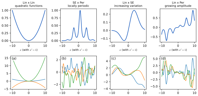
fig_18_5. Reproduces Murphy (2023), Figure 18.5. Download: PDF · SVG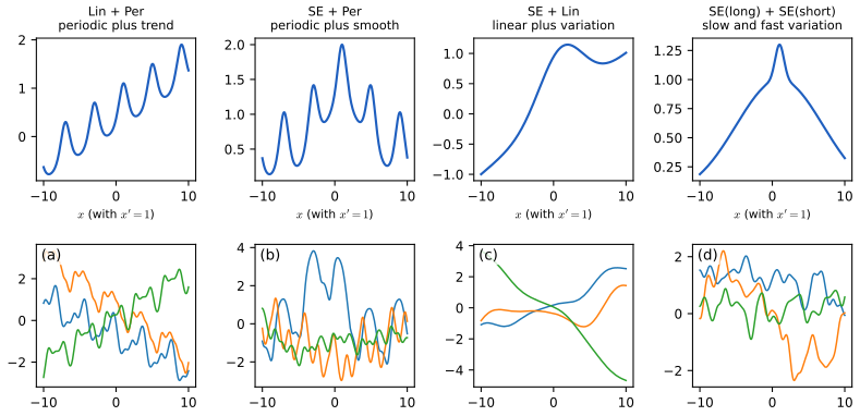
fig_18_6. Reproduces Murphy (2023), Figure 18.6. Download: PDF · SVGSee also: Bayesian and Probabilistic ML, 6.2 constructing kernels; Introduction volume, 17.1.2 some popular Mercer kernels. Section 18.8.1 combines kernels to forecast a time series.
18.2.5 Mercer's theorem
pp. 691–692, (18.37)–(18.41) A positive semi-definite matrix has an eigendecomposition \(\bm K=\bm U\bm\Lambda\bm U^\T\) with \(\lambda_m\ge0\), so \(k_{ij}=\sum_m\lambda_m\phi_m(\bm x_i)\phi_m(\bm x_j)\) with \(\phi_m(\bm x_i)=U_{im}\): the Gram matrix is an inner product of (implicitly defined) feature vectors (18.37)–(18.38). (The book writes the decomposition as \(\bm U^\T\bm\Lambda\bm U\) with eigenvectors in columns of \(\bm U\); the \(\bm U\bm\Lambda\bm U^\T\) convention is used here.) For a kernel function the analogue uses eigenfunctions with respect to a measure \(\mu\), \[ \int K(\bm x,\bm x')\phi(\bm x)\,\d\mu(\bm x)=\lambda\phi(\bm x'),\qquad\int\phi_i\phi_j\,\d\mu=\delta_{ij},\qquad K(\bm x,\bm x')=\sum_{m=1}^\infty\lambda_m\phi_m(\bm x)\phi_m(\bm x'), \tag{18.39--18.41} \] the last being Mercer's theorem. A degenerate kernel has finitely many non-zero eigenvalues; for the quadratic kernel \(\langle\bm x,\bm x'\rangle^2=\bm\phi(\bm x)^\T\bm\phi(\bm x')\) with \(\bm\phi=(x_1^2,\sqrt2x_1x_2,x_2^2)\), so the Gram matrix has rank at most 3. The SE kernel has infinitely many features. Replacing \(\bm\phi(\bm x)^\T\bm\phi(\bm x')\) by \(K(\bm x,\bm x')\) is the kernel trick.
Filling the gap 18.5: Mercer's theorem, the finite version, and the SE eigenvalues pp. 691–692
Derivation
Finite version. By the spectral theorem a symmetric PSD \(\bm K\) equals \(\sum_m\lambda_m\bm u_m\bm u_m^\T\) with orthonormal \(\bm u_m\) and \(\lambda_m\ge0\). With \(\bm\psi(\bm x_i)=(\sqrt{\lambda_m}U_{im})_m\), \(k_{ij}=\bm\psi(\bm x_i)^\T\bm\psi(\bm x_j)\). The features are not unique (any orthogonal rotation gives another), only the inner products are.
Function version. For a continuous kernel on a compact set with a finite measure \(\mu\), the integral operator \((T_Kf)(\bm x')=\int K(\bm x,\bm x')f(\bm x)\d\mu(\bm x)\) is compact, self-adjoint and, for a positive definite kernel, positive. The spectral theorem for compact self-adjoint operators gives orthonormal eigenfunctions \(\phi_m\) with eigenvalues \(\lambda_m\ge0\to0\), and Mercer's theorem states that the series (18.41) converges absolutely and uniformly. The proof is quoted (it is in the first volume: 17.1.1); what matters for the rest of the chapter is the meaning of the eigenvalues, which set the amount of variance carried by each feature.
A closed form worth knowing. For the SE kernel with length scale \(\ell\) and the Gaussian measure \(\mu=\N(0,s^2)\), with \(a=1/(4s^2)\), \(b=1/(2\ell^2)\), \(c=\sqrt{a^2+2ab}\), \(A=a+b+c\), \(B=b/A\), the eigenvalues are \(\lambda_k=\sqrt{2a/A}\,B^k\), \(k=0,1,\dots\) (Zhu et al., 1998; Rasmussen and Williams, Section 4.3.1): they decay geometrically, so a few features carry almost all the variance and the Gram matrix is numerically low rank. I confirmed the first six against Gauss–Hermite quadrature of the integral operator (agreement to \(10^{-6}\)). The geometric decay is what makes Nyström and inducing-point approximations (Section 18.5) work for smooth kernels, and why the Matérn kernel with its power-law decay is harder to compress.
18.2.6 Approximating kernels with random features
pp. 692–693, (18.42)–(18.43) Kernel methods cost \(O(N^3)\) because of the inversion of the Gram matrix. For shift-invariant kernels one can instead approximate the feature map by \(D\) random cosines, reducing the cost to \(O(ND^2+D^3)\). By Bochner (18.22) the SE kernel is an expectation over a Gaussian frequency distribution, so a Monte Carlo average over frequencies \(\bm z_j\sim\N(\bm 0,\ell^{-2}\bm I)\) gives \(K(\bm x,\bm x')\approx\bm\phi(\bm x)^\T\bm\phi(\bm x')\) with \[ \bm\phi(\bm x)=\sqrt{\tfrac1D}\big[\sin(\bm Z^\T\bm x),\cos(\bm Z^\T\bm x)\big],\qquad\bm Z=\tfrac1\ell\bm G,\ G_{ij}\sim\N(0,1). \tag{18.42--18.43} \] These are random Fourier features (random kitchen sinks); orthogonal random features reduce the variance further. The model \(f(\bm x)=\bm W\bm\phi(\bm Z\bm x)+\bm b\) is a one-hidden-layer network with fixed random input weights and trained output weights, a linear model with cost \(O(N)\) per pass. Too few features lose expressive power.
Filling the gap 18.6: random Fourier features: unbiasedness, variance and the \(D^{-1/2}\) rate pp. 692–693, (18.42)
Derivation
Let \(\bm\delta=\bm x-\bm x'\) and \(\bm z_1,\dots,\bm z_D\) iid \(\N(\bm 0,\ell^{-2}\bm I)\). Since \(\sin a\sin b+\cos a\cos b=\cos(a-b)\), \[ \bm\phi(\bm x)^\T\bm\phi(\bm x')=\frac1D\sum_{j=1}^D\cos(\bm z_j^\T\bm\delta)=:\hat K(\bm\delta).\] Unbiased. \(\E\cos(\bm z^\T\bm\delta)=\mathrm{Re}\,\E e^{j\bm z^\T\bm\delta}=\mathrm{Re}\,e^{-\|\bm\delta\|^2/2\ell^2}=K_{\rm SE}(\bm\delta)\), the characteristic function of the Gaussian. (The book's "\(\bm\phi(\bm x)^\T\bm\phi(\bm x)\)" should read \(\bm\phi(\bm x)^\T\bm\phi(\bm x')\).) Variance. The summands are iid, and \(\E\cos^2(\bm z^\T\bm\delta)=\tfrac12(1+\E\cos(2\bm z^\T\bm\delta))=\tfrac12(1+K^4)\) because \(K(2\bm\delta)=e^{-4\|\bm\delta\|^2/2\ell^2}=K^4\). Hence \[ \var[\hat K(\bm\delta)]=\frac1D\Big[\frac{1+K^4}2-K^2\Big]=\frac{(1-K^2)^2}{2D}, \qquad K=K_{\rm SE}(\bm\delta). \] The error is zero at \(\bm\delta=\bm0\) (where \(K=1\)) and for large \(\|\bm\delta\|\) it is of order \(1/\sqrt{2D}\) in absolute terms while \(K\to0\): random features approximate the tails worst in relative terms. The standard deviation is \(O(D^{-1/2})\); Rahimi and Recht (2008) show that the uniform error over a compact set is also \(O(D^{-1/2})\) up to logarithms, with probability bounds of the form \(2^8(\sigma_pR/\varepsilon)^2\exp(-D\varepsilon^2/(4(d+2)))\) (quoted). In Figure 18.S1 the rms error falls by a factor of \(4.2\) when \(D\) goes from 16 to 256 (a factor \(4\) is expected), and the sample variance of 4000 draws at \(D=20\) matches \((1-K^2)^2/40\) to 1%.
As a GP. The finite model \(f=\bm w^\T\bm\phi\), \(\bm w\sim\N(\bm 0,\bm I)\), is a degenerate GP with kernel \(\hat K\): Bayesian linear regression (Section 18.3.3) in \(2D\) features, with cost \(O(ND^2+D^3)\), which approaches the exact GP as \(D\to\infty\).
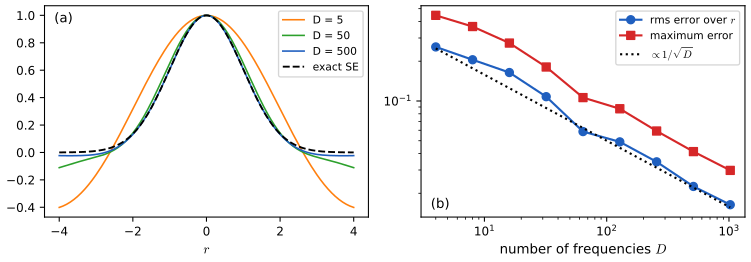
fig_S18_1. Download: PDF · SVG18.3 GPs with Gaussian likelihoods
p. 693 With a Gaussian likelihood every computation is linear algebra. The basics (noise-free and noisy prediction, weight space against function space, numerical issues) are in the first volume, 17.2 and Bayesian and Probabilistic ML, 6.4; below they are stated, and the complete arguments are given where the book leaves steps out.
18.3.1 Predictions using noise-free observations
pp. 693–694, (18.44)–(18.47) Suppose \(y_n=f(\bm x_n)\) exactly. For test inputs \(\bm X_*\) the joint prior of training and test function values is Gaussian, \[ \begin{pmatrix}\bm f_X\\\bm f_*\end{pmatrix}\sim\N\!\left(\begin{pmatrix}\bm\mu_X\\\bm\mu_*\end{pmatrix},\begin{pmatrix}\bm K_{X,X}&\bm K_{X,*}\\\bm K_{X,*}^\T&\bm K_{*,*}\end{pmatrix}\right),\tag{18.44}\] and Gaussian conditioning (Section 2.3.1) gives \(p(\bm f_*\given\bm X_*,\mathcal D)=\N(\bm\mu_{*|X},\bm\Sigma_{*|X})\) with \[ \bm\mu_{*|X}=\bm\mu_*+\bm K_{X,*}^\T\bm K_{X,X}^{-1}(\bm f_X-\bm\mu_X),\qquad\bm\Sigma_{*|X}=\bm K_{*,*}-\bm K_{X,*}^\T\bm K_{X,X}^{-1}\bm K_{X,*}. \tag{18.45--18.47} \] The posterior interpolates the data with no uncertainty at the observed inputs, and the uncertainty grows away from them (Figure 18.7, left and middle). Drawing a sample on \(N_*\) points by a Cholesky factor costs \(O(N_*^3)\); pathwise methods reduce this to \(O(N_*)\).
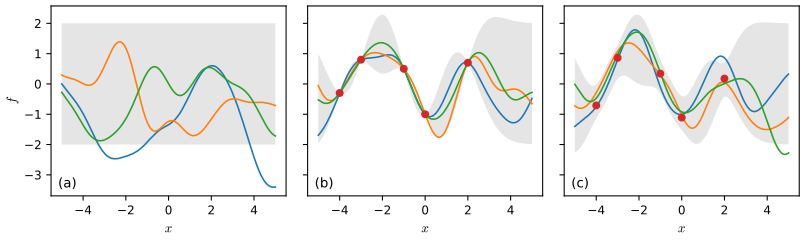
fig_18_7. Reproduces Murphy (2023), Figure 18.7. Download: PDF · SVG18.3.2 Predictions using noisy observations
pp. 694–695, (18.48)–(18.57) With \(y_n=f(\bm x_n)+\epsilon_n\), \(\epsilon_n\sim\N(0,\sigma_y^2)\), the observed responses have covariance \(\bm K_{X,X}+\sigma_y^2\bm I_N\) (18.48)–(18.49), and the joint of \((\bm y,\bm f_*)\) is (18.50) with \(\bm K_{X,X}\) replaced by \(\bm K_\sigma=\bm K_{X,X}+\sigma_y^2\bm I\). Conditioning gives \[ \bm\mu_{*|X}=\bm\mu_*+\bm K_{X,*}^\T\bm K_\sigma^{-1}(\bm y-\bm\mu_X),\qquad\bm\Sigma_{*|X}=\bm K_{*,*}-\bm K_{X,*}^\T\bm K_\sigma^{-1}\bm K_{X,*}\tag{18.52--18.53} \] (the book writes the covariance of the joint in (18.50) with \(\bm K_{X,X}+\sigma_y^2\bm I\) in the first block). For a zero mean, the posterior mean at one input is a weighted sum of kernels centred on the data, \[ \mu_{*|X}=\bm k_*^\T\bm K_\sigma^{-1}\bm y=\sum_{n=1}^NK(\bm x_*,\bm x_n)\alpha_n,\qquad\bm\alpha=\bm K_\sigma^{-1}\bm y,\tag{18.55--18.57} \] so fitting means computing \(\bm\alpha\); afterwards the mean costs \(O(N)\) and the variance \(O(N^2)\) per test point.
Filling the gap 18.7: the posterior is a GP; the Cholesky formulas; interpolation pp. 693–698, (18.45)–(18.57), (18.75)–(18.77)
Derivation
The posterior is again a GP. For any finite test set the posterior is the Gaussian conditional (18.52)–(18.53). These Gaussians are consistent under marginalisation (the marginal of the conditional on a subset of the test points is the conditional for that subset), so by Kolmogorov's theorem they define a GP, \[ f\given\mathcal D\sim\GP\big(m_{\rm post},K_{\rm post}\big),\quad m_{\rm post}(\bm x)=m(\bm x)+\bm k_{\bm x}^\T\bm K_\sigma^{-1}(\bm y-\bm\mu_X),\quad K_{\rm post}(\bm x,\bm x')=K(\bm x,\bm x')-\bm k_{\bm x}^\T\bm K_\sigma^{-1}\bm k_{\bm x'}, \] with \(\bm k_{\bm x}=(K(\bm x,\bm x_n))_n\). The posterior covariance is the prior covariance minus a positive semi-definite correction (\(\bm K_\sigma\succ0\)), so data can only reduce uncertainty. The predictive distribution of a new noisy observation adds \(\sigma_y^2\) to the variance.
Interpolation. If the noise is zero, take \(\bm X_*=\bm X\): \(\bm\mu_{*|X}=\bm K\bm K^{-1}\bm f_X=\bm f_X\) and \(\bm\Sigma_{*|X}=\bm K-\bm K\bm K^{-1}\bm K=\bm 0\). With noise \(\sigma_y^2>0\) the posterior mean at a training input is \(\bm K\bm K_\sigma^{-1}\bm y\ne\bm y\): it shrinks the data towards the smooth fit.
Stable computation. Do not invert \(\bm K_\sigma\). Its Cholesky factor \(\bm K_\sigma=\bm L\bm L^\T\) costs \(O(N^3)\) once. Then \(\bm\alpha=\bm L^{-\T}(\bm L^{-1}\bm y)\) by two triangular solves (18.75) and \(\mu_*=\bm k_*^\T\bm\alpha\). For the variance, \(\bm k_*^\T\bm K_\sigma^{-1}\bm k_*=\|\bm L^{-1}\bm k_*\|^2=\bm v^\T\bm v\) with \(\bm v=\bm L\backslash\bm k_*\), so \(\sigma_*^2=k_{**}-\bm v^\T\bm v\) (18.76), \(O(N^2)\) per test point. Since the determinant of a triangular matrix is the product of its diagonal, \(\log|\bm K_\sigma|=2\sum_n\log L_{nn}\), and the marginal likelihood (18.74) becomes \[ \log p(\bm y\given\bm X)=-\tfrac12\bm y^\T\bm\alpha-\sum_{n=1}^N\log L_{nn}-\tfrac N2\log2\pi.\tag{18.77} \] I checked that the Cholesky implementation reproduces brute-force conditioning of the joint (18.50) (mean, full covariance, diagonal), that (18.77) equals the multivariate normal log density, and that the noise-free GP interpolates with zero variance.
See also: Introduction volume, 17.2.5 numerical issues.
18.3.3 Weight space vs function space
pp. 695–696, (18.58)–(18.63) Bayesian linear regression \(y=\bm w^\T\bm\phi(\bm x)+\epsilon\) with prior \(\bm w\sim\N(\bm 0,\bm\Sigma_w)\) has posterior \(\N(\sigma_y^{-2}\bm A^{-1}\bm\Phi^\T\bm y,\bm A^{-1})\) with \(\bm A=\sigma_y^{-2}\bm\Phi^\T\bm\Phi+\bm\Sigma_w^{-1}\) (18.58)–(18.59) and predictive \(\N(\sigma_y^{-2}\bm\phi_*^\T\bm A^{-1}\bm\Phi^\T\bm y,\ \bm\phi_*^\T\bm A^{-1}\bm\phi_*)\) (18.60). This equals GP regression with the kernel \(K(\bm x,\bm x')=\bm\phi(\bm x)^\T\bm\Sigma_w\bm\phi(\bm x')\): with \(\bm K=\bm\Phi\bm\Sigma_w\bm\Phi^\T\), \(\bm k_*=\bm\Phi\bm\Sigma_w\bm\phi_*\), \(k_{**}=\bm\phi_*^\T\bm\Sigma_w\bm\phi_*\), both give (18.61)–(18.63). A GP works in function space and may use kernels with infinitely many features; a non-zero mean is a constant feature.
Filling the gap 18.8: weight space and function space agree pp. 695–696, (18.60)–(18.63)
Derivation
The book invokes the matrix inversion lemma; here is the short route. Let \(\bm K=\bm\Phi\bm\Sigma_w\bm\Phi^\T\) and \(\bm A=\sigma_y^{-2}\bm\Phi^\T\bm\Phi+\bm\Sigma_w^{-1}\). Then \[ \bm A\,\bm\Sigma_w\bm\Phi^\T=\sigma_y^{-2}\bm\Phi^\T\bm\Phi\bm\Sigma_w\bm\Phi^\T+\bm\Phi^\T=\sigma_y^{-2}\bm\Phi^\T(\bm K+\sigma_y^2\bm I)\quad\Longrightarrow\quad\bm\Sigma_w\bm\Phi^\T(\bm K+\sigma_y^2\bm I)^{-1}=\sigma_y^{-2}\bm A^{-1}\bm\Phi^\T. \] (Push-through identity.) Multiplying by \(\bm\phi_*^\T\) on the left and \(\bm y\) on the right gives the means: \(\sigma_y^{-2}\bm\phi_*^\T\bm A^{-1}\bm\Phi^\T\bm y=\bm k_*^\T(\bm K+\sigma_y^2\bm I)^{-1}\bm y\) (18.62). For the variance, from \(\bm A^{-1}\bm\Sigma_w^{-1}=\bm I-\sigma_y^{-2}\bm A^{-1}\bm\Phi^\T\bm\Phi\), \[ \bm A^{-1}=\bm\Sigma_w-\sigma_y^{-2}\bm A^{-1}\bm\Phi^\T\bm\Phi\bm\Sigma_w=\bm\Sigma_w-\bm\Sigma_w\bm\Phi^\T(\bm K+\sigma_y^2\bm I)^{-1}\bm\Phi\bm\Sigma_w,\] and \(\bm\phi_*^\T\bm A^{-1}\bm\phi_*=k_{**}-\bm k_*^\T(\bm K+\sigma_y^2\bm I)^{-1}\bm k_*\) (18.63). (The book prints \(\sigma_y\bm I\) in (18.62); the correct term is \(\sigma_y^2\bm I\).) Cost: the weight-space form inverts a \(D\times D\) matrix (\(D\) features), the function-space form an \(N\times N\) one, so the better choice depends on \(D\) against \(N\); with infinitely many features only the second is possible. I checked equality of means and variances for a four-feature model to machine precision.
18.3.4 Semiparametric GPs
pp. 696–697, (18.64)–(18.71) It is often useful to fit a global linear trend and let the GP model the residuals: \[ g(\bm x)=f(\bm x)+\bm\beta^\T\bm\phi(\bm x),\qquad f\sim\GP(0,K),\ \bm\beta\sim\N(\bm b,\bm B).\tag{18.64} \] Integrating out \(\bm\beta\) gives a new GP, \(g\sim\GP(\bm\phi(\bm x)^\T\bm b,\ K(\bm x,\bm x')+\bm\phi(\bm x)^\T\bm B\bm\phi(\bm x'))\) (18.65). With \(\bm H_X=\bm\phi(\bm X)^\T\) (\(D\times N\)) and \(\bm H_*=\bm\phi(\bm X_*)^\T\), the predictive mean and covariance are \[ \E[g(\bm X_*)\given\mathcal D]=\E[f(\bm X_*)\given\mathcal D]+\bm R^\T\bar{\bm\beta},\qquad\cov[g(\bm X_*)\given\mathcal D]=\cov[f(\bm X_*)\given\mathcal D]+\bm R^\T(\bm B^{-1}+\bm H_X\bm K_\sigma^{-1}\bm H_X^\T)^{-1}\bm R,\tag{18.66--18.67} \] \[ \bar{\bm\beta}=(\bm B^{-1}+\bm H_X\bm K_\sigma^{-1}\bm H_X^\T)^{-1}(\bm H_X\bm K_\sigma^{-1}\bm y+\bm B^{-1}\bm b),\qquad\bm R=\bm H_*-\bm H_X\bm K_\sigma^{-1}\bm K_{X,*}.\tag{18.68--18.69} \] The mean is the usual GP mean plus a global offset from the linear model, and the covariance gains a positive term for the uncertainty in \(\bm\beta\). For an uninformative prior (\(\bm B^{-1}\to\bm 0\)), \(\bar{\bm\beta}\) is the generalised least-squares estimate and (18.70)–(18.71) follow with \(\bm B^{-1}\) dropped.
Filling the gap 18.9: the semi-parametric GP (18.65)–(18.71) pp. 696–697
Derivation
(18.65). \(g(\bm x)\) is a sum of the Gaussian process \(f\) and a linear form in the independent Gaussian vector \(\bm\beta\), so it is Gaussian, with mean \(\bm\phi(\bm x)^\T\bm b\) and covariance \(K(\bm x,\bm x')+\bm\phi(\bm x)^\T\bm B\bm\phi(\bm x')\).
(18.66)–(18.69) by conditioning on \(\bm\beta\). Given \(\bm\beta\), the observations are \(\bm y-\bm H_X^\T\bm\beta=\bm f_X+\bm\epsilon\sim\N(\bm 0,\bm K_\sigma)\) and the usual GP formulas apply to the residual: \(\E[\bm f_*\given\bm y,\bm\beta]=\bm K_{*,X}\bm K_\sigma^{-1}(\bm y-\bm H_X^\T\bm\beta)\), \(\cov[\bm f_*\given\bm y,\bm\beta]=\cov[\bm f_*\given\mathcal D]\) (it does not depend on \(\bm\beta\)). The function value is \(\bm g_*=\bm f_*+\bm H_*^\T\bm\beta\), so \[ \E[\bm g_*\given\bm y,\bm\beta]=\bm K_{*,X}\bm K_\sigma^{-1}\bm y+\big(\bm H_*-\bm H_X\bm K_\sigma^{-1}\bm K_{X,*}\big)^\T\bm\beta=\E[\bm f_*\given\mathcal D]+\bm R^\T\bm\beta .\] It remains to integrate over the posterior of \(\bm\beta\). The data model \(\bm y=\bm H_X^\T\bm\beta+\bm\eta\), \(\bm\eta\sim\N(\bm 0,\bm K_\sigma)\) with prior \(\bm\beta\sim\N(\bm b,\bm B)\) is Bayesian linear regression with correlated noise, whose posterior has precision \(\bm B^{-1}+\bm H_X\bm K_\sigma^{-1}\bm H_X^\T\) and mean \(\bar{\bm\beta}\) as in (18.68) (complete the square in \(\log p(\bm y\given\bm\beta)+\log p(\bm\beta)\)). Then by the law of total expectation and variance, \(\E[\bm g_*\given\mathcal D]=\E[\bm f_*\given\mathcal D]+\bm R^\T\bar{\bm\beta}\) (18.66), and \[ \cov[\bm g_*\given\mathcal D]=\E[\cov[\bm g_*\given\bm y,\bm\beta]]+\cov[\E[\bm g_*\given\bm y,\bm\beta]]=\cov[\bm f_*\given\mathcal D]+\bm R^\T(\bm B^{-1}+\bm H_X\bm K_\sigma^{-1}\bm H_X^\T)^{-1}\bm R\tag{18.67}\] (\(\cov\) of \(\bm R^\T\bm\beta\) is \(\bm R^\T\cov[\bm\beta\given\mathcal D]\bm R\)). Letting \(\bm B^{-1}\to\bm 0\) gives (18.70)–(18.71), where \(\bar{\bm\beta}=(\bm H_X\bm K_\sigma^{-1}\bm H_X^\T)^{-1}\bm H_X\bm K_\sigma^{-1}\bm y\) is the generalised least-squares estimator. Numerically, (18.66)–(18.69) equal the predictive of the plain GP with the augmented kernel \(K+\bm\phi^\T\bm B\bm\phi\) (mean and full covariance), and the limit agrees with a very wide prior (\(\bm B=10^8\bm I\)).
18.3.5 Marginal likelihood
p. 697, (18.72)–(18.74) Kernels have free parameters; the ARD kernel, for example, has one length scale \(\ell_d\) per input (18.72). Collect them, and the noise variance, in \(\bm\theta\). Integrating out the function, \[ p(\bm y\given\bm X,\bm\theta)=\int p(\bm y\given\bm f_X,\bm\theta)p(\bm f_X\given\bm X,\bm\theta)\d\bm f_X,\qquad\log p(\mathcal D\given\bm\theta)=-\tfrac12(\bm y-\bm\mu_X)^\T\bm K_\sigma^{-1}(\bm y-\bm\mu_X)-\tfrac12\log|\bm K_\sigma|-\tfrac N2\log2\pi, \tag{18.73--18.74} \] the marginal likelihood. The first term is the squared Mahalanobis distance between data and prediction (fit), the second measures complexity: smoother functions have a smaller determinant, so \(-\log|\bm K_\sigma|\) is less negative. This trade-off between fit and complexity is learned by maximising (18.74) in \(\bm\theta\) (Section 18.6.1).
Filling the gap 18.10: what the marginal likelihood measures: sequential prediction, leave-one-out and the limits of \(\ell\) p. 697, (18.74)
Derivation
A product of one-step predictions. By the chain rule, \(\log p(\bm y\given\bm X,\bm\theta)=\sum_{n=1}^N\log p(y_n\given y_{1:n-1},\bm x_{1:n},\bm\theta)\), and each factor is the Gaussian predictive density of Section 18.3.2 for the \(n\)-th observation given the previous ones. So the marginal likelihood is the cumulative out-of-sample log score of a prequential experiment: a model that fits the early data by memorising it is penalised when it predicts the next point, which is why the second term acts like a built-in Occam factor. (It is invariant to the order of the data, since the joint density is.)
Leave-one-out. With precision matrix \(\bm P=\bm K_\sigma^{-1}\), the Gaussian conditional of \(y_i\) given the others has mean \(-\sum_{j\ne i}P_{ij}y_j/P_{ii}\) and variance \(1/P_{ii}\) (Gaussian conditioning in information form). Since \(\alpha_i=(\bm P\bm y)_i=P_{ii}y_i+\sum_{j\ne i}P_{ij}y_j\), \[ \mu_{-i}=y_i-\frac{\alpha_i}{P_{ii}},\qquad\sigma_{-i}^2=\frac1{P_{ii}} \] for the predictive of \(y_i\) when the \(i\)-th case is left out (subtract \(\sigma_y^2\) for the latent \(f_i\)). All \(N\) leave-one-out predictions cost one inversion, which is why cross-validation of a GP is cheap, and \(\sum_i\log\N(y_i\given\mu_{-i},\sigma_{-i}^2)\) is an alternative objective for the hyper-parameters. I verified these formulas against refitting the GP \(N\) times.
Limits of the length scale (Figure 18.16). Take an SE kernel with amplitude \(\sigma_f^2\) and noise \(\sigma_n^2\). As \(\ell\to0\), \(\bm K\to\sigma_f^2\bm I\) and \(\log p=-\frac{\|\bm y\|^2}{2(\sigma_f^2+\sigma_n^2)}-\frac N2\log(\sigma_f^2+\sigma_n^2)-\frac N2\log2\pi\): the data are treated as unrelated, the fit is poor but the likelihood no longer depends on \(\ell\). As \(\ell\to\infty\), \(\bm K\to\sigma_f^2\bm 1\bm 1^\T\) has rank one, \(\log|\bm K_\sigma|=(N-1)\log\sigma_n^2+\log(\sigma_n^2+N\sigma_f^2)\) is small (low complexity) but the quadratic form is large unless the data are nearly constant. Both limits agree with direct evaluation to \(10^{-6}\), and explain the flat regions of the likelihood surface at short and long length scales.
18.3.6 Computational and numerical issues
pp. 697–698, (18.75)–(18.77) Use the Cholesky factorisation instead of an inverse: \(\bm\alpha=\bm L^\T\backslash(\bm L\backslash\bm y)\), \(\mu_*=\bm k_*^\T\bm\alpha\), \(\sigma_*^2=k_{**}-\bm v^\T\bm v\) with \(\bm v=\bm L\backslash\bm k_*\), and the marginal likelihood (18.77). The total cost \(O(N^3)\) is dominated by the factorisation; the derivations are in Gap 18.7, and Section 18.5 treats faster approximate methods.
18.3.7 Kernel ridge regression
pp. 698–701, (18.78)–(18.99) Ridge regression is linear regression with an \(\ell_2\) penalty, \(\bm w^*=\argmin\sum_n(y_n-\bm w^\T\bm x_n)^2+\lambda\|\bm w\|^2=(\bm X^\T\bm X+\lambda\bm I)^{-1}\bm X^\T\bm y\) (18.78)–(18.79). Its function-space version is \[ f^*=\argmin_{f\in\mathcal F}\ \sum_{n=1}^N(y_n-f(\bm x_n))^2+\lambda\|f\|^2 ,\tag{18.80} \] and with a function space and norm derived from a positive definite kernel this is kernel ridge regression (KRR); its solution equals the posterior mean of a GP.
18.3.7.1 Reproducing kernel Hilbert spaces
pp. 698–699, (18.81)–(18.90) A Hilbert space \(\mathcal H\) of functions \(\bm x\mapsto\R\) is complete and carries an inner product satisfying (18.81)–(18.84) with norm \(\|f\|=\sqrt{\langle f,f\rangle}\) (18.85). The standard example is \(L^2(\mathcal X,\mu)\), square-integrable functions with \(\langle f,g\rangle=\int f(\bm x)g(\bm x)w(\bm x)\d\bm x\) (18.86)–(18.88). \(\mathcal H\) is a reproducing kernel Hilbert space (RKHS) with kernel \(K\) if \(K(\bm x,\cdot)\in\mathcal H\) for every \(\bm x\) and \(\langle f(\cdot),K(\cdot,\bm x')\rangle=f(\bm x')\) for all \(f\in\mathcal H\) (18.89), which in particular gives \(\langle K(\bm x,\cdot),K(\cdot,\bm x')\rangle=K(\bm x,\bm x')\) (18.90).
18.3.7.2 Complexity of a function in an RKHS
pp. 699–700, (18.91)–(18.92) With Mercer's expansion \(K=\sum_i\lambda_i\phi_i\phi_i\), the space of functions \(f=\sum_if_i\phi_i\) with \(\sum_if_i^2/\lambda_i<\infty\) has \(\langle f,g\rangle_{\mathcal H}=\sum_if_ig_i/\lambda_i\) and \(\|f\|_{\mathcal H}^2=\sum_if_i^2/\lambda_i\): functions that load on features with small eigenvalues (rough ones) have large norm, so the norm measures complexity. It is the infinite-dimensional version of the quadratic form \(\bm f^\T\bm K^{-1}\bm f\) of the GP prior (18.101).
18.3.7.3 Representer theorem
p. 700, (18.93)–(18.98) For any loss \(\ell\), the minimiser of \(\sum_n\ell(y_n,f(\bm x_n))+\frac\lambda2\|f\|_{\mathcal H}^2\) over \(f\in\mathcal H_K\) has the form \(f^*(\bm x)=\sum_{n=1}^N\alpha_nK(\bm x,\bm x_n)\) (18.94), the representer theorem. For squared loss with \(\lambda=\sigma_y^2\) the objective \(L(f)=\frac1{2\sigma_y^2}\sum_n(y_n-f(\bm x_n))^2+\frac12\|f\|^2\) (18.95) becomes, with \(\langle K(\cdot,\bm x_i),K(\cdot,\bm x_j)\rangle=K(\bm x_i,\bm x_j)\), \(L(\bm\alpha)=\frac12\bm\alpha^\T\bm K\bm\alpha+\frac1{2\sigma_y^2}\|\bm y-\bm K\bm\alpha\|^2\) (18.96)–(18.97), minimised by \(\hat{\bm\alpha}=(\bm K+\sigma_y^2\bm I)^{-1}\bm y\), the same as (18.57). The prediction \(\hat f(\bm x_*)=\bm k_*^\T(\bm K+\sigma_y^2\bm I)^{-1}\bm y\) (18.98) is the GP posterior mean (18.55).
Filling the gap 18.11: the RKHS, the representer theorem and KRR = GP mean pp. 698–701, (18.89)–(18.98)
Derivation
The Mercer description is consistent with (18.89)–(18.90). \(K(\cdot,\bm x)=\sum_i\lambda_i\phi_i(\bm x)\phi_i(\cdot)\) has coefficients \(f_i=\lambda_i\phi_i(\bm x)\). With \(\langle f,g\rangle=\sum f_ig_i/\lambda_i\): \(\langle f,K(\cdot,\bm x')\rangle=\sum_if_i\lambda_i\phi_i(\bm x')/\lambda_i=\sum_if_i\phi_i(\bm x')=f(\bm x')\) (reproducing property), and \(\langle K(\cdot,\bm x),K(\cdot,\bm x')\rangle=\sum_i\lambda_i^2\phi_i(\bm x)\phi_i(\bm x')/\lambda_i=K(\bm x,\bm x')\).
Representer theorem. Let \(V=\mathrm{span}\{K(\cdot,\bm x_n)\}_{n=1}^N\) and decompose any \(f=f_\parallel+f_\perp\) with \(f_\parallel\in V\) and \(f_\perp\perp V\) (orthogonal projection in the Hilbert space). By the reproducing property \(f(\bm x_n)=\langle f,K(\cdot,\bm x_n)\rangle=\langle f_\parallel,K(\cdot,\bm x_n)\rangle=f_\parallel(\bm x_n)\), so the loss terms do not see \(f_\perp\). But \(\|f\|^2=\|f_\parallel\|^2+\|f_\perp\|^2\) (Pythagoras), so the objective is not larger when \(f_\perp\) is dropped, and strictly smaller if \(f_\perp\ne0\). Hence every minimiser lies in \(V\): \(f=\sum_n\alpha_nK(\cdot,\bm x_n)\) (18.94), for any loss and any increasing function of the norm.
Squared loss. For \(f=\sum\alpha_nK(\cdot,\bm x_n)\): \(\|f\|^2=\sum_{ij}\alpha_i\alpha_jK(\bm x_i,\bm x_j)=\bm\alpha^\T\bm K\bm\alpha\) and \(f(\bm x_n)=(\bm K\bm\alpha)_n\), giving (18.96). The gradient is \(\bm K\bm\alpha-\sigma_y^{-2}\bm K(\bm y-\bm K\bm\alpha)=\sigma_y^{-2}\bm K\big[(\bm K+\sigma_y^2\bm I)\bm\alpha-\bm y\big]\), which vanishes at \(\hat{\bm\alpha}=(\bm K+\sigma_y^2\bm I)^{-1}\bm y\); the objective is convex, so this is a minimiser (unique in \(f\) even if \(\bm K\) is singular). Therefore \(\hat f(\bm x_*)=\bm k_*^\T\hat{\bm\alpha}\) is the GP posterior mean for any prior mean zero, with the identification \(\lambda=\sigma_y^2\): KRR and GP regression make the same point predictions but KRR has no predictive variance, and its hyper-parameters are chosen by cross-validation (a grid) whereas the GP uses the marginal likelihood (gradient-based). In Figure 18.8 the two fits are almost identical. I checked that a numerical minimiser of (18.96) reaches the objective value of \(\hat{\bm\alpha}\), that the gradient is zero there, that adding a kernel function at an extra non-data point does not lower the penalised risk, and that the prediction equals the GP mean.
GP samples are not in the RKHS. The posterior mean is, but a sample path \(f=\sum_i\sqrt{\lambda_i}\xi_i\phi_i\) with iid \(\xi_i\sim\N(0,1)\) has \(\E\|f\|^2_{\mathcal H}=\sum_i\lambda_i/\lambda_i=\sum_i1=\infty\) for an infinite-dimensional space. So the "penalty" \(\frac12\|f\|^2\) in (18.95) is a formal MAP objective rather than the log density of a sample from the prior.
18.3.7.4 Example of KRR vs GPR
p. 701, (18.99) To compare KRR and GP regression, take a 1-d periodic problem with the periodic kernel (18.18) plus a white-noise kernel \(\sigma_y^2\delta(x-x')\) (18.99) (here \(\delta\) is the Kronecker delta, as it is the covariance of independent noise at distinct inputs). There are three hyper-parameters: the length scale \(\ell\), the period \(p\) and the noise level \(\sigma_y^2\) (\(=\lambda\) in KRR). The GP maximises the marginal likelihood by gradient ascent; KRR uses grid search with cross-validation. The two fits are very similar (Figure 18.8). In my reproduction the GP finds \((\ell,p,\sigma_y^2)=(0.75,6.51,0.44)\) and KRR picks \((\ell,p,\lambda)=(1.0,6.5,0.05)\) from a \(4\times5\times5\) grid by 5-fold cross-validation.
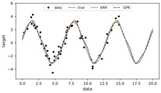
fig_18_8. Reproduces Murphy (2023), Figure 18.8. Download: PDF · SVG18.4 GPs with non-Gaussian likelihoods
p. 701, Table 18.1 Changing the likelihood gives classical models (Table 18.1); the posterior is then no longer a GP and needs approximations (see 17.2.7 in the first volume).
| Model | Likelihood | Section |
|---|---|---|
| Regression | \(\N(y_i\given f_i,\sigma_y^2)\) | 18.3.2 |
| Robust regression | \(\mathcal T_\nu(y_i\given f_i,\sigma_y^2)\) | 18.4.4 |
| Binary classification | \(\mathrm{Ber}(y_i\given\sigma(f_i))\) | 18.4.1 |
| Multiclass classification | \(\mathrm{Cat}(y_i\given\softmax(\bm f_i))\) | 18.4.2 |
| Poisson regression | \(\mathrm{Poi}(y_i\given e^{f_i})\) | 18.4.3 |
18.4.1 Binary classification
pp. 702–703, (18.100)–(18.105), Table 18.2 With labels \(y_n\in\{-1,+1\}\) and a sigmoid link, \(p(y_n\given\bm x_n)=\sigma(y_nf(\bm x_n))\); with a probit link \(\Phi(y_nf_n)\). The log joint is \[ \mathcal L(\bm f_X)=\log p(\bm y\given\bm f_X)-\tfrac12\bm f_X^\T\bm K^{-1}\bm f_X-\tfrac12\log|\bm K|-\tfrac N2\log2\pi.\tag{18.100--18.101} \] The simplest approximation is the Laplace approximation (Section 7.4.3): \(\nabla\mathcal L=\nabla\log p(\bm y\given\bm f_X)-\bm K^{-1}\bm f_X\) and \(\nabla^2\mathcal L=-\bm\Lambda-\bm K^{-1}\) with \(\bm\Lambda=-\nabla^2\log p(\bm y\given\bm f_X)\) diagonal (18.102)–(18.103); the posterior is \(q(\bm f_X)=\N(\hat{\bm f},(\bm K^{-1}+\bm\Lambda)^{-1})\) at the MAP \(\hat{\bm f}\) (18.104). Table 18.2 lists the derivatives: logistic, \(\partial_{f_i}\log\sigma(y_if_i)=t_i-\pi_i\) and \(\partial^2_{f_i}=-\pi_i(1-\pi_i)\) with \(t_i=(y_i+1)/2\), \(\pi_i=\sigma(f_i)\); probit, \(y_i\phi(f_i)/\Phi(y_if_i)\) and \(-\phi_i^2/\Phi(y_if_i)^2-y_if_i\phi(f_i)/\Phi(y_if_i)\). Variational inference with \(q=\N(\bm m,\bm S)\) is more accurate (Section 18.5.4). Prediction: from the Gaussian \(q(f_*\given\bm x_*,\mathcal D)\) and the probit approximation, \(\pi_*\approx\sigma(\kappa(v)\E[f_*])\) with \(\kappa^2(v)=(1+\pi v/8)^{-1}\) (18.105). Figure 18.9 uses an SE kernel on a 2-d problem.
Filling the gap 18.12: Laplace GP classification: derivatives, the stable Newton step, the evidence and the predictive pp. 702–703, (18.102)–(18.105), Table 18.2
Derivation
Table 18.2. Logistic, \(y\in\{-1,1\}\): \(\log\sigma(yf)=-\log(1+e^{-yf})\); the derivative is \(y(1-\sigma(yf))\), which equals \(t-\pi\) for \(y=1\) (\(t=1\), \(\pi=\sigma(f)\)) and, for \(y=-1\), \(-(1-\sigma(-f))=-\sigma(f)=t-\pi\) with \(t=0\). The second derivative is \(-\sigma(f)(1-\sigma(f))\) in both cases (since \(\sigma'=\sigma(1-\sigma)\) and \(y^2=1\)). Probit: \(\frac{\d}{\d f}\log\Phi(yf)=y\phi(yf)/\Phi(yf)=y\phi(f)/\Phi(yf)\) (\(\phi\) even), and differentiating again with \(\phi'(f)=-f\phi(f)\): \(-\phi(f)^2/\Phi(yf)^2-yf\phi(f)/\Phi(yf)\). Both second derivatives are negative (the likelihoods are log-concave), so \(\bm\Lambda\succ0\) and \(\mathcal L\) is strictly concave: the MAP is unique and Newton's method converges.
Newton step. From (18.102)–(18.103), \(\bm f^{\rm new}=\bm f-(\nabla^2\mathcal L)^{-1}\nabla\mathcal L=\bm f+(\bm K^{-1}+\bm W)^{-1}(\bm g-\bm K^{-1}\bm f)=(\bm K^{-1}+\bm W)^{-1}(\bm W\bm f+\bm g)\) with \(\bm g=\nabla\log p(\bm y\given\bm f)\) and \(\bm W=\bm\Lambda\). Using \((\bm K^{-1}+\bm W)^{-1}=\bm K-\bm K\bm W^{1/2}\bm B^{-1}\bm W^{1/2}\bm K\) with \(\bm B=\bm I+\bm W^{1/2}\bm K\bm W^{1/2}\) (Woodbury), and \(\bm b=\bm W\bm f+\bm g\): \(\bm f^{\rm new}=\bm K\bm a\), \(\bm a=\bm b-\bm W^{1/2}\bm B^{-1}\bm W^{1/2}\bm K\bm b\). This form never inverts \(\bm K\) (which can be ill conditioned) and has well-conditioned \(\bm B\) (eigenvalues \(\ge1\)); one Cholesky factor of \(\bm B\) per iteration. At the mode \(\hat{\bm f}=\bm K\bm a\) and \(\bm a=\bm K^{-1}\hat{\bm f}=\nabla\log p(\bm y\given\hat{\bm f})\) by (18.102) set to zero.
Evidence. Approximating \(\mathcal L\) by its second-order expansion at \(\hat{\bm f}\), \(\int p(\bm y\given\bm f)p(\bm f)\d\bm f\approx p(\bm y\given\hat{\bm f})\,\N(\hat{\bm f}\given\bm 0,\bm K)\,(2\pi)^{N/2}|\bm K^{-1}+\bm W|^{-1/2}\), so \[ \log q(\bm y\given\bm X)=\log p(\bm y\given\hat{\bm f})-\tfrac12\hat{\bm f}^\T\bm K^{-1}\hat{\bm f}-\tfrac12\log|\bm I+\bm W^{1/2}\bm K\bm W^{1/2}|,\] the last term being \(-\sum_n\log B_{nn}^{\rm chol}\). This equals scikit-learn's Laplace evidence for a fixed logistic GP classifier to \(10^{-3}\) in my check, and is the objective used to choose \((\ell,\sigma_f^2)\) in Figure 18.9.
Prediction. The latent mean is \(\E[f_*]=\bm k_*^\T\bm K^{-1}\hat{\bm f}=\bm k_*^\T\nabla\log p(\bm y\given\hat{\bm f})\), the variance \(k_{**}-\bm k_*^\T(\bm K+\bm W^{-1})^{-1}\bm k_*\) (conditioning \(f_*\) on a Gaussian approximation of the posterior of \(\bm f_X\)). For the class probability, use \(\sigma(a)\approx\Phi(\lambda a)\) with \(\lambda^2=\pi/8\) (matching slopes at 0); the exact integral \(\int\Phi(\lambda f)\N(f\given\mu,v)\d f=\Phi(\lambda\mu/\sqrt{1+\lambda^2v})\) and then \(\Phi(x)\approx\sigma(x/\lambda)\) give \(\sigma(\mu/\sqrt{1+\pi v/8})=\sigma(\kappa(v)\mu)\) (18.105); the derivation is also in gap 10.16 of the first volume. Over four \((\mu,v)\) pairs the approximation is within 0.02 of the exact integral.
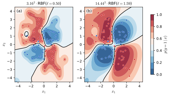
fig_18_9. Reproduces Murphy (2023), Figure 18.9. Download: PDF · SVG18.4.2 Multiclass classification
p. 703 One latent function per class, \(p(y_n\given\bm x_n)=\mathrm{Cat}(y_n\given\softmax(\bm f_n))\) with \(\bm f_n=(f_n^1,\dots,f_n^C)\) and \(f^c\sim\GP(0,K_c)\) a priori independent (the kernels may differ). The Laplace approximation is in Rasmussen and Williams, Section 3.5; variational options use a local bound on the softmax (Chai, 2012), data augmentation with auxiliary variables, or closed-form Gaussian approximations of the Bernoulli and softmax likelihoods (Miller et al., 2018; Bui, 2024): with \(\psi_k\) the logit of class \(k\) and \(\omega_k=e^{\psi_k}\sim\mathrm{Ga}(\alpha,\beta)\), moment matching replaces the likelihood by \(\N(\psi_k\given m_k,v_k)\) with \(m_k=\log(\alpha/\beta)-\tfrac12\sigma^2\), \(v_k=\sigma^2=\log(1+\beta/\alpha)\).
18.4.3 GPs for Poisson regression (Cox process)
pp. 703–705, Figures 18.10 and 18.11 With \(y_n\sim\mathrm{Poi}(e^{f(x_n)})\) and \(f\sim\GP\), the model is a Cox process: a Poisson process whose log rate is a GP. Posterior inference uses the Laplace approximation, MCMC or stochastic variational inference. In Figure 18.10 a Matérn 5/2 prior (plus a constant for the average level) is fitted by Hamiltonian Monte Carlo (Section 12.5) and by variational inference with a Gaussian \(q\). A classic application is spatial disease mapping: counts \(y_n\sim\mathrm{Poi}(e_nr_n)\) with known expected count \(e_n\) (from population and overall rate) and relative risk \(r_n\); sharing information across neighbours through \(f=\log r\sim\GP(0,K)\) with a Matérn 3/2 kernel regularises small counts (heart-attack mortality in Finland, 20 km cells).
Filling the gap 18.13: the Poisson GP: closed-form ELBO, whitened HMC and the Laplace update pp. 703–705
Derivation
Variational lower bound. For \(q(\bm f)=\N(\bm m,\bm S)\) and a prior \(\N(\bm 0,\bm K)\), \(\mathcal L(q)=\sum_n\E_q[y_nf_n-e^{f_n}-\log y_n!]-\KL(q\|p)\). The Gaussian moment-generating function gives \(\E_q[e^{f_n}]=e^{m_n+S_{nn}/2}\), so the expected log-likelihood is \(\sum_n[y_nm_n-e^{m_n+S_{nn}/2}]\) up to a constant, in closed form, and \(\KL(q\|p)=\tfrac12[\Tr(\bm K^{-1}\bm S)+\bm m^\T\bm K^{-1}\bm m-N+\log|\bm K|-\log|\bm S|]\). The bound is smooth, and was maximised with Adam over \(\bm m\) and the Cholesky factor \(\bm L_q\) of \(\bm S=\bm L_q\bm L_q^\T\) (Figure 18.10c). Only the marginals \(m_n,S_{nn}\) enter the likelihood term, which is a sum over data points, so a minibatch version (Section 18.5.4.3) applies.
Whitened MCMC. Write \(\bm f=\bm L\bm z\) with \(\bm K=\bm L\bm L^\T\) and \(\bm z\sim\N(\bm0,\bm I)\). The target \(\log p(\bm z\given\bm y)=\sum_n(y_nf_n-e^{f_n})-\tfrac12\|\bm z\|^2+\mathrm{const}\) has gradient \(\bm L^\T(\bm y-e^{\bm f})-\bm z\), and Hamiltonian Monte Carlo with a unit mass works well because the prior is already isotropic (the funnel-like dependence between \(\bm f\) and the length scale is avoided). The acceptance rate after step-size adaptation was 0.82.
Laplace update. For a Poisson likelihood with offset, \(\bm g=\bm y-\bm e\circ e^{\bm f}\) and \(\bm W=\diag(\bm e\circ e^{\bm f})\), which is positive, so Gap 18.12's Newton iteration applies unchanged; Figure 18.11 maps the relative risk \(\exp(\hat f+v/2)\) (the lognormal posterior mean) and the posterior variance of \(\log r\) on a lattice.
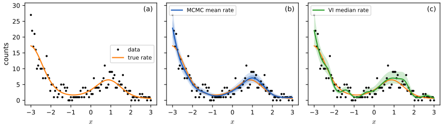
fig_18_10. Reproduces Murphy (2023), Figure 18.10. Download: PDF · SVG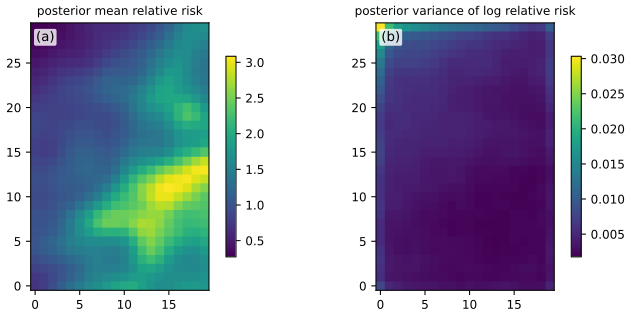
fig_18_11. Reproduces Murphy (2023), Figure 18.11. Download: PDF · SVG18.4.4 Other likelihoods
p. 704 Many other likelihoods are possible: a Student-\(t\) likelihood gives robust regression (Vanhatalo et al., 2009), and a general approach to variational inference for non-conjugate GP models is in Wilkinson, Särkkä and Solin (2021).
18.5 Scaling GP inference to large datasets
pp. 704–717, Table 18.3 Exact inference needs a Cholesky factorisation of the \(N\times N\) Gram matrix, \(O(N^3)\). The methods below scale it up; the table gives the cost of one log marginal likelihood (the bottleneck of kernel learning). \(M\) is the number of inducing points, \(B\) the minibatch size, \(D\) the input dimension, \(C\) the number of conjugate-gradient iterations and \(L\) the number of Lanczos iterations.
| Method | Cost | Section |
|---|---|---|
| Cholesky | \(O(N^3)\) | 18.3.6 |
| Conjugate gradients | \(O(CN^2)\) | 18.5.5 |
| Inducing points (SOR, DTC, FITC) | \(O(NM^2+M^3+DNM)\) | 18.5.3 |
| Variational (VFE, SGPR) | \(O(NM^2+M^3+DNM)\) | 18.5.4 |
| SVGP (minibatch) | \(O(BM^2+M^3+DNM)\) | 18.5.4.3 |
| KISS-GP | \(O(CN+CDM^D\log M)\) | 18.5.5.3 |
| SKIP | \(O(DLN+DLM\log M+L^3N\log D+CL^2N)\) | 18.5.5.3 |
See also: Introduction volume, 17.2.9 scaling GPs to large datasets.
18.5.1 Subset of data
pp. 705–706 The simplest speed-up is to throw data away: keeping \(M\) points costs \(O(M^3)\). Random subsets are the baseline (analysed by Hayakawa et al.); clustering or coreset methods pick points that cover the data with little redundancy. These are unsupervised (they ignore the \(y_i\)); a supervised alternative follows.
18.5.1.1 Informative vector machine
p. 706 The informative vector machine (IVM) greedily adds the labelled example whose inclusion lowers the entropy of the posterior of \(f\) the most, \(\Delta_j=H(p(f_j))-H(p_{\rm new}(f_j))\) (much as in active learning). Entropy is submodular, so submodular optimisation improves on the greedy choice.
Filling the gap 18.14: the IVM score is monotone in the current variance p. 706
Derivation
Before including \(y_j\), \(p(f_j)=\N(\mu_j,v_j)\). With a Gaussian observation \(y_j=f_j+\epsilon\), \(\epsilon\sim\N(0,\sigma^2)\), the new posterior is \(\propto\N(f_j\given\mu_j,v_j)\N(y_j\given f_j,\sigma^2)=\N(f_j\given\mu_j^{\rm new},v_j^{\rm new})\) with precision \((v_j^{\rm new})^{-1}=v_j^{-1}+\sigma^{-2}\). The entropy of \(\N(\mu,v)\) is \(\tfrac12\log(2\pi ev)\), so \[ \Delta_j=\tfrac12\log\frac{v_j}{v_j^{\rm new}}=\tfrac12\log\Big(v_j\big(v_j^{-1}+\sigma^{-2}\big)\Big)=\tfrac12\log\Big(1+\frac{v_j}{\sigma^2}\Big).\] It does not depend on \(y_j\) or \(\mu_j\), and is increasing in \(v_j\), so the greedy rule is "add the point with the largest current posterior variance" (the same as the maximum-variance rule of active learning with Gaussian noise). Verified numerically.
18.5.1.2 Discussion
p. 706 The drawback of subsetting is that the discarded data are ignored, which lowers accuracy and raises uncertainty; the methods below compress the data instead.
18.5.2 Nyström approximation
pp. 706–707, (18.106)–(18.116) If \(\bm K_{X,X}\approx\bm U\bm\Lambda\bm U^\T\) with the \(M\) leading eigenpairs (18.106), the matrix inversion and determinant lemmas make \(\bm K_\sigma^{-1}\) and \(|\bm K_\sigma|\) cost \(O(NM^2)\) (18.107)–(18.108); but the eigendecomposition itself costs \(O(N^3)\). Instead choose a subset \(Z\) of \(M\) points, partition the Gram matrix (18.109), eigendecompose only \(\bm K_{Z,Z}\) (eigenpairs \(\lambda_i,\bm u_i\)) and extrapolate the eigenvectors to the rest, with scalings that keep \(\|\tilde{\bm u}_i\|\approx1\): \(\tilde\lambda_i=\frac NM\lambda_i\), \(\tilde{\bm u}_i=\sqrt{M/N}\,\lambda_i^{-1}\bm K_{\tilde X,Z}\bm u_i\) (18.110)–(18.111). The result is \[ \bm K_{X,X}\approx\bm Q_{X,X}=\bm K_{X,Z}\bm K_{Z,Z}^{-1}\bm K_{Z,X},\qquad\bm Q_{A,B}\triangleq\bm K_{A,Z}\bm K_{Z,Z}^{-1}\bm K_{Z,B},\tag{18.112--18.116}\] the Nyström approximation. Replacing \(\bm K_\sigma\) by \(\hat{\bm Q}=\bm Q_{X,X}+\sigma^2\bm I\) costs \(O(NM^2)\), linear in \(N\). If only \(\bm K_\sigma\) in (18.52)–(18.53) is approximated while the other kernel terms stay exact, the predictive variance can become negative; the cure is to use \(\bm Q\) consistently everywhere.
Filling the gap 18.15: Woodbury and determinant lemmas for a low-rank-plus-diagonal matrix, and the Nyström formula pp. 706–707, (18.107)–(18.116)
Derivation
Woodbury and determinant (with the corrections to (18.107)–(18.108)). For \(\bm A,\bm C\) invertible, \((\bm A+\bm U\bm C\bm V)^{-1}=\bm A^{-1}-\bm A^{-1}\bm U(\bm C^{-1}+\bm V\bm A^{-1}\bm U)^{-1}\bm V\bm A^{-1}\) and \(|\bm A+\bm U\bm C\bm V|=|\bm C^{-1}+\bm V\bm A^{-1}\bm U|\,|\bm C|\,|\bm A|\) (first volume, Result 7.2, 7.3.4). Take \(\bm A=\sigma^2\bm I_N\), \(\bm U=\bm U\) (the \(N\times M\) orthonormal eigenvectors, \(\bm U^\T\bm U=\bm I_M\)), \(\bm C=\bm\Lambda\), \(\bm V=\bm U^\T\): \[ (\bm U\bm\Lambda\bm U^\T+\sigma^2\bm I)^{-1}=\sigma^{-2}\bm I-\sigma^{-2}\bm U\big(\sigma^2\bm\Lambda^{-1}+\bm U^\T\bm U\big)^{-1}\bm U^\T,\qquad |\bm U\bm\Lambda\bm U^\T+\sigma^2\bm I|=\sigma^{2(N-M)}\,|\bm\Lambda|\,|\sigma^2\bm\Lambda^{-1}+\bm U^\T\bm U|.\] The book's (18.107) has a plus sign in front of the second term (it must be minus: for \(M=N\), \(\bm U\) orthogonal, the right side would exceed \(\sigma^{-2}\bm I\) whereas the inverse of \(\bm K+\sigma^2\bm I\) is smaller), and (18.108) omits the factor \(\sigma^{2(N-M)}\): \(N-M\) eigenvalues equal to \(\sigma^2\) are missing from \(|\bm\Lambda|\,|\cdot|\). Both corrections are confirmed numerically (the printed forms are off by an order-one amount). Since \(\bm U^\T\bm U=\bm I\), the determinant is simply \(\sigma^{2(N-M)}\prod_i(\lambda_i+\sigma^2)\). Cost \(O(NM^2)\) (form \(\bm U^\T\bm U\) or use the \(M\times M\) matrix).
The Nyström formula. Let \(\bm K_{Z,Z}=\bm U_Z\bm\Lambda_Z\bm U_Z^\T\). Then \(\tilde{\bm u}_i\tilde{\bm u}_i^\T\tilde\lambda_i=\frac NM\lambda_i\cdot\frac MN\lambda_i^{-2}\bm K_{\tilde X,Z}\bm u_i\bm u_i^\T\bm K_{Z,\tilde X}=\lambda_i^{-1}\bm K_{\tilde X,Z}\bm u_i\bm u_i^\T\bm K_{Z,\tilde X}\); summing over \(i\) gives \(\bm K_{\tilde X,Z}\big(\sum_i\lambda_i^{-1}\bm u_i\bm u_i^\T\big)\bm K_{Z,\tilde X}=\bm K_{\tilde X,Z}\bm K_{Z,Z}^{-1}\bm K_{Z,\tilde X}\) (18.112)–(18.115): the factors \(N/M\) and \(M/N\) cancel, so the scalings are only a normalisation of the eigenvectors. The approximation is exact on the rows and columns of \(Z\) (\(\bm Q_{Z,X}=\bm K_{Z,Z}\bm K_{Z,Z}^{-1}\bm K_{Z,X}=\bm K_{Z,X}\)), has rank at most \(M\), and \(\bm K_{X,X}-\bm Q_{X,X}\) is positive semi-definite: it is the Schur complement, i.e. the covariance of \(\bm f_X\) given \(\bm f_Z\) (Gaussian conditioning). Hence \(\bm Q_{X,X}\preceq\bm K_{X,X}\): the approximation never over-states the prior variance of any linear functional. All of this agrees with a direct numerical computation.
18.5.3 Inducing point methods
pp. 707–710, (18.117)–(18.134) Introduce \(M\) inducing inputs \(\bm Z\) (pseudo-inputs) with unknown function values \(\bm f_Z\) (often written \(\bm u\)). The exact joint prior is \(p(\bm f_X,\bm f_*)=\int p(\bm f_*,\bm f_X\given\bm f_Z)p(\bm f_Z)\d\bm f_Z=\N(\bm0,\cdot)\) (18.117). Assume \(\bm f_Z\) is a sufficient statistic: \(\bm f_*\perp\bm f_X\given\bm f_Z\), so \[ p(\bm f_*,\bm f_X,\bm f_Z)=p(\bm f_*\given\bm f_X,\bm f_Z)p(\bm f_X\given\bm f_Z)p(\bm f_Z)\approx p(\bm f_*\given\bm f_Z)p(\bm f_X\given\bm f_Z)p(\bm f_Z)\tag{18.118}\] (Figure 18.12), with train and test conditionals \(p(\bm f_X\given\bm f_Z)=\N(\bm K_{X,Z}\bm K_{Z,Z}^{-1}\bm f_Z,\bm K_{X,X}-\bm Q_{X,X})\) and \(p(\bm f_*\given\bm f_Z)=\N(\bm K_{*,Z}\bm K_{Z,Z}^{-1}\bm f_Z,\bm K_{*,*}-\bm Q_{*,*})\) (18.119)–(18.120). The three methods differ in what they do to the residual covariances \(\tilde{\bm Q}_{X,X}=\bm K_{X,X}-\bm Q_{X,X}\) and \(\tilde{\bm Q}_{*,*}=\bm K_{*,*}-\bm Q_{*,*}\). All cost \(O(M^3+NM^2)\) for training, then \(O(M)\) per test mean and \(O(M^2)\) per test variance.
18.5.3.1 SOR/DIC
pp. 708–709, (18.121)–(18.124) Setting \(\tilde{\bm Q}_{X,X}=\tilde{\bm Q}_{*,*}=\bm 0\) (deterministic conditionals) is the subset of regressors (SOR) or deterministic inducing conditional (DIC) approximation: the joint prior has covariance \(\bm Q\) (18.121). With \(\hat{\bm Q}_{X,X}=\bm Q_{X,X}+\sigma^2\bm I\) and \(\bm\Sigma=(\sigma^{-2}\bm K_{Z,X}\bm K_{X,Z}+\bm K_{Z,Z})^{-1}\), \[ q_{\rm SOR}(\bm f_*\given\bm y)=\N\big(\bm Q_{*,X}\hat{\bm Q}_{X,X}^{-1}\bm y,\ \bm Q_{*,*}-\bm Q_{*,X}\hat{\bm Q}_{X,X}^{-1}\bm Q_{X,*}\big)=\N\big(\sigma^{-2}\bm K_{*,Z}\bm\Sigma\bm K_{Z,X}\bm y,\ \bm K_{*,Z}\bm\Sigma\bm K_{Z,*}\big),\tag{18.122--18.123}\] that is, exact GP inference with the degenerate kernel \(K_{\rm SOR}(\bm x_i,\bm x_j)=K(\bm x_i,\bm Z)\bm K_{Z,Z}^{-1}K(\bm Z,\bm x_j)\) (18.124), of rank \(M\); it goes to zero when \(\bm x_i\) or \(\bm x_j\) is far from \(\bm Z\), so the predictive variance is underestimated.
18.5.3.2 DTC
p. 709, (18.125)–(18.127) The deterministic training conditional keeps \(\tilde{\bm Q}_{X,X}=\bm 0\) but treats \(\tilde{\bm Q}_{*,*}=\bm K_{*,*}-\bm Q_{*,*}\) exactly. The predictive mean is the same as in SOR and the variance is larger, \(\bm K_{*,*}-\bm Q_{*,*}+\bm K_{*,Z}\bm\Sigma\bm K_{Z,*}\) (18.127), because \(\bm K_{*,*}-\bm Q_{*,*}\succeq0\), which cures the overconfidence of SOR far from the inducing points.
18.5.3.3 FITC
pp. 709–710, (18.128)–(18.131) The fully independent training conditional assumes the training function values are conditionally independent given \(\bm f_Z\): \(q(\bm f_X\given\bm f_Z)=\N(\bm K_{X,Z}\bm K_{Z,Z}^{-1}\bm f_Z,\ \diag(\bm K_{X,X}-\bm Q_{X,X}))\) (18.128). The joint prior has training block \(\bm Q_{X,X}-\diag(\bm Q_{X,X}-\bm K_{X,X})\) (18.129) and, with \(\bm\Lambda=\diag(\bm K_{X,X}-\bm Q_{X,X}+\sigma^2\bm I)\), \(\bm\Sigma=(\bm K_{Z,Z}+\bm K_{Z,X}\bm\Lambda^{-1}\bm K_{X,Z})^{-1}\), \[ q_{\rm fitc}(f_*\given\bm y)=\N\big(\bm k_{*,Z}\bm\Sigma\bm K_{Z,X}\bm\Lambda^{-1}\bm y,\ k_{**}-q_{**}+\bm k_{*,Z}\bm\Sigma\bm k_{Z,*}\big).\tag{18.130}\] For a batch of test points one assumes conditional independence (FIC). FITC is equivalent to exact GP inference with the non-degenerate kernel \(K_{\rm fic}(\bm x_i,\bm x_j)=K(\bm x_i,\bm x_i)\) if \(i=j\), \(K_{\rm SOR}(\bm x_i,\bm x_j)\) otherwise (18.131). Because it keeps the diagonal of the residual it never claims more certainty than the prior at a data point.
Filling the gap 18.16: one formula for SOR, DTC and FITC pp. 708–710, (18.121)–(18.131)
Derivation
Write \(\bm U=\bm K_{X,Z}\), \(\bm K_{Z,Z}=\bm K_{ZZ}\) and consider the approximate model in which the training function values have prior covariance \(\bm Q_{X,X}+\bm D\) and the cross-covariance with the test values is \(\bm Q_{X,*}\), where \(\bm D=\bm0\) for SOR and DTC and \(\bm D=\diag(\bm K_{X,X}-\bm Q_{X,X})\) for FITC. Let \(\bm\Lambda=\bm D+\sigma^2\bm I\), \(\bm\Sigma=(\bm K_{ZZ}+\bm U^\T\bm\Lambda^{-1}\bm U)^{-1}\). Gaussian conditioning gives mean \(\bm Q_{*,X}(\bm Q_{X,X}+\bm\Lambda)^{-1}\bm y\) and covariance \(\bm Q_{*,*}'-\bm Q_{*,X}(\bm Q_{X,X}+\bm\Lambda)^{-1}\bm Q_{X,*}\), where the prior test covariance \(\bm Q_{*,*}'\) is \(\bm Q_{*,*}\) (SOR) or \(\bm K_{*,*}\) (DTC, FITC).
Key identity. By Woodbury, \((\bm Q+\bm\Lambda)^{-1}=\bm\Lambda^{-1}-\bm\Lambda^{-1}\bm U\bm\Sigma\bm U^\T\bm\Lambda^{-1}\) (with \(\bm Q=\bm U\bm K_{ZZ}^{-1}\bm U^\T\), since \(\bm K_{ZZ}+\bm U^\T\bm\Lambda^{-1}\bm U=\bm\Sigma^{-1}\)). Using \(\bm U^\T\bm\Lambda^{-1}\bm U=\bm\Sigma^{-1}-\bm K_{ZZ}\), \[ \bm K_{ZZ}^{-1}\bm U^\T(\bm Q+\bm\Lambda)^{-1}=\bm K_{ZZ}^{-1}\big[\bm I-\bm U^\T\bm\Lambda^{-1}\bm U\bm\Sigma\big]\bm U^\T\bm\Lambda^{-1}=\bm K_{ZZ}^{-1}\big[\bm I-(\bm\Sigma^{-1}-\bm K_{ZZ})\bm\Sigma\big]\bm U^\T\bm\Lambda^{-1}=\bm\Sigma\,\bm U^\T\bm\Lambda^{-1}.\] Multiplying on the left by \(\bm K_{*,Z}\): mean \(\bm Q_{*,X}(\bm Q+\bm\Lambda)^{-1}\bm y=\bm K_{*,Z}\bm\Sigma\bm K_{Z,X}\bm\Lambda^{-1}\bm y\). With \(\bm\Lambda=\sigma^2\bm I\) this is (18.123) (SOR, DTC) and with \(\bm\Lambda=\diag(\cdot)+\sigma^2\bm I\) it is (18.130) (FITC). For the variance, \(\bm Q_{*,X}(\bm Q+\bm\Lambda)^{-1}\bm Q_{X,*}=\bm K_{*,Z}\bm\Sigma\bm U^\T\bm\Lambda^{-1}\bm U\bm K_{ZZ}^{-1}\bm K_{Z,*}=\bm K_{*,Z}\bm\Sigma(\bm\Sigma^{-1}-\bm K_{ZZ})\bm K_{ZZ}^{-1}\bm K_{Z,*}=\bm Q_{*,*}-\bm K_{*,Z}\bm\Sigma\bm K_{Z,*}\), hence \[ \text{variance}=\bm Q_{*,*}'-\bm Q_{*,*}+\bm K_{*,Z}\bm\Sigma\bm K_{Z,*}=\begin{cases}\bm K_{*,Z}\bm\Sigma\bm K_{Z,*}&\text{SOR (18.123)}\\\bm K_{*,*}-\bm Q_{*,*}+\bm K_{*,Z}\bm\Sigma\bm K_{Z,*}&\text{DTC, FITC (18.127), (18.130)}\end{cases}\] So SOR and DTC have the same mean and DTC's variance exceeds SOR's by \(\bm K_{*,*}-\bm Q_{*,*}\succeq0\) (the Schur complement, Gap 18.15). Far from \(\bm Z\), \(\bm K_{*,Z}\to0\): SOR variance \(\to0\), DTC variance \(\to k_{**}\) (the prior). FIC kernel. The training covariance \(\bm Q_{X,X}+\diag(\bm K_{X,X}-\bm Q_{X,X})\) has diagonal \(K(\bm x_i,\bm x_i)\) and off-diagonal \(K_{\rm SOR}(\bm x_i,\bm x_j)\): (18.131); it has full rank, so FITC is a genuine (non-degenerate) GP, in contrast to the rank-\(M\) SOR. The dense formulas, the \(O(NM^2)\) implementation, and the forms (18.123) and (18.130) agree to \(10^{-7}\) in a numerical experiment, and for a single inducing point at the location of all the data the SOR variance is \(k(x_*,0)^2/(1+n/\sigma^2)\) (practice problem 18.3).
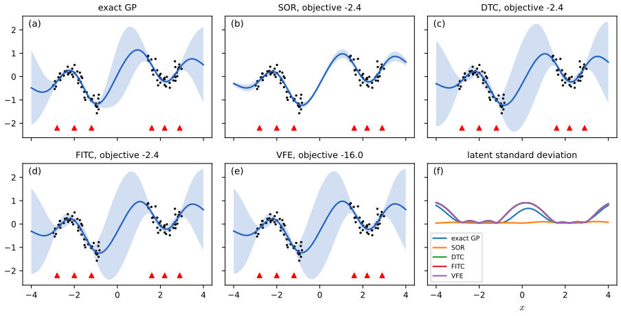
fig_S18_2. Download: PDF · SVG18.5.3.4 Learning the inducing points
pp. 710–711, (18.132)–(18.134), Figure 18.13 The inducing inputs can be learned like hyper-parameters, by maximising the log marginal likelihood of the approximate model, \[ \log q(\bm y\given\bm X,\bm Z)=\log\!\int p(\bm y\given\bm f_X)q(\bm f_X\given\bm X,\bm Z)\d\bm f_X=-\tfrac12\log|\bm Q_{X,X}+\bm\Lambda|-\tfrac12\bm y^\T(\bm Q_{X,X}+\bm\Lambda)^{-1}\bm y-\tfrac N2\log2\pi,\tag{18.132--18.134}\] with \(\bm\Lambda_{\rm SOR}=\bm\Lambda_{\rm DTC}=\sigma^2\bm I\) and \(\bm\Lambda_{\rm fitc}=\diag(\bm K_{X,X}-\bm Q_{X,X})+\sigma^2\bm I\). If the inputs are in \(\R^d\), \(\bm Z\in\R^{Md}\) is optimised by gradients. For structured inputs (strings, graphs) one selects \(\bm Z\) from the training set or uses discrete optimisation such as simulated annealing (Figure 18.13, DNA sequences). Treating \(\bm Z\) as a model parameter in this way risks overfitting; the next section treats it as a variational parameter instead.
18.5.4 Sparse variational methods
pp. 710–714, (18.135)–(18.159) The sparse variational GP (SVGP, also the variational free energy or VFE approach; Titsias, 2009) keeps the model exact and approximates the posterior. Partition a (finite or discretised) input set into training inputs \(X\), inducing inputs \(Z\) and the rest \(X_*\), and let \(\bm f=[\bm f_X,\bm f_Z,\bm f_*]\). The approximating family is \[ q(\bm f)=p(\bm f_*,\bm f_X\given\bm f_Z)\,q(\bm f_Z),\] exact conditionals from the GP prior and a free \(q(\bm f_Z)\). The inducing values act as a bottleneck that absorbs all of \(\bm y\); \(\bm Z\) and \(\bm f_Z\) are variational parameters, so they cannot overfit, and as \(M\) grows the posterior approximation improves (it reaches the exact one at \(\bm Z=\bm X\)). Minimising \(\KL(q(\bm f)\|p(\bm f\given\bm y))\) is the same as maximising \[ \log p(\bm y)=\KL(q\|p(\cdot\given\bm y))+\E_{q(\bm f_X)}[\log p(\bm y\given\bm f_X)]-\KL(q(\bm f_Z)\|p(\bm f_Z))\ \ge\ \mathcal L(q)=\E_{q(\bm f_X)}[\log p(\bm y\given\bm f_X)]-\KL(q(\bm f_Z)\|p(\bm f_Z)).\tag{18.135--18.142}\] With a Gaussian \(q(\bm f_Z)=\N(\bm m,\bm S)\) the KL term is closed form (KL between Gaussians, (5.77)) and the induced marginal at a training input is \(q(\bm f_X)=\N(\tilde{\bm\mu},\tilde{\bm\Sigma})\), \[ \tilde\mu_i=m(\bm x_i)+\bm\alpha(\bm x_i)^\T(\bm m-m(\bm Z)),\quad\tilde\Sigma_{ij}=K(\bm x_i,\bm x_j)-\bm\alpha(\bm x_i)^\T(\bm K_{Z,Z}-\bm S)\bm\alpha(\bm x_j),\quad\bm\alpha(\bm x_i)=\bm K_{Z,Z}^{-1}\bm K_{Z,\bm x_i},\tag{18.143--18.146}\] and the likelihood term is a sum \(\sum_n\E_{q(f_n)}[\log p(y_n\given f_n)]\) of one-dimensional expectations (18.147).
Filling the gap 18.17: the variational bound, the optimal \(q(\bm f_Z)\), the collapsed bound and its monotonicity in \(M\) pp. 710–714, (18.135)–(18.158)
Derivation
The KL identity (18.135)–(18.140). Bayes' rule on all function values gives \(p(\bm f_*,\bm f_X,\bm f_Z\given\bm y)=p(\bm y\given\bm f_X)\,p(\bm f_*,\bm f_X\given\bm f_Z)\,p(\bm f_Z)/p(\bm y)\) (the likelihood depends on \(\bm f_X\) only). The variational family has the same factor \(p(\bm f_*,\bm f_X\given\bm f_Z)\), so in the ratio \[ \frac{q(\bm f)}{p(\bm f\given\bm y)}=\frac{p(\bm f_*,\bm f_X\given\bm f_Z)q(\bm f_Z)\,p(\bm y)}{p(\bm y\given\bm f_X)p(\bm f_*,\bm f_X\given\bm f_Z)p(\bm f_Z)}=\frac{q(\bm f_Z)\,p(\bm y)}{p(\bm f_Z)\,p(\bm y\given\bm f_X)}\] the conditional cancels (the crossed-out terms in (18.137)). Taking \(\E_q\log\) gives \(\KL(q\|p(\cdot\given\bm y))=\KL(q(\bm f_Z)\|p(\bm f_Z))-\E_{q(\bm f_X)}[\log p(\bm y\given\bm f_X)]+\log p(\bm y)\) (18.140), so \(\mathcal L(q)\le\log p(\bm y)\) (18.141)–(18.142) since \(\KL\ge0\). (The footnote's claim that \(\KL(q(\bm f)\|p(\bm f\given\bm y))=\KL(q(\bm f_X,\bm f_Z)\|p(\bm f_X,\bm f_Z\given\bm y))\) follows because the extra factor \(p(\bm f_*\given\bm f_X,\bm f_Z)\) is common to \(q\) and \(p\).)
Optimal \(q(\bm f_Z)\) and the collapsed bound. For fixed \(\bm Z\), \(\mathcal L(q)=-\KL(q(\bm f_Z)\|p(\bm f_Z))+\E_{q(\bm f_Z)}[g(\bm f_Z)]\) with \(g(\bm f_Z)=\E_{p(\bm f_X\given\bm f_Z)}[\log p(\bm y\given\bm f_X)]\). By the Gibbs variational principle (gap 14.2) the maximiser is \(q^*(\bm f_Z)\propto p(\bm f_Z)e^{g(\bm f_Z)}\) and the maximum is \(\log\int p(\bm f_Z)e^{g(\bm f_Z)}\d\bm f_Z\). For the Gaussian likelihood \(\N(\bm y\given\bm f_X,\sigma^2\bm I)\) and \(p(\bm f_X\given\bm f_Z)=\N(\bm A\bm f_Z,\bm K_{X,X}-\bm Q_{X,X})\), \(\bm A=\bm K_{X,Z}\bm K_{Z,Z}^{-1}\): \[ g(\bm f_Z)=\log\N(\bm y\given\bm A\bm f_Z,\sigma^2\bm I)-\frac1{2\sigma^2}\Tr(\bm K_{X,X}-\bm Q_{X,X}),\] since \(\E[(\bm y-\bm f_X)^\T(\bm y-\bm f_X)]=\|\bm y-\bm A\bm f_Z\|^2+\Tr(\mathrm{cov})\). Then \(\int\N(\bm f_Z\given\bm0,\bm K_{ZZ})\N(\bm y\given\bm A\bm f_Z,\sigma^2\bm I)\d\bm f_Z=\N(\bm y\given\bm 0,\bm A\bm K_{ZZ}\bm A^\T+\sigma^2\bm I)=\N(\bm y\given\bm0,\bm Q_{X,X}+\sigma^2\bm I)\), so \[ \log p(\bm y)\ \ge\ \log\N(\bm y\given\bm0,\bm Q_{X,X}+\sigma^2\bm I)-\frac1{2\sigma^2}\Tr(\bm K_{X,X}-\bm Q_{X,X}),\tag{18.158}\] the collapsed bound (\(\bm f_Z\) integrated out). The optimal \(q^*\) is the Gaussian \(\propto p(\bm f_Z)\N(\bm y\given\bm A\bm f_Z,\sigma^2\bm I)\) with precision \(\bm\Lambda=\bm K_{ZZ}^{-1}+\beta\bm K_{ZZ}^{-1}\bm K_{Z,X}\bm K_{X,Z}\bm K_{ZZ}^{-1}\) (\(\beta=\sigma^{-2}\)) and mean \(\bm m=\beta\bm\Lambda^{-1}\bm K_{ZZ}^{-1}\bm K_{Z,X}\bm y\), i.e. \(\bm S=\bm\Lambda^{-1}\) (18.155)–(18.157). I verified numerically that the ELBO (18.149)–(18.150) evaluated at this \((\bm m,\bm S)\) equals (18.158) to \(10^{-8}\), and that any perturbation of \(\bm m\) or scaling of \(\bm S\) lowers it.
Relation to DTC and the role of the trace. The first term of (18.158) is the DTC marginal likelihood (18.134) with \(\bm\Lambda=\sigma^2\bm I\); the extra \(-\Tr(\bm K_{X,X}-\bm Q_{X,X})/(2\sigma^2)\le0\) penalises inducing sets that fail to capture the prior variance at the data. It is this term that prevents the marginal-likelihood overfitting that DTC can show when \(\bm Z\) is optimised, and the optimal \(q^*\) gives the same predictive distribution as DTC. If \(\bm Z=\bm X\) then \(\bm Q_{X,X}=\bm K_{X,X}\), the trace vanishes and the bound equals \(\log p(\bm y)=\log\N(\bm y\given\bm0,\bm K_{X,X}+\sigma^2\bm I)\): it is tight.
More inducing points never hurt. Let \(\bm Z\subset\bm Z'\) and let \(q(\bm f_Z)\) be any variational distribution for the smaller set. Define \(q'(\bm f_{Z'})=p(\bm f_{Z'\setminus Z}\given\bm f_Z)\,q(\bm f_Z)\), which belongs to the larger family. Apply the identity (18.140) with \(\bm Z'\) as the inducing set: \(\KL(q'(\bm f_{Z'})\|p(\bm f_{Z'}))=\KL(q(\bm f_Z)\|p(\bm f_Z))\) because the two densities share the factor \(p(\bm f_{Z'\setminus Z}\given\bm f_Z)\); and the marginal of \(\bm f_X\) under \(q'\) is \(\int p(\bm f_X\given\bm f_{Z'})p(\bm f_{Z'\setminus Z}\given\bm f_Z)q(\bm f_Z)\d\bm f_{Z'}=\int p(\bm f_X\given\bm f_Z)q(\bm f_Z)\d\bm f_Z\), the same as under \(q\) (marginalising the GP prior over \(\bm f_{Z'\setminus Z}\)). So \(\mathcal L'(q')=\mathcal L(q)\): the larger family contains a member with exactly the same bound, hence the optimised bound is non-decreasing along nested inducing sets. Numerically, for \(M=4,8,16,40\) inducing points spread evenly over the 40 data inputs the bound goes \(-88.4,-5.94,-5.26,-5.26\) against \(\log p(\bm y)=-5.26\). (The classical DTC/FITC objective does not have this monotonicity, which is the book's remark that more inducing points do not always help there.)
18.5.4.1 Gaussian likelihood
pp. 712–713, (18.148)–(18.158) With a Gaussian observation model with precision \(\beta=\sigma^{-2}\) and \(m(\bm x)=0\), the expected log-likelihood is closed form, \[ \E_{q(f_n)}[\log\N(y_n\given f_n,\beta^{-1})]=\log\N(y_n\given\bm k_n^\T\bm K_{ZZ}^{-1}\bm m,\beta^{-1})-\tfrac12\beta\tilde k_{nn}-\tfrac12\Tr(\bm S\bm\Lambda_n),\tag{18.148}\] with \(\tilde k_{nn}=k_{nn}-\bm k_n^\T\bm K_{ZZ}^{-1}\bm k_n\), \(\bm k_n\) the \(n\)-th column of \(\bm K_{Z,X}\) and \(\bm\Lambda_n=\beta\bm K_{ZZ}^{-1}\bm k_n\bm k_n^\T\bm K_{ZZ}^{-1}\), so the ELBO is \[ \mathcal L(q)=\log\N(\bm y\given\bm K_{X,Z}\bm K_{ZZ}^{-1}\bm m,\beta^{-1}\bm I)-\tfrac\beta2\Tr(\bm K_{X,Z}\bm K_{ZZ}^{-1}\bm S\bm K_{ZZ}^{-1}\bm K_{Z,X})-\tfrac\beta2\Tr(\bm K_{X,X}-\bm Q_{X,X})-\KL(q(\bm f_Z)\|p(\bm f_Z)).\tag{18.149--18.150}\] The gradients \(\nabla_{\bm m}\mathcal L=\beta\bm K_{ZZ}^{-1}\bm K_{Z,X}\bm y-\bm\Lambda\bm m\) and \(\nabla_{\bm S}\mathcal L=\tfrac12\bm S^{-1}-\tfrac12\bm\Lambda\) (18.153)–(18.154) vanish at (18.155)–(18.157), the sparse GP regression (SGPR) solution of Titsias, with collapsed bound (18.158) (Gap 18.17 above). If \(\bm Z=\bm X\) the bound is tight. The only difference from the DTC likelihood is the trace term.
18.5.4.2 Non-Gaussian likelihood
p. 713 For non-Gaussian likelihoods, with \(h(f_n)=\log p(y_n\given f_n)\), the gradients of the expectation are \(\E[h']\) and \(\tfrac12\E[h'']\) (18.151)–(18.152), estimated by Monte Carlo or numerical quadrature (Section 8.5.1.4). For a binary classifier, Table 18.2 gives \(h'\) and \(h''\).
Filling the gap 18.18: the Price/Bonnet identities and the closed-form expected log-likelihood pp. 712–713, (18.148), (18.151)–(18.154)
Derivation
(18.151)–(18.152). Let \(\varphi(x;\mu,v)=\N(x\given\mu,v)\) and \(h\) a smooth function with enough decay. Since \(\varphi\) depends on \(x-\mu\), \(\partial_\mu\varphi=-\partial_x\varphi\); integrating by parts, \(\partial_\mu\E[h]=-\int h\,\partial_x\varphi=\int h'\varphi=\E[h']\). The Gaussian density solves the heat equation \(\partial_v\varphi=\tfrac12\partial_x^2\varphi\) (check: \(\partial_v\varphi=\varphi[-\tfrac1{2v}+\tfrac{(x-\mu)^2}{2v^2}]\) and \(\partial_x^2\varphi=\varphi[\tfrac{(x-\mu)^2}{v^2}-\tfrac1v]\)); integrating by parts twice, \(\partial_v\E[h]=\tfrac12\int h\,\partial_x^2\varphi=\tfrac12\E[h'']\). Both identities agree with numerical differentiation of the Gaussian expectation of a test function.
(18.148). For \(f_n\sim\N(\mu_n,v_n)\), \(\E[\log\N(y_n\given f_n,\beta^{-1})]=-\tfrac12\log(2\pi\beta^{-1})-\tfrac\beta2[(y_n-\mu_n)^2+v_n]=\log\N(y_n\given\mu_n,\beta^{-1})-\tfrac\beta2v_n\). Here \(\mu_n=\bm k_n^\T\bm K_{ZZ}^{-1}\bm m\) and, from (18.145), \(v_n=\tilde\Sigma_{nn}=\tilde k_{nn}+\bm k_n^\T\bm K_{ZZ}^{-1}\bm S\bm K_{ZZ}^{-1}\bm k_n\); the second part equals \(\tfrac12\Tr(\bm S\bm\Lambda_n)\) with \(\bm\Lambda_n\) as in the text, giving (18.148). (The check by quadrature agrees to \(10^{-8}\).) (18.153)–(18.154). \(\nabla_{\bm m}\log\N(\bm y\given\bm A\bm m,\beta^{-1}\bm I)=\beta\bm A^\T(\bm y-\bm A\bm m)\) with \(\bm A=\bm K_{X,Z}\bm K_{ZZ}^{-1}\), and \(\nabla_{\bm m}\tfrac12\bm m^\T\bm K_{ZZ}^{-1}\bm m=\bm K_{ZZ}^{-1}\bm m\); so \(\nabla_{\bm m}\mathcal L=\beta\bm A^\T\bm y-(\beta\bm A^\T\bm A+\bm K_{ZZ}^{-1})\bm m\), and \(\beta\bm A^\T\bm A+\bm K_{ZZ}^{-1}=\bm\Lambda\) of (18.156). For \(\bm S\): \(-\tfrac\beta2\Tr(\bm A\bm S\bm A^\T)\) has gradient \(-\tfrac\beta2\bm A^\T\bm A\), and the KL has \(\nabla_{\bm S}[\tfrac12\Tr(\bm K_{ZZ}^{-1}\bm S)-\tfrac12\log|\bm S|]=\tfrac12\bm K_{ZZ}^{-1}-\tfrac12\bm S^{-1}\); the sum is \(\tfrac12\bm S^{-1}-\tfrac12\bm\Lambda\).
18.5.4.3 Minibatch SVI
p. 714, (18.159) Solving for \((\bm m,\bm S)\) in closed form is a batch computation, \(O(M^3+NM^2)\), still heavy for large \(N\) unless \(M\) is small. Because the likelihood term is a sum over data, a minibatch gives an unbiased estimate (Hensman et al., 2013): \(\mathcal L(q)\approx\frac NB\sum_{b=1}^B\frac1{|\mathcal B_b|}\sum_{n\in\mathcal B_b}\E_{q(f_n)}[\log p(y_n\given f_n)]-\KL(q(\bm f_Z)\|p(\bm f_Z))\) (18.159) (the book writes the sum over \(B\) batches; in Table 18.3 \(B\) is the minibatch size). With a Gaussian likelihood the model is in the exponential family, so the natural gradient (Section 6.4) in the natural parameters of \(q(\bm f_Z)\) converges much faster than the ordinary gradient.
18.5.5 Exploiting parallelization and structure via kernel matrix multiplies
pp. 714–716 The Cholesky factorisation is largely sequential and costs \(O(N^3)\). Krylov subspace methods need only matrix–vector multiplies (MVMs), which parallelise trivially on GPUs and are fast when \(\bm K\) has structure.
18.5.5.1 Using conjugate gradient and Lanczos methods
pp. 714–715, Figure 18.14 Conjugate gradients (CG) solve \(\bm K_\sigma\bm\alpha=\bm y\) with \(C\) MVMs, in \(O(C\tau(\bm K_\sigma))\) time where \(\tau\) is the cost of one MVM (\(n^2\) for a dense matrix; less if \(\bm K\) is sparse or structured). With \(C=n\) it is exact in \(O(n^3)\), but usually far fewer iterations suffice, depending on the condition number. The log determinant is computed from MVMs by stochastic Lanczos quadrature, \(O(L\tau)\) for \(L\) iterations. These are the core of black-box matrix–matrix multiplication (BBMM) inference, which makes exact GP inference possible for \(N\sim10^4\) points in seconds, \(10^5\) in minutes and \(10^6\) in hours on 8 GPUs (Wang et al., 2019). Figure 18.14 (from that paper) shows that exact GP inference on a subset can beat approximate inference on all the data, and that exact GPs keep improving as \(N\) grows: an exact method with a non-degenerate kernel keeps its non-parametric capacity, while the standard approximations replace the kernel by one corresponding to a parametric model.
Filling the gap 18.19: why conjugate gradients converge fast on a kernel matrix, and how stochastic Lanczos quadrature gets \(\log|\bm K_\sigma|\) pp. 714–715
Derivation
CG error bound. Let \(\bm A=\bm K_\sigma\succ0\), \(\bm\alpha^*=\bm A^{-1}\bm y\), \(\bm\alpha_0=\bm0\), \(\bm e_j=\bm\alpha_j-\bm\alpha^*\). CG's iterate minimises the \(\bm A\)-norm of the error over the Krylov space: \(\bm e_j=p(\bm A)\bm e_0\) with \(p\) a polynomial of degree \(\le j\), \(p(0)=1\), chosen optimally. In the eigenbasis of \(\bm A\), \(\|\bm e_j\|_{\bm A}\le\min_p\max_{i}|p(\lambda_i)|\,\|\bm e_0\|_{\bm A}\). Bounding the maximum over the spectrum by the maximum over \([\lambda_{\min},\lambda_{\max}]\) and using the Chebyshev polynomial that is smallest on that interval, \[ \|\bm e_j\|_{\bm A}\le2\Big(\frac{\sqrt\kappa-1}{\sqrt\kappa+1}\Big)^j\|\bm e_0\|_{\bm A},\qquad\kappa=\frac{\lambda_{\max}}{\lambda_{\min}}.\] For \(\bm K_\sigma=\bm K+\sigma^2\bm I\), \(\lambda_{\min}\ge\sigma^2\) and \(\lambda_{\max}\le\sigma^2+N\max k\), so \(\kappa\le1+N\max k/\sigma^2\) (the noise regularises the system). The bound is pessimistic for kernel matrices, whose eigenvalues decay fast (Gap 18.5): \(p\) of degree \(j\) can place roots at the \(j\) largest eigenvalues, so the error is governed by the remaining small cluster. In the numerical experiment (\(N=200\), \(\kappa=102\)) the observed error is below the bound at every iteration and CG has solved the system to \(3\times10^{-14}\) after 40 iterations.
Log determinant. \(\log|\bm A|=\Tr\log\bm A\). Hutchinson's estimator: for random \(\bm z\) with \(\E[\bm z\bm z^\T]=\bm I\) (e.g. Rademacher entries), \(\E[\bm z^\T\log(\bm A)\bm z]=\Tr\log\bm A\); Rademacher vectors have the smallest variance, \(2(\|\log\bm A\|_F^2-\sum_i[\log\bm A]_{ii}^2)\). Each quadratic form is estimated by Lanczos: running \(m\) steps from \(\bm q_1=\bm z/\|\bm z\|\) gives \(\bm A\bm Q_m=\bm Q_m\bm T_m+\ldots\) with tridiagonal \(\bm T_m\), and \(\bm z^\T f(\bm A)\bm z\approx\|\bm z\|^2\bm e_1^\T f(\bm T_m)\bm e_1\). This is a Gauss quadrature for the spectral measure of \(\bm A\) at \(\bm q_1\): it is exact for polynomials \(f\) of degree \(\le2m-2\), because \(\bm A^a\bm q_1=\bm Q_m\bm T_m^a\bm e_1\) for \(a\le m-1\) (the Krylov space is invariant up to that power), so \(\bm q_1^\T\bm A^{a+b}\bm q_1=(\bm A^a\bm q_1)^\T(\bm A^b\bm q_1)=(\bm T^a\bm e_1)^\T(\bm T^b\bm e_1)\) for \(a,b\le m-1\). Since \(\log\) is smooth on the spectrum \([\sigma^2,\lambda_{\max}]\), Lanczos converges fast: in an example (a \(200\times200\) SE-kernel matrix with noise variance 0.5) \(m=10\) steps already give each quadratic form to two decimals. The remaining error is the Hutchinson sampling error, which falls like the inverse square root of the number of probes: with 200 Rademacher probes the estimate of \(\log|\bm K_\sigma|\) is within 2% of the exact value (for example \(-103.6\) against \(-105.3\)).
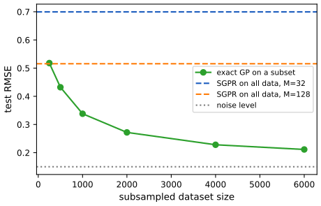
fig_18_14. Reproduces Murphy (2023), Figure 18.14. Download: PDF · SVG18.5.5.2 Kernels with compact support
p. 715 If \(K(\bm x,\bm x')=0\) whenever \(\|\bm x-\bm x'\|>\epsilon\) the matrix \(\bm K_\sigma\) is sparse and an MVM costs \(O(N)\) (Melkumyan and Ramos, 2009).
18.5.5.3 KISS
pp. 715–716, (18.160) Structured kernel interpolation (SKI) forces structure: choose inducing points \(\bm Z\) and interpolate, \(\bm K_{X,X}\approx\bm W_X\bm K_{Z,Z}\bm W_X^\T\) with a sparse interpolation matrix \(\bm W_X\) (cubic interpolation: 4 non-zeros per row), so \(\bm W\bm K_{ZZ}\bm W^\T\bm v\) costs \(O(N+M^2)\). SKI generalises the inducing-point methods: \(\bm W=\bm K_{X,Z}\bm K_{ZZ}^{-1}\) is SOR. In 1-d with a regular grid \(\bm K_{ZZ}\) is Toeplitz and the MVM costs \(O(N+M\log M)\); in \(D\) dimensions a grid gives a Kronecker product of Toeplitz matrices (KISS-GP), but the number of grid points is exponential in \(D\). SKIP (SKI for products) exploits \(K=\prod_dK_d\) with 1-d SKI and Lanczos, at cost \(O(DL(N+M\log M)+L^3N\log D+CL^2N)\). Tensor-train methods (TT-GP) represent the variational mean and covariance in Kronecker/tensor-train form and scale to billions of inducing points.
Filling the gap 18.20: FFT multiplication by a Toeplitz matrix, the order of SKI, and SOR as SKI pp. 715–716, (18.160)
Derivation
Toeplitz MVM. A symmetric Toeplitz matrix \(\bm T=(c_{|i-j|})_{i,j<M}\) embeds in the circulant matrix \(\bm C\) of size \(2M-2\) whose first column is \((c_0,\dots,c_{M-1},c_{M-2},\dots,c_1)\). A circulant matrix is diagonalised by the discrete Fourier transform, \(\bm C\bm w=\mathcal F^{-1}[\mathcal F(\bm c)\circ\mathcal F(\bm w)]\), so \(\bm T\bm v\) is the first \(M\) entries of \(\bm C[\bm v;\bm0]\), computed in \(O(M\log M)\) with two forward FFTs and one inverse FFT (the FFT of the kernel column is computed once). Verified against the dense product.
Accuracy. With linear interpolation between grid points a distance \(h\) apart, \(W\)-weighted sum of \(K\) at the neighbouring grid points has error \(\le\frac{h^2}8\sup|\partial^2K|\) (the classical linear-interpolation bound applied to the smooth function \(K(\cdot,x')\)); cubic interpolation gives \(O(h^4)\). Halving \(h\) divides the error by about 4 in my check (ratio 4.0 for \(M=64\) vs \(127\)), and the SKI Gram matrix with 64 points is within \(10^{-2}\) of the exact one on 50 random inputs. SOR as SKI. Taking \(\bm W=\bm K_{X,Z}\bm K_{ZZ}^{-1}\) (the "global interpolation" onto the inducing points) gives \(\bm W\bm K_{ZZ}\bm W^\T=\bm K_{X,Z}\bm K_{ZZ}^{-1}\bm K_{Z,X}=\bm Q_{X,X}\), the SOR kernel (18.124); the interpolation weights are then dense, which is why local (sparse) interpolation is what makes SKI fast.
18.5.5.4 Tensor train methods
p. 716 In the variational method of Section 18.5.4 one stores the mean \(\bm m\) and the covariance \(\bm S\) of \(q(\bm f_Z)\). \(\bm S\) can be given Kronecker structure as in KISS, and \(\bm m\) a tensor-train decomposition (Oseledets), combined with SKI: the TT-GP method scales to billions of inducing points (Izmailov et al.).
18.5.6 Converting a GP to an SSM
pp. 716–717, and Supplement 18.2 For a function of a scalar input such as time, many stationary kernels correspond to a linear time-invariant stochastic differential equation (SDE), which can be discretised into a linear-Gaussian state space model (SSM; Härkönen and Särkkä, 2010). The exponential kernel (Matérn 1/2) corresponds to the Ornstein–Uhlenbeck SDE \(\d x/\d t=-\lambda x+w(t)\) with white noise of spectral density \(q\); the condition for an SDE representation is that the spectral density is a rational function, which holds for the Matérn family and excludes the SE kernel (approximable). Kernels such as Matérn 3/2 need several latent states, and higher-dimensional inputs even more (to keep the Markov property). Kalman smoothing (Section 8.2.3) then gives exact inference in \(O(N)\) time, or \(O(\log N)\) span on a parallel machine.
The supplement (Section 18.2 there) gives the matrices. For the Matérn kernel with \(\nu=\tfrac32\), length scale \(\ell\) and variance \(\sigma^2\), with \(\lambda=\sqrt3/\ell\), \[ \bm F=\begin{pmatrix}0&1\\-\lambda^2&-2\lambda\end{pmatrix},\quad\bm L=\begin{pmatrix}0\\1\end{pmatrix},\quad\bm H=\begin{pmatrix}1&0\end{pmatrix},\tag{S18.14}\] and for \(\nu=\tfrac52\), \(\lambda=\sqrt5/\ell\), \(p=\nu-\tfrac12\), \(\bm F=\begin{pmatrix}0&1&0\\0&0&1\\-\lambda^3&-3\lambda^2&-3\lambda\end{pmatrix}\), \(\bm L=(0,0,1)^\T\), \(\bm H=(1,0,0)\) with \(q=2\sigma^2\sqrt\pi\lambda^{2p+1}\Gamma(p+1)/\Gamma(p+\tfrac12)\) (S18.16)–(S18.17). With \(\Delta_k=t_k-t_{k-1}\), \(\bm z_k=\bm A_{k-1}\bm z_{k-1}+\N(\bm0,\bm Q_{k-1})\), \(y_k=\bm H\bm z_k+\N(0,\sigma_n^2)\), where \(\bm\Phi(\tau)=\exp(\bm F\tau)\), \(\bm A_{k-1}=\bm\Phi(\Delta_k)\) and \(\bm Q_{k-1}=\int_0^{\Delta_k}\bm\Phi(\Delta_k-\tau)\bm L q\bm L^\T\bm\Phi(\Delta_k-\tau)^\T\d\tau\) (S18.18)–(S18.22).
Filling the gap 18.21: the Matérn SDE, its stationary covariance, and why the Kalman smoother equals GP regression pp. 716–717; Supplement 18.2
Derivation
Spectrum of the state space model. Take \(\d\bm x/\d t=\bm F\bm x+\bm Lw(t)\), \(w\) white noise with spectral density \(q\), and observe \(f=\bm H\bm x\). The transfer function from \(w\) to \(f\) is \(\bm H(s\bm I-\bm F)^{-1}\bm L\), so \(f\) has spectral density \(S_f(\omega)=q\,|\bm H(j\omega\bm I-\bm F)^{-1}\bm L|^2\) (angular frequency). For \(\nu=\frac32\), \((s\bm I-\bm F)^{-1}\bm L\) has first component \(1/(s^2+2\lambda s+\lambda^2)=1/(s+\lambda)^2\), so \(S_f(\omega)=q/(\lambda^2+\omega^2)^2\): the Matérn \(\frac32\) spectrum (Gap 18.2: \(\propto(\lambda^2+\omega^2)^{-(\nu+1/2)}\), \(\lambda=\sqrt{2\nu}/\ell\)). Matching the variance, \(\sigma^2=\frac1{2\pi}\int S_f\d\omega=\frac{q}{2\pi}\cdot\frac\pi{2\lambda^3}\) gives \(q=4\lambda^3\sigma^2\), which is what the general formula (S18.17) gives for \(p=1\): \(2\sigma^2\sqrt\pi\lambda^3\Gamma(2)/\Gamma(\tfrac32)=4\sigma^2\lambda^3\); for \(\nu=\frac52\) the formula gives \(16\sigma^2\lambda^5/3\). For \(\nu=\frac12\), \(F=-\lambda\) and the stationary variance is \(q/(2\lambda)\), so the kernel \(\sigma^2e^{-\lambda|\tau|}\) needs \(q=2\lambda\sigma^2\).
Stationary covariance. The stationary state covariance \(\bm P_\infty\) solves the Lyapunov equation \(\bm F\bm P_\infty+\bm P_\infty\bm F^\T+q\bm L\bm L^\T=\bm0\). For \(\nu=\frac32\), \(\bm P_\infty=\diag(\sigma^2,\lambda^2\sigma^2)\): indeed \(\bm F\bm P_\infty=\begin{pmatrix}0&\lambda^2\sigma^2\\-\lambda^2\sigma^2&-2\lambda^3\sigma^2\end{pmatrix}\), so \(\bm F\bm P_\infty+\bm P_\infty\bm F^\T=\diag(0,-4\lambda^3\sigma^2)\) and adding \(q\bm L\bm L^\T=\diag(0,q)\) gives zero exactly when \(q=4\lambda^3\sigma^2\). Because the process is Gauss–Markov, \(\cov(\bm x(t+\tau),\bm x(t))=\exp(\bm F\tau)\bm P_\infty\) for \(\tau\ge0\), so the output covariance is \(\bm H e^{\bm F\tau}\bm P_\infty\bm H^\T\). I computed it numerically for \(\nu=\frac12,\frac32,\frac52\) and it equals the Matérn kernel to \(10^{-9}\).
Discretisation and equivalence. At times \(t_1<\cdots<t_N\), the stationary Markov process satisfies \(\bm x_k=\bm A_k\bm x_{k-1}+\bm\eta_k\) with \(\bm A_k=e^{\bm F\Delta_k}\) and, by stationarity, \(\bm Q_k=\bm P_\infty-\bm A_k\bm P_\infty\bm A_k^\T\) (equal to the integral (S18.22)). The joint law of \((f(t_1),\dots,f(t_N))=(\bm H\bm x_k)_k\) is therefore exactly \(\N(\bm0,\bm K)\) with the Matérn Gram matrix. Adding observation noise gives the same joint Gaussian over \((\bm f,\bm y)\) as the GP; hence every posterior marginal computed by the Kalman filter and Rauch–Tung–Striebel smoother (a sequence of Gaussian conditionings) is the GP posterior marginal. Cost: \(O(Nd^3)\) with \(d\le3\) the state dimension, against \(O(N^3)\). In my implementation (a loop in Python) the smoothed mean and variance on 60 random times agree with GP regression to \(10^{-9}\) (to \(5\times10^{-15}\) in Figure 18.S5b). The SE kernel has a non-rational spectrum, so only an approximation is possible.
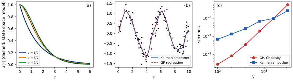
fig_S18_5. Download: PDF · SVG18.6 Learning the kernel
pp. 717–728 MacKay (1998) asked whether, in replacing neural networks by GPs, we had thrown the baby out with the bathwater: networks learn rich representations through adaptive hidden basis functions, whereas GPs with a fixed kernel such as the SE kernel are "just smoothing devices". The generalisation of a GP hinges on the kernel, so learning the kernel is how a GP does representation learning, and it is essential for extrapolation (Wilson and Adams, 2013). Learning a kernel resembles training a network, and the two combine in deep kernel learning (Section 18.6.6) and NN-GPs (Section 18.7).
18.6.1 Empirical Bayes for the kernel parameters
pp. 717–719, (18.161)–(18.165), Figures 18.15, 18.16 For 1-d regression with an SE kernel and observation noise, \(K_y(x_p,x_q)=\sigma_f^2\exp(-\frac1{2\ell^2}(x_p-x_q)^2)+\sigma_y^2\delta_{pq}\) (18.161): \(\ell\) is the horizontal scale, \(\sigma_f^2\) the vertical scale and \(\sigma_y^2\) the noise variance (the book's \(\ell\) in the figures is the same \(\ell\)). In Figure 18.15, 20 noisy points are drawn from a GP with \((\ell,\sigma_f,\sigma_y)=(1,1,0.1)\); the fit with these values is good (a), while \(\ell=3\), \(\sigma_y=0.89\) is smoother and underfits (b). Instead of a validation grid (as for SVMs) we maximise the marginal likelihood \[ \log p(\bm y\given\bm X,\bm\theta)=\log\N(\bm y\given\bm 0,\bm K_\sigma)=-\tfrac12\bm y^\T\bm K_\sigma^{-1}\bm y-\tfrac12\log|\bm K_\sigma|-\tfrac N2\log2\pi\tag{18.162--18.163}\] (the marginal is over the latent \(\bm f\)). For short length scales the fit term is small but \(\bm K\) is almost diagonal so \(\log|\bm K_\sigma|\) is large (complex); for long length scales the reverse (Gap 18.10). The gradient is \[ \frac{\partial}{\partial\theta_j}\log p(\bm y\given\bm X,\bm\theta)=\tfrac12\bm y^\T\bm K_\sigma^{-1}\frac{\partial\bm K_\sigma}{\partial\theta_j}\bm K_\sigma^{-1}\bm y-\tfrac12\Tr\Big(\bm K_\sigma^{-1}\frac{\partial\bm K_\sigma}{\partial\theta_j}\Big)=\tfrac12\Tr\Big((\bm\alpha\bm\alpha^\T-\bm K_\sigma^{-1})\frac{\partial\bm K_\sigma}{\partial\theta_j}\Big),\tag{18.164--18.165}\] \(\bm\alpha=\bm K_\sigma^{-1}\bm y\); cost \(O(N^3)\) for \(\bm K_\sigma^{-1}\) and \(O(N^2)\) per hyper-parameter. For positive parameters use \(\theta=\log\sigma_y^2\) and the chain rule. Any gradient optimiser applies, but the objective is not convex, so restarts are needed.
Filling the gap 18.22: the gradient of the marginal likelihood p. 718, (18.164)–(18.165)
Derivation
Write \(\bm K_\sigma=\bm K_\sigma(\bm\theta)\) and \(\partial_j=\partial/\partial\theta_j\). Differentiating \(\bm K_\sigma\bm K_\sigma^{-1}=\bm I\) gives \(\partial_j\bm K_\sigma^{-1}=-\bm K_\sigma^{-1}(\partial_j\bm K_\sigma)\bm K_\sigma^{-1}\). For the determinant, Jacobi's formula \(\partial_j\log|\bm K_\sigma|=\Tr(\bm K_\sigma^{-1}\partial_j\bm K_\sigma)\) (follows from \(\log|\bm K|=\sum\log\lambda_i\) and first-order perturbation of eigenvalues, or from the expansion \(|\bm K+\varepsilon\bm E|=|\bm K|\,|\bm I+\varepsilon\bm K^{-1}\bm E|=|\bm K|(1+\varepsilon\Tr\bm K^{-1}\bm E+O(\varepsilon^2))\)). Therefore, for \(\ell(\bm\theta)=-\frac12\bm y^\T\bm K_\sigma^{-1}\bm y-\frac12\log|\bm K_\sigma|-\frac N2\log2\pi\), \[ \partial_j\ell=\tfrac12\bm y^\T\bm K_\sigma^{-1}(\partial_j\bm K_\sigma)\bm K_\sigma^{-1}\bm y-\tfrac12\Tr(\bm K_\sigma^{-1}\partial_j\bm K_\sigma)\tag{18.164}\] and \(\bm y^\T\bm K_\sigma^{-1}\bm E\bm K_\sigma^{-1}\bm y=\bm\alpha^\T\bm E\bm\alpha=\Tr(\bm\alpha\bm\alpha^\T\bm E)\) gives (18.165). For the SE kernel with variance \(\sigma_f^2\), length scale \(\ell\) and noise \(\sigma_y^2\): \(\partial\bm K/\partial\ell=\bm K_f\circ(\bm r^2/\ell^3)\) (with \(r_{pq}=x_p-x_q\)), \(\partial\bm K/\partial\sigma_f=2\bm K_f/\sigma_f\), \(\partial\bm K_\sigma/\partial\log\sigma_y^2=\sigma_y^2\bm I\). I checked (18.164)–(18.165) against automatic differentiation for three log-parameters. Note that the gradient needs \(\bm K_\sigma^{-1}\) (or at least the trace) whereas the value needs only a Cholesky factor; trace estimators (Gap 18.19) avoid the cubic cost in iterative GP methods.
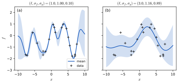
fig_18_15. Reproduces Murphy (2023), Figure 18.15. Download: PDF · SVG18.6.1.1 Example
p. 719, Figure 18.16 The marginal likelihood can have several local optima. With 7 data points (shown in panels b and c) and \(\sigma_f^2=1\), the log marginal likelihood against \((\ell,\sigma_y^2)\) has a low-noise, short-length-scale optimum (b) and a high-noise, long-length-scale optimum (c). With so little data there is no decisive evidence between them, though the more complex model (b) has a likelihood that is a good deal higher; with more data it would win clearly. In the region \(\sigma_y^2\approx1\) all variation is explained as noise and the likelihood does not depend on \(\ell\) (horizontal contours); for very short \(\ell\) the data are interpolated and the likelihood does not depend on the noise (vertical contours). A good optimiser would choose neither (limits in Gap 18.10). (The caption of the book's figure says "local minima": they are local maxima of the log marginal likelihood, minima of its negative.)
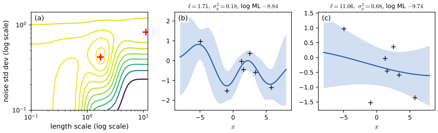
fig_18_16. Reproduces Murphy (2023), Figure 18.16. Download: PDF · SVGSee also: Introduction volume: GP marginal likelihood demonstration (Figures 17.8 and 17.9); Bayesian and Probabilistic ML, 6.4.3 learning the hyper-parameters.
18.6.2 Bayesian inference for the kernel parameters
pp. 720–721, (18.166), Figures 18.17, 18.18 With few data (e.g. in Bayesian optimisation, Section 6.6) a point estimate of \(\bm\theta\) can be badly overconfident: if the function values seen so far are all similar one may estimate \(\hat\sigma\approx0\). Instead compute a posterior over \(\bm\theta\) and average the predictions, \[ p(\bm f\given\mathcal D)=\sum_{s=1}^Sp(\bm f\given\mathcal D,\bm\theta_s)\,p(\bm\theta_s\given\mathcal D)\,w_s,\tag{18.166}\] with weights \(w_s\) for grid points. If \(\bm\theta\) is low-dimensional use a grid centred on the MAP; in higher dimensions a central composite design uses the mode and \(\pm1\) standard deviation along each axis, \(2|\bm\theta|+1\) points (Rue et al., 2009); or Monte Carlo: slice sampling, HMC (Section 12.5) or SMC. A conjugate prior on \(\sigma^2\) can be integrated out to give a Student-\(t\) process (a more robust GP).
Filling the gap 18.23: the hyper-parameter mixture (18.166) and why plug-in under-estimates uncertainty pp. 720–721
Derivation
By the sum rule, \(p(\bm f_*\given\mathcal D)=\int p(\bm f_*\given\mathcal D,\bm\theta)p(\bm\theta\given\mathcal D)\d\bm\theta\), and approximating the integral by a weighted sum over \(\bm\theta_s\) gives (18.166); for a grid, \(w_s\propto\) the volume of the cell, and the weights \(p(\bm\theta_s\given\mathcal D)\propto p(\mathcal D\given\bm\theta_s)p(\bm\theta_s)\) are normalised to sum to one. The predictive is a mixture of Gaussians, not a Gaussian: with component means \(\mu_s(\bm x)\) and variances \(v_s(\bm x)\) and normalised weights \(\pi_s\), the law of total variance gives \[ \E[f(\bm x)\given\mathcal D]=\sum_s\pi_s\mu_s(\bm x),\qquad\var[f(\bm x)\given\mathcal D]=\sum_s\pi_sv_s(\bm x)+\sum_s\pi_s(\mu_s(\bm x)-\bar\mu(\bm x))^2 .\] The second term, the variance of the posterior mean across hyper-parameters, is exactly the extra uncertainty that the plug-in \(p(\bm f\given\mathcal D,\hat{\bm\theta})\) omits: the plug-in uses only the first term at one \(\bm\theta\), and so is overconfident when the posterior of \(\bm\theta\) is wide. This is the effect in Figure 18.18: beyond the data the hyper-parameter posterior is spread over very different periods and length scales, so the mixture's variance is much larger than that of any component. The central-composite weights approximate the integral by a Gaussian quadrature over the Laplace approximation of \(p(\bm\theta\given\mathcal D)\) (Rue et al., 2009).
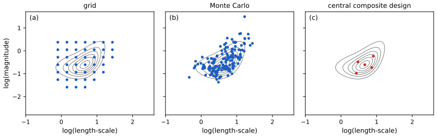
fig_18_17. Reproduces Murphy (2023), Figure 18.17. Download: PDF · SVG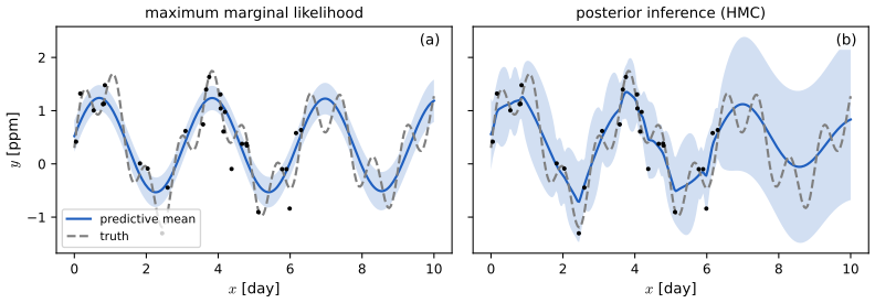
fig_18_18. Reproduces Murphy (2023), Figure 18.18. Download: PDF · SVG18.6.3 Multiple kernel learning for additive kernels
pp. 721–722, (18.168)–(18.171), Figures 18.19, 18.20 A sum of \(B\) base kernels \(K=\sum_bw_bK_b\) (18.168) with weights \(w_b>0\) estimated by structural risk minimisation is multiple kernel learning (Rakotomamonjy et al., 2008). If each base kernel depends on a subset of the variables with a hierarchical inclusion property (\(k_{123}\) implies \(k_{12},k_{13},k_{23}\)) one has hierarchical kernel learning (Bach, 2009; convex, but with cross-validation for the weights; a more efficient empirical-Bayes version is in Duvenaud et al. 2011), Figure 18.19. The usual restriction is to first-order additive kernels \(K=\sum_dK_d(x_d,x_d')\) (18.169), whose functions are \(f(\bm x)=f_1(x_1)+\cdots+f_D(x_D)\) (18.170): a generalised additive model (GAM). Duvenaud et al. also take a weighted sum of additive kernels of every order. Dong et al. (2020) show that additive kernels on different 1-d projections \(K=\sum_bw_bK_b(\bm P_b\bm x,\bm P_b\bm x')\) (18.171) can match full-input kernels even when the projections are not learned, and the orthogonal additive kernel (OAK; Lu et al., 2022) imposes orthogonality for identifiability. In Figure 18.20 each base kernel is \(\sigma_d^2\mathrm{SE}(x_d,x_d'\given\ell_d)\), and the amplitudes of irrelevant inputs go to zero. Because the model is additive, the posterior mean of each component is a separate function (computed from \(\bm K_d\bm\alpha\) with the full \(\bm\alpha\)); the component means sum to the overall posterior mean (checked).
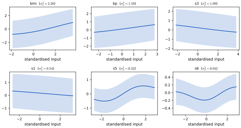
fig_18_20. Reproduces Murphy (2023), Figure 18.20. Download: PDF · SVG18.6.4 Automatic search for compositional kernels
pp. 722–725, Figures 18.21, 18.22 The methods above fit hyper-parameters of a given family but do not choose the kernel. The search of Duvenaud et al. (2013) explores increasingly complex kernel expressions: start from white noise, replace a kernel by a sum \(k\to k+k'\) or a product \(k\to k\times k'\) with a base kernel \(k'\in\{\mathrm{SE},\mathrm{RQ},\mathrm{Lin},\mathrm{Per},\dots\}\), fit each candidate, and keep the one with the best BIC, \(\mathrm{BIC}(m)=\log p(\mathcal D\given m)-\frac12|m|\log N\) (Section 3.8; \(p(\mathcal D\given m)\) is the marginal likelihood at the fitted parameters and \(|m|\) the number of parameters). It resembles what a human expert does: look for structure in the residual (periodicity), start from a global linear trend that turns out to hold only locally and multiply it by an SE kernel, add input dimensions one at a time. The result can be turned into a natural-language description (Lloyd et al., 2014). Sun et al. (2018) show how to build a differentiable network of sums and products of kernels, much faster to train. On the monthly airline passenger data (Figure 18.22) the search found a summary with four trends in the book: a linear trend, a roughly periodic yearly function with linearly growing amplitude, a smooth function, and uncorrelated noise with linearly increasing standard deviation.
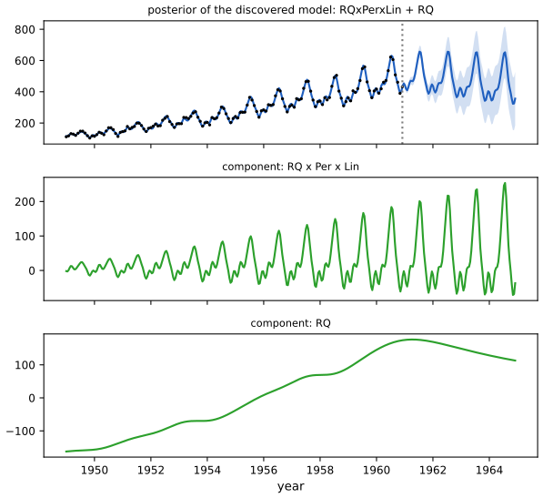
fig_18_22. Reproduces Murphy (2023), Figure 18.22. Download: PDF · SVG18.6.5 Spectral mixture kernel learning
pp. 725–726, (18.172), Figures 18.23, 18.24 Since any stationary kernel is the Fourier transform of a spectral density (18.22), learning the density is equivalent to learning the kernel. Additive combinations of SE and Matérn kernels with different length scales amount to a scale mixture of Gaussians or Student laws centred at the origin, which is a very inflexible density model; a scale-location mixture of Gaussians is far more flexible and gives the spectral mixture kernel \[ K(x,x')=\sum_iw_i\cos\big((x-x')2\pi\mu_i\big)\exp\big(-2\pi^2(x-x')^2v_i\big),\tag{18.172}\] whose weights, means and variances can be learned by empirical Bayes (Section 18.6.1) or fully Bayesian inference (Jang et al., 2017); derivation in Gap 18.2. Learning it enables extrapolation (Figure 18.24, which compares Matérn, RQ, periodic, SE and spectral mixture kernels, all learned by empirical Bayes, on CO2 and airline data; compare the hand-built kernel of Section 18.8.1). Scalable inference that preserves structure (Kronecker methods, KISS-GP, conjugate gradients) is needed for large spatio-temporal problems.
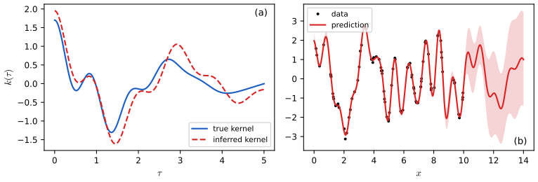
fig_18_23. Reproduces Murphy (2023), Figure 18.23. Download: PDF · SVG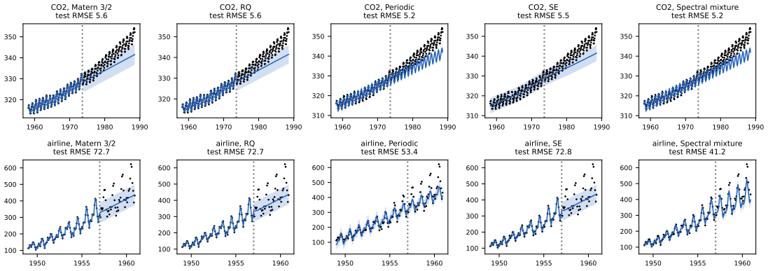
fig_18_24. Reproduces Murphy (2023), Figure 18.24. Download: PDF · SVG18.6.6 Deep kernel learning
pp. 726–728, (18.173), Figures 18.25–18.27 Deep kernel learning (Salakhutdinov and Hinton, 2007; Wilson et al., 2016) combines a network's structure with a GP's non-parametric flexibility and uncertainty. A deep RBF kernel is \[ K_\theta(\bm x,\bm x')=\exp\!\Big(-\frac1{2\sigma^2}\|\bm h^L_\theta(\bm x)-\bm h^L_\theta(\bm x')\|^2\Big),\tag{18.173}\] with \(\bm h^L_\theta\) the output of layer \(L\) of a network (Figure 18.25), and \(\theta\) learned by maximising the GP marginal likelihood. The network can be pre-trained, learned jointly with the base-kernel parameters, or pre-trained then fine-tuned. It is a "last-layer" Bayesian model: the base kernel measures distance in feature space, keeping uncertainty high far from the data. It lets a GP fit discontinuities (Figure 18.26): an MLP maps the input through a smooth warp that makes the base kernel see a sharp change. Figure 18.27 (not reproduced) shows that a deep kernel learns a diagonal band for face orientation where a plain RBF kernel stays diffuse. Ober et al. (2021) show that marginal-likelihood training of a deep kernel can overfit worse than ordinary network training, and propose fully Bayesian inference over weights and hyper-parameters with SGLD.
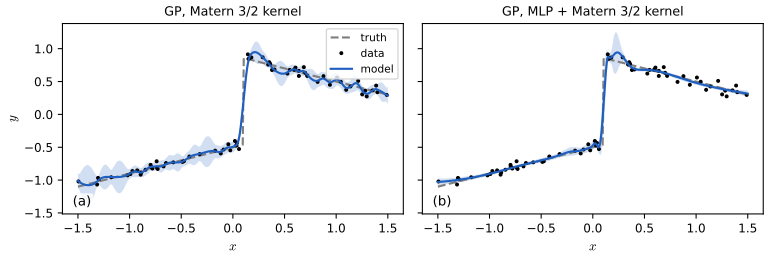
fig_18_26. Reproduces Murphy (2023), Figure 18.26. Download: PDF · SVG18.7 GPs and DNNs
p. 728 Section 18.6.6 put a network inside a GP. In the other direction, infinitely wide networks are GPs with particular fixed kernels (Section 18.7.1), gradient descent on a wide network behaves like kernel regression with a different kernel, the neural tangent kernel (Section 18.7.2), and a hierarchy of GPs is a deep GP (Section 18.7.3).
18.7.1 Kernels derived from infinitely wide DNNs (NN-GP)
pp. 729–730, (18.174)–(18.183), Table 18.4, Figure 18.28 Consider a one-hidden-layer MLP with \(H\) hidden units and activation \(\varphi\), \[ f_k(\bm x)=b_k+\sum_{j=1}^Hv_{jk}h_j(\bm x),\qquad h_j(\bm x)=\varphi(u_{0j}+\bm x^\T\bm u_j),\tag{18.174}\] with independent Gaussian priors \(b_k\sim\N(0,\sigma_b^2)\), \(v_{jk}\sim\N(0,\sigma_v^2)\), \(u_{0j}\sim\N(0,\sigma_0^2)\), \(\bm u_j\sim\N(\bm0,\bm\Sigma)\) (18.175). The mean is zero (18.176) and the covariance of one output at two inputs is \(\sigma_b^2+\sigma_v^2H\,\E_u[h(\bm x)h(\bm x')]\) (18.177)–(18.178). With \(\sigma_v^2=\omega/H\), as \(H\to\infty\) the sum over hidden units converges (central limit theorem) to a Gaussian, jointly over any finite set of inputs, with \[ \E[f_k(\bm x)f_k(\bm x')]=\sigma_b^2+\omega\,\E_u[h(\bm x)h(\bm x')]\triangleq K(\bm x,\bm x'),\tag{18.179--18.180}\] so the MLP converges to a GP with kernel \(K\), the NN-GP kernel (Neal, 1996; Williams, 1998; extended to deep MLPs, CNNs and general architectures by Lee et al., 2018; Novak et al., 2019; Yang, 2019). With \(\tilde{\bm x}=(1,\bm x)\), \(\tilde{\bm u}=(u_0,\bm u)\), \(\tilde{\bm\Sigma}=\diag(\sigma_0^2,\bm\Sigma)\), \[ C(\bm x,\bm x')=\E_u[h(\tilde{\bm u}^\T\tilde{\bm x})h(\tilde{\bm u}^\T\tilde{\bm x}')]=\int h(\tilde{\bm u}^\T\tilde{\bm x})h(\tilde{\bm u}^\T\tilde{\bm x}')\N(\tilde{\bm u}\given\bm0,\tilde{\bm\Sigma})\d\tilde{\bm u},\tag{18.181--18.183}\] available in closed form for some activations (Table 18.4). It is non-stationary; samples are nearly discontinuous and tend to constants for large \(|x|\) (Figure 18.28). The NN-GP kernel is fixed, so there is no representation learning, as opposed to a finite network.
Filling the gap 18.24: the NN-GP limit, and the kernels of erf, Heaviside and ReLU units (Table 18.4) pp. 729–730, (18.177)–(18.183), Table 18.4
Derivation
Why the limit is Gaussian. Condition on the first-layer weights. Then \(h_j(\bm x)\) are fixed numbers, and \(f_k(\bm x)=b_k+\sum_jv_{jk}h_j(\bm x)\) is a linear function of independent Gaussians, hence exactly Gaussian jointly over any finite set of inputs, with mean 0 and covariance \(K_H(\bm x,\bm x')=\sigma_b^2+\frac\omega H\sum_{j=1}^Hh_j(\bm x)h_j(\bm x')\). The \(h_j(\bm x)h_j(\bm x')\) are iid over \(j\) (the first-layer weights of different units are independent) with mean \(C(\bm x,\bm x')\), so by the law of large numbers \(K_H\to\sigma_b^2+\omega C=K\) almost surely (if \(\E[h^2]<\infty\)). A Gaussian vector with covariance converging a.s. has characteristic function converging a.s., and by dominated convergence the characteristic function of the unconditional law converges to that of \(\N(\bm 0,K)\). So every finite-dimensional distribution is Gaussian in the limit: a GP. (This conditional route needs only the law of large numbers; the book's central-limit argument over the sum \(\sum_jv_{jk}h_j\) reaches the same conclusion but requires checking the Lindeberg condition.) The error \(K_H-K\) is \(O(H^{-1/2})\): Figure 18.S3b shows the maximum error of the empirical kernel against the closed forms falling with slope \(-\tfrac12\).
Closed forms. Let \(\bm u\sim\N(\bm0,\bm\Sigma)\) and write \(a=\bm u^\T\bm x\), \(b=\bm u^\T\bm x'\) (for the augmented vectors): \((a,b)\) is bivariate Gaussian with covariance \(\begin{pmatrix}\bm x^\T\bm\Sigma\bm x&\bm x^\T\bm\Sigma\bm x'\\\cdot&\bm x'^\T\bm\Sigma\bm x'\end{pmatrix}\). Let \(\theta\) be the angle between \(\bm\Sigma^{1/2}\bm x\) and \(\bm\Sigma^{1/2}\bm x'\) (\(\cos\theta=\bm x^\T\bm\Sigma\bm x'/\sqrt{\bm x^\T\bm\Sigma\bm x\;\bm x'^\T\bm\Sigma\bm x'}\)).
- Heaviside, \(h=\mathbb 1[\cdot\ge0]\): the probability that two correlated Gaussians are both positive is the orthant probability \(\frac12-\frac\theta{2\pi}=\frac{\pi-\theta}{2\pi}\).
- ReLU, \(h=\max(0,\cdot)\): rotate so that \(\bm\Sigma^{1/2}\bm x=|\bm x|_\Sigma(1,0)\) and \(\bm\Sigma^{1/2}\bm x'=|\bm x'|_\Sigma(\cos\theta,\sin\theta)\) and use polar coordinates for the standard normal \(\bm w=\rho(\cos\varphi,\sin\varphi)\), \(\E\rho^2=2\): \(\E[\mathrm{ReLU}(a)\mathrm{ReLU}(b)]=|\bm x|_\Sigma|\bm x'|_\Sigma\,2\cdot\frac1{2\pi}\int_{\theta-\pi/2}^{\pi/2}\cos\varphi\cos(\varphi-\theta)\d\varphi\). The integral is \(\frac12\int[\cos(2\varphi-\theta)+\cos\theta]\d\varphi=\frac12[\sin\theta+(\pi-\theta)\cos\theta]\). Hence \(C=\dfrac{|\bm x|_\Sigma|\bm x'|_\Sigma}{2\pi}\big(\sin\theta+(\pi-\theta)\cos\theta\big)\) (the arc-cosine kernel of order 1; Cho and Saul, 2009).
- erf (Williams, 1998): \(\mathrm{erf}(z)=2\Phi(\sqrt2z)-1=\E_\xi\,\mathrm{sign}(\sqrt2z+\xi)\) with \(\xi\sim\N(0,1)\). So \(\E[\mathrm{erf}(a)\mathrm{erf}(b)]=\E\,\mathrm{sign}(X)\mathrm{sign}(Y)\) with \((X,Y)=(\sqrt2a+\xi,\sqrt2b+\xi')\) Gaussian with covariance \(\begin{pmatrix}1+2\bm x^\T\bm\Sigma\bm x&2\bm x^\T\bm\Sigma\bm x'\\\cdot&1+2\bm x'^\T\bm\Sigma\bm x'\end{pmatrix}\). For correlated standard Gaussians, \(\E\,\mathrm{sign}X\,\mathrm{sign}Y=1-2\frac{\arccos\rho}\pi=\frac2\pi\arcsin\rho\) (twice the orthant probability, minus one). Therefore \(C=\frac2\pi\arcsin\!\big(\frac{2\bm x^\T\bm\Sigma\bm x'}{\sqrt{(1+2\bm x^\T\bm\Sigma\bm x)(1+2\bm x'^\T\bm\Sigma\bm x')}}\big)\), the first row of Table 18.4.
I confirmed all three by Monte Carlo (\(2\times10^6\) draws; the erf kernel to \(3\times10^{-4}\)). On the printed table. With \(u\sim\N(\bm0,\tilde{\bm\Sigma})\) the Heaviside entry is \((\pi-\theta)/(2\pi)\), not \(\pi-\theta\), and the ReLU entry is \(\frac1{2\pi}(\ldots)\); the table's ReLU entry \(\frac{f_2}\pi\sin\theta+\frac{\pi-\theta}\pi\tilde{\bm x}^\T\tilde{\bm\Sigma}\tilde{\bm x}'\) equals twice the expectation (and its Heaviside entry equals \(2\pi\) times it), i.e. it is defined up to a positive constant that is absorbed by the output variance \(\omega\); only the erf row is exactly the expectation.
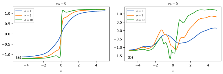
fig_18_28. Reproduces Murphy (2023), Figure 18.28. Download: PDF · SVG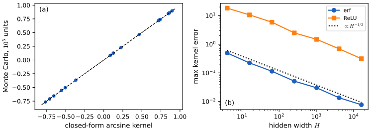
fig_S18_3. Download: PDF · SVG18.7.2 Neural tangent kernel (NTK)
p. 731, (18.184)–(18.187), Figure 18.S4 (extra) The NN-GP kernel describes the network at random initialisation. Can a kernel describe it during training? With predictions \(\bm f=[f(\bm x_n;\bm\theta)]_n\), loss gradient \(\nabla_{\bm f}L\), parameters \(\bm\theta\in\R^P\) and the \(P\times N\) Jacobian \(\nabla_{\bm\theta}\bm f\), gradient descent in continuous time with learning rate \(\eta\) obeys \(\partial_t\bm\theta_t=-\eta\nabla_{\bm\theta}L=-\eta\nabla_{\bm\theta}\bm f_t\,\nabla_{\bm f}L(\bm f_t)\) (18.184), so the function evolves as \[ \partial_t\bm f_t=\nabla_{\bm\theta}\bm f_t^\T\partial_t\bm\theta_t=-\eta\,\bm T_t\,\nabla_{\bm f}L(\bm f_t),\qquad\bm T_t(\bm x,\bm x')=\nabla_{\bm\theta}f_t(\bm x)\cdot\nabla_{\bm\theta}f_t(\bm x')=\sum_{p=1}^P\frac{\partial f(\bm x;\bm\theta)}{\partial\theta_p}\frac{\partial f(\bm x';\bm\theta)}{\partial\theta_p}\Big|_{\bm\theta_t}.\tag{18.185--18.186}\] As \(\eta\to0\) and the widths \(\to\infty\) this kernel converges to a constant kernel, the neural tangent kernel \(\mathcal T(\bm x,\bm x')=\nabla_{\bm\theta}f(\bm x;\bm\theta_\infty)\cdot\nabla_{\bm\theta}f(\bm x';\bm\theta_\infty)\) (18.187) (Jacot et al., 2018; for CNNs, graph nets and general architectures, Arora et al., 2019; Du et al., 2019; Yang, 2019). The parameters then barely move from their initial values (so a linear approximation about the start is valid) yet the predictions can change completely and reach zero training error, because the last layer learns to use the random features as in kernel regression: "lazy training" (Chizat et al.). It is not representative of practical networks, whose parameters move a lot (Woodworth et al.); other parametrisations keep feature learning in the infinite-width limit (Yang and Hu, 2021).
Filling the gap 18.25: the NTK: function-space dynamics, the linearised solution and how it is a kernel regression p. 731, (18.184)–(18.187)
Derivation
(18.185). Chain rule: \(\partial_tf_t(\bm x_n)=\sum_p\partial_{\theta_p}f(\bm x_n)\,\partial_t\theta_p\) and \(\partial_t\theta_p=-\eta\sum_m\partial_{\theta_p}f(\bm x_m)\,\partial_{f_m}L\), so \(\partial_tf_t(\bm x_n)=-\eta\sum_m\big[\sum_p\partial_{\theta_p}f(\bm x_n)\partial_{\theta_p}f(\bm x_m)\big]\partial_{f_m}L=-\eta\sum_mT_t(\bm x_n,\bm x_m)\partial_{f_m}L\). The same holds for a test input \(\bm x_*\) with \(\bm T_t(\bm x_*,\bm X)\). The kernel \(\bm T_t\) is a Gram matrix of gradient vectors, hence positive semi-definite, so \(\partial_tL=\nabla_{\bm f}L^\T\partial_t\bm f=-\eta\nabla_{\bm f}L^\T\bm T_t\nabla_{\bm f}L\le0\): the loss decreases along the flow. I checked the one-step identity \(\bm f_{t+1}-\bm f_t=-\eta\bm T_t(\bm f_t-\bm y)\) to \(O(\eta^2)\) on a width-200 network.
Constant-kernel solution. Take \(L=\tfrac12\|\bm f-\bm y\|^2\), so \(\nabla_{\bm f}L=\bm f-\bm y\), and suppose \(\bm T_t\equiv\bm T\) is constant (the NTK regime). The ODE on the training set is linear, \(\partial_t(\bm f_t-\bm y)=-\eta\bm T(\bm f_t-\bm y)\), with solution \(\bm f_t(\bm X)-\bm y=e^{-\eta\bm Tt}(\bm f_0(\bm X)-\bm y)\): each eigen-direction of \(\bm T\) decays at the rate \(\eta\lambda_i(\bm T)\), so directions with large eigenvalues are learned first. For a test input, \(\partial_tf_t(\bm x_*)=-\eta\bm T_{*,X}(\bm f_t(\bm X)-\bm y)\) integrates to \[ f_t(\bm x_*)=f_0(\bm x_*)-\bm T_{*,X}\bm T^{-1}\big(\bm I-e^{-\eta\bm Tt}\big)(\bm f_0(\bm X)-\bm y)\ \xrightarrow{t\to\infty}\ f_0(\bm x_*)+\bm T_{*,X}\bm T^{-1}(\bm y-\bm f_0(\bm X)),\] which is kernel regression with the NTK (interpolation) applied to the residual of the initial network. If \(\bm f_0\) is drawn from the NN-GP, \(f_\infty\) is a GP draw conditioned (in the kernel sense) on the data. Why the kernel is constant. At initialisation, \(\bm T_0(\bm x,\bm x')\) is a sum over parameters of products of derivatives, each of order \(1/m\) in the NTK parametrisation \(f=m^{-1/2}\sum_ja_j\mathrm{relu}(w_jx+b_j)\), so by the law of large numbers it converges to a deterministic kernel; the harder part of the theorem is that \(\bm T_t\) stays close to \(\bm T_0\) because each parameter moves by \(O(m^{-1/2})\) while the function moves by \(O(1)\) (summed over \(m\) parameters). I do not prove that here (see Jacot et al. 2018). Numerically (Figure 18.S4) with \(m=8,\dots,8192\): the relative drift \(\|\bm T_{\rm end}-\bm T_0\|/\|\bm T_0\|\) falls from 1.2 to 0.012, roughly like \(m^{-1/2}\), the distance between the trained network and the linearised dynamics falls similarly, and the change in the function from its initial value stays \(O(1)\): lazy training.
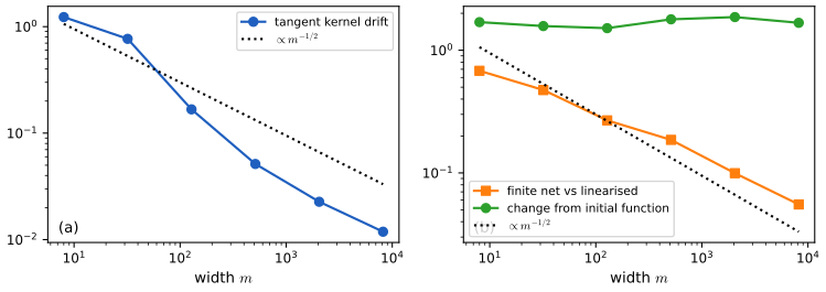
fig_S18_4. Download: PDF · SVG18.7.3 Deep GPs
pp. 731–732, (18.188) A deep Gaussian process (DGP; Damianou and Lawrence, 2013) is a composition of GPs, \(\mathrm{DGP}(\bm x)=f_L\circ\cdots\circ f_1(\bm x)\) with \(f_i=[f_i^{(1)},\dots,f_i^{(H_i)}]\) and \(f_i^{(j)}\sim\GP(0,K_i)\) (18.188): the hidden nodes of a deep network become hidden functions. A single-layer GP is non-parametric and can model any function with a non-degenerate kernel and enough data, but its performance is limited by the choice of kernel. A GP on top of a network (deep kernel learning) is still just a GP; a composition of GPs is strictly more general. Inference in DGPs is complicated; it is described in Supplementary Section 18.1, which is in Section S18.1 below (Jakkala, 2021, is a recent survey).
18.8 Gaussian processes for time series forecasting
p. 732 To forecast a series, model the unknown value as a function of time \(f(t)\), put a GP prior on \(f\), update it with the observed series and extrapolate. A naive implementation costs \(O(T^3)\); for stationary kernels with a rational spectrum (Matérn exactly, SE approximately) the problem can be written as a linear-Gaussian state space model and solved by a Kalman smoother in \(O(T)\) (Särkkä, Solin and Hartikainen, 2013; Särkkä and Solin, 2019; Section 18.5.6, Gap 18.21), or \(O(\log T)\) span with a parallel prefix scan on a GPU (Section 8.2.3).
18.8.1 Example: Mauna Loa
pp. 732–733, (18.189)–(18.193), Figure 18.29 Figure 18.29a shows the Mauna Loa CO2 record: a year-long (quasi-)periodic signal on a long-term trend. Following Rasmussen and Williams (Section 5.4.3), the kernel is a sum of four parts, \[ K(r)=K_1(r)+K_2(r)+K_3(r)+K_4(r),\tag{18.189}\] \[ K_1=\theta_0^2\exp\!\Big(-\frac{r^2}{2\theta_1^2}\Big),\quad K_2=\theta_2^2\exp\!\Big(-\frac{r^2}{2\theta_3^2}-\theta_5\sin^2\frac{\pi r}{\theta_4}\Big),\quad K_3=\theta_6^2\Big(1+\frac{r^2}{2\theta_8\theta_7^2}\Big)^{-\theta_8},\quad K_4=\theta_9^2\exp\!\Big(-\frac{r^2}{2\theta_{10}^2}\Big).\tag{18.190--18.193}\] \(K_1\) is the smooth long-term trend (amplitude \(\theta_0\), length scale \(\theta_1\)); \(K_2\) the seasonal cycle: a periodic kernel with period \(\theta_4\) (about one year) multiplied by an SE kernel with decay time \(\theta_3\) so that the cycle may slowly change, with smoothness \(\theta_5\); \(K_3\) a rational quadratic for medium-term irregularities (magnitude \(\theta_6\), length \(\theta_7\), shape \(\theta_8\)); \(K_4\) an SE kernel for correlated noise (the independent noise is part of the likelihood). The combination of \(K_1\) and \(K_4\) is non-identifiable: the two SE parts can be exchanged with the same likelihood, which does not affect predictions. All parameters are fitted by maximising the marginal likelihood (Section 18.6.1), and the model forecasts the series (Figure 18.29b).
My reproduction uses the monthly means of the 1958–2001 record (521 months), training on the 377 months before 1990 and forecasting the remaining 144 months. The fitted parameters are \(\theta=(57.4,\ 55.0,\ 3.38,\ 151.7,\ 1.00,\ 0.75,\ 0.34,\ 0.78,\ 12.7,\ 0.19,\ 0.12)\) with noise standard deviation 0.20 ppm, and the log marginal likelihood is \(-88.4\). The period comes out at 1.000 years, a decay time of 152 years makes the seasonal cycle almost exactly periodic, and the forecast has an RMSE of 2.2 ppm on the held-out 1990–2001 months. Removing a part shows what each does: without \(K_2\) the log marginal likelihood falls to \(-5753\) (all the seasonal swing is unexplained), without \(K_1\) to \(-1923\), without \(K_3\) to \(-165\) and without \(K_4\) to \(-130\) (parameters held at their fitted values); with only \(K_1\) it is \(-19799\).
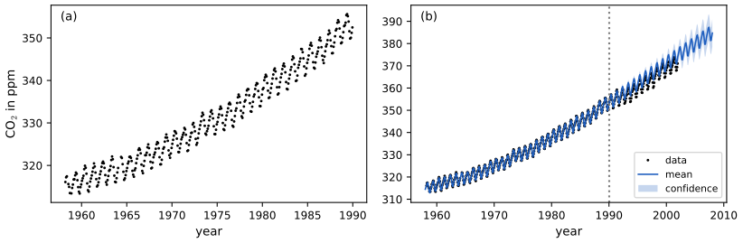
fig_18_29. Reproduces Murphy (2023), Figure 18.29. Download: PDF · SVGSupplement S18 (supplementary Chapter 18: deep GPs and GPs as state space models)
The supplement has two sections. The second (GPs and state space models) fills in the matrices quoted at the end of Section 18.5.6 and is treated there (Gap 18.21).
S18.1 Deep GPs
supplement pp. 183–188 A deep GP is \(f_L\circ\cdots\circ f_1\) with each layer a (multi-output) GP (S18.1); a single-layer GP is limited by its kernel, which a DGP can partly overcome (S18.1.0.2); posterior inference is hard (S18.1.0.3); an infinitely wide DGP behaves like a single-layer GP (S18.1.0.4); and BNNs are degenerate DGPs (S18.1.0.5).
S18.1.0.1 Construction of a deep GP
supplement pp. 183–184, (S18.2), Supplement Figure 18.1 A two-layer example following Pleiss and Cunningham (2021): \(f_1^{(j)}\sim\GP(0,K_1)\), \(j=1{:}H_1\), \(f_2\sim\GP(0,K_2)\). With training data \((\bm X,\bm y)\), define \(\bm F_1=[f_1(\bm x_1),\dots,f_1(\bm x_N)]\), \(\bm f_2=[f_2(f_1(\bm x_n))]_n\), and for a test input \(\bm x_*\), \(\bm f_1^*=f_1(\bm x_*)\), \(f_2^*=f_2(f_1(\bm x_*))\). The joint is \(p(f_2^*,\bm f_2,\bm F_1,\bm f_1^*,\bm y)=p(f_2^*\given\bm f_2,\bm f_1^*,\bm F_1)p(\bm f_2\given\bm F_1,\bm f_1^*)p(\bm f_1^*,\bm F_1)p(\bm y\given\bm f_2)\) with kernel matrices \(\bm K_2=K_2(\bm F_1,\bm F_1)\), \(\bm k_2^*=K_2(\bm F_1,\bm f_1^*)\), \(k_2^{**}=K_2(\bm f_1^*,\bm f_1^*)\) (Supplement Figure 18.1, a graphical model). Note that the layer-2 kernel is evaluated on the random hidden values, so it is itself random.
S18.1.0.2 Example: 1d step function
supplement pp. 183–185, Figures S18.2, S18.3 Data from a step function arise when a physical process saturates. A GP with an RBF kernel over-smooths and does not pick up the discontinuity (Supplement Figure 18.2a); one can warp the input with a learned network (Figure 18.26) or compose smooth maps. A four-layer DGP with one hidden unit per layer and RBF kernels (\(K_1=\exp(-\|x-x'\|^2/2D)\), \(K_2=\exp(-\|f_1-f_1'\|^2/2H_1)\), etc.) fits the step (Supplement Figure 18.2b), and the predictions away from the data show two plausible modes (the signal continues at 0 or at 1): the posterior mean is a poor summary of such a predictive distribution. The functions learned at each layer are individually smooth, but their composition is not (Supplement Figure 18.3).
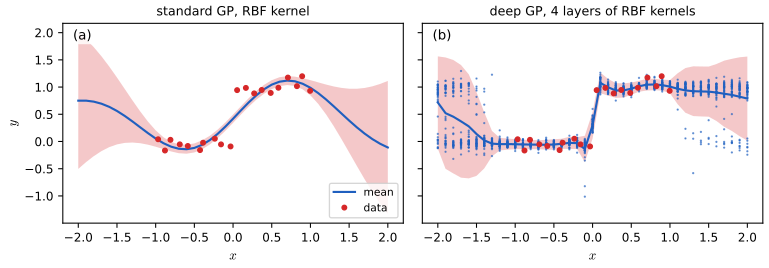
fig_sup18_2. Reproduces Murphy (2023), Supplement Figure 18.2. Download: PDF · SVG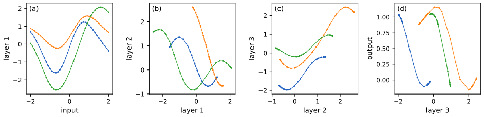
fig_sup18_3. Reproduces Murphy (2023), Supplement Figure 18.3. Download: PDF · SVGS18.1.0.3 Posterior inference
supplement pp. 185–186, (S18.3)–(S18.10) Conditioning the two-layer joint on \(\bm y\) and using the conditional independences of Supplement Figure 18.1, \[ p(f_2^*,\bm f_2,\bm F_1,\bm f_1^*\given\bm y)=p(f_2^*\given\bm f_2,\bm f_1^*,\bm F_1)p(\bm f_2\given\bm F_1,\bm y)p(\bm f_1^*,\bm F_1\given\bm y)=p(f_2^*\given\bm f_2,\bm K_2,\bm k_2^*,k_2^{**})p(\bm f_2\given\bm K_2,\bm y)p(\bm K_2,\bm k_2^*,k_2^{**}\given\bm y),\tag{S18.3--S18.6}\] because \(\bm f_2,f_2^*\) depend on \(\bm F_1,\bm f_1^*\) only through the kernel matrices, with \(f_2^*\given\bm f_2\sim\N((\bm k_2^*)^\T\bm K_2^{-1}\bm f_2,\,k_2^{**}-(\bm k_2^*)^\T\bm K_2^{-1}\bm k_2^*)\) (S18.5). The posterior mean is \[ \E[f_2^*\given\bm y]=\E_{\bm K_2,\bm k_2^*\given\bm y}\big[(\bm k_2^*)^\T\bm K_2^{-1}\E[\bm f_2\given\bm K_2,\bm y]\big]=\E_{f_1(\bm x_*),f_1(\bm x_1),\dots\given\bm y}\Big[\sum_{i=1}^N\alpha_iK_2(f_1(\bm x_i),f_1(\bm x_*))\Big],\tag{S18.7--S18.10}\] so inference marginalises over all hidden function values at every layer and every data point, which is expensive. Salimbeni and Deisenroth (2017) use the sparse variational method of Section 18.5.4 with inducing points at each layer (dependence between layers is exact); Dutordoir et al. (2021) show that the posterior mean of such a sparse variational approximation can be computed by a forward pass through a ReLU network. My figures do inference differently, by Hamiltonian Monte Carlo on the whitened hidden values (\(\bm F_l=\mathrm{chol}(\bm K_l(\bm F_{l-1}))\bm z_l\)) with the last layer integrated out exactly, for the 20 training and 41 test inputs jointly; this is a reliable but small-scale inference scheme (the 4-layer chain has acceptance 0.69).
S18.1.0.4 Behaviour in the limit of infinite width
supplement pp. 186–187, (S18.11), Supplement Figure 18.4 The posterior mean (S18.10) is a mixture of data-dependent kernel functions, since \(\bm K_2\) and \(\bm k_2^*\) depend on \(\bm y\) through the posterior of \(\bm F_1\): this is why a DGP is more expressive than a one-layer GP, whose kernel is fixed. But Pleiss and Cunningham (2021) show that as \(H_1\to\infty\) the posterior over the layer-2 kernel becomes independent of the data, \(p(\bm K_2,\bm k_2^*\given\bm y)=\delta(\bm K_2-\bm K_{\lim})\delta(\bm k_2^*-\bm k_{\lim}^*)\) with \(\bm K_{\lim}=\E[\bm f_2\bm f_2^\T]\) (expectation over the prior, depending on \(\bm X\) but not on \(\bm y\)), so \[ \lim_{H_1\to\infty}\E[f_2^*\given\bm y]=\sum_{i=1}^N\alpha_iK_{\lim}(\bm x_i,\bm x_*),\tag{S18.11}\] the form of a single-layer GP. For RBF kernels the limit is \(K_{\lim}(\bm x,\bm x')=\exp\big(\exp(-\|\bm x-\bm x'\|^2/2D)-1\big)\), which is stationary. In Supplement Figure 18.4 the width 1 DGP has a non-stationary covariance (long-range correlation near \(x=\pm1\), where the function is flat, short-range near 0 where it jumps), and as the width grows the average posterior covariance becomes stationary (constant diagonals). Increasing width also makes the marginals more Gaussian (central-limit behaviour) whereas increasing depth makes them less Gaussian (sharper peaks, heavier tails): hence deep but narrow DGPs work best.
Filling the gap 18.26: the infinite-width limit of a deep GP, and a proof that the posterior of the layer-2 kernel concentrates supplement pp. 186–187, (S18.11)
Derivation
The limit kernel. Let \(f_1^{(1)},\dots,f_1^{(H)}\) be iid \(\GP(0,K_1)\) with \(K_1(x,x)=1\) and \(K_2(\bm f,\bm f')=\exp(-\|\bm f-\bm f'\|^2/(2H))\) on \(\R^H\). For fixed inputs, \(\|\bm f(x)-\bm f(x')\|^2/H=\frac1H\sum_{h=1}^H(f^{(h)}(x)-f^{(h)}(x'))^2\) is an average of iid terms with mean \(\E(f(x)-f(x'))^2=K_1(x,x)+K_1(x',x')-2K_1(x,x')=2(1-K_1(x,x'))\). By the strong law of large numbers and continuity of \(\exp\), \[ K_2(\bm f_1(x),\bm f_1(x'))\xrightarrow{\rm a.s.}\exp\!\big(-(1-K_1(x,x'))\big)=\exp\big(K_1(x,x')-1\big),\qquad K_1=e^{-\|x-x'\|^2/2D}.\] This is \(K_{\lim}\) of (S18.11). It is a positive definite stationary kernel: \(\exp(K_1)\) is a kernel by the exponential rule (Gap 18.4) and multiplying by the constant \(e^{-1}\) preserves this. By the delta method the fluctuation of \(K_2\) around its limit is \(O(H^{-1/2})\): in simulation the standard deviation at \(r=1.1\) falls by a factor 3.98 from \(H=256\) to \(H=4096\) (4 expected), and the mean is \(0.7257,0.6358,0.6352\) for \(H=1,256,4096\) against the limit \(0.6351\).
Posterior concentration. The likelihood of the data depends on the hidden values \(\bm F_1\) only through the layer-2 kernel matrix \(\bm K_2=K_2(\bm F_1,\bm F_1)\): \(p(\bm y\given\bm F_1)=\N(\bm y\given\bm 0,\bm K_2+\sigma^2\bm I)=:\ell(\bm K_2)\). With \(\sigma^2>0\), \(\ell\) is bounded by \((2\pi\sigma^2)^{-N/2}\), strictly positive and continuous in \(\bm K_2\). Let \(g\) be any bounded continuous function of the kernel matrices. Then \[ \E_{\rm post}[g(\bm K_2)]=\frac{\E_{\rm prior}[g(\bm K_2)\ell(\bm K_2)]}{\E_{\rm prior}[\ell(\bm K_2)]}\ \xrightarrow{H\to\infty}\ \frac{g(\bm K_{\lim})\ell(\bm K_{\lim})}{\ell(\bm K_{\lim})}=g(\bm K_{\lim}),\] because \(\bm K_2\to\bm K_{\lim}\) in probability under the prior and \(g\ell\) and \(\ell\) are bounded and continuous, so the expectations converge (bounded convergence for convergence in probability). Hence the posterior law of \(\bm K_2\) (and likewise of \(\bm k_2^*\), \(k_2^{**}\)) converges weakly to the point mass at \(\bm K_{\lim}\): the data can no longer shape the kernel at layer 2, which is exactly the statement \(p(\bm K_2,\bm k_2^*\given\bm y)\to\delta\). With the kernel pinned, \(\E[f_2^*\given\bm y]=\bm k_{\lim}^{*\T}(\bm K_{\lim}+\sigma^2\bm I)^{-1}\bm y\) (a single-layer GP posterior mean), (S18.11). A numerical illustration: for \(H=64\) the posterior standard deviation of \(K_2(\cdot,\cdot)\) computed by reweighting prior draws with a bivariate Gaussian likelihood is within a factor 2 of the prior one, so tilting by a bounded smooth likelihood does not change the scale of the fluctuation, while the prior scale itself shrinks like \(H^{-1/2}\). (Pleiss and Cunningham prove the statement for general architectures; the above is the same argument specialised to two RBF layers.)
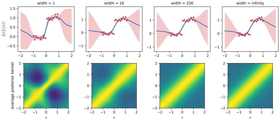
fig_sup18_4. Reproduces Murphy (2023), Supplement Figure 18.4. Download: PDF · SVGS18.1.0.5 Connection with Bayesian neural networks
supplement pp. 187–188, (S18.12) A Bayesian neural network (BNN) puts priors on the weights of a network (Chapter 17 of the book); one can show that BNNs are a degenerate form of DGP (Ober and Aitchison, 2021). For a 2-layer MLP \(f_2(f_1(\bm x))\) with \(f_1^{(i)}(\bm x)=(\bm w_1^{(i)})^\T\bm x+\beta b_1\) and \(f_2(\bm z)=\frac1{\sqrt{H_1}}\bm w_2^\T\varphi(\bm z)+\beta b_2\) with Gaussian weights, the first layer is Bayesian linear regression, so by Section 18.3.3 a GP with the linear kernel \(K_1(\bm x,\bm x')=\bm x^\T\bm x'\) (plus a constant); the second is linear regression on the features \(\varphi(\bm z)\), a GP with \(K_2(\bm z,\bm z')=\varphi(\bm z)^\T\varphi(\bm z')\). Each layer is therefore a GP with a finite number of non-zero eigenvalues ("degenerate"), so the network is a degenerate DGP. By the limit result above, infinitely wide DNNs reduce to a single-layer GP, as in Section 18.7.1. Finite networks should be wide enough that each layer is close to a GP, but not so wide that the layer kernels stop adapting to the data (no feature learning); see Aitchison (2020), Pleiss and Cunningham (2021) and Zavatone-Veth et al. (2021).
S18.2 GPs and SSMs
supplement p. 188, (S18.13)–(S18.22) The matrices for the Matérn \(\frac32\) and \(\frac52\) kernels, the transition matrices \(\bm A_{k}=\exp(\bm F\Delta_k)\), the noise covariance \(\bm Q_k\) and the spectral-density constant \(q\) are written out in Section 18.5.6 above, and their derivation (spectral density, Lyapunov equation, equality of the Kalman smoother with GP regression) is Gap 18.21. (The supplement writes the \(\frac52\) kernel as \(1+\sqrt5r/\ell+5\tau^2/(3\ell^2)\), mixing \(r\) and \(\tau\); both mean the lag.)
Demonstrations for this chapter
Each demonstration runs in the browser, with seeded random numbers so that a class sees the same pictures, and links back to these notes. The ▶ Demo boxes above open them already set to the case under discussion. Where a demonstration uses the book's data or a figure's data set, the numbers it shows are those of the Python code.
| Demonstration | What you can see | Sections and results |
|---|---|---|
| Building kernels: sums, products and random features | Eight elementary kernels, their sum or product, the kernel against a fixed second input and four prior draws; a mode with random Fourier features of the SE kernel and their error. Presets: 1 Matérn 1/2; 2 SE × periodic; 3 linear × periodic; 4 SE + periodic; 5 random features, D = 10. | 18.2.1, 18.2.4 (gap 18.4), 18.2.6 (gap 18.6) |
| Sparse GPs: inducing points and the variance they lose | Exact GP against SOR, DTC, FITC and VFE on 90 points with a gap; number and placement of the inducing points, the training objective against the exact log marginal likelihood, and the predictive standard deviation. Presets: 1 SOR, M = 6; 2 VFE, M = 6; 3 FITC, M = 3; 4 greedy placement; 5 VFE with all data. | 18.5.3 (gap 18.16), 18.5.4 (gap 18.17) |
| Forecasting CO2 with a sum of kernels | The four-part kernel of Section 18.8.1 on the Mauna Loa record: switch parts off, move the cut-off year, change the trend length scale, the seasonal decay and the noise; the forecast, its band, the log marginal likelihood, the held-out RMSE and the contribution of each part. Presets: 1 full model; 2 trend only; 3 no periodic part; 4 cut-off 1975; 5 short trend length scale. | 18.8.1, 18.6.1 (gap 18.22) |
The Python code that produces every figure of this page is code/ch18_gaussian_processes.py (see the code index).
Practice problems
The book has no exercises for this chapter. These three short problems are my own.
Practice problem 18.1 (one observation). A GP with SE kernel (\(\ell=1\), variance 1) and zero mean observes a single data point \(y=1.5\) at \(x=0\) with noise variance \(\sigma^2=0.25\). Give the posterior mean and variance of \(f(1)\).
Solution
With \(N=1\): \(K_\sigma=1+0.25=1.25\), \(k_*=K(1,0)=e^{-1/2}=0.6065\), \(k_{**}=1\). By (18.52)–(18.53), \(\mu_*=k_*K_\sigma^{-1}y=0.6065\cdot1.5/1.25=0.7278\) and \(\sigma_*^2=1-k_*^2/1.25=1-0.3679/1.25=0.7057\). The mean is the data value shrunk by the noise (\(1/1.25\)) and by the correlation (0.607); the variance has dropped from 1 to 0.706. A numerical computation with the Cholesky code agrees.
Practice problem 18.2 (how many random features?). Random Fourier features approximate the SE kernel. At a separation where the exact kernel value is \(K=0.5\), what is the standard deviation of the estimate with \(D=100\) frequencies, and how large must \(D\) be to bring it below 0.01?
Solution
By Gap 18.6, \(\var[\hat K]=(1-K^2)^2/(2D)\), so the standard deviation is \((1-K^2)/\sqrt{2D}=0.75/\sqrt{200}=0.0530\) for \(D=100\). It is below 0.01 when \(\sqrt{2D}>75\), i.e. \(2D>5625\), so \(D\ge2813\). Because the standard deviation falls like \(D^{-1/2}\), reducing it by a factor 5.3 needs 28 times more features, which is why random features need many frequencies for high accuracy.
Practice problem 18.3 (SOR against DTC far from the data). Take the SE kernel (variance 1, \(\ell=1\)), noise variance \(\sigma^2\), a single inducing point \(z=0\) and \(n\) training inputs all located at \(x=0\). Give the SOR and DTC predictive variances of \(f(x_*)\) and their limits as \(|x_*|\to\infty\).
Solution
Here \(K_{ZZ}=1\), \(\bm K_{Z,X}=\bm 1^\T\) (all ones, length \(n\)), \(K(x_*,Z)=k_*=e^{-x_*^2/2}\). So \(\Sigma=(\sigma^{-2}\bm K_{Z,X}\bm K_{X,Z}+K_{ZZ})^{-1}=(1+n/\sigma^2)^{-1}\). By (18.123) the SOR variance is \(k_*\Sigma k_*=k_*^2/(1+n/\sigma^2)\). By (18.127) the DTC variance adds \(k_{**}-Q_{**}=1-k_*^2\), giving \(1-k_*^2+k_*^2/(1+n/\sigma^2)\). As \(|x_*|\to\infty\), \(k_*\to0\): SOR variance \(\to0\) (a degenerate GP, certain about a function it cannot see) while DTC variance \(\to1\), the prior variance, as it should be. Checked numerically for \(n=10\), \(\sigma^2=0.5\), \(x_*=3\).
Notes on the book
Errors and slips found, with where the evidence is
- (18.21), rational quadratic as a mixture: the mixing law must be a gamma with shape \(\alpha\) and rate \(\alpha\ell^2\) (so that its mean is \(1/\ell^2\)); the text's "\(\mathrm{Ga}(\alpha,\ell^2)\)" lacks the factor \(\alpha\) (Gap 18.1, confirmed by quadrature).
- Section 18.2.1.6, SE spectral density: with \(K(\delta)=\int p(\omega)e^{j\omega\delta}\d\omega\) as printed, the density is \(\frac{\ell}{\sqrt{2\pi}}e^{-\ell^2\omega^2/2}\); the printed \(\sqrt{2\pi}\ell^2e^{-2\pi^2\omega^2\ell^2}\) mixes the conventions (it is the ordinary-frequency density but with \(\ell^2\) in place of \(\ell\), so it integrates to \(\ell\), not 1) (Gap 18.2).
- (18.42): \(\bm\phi(\bm x)^\T\bm\phi(\bm x)\) should be \(\bm\phi(\bm x)^\T\bm\phi(\bm x')\) (Gap 18.6).
- (18.62): \(\sigma_y\bm I\) should be \(\sigma_y^2\bm I\) (Gap 18.8).
- (18.107) and (18.108): the second term of the Woodbury inverse has a minus sign, not a plus; the determinant needs the factor \(\sigma^{2(N-M)}\) (Gap 18.15, confirmed numerically; the printed forms differ from the true values by an order-one amount).
- Table 18.4: with \(\bm u\sim\N(\bm0,\tilde{\bm\Sigma})\) the Heaviside entry is \((\pi-\theta)/(2\pi)\) and the ReLU entry is half of the printed expression; the printed table is correct only up to positive constants (\(2\pi\) and \(2\)), which the output variance absorbs; the erf row is exact (Gap 18.24, Monte Carlo).
- Figure 18.16 caption: the two marked points are local maxima of the log marginal likelihood (minima of its negative), not local minima; and the weak statement "the more complex model has a marginal likelihood about 60% higher" concerns the likelihood, not the log likelihood.
- (minor) (18.11) a product of \(D\) SE factors each with amplitude \(\sigma^2/D\) has amplitude \((\sigma^2/D)^D\), not \(\sigma^2\); one factor must carry \(\sigma^2\) (Section 18.2.1.2). (18.99) the white-noise kernel uses a Kronecker, not Dirac, delta. (18.163) \(\bm y^\T\) missing in the quadratic form. (18.26) \(x_2x_2\) for \(x_2x_2'\). Supplement (S18.15) mixes \(r\) and \(\tau\) for the lag. Section 18.5.6 the amplitude of the exponential kernel is \(q/(2\lambda)\) in terms of the SDE's spectral density \(q\), and need not be \(\sqrt{2\lambda}\).
References
- Murphy, K. P. (2023). Probabilistic Machine Learning: Advanced Topics. MIT Press, Cambridge, MA. Chapter 18, pp. 681–733, and Supplementary Chapter 18. probml.github.io/pml-book/book2.html.
- Arora, S., Du, S. S., Hu, W., Li, Z., Salakhutdinov, R. and Wang, R. (2019). On exact computation with an infinitely wide neural net. Advances in Neural Information Processing Systems, 32.
- Bach, F. (2009). High-dimensional non-linear variable selection through hierarchical kernel learning. arXiv:0909.0844.
- Cho, Y. and Saul, L. K. (2009). Kernel methods for deep learning. Advances in Neural Information Processing Systems, 22.
- Chizat, L., Oyallon, E. and Bach, F. (2019). On lazy training in differentiable programming. Advances in Neural Information Processing Systems, 32.
- Damianou, A. and Lawrence, N. D. (2013). Deep Gaussian processes. Artificial Intelligence and Statistics.
- Duvenaud, D., Lloyd, J. R., Grosse, R., Tenenbaum, J. B. and Ghahramani, Z. (2013). Structure discovery in nonparametric regression through compositional kernel search. International Conference on Machine Learning.
- Gibbs, M. N. (1997). Bayesian Gaussian processes for regression and classification. PhD thesis, University of Cambridge.
- Härkönen, J. and Särkkä, S. (2010). Spatio-temporal Gaussian process regression as a state space model (see also Hartikainen and Särkkä, 2010, Kalman filtering and smoothing solutions to temporal Gaussian process regression models, IEEE MLSP).
- Hensman, J., Fusi, N. and Lawrence, N. D. (2013). Gaussian processes for big data. Uncertainty in Artificial Intelligence.
- Jacot, A., Gabriel, F. and Hongler, C. (2018). Neural tangent kernel: convergence and generalization in neural networks. Advances in Neural Information Processing Systems, 31.
- Lee, J., Bahri, Y., Novak, R., Schoenholz, S. S., Pennington, J. and Sohl-Dickstein, J. (2018). Deep neural networks as Gaussian processes. International Conference on Learning Representations.
- Neal, R. M. (1996). Bayesian Learning for Neural Networks. Springer.
- Pleiss, G. and Cunningham, J. P. (2021). The limitations of large width in neural networks: a deep Gaussian process perspective. Advances in Neural Information Processing Systems, 34.
- Quiñonero-Candela, J. and Rasmussen, C. E. (2005). A unifying view of sparse approximate Gaussian process regression. Journal of Machine Learning Research, 6, 1939–1959.
- Rahimi, A. and Recht, B. (2008). Random features for large-scale kernel machines. Advances in Neural Information Processing Systems, 20.
- Rasmussen, C. E. and Williams, C. K. I. (2006). Gaussian Processes for Machine Learning. MIT Press.
- Rue, H., Martino, S. and Chopin, N. (2009). Approximate Bayesian inference for latent Gaussian models by using integrated nested Laplace approximations. Journal of the Royal Statistical Society B, 71(2), 319–392.
- Salimbeni, H. and Deisenroth, M. (2017). Doubly stochastic variational inference for deep Gaussian processes. Advances in Neural Information Processing Systems, 30.
- Särkkä, S. and Solin, A. (2019). Applied Stochastic Differential Equations. Cambridge University Press.
- Snelson, E. and Ghahramani, Z. (2006). Sparse Gaussian processes using pseudo-inputs. Advances in Neural Information Processing Systems, 18.
- Titsias, M. (2009). Variational learning of inducing variables in sparse Gaussian processes. Artificial Intelligence and Statistics.
- Wang, K. A., Pleiss, G., Gardner, J. R., Tyree, S., Weinberger, K. Q. and Wilson, A. G. (2019). Exact Gaussian processes on a million data points. Advances in Neural Information Processing Systems, 32.
- Williams, C. K. I. (1998). Computation with infinite neural networks. Neural Computation, 10(5), 1203–1216.
- Wilson, A. G. and Adams, R. P. (2013). Gaussian process kernels for pattern discovery and extrapolation. International Conference on Machine Learning.
- Wilson, A. G. and Nickisch, H. (2015). Kernel interpolation for scalable structured Gaussian processes (KISS-GP). International Conference on Machine Learning.
- Wilson, A. G., Hu, Z., Salakhutdinov, R. and Xing, E. P. (2016). Deep kernel learning. Artificial Intelligence and Statistics.
- Zhu, H., Williams, C. K. I., Rohwer, R. and Morciniec, M. (1998). Gaussian regression and optimal finite dimensional linear models. In Neural Networks and Machine Learning, Springer.
The numerical statements in the text (closure of the kernels under sums, products, exponentials and the Gibbs construction; the rational quadratic as a gamma mixture; the spectral densities of the SE, Matérn and spectral mixture kernels; random Fourier features and their variance; GP posterior formulas against brute-force conditioning; weight space against function space; the semi-parametric GP and its limit; the marginal-likelihood gradient, leave-one-out formulas and length-scale limits; kernel ridge regression and the representer theorem; the scikit-learn marginal likelihood for the periodic GP and the Laplace GP classifier; the probit approximation; the Woodbury and determinant corrections; the Nyström, SOR, DTC, FITC and variational formulas and bound properties; conjugate-gradient and Lanczos estimates; the Toeplitz and SKI statements; the Matérn state space models and Kalman smoother; the NN-GP kernels; the neural tangent kernel; the deep-GP limit kernel; and the values the three demonstrations show) were confirmed numerically.