Reinforcement learning
Chapter 34 solved Markov decision processes whose model is known. Here the model is unknown and the agent has to learn from the trajectories it generates. The chapter surveys the three routes (learn a value function, search the policy directly, or learn a model and plan with it), the exploration problem that sits across all three, and the off-policy and probabilistic ideas that connect them to the rest of the book. These notes supply the arguments that the survey leaves out: why temporal-difference methods and Q-learning converge, why the maximum over noisy estimates is biased, the policy gradient theorem and the variance of its estimators, the performance-difference lemma behind conservative and trust-region updates, the Riccati recursion for model predictive control, the exponential variance of importance sampling and the stationary-ratio fix, why Baird's counterexample diverges, and how maximum-entropy RL falls out of a KL divergence.
Ch. 1 Introduction Ch. 2 Probability Ch. 3 Statistics Ch. 4 Graphical models Ch. 5 Information theory Ch. 6 Optimisation Ch. 7 Inference algorithms Ch. 8 Gaussian filtering Ch. 9 Message passing Ch. 10 Variational inference Ch. 11 Monte Carlo Ch. 12 MCMC Ch. 13 Sequential Monte Carlo Ch. 14 Predictive models Ch. 15 GLMs Ch. 16 Deep networks Ch. 17 Bayesian neural networks Ch. 18 Gaussian processes Ch. 19 Beyond iid Ch. 20 Generative models Ch. 21 VAEs Ch. 22 Autoregressive models Ch. 23 Normalizing flows Ch. 24 Energy-based models Ch. 25 Diffusion models Ch. 26 GANs Ch. 27 Discovery methods Ch. 28 Latent factor models Ch. 29 State-space models Ch. 30 Graph learning Ch. 31 Nonparametric Bayes Ch. 32 Representation learning Ch. 33 Interpretability Ch. 34 Decision making Ch. 35 Reinforcement learning Ch. 36 Causality
How to read these notes
They follow the book. Sections carry the book's numbers. I keep the book's equation numbers where I restate an equation, e.g. (35.12), (35.21), (35.47). The chapter is a survey of a very large literature and states most results without proof, so most of the work here is in the gap boxes.
Filling the gaps. Where the book quotes a result I prove it (convergence of TD and Q-learning, the policy gradient theorem, the performance-difference lemma and the conservative and trust-region bounds, the deterministic policy gradient, the value of model predictive control, the Riccati recursion, importance sampling and the doubly robust estimator, the saddle point of the stationary-ratio problem, the divergence of Baird's counterexample, the maximum-entropy objective, the f-divergence bound), or I say precisely what is left to the references. Each box starts hidden: click its bar. The text and the formulas I changed or corrected are listed under Notes on the book.
Figures. Figures 35.4, 35.5 and 35.10(b) are reproduced with my own code (the exploration sequence of 35.4 is my own draw, and 35.5 uses 4000 runs and eight actions in state B). Figures 35.1 to 35.3, 35.6 to 35.9, 35.10(a) and 35.11 are diagrams, photographs or architecture sketches with nothing to compute. Figures 35.12 to 35.17 are my own additions: TD(\(\lambda\)) on a random walk, REINFORCE with baselines, the curse of horizon, the conservative and trust-region bounds, model predictive control with a terminal value, and maximum-entropy RL. Table 35.2 is recomputed.
The supplement. The supplement chapter S35 consists of a title page only in this draft; Supplement S35 says so.
Main reference
K. P. Murphy, Probabilistic Machine Learning: Advanced Topics, MIT Press (2023; December 2025 draft), Chapter 35 (co-authored with Lihong Li), pages 1145–1183 (book page: probml.github.io/pml-book/book2.html). The explanations, derivations, figures and code are my own.
Companion courses
- This course, Chapter 34 (decision making under uncertainty) is the prerequisite. It defines the MDP and the return (34.5), proves the Bellman equations and that the Bellman operators are contractions (gap 34.21), proves value iteration, policy iteration (the policy improvement theorem) and the two linear programs (34.24, 34.25, 34.26), and treats bandits with UCB and Thompson sampling and the Lai-Robbins bound (34.4). I use those results freely and do not repeat them.
- This course: 6.3.4 the score function estimator (the log-derivative trick behind REINFORCE), 6.4 natural gradient descent (Section 35.3.4), 6.7.5 the cross-entropy method and evolution strategies (35.3.6, 35.4.1.3), 11.5 importance sampling (35.5.1), Chapter 18 (Gaussian processes, 35.4.3), 17.3.9 deep ensembles and 17.3.1 MC dropout (35.4.4), 29.13.2 recurrent state-space models (35.4.5), 19.5.2 weighted ERM under covariate shift (the off-policy correction of 35.5), 2.7.1 f-divergences and 26.2.3 bounds on f-divergences (35.6.3.3).
- Probabilistic Machine Learning: An Introduction: Chapter 5 (decision theory) for the maximum expected utility principle that this chapter starts from.
What this chapter adds: the stochastic-approximation proof that behind tabular TD and Q-learning, the exact Bayes-adaptive solution of a small unknown MDP next to Thompson sampling, a complete proof of the policy gradient theorem and of the conservative and trust-region bounds (with the constant I can prove), the optimal baseline, the finite-horizon Riccati recursion and its certainty equivalence, the exact Gaussian moments of a GP prediction, the exponential variance of trajectory importance weights, the saddle point of the stationary-ratio problem, a spectral explanation of Baird's counterexample and of the double-sampling problem, and the exact relation between exact control-as-inference and soft Bellman backups.
The chapter at a glance
- 35.1 The TD error is the Bellman error and TD is not SGD (gap 35.1); epsilon-greedy and Boltzmann exploration (35.2); optimism from count bonuses (35.3); the Bayes-adaptive MDP (35.4).
- 35.2 Monte Carlo control and epsilon-soft policies (gap 35.5); the convergence of TD, Q-learning and SARSA (35.6); batch TD against batch Monte Carlo (35.7); the lambda-return and eligibility traces (35.8); the maximisation bias (35.9); fitted Q-iteration and DQN (35.10).
- 35.3 The policy gradient theorem (gap 35.11); baselines (35.12); advantage estimation (35.13); the performance-difference lemma and the CPI and TRPO bounds (35.14); natural gradient and PPO (35.15); deterministic policy gradients (35.16).
- 35.4 Model predictive control with a terminal value, and A* (gap 35.17); LQR and LQG (35.18); a GP at a Gaussian input (35.19); common random numbers (35.20).
- 35.5 Importance sampling and per-decision importance sampling (gap 35.21); the doubly robust estimator (35.22); the curse of horizon and the stationary ratio (35.23); linear TD and the deadly triad (35.24); double sampling, PCL and SBEED (35.25).
- 35.6 Maximum-entropy RL and exact control as inference (gap 35.26); behaviour cloning (35.27); maximum-entropy inverse RL (35.28); the f-divergence bound for imitation (35.29).
Notation. Time starts at 0 in this chapter (the book's remark: it starts at 1 for bandits). \(s_t,a_t,r_t\) are the state, action and reward, \(\gamma\) the discount, \(G_t=\sum_{k\ge0}\gamma^kr_{t+k}\) the return, \(\pi\) a policy, \(V_\pi,Q_\pi\) its value functions, \(A_\pi=Q_\pi-V_\pi\) the advantage, \(T_\pi,T_*\) the Bellman operators of Chapter 34, \(p_t\) the state distribution at time \(t\) and \(p^\infty_\pi=(1-\gamma)\sum_t\gamma^tp_t\) the normalised discounted state distribution, \(J(\pi)=\E_{p_0,\pi}[G_0]\) (35.15). Vectors and matrices: \(\Phi\) a feature matrix, \(D=\diag(d)\) a state distribution, \(P_\pi\) the state transition matrix of \(\pi\).
35.1 Introduction
p. 1145 In reinforcement learning (RL) an agent interacts with an initially unknown environment and produces trajectories \(\tau=(s_0,a_0,r_0,s_1,\dots,s_T)\). It chooses its actions with a policy and tries to maximise the expected discounted return \(G_0=\sum_{t=0}^{T-1}\gamma^tr_t\) (the maximum expected utility principle of Chapter 34; risk-sensitive criteria such as the conditional value at risk, the mean of the worst 5% of outcomes, are alternatives). The generative model of a trajectory factorises into one-step models (a Markov decision process); with known parameters finding the best policy is planning (Section 34.6), otherwise it is learning. In model-free RL the policy or a value function is learned directly from trajectories; in model-based RL one learns \(p(s'\given s,a)\) and \(R(s,a)\) first and plans with them. The chapter follows the notation of Sutton and Barto (2018), which is also the best general textbook reference.
35.1.1 Overview of methods
pp. 1145–1146, Figure 35.1, Table 35.1 Methods are sorted by what they represent (a value function, a policy, a model) and by how the actions that feed learning are chosen: on-policy methods learn from actions drawn from the policy they are improving (SARSA, REINFORCE, A2C, TRPO/PPO), off-policy methods can learn from any behaviour (Q-learning, DDPG, soft actor-critic, model-based RL). The table in the book lists the functions each method learns: SARSA and Q-learning learn \(Q(s,a)\); REINFORCE learns \(\pi\); A2C learns \(\pi\) and \(V\); TRPO/PPO learn \(\pi\) and \(A\); DDPG learns a deterministic \(\mu\) and \(Q\); soft actor-critic learns \(\pi\) and \(Q\); model-based RL learns \(p(s'\given s,a)\). Figure 35.1 is a map and nothing in it is computed.
35.1.2 Value-based methods
p. 1147 A value-based method learns the optimal action-value function \(Q_*\) with a function approximator \(Q_{\bm w}\) and acts greedily (34.84). Given a transition \((s,a,r,s')\) the temporal-difference (TD) error is \[ \delta=r+\gamma\max_{a'}Q_{\bm w}(s',a')-Q_{\bm w}(s,a). \] Its expectation is the Bellman error at \((s,a)\), so it vanishes on average exactly when \(Q_{\bm w}=Q_*\), and otherwise it tells the agent how to move \(Q_{\bm w}(s,a)\) toward the bootstrapped target \(r+\gamma\max_{a'}Q_{\bm w}(s',a')\), which is computed from the estimate itself. (This is unrelated to the statistical bootstrap.) Gap 35.1 proves the first claims and shows why the resulting update is not stochastic gradient descent on any objective.
Filling the gap 35.1: the TD error is the Bellman error; TD is not SGD pp. 1147, 1151, (35.6), (35.7)
Derivation
The expected TD error. Conditionally on \((s_t,a_t)=(s,a)\), \(r\) has mean \(R(s,a)\) and \(s'\sim p(\cdot\given s,a)\), so \[ \E[\delta\given s,a]=R(s,a)+\gamma\sum_{s'}p(s'\given s,a)\max_{a'}Q_{\bm w}(s',a')-Q_{\bm w}(s,a)=(T_*Q_{\bm w}-Q_{\bm w})(s,a), \] the Bellman error (\(T_*\) is the optimality operator of gap 34.21). Since \(T_*\) is a \(\gamma\)-contraction in the sup norm with the unique fixed point \(Q_*\), the Bellman error is zero at every \((s,a)\) if and only if \(Q_{\bm w}=Q_*\), and \(\|Q-Q_*\|_\infty\le\|T_*Q-Q\|_\infty/(1-\gamma)\). I checked the first identity by averaging 400,000 sampled TD errors (agreement within sampling error) and that the Bellman error of \(Q_*\) is zero to \(10^{-10}\).
Why (35.7) is not stochastic gradient descent. Consider the squared loss of one transition, \(\tfrac12(r+\gamma V_{\bm w}(s')-V_{\bm w}(s))^2\). Its true gradient is \(\delta\,(\gamma\nabla V_{\bm w}(s')-\nabla V_{\bm w}(s))\). The TD update \(\delta\nabla V_{\bm w}(s)\) (35.7) treats the target as a constant and drops the term \(\gamma\nabla V_{\bm w}(s')\); that is why it is called a semi-gradient method. It is not the gradient of any other objective either: for a linear approximation \(V_{\bm w}=\Phi\bm w\), with states drawn from a distribution \(d\) (\(D=\diag(d)\)) and \(P\) the transition matrix of the policy, the expected update is the vector field \[ F(\bm w)=\bm b-A\bm w,\qquad A=\Phi^\T D(I-\gamma P)\Phi,\quad \bm b=\Phi^\T D\bm r. \] A smooth vector field is a gradient field only if its Jacobian \(-A\) is symmetric. \(A\) is not symmetric in general (for a random six-state chain with three random features, \(\|A-A^\T\|_F=0.63\) against \(\|A\|_F=1.58\)), so no loss exists whose negative gradient is the expected TD update. Convergence therefore needs a separate argument, which gap 35.6 gives for the tabular case and gap 35.24 for the linear case.
35.1.3 Policy search methods
p. 1147 Policy search maximises \(J(\pi_{\bm\theta})\) over the policy parameters by stochastic gradient ascent (policy gradient, Section 35.3.1). \(J\) is an expectation under a distribution that depends on \(\bm\theta\), so the gradient cannot be moved inside the expectation; the score function estimator (Section 6.3.4) replaces it. Policy gradient methods converge to a local optimum for many policy classes, handle continuous actions without maximising \(Q\) over actions, but have high variance; a learned baseline \(V_{\bm w}(s)\) or advantage \(A_{\bm w}(s,a)\) reduces the variance and gives actor-critic methods (the actor is \(\pi_{\bm\theta}\), the critic is \(V_{\bm w}\) or \(A_{\bm w}\)).
35.1.4 Model-based RL
pp. 1147–1148 Value-based and policy-search methods can be very sample-inefficient. Model-based RL first learns \(p(s'\given s,a)\) and \(R(s,a)\) by supervised learning from \((s,a,r,s')\) tuples, then runs a model-free algorithm on synthetic experience or a planning algorithm on the model, usually interleaving the two so that the partly learned policy decides what data to collect (Section 35.4).
35.1.5 Exploration-exploitation tradeoff
p. 1148 With unknown transition and reward models the agent must choose between actions it knows to be good and actions whose value is uncertain but may lead to better regions of the state-action space. The simpler contextual-bandit version is Section 34.4.3. The book describes several techniques.
35.1.5.1 ε-greedy
p. 1148 The policy \(\pi_\epsilon\) takes the greedy action \(a_t=\argmax_a\hat R_t(s_t,a)\) with probability \(1-\epsilon\) and a uniformly random action otherwise. Every action keeps probability at least \(\epsilon/|\mathcal A|\) forever, which is why the rule is suboptimal: the exploration never stops.
35.1.5.2 Boltzmann exploration
p. 1148 The Boltzmann (softmax) policy \[ \pi_\tau(a\given s)=\frac{\exp(\hat R_t(s_t,a)/\tau)}{\sum_{a'}\exp(\hat R_t(s_t,a')/\tau)} \tag{35.1} \] with temperature \(\tau>0\) tends to the greedy policy as \(\tau\to0\) and to the uniform policy as \(\tau\to\infty\), and its probabilities depend smoothly on the reward estimates, unlike \(\epsilon\)-greedy (Table 35.2, recomputed below). Gap 35.2 proves these statements.
| \(\hat R(s,a_1)\) | \(\hat R(s,a_2)\) | \(\pi_\epsilon(a_1)\) | \(\pi_\epsilon(a_2)\) | \(\pi_\tau(a_1)\) | \(\pi_\tau(a_2)\) |
|---|---|---|---|---|---|
| 1.00 | 9.00 | 0.05 | 0.95 | 0.00 | 1.00 |
| 4.00 | 6.00 | 0.05 | 0.95 | 0.12 | 0.88 |
| 4.90 | 5.10 | 0.05 | 0.95 | 0.45 | 0.55 |
| 5.05 | 4.95 | 0.95 | 0.05 | 0.525 | 0.475 |
| 7.00 | 3.00 | 0.95 | 0.05 | 0.98 | 0.02 |
| 8.00 | 2.00 | 0.95 | 0.05 | 1.00 | 0.00 |
Filling the gap 35.2: ε-greedy regret, the limits and entropy of the Boltzmann policy, and Table 35.2 pp. 1148–1149, (35.1), Table 35.2
Derivation
ε-greedy is not consistent. Suppose the greedy action is already the best one and has gap \(\Delta_a\) to action \(a\) (take a bandit, or one state of an MDP in which the reward estimates are right). The per-step expected regret of \(\pi_\epsilon\) is \(\sum_a\pi_\epsilon(a)\Delta_a=\tfrac{\epsilon}{|\mathcal A|}\sum_a\Delta_a>0\), constant in time, so the cumulative regret is linear in \(T\). The Lai-Robbins bound of gap 34.19 is logarithmic, so a fixed \(\epsilon\) is not asymptotically efficient. (Decaying \(\epsilon_t\propto1/t\) removes the linear term but needs the size of the smallest gap to be tuned, Auer et al. 2002.) The identity was checked numerically.
The Boltzmann policy. Write \(\beta=1/\tau\), \(Z(\beta)=\sum_a e^{\beta\hat R_a}\) and \(\pi_\beta(a)=e^{\beta\hat R_a}/Z\). As \(\beta\to\infty\) the ratio \(\pi_\beta(a)/\pi_\beta(a^*)=e^{-\beta(\hat R_{a^*}-\hat R_a)}\to0\) for every non-maximal \(a\), so \(\pi_\tau\) tends to the greedy policy (ties share the mass); as \(\beta\to0\) all exponentials tend to 1, so \(\pi_\tau\) tends to the uniform policy. Its entropy is \(H=\log Z-\beta\E_\pi[\hat R]\), and \(\frac{d\log Z}{d\beta}=\E_\pi[\hat R]\), \(\frac{d}{d\beta}\E_\pi[\hat R]=\var_\pi(\hat R)\), so \[ \frac{dH}{d\beta}=\E_\pi[\hat R]-\E_\pi[\hat R]-\beta\var_\pi(\hat R)=-\beta\var_\pi(\hat R)\le0, \qquad\text{hence}\qquad \frac{dH}{d\tau}=\frac{\var_\pi(\hat R)}{\tau^3}\ge0 : \] the entropy increases with the temperature, from 0 (greedy) to \(\log|\mathcal A|\) (uniform). The sensitivity is also explicit: \(\partial\pi_\tau(a)/\partial\hat R_a=\pi_\tau(a)(1-\pi_\tau(a))/\tau\), a smooth function, whereas \(\pi_\epsilon\) jumps from \(\epsilon/|\mathcal A|\) to \(1-\epsilon+\epsilon/|\mathcal A|\) when the ranking changes. For two actions \(\pi_\tau(a_1)=\sigma((\hat R_1-\hat R_2)/\tau)\), which gives the table: \(\sigma(-8)=0.0003\), \(\sigma(-2)=0.119\), \(\sigma(-0.2)=0.450\), \(\sigma(0.1)=0.525\), \(\sigma(4)=0.982\), \(\sigma(6)=0.9975\).
A slip in the table. In the fourth row the book prints 0.53 and 0.48 for the Boltzmann pair; the two probabilities must sum to one, and \(\sigma(0.1)=0.52498\), so the correct two-decimal entries are 0.52 and 0.48 (three decimals: 0.525 and 0.475). Every other entry of the table reproduces.
35.1.5.3 Upper confidence bounds and Thompson sampling
pp. 1148–1149 UCB (34.4.5) and Thompson sampling (34.4.6) extend to MDPs, but now the uncertainty is also in the transitions. Count-based exploration adds a bonus to the reward of every observed transition, \[ \tilde r=r+\frac{\alpha}{\sqrt{N_{s,a}}}, \tag{35.2} \] where \(N_{s,a}\) counts visits of \((s,a)\) and \(\alpha\ge0\) sets the amount of exploration; this is the MBIE-EB method (Strehl and Littman 2008), extended to continuous states by hashing (Bellemare et al. 2016). MBIE, UCRL2 and UCBVI keep explicit confidence sets over the transition probabilities. Thompson sampling keeps a posterior over the reward and transition parameters; for a finite MDP a Dirichlet prior on each categorical transition row is conjugate, so the posterior is cheap to update and sample (Russo et al. 2018). Both families have provable regret or sample-complexity bounds for finite MDPs. Gap 35.3 shows where the \(1/\sqrt N\) bonus comes from and why it produces optimism.
Filling the gap 35.3: a count-based bonus makes the learned Q-function optimistic pp. 1148–1149, (35.2)
Derivation
Setting. Rewards lie in \([0,1]\), so \(0\le V_*\le V_{\max}=1/(1-\gamma)\). From \(N\) samples at each pair \((s,a)\) build the empirical reward \(\hat R(s,a)\) and transition \(\hat P(\cdot\given s,a)\). Fix \(\delta\in(0,1)\) and let \(w=\sqrt{\ln(4|\mathcal S||\mathcal A|/\delta)/(2N)}\).
The good event. The variable \(\hat R(s,a)\) is an average of \(N\) independent variables in \([0,1]\), and \((\hat P-P)V_*=\frac1N\sum_i V_*(s'_i)-\E V_*(s')\) is an average of \(N\) independent variables in \([0,V_{\max}]\) (\(V_*\) is fixed, not data dependent). Hoeffding's inequality and a union bound over the \(2|\mathcal S||\mathcal A|\) quantities give, with probability at least \(1-\delta\), for all \((s,a)\): \(|\hat R-R|\le w\) and \(|(\hat P-P)V_*|\le V_{\max}w\). Therefore \[ \bigl|\hat R+\gamma\hat PV_*-R-\gamma PV_*\bigr|\le w+\gamma V_{\max}w=V_{\max}w=:b, \] a bonus of the form \(\alpha/\sqrt N\) with \(\alpha=\sqrt{\ln(4|\mathcal S||\mathcal A|/\delta)/2}/(1-\gamma)\).
Optimism. Let \(\tilde T\) be the Bellman optimality operator of the empirical model with the bonus added to the reward, \((\tilde TQ)(s,a)=\hat R+b+\gamma\hat P\max_{a'}Q\), and \(\tilde Q\) its fixed point. On the good event \(\tilde TQ_*\ge R+\gamma P\max Q_*=Q_*\) componentwise. \(\tilde T\) is monotone, so \(\tilde T^{k+1}Q_*\ge\tilde T^kQ_*\ge\dots\ge Q_*\), and \(\tilde T^kQ_*\to\tilde Q\) by contraction. Hence \(\tilde Q\ge Q_*\): acting greedily on \(\tilde Q\) never undervalues an action, so a rarely tried action (large bonus) looks attractive until it has been sampled enough, exactly as in UCB.
Check. On 200 random MDPs (4 states, 2 actions, \(\gamma=0.7\), \(N=300\), \(\delta=0.1\)) the event held in all 200 trials and \(\tilde Q\ge Q_*\) held in all of them (the Hoeffding widths are conservative).
35.1.5.4 Optimal solution using Bayes-adaptive MDPs
pp. 1149–1150, (35.3)–(35.5) The Bayes-optimal exploration is the optimal policy of a special POMDP, the Bayes-adaptive MDP (BAMDP). Its state is \((s_t,b_t)\), where \(b_t=p(R,T\given h_t)\) is the belief about the reward and transition models given the history \(h_t\); this extends the Gittins-index setting of Section 34.4.4 to MDPs. The augmented model is \[ T^+(s_{t+1},b_{t+1}\given s_t,b_t,a_t,r_t)=\E_{b_t}[T(s_{t+1}\given s_t,a_t)]\;\ind\bigl(b_{t+1}=p(R,T\given h_{t+1})\bigr), \tag{35.3, 35.4} \] with \(\E_{b_t}[T]\) the posterior predictive distribution over next states, and the reward \(R^+=\E_{b_{t+1}}[R(s_t,a_t,s_{t+1})]\) (35.5). For small problems the augmented MDP can be solved exactly; in general it is intractable. The book lists approximations: Bayes-optimal-like behaviour except in a provably small number of steps (Kolter and Ng 2009), Monte Carlo rollouts (Guez et al. 2013), and a meta-learning method (Zintgraf et al. 2020) that trains a policy over many related tasks with a VAE-inferred task embedding standing in for the belief. Gap 35.4 derives (35.3, 35.4) and solves a small BAMDP exactly.
Filling the gap 35.4: the Bayes-adaptive MDP, derived, and solved exactly for a small unknown MDP pp. 1149–1150, (35.3)–(35.5)
Derivation
Why \((s,b)\) is Markov. Let \(\theta=(R,T)\) be the unknown model parameters with prior \(b_0\), and let the history be \(h_t=(s_0,a_0,r_0,\dots,s_t)\). Given \(\theta\) the environment is Markov, so \(p(s_{t+1}\given h_t,a_t,\theta)=T_\theta(s_{t+1}\given s_t,a_t)\). Marginalising \(\theta\) over the posterior \(b_t=p(\theta\given h_t)\), \[ p(s_{t+1}\given h_t,a_t)=\int T_\theta(s_{t+1}\given s_t,a_t)\,b_t(\theta)\,\d\theta=\E_{b_t}[T(s_{t+1}\given s_t,a_t)], \] which is the first factor of (35.4); it depends on the history only through \((s_t,b_t)\). The next belief is a deterministic function of the old belief and the new transition, by Bayes' rule, \(b_{t+1}(\theta)\propto b_t(\theta)\,T_\theta(s_{t+1}\given s_t,a_t)\,p(r_t\given s_t,a_t,s_{t+1},\theta)\), which is the indicator factor of (35.4). Hence the process \((s_t,b_t)\) is a controlled Markov chain, and the expected return of any history-dependent policy under the Bayesian mixture, \(\int b_0(\theta)J_\theta(\pi)\,\d\theta\), is the expected return of that policy in the BAMDP. Because \((s_t,b_t)\) is a sufficient statistic of the history, an optimal policy can be taken to depend on \((s,b)\) only, and it solves the Bellman equations of the BAMDP. For a Dirichlet prior on each transition row the belief is the vector of counts, and the update adds one to the observed count.
A worked example. State 0 has two actions: safe pays 0.4 and stays; try pays 0 and moves, with an unknown probability \(\theta\sim\mathrm{Beta}(1,1)\), to an absorbing state 1 that pays 1 per step (otherwise it stays in 0). The horizon is \(H=10\) steps, undiscounted. The belief after \(k\) failed tries is \(\mathrm{Beta}(1,1+k)\), and a success ends the learning, so the BAMDP state at state 0 is \((h,a,b)\) with \(h\) steps to go. With \(\hat\theta=a/(a+b)\) the posterior mean, \[ V(h,a,b)=\max\Bigl\{0.4+V(h-1,a,b),\ \hat\theta\,(h-1)+(1-\hat\theta)\,V(h-1,a,b+1)\Bigr\}, \quad V(0,\cdot,\cdot)=0. \] Dynamic programming gives the Bayes-optimal value \(V(10,1,1)=7.2167\). It tries at \(h=10\) and at \(h=6\) even after five failures (belief \(\mathrm{Beta}(1,6)\)), and gives up earlier as the horizon shrinks: at \(h=3\) it tries from the prior but stops after two failures, and at \(h=2\) it never tries (the exploration is worth it only if enough steps remain to exploit what is learned). For comparison: always safe is 4.0; Thompson sampling (sample \(\theta\), act optimally as if it were true) averages 7.07 (40,000 runs, standard error 0.013); the perfect-information bound \(\E_\theta V_*(\theta)\), what an agent who learned \(\theta\) for free would earn, is 7.329. In this particular problem the plug-in policy that re-plans with the posterior mean at every step gives exactly the same value as the Bayes-adaptive policy (7.2167): the only action that generates information is also the only one that can pay off, so there is no pure value of information. In general (several unknown quantities and actions whose information is not worth its direct cost) re-planning with a point estimate is strictly worse than the BAMDP policy, and Thompson sampling is a randomised approximation. A simulation of the Bayes-adaptive policy agrees with the dynamic programme (7.228 ± 0.018 against 7.2167).
Cost. The belief space for an MDP with \(|\mathcal S|\) states and \(|\mathcal A|\) actions under Dirichlet priors has dimension \(|\mathcal S|^2|\mathcal A|\), so exact dynamic programming over beliefs is feasible only for tiny problems, which is why the book turns to approximations.
35.2 Value-based RL
p. 1150 The agent now has samples from \(p\) and \(p_R\) obtained by interacting with the environment, and uses them to learn optimal Q-functions from which a policy follows.
35.2.1 Monte Carlo RL
p. 1150 Since \(Q_\pi(s,a)=\E[G_t\given s_t=s,a_t=a]\) for every \(t\), one can estimate it by taking action \(a\), following \(\pi\) to the end of the episode (or until \(\gamma^t\) is negligible), and averaging the discounted returns. Combined with policy iteration (34.6.2), \(\pi_{k+1}(s)=\argmax_aQ_k(s,a)\) with \(Q_k\) estimated by Monte Carlo (MC), this is Monte Carlo control; every state visited on a trajectory can be updated. In the tabular case there is no generalisation across \((s,a)\), so every pair must keep being visited; an \(\epsilon\)-greedy policy does this. Because the method is on-policy it converges to the best \(\epsilon\)-soft policy rather than to \(\pi_*\); importance sampling can recover \(\pi_*\), but it is simpler to decrease \(\epsilon\) gradually. Gap 35.5 makes the statement about the optimal \(\epsilon\)-soft policy precise.
Filling the gap 35.5: the optimal ε-soft policy is the optimal policy of an ε-mixed MDP p. 1150
Derivation
Setting. A policy is \(\epsilon\)-soft if \(\pi(a\given s)\ge\epsilon/|\mathcal A|\) for all \((s,a)\). The \(\epsilon\)-greedy policy of a Q-function \(Q\) is \(\pi_\epsilon(a\given s)=(1-\epsilon)\ind[a=\argmax Q(s,\cdot)]+\epsilon/|\mathcal A|\).
An \(\epsilon\)-soft policy is a policy of an \(\epsilon\)-mixed MDP. Every \(\epsilon\)-soft policy can be written \(\pi=(1-\epsilon)\tilde\pi+\epsilon\,\Unif\) with \(\tilde\pi(a\given s)=(\pi(a\given s)-\epsilon/|\mathcal A|)/(1-\epsilon)\), a valid policy. Acting with \(\pi\) in the original MDP \(M=(P,R,\gamma)\) is therefore the same as acting with \(\tilde\pi\) in the MDP \(\tilde M\) whose action \(a\) executes \(a\) with probability \(1-\epsilon\) and a uniformly random action with probability \(\epsilon\): \[ \tilde P(s'\given s,a)=(1-\epsilon)P(s'\given s,a)+\frac\epsilon{|\mathcal A|}\sum_bP(s'\given s,b),\qquad \tilde R(s,a)=(1-\epsilon)R(s,a)+\frac\epsilon{|\mathcal A|}\sum_bR(s,b). \] Indeed \(\sum_a\pi(a\given s)P(s'\given s,a)=\sum_a\tilde\pi(a\given s)\tilde P(s'\given s,a)\), and likewise for \(R\), so \(V^M_\pi=V^{\tilde M}_{\tilde\pi}\). The map \(\pi\mapsto\tilde\pi\) is a bijection between \(\epsilon\)-soft policies of \(M\) and all policies of \(\tilde M\).
Consequences. (i) The optimal \(\epsilon\)-soft policy of \(M\) is the image of an optimal (deterministic, greedy) policy of \(\tilde M\), found by value iteration or policy iteration in \(\tilde M\); its value \(\tilde V_*\) satisfies \(\tilde V_*\ge V^M_\pi\) componentwise for every \(\epsilon\)-soft \(\pi\), by Chapter 34. (ii) Policy iteration that alternates evaluation of the current \(\epsilon\)-greedy policy and the \(\epsilon\)-greedy improvement \(\pi_{k+1}=\epsilon\text{-greedy}(Q_{\pi_k})\) is exactly policy iteration in \(\tilde M\) (the greedy action of \(\tilde Q\) is the greedy action of \(Q\)), so by the policy improvement theorem (gap 34.25) it improves monotonically and stops at the optimal \(\epsilon\)-soft policy. This is what Monte Carlo control with an \(\epsilon\)-greedy behaviour policy converges to. (iii) The result is not \(\pi_*\): \(\tilde V_*\le V_*\), with strict inequality when some action is bad enough that mixing in \(\epsilon\) of random behaviour costs value. Decreasing \(\epsilon\to0\) gives \(\tilde M\to M\) and \(\tilde V_*\to V_*\).
Check. For a random 4-state, 3-action MDP with \(\gamma=0.9\), \(\epsilon=0.2\): \(\epsilon\)-soft policy iteration from a random start improved monotonically and converged to \(\tilde V_*\) (difference \(8\times10^{-13}\)); a brute-force search over all 81 deterministic action choices of an \(\epsilon\)-greedy policy found the same best value (28.268177); 200 random \(\epsilon\)-soft policies were all dominated componentwise; and \(\tilde V_*\le V_*\) with strict inequality at some state.
35.2.2 Temporal difference (TD) learning
pp. 1150–1151, Figure 35.2 Monte Carlo estimates of \(Q_\pi\) have high variance (returns sum many random rewards) and need complete episodes. TD learning (Sutton 1988) instead moves the estimate toward a bootstrapped target after each transition: for \((s_t,a_t,r_t,s_{t+1})\) with \(a_t\sim\pi\), \[ V(s_t)\leftarrow V(s_t)+\eta\,[\,r_t+\gamma V(s_{t+1})-V(s_t)\,], \tag{35.6} \] and for a parametric value function \[ \bm w\leftarrow\bm w+\eta\,[\,r_t+\gamma V_{\bm w}(s_{t+1})-V_{\bm w}(s_t)\,]\,\nabla_{\bm w}V_{\bm w}(s_t). \tag{35.7} \] The bracketed term is the TD error. In the tabular case (35.6) converges to \(V_\pi\) under proper conditions; with function approximation (35.7) may diverge, and (35.7) is not stochastic gradient descent on any objective (gap 35.1). The backup diagrams in Figure 35.2 contrast the three ways of estimating a value: Monte Carlo (sample the whole trajectory), TD (sample one transition, bootstrap), dynamic programming (full expectation over actions and next states, bootstrap). Gap 35.6 proves the convergence statement; gap 35.7 shows what batch TD converges to.
Filling the gap 35.6: why tabular TD(0), Q-learning and SARSA converge (stochastic approximation with a contraction) pp. 1151, 1153, (35.6), (35.11), (35.12)
Derivation
Theorem. Let \(F:\R^d\to\R^d\) satisfy \(\|F(x)-F(y)\|_\infty\le\gamma\|x-y\|_\infty\) with \(\gamma<1\), and let \(x_*\) be its fixed point. Let \(x_{t+1}=(1-\alpha_t)x_t+\alpha_t\bigl(F(x_t)+w_t\bigr)\) with step sizes \(\alpha_t\in[0,1]\), \(\sum_t\alpha_t=\infty\), \(\sum_t\alpha_t^2<\infty\), and noise that is a martingale difference, \(\E[w_t\given\mathcal F_t]=0\), with \(\E[\|w_t\|_\infty^2\given\mathcal F_t]\le\sigma^2\) (the iterates stay bounded, see below). Then \(x_t\to x_*\) almost surely.
Proof. Split the error into a noise part and a drift part: \(x_t-x_*=u_t+v_t\), where \(u_0=0\), \(u_{t+1}=(1-\alpha_t)u_t+\alpha_tw_t\) is the pure-noise recursion, and \(v_t=x_t-x_*-u_t\). The noise part vanishes. With \(Z_t=\|u_t\|_2^2\) and \(u_t\) being \(\mathcal F_t\)-measurable, the cross term has zero mean, so \(\E[Z_{t+1}\given\mathcal F_t]\le(1-\alpha_t)^2Z_t+d\sigma^2\alpha_t^2\le Z_t-\alpha_tZ_t+d\sigma^2\alpha_t^2\) (using \((1-\alpha)^2\le1-\alpha\) for \(\alpha\in[0,1]\)). Because \(\sum\alpha_t^2<\infty\), the Robbins-Siegmund theorem (1971) says that \(Z_t\) converges almost surely and \(\sum_t\alpha_tZ_t<\infty\); since \(\sum\alpha_t=\infty\) this forces \(\liminf Z_t=0\), hence \(\lim Z_t=0\). So \(u_t\to0\) a.s.
The drift part contracts. Subtracting the two recursions gives \(v_{t+1}=(1-\alpha_t)v_t+\alpha_t\bigl(F(x_t)-x_*\bigr)\), and \(\|F(x_t)-x_*\|_\infty=\|F(x_t)-F(x_*)\|_\infty\le\gamma\|x_t-x_*\|_\infty\le\gamma(\|v_t\|_\infty+\|u_t\|_\infty)\). Fix a sample path and \(\varepsilon>0\), and let \(t_\varepsilon\) be such that \(\|u_t\|_\infty\le\varepsilon\) for \(t\ge t_\varepsilon\). With \(a_t=\|v_t\|_\infty\) and \(c=\gamma\varepsilon/(1-\gamma)\), for \(t\ge t_\varepsilon\) \[ a_{t+1}\le(1-\alpha_t)a_t+\alpha_t\gamma(a_t+\varepsilon)=\bigl(1-\alpha_t(1-\gamma)\bigr)a_t+\alpha_t\gamma\varepsilon,\qquad\text{so}\qquad a_{t+1}-c\le\bigl(1-\alpha_t(1-\gamma)\bigr)(a_t-c). \] Hence \((a_t-c)^+\le\prod_{j=t_\varepsilon}^{t-1}(1-\alpha_j(1-\gamma))\,(a_{t_\varepsilon}-c)^+\to0\), because \(\sum\alpha_j=\infty\). Thus \(\limsup\|x_t-x_*\|_\infty\le\varepsilon+c=\varepsilon/(1-\gamma)\), and letting \(\varepsilon\downarrow0\) gives \(x_t\to x_*\). \(\square\)
Applications. TD(0) for evaluation: in a tabular problem with the state updated at \(t\), \(x=V\), \(F=T_\pi\), and \(w_t\) the sampling error of \(r+\gamma V(s')\) (zero mean, bounded). Q-learning (35.12) (synchronous version, one sampled next state for every \((s,a)\) in each round): \(x=Q\), \(F=T_*\), a \(\gamma\)-contraction in the sup norm (gap 34.21), and \(w_t=r+\gamma\max_bQ(s',b)-(T_*Q)(s,a)\), a martingale difference. Boundedness: for rewards in \([0,1]\) and an initial value in \([0,V_{\max}]\), each update is a convex combination of numbers in \([0,V_{\max}]\) when \(\alpha_t\le1\), so the iterates stay in the cube and the variance bound holds. Step sizes of the form \(\alpha_t=c/(t+t_0)^{\kappa}\) with \(\kappa\in(\tfrac12,1]\) satisfy both conditions.
What the theorem does not cover. In online Q-learning only the visited pair is updated, with its own step-size sequence \(\alpha_{n(s,a)}\) and a delay between visits; the convergence proofs of Jaakkola, Jordan and Singh (1994) and Tsitsiklis (1994) extend the argument above to this asynchronous case and need every pair to be visited infinitely often (the same condition the book states). For SARSA (35.11) the target involves the next action drawn from a policy that itself changes with \(Q\); Singh et al. (2000) show that with a greedy-in-the-limit with infinite exploration (GLIE) schedule (for example \(\epsilon_t=1/t\)) it converges to \(Q_*\) and \(\pi_*\). I do not reprove these two statements.
Check. Synchronous Q-learning with \(\alpha_t=(1+0.02t)^{-3/4}\) on a random MDP (4 states, 2 actions, \(\gamma=0.7\)) reached \(\max|Q-Q_*|=0.009\) after 30,000 rounds. SARSA with \(\epsilon_k=1/(1+k/30)\) and step \(n^{-0.7}\) on the 1-D grid world ended within 0.009 of \(Q_*\).
Filling the gap 35.7: batch TD(0) converges to the certainty-equivalence value, batch Monte Carlo does not p. 1151
Derivation
Suppose a fixed set of episodes is replayed until the estimates stop changing, with the TD(0) increments summed over the whole batch before each update. At a fixed point \(\hat V\) every state satisfies \(\sum_{(s,r,s')\in\text{data},\,s\text{ fixed}}\bigl(r+\gamma\hat V(s')-\hat V(s)\bigr)=0\), i.e. \(\hat V(s)=\hat r(s)+\gamma\sum_{s'}\hat P(s'\given s)\hat V(s')\), where \(\hat r(s)\) is the average observed reward from \(s\) and \(\hat P\) the empirical transition frequencies: \(\hat V\) is the exact value function of the maximum-likelihood Markov model of the data (certainty equivalence). In contrast, the batch Monte Carlo estimate is the average observed return from each state, the least-squares fit to the returns, which ignores the Markov structure.
Example. Eight episodes: one visits \(A\) then \(B\) with both rewards 0; six visit \(B\) once and get reward 1; one visits \(B\) and gets 0. Batch TD(0) gives \(\hat V(B)=6/8=0.75\) and \(\hat V(A)=0+\hat V(B)=0.75\) (the only observed transition out of \(A\) goes to \(B\)); I ran the batch updates to convergence and obtained 0.75 for both. Batch MC gives \(\hat V(B)=0.75\) but \(\hat V(A)=0\), because the single return seen from \(A\) is 0. The TD answer uses the evidence that \(A\) leads to \(B\) and shares what is known about \(B\); the MC answer is optimal for the training returns but has no way to generalise through the model. This is one mechanism behind TD's usually better data efficiency.
35.2.3 TD learning with eligibility traces
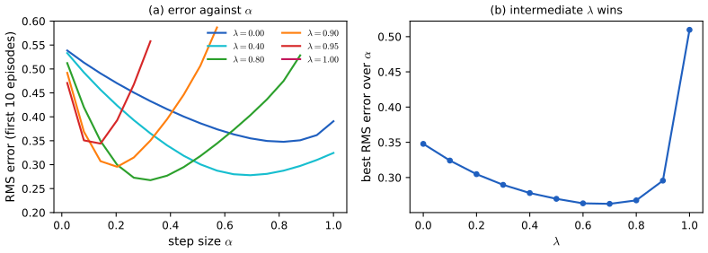
pp. 1151–1152, Figure 35.3 TD estimates the return from \(s_t\) by one-step lookahead \(G_{t:t+1}=r_t+\gamma V(s_{t+1})\); MC uses the full return \(G_{t:T}\). One can interpolate with an \(n\)-step rollout, \[ G_{t:t+n}=r_t+\gamma r_{t+1}+\dots+\gamma^{n-1}r_{t+n-1}+\gamma^nV(s_{t+n}), \tag{35.8} \] \[ V(s_t)\leftarrow V(s_t)+\eta\,[G_{t:t+n}-V(s_t)], \tag{35.9} \] or average all \(n\) with geometric weights (the \(\lambda\)-return) \[ G^\lambda_t\triangleq(1-\lambda)\sum_{n=1}^\infty\lambda^{n-1}G_{t:t+n},\quad\lambda\in[0,1]. \tag{35.10} \] The factor \(1-\lambda\) makes the weights sum to one. Because the weights are geometric, the update can be implemented online without waiting for the future by eligibility traces: this is TD(\(\lambda\)), with \(\lambda=0\) standard TD and \(\lambda=1\) MC. Gap 35.8 proves the recursion, the sum of discounted TD errors and the equivalence of the forward and backward views. Figure 35.12 shows the bias-variance tradeoff: an intermediate \(\lambda\) is best.
Filling the gap 35.8: the lambda-return, the sum of TD errors, and forward view = backward view pp. 1151–1152, 1160, (35.8)–(35.10), (35.30)
Derivation
Recursion. For an episode ending at \(T\) set \(V(s_T)=0\); \(n\)-step returns with \(n\ge T-t\) equal the Monte Carlo return, so the series in (35.10) is finite and its last weight is \(\lambda^{T-t-1}\). From the definition, \(G_{t:t+1}=r_t+\gamma V(s_{t+1})\) and \(G_{t:t+n}=r_t+\gamma G_{t+1:t+n}\) for \(n\ge2\). Hence \[ G^\lambda_t=(1-\lambda)\bigl(r_t+\gamma V(s_{t+1})\bigr)+(1-\lambda)\sum_{n\ge2}\lambda^{n-1}\bigl(r_t+\gamma G_{t+1:t+n}\bigr)=r_t+\gamma(1-\lambda)V(s_{t+1})+\gamma\lambda\,G^\lambda_{t+1}, \] using \((1-\lambda)\sum_{n\ge1}\lambda^{n-1}=1\) for the reward and \((1-\lambda)\sum_{m\ge1}\lambda^{m-1}G_{t+1:t+1+m}=G^\lambda_{t+1}\) after the substitution \(m=n-1\).
Sum of TD errors (35.30). Let \(\delta_t=r_t+\gamma V(s_{t+1})-V(s_t)\). Subtract \(V(s_t)\) from the recursion: \[ G^\lambda_t-V(s_t)=\delta_t+\gamma\lambda\bigl(G^\lambda_{t+1}-V(s_{t+1})\bigr), \quad\text{so}\quad G^\lambda_t-V(s_t)=\sum_{\ell\ge0}(\gamma\lambda)^\ell\delta_{t+\ell}. \] This is the identity (35.30) that defines the generalised advantage estimate: \(\lambda=0\) gives the one-step advantage \(\delta_t\), \(\lambda=1\) gives the Monte Carlo advantage \(G_t-V(s_t)\).
Forward view = backward view (offline). Keep \(V\) fixed during the episode and add up the forward-view updates \(\sum_t(G^\lambda_t-V(s_t))\ind[s_t=s]\). Substituting the sum of TD errors and exchanging the order of summation (\(u=t+\ell\)), \[ \sum_t\ind[s_t=s]\sum_{\ell\ge0}(\gamma\lambda)^\ell\delta_{t+\ell}=\sum_u\delta_u\sum_{t\le u}(\gamma\lambda)^{u-t}\ind[s_t=s]=\sum_u\delta_ue_u(s),\qquad e_u(s)=\gamma\lambda\,e_{u-1}(s)+\ind[s_u=s]. \] The right side is the update of TD(\(\lambda\)) with an accumulating eligibility trace \(e_u\): the trace is a running discounted count of recent visits, so each TD error is credited to states in proportion to how recently they were visited. The online version, in which \(V\) changes during the episode, agrees with this only approximately for small step sizes. I checked all three identities on random episodes to machine precision, together with the limits \(\lambda=0\) and \(\lambda=1\).
Bias of the \(n\)-step return. With a value estimate \(V\) and \(P_\pi\), \(r_\pi\) the state transition matrix and mean reward of the policy, \(\E[G_{t:t+n}\given s_t=s]=\bigl(\sum_{k<n}\gamma^kP_\pi^kr_\pi\bigr)(s)+\gamma^n(P_\pi^nV)(s)\), and \(V_\pi=\sum_{k<n}\gamma^kP_\pi^kr_\pi+\gamma^nP_\pi^nV_\pi\), so \[ \E[G_{t:t+n}\given s_t=s]-V_\pi(s)=\gamma^n\,\E\bigl[V(s_{t+n})-V_\pi(s_{t+n})\given s_t=s\bigr]. \] The bias shrinks geometrically in \(n\) (it is the error of the value estimate \(n\) steps ahead, discounted by \(\gamma^n\)) while the variance grows with the number of random rewards that are summed; \(\lambda\) interpolates. The same expression gives the bias of the advantage estimates of Section 35.3.3.2.
35.2.4 SARSA: on-policy TD control
pp. 1152–1153 TD evaluates a fixed policy; used inside generalised policy iteration it becomes a control method, working with \(Q\) and a policy greedy with respect to \(Q\). In every step the agent follows \(\pi\) and, on a transition \((s,a,r,s')\) followed by the next action \(a'\sim\pi(s')\), \[ Q(s,a)\leftarrow Q(s,a)+\eta\,[\,r+\gamma Q(s',a')-Q(s,a)\,]. \tag{35.11} \] The name SARSA comes from the augmented transition \((s,a,r,s',a')\) (Rummery and Niranjan 1994; renamed by Sutton 1996). To converge to \(Q_*\) every pair must be visited infinitely often, which a GLIE policy (for example \(\epsilon\)-greedy with \(\epsilon\to0\)) ensures (Singh et al. 2000). Convergence is covered in gap 35.6.
35.2.5 Q-learning: off-policy TD control
p. 1153 SARSA learns the Q-function of the policy it is running, which is typically not optimal. Replacing the sampled next action by the greedy one gives an off-policy method that learns \(Q_*\) whatever policy picks the actions, \[ Q(s,a)\leftarrow Q(s,a)+\eta\,\Bigl[\,r+\gamma\max_bQ(s',b)-Q(s,a)\Bigr]. \tag{35.12} \] Because it is off-policy it can use transitions from any source, such as old policies or logged data. If every pair is visited infinitely often and the step sizes decay properly it converges to \(Q_*\) in the tabular case (gap 35.6). Algorithm 35.1 is the vanilla version with \(\epsilon\)-greedy exploration.
Algorithm 35.1 (Q-learning with ε-greedy exploration)
- Initialise the value function parameters \(\bm w\).
- Repeat for each episode: sample a starting state \(s\).
- Repeat until \(s\) is terminal: choose \(a=\argmax_bQ_{\bm w}(s,b)\) with probability \(1-\epsilon\), otherwise a random action; observe \(r,s'\); compute \(\delta=r+\gamma\max_{a'}Q_{\bm w}(s',a')-Q_{\bm w}(s,a)\); update \(\bm w\leftarrow\bm w+\eta\,\delta\,\nabla_{\bm w}Q_{\bm w}(s,a)\); set \(s\leftarrow s'\).
- Until converged.
35.2.5.1 Example
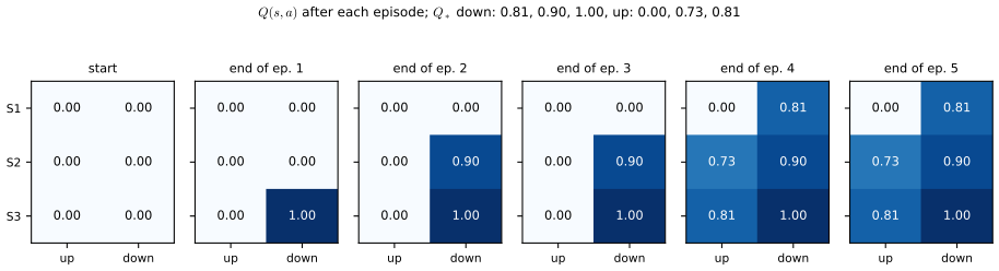
p. 1153, Figure 35.4 Figure 35.4 applies tabular Q-learning with \(\eta=1\) to the 1-D grid world of Figure 34.13 with \(\gamma=0.9\), \(Q\equiv0\) initially. With \(\eta=1\) every update becomes \(Q(s,a)=r+\gamma\max_bQ(s',b)\): the value of the goal is passed back one step per visit. My version uses a random \(\epsilon\)-greedy exploration sequence (\(\epsilon=0.5\)) instead of the book's hand-written one.
35.2.5.2 Double Q-learning
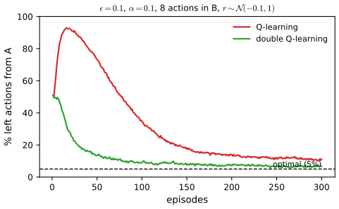
pp. 1153–1154, Figure 35.5 Q-learning suffers from the maximisation bias (the optimiser's curse, Smith and Winkler 2006): \(\E[\max_aX_a]\ge\max_a\E[X_a]\), so acting greedily on noisy scores can pick an action just because noise made it look good. In the MDP of Figure 35.5 the start state \(A\) offers right (reward 0, episode ends) and left (reward 0, then state \(B\)), and from \(B\) many actions end the episode with rewards \(\N(-0.1,1)\). The expected return of going left is \(-0.1\), so left is suboptimal, but the maximum of the noisy estimates at \(B\) is positive, which makes left look attractive. Double Q-learning (Hasselt 2010) keeps two tables \(Q_1,Q_2\) and, on a transition \((s,a,r,s')\), updates \[ Q_1(s,a)\leftarrow Q_1(s,a)+\eta\Bigl[r+\gamma Q_2\bigl(s',\argmax_{a'}Q_1(s',a')\bigr)-Q_1(s,a)\Bigr], \tag{35.13} \] and the same with the roles swapped: one table selects the action, the other evaluates it. Gap 35.9 proves the bias statements; the maximisation-bias demo reruns Figure 35.5 with adjustable noise, step size and number of actions.
Filling the gap 35.9: E[max] ≥ max E, the size of the bias, and why the double estimator removes it pp. 1153–1154, (35.13)
Derivation
The inequality. For every realisation, \(\max_aX_a\ge X_{a'}\) for each fixed \(a'\); taking expectations, \(\E[\max_aX_a]\ge\E[X_{a'}]\), and maximising the right side over \(a'\) gives \(\E[\max_aX_a]\ge\max_a\E[X_a]\) (Jensen's inequality for the convex function max).
The size. For \(n\) independent \(\N(\mu,\sigma^2)\) estimates, \(\E[\max_aX_a]=\mu+\sigma c_n\) with \(c_n=\int x\,n\varphi(x)\Phi(x)^{n-1}\d x\), the mean of the maximum of \(n\) standard normals: \(c_8=1.4236\) (I integrated this numerically and confirmed it by simulation). In Figure 35.5 the estimates \(Q(B,\cdot)\) start at 0 (above the true \(-0.1\)) and are exponential moving averages with step \(\eta\) of independent \(\N(-0.1,1)\) rewards, updated only in the episodes that go left. After they have forgotten the initial value each has variance about \(\sigma^2\eta/(2-\eta)\), a standard deviation of \(0.229\) for \(\eta=0.1\), so \(\max_bQ(B,b)\) has mean about \(-0.1+1.4236\cdot0.229=+0.23\) if every action is updated about equally often; in the simulation the average of \(\max_bQ(B,b)\) is \(+0.10\) after 10 episodes and \(+0.11\) after 25, against \(-0.005\) and \(-0.026\) for the cross-evaluated value of double Q-learning, which is unbiased for the true \(-0.1\) and moves toward it. The bootstrapped target of \(Q(A,\text{left})\) is therefore positive on average, above the value 0 of right, and the agent chooses left far more often than the 5% that \(\epsilon\)-greedy exploration alone produces. The error is corrected only when left is tried, so as left becomes rare the estimates at \(B\) recover slowly: the Q-learning estimate of \(B\) is still \(-0.047\) after 300 episodes (against \(-0.097\) for the double estimator) and the Q-learning curve of the figure is still at 11%.
The double estimator. Let \(X^{(1)},X^{(2)}\) be independent estimates of the same means \(\mu_a\), and \(\hat a=\argmax_aX^{(1)}_a\). Because \(\hat a\) depends only on \(X^{(1)}\), conditionally on it \(\E[X^{(2)}_{\hat a}\given X^{(1)}]=\mu_{\hat a}\), so \(\E[X^{(2)}_{\hat a}]=\E[\mu_{\hat a}]\le\max_a\mu_a\). It never overestimates the maximum of the true means; when all means are equal, as at state \(B\), it is exactly unbiased (\(-0.1\)). The price is a possible small underestimate when the arms differ. Double Q-learning (35.13) applies this to the bootstrap target: table 1 selects \(\argmax Q_1(s',\cdot)\), table 2 supplies its value.
Check. With 8 actions at \(B\): the simulated mean of the maximum of 8 normals matched 1.4236, and the mean of \(X^{(2)}_{\hat a}\) over 400,000 draws was within 0.01 of 0. In the full simulation (3000 runs) Q-learning peaked at 92–93% left actions around episode 16, double Q-learning never exceeded 51% (its starting value), and both ended near the \(\epsilon\)-greedy optimum of 5% (11% and 7% after 300 episodes).
Demo: Q-learning against double Q-learning; preset 2 uses a single action at \(B\) (no bias) and preset 4 a small step size.
35.2.6 Deep Q-network (DQN)
pp. 1154–1156 With function approximation Q-learning is hard to use in practice. The deep Q-network of Mnih et al. (2015) made it work with two heuristics. Experience replay (Lin 1992) stores recent \((s,a,r,s')\) tuples in a buffer \(\D\) and also updates on tuples sampled from it, which uses every transition many times and decorrelates the training data. A target network \(Q_{\bm w^-}\), a frozen copy refreshed every few episodes, supplies the bootstrap targets, so the network does not chase a constantly moving target: \[ \mathcal L_{\mathrm{DQN}}(\bm w)=\E_{(s,a,r,s')\sim\mathrm U(\D)}\Bigl[\bigl(r+\gamma\max_{a'}Q_{\bm w^-}(s',a')-Q_{\bm w}(s,a)\bigr)^2\Bigr]. \tag{35.14} \] Setting \(\bm w^-\leftarrow\bm w\) periodically is an instance of fitted value iteration. Improvements: double DQN (use (35.13) to remove the maximisation bias; Hasselt et al. 2016), prioritised experience replay (sample tuples with probability \(\propto(|\delta|+\varepsilon)^\eta\), where \(\delta\) is the current TD error and \(\eta=0\) is uniform sampling; Schaul et al. 2016), dueling networks (learn \(V_{\bm w}\) and \(A_{\bm w}\) with shared parameters, helpful when many actions have similar values; Wang et al. 2016), and Rainbow (Hessel et al. 2018) which combines these with multi-step returns, distributional RL (predict the distribution of returns, Bellemare et al. 2017) and noisy networks (random weight noise for exploration, Fortunato et al. 2018). Gap 35.10 shows what (35.14) computes.
Filling the gap 35.10: the DQN gradient, and fitted Q-iteration equals value iteration on the empirical model pp. 1154–1156, (35.14)
Derivation
The gradient. With the target network held fixed, \(\nabla_{\bm w}\mathcal L_{\mathrm{DQN}}=-2\,\E_{\mathrm U(\D)}\bigl[\delta^-\nabla_{\bm w}Q_{\bm w}(s,a)\bigr]\), \(\delta^-=r+\gamma\max_{a'}Q_{\bm w^-}(s',a')-Q_{\bm w}(s,a)\): gradient descent on (35.14) is the semi-gradient Q-learning update (35.7, 35.12) averaged over replayed tuples. The replay distribution \(\mathrm U(\D)\) is the data distribution of the behaviour policies, not that of the current greedy policy, so this is an off-policy bootstrapping method of the kind analysed in gap 35.24, and nothing here guarantees convergence; the two heuristics reduce the instability without removing it. Prioritised replay changes the sampling distribution to \(p_i\propto(|\delta_i|+\varepsilon)^\eta\), which weights the loss differently from the uniform expectation; Schaul et al. (2016) correct the bias with importance weights \((|\D|p_i)^{-\beta}\) (not derived in the book).
The tabular case. Let the features be indicators of \((s,a)\) and let each outer iteration fit the network exactly (zero loss on the buffer) before copying \(\bm w^-\leftarrow\bm w\). The minimiser of \(\sum_{i\in\D}(y_i-Q(s_i,a_i))^2\) with targets \(y_i=r_i+\gamma\max_{a'}Q_{k}(s_i',a')\) is the average of the targets over the tuples at each \((s,a)\), so \[ Q_{k+1}(s,a)=\hat R(s,a)+\gamma\sum_{s'}\hat P(s'\given s,a)\max_{a'}Q_k(s',a'), \] with \(\hat R,\hat P\) the empirical mean reward and transition frequencies of the buffer: this is value iteration in the maximum-likelihood MDP (it is the direct method of Section 35.5.1.1 in disguise), and it converges at rate \(\gamma^k\) to the optimal Q-function of the empirical model. The error of the policy found, relative to the true \(Q_*\), is then the estimation error of \(\hat R,\hat P\) compounded over the effective horizon \(1/(1-\gamma)\). I verified numerically on a random 4-state MDP that 200 rounds of tabular fitted Q-iteration on a batch of sampled transitions give exactly (to \(10^{-9}\)) the optimal Q-function of the empirical model.
35.3 Policy-based RL
pp. 1156–1163 Value-based methods are awkward for continuous actions, may diverge under function approximation, and train \(Q\) with a loss that is only indirectly related to the return of the resulting policy. Policy search optimises the parameters of the policy directly for the expected return, and benefits from a value or advantage estimate to reduce variance.
35.3.1 The policy gradient theorem
p. 1157, (35.15)–(35.22) Consider the episodic case (the continuing case with an average-reward criterion is similar). The objective is the expected return of the policy, \[ J(\pi)\triangleq\E_{p_0,\pi}[G_0]=\E_{p_0(s_0)}[V_\pi(s_0)]=\E_{p_0(s_0)\pi(a_0\given s_0)}[Q_\pi(s_0,a_0)]. \tag{35.15} \] For policies \(\pi_{\bm\theta}\), the gradient is \[ \nabla_{\bm\theta}J(\pi_{\bm\theta})=\sum_{t=0}^\infty\gamma^t\E_{p_t(s)}\Bigl[\sum_a\nabla_{\bm\theta}\pi_{\bm\theta}(a\given s)Q_{\pi_{\bm\theta}}(s,a)\Bigr] \tag{35.19} \] \[ =\frac1{1-\gamma}\E_{p^\infty_{\pi_{\bm\theta}}(s)\pi_{\bm\theta}(a\given s)}\bigl[\nabla_{\bm\theta}\log\pi_{\bm\theta}(a\given s)\,Q_{\pi_{\bm\theta}}(s,a)\bigr], \tag{35.20, 35.21} \] the policy gradient theorem (Sutton et al. 1999), where \(p_t(s)\) is the probability of visiting \(s\) at time \(t\) and \(p^\infty_\pi=(1-\gamma)\sum_t\gamma^tp_t\). Note that it does not involve the derivative of the state distribution. A baseline \(b(s)\) can be subtracted for variance reduction (Section 6.3.4.1), \[ \nabla_{\bm\theta}J(\pi_{\bm\theta})=\frac1{1-\gamma}\E_{p^\infty_{\pi_{\bm\theta}}(s)\pi_{\bm\theta}(a\given s)}\bigl[\nabla_{\bm\theta}\log\pi_{\bm\theta}(a\given s)\,(Q_{\pi_{\bm\theta}}(s,a)-b(s))\bigr], \tag{35.22} \] with \(b(s)=V_{\pi_{\bm\theta}}(s)\) a common choice. Gap 35.11 proves (35.19) to (35.21) and writes the gradient in closed form for a tabular softmax policy.
Filling the gap 35.11: proof of the policy gradient theorem, and the tabular softmax gradient p. 1157, (35.16)–(35.21)
Derivation
Assumptions. Finite state and action sets, \(\gamma<1\), bounded rewards, \(\pi_{\bm\theta}(a\given s)\) differentiable in \(\bm\theta\). Then \(V_\pi\) and \(Q_\pi\) are bounded and differentiable.
Unrolling. \(V_\pi(s)=\sum_a\pi(a\given s)Q_\pi(s,a)\) and \(Q_\pi(s,a)=R(s,a)+\gamma\sum_{s'}p(s'\given s,a)V_\pi(s')\). Differentiate the first with the product rule and the second term by term (\(R\) and \(p\) do not depend on \(\bm\theta\)): \[ \nabla V_\pi(s)=\sum_a\nabla\pi(a\given s)Q_\pi(s,a)+\sum_a\pi(a\given s)\nabla Q_\pi(s,a)=\phi(s)+\gamma\sum_{s'}P_\pi(s'\given s)\nabla V_\pi(s'), \] where \(\phi(s)=\sum_a\nabla\pi(a\given s)Q_\pi(s,a)\) and \(P_\pi(s'\given s)=\sum_a\pi(a\given s)p(s'\given s,a)\). This is the linear system \(\nabla V=\phi+\gamma P_\pi\nabla V\) (each component of \(\bm\theta\) separately), whose unique solution is the Neumann series \(\nabla V=\sum_{t\ge0}\gamma^tP_\pi^t\phi\), since the spectral radius of \(\gamma P_\pi\) is at most \(\gamma<1\). Averaging over \(s_0\sim p_0\) and using \((p_0^\T P_\pi^t)(s)=p_t(s)\), \[ \nabla J=\E_{p_0}[\nabla V_\pi(s_0)]=\sum_{t\ge0}\gamma^t\sum_sp_t(s)\phi(s), \] which is (35.19). (The book obtains the same by repeatedly expanding \(\nabla Q_\pi\) as in (35.17, 35.18).)
Discounted visitation and the score function. Since \(\sum_t\gamma^tp_t(s)=p^\infty_\pi(s)/(1-\gamma)\), (35.19) equals \(\frac1{1-\gamma}\sum_sp^\infty_\pi(s)\sum_a\nabla\pi(a\given s)Q_\pi(s,a)\) (35.20); writing \(\nabla\pi=\pi\nabla\log\pi\) inside the sum over actions turns the inner sum into an expectation under \(\pi\): (35.21). The derivative of the state distribution never appears, because \(V_\pi\) was differentiated through the Bellman recursion instead of through the trajectory distribution.
A tabular softmax policy. With \(\pi(a\given s)=\softmax(\bm\theta_s)_a\), \(\partial\pi(a\given s)/\partial\theta_{s,b}=\pi(a\given s)(\ind[a=b]-\pi(b\given s))\), so \(\sum_a\frac{\partial\pi(a\given s)}{\partial\theta_{s,b}}Q_\pi(s,a)=\pi(b\given s)\bigl(Q_\pi(s,b)-V_\pi(s)\bigr)\), and \(\phi\) has no component for other states \(s''\ne s\) at \(\theta_{s,b}\). Using (35.20), \[ \frac{\partial J}{\partial\theta_{s,b}}=\frac{1}{1-\gamma}\,p^\infty_\pi(s)\,\pi(b\given s)\,A_\pi(s,b). \] The gradient is the advantage, weighted by how often the state is visited and by the probability of the action.
The REINFORCE estimator is unbiased. Sampling \(\tau\) from \(\pi\), \(\E[G_t\given s_t,a_t]=Q_\pi(s_t,a_t)\) by the Markov property, and \(\E_{a\sim\pi}[\nabla\log\pi(a\given s)Q_\pi(s,a)]=\sum_a\nabla\pi Q_\pi=\phi(s)\), so \(\E\bigl[\sum_t\gamma^tG_t\nabla\log\pi(a_t\given s_t)\bigr]=\sum_t\gamma^t\sum_sp_t(s)\phi(s)=\nabla J\), the book's (35.24) (the factor \(1/(1-\gamma)\) of (35.21) is already inside the discounted sum over \(t\)). With episodes truncated at \(T\) steps the bias is \(O(\gamma^T)\).
Check. On a random MDP (5 states, 3 actions, \(\gamma=0.9\), random initial distribution and softmax parameters) the closed form agreed with central finite differences of \(J\) to \(2\times10^{-9}\), and the sum over \(t\) in (35.19), computed with 600 terms, reproduced the same gradient to \(10^{-8}\).
35.3.2 REINFORCE
p. 1158, Algorithm 35.2 Applying stochastic gradient ascent to the theorem with a sampled trajectory \(\tau=(s_0,a_0,r_0,\dots,s_T)\), \(s_0\sim p_0\), gives \[ \nabla_{\bm\theta}J(\pi_{\bm\theta})\approx\sum_{t=0}^{T-1}\gamma^tG_t\nabla_{\bm\theta}\log\pi_{\bm\theta}(a_t\given s_t), \tag{35.23, 35.24} \] and, with a baseline, the update \[ \bm\theta\leftarrow\bm\theta+\eta\sum_{t=0}^{T-1}\gamma^t\bigl(G_t-b(s_t)\bigr)\nabla_{\bm\theta}\log\pi_{\bm\theta}(a_t\given s_t), \tag{35.25} \] the REINFORCE algorithm (Williams 1992). If the trajectory return after \(a_t\) beats the baseline the parameters move to make \(a_t\) more likely there, otherwise less likely: good behaviour is reinforced. The baseline can be constant or state dependent; a natural choice is a learned \(V_{\bm w}(s)\), trained for example by Monte Carlo regression, as in Algorithm 35.2.
Algorithm 35.2 (REINFORCE with a value-function baseline)
- Initialise the policy parameters \(\bm\theta\) and the baseline parameters \(\bm w\).
- Repeat: sample an episode \(\tau=(s_0,a_0,r_0,\dots,s_T)\) with \(\pi_{\bm\theta}\) and compute \(G_t\) for \(t=0,\dots,T-1\) from (34.76).
- For \(t=0,\dots,T-1\): \(\delta=G_t-V_{\bm w}(s_t)\); \(\bm w\leftarrow\bm w+\eta_w\,\delta\,\nabla_{\bm w}V_{\bm w}(s_t)\); \(\bm\theta\leftarrow\bm\theta+\eta_\theta\,\gamma^t\delta\,\nabla_{\bm\theta}\log\pi_{\bm\theta}(a_t\given s_t)\).
- Until converged.
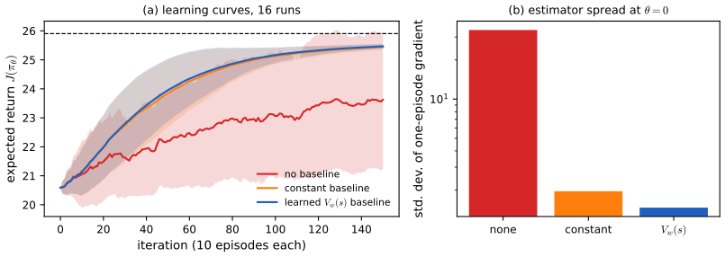
The footnote of the book gives the acronym: REward Increment = Nonnegative Factor × Offset Reinforcement × Characteristic Eligibility; the characteristic eligibility is the score \(\nabla\log\pi\), the offset reinforcement is \(G_t-b(s_t)\), the nonnegative factor is the learning rate. Gap 35.12 proves that baselines leave the estimator unbiased, finds the variance-minimising constant baseline, and Figure 35.13 measures the effect.
Filling the gap 35.12: baselines are unbiased, the variance-optimal baseline, and an experiment pp. 1157–1158, (35.22), (35.25), Algorithm 35.2
Derivation
Unbiasedness. For any function \(b(s)\) of the state (or of the history up to time \(t\) that does not depend on \(a_t\)), \(\E_{a\sim\pi(\cdot\given s)}[b(s)\nabla\log\pi(a\given s)]=b(s)\sum_a\nabla\pi(a\given s)=b(s)\nabla\sum_a\pi(a\given s)=b(s)\nabla1=0\). So subtracting \(b(s_t)\) from \(G_t\) in (35.24) changes the expectation by zero. A baseline that depends on \(a_t\) would not be unbiased.
The best constant baseline. For a single decision (a bandit) with \(\bm u(a)=\nabla\log\pi(a)\) and a reward \(G\), the estimator \(\bm g=(G-b)\bm u\) has mean independent of \(b\), so minimising the total variance \(\E\|\bm g\|^2-\|\E\bm g\|^2\) means minimising \(\E[(G-b)^2\|\bm u\|^2]\), a quadratic in \(b\) with minimiser \[ b^*=\frac{\E[G\,\|\bm u\|^2]}{\E[\|\bm u\|^2]}. \] The optimal baseline is the return weighted by the squared length of the score, not the plain mean return \(V\); they coincide when \(\|\nabla\log\pi\|^2\) is uncorrelated with the return. The state-dependent version has the same form with expectations conditional on \(s\). For a four-armed softmax bandit I minimised the exact variance numerically and recovered \(b^*\) to \(10^{-6}\). The learned \(V_{\bm w}(s)\) of Algorithm 35.2 is therefore near-optimal rather than optimal, and in practice nearly as good.
Experiment. Take a corridor with six states and actions left and right, where the last state pays 1 per step, \(\gamma=0.9\) and a constant offset of 2 is added to every reward; the offset makes every return large and positive, and does not change the optimal policy. At \(\bm\theta=0\) (uniform policy) the exact gradient has norm 0.90, and the standard deviation of a one-episode estimate (total over the 12 coordinates, 20,000 episodes of 80 steps) is 33.8 with no baseline, 2.0 with a constant baseline equal to the mean return from the start, and 1.5 with a state baseline: the first estimator is unbiased but almost all noise. All three means agree with the exact gradient to within sampling error. The learning curves in Figure 35.13 (step size 0.05, batches of 10 episodes) show the consequence: both baselines reach 25.5 of the optimal 25.9 within 150 iterations while the run without baseline is still at 23.6 with a wide band across runs.
Demo: REINFORCE with and without a baseline; preset 1 is the setting of Figure 35.13.
35.3.3 Actor-critic methods
pp. 1158–1160, Algorithms 35.3 and 35.4 An actor-critic method (Barto, Sutton and Anderson 1983) uses a policy gradient with a value function learned by TD in place of Monte Carlo returns: the actor is the policy and the critic the value function. Bootstrapping makes the critic more efficient than Monte Carlo and allows a fully online algorithm that does not wait for the end of an episode. With the one-step TD(0) return \(G_{t:t+1}=r_t+\gamma V_{\bm w}(s_{t+1})\) and the baseline \(V_{\bm w}(s_t)\), (35.25) becomes \[ \bm\theta\leftarrow\bm\theta+\eta\sum_{t=0}^{T-1}\gamma^t\bigl(r_t+\gamma V_{\bm w}(s_{t+1})-V_{\bm w}(s_t)\bigr)\nabla_{\bm\theta}\log\pi_{\bm\theta}(a_t\given s_t). \tag{35.26, 35.27} \]
35.3.3.1 A2C and A3C
p. 1159 The bracket \(r_t+\gamma V_{\bm w}(s_{t+1})-V_{\bm w}(s_t)\) is a single-sample estimate of the advantage \(A(s_t,a_t)=Q(s_t,a_t)-V(s_t)\), so the method is advantage actor-critic (A2C); running actors in parallel with asynchronous updates of shared parameters gives A3C (Mnih et al. 2016).
Algorithm 35.3 (advantage actor-critic, A2C)
- Initialise the actor parameters \(\bm\theta\) and critic parameters \(\bm w\).
- Repeat: sample a starting state \(s_0\); for \(t=0,1,2,\dots\): sample \(a_t\sim\pi_{\bm\theta}(\cdot\given s_t)\); observe \(s_{t+1},r_t\); \(\delta=r_t+\gamma V_{\bm w}(s_{t+1})-V_{\bm w}(s_t)\); \(\bm w\leftarrow\bm w+\eta_w\delta\nabla_{\bm w}V_{\bm w}(s_t)\); \(\bm\theta\leftarrow\bm\theta+\eta_\theta\gamma^t\delta\nabla_{\bm\theta}\log\pi_{\bm\theta}(a_t\given s_t)\).
- Until converged.
35.3.3.2 Eligibility traces
pp. 1159–1160, (35.28)–(35.30), Algorithm 35.4 The \(n\)-step return (35.28) \(G_{t:t+n}=r_t+\gamma r_{t+1}+\dots+\gamma^{n-1}r_{t+n-1}+\gamma^nV_{\bm w}(s_{t+n})\) gives the \(n\)-step advantage \(A^{(n)}_{\pi_{\bm\theta}}(s_t,a_t)=G_{t:t+n}-V_{\bm w}(s_t)\) (35.29). The actual rewards are unbiased but noisy, the value term is biased but low-variance, so \(n\) controls a bias-variance tradeoff. Averaging with weights \(\propto\lambda^n\) as in TD(\(\lambda\)) gives \[ A^{(\lambda)}_{\pi_{\bm\theta}}(s_t,a_t)\triangleq\sum_{\ell=0}^\infty(\gamma\lambda)^\ell\delta_{t+\ell},\qquad\delta_t=r_t+\gamma V_{\bm w}(s_{t+1})-V_{\bm w}(s_t), \tag{35.30} \] which can be implemented with eligibility traces as in Algorithm 35.4; this is generalised advantage estimation (GAE; Schulman et al. 2016). Gap 35.13 collects the two facts needed: the TD error is an unbiased advantage if the critic is exact, and its bias otherwise.
Algorithm 35.4 (actor-critic with eligibility traces)
- Initialise \(\bm\theta,\bm w\). Repeat: set the traces \(\bm z_\theta\leftarrow0\), \(\bm z_w\leftarrow0\); sample \(s_0\).
- For \(t=0,1,2,\dots\): sample \(a_t\sim\pi_{\bm\theta}\); observe \(s_{t+1},r_t\); \(\delta=r_t+\gamma V_{\bm w}(s_{t+1})-V_{\bm w}(s_t)\).
- \(\bm z_w\leftarrow\gamma\lambda_w\bm z_w+\nabla_{\bm w}V_{\bm w}(s_t)\); \(\bm z_\theta\leftarrow\gamma\lambda_\theta\bm z_\theta+\gamma^t\nabla_{\bm\theta}\log\pi_{\bm\theta}(a_t\given s_t)\); \(\bm w\leftarrow\bm w+\eta_w\delta\bm z_w\); \(\bm\theta\leftarrow\bm\theta+\eta_\theta\delta\bm z_\theta\).
- Until converged.
Filling the gap 35.13: the TD error as an advantage estimate, and the bias from an imperfect critic pp. 1159–1160, (35.26)–(35.30)
Derivation
Exact critic. If \(V_{\bm w}=V_\pi\) then \(\E[\delta_t\given s_t=s,a_t=a]=R(s,a)+\gamma\E[V_\pi(s_{t+1})\given s,a]-V_\pi(s)=Q_\pi(s,a)-V_\pi(s)=A_\pi(s,a)\). So (35.27) is the policy gradient with the exact advantage, unbiased for \(\nabla J\) by (35.22) and gap 35.12 (take \(b=V_\pi\) and \(Q_\pi-V_\pi\) as the weight). Also \(\sum_a\pi(a\given s)A_\pi(s,a)=0\), which is why subtracting \(V_\pi\) does not bias the gradient.
Imperfect critic. Write \(e=V_{\bm w}-V_\pi\). Then \[ \E[\delta_t\given s,a]=A_\pi(s,a)+\gamma\,\E[e(s_{t+1})\given s,a]-e(s), \] so the actor receives the advantage plus a bias made of the critic's error at the next state and at the current state. For \(n\)-step advantages the bias is \(\gamma^n\E[e(s_{t+n})\given s_t,a_t]-e(s_t)\) (gap 35.8), which shrinks with \(n\) and \(\gamma\); for \(\lambda\)-weighted advantages the bias is the \((1-\lambda)\)-weighted combination, and \(\lambda=1\) removes it (the Monte Carlo advantage \(G_t-V_{\bm w}(s_t)\) is unbiased for \(A_\pi\) whatever the critic) at the price of the variance of all future rewards. This is the bias-variance tradeoff behind (35.30); the identity \(A^{(\lambda)}=\sum_\ell(\gamma\lambda)^\ell\delta_{t+\ell}\) is the sum of TD errors of gap 35.8 with \(V=V_{\bm w}\). I checked \(\E[\delta\given s,a]=A_\pi\) with the exact value function on a random MDP.
35.3.4 Bound optimization methods
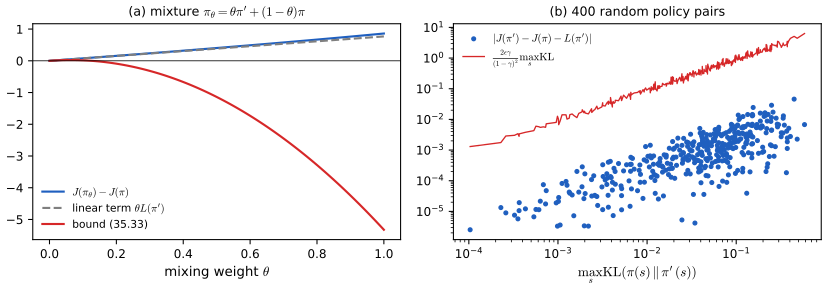
pp. 1160–1162, (35.31)–(35.37) The objective of plain policy gradient need not increase at every step and can collapse if the step is too large. Methods with guaranteed monotone improvement resemble bound optimisation algorithms (Section 6.5). They rest on the performance-difference identity (Kakade and Langford 2002) \[ J(\pi')-J(\pi)=\frac1{1-\gamma}\E_{p^\infty_{\pi'}(s)}\Bigl[\E_{\pi'(a\given s)}[A_\pi(s,a)]\Bigr] \tag{35.31} \] for two arbitrary policies; if \(\E_{\pi'}[A_\pi]\ge0\) at every state then \(J(\pi')\ge J(\pi)\), the policy improvement theorem. With function approximation such a uniformly improving \(\pi'\) may not be representable, and states from \(p^\infty_{\pi'}\) cannot be sampled before \(\pi'\) exists. The remedy is to improve conservatively: with \(\pi_\theta=\theta\pi'+(1-\theta)\pi\), \(J(\pi_\theta)-J(\pi)=\theta L(\pi')+O(\theta^2)\), where the surrogate uses the states of the current policy, \[ L(\pi')\triangleq\frac1{1-\gamma}\E_{p^\infty_\pi(s)}\Bigl[\E_{\pi'(a\given s)}[A_\pi(s,a)]\Bigr]=\frac1{1-\gamma}\E_{p^\infty_\pi(s)\pi(a\given s)}\Bigl[\frac{\pi'(a\given s)}{\pi(a\given s)}A_\pi(s,a)\Bigr]. \tag{35.32} \] Bounding the quadratic remainder gives the conservative policy iteration (CPI) lower bound (Kakade and Langford 2002) \[ J_{\mathrm{CPI}}(\pi_\theta)\triangleq J(\pi)+\theta L(\pi')-\frac{2\epsilon\gamma}{(1-\gamma)^2}\theta^2,\qquad\epsilon=\max_s\bigl|\E_{\pi'(a\given s)}[A_\pi(s,a)]\bigr|, \tag{35.33} \] with \(J(\pi_\theta)\ge J_{\mathrm{CPI}}\). The condition of a small \(\theta\) generalises to a small divergence between \(\pi'\) and \(\pi\): safe policy iteration (Pirotta et al. 2013) uses the maximum total variation, trust region policy optimisation (TRPO; Schulman et al. 2015) the maximum KL divergence, with the bound \[ J_{\mathrm{TRPO}}(\pi')\triangleq J(\pi)+L(\pi')-\frac{\epsilon\gamma}{(1-\gamma)^2}\max_s\KL\bigl(\pi(s)\,\|\,\pi'(s)\bigr),\qquad\epsilon=\max_{s,a}|A_\pi(s,a)|. \tag{35.34} \] In practice this is too conservative; the practical TRPO replaces the maximum KL by an average over \(p^\infty_\pi\) and maximises only \(L\) inside a KL ball, \[ \argmax_{\pi'}L(\pi')\quad\text{s.t.}\quad\E_{p^\infty_\pi(s)}\bigl[\KL(\pi(s)\,\|\,\pi'(s))\bigr]\le\delta. \tag{35.35} \] Gap 35.14 proves (35.31) and (35.33) and gives a complete proof of a bound of the form (35.34) (with the constant I can prove). Figure 35.15 shows the bounds on a random MDP.
Filling the gap 35.14: the performance-difference lemma and the conservative and trust-region lower bounds pp. 1160–1161, (35.31)–(35.34)
Derivation
Performance difference (35.31). Let \(A_\pi(s,a)=R(s,a)+\gamma\E[V_\pi(s')\given s,a]-V_\pi(s)\). Along a trajectory of \(\pi'\), \(\E[r_t+\gamma V_\pi(s_{t+1})-V_\pi(s_t)\given s_t,a_t]=A_\pi(s_t,a_t)\). Summing with weights \(\gamma^t\) (the sum of the \(V_\pi\) terms telescopes: \(\sum_t(\gamma^{t+1}V_\pi(s_{t+1})-\gamma^tV_\pi(s_t))=-V_\pi(s_0)\) since \(\gamma^TV_\pi(s_T)\to0\)), \[ \E_{\tau\sim\pi'}\Bigl[\sum_t\gamma^tA_\pi(s_t,a_t)\Bigr]=\E_{\pi'}\Bigl[\sum_t\gamma^tr_t\Bigr]-\E_{p_0}[V_\pi(s_0)]=J(\pi')-J(\pi). \] The left side is \(\sum_t\gamma^t\E_{p'_t}\E_{\pi'}[A_\pi]=\frac1{1-\gamma}\E_{p^\infty_{\pi'}}\E_{\pi'}[A_\pi]\), which is (35.31). Checked exactly on 300 random MDP policy pairs.
A coupling lemma. Let \(\pi,\pi'\) be policies such that, at each state, the total variation distance \(\TV(\pi(s),\pi'(s))\le\alpha\). Then \(\|p^\infty_{\pi'}-p^\infty_\pi\|_1\le\dfrac{2\gamma\alpha}{1-\gamma(1-\alpha)}\le\dfrac{2\gamma\alpha}{1-\gamma}\). Proof. Run two agents from the same start state. At each step, if their histories agree so far, draw their actions from a maximal coupling of \(\pi(s_t)\) and \(\pi'(s_t)\), which disagree with probability at most \(\alpha\); both then draw the same next state given the same state and action. The histories agree up to time \(t\) with probability at least \((1-\alpha)^t\), so \(\Pr(s_t\ne s_t')\le1-(1-\alpha)^t\), and by the coupling inequality \(\|p'_t-p_t\|_1\le2(1-(1-\alpha)^t)\). Therefore \[ \|p^\infty_{\pi'}-p^\infty_\pi\|_1\le2(1-\gamma)\sum_t\gamma^t\bigl(1-(1-\alpha)^t\bigr)=2\Bigl(1-\frac{1-\gamma}{1-\gamma(1-\alpha)}\Bigr)=\frac{2\gamma\alpha}{1-\gamma(1-\alpha)}. \] For the mixture \(\pi_\theta=\theta\pi'+(1-\theta)\pi\) the same argument with the \(\theta\)-event (use \(\pi'\) with probability \(\theta\) and \(\pi\) otherwise) gives the same bound with \(\alpha=\theta\), because the two agents differ only after a \(\theta\)-event. I checked the bound on mixture paths.
The CPI bound (35.33). Under \(\pi_\theta\), \(\E_{a\sim\pi_\theta}[A_\pi(s,a)]=\theta\E_{\pi'}[A_\pi(s,a)]+(1-\theta)\E_\pi[A_\pi(s,a)]=\theta A'(s)\), with \(A'(s)=\E_{\pi'}[A_\pi(s,\cdot)]\) and \(\E_\pi[A_\pi]=0\). By (35.31), \[ J(\pi_\theta)-J(\pi)=\frac\theta{1-\gamma}\E_{p^\infty_{\pi_\theta}}[A']\ \ge\ \frac\theta{1-\gamma}\E_{p^\infty_\pi}[A']-\frac\theta{1-\gamma}\,\epsilon\,\bigl\|p^\infty_{\pi_\theta}-p^\infty_\pi\bigr\|_1\ \ge\ \theta L(\pi')-\frac{2\epsilon\gamma}{(1-\gamma)^2}\theta^2, \] using \(|\E_pf-\E_qf|\le\|f\|_\infty\|p-q\|_1\) and the coupling lemma with \(\alpha=\theta\). This is (35.33), with the constant of the book. The linear term is the first-order expansion, \(J(\pi_\theta)-J(\pi)=\theta L(\pi')+O(\theta^2)\) as stated.
A trust-region bound of the form (35.34). Let \(\alpha=\max_s\TV(\pi(s),\pi'(s))\), \(\epsilon_A=\max_{s,a}|A_\pi(s,a)|\). Since \(\E_\pi[A_\pi]=0\), \(|A'(s)|=|\E_{\pi'}A_\pi-\E_\pi A_\pi|\le\|A_\pi(s,\cdot)\|_\infty\|\pi'(s)-\pi(s)\|_1\le2\alpha\epsilon_A\). Then, by (35.31) and (35.32), \[ J(\pi')-J(\pi)-L(\pi')=\frac1{1-\gamma}\bigl(\E_{p^\infty_{\pi'}}-\E_{p^\infty_\pi}\bigr)[A']\ \ge\ -\frac{2\alpha\epsilon_A}{1-\gamma}\cdot\frac{2\gamma\alpha}{1-\gamma}=-\frac{4\epsilon_A\gamma\,\alpha^2}{(1-\gamma)^2}, \] and Pinsker's inequality \(\alpha^2\le\tfrac12\max_s\KL(\pi(s)\|\pi'(s))\) gives \[ J(\pi')\ \ge\ J(\pi)+L(\pi')-\frac{2\epsilon_A\gamma}{(1-\gamma)^2}\max_s\KL\bigl(\pi(s)\,\|\,\pi'(s)\bigr). \] This is the form (35.34) with the constant \(2\epsilon\gamma/(1-\gamma)^2\), twice the one printed in the book. I could not derive the book's smaller constant and, equally, I did not find a counterexample to it (hill-climbing over MDPs and policy pairs found only non-negative slack with the book's constant). The version proved here is the one used in the literature (Schulman et al. 2015, with total variation and then Pinsker).
Monotone improvement. Let \(M(\pi')=J(\pi)+L(\pi')-C\max_s\KL(\pi(s)\|\pi'(s))\) be the right side. Then \(M(\pi)=J(\pi)\) (as \(L(\pi)=0\) and the KL vanishes) and \(J(\pi')\ge M(\pi')\) for all \(\pi'\), so \(\pi'=\argmax M\) satisfies \(J(\pi')\ge M(\pi')\ge M(\pi)=J(\pi)\): maximising the lower bound cannot decrease the objective. This is the majorise-minimise argument of Section 6.5 with \(M\) as the surrogate.
Checks. On random 5-state, 3-action MDPs (\(\gamma=0.8\)): (35.31) held to \(10^{-10}\); the CPI bound held for 900 mixture paths; the total variation version and the KL version with constant 2 held on all 300 random policy pairs. On a 3-state MDP with \(\gamma=0.9\), hill climbing for a violation of the book's constant reached a smallest slack of 0.0014 (positive).
pp. 1161–1162, (35.36), (35.37) Section 6.4.2.1 shows that a trust region with a KL penalty is equivalent to natural gradient descent, which matters here because a step of size \(\eta\) in parameter space is not a step of size \(\eta\) in policy space: \[ d_\theta(\bm\theta_1,\bm\theta_2)=d_\theta(\bm\theta_2,\bm\theta_3)\ \not\Rightarrow\ d_\pi(\pi_{\bm\theta_1},\pi_{\bm\theta_2})=d_\pi(\pi_{\bm\theta_2},\pi_{\bm\theta_3}), \tag{35.36} \] with \(d_\theta\) the Euclidean and \(d_\pi\) the KL distance. The natural gradient (approximated by K-FAC, Wu et al. 2017) takes the geometry into account. Instead of a KL constraint one can use the clipped objective of proximal policy optimisation (PPO; Schulman et al. 2017), \[ J_{\mathrm{PPO}}(\pi')\triangleq\frac1{1-\gamma}\E_{p^\infty_\pi(s)\pi(a\given s)}\Bigl[\kappa_\epsilon\Bigl(\frac{\pi'(a\given s)}{\pi(a\given s)}\Bigr)A_\pi(s,a)\Bigr],\qquad\kappa_\epsilon(x)=\clip(x,1-\epsilon,1+\epsilon), \tag{35.37} \] which is simpler and often works better; it can be modified to guarantee monotonic improvement (Wang et al. 2019). Gap 35.15 proves what the section 6.4 result gives here and what the clip does.
Filling the gap 35.15: the KL trust region is a natural-gradient step, equal steps are unequal in policy space, and what the PPO clip does pp. 1161–1162, (35.35)–(35.37)
Derivation
KL is locally the Fisher metric. For a parametric family, \(\KL(\pi_{\bm\theta}\|\pi_{\bm\theta+\bm\Delta})=\tfrac12\bm\Delta^\T F(\bm\theta)\bm\Delta+O(\|\bm\Delta\|^3)\), with \(F(\bm\theta)=\E_{\pi_{\bm\theta}}[\nabla\log\pi_{\bm\theta}\nabla\log\pi_{\bm\theta}^\T]\): expand \(\log\pi_{\bm\theta+\bm\Delta}\) to second order; the first-order term has mean zero because \(\E_\pi[\nabla\log\pi]=0\), and the second-order term gives \(\tfrac12\bm\Delta^\T\E[\nabla^2\log\pi]\bm\Delta\), whose expectation is \(-\tfrac12\bm\Delta^\T F\bm\Delta\) by the information identity. In (35.35) \(F\) is averaged over the states of \(p^\infty_\pi\). (Verified numerically on a three-action softmax: the KL for a step of size \(10^{-3}\) matched \(\tfrac12\bm\Delta^\T F\bm\Delta\).)
The constrained step. By (35.32) and the policy gradient theorem, \(\nabla_{\bm\theta'}L(\pi_{\bm\theta'})|_{\bm\theta'=\bm\theta}=\nabla_{\bm\theta}J(\pi_{\bm\theta})=:\bm g\) (the surrogate has the same gradient as \(J\) at \(\bm\theta\), since \(\E_\pi[A_\pi]=0\)). Linearising \(L\) and using the quadratic KL, (35.35) becomes \(\max_{\bm\Delta}\bm g^\T\bm\Delta\) subject to \(\tfrac12\bm\Delta^\T F\bm\Delta\le\delta\). For \(F\succ0\) the Lagrangian condition \(\bm g=\mu F\bm\Delta\) gives \(\bm\Delta\propto F^{-1}\bm g\), and the constraint fixes the scale: \[ \bm\Delta^*=\sqrt{\frac{2\delta}{\bm g^\T F^{-1}\bm g}}\;F^{-1}\bm g, \] the natural-gradient direction \(F^{-1}\bm g\) with a step length set by \(\delta\) (for a singular \(F\) use the pseudo-inverse). Random feasible steps never beat it in my numerical test (it attained \(\bm g^\T\bm\Delta=0.40233\), the best of 20,000 random steps was lower or equal). So the trust-region view and the natural-gradient view are the same update, which is the statement of Section 6.4.2.1.
(35.36) in an example. For a Bernoulli policy \(\pi_\theta=\sigma(\theta)\) the Euclidean steps \(0\to1\) and \(8\to9\) have the same length, but \(\KL(\sigma(0)\|\sigma(1))=0.1201\) while \(\KL(\sigma(8)\|\sigma(9))=0.00025\): about 500 times smaller, because the policy is nearly deterministic at \(\theta=8\) (the Fisher information is \(\sigma(1-\sigma)\)). The natural gradient divides by this local scale.
The PPO clip. Per sample the objective is \(f(r)=\kappa_\epsilon(r)A\) with \(r=\pi'/\pi\). Its derivative is \(A\) for \(|r-1|<\epsilon\) and \(0\) outside: once the ratio leaves the interval there is no gradient, so there is no incentive to move the ratio further, whichever the sign of \(A\) (I checked this by finite differences). At \(\bm\theta'=\bm\theta\), \(r=1\) and \(\nabla_{\bm\theta'}r=\nabla\log\pi\), so the gradient is exactly the policy gradient estimator (35.22) with the advantage. A remark on (35.37) as printed: the objective of Schulman et al. (2017) is \(\min\bigl(rA,\kappa_\epsilon(r)A\bigr)\), which coincides with \(\kappa_\epsilon(r)A\) except when \(A>0,\ r<1-\epsilon\) or \(A<0,\ r>1+\epsilon\), where the clip-only objective is flat (gradient zero) but the minimum keeps the gradient: the minimum version lets the policy undo a step that has already moved the ratio in the wrong direction, the clip-only version cannot. I confirmed that the two differ exactly in those two cases.
35.3.5 Deterministic policy gradient methods
pp. 1162–1163, (35.38)–(35.45) For a deterministic policy \(a_t=\mu_{\bm\theta}(s_t)\) with continuous states and actions the objective is \[ J(\mu_{\bm\theta})\triangleq\frac1{1-\gamma}\E_{p^\infty_{\mu_{\bm\theta}}(s)}[R(s,\mu_{\bm\theta}(s))], \tag{35.38} \] and the deterministic policy gradient theorem (Silver et al. 2014) gives \[ \nabla_{\bm\theta}J(\mu_{\bm\theta})=\frac1{1-\gamma}\E_{p^\infty_{\mu_{\bm\theta}}(s)}\bigl[\nabla_{\bm\theta}Q_{\mu_{\bm\theta}}(s,\mu_{\bm\theta}(s))\bigr]=\frac1{1-\gamma}\E_{p^\infty_{\mu_{\bm\theta}}(s)}\Bigl[\nabla_{\bm\theta}\mu_{\bm\theta}(s)\,\nabla_aQ_{\mu_{\bm\theta}}(s,a)\big|_{a=\mu_{\bm\theta}(s)}\Bigr]. \tag{35.39, 35.40} \] (The book calls \(\nabla_{\bm\theta}\mu_{\bm\theta}\) an \(M\times N\) matrix; for the product with the \(M\)-vector \(\nabla_aQ\) to be an \(N\)-vector it has to be the \(N\times M\) transposed Jacobian, see Notes on the book.) The integral is over states only, not actions, which lowers the variance, but a deterministic policy does not explore, so an off-policy method is needed that collects data from a stochastic behaviour policy \(\beta\) with stationary state distribution \(p^\infty_\beta\): the objective becomes \(J_b(\mu_{\bm\theta})=\E_{p^\infty_\beta}[V_{\mu_{\bm\theta}}(s)]\) (35.41) with the off-policy gradient (Degris et al. 2012) \[ \nabla_{\bm\theta}J_b(\mu_{\bm\theta})\approx\E_{p^\infty_\beta}\bigl[\nabla_{\bm\theta}\mu_{\bm\theta}(s)\nabla_aQ_{\mu_{\bm\theta}}(s,a)|_{a=\mu_{\bm\theta}(s)}\bigr], \tag{35.42} \] which drops a term containing \(\nabla_{\bm\theta}Q_{\mu_{\bm\theta}}(s,a)\) that is hard to estimate. With a critic learned by TD, \[ \delta=r_t+\gamma Q_{\bm w}(s_{t+1},\mu_{\bm\theta}(s_{t+1}))-Q_{\bm w}(s_t,a_t),\quad\bm w\leftarrow\bm w+\eta_w\delta\nabla_{\bm w}Q_{\bm w}(s_t,a_t),\quad\bm\theta\leftarrow\bm\theta+\eta_\theta\nabla_{\bm\theta}\mu_{\bm\theta}(s_t)\nabla_aQ_{\bm w}(s_t,a)|_{a=\mu_{\bm\theta}(s_t)}, \tag{35.43–35.45} \] which needs no importance sampling in either the actor update (deterministic gradient) or the critic update (Q-learning). If \(Q_{\bm w}\) is linear in \(\bm w\) with features \(\phi(s,a)=\bm a^\T\nabla_{\bm\theta}\mu_{\bm\theta}(s)\) the critic is compatible with the actor and the approximation does not bias the gradient. DDPG (Lillicrap et al. 2016) uses the DQN tricks of Section 35.2.6 with deep networks: the actor minimises \(-Q(s,\pi(s))\) with the state argument frozen by a stop-gradient, the critic minimises the one-step TD loss \((Q(s,a)-(r+\gamma\,\mathrm{sg}(\bar Q(s',\bar\pi(s')))))^2\) with target networks \(\bar Q,\bar\pi\) (exponential moving averages \(\bar\theta=\tau\theta+(1-\tau)\bar\theta\), \(\tau\ll1\)) and samples from a replay buffer. TD3 (Fujimoto et al. 2018) adds double Q-learning and other devices, REDQ (Chen et al. 2021) uses an ensemble of more than two Q networks for a high update-to-data ratio, D4PG (Barth-Maron et al. 2018) adds distributed training and distributional RL, and Amago (Grigsby et al. 2024) shares one transformer sequence model between actor and critic with a loss \(\E[\lambda_0\mathcal L_{\mathrm{TD}}+\lambda_1\mathcal L_{\mathrm{PG}}]\) whose terms are normalised by Pop-Art (van Hasselt et al. 2016: Preserving Outputs Precisely, while Adaptively Rescaling Targets) so that fixed weights can be used. Gap 35.16 proves (35.39) and (35.40).
Filling the gap 35.16: proof of the deterministic policy gradient theorem, with a linear-quadratic check pp. 1162–1163, (35.38)–(35.40)
Derivation
Assumptions. \(R(s,a)\), \(p(s'\given s,a)\) and \(\mu_{\bm\theta}(s)\) are differentiable, with enough regularity to differentiate under the integral. Write \(V=V_{\mu_{\bm\theta}}\) and \(Q(s,a)=R(s,a)+\gamma\int p(s'\given s,a)V(s')\d s'\) (the Q-function of the current policy, in which \(V\) is not differentiated with respect to \(\bm\theta\)).
Unrolling. \(V(s)=Q(s,\mu_{\bm\theta}(s))\). By the chain rule, with \(a=\mu_{\bm\theta}(s)\), \[ \nabla_{\bm\theta}V(s)=\nabla_{\bm\theta}\mu_{\bm\theta}(s)\,\nabla_aQ(s,a)\big|_{a=\mu_{\bm\theta}(s)}+\bigl[\nabla_{\bm\theta}Q(s,a)\bigr]_{a=\mu_{\bm\theta}(s)}, \] where the second term differentiates \(Q\) through \(V\) only: \(\nabla_{\bm\theta}Q(s,a)=\gamma\int p(s'\given s,a)\nabla_{\bm\theta}V(s')\d s'\). Hence \(\nabla V(s)=\psi(s)+\gamma\int p(s'\given s,\mu_{\bm\theta}(s))\nabla V(s')\d s'\) with \(\psi(s)=\nabla_{\bm\theta}\mu_{\bm\theta}(s)\nabla_aQ(s,a)|_{a=\mu_{\bm\theta}(s)}\). This is the same linear equation as in gap 35.11 (with the one-step kernel of the deterministic policy and \(\phi\) replaced by \(\psi\)), so \(\nabla V(s_0)=\sum_t\gamma^t\E[\psi(s_t)\given s_0]\) and, averaging over \(p_0\) and using \(\sum_t\gamma^tp_t=p^\infty/(1-\gamma)\), \[ \nabla_{\bm\theta}J(\mu_{\bm\theta})=\frac1{1-\gamma}\E_{p^\infty_{\mu_{\bm\theta}}}\bigl[\nabla_{\bm\theta}\mu_{\bm\theta}(s)\nabla_aQ(s,a)|_{a=\mu_{\bm\theta}(s)}\bigr], \] which is (35.40); (35.39) is the same with \(\nabla_{\bm\theta}[Q(s,\mu_{\bm\theta}(s))]\) understood as differentiating only through the action. No derivative of the state distribution appears, as in the stochastic theorem.
A closed-form check. Take the scalar system \(s_{t+1}=as_t+bu_t\), reward \(-(qs^2+ru^2)\), policy \(u=\theta s\), initial state \(s_0\sim\N(0,\sigma_0^2)\), and let \(\rho=a+b\theta\) with \(\gamma\rho^2<1\). Then \(V_\theta(s)=-\kappa s^2\) with \(\kappa=(q+r\theta^2)/(1-\gamma\rho^2)\), \(J(\theta)=-\sigma_0^2\kappa(\theta)\), \(Q_\theta(s,u)=-(qs^2+ru^2)-\gamma\kappa(as+bu)^2\), \(\partial_uQ|_{u=\theta s}=-2s[r\theta+\gamma b\kappa\rho]\) and \(\E_{p^\infty}[s^2]=(1-\gamma)\sigma_0^2/(1-\gamma\rho^2)\), so (35.40) gives \[ \frac{\d J}{\d\theta}=-\frac{2\sigma_0^2}{1-\gamma\rho^2}\bigl[r\theta+\gamma b\kappa\rho\bigr]. \] For \(a=0.9\), \(b=0.5\), \(q=1\), \(r=0.2\), \(\gamma=0.9\), \(\sigma_0=1.3\) this agreed with a central finite difference of \(J(\theta)\) to relative error \(10^{-6}\) at \(\theta=-1,-0.6,-0.2,0.1\), and the closed form of \(J(\theta)\) agreed with a direct simulation of 200,000 trajectories (\(-3.127\) against \(-3.120\) at \(\theta=-0.4\), within sampling error). I do not prove the compatibility statement for linear critics, nor that a stochastic policy's gradient tends to (35.40) as the noise vanishes; both are quoted from Silver et al. (2014).
35.3.6 Gradient-free methods
p. 1163 The policy gradient estimator is a zeroth-order gradient (it uses only function values from sampled trajectories), so a derivative-free optimiser (Section 6.7) can be as good: Mania et al. (2018) train linear policies by random search, Salimans et al. (2017) optimise a robot controller with evolution strategies, and Ha and Schmidhuber (2018) use CMA-ES (6.7.5–6.7.6). They scale poorly to many parameters, which is why those controllers are small linear policies.
35.4 Model-based RL
p. 1164 Model-free methods need a great deal of interaction (state-of-the-art Atari agents use millions of frames; a robot-hand controller used the equivalent of 100 years of simulated experience). Model-based RL (MBRL) first learns \(p(s'\given s,a)\) and \(R(s,a)\) and then computes a near-optimal policy with them, so that the agent can "try things out in its imagination". The algorithms for provably efficient exploration of Section 35.1.5.3 (MBIE, UCRL2) are examples, and MBRL links RL with planning (Section 34.6; Sutton 1990). There are many ways to use a model and many kinds of model.
35.4.1 Model predictive control (MPC)
p. 1164, (35.46) Instead of computing a policy for all states in advance, wait until the current state \(s_t\) is known and use the model to find the most promising action sequence over a horizon \(H\), then execute its first action and repeat (receding-horizon control, Mayne and Michalska 1990): \[ \bm a^*_{t:t+H-1}=\argmax_{\bm a_{t:t+H-1}}\E\Bigl[\sum_{h=0}^{H-1}R(s_{t+h},a_{t+h})+\hat V(s_{t+H})\Bigr], \tag{35.46} \] where the expectation is over the state sequences that result from the actions, and \(\hat V\) estimates the reward-to-go at the end of the look-ahead. With a discount, the sum carries \(\gamma^h\) and the terminal term \(\gamma^H\hat V\). Gap 35.17 bounds the loss of this scheme by the error of \(\hat V\) and shows that it improves geometrically with \(H\); Figure 35.16 illustrates it.
Filling the gap 35.17: the suboptimality of H-step lookahead with a terminal value; admissibility of A* pp. 1164–1165, (35.46)
Derivation
Setting. Discounted MDP with known model, optimality operator \(T_*\) and optimal value \(V_*\). The first action chosen by (35.46) (with discounting) maximises \(Q_H(s,a)=R(s,a)+\gamma\sum_{s'}p(s'\given s,a)U(s')\) with \(U=(T_*)^{H-1}\hat V\): the inner \(H-1\) steps of the look-ahead choose the best continuation, which is \(H-1\) applications of the Bellman optimality backup to \(\hat V\). So the MPC policy \(\pi_H\) is the greedy policy for \(U\), i.e. \(T_{\pi_H}U=T_*U\).
Greedy policies for an approximate value. Let \(\pi\) be greedy for a function \(U\). Then \(V_\pi-V_*=T_\pi V_\pi-T_*V_*=(T_\pi V_\pi-T_\pi U)+(T_\pi U-T_*U)+(T_*U-T_*V_*)\). The middle term is 0; the first has norm at most \(\gamma\|V_\pi-U\|_\infty\le\gamma(\|V_\pi-V_*\|_\infty+\|V_*-U\|_\infty)\); the last at most \(\gamma\|U-V_*\|_\infty\). Hence \((1-\gamma)\|V_\pi-V_*\|_\infty\le2\gamma\|U-V_*\|_\infty\): \[ \|V_\pi-V_*\|_\infty\le\frac{2\gamma}{1-\gamma}\|U-V_*\|_\infty. \] The MPC bound. \(T_*\) is a \(\gamma\)-contraction with fixed point \(V_*\), so \(\|U-V_*\|_\infty=\|T_*^{H-1}\hat V-T_*^{H-1}V_*\|_\infty\le\gamma^{H-1}\|\hat V-V_*\|_\infty\), and therefore \[ \|V_{\pi_H}-V_*\|_\infty\le\frac{2\gamma^H}{1-\gamma}\|\hat V-V_*\|_\infty. \] The error of the terminal value is multiplied by \(\gamma^H\): a longer look-ahead buys accuracy geometrically, and with an exact terminal value (\(\hat V=V_*\)) even \(H=1\) is optimal. Without a terminal value (\(\hat V=0\)) the loss decays like \(\gamma^H\|V_*\|\). I verified the bound on 40 random MDPs, horizons 1, 2, 4, 7 and random value errors.
Example. On the stochastic grid world (goal \(+1\), pit \(-1\), slip probability 0.2, step cost 0.04, \(\gamma=0.9\); \(\|V_*\|_\infty=0.93\)) with \(\hat V=0\) the loss is 0.77, 0.45, 0.28, 0.20 for \(H=1,\dots,4\) and exactly 0 for \(H\ge5\): the MPC policy is optimal once the look-ahead sees the goal from the farthest cell (the bound, 16.7 at \(H=1\) down to 11.0 at \(H=5\), is valid but loose). With \(\hat V=0.7V_*\) the loss is 0.025 for \(H=1,2,3\), 0.012 at \(H=4\), and 0 from \(H=5\).
A* (Section 35.4.1.1). In a deterministic shortest-path problem with step costs \(c\ge0\), let \(g(n)\) be the cost so far, \(h^*(n)\) the true cost-to-go and \(h\) an admissible heuristic, \(h\le h^*\). A* expands the frontier node with the smallest \(f=g+h\). Suppose it pops a goal with \(f=g>C^*\) (the optimal cost). Some node \(n\) on an optimal path is still on the frontier, with \(g(n)=g^*(n)\) (its predecessors on the optimal path were expanded), so \(f(n)=g^*(n)+h(n)\le g^*(n)+h^*(n)=C^*<g\), and \(n\) would have been popped before the goal: a contradiction. So the first goal popped has cost \(C^*\), and an admissible heuristic never prunes an optimal path. (In the maximising-reward language of the book, admissibility means \(\hat V\ge V_*\), an upper bound.) On 30 random \(12\times12\) grid mazes, A* with the Manhattan-distance heuristic returned the same optimal cost as Dijkstra's algorithm and never expanded more nodes.
Monte Carlo tree search (Section 35.4.1.2) is a search guided by a UCB rule at each tree node (gap 34.17) whose leaf values are learned instead of hand designed; AlphaGo, AlphaZero (known model) and MuZero (learned model) use it. I do not analyse it here.
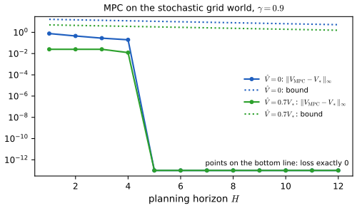
35.4.1.1 Heuristic search
pp. 1164–1165, Figure 35.6 With finite state and action spaces (35.46) can be solved exactly, at a cost that is exponential in \(H\), unless unpromising trajectories are pruned. In a discrete, deterministic MDP where maximising reward means finding a shortest path to a goal, one expands the successors of the current state, guided by a heuristic function (best-first search; Figure 35.6 illustrates a search tree). A heuristic that is an optimistic bound on the distance to the goal is admissible; if the aim is to maximise reward, it must be an upper bound on the value function. Admissibility guarantees that no optimal part of the search space is pruned, and the algorithm is then A* search, which is optimal (gap 35.17; Pearl 1984, Russell and Norvig 2019).
35.4.1.2 Monte Carlo tree search (MCTS)
p. 1165 MCTS is like heuristic search but learns a value function for each state it visits instead of using a hand-designed heuristic (Munos 2014), and it is inspired by UCB for bandits (34.4.5), applied to general sequential problems including MDPs (Kocsis and Szepesvari 2006). It forms the basis of AlphaGo and AlphaZero (Silver et al. 2016, 2018: expert-level Go, chess and shogi with a known model), of MuZero (Schrittwieser et al. 2020) and Stochastic MuZero (Antonoglou et al. 2022), which learn the model, and has been applied to sequential experiment design such as molecule construction (Segler et al. 2018). The action-value functions at the nodes are represented by deep networks and trained with TD methods (Section 35.2).
35.4.1.3 Trajectory optimization for continuous actions
pp. 1165–1166 With continuous actions (35.46) is a nonlinear program in \(\bm a_{t:t+H-1}\). If the dynamics are linear and the reward is a negative quadratic cost the optimal action sequence is available in closed form (the linear-quadratic-Gaussian, LQG, controller). In general it is solved numerically by shooting or collocation, iteratively improving an initial action sequence. Differential dynamic programming (DDP; Jacobson and Mayne 1970, Todorov and Li 2005) linearises the dynamics and forms a local quadratic approximation of the reward around a reference trajectory, solves that LQG problem exactly to get a new trajectory, and repeats. Black-box alternatives such as the cross-entropy method (Section 6.7.5) also work. Gap 35.18 derives the closed-form linear-quadratic solution.
Filling the gap 35.18: the finite-horizon Riccati recursion, and why Gaussian noise does not change the controller pp. 1165–1166
Derivation
Problem. Minimise the cost \(\sum_{t=0}^{T-1}(\bm x_t^\T Q\bm x_t+\bm u_t^\T R\bm u_t)+\bm x_T^\T Q_T\bm x_T\) (the negative of a quadratic reward) subject to \(\bm x_{t+1}=A\bm x_t+B\bm u_t\), with \(Q,Q_T\succeq0\) and \(R\succ0\).
Backward induction. Let \(V_t(\bm x)\) be the optimal cost-to-go. \(V_T(\bm x)=\bm x^\T Q_T\bm x\). Suppose \(V_{t+1}(\bm x)=\bm x^\T P_{t+1}\bm x\) with \(P_{t+1}\succeq0\). Then \[ V_t(\bm x)=\min_{\bm u}\ \bm x^\T Q\bm x+\bm u^\T R\bm u+(A\bm x+B\bm u)^\T P_{t+1}(A\bm x+B\bm u). \] The function is strictly convex in \(\bm u\) (the Hessian is \(2(R+B^\T P_{t+1}B)\succ0\)); setting the gradient to zero, \((R+B^\T P_{t+1}B)\bm u=-B^\T P_{t+1}A\bm x\), so \(\bm u^*_t=-K_t\bm x\) with \(K_t=(R+B^\T P_{t+1}B)^{-1}B^\T P_{t+1}A\). Substituting, \[ V_t(\bm x)=\bm x^\T P_t\bm x,\qquad P_t=Q+A^\T P_{t+1}A-A^\T P_{t+1}B(R+B^\T P_{t+1}B)^{-1}B^\T P_{t+1}A=Q+A^\T P_{t+1}(A-BK_t)\succeq0, \] which closes the induction. The optimal control is a time-varying linear feedback, and the optimal cost from \(\bm x_0\) is \(\bm x_0^\T P_0\bm x_0\). As \(T\to\infty\) the matrices \(P_t\) converge to the solution of the discrete algebraic Riccati equation and \(K_t\) to a constant gain (when the system is stabilisable and detectable).
Additive Gaussian noise. Let \(\bm x_{t+1}=A\bm x_t+B\bm u_t+\bm w_t\) with \(\bm w_t\sim\N(0,W)\) independent. Suppose \(V_{t+1}(\bm x)=\bm x^\T P_{t+1}\bm x+c_{t+1}\). Then \(\E[(A\bm x+B\bm u+\bm w)^\T P_{t+1}(A\bm x+B\bm u+\bm w)]=(A\bm x+B\bm u)^\T P_{t+1}(A\bm x+B\bm u)+\operatorname{tr}(P_{t+1}W)\) because \(\E\bm w=0\): the noise adds a constant that does not depend on \(\bm u\), so the minimiser is unchanged and \(V_t(\bm x)=\bm x^\T P_t\bm x+c_t\), \(c_t=c_{t+1}+\operatorname{tr}(P_{t+1}W)\). Hence the optimal feedback gains are the same as without noise (certainty equivalence) and the optimal expected cost is \(\bm x_0^\T P_0\bm x_0+\sum_{t=1}^T\operatorname{tr}(P_tW)\). If the state is only observed through noise, the same gains are applied to the Kalman-filter estimate (the separation principle of LQG, which I do not prove here).
Checks. For a double integrator (\(A=\begin{pmatrix}1&0.1\\0&1\end{pmatrix}\), \(B=(0,0.1)^\T\), \(Q=\diag(1,0.1)\), \(R=0.05\), \(Q_T=\diag(2,0.5)\), \(T=5\), \(\bm x_0=(1,-0.5)\)) the recursion gives the cost \(5.35125018\), equal to the cost found by minimising directly over the five actions with BFGS (\(5.35125018\)), with first action \(-K_0\bm x_0\). For a horizon of 400 steps the gain at \(t=0\) matches the discrete algebraic Riccati solution to \(10^{-8}\). With noise covariance \(W=\diag(0.01,0.02)\), a simulation of 400,000 trajectories gave the average cost \(5.6216\) against the formula \(5.6206\), and gains inflated by 30% gave the larger \(5.6318\).
35.4.2 Combining model-based and model-free
p. 1166 MPC chooses each action with the model, which can be slow and suffers when the model is wrong. The learned model can instead be used to reduce the sample complexity of learning a policy. In Dyna (Sutton 1990) rollouts from the model produce "hallucinated" data on which a policy or Q-function is trained; Janner et al. (2019) generate short rollouts from previously visited real states so that the model only needs to extrapolate locally. Weber et al. (2017) use the hidden states of a model that predicts future states and rewards as extra context for a policy-based learner (imagination-augmented agents), which can help with partial observability; Jaderberg et al. (2017) train a model to predict future rewards and auxiliary signals, which helps when rewards are sparse or absent.
35.4.3 MBRL using Gaussian processes
pp. 1166–1168 For low-dimensional continuous control problems, such as arise in robotics, a flexible and sample-efficient model is a Gaussian process (Chapter 18). I write \(\bm s,\bm a\) for the vectors.
35.4.3.1 PILCO
pp. 1166–1167, Figure 35.7 PILCO (probabilistic inference for learning control; Deisenroth and Rasmussen 2011, Deisenroth et al. 2015) assumes \(\bm s_{t+1}=f(\bm s_t,\bm a_t)+\bm\epsilon_t\), \(\bm\epsilon_t\sim\N(0,\Sigma)\), with \(f\) unknown and continuous (modelling the residual \(\bm s_{t+1}=\bm s_t+f(\bm s_t,\bm a_t)+\bm\epsilon_t\) often works better). It fits a GP to a few initial random trajectories, then generates "fantasy" rollouts of length \(T\) to evaluate the expected cost of the current policy, \(J(\pi_{\bm\theta})=\sum_{t=1}^T\E_{\bm a_t\sim\pi_{\bm\theta}}[c(\bm s_t)]\) with \(\bm s_0\sim p_0\). If the state distribution at each step is approximated by a Gaussian, this function and its gradient with respect to \(\bm\theta\) can be computed deterministically, because a Gaussian belief can be propagated through the GP model by moment matching; deterministic batch optimisers such as Levenberg-Marquardt then replace stochastic gradient descent. The method is data-efficient enough for real robots (Figure 35.7: a cart-pole swing-up learned from 17.5 seconds of interaction with an RBF controller of 50 basis functions and 305 parameters, 7 trials; a block-stacking task with a low-cost 6-degree-of-freedom arm learned from 230 seconds with a linear policy, 10 trials). The figure shows photographs and has nothing to compute; gap 35.19 derives the Gaussian moments that make the propagation possible.
Filling the gap 35.19: a GP prediction at a Gaussian input has closed-form moments pp. 1166–1167
Derivation
Setting. The squared-exponential kernel \(k(\bm a,\bm b)=\alpha^2\exp\bigl(-\tfrac12(\bm a-\bm b)^\T\Lambda^{-1}(\bm a-\bm b)\bigr)\), \(\Lambda=\diag(\ell_1^2,\dots,\ell_D^2)\); training inputs \(X=(\bm x_1,\dots,\bm x_n)\), targets \(\bm y\), noise variance \(\sigma_n^2\); the posterior mean is \(m(\bm x)=\sum_i\beta_ik(\bm x_i,\bm x)\) with \(\bm\beta=(K+\sigma_n^2I)^{-1}\bm y\). Let the test input be uncertain, \(\bm x\sim\N(\bm\mu,\Sigma)\). We want \(\E[m(\bm x)]\) and \(\E[m(\bm x)^2]\).
The Gaussian product identity. \(\int\N(\bm x\given\bm a,A)\N(\bm x\given\bm b,B)\d\bm x=\N(\bm a\given\bm b,A+B)\). The kernel is an unnormalised Gaussian: \(k(\bm x_i,\bm x)=\alpha^2(2\pi)^{D/2}|\Lambda|^{1/2}\N(\bm x\given\bm x_i,\Lambda)\). Hence \[ q_i:=\E[k(\bm x_i,\bm x)]=\alpha^2(2\pi)^{D/2}|\Lambda|^{1/2}\N(\bm x_i\given\bm\mu,\Sigma+\Lambda)=\alpha^2\,|I+\Sigma\Lambda^{-1}|^{-1/2}\exp\bigl(-\tfrac12(\bm x_i-\bm\mu)^\T(\Sigma+\Lambda)^{-1}(\bm x_i-\bm\mu)\bigr), \] using \(|\Sigma+\Lambda|=|\Lambda||I+\Lambda^{-1}\Sigma|\). Therefore \(\E[m(\bm x)]=\bm\beta^\T\bm q\).
Second moment. Completing the square in the product of two kernels, with \(\bm z_{ij}=(\bm x_i+\bm x_j)/2\): \[ k(\bm x_i,\bm x)k(\bm x_j,\bm x)=\alpha^4\exp\bigl(-\tfrac14(\bm x_i-\bm x_j)^\T\Lambda^{-1}(\bm x_i-\bm x_j)\bigr)\exp\bigl(-(\bm x-\bm z_{ij})^\T\Lambda^{-1}(\bm x-\bm z_{ij})\bigr), \] and the last factor is \((2\pi)^{D/2}|\Lambda/2|^{1/2}\N(\bm x\given\bm z_{ij},\Lambda/2)\). By the product identity, \[ Q_{ij}:=\E[k(\bm x_i,\bm x)k(\bm x_j,\bm x)]=\alpha^4e^{-\frac14(\bm x_i-\bm x_j)^\T\Lambda^{-1}(\bm x_i-\bm x_j)}\,|I+2\Sigma\Lambda^{-1}|^{-1/2}\exp\bigl(-\tfrac12(\bm z_{ij}-\bm\mu)^\T(\Sigma+\Lambda/2)^{-1}(\bm z_{ij}-\bm\mu)\bigr), \] and \(\E[m(\bm x)^2]=\bm\beta^\T Q\bm\beta\). The predictive variance of \(f(\bm x)\) adds the expected GP variance \(\E[\sigma^2(\bm x)]\), which is computed in the same way, and PILCO approximates the output distribution by the Gaussian with these first two moments (moment matching). The numbers are exact for the mean function of the GP, so the deterministic propagation through the fitted GP has no sampling noise.
Check. For seven random two-dimensional training points, \(\bm\mu=(0.2,-0.1)\), \(\Sigma=\begin{pmatrix}0.3&0.1\\0.1&0.2\end{pmatrix}\), \(\bm\ell^2=(0.5,0.8)\), \(\alpha^2=1.3\): \(\bm\beta^\T\bm q=0.07587\) against a Monte Carlo average of 0.07582 and \(\bm\beta^\T Q\bm\beta=0.31540\) against 0.31543 (1.5 million samples; within five standard errors in both cases).
35.4.3.2 GP-MPC
pp. 1167–1168 GP-MPC (Kamthe and Deisenroth 2018) combines the GP model with MPC. It uses an open-loop sequence of actions \(\bm a_{t:t+H-1}\), propagates a Gaussian approximation of \(p(\bm s_{t+1:t+H}\given\bm a_{t:t+H-1},\bm s_t)\) by moment matching, computes the expected reward and its gradient with respect to the actions deterministically, solves (35.46), executes the first action and repeats. It handles constraints more easily than PILCO, and is more data-efficient because it updates the GP after every step rather than after each trajectory.
35.4.4 MBRL using DNNs
p. 1168 GPs scale poorly to large data sets and high-dimensional inputs; deep networks scale well but do not naturally quantify uncertainty, which can make MPC fail. Section 17.1 discusses uncertainty for networks. Deep PILCO uses MC dropout (17.3.1; Gal et al. 2016), and probabilistic ensembles with trajectory sampling (PETS; Chua et al. 2018) use a deep ensemble (17.3.9). These stochastic models give a high variance in the predicted return, which makes the choice of the best action by MPC hard. The variance of the comparison can be reduced by the common random number trick, a standard variance-reduction device in simulation: all rollouts share the same random seeds, so that differences in \(J(\pi_{\bm\theta})\) are attributable to \(\bm\theta\); this is used in PEGASUS (Policy Evaluation-of-Goodness And Search Using Scenarios; Ng and Jordan 2000) and in later model-based work. Gap 35.20 explains why it works.
Filling the gap 35.20: common random numbers reduce the variance of a comparison p. 1168
Derivation
Let \(\hat J(\bm\theta)=g(\bm\theta,\bm U)\) be the average return of rollouts driven by random numbers \(\bm U\) (the uniforms behind action sampling and, for a stochastic model, the transitions). Each \(\hat J(\bm\theta_i)\) has the same marginal distribution whether or not the random numbers are shared, so \(\E[\hat J(\bm\theta_2)-\hat J(\bm\theta_1)]\) is the same. For the variance of the difference, \[ \var\bigl(\hat J(\bm\theta_2)-\hat J(\bm\theta_1)\bigr)=\var\hat J(\bm\theta_1)+\var\hat J(\bm\theta_2)-2\cov\bigl(\hat J(\bm\theta_1),\hat J(\bm\theta_2)\bigr). \] Independent random numbers give zero covariance. With shared \(\bm U\), the covariance is nonnegative whenever both \(g(\bm\theta_1,\cdot)\) and \(g(\bm\theta_2,\cdot)\) are nondecreasing in each coordinate of \(\bm U\) (the Harris-FKG association inequality for independent coordinates), as is the case when a larger uniform means a luckier draw for both policies; in general policies that behave similarly are positively correlated, and the variance of the difference falls by the covariance term. PEGASUS goes one step further: with the scenarios fixed, \(\hat J(\bm\theta)\) is a deterministic function of \(\bm\theta\), so ordinary deterministic optimisation can be used, at the price of overfitting to the chosen scenarios.
Check. For a six-state corridor and two softmax policies, 20 rollouts of 40 steps each, repeated 600 times: the variance of the estimated difference was 0.0180 with shared random numbers against 0.0712 with independent ones, with the same mean.
35.4.5 MBRL using latent-variable models
pp. 1168–1170 When the states are images, predicting dynamics in the observation space is hard; latent-variable models predict in a compact latent space instead.
35.4.5.1 World models
pp. 1168–1169, Figure 35.8 Ha and Schmidhuber (2018) learn a generative model of two simple video games (a racing game and a VizDoom-like environment) and train a policy entirely inside it (Figure 35.8, an architecture sketch). First, random experience is used to fit a VAE (Chapter 21) that reduces a \(64\times64\times3\) image to a latent \(\bm z_t\in\R^{64}\). Next an RNN with a mixture-density-network output predicts \(p(\bm z_{t+1}\given\bm z_t,\bm a_t,\bm h_t)\), with \(\bm h_t\) the deterministic RNN state and a 3-dimensional continuous action. Finally a small controller acts on \([\bm z_t,\bm h_t]\); it is linear (\((32+256)\times3+3=867\) parameters), trained with CMA-ES (Section 35.3.6; 6.7.6) because a derivative-free optimiser works for so few parameters. The VAE (4.3 M parameters) and MDN-RNN (422 k) are trained without supervision from random rollouts, so sample efficiency is less critical for them. The controller can even be trained in "dream mode", feeding the decoder's images back as inputs and predicting the reward, but this may fail: the model may underfit task-relevant features and memorise irrelevant ones, and the controller can exploit model errors like an adversarial attack. Raising the variance of the model's predictions with a temperature \(\tau\) forces the controller to be robust, similar to domain randomisation for sim-to-real transfer.
35.4.5.2 PlaNet and Dreamer
p. 1170, Figure 35.9 On harder problems the model and controller must be trained iteratively so that the model sees data from the controller. PlaNet (Hafner et al. 2019) treats the task as a POMDP with latent states \(\bm z_t\), observations \(\bm s_t\), actions and rewards. It fits a recurrent state-space model \(p(\bm z_t\given\bm z_{t-1},\bm a_{t-1})p(\bm s_t\given\bm z_t)p(r_t\given\bm z_t)\) (Section 29.13.2) by variational inference with \(q(\bm z_t\given\bm s_{1:t},\bm a_{1:t-1})\), uses the inference model to compute the current belief, and then the cross-entropy method to find the best action sequence of the next \(H\) steps in latent space, executes its first action, updates the model and repeats; "latent overshooting" (Section 29.13.3) trains the dynamics for long horizons. PlaNet outperforms the model-free A3C and D4PG on image-based control (Figure 35.9 shows the six tasks), but is computationally costly (CEM with 1000 samples and 10 iterations for horizon 12 needs 120,000 model evaluations per action). Differentiable CEM in a latent space of action sequences (Amos and Yarats 2020) is much faster, and fine-tuning with PPO closes the gap. Dreamer (Hafner et al. 2020) replaces the online planner with a policy network \(\pi(a_t\given z_t)\) trained by gradient-based actor-critic in latent space: the generative model is trained by maximising the ELBO, the policy to maximise the return predicted by the value function, the value function to minimise the squared error to the TD(\(\lambda\)) estimate (Section 35.2.3). It does better than PlaNet, presumably because the policy optimises the long-term return instead of relying on a short-horizon rollout.
35.4.6 Robustness to model errors
p. 1171 The main difficulty of MBRL is that model errors produce poor policies through distribution shift (Section 19.2): the model is trained on states visited by the behaviour policy, then used to find a policy that visits other states, where the model may be wrong. The model must generalise robustly or at least quantify its uncertainty (Section 19.3); the book points to a number of recent papers on this question. The problem is related to the off-policy learning of the next section.
35.5 Off-policy learning
p. 1171 Off-policy methods such as Q-learning do not need the training data to come from the policy they evaluate or improve, so they can reuse data from other policies, and they suit domains where trying a new policy is costly or risky. The difficulty is that the data distribution differs from the desired one: the visit probability of a state at time \(t\) depends on the policy as well as on the MDP, so if the trajectories come from \(\pi'\), averaging their rewards estimates \(J(\pi')\), not \(J(\pi)\). The mismatch must be corrected, as in covariate shift for supervised learning (Section 19.5.2) and in causal effect estimation (Chapter 36). Off-policy data can also make a bootstrapping algorithm unstable (Section 35.5.3). Off-policy learning is closely related to offline RL, which stresses that the data are static and no new interaction is allowed (Lagoudakis and Parr 2003, Ernst et al. 2005, Levine et al. 2020). Most methods simplify to the contextual bandit (Section 34.4) and have been used in industrial bandit applications.
35.5.1 Basic techniques
pp. 1171–1175 The data are trajectories \(\D=\{\tau^{(i)}\}_{i\le n}\), with actions chosen by a behaviour policy \(\pi_b\) that differs from the target policy \(\pi_e\) being evaluated or improved; \(\pi_b\) is known or unknown (behaviour-agnostic setting).
35.5.1.1 Direct method
p. 1172 Estimate the reward and transition models \(\hat R,\hat P\) by regression and density estimation (Section 35.4) and apply an on-policy method to the simulated data (the regression or plug-in estimator). It is natural and sometimes effective, but small model errors compound over long horizons (or when \(\gamma\) is near 1), the agent may overfit the model's errors, and learning \(\hat P\) accurately is hard (Section 35.4.6). The exact tabular version is fitted Q-iteration of gap 35.10.
35.5.1.2 Importance sampling
pp. 1172–1173, (35.47)–(35.50) Importance sampling (IS; Section 11.5) corrects the distribution mismatch. For a fixed horizon \(T\) the estimator of the target value is (Precup et al. 2000) \[ \hat J_{\mathrm{IS}}(\pi_e)\triangleq\frac1n\sum_{i=1}^n\frac{p(\tau^{(i)}\given\pi_e)}{p(\tau^{(i)}\given\pi_b)}\sum_{t=0}^{T-1}\gamma^tr^{(i)}_t, \tag{35.47} \] which is unbiased, \(\E_{\pi_b}[\hat J_{\mathrm{IS}}(\pi_e)]=J(\pi_e)\), whenever \(p(\tau\given\pi_b)>0\) wherever \(p(\tau\given\pi_e)>0\). The ratio does not involve the unknown MDP models, because they cancel, \[ \frac{p(\tau\given\pi_e)}{p(\tau\given\pi_b)}=\frac{p(s_0)\prod_{t=0}^{T-1}\pi_e(a_t\given s_t)p(s_{t+1}\given s_t,a_t)p_R(r_t\given s_t,a_t,s_{t+1})}{p(s_0)\prod_{t=0}^{T-1}\pi_b(a_t\given s_t)p(s_{t+1}\given s_t,a_t)p_R(r_t\given s_t,a_t,s_{t+1})}=\prod_{t=0}^{T-1}\frac{\pi_e(a_t\given s_t)}{\pi_b(a_t\given s_t)}, \tag{35.48} \] so IS only needs the two policies. If \(\pi_b\) is unknown it can be estimated from \(\D\) (by logistic regression or a network) and \(\hat\pi_b\) used in the ratio. Write \(\rho_t=\pi_e(a_t\given s_t)/\pi_b(a_t\given s_t)\). The estimator can have a very large variance (the ratio can be arbitrarily large). The per-decision variant uses the fact that \(r_t\) is independent of the trajectory after time \(t\) (Section 11.6.2), \[ \hat J_{\mathrm{PDIS}}(\pi_e)\triangleq\frac1n\sum_{i=1}^n\sum_{t=0}^{T-1}\Bigl(\prod_{t'\le t}\rho_{t'}(\tau^{(i)})\Bigr)\gamma^tr^{(i)}_t, \tag{35.49} \] and there are self-normalised and truncated variants that reduce the variance at the price of a small bias (Liu et al. 2018). To improve a policy against (35.15), one cannot simply reuse (35.48) (the problem of Section 35.5.2); an approximation averages over the behaviour state distribution, \(J_b(\pi_{\bm\theta})\triangleq\E_{p^\infty_\beta(s)}[V_\pi(s)]\) (35.50), whose gradient, ignoring \(\nabla_{\bm\theta}Q_\pi\) (Degris et al. 2012), is a one-step importance-corrected policy gradient \(\E_{p^\infty_\beta(s)\beta(a\given s)}\bigl[\frac{\pi_{\bm\theta}(a\given s)}{\beta(a\given s)}\nabla_{\bm\theta}\log\pi_{\bm\theta}(a\given s)Q_\pi(s,a)\bigr]\). In the tabular case one policy \(\pi_*\) is optimal in every state (Section 34.5.5), so \(J_b\) and \(J\) are maximised together as long as the behaviour policy covers all states, and the same holds when the function class is rich enough (for example the Retrace algorithm, Munos et al. 2016); for parametric families that uniform optimality is lost and the state distribution affects the solution. Gap 35.21 proves (35.47) to (35.49).
Filling the gap 35.21: importance sampling and per-decision importance sampling are unbiased pp. 1172–1173, (35.47)–(35.49)
Derivation
The ratio (35.48). The probability of a trajectory under a policy is the product of the initial distribution, the policy terms, and the dynamics and reward terms. Dynamics and rewards are the same for both policies (they belong to the environment), so they cancel in the ratio, leaving the product of the per-step policy ratios \(\prod_t\rho_t\).
Unbiasedness of IS. Let \(G(\tau)=\sum_t\gamma^tr_t\). If \(p(\tau\given\pi_b)>0\) wherever \(p(\tau\given\pi_e)>0\) (positive-support, or "coverage", condition), then \[ \E_{\tau\sim\pi_b}\Bigl[\frac{p(\tau\given\pi_e)}{p(\tau\given\pi_b)}G(\tau)\Bigr]=\sum_{\tau:\,p(\tau\given\pi_b)>0}p(\tau\given\pi_e)G(\tau)=\E_{\tau\sim\pi_e}[G(\tau)]=J(\pi_e). \] Without coverage the estimator is biased downwards for positive rewards, with no way to detect it from the data.
Unbiasedness of PDIS. For each \(t\), \(\E_{\pi_b}\bigl[\prod_{t'<T}\rho_{t'}\,r_t\bigr]=\E_{\pi_b}\bigl[\prod_{t'\le t}\rho_{t'}\,r_t\;\E_{\pi_b}\bigl[\prod_{t'>t}\rho_{t'}\given h_{t+1}\bigr]\bigr]\), where the reward \(r_t\) and the first factors depend only on the history up to \(t\), and \(\E_{\pi_b}[\prod_{t'>t}\rho_{t'}\given h_{t+1}]=1\), since given a history the importance weights of the later actions form the ratio of two probability distributions over the later trajectory, and their expectation under the denominator is 1 (the same positivity condition). So \(\E_{\pi_b}[\prod_{t'\le t}\rho_{t'}\,r_t]=\E_{\pi_b}[\prod_{t'<T}\rho_{t'}r_t]=\E_{\pi_e}[r_t]\) for every \(t\), and summing gives \(J(\pi_e)\). PDIS removes from each reward's weight the ratios of the actions taken after it, which are pure noise for that reward; it is usually, though not always, lower in variance than IS. On all \(2^3\cdot2^3\) trajectories of length 3 of a two-state, two-action MDP I computed the exact expectations of IS and PDIS under \(\pi_b\) and obtained the exact value of \(J(\pi_e)\) to \(10^{-10}\) (2.0994214245 in both).
Estimated behaviour policy. If \(\pi_b\) is replaced by an estimate \(\hat\pi_b\) the estimator is biased by the estimation error of the ratio (the bias is first order in \(\hat\pi_b-\pi_b\)); the doubly robust estimator below is designed to make it second order. The self-normalised estimator divides by \(\sum_i\prod_t\rho^{(i)}_t\) instead of by \(n\); it is a ratio of two unbiased estimators, so it is biased by \(O(1/n)\) but consistent, and its values are bounded by the range of the returns, which removes the heavy tail (the WIS curve of Figure 35.14).
35.5.1.3 Doubly robust
pp. 1173–1174, (35.51)–(35.53) Combining the direct and importance sampling methods, consider first a contextual bandit (\(T=1\)). The doubly robust (DR) estimator is \[ \hat J_{\mathrm{DR}}(\pi_e)\triangleq\frac1n\sum_{i=1}^n\Bigl(\frac{\pi_e(a^{(i)}_0\given s^{(i)}_0)}{\hat\pi_b(a^{(i)}_0\given s^{(i)}_0)}\bigl(r^{(i)}_0-\hat Q(s^{(i)}_0,a^{(i)}_0)\bigr)+\hat V(s^{(i)}_0)\Bigr), \tag{35.51} \] with \(\hat Q\) an estimate of \(Q_{\pi_e}\) (for instance by the methods of Section 35.2) and \(\hat V(s)=\E_{\pi_e(a\given s)}[\hat Q(s,a)]\). If \(\hat\pi_b=\pi_b\) the \(\hat Q\) terms cancel on average and the estimator is the (unbiased) IS estimate; if \(\hat Q=Q_{\pi_e}\) the correction term has mean zero and the estimator is the (unbiased) direct method. So it is unbiased as long as one of \(\hat\pi_b,\hat Q\) is right, hence the name (it comes from causal inference; Bang and Robins 2005). For MDPs the estimator is defined recursively from the last step: \(\hat J_{\mathrm{DR}}[T]\triangleq0\) and for \(t<T\) \[ \hat J_{\mathrm{DR}}[t]\triangleq\hat V(s_t)+\hat\rho_t(\tau)\bigl(r_t+\gamma\hat J_{\mathrm{DR}}[t+1]-\hat Q(s_t,a_t)\bigr), \tag{35.52} \] where \(\hat Q(s_t,a_t)\) is the estimated cumulative reward for the remaining \(T-t\) steps, and \(\hat J_{\mathrm{DR}}(\pi_e)\) averages \(\hat J_{\mathrm{DR}}[0]\) over the trajectories (Jiang and Li 2016). The book leaves as an exercise that the recursion is equivalent to \[ \hat J_{\mathrm{DR}}[0]=\hat V(s_0)+\sum_{t=0}^{T-1}\Bigl(\prod_{t'=0}^t\hat\rho_{t'}\Bigr)\gamma^t\bigl(r_t+\gamma\hat V(s_{t+1})-\hat Q(s_t,a_t)\bigr), \tag{35.53} \] which extends to the infinite horizon as \(T\to\infty\) (Thomas and Brunskill 2016); the estimator has minimum variance under some conditions (Jiang and Li 2016) and can be used inside policy gradients to reduce their variance (Huang and Jiang 2020). Gap 35.22 proves the exercise and the double robustness.
Filling the gap 35.22: the recursion (35.52) equals the closed form (35.53); double robustness, and the bias as a product of errors pp. 1173–1174, (35.51)–(35.53)
Derivation
The recursion equals the closed form (the exercise). Use the convention \(\hat V(s_T)=0\) (zero steps to go, the same convention as \(\hat J_{\mathrm{DR}}[T]=0\)), and write \(\Delta_k=r_k+\gamma\hat V(s_{k+1})-\hat Q(s_k,a_k)\). Claim: for every \(t\), \[ \hat J_{\mathrm{DR}}[t]=\hat V(s_t)+\sum_{k=t}^{T-1}\Bigl(\prod_{j=t}^k\hat\rho_j\Bigr)\gamma^{k-t}\Delta_k. \] For \(t=T\) both sides are 0. If it holds for \(t+1\), then by (35.52) \[ \hat J_{\mathrm{DR}}[t]=\hat V(s_t)+\hat\rho_t\Bigl(r_t+\gamma\bigl[\hat V(s_{t+1})+\sum_{k=t+1}^{T-1}\bigl(\textstyle\prod_{j=t+1}^k\hat\rho_j\bigr)\gamma^{k-t-1}\Delta_k\bigr]-\hat Q(s_t,a_t)\Bigr)=\hat V(s_t)+\hat\rho_t\Delta_t+\sum_{k=t+1}^{T-1}\bigl(\textstyle\prod_{j=t}^k\hat\rho_j\bigr)\gamma^{k-t}\Delta_k, \] which is the claim for \(t\). Taking \(t=0\) gives (35.53). (If instead one puts \(\hat V(s_T)\ne0\) the two forms differ in the last term, which is why the convention matters.) I checked the equality of (35.52) and (35.53) trajectory by trajectory, with arbitrary tables \(\hat Q\), to \(10^{-12}\).
Double robustness, bandit case. Take a single state (or condition on \(s\)), \(Q(a)=\E[r\given a]\), \(\hat V=\sum_a\pi_e(a)\hat Q(a)\) and \(a\sim\pi_b\). Then \[ \E[\hat J_{\mathrm{DR}}]=\hat V+\sum_a\pi_b(a)\frac{\pi_e(a)}{\hat\pi_b(a)}\bigl(Q(a)-\hat Q(a)\bigr),\qquad J(\pi_e)=\sum_a\pi_e(a)Q(a)=\hat V+\sum_a\pi_e(a)\bigl(Q(a)-\hat Q(a)\bigr), \] so the bias is \[ \E[\hat J_{\mathrm{DR}}]-J(\pi_e)=\sum_a\pi_e(a)\frac{\pi_b(a)-\hat\pi_b(a)}{\hat\pi_b(a)}\bigl(Q(a)-\hat Q(a)\bigr), \] a product of the error of the behaviour model and the error of the reward model. It vanishes if either factor does (double robustness) and is second order when both are small. I verified this formula exactly on a three-state, three-action example with random policies and a perturbed \(\hat Q\), and the unbiasedness of (35.53) for an arbitrary \(\hat Q\) when \(\pi_b\) is correct, by exact enumeration of all trajectories of length 3 (the expectation equals \(J(\pi_e)\) to \(10^{-10}\)).
Why the variance is lower than that of IS. The correction term multiplies the importance ratio by the residual \(r-\hat Q\) instead of by \(r\): if \(\hat Q\) explains much of the variation of the return the product of a large ratio with a small residual is small. The exponential growth in the horizon is still there (the ratio multiplies the residual), so DR does not remove the curse of horizon (Figure 35.14, where DR beats IS and PDIS but is still far worse than self-normalised IS at horizon 40).
35.5.1.4 Behavior regularized method
pp. 1174–1175, (35.54), (35.55) The three methods above impose no constraint on \(\pi_e\); but the more \(\pi_e\) differs from \(\pi_b\), the less accurate the estimates. When optimising a policy in offline RL it is natural to favour target policies close to the behaviour policy (the idea of conservative policy gradients, Section 35.3.4). A hard constraint replaces the \(\max_{a'}\) in the DQN loss (35.14) by an expectation over a policy within distance \(\varepsilon\) of the behaviour policy, \[ \mathcal L^1_{\mathrm{DQN}}(\bm w)\triangleq\E_{(s,a,r,s')\sim\D}\Bigl[\Bigl(r+\gamma\max_{\pi:\,D(\pi,\pi_b)\le\varepsilon}\E_{\pi(a'\given s')}[Q_{\bm w^-}(s',a')]-Q_{\bm w}(s,a)\Bigr)^2\Bigr], \tag{35.54} \] and a soft constraint adds a penalty, \[ \mathcal L^2_{\mathrm{DQN}}(\bm w)\triangleq\E_{(s,a,r,s')\sim\D}\Bigl[\Bigl(r+\gamma\max_\pi\bigl\{\E_{\pi(a'\given s')}[Q_{\bm w^-}(s',a')]-\alpha\gamma D(\pi(s'),\pi_b(s'))\bigr\}-Q_{\bm w}(s,a)\Bigr)^2\Bigr], \tag{35.55} \] with \(D\) a divergence such as the KL (Fujimoto et al. 2019, Kumar et al. 2019, Wu et al. 2019, Levine et al. 2020). Soft penalties have been used for contextual bandits (Swaminathan and Joachims 2015). Behaviour regularisation can be combined with importance sampling, the former giving lower variance and better generalisation. Most such methods compare \(\pi(s)\) with \(\pi_b(s)\) at one state at a time, whereas often the long-term state-action distributions \(p^\infty_\beta\) and \(p^\infty\) should be compared, the subject of the next section.
35.5.2 The curse of horizon
pp. 1175–1176, (35.56)–(35.58) The importance ratio of IS and DR depends on the whole trajectory, and its variance grows exponentially with the length \(T\): the curse of horizon (Liu et al. 2018). Policies found by approximate algorithms (Q-learning, off-policy actor-critic) also suffer from hard-to-control errors due to the mismatch. The remedy is to correct the distribution of state-action pairs instead of trajectories; Liu et al. (2018) give an example in which the state-action distributions of the two policies coincide while the trajectory ratio is exponentially large. Assume data \(\D=\{(s_i,a_i,r_i,s_i')\}_{i\le m}\) with \((s_i,a_i)\sim p_{\D}\) (a fixed, unknown distribution such as \(p^\infty_\beta\)) and \(r_i,s_i'\) from the MDP. For a policy \(\pi\) the aim is the correction ratio \(\zeta_*(s,a)=p^\infty_\pi(s,a)/p_{\D}(s,a)\), because then \[ J(\pi)=\frac1{1-\gamma}\E_{p^\infty_\pi(s,a)}[R(s,a)]=\frac1{1-\gamma}\E_{p_{\D}(s,a)}[\zeta_*(s,a)R(s,a)]. \tag{35.56} \] Take the initial distribution \(\mu_0\) known or easy to sample. For a given \(\pi\) consider the linear program, with \(D_f\) the \(f\)-divergence (Section 2.7.1), \[ \max_{d\ge0}\ -D_f(d\,\|\,p_{\D})\quad\text{s.t.}\quad d(s,a)=(1-\gamma)\mu_0(s)\pi(a\given s)+\gamma\sum_{\bar s,\bar a}p(s\given\bar s,\bar a)d(\bar s,\bar a)\pi(a\given s)\ \ \forall(s,a), \tag{35.57} \] whose constraint is a variant of (34.93) (a flow condition in \(\mathcal S\times\mathcal A\) under \(\pi\)); under mild conditions \(p^\infty_\pi\) is its only feasible point, so the objective does not change the solution but allows the derivation below. With multipliers \(\nu(s,a)\) and the change of variables \(\zeta=d/p_{\D}\), the Lagrangian is \[ \max_{\zeta\ge0}\min_\nu\mathcal L(\zeta,\nu)=\E_{p_{\D}}[-f(\zeta(s,a))]+(1-\gamma)\E_{\mu_0(s)\pi(a\given s)}[\nu(s,a)]+\E_{\pi(a'\given s')p(s'\given s,a)p_{\D}(s,a)}\bigl[\zeta(s,a)\bigl(\gamma\nu(s',a')-\nu(s,a)\bigr)\bigr]. \tag{35.58} \] The saddle point coincides with \(\zeta_*\). Parametrising \(\zeta\) and \(\nu\) and running two-timescale stochastic gradient descent and ascent on the data gives DualDICE (Nachum et al. 2019a), extended to GenDICE (Zhang et al. 2020). Unlike IS or DR it never forms a trajectory ratio, so its variance is generally lower; it is behaviour-agnostic (no need to estimate \(\pi_b\), or even that the data are trajectories); it can be made doubly robust (Uehara et al. 2020) and used to optimise a policy against the true \(J\) (Nachum et al. 2019b). Gap 35.23 proves the exponential variance and the saddle-point statement; Figure 35.14 and the off-policy-estimator demo show the variance growth.
Filling the gap 35.23: exponential variance of the trajectory ratio, and the saddle point of (35.58) pp. 1175–1176, (35.56)–(35.58)
Derivation
The variance of the trajectory ratio. Let \(\rho_t=\pi_e(a_t\given s_t)/\pi_b(a_t\given s_t)\). Given the history, \(\E_{\pi_b}[\rho_t\given s_t]=\sum_a\pi_e(a\given s_t)=1\) and \(\E_{\pi_b}[\rho_t^2\given s_t]=\sum_a\pi_e(a\given s_t)^2/\pi_b(a\given s_t)=:m(s_t)\ge1\), with equality iff \(\pi_e(\cdot\given s_t)=\pi_b(\cdot\given s_t)\) (Cauchy-Schwarz: \(1=(\sum_a\pi_e)^2\le\sum_a\frac{\pi_e^2}{\pi_b}\sum_a\pi_b\)). When \(m(s)\) does not depend on the state, \(\E[\prod_{t<T}\rho_t^2]=m^T\) by iterating the conditional expectation, and \(\E[\prod_{t<T}\rho_t]=1\), so \[ \var\Bigl(\prod_{t=0}^{T-1}\rho_t\Bigr)=m^T-1. \] In general \(\E[\prod_t\rho_t^2]\ge(\min_sm(s))^T\), so the variance of the weights grows exponentially with the horizon unless the policies coincide: with \(m=1.36\) (a target policy picking one of two actions with probability 0.8 and a uniform behaviour policy: \(0.8^2/0.5+0.2^2/0.5=1.36\)) the variance is \(1.36^{20}-1\approx468\) at \(T=20\) and \(2.2\times10^5\) at \(T=40\). The effective sample size of \(n\) weighted trajectories is about \(n/\E[\prod_t\rho_t^2]=n/m^T\): to keep an effective sample size of 100 at \(T=20\) one needs about \(4.7\times10^4\) trajectories (Practice problem 35.2). The variance of PDIS is smaller because it uses only the ratios up to time \(t\) for \(r_t\), but it still grows exponentially with \(t\), and the doubly robust estimator multiplies the same ratios by residuals.
The ratio (35.56). The occupancy \(d_\pi(s,a)=p^\infty_\pi(s,a)\) of the discounted visits satisfies \(J(\pi)=\sum_{s,a}\frac{d_\pi(s,a)R(s,a)}{1-\gamma}\) (sum the expected reward at each time with weights \(\gamma^t\)), which with \(\zeta_*=d_\pi/p_{\D}\) is (35.56). The constraint of (35.57) is the flow condition of gap 34.26, written for state-action pairs; I checked on a random MDP that the occupancy computed by linear algebra satisfies it to \(10^{-12}\) and that (35.56) reproduces \(J(\pi)\) exactly.
The Lagrangian and its saddle point. Multiply the constraint of (35.57) by \(\nu(s,a)\) and sum; with \(d=\zeta p_{\D}\) this gives \(\sum\nu d=(1-\gamma)\E_{\mu_0\pi}[\nu]+\gamma\sum_{\bar s,\bar a}d(\bar s,\bar a)\E_{s'\sim p(\cdot\given\bar s,\bar a),a'\sim\pi}[\nu(s',a')]\). Subtracting this from the objective \(-D_f(d\|p_{\D})=-\E_{p_{\D}}[f(\zeta)]\) (in the sense \(\mathcal L=-D_f+\sum\nu(\text{rhs}-d)\)) gives (35.58). Take \(f\) strictly convex (for example \(f(x)=x^2/2\)). (i) \(\mathcal L(\zeta,\nu)\) is linear in \(\nu\), so \(\min_\nu\mathcal L(\zeta,\nu)=-\infty\) unless the flow constraint holds for \(d=\zeta p_{\D}\); the flow equation has the unique solution \(d=p^\infty_\pi\) (it is the linear system \((I-\gamma\,\cdot)d=(1-\gamma)\mu_0\pi\) with a nonsingular matrix), so any saddle point has \(\zeta=\zeta_*\). (ii) At \(\zeta_*\) the flow constraint holds, so \(\mathcal L(\zeta_*,\nu)=-\E_{p_{\D}}f(\zeta_*)\) for every \(\nu\). (iii) \(\mathcal L(\cdot,\nu)\) is strictly concave in \(\zeta\), and its stationarity condition \(-f'(\zeta(s,a))+\gamma(P^\pi\nu)(s,a)-\nu(s,a)=0\), with \((P^\pi\nu)(s,a)=\E_{s'\sim p(\cdot\given s,a),a'\sim\pi}\nu(s',a')\), is solved at \(\zeta=\zeta_*\) by \(\nu_*=-(I-\gamma P^\pi)^{-1}f'(\zeta_*)\) (the matrix is invertible). So \(\zeta_*\) maximises \(\mathcal L(\cdot,\nu_*)\) while \(\mathcal L(\zeta_*,\cdot)\) is constant: \((\zeta_*,\nu_*)\) is a saddle point, and by (i) the only one in \(\zeta\). The multiplier \(\nu_*\) is minus the Q-function of a fictitious reward \(f'(\zeta_*)\). For a general strictly convex \(f\) the argument is the same. I verified all three statements numerically for \(f(x)=x^2/2\) on a random four-state, two-action MDP: \(\mathcal L(\zeta_*,\nu)\) was constant to \(10^{-10}\) over 50 random \(\nu\), 50 random perturbations of \(\zeta_*\) never raised \(\mathcal L(\cdot,\nu_*)\), and the value at the saddle equals \(-\tfrac12\E_{p_{\D}}[\zeta_*^2]\).
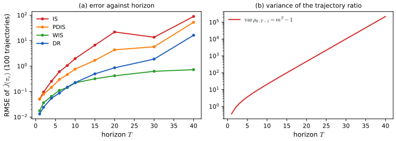
Demo: Off-policy value estimation: IS, PDIS, self-normalised IS and DR against the horizon.
35.5.3 The deadly triad
pp. 1176–1177, Figure 35.10, (35.59), (35.60) Off-policy data can also make a value-based method unstable or divergent. Baird's counterexample (1995; Figure 35.10(a)) has 7 states and 2 actions: the dashed action leads to one of the 6 upper states uniformly at random, the solid action to the bottom state; every reward is 0 and \(\gamma=0.99\). The value is linear, \(V_{\bm w}\) with \(\bm w\in\R^8\), with the expressions shown inside the states (\(2w_i+w_8\) for the upper state \(i\), \(w_7+2w_8\) for the bottom one). The target policy always takes the solid action, so \(V_\pi\equiv0\), representable with \(\bm w=0\). The behaviour policy takes dashed and solid with probabilities \(6/7\) and \(1/7\). TD(0) run on a trajectory of the behaviour policy diverges (Figure 35.10(b)), whereas with on-policy data linear TD(0) is guaranteed to converge to a good approximation (Tsitsiklis and Van Roy 1997). The divergence is seen with TD, Q-learning and related approximate dynamic-programming methods, for linear and for nonlinear representations (Gordon 1995, Bertsekas 2019). The root cause is that bootstrapping methods do not minimise a fixed objective: they build a target out of their own estimates, a self-reinforcing loop that can push the estimates to infinity. Formally, the contraction property (34.87) of the tabular case may fail once \(V\) is approximated by \(V_{\bm w}\). Any algorithm that combines off-policy learning, bootstrapping and function approximation may be unstable, the deadly triad (Sutton and Barto 2018); it is a subject of ongoing research. Gap 35.24 explains Baird's example by the eigenvalues of the expected update matrix.
Filling the gap 35.24: linear TD is stable on-policy; Baird's counterexample has an unstable eigenvalue pp. 1176–1177, Figure 35.10
Derivation
The mean dynamics. Consider semi-gradient TD(0) with a linear value \(V_{\bm w}=\Phi\bm w\), states drawn from a distribution \(d\) (\(D=\diag(d)\)), the next state from the target policy's transition matrix \(P_\pi\) (an importance ratio \(\rho=\pi/b\) makes the actions follow \(\pi\) in expectation), and zero rewards. The expected update is \[ \E[\rho\delta\bm\phi(s)]=\Phi^\T D(\gamma P_\pi\Phi\bm w-\Phi\bm w)=-A\bm w,\qquad A=\Phi^\T D(I-\gamma P_\pi)\Phi \] (with rewards, \(+\Phi^\T D\bm r_\pi\)). For a small step size the iterates follow \(\dot{\bm w}=-A\bm w\), which converges to 0 for every start iff all eigenvalues of \(A\) have positive real part, and diverges along an eigenvector with an eigenvalue of negative real part (the discrete iteration \(\bm w\leftarrow(I-\alpha A)\bm w\) has \(|1-\alpha\lambda|^2=1-2\alpha\operatorname{Re}\lambda+\alpha^2|\lambda|^2>1\) for small \(\alpha\) when \(\operatorname{Re}\lambda<0\)).
On-policy: \(A\) has a positive definite symmetric part. Let \(d\) be the stationary distribution of \(P=P_\pi\), \(d^\T P=d^\T\). For any \(v\), Jensen's inequality and stationarity give \(\|Pv\|_D^2=\sum_sd(s)\bigl(\sum_{s'}P(s'\given s)v(s')\bigr)^2\le\sum_sd(s)\sum_{s'}P(s'\given s)v(s')^2=\sum_{s'}d(s')v(s')^2=\|v\|_D^2\). So \(v^\T D(I-\gamma P)v=\|v\|_D^2-\gamma v^\T DPv\ge\|v\|_D^2-\gamma\|v\|_D\|Pv\|_D\ge(1-\gamma)\|v\|_D^2\) (Cauchy-Schwarz in the \(D\)-inner product). With \(v=\Phi\bm w\) and \(\Phi\) of full column rank, \(\bm w^\T A\bm w\ge(1-\gamma)\|\Phi\bm w\|_D^2>0\): the symmetric part of \(A\) is positive definite, so every eigenvalue has \(\operatorname{Re}\lambda=\operatorname{Re}(\bm z^\H A\bm z)/\|\bm z\|^2>0\), and the mean dynamics converge to the TD fixed point \(A^{-1}\bm b\) (Tsitsiklis and Van Roy 1997). Equivalently \(\Pi_DT_\pi\) is a \(\gamma\)-contraction in the \(D\)-norm for the on-policy distribution. A numerical experiment: for a random six-state chain with three random features the smallest eigenvalue of the symmetric part of \(A\) was positive. If instead \(D\) is not the stationary distribution of \(P_\pi\), \(\|Pv\|_D\) can exceed \(\|v\|_D\), the argument fails, and so may the contraction of the projected operator: this is the off-policy case.
Baird's example. The features are \(\phi(\text{upper }i)=2\bm e_i+\bm e_8\) and \(\phi(\text{lower})=\bm e_7+2\bm e_8\), the behaviour policy induces the uniform state distribution \(d=\tfrac17\) (each upper state has probability \(\tfrac67\cdot\tfrac16\), the bottom state \(\tfrac17\)), and under the target policy every state moves to the bottom state, \(P_\pi=\bm 1\bm e_7^\T\). The matrix \(A=\Phi^\T D(I-\gamma P_\pi)\Phi\) (an \(8\times8\) matrix of rank 7) has eigenvalue \(-0.2393\) (together with the eigenvalues \(-0.022\), 0 and others), so \(\bm w=0\) is unstable. In the simulation the expected update (step 0.01 from the book's start \(\bm w=(1,1,1,1,1,1,10,1)\)) reaches norm 437 after 1000 steps (\(w_8=335\)), and the sampled semi-gradient TD(0) on a trajectory of the behaviour policy with importance ratio 7 (solid) or 0 (dashed) also diverges (\(w_8=242\) after 1000 steps), as in the book's panel (b). If the behaviour policy is evaluated with its own data, the matrix has all eigenvalues with non-negative real part (smallest \(1.5\times10^{-18}\); the zero is the redundant direction of the 8 features for 7 states) and the weights stay bounded (norm 8.7).
Remedies. A convergent off-policy method needs an objective that does not move: minimising the squared Bellman error with the right correction for double sampling (gap 35.25), gradient-TD methods, or the distribution correction of Section 35.5.2; the book mentions path consistency learning and SBEED.
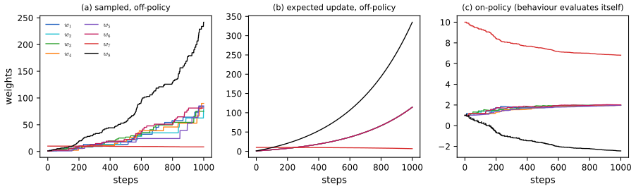
Demo: Baird's counterexample, with the behaviour probability, step size and discount adjustable.
p. 1177, (35.59), (35.60) A general way to ensure convergence off-policy is to minimise an objective whose minimum is a good value function. A natural candidate is the discrepancy of the two sides of the Bellman optimality equation (34.82), but the max is unfriendly to optimisation, so an entropy term smooths the greedy policy, which gives the squared loss of path consistency learning (PCL; Nachum et al. 2017), \[ \min_{V,\pi}\mathcal L_{\mathrm{PCL}}(V,\pi)\triangleq\E\Bigl[\tfrac12\bigl(r+\gamma V(s')-\lambda\log\pi(a\given s)-V(s)\bigr)^2\Bigr], \tag{35.59} \] over \((s,a,r,s')\) from some off-policy distribution (for example uniform over \(\D\)). Its minimiser is not the optimal value function and policy in general, because of the "double sampling" issue (Sutton and Barto 2018, Sec. 11.5). It is mitigated by a dual function (Dai et al. 2018), \[ \min_{V,\pi}\max_\nu\mathcal L_{\mathrm{SBEED}}(V,\pi;\nu)\triangleq\E\Bigl[\nu(s,a)\bigl(r+\gamma V(s')-\lambda\log\pi(a\given s)-V(s)\bigr)-\nu(s,a)^2/2\Bigr], \tag{35.60} \] with \(\nu\) in a function class (a network or an RKHS), which forces \(\nu\) to model the Bellman error, hence smoothed Bellman error embedding (SBEED). Both objectives can be minimised by gradient methods on parameterised \(V\) and \(\pi\). In the book's printed (35.60) the first term has the bracket squared; the form above (linear in the bracket) is the one that works, see gap 35.25.
Filling the gap 35.25: double sampling, why PCL is biased, and why SBEED needs the linear form p. 1177, (35.59), (35.60)
Derivation
The double-sampling bias. Let \(\delta=r+\gamma V(s')-\lambda\log\pi(a\given s)-V(s)\). For fixed \((s,a)\), \(\E[\delta^2\given s,a]=\bigl(\E[\delta\given s,a]\bigr)^2+\var(\delta\given s,a)=(\text{Bellman error})^2+\gamma^2\var(V(s')\given s,a)+\var(r\given s,a)\). Minimising the sampled squared TD error (35.59) therefore minimises the squared Bellman error plus a penalty on the variance of the value at the next state, which favours value functions that are smooth across the random successors rather than ones with zero Bellman error. To get an unbiased estimate of \((\E\delta)^2\) one needs two independent next-state samples from the same \((s,a)\) ("double sampling"), usually unavailable.
A numerical example. One state with value \(V=w\), feature 1; reward \(r=1\); the successor has feature 0.2 or 1.8 with probability \(\tfrac12\) each (so the mean feature is 1 and \(V(s')=0.2w\) or \(1.8w\)); \(\gamma=0.9\). The Bellman error is \(1+0.9w-w=1-0.1w\), zero at \(w=10\) (the true value: \(V=1+0.9V\)). The expected squared TD error is \((1-0.1w)^2+0.81\cdot0.64\,w^2\), minimised at \(w=0.189\): the minimiser of (35.59) is off by a factor 50, because the variance penalty \(\gamma^2\var(V(s'))\propto w^2\) pulls \(w\) toward 0 (I minimised both numerically).
SBEED. The Fenchel identity \(\tfrac12x^2=\max_\nu(\nu x-\tfrac12\nu^2)\), attained at \(\nu=x\), applied to \(x=\E[\delta\given s,a]\) gives \[ \tfrac12\bigl(\E[\delta\given s,a]\bigr)^2=\max_\nu\bigl\{\nu\,\E[\delta\given s,a]-\tfrac12\nu^2\bigr\}=\max_\nu\E\bigl[\nu\delta-\tfrac12\nu^2\given s,a\bigr], \] and since the maximisation is over a function \(\nu(s,a)\) that does not depend on \(s'\) (or on \(r\)), the expectation of the single-sample objective \(\nu\delta-\tfrac12\nu^2\) over \((r,s')\) equals \(\nu\,\E[\delta\given s,a]-\tfrac12\nu^2\) exactly: the sample version of (35.60) is unbiased for the squared Bellman error with no double sampling. The maximiser is \(\nu_*(s,a)=\E[\delta\given s,a]\), the Bellman error itself ("\(\nu\) models the Bellman error"), and \(\min_{V,\pi}\max_\nu\mathcal L_{\mathrm{SBEED}}=\min_{V,\pi}\tfrac12\E_{s,a}[(\E[\delta\given s,a])^2]\), the Bellman-error objective. In the example the inner maximum equals \(\tfrac12(1-0.1w)^2\), minimised at \(w=10\).
The printed formula. In (35.60) of the book the bracket \(\delta\) is squared. With \(\nu\delta^2-\nu^2/2\) the inner maximum is at \(\nu_*=\E[\delta^2\given s,a]\), with value \(\tfrac12(\E[\delta^2\given s,a])^2\): the second moment (which contains the variance term) again, not the Bellman error, and \(\nu\) would not model the Bellman error as the text says. In the example the minimiser of \(\tfrac12(\E\delta^2)^2\) is again \(w=0.189\). So the exponent in the printed formula is a typographical slip for the linear form of Dai et al. (2018).
35.5.4 Some common off-policy methods
p. 1177 Common online off-policy RL methods are Q-learning (Section 35.2.5), soft actor-critic (SAC, Section 35.6.1), DDPG and its relatives such as TD3 (Section 35.3.5), and MPO (maximum a posteriori policy optimisation; Abdolmaleki et al. 2018), a bound-optimisation method based on EM, the off-policy counterpart of the on-policy PPO of Section 35.3.4.
35.6 Control as inference
pp. 1177–1183 Another route to policy optimisation reduces it to probabilistic inference (Attias 2003, Toussaint and Storkey 2006, Toussaint 2009, Botvinick and Toussaint 2012, Kappen et al. 2012, Levine 2018). This lets one incorporate domain knowledge in the model and use the tools of approximate inference (Chapter 7) in a consistent framework.
35.6.1 Maximum entropy reinforcement learning
pp. 1178–1180, Figure 35.11, (35.61)–(35.73) Following Levine (2018), add to the MDP a binary variable \(o_t\) (Figure 35.11: \(o_t\) depends on \(s_t,a_t\); states and actions are observed, the optimality variables are not) that says whether the action at time \(t\) is optimal, with \[ p(o_t=1\given s_t,a_t)=\exp\bigl(\lambda^{-1}R(s_t,a_t)\bigr), \tag{35.61} \] for a temperature \(\lambda>0\) (this is a valid probability if \(R<0\), no loss of generality up to a constant; a non-informative uniform action prior \(p(a_t\given s_t)\) can be assumed, because any prior can be absorbed into (35.61)). The likelihood of a length-\(T\) trajectory when every step is optimal is \[ p(\tau\given o_{0:T-1}=1)\propto p(\tau,o_{0:T-1}=1)\propto p(s_0)\prod_{t=0}^{T-1}p(s_{t+1}\given s_t,a_t)\exp\Bigl(\frac1\lambda\sum_{t=0}^{T-1}R(s_t,a_t)\Bigr). \tag{35.62} \] With deterministic transitions this is proportional to \(\exp(\lambda^{-1}\sum_tR)\) for feasible trajectories and 0 otherwise, so maximising reward is the same as inferring the most probable trajectory. The posterior policy is \[ p(a_t\given s_t,o_{t:T-1}=1)\propto\frac{p(o_{t:T-1}=1\given s_t,a_t)}{p(o_{t:T-1}=1\given s_t)}, \tag{35.63} \] with, starting from \(p(o_{T-1}=1\given s_{T-1},a_{T-1})=\exp(\lambda^{-1}R(s_{T-1},a_{T-1}))\), the backward messages \[ p(o_{t:T-1}=1\given s_t,a_t)=\int_{\mathcal S}p(o_{t+1:T-1}=1\given s_{t+1})\,p(s_{t+1}\given s_t,a_t)\exp\bigl(\lambda^{-1}R(s_t,a_t)\bigr)\d s_{t+1}, \tag{35.64} \] \[ p(o_{t:T-1}=1\given s_t)=\int_{\mathcal A}p(o_{t:T-1}=1\given s_t,a_t)\,p(a_t\given s_t)\d a_t. \tag{35.65} \] This is expensive, so one approximates the optimal policy by a parametric \(\pi_{\bm\theta}\) with trajectory distribution \(p_{\bm\theta}(\tau)=p(s_1)\prod_tp(s_{t+1}\given s_t,a_t)\pi_{\bm\theta}(a_t\given s_t)\) (35.66) and minimises \(\KL(p_{\bm\theta}(\tau)\|p(\tau\given o_{0:T-1}=1))\), which simplifies to \[ \KL\bigl(p_{\bm\theta}(\tau)\,\|\,p(\tau\given o_{0:T-1}=1)\bigr)=-\E_{p_{\bm\theta}}\Bigl[\sum_{t=0}^{T-1}\lambda^{-1}R(s_t,a_t)+\Ent(\pi_{\bm\theta}(s_t))\Bigr]+\const. \tag{35.67} \] So the objective is to maximise reward with an entropy bonus favouring more uniform policies: maximum entropy RL (MERL). If \(\pi_{\bm\theta}\) can represent every stochastic policy, a softmax Bellman equation holds, \[ Q_*(s_t,a_t)=\lambda^{-1}R(s_t,a_t)+\E_{p(s_{t+1}\given s_t,a_t)}\Bigl[\log\int_{\mathcal A}\exp\bigl(Q_*(s_{t+1},a_{t+1})\bigr)\d a_{t+1}\Bigr], \tag{35.68} \] with \(Q_*(s_T,\cdot)=0\), and the optimal policy is \(\pi_*(a_t\given s_t)\propto\exp(Q_*(s_t,a_t))\). This \(Q_*\) differs from the usual one (34.83) because of the entropy, but as \(\lambda\to0\) the difference vanishes and the softmax policy becomes greedy. The soft actor-critic (SAC; Haarnoja et al. 2018) is an off-policy actor-critic method with the equivalent objective (\(T\to\infty\)) \[ J_{\mathrm{SAC}}(\bm\theta)\triangleq\E_{p^\infty_{\pi_{\bm\theta}}(s)\pi_{\bm\theta}(a\given s)}\bigl[R(s,a)+\lambda\Ent(\pi_{\bm\theta}(s))\bigr]. \tag{35.69} \] It works with soft value approximations \[ Q_{\bm w}(s,a)=R(s,a)+\gamma\E_{p(s'\given s,a)}\bigl[V_{\bm u}(s',a')-\lambda\log\pi_{\bm\theta}(a'\given s')\bigr],\qquad V_{\bm u}(s)=\lambda\log\sum_a\exp\bigl(\lambda^{-1}Q_{\bm w}(s,a)\bigr), \tag{35.70, 35.71} \] (printed with spurious arguments, see Notes on the book), which induce the improved policy \(\pi_{\bm w}(a\given s)=\exp(\lambda^{-1}Q_{\bm w}(s,a))/Z_{\bm w}(s)\); a soft policy-improvement step updates \(\bm\theta\) by minimising \(\E[\KL(\pi_{\bm\theta}(s)\|\pi_{\bm w}(s))]\) over states sampled from a replay buffer. SAC beats the off-policy DDPG and the on-policy PPO by a wide margin on continuous control (Haarnoja et al. 2018). A variant models only the action-value function, since both soft value and policy follow from it, \[ V_{\bm w}(s)=\lambda\log\sum_a\exp(\lambda^{-1}Q_{\bm w}(s,a)),\qquad\pi_{\bm w}(a\given s)=\exp\bigl(\lambda^{-1}(Q_{\bm w}(s,a)-V_{\bm w}(s))\bigr), \tag{35.72, 35.73} \] and is trained like DQN: soft Q-learning (Haarnoja et al. 2017), convenient with few actions or when the integral for \(V_{\bm w}\) is easy. It resembles PCL and SBEED of Section 35.5.3, which minimise objectives from the entropy-smoothed Bellman equation. Gap 35.26 derives (35.67) and (35.68), and shows that the exact messages (35.64, 35.65) give a different, optimistic recursion when the dynamics are stochastic.
Filling the gap 35.26: maximum-entropy RL from a KL divergence, the soft Bellman equation, and the optimism of exact inference pp. 1177–1180, (35.61)–(35.73)
Derivation
The KL objective (35.67). With the uniform action prior the target trajectory distribution is \(\tilde p(\tau)=p(s_0)\prod_tp(s_{t+1}\given s_t,a_t)\,e^{R_t/\lambda}/\tilde Z\) (the constant factor \(|\mathcal A|^{-T}\) of the prior is absorbed into \(\tilde Z\)). The approximating distribution (35.66) uses the true dynamics and only changes the policy. Hence the dynamics terms cancel in the log ratio: \[ \log\frac{p_{\bm\theta}(\tau)}{\tilde p(\tau)}=\sum_t\Bigl(\log\pi_{\bm\theta}(a_t\given s_t)-\frac{R_t}\lambda\Bigr)+\log\tilde Z, \] and taking the expectation under \(p_{\bm\theta}\), \(\E[\log\pi_{\bm\theta}(a_t\given s_t)]=-\E[\Ent(\pi_{\bm\theta}(s_t))]\), which gives (35.67). Minimising the KL is maximising \(\E[\sum_t\lambda^{-1}R_t+\Ent(\pi_{\bm\theta}(s_t))]\).
The soft Bellman equation (35.68). Define \(V_t(s)=\max_\pi\E[\sum_{k\ge t}(\lambda^{-1}R_k+\Ent(\pi(s_k)))\given s_t=s]\), \(V_T=0\), and \(Q_t(s,a)=\lambda^{-1}R(s,a)+\E_{s'}V_{t+1}(s')\). The Bellman principle gives \(V_t(s)=\max_{\pi(\cdot\given s)}\sum_a\pi(a\given s)(Q_t(s,a)-\log\pi(a\given s))\). The Gibbs variational principle evaluates this: for any distribution \(\pi\) and \(Z=\sum_ae^{Q(a)}\), \[ \sum_a\pi(a)\bigl(Q(a)-\log\pi(a)\bigr)=\log Z-\KL\Bigl(\pi\,\Big\|\,\frac{e^{Q}}{Z}\Bigr)\le\log Z, \] with equality iff \(\pi=\softmax(Q)\). So \(V_t(s)=\log\sum_ae^{Q_t(s,a)}\) and \(\pi_t(a\given s)\propto e^{Q_t(s,a)}\), which is (35.68) in finite-horizon form (the expectation over \(s'\) sits outside the log). For the discounted problem \(\E\sum_t\gamma^t(R_t+\lambda\Ent)\) the same argument with \(\lambda\) restored gives \(Q=R+\gamma\E V'\), \(V(s)=\lambda\log\sum_ae^{Q(s,a)/\lambda}\) and \(\pi=\exp((Q-V)/\lambda)\) (35.71 to 35.73); the policy is automatically normalised because of the definition of \(V\). Since \(\max_aQ\le\lambda\log\sum_ae^{Q/\lambda}\le\max_aQ+\lambda\log|\mathcal A|\), the soft value is within \(\lambda\log|\mathcal A|/(1-\gamma)\) of the standard optimal value, so the standard Bellman equation and the greedy policy are recovered as \(\lambda\to0\).
Exact inference is optimistic. The exact backward messages (35.64, 35.65) with the uniform prior are \(\beta_t(s,a)=e^{R(s,a)/\lambda}\,\E_{s'}[\beta_{t+1}(s')]\), \(\beta_t(s)=\frac1{|\mathcal A|}\sum_a\beta_t(s,a)\), and the posterior policy is \(\propto\beta_t(s,a)\). In logarithms, \(\log\beta_t(s,a)=R/\lambda+\log\E_{s'}\bigl[\exp(\log\beta_{t+1}(s'))\bigr]\), whereas the soft Bellman equation has \(R/\lambda+\E_{s'}[V_{t+1}(s')]\). By Jensen's inequality \(\log\E e^X\ge\E X\), with equality when \(s'\) is deterministic. So for stochastic dynamics the exact posterior values a next state by the log of an average of exponentials, dominated by the luckiest successor: it is optimistic about transitions (it infers the dynamics that would make the optimal trajectory likely, not those that exist), while the variational objective (35.66, 35.67) keeps the real dynamics and gives the realistic soft Bellman recursion (35.68). That is the reason for the restriction to \(\pi_{\bm\theta}\) in (35.66). In a three-state, two-action example with negative rewards and \(T=4\) I checked that the two recursions give the same policy for deterministic transitions (the two differ only by the constant \(\log|\mathcal A|\) per step, which does not affect a softmax) and different policies for random transitions.
Numerical experiments. On a random 4-state, 3-action MDP (\(\gamma=0.9\), \(\lambda=0.5\)) soft value iteration returned the policy that BFGS found by maximising \(J(\pi)+\lambda\E[\sum\gamma^t\Ent(\pi(s_t))]\) over the 12 softmax parameters (maximum difference \(2\times10^{-7}\), and the same optimal value); for \(\lambda=10^{-3}\) the soft-optimal policy attains the standard optimal return to 0.1%.
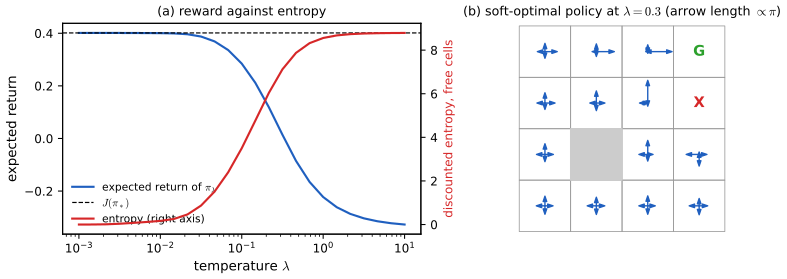
35.6.2 Other approaches
pp. 1180–1181, (35.74)–(35.78) VIREL (Fellows et al. 2019) is an alternative to maximum entropy RL. Like SAC it uses an approximate action-value function \(Q_{\bm w}\), a stochastic policy \(\pi_{\bm\theta}\) and a binary optimality variable, but with a different model, \[ p(o_t=1\given s_t,a_t)=\exp\Bigl(\frac{Q_{\bm w}(s_t,a_t)-\max_aQ_{\bm w}(s_t,a)}{\lambda_{\bm w}}\Bigr), \tag{35.74} \] whose temperature \(\lambda_{\bm w}\) is also parameterised and learned. An EM method maximises \(\mathcal L(\bm w,\bm\theta)=\E_{p(s)}\bigl[\E_{\pi_{\bm\theta}(a\given s)}[Q_{\bm w}(s,a)/\lambda_{\bm w}]+\Ent(\pi_{\bm\theta}(s))\bigr]\) (35.75) for a distribution \(p\) that is easy to sample from (a replay buffer): the E-step improves the actor, \(\bm\theta\leftarrow\bm\theta+\eta_\theta\nabla_{\bm\theta}\mathcal L\) (35.76), the M-step the critic, \(\bm w\leftarrow\bm w+\eta_w\nabla_{\bm w}\mathcal L\) (35.77). Other reductions of control to inference maximise the expected trajectory return \(J(\pi_{\bm\theta})=\int G(\tau)p(\tau\given\bm\theta)\d\tau\) (35.78) by treating \(G\) as a pseudo-likelihood (Peters and Schaal 2007, Neumann 2011, Abdolmaleki et al. 2018). Some have an objective like MERL's with the distribution containing \(\bm\theta\) in the second argument of the KL; the forward KL is mode-covering, which in RL is argued to be less desirable than the mode-seeking reverse KL of MERL (Section 2.7.1; Levine 2018).
Active inference is closely related and rests on the free-energy principle of neuroscience (Friston 2009 and others). With hidden states \(s\), observations \(y\) and parameters \(\theta\), the variational free energy is \(F[p,q](y)=\KL(q(s,\theta\given y)\|p(s,\theta\given y))-\log p(y)\); state estimation (perception) minimises \(F\) over \(q(s\given y,\theta)\) and parameter estimation (learning) over \(q(\theta\given y)\), as in variational Bayes EM (Chapter 10). If \(p(s,y\given\theta)\) is a nonlinear hierarchical Gaussian model and \(q(s\given y,\theta)=\N(s\given\hat s,H)\) a Laplace approximation (mode found by gradient descent, \(H\) the Hessian at the mode), one recovers predictive coding, a non-amortised VAE (Chapter 21) with inference and learning both by gradient descent (a more efficient incremental-EM version updates all \(\hat s_n\) and \(\theta\) in parallel, Salvatori et al. 2024). For decisions, the expected free energy \(F(\bm a)=\E_{q(y\given\bm a)}[F(y)]\) is defined for an action sequence \(\bm a\) through the posterior predictive \(q(y\given\bm a)\), the policy is \(\pi(\bm a)=\softmax(F(\bm a))\), and the prior \(p(s)\propto e^{R(s)}\) (or over observations \(p(y)\propto e^{R(y)}\)) encodes the preferred outcomes: the generative model describes what the agent wants rather than an objective model of the world, which induces goal-directed information seeking, unlike the goal-independent uncertainty of the maximum-entropy approach. Despite this, the technique is very similar to control as inference (Millidge et al. 2020 and others). I do not develop it further.
35.6.3 Imitation learning
p. 1182 In imitation learning (IL; also apprenticeship learning or learning from demonstration) the agent sees no rewards, only a set \(\D_{\exp}\) of trajectories \(\tau=(s_0,a_0,s_1,a_1,\dots,s_T)\) generated by an expert policy, \(a_t\sim\pi_{\exp}(s_t)\), and must learn a good policy by imitating it. Typical uses are driving and dialogue, where writing a reward is hard (survey: Osa et al. 2018).
35.6.3.1 Imitation learning by behavior cloning
p. 1182, (35.79) Behaviour cloning (Pomerleau 1989) treats the policy as a classifier from states to actions, minimising an imitation error such as \[ \min_\pi\E_{p^\infty_{\pi_{\exp}}(s)}\bigl[\KL(\pi_{\exp}(s)\,\|\,\pi(s))\bigr], \tag{35.79} \] approximating the expectation by an average over the states of \(\D_{\exp}\). The loss ignores the sequential structure: a policy \(\hat\pi\) that is accurate on the expert's state distribution may still be badly wrong on its own state distribution \(p^\infty_{\hat\pi}\) when run, because its mistakes lead to states the expert never visited. More demonstrations or algorithmic additions handle the mismatch (Daume et al. 2009, Ross et al. 2011). Gap 35.27 quantifies the mismatch.
Filling the gap 35.27: behaviour cloning errors compound quadratically in the horizon p. 1182, (35.79)
Derivation
The bound. Let \(\hat\pi\) satisfy \(\E_{s_t\sim p_t^{\exp}}[\TV(\hat\pi(s_t),\pi_{\exp}(s_t))]\le\varepsilon\) for every \(t<T\) (the expected total variation error measured on the expert's own state distribution; by Pinsker this is implied by a small KL (35.79)). Run two agents, the expert and the clone, with the following coupling: while their histories agree, draw their actions by a maximal coupling of \(\pi_{\exp}(s_t)\) and \(\hat\pi(s_t)\), which disagree with probability \(\TV_t(s_t)\); the next states are drawn identically, so the histories stay equal until the first disagreement. The probability that the first disagreement occurs at step \(t\) is \(\E[\ind[\text{histories agree up to }t]\TV_t(s_t)]\le\E_{s_t\sim p_t^{\exp}}[\TV_t(s_t)]\le\varepsilon\), because on the event that the histories agree, \(s_t\) is distributed as the expert's state (restricted to a sub-probability). A union bound over the \(T\) steps gives \(\Pr(\text{histories differ})\le\varepsilon T\), hence the total variation distance between the trajectory distributions is at most \(\varepsilon T\), and since the return lies in \([0,TR_{\max}]\), \[ J(\pi_{\exp})-J(\hat\pi)\le TR_{\max}\cdot\varepsilon T=R_{\max}\varepsilon T^2. \] The error grows quadratically in the horizon although the supervised error per step is \(\varepsilon\).
The bound is attained up to a constant. Take a "tightrope": in the good states the expert's action gives reward 1; any other action sends the agent to an absorbing state with reward 0 for ever, and the clone picks a wrong action with probability \(\varepsilon\) at each good state. The clone's expected reward at step \(t\) is \((1-\varepsilon)^t\), so the shortfall over \(T\) steps is \(T-\sum_{t<T}(1-\varepsilon)^t=\sum_{t<T}(1-(1-\varepsilon)^t)\le\varepsilon T(T-1)/2\), with equality up to higher-order terms of \(\varepsilon T\): about \(\varepsilon T^2/2\). Numerically, \(\varepsilon=0.02\), \(T=40\): the shortfall is 12.3 against the bound \(\varepsilon T(T-1)/2=15.6\); for \(\varepsilon=0.001\) it is within 2% of \(\varepsilon T(T-1)/2\). The remedies cited in the book (interactive expert queries, as in DAgger) reduce the dependence to linear in \(T\) by training on the states the clone itself visits.
35.6.3.2 Imitation learning by inverse reinforcement learning
pp. 1182–1183, (35.80), (35.81) Inverse RL (IRL, or inverse optimal control; Ng and Russell 2000) first infers a reward function that explains the expert trajectories and then computes a (near-)optimal policy for it with any RL algorithm. Infinitely many rewards make the expert optimal (for example by the optimality-preserving transformations of Ng et al. 1999), so the maximum-entropy principle (Section 2.4.7) is used with an energy-based model of the expert (Ziebart et al. 2008), \[ p(\tau)\propto\exp\Bigl(\sum_{t=0}^{T-1}R_{\bm\theta}(s_t,a_t)\Bigr)=\exp(R_{\bm\theta}(\tau)), \tag{35.80} \] which gives exponentially small probability to trajectories of low cumulative reward. The partition function \(Z_{\bm\theta}=\int e^{R_{\bm\theta}(\tau)}\d\tau\) is intractable and must be approximated, here by sampling: let \(\D_{\exp}\) and \(\D\) be trajectories from the expert and from a known distribution \(q\); then the negative log-likelihood is \[ \mathcal L(\bm\theta)=-\frac1{|\D_{\exp}|}\sum_{\tau\in\D_{\exp}}R_{\bm\theta}(\tau)+\log\frac1{|\D|}\sum_{\tau\in\D}\frac{\exp(R_{\bm\theta}(\tau))}{q(\tau)}. \tag{35.81} \] The term in the log is an importance-sampling estimate of \(Z_{\bm\theta}\), unbiased if \(q>0\) wherever needed. To reduce the variance \(q\) is adapted as \(\bm\theta\) changes: the optimal sampler \(q_*(\tau)\propto\exp(R_{\bm\theta}(\tau))\) (Section 11.5) is not available, but a policy \(\hat\pi\) that induces a distribution close to it can be found by maximum-entropy RL (Section 35.6.1), which yields both the reward and an approximately optimal policy: guided cost learning (Finn et al. 2016), effective in robotics. Gap 35.28 proves the likelihood gradient, the partition-function estimate and the reward-shaping invariance.
Filling the gap 35.28: the gradient of the maximum-entropy IRL likelihood, the unbiased estimate of Z, and reward shaping pp. 1182–1183, (35.80), (35.81)
Derivation
The gradient. With \(p_{\bm\theta}(\tau)=e^{R_{\bm\theta}(\tau)}/Z_{\bm\theta}\), the per-trajectory negative log-likelihood is \(-R_{\bm\theta}(\tau)+\log Z_{\bm\theta}\) and \(\nabla_{\bm\theta}\log Z_{\bm\theta}=\frac1{Z_{\bm\theta}}\int e^{R_{\bm\theta}(\tau)}\nabla R_{\bm\theta}(\tau)\d\tau=\E_{p_{\bm\theta}}[\nabla R_{\bm\theta}(\tau)]\). Hence \[ \nabla_{\bm\theta}\mathcal L=-\E_{\D_{\exp}}[\nabla R_{\bm\theta}(\tau)]+\E_{p_{\bm\theta}}[\nabla R_{\bm\theta}(\tau)]. \] For a linear reward \(R_{\bm\theta}(\tau)=\bm\theta^\T\bm\phi(\tau)\) (\(\bm\phi\) feature counts) the loss is convex (log-sum-exp is convex) and at the optimum the model's expected feature counts equal the expert's, \(\E_{p_{\bm\theta}}[\bm\phi]=\E_{\D_{\exp}}[\bm\phi]\): the reward is learned so that the model reproduces the demonstrations' statistics. On the 8 trajectories of a 3-state, 2-action deterministic MDP with \(T=3\) I verified the gradient formula against finite differences (to \(10^{-6}\)) and that BFGS reaches a point where the feature expectations match to \(10^{-4}\).
The partition function. If \(q(\tau)>0\) wherever \(e^{R_{\bm\theta}(\tau)}>0\), then \(\E_{\tau\sim q}[e^{R_{\bm\theta}(\tau)}/q(\tau)]=\int e^{R_{\bm\theta}(\tau)}\d\tau=Z_{\bm\theta}\): the average inside the log of (35.81) is unbiased for \(Z_{\bm\theta}\). The loss itself uses \(\log\hat Z\), and by Jensen's inequality \(\E\log\hat Z\le\log Z\), so with a finite sample the estimated loss is biased downwards, with a bias that shrinks as the sample grows and the proposal approaches \(q_*\) (for which \(e^R/q\) is constant and the variance is zero). I checked unbiasedness of \(\hat Z\) by simulation (200,000 uniform proposals over the 8 trajectories).
Reward shaping. For any function \(\Phi(s)\), the reward \(R'(s,a)=R(s,a)+\gamma\E_{s'}[\Phi(s')]-\Phi(s)\) has \(Q'_\pi(s,a)=Q_\pi(s,a)-\Phi(s)\) for every policy \(\pi\): the extra terms telescope along any trajectory, \(\sum_t\gamma^t(\gamma\Phi(s_{t+1})-\Phi(s_t))=-\Phi(s_0)+\lim\gamma^T\Phi(s_T)\). Since the shift is the same for all actions at a state, \(R\) and \(R'\) have the same greedy and optimal policies, so the expert's behaviour cannot identify the reward beyond such transformations; the maximum-entropy principle selects one member of the family.
35.6.3.3 Imitation learning by divergence minimization
p. 1183, (35.82) The reward depends only on the state and action, so if \(p^\infty_\pi(s,a)\) and \(p^\infty_{\pi_{\exp}}(s,a)\) are close then \(\pi\) earns about the same long-term reward as the expert. Many IL algorithms minimise a divergence between the two occupancy measures (Ghasemipour et al. 2019, Ke et al. 2019). With a convex \(f\) and the variational form of \(D_f\) (Nguyen et al. 2010) one solves \[ \min_\pi\max_{\bm w}\ \E_{p^\infty_{\pi_{\exp}}(s,a)}[T_{\bm w}(s,a)]-\E_{p^\infty_\pi(s,a)}[f^*(T_{\bm w}(s,a))], \tag{35.82} \] with \(T_{\bm w}:\mathcal S\times\mathcal A\to\R\) a parametrised function and \(f^*\) the convex conjugate of \(f\). The first expectation is estimated from \(\D_{\exp}\) as in behaviour cloning, the second from trajectories of \(\pi\); a parametric \(\pi_{\bm\theta}\) and stochastic gradient steps seek a saddle point. Different \(f\) give generative adversarial imitation learning (GAIL; Ho and Ermon 2016), adversarial inverse RL (AIRL; Fu et al. 2018) and new methods such as \(f\)-MAX and forward adversarial inverse RL (FAIRL; Ghasemipour et al. 2019, Ke et al. 2019). Running \(\pi\) to estimate the second expectation may be costly or risky, in which case one is in the off-policy IL setting and uses the corrections of Section 35.5 (ValueDICE, Kostrikov et al. 2020, uses the distribution correction of DualDICE). Gap 35.29 proves the variational form.
Filling the gap 35.29: the variational form of the f-divergence behind (35.82) p. 1183, (35.82)
Derivation
The identity. Let \(f\) be convex and lower semicontinuous, \(D_f(p\|q)=\E_q[f(p/q)]\), and \(f^*(t)=\sup_u(tu-f(u))\) its conjugate. By the Fenchel-Moreau theorem \(f(u)=\sup_t(tu-f^*(t))\). Apply this pointwise with \(u=p(x)/q(x)\) and multiply by \(q(x)\): \[ q(x)f\Bigl(\frac{p(x)}{q(x)}\Bigr)=\sup_t\bigl(t\,p(x)-q(x)f^*(t)\bigr). \] Integrating over \(x\), the supremum over functions \(T(x)\) is attained pointwise, so \[ D_f(p\|q)=\sup_T\ \E_p[T(x)]-\E_q[f^*(T(x))],\qquad T_*(x)=f'\bigl(p(x)/q(x)\bigr), \] the maximiser being the pointwise maximiser \(t=f'(u)\) of \(tu-f^*(t)\) (since \(u\in\partial f^*(t)\) iff \(t\in\partial f(u)\)). Restricting \(T\) to a parametric class \(T_{\bm w}\) gives a lower bound \(\E_p[T_{\bm w}]-\E_q[f^*(T_{\bm w})]\le D_f(p\|q)\), tight if the class contains \(T_*\). In (35.82) \(p=p^\infty_{\pi_{\exp}}\) and \(q=p^\infty_\pi\), so the saddle-point problem minimises \(D_f(p^\infty_{\pi_{\exp}}\|p^\infty_\pi)\) over \(\pi\) (the game of Section 26.2.3 with the roles of data and model, here expert and policy).
Which KL. With \(f(u)=u\log u\), \(D_f(p_{\exp}\|p_\pi)=\KL(p_{\exp}\|p_\pi)\), the forward (mode-covering) KL, and \(f^*(t)=e^{t-1}\); with \(f(u)=-\log u\) one gets the reverse (mode-seeking) \(\KL(p_\pi\|p_{\exp})\), \(f^*(t)=-1-\log(-t)\) for \(t<0\); with \(f(u)=(u-1)^2\), the Pearson \(\chi^2\) divergence with \(f^*(t)=t^2/4+t\). I verified numerically for random distributions on five points that \(\E_p[T_*]-\E_q[f^*(T_*)]\) equals \(D_f(p\|q)\) to \(10^{-9}\) for these three choices and that 2000 random perturbations of \(T_*\) never exceeded it.
Supplement S35
The supplement chapter S35, titled "Reinforcement learning" (pages 309 and 310 of the supplement), consists of a title page and a blank page in this draft; there is no content to cover. Everything on reinforcement learning is in Sections 35.1 to 35.6 of the main text.
Demonstrations
Practice problems
The book has no exercises for this chapter. These three short problems are my own.
Practice problem 35.1 (a lambda-return by hand). An episode has three steps with rewards \(r_0,r_1,r_2=0,0,1\), \(\gamma=0.9\), and current value estimates \(V(s_0),V(s_1),V(s_2)=0.5,0.4,0.3\) (the terminal value is 0). Compute the \(n\)-step returns \(G_{0:1},G_{0:2},G_{0:3}\), the \(\lambda\)-return \(G^\lambda_0\) for \(\lambda=0,\tfrac12,1\), and check the identity of gap 35.8 for \(\lambda=\tfrac12\).
Solution
\(G_{0:1}=0+0.9\cdot0.4=0.36\); \(G_{0:2}=0+0.9\cdot0+0.81\cdot0.3=0.243\); \(G_{0:3}=0.81\cdot1=0.81\) (the Monte Carlo return). With the weights \((1-\lambda),(1-\lambda)\lambda,\lambda^2\) on the three returns (the last weight absorbs the tail, as in gap 35.8): \(\lambda=0\) gives 0.36 (the TD(0) target), \(\lambda=1\) gives 0.81 (Monte Carlo), and \(\lambda=\tfrac12\): \(G^{1/2}_0=0.5\cdot0.36+0.25\cdot0.243+0.25\cdot0.81=0.18+0.06075+0.2025=0.44325\). TD errors: \(\delta_0=0+0.9\cdot0.4-0.5=-0.14\), \(\delta_1=0+0.9\cdot0.3-0.4=-0.13\), \(\delta_2=1+0-0.3=0.7\). Then \(\sum_\ell(\gamma\lambda)^\ell\delta_\ell=-0.14+0.45(-0.13)+0.2025(0.7)=-0.14-0.0585+0.14175=-0.05675=G^{1/2}_0-V(s_0)=0.44325-0.5\). The advantage estimate moves from \(-0.14\) (\(\lambda=0\)) to \(+0.31\) (\(\lambda=1\)): the bootstrapped estimate trusts the (poor) critic, the Monte Carlo one the observed reward.
Practice problem 35.2 (how many trajectories?). A target policy takes action 0 with probability 0.8 and action 1 with probability 0.2 in every state; the behaviour policy is uniform. (a) Compute \(m=\E_b[\rho^2]\) and the variance of the trajectory weight \(\prod_{t<T}\rho_t\) for \(T=20\). (b) The effective sample size of \(n\) importance-weighted trajectories is about \(n/\E[(\prod\rho)^2]\). How many trajectories give an effective sample size of 100 at \(T=20\)?
Solution
(a) \(\rho=1.6\) with probability \(\tfrac12\) and \(0.4\) with probability \(\tfrac12\), so \(\E\rho=1\) and \(m=\tfrac12(2.56+0.16)=1.36\) (equivalently \(\sum_a\pi_e^2/\pi_b=(0.64+0.04)/0.5\)). By independence \(\E[\prod\rho_t^2]=m^T\) and the variance of the weight is \(m^T-1=1.36^{20}-1=467.6\) (standard deviation 21.6). (b) \(n/m^{20}=100\) gives \(n=100\cdot468.57\approx4.7\times10^4\) trajectories; at \(T=40\) one would need \(100\cdot1.36^{40}\approx2.2\times10^7\). With the same policies a per-decision estimator needs fewer for the early rewards but the same order for the late ones; this exponential cost is the curse of horizon.
Practice problem 35.3 (a soft policy). A state has two actions with action values \(Q=(1,0)\). For temperatures \(\lambda=1\) and \(\lambda=\tfrac12\) compute the soft-optimal policy \(\pi_\lambda\), its entropy, and the soft value \(V=\lambda\log\sum_ae^{Q_a/\lambda}\); verify \(V=\E_\pi[Q]+\lambda\Ent(\pi)\) and find the limit \(\lambda\to0\).
Solution
\(\pi_\lambda(a_1)=\sigma(1/\lambda)\). For \(\lambda=1\): \(\pi=0.7311\), entropy \(-0.7311\ln0.7311-0.2689\ln0.2689=0.5822\), \(V=\log(e+1)=1.3133\), and \(\E_\pi[Q]+\lambda\Ent=0.7311+0.5822=1.3133\). For \(\lambda=\tfrac12\): \(\pi=\sigma(2)=0.8808\), entropy 0.3653, \(V=0.5\log(e^2+1)=1.0635=0.8808+0.5\cdot0.3653\). The identity is the Gibbs variational principle of gap 35.26 (\(V=\E_\pi[Q-\lambda\log\pi]\) for \(\pi=\softmax(Q/\lambda)\)). As \(\lambda\to0\), \(\pi\to(1,0)\), the entropy tends to 0 and \(V\to\max Q=1\), within \(\lambda\log2\) of it (\(V-1\le0.693\lambda\)): the standard greedy value is recovered.
Notes on the book
Slips and sharpenings found while proving and checking the claims
- Section 35.1.5.2, Table 35.2. In the fourth row (\(\hat R=5.05,4.95\)) the Boltzmann entries should be 0.52 and 0.48 (0.525 and 0.475); the printed 0.53 and 0.48 sum to 1.01. All other entries reproduce. Gap 35.2.
- Section 35.3.3.1. The one-sample advantage is written \(r_{t+1}+\gamma V_{\bm w}(s_{t+1})-V_{\bm w}(s_t)\); with the indexing of this chapter (\(r_t\) follows \(a_t\), (35.27)) it is \(r_t+\gamma V_{\bm w}(s_{t+1})-V_{\bm w}(s_t)\).
- Section 35.3.4, (35.34). The trust-region lower bound is printed with the coefficient \(\epsilon\gamma/(1-\gamma)^2\) on the maximum KL. The proof I can give (total variation coupling and Pinsker's inequality, gap 35.14) yields \(2\epsilon\gamma/(1-\gamma)^2\) with \(\epsilon=\max_{s,a}|A_\pi|\). I do not claim the printed constant is false (a search for a counterexample found none), only that it is not what the standard argument gives.
- Section 35.3.4, (35.37). The PPO objective is stated as the clipped ratio times the advantage; the objective of the original paper is the minimum of the unclipped and clipped terms. They differ when \(A>0,\ r<1-\epsilon\) or \(A<0,\ r>1+\epsilon\), where the clip-only version has zero gradient (gap 35.15).
- Section 35.3.5, (35.40). \(\nabla_{\bm\theta}\mu_{\bm\theta}(s)\) is called an \(M\times N\) matrix (\(M\) the action dimension, \(N\) the number of parameters), but its product with the \(M\)-vector \(\nabla_aQ\) is an \(N\)-vector only if it is the \(N\times M\) matrix (the transposed Jacobian). (35.42) also has a stray \(\d s\) inside the expectation.
- Figure 35.10 caption. "Parameters of the policy diverge over time": the diverging parameters are those of the value function \(V_{\bm w}\) (the target policy has no parameters).
- Section 35.5.3, (35.60). The first term of the SBEED objective is printed with the bracket squared, \(\nu(\cdot)^2\); it should be linear, \(\nu(s,a)(r+\gamma V(s')-\lambda\log\pi(a\given s)-V(s))-\nu(s,a)^2/2\), for \(\nu\) to model the Bellman error and for the double-sampling bias to disappear (gap 35.25).
- Section 35.6.1, (35.70) and (35.71). \(V_{\bm u}(s',a')\) in (35.70) and \(V_{\bm u}(s,a)\) in (35.71) carry spurious action arguments: the soft value is a function of the state, \(V_{\bm u}(s')\) (or the sampled bracket \(Q(s',a')-\lambda\log\pi(a'\given s')\)) and \(V_{\bm u}(s)\).
- Section 35.6.1, from (35.64) to (35.68). The soft Bellman equation (35.68) follows from the variational objective (35.66, 35.67), not from the exact messages (35.64, 35.65), which for stochastic dynamics give \(\log\E_{s'}e^{V(s')}\) instead of \(\E_{s'}V(s')\) and are optimistic (gap 35.26). The two agree only for deterministic transitions.
References
- Murphy, K. P. (2023). Probabilistic Machine Learning: Advanced Topics. MIT Press, Cambridge, MA. Chapter 35, pp. 1145–1183. probml.github.io/pml-book/book2.html.
- Abdolmaleki, A. et al. (2018). Maximum a posteriori policy optimisation. International Conference on Learning Representations.
- Amos, B. and Yarats, D. (2020). The differentiable cross-entropy method. International Conference on Machine Learning.
- Auer, P., Cesa-Bianchi, N. and Fischer, P. (2002). Finite-time analysis of the multiarmed bandit problem. Machine Learning, 47, 235–256.
- Baird, L. (1995). Residual algorithms: reinforcement learning with function approximation. International Conference on Machine Learning.
- Bang, H. and Robins, J. M. (2005). Doubly robust estimation in missing data and causal inference models. Biometrics, 61, 962–973.
- Barto, A. G., Sutton, R. S. and Anderson, C. W. (1983). Neuronlike adaptive elements that can solve difficult learning control problems. IEEE Transactions on Systems, Man and Cybernetics, 13, 834–846.
- Bellemare, M. G., Dabney, W. and Munos, R. (2017). A distributional perspective on reinforcement learning. International Conference on Machine Learning.
- Bellemare, M. G. et al. (2016). Unifying count-based exploration and intrinsic motivation. Advances in Neural Information Processing Systems, 29.
- Bertsekas, D. P. (2019). Reinforcement Learning and Optimal Control. Athena Scientific.
- Chua, K., Calandra, R., McAllister, R. and Levine, S. (2018). Deep reinforcement learning in a handful of trials using probabilistic dynamics models. Advances in Neural Information Processing Systems, 31.
- Dai, B. et al. (2018). SBEED: convergent reinforcement learning with nonlinear function approximation. International Conference on Machine Learning.
- Degris, T., White, M. and Sutton, R. S. (2012). Off-policy actor-critic. International Conference on Machine Learning.
- Deisenroth, M. P. and Rasmussen, C. E. (2011). PILCO: a model-based and data-efficient approach to policy search. International Conference on Machine Learning.
- Ernst, D., Geurts, P. and Wehenkel, L. (2005). Tree-based batch mode reinforcement learning. Journal of Machine Learning Research, 6, 503–556.
- Finn, C., Levine, S. and Abbeel, P. (2016). Guided cost learning: deep inverse optimal control via policy optimization. International Conference on Machine Learning.
- Fortunato, M. et al. (2018). Noisy networks for exploration. International Conference on Learning Representations.
- Fu, J., Luo, K. and Levine, S. (2018). Learning robust rewards with adversarial inverse reinforcement learning. International Conference on Learning Representations.
- Fujimoto, S., van Hoof, H. and Meger, D. (2018). Addressing function approximation error in actor-critic methods. International Conference on Machine Learning.
- Gal, Y., McAllister, R. and Rasmussen, C. E. (2016). Improving PILCO with Bayesian neural network dynamics models. Data-Efficient Machine Learning workshop, ICML.
- Ghasemipour, S. K. S., Zemel, R. and Gu, S. (2019). A divergence minimization perspective on imitation learning methods. Conference on Robot Learning.
- Gordon, G. J. (1995). Stable function approximation in dynamic programming. International Conference on Machine Learning.
- Guez, A., Silver, D. and Dayan, P. (2013). Scalable and efficient Bayes-adaptive reinforcement learning based on Monte-Carlo tree search. Journal of Artificial Intelligence Research, 48, 841–883.
- Ha, D. and Schmidhuber, J. (2018). World models. arXiv:1803.10122.
- Haarnoja, T., Zhou, A., Abbeel, P. and Levine, S. (2018). Soft actor-critic: off-policy maximum entropy deep reinforcement learning with a stochastic actor. International Conference on Machine Learning.
- Hafner, D. et al. (2019). Learning latent dynamics for planning from pixels. International Conference on Machine Learning. Hafner, D. et al. (2020). Dream to control: learning behaviors by latent imagination. International Conference on Learning Representations.
- van Hasselt, H. (2010). Double Q-learning. Advances in Neural Information Processing Systems, 23. van Hasselt, H., Guez, A. and Silver, D. (2016). Deep reinforcement learning with double Q-learning. AAAI. van Hasselt, H. et al. (2016). Learning values across many orders of magnitude. Advances in Neural Information Processing Systems, 29.
- Hessel, M. et al. (2018). Rainbow: combining improvements in deep reinforcement learning. AAAI.
- Ho, J. and Ermon, S. (2016). Generative adversarial imitation learning. Advances in Neural Information Processing Systems, 29.
- Huang, J. and Jiang, N. (2020). From importance sampling to doubly robust policy gradient. International Conference on Machine Learning.
- Jaakkola, T., Jordan, M. I. and Singh, S. P. (1994). On the convergence of stochastic iterative dynamic programming algorithms. Neural Computation, 6, 1185–1201.
- Jacobson, D. H. and Mayne, D. Q. (1970). Differential Dynamic Programming. Elsevier.
- Janner, M., Fu, J., Zhang, M. and Levine, S. (2019). When to trust your model: model-based policy optimization. Advances in Neural Information Processing Systems, 32.
- Jiang, N. and Li, L. (2016). Doubly robust off-policy value evaluation for reinforcement learning. International Conference on Machine Learning.
- Kakade, S. and Langford, J. (2002). Approximately optimal approximate reinforcement learning. International Conference on Machine Learning.
- Kamthe, S. and Deisenroth, M. P. (2018). Data-efficient reinforcement learning with probabilistic model predictive control. Artificial Intelligence and Statistics.
- Kocsis, L. and Szepesvari, C. (2006). Bandit based Monte-Carlo planning. European Conference on Machine Learning.
- Kolter, J. Z. and Ng, A. Y. (2009). Near-Bayesian exploration in polynomial time. International Conference on Machine Learning.
- Levine, S. (2018). Reinforcement learning and control as probabilistic inference: tutorial and review. arXiv:1805.00909. Levine, S. et al. (2020). Offline reinforcement learning: tutorial, review, and perspectives on open problems. arXiv:2005.01643.
- Lillicrap, T. P. et al. (2016). Continuous control with deep reinforcement learning. International Conference on Learning Representations.
- Lin, L.-J. (1992). Self-improving reactive agents based on reinforcement learning, planning and teaching. Machine Learning, 8, 293–321.
- Liu, Q., Li, L., Tang, Z. and Zhou, D. (2018). Breaking the curse of horizon: infinite-horizon off-policy estimation. Advances in Neural Information Processing Systems, 31.
- Mania, H., Guy, A. and Recht, B. (2018). Simple random search provides a competitive approach to reinforcement learning. Advances in Neural Information Processing Systems, 31.
- Mnih, V. et al. (2015). Human-level control through deep reinforcement learning. Nature, 518, 529–533. Mnih, V. et al. (2016). Asynchronous methods for deep reinforcement learning. International Conference on Machine Learning.
- Munos, R., Stepleton, T., Harutyunyan, A. and Bellemare, M. G. (2016). Safe and efficient off-policy reinforcement learning. Advances in Neural Information Processing Systems, 29.
- Nachum, O. et al. (2017). Bridging the gap between value and policy based reinforcement learning. Advances in Neural Information Processing Systems, 30. Nachum, O., Chow, Y., Dai, B. and Li, L. (2019). DualDICE: behavior-agnostic estimation of discounted stationary distribution corrections. Advances in Neural Information Processing Systems, 32.
- Ng, A. Y., Harada, D. and Russell, S. (1999). Policy invariance under reward transformations: theory and application to reward shaping. International Conference on Machine Learning. Ng, A. Y. and Jordan, M. I. (2000). PEGASUS: a policy search method for large MDPs and POMDPs. Uncertainty in Artificial Intelligence.
- Nguyen, X., Wainwright, M. J. and Jordan, M. I. (2010). Estimating divergence functionals and the likelihood ratio by convex risk minimization. IEEE Transactions on Information Theory, 56, 5847–5861.
- Pirotta, M., Restelli, M., Pecorino, A. and Calandriello, D. (2013). Safe policy iteration. International Conference on Machine Learning.
- Precup, D., Sutton, R. S. and Singh, S. (2000). Eligibility traces for off-policy policy evaluation. International Conference on Machine Learning.
- Robbins, H. and Siegmund, D. (1971). A convergence theorem for non negative almost supermartingales and some applications. In Optimizing Methods in Statistics, Academic Press.
- Ross, S. and Bagnell, J. A. (2010). Efficient reductions for imitation learning. Artificial Intelligence and Statistics. Ross, S., Gordon, G. and Bagnell, J. A. (2011). A reduction of imitation learning and structured prediction to no-regret online learning. Artificial Intelligence and Statistics.
- Russo, D. J., Van Roy, B., Kazerouni, A., Osband, I. and Wen, Z. (2018). A tutorial on Thompson sampling. Foundations and Trends in Machine Learning, 11, 1–96.
- Salimans, T., Ho, J., Chen, X., Sidor, S. and Sutskever, I. (2017). Evolution strategies as a scalable alternative to reinforcement learning. arXiv:1703.03864.
- Schaul, T., Quan, J., Antonoglou, I. and Silver, D. (2016). Prioritized experience replay. International Conference on Learning Representations.
- Schulman, J. et al. (2015). Trust region policy optimization. International Conference on Machine Learning. Schulman, J. et al. (2016). High-dimensional continuous control using generalized advantage estimation. International Conference on Learning Representations. Schulman, J. et al. (2017). Proximal policy optimization algorithms. arXiv:1707.06347.
- Silver, D. et al. (2014). Deterministic policy gradient algorithms. International Conference on Machine Learning.
- Singh, S., Jaakkola, T., Littman, M. L. and Szepesvari, C. (2000). Convergence results for single-step on-policy reinforcement-learning algorithms. Machine Learning, 38, 287–308.
- Smith, J. E. and Winkler, R. L. (2006). The optimizer's curse: skepticism and postdecision surprise in decision analysis. Management Science, 52, 311–322.
- Strehl, A. L. and Littman, M. L. (2008). An analysis of model-based interval estimation for Markov decision processes. Journal of Computer and System Sciences, 74, 1309–1331.
- Sutton, R. S. (1988). Learning to predict by the methods of temporal differences. Machine Learning, 3, 9–44. Sutton, R. S. (1990). Integrated architectures for learning, planning, and reacting based on approximating dynamic programming. International Conference on Machine Learning. Sutton, R. S., McAllester, D., Singh, S. and Mansour, Y. (1999). Policy gradient methods for reinforcement learning with function approximation. Advances in Neural Information Processing Systems, 12.
- Sutton, R. S. and Barto, A. G. (2018). Reinforcement Learning: An Introduction, 2nd edition. MIT Press.
- Thomas, P. and Brunskill, E. (2016). Data-efficient off-policy policy evaluation for reinforcement learning. International Conference on Machine Learning.
- Tsitsiklis, J. N. (1994). Asynchronous stochastic approximation and Q-learning. Machine Learning, 16, 185–202. Tsitsiklis, J. N. and Van Roy, B. (1997). An analysis of temporal-difference learning with function approximation. IEEE Transactions on Automatic Control, 42, 674–690.
- Wang, Z. et al. (2016). Dueling network architectures for deep reinforcement learning. International Conference on Machine Learning.
- Williams, R. J. (1992). Simple statistical gradient-following algorithms for connectionist reinforcement learning. Machine Learning, 8, 229–256.
- Ziebart, B. D., Maas, A., Bagnell, J. A. and Dey, A. K. (2008). Maximum entropy inverse reinforcement learning. AAAI.
- Zintgraf, L. et al. (2020). VariBAD: a very good method for Bayes-adaptive deep RL via meta-learning. International Conference on Learning Representations.
The numerical statements in the text (Table 35.2, the Bellman-error identity, optimism of the count-based bonus, the Bayes-adaptive dynamic programme and its comparison with Thompson sampling and plug-in planning, the epsilon-soft optimum, convergence of synchronous Q-learning and GLIE SARSA, batch TD against batch Monte Carlo, the lambda-return identities and the n-step bias, the maximisation bias and Figure 35.5, fitted Q-iteration, the policy gradient theorem and the unbiasedness and variance of REINFORCE with baselines, the performance-difference lemma and the conservative and trust-region bounds, the natural-gradient step and the PPO clip, the deterministic policy gradient, the model predictive control bound, A*, the Riccati recursion and certainty equivalence, the Gaussian moments of a GP prediction, common random numbers, the unbiasedness of importance sampling, per-decision and doubly robust estimators, the stationary-ratio saddle point, Baird's counterexample, the double-sampling bias, soft value iteration and exact control as inference, the inverse-RL gradient, behaviour cloning and the f-divergence bound, and the practice problems) were confirmed numerically.