Introduction
Almost every idea of the book appears in miniature in this chapter. A polynomial is fitted to noisy data and over-fits; probability theory explains why, turns least squares into maximum likelihood and regularisation into a prior, and leads to a fully Bayesian prediction; decision theory says what to do with the probabilities; information theory supplies the entropy and the Kullback-Leibler divergence that run through the rest of the course.
Ch. 1 Introduction Ch. 2 Probability distributions Ch. 3 Linear regression Ch. 4 Linear classification Ch. 5 Neural networks Ch. 6 Kernel methods Ch. 7 Sparse kernel machines Ch. 8 Graphical models Ch. 9 Mixture models and EM Ch. 10 Approximate inference Ch. 11 Sampling methods Ch. 12 Continuous latent variables Ch. 13 Sequential data Ch. 14 Combining models
How to read these notes
They follow the book. Sections carry Bishop's numbers (1.1, 1.2.4, ...) and every displayed equation that appears in the book carries the book's own equation number, e.g. (1.62), so you can read these notes next to the book. Equations without a number are steps that the book skips.
Filling the gaps. Wherever the book says that a result "is easily shown", follows "after some manipulation", or is left as an exercise, an orange Filling the gap box or a proof gives the full argument. Proofs and derivations start hidden: open one with its bar, or use the button below.
Figures and demonstrations. The numerical figures of the chapter are reproduced from scratch by the Python code. The ▶ Demo boxes open an interactive demonstration already set to the case being discussed. Standard identities (Jensen's inequality, Lagrange multipliers, the calculus of variations, completing the square, Gaussian facts) are proved once in the mathematical toolkit and linked from here.
Main reference
C. M. Bishop, Pattern Recognition and Machine Learning, Springer (2006), Chapter 1, pages 1–58 (exercises on pages 58–66). Section, equation, figure and exercise numbers below refer to this book. Further reading is listed in the references.
The explanations, derivations and code are my own; equations are cited by their numbers in the book.
The chapter at a glance
- 1.1 Fitting \(y(x,\mathbf{w})=\sum_{j=0}^{M}w_jx^j\) by least squares is a linear problem with a closed-form solution (Result 1.1). The order \(M\) controls flexibility: \(M=9\) on \(N=10\) points interpolates the noise (over-fitting), and a quadratic penalty (ridge regression, Result 1.2) tames it.
- 1.2 The sum and product rules give Bayes' theorem. For the Gaussian, maximum likelihood underestimates the variance by the factor \((N-1)/N\) (Result 1.8). Seen probabilistically, least squares is maximum likelihood with Gaussian noise, and ridge regression is MAP estimation with \(\lambda=\alpha/\beta\); the full Bayesian predictive distribution adds the parameter uncertainty to the noise (Result 1.11).
- 1.3, 1.4 Cross-validation, AIC and BIC choose model complexity; in high dimensions volume and probability mass sit in thin shells (Results 1.13 and 1.14).
- 1.5 Decision theory: assign each \(\mathbf{x}\) to the class of largest posterior to minimise the error rate, or minimise \(\sum_kL_{kj}\,p(\mathcal{C}_k\given\mathbf{x})\) for a loss matrix; add a reject option; for regression the squared loss gives the conditional mean, absolute loss the median.
- 1.6 Entropy is maximal for the uniform distribution (discrete) and the Gaussian (fixed variance); the KL divergence is non-negative by Jensen's inequality, and the mutual information is the KL divergence from independence.
Notation. Training inputs \(\mathbf{x}=(x_1,\dots,x_N)^\T\) and targets \(\mathbf{t}=(t_1,\dots,t_N)^\T\); \(\mathbf{w}\) the coefficients; \(\bm{\phi}(x)=(1,x,\dots,x^M)^\T\) so that \(y(x,\mathbf{w})=\mathbf{w}^\T\bm{\phi}(x)\); \(\bm{\Phi}\) the \(N\times(M+1)\) design matrix with rows \(\bm{\phi}(x_n)^\T\); precision \(\beta=1/\sigma^2\). The book uses a sans-serif x for the data set of scalar inputs; here the data set is also written \(\mathbf{x}\), and the individual points are \(x_n\).
Prerequisites. Only calculus, linear algebra and elementary probability. The chapter is self-contained; later chapters are cross-referenced where the book looks forward.
Printings. The text used here is a corrected printing. Where Bishop's errata list corrects an equation or exercise of this chapter ((1.72), (1.90), (1.100), (1.103), (1.119), Exercises 1.16, 1.20, 1.32, 1.34 and the caption of Figure 1.27), the notes give the corrected form and a short Erratum note.
What this chapter does
pp. 1–5 Pattern recognition is the automatic discovery of regularities in data and their use to act: assigning a handwritten digit (Figure 1.1) to one of ten classes, predicting a real-valued target, grouping similar items, or reducing dimension. The book distinguishes supervised learning (training examples come with target values: classification if the target is a discrete class label, regression if it is continuous), unsupervised learning (no targets: clustering, density estimation, visualisation) and reinforcement learning (find actions that maximise a reward, with a trade-off between exploration and exploitation). A learned function is judged by its generalisation, its performance on new inputs, not by its fit to the training set. Raw inputs are usually transformed first (feature extraction, pre-processing): this can make the problem easier, and must be applied identically to the test data.
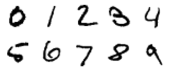
fig1_1. Download: PDF · SVGThree threads are tied together in this chapter and are followed by the rest of the course: probability theory to describe uncertainty, decision theory to turn probabilities into actions, and information theory to measure how well one distribution approximates another. The running example, polynomial curve fitting, is used to meet each of them in a concrete setting.
1.1 Example: polynomial curve fitting
pp. 4–12 The data are generated as follows (the book, p. 4): take \(x_n\) equally spaced in \([0,1]\), compute \(\sin(2\pi x_n)\), and add Gaussian noise of standard deviation \(0.3\) to get \(t_n\). The training set has \(N=10\) points (Figure 1.2); a test set of 100 further points is generated the same way. The aim is to predict \(t\) for a new \(x\), without knowing the sine. Fit the polynomial
\[ y(x,\mathbf{w})=w_0+w_1x+w_2x^2+\dots+w_Mx^M=\sum_{j=0}^{M}w_jx^j, \tag{1.1} \]which is nonlinear in \(x\) but linear in the coefficients \(\mathbf{w}\); this is what makes everything below closed-form. The coefficients minimise the sum-of-squares error
\[ E(\mathbf{w})=\frac12\sum_{n=1}^{N}\{y(x_n,\mathbf{w})-t_n\}^2, \tag{1.2} \]half the sum of the squared vertical displacements of Figure 1.3.
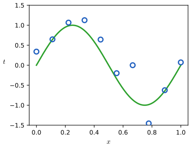
fig1_2. Download: PDF · SVG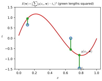
fig1_3. Download: PDF · SVGResult 1.1 (the normal equations; Exercise 1.1) p. 6, (1.122), (1.123)
The sum-of-squares error (1.2) with the polynomial (1.1) is a convex quadratic in \(\mathbf{w}\). Its stationary points are exactly the solutions of the linear system
\[ \sum_{j=0}^{M}A_{ij}w_j=T_i,\quad i=0,\dots,M,\qquad A_{ij}=\sum_{n=1}^{N}(x_n)^{i+j},\quad T_i=\sum_{n=1}^{N}(x_n)^{i}t_n, \tag{1.122, 1.123} \]that is \(\bm{\Phi}^\T\bm{\Phi}\,\mathbf{w}\)
Proof
The equations. Differentiate (1.2) with respect to \(w_i\), using \(\partial y(x_n,\mathbf{w})/\partial w_i\)
Setting this to zero for \(i=0,\dots,M\) is (1.122). In matrix form \(\Phi_{nj}=x_n^{\,j}\), \(\mathbf{A}=\bm{\Phi}^\T\bm{\Phi}\), \(\mathbf{T}=\bm{\Phi}^\T\mathbf{t}\), and \(E(\mathbf{w})\)
Minimum, and uniqueness. For any \(\mathbf{v}\), \(E(\mathbf{w}+\mathbf{v})\)
Interpolation. If \(N=M+1\) the Vandermonde matrix \(\bm{\Phi}\) is square with \(\det\bm{\Phi}=\prod_{m\lt n}(x_n-x_m)\neq0\), so \(\bm{\Phi}\mathbf{w}=\mathbf{t}\) has a solution and \(E(\mathbf{w}^\star)=0\). This is the situation of \(M=9\), \(N=10\) in Figure 1.4.∎
The remaining question is the order \(M\), an example of model selection. Figure 1.4 shows \(M=0,1,3,9\): the constant and the line under-fit, the cubic is close to the sine, and the ninth-order polynomial passes through every point (\(E(\mathbf{w}^\star)=0\)) but oscillates wildly between them. This is over-fitting.
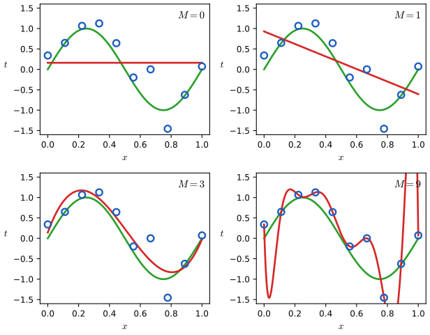
fig1_4. Download: PDF · SVGDefinition 1.1 (root-mean-square error) p. 7, (1.3)
For a fitted \(\mathbf{w}^\star\) on a data set of \(N\) points, \(E_{\mathrm{RMS}}=\sqrt{2E(\mathbf{w}^\star)/N}\). Since \(2E=\sum_n\{y(x_n,\mathbf{w}^\star)-t_n\}^2\), this is the square root of the mean squared residual: division by \(N\) puts data sets of different sizes on an equal footing, and the square root returns the units of \(t\).
\[ E_{\mathrm{RMS}}=\sqrt{2E(\mathbf{w}^\star)/N}. \tag{1.3} \]Figure 1.5 plots \(E_{\mathrm{RMS}}\) on the training set and on a 100-point test set against \(M\). The training error decreases monotonically (a polynomial of order \(M\) contains all those of lower order, so the minimum over a larger set cannot increase) and reaches zero at \(M=9\). The test error is high for small \(M\) (too inflexible), small for \(3\le M\le 8\), and explodes at \(M=9\).
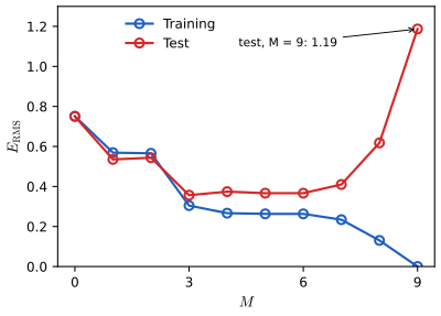
fig1_5. Download: PDF · SVGFilling the gap 1.1: why the coefficients explode and why more data helps pp. 8–9, Table 1.1, Figure 1.6
The book observes that the coefficients \(\mathbf{w}^\star\) grow to the order of \(10^5\) for \(M=9\) (its Table 1.1) and that over-fitting weakens as \(N\) grows (Figure 1.6), but only intuitively.
Derivation
Large coefficients. At \(M=9\), \(N=10\), the solution is \(\mathbf{w}^\star=\bm{\Phi}^{-1}\mathbf{t}\) with \(\bm{\Phi}\) a Vandermonde matrix. The monomials \(1,x,\dots,x^9\) on \([0,1]\) are nearly linearly dependent (the matrix \(\bm{\Phi}\) is very ill conditioned), so a vector \(\mathbf{v}\) with tiny \(\|\bm{\Phi}\mathbf{v}\|\) but large \(\|\mathbf{v}\|\) exists: the smallest singular value \(s_{\min}\) of \(\bm{\Phi}\) is small. Writing \(\bm{\Phi}=\sum_is_i\mathbf{u}_i\mathbf{v}_i^\T\) (SVD),
\[ \mathbf{w}^\star=\sum_i\frac{\mathbf{u}_i^\T\mathbf{t}}{s_i}\,\mathbf{v}_i . \]The component of the noise \(\bm{\varepsilon}=\mathbf{t}-\sin(2\pi\mathbf{x})\) along \(\mathbf{u}_{\min}\) is amplified by \(1/s_{\min}\) in \(\mathbf{w}^\star\) and the large coefficients cancel each other at the data points but not between them. The coefficients are "finely tuned to the noise".
More data. With \(N\gg M+1\) the system is over-determined: \(\mathbf{w}^\star\) averages the noise over many points. Formally, if the noise is independent with variance \(\sigma^2\), \(\mathrm{cov}[\mathbf{w}^\star]\)
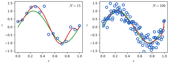
fig1_6. Download: PDF · SVGA heuristic is that the number of points should be a multiple (5 or 10) of the number of parameters, but it is unsatisfying to let the amount of data fix the model's complexity; the Bayesian treatment of Section 1.2.6 has no such restriction. Meanwhile, a standard remedy is regularisation: add a penalty on the size of the coefficients,
\[ \widetilde E(\mathbf{w})=\frac12\sum_{n=1}^{N}\{y(x_n,\mathbf{w})-t_n\}^2+\frac{\lambda}{2}\|\mathbf{w}\|^2,\qquad \|\mathbf{w}\|^2=\mathbf{w}^\T\mathbf{w}=w_0^2+\dots+w_M^2 . \tag{1.4} \]The particular case of a quadratic penalty is ridge regression (Hoerl and Kennard, 1970; see Hastie et al., 2009) in statistics and weight decay in neural networks; such methods are called shrinkage methods. The intercept \(w_0\) is often left out of the penalty (so that the fit does not depend on the origin of \(t\)); the derivation below covers both choices.
Result 1.2 (ridge regression; Exercise 1.2) p. 10, (1.4)
The regularised error (1.4) has the unique minimiser, for every \(\lambda>0\) and every data set,
\[ \sum_{j=0}^{M}(A_{ij}+\lambda\,\delta_{ij})\,w_j=T_i,\qquad \mathbf{w}^\star_\lambda=(\bm{\Phi}^\T\bm{\Phi}+\lambda\mathbf{I})^{-1}\bm{\Phi}^\T\mathbf{t}. \]With the SVD \(\bm{\Phi}=\sum_is_i\mathbf{u}_i\mathbf{v}_i^\T\), \(\mathbf{w}^\star_\lambda\)
Proof
The gradient of (1.4) is \(\partial\widetilde E/\partial w_i\)
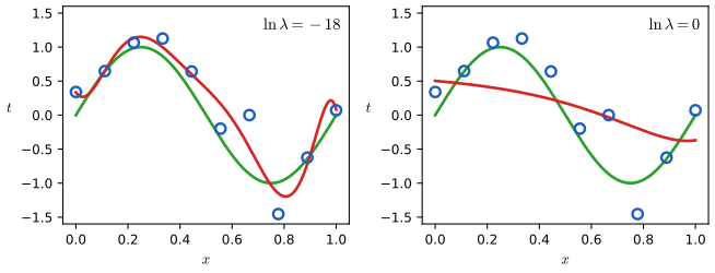
fig1_7. Download: PDF · SVG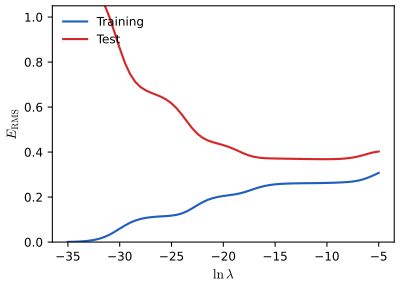
fig1_8. Download: PDF · SVGSo \(\lambda\) now plays the role of \(M\): it fixes the effective complexity of the model. To choose it (or \(M\)) we can split the data into a training set (to find \(\mathbf{w}\)) and a validation or hold-out set (to optimise \(M\) or \(\lambda\)); Section 1.3 discusses the wasteful side of this and how cross-validation reduces it.
1.2 Probability theory
pp. 12–17 Uncertainty enters pattern recognition through noise on measurements and through the finiteness of the data. Probability theory is the consistent calculus for it. The book's example: a red box holds 2 apples and 6 oranges, a blue box 3 apples and 1 orange (Figure 1.9); a box is picked (red with probability \(4/10\), blue with \(6/10\)), then a fruit is drawn uniformly from it. \(B\in\{r,b\}\) is the box and \(F\in\{a,o\}\) the fruit.
To derive the rules, count. In \(N\) trials let \(n_{ij}\) be the number with \(X=x_i\) and \(Y=y_j\), \(c_i=\sum_jn_{ij}\) the number with \(X=x_i\) (a column of Figure 1.10) and \(r_j\) the number with \(Y=y_j\). In the limit \(N\to\infty\) the joint and marginal probabilities are
\[ p(X=x_i,Y=y_j)=\frac{n_{ij}}{N},\qquad\text{(1.5)}\qquad p(X=x_i)=\frac{c_i}{N}.\tag{1.6} \]Because \(c_i=\sum_jn_{ij}\), dividing by \(N\) gives the sum rule \(p(X=x_i)=\sum_{j=1}^{L}p(X=x_i,Y=y_j)\) (1.7). The conditional probability of \(Y=y_j\) among the instances with \(X=x_i\) is \(p(Y=y_j\given X=x_i)=n_{ij}/c_i\) (1.8), and then
\[ p(X=x_i,Y=y_j)=\frac{n_{ij}}{N}=\frac{n_{ij}}{c_i}\cdot\frac{c_i}{N}=p(Y=y_j\given X=x_i)\,p(X=x_i), \tag{1.9} \]the product rule. In the compact notation:
Definition 1.2 (rules of probability, Bayes' theorem) pp. 14–15, (1.10)–(1.13)
\[ \text{sum rule: }\ p(X)=\sum_Yp(X,Y), \tag{1.10} \] \[ \text{product rule: }\ p(X,Y)=p(Y\given X)\,p(X). \tag{1.11} \]Using the symmetry \(p(X,Y)=p(Y,X)\) and the product rule twice gives Bayes' theorem, and the sum rule expresses the denominator through the numerator:
\[ p(Y\given X)=\frac{p(X\given Y)\,p(Y)}{p(X)},\qquad\text{(1.12)}\qquad p(X)=\sum_Yp(X\given Y)\,p(Y). \tag{1.13} \]The denominator is the normalising constant that makes \(\sum_Yp(Y\given X)=1\). \(X\) and \(Y\) are independent if \(p(X,Y)=p(X)p(Y)\), equivalently \(p(Y\given X)=p(Y)\).
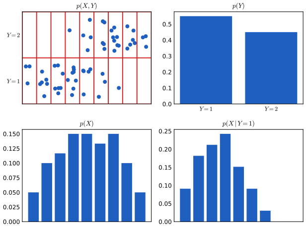
fig1_11. Download: PDF · SVGWorked example: the boxes of fruit pp. 15–17, (1.14)–(1.23)
Priors \(p(B=r)=4/10\), \(p(B=b)=6/10\) (1.14, 1.15); conditionals \(p(F=a\given r)=1/4\), \(p(F=o\given r)=3/4\), \(p(F=a\given b)=3/4\), \(p(F=o\given b)=1/4\) (1.16)–(1.19). By the sum and product rules
\[ p(F=a)=p(a\given r)p(r)+p(a\given b)p(b)=\tfrac14\cdot\tfrac4{10}+\tfrac34\cdot\tfrac6{10}=\tfrac{11}{20},\qquad p(F=o)=\tfrac9{20}. \tag{1.22} \]If the fruit is an orange, Bayes' theorem gives the posterior of the box:
\[ p(B=r\given F=o)=\frac{p(o\given r)\,p(r)}{p(o)}=\frac34\cdot\frac4{10}\cdot\frac{20}{9}=\frac23,\qquad p(B=b\given F=o)=\frac13. \tag{1.23} \]Before seeing the fruit the blue box was more likely (\(6/10\)); the orange is so much more probable under the red box that the posterior reverses this. \(p(B)\) is the prior, \(p(B\given F)\) the posterior. (The fruit is not independent of the box, since \(p(F\given B)\) depends on \(B\); it would be independent only if both boxes had the same fraction of apples.)
1.2.1 Probability densities
pp. 17–19 For a continuous variable, \(p(x)\) is a density: the probability of \((x,x+\delta x)\) is \(p(x)\delta x\) as \(\delta x\to0\), so that
\[ p(x\in(a,b))=\int_a^bp(x)\,\d x,\qquad p(x)\ge0,\ \ \int_{-\infty}^{\infty}p(x)\,\d x=1 , \tag{1.24, 1.25, 1.26} \]and the cumulative distribution function is \(P(z)=\int_{-\infty}^zp(x)\d x\) (1.28), with \(P'(x)=p(x)\). In several dimensions \(p(\mathbf{x})\ge0\), \(\int p(\mathbf{x})\d\mathbf{x}=1\) (1.29, 1.30). The sum and product rules and Bayes' theorem hold unchanged, with sums replaced by integrals:
\[ p(x)=\int p(x,y)\,\d y,\qquad\text{(1.31)}\qquad p(x,y)=p(y\given x)\,p(x). \tag{1.32} \]Under a change of variable \(x=g(y)\), a density transforms with the Jacobian, unlike an ordinary function \(\widetilde f(y)=f(g(y))\):
\[ p_y(y)=p_x(x)\left|\frac{\d x}{\d y}\right|=p_x(g(y))\,|g'(y)|. \tag{1.27} \]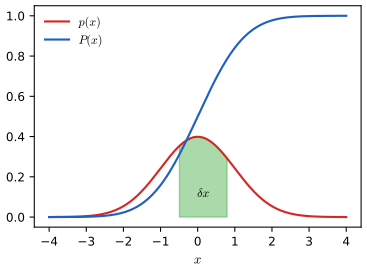
fig1_12. Download: PDF · SVGFilling the gap 1.2: the Jacobian factor, and why the mode depends on the variable (Exercise 1.4) p. 18, (1.27)
The book states that the maximum of a density depends on the choice of variable. Here is why, and when it does not.
Derivation
Why (1.27). Let \(g\) be a differentiable, strictly monotone map. The events \(\{x\in(x,x+\delta x)\}\) and \(\{y\in(y,y+\delta y)\}\) with \(x=g(y)\) and \(\delta x\approx g'(y)\delta y\) are the same event, so \(p_x(x)|\delta x|\simeq p_y(y)|\delta y|\), i.e. \(p_y(y)=p_x(g(y))|g'(y)|\). (Equivalently, for increasing \(g\), \(P_y(y)=P_x(g(y))\); differentiate. For decreasing \(g\) the sign flips and the absolute value appears.)
The modes. Let \(\hat x\) maximise \(p_x\), so \(p_x'(\hat x)=0\), and let \(\hat y=g^{-1}(\hat x)\). Take \(g'>0\) for simplicity. Differentiating (1.27) with the chain rule,
\[ p_y'(y)=p_x'(g(y))\,g'(y)^2+p_x(g(y))\,g''(y). \]At \(y=\hat y\) the first term vanishes and \(p_y'(\hat y)=p_x(\hat x)\,g''(\hat y)\), which is not zero unless \(g''(\hat y)=0\) (note \(p_x(\hat x)>0\)). So \(\hat y\) is in general not a stationary point of \(p_y\): the maximum of \(p_y\) is at a different \(y\), and \(\hat x\ne g(\hat y_{\rm mode})\). The Jacobian \(|g'(y)|\) multiplies the density and shifts its peak. If \(g\) is linear, \(g(y)=ay+b\) with \(a\neq0\), then \(g''=0\) and \(g'^2=a^2>0\): \(p_y'(y)=a^2p_x'(ay+b)\) vanishes exactly where \(p_x'\) does, so \(\hat x=g(\hat y)\), and the location of the maximum transforms like the variable itself.
Example. Let \(x\sim\mathcal{N}(0,1)\) and \(x=g(y)=\ln y\) (\(y>0\)). Then \(p_y(y)=\mathcal{N}(\ln y\given0,1)/y\), the log-normal density. Setting the derivative of \(\ln p_y=-\tfrac12(\ln y)^2-\ln y+\mathrm{const}\) to zero gives \(-(\ln y+1)/y=0\), so the mode is \(y=\mathrm{e}^{-1}\), whereas the image of the mode of \(x\) is \(g^{-1}(0)=1\).∎
1.2.2 Expectations and covariances
pp. 19–20 The average of a function \(f\) under \(p\) is the expectation
\[ \E[f]=\sum_xp(x)f(x),\qquad\text{(1.33)}\qquad \E[f]=\int p(x)f(x)\,\d x. \tag{1.34} \]Given \(N\) samples \(x_n\) from \(p\), \(\E[f]\simeq\frac1N\sum_nf(x_n)\) (1.35), exact as \(N\to\infty\) (Chapter 11). With several variables a subscript names the averaged one: \(\E_x[f(x,y)]\) (1.36) is a function of \(y\); the conditional expectation is \(\E_x[f\given y]=\sum_xp(x\given y)f(x)\) (1.37). The variance and the covariance are
\[ \var[f]=\E\big[(f(x)-\E[f(x)])^2\big],\qquad\text{(1.38)}\qquad \cov[x,y]=\E_{x,y}\big[\{x-\E[x]\}\{y-\E[y]\}\big]=\E_{x,y}[xy]-\E[x]\E[y] , \tag{1.41} \]and for vectors \(\cov[\mathbf{x},\mathbf{y}]\)
Result 1.3 (variance and covariance identities; Exercises 1.5, 1.6, 1.10) pp. 20, 59, (1.39)–(1.41), (1.128), (1.129)
(a) \(\var[f]=\E[f(x)^2]-\E[f(x)]^2\), in particular \(\var[x]=\E[x^2]-\E[x]^2\). (b) \(\E_{x,y}[\{x-\E x\}\{y-\E y\}]=\E[xy]-\E[x]\E[y]\). (c) If \(x\) and \(y\) are independent, \(\cov[x,y]=0\). (d) If \(x\) and \(z\) are independent, \(\E[x+z]=\E[x]+\E[z]\) and \(\var[x+z]=\var[x]+\var[z]\). (The mean formula needs no independence.)
Proof
(a) Write \(\mu=\E[f]\), a constant. Expanding the square and using linearity of \(\E\): \(\E[(f-\mu)^2]\)
The converse of (c) is false: uncorrelated variables need not be independent (take \(x\sim\mathcal{N}(0,1)\), \(y=x^2\): \(\cov[x,y]=\E x^3=0\) yet \(y\) is a function of \(x\)).
1.2.3 Bayesian probabilities
pp. 21–23 So far probability was a long-run frequency of repeatable events. It is also a degree of belief about uncertain, possibly unrepeatable, events (will this polar ice cap melt by 2100?); Cox and Jaynes showed that the sum and product rules are the unique consistent calculus for such degrees of belief. For curve fitting we want to say something about \(\mathbf{w}\) itself. Before seeing the data we express our assumptions as a prior \(p(\mathbf{w})\); the data \(\mathcal{D}=\{t_1,\dots,t_N\}\) enter through the likelihood \(p(\mathcal{D}\given\mathbf{w})\) and Bayes' theorem gives the posterior
\[ p(\mathbf{w}\given\mathcal{D})=\frac{p(\mathcal{D}\given\mathbf{w})\,p(\mathbf{w})}{p(\mathcal{D})},\qquad\text{(1.43)}\qquad \text{posterior}\ \propto\ \text{likelihood}\times\text{prior}, \tag{1.44} \]where the denominator is the normaliser, found by integrating the numerator over \(\mathbf{w}\) (the sum rule):
\[ p(\mathcal{D})=\int p(\mathcal{D}\given\mathbf{w})\,p(\mathbf{w})\,\d\mathbf{w}. \tag{1.45} \]The likelihood \(p(\mathcal{D}\given\mathbf{w})\) is a function of \(\mathbf{w}\) for fixed data. In a frequentist treatment \(\mathbf{w}\) is a fixed parameter estimated by, e.g., maximum likelihood, and its uncertainty is assessed by the distribution of the estimator over imagined data sets (the bootstrap: resample the data with replacement to create many data sets). In a Bayesian treatment there is one observed data set and the uncertainty is the distribution of \(\mathbf{w}\) given it. Advantages: prior knowledge enters naturally, and extreme data are handled gracefully (a coin that shows three heads in three tosses should not be given probability 1 of heads: maximum likelihood does, a prior does not). The price is the dependence on the prior, which is sometimes chosen for convenience (conjugate priors, Chapter 2), and the computational cost of the integrals, now reduced by sampling (Chapter 11) and deterministic approximations (Chapter 10).
1.2.4 The Gaussian distribution
pp. 24–28 For a real variable \(x\), the Gaussian or normal distribution with mean \(\mu\) and variance \(\sigma^2\) (precision \(\beta=1/\sigma^2\)) is
\[ \mathcal{N}(x\given\mu,\sigma^2)=\frac{1}{(2\pi\sigma^2)^{1/2}}\exp\Big\{-\frac{1}{2\sigma^2}(x-\mu)^2\Big\}, \tag{1.46} \]which is positive, \(\mathcal{N}(x\given\mu,\sigma^2)>0\) (1.47), and normalised, symmetric about \(\mu\), with the properties
\[ \int_{-\infty}^{\infty}\mathcal{N}(x\given\mu,\sigma^2)\,\d x=1,\qquad\text{(1.48)}\qquad \E[x]=\mu,\qquad\text{(1.49)}\qquad \E[x^2]=\mu^2+\sigma^2,\qquad\text{(1.50)}\qquad \var[x]=\sigma^2. \tag{1.51} \]The maximum of the density is the mode; for the Gaussian it equals the mean (Exercise 1.9). In \(D\) dimensions
\[ \mathcal{N}(\mathbf{x}\given\bm\mu,\bm\Sigma)=\frac{1}{(2\pi)^{D/2}}\frac{1}{|\bm\Sigma|^{1/2}}\exp\Big\{-\frac12(\mathbf{x}-\bm\mu)^\T\bm\Sigma^{-1}(\mathbf{x}-\bm\mu)\Big\}, \tag{1.52} \]with mean vector \(\bm\mu\) and covariance matrix \(\bm\Sigma\) (studied in Chapter 2).
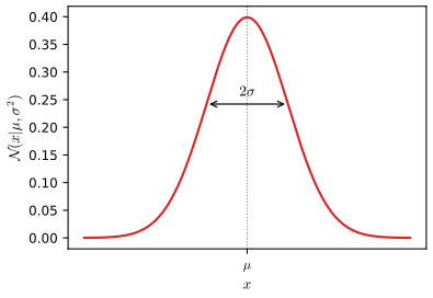
fig1_13. Download: PDF · SVGResult 1.4 (the Gaussian is normalised; Exercise 1.7) pp. 24, 59, (1.48), (1.124)–(1.126)
\(I\)
Proof (polar coordinates)
The integral \(I\) is finite and positive. Its square is a double integral over the plane (Fubini, the integrand is positive):
\[ I^2=\int_{-\infty}^{\infty}\!\!\int_{-\infty}^{\infty}\exp\Big(-\frac{1}{2\sigma^2}x^2-\frac{1}{2\sigma^2}y^2\Big)\d x\,\d y. \tag{1.125} \]Change to polar coordinates \(x=r\cos\theta\), \(y=r\sin\theta\) with \(\d x\,\d y=r\,\d r\,\d\theta\), \(r\in[0,\infty)\), \(\theta\in[0,2\pi)\); the integrand depends on \(r\) only:
\[ I^2=\int_0^{2\pi}\!\!\d\theta\int_0^{\infty}\exp\Big(-\frac{r^2}{2\sigma^2}\Big)r\,\d r=2\pi\cdot\frac12\int_0^{\infty}\exp\Big(-\frac{u}{2\sigma^2}\Big)\d u=\pi\cdot2\sigma^2=2\pi\sigma^2, \]with \(u=r^2\), \(\d u=2r\,\d r\), and \(\int_0^\infty\mathrm{e}^{-u/2\sigma^2}\d u\)
Result 1.5 (moments and mode of the Gaussian; Exercises 1.8, 1.9) pp. 24, 59, (1.49)–(1.51), (1.127)
For \(x\sim\mathcal{N}(\mu,\sigma^2)\): \(\E[x]=\mu\), \(\E[(x-\mu)^2]=\sigma^2\), \(\E[x^2]=\mu^2+\sigma^2\), so \(\var[x]=\sigma^2\). The mode of (1.46) is \(\mu\), and the mode of the multivariate Gaussian (1.52) is \(\bm\mu\).
Proof
Mean. Substitute \(y=x-\mu\): \(\E[x]\)
Variance. Differentiate the normalisation condition (1.127) \(\int\mathcal{N}(x\given\mu,\sigma^2)\d x=1\) with respect to \(\sigma^2\) (differentiation under the integral sign is justified by dominated convergence, the integrand and its derivative being bounded by integrable Gaussian-type functions locally uniformly in \(\sigma^2\)):
\[ 0=\int\Big[-\frac{1}{2\sigma^2}+\frac{(x-\mu)^2}{2\sigma^4}\Big]\mathcal{N}(x\given\mu,\sigma^2)\d x\ \Longrightarrow\ \E[(x-\mu)^2]=\sigma^2 . \]Then \(\E[x^2]\)
Mode. \(\ln\mathcal{N}\)
Maximum likelihood for the Gaussian
Let \(\mathbf{x}=(x_1,\dots,x_N)^\T\) be independent, identically distributed (i.i.d.) draws from \(\mathcal{N}(\mu,\sigma^2)\) with unknown \(\mu,\sigma^2\) (Figure 1.14). By independence the likelihood is the product
\[ p(\mathbf{x}\given\mu,\sigma^2)=\prod_{n=1}^{N}\mathcal{N}(x_n\given\mu,\sigma^2), \tag{1.53} \]and, taking the logarithm (numerically safer, and the maximiser is unchanged), the log likelihood is
\[ \ln p(\mathbf{x}\given\mu,\sigma^2)=-\frac{1}{2\sigma^2}\sum_{n=1}^{N}(x_n-\mu)^2-\frac N2\ln\sigma^2-\frac N2\ln(2\pi). \tag{1.54} \]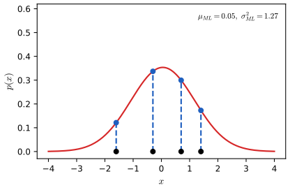
fig1_14. Download: PDF · SVGResult 1.6 (maximum likelihood for the Gaussian; Exercise 1.11) p. 27, (1.55), (1.56)
The log likelihood (1.54) has the unique global maximiser
\[ \mu_{\mathrm{ML}}=\frac1N\sum_{n=1}^{N}x_n,\qquad\text{(1.55)}\qquad \sigma^2_{\mathrm{ML}}=\frac1N\sum_{n=1}^{N}(x_n-\mu_{\mathrm{ML}})^2 , \tag{1.56} \]the sample mean and the sample variance measured with respect to the sample mean (provided the \(x_n\) are not all equal, so that \(\sigma^2_{\mathrm{ML}}>0\)).
Proof
Set \(\partial/\partial\mu\) of (1.54) to zero: \(\frac1{\sigma^2}\sum_n(x_n-\mu)=0\), so \(\mu=\frac1N\sum_nx_n\), whatever \(\sigma^2\) is; this is (1.55), and the equation for \(\mu\) does not involve \(\sigma^2\), so the joint maximisation can be done in two steps: first \(\mu\), then \(\sigma^2\). Differentiate (1.54) with respect to \(\sigma^2\): \(\frac{1}{2\sigma^4}\sum_n(x_n-\mu)^2\)
It is the global maximum. Put \(\beta=1/\sigma^2\) and \(S(\mu)=\sum_n(x_n-\mu)^2\). Then (1.54) is \(-\tfrac\beta2S(\mu)+\tfrac N2\ln\beta\)
Result 1.7 (expectations of products of samples; Exercise 1.12) p. 60, (1.130)
If \(x_n,x_m\) are independent draws from \(\mathcal{N}(\mu,\sigma^2)\) (for \(n\neq m\)), or the same draw (\(n=m\)), then \(\E[x_nx_m]=\mu^2+I_{nm}\sigma^2\), where \(I_{nm}=1\) if \(n=m\) and \(0\) otherwise.
Proof
If \(n=m\), \(\E[x_n^2]=\mu^2+\sigma^2\) by (1.50). If \(n\neq m\), independence gives \(\E[x_nx_m]=\E[x_n]\E[x_m]=\mu^2\) by (1.49) (Result 1.3(c)).∎
Result 1.8 (maximum likelihood is biased for the variance; Exercises 1.12, 1.13) pp. 27–28, (1.57)–(1.59)
Over data sets of \(N\) i.i.d. draws from \(\mathcal{N}(\mu,\sigma^2)\),
\[ \E[\mu_{\mathrm{ML}}]=\mu,\qquad\text{(1.57)}\qquad \E[\sigma^2_{\mathrm{ML}}]=\Big(\frac{N-1}{N}\Big)\sigma^2, \tag{1.58} \]so \(\sigma^2_{\mathrm{ML}}\) systematically under-estimates the variance, and \(\widetilde\sigma^2\)
Proof
(1.57): \(\E[\mu_{\mathrm{ML}}]=\frac1N\sum_n\E[x_n]=\mu\). For (1.58), expand the square in (1.56): \(\sigma^2_{\mathrm{ML}}\)
Therefore \(\E[\sigma^2_{\mathrm{ML}}]\)
Intuition (Figure 1.15). The sample mean is, by construction, the point that minimises \(\sum_n(x_n-m)^2\) over \(m\), so \(\sum_n(x_n-\mu_{\mathrm{ML}})^2\)
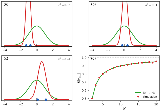
fig1_15. Download: PDF · SVGThe bias disappears as \(N\to\infty\) and is harmless for large \(N\), but it is the one-variable version of the over-fitting seen in Figure 1.4: maximum likelihood fits the noise. In a model with many parameters the same effect is large (the book returns to it in Section 3.4). The same happens in curve fitting: the residual sum of squares at \(\mathbf{w}_{\mathrm{ML}}\) has expectation \((N-M-1)\sigma^2\) when the model is correct, so the maximum likelihood noise variance (1.63) is too small by the factor \((N-M-1)/N\) (Chapter 3).
1.2.5 Curve fitting re-visited
pp. 28–30 Now give the curve-fitting problem a probabilistic model. Assume that, given \(x\), the target \(t\) is Gaussian with mean the polynomial \(y(x,\mathbf{w})\) of (1.1) and precision \(\beta\) (Figure 1.16):
\[ p(t\given x,\mathbf{w},\beta)=\mathcal{N}\big(t\given y(x,\mathbf{w}),\beta^{-1}\big). \tag{1.60} \]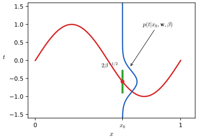
fig1_16. Download: PDF · SVGFor i.i.d. training data \(\{\mathbf{x},\mathbf{t}\}\) the likelihood and log likelihood are
\[ p(\mathbf{t}\given\mathbf{x},\mathbf{w},\beta)=\prod_{n=1}^{N}\mathcal{N}\big(t_n\given y(x_n,\mathbf{w}),\beta^{-1}\big),\tag{1.61} \] \[ \ln p(\mathbf{t}\given\mathbf{x},\mathbf{w},\beta)=-\frac\beta2\sum_{n=1}^{N}\{y(x_n,\mathbf{w})-t_n\}^2+\frac N2\ln\beta-\frac N2\ln(2\pi). \tag{1.62} \]Result 1.9 (least squares is maximum likelihood; \(\beta_{\mathrm{ML}}\)) pp. 29–30, (1.62)–(1.64)
Maximising (1.62) over \(\mathbf{w}\) is equivalent to minimising the sum-of-squares error (1.2): \(\mathbf{w}_{\mathrm{ML}}=\mathbf{w}^\star\) of Result 1.1. Maximising over \(\beta\) then gives
\[ \frac{1}{\beta_{\mathrm{ML}}}=\frac1N\sum_{n=1}^{N}\{y(x_n,\mathbf{w}_{\mathrm{ML}})-t_n\}^2=\frac{2E(\mathbf{w}_{\mathrm{ML}})}{N}=E_{\mathrm{RMS}}^2, \tag{1.63} \]and the predictive distribution with the maximum likelihood parameters is
\[ p(t\given x,\mathbf{w}_{\mathrm{ML}},\beta_{\mathrm{ML}})=\mathcal{N}\big(t\given y(x,\mathbf{w}_{\mathrm{ML}}),\beta_{\mathrm{ML}}^{-1}\big). \tag{1.64} \]Proof
In (1.62) the last two terms do not depend on \(\mathbf{w}\) and \(\beta/2>0\) is a positive constant, so \(\argmax_{\mathbf{w}}\ln p\)
Interpretation: \(1/\beta_{\mathrm{ML}}\) is the squared RMS error of Definition 1.1. By the bias of Result 1.8, applied to the residuals, it under-estimates the noise variance when \(M+1\) is not small compared with \(N\); at \(M=9\), \(N=10\) it is zero, which is the over-fit.
Take the next step towards a Bayesian treatment and put a Gaussian prior on the coefficients, with precision \(\alpha\) (a hyperparameter, since it controls the distribution of the parameters):
\[ p(\mathbf{w}\given\alpha)=\mathcal{N}(\mathbf{w}\given\mathbf{0},\alpha^{-1}\mathbf{I})=\Big(\frac{\alpha}{2\pi}\Big)^{(M+1)/2}\exp\Big\{-\frac\alpha2\mathbf{w}^\T\mathbf{w}\Big\}. \tag{1.65} \]By Bayes' theorem, the posterior is proportional to likelihood times prior,
\[ p(\mathbf{w}\given\mathbf{x},\mathbf{t},\alpha,\beta)\propto p(\mathbf{t}\given\mathbf{x},\mathbf{w},\beta)\,p(\mathbf{w}\given\alpha), \tag{1.66} \]and the maximum posterior (MAP) estimate is its maximiser.
Result 1.10 (MAP estimation is regularised least squares, \(\lambda=\alpha/\beta\)) p. 30, (1.66), (1.67)
The MAP estimate minimises
\[ \frac\beta2\sum_{n=1}^{N}\{y(x_n,\mathbf{w})-t_n\}^2+\frac\alpha2\mathbf{w}^\T\mathbf{w}, \tag{1.67} \]which is \(\beta\) times the regularised error (1.4) with \(\lambda=\alpha/\beta\). Hence \(\mathbf{w}_{\mathrm{MAP}}\)
Proof
Take \(-\ln\) of (1.66) and insert (1.62) and (1.65): \(-\ln p(\mathbf{w}\given\mathbf{x},\mathbf{t},\alpha,\beta)\)
So the regularisation parameter has a meaning: a large prior precision \(\alpha\) (a confident prior that the coefficients are small) or a small noise precision \(\beta\) (noisy data, so the data are less trusted) means strong regularisation. Note that MAP is still a point estimate: it is not yet Bayesian.
1.2.6 Bayesian curve fitting
pp. 30–32 A fully Bayesian treatment applies the sum and product rules consistently, which means integrating over \(\mathbf{w}\) rather than picking one value. Given the training data \(\{\mathbf{x},\mathbf{t}\}\) and a new input \(x\), the predictive distribution of the new target \(t\) is (taking \(\alpha,\beta\) as fixed and known)
\[ p(t\given x,\mathbf{x},\mathbf{t})=\int p(t\given x,\mathbf{w})\,p(\mathbf{w}\given\mathbf{x},\mathbf{t})\,\d\mathbf{w}. \tag{1.68} \]Here \(p(t\given x,\mathbf{w})\) is (1.60) and the posterior is (1.66) normalised. The book states that both are Gaussian and that the integral can be done analytically:
Result 1.11 (Bayesian polynomial curve fitting: posterior and predictive distribution) pp. 31–32, (1.68)–(1.72)
With the Gaussian likelihood (1.61) and the Gaussian prior (1.65), the posterior of \(\mathbf{w}\) is Gaussian, \(p(\mathbf{w}\given\mathbf{x},\mathbf{t})\)
where \(\bm\phi(x)\) has elements \(\phi_i(x)=x^i\), \(i=0,\dots,M\). Erratum. Early printings of (1.72) have \(\bm\phi(x_n)\bm\phi(x)^\T\), with the index \(n\) missing on the second factor; the correct form is as above.
Proof
Posterior. The log posterior is, up to terms independent of \(\mathbf{w}\) (from (1.61), (1.65) and (1.66), with \(y(x_n,\mathbf{w})=\mathbf{w}^\T\bm\phi(x_n)\)),
\[ \ln p(\mathbf{w}\given\mathbf{x},\mathbf{t})=-\frac\beta2\sum_n\big(t_n-\mathbf{w}^\T\bm\phi(x_n)\big)^2-\frac\alpha2\mathbf{w}^\T\mathbf{w}+\mathrm{const}=-\frac12\mathbf{w}^\T\Big[\alpha\mathbf{I}+\beta\sum_n\bm\phi(x_n)\bm\phi(x_n)^\T\Big]\mathbf{w}+\beta\,\mathbf{w}^\T\sum_n\bm\phi(x_n)t_n+\mathrm{const}. \]This is a quadratic in \(\mathbf{w}\) with a negative definite quadratic part. Completing the square: \(-\tfrac12\mathbf{w}^\T\mathbf{S}^{-1}\mathbf{w}\)
Predictive distribution. For a new input, \(t=\bm\phi(x)^\T\mathbf{w}+\varepsilon\) with \(\varepsilon\sim\mathcal{N}(0,\beta^{-1})\) independent of \(\mathbf{w}\) (this is (1.60)); (1.68) is the distribution of \(t\) when \(\mathbf{w}\) is drawn from the posterior. A linear function of a Gaussian vector is Gaussian: \(\bm\phi(x)^\T\mathbf{w}\)
The variance (1.71) depends on \(x\): its first term \(\beta^{-1}\) is the noise already present in the maximum likelihood predictive (1.64); the second term, \(\bm\phi(x)^\T\mathbf{S}\bm\phi(x)\ge0\), is the uncertainty about \(\mathbf{w}\) and is the new, Bayesian contribution. It is small near the data and large in gaps and away from them, and it shrinks to zero as \(N\to\infty\) (then \(\mathbf{S}\to\mathbf{0}\)), leaving only the noise. Unlike the maximum likelihood fit, the Bayesian predictive remains sensible for \(M=9\), \(N=10\) because the prior stops the coefficients from running away (Chapter 3 develops this and shows how \(\alpha\) and \(\beta\) can be inferred from the data too). The number of parameters can exceed the number of data points without over-fitting.
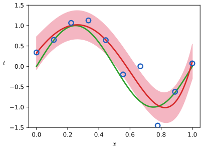
fig1_17. Download: PDF · SVG1.3 Model selection
pp. 32–34 Least squares and maximum likelihood fit the training data better the more complex the model, so the training error cannot choose the complexity (Figure 1.5). Complexity must be set against data that were not used to fit. With plentiful data one splits them into a training set and a validation set (hold-out set) and picks the order \(M\), or the regularisation \(\lambda\), with the smallest validation error; since the validation set is then used to choose, a third test set is kept untouched for the final performance estimate. When data are scarce this is wasteful, and a small validation set gives a noisy estimate.
S-fold cross-validation (Stone, 1974) (Figure 1.18) partitions the data into \(S\) groups, trains on \(S-1\) of them, evaluates on the held-out group, repeats for all \(S\) choices of the held-out group and averages the \(S\) scores. A proportion \((S-1)/S\) of the data is used for training, and every point is used for validation once. The extreme \(S=N\) is the leave-one-out technique. Drawbacks: the cost grows by the factor \(S\) (a problem when one training run is expensive), and with several complexity parameters (e.g. several regularisation coefficients) the number of settings to try may be exponential in their number.
An alternative is a criterion that uses only the training data and penalises complexity. The Akaike information criterion (Akaike, 1974) selects the model for which
\[ \ln p(\mathcal{D}\given\mathbf{w}_{\mathrm{ML}})-M \tag{1.73} \]is largest, with \(M\) the number of adjustable parameters; the Bayesian information criterion (Schwarz, 1978) replaces the penalty \(M\) by \(\tfrac12M\ln N\) (Section 4.4.1). Such criteria ignore the uncertainty of the parameters and tend to favour overly simple models; a fully Bayesian treatment (Section 3.4) gives the penalty automatically.
Filling the gap 1.3: where the penalties in AIC and BIC come from (outline) p. 33, (1.73)
The book quotes (1.73) without justification and refers to Section 4.4.1 for BIC. Here are the two heuristic arguments, in outline.
Derivation (outline)
AIC: the optimism of the maximised likelihood. Let the data be i.i.d. from \(p_0\) and assume the model family \(\{p(\cdot\given\bm\theta)\}\), \(\bm\theta\in\mathbb{R}^M\), contains \(p_0=p(\cdot\given\bm\theta_0)\) (and is regular). We want a model with large expected log likelihood on new data, \(\E_{\mathrm{new}}[\ln p(x\given\hat{\bm\theta})]\), which is a KL-divergence-based measure of how close \(p(\cdot\given\hat{\bm\theta})\) is to \(p_0\) up to a constant (see Section 1.6.1). The in-sample log likelihood \(\ell(\hat{\bm\theta})\)
BIC: the evidence with a Laplace approximation. The Bayesian model comparison criterion is the evidence \(p(\mathcal{D}\given\mathcal{M})\)
For i.i.d. data \(\mathbf{A}\approx N\mathbf{F}\), so \(\ln|\mathbf{A}|=M\ln N+\ln|\mathbf{F}|\); dropping the terms that do not grow with \(N\) leaves \(\ln p(\mathcal{D}\given\bm\theta_{\mathrm{ML}})\)
1.4 The curse of dimensionality
pp. 33–38 The sine example has one input. Real problems have many. Figure 1.19 shows 100 points of the oil-flow data (Appendix A of the book) in two of its twelve measurements, coloured by the flow regime (homogeneous, annular, laminar). A tempting classifier is to divide the plane into a regular grid and give a new point the majority class of its cell (Figure 1.20), but the number of cells grows as \(c^D\) when each axis is cut into \(c\) pieces (Figure 1.21): with \(D=12\) variables one would need exponentially many cells and, to have training points in each, exponentially much data.
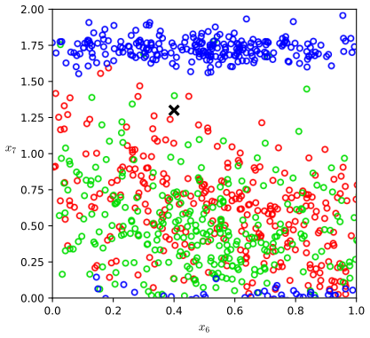
fig1_19. Download: PDF · SVG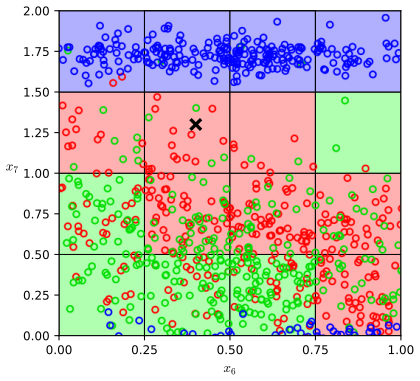
fig1_20. Download: PDF · SVG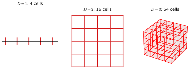
fig1_21. Download: PDF · SVGPolynomials. Extend the cubic to \(D\) inputs:
\[ y(\mathbf{x},\mathbf{w})=w_0+\sum_{i=1}^{D}w_ix_i+\sum_{i=1}^{D}\sum_{j=1}^{D}w_{ij}x_ix_j+\sum_{i=1}^{D}\sum_{j=1}^{D}\sum_{k=1}^{D}w_{ijk}x_ix_jx_k . \tag{1.74} \]Result 1.12 (counting the coefficients of a polynomial in \(D\) variables; Exercises 1.14–1.16) pp. 36, 60–61, (1.131)–(1.139)
The order-\(M\) term of a polynomial in \(D\) variables has \(n(D,M)\)
Proof (a direct counting argument; the induction of the exercises is in Exercise 1.15 and 1.16)
Because the monomials \(x_{i_1}\cdots x_{i_M}\) are invariant under reordering of the indices, the coefficients \(w_{i_1\dots i_M}\) can be taken symmetric, and the independent ones correspond one-to-one to the distinct monomials of degree exactly \(M\), i.e. to multisets of size \(M\) drawn from \(D\) variables. A multiset is described by the multiplicities \(m_1,\dots,m_D\ge0\) with \(\sum_im_i=M\); by stars and bars these number \(\binom{M+D-1}{M}\). Monomials of degree \(\le M\) correspond to multiplicities with \(\sum_{i=1}^{D}m_i\le M\), i.e. with a slack variable \(m_{D+1}=M-\sum m_i\ge0\) to \(D+1\) multiplicities summing to \(M\): \(\binom{M+D}{M}\). For \(D\gg M\), \((D+M)!/D!=(D+1)\cdots(D+M)\approx D^M\); for \(M\gg D\), \((D+M)!/M!\approx M^D\). Numbers: \(\binom{13}{3}=286\), \(\binom{103}{3}\)
Geometry. Our intuition from three dimensions also fails. The volume of a sphere of radius \(r\) in \(D\) dimensions must scale as \(r^D\) (scaling every coordinate by \(r\) multiplies volumes by the Jacobian determinant \(r^D\)), so \(V_D(r)=K_Dr^D\) (1.75) and the fraction of a unit sphere's volume that lies in the shell \(1-\epsilon\le\|\mathbf{x}\|\le1\) is
\[ \frac{V_D(1)-V_D(1-\epsilon)}{V_D(1)}=1-(1-\epsilon)^D, \tag{1.76} \]which tends to 1 for fixed \(\epsilon\) as \(D\to\infty\) (Figure 1.22): in high dimensions almost all of the volume of a sphere lies in a thin skin near the surface.
Result 1.13 (volume of the sphere and of the shell; Exercises 1.18, 1.19) pp. 37, 62, (1.76), (1.143)–(1.146)
The surface area of the unit sphere in \(D\) dimensions is \(S_D=2\pi^{D/2}/\Gamma(D/2)\) and the volume of the unit ball is \(V_D=S_D/D\), so \(K_D=V_D\). The fraction (1.76) equals \(0.0199,\ 0.0956,\ 0.634,\ 0.99996\) for \(\epsilon=0.01\) and \(D=2,10,100,1000\). The ratio of the volume of the sphere of radius \(a\) to that of the circumscribing cube of side \(2a\) is \(\pi^{D/2}/(D\,2^{D-1}\Gamma(D/2))\to0\) as \(D\to\infty\), while the corner is at distance \(\sqrt D\) times the distance to the centre of a face: most of the volume of a cube is in its \(2^D\) corners.
Proof
The formula (1.76) is exact: \(V_D(1)-V_D(1-\epsilon)=K_D(1-(1-\epsilon)^D)\). The values are \(1-0.99^D\). For \(S_D\), \(V_D\) and the cube ratio see Exercise 1.18 and Exercise 1.19, where they are derived (via the Gaussian integral of Result 1.4 in \(D\) dimensions).∎
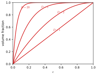
fig1_22. Download: PDF · SVGResult 1.14 (radial density of a high-dimensional Gaussian; Exercise 1.20) pp. 37–38, 63, (1.147)–(1.149)
Let \(p(\mathbf{x})\)
a normalised density in \(r\) with a single stationary point, at \(\hat r=\sqrt{D-1}\,\sigma\simeq\sqrt D\sigma\), a maximum, where \(p(\hat r+\epsilon)\)
Erratum. Early printings of (1.149) have the exponent \(-3\epsilon^2/2\sigma^2\); the correct exponent is \(-\epsilon^2/\sigma^2\).
Proof
The shell. The shell between radii \(r\) and \(r+\epsilon\) has volume \(V_D((r+\epsilon)^D-r^D)\)
Normalised. With \(u=r^2/2\sigma^2\), \(\int_0^\infty r^{D-1}\mathrm{e}^{-r^2/2\sigma^2}\d r\)
Stationary point. \(\ln p(r)=(D-1)\ln r-r^2/2\sigma^2+\mathrm{const}\), so \(\frac{\d}{\d r}\ln p\)
Density at the origin. \(p(\mathbf{0})=(2\pi\sigma^2)^{-D/2}\) and on the shell \(\|\mathbf{x}\|=\hat r\) \(p\)
As a check, \(\E[r^2]=\sum_{i=1}^D\E[x_i^2]=D\sigma^2\) exactly, consistent with a concentration of the mass at \(r\simeq\sqrt D\sigma\).∎
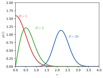
fig1_23. Download: PDF · SVGThese properties matter in later chapters: Bayesian inference over many parameters and sampling (Chapter 11) must take account of the fact that the region of high density is not where most of the probability mass is. The curse is not fatal for pattern recognition, for two reasons: real data usually lie near a lower-dimensional manifold (e.g. images of one object in varying position and orientation have only three degrees of freedom, whatever the number of pixels), and real data are locally smooth, so that local interpolation works.
1.5 Decision theory
pp. 38–48 Probability theory describes uncertainty; decision theory says what to do with it. Take medical diagnosis: from an X-ray image \(\mathbf{x}\) decide whether a patient has cancer (\(\mathcal{C}_1\)) or not (\(\mathcal{C}_2\)). The inference problem is to determine the joint distribution \(p(\mathbf{x},\mathcal{C}_k)\), equivalently the posterior probabilities
\[ p(\mathcal{C}_k\given\mathbf{x})=\frac{p(\mathbf{x}\given\mathcal{C}_k)\,p(\mathcal{C}_k)}{p(\mathbf{x})}, \tag{1.77} \]with \(p(\mathcal{C}_k)\) the prior and \(p(\mathcal{C}_k\given\mathbf{x})\) the posterior probability of class \(k\) after seeing the image. The decision step then turns these probabilities into an assignment, which should be the optimal one under the criterion chosen (see Berger, 1985, for a full account). The key point of the section is that, once the posteriors are known, the decision is simple, and different criteria give different decisions from the same posteriors.
1.5.1 Minimizing the misclassification rate
pp. 39–40 Divide the input space into decision regions \(\mathcal{R}_k\) (not necessarily connected); points in \(\mathcal{R}_k\) are assigned to \(\mathcal{C}_k\); the boundaries are decision boundaries or surfaces. For two classes a mistake occurs when \(\mathbf{x}\in\mathcal{R}_1\) belongs to \(\mathcal{C}_2\) or vice versa:
\[ p(\text{mistake})=p(\mathbf{x}\in\mathcal{R}_1,\mathcal{C}_2)+p(\mathbf{x}\in\mathcal{R}_2,\mathcal{C}_1)=\int_{\mathcal{R}_1}p(\mathbf{x},\mathcal{C}_2)\d\mathbf{x}+\int_{\mathcal{R}_2}p(\mathbf{x},\mathcal{C}_1)\d\mathbf{x}. \tag{1.78} \]For \(K\) classes it is easier to maximise the probability of being correct:
\[ p(\text{correct})=\sum_{k=1}^{K}p(\mathbf{x}\in\mathcal{R}_k,\mathcal{C}_k)=\sum_{k=1}^{K}\int_{\mathcal{R}_k}p(\mathbf{x},\mathcal{C}_k)\d\mathbf{x}. \tag{1.79} \]Result 1.15 (the minimum-misclassification-rate rule) pp. 39–40, (1.78), (1.79)
(1.79) is maximised, and (1.78) minimised, by assigning each \(\mathbf{x}\) to the class with the largest joint probability \(p(\mathbf{x},\mathcal{C}_k)\), equivalently the largest posterior \(p(\mathcal{C}_k\given\mathbf{x})\). The minimum error probability is \(p(\text{mistake})\)
Proof
The regions \(\mathcal{R}_k\) partition the input space, so each \(\mathbf{x}\) is counted in exactly one integral of (1.79), whose integrand there is \(p(\mathbf{x},\mathcal{C}_{k(\mathbf{x})})\) if \(\mathbf{x}\) is assigned to \(\mathcal{C}_{k(\mathbf{x})}\). The integrand at every \(\mathbf{x}\) is at most \(\max_kp(\mathbf{x},\mathcal{C}_k)\), with equality if and only if \(k(\mathbf{x})\) is a maximiser, and the assignments at different points can be chosen independently. Hence the integral is largest for the assignment \(k(\mathbf{x})\)
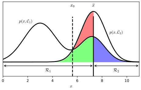
fig1_24. Download: PDF · SVG1.5.2 Minimizing the expected loss
pp. 41–42 Errors are not equally costly: telling a healthy patient that they may have cancer causes distress and further tests, while missing a cancer may cost a life. Introduce a loss matrix with element \(L_{kj}\), the loss incurred if the true class is \(\mathcal{C}_k\) and the assignment is \(\mathcal{C}_j\) (rows true, columns assigned; Figure 1.25: \(L=\begin{pmatrix}0&1000\\1&0\end{pmatrix}\) for (cancer, normal)). The true class is unknown, so average with respect to \(p(\mathbf{x},\mathcal{C}_k)\):
\[ \E[L]=\sum_k\sum_j\int_{\mathcal{R}_j}L_{kj}\,p(\mathbf{x},\mathcal{C}_k)\d\mathbf{x}. \tag{1.80} \]Result 1.16 (minimum expected loss; Exercises 1.22, 1.23) pp. 41–42, 63, (1.80), (1.81)
(1.80) is minimised by assigning each \(\mathbf{x}\) to the class \(j\) that minimises
\[ \sum_kL_{kj}\,p(\mathcal{C}_k\given\mathbf{x}). \tag{1.81} \]For the loss \(L_{kj}=1-I_{kj}\) (zero for a correct decision, one for any error) this is the largest-posterior rule of Result 1.15. With general class priors the same rule applies to the unnormalised quantity \(\sum_kL_{kj}\,p(\mathbf{x}\given\mathcal{C}_k)p(\mathcal{C}_k)\).
Proof
As in Result 1.15 each \(\mathbf{x}\) is assigned independently to some region \(\mathcal{R}_j\) and contributes \(\sum_kL_{kj}p(\mathbf{x},\mathcal{C}_k)\) to (1.80), so one minimises that over \(j\) at each \(\mathbf{x}\). Using \(p(\mathbf{x},\mathcal{C}_k)\)
Worked example: the cancer loss matrix p. 41, Figure 1.25
With \(L_{\text{cancer},\text{normal}}=1000\), \(L_{\text{normal},\text{cancer}}=1\) and zeros on the diagonal, (1.81) is \(1\cdot p(\text{normal}\given\mathbf{x})\) for the assignment "cancer" and \(1000\cdot p(\text{cancer}\given\mathbf{x})\) for "normal". Diagnose cancer when \(p(\text{normal}\given\mathbf{x})<1000\,p(\text{cancer}\given\mathbf{x})\), that is when \(p(\text{cancer}\given\mathbf{x})>1/1001\)
1.5.3 The reject option
pp. 42–43 Errors occur where the largest posterior is well below one, i.e. where the classes overlap. Rather than guess there, one may reject the input and leave it to a human expert or a further test. A simple rule: introduce a threshold \(\theta\) and reject all \(\mathbf{x}\) for which the largest posterior \(p(\mathcal{C}_k\given\mathbf{x})\le\theta\) (Figure 1.26). Setting \(\theta=1\) rejects everything, while for \(K\) classes \(\theta<1/K\) rejects nothing (the largest posterior is at least \(1/K\)).
Result 1.17 (reject option with a general loss; Exercise 1.24) pp. 43, 64
Let the loss for rejecting be \(\lambda\). Then the expected loss is minimised by assigning \(\mathbf{x}\) to the class \(j^\star\) minimising (1.81) if that minimum is less than \(\lambda\), and by rejecting \(\mathbf{x}\) otherwise. For \(L_{kj}=1-I_{kj}\) the rule is: reject if \(\max_kp(\mathcal{C}_k\given\mathbf{x})\)
Proof
At each \(\mathbf{x}\) the available actions are "assign to \(\mathcal{C}_j\)" with conditional expected loss \(\sum_kL_{kj}p(\mathcal{C}_k\given\mathbf{x})\), and "reject" with conditional expected loss \(\lambda\sum_kp(\mathcal{C}_k\given\mathbf{x})\)
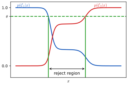
fig1_26. Download: PDF · SVG1.5.4 Inference and decision
pp. 42–46 The classification problem splits into an inference stage (learn a model of \(p(\mathcal{C}_k\given\mathbf{x})\)) and a decision stage (use it optimally). Three approaches, in decreasing order of complexity:
- Generative models. Model the class-conditional densities \(p(\mathbf{x}\given\mathcal{C}_k)\) and the priors \(p(\mathcal{C}_k)\), then use Bayes' theorem \[ p(\mathcal{C}_k\given\mathbf{x})=\frac{p(\mathbf{x}\given\mathcal{C}_k)\,p(\mathcal{C}_k)}{p(\mathbf{x})},\qquad\text{(1.82)}\qquad p(\mathbf{x})=\sum_kp(\mathbf{x}\given\mathcal{C}_k)\,p(\mathcal{C}_k). \tag{1.83} \] Equivalently model the joint \(p(\mathbf{x},\mathcal{C}_k)\) and normalise. Sampling from the model generates synthetic inputs, hence the name; it also gives \(p(\mathbf{x})\), which detects outliers (new inputs with low density, for which predictions are unreliable). It is the most demanding approach: the densities may need many data in high dimensions (Section 1.4), though the posteriors may be simple (Figure 1.27).
- Discriminative models. Model \(p(\mathcal{C}_k\given\mathbf{x})\) directly and then decide. Less demanding, since one needs only the (often simple) boundary region.
- Discriminant functions. Learn a function \(f(\mathbf{x})\) that maps \(\mathbf{x}\) directly to a class label. Simplest, but it gives no posteriors.
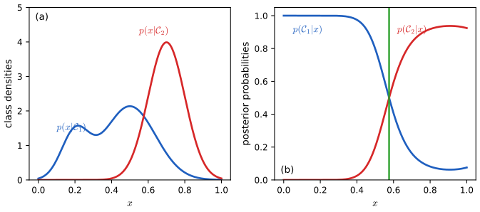
fig1_27. Download: PDF · SVGReasons to want posteriors rather than a discriminant function: (i) minimising risk: if the loss matrix changes (as in finance) one can re-decide without retraining; (ii) the reject option; (iii) compensating for class priors: in the X-ray problem cancer is rare (say 1 in 1000), and a classifier trained on a balanced sample has seen a distorted prior; (iv) combining models, e.g. one for X-ray images \(\mathbf{x}_I\) and another for blood data \(\mathbf{x}_B\).
Filling the gap 1.4: correcting for class priors, and combining models under conditional independence pp. 45–46, (1.84), (1.85)
The book describes both in words ("divide by the class fractions ... multiply by the population fractions"; "(1.85)"). Here are the two derivations.
Derivation
Priors. Suppose a classifier gives \(p_{\mathrm{bal}}(\mathcal{C}_k\given\mathbf{x})\) when trained on data with class fractions \(\pi^{\mathrm{bal}}_k\) (e.g. \(1/2,1/2\)), and the class-conditional densities \(p(\mathbf{x}\given\mathcal{C}_k)\) are the same in the population, whose true priors are \(\pi_k\). By Bayes, \(p(\mathbf{x}\given\mathcal{C}_k)\)
the common factor \(p_{\mathrm{bal}}(\mathbf{x})\) cancelling in the ratio: divide by the training fractions, multiply by the population fractions, normalise. It needs posteriors; it cannot be applied to a discriminant function.
Combining models. Assume that, within each class, the two kinds of data are independent: \(p(\mathbf{x}_I,\mathbf{x}_B\given\mathcal{C}_k)\)
where the last step uses \(p(\mathbf{x}_I\given\mathcal{C}_k)\)
1.5.5 Loss functions for regression
pp. 46–48 In regression the decision is a point estimate \(y(\mathbf{x})\) of \(t\) for each input, and a loss \(L(t,y(\mathbf{x}))\) is incurred; its average is
\[ \E[L]=\iint L(t,y(\mathbf{x}))\,p(\mathbf{x},t)\d\mathbf{x}\d t. \tag{1.86} \]A common choice is the squared loss \(L=\{y(\mathbf{x})-t\}^2\), giving \(\E[L]\)
Result 1.18 (the regression function is the conditional mean; Exercises 1.25, 1.26) pp. 46–47, 64, (1.87)–(1.90), (1.151)
The squared-loss risk (1.87) is minimised by
\[ y(\mathbf{x})=\frac{\int t\,p(\mathbf{x},t)\d t}{p(\mathbf{x})}=\int t\,p(t\given\mathbf{x})\d t=\E_t[t\given\mathbf{x}], \tag{1.89} \]the regression function, and for any other \(y(\mathbf{x})\)
\[ \E[L]=\int\{y(\mathbf{x})-\E[t\given\mathbf{x}]\}^2p(\mathbf{x})\d\mathbf{x}+\int\var[t\given\mathbf{x}]\,p(\mathbf{x})\d\mathbf{x}. \tag{1.90} \]The second term is the irreducible noise and does not depend on \(y\). For vector targets \(\mathbf{t}\) with loss \(\|\mathbf{y}(\mathbf{x})-\mathbf{t}\|^2\) the minimiser is again \(\mathbf{y}(\mathbf{x})\)
Proof (calculus of variations, and by completing the square)
Variational derivation. Let \(\eta(\mathbf{x})\) be an arbitrary test function and consider \(\E[L]\) at \(y+\epsilon\eta\) (see the calculus of variations). Then
\[ \frac{\d}{\d\epsilon}\E[L]\Big|_{\epsilon=0}=2\iint\{y(\mathbf{x})-t\}\,\eta(\mathbf{x})\,p(\mathbf{x},t)\d t\d\mathbf{x}=2\int\eta(\mathbf{x})\Big[\int\{y(\mathbf{x})-t\}p(\mathbf{x},t)\d t\Big]\d\mathbf{x}. \]At a minimum this vanishes for every \(\eta\), which forces the bracket (the functional derivative (1.88)) to vanish at every \(\mathbf{x}\) with \(p(\mathbf{x})>0\). Solving, \(y(\mathbf{x})\int p(\mathbf{x},t)\d t\)
Completing the square, which also shows it is a minimum. Write \(\E[t\given\mathbf{x}]\) for \(\E_t[t\given\mathbf{x}]\). Then
\[ \{y(\mathbf{x})-t\}^2=\{y(\mathbf{x})-\E[t\given\mathbf{x}]\}^2+2\{y(\mathbf{x})-\E[t\given\mathbf{x}]\}\{\E[t\given\mathbf{x}]-t\}+\{\E[t\given\mathbf{x}]-t\}^2 . \]Integrate over \(t\) with weight \(p(t\given\mathbf{x})\): the cross term is proportional to \(\int\{\E[t\given\mathbf{x}]\)
Vector targets (Exercises 1.25, 1.26). Here \(\E[L]\)
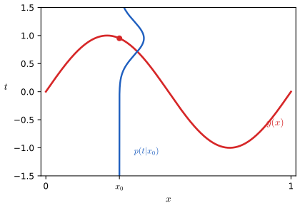
fig1_28. Download: PDF · SVGHere too there are three approaches: determine the joint \(p(\mathbf{x},t)\), normalise to \(p(t\given\mathbf{x})\) and take its mean (1.89); determine \(p(t\given\mathbf{x})\) directly (what Section 1.2.5 does for curve fitting); or fit \(y(\mathbf{x})\) directly to the data. The squared loss is not the only choice, and can be poor when \(p(t\given\mathbf{x})\) is multimodal, as often happens in inverse problems (Section 5.6; the mean of two modes may lie between them). A simple generalisation is the Minkowski loss
\[ \E[L_q]=\iint|y(\mathbf{x})-t|^q\,p(\mathbf{x},t)\d\mathbf{x}\d t, \tag{1.91} \]which is the squared loss for \(q=2\) (Figure 1.29).
Result 1.19 (Minkowski loss: mean, median, mode; Exercise 1.27) pp. 48, 64, (1.91)
For \(q>1\) the minimiser \(y(\mathbf{x})\) of (1.91) satisfies \(\int|y\)
Proof
See Exercise 1.27 for the complete argument, including the limit \(q\to0\).∎
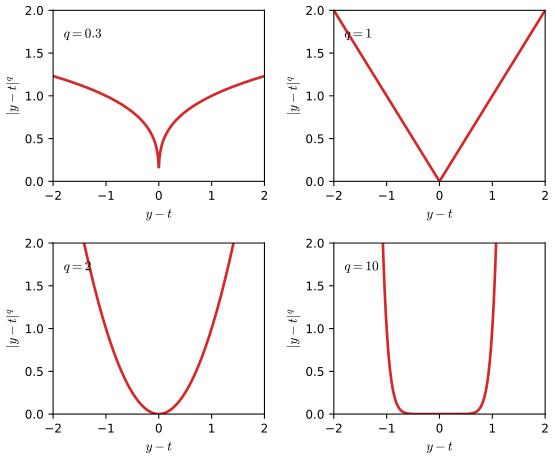
fig1_29. Download: PDF · SVG1.6 Information theory
pp. 48–58 How much information is received when we observe the value of a discrete random variable \(x\)? Learning that a very unlikely event happened is more informative than learning that a certain one did. So we want a function \(h(x)\), monotone in \(p(x)\), with \(h(x,y)=h(x)+h(y)\) for unrelated events; since independent events have \(p(x,y)=p(x)p(y)\), \(h\) must turn products into sums, and it follows (Exercise 1.28) that
\[ h(x)=-\log_2p(x), \tag{1.92} \]measured in bits (with natural logarithms, in nats; the book switches to natural logarithms from here on). The average information transmitted by a random variable is its entropy (Shannon, 1948)
\[ \mathrm{H}[x]=-\sum_xp(x)\log_2p(x), \tag{1.93} \]with the convention \(0\ln0=0\) (since \(p\ln p\to0\) as \(p\to0\)). Entropy is non-negative, and zero exactly when one outcome has probability 1.
Entropy as a count. A second motivation (Boltzmann). Place \(N\) identical objects into bins \(i=1,\dots,M\) with \(n_i\) in bin \(i\). The number of distinct arrangements of the distinguishable objects giving the occupation numbers \((n_i)\) is the multiplicity
\[ W=\frac{N!}{\prod_in_i!}, \tag{1.94} \]and the entropy is defined as the logarithm of the multiplicity, scaled:
\[ \mathrm{H}=\frac1N\ln W=\frac1N\ln N!-\frac1N\sum_i\ln n_i!. \tag{1.95} \]For \(N\to\infty\) with \(p_i=n_i/N\) fixed, Stirling's approximation \(\ln N!\simeq N\ln N-N\) (1.96) gives
\[ \mathrm{H}=\lim_{N\to\infty}\Big[\ln N-1-\frac1N\sum_i(n_i\ln n_i-n_i)\Big]=-\lim_{N\to\infty}\sum_i\Big(\frac{n_i}N\Big)\ln\Big(\frac{n_i}N\Big)=-\sum_ip_i\ln p_i , \tag{1.97} \]using \(\sum_in_i=N\) in the middle step: \(\frac1N\sum_in_i\ln n_i=\ln N+\sum_ip_i\ln p_i\). Writing \(p(x_i)=p_i\) for the probabilities of the states of a discrete variable \(X\), the entropy of the variable is \(\mathrm{H}[p]=-\sum_ip(x_i)\ln p(x_i)\) (1.98). Distributions sharply peaked on a few values have low entropy, those spread over many values high entropy (Figure 1.30).
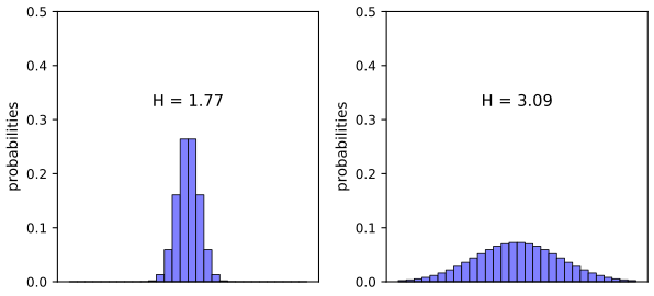
fig1_30. Download: PDF · SVGResult 1.20 (maximum entropy: the uniform distribution; Exercise 1.29) pp. 49–52, 64, (1.99), (1.100)
Among all distributions on \(M\) states, \(\mathrm{H}[p]\) is maximised uniquely by \(p(x_i)=1/M\), with \(\mathrm{H}=\ln M\); the minimum \(0\) is attained when one \(p_i=1\). Hence \(0\le\mathrm{H}[x]\le\ln M\).
Proof (Lagrange multiplier, and Jensen)
Lagrange multiplier. Maximise \(\mathrm{H}\) subject to the constraint \(\sum_ip(x_i)=1\) (see Lagrange multipliers), i.e. the stationary points of
\[ \widetilde{\mathrm{H}}=-\sum_ip(x_i)\ln p(x_i)+\lambda\Big(\sum_ip(x_i)-1\Big). \tag{1.99} \]\(\partial\widetilde{\mathrm{H}}/\partial p(x_i)\)
a negative definite diagonal matrix (\(I_{ij}\) the identity), so \(\widetilde{\mathrm H}\) is strictly concave on the probability simplex and the stationary point is the unique global maximum. Erratum. Early printings write \(\partial\widetilde{\mathrm H}\) instead of \(\partial^2\widetilde{\mathrm H}\) in the numerator of (1.100).
Jensen. With \(f=\ln\) concave (Jensen: \(\E[\ln u]\le\ln\E[u]\), toolkit): \(\mathrm{H}[x]\)
Differential entropy
For a continuous variable, divide the axis into bins of width \(\Delta\). By the mean value theorem there is \(x_i\) in the \(i\)th bin with \(\int_{i\Delta}^{(i+1)\Delta}p(x)\d x\)
using \(\sum_ip(x_i)\Delta=1\). Drop the term \(-\ln\Delta\) (it diverges as \(\Delta\to0\): specifying a continuous variable exactly takes infinitely many bits) and take \(\Delta\to0\); the first sum becomes a Riemann integral:
\[ \lim_{\Delta\to0}\Big\{-\sum_ip(x_i)\Delta\ln p(x_i)\Big\}=-\int p(x)\ln p(x)\d x, \tag{1.103} \]the differential entropy, \(\mathrm{H}[\mathbf{x}]\)
Result 1.21 (the Gaussian maximises the differential entropy; Exercises 1.34, 1.35) pp. 53–54, 65, (1.105)–(1.110)
(The maximum entropy principle: Jaynes, 1957.) Among all densities with \(\int p=1\), \(\int xp\,\d x=\mu\) and \(\int(x-\mu)^2p\,\d x=\sigma^2\) (1.105–1.107), the differential entropy is maximised by the Gaussian \(p(x)=\mathcal{N}(x\given\mu,\sigma^2)\) (1.109), whose entropy is
\[ \mathrm{H}[x]=\frac12\big\{1+\ln(2\pi\sigma^2)\big\}. \tag{1.110} \]The entropy increases with \(\sigma^2\): the broader the distribution the larger the entropy.
Proof (Lagrange multipliers and the calculus of variations; the maximum by the KL inequality)
Stationarity. Form the functional with one multiplier per constraint,
\[ -\int p\ln p\,\d x+\lambda_1\Big(\int p\,\d x-1\Big)+\lambda_2\Big(\int xp\,\d x-\mu\Big)+\lambda_3\Big(\int(x-\mu)^2p\,\d x-\sigma^2\Big). \]Its functional derivative (see the calculus of variations; the integrand depends on \(p(x)\) pointwise, so the functional derivative is the partial derivative of the integrand with respect to \(p\)) is \(-\ln p(x)-1+\lambda_1+\lambda_2x\)
Eliminating the multipliers. For \(p\) to be integrable we need \(\lambda_3<0\). Complete the square: \(\lambda_2x+\lambda_3(x-\mu)^2\)
It is the maximum. Let \(q\) be any density with the same mean and variance and \(g=\mathcal{N}(\cdot\given\mu,\sigma^2)\). Then \(-\int q\ln g\,\d x\)
Entropy of the Gaussian (Exercise 1.35). \(\mathrm{H}[g]\)
Conditional entropy
For a joint distribution \(p(\mathbf{x},\mathbf{y})\), the average additional information needed to specify \(\mathbf{y}\) once \(\mathbf{x}\) is known is the conditional entropy
\[ \mathrm{H}[\mathbf{y}\given\mathbf{x}]=-\iint p(\mathbf{y},\mathbf{x})\ln p(\mathbf{y}\given\mathbf{x})\d\mathbf{y}\d\mathbf{x}, \tag{1.111} \]and, by the product rule \(\ln p(\mathbf{x},\mathbf{y})\)
The information needed to describe \(\mathbf{x}\) and \(\mathbf{y}\) is that for \(\mathbf{x}\) plus that for \(\mathbf{y}\) given \(\mathbf{x}\).
1.6.1 Relative entropy and mutual information
pp. 55–58 Suppose the unknown distribution is \(p(\mathbf{x})\) and we model it by \(q(\mathbf{x})\). Coding with \(q\) instead of \(p\) costs, on average, an extra amount of information, the relative entropy or Kullback-Leibler divergence (Kullback and Leibler, 1951):
\[ \KL(p\|q)=-\int p(\mathbf{x})\ln q(\mathbf{x})\d\mathbf{x}-\Big(-\int p(\mathbf{x})\ln p(\mathbf{x})\d\mathbf{x}\Big)=-\int p(\mathbf{x})\ln\Big\{\frac{q(\mathbf{x})}{p(\mathbf{x})}\Big\}\d\mathbf{x}. \tag{1.113} \]It is not symmetric: \(\KL(p\|q)\neq\KL(q\|p)\) in general. To show that it is non-negative we need convexity. A function \(f\) is convex if every chord lies on or above it:
\[ f(\lambda a+(1-\lambda)b)\le\lambda f(a)+(1-\lambda)f(b),\qquad 0\le\lambda\le1, \tag{1.114} \]strictly convex if equality holds only at \(\lambda\in\{0,1\}\) (Figure 1.31). Examples: \(x\ln x\) for \(x>0\), \(-\ln x\), \(x^2\), \(\mathrm{e}^x\). By induction (Exercise 1.38) (1.114) extends to Jensen's inequality, for \(\lambda_i\ge0\), \(\sum_i\lambda_i=1\):
\[ f\Big(\sum_{i=1}^{M}\lambda_ix_i\Big)\le\sum_{i=1}^{M}\lambda_if(x_i), \tag{1.115} \]that is \(f(\E[x])\le\E[f(x)]\) (1.116), and for continuous variables \(f(\int xp(x)\d x)\le\int f(x)p(x)\d x\) (1.117). For concave \(f\) (such as \(\ln\)) the inequalities reverse.
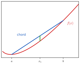
fig1_31. Download: PDF · SVGResult 1.22 (Gibbs' inequality: \(\KL(p\|q)\ge0\)) p. 56, (1.117), (1.118)
For densities \(p,q\), \(\KL(p\|q)\ge0\), with equality if and only if \(p(\mathbf{x})=q(\mathbf{x})\) almost everywhere. (The same holds for discrete distributions with sums.)
Proof (Jensen's inequality)
Apply Jensen (1.117) to the convex function \(f(u)=-\ln u\) with the random variable \(u=q(\mathbf{x})/p(\mathbf{x})\) under \(p\):
\[ \KL(p\|q)=-\int p(\mathbf{x})\ln\Big\{\frac{q(\mathbf{x})}{p(\mathbf{x})}\Big\}\d\mathbf{x}\ \ge\ -\ln\int q(\mathbf{x})\,\d\mathbf{x}=0, \tag{1.118} \]since \(\int p\cdot(q/p)\,\d\mathbf{x}\)
So \(\KL(p\|q)\) is a measure of dissimilarity (not a metric: not symmetric, no triangle inequality). Link with maximum likelihood. If \(p(\mathbf{x})\) is unknown and we model it by \(q(\mathbf{x}\given\bm\theta)\), minimising \(\KL(p\|q)\) over \(\bm\theta\) cannot be done directly, but with data \(\mathbf{x}_n\sim p\) the expectation over \(p\) is approximated by a sample average (1.35):
\[ \KL(p\|q)\simeq\frac1N\sum_{n=1}^{N}\{-\ln q(\mathbf{x}_n\given\bm\theta)+\ln p(\mathbf{x}_n)\}. \tag{1.119} \]The second term is independent of \(\bm\theta\) and the first is the negative log likelihood divided by \(N\): minimising this KL divergence is maximising the likelihood. (Erratum. Early printings omit the factor \(1/N\) in (1.119).)
Result 1.23 (mutual information) pp. 57–58, 66, (1.120), (1.121)
The mutual information of \(\mathbf{x}\) and \(\mathbf{y}\) is the KL divergence between the joint and the product of the marginals,
\[ \mathrm{I}[\mathbf{x},\mathbf{y}]\equiv\KL\big(p(\mathbf{x},\mathbf{y})\,\|\,p(\mathbf{x})p(\mathbf{y})\big)=-\iint p(\mathbf{x},\mathbf{y})\ln\Big(\frac{p(\mathbf{x})p(\mathbf{y})}{p(\mathbf{x},\mathbf{y})}\Big)\d\mathbf{x}\d\mathbf{y}. \tag{1.120} \]It satisfies \(\mathrm{I}[\mathbf{x},\mathbf{y}]\ge0\), with equality iff \(\mathbf{x}\) and \(\mathbf{y}\) are independent, and
\[ \mathrm{I}[\mathbf{x},\mathbf{y}]=\mathrm{H}[\mathbf{x}]-\mathrm{H}[\mathbf{x}\given\mathbf{y}]=\mathrm{H}[\mathbf{y}]-\mathrm{H}[\mathbf{y}\given\mathbf{x}]. \tag{1.121} \]Proof
Non-negativity and the equality case are Result 1.22 with \(q=p(\mathbf{x})p(\mathbf{y})\): they hold iff the joint equals the product of the marginals, i.e. independence. For (1.121), use \(\ln\frac{p(\mathbf{x})p(\mathbf{y})}{p(\mathbf{x},\mathbf{y})}\)
Interpretation: \(\mathrm{H}[\mathbf{x}]\) is the uncertainty about \(\mathbf{x}\) before, \(\mathrm{H}[\mathbf{x}\given\mathbf{y}]\) after, observing \(\mathbf{y}\), so the mutual information is the reduction in uncertainty about \(\mathbf{x}\) obtained from \(\mathbf{y}\): from a Bayesian viewpoint \(p(\mathbf{x})\) is the prior and \(p(\mathbf{x}\given\mathbf{y})\) the posterior after observing \(\mathbf{y}\). Since \(\mathrm{I}\ge0\), conditioning on average does not increase entropy: \(\mathrm{H}[\mathbf{x}\given\mathbf{y}]\)
Exercises
All 41 exercises of Chapter 1 (Bishop, 2006, pp. 58–66), restated in my own words, with complete solutions (hidden). Stars give the book's difficulty and "www" marks the exercises with official solutions. Many exercises are the derivations of the results above; those solutions summarise the argument and link to the full version. Where the official solution manual is incomplete or the book has an erratum, this is said.
Exercise 1.1 (★, www). Show that the coefficients minimising the sum-of-squares error (1.2) for the polynomial (1.1) solve \(\sum_jA_{ij}w_j=T_i\) with \(A_{ij}=\sum_n(x_n)^{i+j}\), \(T_i=\sum_n(x_n)^it_n\) (1.122, 1.123).
Solution
Differentiate: \(\partial E/\partial w_i\)
\({}=\sum_n\{\sum_jw_jx_n^j-t_n\}x_n^i\) \({}=\sum_jA_{ij}w_j-T_i\); set to zero. That the stationary point is the global minimiser, and unique when at least \(M+1\) of the \(x_n\) are distinct, is shown in Result 1.1. Exercise 1.2 (★). Write down the linear equations satisfied by the coefficients that minimise the regularised error (1.4).
Solution
The extra term \(\tfrac\lambda2\sum_jw_j^2\) adds \(\lambda w_i\) to \(\partial\widetilde E/\partial w_i\), so \(\sum_{j=0}^{M}(A_{ij}+\lambda\delta_{ij})w_j=T_i\), i.e. \((\bm\Phi^\T\bm\Phi+\lambda\mathbf{I})\mathbf{w}\)
\({}=\bm\Phi^\T\mathbf{t}\) (Result 1.2; if \(w_0\) is not penalised, the \(i=j=0\) diagonal entry is left unchanged). Exercise 1.3 (★★). Three boxes: red has 3 apples, 4 oranges, 3 limes; blue has 1 apple, 1 orange, 0 limes; green has 3 apples, 3 oranges, 4 limes. A box is chosen with \(p(r)=0.2\), \(p(b)=0.2\), \(p(g)=0.6\), then a fruit uniformly at random from it. (a) What is the probability of an apple? (b) Given that the fruit is an orange, what is the probability that it came from the green box?
Solution
Conditional probabilities of fruit given box: apple \(3/10,\ 1/2,\ 3/10\); orange \(4/10,\ 1/2,\ 3/10\) for \(r,b,g\). (a) By the sum and product rules \(p(a)\)
\({}=0.2\cdot0.3+0.2\cdot0.5+0.6\cdot0.3\) \({}=0.06+0.10+0.18\) \({}=0.34\). (b) \(p(o)\) \({}=0.2\cdot0.4+0.2\cdot0.5+0.6\cdot0.3\) \({}=0.08+0.10+0.18\) \({}=0.36\), and by Bayes' theorem \(p(g\given o)\) \({}=\frac{p(o\given g)p(g)}{p(o)}\) \({}=\frac{0.3\cdot0.6}{0.36}\) \({}=\frac12\). Exercise 1.4 (★★, www). Under a nonlinear change of variable \(x=g(y)\) the density transforms by (1.27). By differentiating (1.27), show that the maximum of the density in \(y\) is not in general at \(\hat y=g^{-1}(\hat x)\), and verify that it is for a linear transformation.
Solution
For \(g'>0\), \(p_y'(y)=p_x'(g(y))g'(y)^2+p_x(g(y))g''(y)\). At \(\hat y=g^{-1}(\hat x)\), \(p_x'(\hat x)=0\), so \(p_y'(\hat y)=p_x(\hat x)g''(\hat y)\neq0\) unless \(g''(\hat y)=0\); for linear \(g(y)=ay+b\) one has \(g''=0\) and \(p_y'(y)=a^2p_x'(ay+b)\), which vanishes at \(\hat y\). Full argument with an example: Filling the gap 1.2.
Exercise 1.5 (★). Using the definition (1.38) show that \(\var[f(x)]=\E[f(x)^2]-\E[f(x)]^2\) (1.39).
Solution
With \(\mu=\E[f]\) constant: \(\E[(f-\mu)^2]\)
\({}=\E[f^2]-2\mu\E[f]+\mu^2\) \({}=\E[f^2]-\mu^2\) (Result 1.3(a)). Exercise 1.6 (★). Show that independent variables have zero covariance.
Solution
If \(p(x,y)=p(x)p(y)\), \(\E[xy]=\iint xy\,p(x)p(y)=\E[x]\E[y]\), so \(\cov[x,y]=\E[xy]-\E[x]\E[y]=0\) (Result 1.3(c)). The converse is false (\(x\sim\mathcal{N}(0,1)\), \(y=x^2\)).
Exercise 1.7 (★★, www). Prove the normalisation (1.48) of the univariate Gaussian by squaring \(I=\int\exp(-x^2/2\sigma^2)\d x\), passing to polar coordinates and substituting \(u=r^2\), to obtain \(I=(2\pi\sigma^2)^{1/2}\) (1.126).
Solution
\(I^2\)
\({}=\iint\exp(-(x^2+y^2)/2\sigma^2)\d x\d y\) \({}=\int_0^{2\pi}\d\theta\int_0^\infty\mathrm{e}^{-r^2/2\sigma^2}r\,\d r\) \({}=2\pi\cdot\tfrac12\int_0^\infty\mathrm{e}^{-u/2\sigma^2}\d u\) \({}=2\pi\sigma^2\). Take the positive root, then shift by \(\mu\). Details in Result 1.4. Exercise 1.8 (★★, www). By a change of variables verify (1.49) \(\E[x]=\mu\). Then by differentiating the normalisation (1.127) with respect to \(\sigma^2\) verify (1.50), and show (1.51).
Solution
With \(y=x-\mu\): \(\E[x]\)
\({}=\mu\) \({}+\int y\,\mathcal{N}(y\given0,\sigma^2)\d y\) \({}=\mu\), the integral of an odd function. Differentiating \(\int\mathcal{N}\d x=1\) in \(\sigma^2\) gives \(\int[-\frac1{2\sigma^2}+\frac{(x-\mu)^2}{2\sigma^4}]\mathcal{N}\d x\) \({}=0\), so \(\E[(x-\mu)^2]=\sigma^2\); then \(\E[x^2]=\sigma^2+2\mu\E[x]-\mu^2=\mu^2+\sigma^2\) (1.50) and \(\var[x]=\E[x^2]-\E[x]^2=\sigma^2\) (1.51). See Result 1.5. Exercise 1.9 (★, www). Show that the mode of the Gaussian (1.46) is \(\mu\), and that of the multivariate Gaussian (1.52) is \(\bm\mu\).
Solution
\(\frac{\d}{\d x}\ln\mathcal{N}\)
\({}=-(x-\mu)/\sigma^2\) \({}=0\) only at \(x=\mu\), and the log density is a concave parabola. In \(D\) dimensions \(\nabla\ln\mathcal{N}\) \({}=-\bm\Sigma^{-1}(\mathbf{x}-\bm\mu)\) \({}=\mathbf{0}\) iff \(\mathbf{x}=\bm\mu\) (\(\bm\Sigma\) invertible), and \(\ln\mathcal{N}\) \({}=-\frac12(\mathbf{x}-\bm\mu)^\T\bm\Sigma^{-1}(\mathbf{x}-\bm\mu)\) \({}+\mathrm{const}\) \({}\le\mathrm{const}\) with equality only there (Result 1.5). Exercise 1.10 (★, www). If \(x\) and \(z\) are independent, show that \(\E[x+z]=\E[x]+\E[z]\) and \(\var[x+z]=\var[x]+\var[z]\).
Solution
\(\E[x+z]=\iint(x+z)p(x)p(z)=\E x+\E z\). \(\var[x+z]\)
\({}=\E[(x+z)^2]-(\E x+\E z)^2\) \({}=\var x+\var z+2(\E[xz]-\E x\E z)\) and the bracket is zero by independence (Result 1.3(d)). Exercise 1.11 (★). Set the derivatives of the Gaussian log likelihood (1.54) with respect to \(\mu\) and \(\sigma^2\) to zero to verify (1.55) and (1.56).
Solution
\(\partial/\partial\mu\): \(\frac1{\sigma^2}\sum_n(x_n-\mu)\)
\({}=0\) \({}\Rightarrow\mu_{\mathrm{ML}}\) \({}=\frac1N\sum x_n\). \(\partial/\partial\sigma^2\): \(\frac1{2\sigma^4}\sum_n(x_n-\mu)^2\) \({}-\frac N{2\sigma^2}\) \({}=0\) \({}\Rightarrow\sigma^2\) \({}=\frac1N\sum_n(x_n-\mu)^2\); inserting \(\mu_{\mathrm{ML}}\) gives (1.56). That this is the global maximum is shown in Result 1.6. Exercise 1.12 (★★, www). Show that \(\E[x_nx_m]=\mu^2+I_{nm}\sigma^2\) (1.130) for samples from a Gaussian, and hence prove (1.57) and (1.58).
Solution
For \(n=m\): \(\E[x_n^2]=\mu^2+\sigma^2\) by (1.50); for \(n\neq m\): independence gives \(\mu^2\). Then \(\E[\mu_{\mathrm{ML}}]=\mu\), \(\E[\mu_{\mathrm{ML}}^2]\)
\({}=\frac1{N^2}\sum_{n,m}(\mu^2+I_{nm}\sigma^2)\) \({}=\mu^2+\sigma^2/N\), and with \(\sigma^2_{\mathrm{ML}}\) \({}=\frac1N\sum x_n^2-\mu_{\mathrm{ML}}^2\), \(\E[\sigma^2_{\mathrm{ML}}]\) \({}=\mu^2+\sigma^2-\mu^2-\sigma^2/N\) \({}=\frac{N-1}N\sigma^2\) (Results 1.7 and 1.8). Exercise 1.13 (★). If the variance is estimated by (1.56) with \(\mu_{\mathrm{ML}}\) replaced by the true mean \(\mu\), show that the estimator is unbiased.
Solution
\(\E[\frac1N\sum_n(x_n-\mu)^2]\)
\({}=\frac1N\sum_n\var[x_n]\) \({}=\sigma^2\): the bias in (1.58) comes entirely from estimating \(\mu\) from the same data (Result 1.8). Exercise 1.14 (★★). Show that a square matrix \(w_{ij}\) is the sum of a symmetric and an anti-symmetric matrix; that \(\sum_{ij}w_{ij}x_ix_j\)
\({}=\sum_{ij}w^{\mathrm S}_{ij}x_ix_j\); and that a symmetric \(D\times D\) matrix has \(D(D+1)/2\) independent elements. Solution
Put \(w^{\mathrm S}_{ij}=\frac12(w_{ij}+w_{ji})\) and \(w^{\mathrm A}_{ij}=\frac12(w_{ij}-w_{ji})\): then \(w^{\mathrm S}_{ij}=w^{\mathrm S}_{ji}\), \(w^{\mathrm A}_{ij}=-w^{\mathrm A}_{ji}\) and \(w_{ij}=w^{\mathrm S}_{ij}+w^{\mathrm A}_{ij}\). Relabelling the summation indices, \(\sum_{ij}w^{\mathrm A}_{ij}x_ix_j\)
\({}=\sum_{ij}w^{\mathrm A}_{ji}x_jx_i\) \({}=-\sum_{ij}w^{\mathrm A}_{ij}x_ix_j\), so it equals its own negative and vanishes. Hence only \(\mathbf{w}^{\mathrm S}\) matters. A symmetric matrix is fixed by its diagonal (\(D\) entries) and the entries above it (\(D(D-1)/2\)): \(D+D(D-1)/2=D(D+1)/2\). Exercise 1.15 (★★★, www). The \(M\)th order term of a polynomial in \(D\) variables is \(\sum_{i_1}\cdots\sum_{i_M}w_{i_1\dots i_M}x_{i_1}\cdots x_{i_M}\) (1.133). Show that its redundancy can be removed by restricting to \(i_M\le i_{M-1}\le\dots\le i_1\) (1.134); that the number of independent parameters satisfies \(n(D,M)=\sum_{i=1}^Dn(i,M-1)\) (1.135); that \(\sum_{i=1}^D\frac{(i+M-2)!}{(i-1)!(M-1)!}\)
\({}=\frac{(D+M-1)!}{(D-1)!M!}\) (1.136); and hence \(n(D,M)=\frac{(D+M-1)!}{(D-1)!M!}\) (1.137). Solution
Redundancy. The product \(x_{i_1}\cdots x_{i_M}\) does not change when the indices are permuted, so all coefficients \(w_{i_{\pi(1)}\dots i_{\pi(M)}}\) multiply the same monomial and can be merged into one. Every multiset of indices has exactly one ordering with \(i_1\ge i_2\ge\dots\ge i_M\), so the merged coefficients \(\widetilde w_{i_1\dots i_M}\) are indexed by the non-increasing sequences, giving (1.134), and \(n(D,M)\) is the number of such sequences with entries in \(\{1,\dots,D\}\).
Recursion (1.135). Fix the first index \(i_1=i\in\{1,\dots,D\}\). The remaining \(i_2\ge\dots\ge i_M\) is a non-increasing sequence of length \(M-1\) with entries in \(\{1,\dots,i\}\), of which there are \(n(i,M-1)\). Summing over \(i\) gives \(n(D,M)=\sum_{i=1}^Dn(i,M-1)\), starting from \(n(D,0)=1\) (the constant) and \(n(D,1)=D\).
(1.136), induction on \(D\). For \(D=1\) both sides equal 1 (\(\frac{(M-1)!}{0!(M-1)!}=1=\frac{M!}{0!M!}\), with \(0!=1\)). Suppose it holds for \(D\); then for \(D+1\), adding the term \(i=D+1\), which is \(\frac{(D+M-1)!}{D!(M-1)!}\),
\[ \frac{(D+M-1)!}{(D-1)!M!}+\frac{(D+M-1)!}{D!(M-1)!}=\frac{(D+M-1)!}{D!M!}\,(D+M)=\frac{(D+M)!}{D!M!}, \]which is the right-hand side with \(D\to D+1\).
(1.137), induction on \(M\). For \(M=2\), \(n(D,2)=D(D+1)/2\) from Exercise 1.14, and \(\frac{(D+1)!}{(D-1)!2!}=\frac{D(D+1)}2\). If \(n(i,M-1)=\frac{(i+M-2)!}{(i-1)!(M-1)!}\) for all \(i\), then (1.135) and (1.136) give \(n(D,M)\)
\({}=\sum_{i=1}^D\frac{(i+M-2)!}{(i-1)!(M-1)!}\) \({}=\frac{(D+M-1)!}{(D-1)!M!}\). (The same count follows from the stars-and-bars argument in Result 1.12.)
Exercise 1.16 (★★★). Show that the total number of independent parameters in all terms up to order \(M\) is \(N(D,M)=\sum_{m=0}^Mn(D,m)\) (1.138) and \(N(D,M)=\frac{(D+M)!}{D!M!}\) (1.139). Using Stirling \(n!\simeq n^n\mathrm{e}^{-n}\) show that for \(D\gg M\) it grows like \(D^M\) and for \(M\gg D\) like \(M^D\); evaluate it for a cubic with \(D=10\) and \(D=100\). Erratum. In the book's statement "\(M\)6th" should read "\(M\)th" and \(N(d,M)\) in (1.139) should be \(N(D,M)\).
Solution
(1.138) is the definition: independent parameters of the whole polynomial are the sum over orders \(m=0,\dots,M\) of those of order \(m\) (terms of different orders involve different monomials), with \(n(D,0)=1\).
Induction on \(M\) for (1.139). \(M=0\): \(N(D,0)=1=\frac{D!}{D!0!}\). Assume \(N(D,M)=\frac{(D+M)!}{D!M!}\). Then \(N(D,M+1)\)
\({}=N(D,M)+n(D,M+1)\) \({}=\frac{(D+M)!}{D!M!}\) \({}+\frac{(D+M)!}{(D-1)!(M+1)!}\) \({}=\frac{(D+M)!}{D!(M+1)!}\{(M+1)+D\}\) \({}=\frac{(D+M+1)!}{D!(M+1)!}\). Growth. With Stirling the factors \(\mathrm{e}^{-n}\) cancel: \(N(D,M)\simeq\frac{(D+M)^{D+M}}{D^DM^M}\). For \(D\gg M\): \((D+M)^{D+M}\)
\({}=D^{D+M}(1+M/D)^{D+M}\) \({}\simeq D^{D+M}\mathrm{e}^M\), so \(N\simeq(\mathrm{e}D/M)^M\propto D^M\). For \(M\gg D\) by symmetry \(N\simeq(\mathrm{e}M/D)^D\propto M^D\). (Exactly, for \(D\gg M\), \(N(D,M)\approx D^M/M!\).) Numbers for a cubic: \(D=10\): \(\binom{13}{3}=286\); \(D=100\): \(\binom{103}{3}=176\,851\). Exercise 1.17 (★★, www). For \(\Gamma(x)\)
\({}=\int_0^\infty u^{x-1}\mathrm{e}^{-u}\d u\) (1.141), prove \(\Gamma(x+1)=x\Gamma(x)\), \(\Gamma(1)=1\), and \(\Gamma(x+1)=x!\) for integer \(x\). Solution
Integrate by parts: \(\Gamma(x+1)\)
\({}=\int_0^\infty u^x\mathrm{e}^{-u}\d u\) \({}=[-u^x\mathrm{e}^{-u}]_0^\infty\) \({}+x\int_0^\infty u^{x-1}\mathrm{e}^{-u}\d u\) \({}=x\Gamma(x)\) (the boundary term vanishes for \(x>0\)). \(\Gamma(1)=\int_0^\infty\mathrm{e}^{-u}\d u=1\). Induction: \(\Gamma(n+1)=n\Gamma(n)=\dots=n!\,\Gamma(1)=n!\). See also the toolkit. Exercise 1.18 (★★, www). Use \(\prod_{i=1}^D\int\mathrm{e}^{-x_i^2}\d x_i\)
\({}=S_D\int_0^\infty\mathrm{e}^{-r^2}r^{D-1}\d r\) (1.142) to show that the surface area of the unit sphere is \(S_D=2\pi^{D/2}/\Gamma(D/2)\) (1.143) and its volume \(V_D=S_D/D\) (1.144), and check \(D=2,3\). Solution
The left side of (1.142) is \((\int\mathrm{e}^{-x^2}\d x)^D\)
\({}=(\pi^{1/2})^D\) \({}=\pi^{D/2}\), using (1.126) with \(\sigma^2=\frac12\). The right side is the integral of \(\mathrm{e}^{-\|\mathbf{x}\|^2}\) in polar coordinates, with \(S_D\) the integral over directions. Substituting \(u=r^2\), \(\d r=\d u/(2\sqrt u)\): \(\int_0^\infty\mathrm{e}^{-r^2}r^{D-1}\d r\) \({}=\tfrac12\int_0^\infty u^{D/2-1}\mathrm{e}^{-u}\d u\) \({}=\tfrac12\Gamma(D/2)\). So \(\pi^{D/2}=S_D\Gamma(D/2)/2\), i.e. (1.143). The volume is \(V_D=\int_0^1S_Dr^{D-1}\d r=S_D/D\) (1.144). For \(D=2\): \(S_2=2\pi/\Gamma(1)=2\pi\), \(V_2=\pi\). For \(D=3\): \(\Gamma(3/2)=\frac12\Gamma(1/2)=\sqrt\pi/2\), \(S_3=2\pi^{3/2}/(\sqrt\pi/2)=4\pi\), \(V_3=4\pi/3\). Exercise 1.19 (★★). For a sphere of radius \(a\) inside the concentric cube of side \(2a\), show that the ratio of volumes is \(\pi^{D/2}/(D2^{D-1}\Gamma(D/2))\) (1.145), that it tends to 0 as \(D\to\infty\) (use Stirling \(\Gamma(x+1)\)
\({}\simeq(2\pi)^{1/2}\mathrm{e}^{-x}x^{x+1/2}\), (1.146)), and that the ratio of the distance from the centre to a corner over that to a face is \(\sqrt D\). Solution
Sphere volume \(V_Da^D=S_Da^D/D\), cube volume \((2a)^D\): ratio \(\frac{S_D}{D2^D}\)
\[ \frac{\pi^{D/2}}{2^D\Gamma(D/2+1)}\simeq\frac{\pi^{D/2}\mathrm{e}^{D/2}}{2^D(2\pi)^{1/2}(D/2)^{(D+1)/2}}=\frac{1}{(\pi D)^{1/2}}\Big(\frac{\pi\mathrm{e}}{2D}\Big)^{D/2}\to0, \]\({}=\frac{2\pi^{D/2}}{D2^D\Gamma(D/2)}\) \({}=\frac{\pi^{D/2}}{D2^{D-1}\Gamma(D/2)}\). Using \(D\,\Gamma(D/2)=2\Gamma(D/2+1)\), this is \(\pi^{D/2}/(2^D\Gamma(D/2+1))\), and by (1.146) with \(x=D/2\): since \(\pi\mathrm{e}/(2D)\to0\). Corner: the point \((a,\dots,a)\) is at distance \(a\sqrt D\) from the centre; the face centre is at distance \(a\); the ratio is \(\sqrt D\to\infty\). So nearly all the volume of a high-dimensional cube is in its corners, which become long spikes.
Exercise 1.20 (★★, www). For the Gaussian (1.147) in \(D\) dimensions, show that the density of the radius is (1.148), that it has a single stationary point at \(\hat r\simeq\sqrt D\sigma\) for large \(D\), that \(p(\hat r+\epsilon)\)
\({}=p(\hat r)\exp(-\epsilon^2/\sigma^2)\) (1.149, corrected), and that \(p(\mathbf{0})\) exceeds the density at radius \(\hat r\) by a factor \(\exp(D/2)\). Erratum. The exponent in the book's printing of (1.149) is \(-3\epsilon^2/2\sigma^2\) in early printings; it is \(-\epsilon^2/\sigma^2\). Solution
Complete derivation in Result 1.14: the shell volume is \(S_Dr^{D-1}\epsilon\), the stationary point solves \((D-1)/r=r/\sigma^2\), the second derivative of \(\ln p(r)\) at \(\hat r\) is \(-2/\sigma^2\), giving the decay \(\exp(-\epsilon^2/\sigma^2)\), and \(p(\mathbf{0})/p(\|\mathbf{x}\|=\hat r)\)
\({}=\mathrm{e}^{\hat r^2/2\sigma^2}\) \({}=\mathrm{e}^{(D-1)/2}\) \({}\simeq\mathrm{e}^{D/2}\). Exercise 1.21 (★★). Show that \(0\le a\le b\Rightarrow a\le(ab)^{1/2}\), and use it to bound the minimum misclassification probability for two classes: \(p(\text{mistake})\)
\({}\le\int\{p(\mathbf{x},\mathcal{C}_1)p(\mathbf{x},\mathcal{C}_2)\}^{1/2}\d\mathbf{x}\) (1.150). Solution
If \(a\le b\) then \(a=a^{1/2}a^{1/2}\le a^{1/2}b^{1/2}\). With the optimal regions each \(\mathbf{x}\) contributes the smaller of the two joint densities (Result 1.15), \(p(\text{mistake})\)
\({}=\int\min\{p(\mathbf{x},\mathcal{C}_1),p(\mathbf{x},\mathcal{C}_2)\}\d\mathbf{x}\), and applying the inequality pointwise with \(a=\min\), \(b=\max\) gives (1.150). The bound (the Bhattacharyya bound) is useful because it can often be computed in closed form for Gaussian classes. Exercise 1.22 (★, www). Show that for \(L_{kj}=1-I_{kj}\) the minimum-expected-loss rule (1.81) is the largest-posterior rule. What is the interpretation of this loss?
Solution
\(\sum_k(1-I_{kj})p(\mathcal{C}_k\given\mathbf{x})\)
\({}=1-p(\mathcal{C}_j\given\mathbf{x})\), which is smallest for the class of largest posterior. The loss is 1 for each misclassification and 0 for a correct decision: the expected loss is the probability of error (Result 1.16). Exercise 1.23 (★). Derive the criterion for minimising the expected loss for a general loss matrix and general class priors.
Solution
Assign \(\mathbf{x}\) to the class \(j\) minimising \(\sum_kL_{kj}p(\mathcal{C}_k\given\mathbf{x})\), equivalently (multiplying by \(p(\mathbf{x})\), which does not depend on \(j\)) \(\sum_kL_{kj}\,p(\mathbf{x}\given\mathcal{C}_k)\,p(\mathcal{C}_k)\), where the priors enter explicitly: the same boundary shifts with the priors.
Exercise 1.24 (★★, www). With loss matrix \(L_{kj}\) and a loss \(\lambda\) for rejecting, find the decision rule of minimum expected loss. Check that it reduces to the reject criterion of Section 1.5.3 for \(L_{kj}=1-I_{kj}\), and relate \(\lambda\) to the threshold \(\theta\).
Solution
Choose the class \(j\) minimising \(\sum_kL_{kj}p(\mathcal{C}_k\given\mathbf{x})\) if this minimum is below \(\lambda\); otherwise reject. For \(L_{kj}=1-I_{kj}\) the minimum is \(1-\max_jp(\mathcal{C}_j\given\mathbf{x})\), so one rejects iff \(\max_jp(\mathcal{C}_j\given\mathbf{x})\)
\({}\le1-\lambda\): \(\theta=1-\lambda\) (Result 1.17). Exercise 1.25 (★, www). For vector targets with loss \(\|\mathbf{y}(\mathbf{x})-\mathbf{t}\|^2\) (1.151), show by the calculus of variations that the minimiser is \(\mathbf{y}(\mathbf{x})\)
\({}=\E_{\mathbf{t}}[\mathbf{t}\given\mathbf{x}]\), and that this reduces to (1.89) for one target. Solution
Perturb \(\mathbf{y}\to\mathbf{y}+\epsilon\bm\eta\): \(\frac{\d}{\d\epsilon}\E[L]|_0\)
\({}=2\int\bm\eta(\mathbf{x})^\T\big[\int\{\mathbf{y}(\mathbf{x})-\mathbf{t}\}p(\mathbf{x},\mathbf{t})\d\mathbf{t}\big]\d\mathbf{x}\), which vanishes for all \(\bm\eta\) iff \(\mathbf{y}(\mathbf{x})p(\mathbf{x})\) \({}=\int\mathbf{t}\,p(\mathbf{x},\mathbf{t})\d\mathbf{t}\), i.e. \(\mathbf{y}(\mathbf{x})\) \({}=\E_{\mathbf{t}}[\mathbf{t}\given\mathbf{x}]\). For a single target this is (1.89) (Result 1.18). Exercise 1.26 (★). By expanding the square in (1.151) derive the analogue of (1.90), and conclude again that the conditional mean minimises the expected squared loss.
Solution
Add and subtract \(\E[\mathbf{t}\given\mathbf{x}]\): \(\|\mathbf{y}-\mathbf{t}\|^2\)
\({}=\|\mathbf{y}\) \({}-\E[\mathbf{t}\given\mathbf{x}]\|^2\) \({}+2(\mathbf{y}-\E[\mathbf{t}\given\mathbf{x}])^\T(\E[\mathbf{t}\given\mathbf{x}]-\mathbf{t})\) \({}+\|\E[\mathbf{t}\given\mathbf{x}]\) \({}-\mathbf{t}\|^2\). The cross term integrates to zero over \(p(\mathbf{t}\given\mathbf{x})\), and \(\E[\|\mathbf{t}-\E[\mathbf{t}\given\mathbf{x}]\|^2\given\mathbf{x}]\) \({}=\Tr\,\mathrm{cov}[\mathbf{t}\given\mathbf{x}]\), so \(\E[L]\) \({}=\int\|\mathbf{y}(\mathbf{x})\) \({}-\E[\mathbf{t}\given\mathbf{x}]\|^2p(\mathbf{x})\d\mathbf{x}\) \({}+\int\Tr\,\mathrm{cov}[\mathbf{t}\given\mathbf{x}]\,p(\mathbf{x})\d\mathbf{x}\); only the first term depends on \(\mathbf{y}\), and it is minimal (zero) at the conditional mean. Exercise 1.27 (★★, www). For the Minkowski loss (1.91), write down the condition that \(y(\mathbf{x})\) must satisfy to minimise \(\E[L_q]\). Show that for \(q=1\) the solution is the conditional median, and that as \(q\to0\) the minimiser is the conditional mode.
Solution
The loss decouples over \(\mathbf{x}\): minimise \(G(y)=\int|y-t|^qp(t\given\mathbf{x})\d t\) over the number \(y\) for each \(\mathbf{x}\). Condition. For \(q>1\), \(|u|^q\) is continuously differentiable with derivative \(q|u|^{q-1}\mathrm{sgn}(u)\), so \(G'(y)\)
\({}=q\int|y\) \({}-t|^{q-1}\mathrm{sgn}(y-t)\,p(t\given\mathbf{x})\d t\) \({}=0\), and since \(|u|^q\) is convex, \(G\) is convex and any root is a minimiser. For \(q=2\) this is \(\int(y-t)p\,\d t=0\), the mean. Median, \(q=1\). \(G(y)\)
\({}=\int_{t \({}=\Pr(t \({}=\tfrac12\): the conditional median (for non-continuous \(p\), the points where the one-sided derivatives change sign). Mode, \(q\to0\). For small \(q\), \(|u|^q=\exp(q\ln|u|)\) is close to 1 except in a tiny window \(|u|<\delta_q\) around zero, where \(\delta_q=2^{-1/q}\) shrinks faster than exponentially as \(q\to0\) (\(|u|^q\le\tfrac12\) exactly when \(|u|\le\delta_q\)). Thus \(L_q\) is nearly a 0-1 loss: it costs about 1 unless \(y\) is within \(\delta_q\) of \(t\). The expected loss is then \(\approx1\)
\({}-\int_{|t-y|<\delta_q}p(t\given\mathbf{x})\d t\) \({}\approx1-2\delta_q\,p(y\given\mathbf{x})\), which is smallest where \(p(y\given\mathbf{x})\) is largest: the conditional mode. (This is the standard limiting argument; the limit loss \(\mathbf{1}\{t\neq y\}\) is not itself a useful loss for a continuous \(t\), which is why the mode appears only as the limit of the minimisers.) Exercise 1.28 (★). Let \(h(p)\) be the information gained on observing an event of probability \(p\), with \(h(p_1p_2)=h(p_1)+h(p_2)\) for independent events. Show \(h(p^2)=2h(p)\), \(h(p^n)=nh(p)\), \(h(p^{n/m})=(n/m)h(p)\), \(h(p^x)=xh(p)\) for real \(x>0\), and hence \(h(p)\propto\ln p\).
Solution
For two independent events each of probability \(p\), the joint event has probability \(p^2\), so \(h(p^2)=h(p)+h(p)\). By induction, \(h(p^{n+1})=h(p^n\cdot p)\)
\({}=h(p^n)+h(p)\) \({}=(n+1)h(p)\). For positive integers \(n,m\), \(h(p)=h((p^{1/m})^m)=mh(p^{1/m})\), so \(h(p^{1/m})=h(p)/m\), and then \(h(p^{n/m})=nh(p^{1/m})=\frac nmh(p)\). Thus \(h(p^x)=xh(p)\) for every positive rational \(x\). As \(h\) is monotone (information decreases as probability grows) and \(p^x\) is continuous in \(x\), the relation extends to all real \(x>0\) by approximating \(x\) by rationals from both sides. Finally fix \(p_0\in(0,1)\); any \(q\in(0,1)\) is \(q=p_0^x\) with \(x=\ln q/\ln p_0>0\), so \(h(q)\) \({}=x\,h(p_0)\) \({}=\frac{h(p_0)}{\ln p_0}\ln q\) \({}=\kappa\ln q\). Since \(h\ge0\) and \(\ln q<0\), \(\kappa<0\): \(h(q)=-|\kappa|\ln q\), which is \(\propto\ln q\), and choosing the base of the logarithm fixes \(|\kappa|\) (bits: \(h=-\log_2q\)). Exercise 1.29 (★, www). Use Jensen's inequality in the form (1.115) to show that the entropy of an \(M\)-state variable satisfies \(\mathrm{H}[x]\le\ln M\).
Solution
\(\ln\) is concave; with weights \(\lambda_i=p_i\) and points \(1/p_i\) (over the states with \(p_i>0\)): \(\mathrm{H}\)
\({}=\sum_ip_i\ln\frac1{p_i}\) \({}\le\ln\big(\sum_ip_i\cdot\frac1{p_i}\big)\) \({}=\ln(\#\{i:p_i>0\})\) \({}\le\ln M\) (Result 1.20). Exercise 1.30 (★★). Evaluate \(\KL(p\|q)\) for \(p=\mathcal{N}(x\given\mu,\sigma^2)\) and \(q=\mathcal{N}(x\given m,s^2)\).
Solution
\(\KL(p\|q)=\E_p[\ln p]-\E_p[\ln q]\). \(\E_p[\ln p]=-\tfrac12(1+\ln2\pi\sigma^2)\) (Result 1.21). \(-\E_p[\ln q]\)
\[ \KL(p\|q)=\ln\frac s\sigma+\frac{\sigma^2+(\mu-m)^2}{2s^2}-\frac12 . \]\({}=\tfrac12\ln(2\pi s^2)\) \({}+\frac{\E_p[(x-m)^2]}{2s^2}\) and \(\E_p[(x-m)^2]=\sigma^2+(\mu-m)^2\). Adding, It is \(\ge0\), equal to 0 iff \(\mu=m\) and \(\sigma=s\), and not symmetric in \((p,q)\).
Exercise 1.31 (★★, www). Show that the differential entropy of the pair \((x,y)\) satisfies \(\mathrm{H}[x,y]\le\mathrm{H}[x]+\mathrm{H}[y]\) (1.152), with equality iff \(x,y\) are independent.
Solution
By (1.112) and (1.121), \(\mathrm{H}[x]+\mathrm{H}[y]-\mathrm{H}[x,y]\)
\({}=\mathrm{H}[x]-\mathrm{H}[x\given y]\) \({}=\mathrm{I}[x,y]\), which is \(\KL(p(x,y)\|p(x)p(y))\ge0\), zero iff \(p(x,y)=p(x)p(y)\) (Results 1.22 and 1.23). Exercise 1.32 (★). If \(\mathbf{y}=\mathbf{A}\mathbf{x}\) with \(\mathbf{A}\) non-singular, show that \(\mathrm{H}[\mathbf{y}]\)
\({}=\mathrm{H}[\mathbf{x}]+\ln|\det\mathbf{A}|\). Erratum. The book's last line of this exercise should read "...\(\mathrm{H}[\mathbf{y}]\) \({}=\mathrm{H}[\mathbf{x}]+\ln|\det(\mathbf{A})|\) where \(|\det(\mathbf{A})|\) denotes the absolute value of the determinant of \(\mathbf{A}\)". Solution
The density transforms as \(p_y(\mathbf{y})\)
\({}=p_x(\mathbf{A}^{-1}\mathbf{y})/|\det\mathbf{A}|\) (the multivariate form of (1.27)). Then \(\mathrm{H}[\mathbf{y}]\) \({}=-\int p_y(\mathbf{y})\ln p_y(\mathbf{y})\d\mathbf{y}\); substitute \(\mathbf{y}=\mathbf{A}\mathbf{x}\), \(\d\mathbf{y}=|\det\mathbf{A}|\d\mathbf{x}\): \(=-\int p_x(\mathbf{x})\{\ln p_x(\mathbf{x})\) \({}-\ln|\det\mathbf{A}|\}\d\mathbf{x}\) \({}=\mathrm{H}[\mathbf{x}]+\ln|\det\mathbf{A}|\). Stretching increases the differential entropy by the log of the volume factor. Exercise 1.33 (★★). If the conditional entropy \(\mathrm{H}[y\given x]\) of discrete variables is zero, show that for every \(x\) with \(p(x)>0\), \(y\) is a function of \(x\).
Solution
\(\mathrm{H}[y\given x]\)
\({}=-\sum_xp(x)\sum_yp(y\given x)\ln p(y\given x)\) is a sum of non-negative terms (\(-p\ln p\ge0\) for \(0\le p\le1\)), so it is zero iff each term is: for every \(x\) with \(p(x)>0\) and every \(y\), \(p(y\given x)\ln p(y\given x)=0\), i.e. \(p(y\given x)\in\{0,1\}\). The conditional probabilities sum to 1, so exactly one \(y\) has \(p(y\given x)=1\): \(y=f(x)\). Exercise 1.34 (★★, www). Use the calculus of variations to show that the stationary point of the functional preceding (1.108) is (1.108); then use the constraints (1.105)–(1.107) to eliminate the Lagrange multipliers and show that the maximum entropy solution is the Gaussian (1.109). (Book erratum: "functional (1.108)" should read "functional preceding (1.108)".)
Solution
This is the first two parts of the proof of Result 1.21: the functional derivative of \(-\int p\ln p+\lambda_1(\int p-1)\)
\({}+\lambda_2(\int xp-\mu)\) \({}+\lambda_3(\int(x-\mu)^2p-\sigma^2)\) is \(-\ln p-1+\lambda_1+\lambda_2x+\lambda_3(x-\mu)^2\), giving (1.108). Integrability forces \(\lambda_3<0\); completing the square shows a Gaussian with mean \(\mu-\lambda_2/2\lambda_3\) and variance \(-1/2\lambda_3\); the constraints give \(\lambda_2=0\), \(\lambda_3=-1/2\sigma^2\), \(\lambda_1=1-\frac12\ln(2\pi\sigma^2)\). The same result, including a proof that it is the maximum, follows from \(\KL\ge0\). Exercise 1.35 (★, www). Use (1.106) and (1.107) to show that the entropy of the Gaussian (1.109) is (1.110).
Solution
\(\ln\mathcal{N}(x\given\mu,\sigma^2)\)
\({}=-\tfrac12\ln(2\pi\sigma^2)\) \({}-(x-\mu)^2/2\sigma^2\), so \(\mathrm{H}\) \({}=-\E[\ln\mathcal{N}]\) \({}=\tfrac12\ln(2\pi\sigma^2)\) \({}+\E[(x-\mu)^2]/2\sigma^2\) \({}=\tfrac12\ln(2\pi\sigma^2)+\tfrac12\) \({}=\tfrac12\{1+\ln(2\pi\sigma^2)\}\), using the variance constraint (1.107). Exercise 1.36 (★). A strictly convex function is one for which every chord lies above the function. Show that this is equivalent to the condition that its second derivative be positive.
Solution
Precisely: a twice-differentiable \(f\) is convex (chords on or above) iff \(f''\ge0\), and \(f''>0\) is sufficient for strict convexity (the converse needs care: \(f(x)=x^4\) is strictly convex but \(f''(0)=0\); the book's "equivalent" is true for the non-strict condition). \(f''\ge0\Rightarrow\) convex (and \(f''>0\Rightarrow\) strict). Let \(x_\lambda=\lambda a+(1-\lambda)b\). Taylor's theorem with Lagrange remainder gives \(f(a)\)
\[ \lambda f(a)+(1-\lambda)f(b)=f(x_\lambda)+\tfrac12\big[\lambda f''(\xi_1)(a-x_\lambda)^2+(1-\lambda)f''(\xi_2)(b-x_\lambda)^2\big]\ \ge\ f(x_\lambda), \]\({}=f(x_\lambda)+f'(x_\lambda)(a-x_\lambda)\) \({}+\frac12f''(\xi_1)(a-x_\lambda)^2\) and \(f(b)\) \({}=f(x_\lambda)+f'(x_\lambda)(b-x_\lambda)\) \({}+\frac12f''(\xi_2)(b-x_\lambda)^2\). Multiply by \(\lambda\) and \(1-\lambda\) and add; since \(\lambda(a-x_\lambda)+(1-\lambda)(b-x_\lambda)=0\) the first-order terms cancel: with strict inequality when \(f''>0\), \(0<\lambda<1\) and \(a\ne b\). Convex \(\Rightarrow f''\ge0\). Taking \(a=x-h\), \(b=x+h\), \(\lambda=\tfrac12\) in (1.114): \(f(x)\le\frac12f(x-h)+\frac12f(x+h)\), i.e. \(\frac{f(x+h)-2f(x)+f(x-h)}{h^2}\ge0\), and the left side tends to \(f''(x)\) as \(h\to0\).
Exercise 1.37 (★). Using the definition (1.111) and the product rule, prove \(\mathrm{H}[\mathbf{x},\mathbf{y}]\)
\({}=\mathrm{H}[\mathbf{y}\given\mathbf{x}]\) \({}+\mathrm{H}[\mathbf{x}]\) (1.112). Solution
\(\mathrm{H}[\mathbf{x},\mathbf{y}]\)
\({}=-\iint p(\mathbf{x},\mathbf{y})\{\ln p(\mathbf{y}\given\mathbf{x})\) \({}+\ln p(\mathbf{x})\}\d\mathbf{x}\d\mathbf{y}\) \({}=\mathrm{H}[\mathbf{y}\given\mathbf{x}]\) \({}-\int\big\{\int p(\mathbf{x},\mathbf{y})\d\mathbf{y}\big\}\ln p(\mathbf{x})\d\mathbf{x}\) \({}=\mathrm{H}[\mathbf{y}\given\mathbf{x}]\) \({}+\mathrm{H}[\mathbf{x}]\), using the sum rule \(\int p(\mathbf{x},\mathbf{y})\d\mathbf{y}\) \({}=p(\mathbf{x})\). Exercise 1.38 (★★, www). By induction, show that the convexity inequality (1.114) implies Jensen's inequality (1.115).
Solution
\(M=1\): \(\lambda_1=1\), trivial. \(M=2\) is (1.114). Suppose (1.115) holds for \(M\) points and let \(\lambda_1,\dots,\lambda_{M+1}\ge0\) sum to 1 (if \(\lambda_{M+1}=1\) the claim is trivial). Put \(\eta_i=\lambda_i/(1-\lambda_{M+1})\) for \(i\le M\), so \(\sum_{i\le M}\eta_i=1\). Then, using (1.114) and then the induction hypothesis,
\[ f\Big(\sum_{i=1}^{M+1}\lambda_ix_i\Big)=f\Big(\lambda_{M+1}x_{M+1}+(1-\lambda_{M+1})\sum_{i=1}^M\eta_ix_i\Big)\le\lambda_{M+1}f(x_{M+1})+(1-\lambda_{M+1})f\Big(\sum_{i=1}^M\eta_ix_i\Big)\le\sum_{i=1}^{M+1}\lambda_if(x_i). \]Exercise 1.39 (★★★). Two binary variables have joint distribution \(p(x{=}0,y{=}0)\)
\({}=p(x{=}0,y{=}1)\) \({}=p(x{=}1,y{=}1)\) \({}=\frac13\) and \(p(x{=}1,y{=}0)=0\) (Table 1.3). Evaluate (a) \(\mathrm{H}[x]\), (b) \(\mathrm{H}[y]\), (c) \(\mathrm{H}[y\given x]\), (d) \(\mathrm{H}[x\given y]\), (e) \(\mathrm{H}[x,y]\), (f) \(\mathrm{I}[x,y]\), and draw their relationship. Solution
Marginals: \(p(x{=}0)=\frac23\), \(p(x{=}1)=\frac13\); \(p(y{=}0)=\frac13\), \(p(y{=}1)=\frac23\). (a), (b) \(\mathrm{H}[x]\)
\({}=\mathrm{H}[y]\) \({}=-\frac23\ln\frac23-\frac13\ln\frac13\) \({}=\ln3-\frac23\ln2\) \({}=0.6365\) nats \(=0.9183\) bits. (e) three equally likely cells: \(\mathrm{H}[x,y]=\ln3=1.0986\) nats \(=1.585\) bits. (c), (d) by the chain rule (1.112): \(\mathrm{H}[y\given x]\) \({}=\mathrm{H}[x,y]-\mathrm{H}[x]\) \({}=\frac23\ln2\) \({}=0.4621\) nats \(=0.667\) bits, and the same for \(\mathrm{H}[x\given y]\) by symmetry. (f) \(\mathrm{I}\) \({}=\mathrm{H}[x]+\mathrm{H}[y]-\mathrm{H}[x,y]\) \({}=\ln3-\frac43\ln2\) \({}=0.1744\) nats \(=0.2516\) bits. Check: \(\mathrm{H}[x]-\mathrm{H}[x\given y]\) \({}=0.6365-0.4621\) \({}=0.1744\). The relationship (a Venn-like diagram): two overlapping discs of areas \(\mathrm{H}[x]\) and \(\mathrm{H}[y]\); the overlap is \(\mathrm{I}[x,y]\), the left crescent \(\mathrm{H}[x\given y]\), the right crescent \(\mathrm{H}[y\given x]\), and the union is \(\mathrm{H}[x,y]\). Exercise 1.40 (★). By applying Jensen's inequality with \(f(x)=\ln x\), show that the arithmetic mean of positive numbers is never less than their geometric mean.
Solution
\(\ln\) is concave, so Jensen reverses: for \(a_1,\dots,a_n>0\) with equal weights \(1/n\), \(\ln\big(\frac1n\sum_ia_i\big)\)
\({}\ge\frac1n\sum_i\ln a_i\) \({}=\ln\big(\prod_ia_i\big)^{1/n}\). Applying the increasing function \(\exp\): \(\frac1n\sum a_i\ge(\prod a_i)^{1/n}\), with equality iff all \(a_i\) are equal. Exercise 1.41 (★, www). Using the sum and product rules, show that the mutual information satisfies \(\mathrm{I}[\mathbf{x},\mathbf{y}]\)
\({}=\mathrm{H}[\mathbf{x}]\) \({}-\mathrm{H}[\mathbf{x}\given\mathbf{y}]\) \({}=\mathrm{H}[\mathbf{y}]\) \({}-\mathrm{H}[\mathbf{y}\given\mathbf{x}]\) (1.121). Solution
From \(p(\mathbf{x},\mathbf{y})\)
\({}=p(\mathbf{x}\given\mathbf{y})p(\mathbf{y})\), \(\ln\frac{p(\mathbf{x})p(\mathbf{y})}{p(\mathbf{x},\mathbf{y})}\) \({}=\ln p(\mathbf{x})\) \({}-\ln p(\mathbf{x}\given\mathbf{y})\). Averaging over \(p(\mathbf{x},\mathbf{y})\) with a minus sign (1.120): \(\mathrm{I}\) \({}=-\int p(\mathbf{x})\ln p(\mathbf{x})\d\mathbf{x}\) \({}+\iint p(\mathbf{x},\mathbf{y})\ln p(\mathbf{x}\given\mathbf{y})\d\mathbf{x}\d\mathbf{y}\) \({}=\mathrm{H}[\mathbf{x}]\) \({}-\mathrm{H}[\mathbf{x}\given\mathbf{y}]\), where the first term used the sum rule for the marginal. Using \(p(\mathbf{x},\mathbf{y})\) \({}=p(\mathbf{y}\given\mathbf{x})p(\mathbf{x})\) instead gives the second equality.
Demonstrations for this chapter
Each demonstration runs in the browser, with seeded random numbers so that a class sees the same pictures, and links back to these notes. The ▶ Demo boxes above open them already set to the case under discussion.
| Demonstration | What you can see | Sections and results |
|---|---|---|
| Polynomial curve fitting: over-fitting, regularisation and Bayesian curve fitting | Noisy \(\sin(2\pi x)\) data, a polynomial of adjustable order \(M\), the regularisation \(\lambda\), the sample size \(N\) and the prior and noise precisions \(\alpha,\beta\); training and test RMS error; the Bayesian predictive mean and band. Presets: 1 \(M=0,1,3,9\) on \(N=10\) points (Fig. 1.4); 2 training and test RMS error against \(M\) (Fig. 1.5); 3 \(M=9\), more data cures over-fitting (Fig. 1.6); 4 regularisation, \(\ln\lambda=-18\) and \(0\) (Fig. 1.7); 5 RMS error against \(\ln\lambda\) (Fig. 1.8); 6 Bayesian curve fitting (Fig. 1.17). | 1.1, 1.2.5, 1.2.6, 1.3; Results 1.1, 1.2, 1.10, 1.11 |
| Decision theory: regions, loss matrix, reject option, entropy and KL | Two Gaussian classes in one dimension with priors, posteriors, decision regions and the error rate; an editable loss matrix; a reject threshold \(\theta\); the entropy of a discrete distribution; the KL divergence between two Gaussians. Presets: 1 two Gaussian classes, posterior and boundary (Fig. 1.27); 2 a loss matrix moves the boundary (Section 1.5.2); 3 reject option with threshold \(\theta\) (Fig. 1.26); 4 entropy of a discrete distribution (Figs 1.30, 1.31); 5 KL divergence between two Gaussians (Section 1.6.1). | 1.5, 1.6; Results 1.15, 1.16, 1.17, 1.20, 1.22 |
The Python code that produces every figure of this page is code/ch01_introduction.py (see the code index). The two demonstrations draw the same seeded data sets as the code.
References
- Bishop, C. M. (2006). Pattern Recognition and Machine Learning. Springer, New York. Chapter 1, pp. 1–58, exercises pp. 58–66 (and the official errata).
- Akaike, H. (1974). A new look at the statistical model identification. IEEE Transactions on Automatic Control, 19(6), 716–723. doi:10.1109/TAC.1974.1100705.
- Berger, J. O. (1985). Statistical Decision Theory and Bayesian Analysis, 2nd edition. Springer, New York. doi:10.1007/978-1-4757-4286-2.
- Hastie, T., Tibshirani, R. and Friedman, J. (2009). The Elements of Statistical Learning, 2nd edition. Springer, New York. doi:10.1007/978-0-387-84858-7. (The book cites the 2001 first edition.)
- Hoerl, A. E. and Kennard, R. W. (1970). Ridge regression: biased estimation for nonorthogonal problems. Technometrics, 12(1), 55–67. doi:10.1080/00401706.1970.10488634.
- Jaynes, E. T. (1957). Information theory and statistical mechanics. Physical Review, 106(4), 620–630. doi:10.1103/PhysRev.106.620.
- Kullback, S. and Leibler, R. A. (1951). On information and sufficiency. The Annals of Mathematical Statistics, 22(1), 79–86. doi:10.1214/aoms/1177729694.
- Schwarz, G. (1978). Estimating the dimension of a model. The Annals of Statistics, 6(2), 461–464. doi:10.1214/aos/1176344136.
- Shannon, C. E. (1948). A mathematical theory of communication. The Bell System Technical Journal, 27(3), 379–423. doi:10.1002/j.1538-7305.1948.tb01338.x.
- Stone, M. (1974). Cross-validatory choice and assessment of statistical predictions. Journal of the Royal Statistical Society: Series B, 36(2), 111–133. doi:10.1111/j.2517-6161.1974.tb00994.x.
DOIs were checked against Crossref. The numerical statements made in the text (the normal and ridge equations, the maximum likelihood bias \((N-1)/N\), the Bayesian predictive formulas, the shell fractions, the entropies of Exercise 1.39 and the polynomial parameter counts) come from short Python computations written for these notes and the course code; the figures come from the course code.