Introduction
Statistical learning is a set of tools for learning from data: either predicting an output from inputs (supervised learning) or finding structure among inputs that have no output (unsupervised learning). The book opens with three data sets that return throughout the course: the wages of 3000 men, five years of daily moves of the stock market, and the expression of 6830 genes in 64 cancer cell lines. These notes reproduce the chapter's four figures from the data, state the vocabulary and the notation precisely, fill in the statistics the chapter only alludes to (the regression function, boxplots, quadratic discriminant analysis, principal components), and end with a first lab that runs the same analysis in R and in Python side by side.
Ch. 1 Introduction Ch. 2 Statistical learning Ch. 3 Linear regression Ch. 4 Classification Ch. 5 Resampling Ch. 6 Selection and regularization Ch. 7 Beyond linearity Ch. 8 Trees Ch. 9 SVMs Ch. 10 Deep learning Ch. 11 Survival analysis Ch. 12 Unsupervised learning Ch. 13 Multiple testing
How to read these notes
They follow the book. Chapter 1 has no numbered sections, only headings. These notes number them in order: 1.1 is the overview with the three data sets (1.1.1–1.1.3), 1.2 the history, 1.3 the aims of the book, 1.4 notation and matrix algebra, 1.5 the plan of the book, 1.6 the data sets (Table 1.1) and 1.7 the website. Section 1.8 is an addition: the book has no lab in Chapter 1, and this course uses the slot for a first session in R and Python on the chapter's own data. Equation numbers such as (1.1) are the book's.
Two editions, one course. The R edition (James et al. 2021) and the Python edition (James et al. 2023) share their text, figures and exercises; only the labs differ. Text shared by both is cited as “James et al. (2021), Section …”; the labs are given in both languages side by side, with every place where the two languages behave differently marked by an orange R versus Python note.
Filling the gaps. Where the text states something without justification, an orange Filling the gap box gives the argument at the level of a first course in statistics. Derivations start hidden: open one with its bar, or use the button below. Where the graduate course on this site treats a topic in more depth, a Deeper line points to the exact section.
Figures and demonstrations. All four figures of the chapter are computed from the book's data by the Python code. The ▶ Demo boxes open an interactive demonstration already set to the case being discussed.
Main reference
G. James, D. Witten, T. Hastie and R. Tibshirani, An Introduction to Statistical Learning with Applications in R, 2nd edition, Springer (2021), Chapter 1, pages 1–14; and G. James, D. Witten, T. Hastie, R. Tibshirani and J. Taylor, An Introduction to Statistical Learning with Applications in Python, Springer (2023), Chapter 1, pages 1–13. Book website, with the data and the official labs: www.statlearning.com. Section, equation, figure and table numbers below refer to these books.
The explanations, derivations, figures and code are my own; equations are cited by their numbers in the book.
Companion courses
This course is the applied, two-language companion of three other courses on this site:
- Statistical Learning: Theory and Methods (Hastie, Tibshirani and Friedman 2009, the graduate book by the same authors), Chapter 1 and Chapter 2: the same framework with full proofs, the loss function, risk and the best predictor (Section 1.1.3), training and test error (Section 1.1.4), and the same NCI60 microarray data (Section 1.5).
- Bayesian and Probabilistic Machine Learning (Bishop 2006), Chapter 1: curve fitting, training and test error, and decision theory (Section 1.5).
- Statistical Methods for Modern Biology (Holmes and Huber 2019), in R: boxplots and other displays (Section 3.6.2), clustering (Chapter 5) and principal component analysis (Chapter 7).
New here: the book's own data sets, the R and Python code side by side, and the gentler level of the introductory book.
The chapter at a glance
- 1.1 Supervised learning predicts an output; it is regression when the output is a number and classification when it is a category; unsupervised learning, such as clustering, has no output (Definition 1.1). Under squared error the best prediction is the conditional mean (Result 1.1). The Wage data (Figure 1.1) are a regression problem, the stock market data (Figures 1.2 and 1.3) a classification problem in which an honest 60% is only weakly better than chance (Filling the gap 1.5), and the NCI60 data (Figure 1.4) an unsupervised problem summarised by two principal components (Result 1.3).
- 1.2–1.3, 1.5–1.7 History, aims and plan of the book, and its data sets (Table 1.1, with the size of every data set and a correction).
- 1.4 Notation: \(n\) observations, \(p\) variables, the \(n\times p\) matrix \(\bX\) with rows \(x_i^\T\) and columns \(\bx_j\) (Definition 1.3); the matrix product and its rules (Result 1.4).
- 1.8 A first lab in R and Python: vectors and matrices, the three data sets, and the numbers behind Figures 1.3 and 1.4 computed both ways, with the differences between the languages listed in Section 1.8.5.
Prerequisites. Means, variances, correlation and a straight-line fit, at the level of a first course in statistics. No matrix algebra is assumed; Section 1.4 gives what is needed.
1.1 An overview of statistical learning
p. 1 A data set records, for each of \(n\) units (people, days, cell lines), the values of some variables. Statistical learning asks one of two kinds of question about such data, and the whole book is organised around the difference.
Definition 1.1 (supervised and unsupervised learning) p. 1; Section 2.1.4
In supervised learning one variable is singled out as the output (response, dependent variable) \(Y\), and the others are inputs (predictors, features) \(X=(X_1,\dots,X_p)\). The data contain both, \((x_1,y_1),\dots,(x_n,y_n)\), and the goal is to predict \(Y\) for new units from their \(X\), or to understand how \(Y\) depends on \(X\). It is a regression problem when \(Y\) is quantitative (a number, such as a wage) and a classification problem when \(Y\) is qualitative (a category, such as Up or Down).
In unsupervised learning there is no output: only \(x_1,\dots,x_n\) are observed, and the goal is to describe their structure, for example to find groups of similar units (clustering) or a few combinations of the variables that summarise them (dimension reduction).
The word “supervised” refers to the outputs in the training data, which tell the method the right answer for each training unit, as a teacher would. Section 2.1 of the book (Chapter 2 of this course) makes the supervised problem precise by writing \(Y=f(X)+\varepsilon\), with \(f\) an unknown function and \(\varepsilon\) a random error of mean zero. Result 1.1 explains what \(f\) is.
Result 1.1 (the regression function is the best predictor) Section 2.1.1, (2.3)
Let \(f(x)=\E(Y\given X=x)\), the average of \(Y\) over the units with input \(x\). For every prediction rule \(g\),
\[ \E\big(Y-g(X)\big)^2=\E\big(Y-f(X)\big)^2+\E\big(f(X)-g(X)\big)^2 . \]So \(f\) has the smallest mean squared prediction error of all rules, and \(\varepsilon=Y-f(X)\) has mean zero given \(X\). The first term, the error that remains even when \(f\) is known, is the book's irreducible error; the second is the reducible error of using \(g\) instead of \(f\).
Proof
Add and subtract \(f(X)\) and expand the square:
\[ \big(Y-g(X)\big)^2=\big(Y-f(X)\big)^2+2\big(Y-f(X)\big)\big(f(X)-g(X)\big)+\big(f(X)-g(X)\big)^2 . \]Take expectations conditionally on \(X\). Given \(X\), the factor \(f(X)-g(X)\) is a constant and \(\E\big(Y-f(X)\given X\big)=f(X)-f(X)=0\), so the middle term has conditional mean zero, hence mean zero. Averaging over \(X\) gives the identity. The last term is never negative, and it is zero only when \(g(X)=f(X)\) (with probability one). ∎
Filling the gap 1.1: classification is regression on an indicator, up to a point pp. 1–3, “regression problem” and “classification problem”
The book separates regression from classification by the type of output. How are the two related, and why not simply code the categories as numbers?
Derivation
Two classes. Code Up as \(Y=1\) and Down as \(Y=0\). Then \(\E(Y\given X=x)=1\cdot\Pr(Y=1\given X=x)+0\cdot\Pr(Y=0\given X=x)=\Pr( ext{Up}\given X=x)\). So by Result 1.1 the best squared-error prediction of the 0/1 output is exactly the probability of Up, and a regression method applied to the indicator is an attempt to estimate that probability. Classifying a day as Up when the estimate exceeds \(1/2\) is then the natural rule. The catch, taken up in Chapter 4, is that a straight-line fit to a 0/1 output can produce “probabilities” below 0 or above 1; logistic regression and discriminant analysis estimate the same probability in ways that respect its range.
More than two classes. Coding three unordered categories as 1, 2 and 3 imposes an order and equal spacing that the categories do not have: a different but equally arbitrary coding gives a different regression. The remedy is one indicator per class, \(Y_k=1\) if the output is class \(k\), whose conditional means \(\Pr( ext{class }k\given X=x)\) are again the class probabilities. So classification is best thought of as estimating class probabilities, and regression as estimating a conditional mean; the two meet when the output is an indicator. ∎
Deeper: Statistical Learning: Theory and Methods, Section 1.1.1 (supervised and unsupervised learning) and Section 1.1.3 (loss functions, risk, the conditional mean and the Bayes classifier, with the measure-theoretic details).
1.1.1 Wage data
pp. 1–2 The Wage data record, for 3000 men from the Middle Atlantic region of the United States, their wage (in thousands of dollars a year) together with their age, the calendar year (2003 to 2009), their education on a five-level scale, and six other variables. Taking wage as the output makes this a regression problem.
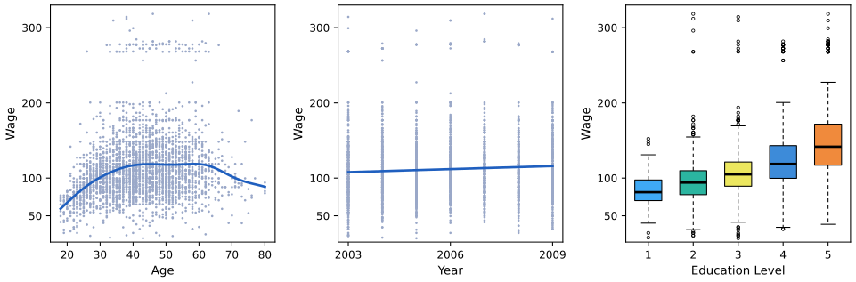
fig_1_1. Download: PDF · SVGThree features of the figure carry the chapter's message. The blue curve on the left is an estimate of the regression function \(f(\text{age})=\E(\text{wage}\given\text{age})\) of Result 1.1: it rises steeply up to about 40, stays near 118 thousand dollars between 45 and 60, and falls after that (its highest point is at age 58.5). But the points scatter widely around it, so age alone predicts an individual wage poorly: the irreducible error is large. Second, wage is related to all three inputs at once, so the best prediction combines them; Chapter 3 does this with linear regression and Chapter 7 with methods that allow the curved relation with age. Third, the band of points near 270 to 320 thousand dollars, at every age and year, is a separate group of very high earners that any model has to live with.
The numbers behind the description. The book says the average wage grows by “approximately $10,000” from 2003 to 2009. The yearly means are 106.2 in 2003 and 116.0 in 2009, a difference of 9.77 thousand dollars; the least-squares line in the centre panel has slope 1.350 per year, a fitted rise of \(6\times1.350=8.10\) thousand. Both are “about $10,000”, and both are small next to the standard deviation of wages, 41.7 thousand. The mean wage by education level is 84.1, 95.8, 107.8, 124.4 and 150.9 thousand dollars.
Filling the gap 1.2: the curve and the line in Figure 1.1 p. 2, “the blue line, which provides an estimate of the average wage”
The book does not say how the curve is computed. Here it is a local linear fit; the line in the centre is the least-squares line. How are they defined, and how are they related?
Derivation
The least-squares line. Choose \(a\) and \(b\) to minimise \(\RSS(a,b)=\sum_{i=1}^n(y_i-a-bx_i)^2\). Setting the two partial derivatives to zero gives the normal equations
\[ \sum_i(y_i-a-bx_i)=0,\qquad \sum_ix_i(y_i-a-bx_i)=0 . \]The first says \(a=\bar y-b\bar x\): the line passes through \((\bar x,\bar y)\). Substituting into the second and subtracting \(\bar x\) times the first,
\[ \sum_i(x_i-\bar x)\big(y_i-\bar y-b(x_i-\bar x)\big)=0\quad\Longrightarrow\quad \hat b=\frac{\sum_i(x_i-\bar x)(y_i-\bar y)}{\sum_i(x_i-\bar x)^2}. \]\(\RSS\) is a convex quadratic in \((a,b)\) (its second-derivative matrix is \(2\sum_i\begin{pmatrix}1&x_i\\x_i&x_i^2\end{pmatrix}\), positive definite unless all \(x_i\) are equal), so this stationary point is the minimum. On the Wage data with \(x=\) year, \(\hat b=1.3499\). Chapter 3 derives the same formula for many inputs.
The local linear fit. To estimate \(f(x_0)\), fit a line only to the points near \(x_0\), by weighted least squares with weights \(w_i=K\big((x_i-x_0)/h\big)\) that decay with distance. Here \(K(u)=e^{-u^2/2}\) (a Gaussian kernel) and \(h\), the bandwidth, is measured in years. Minimise \(\sum_iw_i\big(y_i-a-b(x_i-x_0)\big)^2\) and report \(\hat f(x_0)=\hat a\), the height of the local line at \(x_0\). With \(S_k=\sum_iw_i(x_i-x_0)^k\) and \(T_k=\sum_iw_i(x_i-x_0)^ky_i\), the weighted normal equations are \(aS_0+bS_1=T_0\) and \(aS_1+bS_2=T_1\), whose solution by Cramer's rule is
\[ \hat f(x_0)=\hat a=\frac{S_2T_0-S_1T_1}{S_0S_2-S_1^2}. \]Figure 1.1 uses \(h=5\) years.
The two extremes. As \(h\to\infty\) every weight tends to 1, the local fit at every \(x_0\) becomes the same ordinary least-squares line, and \(\hat f\) becomes that line. As \(h\to0\) only the points at (or nearest to) \(x_0\) count, and \(\hat f\) follows the noise. The bandwidth is the first example of the flexibility that Chapter 2 trades off against variance. ∎
Deeper: Statistical Learning: Theory and Methods, Section 6.1.1 (local linear regression, its equivalent kernel and its bias at the boundary) and Section 6.2 (choosing the bandwidth); Section 3.2 (least squares).
Filling the gap 1.3: how a boxplot is drawn Figures 1.1 and 1.2
The book's boxplots are drawn by R. The box runs from the lower hinge to the upper hinge with a thick line at the median; the whiskers reach the most extreme data points that lie within 1.5 box lengths of the box; points beyond the whiskers are drawn one by one. R's hinges are Tukey's: sort the data, split them at the median into a lower and an upper half (the median belongs to both halves when \(n\) is odd), and take the median of each half. Python's matplotlib instead uses the 25th and 75th percentiles computed by linear interpolation (R's quantile type 7, numpy's default). When do the two agree?
Result 1.2 (hinges and quartiles)
For sorted data \(x_{(1)}\le\dots\le x_{(n)}\), Tukey's lower hinge equals the type-7 first quartile whenever \(n\) is odd. When \(n\) is even they can differ, by at most half a gap \(x_{(k+1)}-x_{(k)}\) between neighbouring order statistics.
Proof
Both are values at a (possibly fractional) position in the sorted data, a fractional position \(k+t\) meaning \(x_{(k)}+t(x_{(k+1)}-x_{(k)})\), except that the hinge averages the two neighbours when it falls halfway. The type-7 first quartile sits at position \(1+(n-1)/4\). The lower half has \(\lfloor(n+1)/2\rfloor\) points, so the hinge sits at position \(m=\big(\lfloor(n+1)/2\rfloor+1\big)/2\). Check the four cases \(n=4j+r\):
- \(n=4j+1\): quartile at \(1+j\); \(m=(2j+1+1)/2=j+1\). Equal.
- \(n=4j+3\): quartile at \(1+(4j+2)/4=j+1.5\); \(m=(2j+2+1)/2=j+1.5\). Equal.
- \(n=4j\): quartile at \(j+0.75\); \(m=(2j+1)/2=j+0.5\). They differ by a quarter of the gap \(x_{(j+1)}-x_{(j)}\).
- \(n=4j+2\): quartile at \(j+1.25\); \(m=(2j+1+1)/2=j+1\). They differ by a quarter of the gap \(x_{(j+2)}-x_{(j+1)}\).
The upper hinge is symmetric. ∎
In Figure 1.1 the education groups have 268, 971, 650, 685 and 426 men. For the two odd groups the boxes of R and matplotlib coincide; for the three even groups they differ by up to 0.27 thousand dollars, invisible at the scale of the figure. The course's figure code computes the hinges as R does (box_stats), so its boxplots match the book's exactly.
See also (companion course): Statistical Methods for Modern Biology, Section 3.6.2 (boxplots, dot plots and violin plots in R).
1.1.2 Stock market data
pp. 2–4 The Smarket data cover the 1250 trading days of 2001 to 2005. For each day they give the percentage change of the S&P 500 index on that day (Today) and on each of the five previous days (Lag1 to Lag5), the trading volume, and whether the market went Up or Down. Predicting Up or Down is a classification problem: the output is a category, not a number.
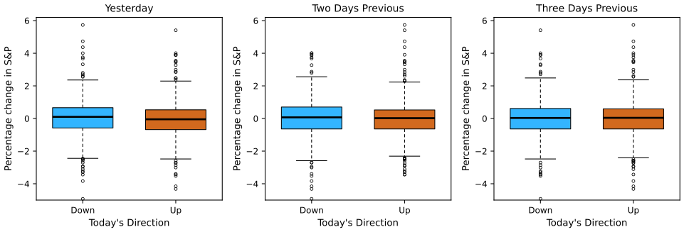
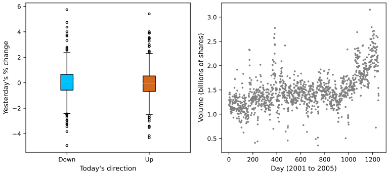
fig_1_2. Download: PDF · SVGHow different are the two boxes really? The mean of Lag1 is 0.0507 on Down days and −0.0397 on Up days; the Welch two-sample \(t\) statistic is 1.41 (two-sided \(p=0.16\)). For Lag2 and Lag3 the statistics are 0.85 and −0.22. The correlations between Today and the five lags are all between −0.04 and 0.00. If yesterday's move predicted today's, traders would exploit it until it no longer did, so this lack of pattern is what economics predicts. The only clearly non-zero correlation in the data is between Year and Volume (0.54): trading volume grew over the five years.
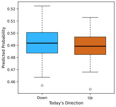
fig_1_3. Download: PDF · SVGFilling the gap 1.4: where the probabilities of Figure 1.3 come from p. 4, previewing Section 4.4.3
The chapter only names quadratic discriminant analysis. Here is the whole method, from Bayes' theorem.
Derivation
Let the output take classes \(k=1,\dots,K\) (here Down and Up), with prior probabilities \(\pi_k=\Pr(Y=k)\), and let \(f_k(x)\) be the density of \(X\) among units of class \(k\). Bayes' theorem gives the probability of class \(k\) for a unit with input \(x\):
\[ \Pr(Y=k\given X=x)=\frac{\pi_kf_k(x)}{\sum_{l=1}^K\pi_lf_l(x)}. \]QDA assumes each class is multivariate normal with its own mean \(\mu_k\) and its own covariance matrix \(\Sigma_k\):
\[ f_k(x)=\frac{1}{(2\pi)^{p/2}|\Sigma_k|^{1/2}}\exp\Big\{-\tfrac12(x-\mu_k)^\T\Sigma_k^{-1}(x-\mu_k)\Big\}. \]The factor \((2\pi)^{p/2}\) is common to all classes and cancels from the ratio, so the posterior probability is proportional to \(e^{\delta_k(x)}\), where
\[ \delta_k(x)=\log\pi_k-\tfrac12\log|\Sigma_k|-\tfrac12(x-\mu_k)^\T\Sigma_k^{-1}(x-\mu_k), \]and \(\Pr(Y=k\given X=x)=e^{\delta_k(x)}/\sum_le^{\delta_l(x)}\). Because \(\delta_k\) is a quadratic function of \(x\), the boundary \(\delta_{\rm Down}(x)=\delta_{\rm Up}(x)\) between the classes is a quadratic curve, hence the name. In practice the unknowns are replaced by estimates from the training days: \(\hat\pi_k\) is the proportion of class \(k\), \(\hat\mu_k\) the class mean vector, and \(\hat\Sigma_k\) the class sample covariance matrix (divisor \(n_k-1\)). On 2001–2004 there are 491 Down and 507 Up days, so \(\hat\pi_{\rm Down}=0.492\). If instead all classes share one covariance matrix the \(\log|\Sigma_k|\) and \(x^\T\Sigma^{-1}x\) terms are common to all classes and cancel, \(\delta_k\) becomes linear in \(x\), and the method is linear discriminant analysis (Chapter 4). ∎
Deeper: Statistical Learning: Theory and Methods, Section 4.3 (linear and quadratic discriminant analysis) and Section 4.3.1 (regularised discriminant analysis, between LDA and QDA).
Filling the gap 1.5: is 60% better than chance? p. 4, Figure 1.3
The book reports that the method predicts the direction correctly 60% of the time and calls it a hint of a weak trend. How much evidence is that?
Derivation
The right baseline is not 50%. In 2005 the market went Up on 141 of 252 days, so the trivial rule “always say Up” is right 55.95% of the time. QDA is right on 151 days, ten more.
Sampling variability. Treat the 252 test days as independent trials, each predicted correctly with probability \(\theta\). The number correct is binomial, and the observed proportion \(\hat\theta\) has standard error \(\sqrt{\hat\theta(1-\hat\theta)/252}=\sqrt{0.5992\times0.4008/252}=0.031\): three percentage points. A 95% confidence interval for \(\theta\) is roughly \(0.599\pm0.060\), which contains 0.5595.
A test. Under the null hypothesis that QDA is no better than always saying Up, \(\theta=0.5595\) and \(z=(0.5992-0.5595)/\sqrt{0.5595\times0.4405/252}=1.27\). The exact one-sided binomial \(p\)-value, \(\Pr(\text{Bin}(252,0.5595)\ge151)\), is 0.114. So the 60% is consistent with luck. (The independence assumption is itself questionable for daily returns, and the comparison ignores that the baseline was chosen after seeing 2005.) This is the sense in which the trend is only a hint; Chapter 4 returns to it, and Chapter 13 explains why trying many methods on the same test set makes the best one look better still.
Adding inputs does not help: QDA on all five lags and Volume is right on only 44.4% of the days of 2005, worse than always saying Up. ∎
1.1.3 Gene expression data
pp. 4–5 The NCI60 data hold 6830 gene expression measurements for each of 64 cancer cell lines. There is no output: the question is whether the cell lines fall into groups. With \(p=6830\) variables the data cannot be plotted directly, so the book first reduces each cell line to two numbers, \(Z_1\) and \(Z_2\), its first two principal component scores.
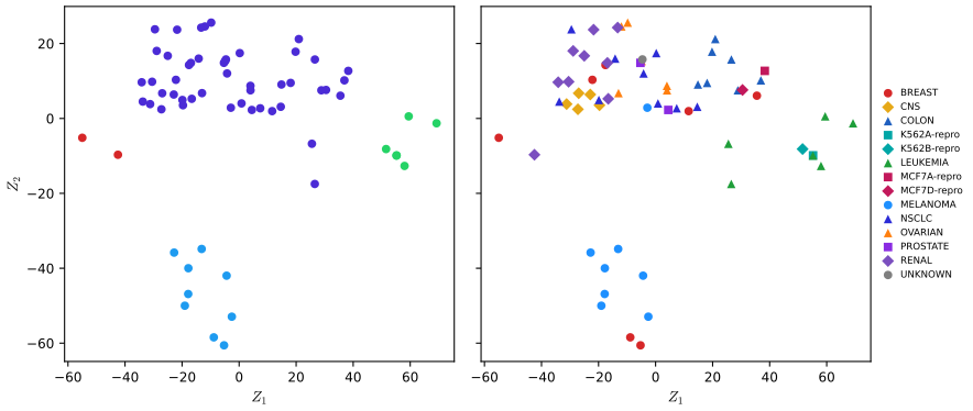
fig_1_4. Download: PDF · SVGDefinition 1.2 (principal components) p. 5; Section 12.2
Let the columns of the \(n\times p\) data matrix be centred to mean zero (and here also scaled to standard deviation one). The first principal component is the combination \(Z_1=\phi_{11}X_1+\dots+\phi_{p1}X_p\) with \(\sum_j\phi_{j1}^2=1\) whose values \(z_{i1}\) over the \(n\) units have the largest variance. The second, \(Z_2\), has the largest variance among unit-length combinations uncorrelated with \(Z_1\), and so on. The vectors \(\phi_1,\phi_2,\dots\) are the loadings, the numbers \(z_{im}\) the scores.
Result 1.3 (principal components from the covariance matrix)
Let \(\bS=\bX^\T\bX/(n-1)\) be the sample covariance matrix of the centred data. The first loading vector \(\phi_1\) is an eigenvector of \(\bS\) for its largest eigenvalue \(\lambda_1\), and the variance of the scores \(z_{i1}\) is \(\lambda_1\). In practice all components are obtained at once from the singular value decomposition \(\bX=\bU\bD\bV^\T\): the loadings are the columns of \(\bV\), the scores are \(\bU\bD\), and the proportion of variance explained by component \(m\) is \(d_m^2/\sum_kd_k^2\).
Proof
The scores are \(z_1=\bX\phi\), with sample variance \(\phi^\T\bX^\T\bX\phi/(n-1)=\phi^\T\bS\phi\) (their mean is zero because the columns are centred). Maximise \(\phi^\T\bS\phi\) subject to \(\phi^\T\phi=1\). With a Lagrange multiplier \(\lambda\), the gradient of \(\phi^\T\bS\phi-\lambda(\phi^\T\phi-1)\) is \(2\bS\phi-2\lambda\phi\), so at the maximum \(\bS\phi=\lambda\phi\): \(\phi\) is an eigenvector. Its objective value is then \(\phi^\T\bS\phi=\lambda\phi^\T\phi=\lambda\), so the best choice is the eigenvector of the largest eigenvalue. For the SVD, \(\bX^\T\bX=\bV\bD\bU^\T\bU\bD\bV^\T=\bV\bD^2\bV^\T\), so the columns of \(\bV\) are the eigenvectors of \(\bS\) with eigenvalues \(d_m^2/(n-1)\), and \(\bX\bV=\bU\bD\). The total variance is \(\tr\bS=\sum_md_m^2/(n-1)\), which gives the proportions. Each loading vector is defined only up to its sign: \(-\phi\) is as good as \(\phi\). ∎
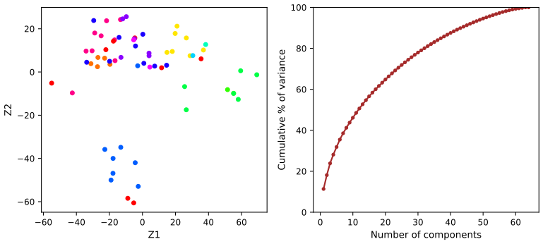
On the NCI60 data the first two components explain 11.4% and 6.8% of the total variance (the total is 6830, one per standardised gene). That is not much: Figure 1.4 is a useful but lossy picture. Because the 64 centred rows sum to zero, the centred matrix has rank at most 63, and indeed the 64th component has variance zero; with \(p\gg n\) there can never be more than \(n-1\) components with positive variance. Chapter 12 develops principal components and clustering fully, on these same data.
Filling the gap 1.6: what “four groups” means p. 5, “suggests at least four groups”
The book draws four groups in the left panel without saying how. A transparent way to find groups that the eye sees in a scatter plot is single-linkage clustering.
Derivation
Join two points by an edge whenever their distance is at most \(t\), and call the connected pieces of the resulting graph the groups at level \(t\). As \(t\) grows, groups merge; single-linkage hierarchical clustering records the order of the merges (two groups merge at the smallest distance between a point of one and a point of the other). To obtain four groups, stop merging when four are left: on the scores \((Z_1,Z_2)\) of NCI60 the last three merges happen at distances 16.7, 21.4 and 32.7, so any \(t\) from 16.7 up to (not including) 21.4 gives the same four groups, of 47, 9, 6 and 2 cell lines: the four groups of Figure 1.4. The bottom group is separated from the rest by a gap of 32.7, the widest of all, which is why it is the most convincing group in the picture. The book's caption is right to say “at least”: the number of groups is a choice, here of \(t\). Chapter 12 discusses complete and average linkage, which behave better than single linkage on most data, and how the choice of the number of clusters can be informed by the data. ∎
Deeper: Statistical Learning: Theory and Methods, Section 14.5.1 (principal components), Section 14.3.12 (hierarchical clustering) and Section 14.3.8 (clustering the same tumour microarray data).
See also (companion courses): Statistical Methods for Modern Biology, Section 7.6.3 (the singular value decomposition) and Section 5.6 (hierarchical clustering); Bayesian and Probabilistic Machine Learning, Section 12.1.1 (the maximum-variance view of principal components).
Note: “14 different types of cancer” p. 5, both editions
The NCI60 data carry 14 distinct labels, but they are not 14 types of cancer. Four labels mark repeat measurements of two cell lines kept as reproducibility controls (K562A-repro and K562B-repro, from a leukaemia line; MCF7A-repro and MCF7D-repro, from a breast cancer line), and one is UNKNOWN. The cell lines come from 9 tissues of origin: breast, central nervous system, colon, leukaemia, melanoma, non-small-cell lung, ovarian, prostate and renal. This matters for reading the right panel of Figure 1.4: the K562 repeats sit with the leukaemia lines, as they should.
1.2 A brief history of statistical learning
pp. 6–7 The methods of the book were invented over two centuries; what changed recently is the computing power and the free software that make them routine. The book's own timeline, with the original sources:
| When | Method | Original work | In this course |
|---|---|---|---|
| early 1800s | least squares, the first form of linear regression, used for astronomical orbits | Legendre (1805), Gauss (1809) | Chapter 3 |
| 1936 | linear discriminant analysis | Fisher (1936) | Chapter 4 |
| 1940s | logistic regression | Berkson (1944), among others | Chapter 4 |
| early 1970s | generalized linear models, a common frame for linear and logistic regression | Nelder and Wedderburn (1972) | Chapter 4 |
| mid 1980s | classification and regression trees | Breiman, Friedman, Olshen and Stone (1984) | Chapter 8 |
| late 1980s | generalized additive models | Hastie and Tibshirani (1986) | Chapter 7 |
| 1980s | neural networks trained by back-propagation | Rumelhart, Hinton and Williams (1986) | Chapter 10 |
| 1990s | support vector machines | Boser, Guyon and Vapnik (1992), Cortes and Vapnik (1995) | Chapter 9 |
Before about 1980 almost every method was linear, because fitting non-linear models was too expensive to compute; from the 1980s on, non-linear methods became practical. The R edition credits the free R system for spreading these methods beyond statisticians and computer scientists; the Python edition says the same of Python.
1.3 This book, and who should read it
pp. 6–9 The book is the introductory companion of The Elements of Statistical Learning (Hastie, Tibshirani and Friedman 2001, 2009), written for readers who will use the methods rather than develop them: students and practitioners in business, biology, the social sciences and elsewhere with one course in statistics behind them. It rests on four premises: the methods are useful far beyond statistics; they should not be used as black boxes, because no method is best for every problem; one needs to know what each part of a method does without being able to build it, so the book keeps fitting algorithms, theory and matrix algebra to a minimum; and the reader wants to apply the methods, so every chapter ends with computer labs.
The two editions differ only in that last point. The R edition (2013, second edition 2021) has labs in R; the Python edition (2023) rewrote every lab in Python, using standard packages plus a helper package written by the authors. This course follows both: the notes cover the shared text once, and each lab is shown in both languages. Its Python code uses only general-purpose packages (pandas, numpy, statsmodels, scikit-learn, matplotlib), so it runs without the helper package; its R code uses base R and the packages named by the R edition. For readers who want the proofs that the book leaves out, the graduate course Statistical Learning: Theory and Methods is linked throughout.
1.4 Notation and simple matrix algebra
pp. 9–12 The book uses the notation of the graduate book, with \(n\) (not \(N\)) for the number of observations.
Definition 1.3 (the book's notation) pp. 9–11, (1.1)
Sizes and indices. \(n\) is the number of observations, indexed by \(i=1,\dots,n\); \(p\) is the number of variables, indexed by \(j=1,\dots,p\). \(x_{ij}\) is the value of variable \(j\) for observation \(i\), and \(\bX\) is the \(n\times p\) matrix with \((i,j)\) entry \(x_{ij}\), a spreadsheet with one row per observation and one column per variable.
Rows and columns. The \(i\)th row, written as a column vector, is \(x_i=(x_{i1},\dots,x_{ip})^\T\in\R^p\) (1.1); the \(j\)th column is \(\bx_j=(x_{1j},\dots,x_{nj})^\T\in\R^n\). So \(\bX=(\bx_1\ \bx_2\ \cdots\ \bx_p)\), and \(\bX\) stacks the rows \(x_1^\T,\dots,x_n^\T\). The outputs form \(\by=(y_1,\dots,y_n)^\T\), and the data are the pairs \((x_1,y_1),\dots,(x_n,y_n)\).
Typography. A vector of length \(n\) is bold lower case (\(\ba\)); any other vector, and any scalar, is plain lower case (\(a\)); a matrix is bold upper case (\(\bA\)); a random variable is plain upper case (\(A\)). \(a\in\R\), \(a\in\R^k\) and \(\bA\in\R^{r\times s}\) state that an object is a scalar, a vector of length \(k\), or an \(r\times s\) matrix. All vectors are columns; \(^\T\) is the transpose, which turns rows into columns.
Example: the Wage data. \(n=3000\). The book says \(p=11\), counting every column of the data set; but two of the eleven columns are the output, wage, and its logarithm, logwage, so as inputs for predicting wage there are 9 variables (year, age, marital status, race, education, region, job class, health, health insurance), and region takes a single value in these data (all 3000 men are from the Middle Atlantic region). \(\bx_1\) is the column of 3000 years, and \(x_1\) the 11 values recorded for the first man.
Definition 1.4 (matrix product) pp. 11–12
If \(\bA\in\R^{r\times d}\) and \(\bB\in\R^{d\times s}\), the product \(\bA\bB\in\R^{r\times s}\) has entries
\[ (\bA\bB)_{ij}=\sum_{k=1}^da_{ik}b_{kj}, \]the sum of the products of row \(i\) of \(\bA\) with column \(j\) of \(\bB\). It exists only when the number of columns of \(\bA\) equals the number of rows of \(\bB\). The book's example:
\[ \begin{pmatrix}1&2\\3&4\end{pmatrix}\begin{pmatrix}5&6\\7&8\end{pmatrix}=\begin{pmatrix}1\cdot5+2\cdot7&1\cdot6+2\cdot8\\3\cdot5+4\cdot7&3\cdot6+4\cdot8\end{pmatrix}=\begin{pmatrix}19&22\\43&50\end{pmatrix}. \]Result 1.4 (rules of matrix algebra used in the book)
For matrices of compatible sizes:
(a) \((\bA\bB)\bC=\bA(\bB\bC)\) and \(\bA(\bB+\bC)=\bA\bB+\bA\bC\), but in general \(\bA\bB\ne\bB\bA\): in the example, \(\bB\bA=\begin{pmatrix}23&34\\31&46\end{pmatrix}\).
(b) \((\bA\bB)^\T=\bB^\T\bA^\T\).
(c) For the data matrix, \(\bX^\T\bX=\sum_{i=1}^nx_ix_i^\T\) (a \(p\times p\) matrix) and \(\bX^\T\by=\sum_{i=1}^nx_iy_i\); the \((j,k)\) entry of \(\bX^\T\bX\) is \(\bx_j^\T\bx_k=\sum_ix_{ij}x_{ik}\).
(d) If the columns of \(\bX\) are centred, \(\bX^\T\bX/(n-1)\) is the sample covariance matrix of the \(p\) variables.
Proof
(a) \(\big((\bA\bB)\bC\big)_{ij}=\sum_l\sum_ka_{ik}b_{kl}c_{lj}=\big(\bA(\bB\bC)\big)_{ij}\), by exchanging two finite sums; distributivity is the same computation with a sum inside. The example shows non-commutativity.
(b) \(\big((\bA\bB)^\T\big)_{ij}=(\bA\bB)_{ji}=\sum_ka_{jk}b_{ki}=\sum_k(\bB^\T)_{ik}(\bA^\T)_{kj}=(\bB^\T\bA^\T)_{ij}\).
(c) \((\bX^\T\bX)_{jk}=\sum_i(\bX^\T)_{ji}x_{ik}=\sum_ix_{ij}x_{ik}\), which is also the \((j,k)\) entry of \(\sum_ix_ix_i^\T\), since \((x_ix_i^\T)_{jk}=x_{ij}x_{ik}\). The same computation gives \(\bX^\T\by\).
(d) With centred columns, \(\sum_ix_{ij}x_{ik}/(n-1)\) is the sample covariance of variables \(j\) and \(k\) (the sample variance when \(j=k\)). ∎
Part (c) is how most of the book's matrix formulas should be read: \(\bX^\T\bX\) collects all the sums of squares and cross-products of the variables, and it is the matrix that appears in least squares (Chapter 3) and principal components (Result 1.3).
Deeper: Statistical Learning: Theory and Methods, Section 1.1.2 (the same notation, with \(N\) for \(n\) and \(G\) for a qualitative output) and Section 2.2 (variable types and terminology).
1.5 Organization of this book
pp. 12–13 The plan of the book, which is the plan of this course:
| Chapter | Topic | Data of Chapter 1 used |
|---|---|---|
| 2 | Statistical learning: \(f\), prediction and inference, the bias–variance trade-off, K-nearest neighbours | |
| 3 | Linear regression | |
| 4 | Classification: logistic regression, LDA, QDA, naive Bayes, K-nearest neighbours, Poisson regression | Smarket |
| 5 | Resampling methods: cross-validation and the bootstrap | |
| 6 | Linear model selection and regularization: subset selection, ridge, lasso, principal components regression, partial least squares | |
| 7 | Moving beyond linearity: polynomials, step functions, splines, local regression, generalized additive models | Wage |
| 8 | Tree-based methods: bagging, random forests, boosting, Bayesian additive regression trees | |
| 9 | Support vector machines | |
| 10 | Deep learning | |
| 11 | Survival analysis and censored data | |
| 12 | Unsupervised learning: principal components, K-means and hierarchical clustering | NCI60 |
| 13 | Multiple testing |
Each chapter ends with labs (in R or in Python depending on the edition, in both here) and exercises; sections and exercises marked with a special symbol in the book are more demanding and can be skipped.
1.6 Data sets used in labs and exercises
pp. 13–14, Table 1.1 The book's data sets come with the R package ISLR2 (R edition) and the Python package of the Python edition; USArrests is part of base R. The book's website also offers them as CSV files, which this course reads in Python. The sizes, computed from the data (for the data stored only in the R package, in R):
| Name | Content | \(n\) | columns |
|---|---|---|---|
| Auto | fuel economy, horsepower and other features of cars | 392 | 9 |
| Bikeshare | hourly use of a bike-sharing scheme in Washington, DC | 8645 | 15 |
| Boston | housing values and other features of Boston census tracts | 506 | 13 |
| BrainCancer | survival times of brain cancer patients | 88 | 8 |
| Caravan | people offered caravan insurance | 5822 | 86 |
| Carseats | child car seat sales in 400 stores | 400 | 11 |
| College | applications, tuition and other features of US colleges | 777 | 18 |
| Credit | credit card balances of customers | 400 | 11 |
| Default | credit card default records | 10000 | 4 |
| Fund | monthly returns of 2000 hedge fund managers | 50 | 2000 |
| Hitters | baseball players' records and salaries | 322 | 20 |
| Khan | gene expression of four types of small round blue cell tumour | 63 + 20 | 2308 |
| NCI60 | gene expression of 64 cancer cell lines | 64 | 6830 |
| NYSE | returns, volatility and volume of the New York Stock Exchange, 1962–1986 | 6051 | 6 |
| OJ | purchases of two brands of orange juice | 1070 | 18 |
| Portfolio | returns of two assets | 100 | 2 |
| Publication | time to publication of 244 clinical trials | 244 | 9 |
| Smarket | daily S&P 500 returns, 2001–2005 | 1250 | 9 |
| USArrests | arrests per 100,000 residents in the 50 US states (base R) | 50 | 4 |
| Wage | wages and other features of men in the Middle Atlantic region | 3000 | 11 |
| Weekly | weekly S&P 500 returns, 1990–2010 (21 years) | 1089 | 9 |
Auto: the CSV file on the book's website has 397 rows, five of them with horsepower missing (coded “?”); the R package drops them, leaving 392. Khan comes split into 63 training and 20 test samples. Columns include the output where there is one.
Correction to Table 1.1 of the R edition: the Credit data James et al. (2021), p. 14
Table 1.1 of the R edition describes Credit as “credit card debt for 10,000 customers”. The data set has 400 customers (it is the Default data that has 10,000 rows). The Python edition's Table 1.1 gives the correct 400.
1.7 Book website
p. 14 The book's website, www.statlearning.com, has the R and Python packages, the data sets, the labs and further resources. All figures of the book are new except three taken from the graduate book (Figures 6.7, 8.3 and 12.14); in the Python edition Figure 13.10 differs from the R edition because of the software that produced it.
1.8 Lab: a first session in R and Python
The book has no lab in Chapter 1; the labs start in Chapter 2 with an introduction to the language of each edition (Section 2.3). This lab is a short tour of both languages on the three data sets of this chapter, so that the side-by-side format of the course is familiar before the real labs start. It loads each data set, summarises it, draws a first plot, and recomputes the numbers behind Figures 1.3 and 1.4.
The files. code/ch01_lab.R (run with Rscript ch01_lab.R from the code folder; it needs the CRAN packages ISLR2 and MASS) and code/ch01_lab.py (run with python3 ch01_lab.py; it needs numpy, pandas, matplotlib, statsmodels and scikit-learn). The code below is copied from these files, R on the left and Python on the right. The R script reads the data from the ISLR2 package; the Python script reads the book's CSV files with the helper isl_data of common.py. Every number below is the same in the two languages unless an orange note says otherwise.
1.8.1 Vectors and matrices
Vectors are created with c() in R and as numpy arrays in Python. Arithmetic is elementwise in both.
R
x <- c(1, 6, 2)
y <- c(1, 4, 3)
length(x)
x + y                       # elementwise
x[1]                        # R counts from 1
Python
x = np.array([1, 6, 2])
y = np.array([1, 4, 3])
print(len(x))
print(x + y)                    # elementwise
print(x[0])                     # Python counts from 0
Output (both): 3, 2 10 5, 1
x[1] is the first element; Python numbers them from 0, so the first element is x[0]. The book's \(x_{ij}\) is X[i, j] in R and X[i-1, j-1] in Python.The matrix product of Definition 1.4:
R
A <- matrix(c(1, 2, 3, 4), nrow = 2, byrow = TRUE)
B <- matrix(c(5, 6, 7, 8), nrow = 2, byrow = TRUE)
A %*% B                     # matrix product: 19 22 / 43 50
A * B                       # elementwise product: 5 12 / 21 32
t(A)                        # transpose
A[2, 1]                     # row 2, column 1: the entry a_21 = 3
Python
A = np.array([[1, 2], [3, 4]])
B = np.array([[5, 6], [7, 8]])
print(A @ B)                    # matrix product: 19 22 / 43 50
print(A * B)                    # elementwise product: 5 12 / 21 32
print(A.T)                      # transpose
print(A[1, 0])                  # row 2, column 1: the entry a_21 = 3
[,1] [,2] A %*% B / A @ B A * B (both) [1,] 19 22 5 12 [2,] 43 50 21 32 A[2, 1] / A[1, 0]: 3
* multiplies entry by entry (A * B is 5, 12, 21, 32). The matrix product is %*% in R and @ in Python. R's matrix() fills by column unless byrow = TRUE; numpy arrays are written row by row.1.8.2 The Wage data
R
dim(Wage)                   # n = 3000 rows, 11 columns
names(Wage)
head(Wage[, c("year", "age", "education", "wage")], 3)
Python
Wage = isl_data("Wage")
print(Wage.shape)               # n = 3000 rows, 11 columns
print(list(Wage.columns))
print(Wage[["year", "age", "education", "wage"]].head(3))
Output: 3000 rows and 11 columns; the first man is 18 years old, has no high-school diploma and earned 75.04 thousand dollars in 2006.
R
summary(Wage$wage)
table(Wage$education)
round(tapply(Wage$wage, Wage$education, mean), 2)
Python
print(Wage["wage"].describe().round(2))
print(Wage["education"].value_counts().sort_index())
print(Wage.groupby("education")["wage"].mean().round(2))
Min. 1st Qu. Median Mean 3rd Qu. Max. (R summary; describe() adds count 3000 and std 41.73) 20.09 85.38 104.92 111.70 128.68 318.34 education: 1. < HS Grad 268 2. HS Grad 971 3. Some College 650 4. College Grad 685 5. Advanced Degree 426 mean wage: 84.10 95.78 107.76 124.43 150.92
summary() gives the minimum, quartiles, median, mean and maximum; pandas' describe() gives the count, mean, standard deviation, minimum, quartiles and maximum. The quartiles agree (both use R's default type 7). The standard deviation of pandas uses the divisor \(n-1\), like R's sd(); numpy's np.std uses \(n\) unless told ddof=1.The least-squares line of wage on year (the centre panel of Figure 1.1, and Filling the gap 1.2):
R
fit_year <- lm(wage ~ year, data = Wage)
coef(fit_year)
6 * coef(fit_year)["year"]  # fitted change from 2003 to 2009, in thousands of dollars
Python
fit_year = smf.ols("wage ~ year", data=Wage).fit()
print(fit_year.params)
print(6 * fit_year.params["year"])  # fitted change from 2003 to 2009, in thousands of dollars
(Intercept) year -2595.861553 1.349874 fitted change 2003 to 2009: 8.099244
Both languages use the same model formula, wage ~ year: R's lm and the formula interface of statsmodels read it the same way.
R
png(file.path(out_dir, "lab-r-wage.png"), width = 900, height = 420, res = 110)
par(mfrow = c(1, 2), mar = c(4.2, 4.2, 1, 1))
plot(Wage$age, Wage$wage, pch = 20, cex = 0.4, col = "steelblue",
     xlab = "Age", ylab = "Wage")
smooth <- lowess(Wage$age, Wage$wage, f = 0.3)
lines(smooth, col = "darkblue", lwd = 2)
boxplot(wage ~ as.integer(education), data = Wage, col = "lightblue",
        xlab = "Education level", ylab = "Wage")
invisible(dev.off())
Python
fig, ax = plt.subplots(1, 2, figsize=(8.2, 3.8))
ax[0].scatter(Wage["age"], Wage["wage"], s=3, color="steelblue")
smooth = lowess(Wage["wage"], Wage["age"], frac=0.3, it=3, delta=0.01 * np.ptp(Wage["age"]))
ax[0].plot(smooth[:, 0], smooth[:, 1], color="darkblue", lw=2)
ax[0].set_xlabel("Age")
ax[0].set_ylabel("Wage")
groups = [g["wage"].to_numpy() for _, g in Wage.groupby("education")]
ax[1].boxplot(groups, tick_labels=[1, 2, 3, 4, 5], patch_artist=True,
              boxprops=dict(facecolor="lightblue"), flierprops=dict(markersize=3))
ax[1].set_xlabel("Education level")
ax[1].set_ylabel("Wage")
fig.tight_layout()
save(fig, "lab-py-wage")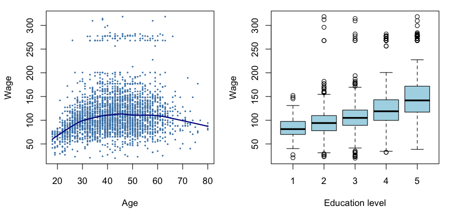
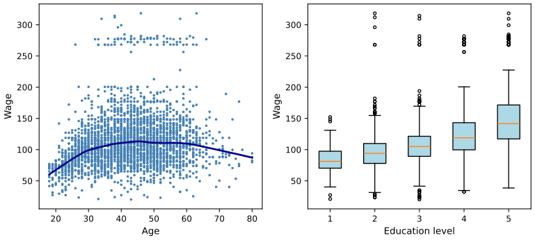
lowess and statsmodels' lowess give the same curve to 8 decimals. Download: R (PNG) · Python (SVG)lowess matches R's only when given R's defaults explicitly: it=3 robustness steps and delta equal to 1% of the range of \(x\) (statsmodels' own default is delta=0); note also that it takes \(y\) first and \(x\) second. The boxes of matplotlib use type-7 quartiles, R's use Tukey's hinges; by Result 1.2 they coincide for the groups with an odd number of men (971 and 685) and differ slightly for the others.1.8.3 The Smarket data
R
dim(Smarket)
table(Smarket$Direction)
round(cor(Smarket[, -9]), 2)
Python
Smarket = isl_data("Smarket")
print(Smarket.shape)
print(Smarket["Direction"].value_counts().sort_index())
print(Smarket.drop(columns="Direction").corr().round(2))
1250 rows, 9 columns; Down 602, Up 648
Year Lag1 Lag2 Lag3 Lag4 Lag5 Volume Today
Year 1.00 0.03 0.03 0.03 0.04 0.03 0.54 0.03
Lag1 0.03 1.00 -0.03 -0.01 0.00 -0.01 0.04 -0.03
...
Volume 0.54 0.04 -0.04 -0.04 -0.05 -0.02 1.00 0.01
Today 0.03 -0.03 -0.01 0.00 -0.01 -0.03 0.01 1.00
Correlations need numeric columns, so the qualitative Direction is dropped first: column 9 in R (Smarket[, -9], a negative index removes), by name in Python.
R
aggregate(cbind(Lag1, Lag2, Lag3) ~ Direction, data = Smarket, FUN = mean)
t.test(Lag1 ~ Direction, data = Smarket)$statistic
Python
print(Smarket.groupby("Direction")[["Lag1", "Lag2", "Lag3"]].mean())
down = Smarket.loc[Smarket["Direction"] == "Down", "Lag1"]
up = Smarket.loc[Smarket["Direction"] == "Up", "Lag1"]
print(stats.ttest_ind(down, up, equal_var=False).statistic)
Direction Lag1 Lag2 Lag3 Down 0.050686 0.032297 -0.005525 Up -0.039691 -0.022444 0.008443 Welch t (Lag1, Down minus Up): 1.40516
t.test(Lag1 ~ Direction) uses Welch's unequal-variance test by default and subtracts the second level (Up) from the first (Down). scipy's ttest_ind assumes equal variances unless equal_var=False, and subtracts its second argument from its first; the order of the arguments fixes the sign.R
png(file.path(out_dir, "lab-r-smarket.png"), width = 900, height = 420, res = 110)
par(mfrow = c(1, 2), mar = c(4.2, 4.2, 1, 1))
boxplot(Lag1 ~ Direction, data = Smarket, col = c("deepskyblue", "chocolate"),
        xlab = "Today's direction", ylab = "Yesterday's % change")
plot(Smarket$Volume, pch = 20, cex = 0.4, col = "grey40",
     xlab = "Day (2001 to 2005)", ylab = "Volume (billions of shares)")
invisible(dev.off())
Python
fig, ax = plt.subplots(1, 2, figsize=(8.2, 3.8))
bp = ax[0].boxplot([down, up], tick_labels=["Down", "Up"], patch_artist=True, flierprops=dict(markersize=3))
for patch, colour in zip(bp["boxes"], ["deepskyblue", "chocolate"]):
    patch.set_facecolor(colour)
ax[0].set_xlabel("Today's direction")
ax[0].set_ylabel("Yesterday's % change")
ax[1].scatter(np.arange(1, len(Smarket) + 1), Smarket["Volume"], s=3, color="grey")
ax[1].set_xlabel("Day (2001 to 2005)")
ax[1].set_ylabel("Volume (billions of shares)")
fig.tight_layout()
save(fig, "lab-py-smarket")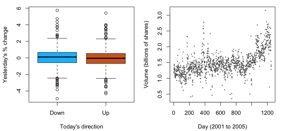
Finally the model behind Figure 1.3: QDA with Lag1 and Lag2, trained on 2001–2004 and tested on 2005 (Filling the gap 1.4).
R
train <- Smarket$Year < 2005
qda_fit <- qda(Direction ~ Lag1 + Lag2, data = Smarket, subset = train)
qda_pred <- predict(qda_fit, Smarket[!train, ])
p_down <- qda_pred$posterior[, "Down"]
table(predicted = qda_pred$class, actual = Smarket$Direction[!train])
mean(qda_pred$class == Smarket$Direction[!train])
Python
train = (Smarket["Year"] < 2005).to_numpy()
X_train, y_train = Smarket.loc[train, ["Lag1", "Lag2"]], Smarket.loc[train, "Direction"]
X_test, y_test = Smarket.loc[~train, ["Lag1", "Lag2"]], Smarket.loc[~train, "Direction"]
qda_fit = QuadraticDiscriminantAnalysis().fit(X_train, y_train)
qda_class = qda_fit.predict(X_test)
p_down = qda_fit.predict_proba(X_test)[:, list(qda_fit.classes_).index("Down")]
print(pd.crosstab(pd.Series(qda_class, name="predicted"), pd.Series(y_test.to_numpy(), name="actual")))
print(np.mean(qda_class == y_test.to_numpy()))
actual
predicted Down Up
Down 30 20
Up 81 121
accuracy: 0.5992063
The two implementations agree to 12 decimals on all 252 probabilities: both estimate the class covariance matrices with divisor \(n_k-1\) and the priors by the class proportions. QDA calls only 50 of the 252 days Down, so its 60% comes mostly from the Up days, which is why it beats always saying Up by only ten days (Filling the gap 1.5).
qda takes a model formula and a subset; scikit-learn takes the input matrix and the output vector separately, and its predict_proba orders the columns by classes_ (alphabetically, Down then Up), so the column of Down is looked up rather than assumed.1.8.4 The NCI60 data
R
nci_labs <- NCI60$labs
nci_data <- NCI60$data
dim(nci_data)               # 64 cell lines, 6830 genes
table(nci_labs)
Python
nci_data, nci_labs = load_nci60()
print(nci_data.shape)           # 64 cell lines, 6830 genes
print(pd.Series(nci_labs).value_counts().sort_index())
Output: 64 rows and 6830 columns; the label counts are BREAST 7, CNS 5, COLON 7, K562A-repro 1, K562B-repro 1, LEUKEMIA 6, MCF7A-repro 1, MCF7D-repro 1, MELANOMA 8, NSCLC 9, OVARIAN 6, PROSTATE 2, RENAL 9, UNKNOWN 1 (see the note on the labels).
load_nci60() reads a copy exported once from ISLR2, so both languages analyse identical numbers.Principal components of the standardised data (Result 1.3): R's prcomp does the centring, scaling and singular value decomposition; in Python they are three explicit lines.
R
pr_out <- prcomp(nci_data, scale = TRUE)
pve <- pr_out$sdev^2 / sum(pr_out$sdev^2)
round(pve[1:3], 4)
round(head(pr_out$x[, 1:2], 3), 3)
Python
Z = (nci_data - nci_data.mean(axis=0)) / nci_data.std(axis=0, ddof=1)   # as prcomp(scale = TRUE)
U, d, Vt = np.linalg.svd(Z, full_matrices=False)
scores = U * d                  # principal component scores, one row per cell line
pve = d ** 2 / np.sum(d ** 2)
print(pve[:3].round(4))
print(scores[:3, :2].round(3))
proportion of variance: 0.1136 0.0676 0.0575 scores of the first three cell lines: Z1 Z2 -19.682 3.528 -22.908 6.391 -27.241 2.446
prcomp(scale = TRUE) divides each gene by its standard deviation with divisor \(n-1\); scikit-learn's StandardScaler uses divisor \(n\), which multiplies every score by \(\sqrt{64/63}=1.0079\). The proportions of variance are unaffected.R
png(file.path(out_dir, "lab-r-nci60.png"), width = 900, height = 420, res = 110)
par(mfrow = c(1, 2), mar = c(4.2, 4.2, 1, 1))
cols <- rainbow(length(unique(nci_labs)))[as.integer(factor(nci_labs))]
plot(pr_out$x[, 1:2], col = cols, pch = 19, xlab = "Z1", ylab = "Z2")
plot(100 * cumsum(pve), type = "o", pch = 20, col = "brown3", ylim = c(0, 100),
     xlab = "Number of components", ylab = "Cumulative % of variance")
invisible(dev.off())
Python
fig, ax = plt.subplots(1, 2, figsize=(8.2, 3.8))
codes, names = pd.factorize(pd.Series(nci_labs), sort=True)
ax[0].scatter(scores[:, 0], scores[:, 1], c=codes, cmap="hsv", s=18)
ax[0].set_xlabel("Z1")
ax[0].set_ylabel("Z2")
ax[1].plot(np.arange(1, len(pve) + 1), 100 * np.cumsum(pve), "o-", color="brown", ms=3)
ax[1].set_ylim(0, 100)
ax[1].set_xlabel("Number of components")
ax[1].set_ylabel("Cumulative % of variance")
fig.tight_layout()
save(fig, "lab-py-nci60")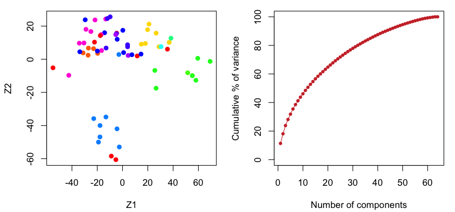
1.8.5 Where R and Python differ
Everything in this lab is deterministic, and every number agrees between the two languages, to the printed precision and in fact to at least 8 decimals. The differences are in conventions, which are worth learning once:
| Topic | R | Python |
|---|---|---|
| first element | x[1] | x[0] |
| matrix product | A %*% B | A @ B |
| standard deviation | sd(), divisor \(n-1\) | pandas .std() divisor \(n-1\); numpy np.std divisor \(n\) unless ddof=1 |
| categories | factors with levels | strings or pandas categoricals |
| boxplot box | Tukey's hinges | type-7 quartiles (equal when \(n\) is odd) |
| two-sample t test | Welch by default | scipy: pooled by default, equal_var=False for Welch |
| lowess | defaults iter = 3, delta = 1% of range | statsmodels: it=3, delta=0; arguments \(y\) then \(x\) |
| model formulas | built in (lm, qda) | statsmodels formulas; scikit-learn takes arrays |
| PCA scaling | prcomp(scale = TRUE), divisor \(n-1\) | StandardScaler, divisor \(n\) |
Exercises
Chapter 1 of the book has no exercises (they start in Chapter 2). Five short practice problems on this chapter follow, with solutions; the applied ones are solved in both languages.
Practice 1.1. For each problem, say whether it is supervised or unsupervised, and if supervised whether it is regression or classification; give \(n\) and \(p\). (a) Predicting a man's wage from the other columns of the Wage data. (b) Predicting whether a customer in the Default data will default. (c) Grouping the 50 states of USArrests by their crime statistics.
Solution
(a) Supervised regression; \(n=3000\), and \(p=9\) inputs (logwage must be left out, since it is a function of the output). (b) Supervised classification; \(n=10000\), \(p=3\) inputs (student, balance, income), output default. (c) Unsupervised (clustering); \(n=50\), \(p=4\).
Practice 1.2. Let \(\bA\) be \(3\times2\) and \(\bB\) be \(2\times4\). Which of \(\bA\bB\), \(\bB\bA\), \(\bA^\T\bA\), \(\bB\bB^\T\) exist, and what are their sizes? Show that \(\bA^\T\bA\) is always symmetric.
Solution
\(\bA\bB\) is \(3\times4\); \(\bB\bA\) does not exist (\(\bB\) has 4 columns, \(\bA\) has 3 rows); \(\bA^\T\bA\) is \(2\times2\); \(\bB\bB^\T\) is \(2\times2\). By Result 1.4(b), \((\bA^\T\bA)^\T=\bA^\T(\bA^\T)^\T=\bA^\T\bA\).
Practice 1.3. In the Wage data, compute the mean wage of men in industrial and in information jobs, and the slope of the least-squares line of wage on age. Is the line a good summary of the left panel of Figure 1.1?
Solution
R
tapply(Wage$wage, Wage$jobclass, mean)
coef(lm(wage ~ age, data = Wage))
Python
Wage.groupby("jobclass")["wage"].mean()
smf.ols("wage ~ age", data=Wage).fit().params
Industrial 103.32, information 120.59 thousand dollars; intercept 81.70 and slope 0.707 thousand dollars per year of age. The line says wages keep rising by about $700 a year at every age, which misses both the steep rise before 40 and the fall after 60 that the local linear fit shows (demo, preset 5): a straight line is too rigid here, the problem Chapter 7 addresses.
Practice 1.4. For each year of the Smarket data, compute the proportion of Up days. What accuracy does “always predict Up” have on 2005, and what does this say about Figure 1.3?
Solution
R
tapply(Smarket$Direction == "Up", Smarket$Year, mean)Python
(Smarket["Direction"] == "Up").groupby(Smarket["Year"]).mean()2001: 0.4835, 2002: 0.4444, 2003: 0.5476, 2004: 0.5556, 2005: 0.5595. Always saying Up is right 55.95% of the time in 2005, so QDA's 59.92% is four points above the obvious baseline, not ten points above a coin toss; with a standard error of three points this is weak evidence (Filling the gap 1.5). Note also that the best constant rule would have been “always Down” in 2001 and 2002: the baseline itself changes from year to year.
Practice 1.5. For the data 1, 2, 3, 4 compute Tukey's hinges and the type-7 quartiles, and check your answer with
fivenumandquantilein R, andnp.percentilein Python. Then show that principal component scores have mean zero and that the scores of two different components are uncorrelated.Solution
\(n=4\): the lower half is \(\{1,2\}\), so the lower hinge is 1.5 and the upper hinge 3.5; the type-7 quartiles sit at positions \(1+3/4=1.75\) and \(3.25\), giving 1.75 and 3.25. This is the case \(n=4j\) of Result 1.2, a difference of a quarter of a gap.
R
fivenum(c(1, 2, 3, 4))      # 1.0 1.5 2.5 3.5 4.0
quantile(c(1, 2, 3, 4))     # 1.00 1.75 2.50 3.25 4.00
Python
np.percentile([1, 2, 3, 4], [25, 75]) # 1.75 3.25For the scores: \(\bone^\T\bX\phi_m=0\) because each column of the centred \(\bX\) sums to zero, so every score vector has mean zero. With the SVD, the score vectors are the columns of \(\bU\bD\), and \((\bU\bD)^\T\bU\bD=\bD\bU^\T\bU\bD=\bD^2\) is diagonal, so the sample covariance of scores \(m\ne l\) is \(0\).
Demonstrations for this chapter
Each demonstration runs in the browser on the book's own data and links back to these notes. The ▶ Demo boxes above open them already set to the case under discussion.
| Demonstration | What you can see | Sections and results |
|---|---|---|
| Exploring the Wage data | Wage against age with a local linear fit and a bandwidth slider, against year with the least-squares line, and by education with R-style boxplots, for all men or one job class. Presets: 1 Figure 1.1, left; 2 centre; 3 right; 4 \(h=1\); 5 \(h=30\) against the line; 6 information jobs. | 1.1.1, 1.8.2; Filling the gap 1.2, 1.3 |
| Up and down days on the stock market | Boxplots of any lag, the volume or today's return on Up and Down days with Welch's t; QDA on any set of inputs trained on 2001–2004, its probabilities for 2005, a threshold, the confusion table and the accuracy against always saying Up. Presets: 1–3 Figure 1.2; 4 Figure 1.3; 5 six inputs; 6 a leaky predictor. | 1.1.2, 1.8.3; Filling the gap 1.4, 1.5 |
The code: code/ch01_introduction.py makes every figure of the chapter and the demonstrations' data; code/ch01_lab.R and code/ch01_lab.py are the lab (see the code index).
References
- James, G., Witten, D., Hastie, T. and Tibshirani, R. (2021). An Introduction to Statistical Learning with Applications in R, 2nd edition. Springer, New York. Chapter 1, pp. 1–14. www.statlearning.com.
- James, G., Witten, D., Hastie, T., Tibshirani, R. and Taylor, J. (2023). An Introduction to Statistical Learning with Applications in Python. Springer, Cham. Chapter 1, pp. 1–13.
- Hastie, T., Tibshirani, R. and Friedman, J. (2009). The Elements of Statistical Learning: Data Mining, Inference, and Prediction, 2nd edition. Springer, New York.
- Berkson, J. (1944). Application of the logistic function to bio-assay. Journal of the American Statistical Association, 39(227), 357–365.
- Boser, B. E., Guyon, I. M. and Vapnik, V. N. (1992). A training algorithm for optimal margin classifiers. Proceedings of the Fifth Annual Workshop on Computational Learning Theory, 144–152.
- Breiman, L., Friedman, J., Olshen, R. and Stone, C. (1984). Classification and Regression Trees. Wadsworth, Belmont, CA.
- Cleveland, W. S. (1979). Robust locally weighted regression and smoothing scatterplots. Journal of the American Statistical Association, 74(368), 829–836.
- Cortes, C. and Vapnik, V. (1995). Support-vector networks. Machine Learning, 20(3), 273–297.
- Fisher, R. A. (1936). The use of multiple measurements in taxonomic problems. Annals of Eugenics, 7(2), 179–188.
- Gauss, C. F. (1809). Theoria Motus Corporum Coelestium in Sectionibus Conicis Solem Ambientium. Perthes and Besser, Hamburg.
- Hastie, T. and Tibshirani, R. (1986). Generalized additive models. Statistical Science, 1(3), 297–310.
- Legendre, A.-M. (1805). Nouvelles Méthodes pour la Détermination des Orbites des Comètes. Firmin Didot, Paris.
- Nelder, J. A. and Wedderburn, R. W. M. (1972). Generalized linear models. Journal of the Royal Statistical Society, Series A, 135(3), 370–384.
- Ross, D. T., Scherf, U., Eisen, M. B. et al. (2000). Systematic variation in gene expression patterns in human cancer cell lines. Nature Genetics, 24(3), 227–235.
- Rumelhart, D. E., Hinton, G. E. and Williams, R. J. (1986). Learning representations by back-propagating errors. Nature, 323(6088), 533–536.
- Tukey, J. W. (1977). Exploratory Data Analysis. Addison-Wesley, Reading, MA.
The numerical statements in the text (the summaries of the three data sets, the least-squares and local linear fits, the QDA probabilities and accuracy, the binomial calculation, the principal components and the four groups, the sizes in Table 1.1, the agreement of the R and Python labs and the hinge-quartile identity) were confirmed numerically.