The Deep Learning Revolution
The opening chapter does three things. It shows four applications (skin-cancer diagnosis, protein structure, image synthesis, large language models) that are all solved by the same framework and introduces the vocabulary of supervised, unsupervised and self-supervised learning (Section 1.1). It then teaches the basic ideas of learning from data on the smallest possible example, fitting a polynomial to ten noisy points: error functions, over-fitting, regularisation and model selection (Section 1.2). Finally it tells the history of neural networks in three phases, single-layer perceptrons, two-layer networks trained by backpropagation, and deep networks (Section 1.3). These notes fill in the mathematics that the chapter states without proof and reproduce its figures on the book's own data.
Ch. 1 Deep learning revolution Ch. 2 Probabilities Ch. 3 Standard distributions Ch. 4 Regression Ch. 5 Classification Ch. 6 Deep neural networks Ch. 7 Gradient descent Ch. 8 Backpropagation Ch. 9 Regularization Ch. 10 Convolutional networks Ch. 11 Structured distributions Ch. 12 Transformers Ch. 13 Graph neural networks Ch. 14 Sampling Ch. 15 Discrete latent variables Ch. 16 Continuous latent variables Ch. 17 GANs Ch. 18 Normalizing flows Ch. 19 Autoencoders Ch. 20 Diffusion models Appendices A to C
How to read these notes
They follow the book. Sections carry the book's numbers (1.2.4, 1.3.1, ...) and every displayed equation that appears in the book carries its number, e.g. (1.4). Equations without a number are steps the book skips.
Filling the gaps. Wherever the chapter states a property without proof ("has a unique solution", "can be minimized exactly in closed form", "is guaranteed to find the solution in a finite number of steps", "training signals become weaker"), an orange Filling the gap box or a proof gives the full argument. Proofs start hidden: open one with its bar, or use the button below.
Figures and demonstrations. The numerical figures are reproduced from scratch by the Python code, on the book's own training data (recovered in Section 1.2.1); the schematic ones are redrawn. The ▶ Demo boxes open an interactive demonstration already set to the case being discussed.
Main reference
C. M. Bishop and H. Bishop, Deep Learning: Foundations and Concepts, Springer (2024), Chapter 1, pages 1–22 (book website www.bishopbook.com). Section, equation, figure and table numbers below refer to this book. Further reading is listed in the references.
The explanations, derivations, code and figures are my own; equations are cited by their numbers in the book.
Companion course: Bayesian and Probabilistic Machine Learning
The curve-fitting example of Section 1.2 is also the opening example of Bishop (2006), which the companion course Bayesian and Probabilistic Machine Learning follows. Where a derivation is identical it is sketched here and proved in full there:
- Polynomial curve fitting, the normal equations, the RMS error, ridge regression: Chapter 1, Section 1.1 (Result 1.1, Result 1.2, why the coefficients explode).
- Model selection, cross-validation, AIC and BIC: Section 1.3; the conditional mean as the best predictor: Section 1.5.5; the curse of dimensionality (in this book it comes in Chapter 6): Section 1.4.
- Regularised least squares, bias and variance, the effective number of parameters: Section 3.1.4, 3.2, 3.5.3.
- The perceptron and its convergence theorem: Section 4.1.7; feed-forward networks and backpropagation: Section 5.1, 5.3; autoregressive generative models: Advanced topics, Lecture 3.
What is new on this page: the book's own data and the λ convention of its Table 1.2, the optimism of the training error, the shrinkage and minimum-norm limits of weight decay, why joint minimisation sends λ to 0, the exact leave-one-out formula, the perceptron with 0/1 targets, XOR, the zero gradient of step networks, and the vanishing and residual bounds for deep chains.
The chapter at a glance
- 1.1 Supervised learning (classification, regression), transfer learning, unsupervised generative models, and self-supervised autoregressive language models (Definition 1.1); generating one word at a time defines a proper distribution over finite texts (Filling the gap 1.1).
- 1.2 Least squares for the polynomial (1.1) has a closed-form minimiser, unique when there are at least \(M+1\) distinct inputs (Result 1.1). The training error falls with \(M\) and hits 0 at \(M=N-1\) (Result 1.2), and is optimistic by exactly \(2\sigma^2p/N\) on average (Result 1.3). Weight decay (1.4) always has a unique solution that shrinks monotonically (Results 1.4 and 1.5); the book's Table 1.2 uses \(N\lambda\) in place of \(\lambda\) (Section 1.2.5). Hyperparameters must be chosen on held-out data (Result 1.6), and leave-one-out is free for linear models (Result 1.7).
- 1.3 The perceptron converges after at most \((R/\gamma)^2\) mistakes on separable data (Result 1.8) but cannot represent XOR (Result 1.9); step units give no gradient (Filling the gap 1.7), differentiable units give backpropagation (Result 1.10); through a deep chain of sigmoid units the gradient shrinks geometrically, while residual connections keep it of order one (Result 1.11).
Notation. Inputs \(x_n\in\R\) and targets \(t_n\in\R\), \(n=1,\dots,N\); \(\tv=(t_1,\dots,t_N)^\T\). The design matrix of the polynomial of order \(M\) is \(\Phi\in\R^{N\times(M+1)}\) with \(\Phi_{nj}=x_n^{\,j}\), \(j=0,\dots,M\), so the vector of fitted values is \(\Phi\w\) and \(p=M+1\) is the number of coefficients. \(\|\cdot\|\) is the Euclidean norm, \(\H\) a hat matrix (fitted values \(=\H\tv\)), \(\sigma^2\) the noise variance.
Printing. The text used is the first edition (2024). Where the book's numbers or labels do not match its own equations, the notes say so in an Erratum note and give the evidence (Table 1.2, Figure 1.10).
1.1 The impact of deep learning
pp. 1–6 Machine learning replaces hand-written algorithms by functions fitted to data, and deep learning, built on neural networks, has become the dominant way of doing it. The chapter's four examples are chosen to be as different as possible, yet each is solved by a variant of the same framework: a network with very many adjustable parameters (weights) whose values are set from data (learning or training).
1.1.1 Medical diagnosis
pp. 2–3 Classifying images of skin lesions as malignant melanoma or benign naevus (Esteva et al., 2017): about 129,000 biopsy-labelled images fix some 25 million weights. Each training input comes with its correct label, which makes this supervised learning; the output is one of a finite set of classes, which makes it classification (a continuous output would make it regression). Because 129,000 images are few for so many weights, the network was first trained on 1.28 million everyday images and then fine-tuned on the lesions: transfer learning. The book's Figure 1.1 (photographs of lesions) is not reproduced.
1.1.2 Protein structure
pp. 3–4 Predicting a protein's three-dimensional shape from its amino-acid sequence (Jumper et al., 2021) is again supervised learning, now with a highly structured output; the training pairs are proteins whose structure has been measured, for example by X-ray crystallography. The book's Figure 1.2 is reprinted from that paper and is not reproduced.
1.1.3 Image synthesis
pp. 4–5 When the data are unlabelled images and the goal is to produce new images with the same statistical properties, the task is unsupervised learning and the model is a generative model. Conditioning the generator on a text prompt gives text-to-image systems; generative models of all modalities are called generative AI. The book's Figure 1.3 (synthetic faces) is not reproduced; Chapters 16 to 20 of the book build such models.
1.1.4 Large language models
pp. 5–6 A large language model learns internal representations of text. The autoregressive kind outputs one next word given the words so far, appends it, and repeats, until it outputs a special stop word. Training pairs (a stretch of text, the word that follows it) are cut automatically from raw text, so no human labelling is needed: self-supervised learning.
Definition 1.1 (kinds of learning and the autoregressive model) pp. 3–6
Supervised: data \(\{(\x_n,\tv_n)\}\), learn the map from \(\x\) to \(\tv\) (classification if \(\tv\) is discrete, regression if continuous). Unsupervised: data \(\{\x_n\}\) only, learn their distribution (a generative model can sample from it). Self-supervised: a supervised problem whose targets are computed from the inputs themselves. Autoregressive language model: a vocabulary \(\mathcal{V}\) with a stop symbol \(\langle\mathrm{s}\rangle\in\mathcal{V}\), and a network that, for every prefix \(w_{1:k-1}\) of words, outputs a probability vector \(p(w_k\given w_{1:k-1})\) over \(\mathcal{V}\). Generation draws \(w_1,w_2,\dots\) one at a time from these conditionals and halts at the first \(\langle\mathrm{s}\rangle\).
See also: autoregressive models in the companion course (Advanced topics, Lecture 3).
Filling the gap 1.1: why next-word prediction defines a distribution over whole texts p. 5
The book says the stop word lets the model "output text of finite length and then halt", and that the training pairs are extracted automatically. Two facts make this precise: generation produces a finite text with probability one, and the probabilities of all finite texts add up to one, so fitting the next-word conditionals is maximum likelihood for whole texts.
Derivation
The probability of a text. For a finite text \(s=(w_1,\dots,w_K)\) whose last word is \(\langle\mathrm{s}\rangle\) and earlier words are not, the generation procedure produces exactly \(s\) with probability
\[ P(s)=\prod_{k=1}^{K}p(w_k\given w_{1:k-1}), \]because the \(k\)th draw has the stated conditional probability given the earlier draws (the chain rule of probability). This is the only way to output \(s\), since generation halts at the first stop symbol.
Finite length. Assume the stop symbol always has probability at least \(\varepsilon>0\): \(p(\langle\mathrm{s}\rangle\given w_{1:k-1})\ge\varepsilon\) for every prefix (a softmax output layer gives every word positive probability, and on a finite set of prefixes of bounded length a positive minimum exists; the assumption makes it uniform). Let \(A_L\) be the event "no stop symbol among the first \(L\) draws". By the chain rule, \(P(A_L)=\E\big[\prod_{k\le L}(1-p(\langle\mathrm{s}\rangle\given w_{1:k-1}))\big]\le(1-\varepsilon)^L\). Hence \(P(\text{length}>L)\le(1-\varepsilon)^L\to0\): the length is finite with probability one, and \(\E[\text{length}]=\sum_{L\ge0}P(\text{length}>L)\le1/\varepsilon\).
Normalisation. The events "the text equals \(s\)", over all finite texts \(s\), are disjoint and their union is "the length is finite", which has probability 1. Hence \(\sum_sP(s)=1\): the conditionals define a probability distribution on finite texts (without the stop symbol, or without the uniform lower bound, mass can escape to infinite texts).
Self-supervised training is maximum likelihood. For a training text \(s\), \(\ln P(s)=\sum_k\ln p(w_k\given w_{1:k-1})\). Maximising the log likelihood of a corpus therefore means maximising the sum, over all positions \(k\) of all texts, of the log probability given to the actual next word, which is exactly training on the pairs (prefix \(w_{1:k-1}\), target \(w_k\)) cut from the text. ∎
A direct computation confirms both statements for a random three-word model with a stop symbol: the probabilities of all texts up to length 59 sum to \(1-4\times10^{-9}\), and the tail obeys \((1-\varepsilon)^L\).
The book's page 7 shows a text written by GPT-4 (OpenAI, 2023) in response to a prompt asking for a proof that there are infinitely many primes in the style of a Shakespeare play. For the record, the argument in that dialogue contains a mathematical slip: it claims that \(Q=2\cdot3\cdots P+1\) "must be a prime". What follows from \(Q\) leaving remainder 1 on division by every prime up to \(P\) is only that every prime factor of \(Q\) (and \(Q\ge2\) has one) is larger than \(P\), which already contradicts the assumption that \(P\) is the largest prime; \(Q\) itself need not be prime (\(2\cdot3\cdot5\cdot7\cdot11\cdot13+1=30031=59\cdot509\)).
1.2 A tutorial example
pp. 6–15 All the main ideas of learning from data can be seen on a toy problem: one input \(x\), one target \(t\), ten noisy points from a sine curve, and polynomials as the model. The example is the one that opens Bishop (2006).
See also: Section 1.1, polynomial curve fitting, in the companion course.
1.2.1 Synthetic data
pp. 6–8 The \(N=10\) inputs \(x_n\) are equally spaced in \([0,1]\), and each target is \(t_n=\sin(2\pi x_n)+\epsilon_n\) with Gaussian noise \(\epsilon_n\) (Figure 1.4). The data thus have an underlying regularity (the sine) plus variability from unobserved sources (the noise); the goal is generalisation, good predictions of \(t\) at new values of \(x\).
The book's training set, recovered from Table 1.1
The book does not print its ten targets, but it prints the coefficients of the fitted ninth-order polynomial (Table 1.1, \(M=9\)). With ten distinct inputs a ninth-order polynomial passes through every point (Result 1.2), so the targets are the values of that polynomial at the inputs: \(t_n=y(x_n,\w^\star)\) with \(x_n=(n-1)/9\). This gives
\[ \tv=(0.2600,\ 0.6982,\ 1.1270,\ 1.1977,\ 0.6179,\ -0.4925,\ -0.7269,\ -1.0103,\ -0.6604,\ 0.0600)^\T . \]Two independent confirmations: these targets reproduce the other columns of Table 1.1 (\(M=0,1,3\)) to the printed two decimals, and the residuals from \(\sin(2\pi x_n)\) look like noise (sample standard deviation 0.145). The book gives neither the noise level nor its test set; for the test set we use 100 equally spaced points with noise standard deviation \(\sigma=0.2\) (seed fixed in the code). All figures and the demos use these data.
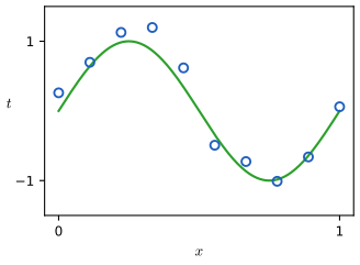
fig1_4. Download: PDF · SVG1.2.2 Linear models
p. 8 The model is the polynomial of order \(M\)
\[ y(x,\w)=w_0+w_1x+w_2x^2+\dots+w_Mx^M=\sum_{j=0}^{M}w_jx^j , \tag{1.1} \]with coefficients \(\w=(w_0,\dots,w_M)^\T\). It is nonlinear in \(x\) but linear in \(\w\): in matrix form the predictions at the training inputs are \(\Phi\w\). Models linear in their parameters are linear models (Chapter 4 of the book); everything closed-form below rests on this linearity, and it is exactly what a neural network gives up.
1.2.3 Error function
pp. 8–9 The misfit is measured by the sum-of-squares error
\[ E(\w)=\frac12\sum_{n=1}^{N}\{y(x_n,\w)-t_n\}^2 , \tag{1.2} \]half the sum of the squared vertical displacements of the points from the curve (Figure 1.5). It is non-negative and is zero exactly when the curve passes through every point. Chapter 2 of the book derives it as a negative log likelihood under Gaussian noise.
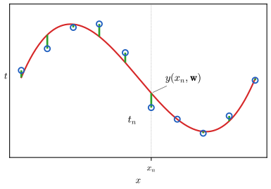
fig1_5. Download: PDF · SVGThe book states that because \(E\) is quadratic in \(\w\) its minimiser is unique and available in closed form (its Exercise 4.1). Uniqueness needs a condition that the text leaves out.
Result 1.1 (least squares: the normal equations) p. 9
\(E(\w)=\tfrac12\|\Phi\w-\tv\|^2\) is a convex quadratic with gradient \(\Phi^\T(\Phi\w-\tv)\) and Hessian \(\Phi^\T\Phi\). A minimiser always exists, and \(\w^\star\) is a minimiser if and only if it solves the normal equations
\[ \Phi^\T\Phi\,\w^\star=\Phi^\T\tv . \]The minimiser is unique if and only if \(\Phi\) has full column rank, which for the polynomial holds if and only if the inputs take at least \(M+1\) distinct values; then \(\w^\star=(\Phi^\T\Phi)^{-1}\Phi^\T\tv\). With fewer distinct inputs (for example \(M=9\) and nine points) there are infinitely many minimisers.
Proof sketch (the full proof is Result 1.1 of the companion course)
Expanding, \(E(\w+\mathbf{v})=E(\w)+\mathbf{v}^\T\Phi^\T(\Phi\w-\tv)+\tfrac12\|\Phi\mathbf{v}\|^2\). At a solution of the normal equations the middle term vanishes, so \(E(\w+\mathbf{v})\ge E(\w)\) with equality iff \(\Phi\mathbf{v}=\mathbf{0}\). A solution exists because \(\Phi^\T\tv\) lies in the column space of \(\Phi^\T\), which equals that of \(\Phi^\T\Phi\). \(\Phi\mathbf{v}=\mathbf{0}\) says the polynomial with coefficients \(\mathbf{v}\) vanishes at every \(x_n\); a non-zero polynomial of degree at most \(M\) has at most \(M\) roots, so if there are \(M+1\) distinct inputs then \(\mathbf{v}=\mathbf{0}\). Conversely, with only \(m\le M\) distinct inputs, \(\prod_{i=1}^{m}(x-\xi_i)\) (the \(\xi_i\) the distinct inputs) is a non-zero polynomial of degree \(m\le M\) vanishing at all of them, and adding any multiple of its coefficient vector to \(\w^\star\) leaves \(E\) unchanged. ∎
Filling the gap 1.2: solving the normal equations in floating point p. 9
"Closed form" does not mean "safe to compute by the formula". For the book's \(M=9\) problem the condition number of \(\Phi\) is \(1.5\times10^{7}\) and that of \(\Phi^\T\Phi\) is \(2.3\times10^{14}\), its square; forming \(\Phi^\T\Phi\) loses about 14 of the 16 significant digits of double precision.
Derivation
Let \(\Phi=\mathbf{U}\mathbf{S}\mathbf{V}^\T\) be a thin singular value decomposition (toolkit) with singular values \(s_1\ge\dots\ge s_p>0\). The 2-norm condition number is \(\kappa(\Phi)=s_1/s_p\). Since \(\Phi^\T\Phi=\mathbf{V}\mathbf{S}^2\mathbf{V}^\T\), its eigenvalues are \(s_i^2\) and \(\kappa(\Phi^\T\Phi)=s_1^2/s_p^2=\kappa(\Phi)^2\). A backward-stable solver for a linear system with matrix \(\mathbf{A}\) gives a relative error of order \(\kappa(\mathbf{A})\) times the machine precision \(u\approx1.1\times10^{-16}\); for \(\Phi^\T\Phi\) that is \(\kappa(\Phi)^2u\approx0.03\), so the computed coefficients of the order-9 fit could carry relative errors of a few per cent. A Householder QR factorisation \(\Phi=\mathbf{Q}\mathbf{R}\) works on \(\Phi\) itself: the normal equations become \(\mathbf{R}^\T\mathbf{R}\w=\mathbf{R}^\T\mathbf{Q}^\T\tv\), i.e. \(\mathbf{R}\w=\mathbf{Q}^\T\tv\) (\(\mathbf{R}\) is invertible when \(\Phi\) has full column rank), and the error is governed by \(\kappa(\Phi)\) rather than its square (for small residuals). The code and all three demos use QR. ∎
1.2.4 Model complexity
pp. 9–12 Choosing \(M\) is an instance of model selection (or model comparison). Figure 1.6 shows the least-squares fits for \(M=0,1,3,9\): the constant and the line are too rigid, the cubic is close to the sine, and the ninth-order polynomial goes through every point while oscillating wildly between them: over-fitting.
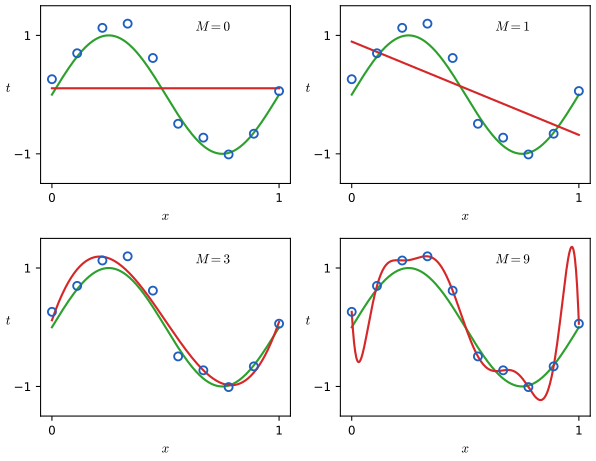
fig1_6. Download: PDF · SVGGeneralisation is measured on a test set of fresh points (100 in the book), using the root-mean-square error
\[ \Erms=\sqrt{\frac1N\sum_{n=1}^{N}\{y(x_n,\w)-t_n\}^2}=\sqrt{2E(\w)/N}, \tag{1.3} \]whose division by \(N\) puts data sets of different sizes on the same footing and whose square root returns the units of \(t\) (companion course: Definition 1.1). If a predictor \(g\) is applied to new data with noise variance \(\sigma^2\), the test \(\Erms\) estimates \(\sqrt{\E[(t-g(x))^2]}\ge\sigma\), so with our test set the best achievable value is about 0.2.
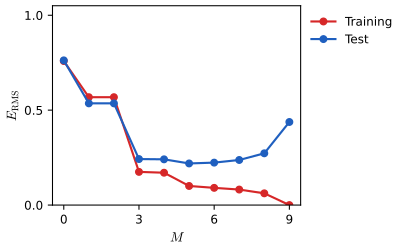
fig1_7. Download: PDF · SVG| \(M=0\) | \(M=1\) | \(M=3\) | \(M=9\) | |
|---|---|---|---|---|
| \(w_0^\star\) | 0.11 | 0.89 | 0.12 | 0.26 |
| \(w_1^\star\) | −1.58 | 11.20 | −66.13 | |
| \(w_2^\star\) | −33.66 | 1,665.69 | ||
| \(w_3^\star\) | 22.43 | −15,566.61 | ||
| \(w_4^\star\) | 76,321.23 | |||
| \(w_5^\star\) | −217,389.15 | |||
| \(w_6^\star\) | 370,626.48 | |||
| \(w_7^\star\) | −372,051.47 | |||
| \(w_8^\star\) | 202,540.70 | |||
| \(w_9^\star\) | −46,080.94 |
Table 1.1 recomputed from the recovered data. The book prints 0.90 for \(w_0^\star\) at \(M=1\) and −33.67 for \(w_2^\star\) at \(M=3\); our unrounded values are 0.8947 and −33.6607, so the differences are rounding of the targets (the \(M=9\) column fixes them only to about \(5\times10^{-3}\)). Note \(w_0^\star=\bar t=0.107\) at \(M=0\), and at \(M=1\) the line passes through \((\bar x,\bar t)\) with \(\bar x=0.5\): \(0.8947-1.5754/2=0.107\), as it must for least squares with an intercept (the residuals sum to zero).
Result 1.2 (nested models: the training error can only fall) pp. 9–11
Let \(E_M\) be the minimum of (1.2) over polynomials of order \(M\). Then \(E_0\ge E_1\ge\dots\), and if the \(N\) inputs are distinct, \(E_M=0\) for every \(M\ge N-1\): the polynomial of order \(N-1\) interpolates the data, exactly as the book observes for \(M=9\), \(N=10\).
Proof
Monotonicity. A polynomial of order \(M\) is one of order \(M+1\) with \(w_{M+1}=0\), so the set over which \(E_{M+1}\) is a minimum contains the set for \(E_M\), and a minimum over a larger set cannot be larger. This is the book's remark that "a polynomial of a given order contains all lower-order polynomials as special cases".
Interpolation. For \(M=N-1\) the design matrix is the square Vandermonde matrix, with \(\det\Phi=\prod_{1\le m\lt n\le N}(x_n-x_m)\ne0\) for distinct inputs (the determinant is a polynomial in \(x_N\) of degree \(N-1\) vanishing at \(x_1,\dots,x_{N-1}\); induction on \(N\)). So \(\Phi\w=\tv\) has a solution and \(E_{N-1}=0\); by monotonicity \(E_M=0\) for \(M\ge N-1\). ∎
This "seems paradoxical", as the book says: the order-9 family contains the cubic, the best predictor is the sine, and the sine's power series has terms of all orders. The resolution is that the failure is not a lack of flexibility but an excess of it relative to ten points.
Filling the gap 1.3: the best predictor, and why the order-9 family is not too poor p. 11
The book claims, deferring the proof, that \(\sin(2\pi x)\) is the best predictor of new data. It also invites the expectation that a richer polynomial family should do better because \(\sin(2\pi x)\) needs terms of all orders. Here are the precise statements: the best predictor under squared error is the conditional mean, and the order-9 family contains a polynomial within 0.026 of the sine everywhere on \([0,1]\), so the large test error at \(M=9\) is estimation error, not approximation error.
Derivation
The best predictor. Let \(h(x)=\E[t\given x]\) (here \(\sin(2\pi x)\)) and let \(g\) be any function of \(x\). Writing \(t-g=(t-h)+(h-g)\),
\[ \E[(t-g(x))^2]=\E[(t-h(x))^2]+2\,\E[(t-h(x))(h(x)-g(x))]+\E[(h(x)-g(x))^2]. \]Conditioning on \(x\), the middle term is \(2\,\E\big[(h(x)-g(x))\,\E[t-h(x)\given x]\big]=0\). So \(\E[(t-g)^2]=\E[\var(t\given x)]+\E[(h-g)^2]\ge\E[\var(t\given x)]\), with equality iff \(g=h\) almost everywhere. With Gaussian noise of variance \(\sigma^2\) the floor is \(\sigma^2\). (Full treatment, including other loss functions: the companion course, Section 1.5.5.)
Approximation is not the bottleneck. Expand \(f(x)=\sin(2\pi x)\) about \(x=\tfrac12\) to order 9. Taylor's theorem with the Lagrange remainder gives, for \(x\in[0,1]\), \(|f(x)-T_9(x)|=|f^{(10)}(\xi)|\,|x-\tfrac12|^{10}/10!\) for some \(\xi\). Since \(|f^{(10)}|\le(2\pi)^{10}\) and \(|x-\tfrac12|\le\tfrac12\),
\[ \max_{x\in[0,1]}|\sin(2\pi x)-T_9(x)|\le\frac{(2\pi)^{10}}{2^{10}\,10!}=\frac{\pi^{10}}{10!}\approx0.0258 . \]So some \(M=9\) polynomial is uniformly within 0.026 of the sine (the best one in least squares is within \(2\times10^{-5}\)), far below the noise level 0.2. The order-9 fit to ten points fails because its ten coefficients are determined by ten noisy numbers: the fit reproduces the noise exactly, and the nearly collinear monomials amplify it into huge coefficients (the singular-value explanation is in the companion course, Filling the gap 1.1). ∎
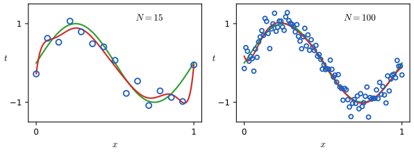
fig1_8. Download: PDF · SVGThe book quotes the classical heuristic that the number of data points should be some multiple (5 or 10) of the number of parameters, and announces that deep networks break it (Section 9.3.2 of the book). The following result quantifies what the heuristic protects against: the training error is too optimistic by an amount proportional to \(p/N\).
Result 1.3 (the optimism of the training error) pp. 10–12
Fix the inputs \(x_1,\dots,x_N\) and let \(t_n=f(x_n)+\epsilon_n\) with independent noise of mean 0 and variance \(\sigma^2\), where \(f\) is any function. Let the fitted values be \(\hat{\mathbf{y}}=\H\tv\) for a fixed matrix \(\H\) (least squares: \(\H=\Phi(\Phi^\T\Phi)^{-1}\Phi^\T\), \(\Tr\H=p\); weight decay: \(\H_\lambda=\Phi(\Phi^\T\Phi+\lambda\I)^{-1}\Phi^\T\)). Let \(\tv'\) be fresh targets at the same inputs. Then
\[ \E\Big[\tfrac1N\|\tv'-\hat{\mathbf{y}}\|^2\Big]-\E\Big[\tfrac1N\|\tv-\hat{\mathbf{y}}\|^2\Big]=\frac{2\sigma^2\,\Tr\H}{N}. \]For least squares with \(p=M+1\le N\) coefficients and \(b^2=\tfrac1N\|(\I-\H)\mathbf{f}\|^2\) (the squared bias at the inputs, \(\mathbf{f}=(f(x_n))_n\)),
\[ \E[\text{training MSE}]=b^2+\sigma^2\,\frac{N-p}{N},\qquad \E[\text{MSE on fresh targets}]=b^2+\sigma^2\,\frac{N+p}{N}. \]Proof
General \(\H\). Write \(\tv=\mathbf{f}+\bm\epsilon\), \(\tv'=\mathbf{f}+\bm\epsilon'\) with \(\bm\epsilon'\) independent of \(\bm\epsilon\). Then \(\tv'-\hat{\mathbf{y}}=(\tv-\hat{\mathbf{y}})+(\bm\epsilon'-\bm\epsilon)\) and
\[ \|\tv'-\hat{\mathbf{y}}\|^2=\|\tv-\hat{\mathbf{y}}\|^2+2(\tv-\hat{\mathbf{y}})^\T(\bm\epsilon'-\bm\epsilon)+\|\bm\epsilon'-\bm\epsilon\|^2 . \]Take expectations. \(\E\|\bm\epsilon'-\bm\epsilon\|^2=2N\sigma^2\). In the cross term, \(\tv-\hat{\mathbf{y}}=(\I-\H)(\mathbf{f}+\bm\epsilon)\) is independent of \(\bm\epsilon'\), which has mean 0, so that part vanishes, and \(\E[(\tv-\hat{\mathbf{y}})^\T\bm\epsilon]=\E[\bm\epsilon^\T(\I-\H)^\T\bm\epsilon]=\sigma^2\Tr(\I-\H)=\sigma^2(N-\Tr\H)\) (the expected quadratic form \(\E[\bm\epsilon^\T\mathbf{A}\bm\epsilon]=\sigma^2\Tr\mathbf{A}\), toolkit). Altogether the difference of expectations is \(-2\sigma^2(N-\Tr\H)+2N\sigma^2=2\sigma^2\Tr\H\); divide by \(N\).
Least squares. \(\H\) is the orthogonal projection onto the column space of \(\Phi\): symmetric, idempotent, of rank \(p\), so \(\Tr\H=p\) and \(\I-\H\) is also a projection, of rank \(N-p\). Training residuals are \((\I-\H)\mathbf{f}+(\I-\H)\bm\epsilon\); the cross term has mean 0 and \(\E\|(\I-\H)\bm\epsilon\|^2=\sigma^2\Tr(\I-\H)=\sigma^2(N-p)\), which gives the first formula, and adding \(2\sigma^2p/N\) gives the second. ∎
Reading it. At \(M=9\), \(N=10\): \(p=N\), the training error is 0 and the in-sample error is \(2\sigma^2\), twice the noise floor. With the heuristic \(N=10p\) the optimism is \(2\sigma^2/10\), a 20% overstatement of the noise floor; with \(N=5p\), 40%. For weight decay the same formula holds with \(p\) replaced by the effective number of parameters \(\Tr\H_\lambda\) (Result 1.5). Monte Carlo simulation confirms all three formulas (the optimism agrees with \(2\sigma^2p/N\) within 0.0015 for every \(M\)).
See also: Section 3.2, the bias-variance decomposition, in the companion course, which splits the expected error at a new input instead.
1.2.5 Regularization
pp. 12–13 Rather than limit the number of parameters according to the amount of data, keep the flexible model and penalise large coefficients:
\[ \widetilde{E}(\w)=\frac12\sum_{n=1}^{N}\{y(x_n,\w)-t_n\}^2+\frac{\lambda}{2}\|\w\|^2 , \tag{1.4} \]with \(\|\w\|^2=\w^\T\w=w_0^2+\dots+w_M^2\). In statistics this is a shrinkage method (ridge regression); for neural networks it is weight decay. The book notes that \(w_0\) is often left out of the penalty, because including it makes the result depend on the origin of \(t\) (Filling the gap 1.4).
See also: Section 3.1.4, regularised least squares, in the companion course.
Result 1.4 (weight decay has a unique closed-form solution) p. 13
For every \(\lambda>0\), every \(N\) and every \(M\) (even \(M+1>N\)), (1.4) is strictly convex and has the unique minimiser
\[ \w_\lambda=(\Phi^\T\Phi+\lambda\I)^{-1}\Phi^\T\tv=\sum_{i}\frac{s_i\,(\mathbf{u}_i^\T\tv)}{s_i^2+\lambda}\,\mathbf{v}_i , \]where \(\Phi=\sum_is_i\mathbf{u}_i\mathbf{v}_i^\T\) is the SVD over the non-zero singular values. Equivalently \(\w_\lambda\) is the ordinary least-squares solution of the stacked system \(\begin{pmatrix}\Phi\\ \sqrt\lambda\,\I\end{pmatrix}\w\approx\begin{pmatrix}\tv\\ \mathbf{0}\end{pmatrix}\), which is how the code computes it.
Proof sketch (full proof: companion course, Result 1.2)
The gradient is \(\Phi^\T(\Phi\w-\tv)+\lambda\w\) and the Hessian \(\Phi^\T\Phi+\lambda\I\) satisfies \(\mathbf{v}^\T(\Phi^\T\Phi+\lambda\I)\mathbf{v}=\|\Phi\mathbf{v}\|^2+\lambda\|\mathbf{v}\|^2>0\) for \(\mathbf{v}\ne\mathbf{0}\): positive definite, so the matrix is invertible and the stationary point is the unique global minimum, whatever the rank of \(\Phi\). In the SVD basis, \(\Phi^\T\Phi+\lambda\I\) acts on \(\mathbf{v}_i\) as multiplication by \(s_i^2+\lambda\) (and by \(\lambda\) on the null space of \(\Phi\), where \(\Phi^\T\tv\) has no component). The stacked system has normal equations \((\Phi^\T\Phi+\lambda\I)\w=\Phi^\T\tv\), the same. ∎
Result 1.5 (how weight decay shrinks) pp. 13–14
- \(\|\w_\lambda\|\) is non-increasing in \(\lambda\), strictly decreasing unless \(\Phi^\T\tv=\mathbf{0}\), and \(\w_\lambda\to\mathbf{0}\) as \(\lambda\to\infty\).
- As \(\lambda\to0^+\), \(\w_\lambda\to\Phi^+\tv\), the minimum-norm least-squares solution. If \(\Phi\) has full column rank this is the unique least-squares solution; if \(M+1>N\) (more coefficients than points) it is the interpolating polynomial with the smallest \(\|\w\|\).
- The effective number of parameters \(\Tr\H_\lambda=\sum_i s_i^2/(s_i^2+\lambda)\) decreases strictly from \(\rank\Phi\) (as \(\lambda\to0\)) to 0 (as \(\lambda\to\infty\)). This is the precise sense in which "\(\lambda\) controls the effective complexity of the model".
Proof
By Result 1.4, with \(c_i=\mathbf{u}_i^\T\tv\) and orthonormal \(\mathbf{v}_i\),
\[ \|\w_\lambda\|^2=\sum_i\frac{s_i^2c_i^2}{(s_i^2+\lambda)^2}. \](1) Each term is non-increasing in \(\lambda\), strictly decreasing when \(c_i\ne0\), and tends to 0 as \(\lambda\to\infty\). Since \(\Phi^\T\tv=\sum_is_ic_i\mathbf{v}_i\), some \(c_i\ne0\) unless \(\Phi^\T\tv=\mathbf{0}\).
(2) Each coefficient \(s_ic_i/(s_i^2+\lambda)\to c_i/s_i\), so \(\w_\lambda\to\sum_i(c_i/s_i)\mathbf{v}_i=\Phi^+\tv\). This vector solves the normal equations (\(\Phi^\T\Phi\Phi^+\tv=\sum_is_ic_i\mathbf{v}_i=\Phi^\T\tv\)) and lies in the row space of \(\Phi\); any other solution differs from it by a vector of the null space of \(\Phi\), which is orthogonal to the row space, so by Pythagoras every other solution has a larger norm. If \(M+1>N\) and the inputs are distinct, \(\Phi\) has rank \(N\), the least-squares solutions interpolate (\(E=0\)), and \(\Phi^+\tv\) is the smallest-norm interpolant.
(3) The fitted values are \(\H_\lambda\tv\) with \(\H_\lambda=\Phi(\Phi^\T\Phi+\lambda\I)^{-1}\Phi^\T=\sum_i\frac{s_i^2}{s_i^2+\lambda}\mathbf{u}_i\mathbf{u}_i^\T\), whose trace is the stated sum. Each term decreases strictly from 1 to 0, and there are \(\rank\Phi\) terms. ∎
On the book's data with \(M=9\): \(\Tr\H_\lambda=7.53\) at \(\ln\lambda=-18\) and \(2.15\) at \(\ln\lambda=0\). Part (2) is the bridge to the over-parameterised networks of the book's Section 9.3.2: as the penalty vanishes, the fit does not blow up but selects the smallest interpolant. For the effective number of parameters as it appears in the Bayesian evidence framework, see the companion course, Section 3.5.3.
Filling the gap 1.4: penalising \(w_0\) makes the fit depend on the origin of \(t\) p. 13
The book cites this property (via Hastie, Tibshirani and Friedman, 2009) without proof. Precisely: if \(w_0\) is not penalised, adding a constant \(c\) to every target adds exactly \(c\) to the fitted curve; if \(w_0\) is penalised, it does not.
Derivation
Let \(\mathbf{D}=\diag(0,1,\dots,1)\) and minimise \(F(\w;\tv)=\tfrac12\|\Phi\w-\tv\|^2+\tfrac\lambda2\w^\T\mathbf{D}\w\) (assume \(\Phi\) has full column rank, so the minimiser \(\w(\tv)\) is unique). The first column of \(\Phi\) is \(\mathbf{1}\), so with \(\mathbf{e}_0=(1,0,\dots,0)^\T\) we have \(\Phi(\w+c\,\mathbf{e}_0)=\Phi\w+c\mathbf{1}\) and \(\mathbf{D}\mathbf{e}_0=\mathbf{0}\). Hence
\[ F(\w+c\,\mathbf{e}_0;\ \tv+c\mathbf{1})=F(\w;\tv)\quad\text{for every }\w , \]so the minimiser for the shifted targets is \(\w(\tv)+c\,\mathbf{e}_0\), and the fitted curve moves up by exactly \(c\). If \(w_0\) is penalised (\(\mathbf{D}=\I\)) this fails already for \(M=0\): \(\widetilde E=\tfrac12\sum_n(w_0-t_n)^2+\tfrac\lambda2w_0^2\) is minimised by \(w_0=\sum_nt_n/(N+\lambda)\), and shifting every target by \(c\) moves the fit by \(Nc/(N+\lambda)\ne c\). The fitted curve then depends on where the zero of \(t\) is placed, which a model of \(t\) should not. ∎
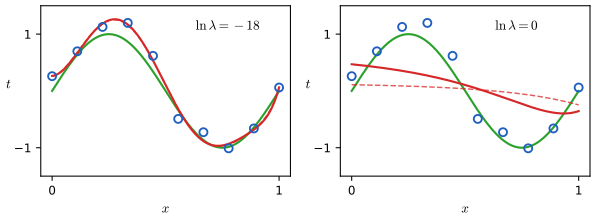
fig1_9. Download: PDF · SVG| \(\ln\lambda=-\infty\) | \(\ln\lambda=-18\), (1.4) | \(\ln\lambda=0\), (1.4) | \(\ln\lambda=-18\), \(N\lambda\) | \(\ln\lambda=0\), \(N\lambda\) | |
|---|---|---|---|---|---|
| \(w_0^\star\) | 0.26 | 0.26 | 0.47 | 0.26 | 0.11 |
| \(w_1^\star\) | −66.13 | 0.24 | −0.40 | 0.64 | −0.07 |
| \(w_2^\star\) | 1,665.69 | 45.50 | −0.46 | 43.69 | −0.09 |
| \(w_3^\star\) | −15,566.61 | −137.63 | −0.32 | −144.00 | −0.07 |
| \(w_4^\star\) | 76,321.23 | 12.55 | −0.17 | 57.90 | −0.05 |
| \(w_5^\star\) | −217,389.15 | 190.70 | −0.05 | 117.36 | −0.04 |
| \(w_6^\star\) | 370,626.48 | −5.04 | 0.05 | 9.87 | −0.02 |
| \(w_7^\star\) | −372,051.47 | −145.84 | 0.12 | −90.02 | −0.01 |
| \(w_8^\star\) | 202,540.70 | −30.07 | 0.18 | −70.90 | −0.01 |
| \(w_9^\star\) | −46,080.94 | 69.38 | 0.22 | 75.26 | 0.00 |
Erratum: the \(\lambda\) of Table 1.2 (and Figures 1.9, 1.10) is \(N\) times the \(\lambda\) of (1.4) pp. 13–14
With the book's own training data (recovered above), the two regularised columns of Table 1.2 are reproduced to every printed digit (largest difference 0.007, rounding) by minimising (1.4) with \(\lambda\) replaced by \(N\lambda=10\lambda\), equivalently by minimising the mean squared error \(\frac1{2N}\sum_n\{y(x_n,\w)-t_n\}^2+\frac\lambda2\|\w\|^2\). With (1.4) exactly as printed, the coefficients are those of the second and third columns above, which differ from the printed ones by up to 73. In other words, the printed labels \(\ln\lambda=-18\) and \(0\) correspond to \(\ln\lambda=-18+\ln10\approx-15.70\) and \(\ln\lambda=2.30\) in (1.4). The book's Figure 1.9 (right panel nearly flat) matches the \(N\lambda\) convention too. The difference is a shift of the \(\ln\lambda\) axis by \(\ln N\) and changes none of the conclusions. The table above shows both; the curve-fitting demo has a switch between them.
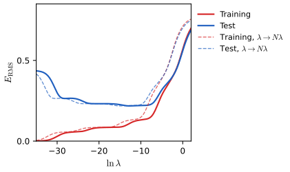
fig1_10. Download: PDF · SVG1.2.6 Model selection
pp. 14–15 \(\lambda\) and \(M\) are hyperparameters: fixed while \(\w\) is fitted. They cannot be fitted on the training error, because that always prefers \(\lambda\to0\) and large \(M\) (Results 1.2 and 1.6).
Result 1.6 (minimising jointly over \(\w\) and \(\lambda\) drives \(\lambda\) to 0) p. 14
Let \(V(\lambda)=\min_\w\widetilde E(\w,\lambda)\) for \(\lambda\ge0\). Then \(V\) is non-decreasing and continuous, with derivative \(V'(\lambda)=\tfrac12\|\w_\lambda\|^2\) for \(\lambda>0\); it is strictly increasing unless \(\Phi^\T\tv=\mathbf{0}\). So the infimum of \(\widetilde E\) over \((\w,\lambda)\) is attained at \(\lambda=0\), at the unregularised (over-fitted) least-squares solution.
Proof
For \(\lambda_1\lt\lambda_2\) and every \(\w\), \(\widetilde E(\w,\lambda_1)\le\widetilde E(\w,\lambda_2)\); minimising both sides over \(\w\) gives \(V(\lambda_1)\le V(\lambda_2)\). For \(\lambda>0\), \(V(\lambda)=\widetilde E(\w_\lambda,\lambda)\) with \(\w_\lambda\) differentiable in \(\lambda\) (Result 1.4, a smooth matrix inverse). By the chain rule \(V'(\lambda)=\nabla_\w\widetilde E(\w_\lambda,\lambda)^\T\,\frac{\d\w_\lambda}{\d\lambda}+\frac{\partial\widetilde E}{\partial\lambda}(\w_\lambda,\lambda)\), and the first term vanishes because \(\w_\lambda\) is a stationary point (the envelope theorem), leaving \(\tfrac12\|\w_\lambda\|^2\), which is positive unless \(\w_\lambda=\mathbf{0}\), i.e. unless \(\Phi^\T\tv=\mathbf{0}\). Continuity at 0: \(V(0)\le V(\lambda)\le\widetilde E(\w^+,\lambda)=V(0)+\tfrac\lambda2\|\w^+\|^2\) with \(\w^+=\Phi^+\tv\). The same argument with nested model sets (Result 1.2) shows that the training error, minimised over \(M\) as well, picks the largest \(M\). ∎
The remedy is to hold data out. Split the data into a training set (to fit \(\w\)) and a validation (hold-out, development) set (to compare hyperparameter values); if the design is iterated many times, the validation set is itself over-fitted, and a third test set is kept for the final assessment. For a fixed fitted function \(g\), the validation mean squared error is an average of \(N_{\rm v}\) independent terms \((t_n-g(x_n))^2\), so it is an unbiased estimate of \(g\)'s expected squared error with variance \(\var[(t-g(x))^2]/N_{\rm v}\): small validation sets give noisy estimates, which is the dilemma that cross-validation addresses.
See also: Section 1.3, model selection (cross-validation, AIC, BIC), in the companion course.
S-fold cross-validation trains on a fraction \((S-1)/S\) of the data in each run while every point is used for validation exactly once; \(S=N\) is leave-one-out. Its costs, as the book notes: \(S\) training runs per hyperparameter setting, and a grid of \(K\) values for each of \(h\) hyperparameters needs \(S\,K^h\) runs, exponential in \(h\). For models that are linear in their parameters, leave-one-out costs no more than a single fit:
Result 1.7 (leave-one-out without refitting) p. 15
For least squares or weight decay (\(\lambda\ge0\), with \(\Phi^\T\Phi+\lambda\I\) invertible), let \(\H=\Phi(\Phi^\T\Phi+\lambda\I)^{-1}\Phi^\T\) and \(\hat y_n=(\H\tv)_n\). If \(\hat y^{(-n)}\) is the prediction at \(x_n\) of the model refitted without point \(n\), then
\[ t_n-\hat y^{(-n)}=\frac{t_n-\hat y_n}{1-H_{nn}}\qquad(H_{nn}\lt1). \]So the leave-one-out error is \(\frac1N\sum_n\big((t_n-\hat y_n)/(1-H_{nn})\big)^2\), from one fit. If \(H_{nn}=1\) the point cannot be predicted from the others: this happens for every point at \(M=9\), \(N=10\), \(\lambda=0\), where each nine-point fit is not unique (Result 1.1).
Proof
Let \(\mathbf{A}=\Phi^\T\Phi+\lambda\I\), \(\bm\phi_n\) the \(n\)th row of \(\Phi\) as a column vector, so \(H_{nn}=\bm\phi_n^\T\mathbf{A}^{-1}\bm\phi_n\). Removing point \(n\) gives \(\mathbf{A}_{-n}=\mathbf{A}-\bm\phi_n\bm\phi_n^\T\) and right-hand side \(\Phi^\T\tv-\bm\phi_nt_n\). By the Sherman–Morrison formula (valid since \(1-H_{nn}\ne0\)),
\[ \mathbf{A}_{-n}^{-1}=\mathbf{A}^{-1}+\frac{\mathbf{A}^{-1}\bm\phi_n\bm\phi_n^\T\mathbf{A}^{-1}}{1-H_{nn}} . \]Hence, with \(\w=\mathbf{A}^{-1}\Phi^\T\tv\) and \(\hat y_n=\bm\phi_n^\T\w\),
\[ \hat y^{(-n)}=\bm\phi_n^\T\mathbf{A}_{-n}^{-1}(\Phi^\T\tv-\bm\phi_nt_n)=\hat y_n-H_{nn}t_n+\frac{H_{nn}(\hat y_n-H_{nn}t_n)}{1-H_{nn}}=\frac{\hat y_n-H_{nn}t_n}{1-H_{nn}} . \]Then \(t_n-\hat y^{(-n)}=\frac{t_n-H_{nn}t_n-\hat y_n+H_{nn}t_n}{1-H_{nn}}=\frac{t_n-\hat y_n}{1-H_{nn}}\). If \(H_{nn}=1\) (and \(\lambda=0\)), \(\mathbf{A}_{-n}=\Phi_{-n}^\T\Phi_{-n}\) is singular because \(\bm\phi_n^\T\mathbf{A}^{-1}\) is a null vector of it, so the reduced fit is not unique. ∎
A comparison of the formula with \(N\) explicit refits gives agreement to \(2\times10^{-11}\) or better. On the book's data the leave-one-out \(\Erms\) for \(M=0,\dots,8\) is 0.843, 0.729, 1.004, 0.351, 0.686, 0.419, 0.955, 4.01, 19.4: with ten points the estimate is itself very noisy, and the cubic wins.
A further observation from the demo: with only 7 or 8 training points per run, the ninth-order polynomial is under-determined, and as \(\lambda\to0\) each run's fit tends to its minimum-norm interpolant (Result 1.5(2)), which predicts the held-out points badly; this is why the cross-validation curve rises steeply on the left even though the full-data training error falls. Modern practice, as the book stresses, can afford little such exploration for very large models and relies on experience with smaller models and on heuristics.
The section ends by listing what changes for real applications: far more data, many inputs and outputs, models with up to hundreds of billions of parameters, a highly nonlinear error function with no closed-form minimiser, and therefore iterative optimisation based on derivatives (Chapters 7 and 8 of the book).
1.3 A brief history of machine learning
pp. 16–17 Neural networks began as models of the brain: about 90 billion neurons, each with several thousand synapses, some \(10^{14}\) connections in all, whose strengths change as we learn (Figure 1.12, a drawing, is not reproduced). The simplest mathematical model of a neuron (McCulloch and Pitts, 1943) forms a weighted sum of its inputs and passes it through a nonlinearity:
\[ a=\sum_{i=1}^{M}w_ix_i , \tag{1.5} \] \[ y=f(a) , \tag{1.6} \]with weights \(w_i\), pre-activation \(a\), activation function \(f\) and activation \(y\) (Figure 1.13).
Filling the gap 1.6: the polynomial (1.1) as a neuron needs a constant input p. 17
The book says the polynomial (1.1) is "a specific instance" of (1.5)–(1.6) with inputs \(x_i=x^i\) and \(f(a)=a\). As printed, (1.5) sums from \(i=1\) and so has no constant term, while (1.1) has \(w_0\).
Derivation
Add an input \(x_0\equiv1\) (or, equivalently, a bias \(w_0\) added to \(a\)): \(a=\sum_{i=0}^{M}w_ix_i\). With \(x_i=x^i\) for \(i=0,\dots,M\) (so \(x_0=x^0=1\)) and \(f(a)=a\), \(y=\sum_{i=0}^{M}w_ix^i=y(x,\w)\), which is (1.1). Without the constant input, (1.5) with \(x_i=x^i\), \(i\ge1\), gives only polynomials with \(y(0)=0\), and the sine-plus-noise data (with \(t_1=0.26\) at \(x=0\)) could not be fitted exactly at \(M=9\). The same device (a unit with constant output 1) carries the biases of every layer in later chapters. ∎
1.3.1 Single-layer networks
pp. 17–18 The first phase is networks with one layer of adjustable weights. The most important is Rosenblatt's perceptron, whose activation is the step function
\[ f(a)=\begin{cases}0, & a\le0,\\ 1, & a>0,\end{cases} \tag{1.7} \]a crude model of a neuron that fires when its total input exceeds a threshold. Its learning rule has the property, stated in the book with a reference to Bishop (2006), that if some weight vector classifies the training data perfectly then the algorithm finds one in a finite number of steps. The book uses targets \(t\in\{0,1\}\) matched to (1.7); the theorem and proof read as follows in that convention.
See also: Section 4.1.7, the perceptron algorithm, in the companion course (with targets \(\pm1\) and fixed features).
Algorithm 1.1 (the perceptron with 0/1 targets) p. 17, (1.7)
Augment each input with \(x_0=1\), so \(\tilde\x_n=(1,\x_n)\). Start from \(\w=\mathbf{0}\). Visit the patterns cyclically; at pattern \(n\) compute \(f(\w^\T\tilde\x_n)\) and set
\[ \w\leftarrow\w+\big(t_n-f(\w^\T\tilde\x_n)\big)\,\tilde\x_n . \]Stop after a full pass with no change. The update is zero on a correctly classified pattern; on a mistake it adds \(\tilde\x_n\) (if \(t_n=1\)) or subtracts it (if \(t_n=0\)). With \(s_n=2t_n-1\in\{-1,+1\}\), a mistake means \(s_n\w^\T\tilde\x_n\le0\) and the update is \(\w\leftarrow\w+s_n\tilde\x_n\), the familiar \(\pm1\) form.
Result 1.8 (perceptron convergence theorem; Novikoff, 1962) p. 17
Suppose the data are linearly separable with margin \(\gamma>0\): there is a unit vector \(\w^\ast\) with \(s_n\,\w^{\ast\T}\tilde\x_n\ge\gamma\) for all \(n\). Let \(R=\max_n\|\tilde\x_n\|\). Then Algorithm 1.1 makes at most \((R/\gamma)^2\) updates, after which it classifies every training point correctly and stops.
Proof (the same argument with \(\pm1\) targets is in the companion course, Result 4.7)
Let \(\w_k\) be the weight vector after \(k\) updates, \(\w_0=\mathbf{0}\), and suppose update \(k+1\) is made on pattern \(n\), so \(\w_{k+1}=\w_k+s_n\tilde\x_n\) with \(s_n\w_k^\T\tilde\x_n\le0\) (a mistake: for \(t_n=1\), \(f=0\) means \(\w_k^\T\tilde\x_n\le0\); for \(t_n=0\), \(f=1\) means \(\w_k^\T\tilde\x_n>0\)).
Progress along \(\w^\ast\). \(\w^{\ast\T}\w_{k+1}=\w^{\ast\T}\w_k+s_n\w^{\ast\T}\tilde\x_n\ge\w^{\ast\T}\w_k+\gamma\), so by induction \(\w^{\ast\T}\w_k\ge k\gamma\).
Slow growth of the norm. \(\|\w_{k+1}\|^2=\|\w_k\|^2+2s_n\w_k^\T\tilde\x_n+\|\tilde\x_n\|^2\le\|\w_k\|^2+R^2\), because the middle term is \(\le0\) at a mistake; so \(\|\w_k\|^2\le kR^2\).
Combine. By Cauchy–Schwarz, \(k\gamma\le\w^{\ast\T}\w_k\le\|\w_k\|\le\sqrt k\,R\), i.e. the cosine of the angle between \(\w_k\) and \(\w^\ast\) is at least \(\sqrt k\,\gamma/R\), and a cosine cannot exceed 1. Hence \(k\le(R/\gamma)^2\). Since the algorithm only stops after a pass without mistakes, and there can be at most \((R/\gamma)^2\) mistakes in total, it stops after at most \((R/\gamma)^2+1\) passes with all points correctly classified. ∎
Remarks. (i) The best bound uses the largest margin \(\gamma^\ast=\max_{\|\w\|=1}\min_ns_n\w^\T\tilde\x_n\), which is the distance from the origin to the convex hull of the points \(s_n\tilde\x_n\) (the code computes it this way). (ii) The bound says nothing for non-separable data, where the algorithm never stops. (iii) A numerical run verifies \(\w^{\ast\T}\w_k\ge k\gamma\) and \(\|\w_k\|^2\le kR^2\) after every update of a run: on the demo's data with margin 0.15 the run stops after 4 updates, against \((R/\gamma^\ast)^2=60\) with the largest margin (the demo shows the weaker bound 98 from the margin of the generating line).
The book reports that Minsky and Papert (1969) proved formal limits of single-layer networks. The classic example is exclusive or:
Result 1.9 (XOR is not linearly separable; two layers suffice)
No weights \((w_0,w_1,w_2)\) make \(f(w_0+w_1x_1+w_2x_2)\) equal \(x_1\oplus x_2\) on \(\{0,1\}^2\) (targets \(0,1,1,0\) at \((0,0),(0,1),(1,0),(1,1)\)). But two layers of step units do it:
\[ h_1=f(x_1+x_2-\tfrac12),\qquad h_2=f(x_1+x_2-\tfrac32),\qquad y=f(h_1-h_2-\tfrac12). \]Proof
Impossibility. Correct classification requires \(a(0,0)=w_0\le0\), \(a(1,1)=w_0+w_1+w_2\le0\), \(a(0,1)=w_0+w_2>0\) and \(a(1,0)=w_0+w_1>0\). Adding the last two gives \(2w_0+w_1+w_2>0\); adding the first two gives \(2w_0+w_1+w_2\le0\). Contradiction. (Geometrically: the midpoint \((\tfrac12,\tfrac12)\) of the two class-1 points equals the midpoint of the two class-0 points, and the pre-activation, being affine, takes the same value there from both pairs.)
Two layers. \(h_1\) is the OR of the inputs (sum at least 1) and \(h_2\) the AND (sum equal to 2). Then \(h_1-h_2\) is 1 exactly when one input is 1, so \(y=f(h_1-h_2-\tfrac12)\) is XOR: inputs \((0,0)\to(h_1,h_2)=(0,0)\to y=0\); \((0,1),(1,0)\to(1,0)\to y=1\); \((1,1)\to(1,1)\to y=0\). ∎
Running Algorithm 1.1 on XOR, the weight vector returns to a previous value within a few passes and cycles for ever (confirmed numerically). The construction shows that the limitation is in learning, not representation: the perceptron rule trains only one layer, and nothing like it was known for the hidden layer.
The book's Figure 1.14 (photographs of the Mark 1 perceptron hardware) is not reproduced. A typical perceptron had several layers of processing but only one learnable layer; the name survives in the multilayer perceptron (MLP).
1.3.2 Backpropagation
pp. 18–20 Two changes made multilayer training possible: differentiable activation functions with non-zero gradient in place of (1.7), and differentiable error functions such as (1.2). The first change is essential, for the following reason.
Filling the gap 1.7: a network of step units has zero gradient almost everywhere p. 18
The book says the step function had to be replaced by an activation "having a non-zero gradient". Precisely: for a network of step units and any error that depends on the weights only through the outputs, the error is piecewise constant in the weights, so its gradient is zero wherever it exists, and gradient descent never moves.
Derivation
Fix the finite training set. Each unit's output is \(f(a)\) with \(a\) an affine function of the weights and of the outputs of earlier units. Proceed layer by layer: suppose the outputs of all earlier units are locally constant at a weight vector \(\w\). Then the pre-activation of the current unit on pattern \(n\) is affine in its own weights, and if it is non-zero it keeps its sign in a neighbourhood of \(\w\), so the unit's output is locally constant too. The weight vectors at which some pre-activation equals exactly zero for some pattern lie in a finite union of hyperplanes (for each of the finitely many possible configurations of earlier outputs, the pre-activation is a non-constant affine function of the unit's own weights, because the bias input is 1), a set of Lebesgue measure zero. Off that set every output, hence the error, is locally constant: all partial derivatives are zero. On the set, the error jumps and has no derivative. Either way the gradient carries no information about which way to move. Numerically, every finite-difference derivative of the error of a random step network on XOR is exactly 0. ∎
Nodes in the middle layer are hidden units: their values are not in the training data. Training initialises the weights at random and repeatedly moves them against the gradient of the error; the gradient is computed efficiently by error backpropagation (Rumelhart, Hinton and Williams, 1986), and the most common optimiser is stochastic gradient descent (Chapters 7 and 8 of the book). For the network used in the demo the whole calculation fits in a few lines.
Result 1.10 (backpropagation for a two-layer network)
Take inputs \(\x\in\R^D\), \(H\) hidden units \(z_j=\tanh(a_j)\) with \(a_j=w^{(1)}_{j0}+\sum_iw^{(1)}_{ji}x_i\), one output \(y=\sigma(a)\) with \(a=w^{(2)}_0+\sum_jw^{(2)}_jz_j\) and \(\sigma\) the logistic sigmoid, and the cross-entropy \(E_n=-t\ln y-(1-t)\ln(1-y)\). Then, with \(x_0=z_0=1\),
\[ \delta\equiv\frac{\partial E_n}{\partial a}=y-t,\qquad \frac{\partial E_n}{\partial w^{(2)}_j}=\delta\,z_j,\qquad \delta_j\equiv\frac{\partial E_n}{\partial a_j}=(1-z_j^2)\,w^{(2)}_j\,\delta,\qquad \frac{\partial E_n}{\partial w^{(1)}_{ji}}=\delta_j\,x_i . \]One forward pass and one backward pass give all \((D+1)H+H+1\) derivatives in a number of operations proportional to the number of weights.
Proof
Since \(\sigma'(a)=\sigma(a)(1-\sigma(a))\), \(\partial E_n/\partial a=\big(-t/y+(1-t)/(1-y)\big)y(1-y)=-t(1-y)+(1-t)y=y-t\). The output pre-activation depends on \(w^{(2)}_j\) only through the term \(w^{(2)}_jz_j\), so \(\partial a/\partial w^{(2)}_j=z_j\). The hidden pre-activation \(a_j\) affects \(E_n\) only through \(z_j\) and then \(a\): by the chain rule \(\partial E_n/\partial a_j=\delta\cdot w^{(2)}_j\cdot\tanh'(a_j)\) with \(\tanh'=1-\tanh^2\). Finally \(\partial a_j/\partial w^{(1)}_{ji}=x_i\). Each derivative is a product of quantities already computed in the forward pass and one \(\delta\), hence the linear cost. The general recursion for any feed-forward network is Chapter 8 of the book; the companion course derives it in Section 5.3. These formulas agree with central differences and with PyTorch's automatic differentiation (to \(10^{-12}\)). ∎
A plateau. In the demo, a network with two hidden units started from one particular seed stalls at mean cross-entropy \(\ln2/2\approx0.3466\). That number has a simple origin: two of the four XOR patterns are fitted (loss near 0) and the other two sit at \(y=\tfrac12\) (loss \(\ln2\) each), so the mean is \(2\ln2/4\). Training from other initial weights, or with three hidden units, escapes it.
See also: Section 5.1, feed-forward network functions (and universal approximation, Result 5.1), and the backpropagation demo, in the companion course.
The 1980s revival also brought a more principled view, rooted in probability and statistics (Bishop, 1995): learning needs background assumptions, inductive biases, built in explicitly (for example making a lesion classifier insensitive to where the lesion is in the image) or implicitly through the form of the model and its training. Yet only the last two layers of deeper networks seemed to learn useful weights; apart from convolutional networks (LeCun et al., 1998), practical systems relied on hand-crafted feature extraction, and by 2000 kernel methods, support vector machines and Gaussian processes had largely displaced neural networks.
1.3.3 Deep networks
pp. 20–22 The third phase, from about 2010, trains networks with many layers: deep neural networks and deep learning (LeCun, Bengio and Hinton, 2015). Its ingredients were scale (from thousands of parameters in the 1980s to about \(10^{12}\) now, with commensurate data and compute on GPUs; Krizhevsky, Sutskever and Hinton, 2012), and technical advances such as residual connections and automatic differentiation.
Filling the gap 1.8: the arithmetic of Figure 1.16 p. 21
The book's Figure 1.16, a chart of training compute against date reprinted from OpenAI, is not reproduced (its data are not in the book). The numbers in its discussion check out:
Derivation
A petaflop/s-day is \(10^{15}\ \text{operations/s}\times86{,}400\ \text{s}=8.64\times10^{19}\) operations, "roughly \(10^{20}\)". The top of the chart, about \(10^4\) petaflop/s-days, is \(8.6\times10^{23}\approx10^{24}\) operations. A doubling time of \(T\) months multiplies compute by \(2^{12/T}\) per year: \(2^{12/24}=\sqrt2\approx1.41\) for the two-year doubling before 2012 (Moore's law), and \(2^{12/3.4}\approx11.5\) for the 3.4-month doubling after, the book's "factor of 10 increase every year". Over the decade 2012–2022 the second rate compounds to about \(11.5^{10}\approx4\times10^{10}\). ∎
A trained deep network can be seen as performing representation learning (Bengio, Courville and Vincent, 2012): its hidden layers map the input to a representation in which the final layers have an easy problem, and such representations can be reused through transfer learning; large networks adapted to many downstream tasks are foundation models (Bommasani et al., 2021). Gains from clever architecture are often overtaken by simply scaling data, model and compute (Sutton, 2019). The chapter's remark that "the training signals become weaker as they are backpropagated through successive layers", and that residual connections (He et al., 2015) cure this, has a precise form:
Result 1.11 (the backpropagated signal through a deep chain) p. 22
Consider a chain of \(L\) layers \(\mathbf{z}^{(l)}=\bm\sigma(\mathbf{W}_l\mathbf{z}^{(l-1)})\) (logistic sigmoid applied elementwise), and an error \(E\) of the output \(\mathbf{z}^{(L)}\). With \(\mathbf{g}^{(l)}=\partial E/\partial\mathbf{z}^{(l)}\) and \(\mathbf{D}_l=\diag\big(\sigma'(\mathbf{W}_l\mathbf{z}^{(l-1)})\big)\),
\[ \mathbf{g}^{(l-1)}=\mathbf{W}_l^\T\mathbf{D}_l\,\mathbf{g}^{(l)}, \] \[ \|\mathbf{g}^{(0)}\|\le\Big(\tfrac14\Big)^L\prod_{l=1}^{L}\|\mathbf{W}_l\|\;\|\mathbf{g}^{(L)}\| \](\(\|\cdot\|\) the spectral norm for matrices). For a residual chain \(\mathbf{z}^{(l)}=\mathbf{z}^{(l-1)}+\bm\sigma(\mathbf{W}_l\mathbf{z}^{(l-1)})-\tfrac12\mathbf{1}\) the recursion becomes \(\mathbf{g}^{(l-1)}=(\I+\mathbf{W}_l^\T\mathbf{D}_l)\mathbf{g}^{(l)}\), and if \(\varepsilon_l=\|\mathbf{D}_l\mathbf{W}_l\|\lt1\),
\[ \|\mathbf{g}^{(0)}\|\ge\prod_{l=1}^{L}(1-\varepsilon_l)\;\|\mathbf{g}^{(L)}\|, \]which is at least \(e^{-2\sum_l\varepsilon_l}\|\mathbf{g}^{(L)}\|\) when every \(\varepsilon_l\le\tfrac12\).
Proof
Recursion. \(z^{(l)}_i=\sigma(a_i)\) with \(a_i=\sum_jW_{l,ij}z^{(l-1)}_j\), so \(\partial z^{(l)}_i/\partial z^{(l-1)}_j=\sigma'(a_i)W_{l,ij}\); the Jacobian is \(\mathbf{D}_l\mathbf{W}_l\) and the chain rule gives \(\mathbf{g}^{(l-1)}=(\mathbf{D}_l\mathbf{W}_l)^\T\mathbf{g}^{(l)}\). In the residual chain the Jacobian is \(\I+\mathbf{D}_l\mathbf{W}_l\).
Upper bound. \(\sigma'(a)=\sigma(a)(1-\sigma(a))\le\tfrac14\) (the product of two numbers summing to 1 is at most \(\tfrac14\)), so \(\|\mathbf{D}_l\|\le\tfrac14\), and submultiplicativity of the spectral norm (with \(\|\mathbf{A}^\T\|=\|\mathbf{A}\|\)) gives \(\|\mathbf{g}^{(l-1)}\|\le\tfrac14\|\mathbf{W}_l\|\,\|\mathbf{g}^{(l)}\|\); iterate. Unless the weights grow (which saturates the units and makes \(\sigma'\) even smaller), the signal reaching the first layers decays geometrically.
Lower bound. For any matrix \(\mathbf{A}\) with \(\|\mathbf{A}\|\lt1\) and vector \(\mathbf{v}\), \(\|(\I+\mathbf{A}^\T)\mathbf{v}\|\ge\|\mathbf{v}\|-\|\mathbf{A}^\T\mathbf{v}\|\ge(1-\|\mathbf{A}\|)\|\mathbf{v}\|\) (reverse triangle inequality). Apply with \(\mathbf{A}=\mathbf{D}_l\mathbf{W}_l\) and iterate. Finally \(1-\varepsilon\ge e^{-2\varepsilon}\) for \(0\le\varepsilon\le\tfrac12\) (the function \(e^{-2\varepsilon}\) is convex, equals \(1-\varepsilon\) at 0, and \(e^{-1}\lt\tfrac12\) at \(\varepsilon=\tfrac12\), so the chord lies above it). ∎
Numbers. For \(L=30\), width 16 and weights \(\N(0,1/16)\) (the demo's default), the signal at the input is \(2.4\times10^{-20}\) of its value at the output in the plain chain and 1.76 times it in the residual chain; both agree with PyTorch's automatic differentiation, and both bounds hold numerically. The identity path in \(\I+\mathbf{D}_l\mathbf{W}_l\) is what lets networks with hundreds of layers train (Section 9.5 of the book).
The last development the book highlights is automatic differentiation: the backward pass is generated from the code of the forward pass, so only forward functions need to be written; it (PyTorch) confirms the hand-written backpropagation of Results 1.10 and 1.11 numerically. Open-source software and shared research have accelerated the field further.
Exercises
Chapter 1 of the book has no end-of-chapter exercises (they start with Chapter 2). The text refers to Exercises 4.1 and 4.2 for the closed-form solutions of (1.2) and (1.4); those are derived above in Result 1.1 and Result 1.4, and will be solved in full with Chapter 4.
Demonstrations for this chapter
Each demonstration runs in the browser with seeded random numbers (the same generator as the Python code, so the pages reproduce the numbers of the Python code), and links back to these notes. The ▶ Demo boxes above open them already set to the case under discussion.
| Demonstration | What you can see | Sections and results |
|---|---|---|
| Polynomial curve fitting: order, data size and weight decay | The book's own ten points, least-squares and regularised polynomials of order 0 to 9, the coefficients (Tables 1.1 and 1.2), training and test error against \(M\) and against \(\ln\lambda\), the effective number of parameters, and the two \(\lambda\) conventions. Presets: 1 orders 0, 1, 3, 9 (Fig. 1.6); 2 M = 9 interpolates (Table 1.1, Fig. 1.7); 3 more data (Fig. 1.8); 4 weight decay (Figs. 1.9, 1.10); 5 the \(\lambda\) convention of Table 1.2. | 1.2.1–1.2.5; Results 1.1, 1.2, 1.4, 1.5 |
| Model selection: cross-validation and the optimism of the training error | The folds of S-fold cross-validation (Fig. 1.11), the fits of each run, cross-validation, training and test error against \(\ln\lambda\) or \(M\), reshuffled partitions, the cost count, and a Monte Carlo of the training error against fresh-target error with the exact formulas. Presets: 1 4-fold over \(\ln\lambda\); 2 leave-one-out; 3 reshuffled folds; 4 choosing \(M\); 5 optimism \(2\sigma^2p/N\). | 1.2.4, 1.2.6; Results 1.3, 1.6, 1.7 |
| Three phases of neural networks: perceptron, backpropagation, depth | The perceptron on separable data with the cosine bound of the convergence proof, its cycling on XOR, a 2-H-1 network trained by backpropagation on XOR with its hidden-unit lines and loss curve, and the backpropagated signal against depth with and without residual connections. Presets: 1 perceptron; 2 XOR fails; 3 two layers solve XOR; 4 a plateau; 5 depth and residual connections. | 1.3.1–1.3.3; Results 1.8–1.11 |
The Python code that produces every figure of this page is code/ch01_deep_learning_revolution.py (see the code index). Figures 1.1, 1.2, 1.3, 1.12, 1.14 and 1.16 are photographs, drawings or charts reprinted from other sources and are not reproduced.
References
- Bishop, C. M. and Bishop, H. (2024). Deep Learning: Foundations and Concepts. Springer, Cham. Chapter 1, pp. 1–22. doi:10.1007/978-3-031-45468-4.
- Bishop, C. M. (1995). Neural Networks for Pattern Recognition. Oxford University Press.
- Bishop, C. M. (2006). Pattern Recognition and Machine Learning. Springer, New York.
- Bengio, Y., Courville, A. and Vincent, P. (2012). Representation learning: a review and new perspectives. arXiv:1206.5538.
- Bommasani, R. et al. (2021). On the opportunities and risks of foundation models. arXiv:2108.07258.
- Esteva, A., Kuprel, B., Novoa, R. A., Ko, J., Swetter, S. M., Blau, H. M. and Thrun, S. (2017). Dermatologist-level classification of skin cancer with deep neural networks. Nature, 542, 115–118. doi:10.1038/nature21056.
- Hastie, T., Tibshirani, R. and Friedman, J. (2009). The Elements of Statistical Learning, 2nd edition. Springer, New York.
- He, K., Zhang, X., Ren, S. and Sun, J. (2015). Deep residual learning for image recognition. arXiv:1512.03385.
- Jumper, J. et al. (2021). Highly accurate protein structure prediction with AlphaFold. Nature, 596, 583–589. doi:10.1038/s41586-021-03819-2.
- Krizhevsky, A., Sutskever, I. and Hinton, G. E. (2012). ImageNet classification with deep convolutional neural networks. In Advances in Neural Information Processing Systems 25, 1097–1105.
- LeCun, Y., Bengio, Y. and Hinton, G. (2015). Deep learning. Nature, 521, 436–444. doi:10.1038/nature14539.
- LeCun, Y., Bottou, L., Bengio, Y. and Haffner, P. (1998). Gradient-based learning applied to document recognition. Proceedings of the IEEE, 86(11), 2278–2324. doi:10.1109/5.726791.
- McCulloch, W. S. and Pitts, W. (1943). A logical calculus of the ideas immanent in nervous activity. Bulletin of Mathematical Biophysics, 5, 115–133. doi:10.1007/BF02478259.
- Minsky, M. L. and Papert, S. A. (1969). Perceptrons. MIT Press, Cambridge, MA.
- Novikoff, A. B. J. (1962). On convergence proofs on perceptrons. In Proceedings of the Symposium on the Mathematical Theory of Automata, Vol. 12, 615–622. Polytechnic Institute of Brooklyn.
- Rosenblatt, F. (1962). Principles of Neurodynamics: Perceptrons and the Theory of Brain Mechanisms. Spartan, Washington, DC.
- Rumelhart, D. E., Hinton, G. E. and Williams, R. J. (1986). Learning representations by back-propagating errors. Nature, 323, 533–536. doi:10.1038/323533a0.
- Sutton, R. (2019). The bitter lesson. Essay, 13 March 2019.
The numerical statements in the text (the recovered training set and Tables 1.1 and 1.2, the optimism formulas, the shrinkage and minimum-norm limits, the leave-one-out formula, the perceptron bound along a run, XOR, the zero gradient of step networks, backpropagation against finite differences and automatic differentiation, the depth bounds and the compute arithmetic) were confirmed numerically.