Continuous Latent Variables
Images, sounds and measurements usually vary in far fewer ways than they have coordinates: they lie close to a low-dimensional manifold. A continuous latent variable \(\bz\) describes the position on that manifold, and a conditional distribution \(p(\bx\given\bz)\) adds the scatter around it. This chapter starts with the linear case: principal component analysis (Section 16.1), its probabilistic version and factor analysis, independent component analysis and the Kalman filter (Section 16.2). The evidence lower bound (Section 16.3) gives EM algorithms for all of them, and Section 16.4 replaces the linear map by a neural network, which is the common starting point of the generative models in Chapters 17 to 20.
Ch. 1 Deep learning revolution Ch. 2 Probabilities Ch. 3 Standard distributions Ch. 4 Regression Ch. 5 Classification Ch. 6 Deep neural networks Ch. 7 Gradient descent Ch. 8 Backpropagation Ch. 9 Regularization Ch. 10 Convolutional networks Ch. 11 Structured distributions Ch. 12 Transformers Ch. 13 Graph neural networks Ch. 14 Sampling Ch. 15 Discrete latent variables Ch. 16 Continuous latent variables Ch. 17 GANs Ch. 18 Normalizing flows Ch. 19 Autoencoders Ch. 20 Diffusion models Appendices A to C
How to read these notes
They follow the book. Sections carry the book's numbers (16.1, 16.2.3, ...) and every displayed equation that appears in the book carries the book's own equation number, e.g. (16.46). Equations without a number are steps that the book skips.
Filling the gaps. Wherever the book states a result without proof, says it "can be shown", or leaves it to an exercise, an orange Filling the gap box or a proof gives the full argument. Proofs start hidden: open one with its bar, or use the button below.
Figures and demonstrations. Twelve of the fifteen figures are reproduced by the Python code, four of them (16.2, 16.7, 16.11, 16.15) computed from explicit data or densities where the book draws a schematic. Figures 16.8, 16.9 and 16.12 are graphical-model drawings with no data and are not reproduced. Seven supplementary figures (16.S1 to 16.S7, our own) illustrate the gaps that are filled. The ▶ Demo boxes open an interactive demonstration already set to the case being discussed.
Main reference
C. M. Bishop and H. Bishop, Deep Learning: Foundations and Concepts, Springer (2024), Chapter 16, pages 495–531. Section, equation, figure and exercise numbers below refer to this book. Further reading is listed in the references; the book's website is www.bishopbook.com. There is no official solution for the exercises of this chapter; all solutions below are my own.
The explanations, derivations, figures and code are my own; equations are cited by their numbers in the book.
Companion course: Bayesian and Probabilistic Machine Learning
Sections 16.1 to 16.3 retell Chapter 12 of Bishop (2006), which the companion course Bayesian and Probabilistic Machine Learning covers in full. Here the results shared with that chapter are stated with a short proof and a link to the complete derivation; what this book adds or presents differently (the evidence lower bound as the bridge to variational autoencoders, the nonlinear latent variable model and the cost of its likelihood, dequantisation, the eigen-digits, and a closer look at the prior in independent component analysis) is treated in full.
- Principal component analysis, maximum variance and minimum error, applications and high-dimensional data: Section 12.1, in particular Result 12.2, Result 12.3, Result 12.4 and Result 12.5 (here 16.1).
- Probabilistic PCA, its marginal and posterior, the maximum likelihood solution: Section 12.2, Result 12.6, Result 12.8 (here 16.2.1–16.2.3); Bayesian PCA, which this book only mentions: Section 12.2.3.
- EM for PPCA, missing data, EM for PCA, factor analysis: Section 12.2.2 and Section 12.2.4 (here 16.2.4 and 16.3.1–16.3.3).
- Independent component analysis: Section 12.4.1 (here 16.2.5); kernel PCA, autoassociative networks and other nonlinear manifold models, which this book does not cover: Section 12.3 and Section 12.4.3.
- Linear dynamical systems and the Kalman filter: Section 13.3 (here 16.2.6).
- The decomposition \(\ln p=\L+\KL\) and EM in general: Section 9.4 and Result 9.14 (here 16.3); variational autoencoders, normalizing flows and diffusion models: Advanced topics, lectures 1, 2 and 4 (here 16.4.4).
- Demonstrations: PCA and probabilistic PCA (two-dimensional geometry, whitening, EM for PCA), Bayesian PCA and factor analysis, kernel PCA, the Kalman filter, the EM lower bound. The demonstrations of this chapter were chosen not to repeat them.
The chapter at a glance
- 16.1 The \(M\)-dimensional subspace that keeps the most variance and the one that loses the least squared error are the same: the span of the \(M\) leading eigenvectors of the covariance \(\bS\), with error equal to the sum of the discarded eigenvalues (Results 16.1, 16.2). For \(N<D\) the eigenvectors come from an \(N\times N\) matrix (Result 16.4).
- 16.2 Probabilistic PCA is the linear-Gaussian model \(\bx=\bW\bz+\bmu+\beps\); its likelihood is maximised in closed form by the principal eigenvectors, and every other eigenvector choice is a saddle point (Result 16.6). Factor analysis replaces \(\sigma^2\bI\) by a diagonal \(\bPsi\). Both are invariant to rotations of \(\bz\); independent component analysis removes the rotation with a non-Gaussian prior, and the prior's tails must match the sources' (Result 16.10). The Kalman filter chains the latent variables in time (Result 16.11).
- 16.3 For any \(q(\bz)\), \(\ln p(\bx)\)
\({}=\L(q)+\KL(q\Vert p(\bz\given\bx))\) (Result 16.12); EM alternates the two ways of raising \(\L\). For PPCA and factor analysis each step is closed form and costs \(O(NDM)\); in the zero-noise limit EM is subspace iteration (Result 16.14). - 16.4 With \(\bx=\bg(\bz,\bw)+\beps\) the likelihood is an intractable integral. Estimating it from \(K\) prior samples (16.83) is unbiased, but \(K\) must grow like \(\sigma^{-M}\) (Result 16.15), which is why the next chapters learn a posterior approximation (VAEs), make \(\bg\) invertible (flows), drop the likelihood (GANs) or denoise step by step (diffusion). Dequantisation turns a density on discretised data into a lower bound on a proper discrete likelihood (Result 16.16).
Notation. \(\bx\in\R^D\) is an observation, \(\bz\in\R^M\) a latent variable, \(N\) the number of data points, \(\bxbar\) the sample mean and \(\bS\) the sample covariance with divisor \(N\) (16.3); \(\lambda_1\ge\dots\ge\lambda_D\) and \(\bu_1,\dots,\bu_D\) are its eigenvalues and orthonormal eigenvectors, \(\bU_M=(\bu_1,\dots,\bu_M)\), \(\bL_M=\diag(\lambda_1,\dots,\lambda_M)\). In probabilistic PCA, \(\bC=\bW\bW^\T+\sigma^2\bI\) and \(\bM=\bW^\T\bW+\sigma^2\bI\) (an \(M\times M\) matrix, not the integer \(M\)). \(\L(q,\bw)\) is the evidence lower bound (ELBO).
Printings. The first printing has a few slips in this chapter (the size of an MNIST image, a missing square root in the scaling of \(\bW_{\rm ML}\), the definition of "missing at random", a typo in Exercise 16.17); each is flagged where it occurs and listed with the evidence in the summary before the exercises.
See also the companion course, Chapter 12 introduction (data near a low-dimensional manifold), and Section 6.1.3 of these notes (data manifolds).
pp. 495–496 Take one handwritten digit, enlarge it, and paste copies into a larger blank field, each copy rotated and shifted at random (Figure 16.1). Every image is a point in a space with one coordinate per pixel (here \(100\times100=10\,000\)), yet the whole collection is described by three numbers: an angle and two shifts. These are latent variables: they generated the data but are not recorded with it. The set of possible images is a three-dimensional manifold in pixel space, and it is curved: as the digit slides past a pixel, that pixel goes from blank to dark and back, which is not a linear function of the shift. Real digits have more degrees of freedom (stroke width, slant, writing style) but still far fewer than pixels, and real data are not exactly on a manifold, so the departures are modelled as noise. This gives the generative picture used throughout the chapter: draw a point on the manifold from a latent distribution, then add noise from a conditional distribution.

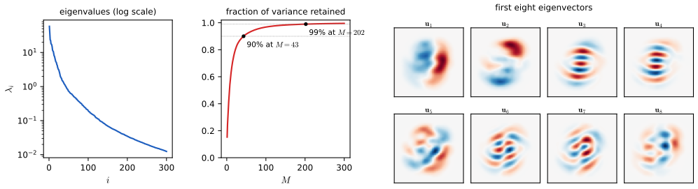
(Erratum. The book describes the MNIST digit as a \(64\times64\) image; MNIST images are \(28\times28\), as the book itself says in Figure 16.3. The enlargement above reconciles the two.) How strongly curved this manifold is can be measured with PCA itself: Figure 16.S1 in Section 16.1.5 shows that a linear subspace needs 43 dimensions to hold 90% of the variance of these three-parameter images.
The simplest model takes both the latent distribution and the conditional distribution to be Gaussian, with a mean that depends linearly on \(\bz\) (the linear-Gaussian model of Section 11.1.4 and Section 3.2.6). It leads to probabilistic PCA and factor analysis. We begin with the classical, non-probabilistic PCA.
16.1 Principal Component Analysis
See also the companion course, Section 12.1 (principal component analysis) and its PCA and probabilistic PCA demo.
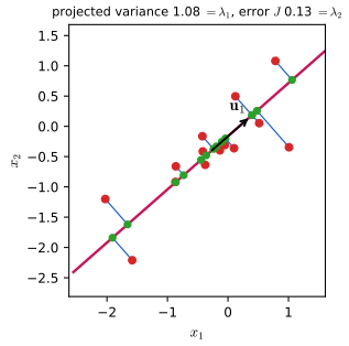
p. 497 Principal component analysis (PCA) projects the data orthogonally onto a lower-dimensional linear subspace, the principal subspace (Figure 16.2). It serves for dimensionality reduction, lossy compression, feature extraction and visualisation, and is also called the Kosambi–Karhunen–Loève transform. There are two classical definitions: the subspace on which the projected data have the largest variance (Hotelling, 1933), and the subspace that minimises the mean squared distance between the data and their projections (Pearson, 1901). They give the same answer.
16.1.1 Maximum variance formulation
See also the companion course, Section 12.1.1 and Filling the gap 12.1.
pp. 497–498 Let \(\bx_1,\dots,\bx_N\in\R^D\) be the data and fix \(M<D\). For \(M=1\) the subspace is the line spanned by a unit vector \(\bu_1\) (only its direction matters, so we impose \(\bu_1^\T\bu_1=1\)). Point \(\bx_n\) projects to the number \(\bu_1^\T\bx_n\), the projections have mean \(\bu_1^\T\bxbar\) with
\[ \bxbar=\frac1N\sum_{n=1}^N\bx_n, \tag{16.1} \]and variance
\[ \frac1N\sum_{n=1}^N\big\{\bu_1^\T\bx_n-\bu_1^\T\bxbar\big\}^2=\bu_1^\T\bS\bu_1, \tag{16.2} \] \[ \bS=\frac1N\sum_{n=1}^N(\bx_n-\bxbar)(\bx_n-\bxbar)^\T. \tag{16.3} \]To maximise \(\bu_1^\T\bS\bu_1\) under the constraint \(\bu_1^\T\bu_1=1\) we introduce a Lagrange multiplier \(\lambda_1\) (Appendix C of the book) and make stationary
\[ \bu_1^\T\bS\bu_1+\lambda_1\big(1-\bu_1^\T\bu_1\big). \tag{16.4} \]The gradient with respect to \(\bu_1\) is \(2\bS\bu_1-2\lambda_1\bu_1\), so
\[ \bS\bu_1=\lambda_1\bu_1, \tag{16.5} \]\(\bu_1\) is an eigenvector of \(\bS\), and multiplying by \(\bu_1^\T\),
\[ \bu_1^\T\bS\bu_1=\lambda_1 . \tag{16.6} \]The projected variance equals the eigenvalue, so the best \(\bu_1\) is the eigenvector of the largest eigenvalue: the first principal component.
Definition 16.1 (principal components and principal subspace) pp. 497–499
Let \(\bS\) be the sample covariance (16.3) with eigenvalues \(\lambda_1\ge\lambda_2\ge\dots\)
Result 16.1 (maximum variance in \(M\) dimensions) p. 498; Exercise 16.1
For every \(D\times M\) matrix \(\bQ\) with orthonormal columns, \(\Tr(\bQ^\T\bS\bQ)\)
Proof (short; the full argument is Result 12.2 of the companion course)
Write \(\bS=\sum_i\lambda_i\bu_i\bu_i^\T\). Then \(\Tr(\bQ^\T\bS\bQ)=\sum_i\lambda_ic_i\) with \(c_i=\Vert\bQ^\T\bu_i\Vert^2\). Each \(c_i\in[0,1]\) (the length of a projection of a unit vector), and \(\sum_ic_i=\Tr(\bQ^\T\bQ)=M\). Maximising \(\sum_i\lambda_ic_i\) over such weights puts weight 1 on the \(M\) largest \(\lambda_i\): any weight on a smaller eigenvalue can be moved to a larger one without decreasing the sum. Equality forces \(c_1=\dots=c_M=1\) when \(\lambda_M>\lambda_{M+1}\), i.e. \(\bu_1,\dots,\bu_M\in\span(\bQ)\). ∎
Filling the gap 16.1: the induction of Exercise 16.1, and what it does and does not prove p. 498, "easily shown using proof by induction"
The book builds the components one at a time. The induction step is short, but it proves a greedy statement; Result 16.1 is what shows the greedy answer is also the best \(M\)-dimensional subspace.
Derivation
Induction step. Suppose \(\bu_1,\dots,\bu_M\) are orthonormal eigenvectors of \(\bS\) for \(\lambda_1,\dots,\lambda_M\). We look for a unit vector \(\bu\) orthogonal to all of them that maximises \(\bu^\T\bS\bu\). With multipliers \(\lambda\) for \(\bu^\T\bu=1\) and \(\eta_j\) for \(\bu^\T\bu_j=0\), stationarity of \(\bu^\T\bS\bu+\lambda(1-\bu^\T\bu)\)
What it shows. The induction proves that choosing directions one after another, each maximising the variance among directions orthogonal to the earlier ones, yields \(\bu_1,\bu_2,\dots\). It does not by itself exclude an \(M\)-dimensional subspace that is not built greedily but keeps more total variance; the trace inequality of Result 16.1 closes that gap, and shows that the greedy and the joint optimum coincide for this objective.
Cost. A full eigendecomposition costs \(O(D^3)\). The power method or Lanczos iterations find the leading \(M\) eigenvectors at \(O(MD^2)\) per sweep once \(\bS\) is formed, and forming \(\bS\) costs \(O(ND^2)\); EM for PCA (Section 16.3.2) avoids \(\bS\) altogether at \(O(NDM)\) per iteration. ∎
Algorithm 16.1 (principal component analysis) p. 498
- Compute \(\bxbar\) (16.1) and \(\bS\) (16.3).
- Find the \(M\) leading eigenpairs \((\lambda_i,\bu_i)\) of \(\bS\) (or, if \(N<D\), use Result 16.4).
- Return the scores \(a_{ni}=\bu_i^\T(\bx_n-\bxbar)\), \(i=1,\dots,M\), and, if wanted, the reconstructions (16.20).
16.1.2 Minimum-error formulation
See also the companion course, Section 12.1.2, Filling the gap 12.2 and Result 12.3.
pp. 499–501 Take a complete orthonormal basis \(\{\bu_i\}_{i=1}^D\),
\[ \bu_i^\T\bu_j=\delta_{ij}. \tag{16.7} \]Every point has the exact expansion
\[ \bx_n=\sum_{i=1}^D\alpha_{ni}\bu_i, \tag{16.8} \]and taking inner products with \(\bu_j\) gives \(\alpha_{nj}=\bx_n^\T\bu_j\), so
\[ \bx_n=\sum_{i=1}^D\big(\bx_n^\T\bu_i\big)\bu_i . \tag{16.9} \]An \(M\)-dimensional approximation keeps \(M\) point-specific coefficients and replaces the others by constants shared by all points:
\[ \bxt_n=\sum_{i=1}^Mz_{ni}\bu_i+\sum_{i=M+1}^Db_i\bu_i , \tag{16.10} \]and we choose \(\{\bu_i\}\), \(\{z_{ni}\}\) and \(\{b_i\}\) to minimise the distortion
\[ J=\frac1N\sum_{n=1}^N\Vert\bx_n-\bxt_n\Vert^2 . \tag{16.11} \]The optimal coefficients are
\[ z_{nj}=\bx_n^\T\bu_j\quad(j\le M), \tag{16.12} \] \[ b_j=\bxbar^\T\bu_j\quad(j>M), \tag{16.13} \]so that
\[ \bx_n-\bxt_n=\sum_{i=M+1}^D\big\{(\bx_n-\bxbar)^\T\bu_i\big\}\bu_i , \tag{16.14} \]a vector orthogonal to the principal subspace, and
\[ J=\frac1N\sum_{n=1}^N\sum_{i=M+1}^D\big(\bx_n^\T\bu_i-\bxbar^\T\bu_i\big)^2=\sum_{i=M+1}^D\bu_i^\T\bS\bu_i . \tag{16.15} \]For \(D=2\), \(M=1\), minimising \(J=\bu_2^\T\bS\bu_2\) with a multiplier \(\lambda_2\),
\[ \widetilde J=\bu_2^\T\bS\bu_2+\lambda_2\big(1-\bu_2^\T\bu_2\big), \tag{16.16} \]gives \(\bS\bu_2=\lambda_2\bu_2\) and \(J=\lambda_2\), smallest when \(\bu_2\) belongs to the smaller eigenvalue. In general the minimum is attained with eigenvectors,
\[ \bS\bu_i=\lambda_i\bu_i , \tag{16.17} \]and its value is
\[ J=\sum_{i=M+1}^D\lambda_i , \tag{16.18} \]the sum of the eigenvalues orthogonal to the principal subspace. With \(M=D\) PCA is just a rotation of the axes. Canonical correlation analysis (Hotelling, 1936), mentioned on p. 501, applies the same idea to two sets of variables and leads to a generalised eigenproblem.
Result 16.2 (minimum error; the two definitions agree) pp. 499–501, (16.12)–(16.18); Exercise 16.2
Over all orthonormal bases and all coefficients, the minimum of (16.11) is \(\sum_{i>M}\lambda_i\), attained by the principal subspace of Result 16.1 with \(z_{nj}\) and \(b_j\) as in (16.12)–(16.13). Since \(J=\Tr\bS-\Tr(\bU_M^\T\bS\bU_M)\), minimising the error and maximising the retained variance are the same problem.
Filling the gap 16.2: from (16.10) to (16.15), and the general solution with a matrix of multipliers pp. 499–501; Exercise 16.2
Derivation
The coefficients. Subtract (16.10) from (16.9): \(\bx_n-\bxt_n\)
The basis. Since \(\sum_{i=1}^D\bu_i^\T\bS\bu_i=\Tr\bS\) for any orthonormal basis, \(J=\Tr\bS-\Tr(\bU_M^\T\bS\bU_M)\), and Result 16.1 gives the minimum \(\Tr\bS-\sum_{i\le M}\lambda_i\)
Exercise 16.2's route. Let \(\widehat\bU\) (\(D\times(D-M)\)) hold the discarded directions and \(\bH\) the multipliers of the constraints \(\widehat\bU^\T\widehat\bU=\bI\): \[ \widetilde J=\Tr\{\widehat\bU^\T\bS\widehat\bU\}+\Tr\{\bH(\bI-\widehat\bU^\T\widehat\bU)\}. \tag{16.87} \] Because \(\bI-\widehat\bU^\T\widehat\bU\) is symmetric, only the symmetric part of \(\bH\) enters, so \(\bH=\bH^\T\) without loss. The gradient \(2\bS\widehat\bU-\widehat\bU(\bH+\bH^\T)\) vanishes when \(\bS\widehat\bU=\widehat\bU\bH\). Multiplying by \(\widehat\bU^\T\) gives \(\bH=\widehat\bU^\T\bS\widehat\bU\). Diagonalise \(\bH=\bPsi\Lambda\bPsi^\T\) with \(\bPsi\) orthogonal; then \(\widetilde\bU=\widehat\bU\bPsi\) satisfies \(\bS\widetilde\bU=\widetilde\bU\Lambda\), so its columns are orthonormal eigenvectors of \(\bS\), and \(J=\Tr\bH=\Tr\Lambda\) is the sum of their eigenvalues. Every stationary point therefore spans an invariant subspace of \(\bS\), its value is a sum of \(D-M\) eigenvalues, and the minimum takes the \(D-M\) smallest. A rotated basis of the same subspace (non-diagonal \(\bH\)) gives the same \(J\), as a direct computation confirms. ∎
16.1.3 Data compression
See also the companion course, Section 12.1.3 (applications of PCA).
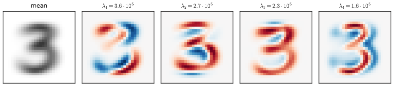
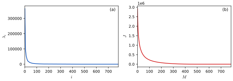
pp. 501–502 Each eigenvector is a vector in pixel space, so it can be displayed as an image. Figure 16.3 shows the mean and the first four eigenvectors of 6000 MNIST threes, Figure 16.4 the whole spectrum and the distortion \(J(M)\).
Substituting (16.12) and (16.13) into (16.10), the approximation of a data point is
\[ \bxt_n=\sum_{i=1}^M(\bx_n^\T\bu_i)\bu_i+\sum_{i=M+1}^D(\bxbar^\T\bu_i)\bu_i \tag{16.19} \] \[ \phantom{\bxt_n}=\bxbar+\sum_{i=1}^M\big(\bx_n^\T\bu_i-\bxbar^\T\bu_i\big)\bu_i , \tag{16.20} \]where we used completeness in the form
\[ \bxbar=\sum_{i=1}^D\big(\bxbar^\T\bu_i\big)\bu_i . \tag{16.21} \]Each point is stored as \(M\) numbers \(a_{ni}=(\bx_n-\bxbar)^\T\bu_i\) instead of \(D\); the mean and the \(M\) eigenvectors are stored once.
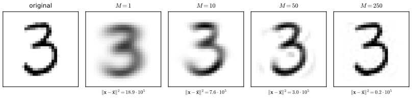
Filling the gap 16.3: the error of one image, and why reconstruction error is a weak novelty score pp. 501–503, (16.18)–(16.21)
(16.18) is an average over the training set. For a single image, and for an image that is not a three, the error behaves differently.
Derivation
One image. Let \(\bx\) be any image with scores \(a_i=\bu_i^\T(\bx-\bxbar)\), \(i=1,\dots,D\). By (16.14) and orthonormality,
\[ \Vert\bx-\bxt\Vert^2=\sum_{i>M}a_i^2=\Vert\bx-\bxbar\Vert^2-\sum_{i\le M}a_i^2 , \]
a decreasing function of \(M\) that reaches 0 at \(M=D\). Averaging over the training images, \(\frac1N\sum_na_{ni}^2=\bu_i^\T\bS\bu_i\)
A different digit. For an image from another class, the scores along the leading eigenvectors are not where they would be for a three, and \(\Vert\bx-\bxbar\Vert^2\) is larger. In the demo, a 7 seen through the eigenvectors of threes has, at \(M=20\), an error 2.2 times the training average \(J(20)\), while test threes have 0.56 to 0.91 times. But one test three, written unusually, also has 2.1 times, and as \(M\to D\) every image is rebuilt exactly. Reconstruction error measures only the distance to the subspace; a probabilistic model (Section 16.2) adds how far along the subspace the point lies, in units of \(\sqrt{\lambda_i}\). The probabilistic PCA log density of the 7 is \(-5.61\) nats per pixel against \(-4.8\) to \(-5.0\) for most test threes (and \(-5.58\) for the unusual one). ∎
16.1.4 Data whitening
See also the companion course, Result 12.4 (whitening) and the whitening view of its PCA demo.
pp. 502–504 PCA is also a pre-processing step. Variables in different units or with very different spreads (in the Old Faithful data the waiting time is about twenty times the eruption duration) are often standardised to zero mean and unit variance; the covariance of the standardised data is the correlation matrix
\[ \rho_{ij}=\frac1N\sum_{n=1}^N\frac{(x_{ni}-\overline x_i)}{\sigma_i}\frac{(x_{nj}-\overline x_j)}{\sigma_j}, \tag{16.22} \]with \(\rho_{ij}=\pm1\) for perfectly (positively or negatively) correlated variables and 0 for uncorrelated ones. PCA goes further and removes the correlations. Collect the eigenvectors as columns of an orthogonal \(\bU\) and the eigenvalues in a diagonal \(\bL\), so that
\[ \bS\bU=\bU\bL , \tag{16.23} \]and define
\[ \by_n=\bL^{-1/2}\bU^\T(\bx_n-\bxbar). \tag{16.24} \]Then \(\{\by_n\}\) has zero mean and covariance
\[ \frac1N\sum_{n=1}^N\by_n\by_n^\T=\bL^{-1/2}\bU^\T\bS\bU\bL^{-1/2}=\bL^{-1/2}\bL\bL^{-1/2}=\bI . \tag{16.25} \]This is whitening or sphering (Figure 16.6). It needs all \(\lambda_i>0\).
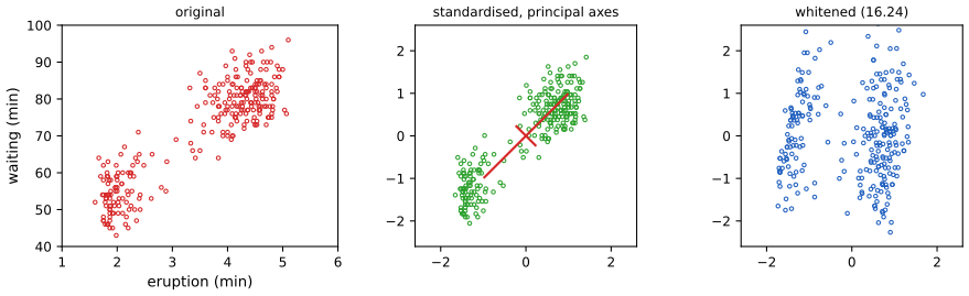
Result 16.3 (whitening and its non-uniqueness) pp. 503–504, (16.23)–(16.25)
If \(\bS\) is non-singular, \(\by_n=\bL^{-1/2}\bU^\T(\bx_n-\bxbar)\) has sample mean \(\bzero\) and sample covariance \(\bI\). For any orthogonal \(\bR\), \(\bR\by_n\) is white as well, and every linear map \(\bA\) with \(\bA\bS\bA^\T=\bI\) has the form \(\bA=\bR\bL^{-1/2}\bU^\T\).
Proof
The mean is \(\bL^{-1/2}\bU^\T(\bxbar-\bxbar)=\bzero\) and the covariance is (16.25). For \(\bR\by_n\) the covariance is \(\bR\bI\bR^\T=\bI\). Conversely, if \(\bA\bS\bA^\T=\bI\), put \(\bR=\bA\bU\bL^{1/2}\); then \(\bR\bR^\T=\bA\bU\bL\bU^\T\bA^\T\)
The rotation \(\bR\) is exactly what second-order statistics cannot determine, and what independent component analysis (Section 16.2.5) recovers from higher-order statistics.
16.1.5 High-dimensional data
See also the companion course, Section 12.1.4 and Result 12.5.
pp. 504–505 When \(N<D\) (a few hundred images of millions of pixels) the \(N\) centred points span at most \(N-1\) dimensions, at least \(D-N+1\) eigenvalues are zero, and an \(O(D^3)\) eigensolver is wasteful. Let \(\bX\) be the \(N\times D\) centred data matrix with rows \((\bx_n-\bxbar)^\T\), so \(\bS=N^{-1}\bX^\T\bX\) and
\[ \frac1N\bX^\T\bX\bu_i=\lambda_i\bu_i . \tag{16.26} \]Multiplying by \(\bX\),
\[ \frac1N\bX\bX^\T(\bX\bu_i)=\lambda_i(\bX\bu_i), \tag{16.27} \]so \(\bv_i=\bX\bu_i\) solves the \(N\times N\) problem
\[ \frac1N\bX\bX^\T\bv_i=\lambda_i\bv_i . \tag{16.28} \]Conversely, multiplying (16.28) by \(\bX^\T\),
\[ \Big(\frac1N\bX^\T\bX\Big)(\bX^\T\bv_i)=\lambda_i(\bX^\T\bv_i), \tag{16.29} \]and normalising (for unit \(\bv_i\)),
\[ \bu_i=\frac1{(N\lambda_i)^{1/2}}\bX^\T\bv_i . \tag{16.30} \]Result 16.4 (PCA through the \(N\times N\) matrix) pp. 504–505, (16.26)–(16.30); Exercise 16.3
- \(\bX^\T\bX/N\) and \(\bX\bX^\T/N\) have the same non-zero eigenvalues, with the same multiplicities.
- Since the rows of the centred \(\bX\) sum to zero, \(\operatorname{rank}\bX\le\min(N-1,D)\); so \(\bS\) has at least \(D-N+1\) zero eigenvalues when \(N\le D\), and \(\bX\bX^\T\) has the eigenvector \(\mathbf 1\) with eigenvalue 0.
- If \(\bv_i\) is a unit eigenvector of \(\bX\bX^\T/N\) with \(\lambda_i>0\), (16.30) is a unit eigenvector of \(\bS\). The cost is \(O(N^2D)\) to form \(\bX\bX^\T\), \(O(N^3)\) to diagonalise it and \(O(NDM)\) to map back.
Proof (short; full version in Result 12.5)
(1) From the singular value decomposition \(\bX=\sum_k s_k\mathbf a_k\mathbf b_k^\T\): \(\bX^\T\bX\)
Applied to 60 threes: 725 eigenvalues of \(\bS\) vanish, and the \(60\times60\) route reproduces the non-zero eigenvalues and unit eigenvectors to \(10^{-8}\).
The \(N\times N\) route is what makes PCA of the \(10\,000\)-pixel images of Figure 16.1 cheap. It answers a question raised in the introduction: how linear is the three-parameter manifold?
16.2 Probabilistic Latent Variables
See also the companion course, Section 12.2 (probabilistic PCA).
p. 506 The scores \(z_{nj}\) of (16.12) are deterministic latent variables. Recasting PCA as the maximum likelihood solution of a probabilistic latent variable model (Tipping and Bishop, 1997, 1999; Roweis, 1998) brings: a Gaussian whose number of parameters grows only linearly with \(D\) yet captures the main correlations; an EM algorithm that never forms \(\bS\); a principled treatment of missing values; mixtures of PCA models; a likelihood for comparing with other density models (plain PCA gives a small reconstruction cost to points near the subspace however far they are from the data); class-conditional densities for classification; sampling; and Bayesian versions that choose \(M\) (Bishop, 2006; companion Section 12.2.3).
16.2.1 Generative model
See also the companion course, Definition 12.2, and the linear-Gaussian model of Section 11.1.4 of these notes (Gaussian variables in graphical models).
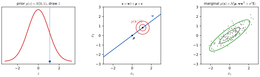
pp. 506–507 Probabilistic PCA is a linear-Gaussian model with
\[ p(\bz)=\N(\bz\given\bzero,\bI), \tag{16.31} \] \[ p(\bx\given\bz)=\N(\bx\given\bW\bz+\bmu,\sigma^2\bI), \tag{16.32} \]where \(\bW\) is \(D\times M\) and \(\bmu\in\R^D\). The covariance of \(p(\bx\given\bz)\) is diagonal, so the components of \(\bx\) are independent given \(\bz\): a naive Bayes structure (Section 11.2.3; Exercise 16.7). Equivalently,
\[ \bx=\bW\bz+\bmu+\beps,\qquad\beps\sim\N(\bzero,\sigma^2\bI)\ \text{independent of }\bz. \tag{16.33} \]The map goes from latent space to data space, the reverse of the projection view of Section 16.1; Bayes' theorem will supply the other direction. A general Gaussian prior \(\N(\bz\given\mathbf m,\Sig)\) gives nothing new (Exercise 16.4).
Definition 16.2 (probabilistic PCA) pp. 506–507, (16.31)–(16.33)
Parameters \(\bW\in\R^{D\times M}\), \(\bmu\in\R^D\), \(\sigma^2>0\). Data are generated by drawing \(\bz\sim\N(\bzero,\bI_M)\) and then \(\bx\sim\N(\bW\bz+\bmu,\sigma^2\bI_D)\), independently for each data point (Figure 16.8, a plate diagram, not reproduced).
16.2.2 Likelihood function
pp. 507–509 The marginal of \(\bx\) is
\[ p(\bx)=\int p(\bx\given\bz)p(\bz)\,\d\bz \tag{16.34} \]and, the model being linear-Gaussian,
\[ p(\bx)=\N(\bx\given\bmu,\bC), \tag{16.35} \] \[ \bC=\bW\bW^\T+\sigma^2\bI . \tag{16.36} \]Directly from (16.33), using the independence of \(\bz\) and \(\beps\):
\[ \E[\bx]=\E[\bW\bz+\bmu+\beps]=\bmu , \tag{16.37} \] \[ \cov[\bx]=\E\big[(\bW\bz+\beps)(\bW\bz+\beps)^\T\big]=\E\big[\bW\bz\bz^\T\bW^\T\big]+\E[\beps\beps^\T] \tag{16.38} \] \[ \phantom{\cov[\bx]}=\bW\bW^\T+\sigma^2\bI . \tag{16.39} \]The density is like Gaussian ink sprayed from a can moving along the principal subspace. It does not identify \(\bW\): for any orthogonal \(\bR\), \(\widetilde\bW=\bW\bR\) gives
\[ \widetilde\bW\widetilde\bW^\T=\bW\bR\bR^\T\bW^\T=\bW\bW^\T , \tag{16.40} \]a rotation of latent space. Evaluating the density needs \(\bC^{-1}\); by the Woodbury identity
\[ \bC^{-1}=\sigma^{-2}\bI-\sigma^{-2}\bW\bM^{-1}\bW^\T , \tag{16.41} \] \[ \bM=\bW^\T\bW+\sigma^2\bI , \tag{16.42} \]which costs \(O(M^3)\) (plus \(O(DM^2)\) to form \(\bM\)) instead of \(O(D^3)\). The posterior, from the linear-Gaussian result (3.100) of Section 3.2.6, is
\[ p(\bz\given\bx)=\N\big(\bz\given\bM^{-1}\bW^\T(\bx-\bmu),\ \sigma^2\bM^{-1}\big); \tag{16.43} \]its mean depends on \(\bx\), its covariance does not.
Result 16.5 (marginal and posterior of probabilistic PCA) pp. 507–509, (16.35)–(16.43); Exercises 16.4, 16.6, 16.8
- \(p(\bx)=\N(\bmu,\bW\bW^\T+\sigma^2\bI)\), invariant under \(\bW\mapsto\bW\bR\) for orthogonal \(\bR\).
- \(\bC^{-1}\) is given by (16.41), and \(|\bC|=\sigma^{2(D-M)}|\bM|\).
- \(p(\bz\given\bx)\) is (16.43).
- A prior \(\N(\mathbf m,\Sig)\) on \(\bz\) gives the same family of marginals, with \(\bW'=\bW\Sig^{1/2}\) and \(\bmu'=\bmu+\bW\mathbf m\).
Proof (short; full version in Result 12.6 of the companion course)
(1) \((\bz,\beps)\) is jointly Gaussian, so \(\bx\), an affine function of it, is Gaussian with the moments (16.37)–(16.39). (2) Woodbury: \((\sigma^2\bI+\bW\bW^\T)^{-1}\)
16.2.3 Maximum likelihood
See also the companion course, Section 12.2.1 and Result 12.8 (the full Tipping–Bishop analysis).
pp. 509–513 For data \(\bX=\{\bx_n\}\) the log likelihood is
\[ \ln p(\bX\given\bmu,\bW,\sigma^2)=\sum_{n=1}^N\ln p(\bx_n\given\bW,\bmu,\sigma^2)=-\frac{ND}2\ln(2\pi)-\frac N2\ln|\bC|-\frac12\sum_{n=1}^N(\bx_n-\bmu)^\T\bC^{-1}(\bx_n-\bmu). \tag{16.44} \]It is a concave quadratic in \(\bmu\) (Hessian \(-N\bC^{-1}\); Exercises 16.9, 16.10), maximised by \(\bmu=\bxbar\), after which
\[ \ln p(\bX\given\bW,\bmu,\sigma^2)=-\frac N2\Big\{D\ln(2\pi)+\ln|\bC|+\Tr\big(\bC^{-1}\bS\big)\Big\}. \tag{16.45} \]Tipping and Bishop (1999) showed that all stationary points in \(\bW\) have the form
\[ \bW_{\rm ML}=\bU_M(\bL_M-\sigma^2\bI)^{1/2}\bR , \tag{16.46} \]where the columns of \(\bU_M\) are any \(M\) eigenvectors of \(\bS\), \(\bL_M\) holds their eigenvalues and \(\bR\) is any orthogonal matrix; the maximum takes the \(M\) leading eigenvectors (all other choices are saddle points), and then
\[ \sigma^2_{\rm ML}=\frac1{D-M}\sum_{i=M+1}^D\lambda_i , \tag{16.47} \]the average variance of the discarded directions. With \(\bR=\bI\), the columns of \(\bW\) are the eigenvectors scaled by \((\lambda_i-\sigma^2)^{1/2}\). (Erratum. The book says "scaled by the variance parameters \(\lambda_i-\sigma^2\)"; the scale factor is the square root, so that the variance contributed along \(\bu_i\) is \(\lambda_i-\sigma^2\).) Along a retained eigenvector the model variance is \(\bu_i^\T\bC\bu_i\)
Result 16.6 (maximum likelihood probabilistic PCA; Tipping and Bishop, 1999) pp. 510–511, (16.45)–(16.48)
Assume \(\bS\) is non-singular. Then:
- \(\bW\) is a stationary point of (16.45) for fixed \(\sigma^2\) iff \(\bS\bC^{-1}\bW=\bW\), iff \(\bW=\bU_q(\bL_q-\sigma^2\bI)^{1/2}\bR\) for some set \(q\) of eigenvectors with \(\lambda_i\ge\sigma^2\) (columns for which \(\lambda_i=\sigma^2\) are zero, so \(\bW\) may have rank below \(M\)).
- For a given set of \(M\) retained eigenvalues, the optimal \(\sigma^2\) is the mean of the others, (16.47).
- If a retained eigenvalue \(\lambda_r\) is smaller than a discarded one \(\lambda_d\), the stationary point is a saddle: turning the column for \(\bu_r\) towards \(\bu_d\) increases the likelihood. The global maximum therefore retains \(\lambda_1,\dots,\lambda_M\).
Filling the gap 16.4: why the eigenvectors appear, why only the principal ones give the maximum p. 510, "It was shown by Tipping and Bishop (1999)"
The book quotes the result. Here is a self-contained proof of each part; the companion course's Result 12.8 gives an alternative presentation.
Derivation
Gradient. With \(\d\ln|\bC|=\Tr(\bC^{-1}\d\bC)\), \(\d\bC^{-1}=-\bC^{-1}\d\bC\,\bC^{-1}\) and \(\d\bC=\d\bW\,\bW^\T+\bW\,\d\bW^\T\), \[ \frac{\partial}{\partial\bW}\ln p=N\big(\bC^{-1}\bS\bC^{-1}\bW-\bC^{-1}\bW\big), \] which vanishes iff \(\bS\bC^{-1}\bW=\bW\) (multiply by \(\bC\)).
Solving the stationarity equation. Write the thin SVD \(\bW=\mathbf V\mathbf K\bR^\T\) (\(\mathbf V\): \(D\times M\) orthonormal columns, \(\mathbf K=\diag(k_j)\ge0\)). Then \(\bC\mathbf V\)
The noise variance. At such a point \(\bC\) has eigenvectors \(\bu_1,\dots,\bu_D\), with eigenvalue \(\lambda_i\) for the retained ones and \(\sigma^2\) for the others. So \(\ln|\bC|\)
Saddles. Let \(\lambda_r\) be retained and \(\lambda_d>\lambda_r\) discarded, with \(\lambda_r>\sigma^2\). Replace the column \(k_r\bu_r\) by \(k_r(\cos\epsilon\,\bu_r\)
Back to data space. pp. 511–512 Probabilistic PCA maps latent to data space; for visualisation or compression we reverse it with Bayes' theorem. A point \(\bx\) is summarised by its posterior mean
\[ \E[\bz\given\bx]=\bM^{-1}\bW_{\rm ML}^\T(\bx-\bxbar), \tag{16.49} \]which maps back to
\[ \bW\E[\bz\given\bx]+\bmu \tag{16.50} \](a regularised linear regression, as in Section 4.1.6), and by the \(\bx\)-independent posterior covariance \(\sigma^2\bM^{-1}\). As \(\sigma^2\to0\) the posterior mean becomes
\[ (\bW_{\rm ML}^\T\bW_{\rm ML})^{-1}\bW_{\rm ML}^\T(\bx-\bxbar), \tag{16.51} \]the orthogonal projection of standard PCA (with zero posterior covariance: the density becomes singular). For \(\sigma^2>0\) the latent projection is shrunk towards the origin.
Result 16.7 (the posterior mean shrinks; the best reconstruction undoes it) p. 512, (16.49)–(16.51); Exercises 16.11–16.13
At the ML solution with \(\bR=\bI\), let \(a_j=\bu_j^\T(\bx-\bxbar)\). Then
\[ \E[z_j\given\bx]=\frac{(\lambda_j-\sigma^2)^{1/2}}{\lambda_j}a_j,\qquad\text{orthogonal projection (16.51): }\ \frac{a_j}{(\lambda_j-\sigma^2)^{1/2}} , \]
so the posterior mean is the projection multiplied by \((\lambda_j-\sigma^2)/\lambda_j\in(0,1)\), tending to 1 as \(\sigma^2\to0\). The reconstruction (16.50) is \(\bxbar\)
Proof (short; full version in Result 12.9)
With \(\bW=\bU_M(\bL_M-\sigma^2\bI)^{1/2}\): \(\bW^\T\bW=\bL_M-\sigma^2\bI\), \(\bM=\bL_M\), \(\bW^\T(\bx-\bxbar)\)
Counting parameters. pp. 512–513 A full covariance has \(D(D+1)/2\) parameters, a diagonal one \(D\) but no correlations. Probabilistic PCA sits between them: \(\bW\) and \(\sigma^2\) have \(DM+1\) entries, of which a rotation \(\bR\) (\(M(M-1)/2\) parameters) is redundant, so the covariance has
\[ DM+1-M(M-1)/2 \tag{16.52} \]degrees of freedom: linear in \(D\) for fixed \(M\). With \(M=D-1\) this is \(D(D+1)/2\) (a full covariance: \(D-1\) directions from \(\bW\), the last from \(\sigma^2\)); with \(M=0\) it is 1 (isotropic).
Result 16.8 (degrees of freedom of the PPCA and factor analysis covariances) pp. 512–513, (16.52); Exercises 16.14, 16.15
At a generic \((\bW,\sigma^2)\) the Jacobian of the map \((\bW,\sigma^2)\mapsto\bC\) has rank \(DM+1-M(M-1)/2\); for factor analysis \((\bW,\bPsi)\mapsto\bW\bW^\T+\bPsi\) it has rank \(DM+D-M(M-1)/2\) (when this does not exceed \(D(D+1)/2\)).
Proof
The orthogonal \(M\times M\) matrices form a manifold of dimension \(M(M-1)/2\): the first column is a unit vector (\(M-1\) free parameters), the second a unit vector orthogonal to it (\(M-2\)), and so on, \(\sum_{k=1}^{M-1}k=M(M-1)/2\); equivalently, its tangent space at \(\bI\) is the space of antisymmetric matrices. The fibre \(\{\bW\bR\}\) of a full-rank \(\bW\) has exactly this dimension, and no other changes of \(\bW\) leave \(\bW\bW^\T\) fixed (if \(\bW\bW^\T=\bW'\bW'^\T\) with \(\bW\) of full column rank, then \(\bW'=\bW\bR\) for an orthogonal \(\bR\)). So the image has dimension \(DM+1-M(M-1)/2\). For \(M=D-1\): \(D(D-1)+1-(D-1)(D-2)/2\)
16.2.4 Factor analysis
See also the companion course, Section 12.2.4, Result 12.13 and its Bayesian PCA and factor analysis demo.
pp. 513–514 Factor analysis differs from probabilistic PCA only in the noise:
\[ p(\bx\given\bz)=\N(\bx\given\bW\bz+\bmu,\bPsi),\qquad\bPsi\ \text{diagonal}. \tag{16.53} \]The variables are still independent given \(\bz\); \(\bPsi\) holds the variance specific to each variable (the uniquenesses) and the columns of \(\bW\) (the factor loadings) the shared covariance. The marginal is \(\N(\bx\given\bmu,\bC)\) with
\[ \bC=\bW\bW^\T+\bPsi . \tag{16.54} \]Lawley (1953) and Anderson (1963) found the stationary points for \(\bPsi=\sigma^2\bI\); Tipping and Bishop (1999) identified the maximum. Unlike PPCA, factor analysis has no closed-form maximum likelihood solution (Section 16.3.3 gives EM). The model is again invariant to rotations of \(\bz\), which made attempts to interpret individual factors controversial; to remove the rotation one needs a non-Gaussian latent distribution (Section 16.2.5).
Definition 16.3 (factor analysis) p. 513, (16.53)–(16.54)
As Definition 16.2 but with \(p(\bx\given\bz)=\N(\bW\bz+\bmu,\bPsi)\), \(\bPsi=\diag(\psi_1,\dots,\psi_D)\), \(\psi_i>0\).
Result 16.9 (how the fits transform) pp. 513–514; Exercises 16.16, 16.17
Let a model have \(p(\bx\given\bz)=\N(\bW\bz+\bmu,\bPhi)\) with \(\bPhi\) in some class, and let \(\bA\) be non-singular. If \((\bmu,\bW,\bPhi)\) maximises the likelihood of \(\{\bx_n\}\), then \((\bA\bmu,\bA\bW,\bA\bPhi\bA^\T)\) maximises the likelihood of \(\{\bA\bx_n\}\), provided \(\bPhi\mapsto\bA\bPhi\bA^\T\) maps the class onto itself. This holds for factor analysis (diagonal \(\bPhi\)) with diagonal \(\bA\) (rescaling each variable), and for PPCA (\(\bPhi=\sigma^2\bI\)) with orthogonal \(\bA\) (rotating the axes). Both models are invariant under \(\bW\mapsto\bW\bR\).
Proof (short; full version in Result 12.13)
If \(\bx\sim\N(\bmu,\bW\bW^\T+\bPhi)\) then \(\bA\bx\sim\N(\bA\bmu,(\bA\bW)(\bA\bW)^\T\)
16.2.5 Independent component analysis
See also the companion course, Section 12.4.1, Definition 12.4 and Result 12.16.
pp. 514–515 Keep the linear map but make the latent distribution non-Gaussian and factorised:
\[ p(\bz)=\prod_{j=1}^Mp(z_j). \tag{16.55} \]The motivating problem is blind source separation (Cardoso, 1998): two people talk at once and two microphones record different linear combinations of their voices (ignoring delays and echoes). Neither the voices nor the mixing coefficients are observed; if the mixing is learned and is invertible, it can be undone. Treating the time samples as independent (MacKay, 2003), the model has two latent sources and two observed signals, \(\bx=\bA\bz\), with no noise term: since \(M=D\), the distribution of \(\bx\) is non-singular. The log likelihood is a function of the mixing coefficients and can be maximised by gradient methods. This needs non-Gaussian sources: with a Gaussian \(p(\bz)\), \(\bW\) and \(\bW\bR\) give the same likelihood (16.40), and decorrelating the data (PCA) gives independence only for Gaussians, since zero correlation is necessary but not sufficient for independence. A common choice is
\[ p(z_j)=\frac1{\pi\cosh(z_j)}=\frac2{\pi(e^{z_j}+e^{-z_j})}, \tag{16.56} \]whose tails, \(\propto e^{-|z|}\), are heavier than a Gaussian's; it has variance \(\pi^2/4\) and excess kurtosis 2. The original ICA algorithm maximised information transfer (Bell and Sejnowski, 1995); the probabilistic view leads to extensions such as independent factor analysis (Attias, 1999), with noise, unequal numbers of sources and sensors, and mixture-of-Gaussian sources.
Definition 16.4 (noise-free square ICA) p. 514
Sources \(\bz\in\R^D\) with independent components, \(p(\bz)=\prod_jp_j(z_j)\); observations \(\bx=\bA\bz\) with \(\bA\) a non-singular \(D\times D\) mixing matrix. The unmixing matrix is \(\bW=\bA^{-1}\) with rows \(\bw_j^\T\), so \(z_j=\bw_j^\T\bx\). We write \(\varphi_j=-(\ln p_j)'\) (the score with the sign changed): \(\varphi(z)=\tanh z\) for (16.56).
Result 16.10 (the ICA likelihood, its gradient, and when it identifies the sources) pp. 514–515
- \(\displaystyle\ln p(\bX\given\bW)\)
\({}=N\ln|\det\bW|\) \({}+\sum_{n=1}^N\sum_{j=1}^D\ln p_j(\bw_j^\T\bx_n)\), with gradient \(N\bW^{-\T}\) \({}-\sum_n\boldsymbol\varphi(\bz_n)\bx_n^\T\) and natural gradient \(\big(N\bI\) \({}-\sum_n\boldsymbol\varphi(\bz_n)\bz_n^\T\big)\bW\) (Amari, Cichocki and Yang, 1996). - If the sources are Gaussian, \(p(\bx)=\N(\bzero,\bA\bA^\T)\) depends on \(\bA\) only through \(\bA\bA^\T\): \(\bA\) and \(\bA\bR\) cannot be distinguished. If at most one source is Gaussian, \(\bA\) is identifiable up to permutation and scaling of its columns (Comon, 1994, from the Darmois–Skitovich theorem).
- On whitened data with unit-variance sources, rotations \(\bW=\bR(\theta)\) and the light-tailed prior \(p(z)\propto e^{-z^4/4}\):
\[ \frac1N\ln p\to\const+\frac{\kappa_1+\kappa_2}{8}\sin^2 2\phi ,\qquad\phi=\text{angle between }\bR(\theta)\text{ and the separating rotation}, \]
where \(\kappa_j=\E z_j^4-3\) are the sources' excess kurtoses. With the sech prior (16.56) the same calculation to fourth order gives \(\const\)
\({}-\frac{\kappa_1+\kappa_2}{24}\sin^22\phi\). So a prior that is heavier-tailed than a Gaussian recovers super-Gaussian sources (\(\kappa>0\)), and a lighter-tailed one recovers sub-Gaussian sources (\(\kappa<0\)); with the wrong one, the separating rotation is a minimum of the likelihood and the maximum lies \(45^\circ\) away.
Filling the gap 16.5: the ICA likelihood by a change of variables, and why the prior's tails must match the sources pp. 514–515, "the log likelihood can be maximized using gradient-based optimization"; (16.56)
The book describes the model and the choice (16.56) in words. Here are the likelihood, its gradient, the natural gradient, the non-identifiability, and the condition under which (16.56) actually works, which the book does not discuss and which decides success or failure in practice.
Derivation
Likelihood. \(\bx=\bA\bz\) is an invertible linear change of variables, so by (16.78) \(p(\bx)=p_{\bz}(\bW\bx)\,|\det\bW|\) with \(\bW=\bA^{-1}\). Independence gives \(\ln p(\bx)\)
Gradient. \(\partial\ln|\det\bW|/\partial\bW\)
Gaussian sources. If \(p(\bz)=\N(\bzero,\bI)\), \(p(\bx)=\N(\bzero,\bA\bA^\T)\), and \(\bA\bR\) gives the same. More generally, for whitened data \(\by\) and a Gaussian prior, \(\sum_j\ln p((\bR\by)_j)\)
Whitening reduces the search to a rotation. Whiten first, \(\by=\mathbf V\bx\) (Result 16.3). If the sources have unit variance, \(\by=(\mathbf V\bA)\bz\) is white, so \(\mathbf V\bA\) is orthogonal, and the unmixing matrix of \(\by\) is a rotation (times a sign or permutation). With \(\bW=\bR\) orthogonal the term \(\ln|\det\bW|=0\), and the average log likelihood is \(\ell(\bR)\)
The sign of the kurtosis. Take \(D=2\) and write the estimates as a rotation by \(\phi\) of the true sources, \(\hat z_1=c\,s_1+s\,s_2\), \(\hat z_2=-s\,s_1+c\,s_2\) (\(c=\cos\phi\), \(s=\sin\phi\)), with independent, zero-mean, unit-variance sources and \(m_j=\E s_j^4=3+\kappa_j\). Odd moments of a single source may be non-zero, but every cross term containing an odd power of an independent zero-mean factor vanishes, so
\[ \E\hat z_1^4=c^4m_1+s^4m_2+6c^2s^2,\qquad\E\hat z_2^4=s^4m_1+c^4m_2+6c^2s^2 , \]
\[ \E\hat z_1^4+\E\hat z_2^4=(1-2c^2s^2)(m_1+m_2)+12c^2s^2=(m_1+m_2)-\tfrac12\sin^22\phi\,(\kappa_1+\kappa_2), \]
using \(c^4+s^4=1-2c^2s^2\) and \(2c^2s^2=\frac12\sin^22\phi\). For the light-tailed prior, \(\ln p(z)=-z^4/4-\ln c_4\) exactly, so \(\ell\)
Consequences. (16.56) is the right default for speech and many natural signals, which are super-Gaussian. For sub-Gaussian sources (uniform noise, sinusoids, sawtooth waves) it converges to the most mixed rotation. Practical algorithms either choose the nonlinearity per source from the sign of an estimated kurtosis ("extended infomax", Lee, Girolami and Sejnowski, 1999) or learn flexible source densities (Attias, 1999). ∎
Algorithm 16.2 (maximum likelihood ICA by natural gradient) pp. 514–515
- Centre and whiten the data, \(\by_n=\bL^{-1/2}\bU^\T(\bx_n-\bxbar)\) (16.24).
- Start from \(\bW=\bI\) (or any rotation). Repeat: \(\bz_n=\bW\by_n\); \(\bW\leftarrow\bW+\eta\big(\bI-\frac1N\sum_n\boldsymbol\varphi(\bz_n)\bz_n^\T\big)\bW\), with \(\varphi=\tanh\) for (16.56).
- The sources are recovered up to order, sign and scale; the full unmixing matrix for \(\bx\) is \(\bW\bL^{-1/2}\bU^\T\).

16.2.6 Kalman filters
See also the companion course, Section 13.3 (linear dynamical systems), Section 13.3.1 (inference) and its Kalman filter demo.
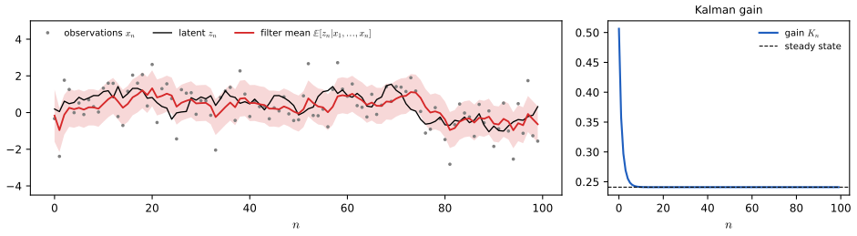
pp. 515–516 For sequences the i.i.d. assumption fails. As the hidden Markov model chains discrete latent variables, a linear dynamical system chains continuous ones (Figure 16.9, a drawing not reproduced): each \(p(\bx_n\given\bz_n)\) is a linear-Gaussian latent variable model, and the latent variables form a Markov chain with linear-Gaussian transitions \(p(\bz_n\given\bz_{n-1})\). The parameters are shared across time steps. The book calls the model a Kalman filter (Zarchan and Musoff, 2005); strictly, the Kalman filter is the recursive algorithm that computes \(p(\bz_n\given\bx_1,\dots,\bx_n)\) in this model. Hidden Markov models and linear dynamical systems were developed separately and share the same graph; the book returns to i.i.d. data after this section.
Definition 16.5 (linear dynamical system) pp. 515–516
\(\bz_1\sim\N(\bmu_0,\mathbf P_0)\); \(\bz_n=\bA\bz_{n-1}+\mathbf w_n\), \(\mathbf w_n\sim\N(\bzero,\boldsymbol\Gamma)\); \(\bx_n=\bC\bz_n+\mathbf v_n\), \(\mathbf v_n\sim\N(\bzero,\Sig)\); all noises independent. (In this subsection \(\bA\) and \(\bC\) are the transition and emission matrices.)
Result 16.11 (the Kalman filter and the likelihood) pp. 515–516
\(p(\bz_n\given\bx_1,\dots,\bx_n)\)
Filling the gap 16.6: the filter recursions from two linear-Gaussian operations p. 516, "efficient algorithms that involve propagating messages around the graph"
Derivation
Induction on \(n\). Suppose \(p(\bz_{n-1}\given\bx_{1:n-1})\)
Steady state. For the scalar model of Figure 16.S3 (\(z_n=az_{n-1}+w\), \(x_n=z_n+v\)), the predictive variance obeys the Riccati recursion \(P^-_{n+1}=a^2P^-_nr/(P^-_n+r)+q\), a contraction whose fixed point solves \(P^2+(r-a^2r-q)P-qr=0\); the gain converges to \(P/(P+r)\). With \(a=0.95\), \(q=0.1\), \(r=1\) the steady gain is 0.241. The filter is confirmed against brute-force conditioning of the joint Gaussian of the whole sequence (mean and variance at \(n=25\), and the total log likelihood, to \(10^{-9}\)). Full derivations, the smoother and EM are in the companion course, Section 13.3.1 and Section 13.3.2. ∎
16.3 Evidence Lower Bound
See also the companion course, Section 9.4 (the EM algorithm in general), Result 9.14 and its EM lower-bound demo.
pp. 516–517 Chapter 15 derived the evidence lower bound for discrete latent variables; the same argument works for continuous ones, and for mixtures of both. Let \(p(\bx,\bz\given\bw)\) be a model with parameters \(\bw\), and \(q(\bz)\) any distribution over the latent variable. Then
\[ \ln p(\bx\given\bw)=\L(q,\bw)+\KL\big(q(\bz)\Vert p(\bz\given\bx,\bw)\big) \tag{16.57} \]with
\[ \L(q,\bw)=\int q(\bz)\ln\Big\{\frac{p(\bx,\bz\given\bw)}{q(\bz)}\Big\}\d\bz , \tag{16.58} \] \[ \KL\big(q(\bz)\Vert p(\bz\given\bx,\bw)\big)=-\int q(\bz)\ln\Big\{\frac{p(\bz\given\bx,\bw)}{q(\bz)}\Big\}\d\bz . \tag{16.59} \](The book writes \(\L(\bw)\) on the left of (16.57) and in (16.60); the bound depends on \(q\) as well.) Because the Kullback–Leibler divergence is non-negative (Section 2.5.5),
\[ \ln p(\bx\given\bw)\ge\L(q,\bw), \tag{16.60} \]and \(\L\) is the evidence lower bound (ELBO). The EM algorithm maximises \(\L\) alternately over \(q\) (E step, with \(\bw=\bw^{\rm old}\) fixed: the best \(q\) is the posterior, which makes the KL term zero) and over \(\bw\) (M step). With \(q(\bz)=p(\bz\given\bx,\bw^{\rm old})\),
\[ \L(q,\bw)=\int p(\bz\given\bx,\bw^{\rm old})\ln p(\bx,\bz\given\bw)\,\d\bz-\int p(\bz\given\bx,\bw^{\rm old})\ln p(\bz\given\bx,\bw^{\rm old})\,\d\bz ; \tag{16.61} \]the second term does not depend on \(\bw\), so the M step maximises the expected complete-data log likelihood. For i.i.d. data
\[ \ln p(\bX\given\bw)=\sum_{n=1}^N\ln p(\bx_n\given\bw), \tag{16.62} \]and with one \(q(\bz_n)\) per data point
\[ \L(q,\bw)=\sum_{n=1}^N\int q(\bz_n)\ln\Big\{\frac{p(\bx_n,\bz_n\given\bw)}{q(\bz_n)}\Big\}\d\bz_n . \tag{16.63} \]When the exact E step is impossible, as in the variational autoencoders of Chapter 19, \(q\) is restricted to a family computed by a neural network, and \(\L\) is maximised jointly over that network and \(\bw\).
Result 16.12 (the evidence lower bound) pp. 516–517, (16.57)–(16.63); Exercises 16.18, 16.19
- (16.57) holds for every density \(q\) with \(q(\bz)>0\)
\({}\Rightarrow p(\bz\given\bx,\bw)>0\) (if \(q\) puts mass where the posterior is zero, the KL is \(+\infty\) and \(\L=-\infty\)). Hence \(\L\le\ln p\), with equality iff \(q=p(\bz\given\bx,\bw)\) almost everywhere. - For i.i.d. data the bound is (16.63); a joint \(q(\bz_1,\dots,\bz_N)\) gives a bound that is also maximised by the product of the individual posteriors.
- EM never decreases the log likelihood: \(\ln p(\bx\given\bw^{\rm new})\)
\({}\ge\L(q,\bw^{\rm new})\) \({}\ge\L(q,\bw^{\rm old})\) \({}=\ln p(\bx\given\bw^{\rm old})\). - (Fisher's identity.) \(\nabla_\bw\ln p(\bx\given\bw)\)
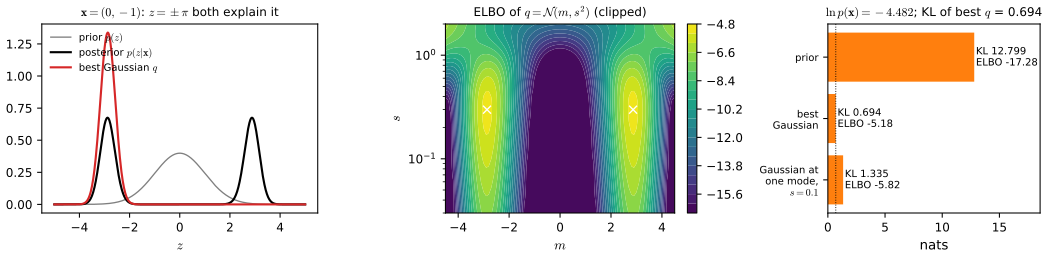
\({}=\E_{p(\bz\given\bx,\bw)}\big[\nabla_\bw\ln p(\bx,\bz\given\bw)\big]\) \({}=\nabla_\bw\L(q,\bw)\) at \(q=p(\bz\given\bx,\bw)\): the bound touches the log likelihood with the same slope. - If the posterior is an equal mixture \(\frac12(p_1+p_2)\) of two densities with disjoint supports, then for any \(q\) supported inside the support of \(p_1\), \(\KL(q\Vert p(\bz\given\bx))\)
\({}=\ln2+\KL(q\Vert p_1)\ge\ln2\). A single Gaussian sitting on one well-separated mode therefore pays at least \(\ln2\) nats.
Filling the gap 16.7: the decomposition, its conditions, the slope of the bound and the \(\ln2\) gap pp. 516–517; Exercises 16.18, 16.19
Derivation
(1) Use the product rule \(p(\bx,\bz\given\bw)\)
(2) With \(q(\bZ)=\prod_nq(\bz_n)\) and \(p(\bX,\bZ\given\bw)\)
(3) The E step sets \(q=p(\bz\given\bx,\bw^{\rm old})\), so \(\L(q,\bw^{\rm old})\)
(4) \(\nabla_\bw\ln p(\bx\given\bw)\)
(5) On the support of \(p_1\) the posterior equals \(\frac12p_1\), so \(\KL(q\Vert\frac12p_1)\)
16.3.1 Expectation maximization
See also the companion course, Section 12.2.2, Filling the gap 12.4 and Filling the gap 12.5 (missing values).
pp. 518–519 For probabilistic PCA EM may seem pointless, since the maximum likelihood solution is known in closed form. But in high dimensions EM can be cheaper, it extends to factor analysis (no closed form) and it handles missing data. The complete-data log likelihood is
\[ \ln p(\bX,\bZ\given\bmu,\bW,\sigma^2)=\sum_{n=1}^N\big\{\ln p(\bx_n\given\bz_n)+\ln p(\bz_n)\big\}, \tag{16.64} \]where row \(n\) of \(\bZ\) is \(\bz_n\). Setting \(\bmu=\bxbar\) and taking the expectation over the posterior,
\[ \E[\ln p(\bX,\bZ\given\bmu,\bW,\sigma^2)]=-\sum_{n=1}^N\Big\{\frac D2\ln(2\pi\sigma^2)+\frac12\Tr\big(\E[\bz_n\bz_n^\T]\big)+\frac1{2\sigma^2}\Vert\bx_n-\bmu\Vert^2-\frac1{\sigma^2}\E[\bz_n]^\T\bW^\T(\bx_n-\bmu)+\frac1{2\sigma^2}\Tr\big(\E[\bz_n\bz_n^\T]\bW^\T\bW\big)+\frac M2\ln(2\pi)\Big\}. \tag{16.65} \]It depends on the posterior only through its first two moments. The E step computes, with the old parameters,
\[ \E[\bz_n]=\bM^{-1}\bW^\T(\bx_n-\bxbar), \tag{16.66} \] \[ \E[\bz_n\bz_n^\T]=\sigma^2\bM^{-1}+\E[\bz_n]\E[\bz_n]^\T , \tag{16.67} \]and the M step sets
\[ \bW_{\rm new}=\Big[\sum_{n=1}^N(\bx_n-\bxbar)\E[\bz_n]^\T\Big]\Big[\sum_{n=1}^N\E[\bz_n\bz_n^\T]\Big]^{-1}, \tag{16.68} \] \[ \sigma^2_{\rm new}=\frac1{ND}\sum_{n=1}^N\Big\{\Vert\bx_n-\bxbar\Vert^2-2\E[\bz_n]^\T\bW_{\rm new}^\T(\bx_n-\bxbar)+\Tr\big(\E[\bz_n\bz_n^\T]\bW_{\rm new}^\T\bW_{\rm new}\big)\Big\}. \tag{16.69} \]Algorithm 16.3 (EM for probabilistic PCA) pp. 518–519, (16.66)–(16.69)
- Centre the data; initialise \(\bW\) (e.g. random) and \(\sigma^2>0\).
- E step: \(\bM=\bW^\T\bW+\sigma^2\bI\); for all \(n\), \(\E[\bz_n]\) and \(\E[\bz_n\bz_n^\T]\) by (16.66)–(16.67).
- M step: \(\bW\) by (16.68), then \(\sigma^2\) by (16.69) with the new \(\bW\).
- Repeat until the log likelihood (16.45) (computed with (16.41) and \(|\bC|=\sigma^{2(D-M)}|\bM|\)) stops increasing.
Filling the gap 16.8: the expected complete-data log likelihood, the M step, and the cost pp. 518–519, (16.65)–(16.69); Exercise 16.21
Derivation
(16.65). \(\ln p(\bx\given\bz)\)
(16.68). Using \(\partial\Tr(\mathbf B\bW^\T\bW)/\partial\bW\)
(16.69). With \(\bW=\bW_{\rm new}\) fixed, (16.65) is \(-\frac{ND}2\ln\sigma^2\)
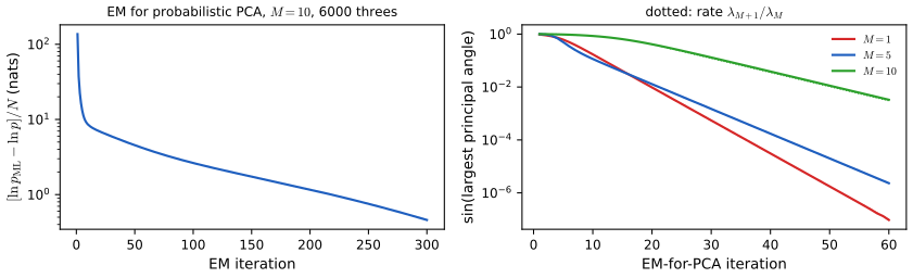
Cost. The E step needs \(\bW^\T(\bx_n-\bxbar)\) for all \(n\): \(O(NDM)\), plus \(O(DM^2+M^3)\) for \(\bM\) and its inverse. The M step needs \(\sum_n(\bx_n-\bxbar)\E[\bz_n]^\T\) (\(O(NDM)\)) and an \(M\times M\) inverse. Forming \(\bS\) would cost \(O(ND^2)\) and diagonalising it \(O(D^3)\); the snapshot method of Section 16.1.5 costs \(O(N^3)\). For large \(N\) and \(D\) with \(M\ll D\), EM's \(O(NDM)\) per iteration wins, and the sums can be accumulated one data point at a time (an online version that never stores the data set). The price is the number of iterations: convergence is linear, slow when the leading eigenvalues are close. On the 6000 threes with \(M=10\) (Figure 16.S4(a)), EM from a random start is still 0.46 nats per image below the maximum after 300 iterations. ∎
Result 16.13 (EM for probabilistic PCA with missing values) p. 519; Exercise 16.22
Let \(o_n\) be the observed coordinates of \(\bx_n\) and \(m_n\) the missing ones, assumed missing at random. With \(\bW_o\) the rows of \(\bW\) in \(o_n\), the E step uses \(\bM_n=\bW_o^\T\bW_o+\sigma^2\bI\), \(\E[\bz_n]\)
Proof
The latent variables are \(\bz_n\) and \(\bx_{n,m}\). Their joint posterior factorises as \(p(\bz_n\given\bx_{n,o})p(\bx_{n,m}\given\bz_n)\), because given \(\bz_n\) the coordinates of \(\bx_n\) are independent: the first factor is (16.43) with the observed rows, the second is \(\N(\bW_m\bz_n+\bmu_m,\sigma^2\bI)\). The complete-data log likelihood is \(\sum_n\sum_i\{-\frac12\ln2\pi\sigma^2-\frac1{2\sigma^2}(x_{ni}-\boldsymbol\theta_i^\T\widetilde\bz_n)^2\}\)
On "missing at random". The book defines it as missingness that depends neither on observed nor on unobserved values. That is missing completely at random; missing at random (Rubin, 1976) allows dependence on the observed values, and the likelihood-based EM above remains valid under that weaker condition, because the factor describing the missingness then does not involve the model parameters. ∎
16.3.2 EM for PCA
See also the companion course, Result 12.12 (EM for PCA is subspace iteration) and the EM view of its PCA demo.
pp. 519–520 In the limit \(\sigma^2\to0\) (standard PCA) EM still makes sense (Roweis, 1998). Only \(\E[\bz_n]\) is needed and \(\bM=\bW^\T\bW\). Let \(\bXt\) be the \(N\times D\) matrix with rows \((\bx_n-\bxbar)^\T\) and \(\bOm\) the \(M\times N\) matrix with columns \(\E[\bz_n]\). The E step (16.66) becomes
\[ \bOm=(\bW_{\rm old}^\T\bW_{\rm old})^{-1}\bW_{\rm old}^\T\bXt^\T \tag{16.70} \]and the M step (16.68)
\[ \bW_{\rm new}=\bXt^\T\bOm^\T(\bOm\bOm^\T)^{-1}. \tag{16.71} \]The E step projects the points orthogonally onto the current subspace; the M step moves the subspace to minimise the squared reconstruction error with the projections held fixed (Exercise 16.23). Picture a rod (the subspace) attached to each point by a spring: the E step lets the attachment points slide along the fixed rod to their lowest-energy positions (the orthogonal projections), and the M step releases the rod with the attachments fixed (Figure 16.10).
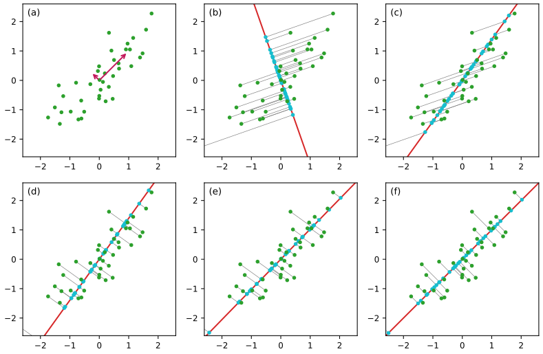
Result 16.14 (EM for PCA is subspace iteration) pp. 519–520, (16.70)–(16.71); Exercise 16.23
- (16.70) minimises \(J\)
\({}=\sum_n\Vert\bx_n-\bxbar-\bW\bz_n\Vert^2\) (16.90) over the \(\bz_n\) for fixed \(\bW\), and (16.71) minimises it over \(\bW\) for fixed \(\bz_n\). - \(\bW_{\rm new}\)
\({}=\bS\bW_{\rm old}(\bW_{\rm old}^\T\bS\bW_{\rm old})^{-1}\bW_{\rm old}^\T\bW_{\rm old}\), so \(\span\bW_{\rm new}\) \({}=\span(\bS\bW_{\rm old})\). - Hence, if \(\lambda_M>\lambda_{M+1}\) and the starting subspace is not orthogonal to any leading eigenvector, \(\span\bW\) converges to the principal subspace, with the sine of the largest principal angle shrinking by the factor \(\lambda_{M+1}/\lambda_M\) per iteration.
Filling the gap 16.9: alternating least squares, power iteration, and the rate p. 520, "a simple interpretation"; Exercise 16.23
Derivation
(1) For fixed \(\bW\), \(J\) is a sum of separate least-squares problems in \(\bz_n\), solved by \(\bz_n\)
(2) With \(\mathbf G=(\bW^\T\bW)^{-1}\): \(\bOm\bOm^\T\)
(3) So after \(k\) iterations \(\span\bW_k=\span(\bS^k\bW_0)\): this is orthogonal (subspace) iteration, the block power method. Writing \(\bW_0\) in the eigenbasis, the components along \(\bu_{M+1},\dots\) shrink relative to those along \(\bu_1,\dots,\bu_M\) by at least \((\lambda_{M+1}/\lambda_M)^k\) (Golub and Van Loan, 1996, Section 7.3). The measured rate is 0.8476 against \(\lambda_3/\lambda_2=0.8476\) on data with population eigenvalues 5, 4, 3.4, ...; Figure 16.S4(b) shows the same on the threes. Every fixed point spans an invariant subspace of \(\bS\), but only the principal one is stable. ∎
16.3.3 EM for factor analysis
See also the companion course, Filling the gap 12.7 and Algorithm 12.5.
pp. 520–521 For factor analysis \(\bmu=\bxbar\) again (Exercise 16.26), but \(\bW\) and \(\bPsi\) have no closed form; EM (Rubin and Thayer, 1982) has the E step
\[ \E[\bz_n]=\bG\bW^\T\bPsi^{-1}(\bx_n-\bxbar), \tag{16.72} \] \[ \E[\bz_n\bz_n^\T]=\bG+\E[\bz_n]\E[\bz_n]^\T , \tag{16.73} \] \[ \bG=(\bI+\bW^\T\bPsi^{-1}\bW)^{-1}, \tag{16.74} \]which inverts only \(M\times M\) matrices (and the diagonal \(\bPsi\), in \(O(D)\)), and the M step
\[ \bW_{\rm new}=\Big[\sum_{n=1}^N(\bx_n-\bxbar)\E[\bz_n]^\T\Big]\Big[\sum_{n=1}^N\E[\bz_n\bz_n^\T]\Big]^{-1}, \tag{16.75} \] \[ \bPsi_{\rm new}=\diag\Big\{\bS-\bW_{\rm new}\frac1N\sum_{n=1}^N\E[\bz_n](\bx_n-\bxbar)^\T\Big\}, \tag{16.76} \]where \(\diag\) sets the off-diagonal elements to zero.
Algorithm 16.4 (EM for factor analysis; Rubin and Thayer, 1982) pp. 520–521, (16.72)–(16.76)
- Centre the data, compute \(\bS\); initialise \(\bW\) and \(\bPsi\) (e.g. \(\bPsi=\diag\bS\)).
- E step: \(\bG\) by (16.74), then (16.72)–(16.73) for all \(n\).
- M step: \(\bW\) by (16.75), \(\bPsi\) by (16.76). Repeat until the log likelihood stops increasing.
Filling the gap 16.10: the E and M steps of factor analysis pp. 520–521; Exercises 16.24, 16.25
Derivation
E step. As a function of \(\bz\), \(\ln p(\bz)+\ln p(\bx\given\bz)\)
Expected complete-data log likelihood.
\[ \sum_n\Big\{-\frac12\ln|2\pi\bPsi|-\frac12\Tr\Big[\bPsi^{-1}\big((\bx_n-\bxbar)(\bx_n-\bxbar)^\T-2\bW\E[\bz_n](\bx_n-\bxbar)^\T+\bW\E[\bz_n\bz_n^\T]\bW^\T\big)\Big]\Big\}+(\text{terms without }\bW,\bPsi). \]
\(\bW\): the gradient \(\bPsi^{-1}\sum_n[(\bx_n\)
16.4 Nonlinear Latent Variable Models
See also the companion course, Section 12.4 (nonlinear latent variable models) and Advanced topics, lecture 1 (variational autoencoders); Section 2.4 of these notes (transformation of densities).
p. 522 Replace the linear map by a deep network. Start from a simple latent distribution
\[ p_{\bz}(\bz)=\N(\bz\given\bzero,\bI) \tag{16.77} \]and set \(\bx=\bg(\bz,\bw)\), a network with weights and biases \(\bw\). Sampling is easy and non-iterative: draw \(\bz\), apply the network. To fit \(\bw\) by maximum likelihood we need \(p(\bx\given\bw)\). If \(\bg\) is invertible, the change of variables gives
\[ p_{\bx}(\bx)=p_{\bz}(\bz(\bx))\,|\det\bJ(\bx)| , \tag{16.78} \] \[ J_{ij}(\bx)=\frac{\partial z_i}{\partial x_j}, \tag{16.79} \]which requires \(\bz=\bg^{-1}(\bx,\bw)\). For most networks the inverse does not exist (many-to-one maps), and if \(\dim\bz\ne\dim\bx\) the map cannot be invertible. Restricting to invertible networks of equal dimension leads to normalizing flows (Chapter 18).
Filling the gap 16.11: what goes wrong with (16.78) when \(\bg\) is not invertible or \(M<D\) pp. 522–523
The book says the formula "does not give a well-defined density". The two cases fail in different ways, and only one of them actually lacks a density.
Derivation
Invertible case. If \(\bg\) is a \(C^1\) bijection with non-singular Jacobian, then for any set \(B\), \(P(\bx\in B)=P(\bz\in\bg^{-1}(B))\)
Many-to-one, \(M=D\). If \(\bg\) is \(C^1\) and each \(\bx\) has finitely many preimages \(\bz^{(k)}\), all with non-singular Jacobian, splitting the latent space into pieces on which \(\bg\) is invertible gives \(p_\bx(\bx)\)
\(M<D\). The image \(\bg(\R^M)\) of a \(C^1\) (indeed locally Lipschitz) map is a set of Lebesgue measure zero in \(\R^D\). The distribution of \(\bx\) puts probability 1 on it, so it has no density with respect to Lebesgue measure: \(p(\bx)\) is "zero off the manifold and infinite on it". Any data point not exactly on the manifold has likelihood zero, and small changes of \(\bw\) do not change that, so the gradient is zero. Adding noise (16.80) convolves the singular distribution with a Gaussian, producing the smooth, everywhere-positive density \(p(\bx)\)
16.4.1 Nonlinear manifolds
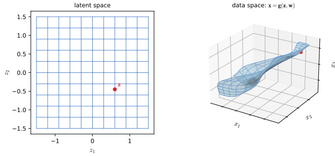
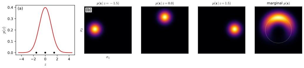
pp. 522–524 With \(M<D\) the distribution of \(\bg(\bz,\bw)\) is confined to an \(M\)-dimensional manifold (Figure 16.11). This encodes the inductive bias that data such as natural images do not fill their space (Section 6.1.4), even if the manifold's shape and dimension are unknown. To get a density on the whole space we add noise, as in regression:
\[ p(\bx\given\bz,\bw)=\N(\bx\given\bg(\bz,\bw),\sigma^2\bI), \tag{16.80} \]with a network with linear outputs, \(\bg\in\R^D\) (Figure 16.12, the two-node graph \(\bz\to\bx\), is not reproduced). Sampling takes three steps: draw \(\bz\) (Section 14.1.2), compute \(\bg(\bz,\bw)\), add Gaussian noise. The marginal is
\[ p(\bx)=\int p(\bz)p(\bx\given\bz)\,\d\bz . \tag{16.81} \]Definition 16.6 (nonlinear latent variable model) pp. 522–524, (16.77), (16.80), (16.81)
\(\bz\sim\N(\bzero,\bI_M)\), \(\bx\given\bz\sim\N(\bg(\bz,\bw),\sigma^2\bI_D)\) with \(\bg\) a neural network with linear outputs. Probabilistic PCA is the case \(\bg(\bz,\bw)=\bW\bz+\bmu\).
16.4.2 Likelihood function
pp. 524–525 The likelihood
\[ p(\bx\given\bw)=\int p(\bx\given\bz,\bw)p(\bz)\,\d\bz=\int\N(\bx\given\bg(\bz,\bw),\sigma^2\bI)\N(\bz\given\bzero,\bI)\,\d\bz \tag{16.82} \]is intractable: both factors are Gaussian, but \(\bg\) is nonlinear. One could sample the prior,
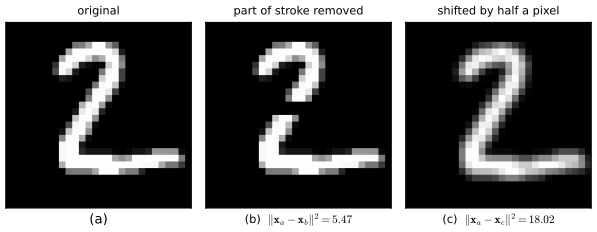
\[ p(\bx\given\bw)\simeq\frac1K\sum_{i=1}^Kp(\bx\given\bz_i,\bw),\qquad\bz_i\sim p(\bz), \tag{16.83} \]which treats the model as a mixture of \(K\) Gaussians with weights \(1/K\) and is exact as \(K\to\infty\). But the \(K\) needed is far too large. The book's example (Figure 16.14, from Doersch, 2016) shows why: under a Gaussian \(p(\bx\given\bz)\) the likelihood falls off with squared distance, and squared distance ranks a visibly damaged digit closer to the original than a perfect copy shifted by half a pixel. A \(\sigma\) small enough to reject the damaged digit rejects the shifted one too, so only latent samples that reproduce \(\bx\) almost pixel for pixel contribute, and they are rare.
Result 16.15 (the Monte Carlo likelihood (16.83): unbiased, biased in log, and exponentially costly in \(M\)) pp. 524–525
Let \(\widehat p_K\)
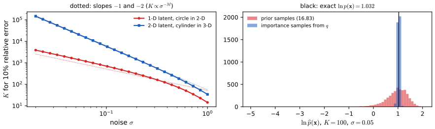
- \(\E[\widehat p_K]=p(\bx)\) and \(\var[\widehat p_K]/p(\bx)^2=\rho/K\); so \(K\approx\rho/\varepsilon^2\) samples give relative error \(\varepsilon\).
- \(\E[\ln\widehat p_K]\le\ln p(\bx)\) (Jensen), and \(\E[\ln\widehat p_K]\)
\({}=\ln p(\bx)-\rho/(2K)+o(1/K)\). - For Gaussian noise (16.80), if \(\bx=\bg(\bz^\star)\) lies on the manifold at a unique \(\bz^\star\) with \(\bJ=\partial\bg/\partial\bz\) of full rank \(M\), then as \(\sigma\to0\) \[ 1+\rho\approx\frac{|\bJ^\T\bJ|^{1/2}}{p(\bz^\star)\,(2\sqrt\pi\,\sigma)^M}, \] so the samples needed grow like \(\sigma^{-M}\): exponentially in the latent dimension.
- Sampling \(\bz_i\) from a \(q(\bz)\) close to the posterior and averaging \(p(\bx,\bz_i)/q(\bz_i)\) is unbiased with zero variance when \(q=p(\bz\given\bx)\); and \(\E\ln\) of this importance-weighted estimate lies between the ELBO \(\L(q)\) and \(\ln p(\bx)\) (Burda, Grosse and Salakhutdinov, 2016).
Filling the gap 16.12: how many samples does (16.83) need? p. 525, "the value of \(K\) needed for effective training will typically be far too high"
Derivation
(1)–(2). The terms \(p(\bx\given\bz_i)\) are i.i.d. with mean \(\int p(\bx\given\bz)p(\bz)\d\bz=p(\bx)\), so the average is unbiased with variance \(\var[p(\bx\given\bz)]/K\). Jensen's inequality for the concave logarithm gives \(\E\ln\widehat p_K\le\ln\E\widehat p_K\). For the expansion write \(\widehat p_K=p(1+\delta)\) with \(\E\delta=0\), \(\E\delta^2=\rho/K\): \(\ln(1+\delta)\)
(3). For a Gaussian, \(\N(\bx\given\bg,\sigma^2\bI)^2\)
(4). \(p(\bx)\)
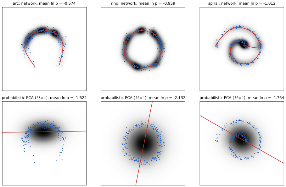
Training anyway, in low dimension. With \(M=1\) the integral (16.82) can be done by quadrature, and a small network can be trained by maximum likelihood directly. Figure 16.S7 does this on three two-dimensional data sets and compares with probabilistic PCA, the linear special case; the demo trains the same network live and contrasts the grid with Monte Carlo samples.
16.4.3 Discrete data
p. 526 For independent binary variables the network outputs Bernoulli probabilities,
\[ p(\bx\given\bz,\bw)=\prod_{i=1}^Dg_i(\bz,\bw)^{x_i}\big(1-g_i(\bz,\bw)\big)^{1-x_i}, \tag{16.84} \]with \(g_i=\sigma(a_i(\bz,\bw))\) the logistic sigmoid of the pre-activation \(a_i\). For one-hot categorical variables,
\[ p(\bx\given\bz,\bw)=\prod_{i=1}^Dg_i(\bz,\bw)^{x_i}, \tag{16.85} \] \[ g_i(\bz,\bw)=\frac{\exp(a_i(\bz,\bw))}{\sum_j\exp(a_j(\bz,\bw))}, \tag{16.86} \]and mixed data use products of such factors. Continuous quantities are usually stored discretised, e.g. 8-bit intensities \(\{0,\dots,255\}\); a flexible density model can then collapse onto those values and its likelihood can grow without limit. Dequantisation adds noise, typically uniform over the interval between successive values, replacing each training value by a random point of its interval (Figure 16.15).
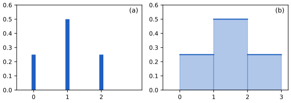
Result 16.16 (why dequantisation works) p. 526, Figure 16.15
- Without it, a continuous model can have unbounded likelihood on discrete data: Gaussians of width \(s\) centred on the data values give \(\ln p\to+\infty\) as \(s\to0\).
- For any density \(p\) on \(\R^D\) define the discrete model \(P(\bx)=\int_{[0,1)^D}p(\bx+\bu)\,\d\bu\) on integer vectors. Then \(\E_{\bu\sim\Unif[0,1)^D}[\ln p(\bx+\bu)]\)
\({}\le\ln P(\bx)\le0\). So the dequantised log likelihood is a lower bound on the log probability of a proper discrete model, bounded above by 0; equality holds when \(p\) is constant on each cell.
Filling the gap 16.13: dequantisation as a lower bound p. 526, "this makes it less likely that the model will discover a pathological solution"
Derivation
(1) For data \(x_n\in\{0,1,2,\dots\}\) and the mixture \(p_s(x)=\frac1K\sum_{k}\N(x\given k,s^2)\) over the \(K\) distinct values, each data point contributes at least \(\ln\{\frac1K\N(x_n\given x_n,s^2)\}\)
(2) \(\bu\mapsto p(\bx+\bu)\) is a density times 1 on the unit cube, so by Jensen's inequality for the concave logarithm and a uniform \(\bu\), \(\E_\bu[\ln p(\bx+\bu)]\)
16.4.4 Four approaches to generative modelling
See also the companion course, Advanced topics: variational autoencoders (lecture 1), normalizing flows (lecture 2) and diffusion models (lecture 4).
p. 527 Nonlinear latent variable models can approximate essentially any distribution and sample in one pass, but the likelihood is the obstacle. The rest of the book follows four ways around it:
| Approach | What changes | Likelihood | Sampling | Book |
|---|---|---|---|---|
| Generative adversarial networks | \(M<D\) allowed, no likelihood; a second network (discriminator) provides the training signal | none | one pass | Chapter 17 |
| Variational autoencoders | a second network approximates \(p(\bz\given\bx)\); train on the ELBO (16.58) | lower bound | one pass | Chapter 19 |
| Normalizing flows | \(M=D\) and \(\bg\) invertible; use (16.78) | exact | one pass | Chapter 18 |
| Diffusion models | a network learns to undo many small noising steps | bound | many passes | Chapter 20 |
GAN training can be brittle but gives high-quality samples; VAE training is more robust but the best sample quality is harder to reach; flows are restricted in form; diffusion models give state-of-the-art results at the price of many network evaluations per sample.
Summary: errors and imprecisions found in the chapter (first printing)
- p. 495: MNIST digits are \(28\times28\) images, not "\(64\times64\)" (the book's own Figure 16.3 caption says \(28\times28\)).
- (16.57) and (16.60): \(\L(\bw)\) should be \(\L(q,\bw)\), as in (16.58); the bound depends on \(q\).
- p. 510: with \(\bR=\bI\) the columns of \(\bW_{\rm ML}\) are the eigenvectors scaled by \((\lambda_i-\sigma^2)^{1/2}\), not by \(\lambda_i-\sigma^2\) (from (16.46); checked: \(\bu_i^\T\bC\bu_i=\lambda_i\) only with the square root).
- p. 519: the definition given for "missing at random" (missingness independent of observed and unobserved values) is that of missing completely at random; EM remains valid under the weaker missing-at-random condition (Rubin, 1976).
- pp. 498, 506 (cross-references): the EM algorithm for probabilistic PCA is in Section 16.3.1; Section 16.3.2 is its zero-noise limit.
- Exercise 16.13, (16.88): the reconstruction needs \(+\bxbar\) unless \(\bx\) is centred.
- Exercise 16.17: "\(p(\bz)=\N(\bx\given\bzero,\bI)\)" should read \(\N(\bz\given\bzero,\bI)\).
- p. 514 (imprecision): a component-wise rescaling of the data is absorbed by \(\bPsi\) and by the rows of \(\bW\) (Result 16.9).
- p. 522 (imprecision): for a many-to-one \(\bg\) with \(M=D\) a density still exists (a sum over preimages); the difficulty is evaluating it. Only for \(M<D\) is there no density (Filling the gap 16.11).
- Section 16.2.6 (terminology): the model is the linear dynamical system; the Kalman filter is the inference algorithm for it.
Exercises
All 26 exercises of Chapter 16 (Bishop and Bishop, 2024, pp. 527–531), restated in my own words, with complete solutions (hidden). Stars give the book's difficulty. The official solutions manual stops at Chapter 10, so these solutions are my own; most exercises correspond to exercises of Bishop (2006), Chapter 12, and the companion course's solution is linked.
Exercise 16.1 (★★). Show by induction on \(M\) that the \(M\)-dimensional projection maximising the projected variance is given by the eigenvectors of \(\bS\) with the \(M\) largest eigenvalues: given the result for \(M\), use Lagrange multipliers for normalisation and orthogonality to \(\bu_1,\dots,\bu_M\) to show that \(\bu_{M+1}\) is an eigenvector, then that its eigenvalue must be \(\lambda_{M+1}\).
Solution
The step is written out in Filling the gap 16.1: stationarity gives \(2\bS\bu-2\lambda\bu+\sum_j\eta_j\bu_j\)
\({}=\bzero\); multiplying by \(\bu_k^\T\) and using \(\bS\bu_k=\lambda_k\bu_k\), \(\bu_k^\T\bu=0\), gives \(\eta_k=0\), so \(\bS\bu=\lambda\bu\) with \(\bu\perp\bu_1,\dots,\bu_M\). The variance \(\bu^\T\bS\bu=\lambda\) is then maximised by the largest eigenvalue among the remaining eigenvectors, \(\lambda_{M+1}\). The base case is (16.5)–(16.6). That the greedy choice is also optimal among all \(M\)-dimensional subspaces is Result 16.1. (Companion Exercise 12.1.) Exercise 16.2 (★★). Minimise (16.15) under the orthonormality constraints using a symmetric matrix \(\bH\) of multipliers, (16.87); show that the solution satisfies \(\bS\widehat\bU=\widehat\bU\bH\), and that every solution gives the same \(J\) as one whose columns are eigenvectors.
Solution
See Filling the gap 16.2: only the symmetric part of \(\bH\) enters (16.87); the gradient \(2\bS\widehat\bU-2\widehat\bU\bH\) vanishes iff \(\bS\widehat\bU=\widehat\bU\bH\); then \(\bH=\widehat\bU^\T\bS\widehat\bU\), and with \(\bH=\bPsi\Lambda\bPsi^\T\) the columns of \(\widehat\bU\bPsi\) are orthonormal eigenvectors and \(J=\Tr\bH=\Tr\Lambda\). The minimum discards the \(D-M\) smallest eigenvalues. (Companion Exercise 12.2.)
Exercise 16.3 (★). Show that (16.30) has unit length when \(\bv_i\) does.
Solution
\(\Vert\bX^\T\bv_i\Vert^2\)
\({}=\bv_i^\T\bX\bX^\T\bv_i\) \({}=\bv_i^\T(N\lambda_i\bv_i)=N\lambda_i\) by (16.28), so \(\Vert\bu_i\Vert^2\) \({}=N\lambda_i/(N\lambda_i)=1\). (Needs \(\lambda_i>0\). Companion Exercise 12.3.) Exercise 16.4 (★). Replace the prior (16.31) by \(\N(\bz\given\mathbf m,\Sig)\). Show that, after redefining the parameters, the marginal of \(\bx\) is the same family as before.
Solution
Write \(\bz=\mathbf m+\Sig^{1/2}\bz'\) with \(\bz'\sim\N(\bzero,\bI)\). Then \(\bx\)
\({}=\bW\Sig^{1/2}\bz'+(\bmu+\bW\mathbf m)\) \({}+\beps\), a standard PPCA with \(\bW'=\bW\Sig^{1/2}\), \(\bmu'=\bmu+\bW\mathbf m\): marginal \(\N(\bmu+\bW\mathbf m,\bW\Sig\bW^\T\) \({}+\sigma^2\bI)\). Every pair \((\bW',\bmu')\) arises (take \(\bW=\bW'\Sig^{-1/2}\), \(\bmu=\bmu'-\bW\mathbf m\)), so the family of marginals is unchanged. (Result 16.5(4); companion Exercise 12.4.) Exercise 16.5 (★★). If \(\bx\sim\N(\bmu,\Sig)\) in \(\R^D\) and \(\by=\bA\bx+\mathbf b\) with \(\bA\) an \(M\times D\) matrix, show that \(\by\) is Gaussian, find its mean and covariance, and discuss \(M<D\), \(M=D\), \(M>D\).
Solution
The moment generating function is \(\E e^{\mathbf t^\T\by}\)
\({}=e^{\mathbf t^\T\mathbf b}\E e^{(\bA^\T\mathbf t)^\T\bx}\) \({}=\exp\{\mathbf t^\T(\bA\bmu+\mathbf b)+\frac12\mathbf t^\T\bA\Sig\bA^\T\mathbf t\}\), that of \(\N(\bA\bmu+\mathbf b,\bA\Sig\bA^\T)\). For \(M<D\) with \(\bA\) of full row rank, \(\bA\Sig\bA^\T\) is positive definite (\(\mathbf t^\T\bA\Sig\bA^\T\mathbf t\) \({}=(\bA^\T\mathbf t)^\T\Sig(\bA^\T\mathbf t)\) \({}>0\) for \(\mathbf t\ne\bzero\)) and \(\by\) has a density; marginalisation is the case of a selection matrix. For \(M=D\), \(\by\) has a density iff \(\bA\) is invertible (then also by the change of variables (16.78)). For \(M>D\), \(\operatorname{rank}\bA\Sig\bA^\T\le D\) \({}<M\): the Gaussian is degenerate, concentrated on the affine subspace \(\mathbf b+\operatorname{range}\bA\), and has no density on \(\R^M\), which is the singular case of Filling the gap 16.11. (Companion Exercise 12.5.) Exercise 16.6 (★★). Derive (16.35) from the general formulae (2.122)–(2.123) for the mean and covariance in terms of conditional moments.
Solution
\(\E[\bx]=\E_\bz[\E[\bx\given\bz]]\)
\({}=\E[\bW\bz+\bmu]=\bmu\) and \(\cov[\bx]\) \({}=\E_\bz[\cov[\bx\given\bz]]\) \({}+\cov_\bz[\E[\bx\given\bz]]\) \({}=\sigma^2\bI+\bW\cov[\bz]\bW^\T\) \({}=\bW\bW^\T+\sigma^2\bI\). Gaussianity: \(\bx\) is an affine function of the jointly Gaussian \((\bz,\beps)\) (Exercise 16.5). (Companion Exercise 12.7.) Exercise 16.7 (★). Draw the directed graph of probabilistic PCA with each component of \(\bx\) as its own node, and check that it has the independence structure of the naive Bayes model.
Solution
Nodes: \(\bz\) (or its components), and \(x_1,\dots,x_D\); edges \(\bz\to x_i\) for every \(i\), plus parameter nodes \(\bw_i\) (row \(i\) of \(\bW\)), \(\mu_i\) and \(\sigma^2\) pointing into \(x_i\); no edges among the \(x_i\). Every path between \(x_i\) and \(x_j\) passes through \(\bz\) tail-to-tail, so it is blocked when \(\bz\) is observed: \(x_i\perp x_j\given\bz\), as the factorisation \(p(\bx\given\bz)\)
\({}=\prod_i\N(x_i\given\bw_i^\T\bz\) \({}+\mu_i,\sigma^2)\) confirms. This is the naive Bayes structure (Section 11.2.3) with a continuous "class" \(\bz\). (Companion Exercise 12.6.) Exercise 16.8 (★★). Using (3.100), show that the posterior of probabilistic PCA is (16.43).
Solution
(3.100) states that for \(p(\bz)\)
\({}=\N(\bmu_z,\boldsymbol\Lambda^{-1})\) and \(p(\bx\given\bz)\) \({}=\N(\bA\bz+\mathbf b,\bL^{-1})\), \(p(\bz\given\bx)\) \({}=\N(\Sig\{\bA^\T\bL(\bx-\mathbf b)+\boldsymbol\Lambda\bmu_z\},\Sig)\), \(\Sig\) \({}=(\boldsymbol\Lambda+\bA^\T\bL\bA)^{-1}\). Substitute \(\bmu_z=\bzero\), \(\boldsymbol\Lambda=\bI\), \(\bA=\bW\), \(\mathbf b=\bmu\), \(\bL=\sigma^{-2}\bI\): \(\Sig=(\bI+\sigma^{-2}\bW^\T\bW)^{-1}\) \({}=\sigma^2\bM^{-1}\), mean \(\sigma^2\bM^{-1}\sigma^{-2}\bW^\T(\bx\) \({}-\bmu)\) \({}=\bM^{-1}\bW^\T(\bx-\bmu)\). (Companion Exercise 12.8.) Exercise 16.9 (★). Show that maximising (16.44) over \(\bmu\) gives \(\bmu_{\rm ML}=\bxbar\).
Solution
\(\partial/\partial\bmu\) of (16.44) is \(\sum_n\bC^{-1}(\bx_n-\bmu)\)
\({}=\bC^{-1}N(\bxbar-\bmu)\), zero iff \(\bmu=\bxbar\) since \(\bC\) is invertible. (Companion Exercise 12.9.) Exercise 16.10 (★★). Using second derivatives, show that \(\bmu=\bxbar\) is the unique maximum.
Solution
The Hessian of (16.44) with respect to \(\bmu\) is \(-N\bC^{-1}\), negative definite and independent of \(\bmu\). The log likelihood is therefore a strictly concave quadratic in \(\bmu\), whose only stationary point \(\bxbar\) is the global maximum. (Checked numerically; companion Exercise 12.10.)
Exercise 16.11 (★★). Show that as \(\sigma^2\to0\) the posterior mean becomes an orthogonal projection onto the principal subspace, as in PCA.
Solution
As \(\sigma^2\to0\), \(\bM\to\bW^\T\bW\) and \(\E[\bz\given\bx]\)
\({}\to(\bW^\T\bW)^{-1}\bW^\T(\bx-\bxbar)\) (16.51), the least-squares coordinates of \(\bx-\bxbar\) in the basis given by the columns of \(\bW\); mapped back, \(\bW(\bW^\T\bW)^{-1}\bW^\T(\bx-\bxbar)\) is the orthogonal projector onto \(\span\bW\), the principal subspace, applied to \(\bx-\bxbar\). (With \(\bW_{\rm ML}\) also depending on \(\sigma^2\), its column space stays \(\span\bU_M\), so the limit is the same; Result 16.7; companion Exercise 12.11.) Exercise 16.12 (★★). For \(\sigma^2>0\), show that the posterior mean is shrunk towards the origin relative to the orthogonal projection.
Solution
By Result 16.7, in the eigenbasis (with \(\bR=\bI\)) each coordinate of the posterior mean is the coordinate of the orthogonal projection (16.51) times \((\lambda_j-\sigma^2)/\lambda_j\in[0,1)\). For general \(\bR\) both vectors are rotated by \(\bR^\T\), which preserves lengths, so \(\Vert\E[\bz\given\bx]\Vert\)
\({}<\Vert(\bW^\T\bW)^{-1}\bW^\T(\bx\) \({}-\bxbar)\Vert\) whenever the projection is non-zero. (Checked numerically; companion Exercise 12.12.) Exercise 16.13 (★★). Show that the least-squares optimal reconstruction from the posterior mean is (16.88).
Solution
Look for \(\bxt=\bW\mathbf c+\bxbar\) minimising \(\Vert\bx-\bxt\Vert^2\): \(\mathbf c\)
\({}=(\bW^\T\bW)^{-1}\bW^\T(\bx-\bxbar)\). By (16.49), \(\bW^\T(\bx-\bxbar)=\bM\E[\bz\given\bx]\), so \(\bxt\) \({}=\bW(\bW^\T\bW)^{-1}\bM\E[\bz\given\bx]\) \({}+\bxbar\), the orthogonal projection onto the principal subspace, identical to the PCA reconstruction (16.20) (Result 16.7). The book's (16.88) omits \(\bxbar\). (Companion Exercise 12.13.) Exercise 16.14 (★). Verify that (16.52) gives the count of a general covariance for \(M=D-1\) and of an isotropic covariance for \(M=0\).
Solution
\(M=D-1\): \(D(D-1)+1-\frac{(D-1)(D-2)}2\)
\({}=\frac{2D^2-2D+2-D^2+3D-2}2\) \({}=\frac{D(D+1)}2\). \(M=0\): \(0+1-0=1\). (Confirmed by Jacobian ranks in Result 16.8; companion Exercise 12.14.) Exercise 16.15 (★). Find the number of independent parameters of factor analysis.
Solution
\(\bW\) has \(DM\) entries, \(\bPsi\) has \(D\), and rotations remove \(M(M-1)/2\): \(DM+D-M(M-1)/2\) for the covariance, plus \(D\) for \(\bmu\). The count is meaningful only while it does not exceed \(D(D+1)/2\) (otherwise the model is not identifiable). (Result 16.8: rank 20 for \(D=7\), \(M=2\); companion Exercise 12.18.)
Exercise 16.16 (★★). Show that factor analysis is invariant under rotations of the latent coordinates.
Solution
Replace \(\bz\) by \(\bz'=\bR^\T\bz\) with \(\bR\) orthogonal; \(\bz'\sim\N(\bzero,\bR^\T\bR)\)
\({}=\N(\bzero,\bI)\) and \(\bW\bz=\bW\bR\bz'\), so the model with \(\bW\bR\) generates the same \(\bx\). Equivalently, \(\bW\bR(\bW\bR)^\T+\bPsi=\bW\bW^\T+\bPsi\): the marginal and the likelihood are unchanged. (Checked numerically; companion Exercise 12.19.) Exercise 16.17 (★★). For \(p(\bz)=\N(\bz\given\bzero,\bI)\) and \(p(\bx\given\bz)=\N(\bW\bz+\bmu,\bPhi)\) with \(\bPhi\) symmetric positive definite, show that if \((\bmu,\bW,\bPhi)_{\rm ML}\) fits \(\{\bx_n\}\) then \((\bA\bmu,\bA\bW,\bA\bPhi\bA^\T)\) fits \(\{\bA\bx_n\}\); and that the model's form is kept (i) for diagonal \(\bA\) and diagonal \(\bPhi\) (factor analysis), (ii) for orthogonal \(\bA\) and \(\bPhi=\sigma^2\bI\) (PPCA).
Solution
See Result 16.9: the transformed log likelihood equals the original minus \(N\ln|\det\bA|\), and the parameter map is a bijection when it preserves the constraint on \(\bPhi\); (i) \(\bA\bPsi\bA^\T=\diag(a_i^2\psi_i)\) is diagonal; (ii) \(\bA\sigma^2\bI\bA^\T=\sigma^2\bI\). Factor analysis is therefore covariant under rescaling of each variable, PPCA under rotations of data space (as is PCA). (Note the typo \(\N(\bx\given\bzero,\bI)\) in the book's statement. Companion Exercise 12.25.)
Exercise 16.18 (★). Verify (16.57)–(16.59) using the product rule (16.89).
Solution
Filling the gap 16.7, part (1): insert \(p(\bx,\bz\given\bw)\)
\({}=p(\bz\given\bx,\bw)p(\bx\given\bw)\) in (16.58) and use \(\int q=1\). (Companion Exercise 9.24, the discrete version.) Exercise 16.19 (★). Show that for i.i.d. data the ELBO has the form (16.63).
Solution
Filling the gap 16.7, part (2): with \(q(\bZ)=\prod_nq(\bz_n)\), the log ratio is a sum over \(n\) and each term integrates against its own factor.
Exercise 16.20 (★★). Draw the graphical model of a mixture of probabilistic PCA models, each with its own \(\bW\), \(\bmu\), \(\sigma^2\); then the graph in which these are shared by all components.
Solution
Inside a plate over \(n=1,\dots,N\): a discrete node \(s_n\) (the component, with parent \(\boldsymbol\pi\) outside the plate), a continuous node \(\bz_n\) (no parents, prior \(\N(\bzero,\bI)\)), and \(\bx_n\) with parents \(s_n\) and \(\bz_n\). Outside the plate, a plate over \(k=1,\dots,K\) holds \(\bW_k,\bmu_k,\sigma_k^2\), all pointing into \(\bx_n\); then \(p(\bx_n\given s_n=k,\bz_n)\)
\({}=\N(\bW_k\bz_n+\bmu_k,\sigma_k^2\bI)\). If the parameters are shared, the \(K\)-plate disappears and \(\bW,\bmu,\sigma^2\) point into \(\bx_n\) directly; the edge \(s_n\to\bx_n\) then carries no information (\(p(\bx_n\given s_n,\bz_n)\) does not depend on \(s_n\)) and can be deleted: the mixture collapses to a single PPCA model with \(s_n\) disconnected. Sharing only \(\bW\) and \(\sigma^2\) but not \(\bmu_k\) would give a genuine mixture of shifted copies. (Companion Exercise 12.23.) Exercise 16.21 (★★). Derive the M step (16.68)–(16.69) by maximising (16.65).
Solution
Filling the gap 16.8. (Companion Exercise 12.15.)
Exercise 16.22 (★★★). Derive EM for probabilistic PCA when values are missing at random, treating both the \(\bz_n\) and the missing entries as latent; show that it reduces to Section 16.3.1 when nothing is missing.
Solution
Result 16.13 and its proof: the posterior factorises as \(p(\bz_n\given\bx_{n,o})p(\bx_{n,m}\given\bz_n)\); the E step computes the moments of \(\bz_n\) from the observed rows and fills in \(\E[x_{ni}\widetilde\bz_n]\) and \(\E[x_{ni}^2]\) for missing entries; the M step is a least-squares problem per row \((\bw_i,\mu_i)\) and an average for \(\sigma^2\). Without missing values \(\sum_n\E[\bz_n]=\bzero\) when \(\bmu=\bxbar\), so \(\bmu\) stays at \(\bxbar\) and the updates are (16.66)–(16.69) (checked to \(10^{-10}\)). (Companion Exercise 12.16.)
Exercise 16.23 (★★). For \(J=\sum_n\Vert\bx_n-\bmu-\bW\bz_n\Vert^2\) (16.90), show that minimising over \(\bmu\) leads to the same problem with centred \(\bx_n-\bxbar\) and \(\bz_n-\bar\bz\); that minimising over the \(\bz_n\) is the E step (16.70); and over \(\bW\) the M step (16.71).
Solution
\(\partial J/\partial\bmu\)
\({}=-2\sum_n(\bx_n-\bmu-\bW\bz_n)=\bzero\) gives \(\bmu=\bxbar-\bW\bar\bz\); substituting, \(\bx_n-\bmu-\bW\bz_n\) \({}=(\bx_n-\bxbar)-\bW(\bz_n-\bar\bz)\). The other two parts are Result 16.14(1) with its proof in Filling the gap 16.9. (Companion Exercise 12.17.) Exercise 16.24 (★★). Derive the E step (16.72)–(16.73) of factor analysis (using Exercise 16.26 to set \(\bmu=\bxbar\)).
Solution
Filling the gap 16.10, E step: complete the square in \(\bz\) to get precision \(\bI+\bW^\T\bPsi^{-1}\bW=\bG^{-1}\) and mean \(\bG\bW^\T\bPsi^{-1}(\bx-\bxbar)\); then \(\E[\bz\bz^\T]=\bG+\E[\bz]\E[\bz]^\T\). (Companion Exercise 12.21.)
Exercise 16.25 (★★). Write the expected complete-data log likelihood of factor analysis and derive the M step (16.75)–(16.76).
Solution
Filling the gap 16.10, M step: the expectation is displayed there; the \(\bW\)-gradient gives (16.75); the derivative in each \(\psi_i\), simplified with (16.75), gives (16.76). (Companion Exercise 12.22.)
Exercise 16.26 (★★). Show that the only stationary point of the factor analysis log likelihood with respect to \(\bmu\) is \(\bxbar\), and that it is a maximum.
Solution
The log likelihood is (16.44) with \(\bC=\bW\bW^\T+\bPsi\), positive definite. Its gradient in \(\bmu\) is \(N\bC^{-1}(\bxbar-\bmu)\), zero only at \(\bxbar\), and its Hessian \(-N\bC^{-1}\) is negative definite everywhere: a strictly concave quadratic with unique maximum \(\bxbar\). (Companion Exercise 12.20.)
Demonstrations
Three interactive pages, each linked above where its topic arises. They reproduce the Python code number for number (largest differences \(8\times10^{-16}\) relative for the eigen-digits, \(7\times10^{-15}\) for the ICA run, \(2\times10^{-14}\) for the trained network and the ELBO). The companion course already has demonstrations of two-dimensional PCA and whitening, EM for PCA, Bayesian PCA, kernel PCA, the Kalman filter and the EM bound (listed above), so the pages here concentrate on what this chapter adds.
- Eigen-digits: PCA compression of MNIST threes with the eigenvectors computed in Python; reconstruction, residual, coefficients, the error against \(M\) and the probabilistic PCA likelihood of other digits. Presets: 1 \(M=1\), 2 \(M=10\), 3 \(M=50\), 4 \(M=250\), 5 a 7 through the threes.
- Independent component analysis: mixing, whitening, the likelihood along rotations and natural-gradient unmixing with the sech or a light-tailed prior. Presets: 1 heavy-tailed sources, 2 Gaussian sources, 3 uniform sources, sech prior, 4 light-tailed prior, 5 sine and sawtooth.
- A nonlinear latent variable model in two dimensions: the circle model of Figure 16.13, the posterior and ELBO of any point, a network \(\bg(z,\bw)\) trained in the browser, and the Monte Carlo likelihood (16.83). Presets: 1 the book's model, 2 a two-mode posterior, 3 train on an arc, 4 a closed ring, 5 Monte Carlo with \(K=4\).
References
- Bishop, C. M. and Bishop, H. (2024). Deep Learning: Foundations and Concepts. Springer, Cham. Chapter 16, pp. 495–531. doi:10.1007/978-3-031-45468-4. Book website: www.bishopbook.com.
- Bishop, C. M. (2006). Pattern Recognition and Machine Learning. Springer. Chapters 12 and 13.
- Amari, S., Cichocki, A. and Yang, H. H. (1996). A new learning algorithm for blind signal separation. In Advances in Neural Information Processing Systems 8, 757–763.
- Anderson, T. W. (1963). Asymptotic theory for principal component analysis. Annals of Mathematical Statistics, 34(1), 122–148.
- Attias, H. (1999). Independent factor analysis. Neural Computation, 11(4), 803–851.
- Bell, A. J. and Sejnowski, T. J. (1995). An information-maximization approach to blind separation and blind deconvolution. Neural Computation, 7(6), 1129–1159.
- Burda, Y., Grosse, R. and Salakhutdinov, R. (2016). Importance weighted autoencoders. In International Conference on Learning Representations.
- Cardoso, J.-F. (1998). Blind signal separation: statistical principles. Proceedings of the IEEE, 86(10), 2009–2025.
- Comon, P. (1994). Independent component analysis, a new concept? Signal Processing, 36(3), 287–314.
- Doersch, C. (2016). Tutorial on variational autoencoders. arXiv:1606.05908.
- Golub, G. H. and Van Loan, C. F. (1996). Matrix Computations (3rd ed.). Johns Hopkins University Press.
- Hotelling, H. (1933). Analysis of a complex of statistical variables into principal components. Journal of Educational Psychology, 24, 417–441 and 498–520.
- Hotelling, H. (1936). Relations between two sets of variates. Biometrika, 28, 321–377.
- Kalman, R. E. (1960). A new approach to linear filtering and prediction problems. Journal of Basic Engineering, 82(1), 35–45.
- Lawley, D. N. (1953). A modified method of estimation in factor analysis and some large sample results. In Uppsala Symposium on Psychological Factor Analysis, 35–42.
- Lee, T.-W., Girolami, M. and Sejnowski, T. J. (1999). Independent component analysis using an extended infomax algorithm for mixed subgaussian and supergaussian sources. Neural Computation, 11(2), 417–441.
- MacKay, D. J. C. (2003). Information Theory, Inference and Learning Algorithms. Cambridge University Press. Chapter 34.
- Pearson, K. (1901). On lines and planes of closest fit to systems of points in space. Philosophical Magazine, 2(11), 559–572.
- Roweis, S. (1998). EM algorithms for PCA and SPCA. In Advances in Neural Information Processing Systems 10, 626–632.
- Rubin, D. B. (1976). Inference and missing data. Biometrika, 63(3), 581–592.
- Rubin, D. B. and Thayer, D. T. (1982). EM algorithms for ML factor analysis. Psychometrika, 47(1), 69–76.
- Sirovich, L. (1987). Turbulence and the dynamics of coherent structures. Quarterly of Applied Mathematics, 45(3), 561–590.
- Tipping, M. E. and Bishop, C. M. (1999). Probabilistic principal component analysis. Journal of the Royal Statistical Society, Series B, 61(3), 611–622.
- Zarchan, P. and Musoff, H. (2005). Fundamentals of Kalman Filtering: A Practical Approach (2nd ed.). AIAA.
Every numerical statement in these notes comes from ch16_continuous_latent_variables.py.